Sea Ice, Climate Change and Remote Sensing - Earth Online · Sea Ice, Climate Change and Remote Sensing ... Arctic Climate Change and Remote Sensing 2) ... medium and accounts for

Sea Ice, Climate Change and RemoteSea Ice, Climate Change and Remote

SensingSensing

Prof. David Barber

Canada Research Chair in Arctic System Science

Director, Centre for Earth Observation Science

University of Manitoba

Winnipeg, MB. Canada

www.umanitoba.ca/ceos

ESA Summer School, August, 2006

CEOSCEOS

Lecture outline

1) Arctic Climate Change and Remote Sensing

2) Geophysics, dielectrics and thermodynamics

3) Scattering and emission modeling

CEOSCEOS

Outline of this talk

• The Electro-thermophysical concept

• The complex dielectric constant

• Scattering and emission models

• A few examples

• Conclusions

CEOSCEOS

Three key features of the Arctic:

1) it is cold

2) it is dark

3) it is cloudy

4) it is changing

CEOSCEOS

The Electro-thermophysical

concept

CEOSCEOS

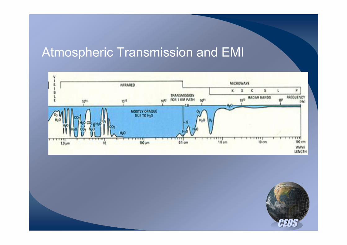
Atmospheric Transmission and EMI

CEOSCEOS

Review of Sea Ice Microwave

Scattering Theory

• Microwave scattering from Sea Ice is

controlled by three factors:

– 1) The Complex Dielectric Constant

– 2) The inhomogeneities of Scattering

Inclusions

– 3) The Frequency, Polarization and Sensor

Geometry of the SAR

CEOSCEOS

Complex Dielectric

!*=!"+j!#

Ice Type

Ice Thickness

Ice Salinity

Ice Temperature

Snow Depth

.

.

Multi-

frequency

& polarized

EM

Signatures

Forward Approach

Inverse Approach

Freeze onset date Radiative

transfer model

The electromagnetic properties of sea ice

IEEE TGARS, ONR ARI special issue. 36(5): 1750-1763

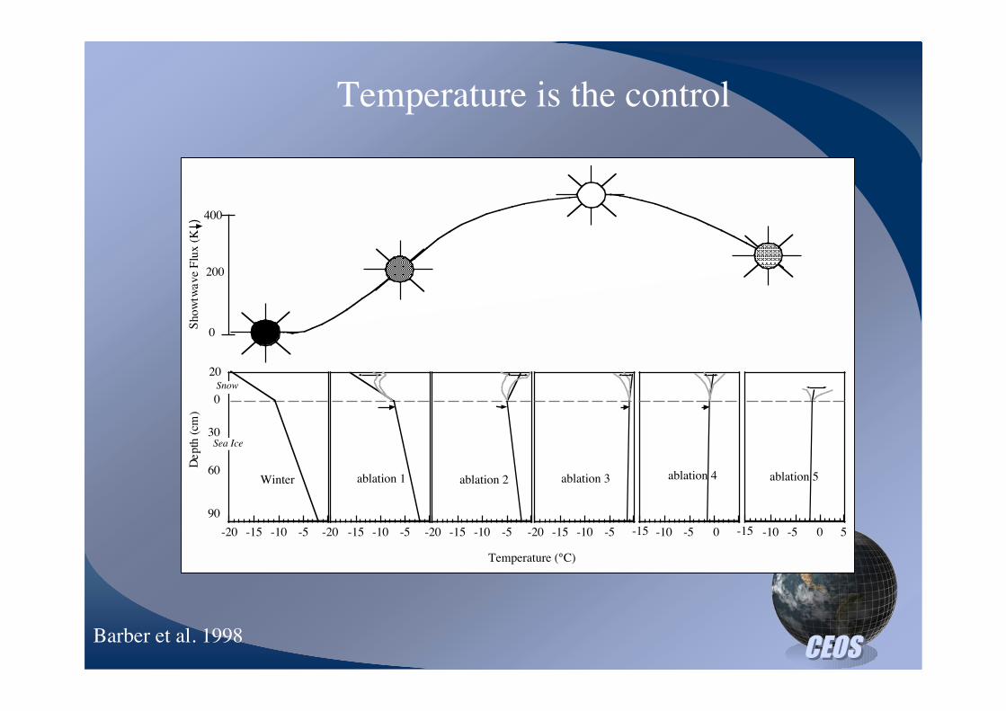
CEOSCEOSBarber et al. 1998

0-5-10

20

0

30

60

90

Depth

(cm

)

-5-10-15-20 -5-10-15 -5-10-15-20-20

Temperature (°C)

-15-5-10-15-20

Average T°

Diurnal !

Show

twave

Flu

x (

K ) 400

200

0

Snow

Sea Ice

5

Winter ablation 1 ablation 2 ablation 3 ablation 4 ablation 5

0-5-10 -15

Temperature is the control

CEOSCEOS

CEOSCEOS

An electro-thermophysical model of snow

covered sea ice

snow

ice

QH QELd LuKd Ku

K*o

K*B=Q*is

K*1x=Q*1x

Qso

Qs1x

QsB

Qio

Z=1x

Z=2x

Z=Nx

Z=0x

Z=B

QM

Q* Q*

Density (kg m-3)

Salinity (ppt)

Liquid (% by vol.)

Mass

CEOSCEOS

Snow

Sea Ice

CEOSCEOS

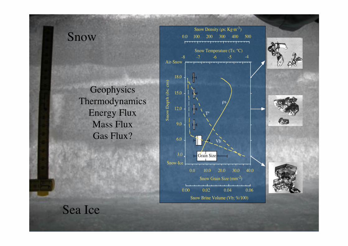
Snow

Sea Ice

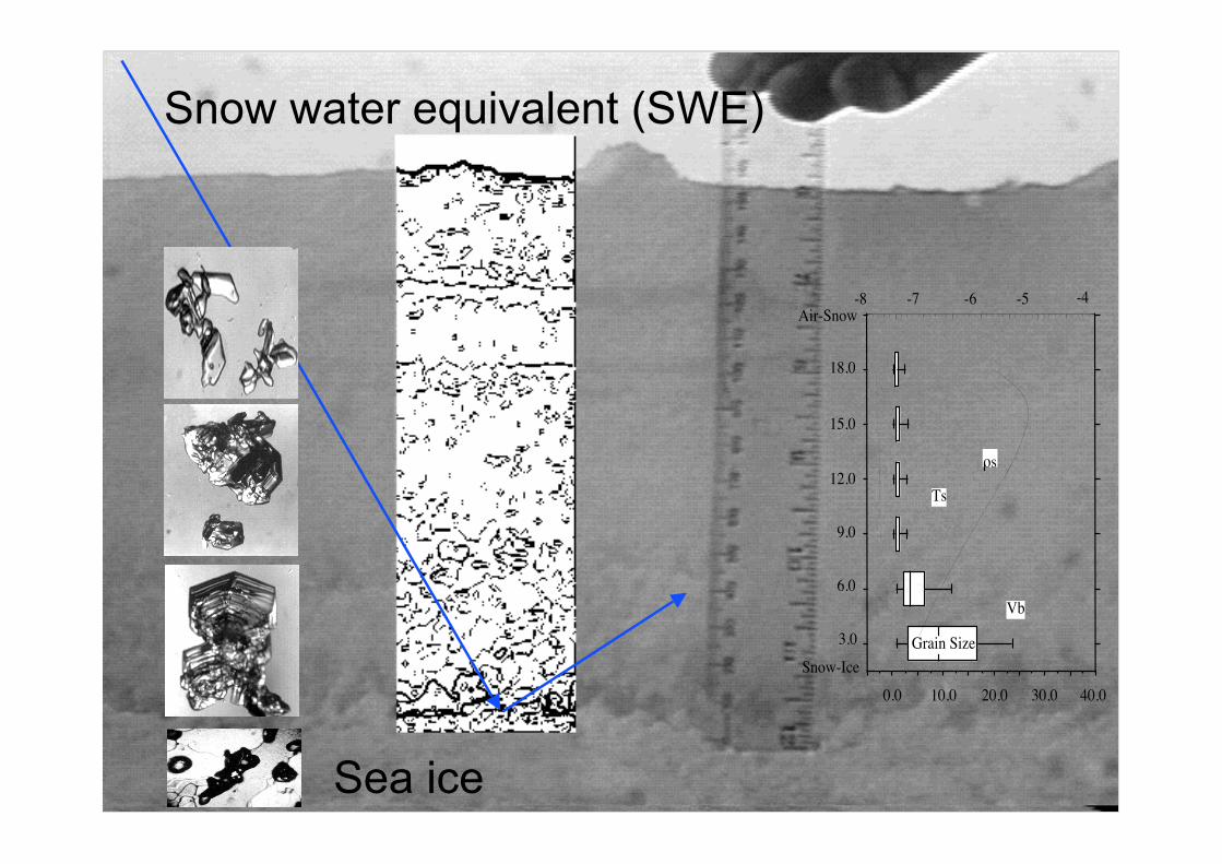
0.0

6.0

9.0

12.0

15.0

18.0

Snow

Depth

(!s;

cm

)10.0 20.0 30.0 40.0

Snow Grain Size (mm-2)

-8 -7 -6 -5 -4

Snow Temperature (Ts; °C)

0.00 0.02 0.04 0.06

Snow Brine Volume (Vb; %/100)

0.0 100 200 300 400 500

Snow Density ("s; Kg·m-3)

Grain Size3.0

Snow-Ice

Air-Snow

"s

#°

Vb

Geophysics

Thermodynamics

Energy Flux

Mass Flux

Gas Flux?

CEOSCEOS

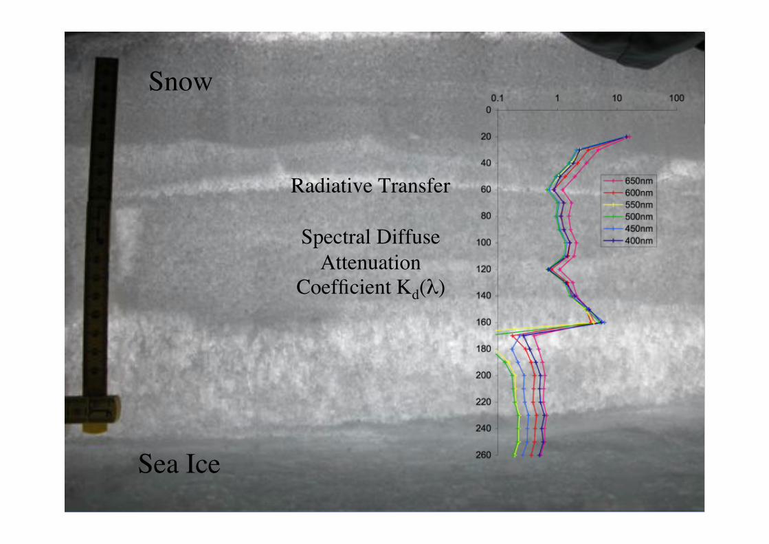
Snow

Sea Ice

Radiative Transfer

Spectral Diffuse

Attenuation

Coefficient Kd($)

CEOSCEOS

The Temporal Evolution of !º

..

-20

-15

-10

-5

Multiyear

First-Year

Winter EarlyMelt

MeltOnset

AdvancedMelt

Pen

dula

r

Funic

ula

r

Pondin

g

Dra

inag

e

!°

(ER

S-1

)

Freeze-up

CEOSCEOS

The Temporal Evolution of Tb

CEOSCEOS

Coupled sea Ice thermophysical and

dielectrics model.

•The complex dielectric constant

is defined as:

!% = !" + j!#

!" is the permittivity

!# is the loss

CEOSCEOS

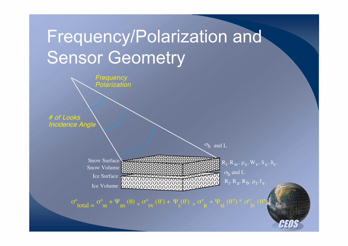
Frequency/Polarization and

Sensor Geometry

!°total =

!°ss

+ "as

(#) *

!°sv

(#') + "s(#')

* !°

is + "

si (#") * !°

iv (#")

Snow Surface

Snow Volume

Ice Surface

Ice Volume

!h and L

Ri, Rw, $s, Wv, Ss, %s,

!h and L

Ri, Ra, Rb, $i, Is,

FrequencyPolarization

# of LooksIncidence Angle

CEOSCEOS

The dielectric constant

CEOSCEOS

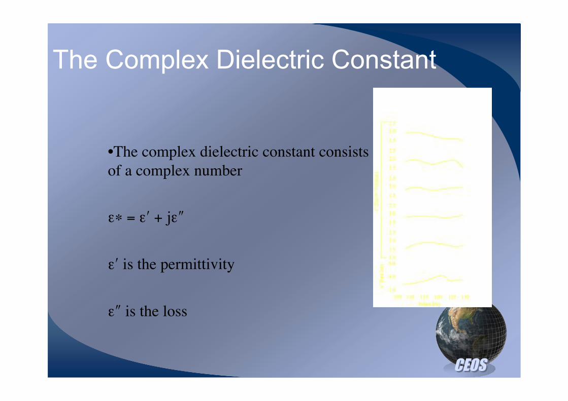
The Complex Dielectric Constant

•The complex dielectric constant consists

of a complex number

!% = !" + j!#

!" is the permittivity

!# is the loss

CEOSCEOS


!

" # w = #w$ +#w0 %#w$

1+ (2&f'w )2

!

" " # w =2$f%w(#w0 &#w')

1+ (2$f%w )2

!

"w0(T ) = 88.045# 0.4147T + 6.295$10

#4T2+1.075$10

#5T3

!

2"#w(T ) = 1.1109$10

%10% 3.824 $10

%12T + 6.938$10

%14T2% 5.096$10

%6T3

where w0 is static dielectric constant of pure water, w! is high-frequency (or optical) limit of w ( w! = 4.9) ,

w is relaxation time of pure water (s); f is electromagnetic frequency (Hz).

The Debye Model - Water

CEOSCEOS


!

" # b = #w$ +#b0 %#w$

1+ (2&f'b )2

!

" " # b =2$f%b(#b0 &#w')

1+ (2$f%b )2

+(b

2$#0f

!

"b0 =

(939.66#19.068T )

(10.737# T )

!

"# =(82.79+ 8.19T

2)

(15.68+T2)

!

2"# = 0.10990+ 0.13603$10%2T + 0.20894 $10

%3T2+ 0.28167$10

%5T3

The Debye Model - Brine

CEOSCEOS

Dielectric Mixture Models

Inclusion dielectric

in an air

background

!

"si = " i +3"si fa(1#" i )

2" si +1+" si fb("b #" i )

3

1

" si(1# Ni )+ Ni"b+

1

"si(1+ N1)+"b(1# N

1)

$

% &

'

( )

!

"ds

= 1+ 3"dsvi

"i#1

"i+ 2"

ds

$

% &

'

( )

!

"ws

= "ds

+mv"ws

3("

w#"

ds) ["

ws+ ("

w#"

ws)N

i]#1

i=1

3

$

Dry snow

Wet snow

Sea Ice

CEOSCEOS


. .

2

2.5

3

3.5

4

4.5

5

0 10 20 30 40 50

Ta = -5.0°C

Snow depth (Ds) in cm.

Si= 10pptDi = 100cmFi = 5GHz!s = 350kg

Ta = -10.0°C

Ta = -20.0°C

Ice

Surf

ace

Per

mit

tivit

y ("')

Change in !' and !'’ at the sea ice surface as a function of air temperature and snow thickness.

CEOSCEOS


. .

0

0.5

1.0

1.5

2.0

2.5

3.0

3.5

0 5 10 15 20

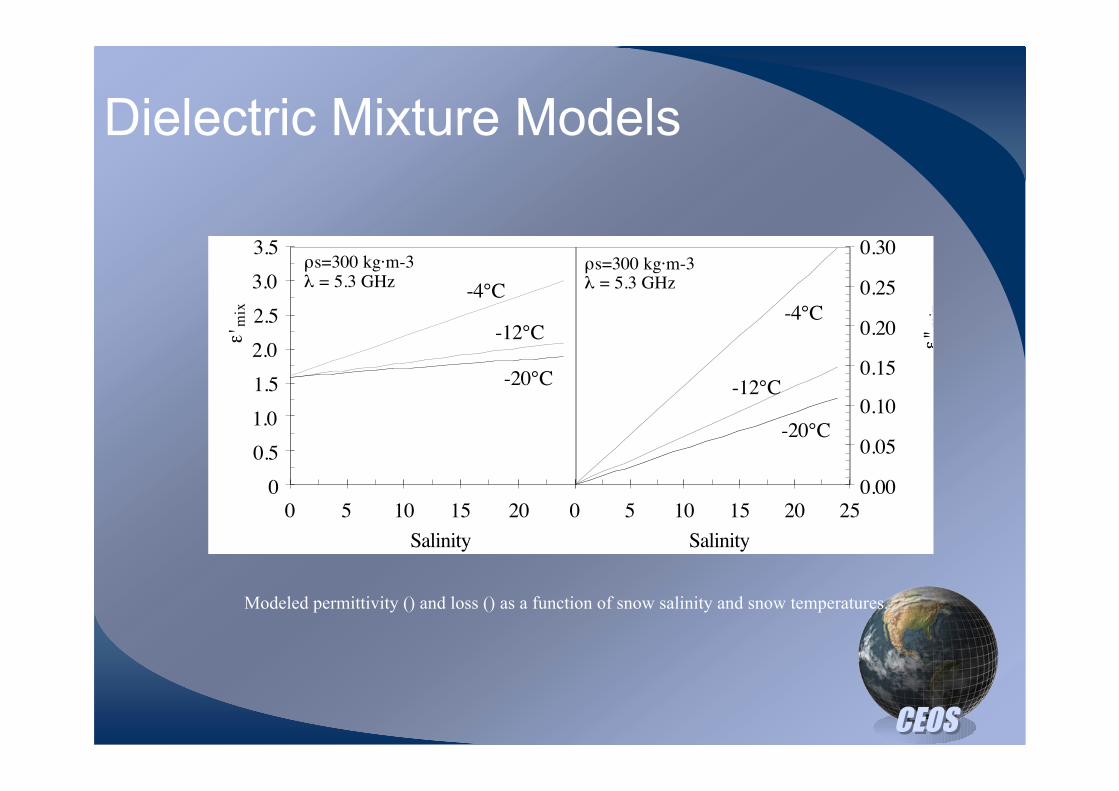
!s=300 kg·m-3" = 5.3 GHz

Salinity

#' m

ix

0 5 10 15 20 25

Salinity

#"

mix

!s=300 kg·m-3" = 5.3 GHz-4°C

-12°C

-20°C

0.00

0.05

0.10

0.15

0.20

0.25

0.30

-4°C

-12°C

-20°C

Modeled permittivity () and loss () as a function of snow salinity and snow temperatures.

CEOSCEOS


Water Volume (%/100)

!"

1

1.5

2

2.5

3

3.5

0.0

01

0.0

11

0.0

21

0.0

31

0.0

41

0.0

51

0.0

61

0.0

71

0.0

81

0.0

91

0.1

01

0.1 gm·cm-3

0.2 gm·cm-3

0.3 gm·cm-3

0.4 gm·cm-3

0.5 gm·cm-3

Frequency = 5.3 GHz

Bulk dielectric permittivity (!') of snow as a function of water volume and snow density

CEOSCEOS

Link between dielectrics and

scattering/emission

Snow

Columnar layer

S1 , TPhy1

S2 , TPhy2

S3, TPhy3

!1", !1""

!2", !2""

!3", !3""

Frazil layer

T(z)

Layer properties defined by the Fresnel reflection (&) coefficient

'｡total = '｡ss

+ (as

()) * '｡sv

()') + (s()')

* '｡is + (

si ()") * '｡iv ()")

CEOSCEOS

Scattering & Emission

Models

CEOSCEOS

Classes of Models

DMRT; Dense Medium Radiative Transfer; DMT: Dense Medium Theory, PS: physical optics under the scalar

approximation, GO: geometric optics approximation, SP: small perturbation method

Volume scatteringRough surface

scatteringMulti-layer reflection

Integrated surface-

volume signature

model

Reflection-volume

signature

Multilayer Fresnel formula

•No scattering effects

•Applicable only to

Young saline ice

Many layer SFT

•Scattering effects

to some extent

•Applicable to

Young saline ice,

frozen melt ponds

(up to 40 GHz)

•bubbly ice (up to

20 GHz)

Rayleigh scattering

DMRT

DMT

•No reflection effects

•Poor agreements (at

H-pol) over young ice,

frozen melt ponds

•Bubbly ice up to 19

GHz

DMT-integration model

PS

GO

SP

Integration

•No significant

improvement from

DMT

•This indicated no

significant rough

surface scattering

effects

Numerical method

Empirical method

•Good potential

•Backscattering

problem

•Snow application

(Winebrenner et al., 1992; Nassar et al., 2000; Wiesmann and Matzler, 1999)

CEOSCEOS

Emission/Scattering Theory

Snow

Columnar layer

S1 , TPhy1

S2 , TPhy2

S3, TPhy3

!1", !1""

!2", !2""

!3", !3""

Frazil layer

T(z)

oooo

sosvossokTkTk !!!! )()()( 22

++=

Backscattering

siaaTkkT )()0,( 00 !=

! +""= #$$%%&

' ddkkkkRkvaaha

sin)],(),([4

11)( 00

2

0

Emission

snow surface

snow volume

Snow/sea ice

interface

Interface

reflection

Volume

Scattering loss

! += "##$$%

ddkkkkRoavoahs

sin)],(),([4

1

CEOSCEOS

'｡total = '｡ss

+ (as

()) * '｡sv

()') + (s()')

* '｡is + (

si ()") * '｡iv ()")

Snow Surface

Snow Volume

Ice Surface

Ice Volume

'h and L

Ri, Rw, *s, Wv, Ss, +s,

'h and L

Ri, Ra, Rb, *i, Is,

FrequencyPolarization

# of LooksIncidence Angle

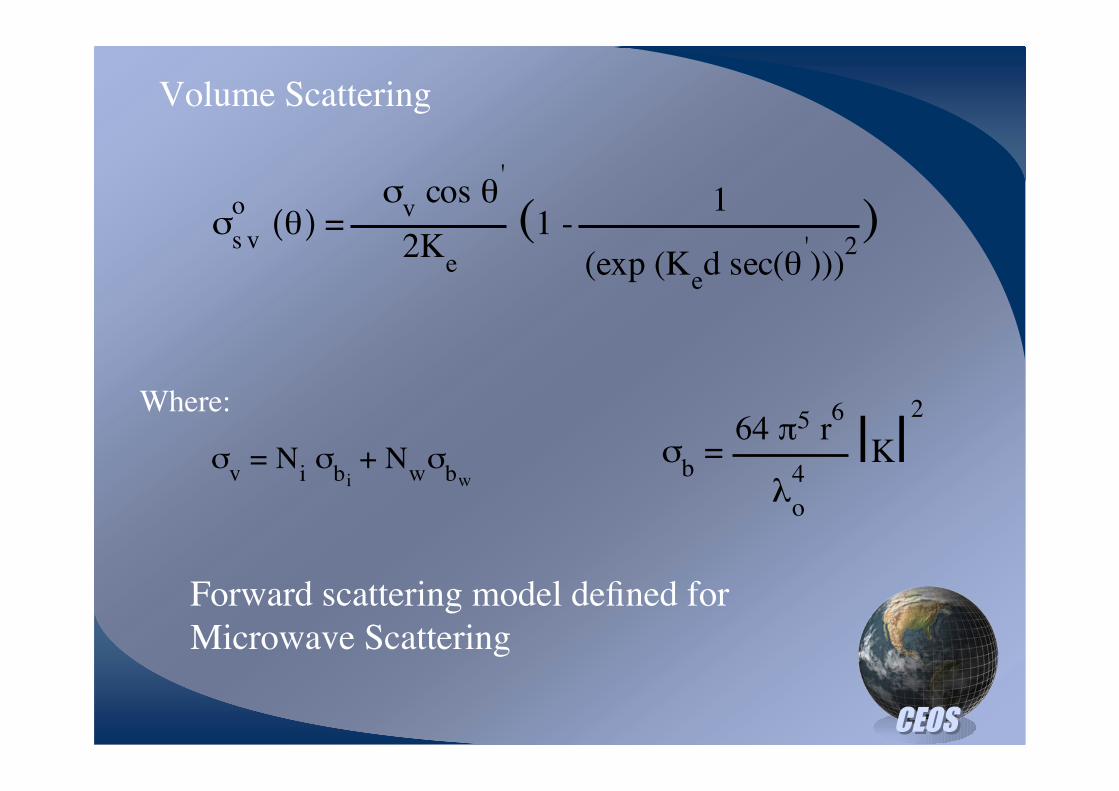
Forward scattering model defined for

Microwave Scattering

CEOSCEOS

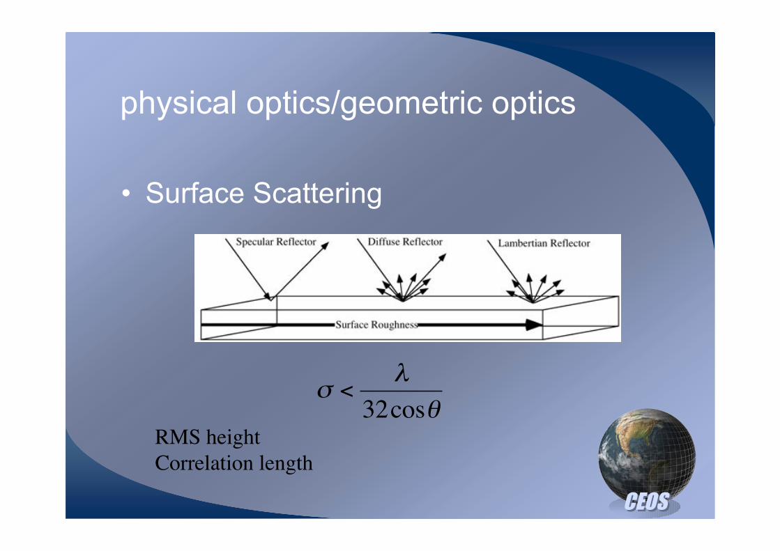
physical optics/geometric optics

• Surface Scattering

!

" <#

32cos$RMS height

Correlation length

CEOSCEOS

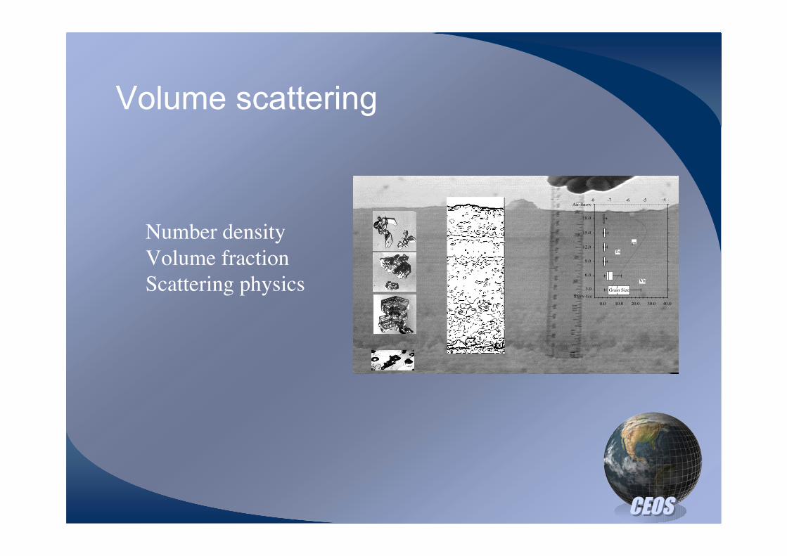
Volume scattering

0.0

6.0

9.0

12.0

15.0

18.0

10.0 20.0 30.0 40.0

-8 -7 -6 -5 -4

Ts

Vb

!s

Grain Size3.0

Snow-Ice

Air-Snow

Number density

Volume fraction

Scattering physics

CEOSCEOS



!" (#) = 2 | $%%

|2 cos2 # exp (-4 K

o

2 !

2 cos

2 #)

• &n=1

!

n!

(4Ko

2 !

2cos

2 #)

n

•

(4Ko

2 sin

2 # + n

2/ l

2)3/2

(Ko

2 n / l)

s

!HH

= "

2 x cos # + "

1 x cos # '

"2 x cos # - "

1 x cos # '

Where:

!1 =

"' + ""2

1, for material #1 (air)

Surface Scattering

CEOSCEOS



!v

o(") =

2Ke

!v cos "

'

(1 -

(exp (Ked sec("

')))

2

1 )s

!v = N

i !

bi

+ Nw !

bw

Where:

!b =

"o

4

64 #5 r6

|K|2

Volume Scattering

CEOSCEOS

Features in the mm range affect scattering

0.0

6.0

9.0

12.0

15.0

18.0

Snow

Dep

th (!s;

cm

)

10.0 20.0 30.0 40.0

Snow Grain Size (mm-2)

-8 -7 -6 -5 -4

Snow Temperature (Ts; °C)

0.00 0.02 0.04 0.06

Snow Brine Volume (Vb; %/100)

0.0 100 200 300 400 500

Snow Density ("s; Kg·m-3)

Grain Size3.0

Snow-Ice

Air-Snow

"s

#°

Vb

Ehn et al.

0.0

6.0

9.0

12.0

15.0

18.0

10.0 20.0 30.0 40.0

-8 -7 -6 -5 -4

Ts

Vb

!s

Grain Size3.0

Snow-Ice

Air-Snow

CEOSCEOS

Many layer SFT model (scattering and emission)

(Winebrenner et al., 1992)

Description

-assumes the snow/sea ice is a piecewise-continuous random

medium and accounts for the interference between waves reflected

and transmitted coherently by the various planar layers

- accounts for the mean propagation and first-order multiple scattering

effects by using bilocal and distorted born approximations

CEOSCEOS

(Winebrenner et al., 1992)

CEOS

Input parameters

General: frequency (GHz), angles

For ice: temperature, salinity, density, ice grain size (mm), air

bubble size, brine aspect ratio and tilted angle.

For snow: temperature, density, snow wetness (fractional volume)*,

snow grain size (mm).

*liquid water distributed between grains as well as around grains

(Stogryn, 1985).

Output parameters

Microwave brightness temperature (emissivity) and backscattering

(sigma) for V and H polarizations.

Many layer SFT model (scattering and emission)

CEOSCEOS

Extending signatures temporally - Ice emissivity simulated by the

many layer strong fluctuation theory model. The brine skim/wet slush

was set to be 5 mm, and ice salinity based on field data

Hwang and Barber, JGR, in press

CEOSCEOS

Some examples

CEOSCEOS

Snow Thickness

• Scattering Response. .

-26 -24 -22 -20 -18 -16 -14 -12 -10 -8 -6 -4

-24

-22

-20

-18

-16

-14

-12

-10

-8

-6

-4

-26

!° (dB) - May 6 (Clear)

!°

(dB

) -

M

ay 9

(C

loudy)

N= 900 x 2

May 6 (Clear) May 9 (Cloudy)

Barber and Thomas, 1998

0.0

6.0

9.0

12.0

15.0

18.0

10.0 20.0 30.0 40.0

-8 -7 -6 -5 -4

Ts

Vb

!s

Grain Size3.0

Snow-Ice

Air-Snow

Snow water equivalent (SWE)

Sea ice

CEOSCEOS

SWE and Scattering

• Observed Response to Snow Thickness

Barber et al. 1998

CEOSCEOSYackel and Barber, 2000

CEOSCEOS

5 10 15 20

Site Number

0

20

40

60

Dep

th (

cm

)

0

60

115

170

225S

WE

(mm

)

Snow

thicknessSWE

SWE and Radiometry (20 sites)

Barber et al. 2000.

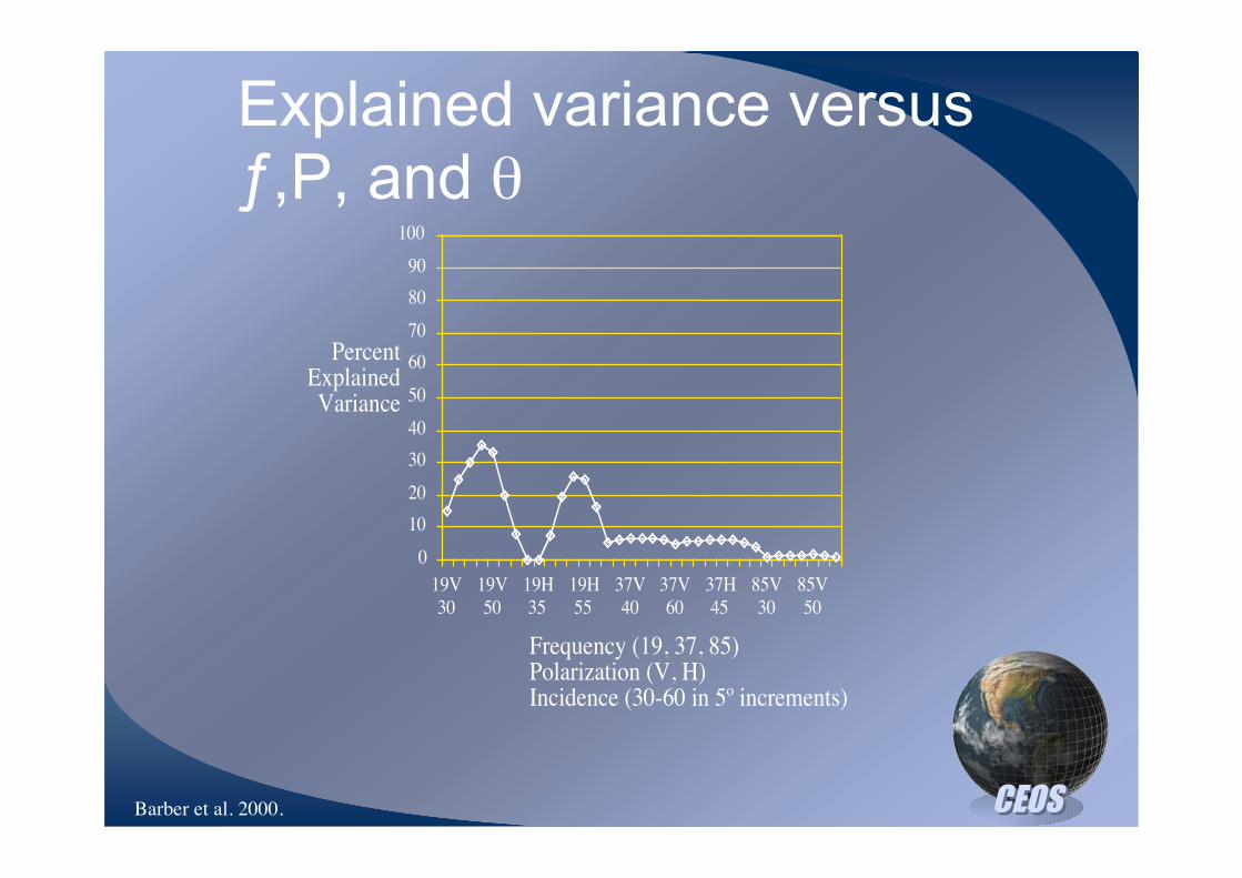
CEOSCEOS

Explained variance versusƒ,P, and )

0

10

20

30

40

50

60

70

80

90

100

19V

30

19V

50

19H

35

19H

55

37V

40

37V

60

37H

45

85V

30

85V

50

Frequency (19, 37, 85)Polarization (V, H)Incidence (30-60 in 5º increments)

PercentExplainedVariance

Barber et al. 2000.

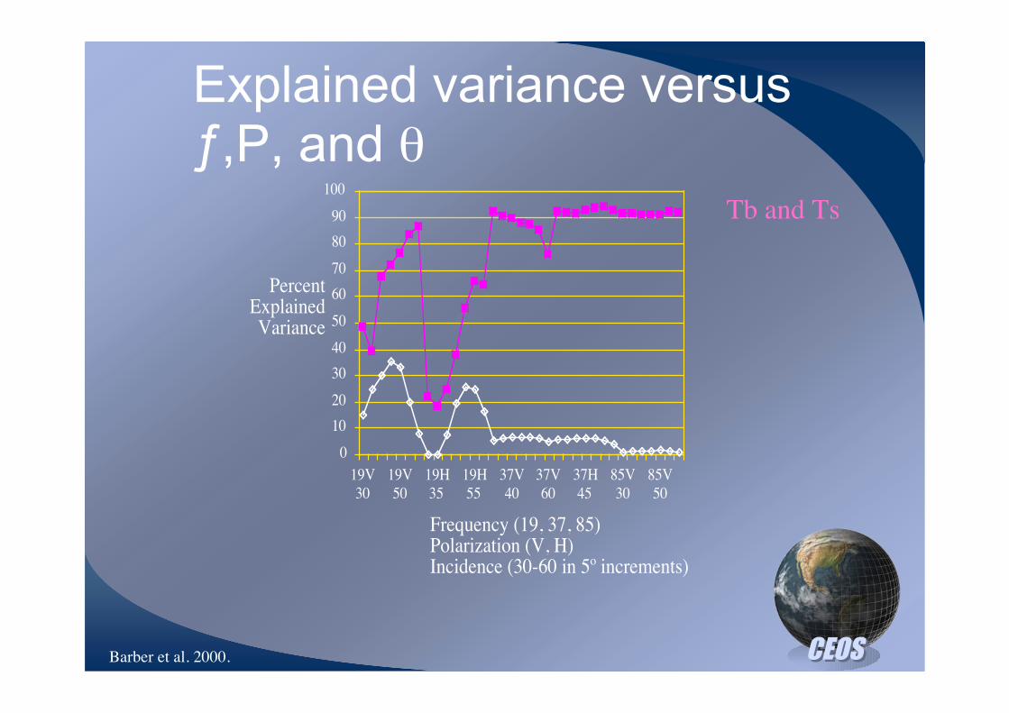
CEOSCEOS

Explained variance versusƒ,P, and )

0

10

20

30

40

50

60

70

80

90

100

19V

30

19V

50

19H

35

19H

55

37V

40

37V

60

37H

45

85V

30

85V

50

Frequency (19, 37, 85)Polarization (V, H)Incidence (30-60 in 5º increments)

PercentExplainedVariance

Barber et al. 2000.

Tb and Ts

CEOSCEOS

Late season sea ice

Melt Pond DielectricsMelt Pond Dielectrics Snow Patch DielectricsSnow Patch Dielectrics

!% = !" + j!#

!% = 65.8065.80+ j36.5136.51

for pure water at

0°C, 5.3 GHz

for wet snow at

-1°C, 0.3 gm.m-3, 0.1 Wv

!% = 1.911.91+ j0.110.11

CEOSCEOS

Melt Ponds on Landfast First Year Sea Ice.

CEOSCEOS

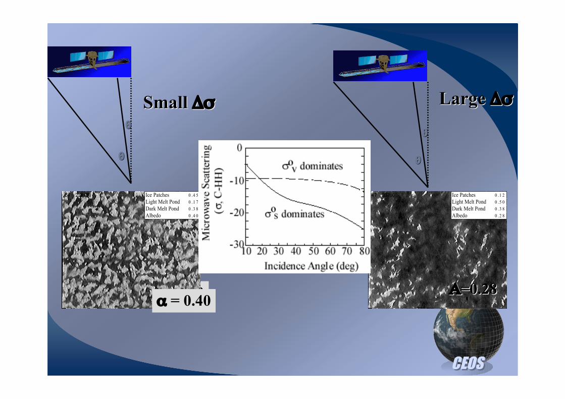
, = 0.40

))

))

Small Small -'-'

Ice Patches 0 .4 5

Light Melt Pond 0 .1 7

Dark Melt Pond 0 .3 8

Albedo 0 .4 0

, = 0.40

Ice Patches 0 .1 2

Light Melt Pond 0 .5 0

Dark Melt Pond 0 .3 8

Albedo 0 .2 8

..=0.28=0.28

))

))

LargeLarge -'-'

CEOSCEOS

The Temporal Evolution of

Sigma Naught

• Several variables must be taken into

consideration:

– The effect of incidence angle

– The effect of wind

– The contribution to backscatter (!º) by

volume and surface scattering as dictated

by the dielectrics of the system

CEOSCEOS

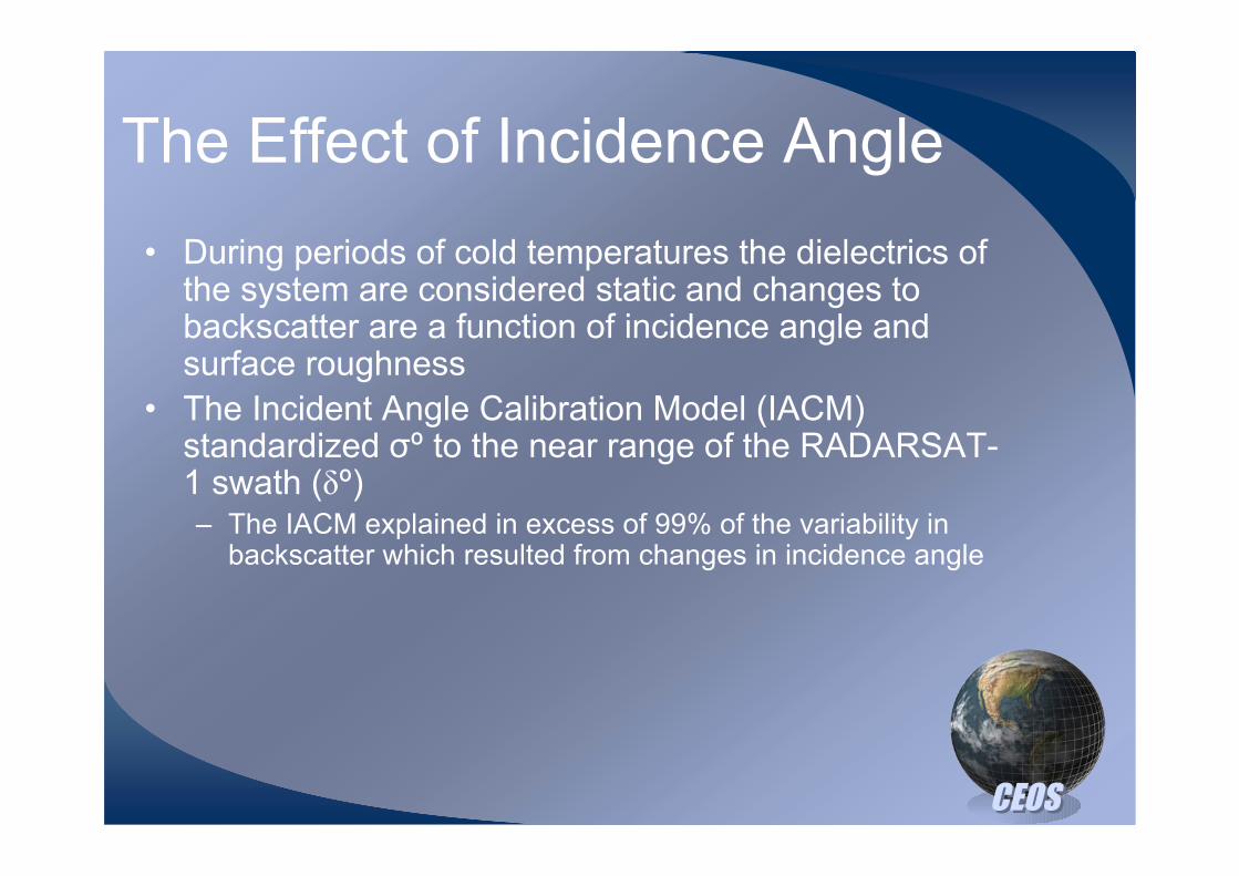
The Effect of Incidence Angle

• During periods of cold temperatures the dielectrics ofthe system are considered static and changes tobackscatter are a function of incidence angle andsurface roughness

• The Incident Angle Calibration Model (IACM)standardized !º to the near range of the RADARSAT-1 swath (!º)– The IACM explained in excess of 99% of the variability in

backscatter which resulted from changes in incidence angle

CEOSCEOS

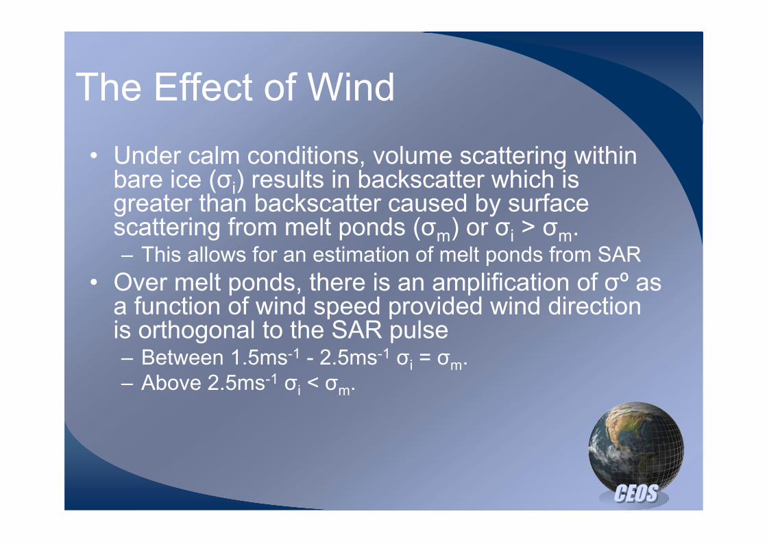
The Effect of Wind

• Under calm conditions, volume scattering withinbare ice (!i) results in backscatter which isgreater than backscatter caused by surfacescattering from melt ponds (!m) or !i > !m.– This allows for an estimation of melt ponds from SAR

• Over melt ponds, there is an amplification of !º asa function of wind speed provided wind directionis orthogonal to the SAR pulse– Between 1.5ms-1 - 2.5ms-1 !i = !m.

– Above 2.5ms-1 !i < !m.

CEOSCEOS

Pond fraction (PF),

wind speed (W),

wind direction in

degrees (D) and

weather are all

indicated for each

image. The images

have been calibrated

to ASF gamma

values and areas of

low backscatter

appear dark. All

images are courtesy

of the Canadian

Space Agency (©

CSA, 2002)

CEOSCEOS

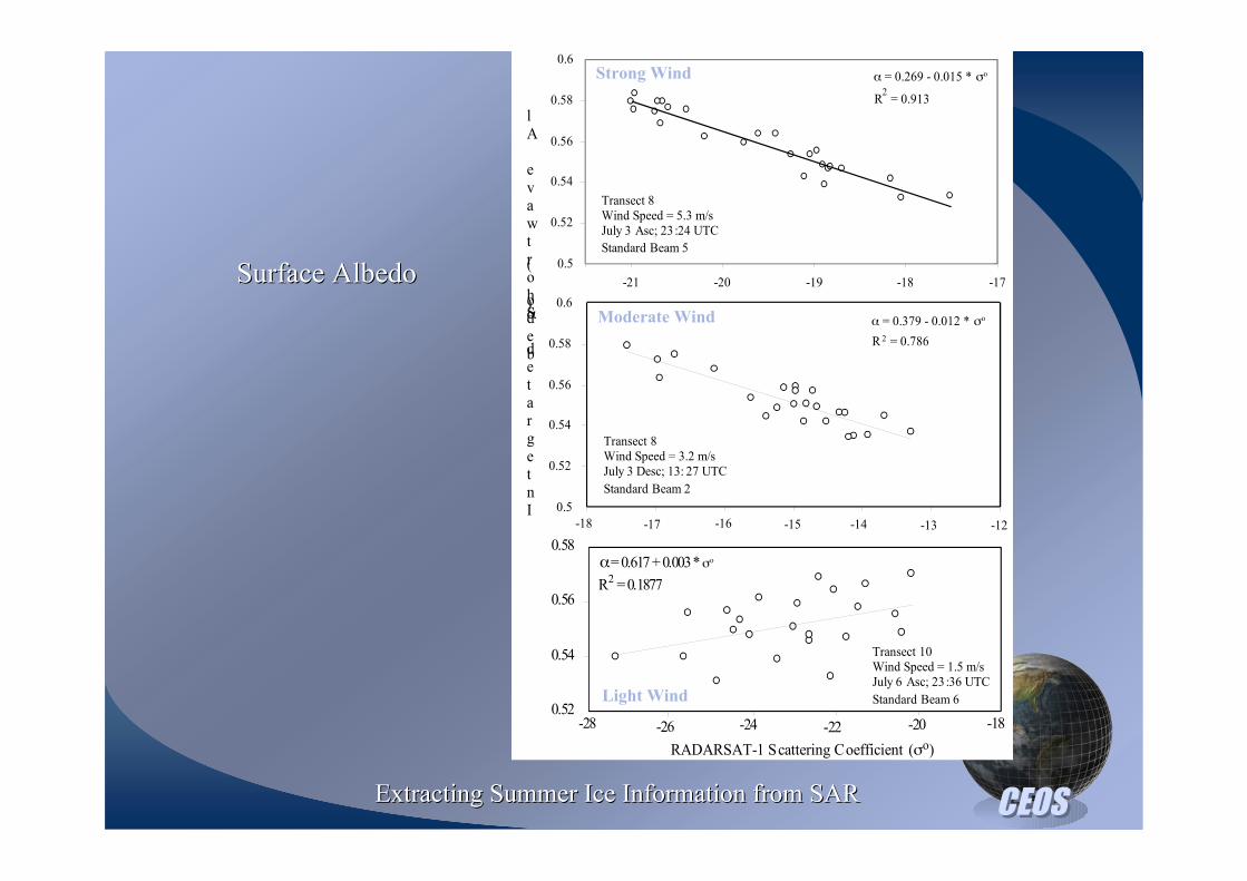
Surface AlbedoSurface Albedo

R2 = 0.913

! = 0.269 - 0.015 * "o

0.5

0.52

0.54

0.56

0.58

0.6

-21 -20 -19 -18 -17

Integrated Shortwave Al

bedo (

!)

0.5

0.52

0.54

0.56

0.58

0.6

! = 0.379 - 0.012 * "o

R 2 = 0.786

-18 -17 -16 -15 -14 -13 -12

Transect 8

Wind Speed = 3.2 m/s

July 3 Desc; 13: 27 UTC

Standard Beam 2

-28 -26 -24 -22 -20 -180.52

0.54

0.56

0.58! = 0.617 + 0.003 * "o

R2 = 0.1877

Transect 10


July 6 Asc; 23 :36 UTC

Standard Beam 6

RADARSAT-1 Scattering Coefficient ("o)

Transect 8


July 3 Asc; 23 :24 UTC

Standard Beam 5

Light Wind

Moderate Wind

Strong Wind

Extracting Summer Ice Information from SARExtracting Summer Ice Information from SAR

CEOSCEOS

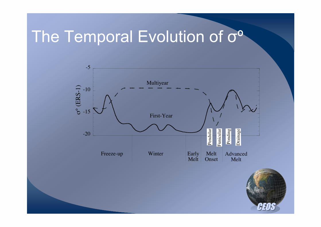
The Temporal Evolution of !º

..

-20

-15

-10

-5

Multiyear

First-Year

Winter EarlyMelt

MeltOnset

AdvancedMelt

Pen

dula

r

Funic

ula

r

Pondin

g

Dra

inag

e

!°

(ER

S-1

)

Freeze-up

CEOSCEOS

The Temporal Evolution of Tb

CEOSCEOS

Conclusions

• Electro-thermophysical model (heuristic to physical)

• Emission/scattering models

• Geophysical vs Thermodynamic state (processes)

• Initialization and steering of models, data

assimilation

• Scale related science (micro to hemispheric)

• Merger of environmental science and technologies

CEOSCEOS

A metaphor for science and technology

CEOSCEOS

Acknowledgements:

John Yackel

John Hanesiak

Tim Papkyriakou

Ryan Galley

Alex Langlois

Phil Hwang

John Iacozza

CJ Mundy

Rob Kirk

Sheldon Drobot

Theresa Fisico

Theresa Nichols

Chistina Blouw

Isabelle Harouche

Andrew Thomas

Klaus Hochheim

Jens Ehn

Mats Granskog

Wanli Woo

Randy Scharien

Katherine Wilson

Wayne Chan

Jennifer Lukovich

The real forces

behind this work

CEOSCEOS

For more information

[email protected]

www.umanitoba.ca/ceos

CEOSCEOS

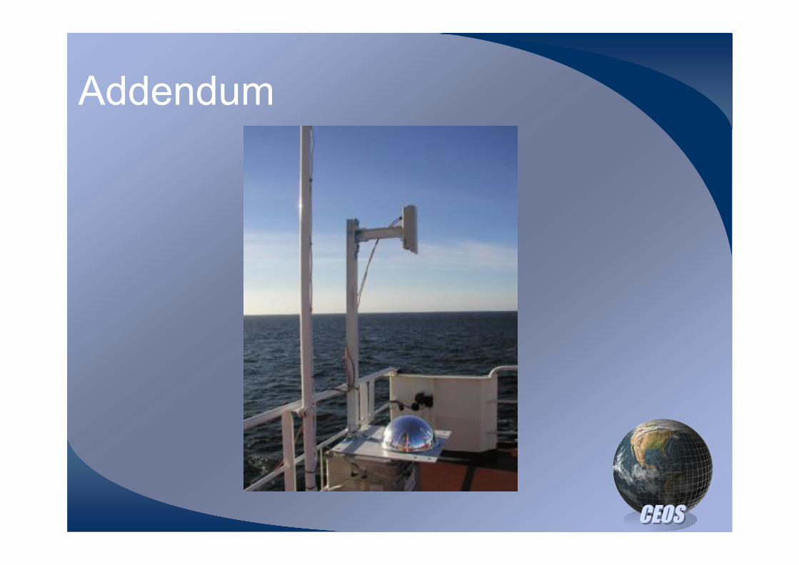
Addendum

Sea Ice, Climate Change and Remote Sensing - Earth Online · Sea Ice, Climate Change and Remote Sensing ... Arctic Climate Change and Remote Sensing 2) ... medium and accounts for

Documents