Sd4 tignes 2013-2

Epstein Department of ISE

Stochastic Decomposition

Suvrajeet Sen

Lecture at the Winter School

April 2013


The Plan – Part I ( 70 minutes)• Review of Basics: 2-stage Stochastic Linear Programs (SLP)• Deterministic Algorithms for 2-stage SLP

– Subgradients of the Expected Recourse Function– Subgradient Methods– Deterministic Decomposition (Kelley/Benders/L-shaped)

• Stochastic Algorithms for 2-stage SLP– Stochastic Quasi-gradient Methods– Sample Average Approximation– Stochastic Decomposition (SD) Algorithm

• Computational Results


Review of Basics: 2-stage Stochastic Linear Programs


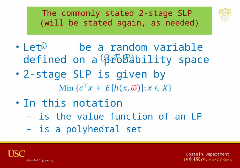
• Let be a random variable defined on a probability space

• 2-stage SLP is given by

• In this notation– is the value function of an LP– is a polyhedral set

The commonly stated 2-stage SLP (will be stated again, as needed)


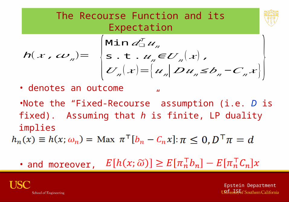
The Recourse Function and its Expectation

• denotes an outcome

•Note the “Fixed-Recourse” assumption (i.e. D is fixed). Assuming that h is finite, LP duality implies

• and moreover,

h (𝑥 ,𝜔𝑛)= {Min𝑑❑⊤𝑢𝑛

s . t .𝑢𝑛∈𝑈𝑛 (𝑥 ) ,𝑈𝑛 (𝑥 )={𝑢𝑛|𝐷𝑢𝑛≤𝑏𝑛−𝐶𝑛 𝑥 }}


Wait a minute!• Can we compute • If we have a few outcomes, Yes.

– Deterministic Algorithms for SP– Or in specialized models (e.g. newsvendor problems) we can

integrate (with low-dimensional integration)• What if we have a large number of outcomes, then what

do these operations mean? Multi-dimensional Integration LP Value and Subgradients

– This operation MUST be approximated (Dyer/Stougie [06])


One Approach: Use Sampling

• Replace each by sampled estimates– Stochastic algorithms for SP

• Some cautionary advice for sampling! – Introduces sampling error in estimation – Could sampling errors introduce loss of

convexity in approximation? • Yes, if we are not careful!


Deterministic Algorithms for 2-stage SLP

Subgradient Method, Kelley/Benders/L-shaped Method


Subgradient Method (Shor/Polyak/Nesterov/Nemirovski…)

•At iteration k let be given

•Let

•Then, where denotes the projection operator on the set of the decisions and,

•As mentioned earlier, is very difficult to compute!

•No concern about loss of convexity due to sampling

Interchange of Expectation and Subdifferentiation is required here


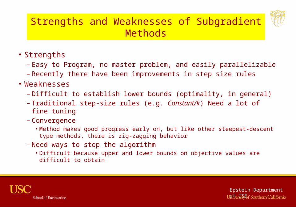
• Strengths– Easy to Program, no master problem, and easily parallelizable– Recently there have been improvements in step size rules

• Weaknesses– Difficult to establish lower bounds (optimality, in general)– Traditional step-size rules (e.g. Constant/k) Need a lot of fine tuning– Convergence

• Method makes good progress early on, but like other steepest-descent type methods, there is zig-zagging behavior

– Need ways to stop the algorithm• Difficult because upper and lower bounds on objective values are difficult to

obtain

Strengths and Weaknesses of Subgradient Methods


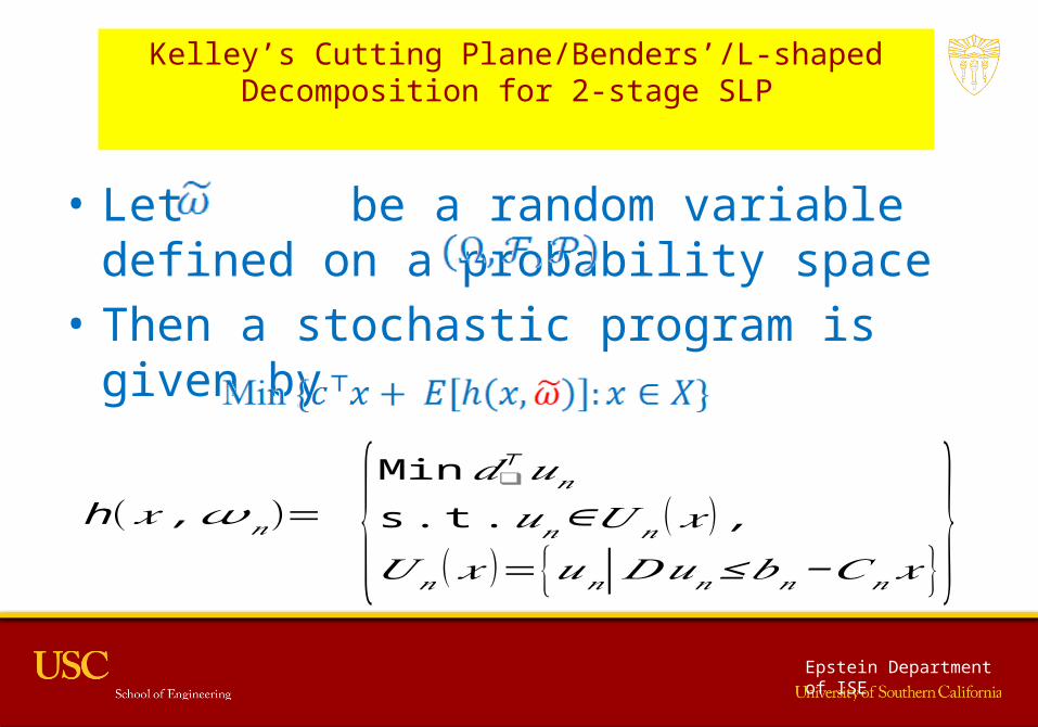
• Let be a random variable defined on a probability space

• Then a stochastic program is given by

Kelley’s Cutting Plane/Benders’/L-shaped Decomposition for 2-stage SLP




KBL Decomposition (J. Benders/Van Slyke/Wets)

•At iteration k let , and be given. Recall

•Then define

• Let

•Then,


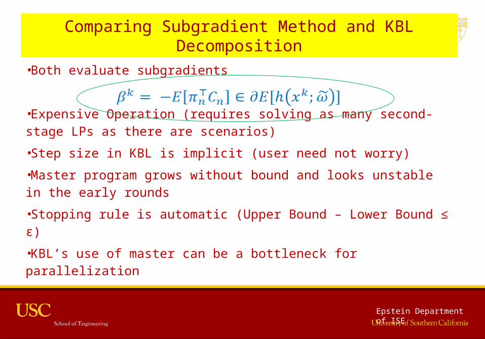
Comparing Subgradient Method and KBL Decomposition

•Both evaluate subgradients

•Expensive Operation (requires solving as many second-stage LPs as there are scenarios)

•Step size in KBL is implicit (user need not worry)

•Master program grows without bound and looks unstable in the early rounds

•Stopping rule is automatic (Upper Bound – Lower Bound ≤ ε)

•KBL’s use of master can be a bottleneck for parallelization


KBL Graphical Illustration

Expected Recourse Function

Approximation: fk-1

Approximation: fk


Regularization of the Master Problem (Ruszczynski/Kiwiel/Lemarechal …)

•Addresses the following issue:– Master program grows without bound and looks unstable in

the early rounds

•Include an incumbent and a proximity measure from the incumbent, using σ >0 as a weight:

•Particularly useful for Stochastic Decomposition.


Stochastic Algorithms for 2-stage SLP

Stochastic Quasi-Gradient, SAA, and SD


Some “concrete” instances

ProblemName

Domain # of 1st stage variab

les

# of 2nd stage

variables

# of random

variables

Universe of

scenarios

Comment

LandS Generation 4 12 3 Made-up20TERM Logistics 63 764 40 Semi-real

SSN Telecom 89 706 86 Semi-realSTORM Logistics 121 1259 117 Semi-real

Table 1: SP Test Instances

Notice the size of scenarios. Using a deterministic algorithm would be a “non-starter”


Numerous Large-scale Applications

• Wind-integration in Economic Dispatch– How should conventional resources be dispatched

in the presence of intermittent resources? • Supply chain planning

– Inventory Transhipment between Regional Distribution Centers, Local Warehouses, Outlets

• “Everyone” wants to “solve” Stochastic Unit Commitment


So what do we mean by “solve”?

I. At the very least– An algorithm which, under specified assumptions,

will provide• A first-stage decision, with known metrics of optimality.

That is, report statistically quantified error• Be reasonably fast on easily accessible machines

II. There are other things that people want


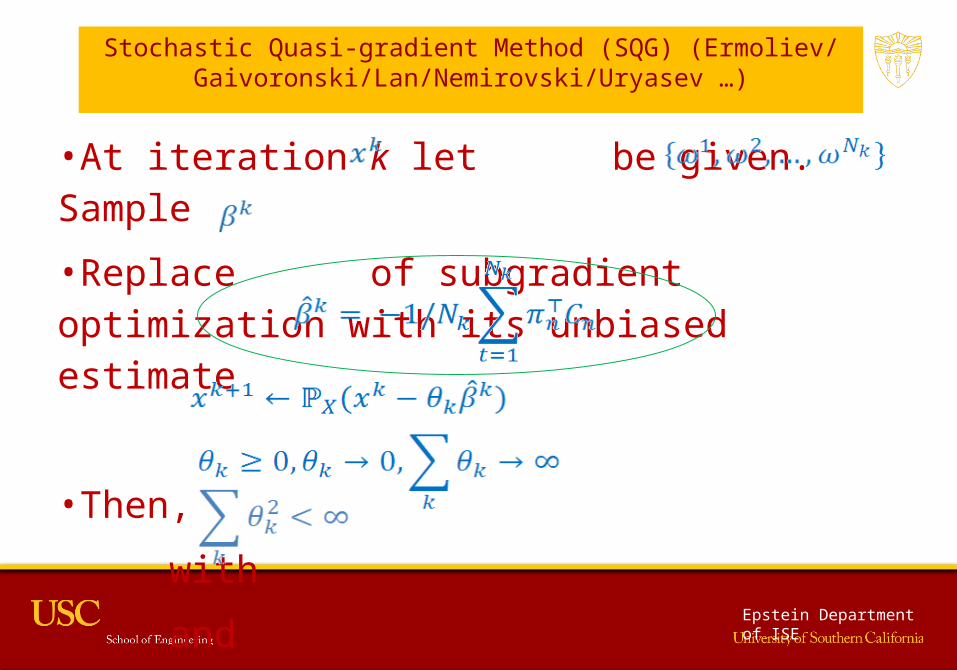
Stochastic Quasi-gradient Method (SQG) (Ermoliev/ Gaivoronski/Lan/Nemirovski/Uryasev …)

•At iteration k let be given. Sample

•Replace of subgradient optimization with its unbiased estimate

•Then,

with

and


Comments on SQG

•Because this is a sampling-based algorithm, you must replicate so that you can estimate “variability” (of what?)

•If you replicate M times, you will get M first-stage decisions. Which of these should you use?– Could evaluate each of the M first-stage decisions, and then choose the one with

smallest objective estimate

– For realistic models, this can be computationally time-consuming

•Could simply choose the mean of replications– Less expensive, but may be unreliable

•But most importantly, it does not provide lower bounds


Sample Average Approximation (SAA, Shapiro, Kleywegt, Homem-de-Mello, Linderoth, Wright ….)

•Choose a sample size N; Solve a sampled problem; Repeat M times

•Since you replicate M times, you will get M decisions. Which of these should you use?

– Could evaluate each of the M decisions, and then choose the one with smallest estimate

• For realistic models, this can be computationally time-consuming

– Could simply choose the mean of replications

• Less expensive, but may be unreliable

•Very widely cited, sometimes misused (because some non-expert users appear to choose M=1)!


Stochastic Decomposition (SD)

• Allow arbitrarily many outcomes (scenarios) including continuous random variables

• Perhaps interface with a simulator …




Some Central Questions for SP

• Instead of choosing a sample size at the start, can we decide how much to sample, on-the-fly?– The analogous question for nonlinear programming would be:

instead of choosing the number of iterations at the start, can we decide the number of iterations, on-the-fly? – Yes!

– So can we do this with sample size selection? Perhaps!• If we are to determine a sample size on-the-fly, what is the

smallest number by which to increment the sample size, and yet guarantee asymptotic convergence?


Under some assumptions …

• Fixed Recourse Matrix • Current computer Implementations assume

– Relatively complete recourse (under revision)– Second-stage cost is deterministic (under revision)


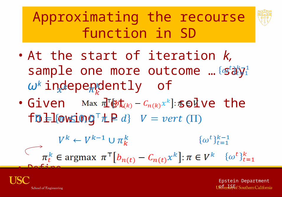
Approximating the recourse function in SD

• At the start of iteration k, sample one more outcome … say ωk independently of

• Given let solve the following LP

• Define and calculate for

• Notice the mapping of outcomes to finitely many dual vertices.


Approximation used in SD

• The estimated “cut” in SD is given by

• To calculate this “cut” requires one LP corresponding to the most recent outcome and the “argmax” operations at the bottom of the previous slide

• In addition all previous cuts need to be updated … to make old cuts consistent with the changing sample size over iterations.


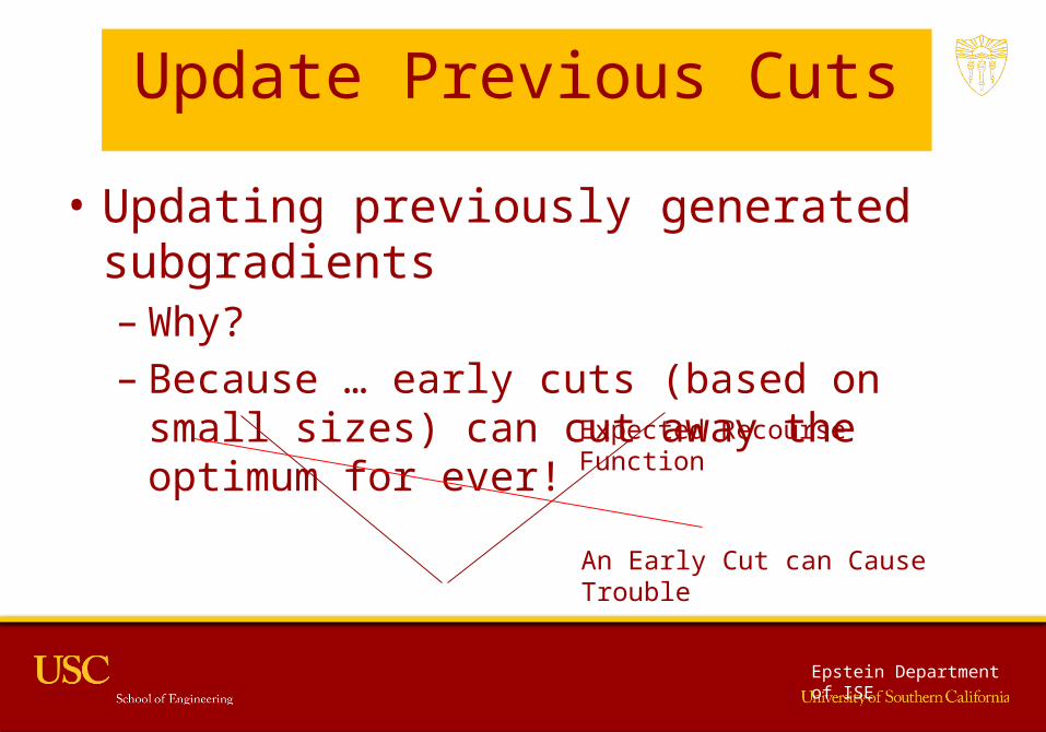
Update Previous Cuts

• Updating previously generated subgradients– Why?– Because … early cuts (based on small sizes) can cut

away the optimum for ever!

– What should we do?


An Early Cut can Cause Trouble


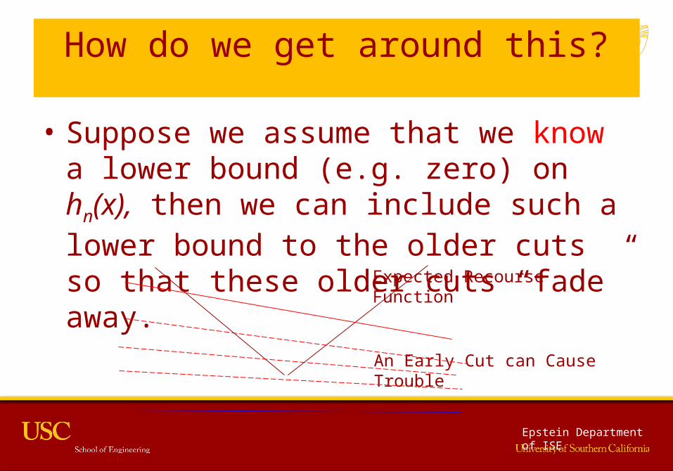
How do we get around this?

• Suppose we assume that we know a lower bound (e.g. zero) on hn(x), then we can include such a lower bound to the older cuts so that these older cuts “fade” away.


An Early Cut can Cause Trouble


Updating Previous Cuts.

• If we assume that all recourse function lower bounds are uniformly zero, – Then for t < k, the “cut” from iteration t has the following

form:


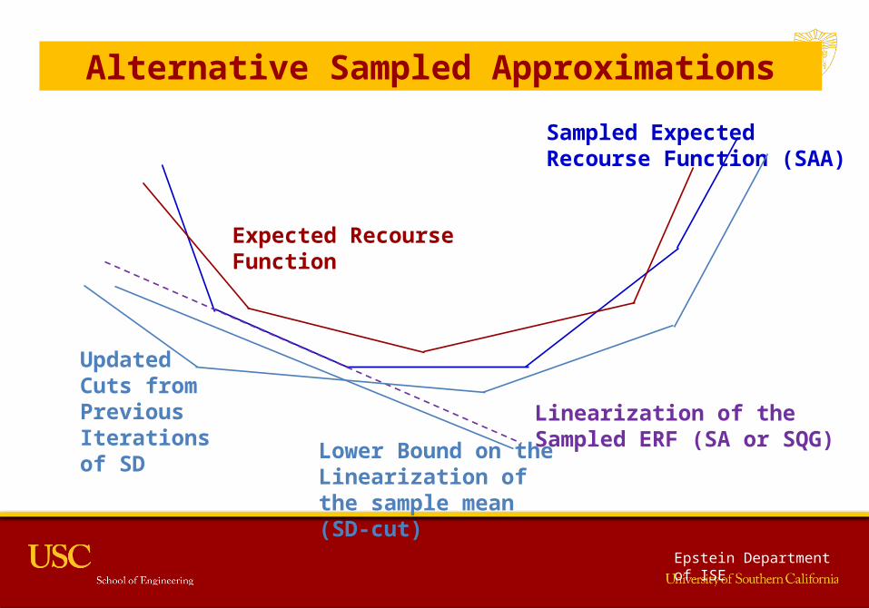
Alternative Sampled Approximations

Sampled Expected Recourse Function (SAA)

Linearization of the Sampled ERF (SA or SQG)Lower Bound on the

Linearization of the sample mean (SD-cut)

UpdatedCuts fromPrevious Iterations of SD



SUMMARY OF APPROXIMATIONS

SAA

SA

SD


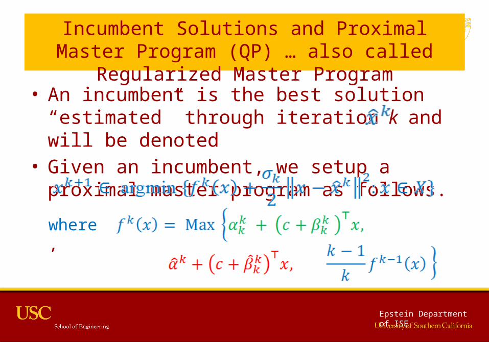
Incumbent Solutions and Proximal Master Program (QP) … also called Regularized Master Program

• An incumbent is the best solution “estimated” through iteration k and will be denoted

• Given an incumbent, we setup a proximal master program as follows.

where,


Benefits of the Proximal Master

• Can show that a finite master problem, consisting of n1+3 optimality cuts is enough! (Here n1 is the number of first-stage variables)

• Convergence can be proven to a unique limit which is optimal (with probability 1).

• Stopping rules based on QP duality are reasonably efficient.


Algorithmic Summary0. Initialize with the same candidate and incumbent x. k=1.

1. Use sampling to obtain an outcome 2. Derive an SD cut at the candidate, and the incumbent solutions.

This calls for

- solution of 2 subproblems using - Add any new dual vertex to a list

- for each prior choose the best subproblem dual vertex seen thus far

3. Update cut t by multiplying coeffs by (t/k), 4. Solve the updated QP master5. Ascertain whether new candidate becomes new incumbent6. If stopping rules are not met, increment k, and repeat from 1. (Stopping rule is based on bootstrapping primal and dual QPs)

k

k

kt

t1}{

kt ...1

Vk


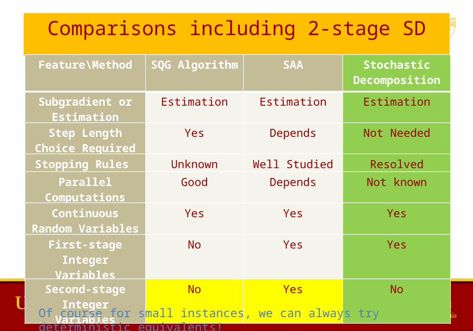
Comparisons including 2-stage SD

Feature\Method SQG Algorithm SAA Stochastic

Decomposition

Subgradient or Estimation

Estimation Estimation Estimation

Step Length Choice Required

Yes Depends Not Needed

Stopping Rules Unknown Well Studied Resolved

Parallel Computations Good Depends Not known

Continuous Random Variables

Yes Yes Yes

First-stage Integer Variables

No Yes Yes

Second-stage Integer Variables

No Yes No

Of course for small instances, we can always try deterministic equivalents!


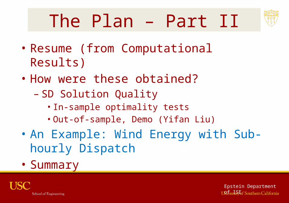
The Plan – Part II• Resume (from Computational Results)• How were these obtained?

– SD Solution Quality• In-sample optimality tests• Out-of-sample, Demo (Yifan Liu)

• An Example: Wind Energy with Sub-hourly Dispatch

• Summary


Recall this question: What do we mean by “solve”?

I. At the very least– An algorithm which, under specified assumptions,

will provide• A first-stage decision, with known metrics of optimality.

That is, report statistically quantified error• Be reasonably fast on easily accessible machines

II. There are other things that people want


What else to people want?

There are other things that people want• Evidence

– Experiment with some realistic instances• Please note that CEP1 and PGP2 are not realistic. They are for debugging!

– Some numerical controls• E.g. Can we reduce “bias”/non-optimality?

• Output for decision support– Dual estimates of first-stage– Histograms

• Recourse function • Dual prices of second-stage


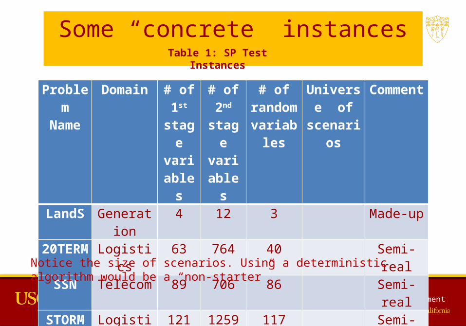
Some “concrete” instances

ProblemName

Domain # of 1st stage variab

les

# of 2nd stage

variables

# of random

variables

Universe of

scenarios

Comment

LandS Generation 4 12 3 Made-up20TERM Logistics 63 764 40 Semi-real

SSN Telecom 89 706 86 Semi-realSTORM Logistics 121 1259 117 Semi-real

Table 1: SP Test Instances

Notice the size of scenarios. Using a deterministic algorithm would be a “non-starter”


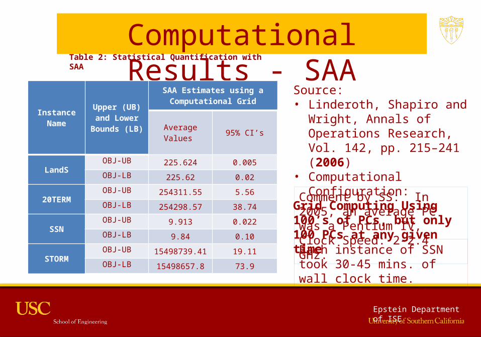
Computational Results - SAA

Instance NameUpper (UB) and Lower Bounds

(LB)

SAA Estimates using a Computational Grid

Average Values 95% CI’s

LandSOBJ-UB 225.624 0.005OBJ-LB 225.62 0.02

20TERMOBJ-UB 254311.55 5.56OBJ-LB 254298.57 38.74

SSNOBJ-UB 9.913 0.022OBJ-LB 9.84 0.10

STORMOBJ-UB 15498739.41 19.11OBJ-LB 15498657.8 73.9

Table 2: Statistical Quantification with SAA

Source: • Linderoth, Shapiro and Wright,

Annals of Operations Research, Vol. 142, pp. 215–241 (2006)

• Computational Configuration:Grid Computing Using 100’s of PCs, but only 100 PCs at any given time

Comment by SS: In 2005, an average PC was a Pentium IV, Clock Speed: 2-2.4 GHz.

Each instance of SSN took 30-45 mins. of wall clock time.Replications: 7-10


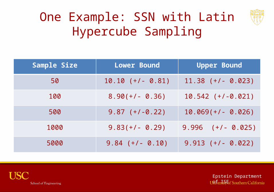
One Example: SSN with Latin Hypercube Sampling

Sample Size Lower Bound Upper Bound

50 10.10 (+/- 0.81) 11.38 (+/- 0.023)

100 8.90(+/- 0.36) 10.542 (+/-0.021)

500 9.87 (+/-0.22) 10.069(+/- 0.026)

1000 9.83(+/- 0.29) 9.996 (+/- 0.025)

5000 9.84 (+/- 0.10) 9.913 (+/- 0.022)


PC Configuration for SD

• Mac Book Air• Processor: Intel Core i5• Clock Speed: 1.8 GHz• 4 GB of 1600 MHz DDR3 Memory• Replications: 30 for each.


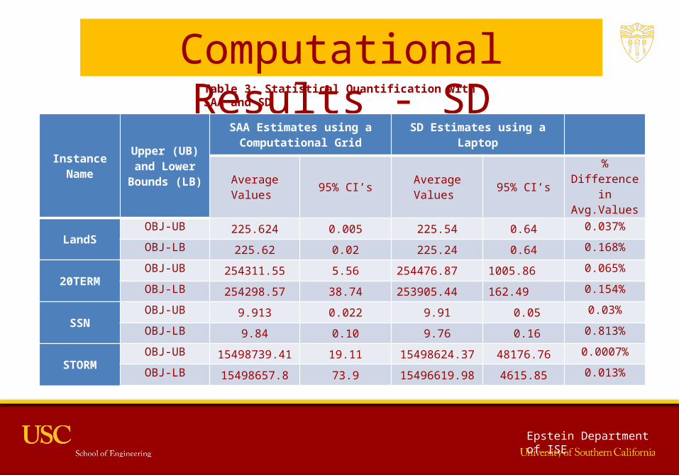
Computational Results - SD

Instance NameUpper (UB) and Lower Bounds

(LB)

SAA Estimates using a Computational Grid SD Estimates using a Laptop

Average Values 95% CI’s Average Values 95% CI’s

% Difference in Avg.Values

LandSOBJ-UB 225.624 0.005 225.54 0.64 0.037%

OBJ-LB 225.62 0.02 225.24 0.64 0.168%

20TERMOBJ-UB 254311.55 5.56 254476.87 1005.86 0.065%

OBJ-LB 254298.57 38.74 253905.44 162.49 0.154%

SSNOBJ-UB 9.913 0.022 9.91 0.05 0.03%

OBJ-LB 9.84 0.10 9.76 0.16 0.813%

STORMOBJ-UB 15498739.41 19.11 15498624.37 48176.76 0.0007%

OBJ-LB 15498657.8 73.9 15496619.98 4615.85 0.013%

Table 3: Statistical Quantification with SAA and SD


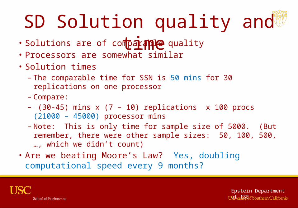
SD Solution quality and time • Solutions are of comparable quality• Processors are somewhat similar• Solution times

– The comparable time for SSN is 50 mins for 30 replications on one processor

– Compare: – (30-45) mins x (7 – 10) replications x 100 procs (21000 – 45000)

processor mins– Note: This is only time for sample size of 5000. (But remember, there

were other sample sizes: 50, 100, 500, …, which we didn’t count)• Are we beating Moore’s Law? Yes, doubling computational

speed every 9 months?


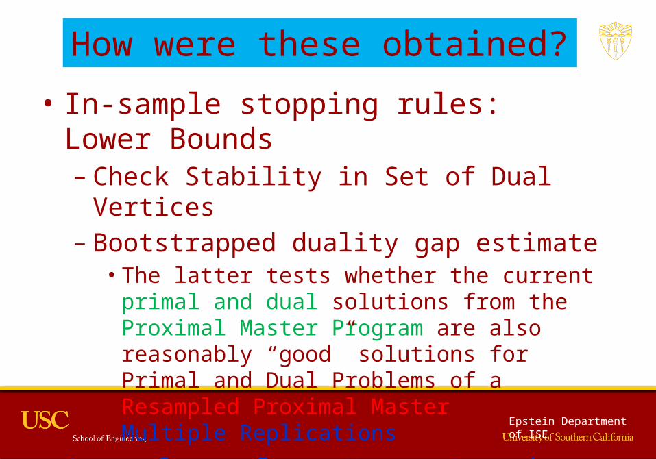
How were these obtained? • In-sample stopping rules: Lower Bounds

– Check Stability in Set of Dual Vertices– Bootstrapped duality gap estimate

• The latter tests whether the current primal and dual solutions from the Proximal Master Program are also reasonably “good” solutions for Primal and Dual Problems of a Resampled Proximal Master over Multiple Replications

• Out-of-sample: Upper Bounds


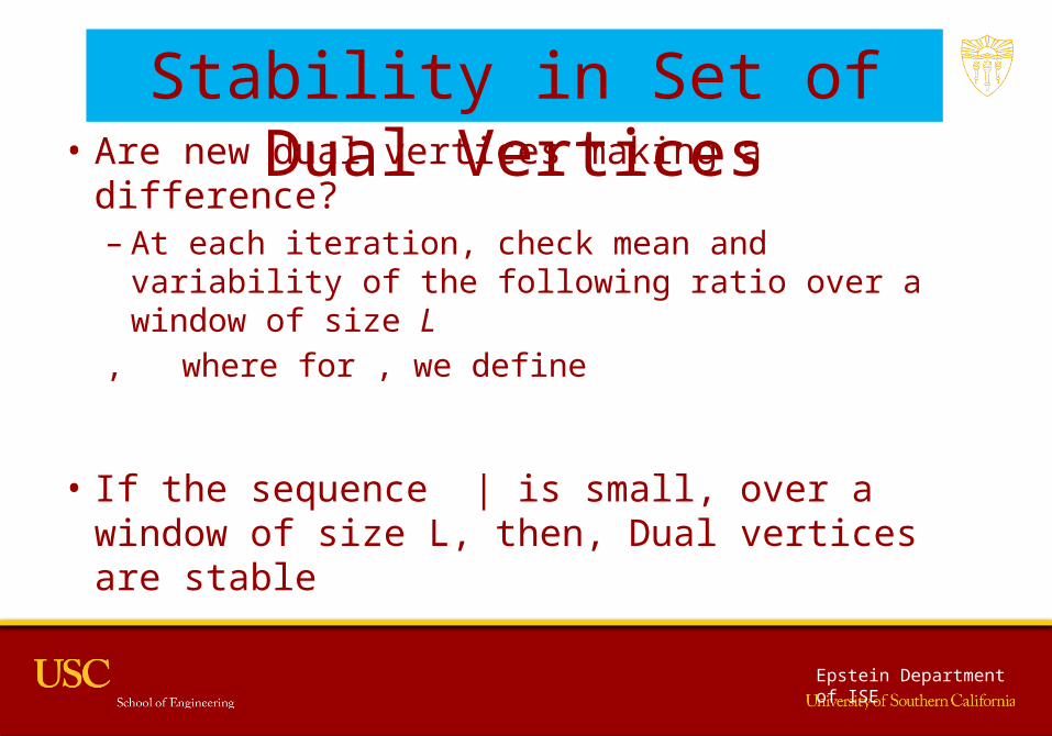
Stability in Set of Dual Vertices• Are new dual vertices making a difference?

– At each iteration, check mean and variability of the following ratio over a window of size L

, where for , we define

• If the sequence | is small, over a window of size L, then, Dual vertices are stable



Primal and Dual Regularized Values

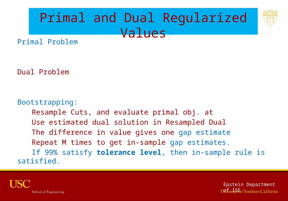
Primal Problem

Dual Problem

Bootstrapping: Resample Cuts, and evaluate primal obj. at

Use estimated dual solution in Resampled DualThe difference in value gives one gap estimateRepeat M times to get in-sample gap estimates. If 99% satisfy tolerance level, then in-sample rule is satisfied.


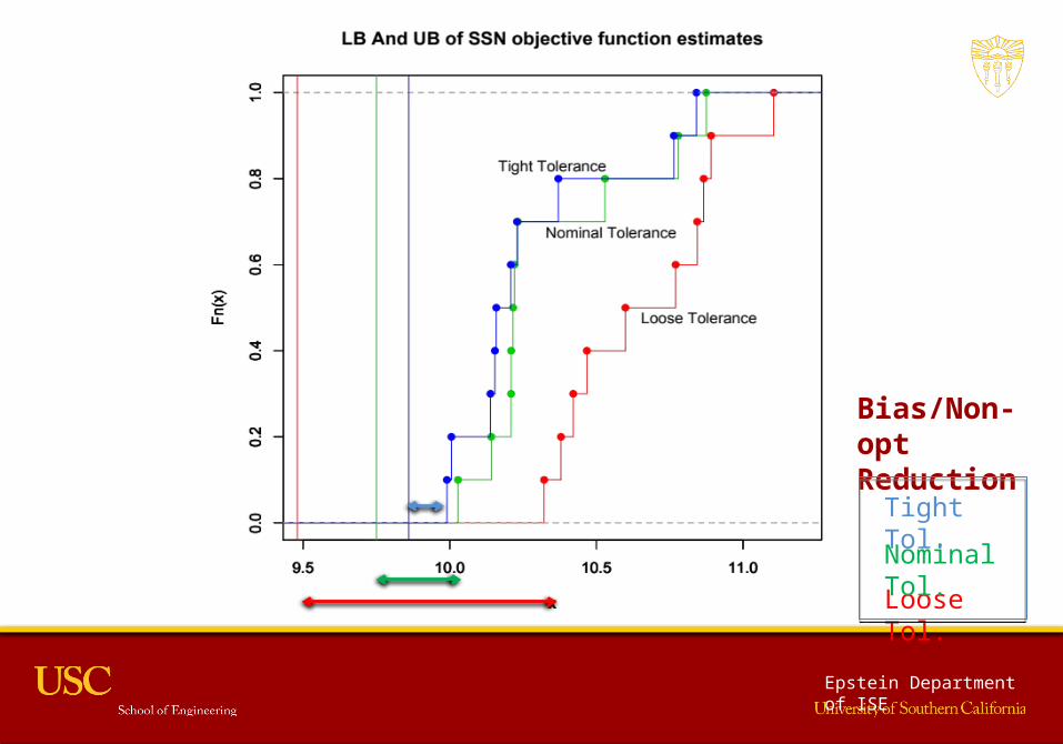
Loose Tol.

Nominal Tol.

Tight Tol.

Bias/Non-opt Reduction


SSN: Sonet-Switched NetworkSolution and evaluation time for 20’s replications (Tight)

Replication No. Solution Time (s) Evaluation Time (s)0 313.881051 588.6271841 203.690471 651.0422272 465.949416 547.5179963 313.606587 589.4298284 355.160629 599.3318085 334.764385 616.6748996 529.661100 604.5656307 327.888471 545.1320398 169.432233 655.6885309 301.293535 604.098964

10 697.304541 567.36143311 315.097318 532.59502612 247.439006 555.66437413 560.934417 577.25890014 342.787909 506.83677415 247.356803 570.57769016 184.941379 517.99921417 339.951593 589.26595818 339.381007 579.03326319 411.092300 602.349102

Total 7001.614151 11601.050839

Evaluation value ranges from 9.944203 to10.279154(3.3% difference)


Solutions

• Mean of Replications: Average all Solutions• For each seed s, let

where fs denotes the final approximation for seed s

• Compromise solution:


Upper Bounds

• For each replication, the objective function evaluations can be very time consuming

• We report Objective of both Mean and Compromise Solutions


Main Take Away

In SP,Numerical Optimization Meets Statistics

So When You Design Algorithms, Don’t Forget What You Need to Deliver: Statistics

Most Numerical Optimization Methods were Not Designed for This Goal.

• Does Speed-up with SD beat Moore’s Law? Yes, doubling computational speed every 9 months!

Sd4 tignes 2013-2

Documents

fk epstein department

byepstein department

stochastic program

kbl decomposition

master program

stage slp subgradients

algorithm difficult

early rounds