Screening of potential ecological risk of metal contamination ...

1

Research Journal of Physical and Applied Sciences 2013 Wudpecker Journals Vol. 2(4), pp. 052 - 063, August 2013

Screening of potential ecological risk of metal contamination in some Kenyan estuaries

Okuku EO1,2*, Ohowa B1, Ongore CO1, 3, Kiteresi LI1, Wanjeri VO1, Okumu S1 and Ochola O1

1Kenya Marine and Fisheries Research Institute, P.O. Box 81651, Mombasa, Kenya.

2Soil and Water Management Division, Faculty of Bioscience Engineering, Katholike Universiteit Leuven, Kasteelpark Arenberg 20, B-3001 Heverlee, Belgium.

3School of Environmental Studies (SES), Moi University, P.O. Box 3900, Eldoret, Kenya

*Corresponding author E-mail: [email protected] or [email protected] Telephone: +254 (020) 8021560/1, Fax: +254 (020) 2353226

Accepted 22 May 2013

Sediment core samples from seven stations in three Kenyan estuaries were analysed for Al, Ni, Zn, Cu, Cr, Mn and Pb by atomic absorption spectrophotometry to determine the spatial contamination (vertical and horizontal) and to identify any potential ecological risks. Samples were analysed for total metal concentration and data normalised using regression model of metal/Ni. The data was further compared to toxicity based Sediments Quality Guidelines (SQG) [Effects Range Low (ERL) and Effect Range Median (ERM)] giving an indication of potential ecological risks.There was a general reduction in metals input into the Kenya estuaries as evident from depletion of a number of metals in surface samples as compared to the subsurface samples. Enrichment Factors (EF) ranged from 0.1-92.9 indicating low to extreme contamination. Low contribution of anthropogenic sources of metal and the existence of metals in acceptable risk levels in most of the sites was also observed. However, some sites had a few samples with moderate to significant anthropogenic contribution of metals with the associated moderate to significant potential risk to biota. This study recommends a site-specific evaluation of these sites in order to quantify the level of risk, identifysource of contamination and suggest relevant management and mitigation measures. Keywords: Ecological risk, Kenyan estuaries, metals, marine pollution, sediments.

INTRODUCTION Developing countries have previously been considered as the least polluted. However, rapid industrial development and urbanization in these countries is gradually degrading coastal habitats, which are the final recipient of land-based pollutants (Huang and Lin, 2003; Kumar et al., 2010; Okuku et al., 2010). Metals are natural constituents of the marine environment. Their use in human history has yielded great benefits as well as harmful consequences. Historically, it has been the exploitation of the properties of metals which has led to successive waves of development of our modern technological society. However, metal pollution has been identifiedas a serious and widespread environmental problem due to their toxic, persistent, non-biodegradable and bio-accumulation properties (Yuan et al., 2004; Okuku et al., 2010; Okuku and Peter, 2012).

Rivers and streams are an important source and conduits for the transportation of anthropogenic metal to

the oceans (Everaarts and Nieuwenhuize, 1995; Adamo et al., 2005; Nicolau et al,. 2006). A significant amount of metal input to coastal zones ultimately accumulates in the estuarine zone and continental shelf which acts as important sinks for suspended matter and associated land-derived contaminants (Yeats and Bewers, 1983). Sources of estuarine metals include point and non-point upstream sources and from human habitations, tourism and industries, wastewater discharge and atmospheric deposition (Birth, 2003; Censi et al., 2006). Estuarine sediment contamination is currently receiving increased attention due to its recognition as a major source of ecosystem stress (Chapman and Wang, 2001; Riba et al., 2002).

Even though sediments are temporally and spatially heterogeneous in estuaries due to sedimentation and remobilization processes (Meybeck and Vörösmarty, 2005), sediments may encompass various temporal

2

053 Res. J. Phy. and Appl. Sci. storages and may in particular accumulate laterally and vertically in these systems (Bolviken et al., 2004; Provansal et al., 2010) thus enabling reconstruction of the pollution history over a long period of time (Bolviken et al., 2004; Meybeck et al., 2007; Le Cloarec et al., 2009).

Toxic metals in environmental and biological materials are increasingly demanded despite the fact it does not provide information on the mobility, bioavailability and toxicity of metals and may not be of direct biological significance (Ochieng et al., 2009; Okuku et al., 2010). For instance, total metal content is critical in assessing risk of contaminated sites; mapping hot spots areas; identification of anthropogenic inputs and it is alsocrucial for the purposes of ecological remediation and environment protection of estuarine wetlands(Huang and Lin, 2003).

Whereas some work on total metals have been carried out along the Kenyan Coast (Norconsult, 1977; Oteko, 1987; Wandiga and Onyari, 1987; Everaarts and Nieuwenhuize, 1995; Williams et al., 1996, Kamau, 2001; 2002; Okuku, 2010; 2012), there is currently no comprehensive information on metal vertical distribution as well as their potential ecological risks. The objective of this study was therefore to determine contamination levels and potential risks of copper, zinc, chromium, lead, manganese and aluminiumin sediment cores collected from some of the Kenyan estuaries. Core samples of formerly deposited sediments in the Kenyan estuaries were expected in this study to provide valuable information on pollution history. In order to assess the contamination degree of sediments and estimate their potential ecological risk, ERL and ERM (Long et al., 1995) were used as interpretive tools for relating ambient sediment chemistry data to the potential for adverse biological effects. These tools are some of the most widely used sediment quality guidelines for indicating the probable occurrence of biological effects when metal concentrations in sediment transcend reference values (O’Connor, 2004). The anthropogenic contribution of contamination in the estuaries was estimated through calculation of enrichment factors (Salomons and Forstner, 1984). MATERIALS AND METHODS Study area The sites sampled during this study were located in rivers the Tana, Sabaki and Ramisi estuaries (Figure 1). The Sabaki River originates from Ngong hills in central Kenya (as River Athi). It flows mainly through sand and rocks and mining industriesfor cement and other inorganic products as Athi River. It further flows through areas with major industries and coffee and tea farms where

agrochemicals and fertilizers are used in large scale before discharging into the Indian Ocean. Ramisi river estuary is located at Funzi Bay. The Ramisi River flows through Shimba Hills and later through an area extensively covered by different mangrove species before discharging into the Indian Ocean. The Tana River is the largest river in Kenya, arising on the south-western flank of Mount Kenya. With a drainage basin of 120,000 km2 (Ongwenyi et al., 1993), the Tana River flows for 1012 km and discharges into the Indian Ocean near Tana (Saha, 1982). Sample collection and analysis Three sediment cores were collected randomly at each location using plastic hand corers (diameter- 8 cm, length- 15 cm) and sectioned at intervals of 0 to 2, 2 to 4, 4 to 6, 6 to 9, 9 to 12 and 12-15 cm. The sediment for each section was pooled for each location and extraneous material (such as debris and stones) removed. The samples were mixed by hand and transported to the laboratory in cool boxes.

In the laboratory, sediment samples were freeze dried, homogenized and sieved through a 63 μm nylon sieve. The <63 μm fraction was kept in sealed plastic containers for analyses. The preference of <63 μm fraction is due to strong association of metals with fine-grained sediments (Tam and Wong, 2000). For the analysis, 0.25 g duplicate subsamples were weighed into teflon vessels and digested in 5ml HNO3 acid, 2ml H2O2 and 2ml HF by allowing it to stand at room temperatures for 12 hours and then decomposed in a microwave (Microwave accelerated Reaction system) at 1200W for 15 minutes. 80g of boric acid was added and the samples further decomposed for 45 minutes. The samples were qualitatively transferred into 50ml polyprothelene bottles and diluted with MilliQ water to 50 ml. For elemental analysis of Al, Cu, Zn, and Mn, a Varian SpectrAA 225 FS Atomic Absorption Spectrophotometer (AAS) was used whereas Pb and Cr were analysed using a Varian SpectrAA 220 FS AAS with Zeeman background correction. All the analyses were carried out at optimum instrument operating conditions recommended by the manufacturer.

Normal precautions for metals analysis were observed throughout, including the use of ultra-pure reagents and procedural blanks to check for contamination during sample preparation and analyses. In addition, quality of metal analyses was tested using estuarine sediment MESS 3 Certified Reference Material (Zech Metrological Institute) and check standards analysed after every 5 samples. Background correction and matrix interference were monitored throughout the analyses. Double de-ionized water from an integrated Millipore Milli-Q Academic and Milli-Q RiOs system (Millipore) was used

3

Okuku et al. 054

Figure 1. Map of sampling sites in some Kenyan estuaries.

for preparing the solutions and for dilutions. All the teflon vessels used for digestion were cleaned in the microwave using concentrated HNO3 and further cleaned in Trace Clean Automatic Cleaning Device for Ultra-Pure Chemistry (Milestone Microwave systems) and thoroughly rinsed with de-ionized water.

The analytical results of the selected metals of interest showed a good agreement between the reference and analytical values of the reference materials. The recovery rates for the analysed metals from the standard reference material were between 96% to 103%. The percentage moisture content for the samples were calculated and used to correct the results for moisture content. Normalization and enrichment factors calculations The use of non-normalised metals concentrations is increasingly criticized for evaluation of pollution status (Covelli and Fontolan, 1997) due to the fact that absolute concentration of metals in sediments does not necessarily indicate the degree of contamination. This is true considering that metals from natural and

anthropogenic sources may both accumulate in the sediments. Differences in sediment composition such as grain-size distribution and mineralogy have also been reported to affect metal concentrations (Loring, 1991). Furthermore, elevated metal concentration in sediments can also result from their geological material rather than contamination (Murray, 1996).

To compensate for natural variability of metals in sediment, geochemical approaches have been used to normalize the samples as well as to detect and quantify anthropogenic pollution (Summers et al., 1996; Covelli and Fontolan, 1997). This approach is based on a procedure that involves mathematical normalisation of metal concentrations to the concentrations of an elemental proxy for mineralogical as well as grain-size differences in sediments (Loring, 1991). Several methods of normalization have been applied, ranging from the use of simple metal/normalizer ratios to more complex methods based on regression analysis (Rowlatt and Lovell, 1994). Even though, there is no consensus about the most appropriate sediment constituent to be used for normalization, the most commonly used normalizers are Al (Sinex and Wright, 1988; Balls et al., 1997) and Fe

4

055 Res. J. Phy. and Appl. Sci.

Table 1. Correlation matrix of metals in Kenyan Estuarine sediments.

Al Ni Zn Cu Cr Mn Pb Al 1 Ni -0.20 1 Zn -0.11 0.96* 1 Cu -0.15 0.97* 1.00* 1 Cr -0.12 0.93* 0.99* 0.99* 1 Mn 0.87* 0.27 0.38 0.35 0.36 1 Pb -0.11 0.89* 0.98* 0.97* 0.99* 0.38 1

* Correlations significant at <0.001

Table 2. Metal/ Ni Regression model results for metals in selected sites in Kenyan estuaries.

Metal R2 P Slope Intercept Zn 0.842 <0.001 2.77 10.70 Cu 0.909 <0.001 1.32 -0.296 Cr 0.718 <0.001 1.71 18.54 Mn 0.042 >0.05 36.91 2030 Pb 0.546 <0.001 1.12 -8.15 Al 0.002 >0.05 -3241 1136649

(Ackerman, 1980; Emmerson et al., 1997). However, the distribution of these metals in the Kenyan estuarine sediments showed some evidence of anthropogenic enrichment and Ni was found to be the most suitable normalizer based on significant correlation and linear regression trends observed between Ni and most metals (Table 1 and 2).

In this study, regression analysis of Metal/Ni was used to geochemically normalize the dataset and to simultaneously allow for establishment of mathematical geochemical backgrounds. The formula below was applied to calculate indicative enrichment factors (EF) once the background levels were established (Covelli and Fontolan, 1997). In this formula, EF was defined as the ratio between the real and predicted values, where the predicted value is within the range of 1 ±2σ) EF = (Xsample/normalizing agent)/(Xpredicted/normalizing agent) Where: Xsample is the concentration of the element of interest Xpredicted is the predicted concentration of the element of interest. RESULTS AND DISCUSSION Distribution of metals in Kenyan estuaries Mean total metal concentrations in sediment cores are

presented in Tables 3, 4 and 5. Spatial variation of metal concentration in surface sediments could be attributed to mixing of sediments from different origins and to differences in pollution sources (Förstner, 1981). Sediment in Ramisi Upper had higher concentrations of Pb, Zn, Cu, Mn and Cr as compared to sedimentin the mid part of Ramisi. Tana River’s Tana village station had the highest metal concentration among all the study sites sampled except for Al (Tables 3, 4 and 5). Worth noting is the very high concentrations of Pb in Tana Village. Pb in estuaries originate mostly from battery casings and plates (WHO, 1989) or petrol deposits resulting from the use of leaded gasoline in vessels and motor vehicles, from atmospheric deposition (Liu et al., 2003) and accidental spillage. Metal concentration was also relatively high in Sabaki Bridge. This could be attributed to atmospheric deposition, road wear, tire wear and vehicle wear which have been identified as major contributors of metals to the aquatic ecosystem (Taylor, 2007). Generally, Tana Village of Tana River estuary had the highest concentration of metals (Tables 3 and 5) in the surface sediments.

Cr concentrations in the sites were higher than those of Dipsiz stream (mean of 19.70µg/g) and Naples Harbour, (21.6 ± 6.9µg/g) as shown in Table 6. High concentration of Cr could be attributed to intensive chemical weathering of source rock in tropical environments (Nagender et al., 2000). The mean Cu sediment concentration was comparable to those reported for Keelung river (range 12-110µg/g ) but higher than the concentrations reported for Yamuna River (mean of 22.2µg/g) Ebro stream

5

Okuku et al. 056

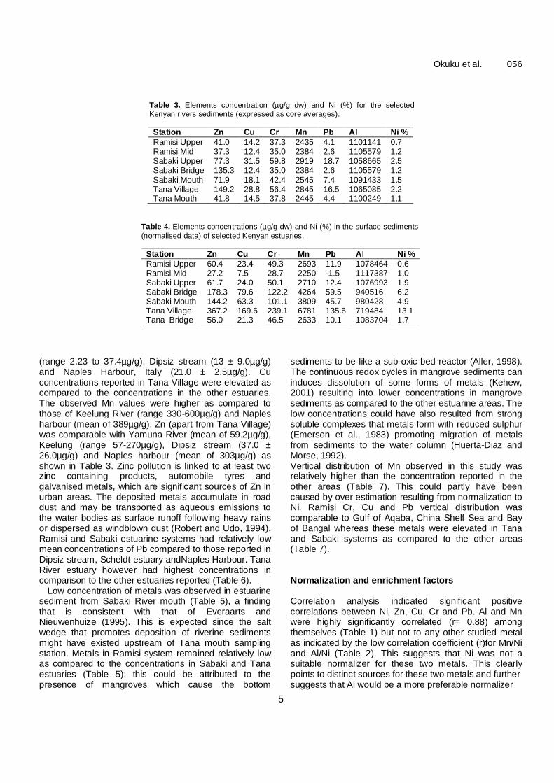
Table 3. Elements concentration (µg/g dw) and Ni (%) for the selected Kenyan rivers sediments (expressed as core averages). Station Zn Cu Cr Mn Pb Al Ni % Ramisi Upper 41.0 14.2 37.3 2435 4.1 1101141 0.7 Ramisi Mid 37.3 12.4 35.0 2384 2.6 1105579 1.2 Sabaki Upper 77.3 31.5 59.8 2919 18.7 1058665 2.5 Sabaki Bridge 135.3 12.4 35.0 2384 2.6 1105579 1.2 Sabaki Mouth 71.9 18.1 42.4 2545 7.4 1091433 1.5 Tana Village 149.2 28.8 56.4 2845 16.5 1065085 2.2 Tana Mouth 41.8 14.5 37.8 2445 4.4 1100249 1.1

Table 4. Elements concentrations (µg/g dw) and Ni (%) in the surface sediments (normalised data) of selected Kenyan estuaries.

Station Zn Cu Cr Mn Pb Al Ni % Ramisi Upper 60.4 23.4 49.3 2693 11.9 1078464 0.6 Ramisi Mid 27.2 7.5 28.7 2250 -1.5 1117387 1.0 Sabaki Upper 61.7 24.0 50.1 2710 12.4 1076993 1.9 Sabaki Bridge 178.3 79.6 122.2 4264 59.5 940516 6.2 Sabaki Mouth 144.2 63.3 101.1 3809 45.7 980428 4.9 Tana Village 367.2 169.6 239.1 6781 135.6 719484 13.1 Tana Bridge 56.0 21.3 46.5 2633 10.1 1083704 1.7

(range 2.23 to 37.4µg/g), Dipsiz stream (13 ± 9.0µg/g) and Naples Harbour, Italy (21.0 ± 2.5µg/g). Cu concentrations reported in Tana Village were elevated as compared to the concentrations in the other estuaries. The observed Mn values were higher as compared to those of Keelung River (range 330-600µg/g) and Naples harbour (mean of 389µg/g). Zn (apart from Tana Village) was comparable with Yamuna River (mean of 59.2µg/g), Keelung (range 57-270µg/g), Dipsiz stream (37.0 ± 26.0µg/g) and Naples harbour (mean of 303µg/g) as shown in Table 3. Zinc pollution is linked to at least two zinc containing products, automobile tyres and galvanised metals, which are significant sources of Zn in urban areas. The deposited metals accumulate in road dust and may be transported as aqueous emissions to the water bodies as surface runoff following heavy rains or dispersed as windblown dust (Robert and Udo, 1994). Ramisi and Sabaki estuarine systems had relatively low mean concentrations of Pb compared to those reported in Dipsiz stream, Scheldt estuary andNaples Harbour. Tana River estuary however had highest concentrations in comparison to the other estuaries reported (Table 6).

Low concentration of metals was observed in estuarine sediment from Sabaki River mouth (Table 5), a finding that is consistent with that of Everaarts and Nieuwenhuize (1995). This is expected since the salt wedge that promotes deposition of riverine sediments might have existed upstream of Tana mouth sampling station. Metals in Ramisi system remained relatively low as compared to the concentrations in Sabaki and Tana estuaries (Table 5); this could be attributed to the presence of mangroves which cause the bottom

sediments to be like a sub-oxic bed reactor (Aller, 1998). The continuous redox cycles in mangrove sediments can induces dissolution of some forms of metals (Kehew, 2001) resulting into lower concentrations in mangrove sediments as compared to the other estuarine areas. The low concentrations could have also resulted from strong soluble complexes that metals form with reduced sulphur (Emerson et al., 1983) promoting migration of metals from sediments to the water column (Huerta-Diaz and Morse, 1992). Vertical distribution of Mn observed in this study was relatively higher than the concentration reported in the other areas (Table 7). This could partly have been caused by over estimation resulting from normalization to Ni. Ramisi Cr, Cu and Pb vertical distribution was comparable to Gulf of Aqaba, China Shelf Sea and Bay of Bangal whereas these metals were elevated in Tana and Sabaki systems as compared to the other areas (Table 7). Normalization and enrichment factors Correlation analysis indicated significant positive correlations between Ni, Zn, Cu, Cr and Pb. Al and Mn were highly significantly correlated (r= 0.88) among themselves (Table 1) but not to any other studied metal as indicated by the low correlation coefficient (r)for Mn/Ni and Al/Ni (Table 2). This suggests that Ni was not a suitable normalizer for these two metals. This clearly points to distinct sources for these two metals and further suggests that Al would be a more preferable normalizer

6

057 Res. J. Phy. and Appl. Sci. Table 5a. The observed and predicted (based on regression normalisation to Ni) metals concentration (in µg/g except Ni in %) in selected sites in Kenyan major estuaries.

Site Core depth

Zn Cu Cr Mn Pb Al Ni (%) Observed Predi

cted Observed Predicted Observed Predicted Observed Predicted Observed Predicted Observed Predicted

Ramisi Upper 0-2 55.9 60.4 20.6 23.4 62.5 49.3 383.6 2693.1 18.6 11.9 85104 1078464 0.6 Ramisi Upper 2-4 40.9 42.9 14.9 15.1 47.1 38.5 173.3 2460.0 14.9 4.8 68131 1098937 0.6 Ramisi Upper 4-6 28.8 19.8 11.8 4.0 34.8 24.2 105.2 2151.5 11.2 -4.5 53351 1126023 0.8 Ramisi Mid 0-2 36.8 27.2 14.3 7.5 41.3 28.7 1035.2 2249.9 14.6 -1.5 63525 1117387 1.0 Ramisi Mid 2-4 30.7 27.0 12.8 7.5 39.1 28.6 813.2 2247.4 14.5 -1.6 60418 1117604 1.2 Ramisi Mid 4-6 34.5 31.9 14.0 9.8 41.4 31.6 575.8 2312.3 35.4 0.4 62004 1111900 1.7 Ramisi Mid 6-9 37.7 36.6 15.0 12.0 44.0 34.6 165.0 2375.5 14.3 2.3 66593 1106352 1.8 Ramisi Mid 9-12 47.0 44.0 18.3 15.6 50.0 39.2 220.3 2474.7 15.4 5.3 75755 1097643 1.2 Ramisi Mid 12-15 58.6 56.9 21.6 21.7 60.6 47.1 322.9 2646.1 16.2 10.5 88140 1082587 0.3 Sabaki Upper 0-2 65.8 61.7 24.3 24.0 53.7 50.1 766.6 2709.8 17.8 12.4 92992 1076993 1.9 Sabaki Upper 2-4 87.0 91.5 34.5 38.2 61.2 68.5 779.3 3106.8 17.1 24.4 94323 1042129 3.0 Sabaki Upper 4-6 83.6 87.8 36.5 36.5 61.8 66.3 1000.5 3058.4 18.7 23.0 105386 1046384 2.8 Sabaki Upper 6-9 70.0 64.6 26.6 25.4 61.0 51.9 844.9 2748.1 17.6 13.6 95130 1073630 2.0 Sabaki Upper 9-12 58.5 61.1 21.0 23.7 51.4 49.7 756.8 2702.4 19.5 12.2 96072 1077644 1.9 Sabaki Upper 12-15 85.6 97.4 44.8 41.0 68.1 72.2 1069.8 3185.6 19.5 26.8 100700 1035211 3.2 Sabaki Bridge 0-2 122.2 178.3 63.4 79.6 81.3 122.2 1367.7 4263.9 17.8 59.5 129699 940516 6.2 Sabaki Bridge 2-4 77.7 85.9 31.9 35.5 61.7 65.0 869.6 3031.8 19.0 22.2 101485 1048717 2.8 Sabaki Bridge 4-6 115.0 147.8 53.5 65.0 57.0 103.3 1017.6 3857.1 13.5 47.1 109623 976240 5.0 Sabaki Bridge 6-9 98.8 122.1 43.9 52.8 64.2 87.4 1083.7 3514.7 13.7 36.8 106520 1006312 4.1 Sabaki Bridge 9-12 101.1 142.2 46.2 62.4 58.3 99.9 1113.2 3783.0 13.3 44.9 113019 982754 4.8 Sabaki Bridge 12-15 97.4 135.4 43.7 59.1 52.5 95.7 1069.3 3691.4 12.8 42.1 103738 990790 4.6 Sabaki Mouth 0-2 93.7 144.2 44.2 63.3 58.3 101.1 1286.7 3809.4 14.4 45.7 105021 980428 4.9

for Mn compared to Ni.

The statistical methodology applied during normalization resulted into highly significant regressions (p< 0.001) of most metals with Ni (Table 2). The model showed a good agreement between predicted and observed values, with predictedconcentrations generally falling within the 95% confidence interval. The exception was Mn and Al in which the model demonstrated a tendency of over predicting the concentrations. Al and Mn were therefore not considered for calculations of EF and in risk assessment. Even though it has been argued elsewhere that the ratios of metal/Al are usually fairly constant in

the earth’s crust (Kersten and Smedes, 2002) and possess an added advantage over the traditional granulometric approaches in identifying technogenic enhancements and comparison between samples (Kersten and Smedes, 2002), Al in the present study was found to be less robust (as compared to Ni) with metal/Al relationship that were not significant except with Mn. Metal/Ni regression model used showed (through the negative values of the EFs) that a few samples in Ramisi and Tana estuaries were depleted in Pb (Table 5). In this case predicted values were higher than the observed concentrations, which consistently points to a

depletion of the used geochemical tracer (Ni).The enrichment factors of most samples oscillated close to 1, reflecting baseline conditions and a range of natural variability (Table 8). In spite of the large variations in grain size and environmental conditions in the Kenyan estuaries, the significant regression for most metals show that the metals behaved according to the variability of Ni grain size proxy, suggesting that Ni is a suitable reference tool for the recognition of anthropogenic inputs. This study has further proved the usefulnessof regression analysis for normalizing geochemical data, as well as in discerning between natural and anthropogenic enrichments,

7

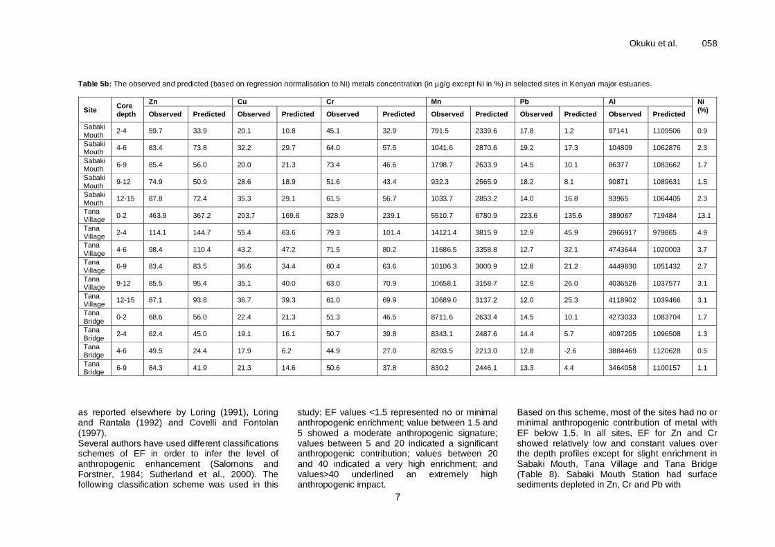
Okuku et al. 058 Table 5b: The observed and predicted (based on regression normalisation to Ni) metals concentration (in µg/g except Ni in %) in selected sites in Kenyan major estuaries.

Site Core depth

Zn Cu Cr Mn Pb Al Ni (%) Observed Predicted Observed Predicted Observed Predicted Observed Predicted Observed Predicted Observed Predicted

Sabaki Mouth 2-4 59.7 33.9 20.1 10.8 45.1 32.9 791.5 2339.6 17.8 1.2 97141 1109506 0.9

Sabaki Mouth 4-6 83.4 73.8 32.2 29.7 64.0 57.5 1041.6 2870.6 19.2 17.3 104809 1062876 2.3

Sabaki Mouth 6-9 85.4 56.0 20.0 21.3 73.4 46.6 1798.7 2633.9 14.5 10.1 86377 1083662 1.7

Sabaki Mouth 9-12 74.9 50.9 28.6 18.9 51.6 43.4 932.3 2565.9 18.2 8.1 90871 1089631 1.5

Sabaki Mouth 12-15 87.8 72.4 35.3 29.1 61.5 56.7 1033.7 2853.2 14.0 16.8 93965 1064405 2.3

Tana Village 0-2 463.9 367.2 203.7 169.6 328.9 239.1 5510.7 6780.9 223.6 135.6 389067 719484 13.1

Tana Village 2-4 114.1 144.7 55.4 63.6 79.3 101.4 14121.4 3815.9 12.9 45.9 2966917 979865 4.9

Tana Village 4-6 98.4 110.4 43.2 47.2 71.5 80.2 11686.5 3358.8 12.7 32.1 4743644 1020003 3.7

Tana Village 6-9 83.4 83.5 36.6 34.4 60.4 63.6 10106.3 3000.9 12.8 21.2 4449830 1051432 2.7

Tana Village 9-12 85.5 95.4 35.1 40.0 63.0 70.9 10658.1 3158.7 12.9 26.0 4036526 1037577 3.1

Tana Village 12-15 87.1 93.8 36.7 39.3 61.0 69.9 10689.0 3137.2 12.0 25.3 4118902 1039466 3.1

Tana Bridge 0-2 68.6 56.0 22.4 21.3 51.3 46.5 8711.6 2633.4 14.5 10.1 4273033 1083704 1.7

Tana Bridge 2-4 62.4 45.0 19.1 16.1 50.7 39.8 8343.1 2487.6 14.4 5.7 4097205 1096508 1.3

Tana Bridge 4-6 49.5 24.4 17.9 6.2 44.9 27.0 8293.5 2213.0 12.8 -2.6 3884469 1120628 0.5

Tana Bridge 6-9 84.3 41.9 21.3 14.6 50.6 37.8 830.2 2446.1 13.3 4.4 3464058 1100157 1.1

as reported elsewhere by Loring (1991), Loring and Rantala (1992) and Covelli and Fontolan (1997). Several authors have used different classifications schemes of EF in order to infer the level of anthropogenic enhancement (Salomons and Forstner, 1984; Sutherland et al., 2000). The following classification scheme was used in this

study: EF values <1.5 represented no or minimal anthropogenic enrichment; value between 1.5 and 5 showed a moderate anthropogenic signature; values between 5 and 20 indicated a significant anthropogenic contribution; values between 20 and 40 indicated a very high enrichment; and values>40 underlined an extremely high anthropogenic impact.

Based on this scheme, most of the sites had no or minimal anthropogenic contribution of metal with EF below 1.5. In all sites, EF for Zn and Cr showed relatively low and constant values over the depth profiles except for slight enrichment in Sabaki Mouth, Tana Village and Tana Bridge (Table 8). Sabaki Mouth Station had surface sediments depleted in Zn, Cr and Pb with

8

059 Res. J. Phy. and Appl. Sci.

Table 6. Comparison of elements concentration of surface sediments in selected systems in the world. Estuary Ni Zn Cu Cr Mn Pb Reference Dipsiz Stream, Turkey - - 13 ± 9.0 19.7 - 83.6 ±56.2 Adamo et al. 2005 Naples Habour, Italy - 389 - 21.6 ± 6.9 - 131 Demirak et al. 2006 Yamuna River - 59.2 22.2 - - 60.3 Jain 2004 Keelung River - 330-600 12-110 - - - Huang and Lin 2003 Tigris River, Turkey - 89-716 641-3433 - - 24-102 Gumgum et al. 1994 South Plate River, USA - 82-3700 18-480 - - 19-270 Heiny and Tate 1997

Ebro River - 20.6-198.5 2.23-37.4 - - 2.82-69.7 Ramos et al.1999 Adyar estuary 18 -38 60-168 - 225-318 244-569 2-11 Achyuthanet al.2002 Scheldt Estuary 14.7±5.1 263±98 48±19 - - 93±36 Baeyens et al. 2005 Ramisi 5.94-18.0 27.2-60.4 7.5-23.4 28.7-49.3 2250-2693 -1.5-11.9 This study Sabaki 8.37-60.5 61.7-178.3 24.0-79.6 50.1-101.1 2710-4264 12.4-59.5 This study Tana 16.3-128.7 56.0-367.2 21.3-169.6 46.5-239.1 2633-6781 10.1-135.6 This study

Table 7. Comparison of elements concentration of core sediments in selected systems in the world.

System Mn Cr Cu Pb Reference Gulf of Aqaba 53-655 15-655 7-27 83-225 Abu-Hilal 1987 China Shelf Sea 530 61 15 17 Yiyang and Ming-cai 1992 Gulf of St. Lawrence 700 87 25 21 Loring 1978; 1979 Bay of Bangal 529 84 26 - Sarine et al. 1979 Ramisi 2151-2693 24.2-49.3 4.0-23.4 -4.5-11.9 This study Tana 2213-6780 27.0-239.1 6.2-169.6 -2.6-135.6 This study Sabaki 2339-4264 32.9-122.2 18.9-79.6 1.2-47.1 This study

enrichment in the 2 to 4cm depth (EF 1.8 to 14.8) an indication of reduced recent inputs of these metals in the stations.

Tana Bridge had 31% of the samples enriched in the various metals (EF between 2 and 3.0) indicative of moderate anthropogenic inputs of metal in this station. However, it is worth noting that for Zn, Cr, and Cu, enrichment was only observed in the depth profile 4-6cm and not in the top 4cm sediments. This could be an indication of past deposition of these metals with substantial decrease in the inputs in the recent past.

In general, 4 to 43% of the samples from Tana Bridge, Tana village, Sabaki Mouth and Ramisi Mid sites had EF of 1.5 to 5 showing that these sites had moderate anthropogenic input of metals in the order of Pb>Cu>Zn>Cr (Table 5). Only Pb in Sabaki Mouth Station (depth 2-4cm) and Ramisi Mid station (depth 6-9cm) had EF of 5-20 suggesting that these stations had significant anthropogenic contributions of Pb. Only Ramisi upper station (depth 4-6cm) that had EF above 40 indicating that this station had extremely high anthropogenic inputs of Pb. Pb enrichment in Ramisi station is not surprising given the existence of Ramisi Sugar Company that might have been a source of this metal. It is however important to note that the observed Pb enrichment was only in the subsurface samples and not in surface samples, an indication of reduced Pb input

in the recent past resulting from the ban on importation and use of leaded fuel. The high concentrations of Pb in 4 to 6 cm might have also coincided with the period when the sugar factory was in operation before it later stalled. Risk assessment of metals in Kenya estuaries Contaminated sediments do not only serve as diffuse source of contamination to the overlying water by slowly releasing the contaminant back into the water column (DEC, 1989; Marcus, 1991) but also pose a direct risk to the resident detrital and deposit-feeding benthic organisms (Mendil and Uluözlü, 2007). Organisms living in the sediments are in constant contact with the sediments with the associated contaminants that may be adsorbed to the sediment particles. Potential impacts of contaminated sediments to benthic organisms include both acute and chronic toxicity with individual-, population-, and community- level effects, bioaccumulation of contaminants and the potential to pass contaminants along to predators of benthic species (Marcus, 1991; Adams et al., 1992). Chemistry, toxicity and bioaccumulation tests are frequently used to evaluate risks of contaminated sediments to environmental receptors (USEPA, 2005). Whereas chemistry measurements can provide quantitative

9

Okuku et al. 060

Table 8. Enrichment Factors of metals in Kenya major estuaries’ sediments.

Site Depth Zn Cu Cr Pb Ramisi Upper 0-2 1.4 1.9 1.4 -9.7 Ramisi Upper 2-4 1.1 1.7 1.4 -9.1 Ramisi Upper 4-6 1.1 1.4 1.3 92.9 Ramisi Mid 0-2 0.9 0.9 1.3 1.6 Ramisi Mid 2-4 1.0 1.0 1.2 3.1 Ramisi Mid 4-6 1.5 2.9 1.4 -2.5 Ramisi Mid 6-9 1.0 1.2 1.3 6.2 Ramisi Mid 9-12 1.1 1.2 1.3 2.9 Ramisi Mid 12-15 1.0 1.0 1.3 1.5 Sabaki Upper 0-2 1.1 1.0 1.1 1.4 Sabaki Upper 2-4 1.0 0.9 0.9 0.7 Sabaki Upper 4-6 1.0 1.0 0.9 0.8 Sabaki Upper 6-9 1.1 1.0 1.2 1.3 Sabaki Upper 9-12 1.0 0.9 1.0 1.6 Sabaki Upper 12-15 0.9 1.1 0.9 0.7 Sabaki Bridge 0-2 0.7 0.8 0.7 0.3 Sabaki Bridge 2-4 0.9 0.9 0.9 0.9 Sabaki Bridge 4-6 0.8 0.8 0.6 0.3 Sabaki Bridge 6-9 0.8 0.8 0.7 0.4 Sabaki Bridge 9-12 0.7 0.7 0.6 0.3 Sabaki Bridge 12-15 0.7 0.7 0.5 0.3 Sabaki Mouth 0-2 0.6 0.7 0.6 0.3 Sabaki Mouth 2-4 1.8 1.9 1.4 14.8 Sabaki Mouth 4-6 1.1 1.1 1.1 1.1 Sabaki Mouth 6-9 1.5 0.9 1.6 1.4 Sabaki Mouth 9-12 1.5 1.5 1.2 2.3 Sabaki Mouth 12-15 1.2 1.2 1.1 0.8 Tana Village 0-2 1.3 1.2 1.4 1.6 Tana Village 4-6 0.8 0.9 0.8 0.3 Tana Village 6-9 0.9 0.9 0.9 0.4 Tana Village 9-12 1.0 1.1 0.9 0.6 Tana Village 12-15 0.9 0.9 0.9 0.5 Tana Village 15-18 0.9 0.9 0.9 0.5 Tana Bridge 0-2 1.2 1.1 1.1 1.4 Tana Bridge 2-4 1.4 1.2 1.3 2.5 Tana Bridge 4-6 2.0 2.9 1.7 -4.9 Tana Bridge 6-9 2.0 1.5 1.3 3.0

information on contaminants, toxicity tests provides direct measures of biological impacts (ASTM, 2009).A combination of these approaches through comparison of chemistry data to toxicity effect-based sediment quality guidelines can be used to evaluate the severity of sediment contamination (Wenning et al., 2005).

The ERL for Cr, Cu, Pb, and Zn in the scheme proposed by MacDonald et al. (2000) are 80, 70, 35, and 120µg/g whereas ERM for Cr, Cu, Pb, and Zn are 145, 390, 110, and 270µg/g. Based on this scheme, 43%, 29%, 57% and 86% of surface samples and 97%, 57%, 83% and 93%of the subsurface samples had concentrations below ERL for Zn, Cu, Cr and Pb respectively. This indicates that the effects of metals in the sediments are of acceptable levels. 14%, 43%, and 29% of the surface samples and 3.3%, 43%, and 17% of the subsurface samples had metal

concentrations above ERL but below ERM for Zn, Cu and Cr respectively. This is indicative of sediments contamination with moderate impacts to benthic life (i.e. concentration of Zn, Cu and Cr contamination in the sediment can be tolerated by majority of benthic organisms with toxicity only occurring to a few species). Only 14% of the surface samples had Zn, Pb and Cr concentrations above EMR, an indication that the sedimentsare contaminated and significant harm to benthic aquatic life is anticipated. None of subsurface samples had metal concentrations above EMR. Conclusion and recommendations 1. EFs have proved to be a useful tool in comparing Kenyan estuaries with various compositions and in

10

061 Res. J. Phy. and Appl. Sci. evaluating the extent of the historical metal pollution as well as in estimating the anthropogenic contribution of trace element.Whereas most of the sites had metals in acceptable levels, 17% of samples had moderate anthropogenic contribution of Zn, Cu, Cr, and Pb while only 1.4% of the samples had significant toextremely high anthropogenic contribution of Pb. There is therefore an urgent need for critical evaluation of the actual sources of metals in these 1.4% samples. 2. Even though most stations showed reduction in the concentrations of metals in the recent past, some stations such as Tana Village (Pb), Tana Bridge (Mn and Al) and Ramisi Upper (Cu) has experienced a slight increase in the concentration of the respective metal in the recent past and as such appropriate actions should be taken including identification of the sources and enforcement of environmental protection legislation including polluter pays principle to protect these sensitive ecosystems from adverse ecological disasters. 3. ERL and ERM SQGs were successfully applied in Kenya estuarine sediments for screening purposes in order to identify potentially contaminated sites and to provide a qualitative estimate of risk. Based on these tools, Tana Village surface sediment was found to be contaminated by Zn, Pb and Cr and significant harm to benthic aquatic life is anticipated. This study recommends a site-specific evaluation (i.e. additional chemical testing; sediment toxicity testing; or sediment bioaccumulation tests) to quantify the level of risk, determine if remediation actions are necessary and where necessary, come up with appropriate risk management actions. Acknowledgement Funding for this work was provided by SEED funds (Kenya Marine and Fisheries Research Institute, KMFRI) and RAF 7008 Project (International Atomic Energy Agency, IAEA). We are greatly indebted to the Directors of these institutions for supporting this work. We also appreciate the efforts of KMFRI and IAEA-Monaco staff that assisted in one way or another in fieldwork and laboratory analysis. We also acknowledge the efforts of the anonymous reviewer who tirelessly and promptly critiqued this work. REFERENCES Abu-Hilal AH (1987). Distribution of trace elements in

near shore surface sediments from the Jordan Gulf of Agaba (Red Sea). Mar. Poll. Bull., 18: 190-193.

Achyuthan H, Richardmohan D, Srinivasalu S, Selvaraj K (2002). Trace metals concentration in sediments cores of estuary and Tidal zones between Chennai and

Pondicheri along east coast of India. Indian J. Mar. Sci.,

31: 141-149. Ackerman F (1980). A procedure for correcting the grain

size effect in heavy metal analyses of estuarine and coastal sediments. Environ. Technol. Lett., 1:518-527.

ASTM (2009).Standard test methods for measuring the toxicity of sediment-associated contaminants with freshwater invertebrates. In: Annual book of ASTM standards, E1706-05, vol 11.06. ASTM, West Conshohocken, PA, 11(6): 947–1063.

Adamo P, Arienzo M, Imperato M, Naimo D, Nardi G, Stanzione D (2005). Distribution and partition of heavy metals in surface and sub-surface sediments of Naples city port. Chemos. 61: 800-809.

Adams WJ, Kimerle RA, Barnett Jr.JW (1992). Sediment Quality and Aquatic Life Assessment. Environ. Sci. Technol., 26: 1865-1875.

Aller RC (1998). Mobile deltaic and continental shelf muds as suboxic, fluidized bed reactors. Mar. Chem., 61: 143-155.

Baeyens W, Leermakers M, De Gieter M, Nguyen HL, Parmentier K, Panutrakul S, Elskens M (2005). Overview of trace metal contamination in the Scheldt estuary and effect of regulatory measures. Hydrobiologia, 540: 141-154.

Balls PW, Hull S, Miller BS, Pirie JM, Proctor W (1997). Trace metal in Scottish Estuarine and coastal sediments. Mar. Poll. Bull., 34: 42-50.

Birth G (2003). A scheme for assessing human impacts on coastal aquatic environments using sediments. In: Woodcoffe CD, Furness RA (eds) Coastal GIS 2003. Wollongong University Papers in Center for Maritime Policy, 14, Australia.

Bolviken B, Bogen J, Jartun M, Langedal M, Ottesen RT, Volden T (2004). Overbank sediments: A natural blending sampling medium for large-scale geochemical mapping. Chemometr. Intell. Lab. 74: 183-199.

Censi P, Spoto SE, Saino F, Sprovieri M, Mazzola S, Nardone DGG, Punturo SI, Ottonello D (2006). Heavy metals in coastal water systems: A case study from the northwestern Gulf of Thailand. Chemosphere, 64: 1167-1176.

Chapman PM, Wang F (2001). Assessing sediment contamination in estuaries. Environ. Toxicol. Chem., 20: 3-22.

Covelli S, Fontolan G (1997). Application of a normalization procedure in determining regional geochemical baselines. Environ. Geol., 30: 34–45.

DEC (1989). Non-point Source Assessment Report. New York Department of Environmental Conservation, Division of Water, Bureau of Water Quality Management.

Demirak A, Yilmaz F, Tuna AL, Ozdemir N (2006). Heavy metals in water, sediment and tissues of Leuciscuscephalus from a stream in south western Turkey. Chemos., 63: 1451-1458.

11

Emerson S, Jacobs L, Tebo B (1983). Behaviour of trace

metals in anoxic waters: solubilities at the oxygen-hydrogen sulfide interface. In: Wong CS, Boyle E, Bruland KW, Burton JD, Goldberg ED (eds) Trace Metals in Seawater. Plenum Press, New York and London. pp 579-608.

Emmerson RHC, O'Reilly-Wiese SB, Macleod CL, Lester JN (1997). A multivariate assessment of metal distribution in inter-tidal sediments of the Blackwater Estuary, UK. Mar. Poll. Bull. 34: 960-968.

Everaarts JM, Nieuwenhuize J (1995). Heavy metals in surface sediments and epibenthic macro invertebrates from the coastal zone and continental slope of Kenya. Mar. Poll. Bull. 31: 281-289.

Förstner U (1981). Metal transfer between solid and aqueous phases. In: Förtner U, Wittmann GTW (eds) Metal pollution in the aquatic environment. Berlin-Heidelberg, New York. pp 197-296.

Gümgüm B, Ünlü E, Tez Z. Gülsün Z (1994). Heavy metal pollution in water, sediment and fish from the Tigris River in Turkey. Chemosphere. 29: 111-116.

Heiny JS, Tate CM (1997). Concentration, distribution, and comparison of selected trace elements in bed sediment and fish tissue in the South Platte River Basin, USA, 1992-1993. Arch. Environ. Cont. Tox. 32: 246-259.

Huang KM, Lin S (2003). Consequences and implication of heavy metal spatial variations in sediments of the Keelung River drainage basin, Taiwan. Chemos. 53: 1113-1121.

Huerta-Diaz MA, Morse JW (1992). Pyritization of trace metals in anoxic marine sediments. Geochim. Cosmochim. Ac. 56: 2681-2702.

Jain CK (2004). Metal fractionation study on bed sediments of River Yamuna, India. Water Res. 38: 569-578.

Kamau JN (2001). Heavy metals distribution in sediments along the Kilindini and Makupa creeks, Kenya. Hydrobiologia. 458: 235-240.

Kamau JN (2002). Heavy metal distribution and enrichment at Port-Reitz Creek, Western Indian Ocean J. Mar. Sci. 1: 64-70.

Kehew AE (2001). Applied Chemical Hydrogeology. Prentice Hall, New Jersey.

Kersten M, Smedes F (2002). Normalization procedures for sediment contaminants in spatial and temporal trend monitoring. J. Environ. Monitor. 4: 109-115

Kumar RCS, Joseph MM, Kumar GTR, Renjith KR, Manju MN, Chandramohanakumar N (2010). Spatial variability and contamination of heavy metals in the inter-tidal systems of a tropical environment. Int. J. Environ. Res. 4: 691-700.

Le Cloarec MF, Bonte PH, Lestel L, Lefèvre I, Ayrault S (2009). Sedimentary record of metal contamination in the Seine River during the last century. Phy. Chem. Earth Pt A/B/C 36: 515-529.

Okuku et al. 062 Liu WX, Li XD, Shen ZG, Wang DC, Wai OWH, Li YS

(2003). Multivariate Statistical Study of Heavy Metal Enrichment in Sediments of the Pearl River Estuary. Environ. Poll., 121: 377-88.

Long ER, MacDonald DD, Smith SL, Calder FD (1995). Incidence of adverse biological effects within ranges of chemical concentrations in marine and estuarine sediments. Environ. Manage., 19: 81-97.

Loring DH, Rantala RTT (1992). Manual for the geochemical analyses of marine sediments and suspended particulate matter. Earth-Science Reviews 32: 235-283, and 1995, Regional Seas, Reference methods for marine pollution studies No. 63, United Nations Environment Programme.

Loring DH (1991). Normalization of heavy-metal data from estuarine and coastal Sediments. ICES J. Mar. Sci., 48: 101-115.

Loring DH (1978). Geochemistry of zinc, copper and lead in the sediments of the estuary and Gulf of St Lawrence. Can. J. Earth Sci., 15: 757-772

Loring, DH (1979). Geochemistry of cobalt, nickel, chromium and vanadium in the sediments of estuary and Gulf of St Lawrence. Can. J. Earth Sci. 21: 1368-1378.

MacDonald DD, Ingersoll CG, Berger TA (2000). Development and evaluation of consensus based sediment quality guidelines for freshwater ecosystems. Arch. Environ. Con. Tox. 39: 20-31

Marcus WA (1991). Managing Contaminated Sediments in Aquatic Environments: Identification, Regulation, and Remediation. Environmental Law Reporter, 21 ELR 10020-10032

Mendil D, Uluözlü ÖD (2007). Determination of heavy metals in sediment and fish species from lakes in Tokat, Turkey. Food Chem. 101: 739-74.

Meybeck M, Lestel L, Bonté P, Moilleron R, Colin JL, Rousselot O, Hervé D, Pontevès C, Grosbois C, Thévenot DR (2007). Historical perspective of heavy metals (Cd, Cr, Cu, Hg, Pb, Zn) in the Seine river basin (France) following a DPSIR approach (1950–2005). Sci. Total Environ. 375: 204-231.

Meybeck M, Vörösmarty C (2005). Fluvial filtering of land-to ocean fluxes: from natural Holocene variations to Anthropocene. C. R. Geosci. 337: 107–123

Murray KS (1996). Statistical comparison of heavy metal concentration in river sediment. Environ. Geol. 27: 54-58.

Nagender NB, Kunzendorf H, Pluger WL (2000). Influence of provenance, weathering and sedimentary processes on the elemental ratios of the fine grained fraction of the bed load sediments from the Vembanad lake and the adjoining continental shelf, southwest coast of India. J. Sediment. Res. 70: 1081-1094.

Nicolau R, Galera-Cunha A, Lucas Y (2006). Transfer of nutrients and labile metals from the continent to the sea by a small Mediterranean river. Chemosphere. 63: 69-

12

063 Res. J. Phy. and Appl. Sci.

476. Norconsult (1977). Mombasa water pollution and waste

disposal study. Ministry of local Government, Nairobi Kenya (File ‘‘Marine Investigations’’).

O’Connor TP (2004). The sediment quality guideline, ERL, is not a chemical concentration at the threshold of sediment toxicity. Mar. Poll. Bull. 49: 383-385.

Ochieng EZ, Lalah JO, Wandiga SO (2009). Anthropogenic Sources of Heavy Metals in the Indian Ocean Coast of Kenya. B. Environ. Contam. Tox. 83: 600-607.

Okuku EO, Peter HK (2012). Choice of Heavy Metals Pollution Biomonitors: A Critic of the Method that uses Sediments total Metals Concentration as the Benchmark. Int. J. Environ. Res. 6: 313-322.

Okuku, EO, Mubiana VK, Hagos KG, Kokwenda HP, Blust R (2010). Bioavailability of Sediment-bound Heavy Metals Using BCR Sequential Extraction on the East African Coast. Western Indian Ocean. J. Mar. Sci. 9: 325-334.

Ongwenyi GS, Denga FGO, Abwao P, Kitheka JU (1993). Impacts of floods and drought on the development of water resources of Kenya: case studies of the Nyando and Tana catchments. IAHS-AISH P 216: 117-123.

Oteko, D (1987). Analysis of some major and trace metals in the sediments of Gazi, Makupa and Tudor creeks of the Kenya Coast: A comparative investigation of the anthropogenic input levels. MSc Dissertation, Free University Brussels, Belgium

Provansal M, Villiet J, Eyrolle F, Raccasi G, Radakovitch O, Gurriaran R, Antonelli C (2010). Use of a multi-proxy record to estimate recent sedimentation rate on managed river banks (Rhône River, Southern France). Geomorphology. 117(3): 287-297.

Ramos L, Fernández MA, González MJ, Hernández LM (1999). Heavy Metal Pollution in Water, Sediments, and Earthworms from the Ebro River, Spain. B. Environ. Contam. Tox. 63: 305-311.

Riba I, DelValls TA, Forja JM, Gómez-Parra A (2002). Influence of the Aznalcóllar mining spill on the vertical distribution of heavy metals in sediments from the Guadalquivir estuary (SW Spain). Mar. Poll. Bull. 44: 39-47.

Robert UA, Udo ES (1994). Industrial metabolism: restructuring for sustainable development. Tokyo, Japan; The United Nations University Press. pp 390.

Rowlatt SM, Lovell DR (1994). Lead, zinc and chromium in sediments around England and Wales. Mar. Poll. Bull., 28: 324-329.

Saha SK (1982). Irrigation planning in the Tana Basin of Kenya. Water Supply Manage., 6: 261-279.

Salomons W, Forstner U (1984). Metals in the Hydrocycle. Springer, Berlin. Pp 349

Sarine MM, Borole DV, Krishnaswami S (1979).

Geochemistry and geochronology of sediments from the Bay of Bengal and the equatorial Indian Ocean. P. Indian. AS- Earth A88: 131-154

Sinex S, Wright D (1988). Distribution of trace metals in the sediments and biota of Chesapeake Bay. Mar. Poll. Bull., 19: 425-431.

Summers JK, Wade TL, Engle VD, Malaeb ZA (1996). Normalisation of metal concentrations in estuarine sediment from Gulf of Mexico. Estuaries. 19: 581-594.

Sutherland RA (2000). Bed sediment associated trace metals in an urban stream Oahu,Hawaii. Environ. Geol. 39: 611-627.

Taylor KG (2007). Urban environments In: Perry C, Taylor KG. (eds) Environmental Sedimentology. Blackwell Scientific Publications, Oxford. pp. 191-222

USEPA (2005).Procedures for the Derivation of Equilibrium Partitioning Sediment Benchmarks (ESBs) for the Protection of Benthic Organisms: Metal Mixtures (Cadmium, Copper, Lead, Nickel, Silver and Zinc. U.S. Environmental Protection Agency, Office of Research and Development Report EPA-600-R-02-011. Washington, DC.

Wandiga SO, Onyari JM (1987). The concentration of heavy metals: manganese, iron, copper, zinc, cadmium and lead in sediments and fish from the Winam Gulf of Lake Victoria and fish bought in Mombasa Town Markets, Kenya. J. Sci. Technol., 8: 5-8.

Wenning RJ. Batley GE, Ingersoll CG, Moore DW (eds) (2005). Use of sediment quality guidelines (SQGs) and related tools for the assessment of contaminated sediments. SETAC. Pensacola, FL.

Williams TM, Rees J, Kairu KK, Yobe AC (1996). Assessment of contamination by metals and selected organic compounds in coastal sediments and waters of Mombasa, Kenya. British geological survey, Technical report, WC/96/37. pp 85.

World Health Organization (1989). Lead: Environmental aspects, Environmental Health Criteria Monograph 85. International Programme on Chemical Safety (IPCS).

Yeats PA, Bewers JM (1983). Potential anthropogenic influences on trace metals distribution in the North Atlantic. Can. J. Fish. Aquat. Sci. 40: 124-131.

Yiyang Z, Ming-cai Y (1992). Abundance of chemical elements in sediments from the Huanghe River, the Changjiang River and the continental shelf of China. Chin. Sci. Bull. 37: 23.

Yuan C, Shi J, He B, Liu J, Liang L, Jiang G (2004). Application of chemometrics methods for the estimation of heavy metals contamination in river sediments. Environ. Inter. 30: 769-783.