Scilab Textbook Companion for Digital Signal Processing: A Modern Introduction by A. Ashok 1 Created by Edulakante Nagarjun Reddy B.Tech (pursing) Electronics Engineering NIT Surat(SVNIT) College Teacher Jigisha Patel Cross-Checked by K. Suryanarayan, IITB July 31, 2019 1 Funded by a grant from the National Mission on Education through ICT, http://spoken-tutorial.org/NMEICT-Intro. This Textbook Companion and Scilab codes written in it can be downloaded from the ”Textbook Companion Project” section at the website http://scilab.in

Welcome message from author
This document is posted to help you gain knowledge. Please leave a comment to let me know what you think about it! Share it to your friends and learn new things together.
Transcript
Scilab Textbook Companion forDigital Signal Processing: A Modern
Introductionby A. Ashok1
Created byEdulakante Nagarjun Reddy
B.Tech (pursing)Electronics Engineering
NIT Surat(SVNIT)College Teacher
Jigisha PatelCross-Checked by
K. Suryanarayan, IITB
July 31, 2019
1Funded by a grant from the National Mission on Education through ICT,http://spoken-tutorial.org/NMEICT-Intro. This Textbook Companion and Scilabcodes written in it can be downloaded from the ”Textbook Companion Project”section at the website http://scilab.in
Book Description
Title: Digital Signal Processing: A Modern Introduction
Author: A. Ashok
Publisher: Cenage Learning India Private Limited
Edition: 5
Year: 2010
ISBN: 81-315-0179-5
1
Scilab numbering policy used in this document and the relation to theabove book.
Exa Example (Solved example)
Eqn Equation (Particular equation of the above book)
AP Appendix to Example(Scilab Code that is an Appednix to a particularExample of the above book)
For example, Exa 3.51 means solved example 3.51 of this book. Sec 2.3 meansa scilab code whose theory is explained in Section 2.3 of the book.
2

Contents
List of Scilab Codes 4
2 Discrete Signals 5
3 Response of Digital Filters 16
4 z Transform Analysis 38
5 Frequency Domain Analysis 44
6 Filter Concepts 68
7 Digital Processing of Analog Signals 80
8 The Discrete Fourier Transform and its Applications 92
9 Design of IIR Filters 114
10 Design of FIR filters 134
3

List of Scilab Codes
Exa 2.1a Signal energy and power . . . . . . . . . . . 5Exa 2.1b Average power of periodic signals . . . . . . 5Exa 2.1c Average power of periodic signals . . . . . . 6Exa 2.2 Operations on Discrete Signals . . . . . . . 6Exa 2.3a Even and Odd parts of Discrete signals . . . 8Exa 2.3b Even and Odd parts of Discrete signals . . . 9Exa 2.4a Decimation and Interpolation of Discrete sig-
nals . . . . . . . . . . . . . . . . . . . . . . 10Exa 2.4b Decimation and Interpolation of Discrete sig-
nals . . . . . . . . . . . . . . . . . . . . . . 12Exa 2.4c Decimation and Interpolation of Discrete sig-
nals . . . . . . . . . . . . . . . . . . . . . . 12Exa 2.4d Decimation and Interpolation of Discrete sig-
nals . . . . . . . . . . . . . . . . . . . . . . 13Exa 2.5 Describing Sequences and signals . . . . . . 13Exa 2.6 Discrete time Harmonics and Periodicity . . 13Exa 2.7 Aliasing and its effects . . . . . . . . . . . . 14Exa 2.8 Signal Reconstruction . . . . . . . . . . . . 15Exa 3.5 FIR filter response . . . . . . . . . . . . . . 16Exa 3.19a Analytical Evaluation of Discrete Convolution 16Exa 3.19b Analytical Evaluation of Discrete Convolution 18Exa 3.19c Analytical Evaluation of Discrete Convolution 19Exa 3.20a Properties of Convolution . . . . . . . . . . 21Exa 3.20b Properties of Convolution . . . . . . . . . . 22Exa 3.21a Convolution of finite length Signals . . . . . 23Exa 3.21b Convolution of finite length Signals . . . . . 24Exa 3.21c Convolution of finite length Signals . . . . . 25Exa 3.22 Convolution of finite length Signals . . . . . 27
4
Exa 3.23 effect of Zero Insertion,Zero Padding on con-vol. . . . . . . . . . . . . . . . . . . . . . . . 29
Exa 3.25 Stability and Causality . . . . . . . . . . . . 31Exa 3.26 Response to Periodic Inputs . . . . . . . . . 32Exa 3.27 Periodic Extension . . . . . . . . . . . . . . 33Exa 3.28 System Response to Periodic Inputs . . . . . 33Exa 3.29 Periodic Convolution . . . . . . . . . . . . . 34Exa 3.30 Periodic Convolution by Circulant Matrix . 34Exa 3.32 Deconvolution By polynomial Division . . . 35Exa 3.33 Autocorrelation and Cross Correlation . . . 35Exa 3.35 Periodic Autocorrelation and Cross Correla-
tion . . . . . . . . . . . . . . . . . . . . . . 36Exa 4.1b z transform of finite length sequences . . . . 38Exa 4.4a Pole Zero Plots . . . . . . . . . . . . . . . . 38Exa 4.4b Pole Zero plots . . . . . . . . . . . . . . . . 39Exa 4.8 Stability of Recursive Filters . . . . . . . . . 39Exa 4.9 Inverse Systems . . . . . . . . . . . . . . . . 40Exa 4.10 Inverse Transform of sequences . . . . . . . 41Exa 4.11 Inverse Transform by Long Division . . . . . 41Exa 4.12 Inverse transform of Right sided sequences . 42Exa 4.20 z Transform of Switched periodic Signals . . 42Exa 5.1c DTFT from Defining Relation . . . . . . . . 44Exa 5.3a Some DTFT pairs using properties . . . . . 46Exa 5.3b Some DTFT pairs using properties . . . . . 49Exa 5.3d Some DTFT pairs using properties . . . . . 52Exa 5.3e Some DTFT pairs using properties . . . . . 54Exa 5.4 DTFT of periodic Signals . . . . . . . . . . 57Exa 5.5 The DFT,DFS and DTFT . . . . . . . . . . 58Exa 5.7 Frequency Response of Recursive Filter . . . 59Exa 5.8a The DTFT in System Analysis . . . . . . . 61Exa 5.8b The DTFT in System Analysis . . . . . . . 62Exa 5.9a DTFT and steady state response . . . . . . 63Exa 5.9b DTFT and steady state response . . . . . . 64Exa 5.10a System Representation in various forms . . . 65Exa 5.10b System Representation in various forms . . . 66Exa 6.1 The Minimum Phase Concept . . . . . . . . 68Exa 6.4 Linear Phase Filters . . . . . . . . . . . . . 69Exa 6.6 Frequency Response and Filter characteristics 70
5
Exa 6.7a Filters and Pole Zero Plots . . . . . . . . . . 72Exa 6.7b Filters and Pole Zero Plots . . . . . . . . . . 73Exa 6.8 Digital resonator Design . . . . . . . . . . . 74Exa 6.9 Periodic Notch Filter Design . . . . . . . . . 76Exa 7.3 Sampling oscilloscope . . . . . . . . . . . . . 80Exa 7.4 Sampling of Band pass signals . . . . . . . . 81Exa 7.6 Signal Reconstruction from Samples . . . . 82Exa 7.7 Zero Interpolation and Spectrum Replication 83Exa 7.8 Up Sampling and Filtering . . . . . . . . . . 84Exa 7.9 Quantisation Effects . . . . . . . . . . . . . 88Exa 7.10 ADC considerations . . . . . . . . . . . . . 88Exa 7.11 Anti Aliasing Filter Considerations . . . . . 89Exa 7.12 Anti Imaging Filter Considerations . . . . . 90Exa 8.1 DFT from Defining Relation . . . . . . . . . 92Exa 8.2 The DFT and conjugate Symmetry . . . . . 92Exa 8.3 Circular Shift and Flipping . . . . . . . . . 93Exa 8.4 Properties of DFT . . . . . . . . . . . . . . 93Exa 8.5a Properties of DFT . . . . . . . . . . . . . . 94Exa 8.5b Properties of DFT . . . . . . . . . . . . . . 95Exa 8.5c Properties of DFT . . . . . . . . . . . . . . 97Exa 8.6 Signal and Spectrum Replication . . . . . . 97Exa 8.7 Relating DFT and DTFT . . . . . . . . . . 98Exa 8.8 Relating DFT and DTFT . . . . . . . . . . 98Exa 8.9a The DFT and DFS of sinusoids . . . . . . . 98Exa 8.9b The DFT and DFS of sinusoids . . . . . . . 100Exa 8.9c The DFT and DFS of sinusoids . . . . . . . 101Exa 8.9d The DFT and DFS of sinusoids . . . . . . . 102Exa 8.10 DFS of sampled Periodic Signals . . . . . . 104Exa 8.11 The effects of leakage . . . . . . . . . . . . . 105Exa 8.15a Methods to find convolution . . . . . . . . . 106Exa 8.15b Methods to find convolution . . . . . . . . . 108Exa 8.16 Signal Interpolation using FFT . . . . . . . 108Exa 8.17 The Concept of Periodogram . . . . . . . . 109Exa 8.18 DFT from matrix formulation . . . . . . . . 110Exa 8.19 Using DFT to find IDFT . . . . . . . . . . . 110Exa 8.20 Decimation in Frequency FFT algorithm . . 110Exa 8.21 Decimation in time FFT algorithm . . . . . 111Exa 8.22 4 point DFT from 3 point sequence . . . . . 111
6
Exa 8.23 3 point IDFT from 4 point DFT . . . . . . . 112Exa 8.24 The importance of Periodic Extension . . . 112Exa 9.1 Response Invariant Mappings . . . . . . . . 114Exa 9.2 Impulse Invariant Mappings . . . . . . . . . 117Exa 9.3ab Modified Impulse Invariant Design . . . . . 117Exa 9.3cd Modified Impulse Invariant Design . . . . . 118Exa 9.5 Mappings from Difference Algorithms . . . . 119Exa 9.6 Mappings From Integration Algorithms . . . 120Exa 9.7 DTFT of Numerical Algorithms . . . . . . . 120Exa 9.8a Bilinear Transformation . . . . . . . . . . . 121Exa 9.8b Bilinear Transformation . . . . . . . . . . . 123Exa 9.9 D2D transformations . . . . . . . . . . . . . 125Exa 9.10a Bilinear Design of Second Order Filters . . . 126Exa 9.10b Bilinear Design of Second Order Filters . . . 128Exa 9.10c Bilinear Design of Second Order Filters . . . 129Exa 9.11 Interference Rejection . . . . . . . . . . . . 130Exa 9.12 IIR Filter Design . . . . . . . . . . . . . . . 132Exa 10.2 Truncation and Windowing . . . . . . . . . 134Exa 10.3ab FIR lowpass Filter design . . . . . . . . . . 135Exa 10.3cd FIR filter Design . . . . . . . . . . . . . . . 136Exa 10.4a Half Band lowpass FIR filter Design . . . . 139Exa 10.4b Half Band bandstop FIR filter Design . . . . 141Exa 10.5a Design by Frequency Sampling . . . . . . . 143Exa 10.5b Design by Frequency Sampling . . . . . . . 145Exa 10.6a Optimal FIR Bandstop Filter Design . . . . 147Exa 10.6b Optimal Half Band Filter Design . . . . . . 148Exa 10.7 Multistage Interpolation . . . . . . . . . . . 149Exa 10.8 Design of Interpolating Filters . . . . . . . . 151Exa 10.9 Multistage Decimation . . . . . . . . . . . . 152Exa 10.10 Maximally Flat FIR filter Design . . . . . . 153
7
Chapter 2
Discrete Signals
Scilab code Exa 2.1a Signal energy and power
1 // example 2 . 1 . a , pg no . 1 12 for i=1:1:50
3 x(1,i)=3*(0.5) ^(i-1);
4 end
5 // summation o f x6 E=0
7 for i=1:1:50
8 E=E+x(1,i)^2;
9 end
10 disp(” the ene rgy o f g i v e n s i g n a l i s ”)11 E
Scilab code Exa 2.1b Average power of periodic signals
1 // example 2 . 1 b , pg . no . 1 12 n=1:1:10;
3 xn=6*cos ((2* %pi*n’)/4);
4 a=4;
8
5 p=0;
6 for i=1:1:a
7 p=p+abs(xn(i)^2);
8 end
9 P=p/a;
10 disp(”The ave rage power o f g i v e n s i g n a l i s ”)11 P
Scilab code Exa 2.1c Average power of periodic signals
1 // example 2 . 1 c , pg . no . 1 12 n=1:4;
3 xn=6*%e^((%i*%pi*n’)/2);
4 a=4;
5 p=0;
6 for i=1:1:a
7 p=p+abs(xn(i)^2);
8 end
9 P=p/a;
10 disp(”The ave rage power o f g i v e n s i g n a l i s ”)11 P
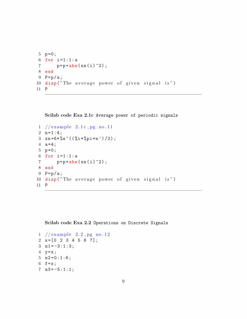
Scilab code Exa 2.2 Operations on Discrete Signals
1 // example 2 . 2 , pg no . 1 22 x=[0 2 3 4 5 6 7];
3 n1= -3:1:3;
4 y=x;
5 n2 =0:1:6;
6 f=x;
7 n3= -5:1:1;
9
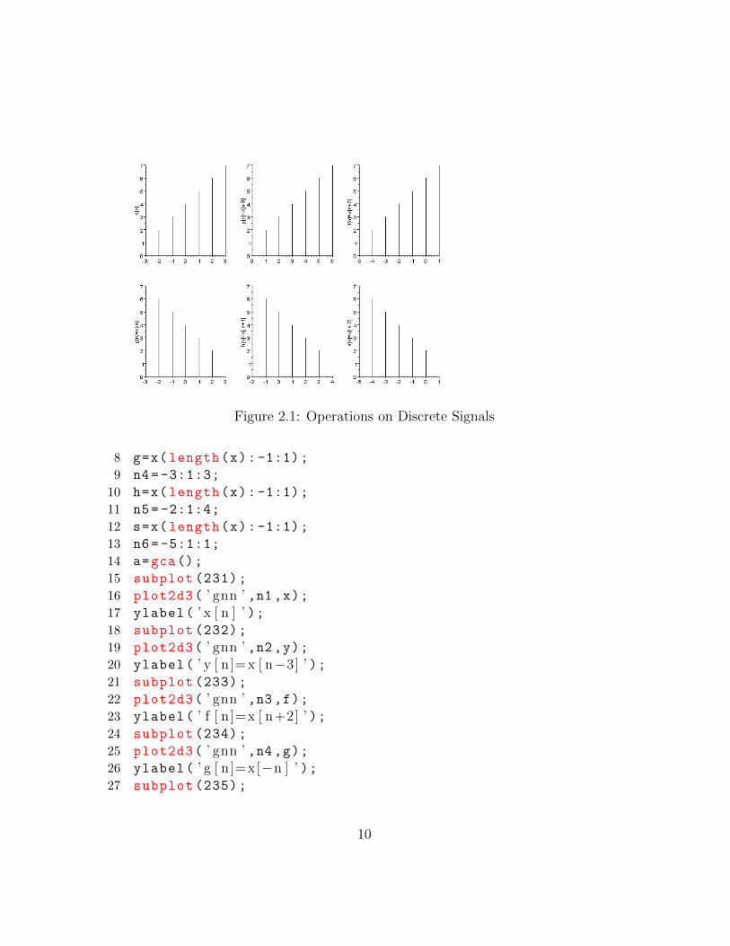
Figure 2.1: Operations on Discrete Signals
8 g=x(length(x): -1:1);
9 n4= -3:1:3;
10 h=x(length(x): -1:1);
11 n5= -2:1:4;
12 s=x(length(x): -1:1);
13 n6= -5:1:1;
14 a=gca();
15 subplot (231);
16 plot2d3( ’ gnn ’ ,n1 ,x);17 ylabel( ’ x [ n ] ’ );18 subplot (232);
19 plot2d3( ’ gnn ’ ,n2 ,y);20 ylabel( ’ y [ n]=x [ n−3] ’ );21 subplot (233);
22 plot2d3( ’ gnn ’ ,n3 ,f);23 ylabel( ’ f [ n ]=x [ n+2] ’ );24 subplot (234);
25 plot2d3( ’ gnn ’ ,n4 ,g);26 ylabel( ’ g [ n]=x[−n ] ’ );27 subplot (235);
10
28 plot2d3( ’ gnn ’ ,n5 ,h);29 ylabel( ’ h [ n]=x[−n+1] ’ );30 subplot (236);
31 plot2d3( ’ gnn ’ ,n6 ,s);32 ylabel( ’ s [ n]=x[−n−2] ’ );
Scilab code Exa 2.3a Even and Odd parts of Discrete signals
1 // example 2 . 3 a pg . no . 1 42 clear;clc;close;
3 n=-2:2;
4 x1=[4 -2 4 -6 0];
5 x2=0.5*x1 //x [ n ]6 x3 =0.5*[ x1(length(x1):-1:1)]; //x[−n ]7 xe=(x2+x3);// even pa r t8 xo=(x2-x3);// odd pa r t9 a=gca();
10 a.thickness =2;
11 a.x_location=” middle ”;12 a.y_location=” middle ”;13 plot2d3( ’ gnn ’ ,n,xe,rect=[-4 -6 4 6])
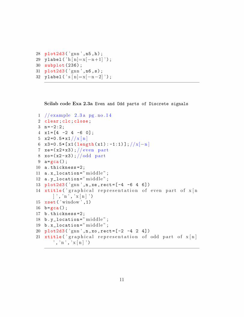
14 xtitle( ’ g r a p h i c a l r e p r e s e n t a t i o n o f even pa r t o f x [ n] ’ , ’ n ’ , ’ x [ n ] ’ )
15 xset( ’ window ’ ,1)16 b=gca();
17 b.thickness =2;
18 b.y_location=” middle ”;19 b.x_location=” middle ”;20 plot2d3( ’ gnn ’ ,n,xo,rect=[-2 -4 2 4])
21 xtitle( ’ g r a p h i c a l r e p r e s e n t a t i o n o f odd pa r t o f x [ n ]’ , ’ n ’ , ’ x [ n ] ’ )
11
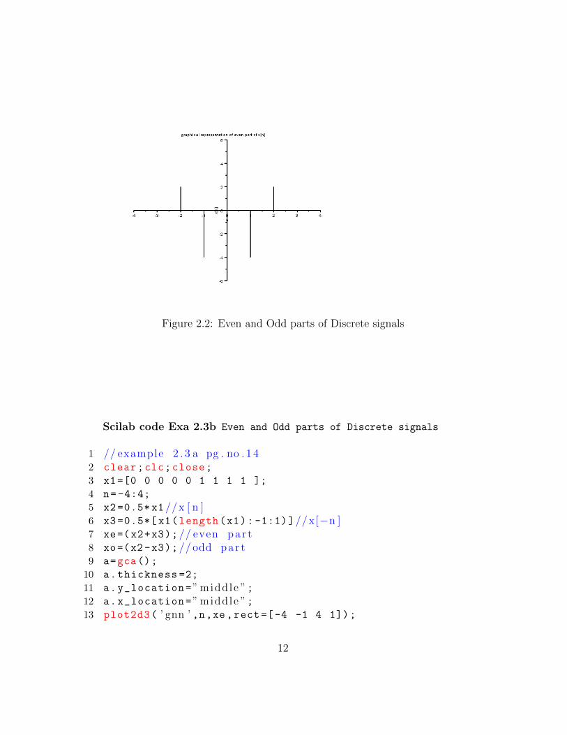
Figure 2.2: Even and Odd parts of Discrete signals
Scilab code Exa 2.3b Even and Odd parts of Discrete signals
1 // example 2 . 3 a pg . no . 1 42 clear;clc;close;
3 x1=[0 0 0 0 0 1 1 1 1 ];
4 n=-4:4;
5 x2=0.5*x1 //x [ n ]6 x3 =0.5*[ x1(length(x1):-1:1)]//x[−n ]7 xe=(x2+x3);// even pa r t8 xo=(x2-x3);// odd pa r t9 a=gca();
10 a.thickness =2;
11 a.y_location=” middle ”;12 a.x_location=” middle ”;13 plot2d3( ’ gnn ’ ,n,xe,rect=[-4 -1 4 1]);
12
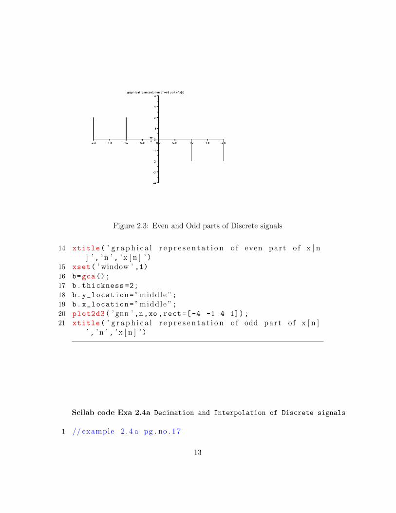
Figure 2.3: Even and Odd parts of Discrete signals
14 xtitle( ’ g r a p h i c a l r e p r e s e n t a t i o n o f even pa r t o f x [ n] ’ , ’ n ’ , ’ x [ n ] ’ )
15 xset( ’ window ’ ,1)16 b=gca();
17 b.thickness =2;
18 b.y_location=” middle ”;19 b.x_location=” middle ”;20 plot2d3( ’ gnn ’ ,n,xo,rect=[-4 -1 4 1]);
21 xtitle( ’ g r a p h i c a l r e p r e s e n t a t i o n o f odd pa r t o f x [ n ]’ , ’ n ’ , ’ x [ n ] ’ )
Scilab code Exa 2.4a Decimation and Interpolation of Discrete signals
1 // example 2 . 4 a pg . no . 1 7
13
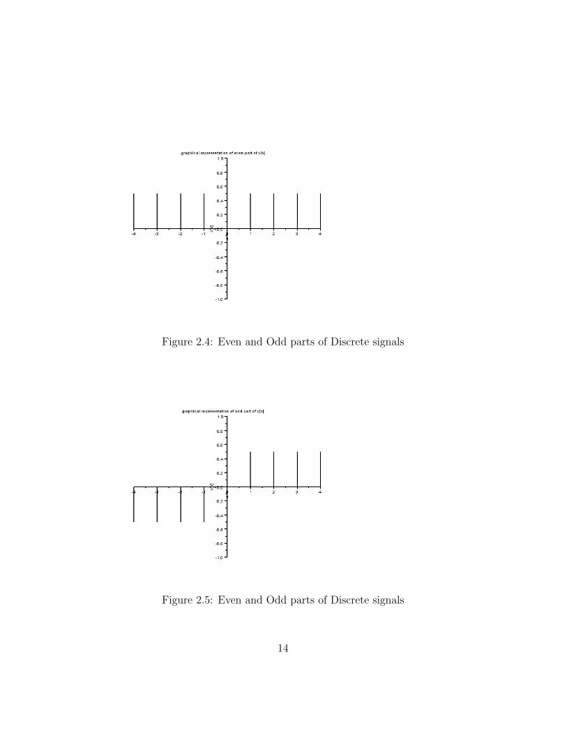
Figure 2.4: Even and Odd parts of Discrete signals
Figure 2.5: Even and Odd parts of Discrete signals
14
2 x=[1 2 5 -1];
3 xm=2; // d e n o t e s 2nd sample has pad .4 y=[x(1:2:xm -2),x(xm:2: length(x))]// dec imat i on5 h=[x(1:1/3: length(x))]// s t e p i n t e r p o l a t e d6 g=h;
7 for i=2:3
8 g(i:3: length(g))=0;
9 end
10 // z e r o i n t e r p o l a t e d11 x1 =1:3:3* length(x);
12 s=interpln ([x1;x] ,1:10) // l i n e a r i n t e r p o l a t e d
Scilab code Exa 2.4b Decimation and Interpolation of Discrete signals
1 // example 2 . 4 b , c . pg . no . 1 72 x=[3 4 5 6];
3 xm=3; // d e n o t e s 3 rd sample has pad4 xm=xm -1; // s h i f t i n g5 g=[x(xm -2: -2:1),x(xm:2: length(x))]// dec imat i on6 xm=3;
7 h=[x(1:1/2: length(x))]// s t e p i n t e r p o l a t e d
Scilab code Exa 2.4c Decimation and Interpolation of Discrete signals
1 // example 2 . 4 c , pg . no . 1 72 x=[3 4 5 6];
3 xm=3;
4 xm=xm+1*(xm -1);// s h i f t i n pad due to i n t e r p o l a t i o n5 xm=xm -2 // normal s h i f t i n g6 x1=[x(1:1/3: length(x))]// s t e p i n t e r p o l a t e d7 xm=3;
8 xm=xm+2*(xm -1) // s h i f t i n pad due to i n t e r p o l a t i o n9 y=[x1(1:2:xm -2),x1(xm:2: length(x1))]// dec imat i on
15
Scilab code Exa 2.4d Decimation and Interpolation of Discrete signals
1 // example 2 . 4 d , pg . no . 1 72 x=[2 4 6 8]
3 xm=3; // denote 3 rd sample has pad4 x1=[1 3 5 7]
5 x2=interpln ([x1;x],1:6)
6 xm=xm+1*(xm -1);// s h i f t i n pad due to i n t e r p o l a t i o n7 xm=xm -1 // s h i f t i n pad due to d e l a y8 y=[x2(2:2:xm -2),x2(xm:2: length(x2))]// dec imat i on
Scilab code Exa 2.5 Describing Sequences and signals
1 // example 2 . 5 , pg . no . 2 02 x=[1 2 4 8 16 32 64];
3 y=[0 0 0 1 0 0 0];
4 z=x.*y;
5 a=0;
6 for i=1: length(z)
7 a=a+z(i);
8 end
9 z,a// a=summation o f z
Scilab code Exa 2.6 Discrete time Harmonics and Periodicity
1 // example 2 . 6 pg . no . 2 32 function[p]= period(x)
3 for i=2: length(x)
4 v=i
16
5 if (abs(x(i)-x(1)) <0.00001)
6 k=2
7 for j=i+1:i+i
8 if (abs(x(j)-x(k)) <0.00001)
9 v=v+1
10 end
11 k=k+1;
12 end
13 end
14 if (v==(2*i)) then
15 break
16 end
17 end
18 p=i-1
19 endfunction
20 for i=1:60
21 x1(i)=cos ((2* %pi*8*i)/25);
22 end
23 for i=1:60
24 x2(i)=exp(%i*0.2*i*%pi)+exp(-%i*0.3*i*%pi);
25 end
26 for i=1:45
27 x3(i)=2* cos ((40* %pi*i)/75)+sin ((60* %pi*i)/75);
28 end
29 period(x1)
30 period(x2)
31 period(x3)
check Appendix AP 1 for dependency:
Aliasfrequency.sci
Scilab code Exa 2.7 Aliasing and its effects
1 // example 2 . 7 . pg . no . 2 72 f=100;
17
3 s=240;
4 s1=s;
5 aliasfrequency(f,s)
6 s=140;
7 s1=s;
8 aliasfrequency(f,s,s1)
9 s=90;
10 s1=s;
11 aliasfrequency(f,s,s1)
12 s=35;
13 s1=s;
14 aliasfrequency(f,s,s1)
check Appendix AP 1 for dependency:
Aliasfrequency.sci
Scilab code Exa 2.8 Signal Reconstruction
1 f=100;
2 s=210;
3 s1=420;
4 aliasfrequency(f,s,s1)
5 s=140;
6 aliasfrequency(f,s,s1)
18
Chapter 3
Response of Digital Filters
Scilab code Exa 3.5 FIR filter response
1 // Response o f non−r e c u r s i v e F i l t e r s2 for i=1:4
3 x(i)=0.5^i;
4 end
5 x1 =[0;1;x(1:2)]
6 for i=1:4
7 y(i)=2*x(i) -3*x1(i);
8 end
9 y(1),y(2)
Scilab code Exa 3.19a Analytical Evaluation of Discrete Convolution
1 // A n a l y t i c a l e v a l u a t i o n o f D i s c r e t e Convo lu t i on2 clear;close;clc;
3 max_limit =10;
4 h=ones(1,max_limit);
5 n2=0: length(h) -1;
6 x=h;
19
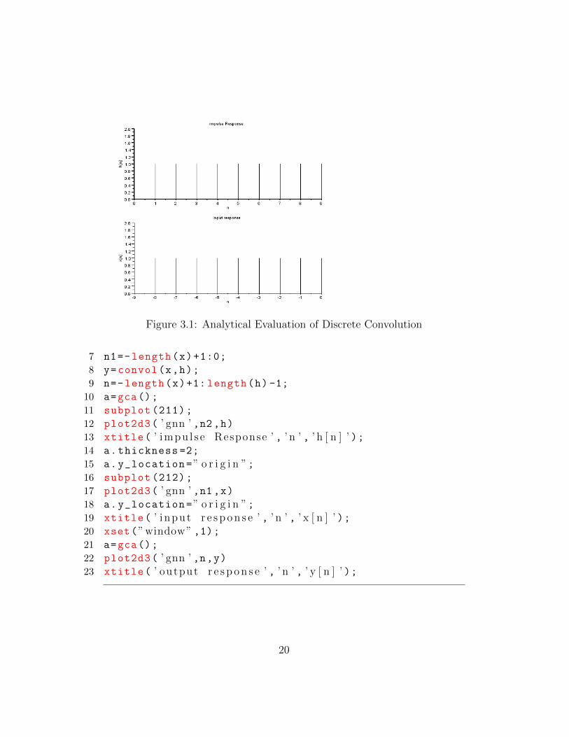
Figure 3.1: Analytical Evaluation of Discrete Convolution
7 n1=-length(x)+1:0;
8 y=convol(x,h);
9 n=-length(x)+1: length(h) -1;
10 a=gca();
11 subplot (211);
12 plot2d3( ’ gnn ’ ,n2 ,h)13 xtitle( ’ impu l s e Response ’ , ’ n ’ , ’ h [ n ] ’ );14 a.thickness =2;
15 a.y_location=” o r i g i n ”;16 subplot (212);
17 plot2d3( ’ gnn ’ ,n1 ,x)18 a.y_location=” o r i g i n ”;19 xtitle( ’ i npu t r e s p o n s e ’ , ’ n ’ , ’ x [ n ] ’ );20 xset(”window” ,1);21 a=gca();
22 plot2d3( ’ gnn ’ ,n,y)23 xtitle( ’ output r e s p o n s e ’ , ’ n ’ , ’ y [ n ] ’ );
20
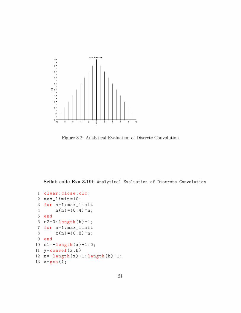
Figure 3.2: Analytical Evaluation of Discrete Convolution
Scilab code Exa 3.19b Analytical Evaluation of Discrete Convolution
1 clear;close;clc;
2 max_limit =10;
3 for n=1: max_limit
4 h(n)=(0.4)^n;
5 end
6 n2=0: length(h) -1;
7 for n=1: max_limit
8 x(n)=(0.8)^n;
9 end
10 n1=-length(x)+1:0;
11 y=convol(x,h)
12 n=-length(x)+1: length(h) -1;
13 a=gca();
21
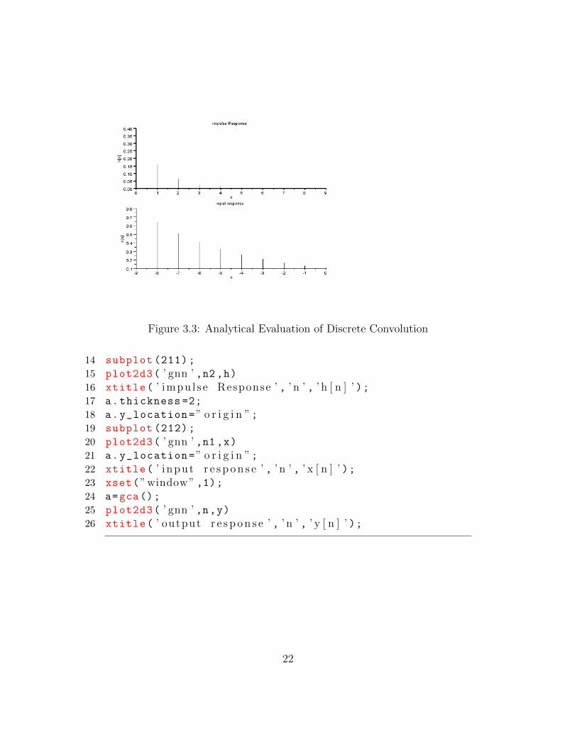
Figure 3.3: Analytical Evaluation of Discrete Convolution
14 subplot (211);
15 plot2d3( ’ gnn ’ ,n2 ,h)16 xtitle( ’ impu l s e Response ’ , ’ n ’ , ’ h [ n ] ’ );17 a.thickness =2;
18 a.y_location=” o r i g i n ”;19 subplot (212);
20 plot2d3( ’ gnn ’ ,n1 ,x)21 a.y_location=” o r i g i n ”;22 xtitle( ’ i npu t r e s p o n s e ’ , ’ n ’ , ’ x [ n ] ’ );23 xset(”window” ,1);24 a=gca();
25 plot2d3( ’ gnn ’ ,n,y)26 xtitle( ’ output r e s p o n s e ’ , ’ n ’ , ’ y [ n ] ’ );
22
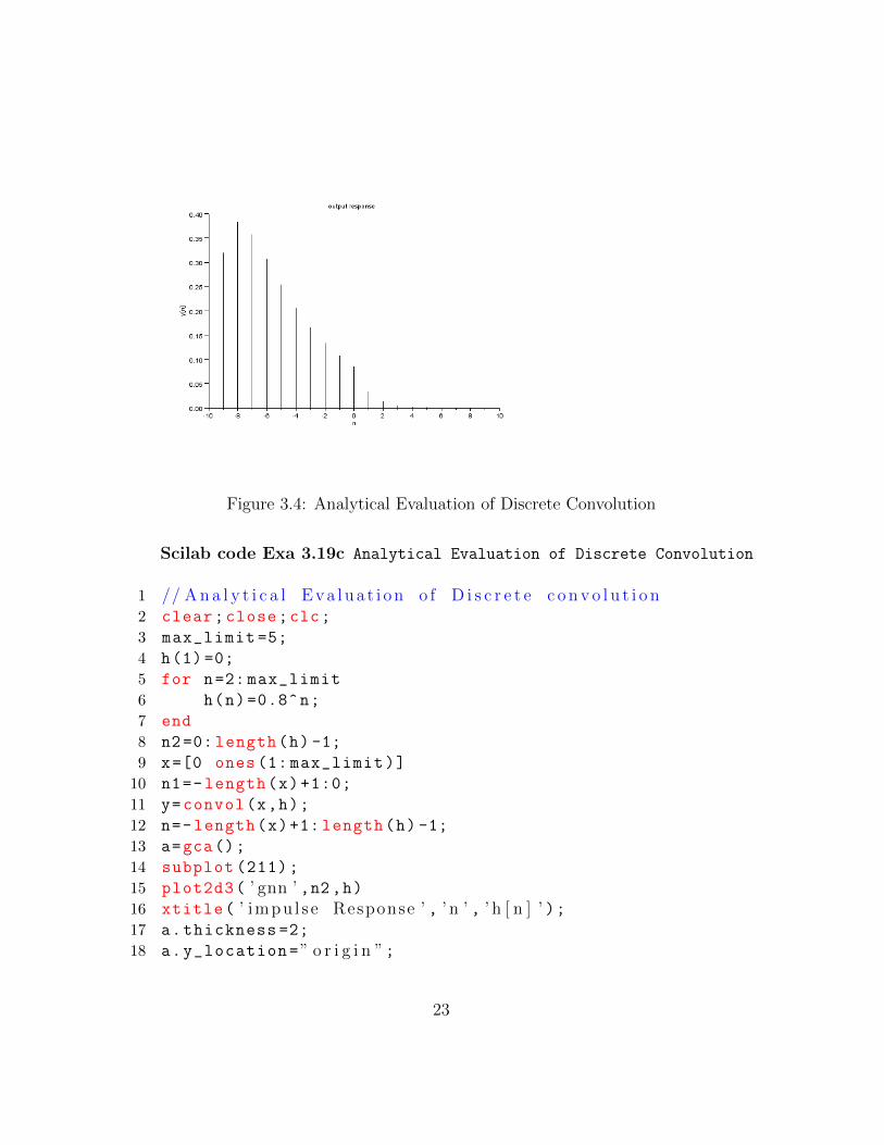
Figure 3.4: Analytical Evaluation of Discrete Convolution
Scilab code Exa 3.19c Analytical Evaluation of Discrete Convolution
1 // A n a l y t i c a l E v a l u a t i o n o f D i s c r e t e c o n v o l u t i o n2 clear;close;clc;
3 max_limit =5;
4 h(1)=0;
5 for n=2: max_limit
6 h(n)=0.8^n;
7 end
8 n2=0: length(h) -1;
9 x=[0 ones (1: max_limit)]
10 n1=-length(x)+1:0;
11 y=convol(x,h);
12 n=-length(x)+1: length(h) -1;
13 a=gca();
14 subplot (211);
15 plot2d3( ’ gnn ’ ,n2 ,h)16 xtitle( ’ impu l s e Response ’ , ’ n ’ , ’ h [ n ] ’ );17 a.thickness =2;
18 a.y_location=” o r i g i n ”;
23
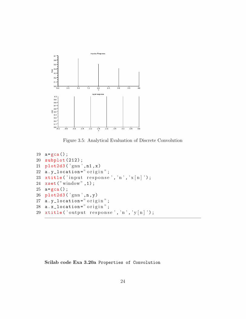
Figure 3.5: Analytical Evaluation of Discrete Convolution
19 a=gca();
20 subplot (212);
21 plot2d3( ’ gnn ’ ,n1 ,x)22 a.y_location=” o r i g i n ”;23 xtitle( ’ i npu t r e s p o n s e ’ , ’ n ’ , ’ x [ n ] ’ );24 xset(”window” ,1);25 a=gca();
26 plot2d3( ’ gnn ’ ,n,y)27 a.y_location=” o r i g i n ”;28 a.x_location=” o r i g i n ”;29 xtitle( ’ output r e s p o n s e ’ , ’ n ’ , ’ y [ n ] ’ );
Scilab code Exa 3.20a Properties of Convolution
24
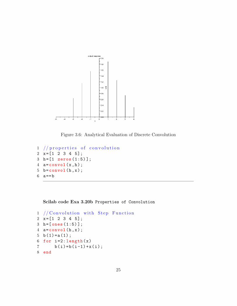
Figure 3.6: Analytical Evaluation of Discrete Convolution
1 // p r o p e r t i e s o f c o n v o l u t i o n2 x=[1 2 3 4 5];
3 h=[1 zeros (1:5)];
4 a=convol(x,h);
5 b=convol(h,x);
6 a==b
Scilab code Exa 3.20b Properties of Convolution
1 // Convo lu t i on with Step Funct ion2 x=[1 2 3 4 5];
3 h=[ones (1:5)];
4 a=convol(h,x);
5 b(1)=a(1);
6 for i=2: length(x)
7 b(i)=b(i-1)+x(i);
8 end
25
9 disp(a(1: length(x)),b, ’ Step Response i s runn ing sumo f i m p u l s e s can be s e en below ’ );
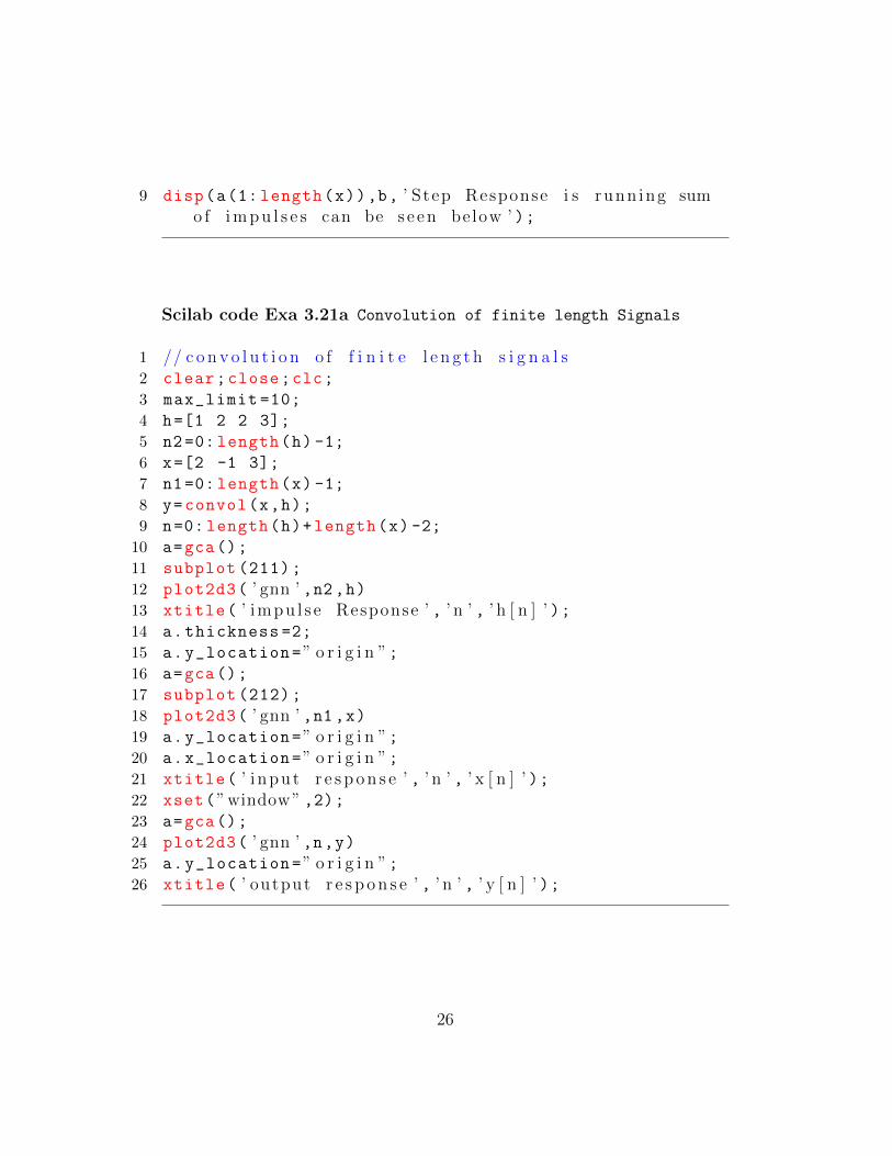
Scilab code Exa 3.21a Convolution of finite length Signals
1 // c o n v o l u t i o n o f f i n i t e l e n g t h s i g n a l s2 clear;close;clc;
3 max_limit =10;
4 h=[1 2 2 3];
5 n2=0: length(h) -1;
6 x=[2 -1 3];
7 n1=0: length(x) -1;
8 y=convol(x,h);
9 n=0: length(h)+length(x) -2;
10 a=gca();
11 subplot (211);
12 plot2d3( ’ gnn ’ ,n2 ,h)13 xtitle( ’ impu l s e Response ’ , ’ n ’ , ’ h [ n ] ’ );14 a.thickness =2;
15 a.y_location=” o r i g i n ”;16 a=gca();
17 subplot (212);
18 plot2d3( ’ gnn ’ ,n1 ,x)19 a.y_location=” o r i g i n ”;20 a.x_location=” o r i g i n ”;21 xtitle( ’ i npu t r e s p o n s e ’ , ’ n ’ , ’ x [ n ] ’ );22 xset(”window” ,2);23 a=gca();
24 plot2d3( ’ gnn ’ ,n,y)25 a.y_location=” o r i g i n ”;26 xtitle( ’ output r e s p o n s e ’ , ’ n ’ , ’ y [ n ] ’ );
26
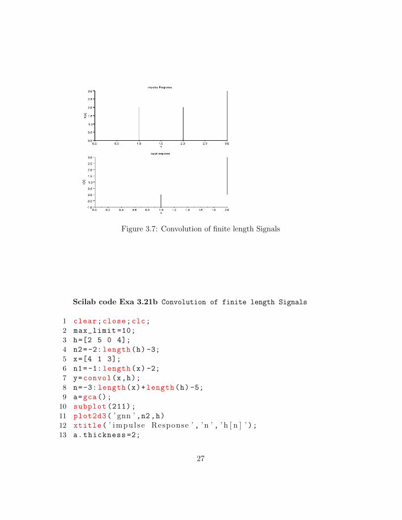
Figure 3.7: Convolution of finite length Signals
Scilab code Exa 3.21b Convolution of finite length Signals
1 clear;close;clc;
2 max_limit =10;
3 h=[2 5 0 4];
4 n2=-2: length(h) -3;
5 x=[4 1 3];
6 n1=-1: length(x) -2;
7 y=convol(x,h);
8 n=-3: length(x)+length(h) -5;
9 a=gca();
10 subplot (211);
11 plot2d3( ’ gnn ’ ,n2 ,h)12 xtitle( ’ impu l s e Response ’ , ’ n ’ , ’ h [ n ] ’ );13 a.thickness =2;
27
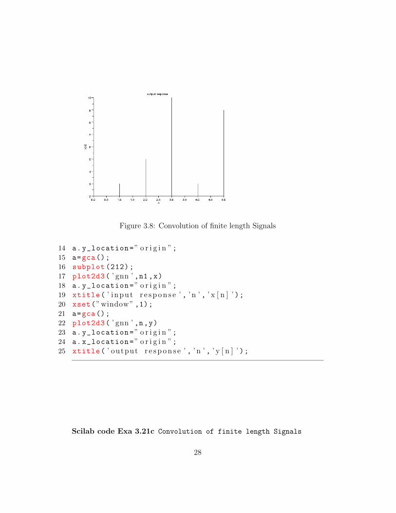
Figure 3.8: Convolution of finite length Signals
14 a.y_location=” o r i g i n ”;15 a=gca();
16 subplot (212);
17 plot2d3( ’ gnn ’ ,n1 ,x)18 a.y_location=” o r i g i n ”;19 xtitle( ’ i npu t r e s p o n s e ’ , ’ n ’ , ’ x [ n ] ’ );20 xset(”window” ,1);21 a=gca();
22 plot2d3( ’ gnn ’ ,n,y)23 a.y_location=” o r i g i n ”;24 a.x_location=” o r i g i n ”;25 xtitle( ’ output r e s p o n s e ’ , ’ n ’ , ’ y [ n ] ’ );
Scilab code Exa 3.21c Convolution of finite length Signals
28
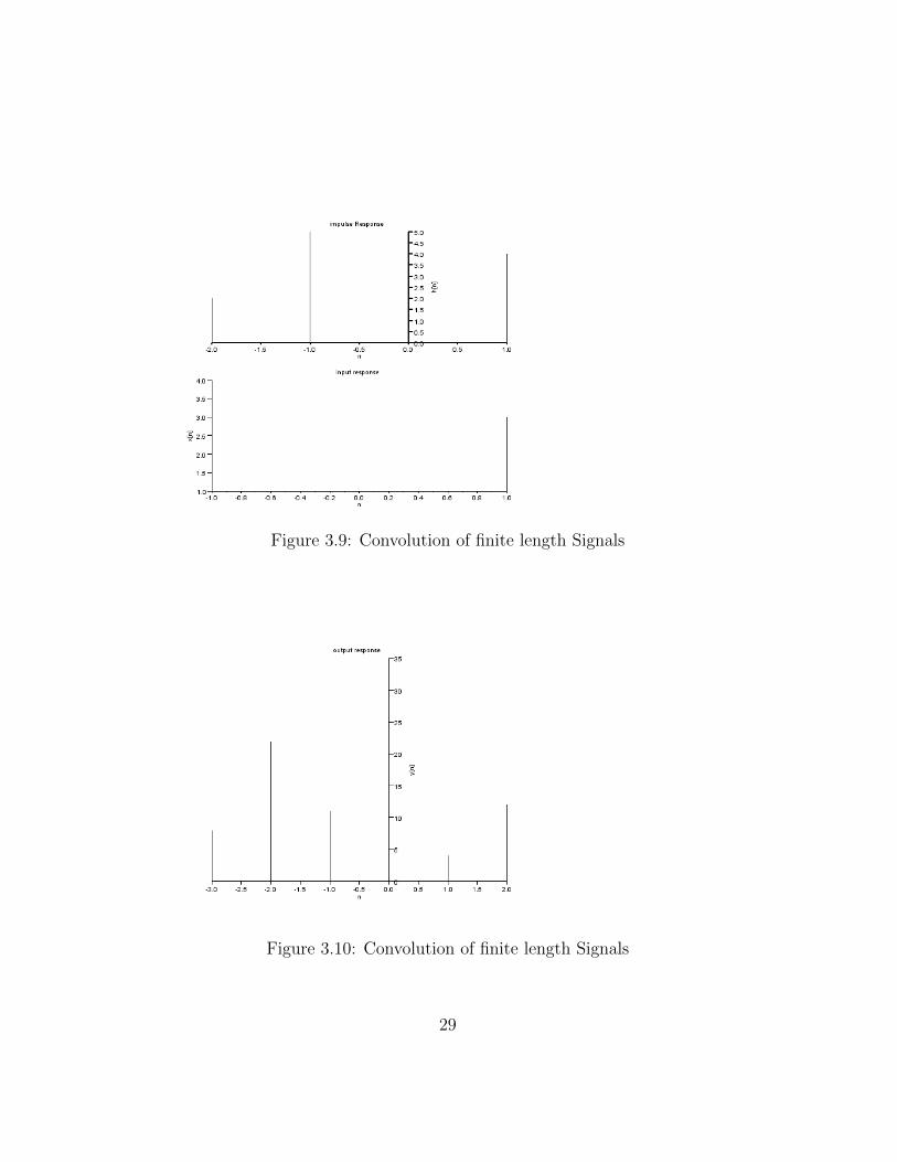
Figure 3.9: Convolution of finite length Signals
Figure 3.10: Convolution of finite length Signals
29
1 clear;close;clc;
2 max_limit =10;
3 h=[1/2 1/2 1/2];
4 n2=0: length(h) -1;
5 x=[2 4 6 8 10];
6 n1=0: length(x) -1;
7 y=convol(x,h);
8 n=0: length(x)+length(h) -2;
9 a=gca();
10 subplot (211);
11 plot2d3( ’ gnn ’ ,n2 ,h);12 xtitle( ’ impu l s e Response ’ , ’ n ’ , ’ h [ n ] ’ );13 a.thickness =2;
14 a.y_location=” o r i g i n ”;15 a=gca();
16 subplot (212);
17 plot2d3( ’ gnn ’ ,n1 ,x);18 a.y_location=” o r i g i n ”;19 xtitle( ’ i npu t r e s p o n s e ’ , ’ n ’ , ’ x [ n ] ’ );20 xset(”window” ,1);21 a=gca();
22 plot2d3( ’ gnn ’ ,n,y)23 a.y_location=” o r i g i n ”;24 a.x_location=” o r i g i n ”;25 xtitle( ’ output r e s p o n s e ’ , ’ n ’ , ’ y [ n ] ’ );
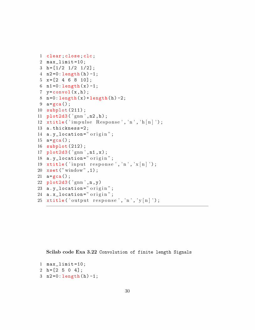
Scilab code Exa 3.22 Convolution of finite length Signals
1 max_limit =10;
2 h=[2 5 0 4];
3 n2=0: length(h) -1;
30
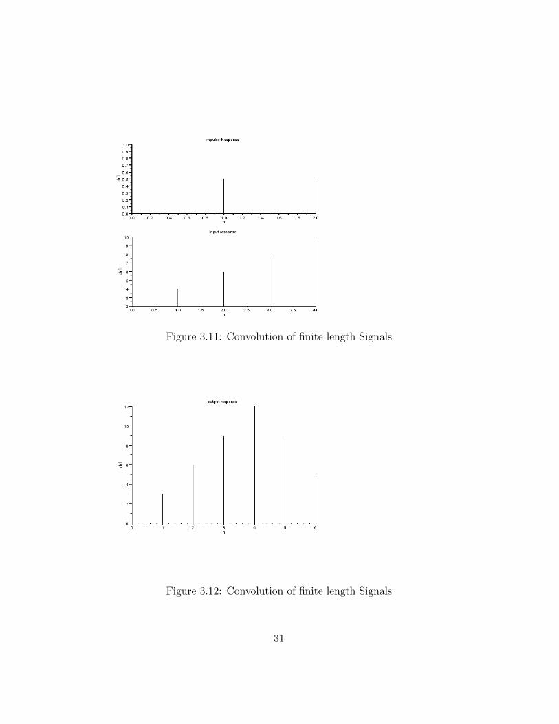
Figure 3.11: Convolution of finite length Signals
Figure 3.12: Convolution of finite length Signals
31

4 x=[4 1 3];
5 n1=0: length(x) -1;
6 y=convol(x,h);
7 n=0: length(x)+length(h) -2;
8 a=gca();
9 subplot (211);
10 plot2d3( ’ gnn ’ ,n2 ,h)11 xtitle( ’ impu l s e Response ’ , ’ n ’ , ’ h [ n ] ’ );12 a.thickness =2;
13 a.y_location=” o r i g i n ”;14 a=gca();
15 subplot (212);
16 plot2d3( ’ gnn ’ ,n1 ,x)17 a.y_location=” o r i g i n ”;18 a.x_location=” o r i g i n ”;19 xtitle( ’ i npu t r e s p o n s e ’ , ’ n ’ , ’ x [ n ] ’ );20 xset(”window” ,1);21 a=gca();
22 plot2d3( ’ gnn ’ ,n,y)23 a.y_location=” o r i g i n ”;24 a.x_location=” o r i g i n ”;25 xtitle( ’ output r e s p o n s e ’ , ’ n ’ , ’ y [ n ] ’ );
Scilab code Exa 3.23 effect of Zero Insertion,Zero Padding on convol.
1 // c o n v o l u t i o n by po lynomia l method2 x=[4 1 3];
3 h=[2 5 0 4];
4 z=%z;
5 n=length(x) -1:-1:0;
6 X=x*z^n’;
32
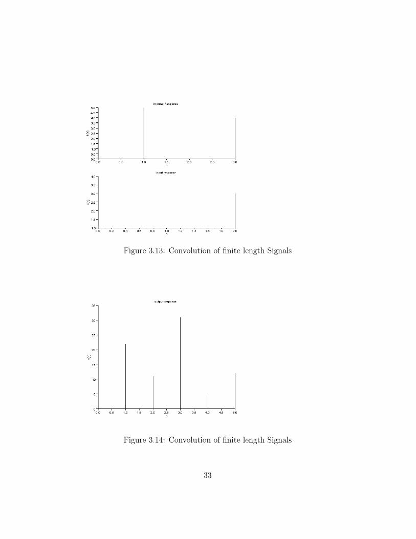
Figure 3.13: Convolution of finite length Signals
Figure 3.14: Convolution of finite length Signals
33
7 n1=length(h) -1:-1:0;
8 H=h*z^n1 ’;
9 y=X*H
10 // e f f e c t o f z e r o i n s e r t i o n on c o n v o l u t i o n11 h=[2 0 5 0 0 0 4];
12 x=[4 0 1 0 3];
13 y=convol(x,h)
14 // e f f e c t o f z e r o padding on c o n v o l u t i o n15 h=[2 5 0 4 0 0];
16 x=[4 1 3 0];
17 y=convol(x,h)
Scilab code Exa 3.25 Stability and Causality
1 // c o n c e p t s based on s t a b i l i t y and C a u s a l i t y2 function []= stability(X)
3 if (abs(roots(X)) <1)
4 disp(” g i v e n system i s s t a b l e ”)5 else
6 disp(” g i v e n system i s not s t a b l e ”)7 end
8 endfunction
9 x=[1 -1/6 -1/6];
10 z=%z;
11 n=length(x) -1:-1:0;
12 // c h a r a c t e r i s t i c eqn i s13 X=x*(z)^n’
14 stability(X)
15 x=[1 -1];
16 n=length(x) -1:-1:0;
17 // c h a r a c t e r i s t i c eqn i s18 X=x*(z)^n’
19 stability(X)
20 x=[1 -2 1];
21 n=length(x) -1:-1:0;
34
22 // c h a r a c t e r i s t i c eqn i s23 X=x*(z)^n’
24 stability(X)
Scilab code Exa 3.26 Response to Periodic Inputs
1 // Response o f p e r i o d i c i n p u t s2 function[p]= period(x)
3 for i=2: length(x)
4 v=i
5 if (abs(x(i)-x(1)) <0.00001)
6 k=2
7 for j=i+1:i+i
8 if (abs(x(j)-x(k)) <0.00001)
9 v=v+1
10 end
11 k=k+1;
12 end
13 end
14 if (v==(2*i)) then
15 break
16 end
17 end
18 p=i-1
19 endfunction
20 x=[1 2 -3 1 2 -3 1 2 -3];
21 h=[1 1];
22 y=convol(x,h)
23 y(1)=y(4);
24 period(x)
25 period(y)
26 h=[1 1 1];
27 y=convol(x,h)
35
Scilab code Exa 3.27 Periodic Extension
1 // to f i n d p e r i o d i c e x t e n s i o n2 x=[1 5 2;0 4 3;6 7 0];
3 y=[0 0 0];
4 for i=1:3
5 for j=1:3
6 y(i)=y(i)+x(j,i);
7 end
8 end
9 y
Scilab code Exa 3.28 System Response to Periodic Inputs
1 // method o f wrapping to f i n g c o n v o l u t i o n o f p e r i o d i cs i g n a l with one p e r i o d
2 x=[1 2 -3];
3 h=[1 1];
4 y1=convol(h,x)
5 y1=[y1,zeros (5:9)]
6 y2=[y1 (1:3);y1 (4:6);y1(7:9)];
7 y=[0 0 0];
8 for i=1:3
9 for j=1:3
10 y(i)=y(i)+y2(j,i);
11 end
12 end
13 y
14 x=[2 1 3];
15 h=[2 1 1 3 1];
16 y1=convol(h,x)
17 y1=[y1,zeros (8:9)]
36
18 y2=[y1 (1:3);y1 (4:6);y1(7:9)];
19 y=[0 0 0];
20 for i=1:3
21 for j=1:3
22 y(i)=y(i)+y2(j,i);
23 end
24 end
25 y
Scilab code Exa 3.29 Periodic Convolution
1 // p e r i o d i c or c i r c u l a r c o n v o l u t i o n2 x=[1 0 1 1];
3 h=[1 2 3 1];
4 y1=convol(h,x)
5 y1=[y1,zeros (8:12) ];
6 y2=[y1 (1:4);y1 (5:8);y1 (9:12) ];
7 y=[0 0 0 0];
8 for i=1:4
9 for j=1:3
10 y(i)=y(i)+y2(j,i);
11 end
12 end
13 y
Scilab code Exa 3.30 Periodic Convolution by Circulant Matrix
1 // p e r i o d i c c o n v o l u t i o n by c i r c u l a n t matr ix2 x=[1 0 2];
3 h=[1;2;3];
4 // g e n e r a t i o n o f c i r c u l a n t matr ix5 c(1,:)=x;
6 for i=2: length(x)
37
7 c(i,:)=[x(length(x):length(x)-i),x(1: length(x)-i
)]
8 end
9 c’
Scilab code Exa 3.32 Deconvolution By polynomial Division
1 // d e c o n v o l u t i o n by po lynomia l d i v i s i o n2 x=[2 5 0 4];
3 y=[8 22 11 31 4 12];
4 z=%z
5 n=length(x) -1:-1:0;
6 X=x*(z)^n’
7 n1=length(y) -1:-1:0;
8 Y=y*(z)^n1’
9 h=Y/X
Scilab code Exa 3.33 Autocorrelation and Cross Correlation
1 // d i s c r e t e auto c o r r e l a t i o n and c r o s s c o r r e l a t i o n2 x=[2 5 0 4];
3 h=[3 1 4];
4 x1=x(length(x): -1:1)
5 h1=h(length(h): -1:1)
6 rxhn=convol(x,h1)
7 rhxn=convol(x1 ,h)
8 rhxn1=rhxn(length(rhxn): -1:1)
9 //we o b s e r v e tha t rhxn1=rxhn10 x=[3 1 -4];
11 x1=x(length(x): -1:1)
12 rxxn=convol(x,x1)
13 //we o b s e r v e tha t rxxn i s even symmetr ic abouto r i g i n
38
Scilab code Exa 3.35 Periodic Autocorrelation and Cross Correlation
1 // d i s c r e t e p e r i o d i c auto c o r r e l a t i o n and c r o s sc o r r e l a t i o n
2 x=[2 5 0 4];
3 h=[3 1 -1 2];
4 x1=x(length(x): -1:1);
5 h1=h(length(h): -1:1);
6 rxhn=convol(x,h1)
7 rhxn=convol(x1 ,h)
8 rxxn=convol(x,x1)
9 rhhn=convol(h,h1)
10 y1=[rxhn ,zeros (8:12) ];
11 y2=[y1 (1:4);y1 (5:8);y1 (9:12) ];
12 y3=[rhxn ,zeros (8:12) ];
13 y4=[y3 (1:4);y3 (5:8);y3 (9:12) ];
14 y5=[rxxn ,zeros (8:12) ];
15 y6=[y5 (1:4);y5 (5:8);y5 (9:12) ];
16 y7=[rhhn ,zeros (8:12) ];
17 y8=[y7 (1:4);y7 (5:8);y7 (9:12) ];
18 rxhp =[0 0 0 0];
19 rhxp =[0 0 0 0];
20 rxxn =[0 0 0 0];
21 rhhp =[0 0 0 0];
22 for i=1:4
23 for j=1:3
24 rhxp(i)=rhxp(i)+y4(j,i);
25 rxhp(i)=rxhp(i)+y2(j,i);
26 rxxn(i)=rxxn(i)+y6(j,i);
27 rhhp(i)=rhhp(i)+y8(j,i);
28 end
29 end
30 rxhp
31 rhxp
39

32 rxxn
33 rhhp
40
Chapter 4
z Transform Analysis
Scilab code Exa 4.1b z transform of finite length sequences
1 function[za]= ztransfer(sequence ,n)
2 z=poly(0, ’ z ’ , ’ r ’ )3 za=sequence *(1/z)^n’
4 endfunction
5 x1=[2 1 -5 4];
6 n=-1: length(x1) -2;
7 ztransfer(x1 ,n)
Scilab code Exa 4.4a Pole Zero Plots
1 // Pole−Zero p l o t s2 z=%z;
3 az=2*z*(z+1);
4 bz=(z -1/3) *((z^2) +1/4) *((z^2) +4*z+5);
5 poles=roots(bz)
6 zeroes=roots(az)
7 h=az/bz
41
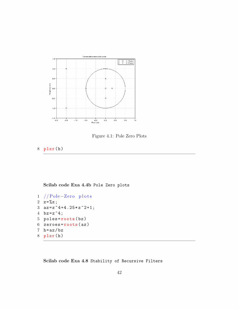
Figure 4.1: Pole Zero Plots
8 plzr(h)
Scilab code Exa 4.4b Pole Zero plots
1 // Pole−Zero p l o t s2 z=%z;
3 az=z^4+4.25*z^2+1;
4 bz=z^4;
5 poles=roots(bz)
6 zeroes=roots(az)
7 h=az/bz
8 plzr(h)
Scilab code Exa 4.8 Stability of Recursive Filters
42
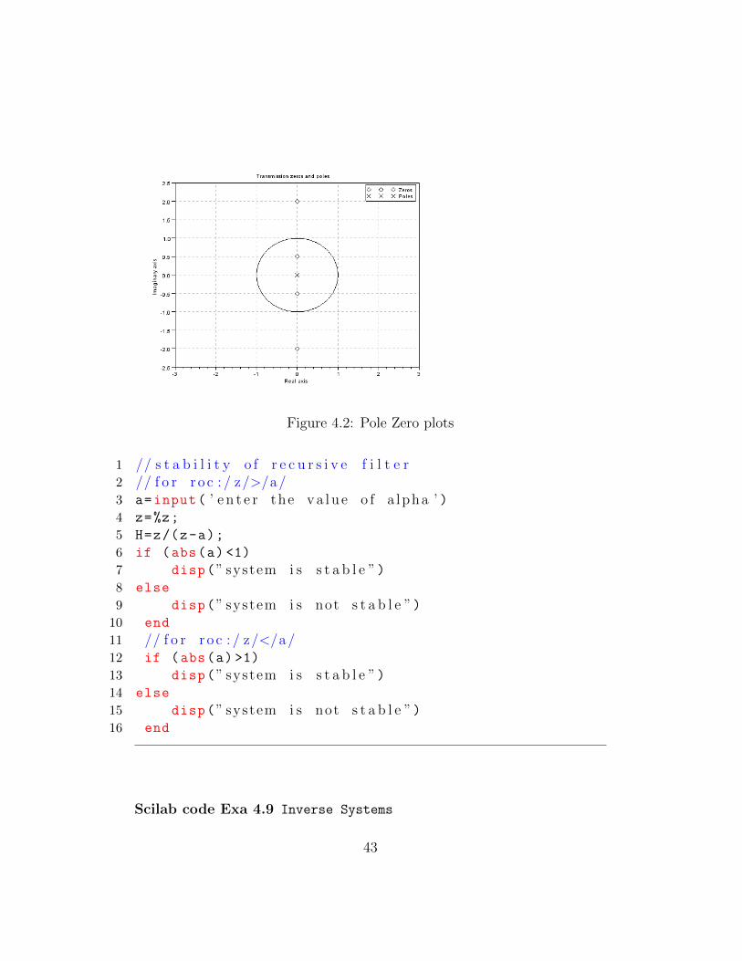
Figure 4.2: Pole Zero plots
1 // s t a b i l i t y o f r e c u r s i v e f i l t e r2 // f o r r o c : / z/>/a/3 a=input( ’ e n t e r the v a l u e o f a lpha ’ )4 z=%z;
5 H=z/(z-a);
6 if (abs(a) <1)
7 disp(” system i s s t a b l e ”)8 else
9 disp(” system i s not s t a b l e ”)10 end
11 // f o r r o c : / z/</a/12 if (abs(a) >1)
13 disp(” system i s s t a b l e ”)14 else
15 disp(” system i s not s t a b l e ”)16 end
Scilab code Exa 4.9 Inverse Systems
43
1 // i n v e r s e sy s t ems2 z=%z;
3 H=(1+2*(z^(-1)))/(1+3*(z^(-1)));
4 // i n v e r s e o f H i s5 H1=1/H
6 H=1+2*(z^(-1))+3*(z^(-2));
7 H1=1/H
Scilab code Exa 4.10 Inverse Transform of sequences
1 // i n v e r s e t r a n s f o r m o f s e q u e n c e s2 // ( a )X( z )=3zˆ−1+5zˆ−3+2zˆ−43 z=%z;
4 X1=[3*z^ -1;0;5*z^-3;2*z^-4];
5 n1=1:4;
6 ZI=z^n1 ’;
7 x1=numer(X1.*ZI);
8 disp(x1,”x [ n]=”);9 // ( b )X( z )=2zˆ2−5z+5zˆ−1−2zˆ−2
10 X2=[2*z^2; -5*z;0;5*z^-1;-2*z^-2];
11 n2= -2:2;
12 ZI=z^n2 ’;
13 x2=numer(X2.*ZI);
14 disp(x2,”x [ n]=”);
Scilab code Exa 4.11 Inverse Transform by Long Division
1 // i n v e r s e t r a n s f o r m by l ong d i v i s i o n2 z=%z;
3 x=ldiv(z-4,1-z+z^2,5)
44
Scilab code Exa 4.12 Inverse transform of Right sided sequences
1 // i n v e r s e z t r a n s f o r m s from standard t r a n s f o r m s2 z=%z;
3 xz=z/((z-0.5) *(z -0.25));
4 yz=xz/z;
5 pfss(yz)
6 // hence x [ n ]= −4(0 .25) ˆn∗un +4(0 . 5 ) ˆn∗un ;7 xz=1/((z-0.5) *(z -0.25));
8 yz=xz/z;
9 pfss(yz)
10 // hence x [ n ]= −4(0 .25) ˆn−1∗u [ n−1 ]+4(0 .5 ) ˆn−1∗u [ n−1 ] ;
Scilab code Exa 4.20 z Transform of Switched periodic Signals
1 // z t r a n s f o r m o f s w i t c h e d p e r i o d i c s i g n a l s2 z=%z;
3 // s o l . f o r 4 . 2 0 a4 x1=[0 1 2];
5 n=0:2;
6 N=3;
7 x1z=x1*(1/z)^n’
8 xz=x1z/(1-z^-N)
9 // s o l . f o r 4 . 2 0 b10 x1=[0 1 0 -1];
11 n=0:3;
12 N=4;
13 x1z=x1*(1/z)^n’
14 xz=x1z/(1-z^-N)
15 // s o l . f o r 4 . 2 0 c16 xz=(2+z^-1)/(1-z^-3);
17 x1z=numer(xz)
18 // thus f i r s t p e r i o d o f xn i s [ 2 1 0 ]19 // s o l . f o r 4 . 2 0 d20 xz=(z^-1-z^-4)/(1-z^-6);
45
21 x1z=numer(xz)
22 // thus f i r s t p e r i o d o f xn i s [ 0 1 0 0 −1 0 ]
46
Chapter 5
Frequency Domain Analysis
Scilab code Exa 5.1c DTFT from Defining Relation
1 //DTFT o f x [ n ]=( a ) ˆn∗u [ n ]2 clear;
3 clc;close;
4 //DTS s i g n a l5 a1=0.5;
6 a2= -0.5;
7 max_limit =10;
8 for n=0: max_limit -1
9 x1(n+1)=(a1^n);
10 x2(n+1)=(a2^n);
11 end
12 n=0: max_limit -1;
13 // d i s c r e t e t ime f o u r i e r t r a n s f o r m14 wmax =2*%pi;
15 K=4;
16 k=0:(K/1000):K;
17 W=k*wmax/K;
18 x1=x1’
19 x2=x2’
20 XW1=x1*exp(%i*n’*W);
21 XW2=x2*exp(%i*n’*W);
47
22 XW1_Mag=abs(XW1);
23 XW2_Mag=abs(XW2);
24 W=[- mtlb_fliplr(W),W(2:1001) ]; // omega form25 XW1_Mag =[ mtlb_fliplr(XW1_Mag),XW1_Mag (2:1001) ];
26 XW2_Mag =[ mtlb_fliplr(XW2_Mag),XW2_Mag (2:1001) ];
27 [XW1_phase ,db]= phasemag(XW1);
28 [XW2_phase ,db]= phasemag(XW2);
29 XW1_phase=[- mtlb_fliplr(XW1_phase),XW1_phase (2:1001)
];
30 XW2_phase=[- mtlb_fliplr(XW2_phase),XW2_phase (2:1001)
];
31
32 // p l o t f o r a>033 figure
34 subplot (3,1,1);
35 plot2d3( ’ gnn ’ ,n,x1)36 xtitle( ’ D i s c r e t e t ime sequencex [ n ] a>0 ’ )37 subplot (3,1,2);
38 a=gca();
39 a.y_location=” o r i g i n ”;40 a.x_location=” o r i g i n ”;41 plot2d3(W,XW1_Mag);
42 title( ’ magnitude Response abs ( exp ( jw ) ) ’ )43 subplot (3,1,3);
44 a=gca();
45 a.y_location=” o r i g i n ”;46 a.x_location=” o r i g i n ”;47 plot2d(W,XW1_phase);
48 title( ’ magnitude Response abs ( exp ( jw ) ) ’ )49 // p l o t f o r a<050 figure
51 subplot (3,1,1);
52 plot2d3( ’ gnn ’ ,n,x2);53 xtitle( ’ D i s c r e t e Time s equence x [ n ] f o r a>0 ’ )54 subplot (3,1,2);
55 a=gca();
56 a.y_location=” o r i g i n ”;57 a.x_location=” o r i g i n ”;
48
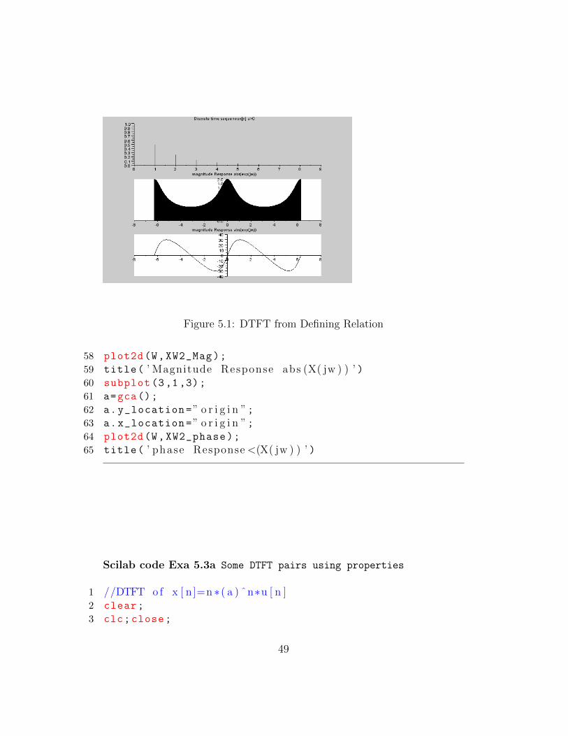
Figure 5.1: DTFT from Defining Relation
58 plot2d(W,XW2_Mag);
59 title( ’ Magnitude Response abs (X( jw ) ) ’ )60 subplot (3,1,3);
61 a=gca();
62 a.y_location=” o r i g i n ”;63 a.x_location=” o r i g i n ”;64 plot2d(W,XW2_phase);
65 title( ’ phase Response <(X( jw ) ) ’ )
Scilab code Exa 5.3a Some DTFT pairs using properties
1 //DTFT o f x [ n]=n ∗ ( a ) ˆn∗u [ n ]2 clear;
3 clc;close;
49
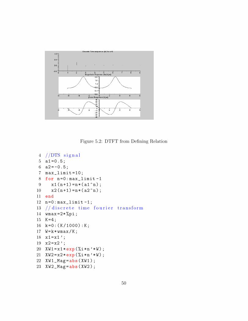
Figure 5.2: DTFT from Defining Relation
4 //DTS s i g n a l5 a1=0.5;
6 a2= -0.5;
7 max_limit =10;
8 for n=0: max_limit -1
9 x1(n+1)=n*(a1^n);
10 x2(n+1)=n*(a2^n);
11 end
12 n=0: max_limit -1;
13 // d i s c r e t e t ime f o u r i e r t r a n s f o r m14 wmax =2*%pi;
15 K=4;
16 k=0:(K/1000):K;
17 W=k*wmax/K;
18 x1=x1 ’;
19 x2=x2 ’;
20 XW1=x1*exp(%i*n’*W);
21 XW2=x2*exp(%i*n’*W);
22 XW1_Mag=abs(XW1);
23 XW2_Mag=abs(XW2);
50
24 W=[- mtlb_fliplr(W),W(2:1001) ]; // omega form25 XW1_Mag =[ mtlb_fliplr(XW1_Mag),XW1_Mag (2:1001) ];
26 XW2_Mag =[ mtlb_fliplr(XW2_Mag),XW2_Mag (2:1001) ];
27 [XW1_phase ,db]= phasemag(XW1);
28 [XW2_phase ,db]= phasemag(XW2);
29 XW1_phase=[- mtlb_fliplr(XW1_phase),XW1_phase (2:1001)
];
30 XW2_phase=[- mtlb_fliplr(XW2_phase),XW2_phase (2:1001)
];
31
32 // p l o t f o r a>033 figure
34 subplot (3,1,1);
35 plot2d3( ’ gnn ’ ,n,x1)36 xtitle( ’ D i s c r e t e t ime sequencex [ n ] a>0 ’ )37 subplot (3,1,2);
38 a=gca();
39 a.y_location=” o r i g i n ”;40 a.x_location=” o r i g i n ”;41 plot2d3(W,XW1_Mag);
42 title( ’ magnitude Response abs ( exp ( jw ) ) ’ )43 subplot (3,1,3);
44 a=gca();
45 a.y_location=” o r i g i n ”;46 a.x_location=” o r i g i n ”;47 plot2d(W,XW1_phase);
48 title( ’ magnitude Response abs ( exp ( jw ) ) ’ )49 // p l o t f o r a<050 figure
51 subplot (3,1,1);
52 plot2d3( ’ gnn ’ ,n,x2);53 xtitle( ’ D i s c r e t e Time s equence x [ n ] f o r a>0 ’ )54 subplot (3,1,2);
55 a=gca();
56 a.y_location=” o r i g i n ”;57 a.x_location=” o r i g i n ”;58 plot2d(W,XW2_Mag);
59 title( ’ Magnitude Response abs (X( jw ) ) ’ )
51

Figure 5.3: Some DTFT pairs using properties
60 subplot (3,1,3);
61 a=gca();
62 a.y_location=” o r i g i n ”;63 a.x_location=” o r i g i n ”;64 plot2d(W,XW2_phase);
65 title( ’ phase Response <(X( jw ) ) ’ )
Scilab code Exa 5.3b Some DTFT pairs using properties
1 //DTFT o f x [ n]=n ∗ ( a ) ˆn∗u [ n ]2 clear;
3 clc;close;
4 //DTS s i g n a l5 a1=0.5;
52
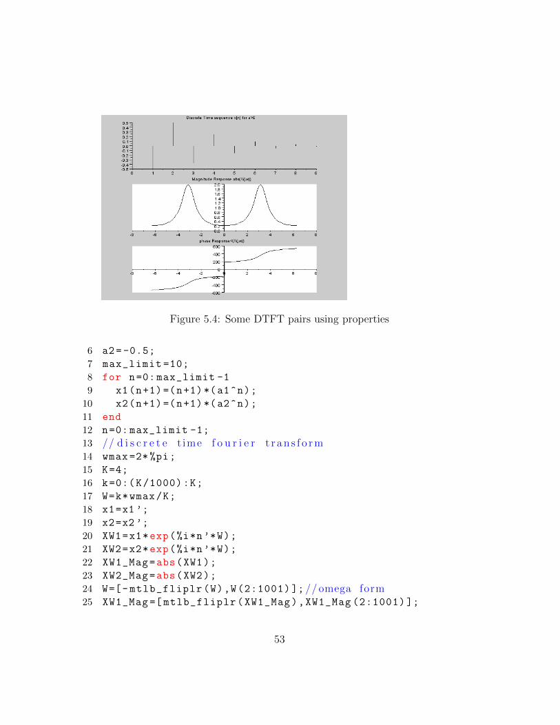
Figure 5.4: Some DTFT pairs using properties
6 a2= -0.5;
7 max_limit =10;
8 for n=0: max_limit -1
9 x1(n+1)=(n+1)*(a1^n);
10 x2(n+1)=(n+1)*(a2^n);
11 end
12 n=0: max_limit -1;
13 // d i s c r e t e t ime f o u r i e r t r a n s f o r m14 wmax =2*%pi;
15 K=4;
16 k=0:(K/1000):K;
17 W=k*wmax/K;
18 x1=x1 ’;
19 x2=x2 ’;
20 XW1=x1*exp(%i*n’*W);
21 XW2=x2*exp(%i*n’*W);
22 XW1_Mag=abs(XW1);
23 XW2_Mag=abs(XW2);
24 W=[- mtlb_fliplr(W),W(2:1001) ]; // omega form25 XW1_Mag =[ mtlb_fliplr(XW1_Mag),XW1_Mag (2:1001) ];
53
26 XW2_Mag =[ mtlb_fliplr(XW2_Mag),XW2_Mag (2:1001) ];
27 [XW1_phase ,db]= phasemag(XW1);
28 [XW2_phase ,db]= phasemag(XW2);
29 XW1_phase=[- mtlb_fliplr(XW1_phase),XW1_phase (2:1001)
];
30 XW2_phase=[- mtlb_fliplr(XW2_phase),XW2_phase (2:1001)
];
31
32 // p l o t f o r a>033 figure
34 subplot (3,1,1);
35 plot2d3( ’ gnn ’ ,n,x1)36 xtitle( ’ D i s c r e t e t ime sequencex [ n ] a>0 ’ )37 subplot (3,1,2);
38 a=gca();
39 a.y_location=” o r i g i n ”;40 a.x_location=” o r i g i n ”;41 plot2d3(W,XW1_Mag);
42 title( ’ magnitude Response abs ( exp ( jw ) ) ’ )43 subplot (3,1,3);
44 a=gca();
45 a.y_location=” o r i g i n ”;46 a.x_location=” o r i g i n ”;47 plot2d(W,XW1_phase);
48 title( ’ magnitude Response abs ( exp ( jw ) ) ’ )49 // p l o t f o r a<050 figure
51 subplot (3,1,1);
52 plot2d3( ’ gnn ’ ,n,x2);53 xtitle( ’ D i s c r e t e Time s equence x [ n ] f o r a>0 ’ )54 subplot (3,1,2);
55 a=gca();
56 a.y_location=” o r i g i n ”;57 a.x_location=” o r i g i n ”;58 plot2d(W,XW2_Mag);
59 title( ’ Magnitude Response abs (X( jw ) ) ’ )60 subplot (3,1,3);
61 a=gca();
54
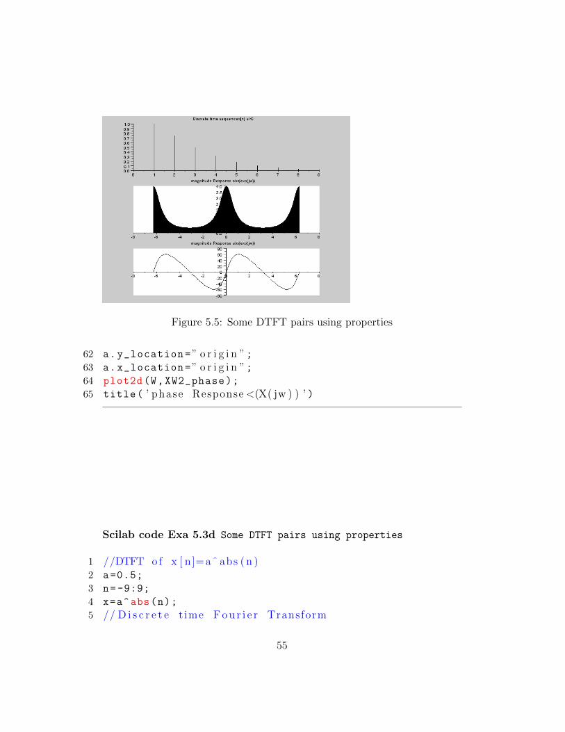
Figure 5.5: Some DTFT pairs using properties
62 a.y_location=” o r i g i n ”;63 a.x_location=” o r i g i n ”;64 plot2d(W,XW2_phase);
65 title( ’ phase Response <(X( jw ) ) ’ )
Scilab code Exa 5.3d Some DTFT pairs using properties
1 //DTFT o f x [ n]=aˆ abs ( n )2 a=0.5;
3 n=-9:9;
4 x=a^abs(n);
5 // D i s c r e t e t ime F o u r i e r Transform
55
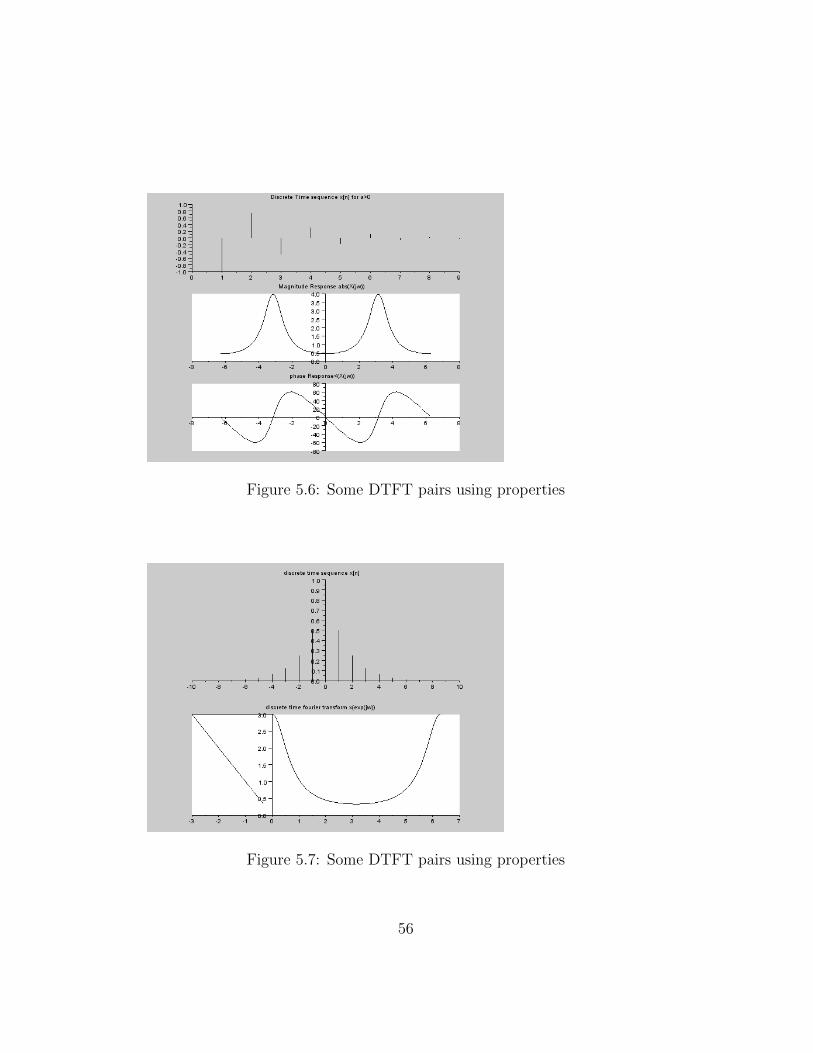
Figure 5.6: Some DTFT pairs using properties
Figure 5.7: Some DTFT pairs using properties
56
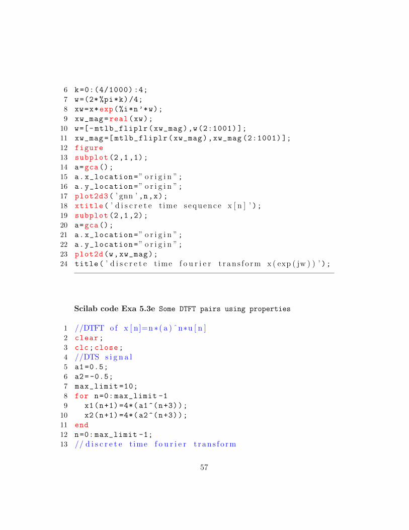
6 k=0:(4/1000) :4;
7 w=(2* %pi*k)/4;
8 xw=x*exp(%i*n’*w);
9 xw_mag=real(xw);
10 w=[- mtlb_fliplr(xw_mag),w(2:1001) ];
11 xw_mag =[ mtlb_fliplr(xw_mag),xw_mag (2:1001) ];
12 figure
13 subplot (2,1,1);
14 a=gca();
15 a.x_location=” o r i g i n ”;16 a.y_location=” o r i g i n ”;17 plot2d3( ’ gnn ’ ,n,x);18 xtitle( ’ d i s c r e t e t ime s equence x [ n ] ’ );19 subplot (2,1,2);
20 a=gca();
21 a.x_location=” o r i g i n ”;22 a.y_location=” o r i g i n ”;23 plot2d(w,xw_mag);
24 title( ’ d i s c r e t e t ime f o u r i e r t r a n s f o r m x ( exp ( jw ) ) ’ );
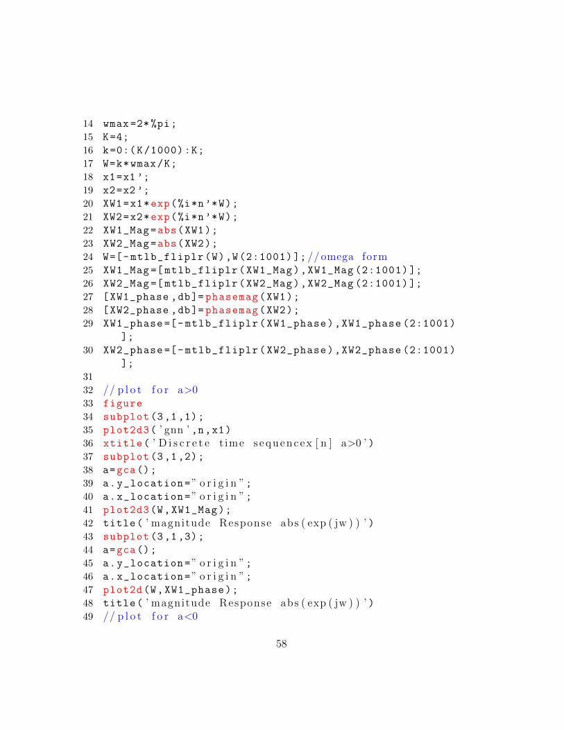
Scilab code Exa 5.3e Some DTFT pairs using properties
1 //DTFT o f x [ n]=n ∗ ( a ) ˆn∗u [ n ]2 clear;
3 clc;close;
4 //DTS s i g n a l5 a1=0.5;
6 a2= -0.5;
7 max_limit =10;
8 for n=0: max_limit -1
9 x1(n+1) =4*(a1^(n+3));
10 x2(n+1) =4*(a2^(n+3));
11 end
12 n=0: max_limit -1;
13 // d i s c r e t e t ime f o u r i e r t r a n s f o r m
57
14 wmax =2*%pi;
15 K=4;
16 k=0:(K/1000):K;
17 W=k*wmax/K;
18 x1=x1 ’;
19 x2=x2 ’;
20 XW1=x1*exp(%i*n’*W);
21 XW2=x2*exp(%i*n’*W);
22 XW1_Mag=abs(XW1);
23 XW2_Mag=abs(XW2);
24 W=[- mtlb_fliplr(W),W(2:1001) ]; // omega form25 XW1_Mag =[ mtlb_fliplr(XW1_Mag),XW1_Mag (2:1001) ];
26 XW2_Mag =[ mtlb_fliplr(XW2_Mag),XW2_Mag (2:1001) ];
27 [XW1_phase ,db]= phasemag(XW1);
28 [XW2_phase ,db]= phasemag(XW2);
29 XW1_phase=[- mtlb_fliplr(XW1_phase),XW1_phase (2:1001)
];
30 XW2_phase=[- mtlb_fliplr(XW2_phase),XW2_phase (2:1001)
];
31
32 // p l o t f o r a>033 figure
34 subplot (3,1,1);
35 plot2d3( ’ gnn ’ ,n,x1)36 xtitle( ’ D i s c r e t e t ime sequencex [ n ] a>0 ’ )37 subplot (3,1,2);
38 a=gca();
39 a.y_location=” o r i g i n ”;40 a.x_location=” o r i g i n ”;41 plot2d3(W,XW1_Mag);
42 title( ’ magnitude Response abs ( exp ( jw ) ) ’ )43 subplot (3,1,3);
44 a=gca();
45 a.y_location=” o r i g i n ”;46 a.x_location=” o r i g i n ”;47 plot2d(W,XW1_phase);
48 title( ’ magnitude Response abs ( exp ( jw ) ) ’ )49 // p l o t f o r a<0
58

Figure 5.8: Some DTFT pairs using properties
50 figure
51 subplot (3,1,1);
52 plot2d3( ’ gnn ’ ,n,x2);53 xtitle( ’ D i s c r e t e Time s equence x [ n ] f o r a>0 ’ )54 subplot (3,1,2);
55 a=gca();
56 a.y_location=” o r i g i n ”;57 a.x_location=” o r i g i n ”;58 plot2d(W,XW2_Mag);
59 title( ’ Magnitude Response abs (X( jw ) ) ’ )60 subplot (3,1,3);
61 a=gca();
62 a.y_location=” o r i g i n ”;63 a.x_location=” o r i g i n ”;64 plot2d(W,XW2_phase);
65 title( ’ phase Response <(X( jw ) ) ’ )
59
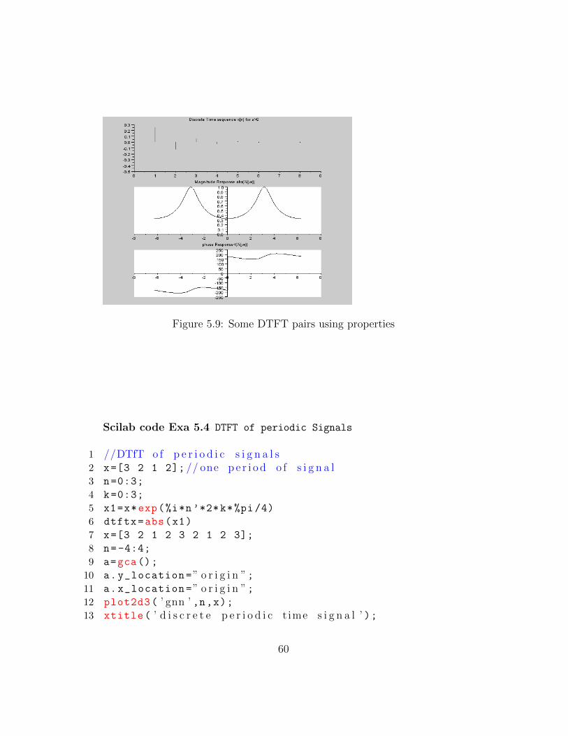
Figure 5.9: Some DTFT pairs using properties
Scilab code Exa 5.4 DTFT of periodic Signals
1 //DTfT o f p e r i o d i c s i g n a l s2 x=[3 2 1 2]; // one p e r i o d o f s i g n a l3 n=0:3;
4 k=0:3;
5 x1=x*exp(%i*n’*2*k*%pi /4)
6 dtftx=abs(x1)
7 x=[3 2 1 2 3 2 1 2 3];
8 n=-4:4;
9 a=gca();
10 a.y_location=” o r i g i n ”;11 a.x_location=” o r i g i n ”;12 plot2d3( ’ gnn ’ ,n,x);13 xtitle( ’ d i s c r e t e p e r i o d i c t ime s i g n a l ’ );
60
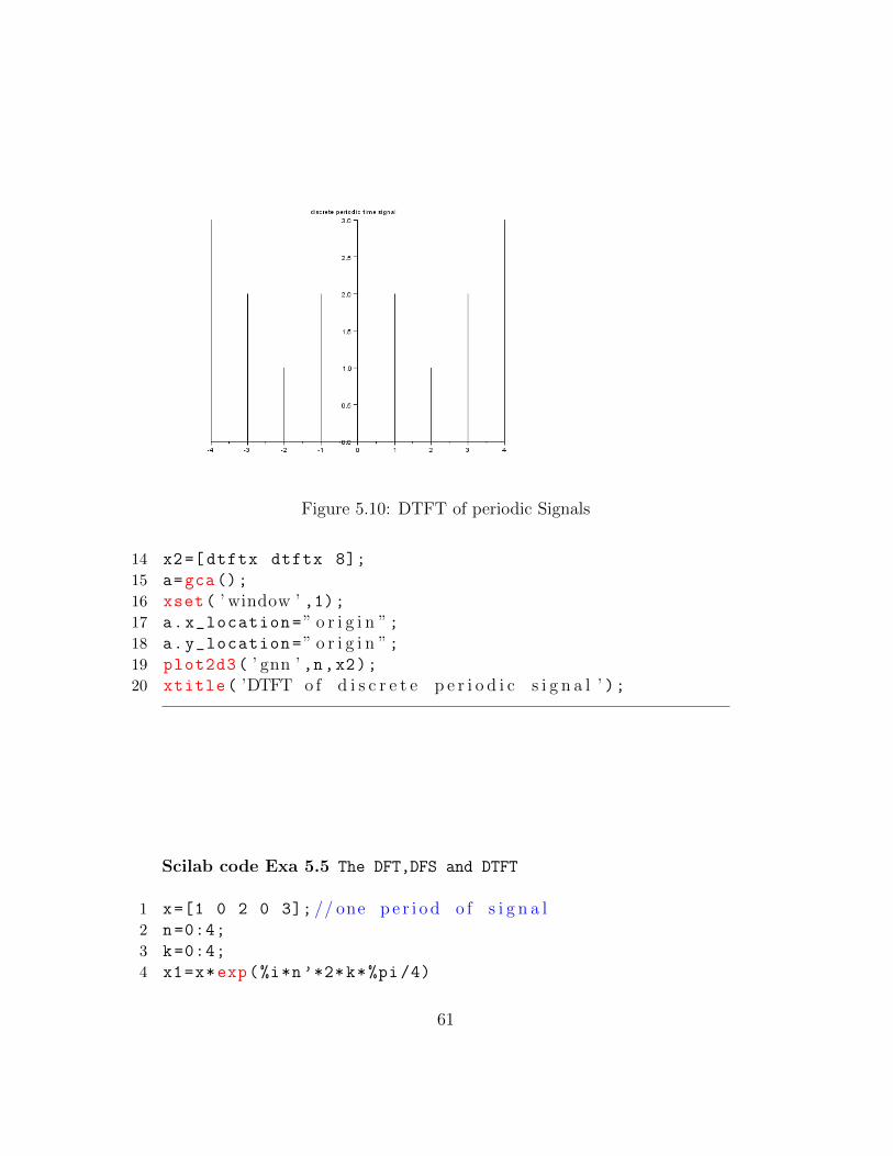
Figure 5.10: DTFT of periodic Signals
14 x2=[ dtftx dtftx 8];
15 a=gca();
16 xset( ’ window ’ ,1);17 a.x_location=” o r i g i n ”;18 a.y_location=” o r i g i n ”;19 plot2d3( ’ gnn ’ ,n,x2);20 xtitle( ’DTFT o f d i s c r e t e p e r i o d i c s i g n a l ’ );
Scilab code Exa 5.5 The DFT,DFS and DTFT
1 x=[1 0 2 0 3]; // one p e r i o d o f s i g n a l2 n=0:4;
3 k=0:4;
4 x1=x*exp(%i*n’*2*k*%pi/4)
61
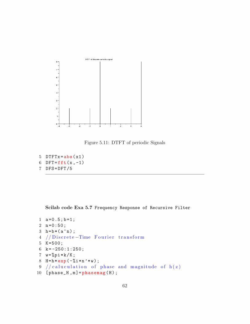
Figure 5.11: DTFT of periodic Signals
5 DTFTx=abs(x1)
6 DFT=fft(x,-1)
7 DFS=DFT/5
Scilab code Exa 5.7 Frequency Response of Recursive Filter
1 a=0.5;b=1;
2 n=0:50;
3 h=b*(a^n);
4 // D i s c r e t e −Time F o u r i e r t r a n s f o r m5 K=500;
6 k= -250:1:250;
7 w=%pi*k/K;
8 H=h*exp(-%i*n’*w);
9 // c a l u c u l a t i o n o f phase and magnitude o f h ( z )10 [phase_H ,m]= phasemag(H);
62
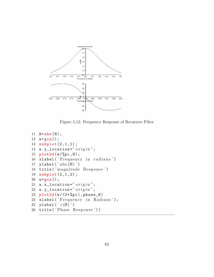
Figure 5.12: Frequency Response of Recursive Filter
11 H=abs(H);
12 a=gca();
13 subplot (2,1,1);
14 a.y_location=” o r i g i n ”;15 plot2d(w/%pi ,H);
16 xlabel( ’ Frequency i n r a d i a n s ’ )17 ylabel( ’ abs (H) ’ )18 title( ’ magnitude Response ’ )19 subplot (2,1,2);
20 a=gca();
21 a.x_location=” o r i g i n ”;22 a.y_location=” o r i g i n ”;23 plot2d(w/(2* %pi),phase_H)
24 xlabel( ’ Frequency i n Radians ’ );25 ylabel( ’<(H) ’ )26 title( ’ Phase Response ’ ))
63
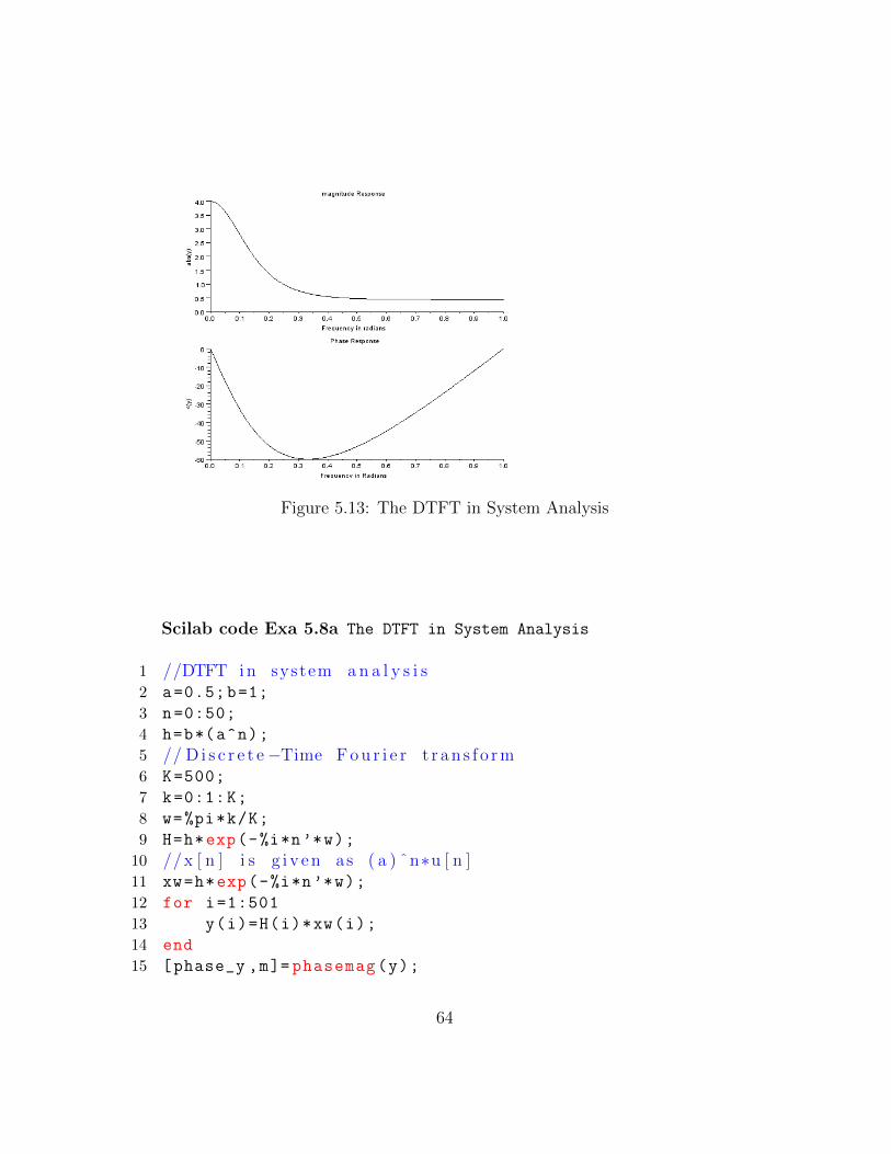
Figure 5.13: The DTFT in System Analysis
Scilab code Exa 5.8a The DTFT in System Analysis
1 //DTFT i n system a n a l y s i s2 a=0.5;b=1;
3 n=0:50;
4 h=b*(a^n);
5 // D i s c r e t e −Time F o u r i e r t r a n s f o r m6 K=500;
7 k=0:1:K;
8 w=%pi*k/K;
9 H=h*exp(-%i*n’*w);
10 //x [ n ] i s g i v e n as ( a ) ˆn∗u [ n ]11 xw=h*exp(-%i*n’*w);
12 for i=1:501
13 y(i)=H(i)*xw(i);
14 end
15 [phase_y ,m]= phasemag(y);
64
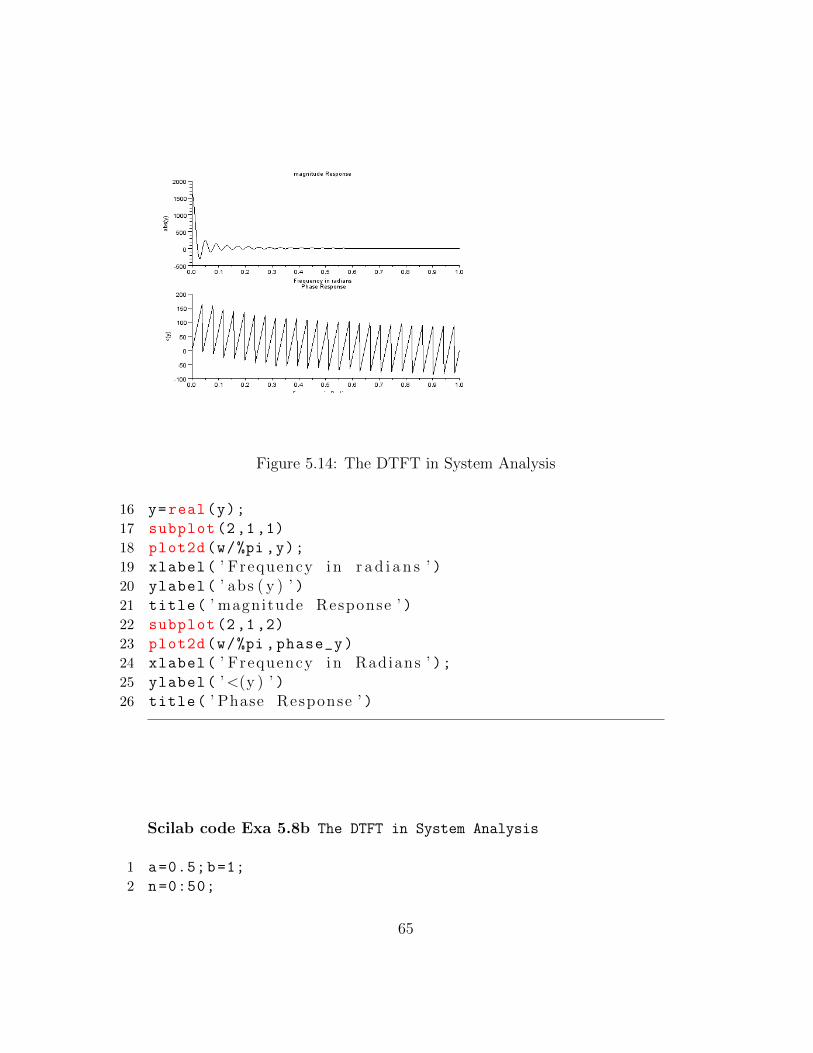
Figure 5.14: The DTFT in System Analysis
16 y=real(y);
17 subplot (2,1,1)
18 plot2d(w/%pi ,y);
19 xlabel( ’ Frequency i n r a d i a n s ’ )20 ylabel( ’ abs ( y ) ’ )21 title( ’ magnitude Response ’ )22 subplot (2,1,2)
23 plot2d(w/%pi ,phase_y)
24 xlabel( ’ Frequency i n Radians ’ );25 ylabel( ’<(y ) ’ )26 title( ’ Phase Response ’ )
Scilab code Exa 5.8b The DTFT in System Analysis
1 a=0.5;b=1;
2 n=0:50;
65

3 h=4*(a^n);
4 // D i s c r e t e −Time F o u r i e r t r a n s f o r m5 K=500;
6 k=0:1:K;
7 w=%pi*k/K;
8 H=h*exp(-%i*n’*w);
9 //x [ n ] i s g i v e n as ( a ) ˆn∗u [ n ]10 x=4*[ ones (1:51) ];
11 xw=x*exp(%i*n’*w);
12 for i=1:501
13 y(i)=H(i)*xw(i);
14 end
15 [phase_y ,m]= phasemag(y);
16 y=real(y);
17 subplot (2,1,1);
18 plot2d(w/%pi ,y);
19 xlabel( ’ Frequency i n r a d i a n s ’ )20 ylabel( ’ abs ( y ) ’ )21 title( ’ magnitude Response ’ )22 subplot (2,1,2)
23 plot2d(w/%pi ,phase_y)
24 xlabel( ’ Frequency i n Radians ’ );25 ylabel( ’<(y ) ’ )26 title( ’ Phase Response ’ )
Scilab code Exa 5.9a DTFT and steady state response
1 //DTFT and s t e ady s t a t e r e s p o n s e2 a=0.5,b=1;F=0.25;
3 n=0:(5/1000) :5;
4 h=(a^n);
5 x=10* cos (0.5* %pi*n’+%pi /3);
6 H=h*exp(-%i*n’*F);
66
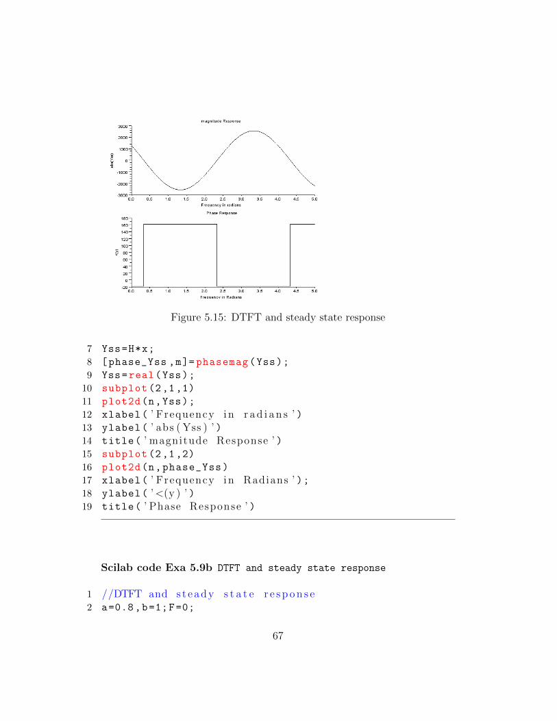
Figure 5.15: DTFT and steady state response
7 Yss=H*x;
8 [phase_Yss ,m]= phasemag(Yss);
9 Yss=real(Yss);
10 subplot (2,1,1)
11 plot2d(n,Yss);
12 xlabel( ’ Frequency i n r a d i a n s ’ )13 ylabel( ’ abs ( Yss ) ’ )14 title( ’ magnitude Response ’ )15 subplot (2,1,2)
16 plot2d(n,phase_Yss)
17 xlabel( ’ Frequency i n Radians ’ );18 ylabel( ’<(y ) ’ )19 title( ’ Phase Response ’ )
Scilab code Exa 5.9b DTFT and steady state response
1 //DTFT and s t e ady s t a t e r e s p o n s e2 a=0.8,b=1;F=0;
67
3 n=0:50;
4 h=(a^n);
5 x=4*[ ones (1:10) ];
6 H=h*exp(-%i*n’*F)
7 Yss=H*x
Scilab code Exa 5.10a System Representation in various forms
1 // System R e p r e s e n t a t i o n i n v a r i o u s forms2 a=0.8;b=2;
3 n=0:50;
4 h=b*(a^n);
5 // D i s c r e t e −Time F o u r i e r t r a n s f o r m6 K=500;
7 k=0:1:K;
8 w=%pi*k/K;
9 H=h*exp(-%i*n’*w);
10 // c a l u c u l a t i o n o f phase and magnitude o f h ( z )11 [phase_H ,m]= phasemag(H);
12 H=abs(H);
13 subplot (2,1,1);
14 plot2d(w/%pi ,H);
15 xlabel( ’ Frequency i n r a d i a n s ’ )16 ylabel( ’ abs (H) ’ )17 title( ’ magnitude Response ’ )18 subplot (2,1,2)
19 plot2d(w/%pi ,phase_H)
20 xlabel( ’ Frequency i n Radians ’ );21 ylabel( ’<(H) ’ )22 title( ’ Phase Response ’ )
68
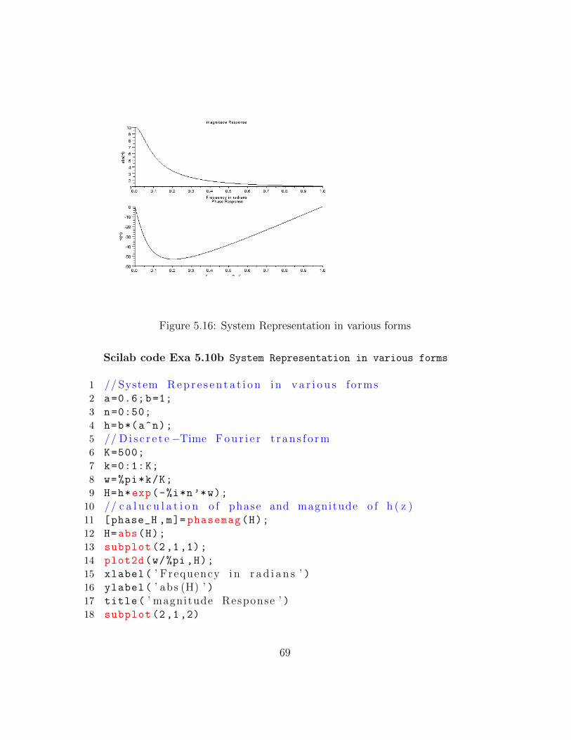
Figure 5.16: System Representation in various forms
Scilab code Exa 5.10b System Representation in various forms
1 // System R e p r e s e n t a t i o n i n v a r i o u s forms2 a=0.6;b=1;
3 n=0:50;
4 h=b*(a^n);
5 // D i s c r e t e −Time F o u r i e r t r a n s f o r m6 K=500;
7 k=0:1:K;
8 w=%pi*k/K;
9 H=h*exp(-%i*n’*w);
10 // c a l u c u l a t i o n o f phase and magnitude o f h ( z )11 [phase_H ,m]= phasemag(H);
12 H=abs(H);
13 subplot (2,1,1);
14 plot2d(w/%pi ,H);
15 xlabel( ’ Frequency i n r a d i a n s ’ )16 ylabel( ’ abs (H) ’ )17 title( ’ magnitude Response ’ )18 subplot (2,1,2)
69
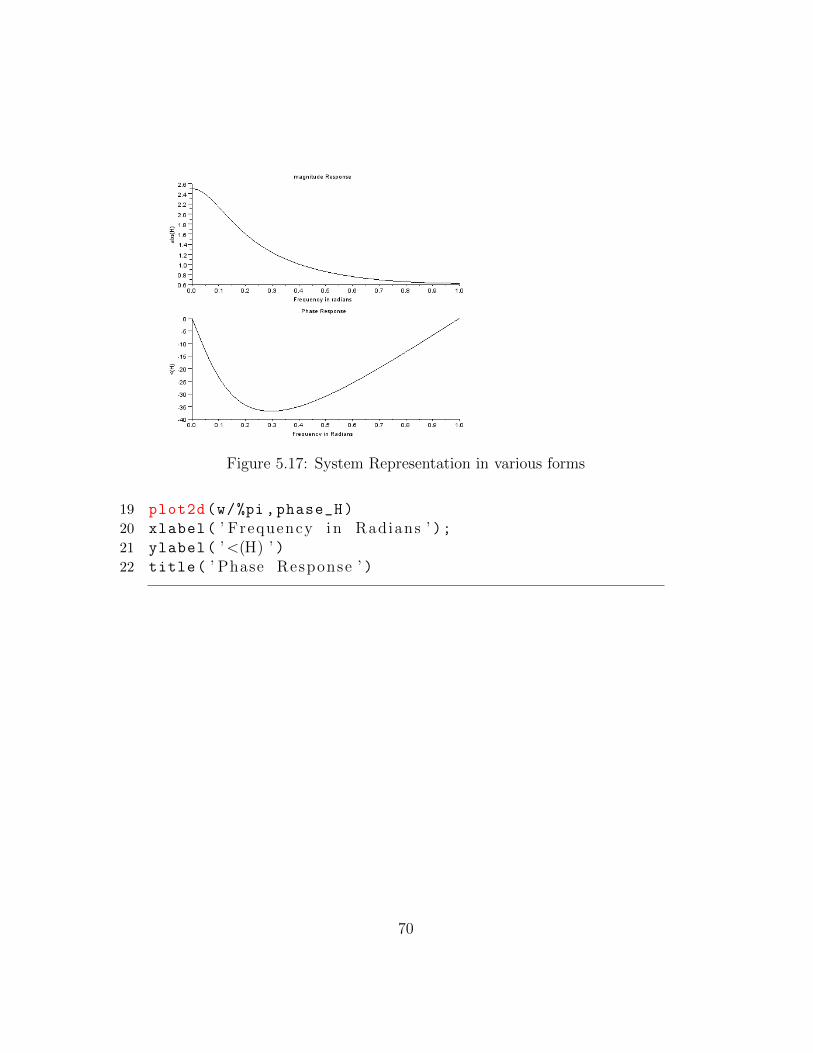
Figure 5.17: System Representation in various forms
19 plot2d(w/%pi ,phase_H)
20 xlabel( ’ Frequency i n Radians ’ );21 ylabel( ’<(H) ’ )22 title( ’ Phase Response ’ )
70
Chapter 6
Filter Concepts
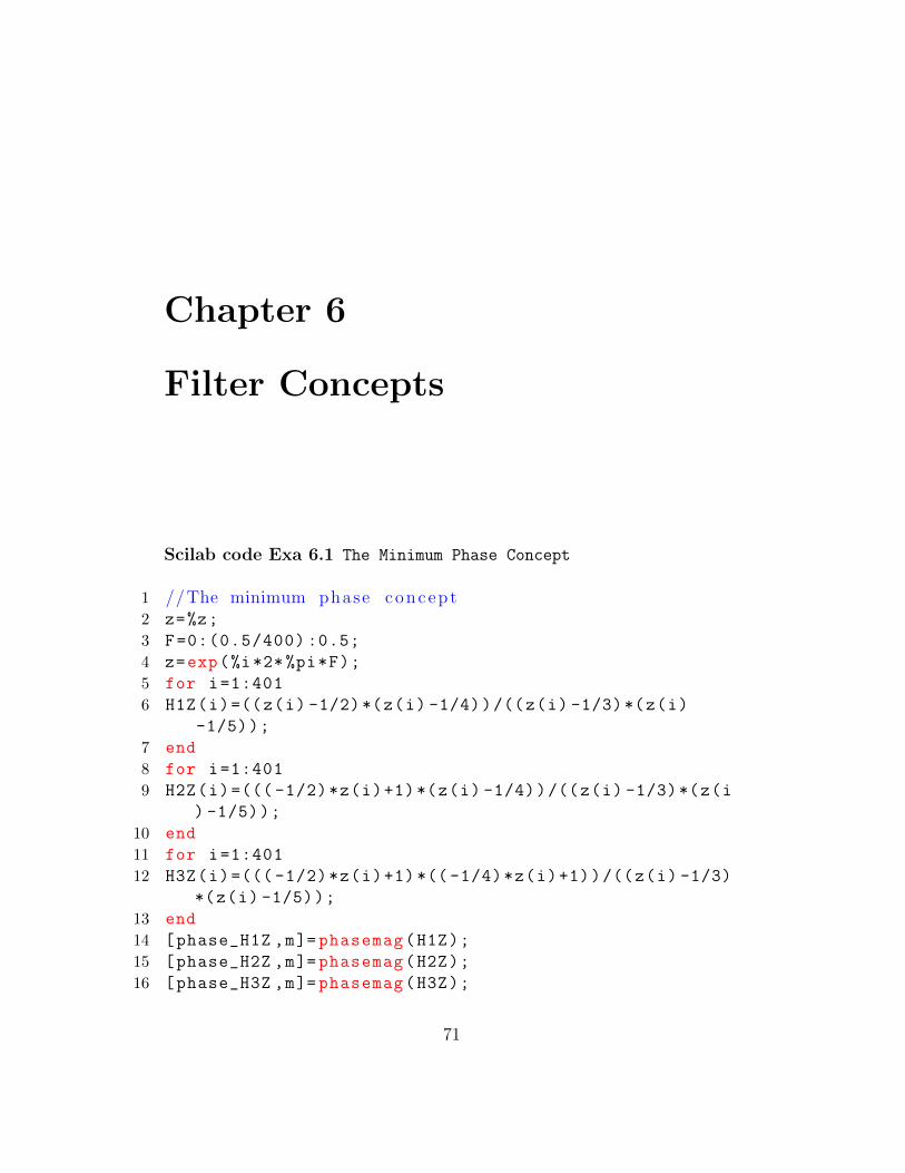
Scilab code Exa 6.1 The Minimum Phase Concept
1 //The minimum phase concep t2 z=%z;
3 F=0:(0.5/400) :0.5;
4 z=exp(%i*2* %pi*F);
5 for i=1:401
6 H1Z(i)=((z(i) -1/2)*(z(i) -1/4))/((z(i) -1/3)*(z(i)
-1/5));
7 end
8 for i=1:401
9 H2Z(i)=((( -1/2)*z(i)+1)*(z(i) -1/4))/((z(i) -1/3)*(z(i
) -1/5));
10 end
11 for i=1:401
12 H3Z(i)=((( -1/2)*z(i)+1) *(( -1/4)*z(i)+1))/((z(i) -1/3)
*(z(i) -1/5));
13 end
14 [phase_H1Z ,m]= phasemag(H1Z);
15 [phase_H2Z ,m]= phasemag(H2Z);
16 [phase_H3Z ,m]= phasemag(H3Z);
71
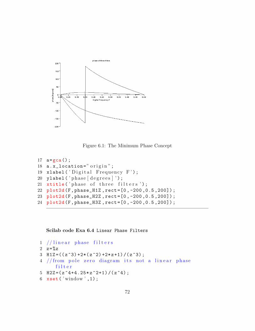
Figure 6.1: The Minimum Phase Concept
17 a=gca();
18 a.x_location=” o r i g i n ”;19 xlabel( ’ D i g i t a l Frequency F ’ );20 ylabel( ’ phase [ d e g r e e s ] ’ );21 xtitle( ’ phase o f t h r e e f i l t e r s ’ );22 plot2d(F,phase_H1Z ,rect =[0 , -200 ,0.5 ,200]);
23 plot2d(F,phase_H2Z ,rect =[0 , -200 ,0.5 ,200]);
24 plot2d(F,phase_H3Z ,rect =[0 , -200 ,0.5 ,200]);
Scilab code Exa 6.4 Linear Phase Filters
1 // l i n e a r phase f i l t e r s2 z=%z
3 H1Z =((z^3) +2*(z^2)+2*z+1)/(z^3);
4 // from p o l e z e r o diagram i t s not a l i n e a r phasef i l t e r
5 H2Z=(z^4+4.25*z^2+1) /(z^4);
6 xset( ’ window ’ ,1);
72
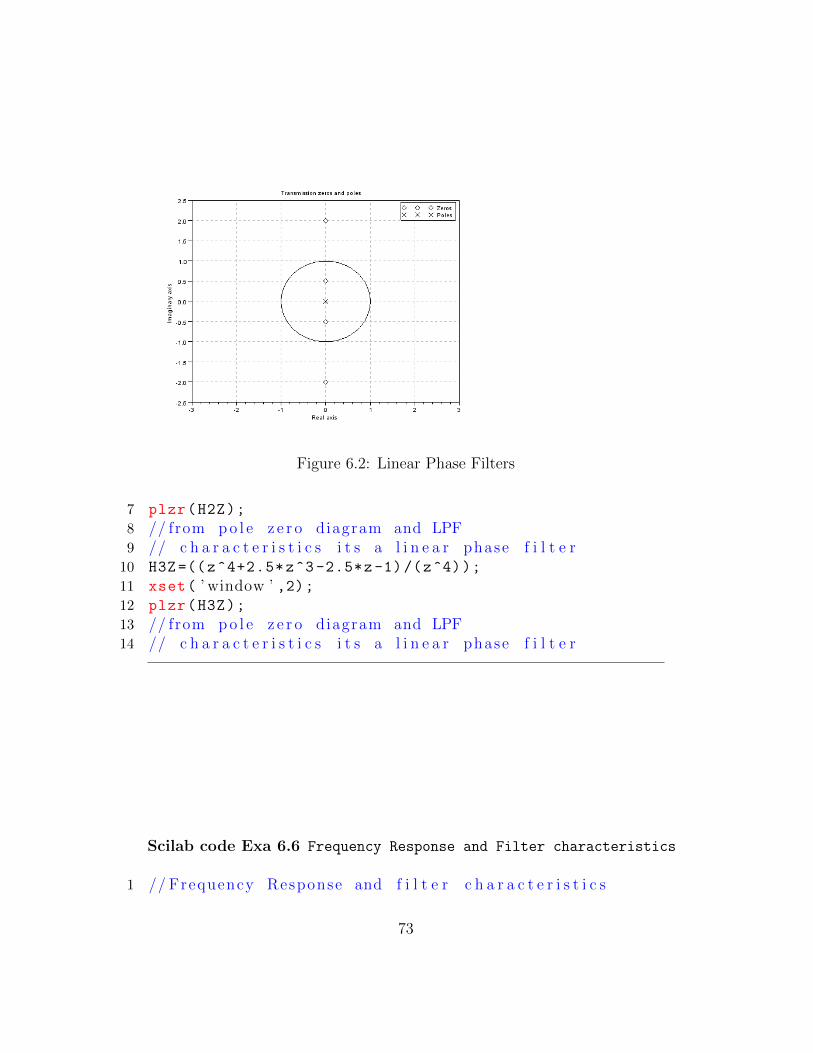
Figure 6.2: Linear Phase Filters
7 plzr(H2Z);
8 // from p o l e z e r o diagram and LPF9 // c h a r a c t e r i s t i c s i t s a l i n e a r phase f i l t e r10 H3Z =((z^4+2.5*z^3 -2.5*z-1)/(z^4));
11 xset( ’ window ’ ,2);12 plzr(H3Z);
13 // from p o l e z e r o diagram and LPF14 // c h a r a c t e r i s t i c s i t s a l i n e a r phase f i l t e r
Scilab code Exa 6.6 Frequency Response and Filter characteristics
1 // Frequency Response and f i l t e r c h a r a c t e r i s t i c s
73
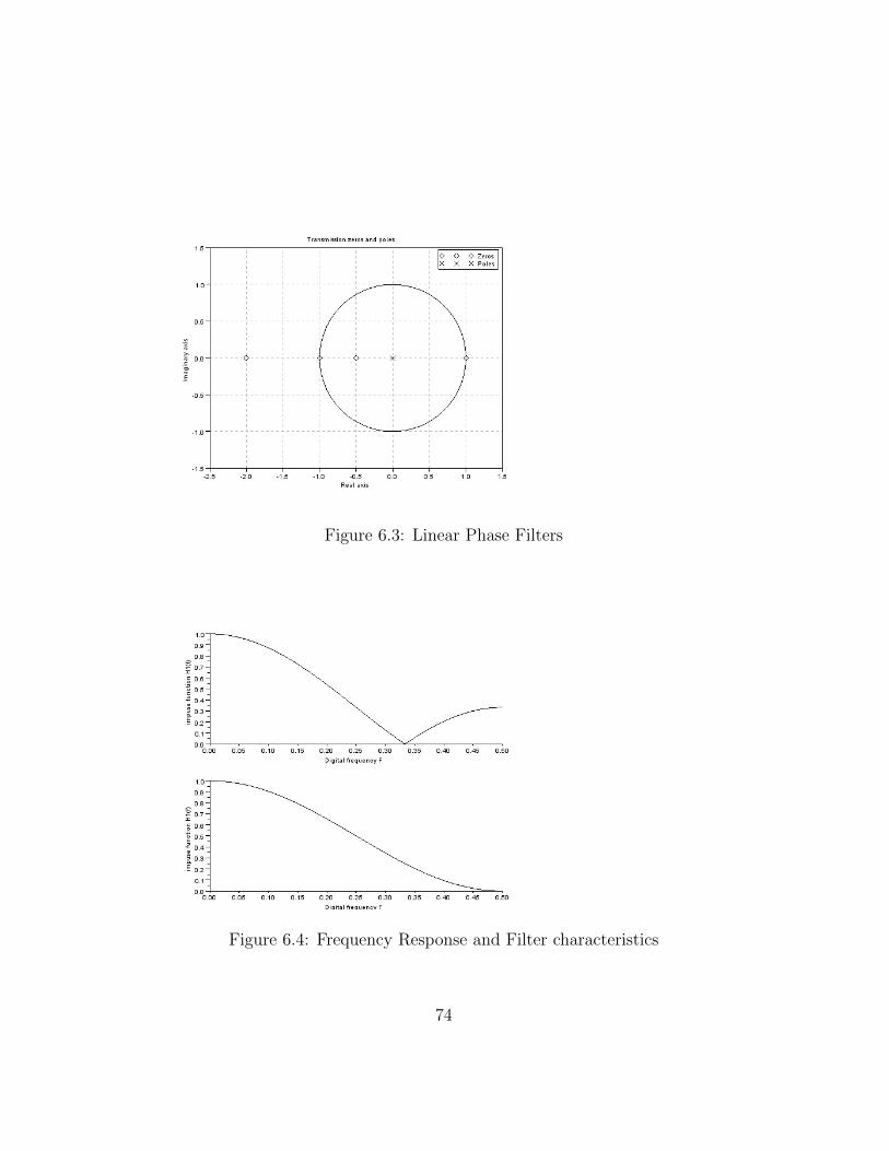
Figure 6.3: Linear Phase Filters
Figure 6.4: Frequency Response and Filter characteristics
74
2 z=%z;
3 F=0:(0.5/200) :0.5;
4 z=exp(%i*2* %pi*F);
5 H1 =(1/3) *(z+1+z^-1);
6 H2=(z/4) +(1/2) +(1/4) *(z^-1);
7 H1=abs(H1);
8 H2=abs(H2);
9 a=gca();
10 a.x_location=” o r i g i n ”;11 subplot (211);
12 plot2d(F,H1);
13 xlabel( ’ D i g i t a l f r e q u e n c y F ’ );14 ylabel( ’ impuse f u n c t i o n H1( f ) ’ );15 subplot (212);
16 plot2d(F,H2);
17 xlabel( ’ D i g i t a l f r e q u e n c y F ’ );18 ylabel( ’ impuse f u n c t i o n H1( f ) ’ );
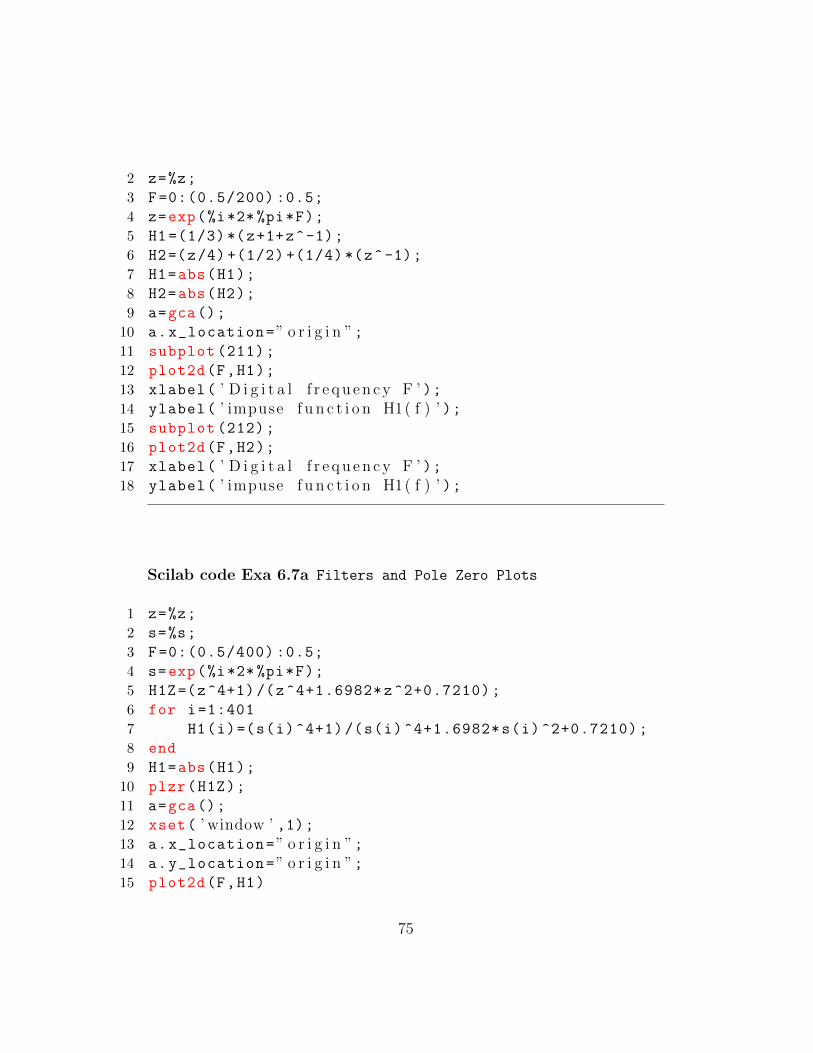
Scilab code Exa 6.7a Filters and Pole Zero Plots
1 z=%z;
2 s=%s;
3 F=0:(0.5/400) :0.5;
4 s=exp(%i*2* %pi*F);
5 H1Z=(z^4+1)/(z^4+1.6982*z^2+0.7210);
6 for i=1:401
7 H1(i)=(s(i)^4+1)/(s(i)^4+1.6982*s(i)^2+0.7210);
8 end
9 H1=abs(H1);
10 plzr(H1Z);
11 a=gca();
12 xset( ’ window ’ ,1);13 a.x_location=” o r i g i n ”;14 a.y_location=” o r i g i n ”;15 plot2d(F,H1)
75
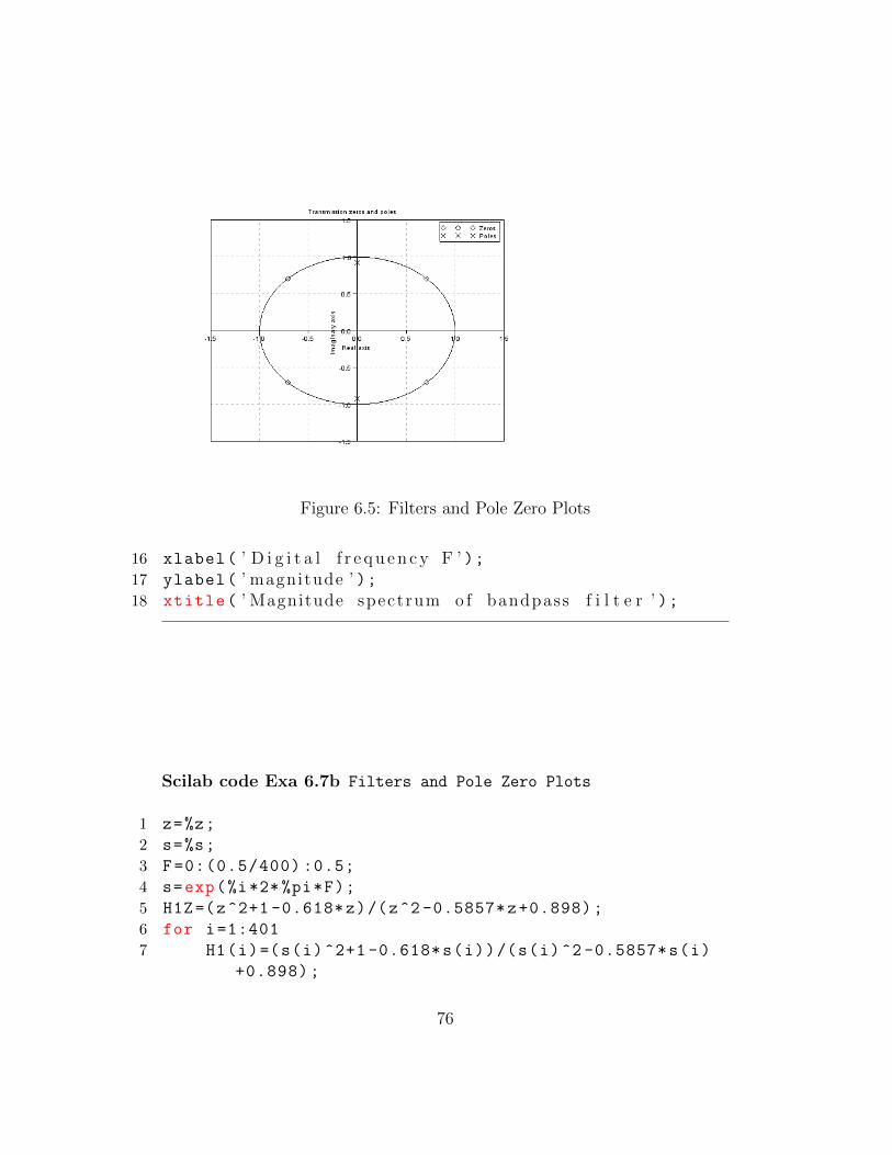
Figure 6.5: Filters and Pole Zero Plots
16 xlabel( ’ D i g i t a l f r e q u e n c y F ’ );17 ylabel( ’ magnitude ’ );18 xtitle( ’ Magnitude spectrum o f bandpass f i l t e r ’ );
Scilab code Exa 6.7b Filters and Pole Zero Plots
1 z=%z;
2 s=%s;
3 F=0:(0.5/400) :0.5;
4 s=exp(%i*2* %pi*F);
5 H1Z=(z^2+1 -0.618*z)/(z^2 -0.5857*z+0.898);
6 for i=1:401
7 H1(i)=(s(i)^2+1 -0.618*s(i))/(s(i)^2 -0.5857*s(i)
+0.898);
76
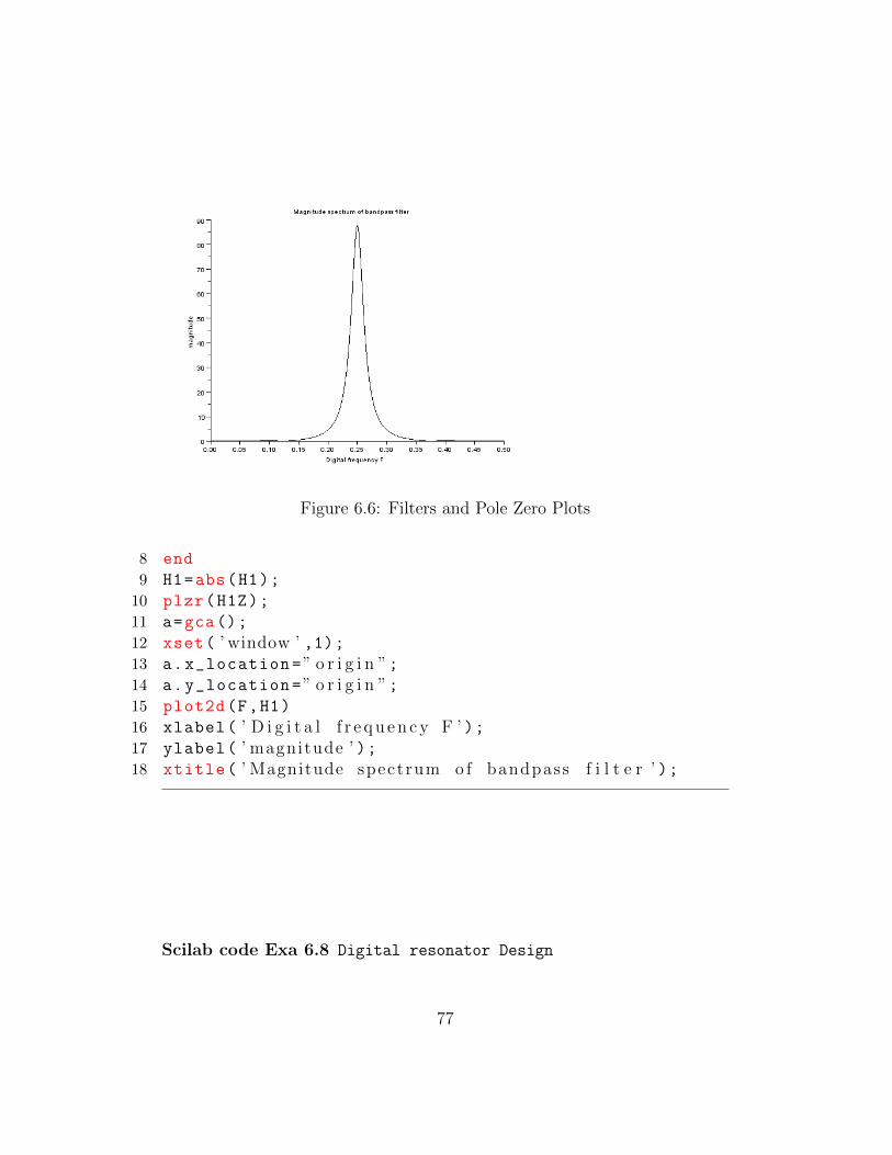
Figure 6.6: Filters and Pole Zero Plots
8 end
9 H1=abs(H1);
10 plzr(H1Z);
11 a=gca();
12 xset( ’ window ’ ,1);13 a.x_location=” o r i g i n ”;14 a.y_location=” o r i g i n ”;15 plot2d(F,H1)
16 xlabel( ’ D i g i t a l f r e q u e n c y F ’ );17 ylabel( ’ magnitude ’ );18 xtitle( ’ Magnitude spectrum o f bandpass f i l t e r ’ );
Scilab code Exa 6.8 Digital resonator Design
77
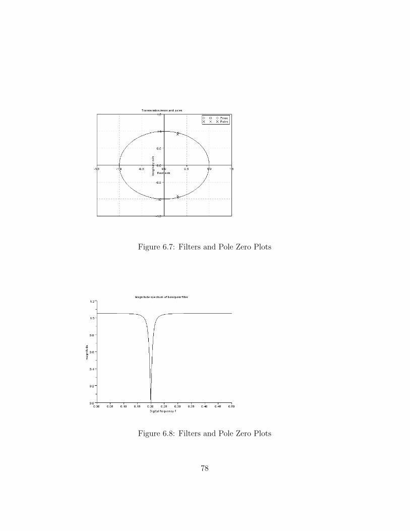
Figure 6.7: Filters and Pole Zero Plots
Figure 6.8: Filters and Pole Zero Plots
78
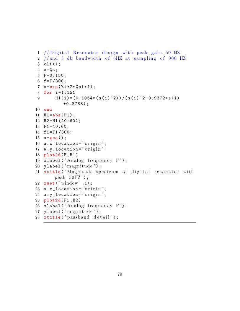
1 // D i g i t a l Resonator d e s i g n with peak ga in 50 HZ2 // and 3 db bandwidth o f 6HZ at sampl ing o f 300 HZ3 clf();
4 s=%s;
5 F=0:150;
6 f=F/300;
7 s=exp(%i*2* %pi*f);
8 for i=1:151
9 H1(i)=(0.1054*(s(i)^2))/(s(i)^2 -0.9372*s(i)
+0.8783);
10 end
11 H1=abs(H1);
12 H2=H1 (40:60);
13 F1 =40:60;
14 f1=F1 /300;
15 a=gca();
16 a.x_location=” o r i g i n ”;17 a.y_location=” o r i g i n ”;18 plot2d(F,H1)
19 xlabel( ’ Analog f r e q u e n c y F ’ );20 ylabel( ’ magnitude ’ );21 xtitle( ’ Magnitude spectrum o f d i g i t a l r e s o n a t o r with
peak 50HZ ’ );22 xset( ’ window ’ ,1);23 a.x_location=” o r i g i n ”;24 a.y_location=” o r i g i n ”;25 plot2d(F1,H2)
26 xlabel( ’ Analog f r e q u e n c y F ’ );27 ylabel( ’ magnitude ’ );28 xtitle( ’ passband d e t a i l ’ );
79
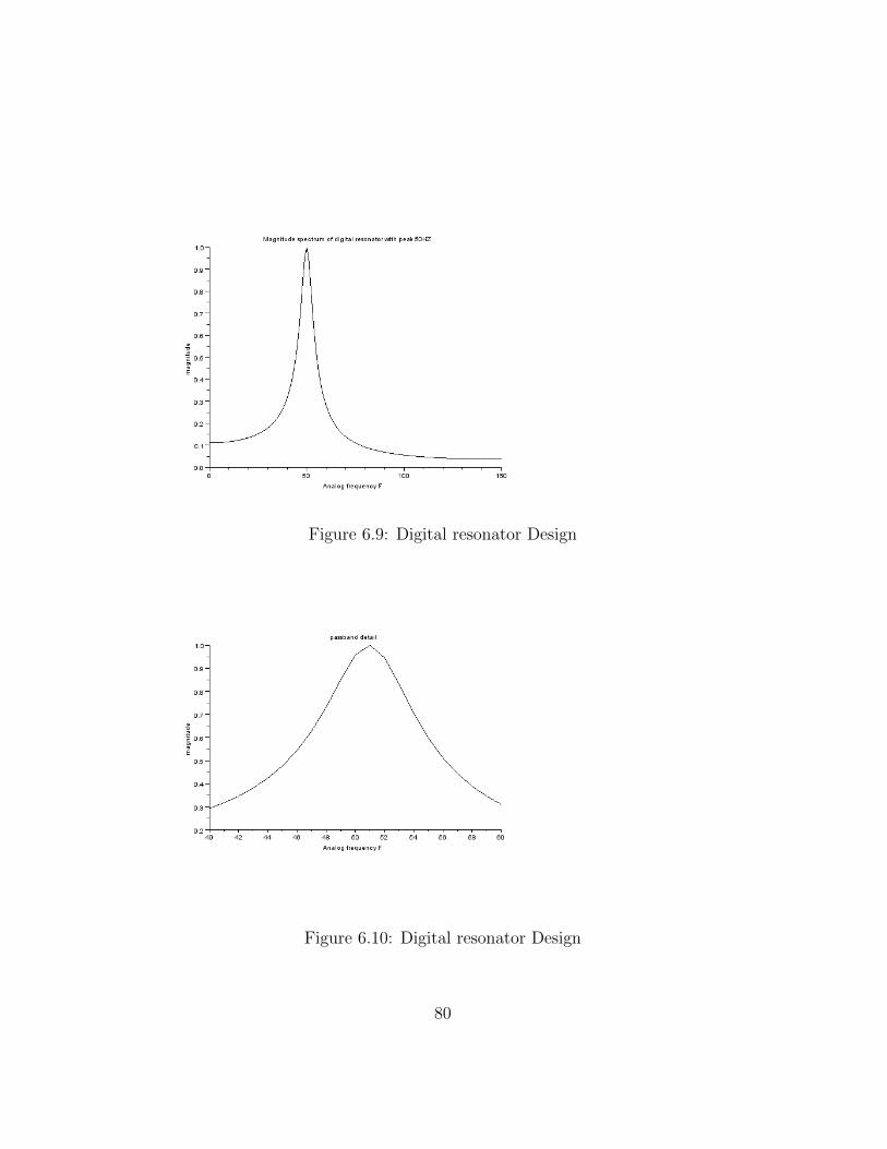
Figure 6.9: Digital resonator Design
Figure 6.10: Digital resonator Design
80
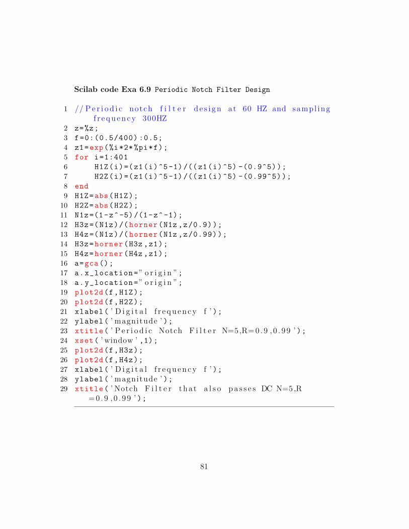
Scilab code Exa 6.9 Periodic Notch Filter Design
1 // P e r i o d i c notch f i l t e r d e s i g n at 60 HZ and sampl ingf r e q u e n c y 300HZ
2 z=%z;
3 f=0:(0.5/400) :0.5;
4 z1=exp(%i*2*%pi*f);
5 for i=1:401
6 H1Z(i)=(z1(i)^5-1)/((z1(i)^5) -(0.9^5));
7 H2Z(i)=(z1(i)^5-1)/((z1(i)^5) -(0.99^5));
8 end
9 H1Z=abs(H1Z);
10 H2Z=abs(H2Z);
11 N1z=(1-z^-5)/(1-z^-1);
12 H3z=(N1z)/( horner(N1z ,z/0.9));
13 H4z=(N1z)/( horner(N1z ,z/0.99));
14 H3z=horner(H3z ,z1);
15 H4z=horner(H4z ,z1);
16 a=gca();
17 a.x_location=” o r i g i n ”;18 a.y_location=” o r i g i n ”;19 plot2d(f,H1Z);
20 plot2d(f,H2Z);
21 xlabel( ’ D i g i t a l f r e q u e n c y f ’ );22 ylabel( ’ magnitude ’ );23 xtitle( ’ P e r i o d i c Notch F i l t e r N=5 ,R= 0 . 9 , 0 . 9 9 ’ );24 xset( ’ window ’ ,1);25 plot2d(f,H3z);
26 plot2d(f,H4z);
27 xlabel( ’ D i g i t a l f r e q u e n c y f ’ );28 ylabel( ’ magnitude ’ );29 xtitle( ’ Notch F i l t e r tha t a l s o p a s s e s DC N=5,R
= 0 . 9 , 0 . 9 9 ’ );
81
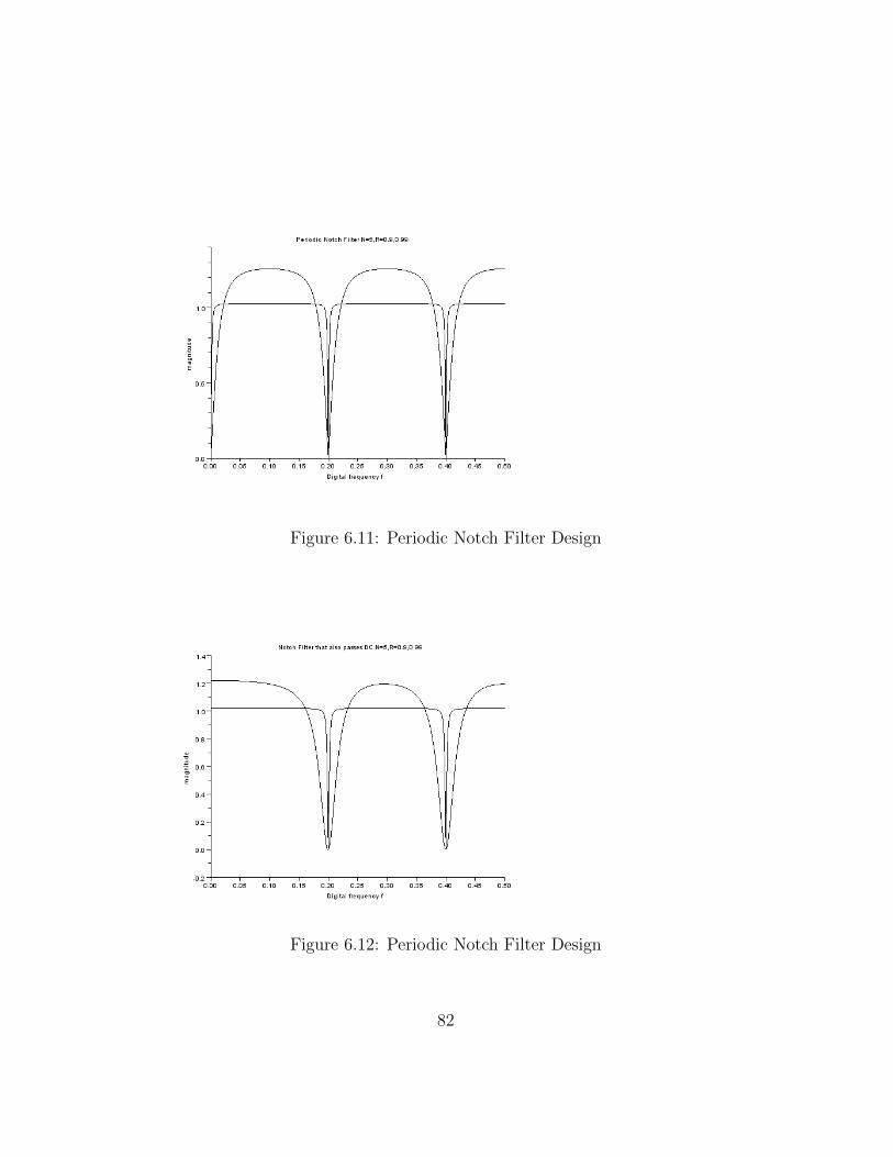
Figure 6.11: Periodic Notch Filter Design
Figure 6.12: Periodic Notch Filter Design
82
Chapter 7
Digital Processing of AnalogSignals
Scilab code Exa 7.3 Sampling oscilloscope
1 // Sampl ing O s c i l l o s c o p e Concepts2 fo=100;a=50;
3 s=(a-1)*fo/a;
4 B=100-s;
5 i=s/(2*B);
6 i=ceil(i);
7 disp(i, ’ The sampl ing f r e q u e n c y can at max d i v i d e d byi ’ );
8 disp(s,2*B, ’ r ange o f sampl ing r a t e i s between s and2∗B ’ );
9 fo1 =100;
10 a=50;
11 s1=(a-1)*fo1/a;
12 B1=400 -4*s1;
13 j=s1/(2*B1);
14 j=ceil(j);
15 disp(j, ’ The sampl ing f r e q u e n c y can at max d i v i d e d byj ’ );
16 disp(s1 ,2*B1, ’ r ange o f sampl ing r a t e i s between s1
83
and 2∗B1 ’ );
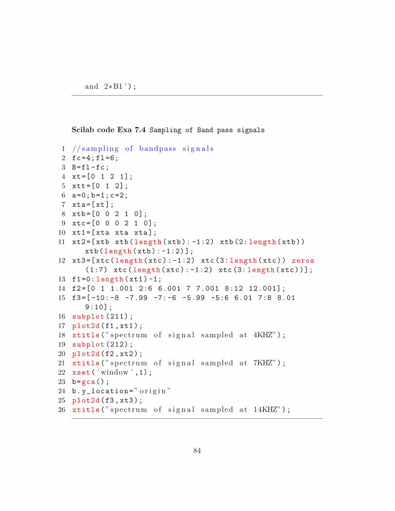
Scilab code Exa 7.4 Sampling of Band pass signals
1 // sampl ing o f bandpass s i g n a l s2 fc=4;fl=6;
3 B=fl -fc;
4 xt=[0 1 2 1];
5 xtt =[0 1 2];
6 a=0;b=1;c=2;
7 xta=[xt];
8 xtb =[0 0 2 1 0];
9 xtc =[0 0 0 2 1 0];
10 xt1=[xta xta xta];
11 xt2=[xtb xtb(length(xtb): -1:2) xtb(2: length(xtb))
xtb(length(xtb):-1:2)];
12 xt3=[xtc(length(xtc):-1:2) xtc (3: length(xtc)) zeros
(1:7) xtc(length(xtc):-1:2) xtc (3: length(xtc))];
13 f1=0: length(xt1) -1;
14 f2=[0 1 1.001 2:6 6.001 7 7.001 8:12 12.001];
15 f3=[-10:-8 -7.99 -7:-6 -5.99 -5:6 6.01 7:8 8.01
9:10];
16 subplot (211);
17 plot2d(f1,xt1);
18 xtitle(” spectrum o f s i g n a l sampled at 4KHZ”);19 subplot (212);
20 plot2d(f2,xt2);
21 xtitle(” spectrum o f s i g n a l sampled at 7KHZ”);22 xset( ’ window ’ ,1);23 b=gca();
24 b.y_location=” o r i g i n ”25 plot2d(f3,xt3);
26 xtitle(” spectrum o f s i g n a l sampled at 14KHZ”);
84
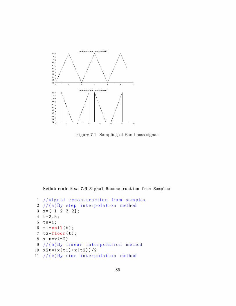
Figure 7.1: Sampling of Band pass signals
Scilab code Exa 7.6 Signal Reconstruction from Samples
1 // s i g n a l r e c o n s t r u c t i o n from sample s2 // ( a )By s t e p i n t e r p o l a t i o n method3 x=[-1 2 3 2];
4 t=2.5;
5 ts=1;
6 t1=ceil(t);
7 t2=floor(t);
8 x1t=x(t2)
9 // ( b )By l i n e a r i n t e r p o l a t i o n method10 x2t=(x(t1)+x(t2))/2
11 // ( c )By s i n c i n t e r p o l a t i o n method
85
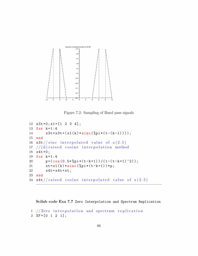
Figure 7.2: Sampling of Band pass signals
12 x3t =0;x1=[1 2 3 4];
13 for k=1:4
14 x3t=x3t+(x1(k)*sinc(%pi*(t-(k-1))));
15 end
16 x3t // s i n c i n t e r p o l a t e d v a l u e o f x ( 2 . 5 )17 // ( d ) r a i s e d c o s i n e i n t e r p o l a t i o n method18 x4t =0;
19 for k=1:4
20 p=(cos (0.5* %pi*(t-k+1))/(1-(t-k+1) ^2));
21 xt=x1(k)*sinc(%pi*(t-k+1))*p;
22 x4t=x4t+xt;
23 end
24 x4t // r a i s e d c o s i n e i n t e r p o l a t e d v a l u e o f x ( 2 . 5 )
Scilab code Exa 7.7 Zero Interpolation and Spectrum Replication
1 // Zero i n t e r p o l a t i o n and spectrum r e p l i c a t i o n2 XF=[0 1 2 1];
86
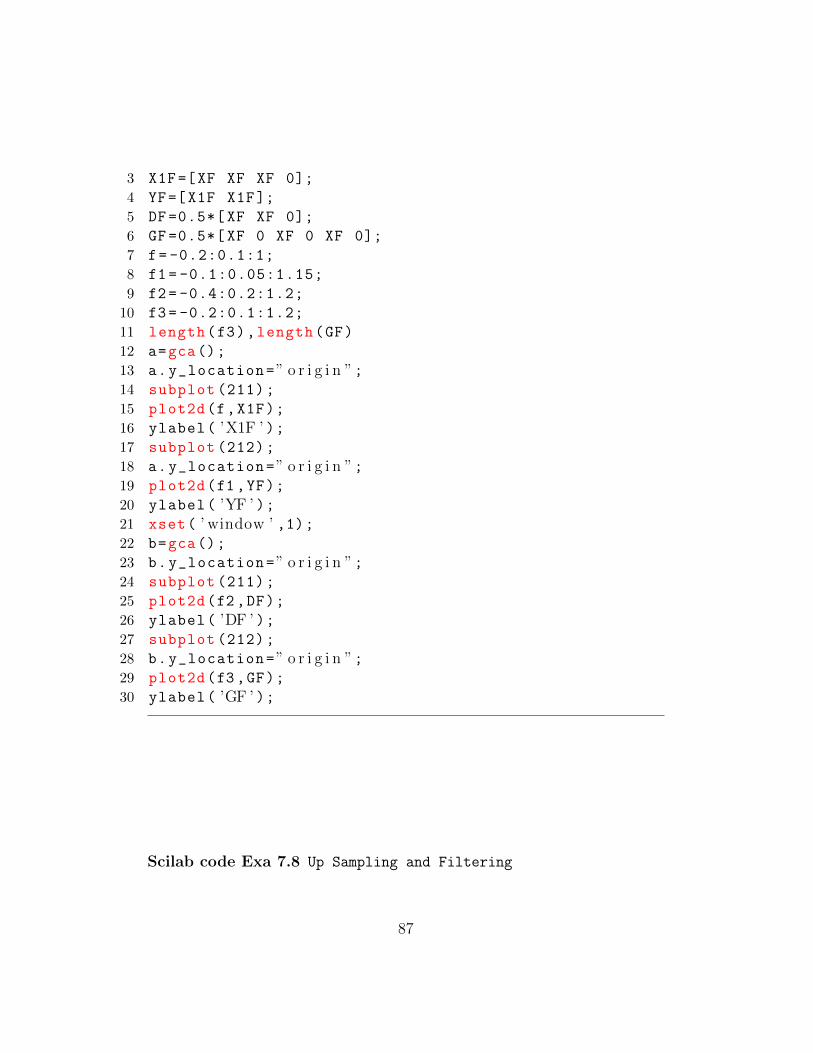
3 X1F=[XF XF XF 0];
4 YF=[X1F X1F];
5 DF =0.5*[ XF XF 0];
6 GF =0.5*[ XF 0 XF 0 XF 0];
7 f= -0.2:0.1:1;
8 f1 = -0.1:0.05:1.15;
9 f2 = -0.4:0.2:1.2;
10 f3 = -0.2:0.1:1.2;
11 length(f3),length(GF)
12 a=gca();
13 a.y_location=” o r i g i n ”;14 subplot (211);
15 plot2d(f,X1F);
16 ylabel( ’X1F ’ );17 subplot (212);
18 a.y_location=” o r i g i n ”;19 plot2d(f1,YF);
20 ylabel( ’YF ’ );21 xset( ’ window ’ ,1);22 b=gca();
23 b.y_location=” o r i g i n ”;24 subplot (211);
25 plot2d(f2,DF);
26 ylabel( ’DF ’ );27 subplot (212);
28 b.y_location=” o r i g i n ”;29 plot2d(f3,GF);
30 ylabel( ’GF ’ );
Scilab code Exa 7.8 Up Sampling and Filtering
87
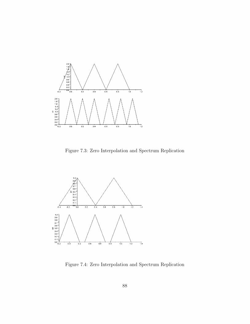
Figure 7.3: Zero Interpolation and Spectrum Replication
Figure 7.4: Zero Interpolation and Spectrum Replication
88
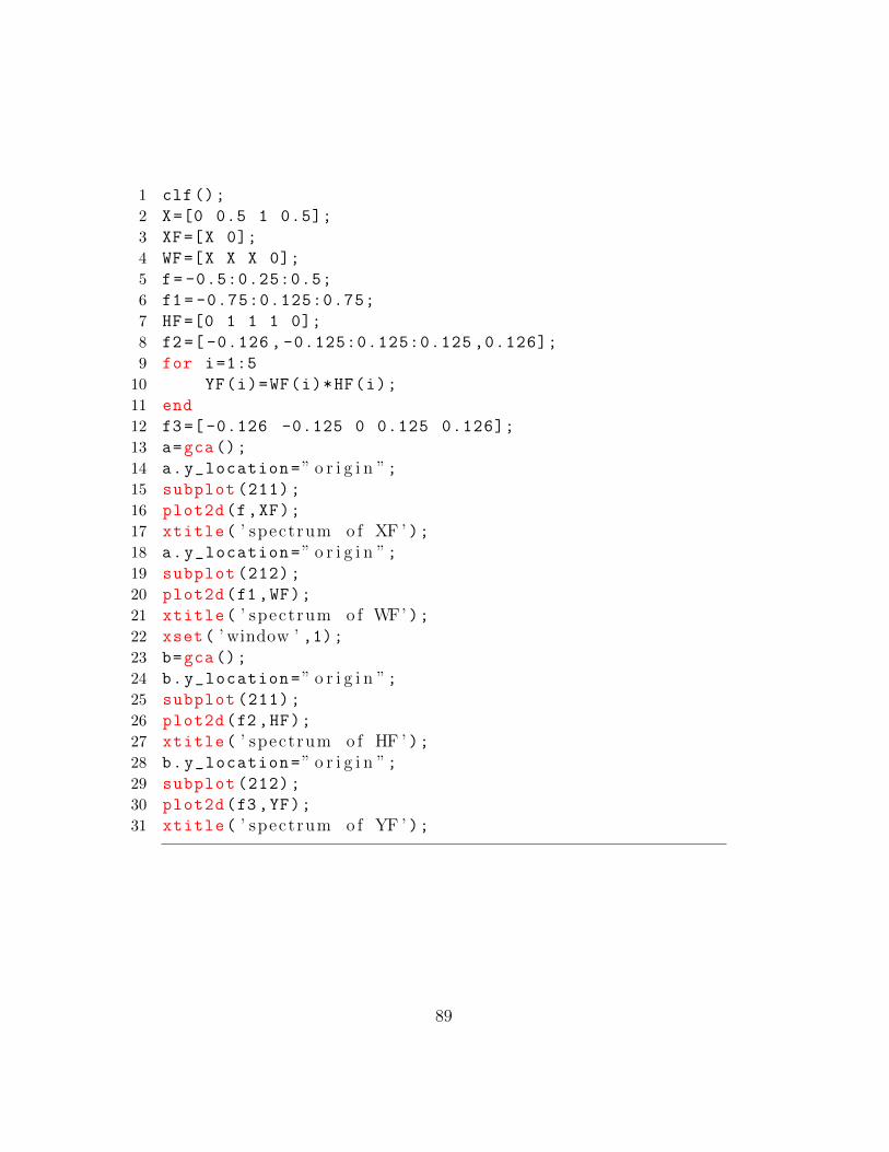
1 clf();
2 X=[0 0.5 1 0.5];
3 XF=[X 0];
4 WF=[X X X 0];
5 f= -0.5:0.25:0.5;
6 f1 = -0.75:0.125:0.75;
7 HF=[0 1 1 1 0];
8 f2 =[ -0.126 , -0.125:0.125:0.125 ,0.126];
9 for i=1:5
10 YF(i)=WF(i)*HF(i);
11 end
12 f3=[ -0.126 -0.125 0 0.125 0.126];
13 a=gca();
14 a.y_location=” o r i g i n ”;15 subplot (211);
16 plot2d(f,XF);
17 xtitle( ’ spectrum o f XF ’ );18 a.y_location=” o r i g i n ”;19 subplot (212);
20 plot2d(f1,WF);
21 xtitle( ’ spectrum o f WF’ );22 xset( ’ window ’ ,1);23 b=gca();
24 b.y_location=” o r i g i n ”;25 subplot (211);
26 plot2d(f2,HF);
27 xtitle( ’ spectrum o f HF ’ );28 b.y_location=” o r i g i n ”;29 subplot (212);
30 plot2d(f3,YF);
31 xtitle( ’ spectrum o f YF ’ );
89
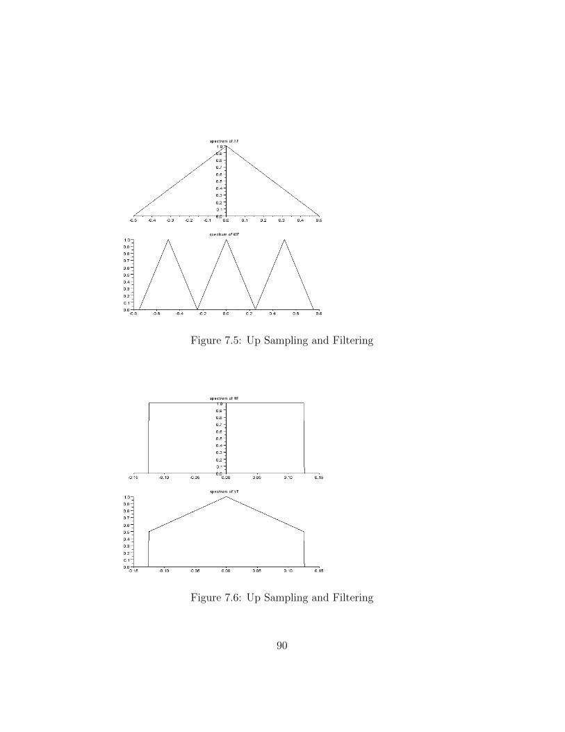
Figure 7.5: Up Sampling and Filtering
Figure 7.6: Up Sampling and Filtering
90
Scilab code Exa 7.9 Quantisation Effects
1 // ( a ) Q u a n t i s a t i o n e f f e c t s2 sig =0.005;
3 D=4;
4 B=log2(D/(sig*sqrt (12)));// no . o f sample s5 // v a l u e o f B to e n s u r e q u a n t i s a t i o n e r r o r to 5mv6 // ( b ) Q u a n t i s a t i o n e r r o r and n o i s e7 xn =0:0.2:2.0;
8 xqn =[0 0 0.5 0.5 1 1 1 1.5 1.5 2 2];
9 en=xn-xqn;// q u a n t i z a t i o n e r r o r10 // Q u a n t i s a t i o n s i g n a l top n o i s e r a t i o11 x=0;e=0;
12 for i=1: length(xn)
13 x=x+xn(i)^2;
14 e=e+en(i)^2;
15 end
16 // method 117 SNRQ =10* log10(x/e)
18 // method 219 SNRQ =10* log10(x/length(xn))+10.8+20* log10 (4) -20*
log10 (2)
20 SNRS =10* log10 (1.33) +10* log10 (12) +20* log10 (4) -20*
log10 (2)
21 // from r e s u l t s we s e e tha t SNRS i s s t a t i s t i c a le s t i m a t e
Scilab code Exa 7.10 ADC considerations
1 //ADC c o n s i d e r a t i o n s2 // ( a ) Aperture t ime TA3 B=12;
4 fo =15000; // band l i m i t e d f r q u e n c y5 TAm =(1/((2^B)))/(%pi*fo);
6 TAm=TAm *10^9
91
7 // Hence TA must s a t i s f y TA<=TAm nano s e c8 // ( b ) c o n v e r s i o n t ime o f q u a n t i z e r9 TA=4*10^ -9;
10 TH=10*10^ -6; // ho ld t ime11 S=30*10^3;
12 TCm =1/S-TA-TH;
13 TCm=TCm *10^6
14 // Hence TC must s a t i s f y TC<=TCm micro s e c15 // ( c ) Ho ld ing c a p a c i t a n c e C16 Vo=10;
17 TH=10*10^ -6;
18 B=12;
19 R=10^6; // input r e s i s t a n c e20 delv=Vo /(2^(B+1));
21 Cm=(Vo*TH)/(R*delv);
22 Cm=Cm *10^9
23 // Hence C must s a t i s f y C>=Cm nano f a r a d
Scilab code Exa 7.11 Anti Aliasing Filter Considerations
1 // Anti A l i a s i n g f i l t e r c o n s i d e r a t i o n s2 //minimum stop band a t t e n u a t i o n As3 B=input( ’ e n t e r no . o f b i t s ’ );// no . o f sample s4 n=input( ’ e n t e r band width i n KHZ ’ );5 As=20* log10 (2^B*sqrt (6))
6 // noma l i s ed f r e q u e n c y7 Vs =(10^(0.1* As) -1)^(1/(2*n))
8 fp=4; // pas s edge f r e q u e n c y9 fs=Vs*fp // s top band f r q u e n c y
10 S=2*fs // sampl ing f r e q u e n c y11 fa=S-fp // a l i a e d f r e q u e n c y12 Va=fa/fp;
13 // At t enua t i on at a l i a s e d f r e q u e n c y14 Aa=10* log10 (1+Va^(2*n))
92
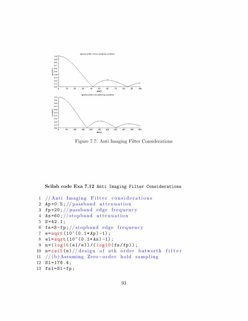
Figure 7.7: Anti Imaging Filter Considerations
Scilab code Exa 7.12 Anti Imaging Filter Considerations
1 // Anti Imaging F i l t e r c o n s i d e r a t i o n s2 Ap=0.5; // passband a t t e n u a t i o n3 fp=20; // passband edge f r e q u e n c y4 As=60; // stopband a t t e n u a t i o n5 S=42.1;
6 fs=S-fp;// stopband edge f r e q u e n c y7 e=sqrt (10^(0.1* Ap) -1);
8 e1=sqrt (10^(0.1* As) -1);
9 n=(log10(e1/e))/( log10(fs/fp));
10 n=ceil(n)// d e s i g n o f nth o r d e r butworth f i l t e r11 // ( b ) Assuming Zero−o r d e r ho ld sampl ing12 S1 =176.4;
13 fs1=S1 -fp;
93
14 Ap =0.316;
15 e2=sqrt (10^(0.1* Ap) -1);
16 n1=( log10(e1/e2))/(log(fs1/fp));//new o r d e r o fbutworth f i l t e r
17 n1=ceil(n1)
18 f=0:100;
19 x=abs(sinc(f*%pi/S));
20 f1 =0:500;
21 x1=abs(sinc(f1*%pi/S1));
22 a=gca();
23 subplot (211);
24 plot2d(f,x);
25 xtitle(” s p e c t r a under normal sampl ing c o n d i t i o n ”,” f (kHZ) ”,” s i n c ( f / s1 ) ”);
26 subplot (212);
27 plot2d(f1,x1);
28 xtitle(” s p e c t r a under ove r sampl ing c o n d i t i o n ”,” f (kHZ) ”,” s i n c ( f / s1 ) ”);
94
Chapter 8
The Discrete Fourier Transformand its Applications
Scilab code Exa 8.1 DFT from Defining Relation
1 //DFT from d e f i n i n g r e l a t i o n2 //N−p o i n t DFT3 x=[1 2 1 0];
4 XDFT=fft(x,-1);
5 disp(XDFT , ’ The DFT o f x [ n ] i s ’ );6 //DFT o f p e r i o d i c s i g n a l x with p e r i o d N=4
Scilab code Exa 8.2 The DFT and conjugate Symmetry
1 //The DTFT and c o n j u g a t e symmetry2 //8−p o i n t DFT3 x=[1 1 0 0 0 0 0 0];
4 XDFT=fft(x,-1);
5 disp(XDFT , ’ The DFT o f x i s ’ );6 disp( ’ from c o n j u g a t e symmetry we s e e XDFT[ k ]=XDFT[8−
k ] ’ );
95
Scilab code Exa 8.3 Circular Shift and Flipping
1 // C i r c u l a r s h i f t and f l i p p i n g2 // ( a ) r i g h t c i r c u l a r s h i f t3 y=[1 2 3 4 5 0 0 6];
4 f=y;g=y;h=y;
5 for i=1:2
6 b=f(length(f));
7 for j=length(f):-1:2
8 f(j)=f(j-1);
9 end
10 f(1)=b;
11 end
12 disp(f, ’By r i g h t c i r c u l a r s h i f t y [ n−2] i s ’ );13 // ( b ) l e f t c i r c u l a r s h i f t14 for i=1:2
15 a=g(1);
16 for j=1: length(g) -1
17 g(j)=g(j+1);
18 end
19 g(length(g))=a;
20 end
21 disp(g, ’By l e f t c i r c u l a r s h i f t y [ n+2] i s ’ );22 // ( c ) f l i p p i n g p r o p e r t y23 h=[h(1) h(length(h):-1:2)];
24 disp(h, ’By f l i p p i n g p r o p e r t y y[−n ] i s ’ );
Scilab code Exa 8.4 Properties of DFT
1 x=[1 2 1 0];
2 XDFT=fft(x,-1)
3 // ( a ) t ime s h i f t p r o p e r t y
96
4 y=x;
5 for i=1:2
6 a=y(1);
7 for j=1: length(y) -1
8 y(j)=y(j+1);
9 end
10 y(length(y))=a;
11 end
12 YDFT=fft(y,-1)
13 disp(YDFT , ’By Time−S h i f t p r o p e r t y DFT o f x [ n−2] i s ’ );
14 // ( b ) f l i p p i n g p r o p e r t y15 g=[x(1) x(length(x): -1:2)]
16 GDFT=fft(g,-1)
17 disp(GDFT , ’By Time r e v e r s a l p r o p e r t y DFT o f x[−n ] i s’ );
18 // ( c ) c o n j u g a t i o n p r o p e r t y19 p=XDFT;
20 PDFT=[p(1) p(4: -1:2)];
21 disp(YDFT , ’BY c o n j u g a t i o n p r o p e r t y DFT o f x ∗ [ n ] i s ’ );
Scilab code Exa 8.5a Properties of DFT
1 // p r o p e r t i e s o f DFT2 // a1 ) product3 xn=[1 2 1 0];
4 XDFT=fft(xn ,-1)
5 hn=xn.*xn
6 HDFT=fft(hn ,-1)
7 HDFT1 =1/4*( convol(XDFT ,XDFT))
8 HDFT1=[HDFT1 ,zeros (8:12) ];
9 HDFT2=[HDFT1 (1:4);HDFT1 (5:8);HDFT1 (9:12) ];
10 HDFT3 =[0 0 0 0];
11 for i=1:4
97
12 for j=1:3
13 HDFT3(i)=HDFT3(i)+HDFT2(j,i);
14 end
15 end
16 disp(HDFT3 , ’DFT o f x [ n ] ˆ 2 i s ’ );17 // a2 ) p e r i o d i c c o n v o l u t i o n18 vn=convol(xn ,xn);
19 vn=[vn,zeros (8:12) ];
20 vn=[vn (1:4);vn (5:8);vn (9:12) ];
21 vn1 =[0 0 0 0];
22 for i=1:4
23 for j=1:3
24 vn1(i)=vn1(i)+vn(j,i);
25 end
26 end
27 VDFT=fft(vn1 ,-1);
28 VDFT1=XDFT.*XDFT;
29 disp(VDFT1 , ’DFT o f x [ n ] ∗ x [ n ] i s ’ );30 // a3 ) s i g n a l ene rgy ( p a r c e w e l l ’ s theorem )31 xn2=xn.^2;
32 E=0;
33 for i=1: length(xn2)
34 E=E+abs(xn2(i));
35 end
36 XDFT2=XDFT .^2
37 E1=0;
38 for i=1: length(XDFT2)
39 E1=E1+abs(XDFT2(i));
40 end
41 E ,(1/4)*E1;
42 disp (1/4*E1, ’ The ene rgy o f the s i g n a l i s ’ );
Scilab code Exa 8.5b Properties of DFT
1 // b1 ) modulat ion
98
2 XDFT =[4 -2*%i 0 2*%i];
3 xn=dft(XDFT ,1)
4 for i=1: length(xn)
5 zn(i)=xn(i)*%e^((%i*%pi*(i-1))/2);
6 end
7 disp(zn, ’ The IDFT o f XDFT[ k−1] i s ’ );8 ZDFT =[2*%i 4 -2*%i 0];
9 zn1=dft(ZDFT ,1)
10 // b2 ) p e r i o d i c c o n v o l u t i o n11 HDFT=( convol(XDFT ,XDFT))
12 HDFT=[HDFT ,zeros (8:12) ];
13 HDFT=[HDFT (1:4);HDFT (5:8);HDFT (9:12) ];
14 HDFT1 =[0 0 0 0];
15 for i=1:4
16 for j=1:3
17 HDFT1(i)=HDFT1(i)+HDFT(j,i);
18 end
19 end
20 HDFT1;
21 hn=dft(HDFT1 ,1)
22 hn1 =4*(xn.*xn);
23 disp(hn1 , ’ The IDFT o f XDFT∗XDFT i s ’ );24 // b3 ) product25 WDFT=XDFT.*XDFT;
26 wn=dft(WDFT ,1)
27 wn1=convol(xn,xn);
28 wn1=[wn1 ,zeros (8:12) ];
29 wn1=[wn1 (1:4);wn1 (5:8);wn1 (9:12) ];
30 WN=[0 0 0 0];
31 for i=1:4
32 for j=1:3
33 WN(i)=WN(i)+wn1(j,i);
34 end
35 end
36 disp(WN, ’ The IDFT o f XDFT.XDFT i s ’ );37 // b4 ) C e n t r a l o r d i n a t e s and s i g n a l Energy38 E=0;
39 for i=1: length(xn)
99
40 E=E+abs(xn(i)^2);
41 end
42 disp(E, ’ the s i g n a l ene rgy i s ’ );
Scilab code Exa 8.5c Properties of DFT
1 // Regu lar c o n v o l u t i o n2 xn=[1 2 1 0];
3 yn=[1 2 1 0 0 0 0];
4 YDFT=fft(yn ,-1)
5 SDFT=YDFT.*YDFT
6 sn=fft(SDFT ,1)
7 sn1=convol(xn,xn)
Scilab code Exa 8.6 Signal and Spectrum Replication
1 // S i g n a l and spectrum r e p l i c a t i o n2 xn=[2 3 2 1];
3 XDFT=fft(xn ,-1)
4 yn=[xn xn xn];
5 YDFT=fft(yn ,-1)
6 YDFT1 =3*[ XDFT (1:1/3: length(XDFT))];
7 for i=2:3
8 YDFT1(i:3: length(YDFT1))=0;
9 end
10 YDFT1 (12: -1:11) =0;
11 disp(YDFT1 , ’ the DFT o f x [ n / 3 ] i s ’ );12 hn=[xn (1:1/3: length(xn))]
13 for i=2:3
14 hn(i:3: length(hn))=0;
15 end
16 hn(12: -1:11) =0;
17 hn
100
18 HDFT=fft(hn ,-1)
19 HDFT1=[XDFT;XDFT;XDFT];
20 disp(HDFT1 , ’ the DFT o f y [ n ] = [ x [ n ] , x [ n ] , x [ n ] ] i s ’ );
Scilab code Exa 8.7 Relating DFT and DTFT
1 // r e l a t i n g DFT and IDFT2 XDFT1 =[4 -2*%i 0 2*%i];
3 xn1=fft(XDFT1 ,1);
4 disp(xn1 , ’ The IDFT o f XDFT1 ’ );5 XDFT2 =[12 -24*%i 0 4*%e^(%i*%pi/4) 0 4*%e^(-%i*%pi
/4) 0 24*%i];
6 xn2=fft(XDFT2 ,1);
7 disp(xn2 , ’ The IDFT o f XDFT1 ’ );
Scilab code Exa 8.8 Relating DFT and DTFT
1 // R e l a t i n g DFT and DTFT2 xn=[1 2 1 0];
3 XDFT=fft(xn ,-1);
4 // f o r F=k /4 , k =0 ,1 ,2 ,35 for k=1:4
6 XF(k)=1+2*%e^(-%i*%pi*(k-1)/2)+%e^(-%i*%pi*(k-1)
);
7 end
8 XF ,XDFT
9 disp(XF, ’ The DFT o f x [ n ] i s ’ );
Scilab code Exa 8.9a The DFT and DFS of sinusoids
101
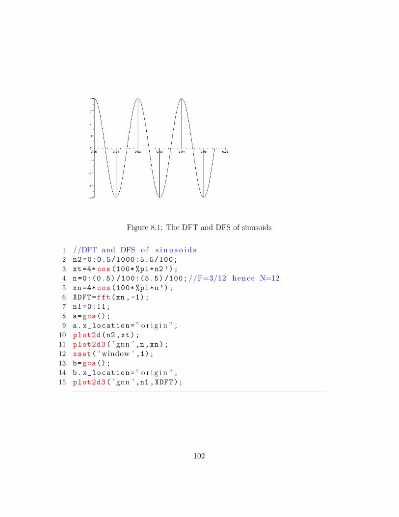
Figure 8.1: The DFT and DFS of sinusoids
1 //DFT and DFS o f s i n u s o i d s2 n2 =0:0.5/1000:5.5/100;
3 xt=4*cos (100* %pi*n2 ’);
4 n=0:(0.5) /100:(5.5) /100; //F=3/12 hence N=125 xn=4*cos (100* %pi*n’);
6 XDFT=fft(xn ,-1);
7 n1 =0:11;
8 a=gca();
9 a.x_location=” o r i g i n ”;10 plot2d(n2,xt);
11 plot2d3( ’ gnn ’ ,n,xn);12 xset( ’ window ’ ,1);13 b=gca();
14 b.x_location=” o r i g i n ”;15 plot2d3( ’ gnn ’ ,n1 ,XDFT);
102
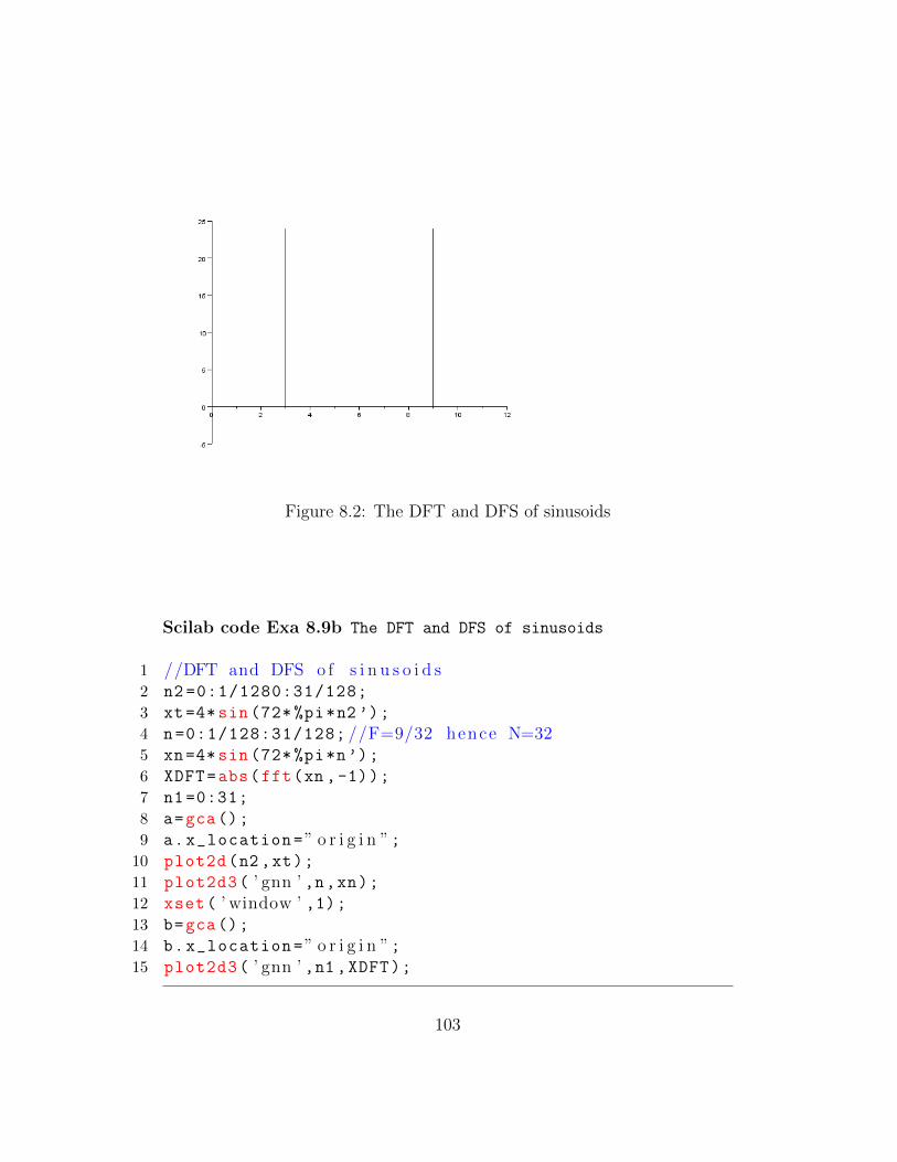
Figure 8.2: The DFT and DFS of sinusoids
Scilab code Exa 8.9b The DFT and DFS of sinusoids
1 //DFT and DFS o f s i n u s o i d s2 n2 =0:1/1280:31/128;
3 xt=4*sin (72* %pi*n2 ’);
4 n=0:1/128:31/128; //F=9/32 hence N=325 xn=4*sin (72* %pi*n’);
6 XDFT=abs(fft(xn ,-1));
7 n1 =0:31;
8 a=gca();
9 a.x_location=” o r i g i n ”;10 plot2d(n2,xt);
11 plot2d3( ’ gnn ’ ,n,xn);12 xset( ’ window ’ ,1);13 b=gca();
14 b.x_location=” o r i g i n ”;15 plot2d3( ’ gnn ’ ,n1 ,XDFT);
103
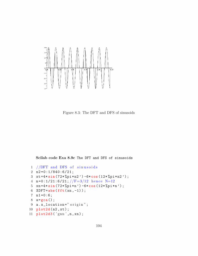
Figure 8.3: The DFT and DFS of sinusoids
Scilab code Exa 8.9c The DFT and DFS of sinusoids
1 //DFT and DFS o f s i n u s o i d s2 n2 =0:1/840:6/21;
3 xt=4*sin (72* %pi*n2 ’) -6*cos (12* %pi*n2 ’);
4 n=0:1/21:6/21; //F=3/12 hence N=125 xn=4*sin (72* %pi*n’) -6*cos (12* %pi*n’);
6 XDFT=abs(fft(xn ,-1));
7 n1=0:6;
8 a=gca();
9 a.x_location=” o r i g i n ”;10 plot2d(n2,xt);
11 plot2d3( ’ gnn ’ ,n,xn);
104
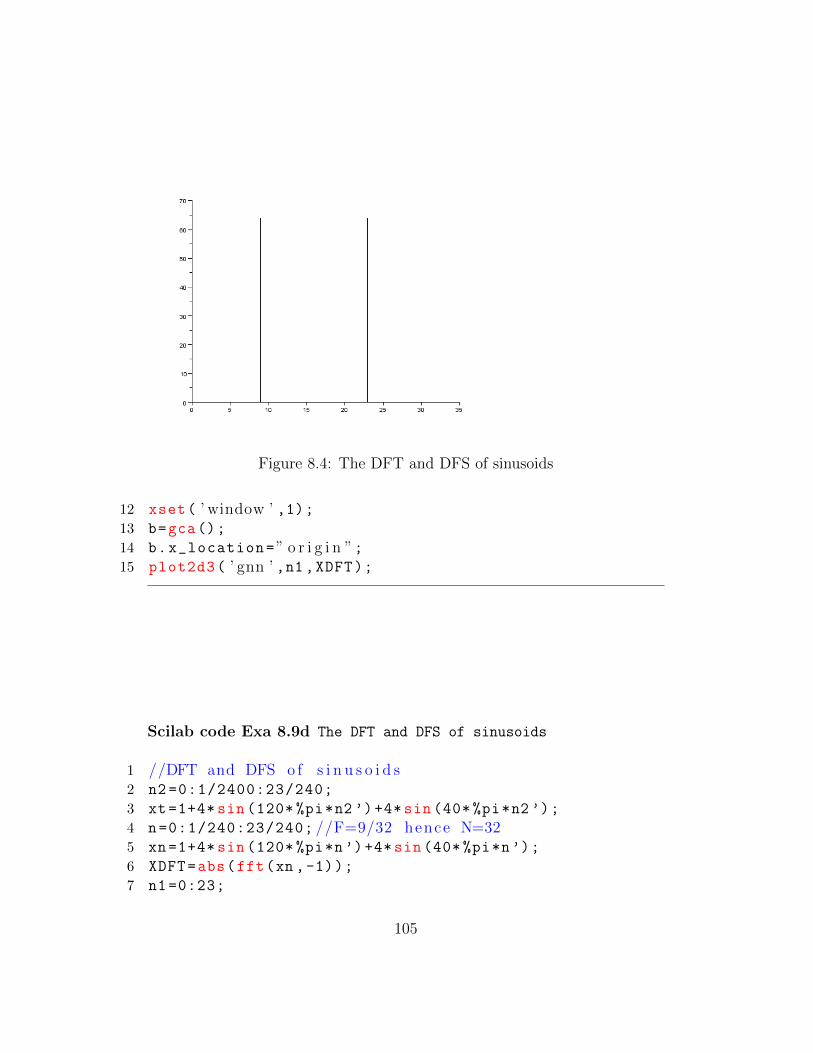
Figure 8.4: The DFT and DFS of sinusoids
12 xset( ’ window ’ ,1);13 b=gca();
14 b.x_location=” o r i g i n ”;15 plot2d3( ’ gnn ’ ,n1 ,XDFT);
Scilab code Exa 8.9d The DFT and DFS of sinusoids
1 //DFT and DFS o f s i n u s o i d s2 n2 =0:1/2400:23/240;
3 xt=1+4* sin (120* %pi*n2 ’)+4*sin (40* %pi*n2 ’);
4 n=0:1/240:23/240; //F=9/32 hence N=325 xn=1+4* sin (120* %pi*n’)+4*sin (40* %pi*n’);
6 XDFT=abs(fft(xn ,-1));
7 n1 =0:23;
105
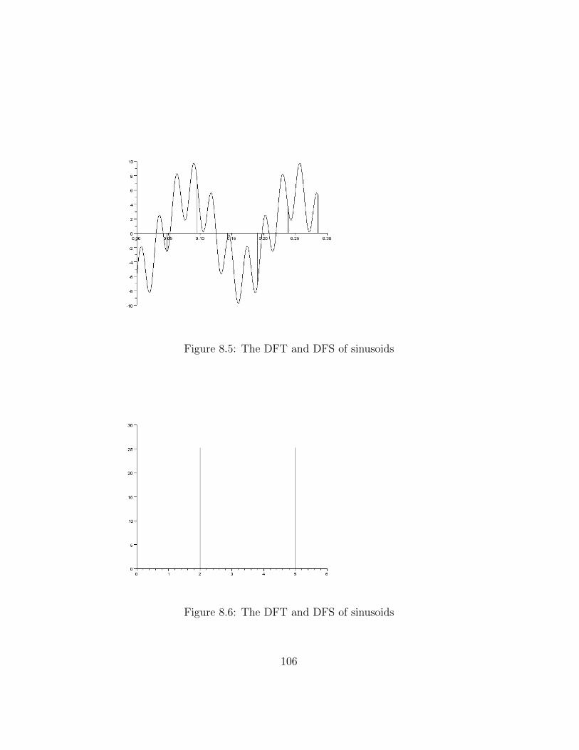
Figure 8.5: The DFT and DFS of sinusoids
Figure 8.6: The DFT and DFS of sinusoids
106
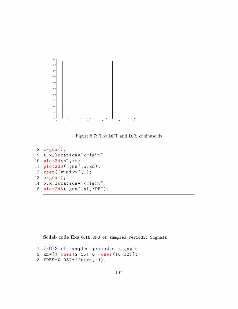
Figure 8.7: The DFT and DFS of sinusoids
8 a=gca();
9 a.x_location=” o r i g i n ”;10 plot2d(n2,xt);
11 plot2d3( ’ gnn ’ ,n,xn);12 xset( ’ window ’ ,1);13 b=gca();
14 b.x_location=” o r i g i n ”;15 plot2d3( ’ gnn ’ ,n1 ,XDFT);
Scilab code Exa 8.10 DFS of sampled Periodic Signals
1 //DFS o f sampled p e r i o d i c s i g n a l s2 xn=[0 ones (2:16) 0 -ones (18:32) ];
3 XDFS =0.032* fft(xn ,-1);
107
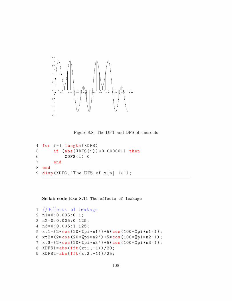
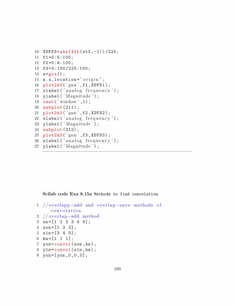
Figure 8.8: The DFT and DFS of sinusoids
4 for i=1: length(XDFS)
5 if (abs(XDFS(i)) <0.000001) then
6 XDFS(i)=0;
7 end
8 end
9 disp(XDFS , ’ The DFS o f x [ n ] i s ’ );
Scilab code Exa 8.11 The effects of leakage
1 // E f f e c t s o f l e a k a g e2 n1 =0:0.005:0.1;
3 n2 =0:0.005:0.125;
4 n3 =0:0.005:1.125;
5 xt1 =(2* cos (20* %pi*n1 ’)+5* cos (100* %pi*n1 ’));
6 xt2 =(2* cos (20* %pi*n2 ’)+5* cos (100* %pi*n2 ’));
7 xt3 =(2* cos (20* %pi*n3 ’)+5* cos (100* %pi*n3 ’));
8 XDFS1=abs(fft(xt1 ,-1))/20;
9 XDFS2=abs(fft(xt2 ,-1))/25;
108
10 XDFS3=abs(fft(xt3 ,-1))/225;
11 f1 =0:5:100;
12 f2 =0:4:100;
13 f3 =0:100/225:100;
14 a=gca();
15 a.x_location=” o r i g i n ”;16 plot2d3( ’ gnn ’ ,f1 ,XDFS1);17 xlabel( ’ ana l og f r e q u e n c y ’ );18 ylabel( ’ Magnitude ’ );19 xset( ’ window ’ ,1);20 subplot (211);
21 plot2d3( ’ gnn ’ ,f2 ,XDFS2);22 xlabel( ’ ana l og f r e q u e n c y ’ );23 ylabel( ’ Magnitude ’ );24 subplot (212);
25 plot2d3( ’ gnn ’ ,f3 ,XDFS3);26 xlabel( ’ ana l og f r e q u e n c y ’ );27 ylabel( ’ Magnitude ’ );
Scilab code Exa 8.15a Methods to find convolution
1 // over l app−add and ove r l ap−save methods o fc o n v o l u t i o n
2 // ove r l ap−add method3 xn=[1 2 3 3 4 5];
4 xon =[1 2 3];
5 x1n =[3 4 5];
6 hn=[1 1 1];
7 yon=convol(xon ,hn);
8 y1n=convol(x1n ,hn);
9 yon=[yon ,0,0,0];
109
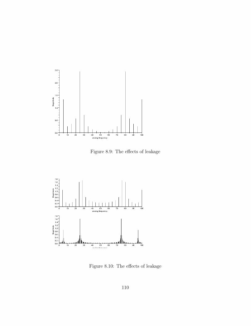
Figure 8.9: The effects of leakage
Figure 8.10: The effects of leakage
110
10 y1n=[0,0,0,y1n];
11 yn=yon+y1n
12 yn1=convol(xn,hn)
Scilab code Exa 8.15b Methods to find convolution
1 // ( b ) ove r l ap−save method2 xn=[1 2 3 3 4 5];
3 hn=[1 1 1];
4 xon =[0 0 1 2 3];
5 x1n =[2 3 3 4 5];
6 x2n =[4 5 0 0 0];
7 yon=convol(xon ,hn);
8 y1n=convol(x1n ,hn);
9 y2n=convol(x2n ,hn);
10 yno=yon (3:5);
11 yn1=y1n (3:5);
12 yn2=y2n (3:5);
13 yn=[yno yn1 yn2]
14 YN=convol(xn ,hn)
Scilab code Exa 8.16 Signal Interpolation using FFT
1 // s i g n a l i n t e r p o l a t i o n u s i n g FFT2 xn=[0 1 0 -1];
3 XDFT=fft(xn ,-1)
4 ZT=[0 -2*%i 0 zeros (1:27) 0 2*%i];
5 xn1=fft(ZT ,1);
6 t=0:1/ length(xn1):1 -(1/ length(xn1));
7 a=gca();
8 a.x_location=” o r i g i n ”;
111
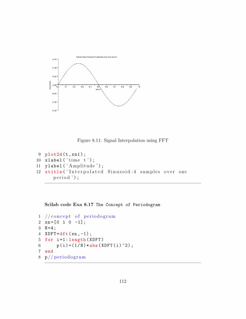
Figure 8.11: Signal Interpolation using FFT
9 plot2d(t,xn1);
10 xlabel( ’ t ime t ’ );11 ylabel( ’ Amplitude ’ );12 xtitle( ’ I n t e r p o l a t e d S i n u s o i d : 4 sample s ove r one
p e r i o d ’ );
Scilab code Exa 8.17 The Concept of Periodogram
1 // concep t o f per iodogram2 xn=[0 1 0 -1];
3 N=4;
4 XDFT=dft(xn ,-1);
5 for i=1: length(XDFT)
6 p(i)=(1/N)*abs(XDFT(i)^2);
7 end
8 p// per iodogram
112
Scilab code Exa 8.18 DFT from matrix formulation
1 //The DFT from the matr ix f o r m u l a t i o n2 xn =[1;2;1;0];
3 w=exp(-%i*%pi /2);
4 for i=1:4
5 for j=1:4
6 WN(i,j)=w^((i-1)*(j-1));
7 end
8 end
9 XDFT=WN*xn
Scilab code Exa 8.19 Using DFT to find IDFT
1 // u s i n g DFT to f i n d IDFT2 XDFT =[4; -2*%i;0;2* %i];
3 XDFTc =[4;2* %i;0;-2*%i];
4 w=exp(-%i*%pi /2);
5 for i=1:4
6 for j=1:4
7 WN(i,j)=w^((i-1)*(j-1));
8 end
9 end
10 xn =1/4*( WN*XDFTc)
Scilab code Exa 8.20 Decimation in Frequency FFT algorithm
1 //A f o u r p o i n t dec imat ion−in−f r e q u e n c y FFT a l g o r i t h m2 x=[1 2 1 0];
113
3 w=-%i;
4 xdft (1)=x(1)+x(3)+x(2)+x(4);
5 xdft (2)=x(1)-x(3)+w*(x(2)-x(4));
6 xdft (3)=x(1)+x(3)-x(2)-x(4);
7 xdft (4)=x(1)-x(3)-w*(x(2)-x(4));
8 XDFT=dft(x,-1);
9 xdft ,XDFT
Scilab code Exa 8.21 Decimation in time FFT algorithm
1 //A f o u r p o i n t dec imat ion−in−t ime FFT a l g o r i t h m2 x=[1 2 1 0];
3 w=-%i;
4 xdft =[0 0 0 0];
5 for i=1:4
6 for j=1:4
7 xdft(i)=xdft(i)+x(j)*w^((i-1)*(j-1));
8 end
9 end
10 XDFT=dft(x,-1);
11 xdft ,XDFT
Scilab code Exa 8.22 4 point DFT from 3 point sequence
1 //A 4−p o i n t DFT from a 3−p o i n t s equence2 xn =[1;2;1];
3 w=exp(-%i*%pi/2);
4 for i=1:4
5 for j=1:3
6 WN(i,j)=w^((i-1)*(j-1));
7 end
8 end
9 XDFT=WN*xn
114
Scilab code Exa 8.23 3 point IDFT from 4 point DFT
1 //A 3−p o i n t IDFT from 4−p o i n t DFT2 XDFT =[4; -2*%i;0;2* %i];
3 w=exp(-%i*%pi/2);
4 for i=1:4
5 for j=1:3
6 WN(i,j)=w^((i-1)*(j-1));
7 end
8 end
9 WI=WN ’;
10 xn =1/4*( WI*XDFT)
Scilab code Exa 8.24 The importance of Periodic Extension
1 //The impor tance o f P e r i o d i c e x t e n s i o n2 // ( a ) For M=33 x=[1 2 1];
4 XDFT=fft(x,-1)’
5 w=exp(-%i*2* %pi/3);
6 for i=1:3
7 for j=1:3
8 WN(i,j)=w^((i-1)*(j-1));
9 end
10 end
11 WI=WN ’;
12 xn=1/3*WI*XDFT
13 //The r e s u l t i s p e r i o d i c with M=3 & ; 1 p e r i o de q u a l s x [ n ]
14 // ( b ) For M=415 y=[1 2 1 0];
115
16 YDFT=fft(y,-1)’
17 w=exp(-%i*%pi/2);
18 for i=1:4
19 for j=1:4
20 WN(i,j)=w^((i-1)*(j-1));
21 end
22 end
23 WI=WN ’;
24 yn=1/4*WI*YDFT
116
Chapter 9
Design of IIR Filters
Scilab code Exa 9.1 Response Invariant Mappings
1 // Response i n v a r i a n t mappings2 s=%s;z=%z;
3 HS=1/(s+1);
4 f=0:0.05:0.5;
5 HS1=horner(HS ,(%i*%pi*2*f’));
6 ts=1;
7 HZ=z/(z -0.3679);
8 HZ1=horner(HZ,exp(%i*%pi *2*f’));
9 a=gca();
10 a.x_location=” o r i g i n ”;11 subplot (211)
12 plot2d(f,HS1);
13 plot2d(f,HZ1);
14 xlabel( ’ Analog f r e q u e n c y f ( Hz ) ’ );15 ylabel( ’ Magnitude ’ );16 xtitle( ’ magnitude o f H( s ) and H( z ) ’ );17 HZ1=HZ1 -0.582; // magnitude a f t e r ga in matching at dc18 b=gca();
19 b.x_location=” o r i g i n ”;20 subplot (212);
21 plot2d(f,HS1);
117
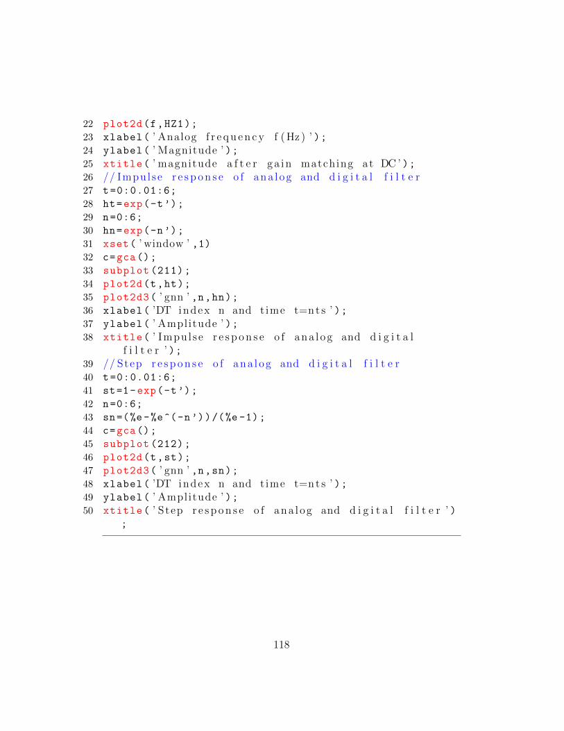
22 plot2d(f,HZ1);
23 xlabel( ’ Analog f r e q u e n c y f ( Hz ) ’ );24 ylabel( ’ Magnitude ’ );25 xtitle( ’ magnitude a f t e r ga in matching at DC ’ );26 // Impul se r e s p o n s e o f ana l og and d i g i t a l f i l t e r27 t=0:0.01:6;
28 ht=exp(-t’);
29 n=0:6;
30 hn=exp(-n’);
31 xset( ’ window ’ ,1)32 c=gca();
33 subplot (211);
34 plot2d(t,ht);
35 plot2d3( ’ gnn ’ ,n,hn);36 xlabel( ’DT index n and t ime t=nt s ’ );37 ylabel( ’ Amplitude ’ );38 xtitle( ’ Impul se r e s p o n s e o f ana l og and d i g i t a l
f i l t e r ’ );39 // Step r e s p o n s e o f ana l og and d i g i t a l f i l t e r40 t=0:0.01:6;
41 st=1-exp(-t’);
42 n=0:6;
43 sn=(%e-%e^(-n’))/(%e -1);
44 c=gca();
45 subplot (212);
46 plot2d(t,st);
47 plot2d3( ’ gnn ’ ,n,sn);48 xlabel( ’DT index n and t ime t=nt s ’ );49 ylabel( ’ Amplitude ’ );50 xtitle( ’ Step r e s p o n s e o f ana l og and d i g i t a l f i l t e r ’ )
;
118
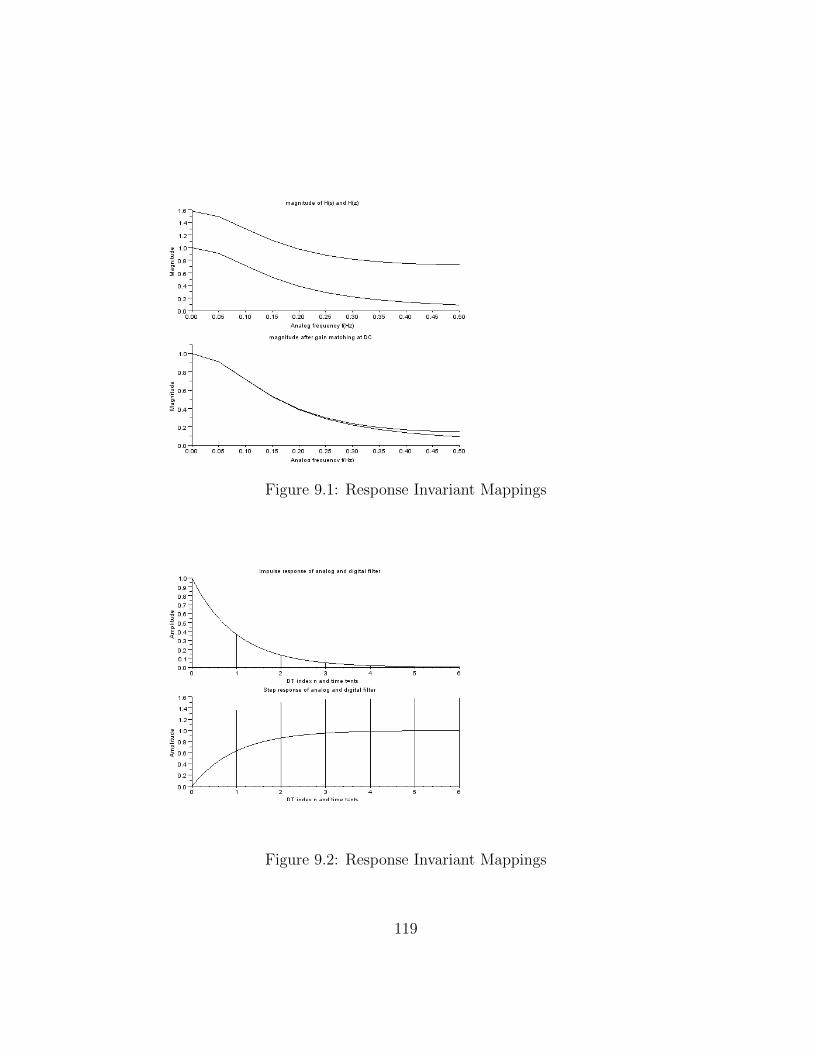
Figure 9.1: Response Invariant Mappings
Figure 9.2: Response Invariant Mappings
119

Scilab code Exa 9.2 Impulse Invariant Mappings
1 // Impul se i n v a r i a n t mappings2 // ( a ) c o n v e r t i n g H( s )=4s +7/ s ˆ2+5 s+4 to H( z ) u s i n g
impu l s e i n v a r i a n c e3 s=%s;
4 z=%z;
5 HS=(4*s+7)/(s^2+5*s+4);
6 pfss(HS)
7 ts=0.5;
8 HZ=3*z/(z-%e^(-4*ts))+z/(z-%e^(-ts))
9 // ( b ) c o n v e r t i n g H( s )=4s +7/ s ˆ2+5 s+4 to H( z ) u s i n gimpu l s e i n v a r i a n c e
10 HS1 =4/((s+1)*(s^2+4*s+5))
11 pfss(HS1);
12 HZ1 =2*z/(z-%e^-ts)+(2*1.414*z^2*cos ( -0.75* %pi)
-2*1.414*(z/%e)*cos (0.5 -0.75* %pi))/(z^2 -2*(z/%e)*
cos (0.5)+%e^-2)
Scilab code Exa 9.3ab Modified Impulse Invariant Design
1 // ( a ) Impul se i n v a r i a n t d e s i g n2 s=%s;z=%z;
3 HS=1/(s+1);
4 H1s=horner(HS ,3*s/%pi)
5 H1z=%pi/3*z/(z-%e^(-%pi /3))
6 // Mod i f i ed inmpul se i n v a r i a n t d e s i g n7 HZ=z/(z-1/%e);
8 HMZ =0.5*(z+1/%e)/(z-1/%e);// m o d i f i e d t r a n s f e rf u n c t i o n
9 H1Z=HZ/horner(HZ ,1)
10 HM1Z=HMZ/horner(HMZ ,1)
11 f=0:0.05:0.5;
120
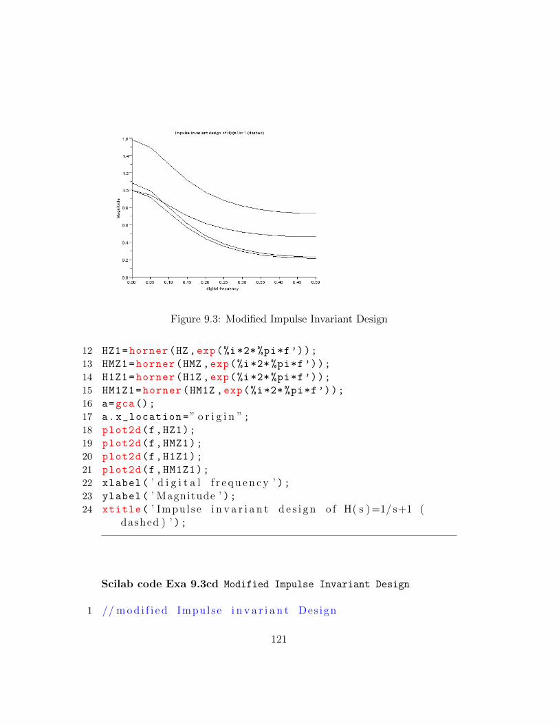
Figure 9.3: Modified Impulse Invariant Design
12 HZ1=horner(HZ,exp(%i*2* %pi*f’));
13 HMZ1=horner(HMZ ,exp(%i*2*%pi*f’));
14 H1Z1=horner(H1Z ,exp(%i*2*%pi*f’));
15 HM1Z1=horner(HM1Z ,exp(%i*2* %pi*f’));
16 a=gca();
17 a.x_location=” o r i g i n ”;18 plot2d(f,HZ1);
19 plot2d(f,HMZ1);
20 plot2d(f,H1Z1);
21 plot2d(f,HM1Z1);
22 xlabel( ’ d i g i t a l f r e q u e n c y ’ );23 ylabel( ’ Magnitude ’ );24 xtitle( ’ Impul se i n v a r i a n t d e s i g n o f H( s ) =1/ s+1 (
dashed ) ’ );
Scilab code Exa 9.3cd Modified Impulse Invariant Design
1 // m o d i f i e d Impul se i n v a r i a n t Des ign
121
2 // ( c )H( s )=4s +7/ s ˆ2+5 s+43 s=%s;z=%z;
4 HS=(4*s+7)/(s^2+5*s+4);
5 [d1]= degree(numer(HS));
6 [d2]= degree(denom(HS));
7 HZ=((3*z)/(z-%e^-2))+(z/(z-%e^-0.5))
8 if (d2 -d1==1) then
9 h=(4+7/ %inf)/(1+5/ %inf +4/ %inf)
10 HMZ=HZ -0.5*h
11 else
12 HMZ=HZ
13 end
14 HS1 =4/((s+1)*(s^2+4*s+5))
15 HZ1 =(0.2146*z^2+0.093*z)/(z^3 -1.2522*z^2+0.527*z
-0.0821);
16 [d1]= degree(numer(HS1));
17 [d2]= degree(denom(HS1));
18 if (d2 -d1==1) then
19 HMZ1=HZ1 -0.5*h
20 else
21 HMZ1=HZ1
22 end
Scilab code Exa 9.5 Mappings from Difference Algorithms
1 // Mappings from d i f f e r e n c e a l g o r i t h m s2 // Backward d i f f e r e n c e mappings3 s=%s;z=%z;
4 ts=1;a=1;
5 HS=1/(s+a);
6 HZa=horner(HS ,(z-1)/(z*ts))
7 z1=roots(denom(HZa))// f o r t s >0 HZa a lways s t a b l e8 HZb=horner(HS ,(z-1)/ts)
9 z2=roots(denom(HZb))// s t a b l e on ly f o r 0<ats <210 HZc=horner(HS ,(z^2-1) /(2*z*ts))
122
11 z3=roots(denom(HZc))// magnitude o f 1 p o l e i s a lways>1 hence u n s t a b l e
Scilab code Exa 9.6 Mappings From Integration Algorithms
1 // Mappings from i n t e g r a t i o n a l g o r i t h m2 // ( a ) T r a p e z o i d a l i n t e g r a t i o n a l g o r i t h m3 s=%s;z=%z;
4 a=input( ’ e n t e r the v a l u e o f a ’ )5 ts=input( ’ e n t e r the v a l u e o f sampl ing t ime ’ )6 HS=1/(s+1);
7 HZa=horner(HS ,2*(z-1)/(ts*(z+1)))
8 za=roots(denom(HZa))// p o l e a lways l e s s than 1 , henceHZ i s s t a b l e
9 // ( b ) simphson ’ s a l g o r i t h m10 HZb=horner(HS ,3*(z^2-1)/(ts*(z^2+4*z+1)))
11 zb=roots(denom(HZb))
12 // magnitude o f 1 p o l e a lways g r e a t e r than 1 , henceHZ i s u n s t a b l e
Scilab code Exa 9.7 DTFT of Numerical Algorithms
1 //DTFT o f n u m e r i c a l a l g o r i t h m s2 // ( a ) For t r a p e z o i d a l nu m e r i c a l i n t e g r a t o r3 ieee (2)
4 F=0:0.01:0.2;
5 HTF =1/(%i*2* tan(%pi*F’));
6 HIF =1/(%i*2* %pi*F’);
7 Ha=1-((%pi*F’)^2)/3-((%pi*F’) ^4/45);
8 // ( b ) For simphson ’ s n u m e r i c a l i n t e g r a t o r9 Hb=((2* %pi*F’)).*((2+ cos(2*%pi*F’))./(3* sin(2*%pi*F
’)));
10 // For fo rward d i f f e r e n c e o p e r a t o r
123

11 HFF=(%e^(%i*2* %pi*F’)) -1;
12 HDF =1/(%i*2*%pi*F’);
13 Hc=1+(%i*2* %pi*F’)/2-(2*%pi*F’)^2/6;
14 Hc=abs(Hc);
15 // f o r c e n t r a l d i f f e r e n c e o p e r a t o r16 HCF=sin(2*%pi*F’)./(%i*4* %pi*%pi*F’^2);
17 Hd=abs(sin (2*%pi*F’)./(2* %pi*F’));
18 length(F),length(Ha)
19 a=gca();
20 a.x_location=” o r i g i n ”;21 plot2d(F,Ha,rect =[0 ,0.8 ,0.2 ,1.1]);
22 plot2d(F,Hb);
23 xtitle(” Magnitude spectrum o f I n t e g r a t i o n a l g o r i t h m s”,” D i g i t a l Frequency F”,” Magnitude ”);
24 xset( ’ window ’ ,1);25 plot2d(F,Hc,rect =[0 ,0.8 ,0.2 ,1.1]);
26 plot2d(F,Hd);
27 xtitle(” Magnitude spectrum o f d i f f e r e n c e a l g o r i t h m s ”,” D i g i t a l Frequency F”,” Magnitude ”);
Scilab code Exa 9.8a Bilinear Transformation
1 // B i l i n e a r t r a n s f o r m a t i o n2 //To c o n v e r t b e s s e l ana l og f i l t e r to d i g i t a l f i l t e r3 s=%s;
4 z=%z;
5 HS=3/(s^2+3*s+3);
6 Wa=4; // ana l og omega7 Wd=%pi/2; // d i g i t a l omega
124
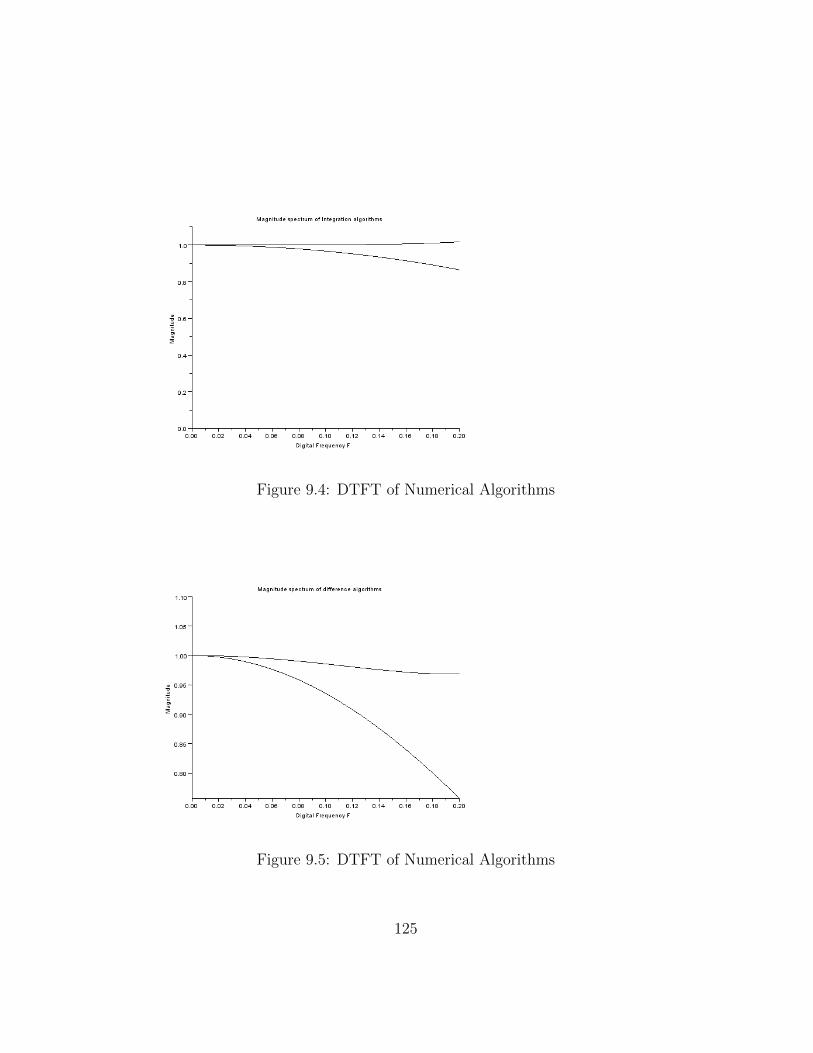
Figure 9.4: DTFT of Numerical Algorithms
Figure 9.5: DTFT of Numerical Algorithms
125
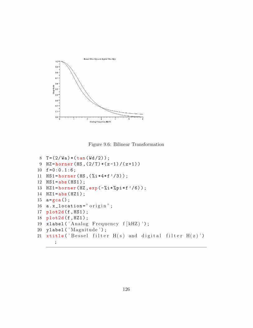
Figure 9.6: Bilinear Transformation
8 T=(2/Wa)*(tan(Wd/2));
9 HZ=horner(HS ,(2/T)*(z-1)/(z+1))
10 f=0:0.1:6;
11 HS1=horner(HS ,(%i*4*f’/3));
12 HS1=abs(HS1);
13 HZ1=horner(HZ,exp(-%i*%pi*f’/6));
14 HZ1=abs(HZ1);
15 a=gca();
16 a.x_location=” o r i g i n ”;17 plot2d(f,HS1);
18 plot2d(f,HZ1);
19 xlabel( ’ Analog Frequency f [ kHZ) ’ );20 ylabel( ’ Magnitude ’ );21 xtitle( ’ B e s s e l f i l t e r H( s ) and d i g i t a l f i l t e r H( z ) ’ )
;
126
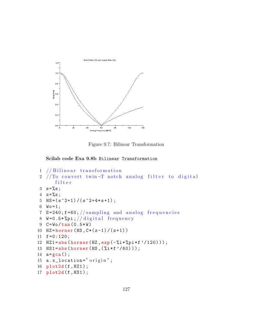
Figure 9.7: Bilinear Transformation
Scilab code Exa 9.8b Bilinear Transformation
1 // B i l i n e a r t r a n s f o r m a t i o n2 //To c o n v e r t twin−T notch ana l og f i l t e r to d i g i t a l
f i l t e r3 s=%s;
4 z=%z;
5 HS=(s^2+1)/(s^2+4*s+1);
6 Wo=1;
7 S=240;f=60; // sampl ing and ana l og f r e q u e n c i e s8 W=0.5* %pi;// d i g i t a l f r e q u e n c y9 C=Wo/tan (0.5*W)
10 HZ=horner(HS ,C*(z-1)/(z+1))
11 f=0:120;
12 HZ1=abs(horner(HZ ,exp(-%i*%pi*f ’/120)));
13 HS1=abs(horner(HS ,(%i*f’/60)));
14 a=gca();
15 a.x_location=” o r i g i n ”;16 plot2d(f,HZ1);
17 plot2d(f,HS1);
127
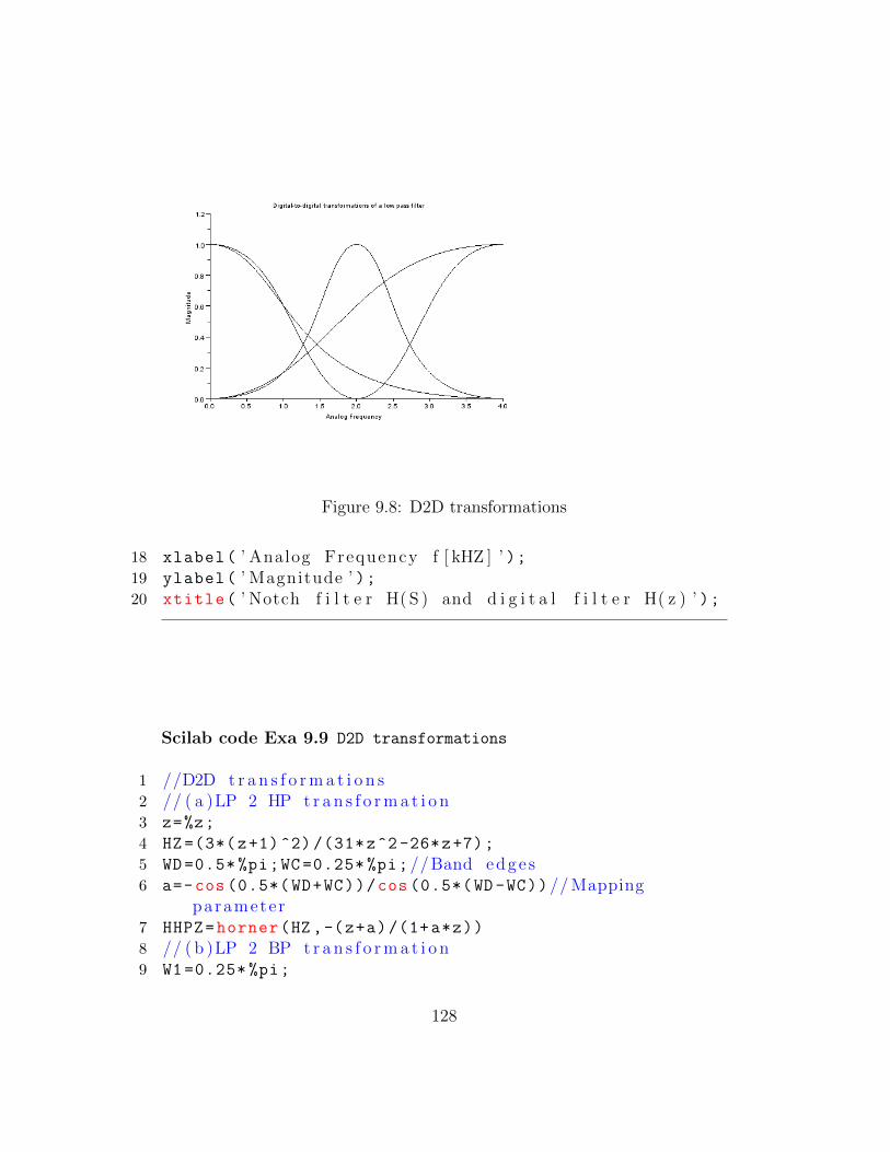
Figure 9.8: D2D transformations
18 xlabel( ’ Analog Frequency f [ kHZ ] ’ );19 ylabel( ’ Magnitude ’ );20 xtitle( ’ Notch f i l t e r H( S ) and d i g i t a l f i l t e r H( z ) ’ );
Scilab code Exa 9.9 D2D transformations
1 //D2D t r a n s f o r m a t i o n s2 // ( a )LP 2 HP t r a n s f o r m a t i o n3 z=%z;
4 HZ=(3*(z+1)^2) /(31*z^2-26*z+7);
5 WD=0.5* %pi;WC =0.25* %pi;//Band edge s6 a=-cos (0.5*( WD+WC))/cos (0.5*(WD-WC))// Mapping
parameter7 HHPZ=horner(HZ ,-(z+a)/(1+a*z))
8 // ( b )LP 2 BP t r a n s f o r m a t i o n9 W1 =0.25* %pi;
128
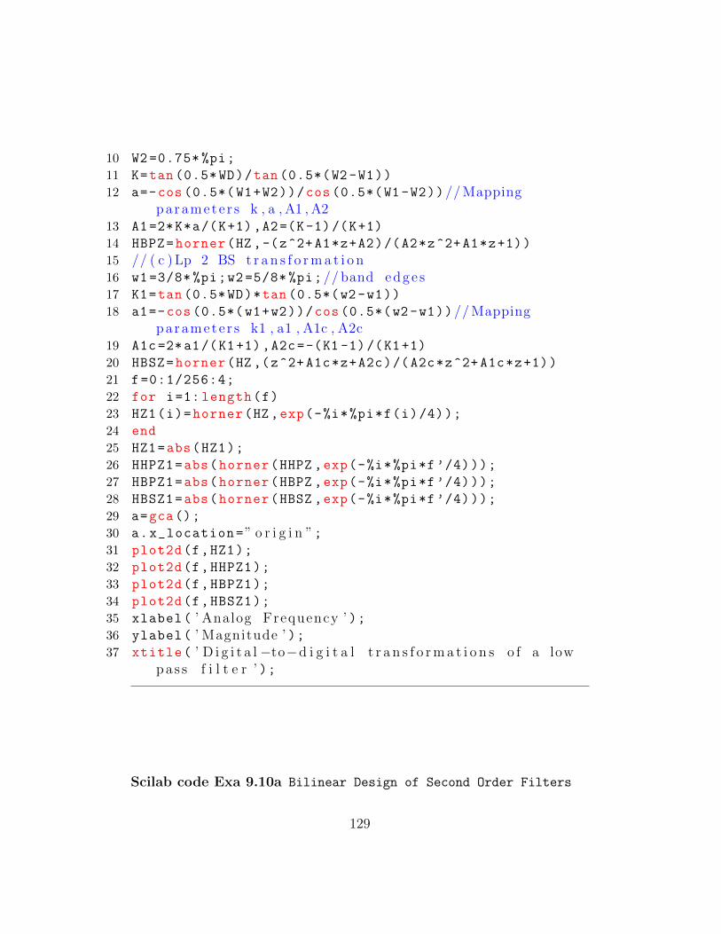
10 W2 =0.75* %pi;
11 K=tan (0.5*WD)/tan (0.5*(W2 -W1))
12 a=-cos (0.5*( W1+W2))/cos (0.5*(W1-W2))// Mappingparamete r s k , a , A1 , A2
13 A1=2*K*a/(K+1),A2=(K-1)/(K+1)
14 HBPZ=horner(HZ ,-(z^2+A1*z+A2)/(A2*z^2+A1*z+1))
15 // ( c ) Lp 2 BS t r a n s f o r m a t i o n16 w1=3/8* %pi;w2=5/8* %pi;// band edge s17 K1=tan (0.5*WD)*tan (0.5*(w2-w1))
18 a1=-cos (0.5*( w1+w2))/cos (0.5*(w2 -w1))// Mappingparamete r s k1 , a1 , A1c , A2c
19 A1c =2*a1/(K1+1),A2c=-(K1 -1)/(K1+1)
20 HBSZ=horner(HZ ,(z^2+A1c*z+A2c)/(A2c*z^2+A1c*z+1))
21 f=0:1/256:4;
22 for i=1: length(f)
23 HZ1(i)=horner(HZ ,exp(-%i*%pi*f(i)/4));
24 end
25 HZ1=abs(HZ1);
26 HHPZ1=abs(horner(HHPZ ,exp(-%i*%pi*f’/4)));
27 HBPZ1=abs(horner(HBPZ ,exp(-%i*%pi*f’/4)));
28 HBSZ1=abs(horner(HBSZ ,exp(-%i*%pi*f’/4)));
29 a=gca();
30 a.x_location=” o r i g i n ”;31 plot2d(f,HZ1);
32 plot2d(f,HHPZ1);
33 plot2d(f,HBPZ1);
34 plot2d(f,HBSZ1);
35 xlabel( ’ Analog Frequency ’ );36 ylabel( ’ Magnitude ’ );37 xtitle( ’ D i g i t a l −to−d i g i t a l t r a n s f o r m a t i o n s o f a low
pas s f i l t e r ’ );
Scilab code Exa 9.10a Bilinear Design of Second Order Filters
129
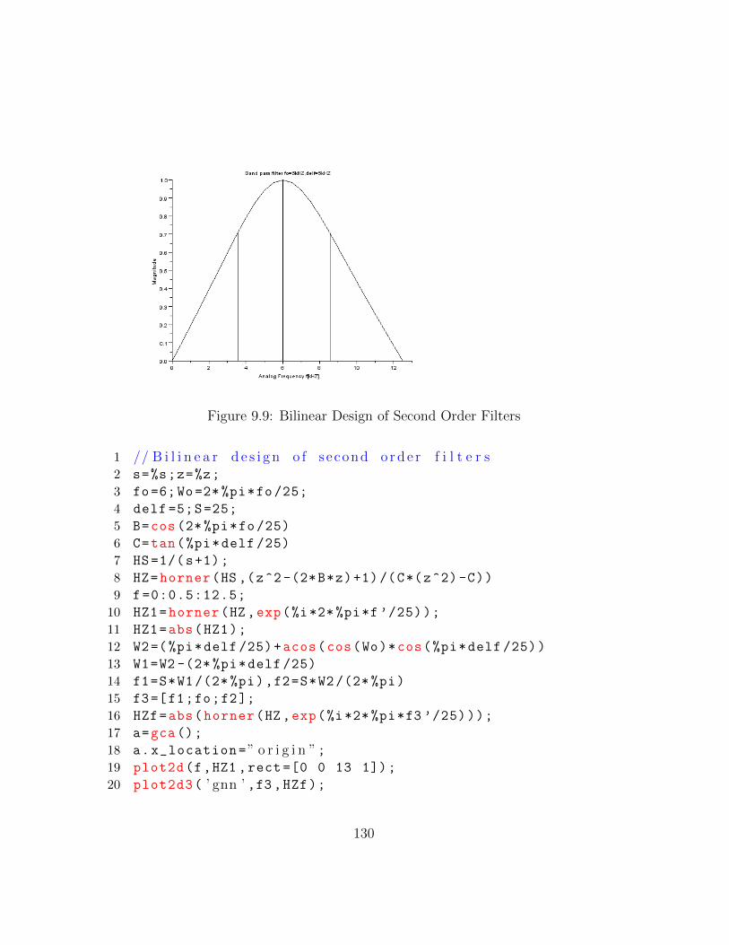
Figure 9.9: Bilinear Design of Second Order Filters
1 // B i l i n e a r d e s i g n o f s econd o r d e r f i l t e r s2 s=%s;z=%z;
3 fo=6;Wo=2* %pi*fo/25;
4 delf =5;S=25;
5 B=cos(2*%pi*fo/25)
6 C=tan(%pi*delf /25)
7 HS=1/(s+1);
8 HZ=horner(HS ,(z^2 -(2*B*z)+1)/(C*(z^2)-C))
9 f=0:0.5:12.5;
10 HZ1=horner(HZ,exp(%i*2* %pi*f’/25));
11 HZ1=abs(HZ1);
12 W2=(%pi*delf /25)+acos(cos(Wo)*cos(%pi*delf /25))
13 W1=W2 -(2* %pi*delf /25)
14 f1=S*W1/(2* %pi),f2=S*W2/(2* %pi)
15 f3=[f1;fo;f2];
16 HZf=abs(horner(HZ ,exp(%i*2*%pi*f3 ’/25)));
17 a=gca();
18 a.x_location=” o r i g i n ”;19 plot2d(f,HZ1 ,rect =[0 0 13 1]);
20 plot2d3( ’ gnn ’ ,f3 ,HZf);
130
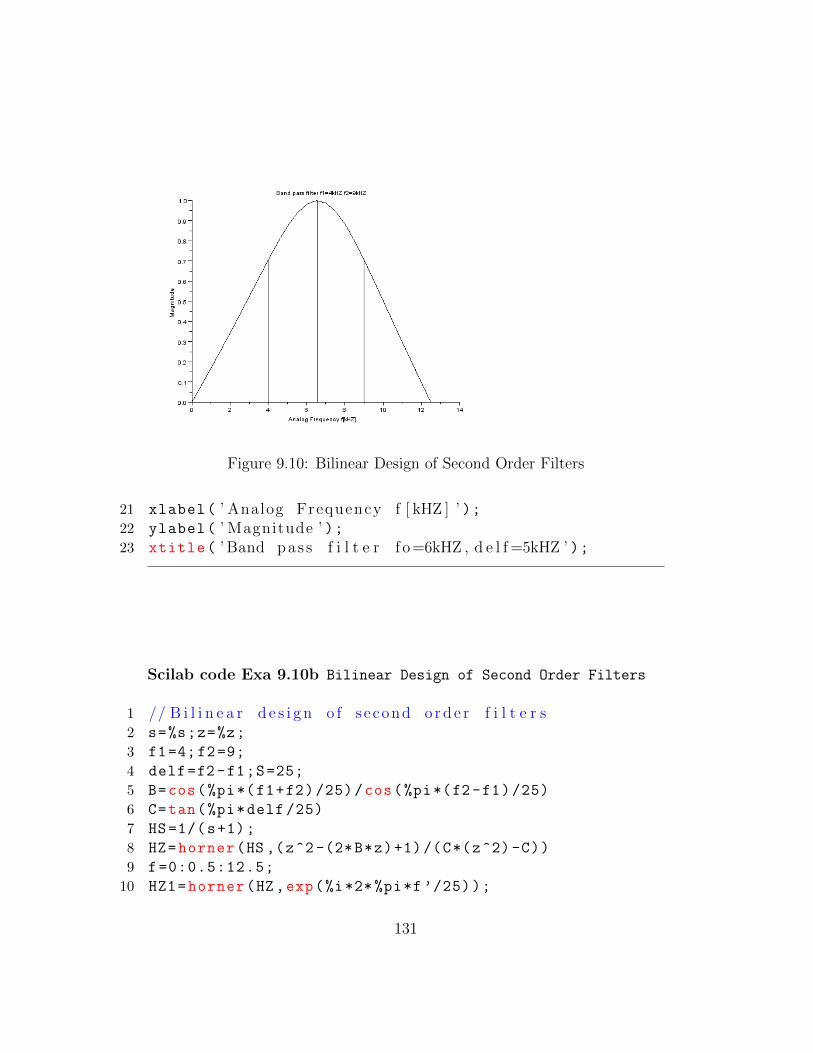
Figure 9.10: Bilinear Design of Second Order Filters
21 xlabel( ’ Analog Frequency f [ kHZ ] ’ );22 ylabel( ’ Magnitude ’ );23 xtitle( ’ Band pas s f i l t e r f o =6kHZ , d e l f =5kHZ ’ );
Scilab code Exa 9.10b Bilinear Design of Second Order Filters
1 // B i l i n e a r d e s i g n o f s econd o r d e r f i l t e r s2 s=%s;z=%z;
3 f1=4;f2=9;
4 delf=f2-f1;S=25;
5 B=cos(%pi*(f1+f2)/25)/cos(%pi*(f2 -f1)/25)
6 C=tan(%pi*delf /25)
7 HS=1/(s+1);
8 HZ=horner(HS ,(z^2 -(2*B*z)+1)/(C*(z^2)-C))
9 f=0:0.5:12.5;
10 HZ1=horner(HZ,exp(%i*2* %pi*f’/25));
131
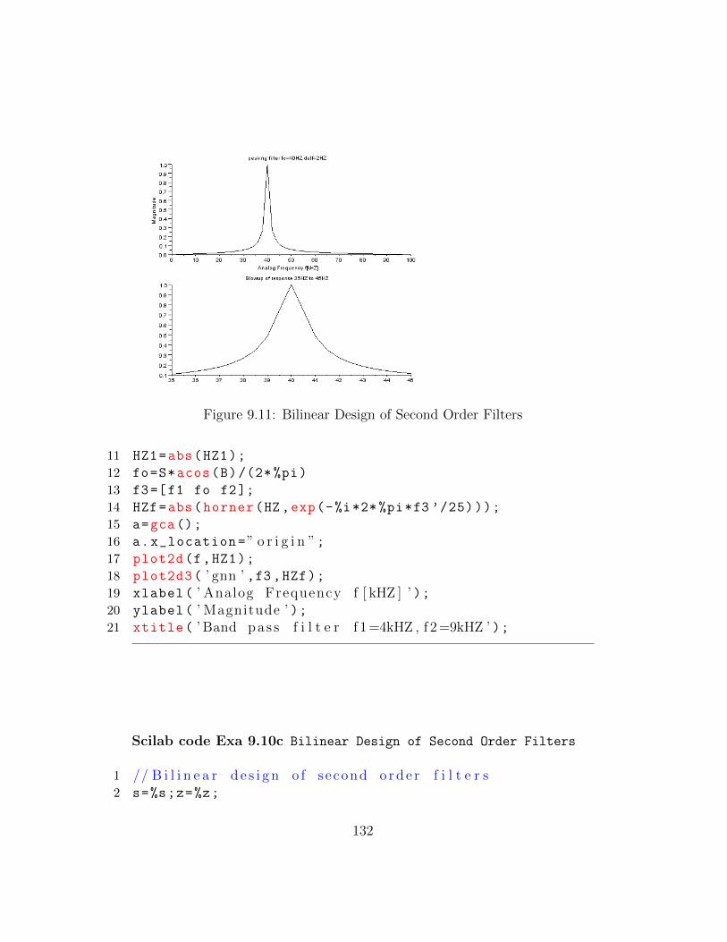
Figure 9.11: Bilinear Design of Second Order Filters
11 HZ1=abs(HZ1);
12 fo=S*acos(B)/(2* %pi)
13 f3=[f1 fo f2];
14 HZf=abs(horner(HZ ,exp(-%i*2*%pi*f3 ’/25)));
15 a=gca();
16 a.x_location=” o r i g i n ”;17 plot2d(f,HZ1);
18 plot2d3( ’ gnn ’ ,f3 ,HZf);19 xlabel( ’ Analog Frequency f [ kHZ ] ’ );20 ylabel( ’ Magnitude ’ );21 xtitle( ’ Band pas s f i l t e r f 1 =4kHZ , f 2 =9kHZ ’ );
Scilab code Exa 9.10c Bilinear Design of Second Order Filters
1 // B i l i n e a r d e s i g n o f s econd o r d e r f i l t e r s2 s=%s;z=%z;
132
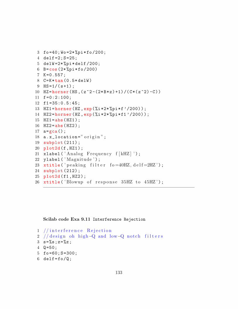
3 fo=40;Wo=2*%pi*fo /200;
4 delf =2;S=25;
5 delW =2*%pi*delf /200;
6 B=cos(2*%pi*fo/200)
7 K=0.557;
8 C=K*tan (0.5* delW)
9 HS=1/(s+1);
10 HZ=horner(HS ,(z^2 -(2*B*z)+1)/(C*(z^2)-C))
11 f=0:2:100;
12 f1 =35:0.5:45;
13 HZ1=horner(HZ,exp(%i*2* %pi*f ’/200));
14 HZ2=horner(HZ,exp(%i*2* %pi*f1 ’/200));
15 HZ1=abs(HZ1);
16 HZ2=abs(HZ2);
17 a=gca();
18 a.x_location=” o r i g i n ”;19 subplot (211);
20 plot2d(f,HZ1);
21 xlabel( ’ Analog Frequency f [ kHZ ] ’ );22 ylabel( ’ Magnitude ’ );23 xtitle( ’ p eak ing f i l t e r f o =40HZ, d e l f =2HZ ’ );24 subplot (212);
25 plot2d(f1,HZ2);
26 xtitle( ’ Blowup o f r e s p o n s e 35HZ to 45HZ ’ );
Scilab code Exa 9.11 Interference Rejection
1 // i n t e r f e r e n c e R e j e c t i o n2 // d e s i g n oh high−Q and low−Q notch f i l t e r s3 s=%s;z=%z;
4 Q=50;
5 fo=60;S=300;
6 delf=fo/Q;
133
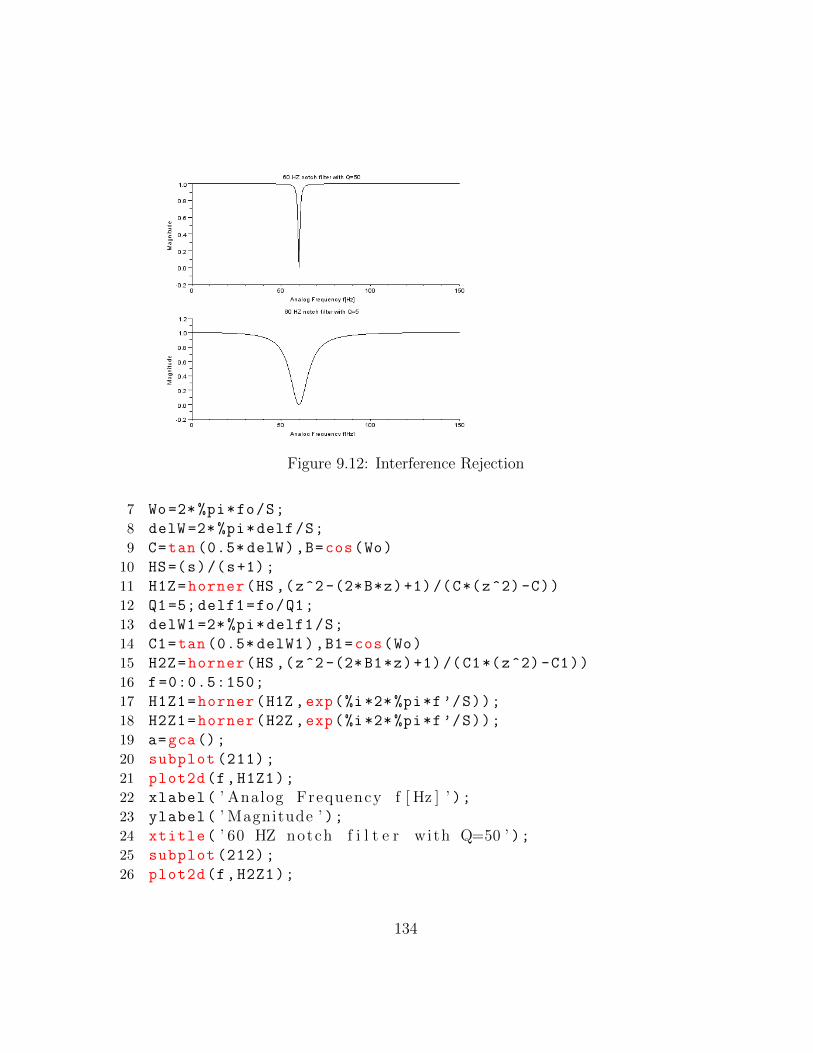
Figure 9.12: Interference Rejection
7 Wo=2*%pi*fo/S;
8 delW =2*%pi*delf/S;
9 C=tan (0.5* delW),B=cos(Wo)
10 HS=(s)/(s+1);
11 H1Z=horner(HS ,(z^2-(2*B*z)+1)/(C*(z^2)-C))
12 Q1=5; delf1=fo/Q1;
13 delW1 =2* %pi*delf1/S;
14 C1=tan (0.5* delW1),B1=cos(Wo)
15 H2Z=horner(HS ,(z^2-(2*B1*z)+1)/(C1*(z^2)-C1))
16 f=0:0.5:150;
17 H1Z1=horner(H1Z ,exp(%i*2*%pi*f’/S));
18 H2Z1=horner(H2Z ,exp(%i*2*%pi*f’/S));
19 a=gca();
20 subplot (211);
21 plot2d(f,H1Z1);
22 xlabel( ’ Analog Frequency f [ Hz ] ’ );23 ylabel( ’ Magnitude ’ );24 xtitle( ’ 60 HZ notch f i l t e r with Q=50 ’ );25 subplot (212);
26 plot2d(f,H2Z1);
134
Figure 9.13: IIR Filter Design
27 xlabel( ’ Analog Frequency f [ Hz ] ’ );28 ylabel( ’ Magnitude ’ );29 xtitle( ’ 60 HZ notch f i l t e r with Q=5 ’ );
Scilab code Exa 9.12 IIR Filter Design
1 // IIR f i l t e r d e s i g n2 // Des ign o f chebyshev IIR f i l t e r with f o l l o w i n g
s p e c i f i c a t i o n s3 fp1 =1.6; fp2 =1.8; fs1 =3.2; fs2 =4.8; // pas s band edge s4 Ap=2;As=20;S=12;
5 s=%s;z=%z;
6 // ( a ) I n d i r e c t B i l i n e a r d e s i g n7 W=2*%pi*[fp1 fp2 fs1 fs2]/S
8 C=2;
135
9 omega =2* tan (0.5*W’);// prewarp ing each band edgef r e q u e n c y
10 epsilon=sqrt (10^(0.1* Ap) -1);
11 n=acosh (((10^(0.1* As) -1)/epsilon ^2) ^1/2)/(acosh(fs1/
fp1));
12 n=ceil(n)
13 alpha =(1/n)*asinh (1/ epsilon);
14 for i=1:n
15 B(i)=(2*i-1)*%pi /(2*n);
16 end
17 for i=1:n
18 p(i)=-sinh(alpha)*sin(B(i))+%i*cosh(alpha)*cos(B
(i));
19 end
20 Qs=1;
21 for i=1:n
22 Qs=Qs*(s-p(i))
23 end
24 Qo =0.1634;
25 HPS=Qo/Qs
26 HBPS=horner(HPS ,(s^2+1.5045^2) /(s*1.202))
27 HZ=horner(HBPS ,2*(z-1)/(z+1))
28 f=0:0.001:0.5;
29 HZF=abs(horner(HZ ,exp(%i*2*%pi*f’)));
30 HBPF=abs(horner(HBPS ,%i*2*%pi*f’));
31 a=gca();
32 plot2d(f,HZF);
33 plot2d(f,HBPF);
34 xlabel( ’ Analog Frequency ’ );35 ylabel( ’ magnitude ’ );36 xtitle( ’ band pas s f i l t e r d e s i g n e d by the b i l i n e a r
t r a n s f o r m a t i o n ’ );
136
Chapter 10
Design of FIR filters
Scilab code Exa 10.2 Truncation and Windowing
1 // Truncat ion and Windowing2 // ( a )N=9 , B a r l e t t Window .3 z=%z;
4 Fc =0.25;
5 n=-4:4;
6 hn=2*Fc*(sinc (0.5*n’*%pi))
7 Wn=1-(2* abs(n’))/8 // B a r l e t t window8 hwn=hn.*Wn
9 Hcz =0;
10 for i=1: length(hwn)
11 Hcz=Hcz+hwn(i)*(z^((2-i)));
12 end
13 Hcz // i n d i c a t e s d e l a y o f 0 . 1 5 ms14 // ( b )N=6 , vonhann Window15 n1= -2.5:2.5;
16 hn1 =2*Fc*(sinc (0.5*n1 ’*%pi))
17 Wn1 =0.5+0.5*( cos (0.4* %pi*n1 ’))// Vonhann window18 hwn1=hn1.*Wn1
19 Hcz1 =0;
20 for i=1: length(hwn1)
21 Hcz1=Hcz1+hwn1(i)*(z^((2-i)));
137
22 end
23 Hcz1 // 1 s t sample o f hwn i s 0 hence d e l a y i s 1 . 5 ms
Scilab code Exa 10.3ab FIR lowpass Filter design
1 //FIR f i l t e r d e s i g n u s i n g windows2 // ( a ) Des ign o f FIR f i l t e r to meet f o l l o w i n g
s p e c i f i c a t i o n s3 fp=2;fs=4;Ap=2;As=40;S=20;
4 Fp=fp/S;Fs=fs/S;
5 Fc =0.15;
6 z=%z;
7 N1 =3.21/(Fs -Fp);
8 N1=ceil(N1)
9 N2 =5.71/(Fs -Fp);
10 N2=ceil(N2)
11 n1= -16:16;
12 n2 = -28.5:1:28.5;
13 hn1 =2*Fc*(sinc (2*Fc*n1 ’));
14 hn2 =2*Fc*(sinc (2*Fc*n2 ’));
15 Wn1 =0.5+0.5*( cos(2*%pi*n1 ’/(N1 -1)));// Vonhann window16 Wn2 =0.42+0.5*( cos(2*%pi*n2 ’/(N2 -1)))+0.08*( cos (4*%pi
*n2 ’/(N2 -1)));// Blackman window17 hwn1=abs(hn1.*Wn1);
18 hwn2=abs(hn2.*Wn2);
19 [hwn1F ,fr1]=frmag(hwn1 ,256);
20 [hwn2F ,fr2]=frmag(hwn2 ,256);
21 hwn1F1 =20* log10(hwn1F);
22 hwn2F1 =20* log10(hwn2F);
23 plot2d(fr1 ,hwn1F1);
24 plot2d(fr2(1: length(fr2) -2),hwn2F1 (1: length(fr2) -2))
;
25 xlabel( ’ D i g i t a l f r e q u e n c y ’ );26 ylabel( ’ Magnitude [ dB ] ’ );27 title( ’Low pas s f i l t e r u s i n g vonhann and Blackmann
138
windows Fc =0.15 , vonhann N=33 , Blackman N=58 ’ );28 // ( b ) Minimum l e n g t h d e s i g n29 Fcv =0.1313;
30 Fcb =0.1278;
31 Nv=23;Nb=29;
32 nv= -11:11;
33 nb= -14:14;
34 hnv =2*Fcv*(sinc (2*Fcv*nv ’));
35 hnb =2*Fcb*(sinc (2*Fcb*nb ’));
36 Wnv =0.5+0.5*( cos(2*%pi*nv ’/(Nv -1)));// Vonhann window37 Wnb =0.42+0.5*( cos(2*%pi*nb ’/(Nb -1)))+0.08*( cos (4*%pi
*nb ’/(Nb -1)));// Blackman window38 hwnv=abs(hnv.*Wnv);
39 hwnb=abs(hnb.*Wnb);
40 [hwnvF ,frv]=frmag(hwnv ,256);
41 [hwnbF ,frb]=frmag(hwnb ,256);
42 hwnvF =20* log10(hwnvF);
43 hwnbF =20* log10(hwnbF);
44 b=gca();
45 xset( ’ window ’ ,2);46 plot(frv ,hwnvF);
47 plot(frb ,hwnbF);
48 xlabel( ’ D i g i t a l f r e q u e n c y ’ );49 ylabel( ’ Magnitude [ dB ] ’ );50 title( ’ Vonhann Fc =0.1313 , Minimum N=23 , Blackmann Fc
=0.1278 , Minimum N=29 ’ );
Scilab code Exa 10.3cd FIR filter Design
1 // Des ign o f h igh pas s FIR f i l t e r with s p e c i f i c a t i o n s2 // fp=4kHZ ; f s =2kHZ ; Ap=2dB ; As=40dB
139
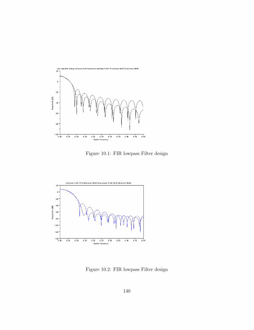
Figure 10.1: FIR lowpass Filter design
Figure 10.2: FIR lowpass Filter design
140
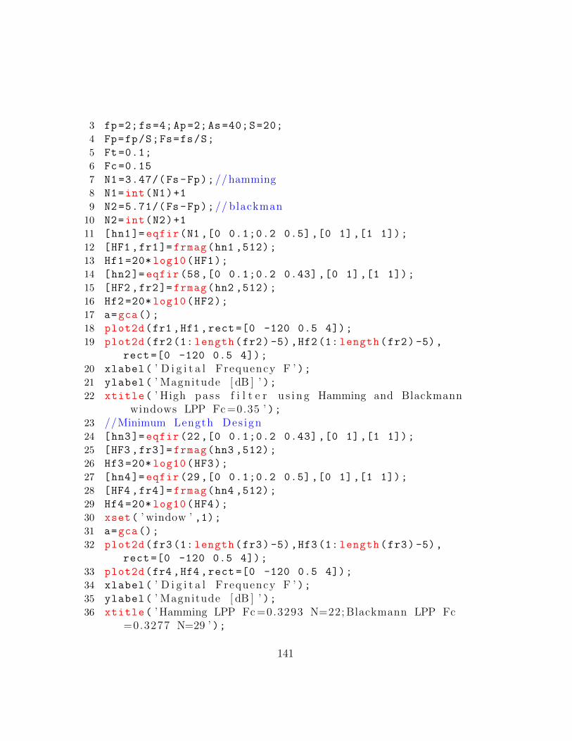
3 fp=2;fs=4;Ap=2;As=40;S=20;
4 Fp=fp/S;Fs=fs/S;
5 Ft=0.1;
6 Fc=0.15
7 N1 =3.47/(Fs -Fp);//hamming8 N1=int(N1)+1
9 N2 =5.71/(Fs -Fp);// blackman10 N2=int(N2)+1
11 [hn1]= eqfir(N1 ,[0 0.1;0.2 0.5] ,[0 1],[1 1]);
12 [HF1 ,fr1]=frmag(hn1 ,512);
13 Hf1 =20* log10(HF1);
14 [hn2]= eqfir (58,[0 0.1;0.2 0.43] ,[0 1],[1 1]);
15 [HF2 ,fr2]=frmag(hn2 ,512);
16 Hf2 =20* log10(HF2);
17 a=gca();
18 plot2d(fr1 ,Hf1 ,rect =[0 -120 0.5 4]);
19 plot2d(fr2(1: length(fr2) -5),Hf2(1: length(fr2) -5),
rect =[0 -120 0.5 4]);
20 xlabel( ’ D i g i t a l Frequency F ’ );21 ylabel( ’ Magnitude [ dB ] ’ );22 xtitle( ’ High pas s f i l t e r u s i n g Hamming and Blackmann
windows LPP Fc =0.35 ’ );23 //Minimum Length Des ign24 [hn3]= eqfir (22,[0 0.1;0.2 0.43] ,[0 1],[1 1]);
25 [HF3 ,fr3]=frmag(hn3 ,512);
26 Hf3 =20* log10(HF3);
27 [hn4]= eqfir (29,[0 0.1;0.2 0.5] ,[0 1],[1 1]);
28 [HF4 ,fr4]=frmag(hn4 ,512);
29 Hf4 =20* log10(HF4);
30 xset( ’ window ’ ,1);31 a=gca();
32 plot2d(fr3(1: length(fr3) -5),Hf3(1: length(fr3) -5),
rect =[0 -120 0.5 4]);
33 plot2d(fr4 ,Hf4 ,rect =[0 -120 0.5 4]);
34 xlabel( ’ D i g i t a l Frequency F ’ );35 ylabel( ’ Magnitude [ dB ] ’ );36 xtitle( ’Hamming LPP Fc =0.3293 N=22; Blackmann LPP Fc
=0.3277 N=29 ’ );
141
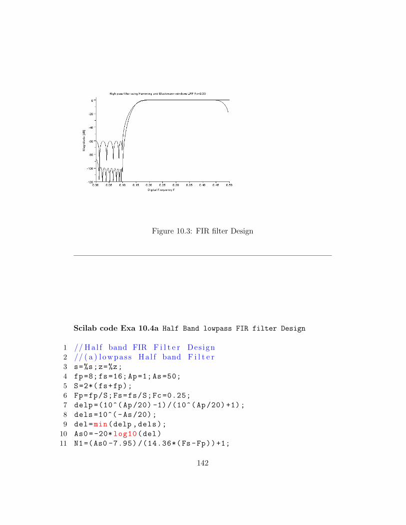
Figure 10.3: FIR filter Design
Scilab code Exa 10.4a Half Band lowpass FIR filter Design
1 // Ha l f band FIR F i l t e r Des ign2 // ( a ) l owpas s Ha l f band F i l t e r3 s=%s;z=%z;
4 fp=8;fs=16;Ap=1;As=50;
5 S=2*(fs+fp);
6 Fp=fp/S;Fs=fs/S;Fc =0.25;
7 delp =(10^( Ap/20) -1)/(10^( Ap/20) +1);
8 dels =10^( -As/20);
9 del=min(delp ,dels);
10 As0=-20* log10(del)
11 N1=(As0 -7.95) /(14.36*(Fs -Fp))+1;
142
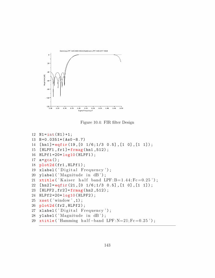
Figure 10.4: FIR filter Design
12 N1=int(N1)+1;
13 B=0.0351*(As0 -8.7)
14 [hn1]= eqfir (19,[0 1/6;1/3 0.5] ,[1 0],[1 1]);
15 [HLPF1 ,fr1]=frmag(hn1 ,512);
16 HLPf1 =20* log10(HLPF1);
17 a=gca();
18 plot2d(fr1 ,HLPf1);
19 xlabel( ’ D i g i t a l Frequency ’ );20 ylabel( ’ Magnitude i n dB ’ );21 xtitle( ’ K a i s e r h a l f band LPF :B=1 .44 ; Fc =0.25 ’ );22 [hn2]= eqfir (21,[0 1/6;1/3 0.5] ,[1 0],[1 1]);
23 [HLPF2 ,fr2]=frmag(hn2 ,512);
24 HLPf2 =20* log10(HLPF2);
25 xset( ’ window ’ ,1);26 plot2d(fr2 ,HLPf2);
27 xlabel( ’ D i g i t a l Frequency ’ );28 ylabel( ’ Magnitude i n dB ’ );29 xtitle( ’Hamming h a l f −band LPF :N=21; Fc =0.25 ’ );
143
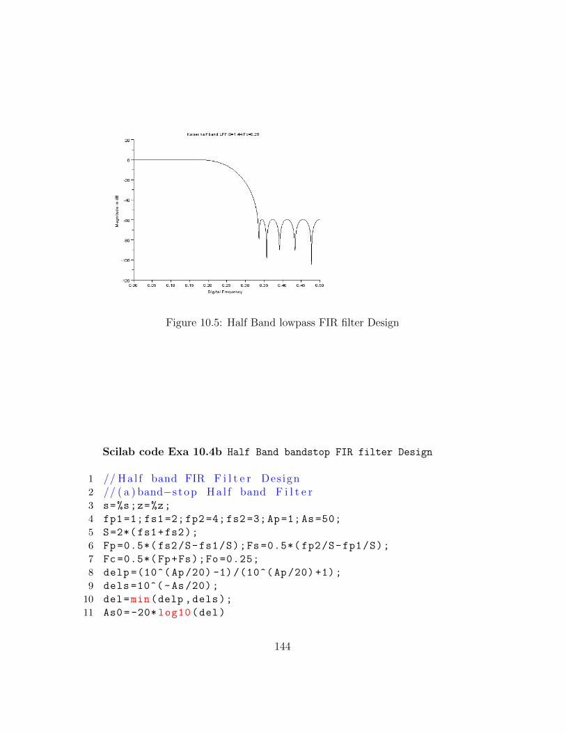
Figure 10.5: Half Band lowpass FIR filter Design
Scilab code Exa 10.4b Half Band bandstop FIR filter Design
1 // Ha l f band FIR F i l t e r Des ign2 // ( a ) band−s t op Ha l f band F i l t e r3 s=%s;z=%z;
4 fp1 =1;fs1=2;fp2 =4;fs2=3;Ap=1;As=50;
5 S=2*( fs1+fs2);
6 Fp =0.5*( fs2/S-fs1/S);Fs =0.5*( fp2/S-fp1/S);
7 Fc =0.5*( Fp+Fs);Fo =0.25;
8 delp =(10^( Ap/20) -1)/(10^( Ap/20) +1);
9 dels =10^( -As/20);
10 del=min(delp ,dels);
11 As0=-20* log10(del)
144
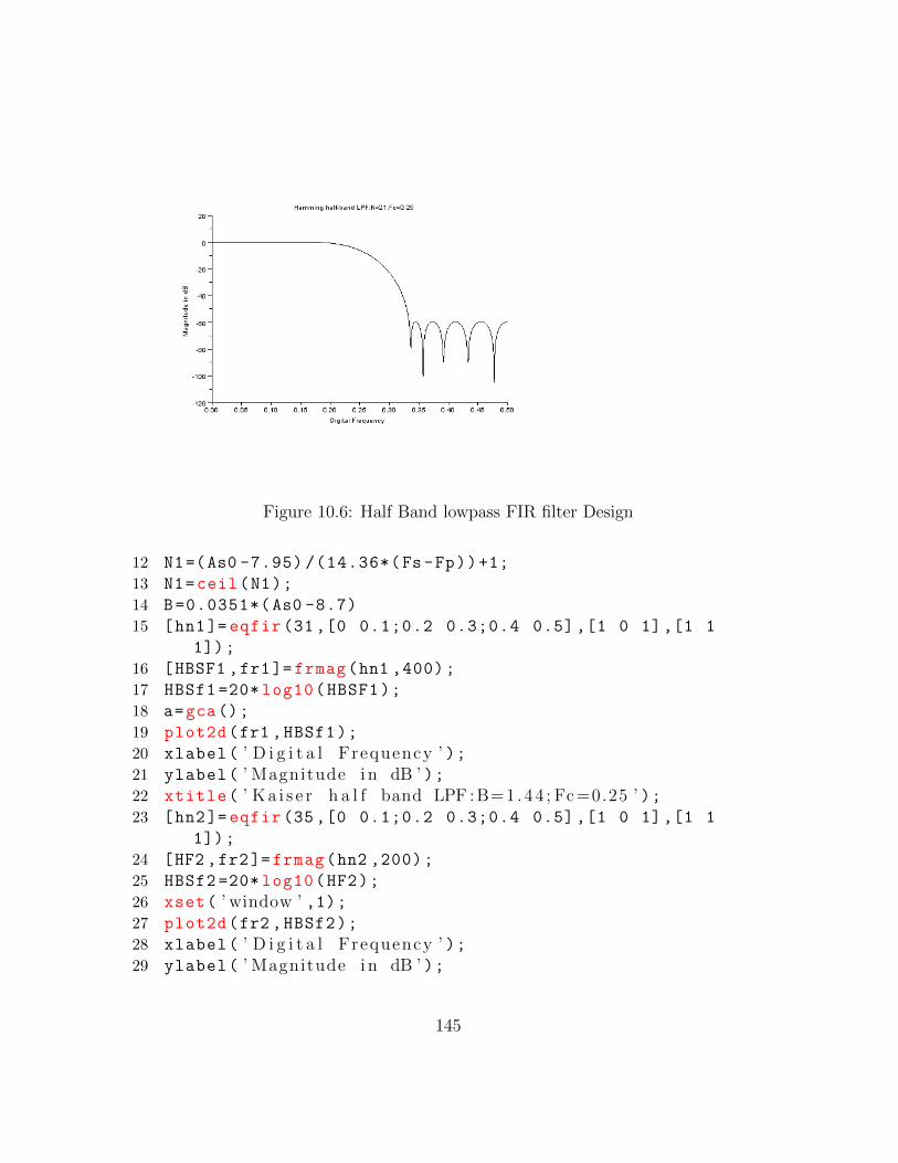
Figure 10.6: Half Band lowpass FIR filter Design
12 N1=(As0 -7.95) /(14.36*(Fs -Fp))+1;
13 N1=ceil(N1);
14 B=0.0351*(As0 -8.7)
15 [hn1]= eqfir (31,[0 0.1;0.2 0.3;0.4 0.5] ,[1 0 1],[1 1
1]);
16 [HBSF1 ,fr1]=frmag(hn1 ,400);
17 HBSf1 =20* log10(HBSF1);
18 a=gca();
19 plot2d(fr1 ,HBSf1);
20 xlabel( ’ D i g i t a l Frequency ’ );21 ylabel( ’ Magnitude i n dB ’ );22 xtitle( ’ K a i s e r h a l f band LPF :B=1 .44 ; Fc =0.25 ’ );23 [hn2]= eqfir (35,[0 0.1;0.2 0.3;0.4 0.5] ,[1 0 1],[1 1
1]);
24 [HF2 ,fr2]=frmag(hn2 ,200);
25 HBSf2 =20* log10(HF2);
26 xset( ’ window ’ ,1);27 plot2d(fr2 ,HBSf2);
28 xlabel( ’ D i g i t a l Frequency ’ );29 ylabel( ’ Magnitude i n dB ’ );
145
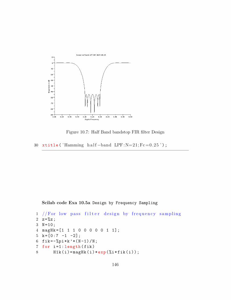
Figure 10.7: Half Band bandstop FIR filter Design
30 xtitle( ’Hamming h a l f −band LPF :N=21; Fc =0.25 ’ );
Scilab code Exa 10.5a Design by Frequency Sampling
1 // For low pas s f i l t e r d e s i g n by f r e q u e n c y sampl ing2 z=%z;
3 N=10;
4 magHk =[1 1 1 0 0 0 0 0 1 1];
5 k=[0:7 -1 -2];
6 fik=-%pi*k’*(N-1)/N;
7 for i=1: length(fik)
8 H1k(i)=magHk(i)*exp(%i*fik(i));
146
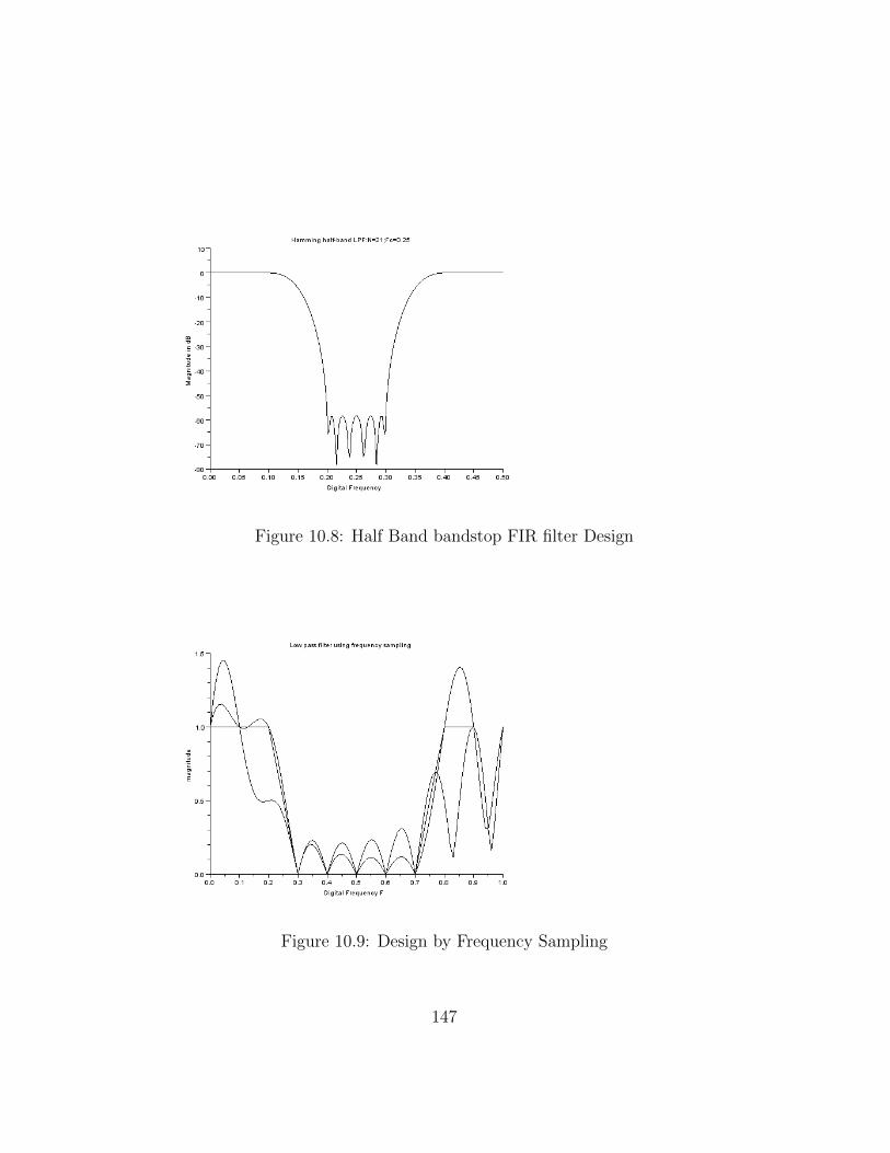
Figure 10.8: Half Band bandstop FIR filter Design
Figure 10.9: Design by Frequency Sampling
147
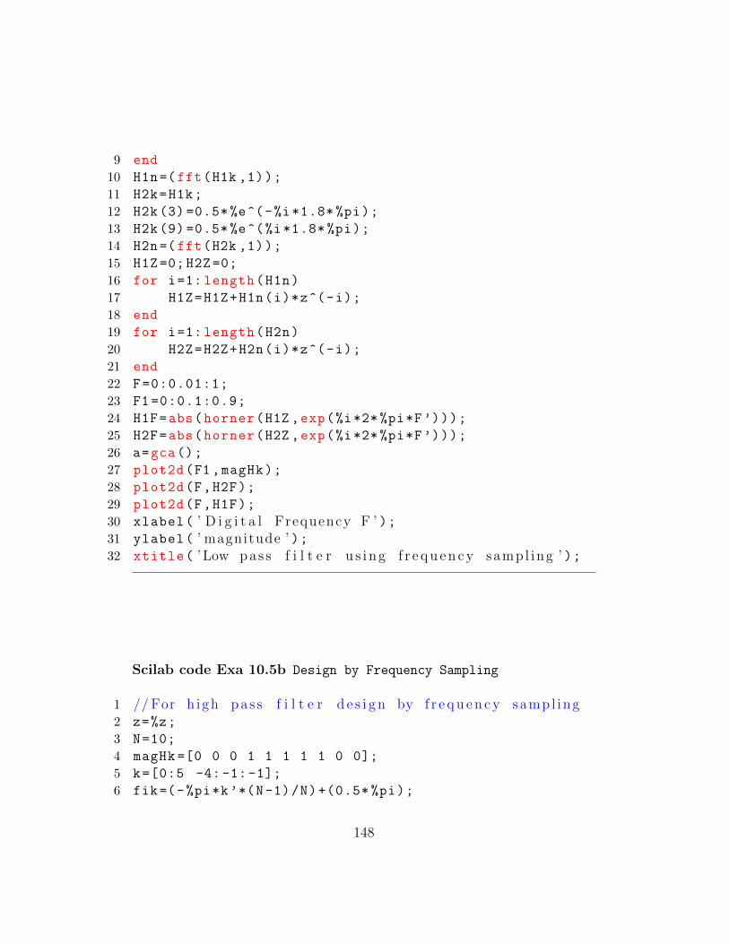
9 end
10 H1n=(fft(H1k ,1));
11 H2k=H1k;
12 H2k (3) =0.5*%e^(-%i*1.8* %pi);
13 H2k (9) =0.5*%e^(%i*1.8* %pi);
14 H2n=(fft(H2k ,1));
15 H1Z =0;H2Z=0;
16 for i=1: length(H1n)
17 H1Z=H1Z+H1n(i)*z^(-i);
18 end
19 for i=1: length(H2n)
20 H2Z=H2Z+H2n(i)*z^(-i);
21 end
22 F=0:0.01:1;
23 F1 =0:0.1:0.9;
24 H1F=abs(horner(H1Z ,exp(%i*2*%pi*F’)));
25 H2F=abs(horner(H2Z ,exp(%i*2*%pi*F’)));
26 a=gca();
27 plot2d(F1,magHk);
28 plot2d(F,H2F);
29 plot2d(F,H1F);
30 xlabel( ’ D i g i t a l Frequency F ’ );31 ylabel( ’ magnitude ’ );32 xtitle( ’Low pas s f i l t e r u s i n g f r e q u e n c y sampl ing ’ );
Scilab code Exa 10.5b Design by Frequency Sampling
1 // For h igh pas s f i l t e r d e s i g n by f r e q u e n c y sampl ing2 z=%z;
3 N=10;
4 magHk =[0 0 0 1 1 1 1 1 0 0];
5 k=[0:5 -4:-1:-1];
6 fik=(-%pi*k’*(N-1)/N)+(0.5* %pi);
148
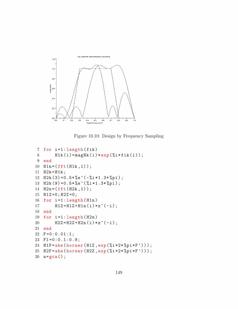
Figure 10.10: Design by Frequency Sampling
7 for i=1: length(fik)
8 H1k(i)=magHk(i)*exp(%i*fik(i));
9 end
10 H1n=(fft(H1k ,1));
11 H2k=H1k;
12 H2k (3) =0.5*%e^(-%i*1.3* %pi);
13 H2k (9) =0.5*%e^(%i*1.3* %pi);
14 H2n=(fft(H2k ,1));
15 H1Z =0;H2Z=0;
16 for i=1: length(H1n)
17 H1Z=H1Z+H1n(i)*z^(-i);
18 end
19 for i=1: length(H2n)
20 H2Z=H2Z+H2n(i)*z^(-i);
21 end
22 F=0:0.01:1;
23 F1 =0:0.1:0.9;
24 H1F=abs(horner(H1Z ,exp(%i*2*%pi*F’)));
25 H2F=abs(horner(H2Z ,exp(%i*2*%pi*F’)));
26 a=gca();
149
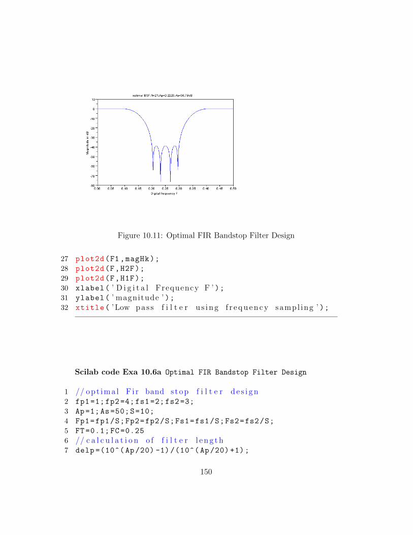
Figure 10.11: Optimal FIR Bandstop Filter Design
27 plot2d(F1,magHk);
28 plot2d(F,H2F);
29 plot2d(F,H1F);
30 xlabel( ’ D i g i t a l Frequency F ’ );31 ylabel( ’ magnitude ’ );32 xtitle( ’Low pas s f i l t e r u s i n g f r e q u e n c y sampl ing ’ );
Scilab code Exa 10.6a Optimal FIR Bandstop Filter Design
1 // opt ima l F i r band s top f i l t e r d e s i g n2 fp1 =1;fp2=4;fs1 =2;fs2=3;
3 Ap=1;As=50;S=10;
4 Fp1=fp1/S;Fp2=fp2/S;Fs1=fs1/S;Fs2=fs2/S;
5 FT=0.1;FC=0.25
6 // c a l c u l a t i o n o f f i l t e r l e n g t h7 delp =(10^( Ap/20) -1)/(10^( Ap/20) +1);
150
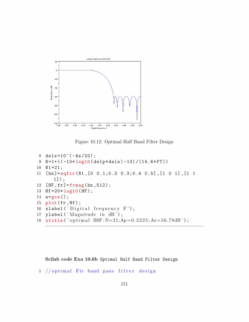
Figure 10.12: Optimal Half Band Filter Design
8 dels =10^( -As/20);
9 N=1+(( -10* log10(delp*dels) -13) /(14.6* FT))
10 N1=21;
11 [hn]= eqfir(N1 ,[0 0.1;0.2 0.3;0.4 0.5] ,[1 0 1],[1 1
1]);
12 [HF ,fr]= frmag(hn ,512);
13 Hf=20* log10(HF);
14 a=gca();
15 plot(fr,Hf);
16 xlabel( ’ D i g i t a l f r e q u e n c y F ’ );17 ylabel( ’ Magnitude i n dB ’ );18 xtitle( ’ op t ima l BSF :N=21;Ap=0 .2225 ; As =56.79dB ’ );
Scilab code Exa 10.6b Optimal Half Band Filter Design
1 // opt ima l F i r band pas s f i l t e r d e s i g n
151
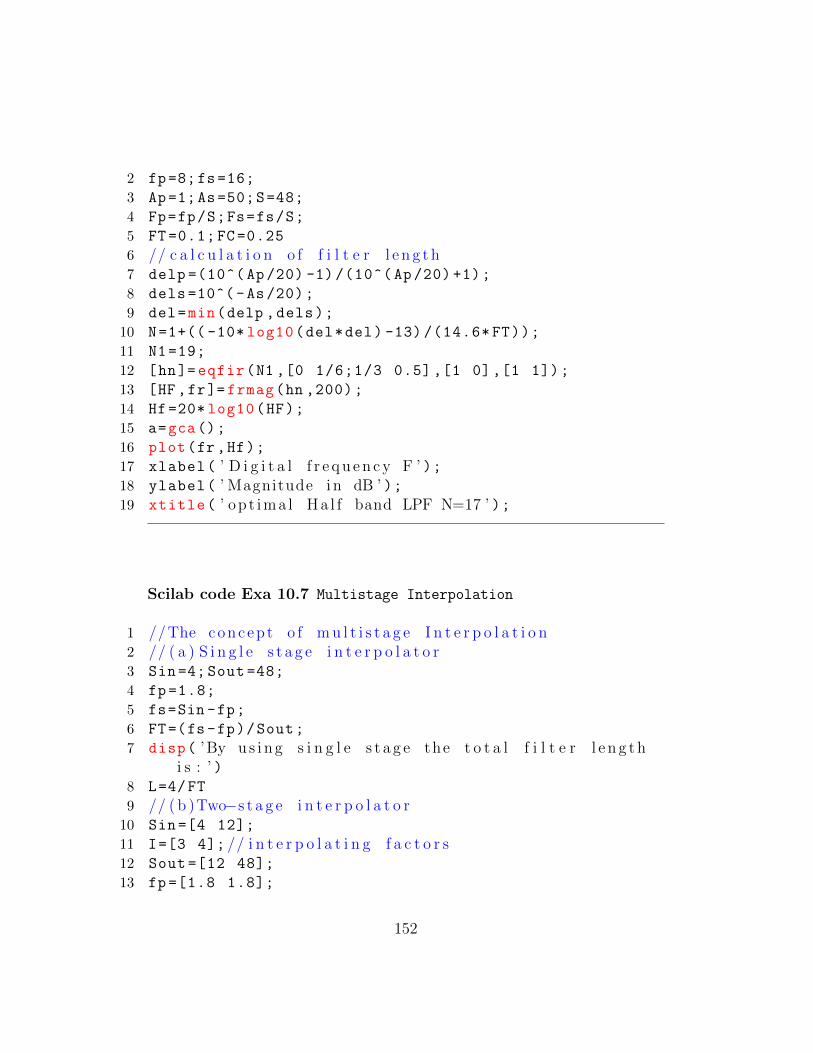
2 fp=8;fs=16;
3 Ap=1;As=50;S=48;
4 Fp=fp/S;Fs=fs/S;
5 FT=0.1;FC=0.25
6 // c a l c u l a t i o n o f f i l t e r l e n g t h7 delp =(10^( Ap/20) -1)/(10^( Ap/20) +1);
8 dels =10^( -As/20);
9 del=min(delp ,dels);
10 N=1+(( -10* log10(del*del) -13) /(14.6* FT));
11 N1=19;
12 [hn]= eqfir(N1 ,[0 1/6;1/3 0.5] ,[1 0],[1 1]);
13 [HF ,fr]= frmag(hn ,200);
14 Hf=20* log10(HF);
15 a=gca();
16 plot(fr,Hf);
17 xlabel( ’ D i g i t a l f r e q u e n c y F ’ );18 ylabel( ’ Magnitude i n dB ’ );19 xtitle( ’ op t ima l Ha l f band LPF N=17 ’ );
Scilab code Exa 10.7 Multistage Interpolation
1 //The concep t o f m u l t i s t a g e I n t e r p o l a t i o n2 // ( a ) S i n g l e s t a g e i n t e r p o l a t o r3 Sin =4; Sout =48;
4 fp=1.8;
5 fs=Sin -fp;
6 FT=(fs-fp)/Sout;
7 disp( ’By u s i n g s i n g l e s t a g e the t o t a l f i l t e r l e n g t hi s : ’ )
8 L=4/FT
9 // ( b )Two−s t a g e i n t e r p o l a t o r10 Sin =[4 12];
11 I=[3 4]; // i n t e r p o l a t i n g f a c t o r s12 Sout =[12 48];
13 fp=[1.8 1.8];
152
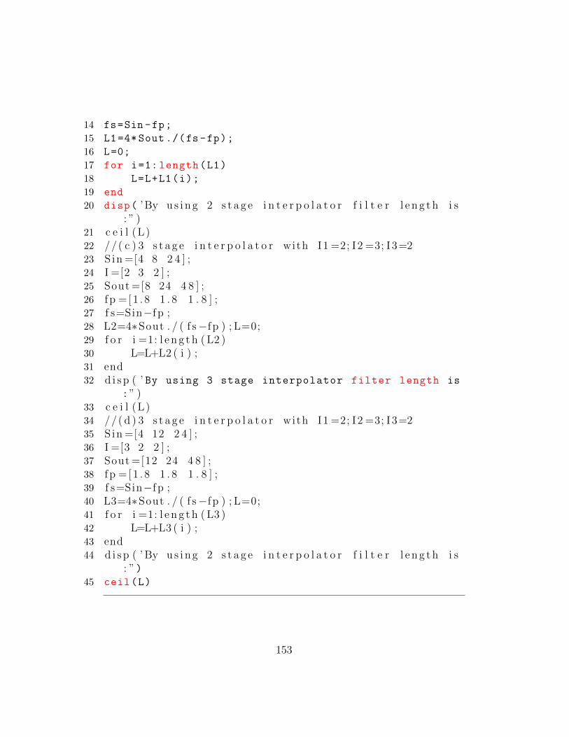
14 fs=Sin -fp;
15 L1=4* Sout ./(fs-fp);
16 L=0;
17 for i=1: length(L1)
18 L=L+L1(i);
19 end
20 disp( ’By u s i n g 2 s t a g e i n t e r p o l a t o r f i l t e r l e n g t h i s: ” )
21 c e i l (L)22 //( c ) 3 s t a g e i n t e r p o l a t o r with I1 =2; I 2 =3; I 3=223 S in =[4 8 2 4 ] ;24 I =[2 3 2 ] ;25 Sout =[8 24 4 8 ] ;26 f p = [1 . 8 1 . 8 1 . 8 ] ;27 f s=Sin−f p ;28 L2=4∗Sout . / ( f s −f p ) ; L=0;29 f o r i =1: l e n g t h ( L2 )30 L=L+L2 ( i ) ;31 end32 d i s p ( ’ By using 3 stage interpolator filter length is
:” )33 c e i l (L)34 //( d ) 3 s t a g e i n t e r p o l a t o r with I1 =2; I2 =3; I 3=235 S in =[4 12 2 4 ] ;36 I =[3 2 2 ] ;37 Sout =[12 24 4 8 ] ;38 f p = [1 . 8 1 . 8 1 . 8 ] ;39 f s=Sin−f p ;40 L3=4∗Sout . / ( f s −f p ) ; L=0;41 f o r i =1: l e n g t h ( L3 )42 L=L+L3 ( i ) ;43 end44 d i s p ( ’ By u s i n g 2 s t a g e i n t e r p o l a t o r f i l t e r l e n g t h i s
: ”)45 ceil(L)
153
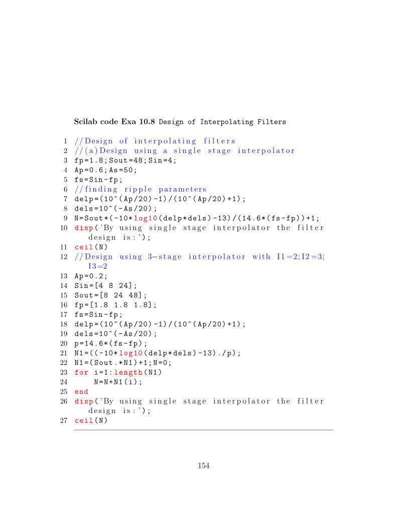
Scilab code Exa 10.8 Design of Interpolating Filters
1 // Des ign o f i n t e r p o l a t i n g f i l t e r s2 // ( a ) Des ign u s i n g a s i n g l e s t a g e i n t e r p o l a t o r3 fp=1.8; Sout =48; Sin =4;
4 Ap=0.6;As=50;
5 fs=Sin -fp;
6 // f i n d i n g r i p p l e pa ramete r s7 delp =(10^( Ap/20) -1)/(10^( Ap/20) +1);
8 dels =10^( -As/20);
9 N=Sout *( -10* log10(delp*dels) -13) /(14.6*(fs-fp))+1;
10 disp( ’By u s i n g s i n g l e s t a g e i n t e r p o l a t o r the f i l t e rd e s i g n i s : ’ );
11 ceil(N)
12 // Des ign u s i n g 3− s t a g e i n t e r p o l a t o r with I1 =2; I 2 =3;I 3=2
13 Ap=0.2;
14 Sin =[4 8 24];
15 Sout =[8 24 48];
16 fp=[1.8 1.8 1.8];
17 fs=Sin -fp;
18 delp =(10^( Ap/20) -1)/(10^( Ap/20) +1);
19 dels =10^( -As/20);
20 p=14.6*(fs-fp);
21 N1=(( -10* log10(delp*dels) -13)./p);
22 N1=(Sout.*N1)+1;N=0;
23 for i=1: length(N1)
24 N=N+N1(i);
25 end
26 disp( ’By u s i n g s i n g l e s t a g e i n t e r p o l a t o r the f i l t e rd e s i g n i s : ’ );
27 ceil(N)
154
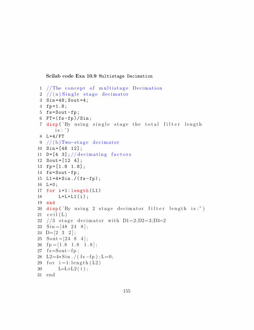
Scilab code Exa 10.9 Multistage Decimation
1 //The concep t o f m u l t i s t a g e Dec imat ion2 // ( a ) S i n g l e s t a g e dec imato r3 Sin =48; Sout =4;
4 fp=1.8;
5 fs=Sout -fp;
6 FT=(fs-fp)/Sin;
7 disp( ’By u s i n g s i n g l e s t a g e the t o t a l f i l t e r l e n g t hi s : ’ )
8 L=4/FT
9 // ( b )Two−s t a g e dec imato r10 Sin =[48 12];
11 D=[4 3]; // dec imat ing f a c t o r s12 Sout =[12 4];
13 fp=[1.8 1.8];
14 fs=Sout -fp;
15 L1=4*Sin ./(fs -fp);
16 L=0;
17 for i=1: length(L1)
18 L=L+L1(i);
19 end
20 disp( ’By u s i n g 2 s t a g e dec imato r f i l t e r l e n g t h i s : ” )21 c e i l (L)22 //3 s t a g e dec imato r with D1=2;D2=3;D3=223 S in =[48 24 8 ] ;24 D=[2 3 2 ] ;25 Sout =[24 8 4 ] ;26 f p = [1 . 8 1 . 8 1 . 8 ] ;27 f s=Sout−f p ;28 L2=4∗S in . / ( f s −f p ) ; L=0;29 f o r i =1: l e n g t h ( L2 )30 L=L+L2 ( i ) ;31 end
155
32 d i s p ( ’ By using 3 stage decimator filter length is:” )33 c e i l (L)34 //3 s t a g e dec imato r with I1 =2; I2 =3; I 3=235 S in =[48 24 1 2 ] ;36 D=[2 2 3 ] ;37 Sout =[24 12 4 ] ;38 f p = [1 . 8 1 . 8 1 . 8 ] ;39 f s=Sout−f p ;40 L3=4∗S in . / ( f s −f p ) ; L=0;41 f o r i =1: l e n g t h ( L3 )42 L=L+L3 ( i ) ;43 end44 d i s p ( ’ By u s i n g 3 s t a g e dec imato r f i l t e r l e n g t h i s : ”)45 ceil(L)
Scilab code Exa 10.10 Maximally Flat FIR filter Design
1 // Maximally f l a t FIR f i l t e r d e s i g n2 Fp=0.2;
3 Fs=0.4;
4 Fc=0.3;
5 Ft=0.2;
6 N0 =1+0.5/ Ft^2;
7 N0=ceil(N0);
8 alpha=(cos(%pi*Fc))^2;
9 k=5; Mmin =14;
10 L=Mmin -k;
11 N=2*Mmin -1;
12 disp(N, ’ Hence with t h i s l e n g t h we can ge t maximal lyf l a t FIR f i l t e r with no r i p p l e s i n passband ’ );
156
Appendix
Scilab code AP 1 Alias Frequency
1 function[F]= aliasfrequency(f,s,s1)
2 if (s>2*f) then
3 disp(” a l i a s has not occu r ed ”)4 else
5 disp(” a l i a s has oc cu r ed ”)6 end
7 F=f/s;
8 for i=1:100
9 if (abs(F) >0.5)
10 F=F-i;
11 end
12 end
13 fa=F*s1;
14 disp(fa,” f r e q u e n c y o f r e c o n s t r u c t e d s i g n a l i s ”)15 endfunction
157
Related Documents