Scilab Textbook Companion for Basic Electrical Engineering by D. C. Kulshreshtha 1 Created by Akhtar Ali Shah B.E (EXTC) Electronics Engineering AI’S Kalsekar Technical Campus New Panvel College Teacher Mrs.chaya.s Cross-Checked by Chaitanya Potti July 31, 2019 1 Funded by a grant from the National Mission on Education through ICT, http://spoken-tutorial.org/NMEICT-Intro. This Textbook Companion and Scilab codes written in it can be downloaded from the ”Textbook Companion Project” section at the website http://scilab.in

Welcome message from author
This document is posted to help you gain knowledge. Please leave a comment to let me know what you think about it! Share it to your friends and learn new things together.
Transcript

Scilab Textbook Companion forBasic Electrical Engineeringby D. C. Kulshreshtha1
Created byAkhtar Ali Shah
B.E (EXTC)Electronics Engineering
AI’S Kalsekar Technical Campus New PanvelCollege Teacher
Mrs.chaya.sCross-Checked byChaitanya Potti
July 31, 2019
1Funded by a grant from the National Mission on Education through ICT,http://spoken-tutorial.org/NMEICT-Intro. This Textbook Companion and Scilabcodes written in it can be downloaded from the ”Textbook Companion Project”section at the website http://scilab.in
Book Description
Title: Basic Electrical Engineering
Author: D. C. Kulshreshtha
Publisher: Tata McGraw Hill, New Delhi
Edition: 1
Year: 2009
ISBN: 0-07-014100-2
1
Scilab numbering policy used in this document and the relation to theabove book.
Exa Example (Solved example)
Eqn Equation (Particular equation of the above book)
AP Appendix to Example(Scilab Code that is an Appednix to a particularExample of the above book)
For example, Exa 3.51 means solved example 3.51 of this book. Sec 2.3 meansa scilab code whose theory is explained in Section 2.3 of the book.
2
Contents
List of Scilab Codes 4
2 Ohms law 5
3 Network Analysis 19
4 Network Theorems 45
5 Electromagnetism 55
6 Magnetic Circuits 62
7 Self And Mutual Inductances 66
8 DC Transients 77
9 Alternating Voltage And Current 87
10 AC Circuits 100
11 Resonance in AC Circuits 108
12 Three Phase Circuits And System 117
13 Transformers 124
3
14 Alternators And Synchronous Motors 142
15 Induction Motors 151
16 DC Machines 160
17 Fractional Horse Power Motors 178
18 Electrical Measuring Instruments 183
4
List of Scilab Codes
Exa 2.1 Resistance . . . . . . . . . . . . . . . . . . . 5Exa 2.2 Resistance . . . . . . . . . . . . . . . . . . . 6Exa 2.3 Resistance . . . . . . . . . . . . . . . . . . . 6Exa 2.4 Voltage And Current . . . . . . . . . . . . . 7Exa 2.5 Resistance . . . . . . . . . . . . . . . . . . . 8Exa 2.6 Current . . . . . . . . . . . . . . . . . . . . 9Exa 2.7 Current . . . . . . . . . . . . . . . . . . . . 10Exa 2.8 Voltage . . . . . . . . . . . . . . . . . . . . 10Exa 2.9 Resistance . . . . . . . . . . . . . . . . . . . 11Exa 2.10 Resistance . . . . . . . . . . . . . . . . . . . 12Exa 2.11 Resistance . . . . . . . . . . . . . . . . . . . 13Exa 2.12 Resistance . . . . . . . . . . . . . . . . . . . 13Exa 2.13 Cost . . . . . . . . . . . . . . . . . . . . . . 14Exa 2.14 Rating . . . . . . . . . . . . . . . . . . . . . 15Exa 2.15 Resistance . . . . . . . . . . . . . . . . . . . 15Exa 2.16 Resistance . . . . . . . . . . . . . . . . . . . 16Exa 2.17 Resistance . . . . . . . . . . . . . . . . . . . 17Exa 2.18 Temperature . . . . . . . . . . . . . . . . . 17Exa 3.1 capacitor . . . . . . . . . . . . . . . . . . . 19Exa 3.2 Inductor . . . . . . . . . . . . . . . . . . . . 20Exa 3.3 Inductor . . . . . . . . . . . . . . . . . . . . 21Exa 3.4 Voltage . . . . . . . . . . . . . . . . . . . . 22Exa 3.5 Voltage . . . . . . . . . . . . . . . . . . . . 23Exa 3.6 Voltage And Energy . . . . . . . . . . . . . 24Exa 3.7 Capacitor . . . . . . . . . . . . . . . . . . . 25Exa 3.8 Voltage And Current . . . . . . . . . . . . . 26Exa 3.9 Voltage And Power . . . . . . . . . . . . . . 28Exa 3.10 Current . . . . . . . . . . . . . . . . . . . . 29
5
Exa 3.13 Current And Power . . . . . . . . . . . . . . 30Exa 3.14 Voltage . . . . . . . . . . . . . . . . . . . . 31Exa 3.15 Voltage . . . . . . . . . . . . . . . . . . . . 31Exa 3.16 Current . . . . . . . . . . . . . . . . . . . . 32Exa 3.17 Resistance . . . . . . . . . . . . . . . . . . . 34Exa 3.18 Current . . . . . . . . . . . . . . . . . . . . 35Exa 3.19 Voltage . . . . . . . . . . . . . . . . . . . . 35Exa 3.20 Current . . . . . . . . . . . . . . . . . . . . 36Exa 3.21 Current . . . . . . . . . . . . . . . . . . . . 37Exa 3.22 Voltage . . . . . . . . . . . . . . . . . . . . 38Exa 3.23 Current . . . . . . . . . . . . . . . . . . . . 39Exa 3.24 Current . . . . . . . . . . . . . . . . . . . . 40Exa 3.25 Voltage . . . . . . . . . . . . . . . . . . . . 41Exa 2.26 Current . . . . . . . . . . . . . . . . . . . . 42Exa 2.27 Current . . . . . . . . . . . . . . . . . . . . 43Exa 4.1 Current . . . . . . . . . . . . . . . . . . . . 45Exa 4.2 Current . . . . . . . . . . . . . . . . . . . . 46Exa 4.3 Voltage . . . . . . . . . . . . . . . . . . . . 47Exa 4.4 Current . . . . . . . . . . . . . . . . . . . . 48Exa 4.5 Voltage . . . . . . . . . . . . . . . . . . . . 49Exa 4.6 Voltage . . . . . . . . . . . . . . . . . . . . 50Exa 4.7 Current . . . . . . . . . . . . . . . . . . . . 50Exa 4.8 Power . . . . . . . . . . . . . . . . . . . . . 51Exa 4.9 Power . . . . . . . . . . . . . . . . . . . . . 52Exa 4.10 Voltage And Power . . . . . . . . . . . . . . 53Exa 4.11 Current And Resistance . . . . . . . . . . . 54Exa 5.1 Current . . . . . . . . . . . . . . . . . . . . 55Exa 5.2 Megnetic Field Strength . . . . . . . . . . . 55Exa 5.3 Force . . . . . . . . . . . . . . . . . . . . . . 56Exa 5.4 Force . . . . . . . . . . . . . . . . . . . . . . 57Exa 5.5 Voltage . . . . . . . . . . . . . . . . . . . . 58Exa 5.6 Voltage . . . . . . . . . . . . . . . . . . . . 58Exa 5.7 Voltage . . . . . . . . . . . . . . . . . . . . 59Exa 5.8 Voltage Time And Force . . . . . . . . . . . 60Exa 6.1 Megnetic Field Strength And Flux . . . . . 62Exa 6.2 Megnetomotive Force . . . . . . . . . . . . . 63Exa 6.3 Reluctance And Current . . . . . . . . . . . 63Exa 6.4 Current . . . . . . . . . . . . . . . . . . . . 64
6
Exa 7.1 Voltage . . . . . . . . . . . . . . . . . . . . 66Exa 7.2 Inductor And Voltage . . . . . . . . . . . . 66Exa 7.3 Inductor And Voltage . . . . . . . . . . . . 67Exa 7.4 Inductor And Energy . . . . . . . . . . . . . 68Exa 7.5 Megnetic Field Strength And Voltage . . . . 68Exa 7.6 Voltage . . . . . . . . . . . . . . . . . . . . 69Exa 7.7 Inductor And Voltage . . . . . . . . . . . . 70Exa 7.8 Inductor . . . . . . . . . . . . . . . . . . . . 71Exa 7.9 Inductor . . . . . . . . . . . . . . . . . . . . 72Exa 7.10 Inductor . . . . . . . . . . . . . . . . . . . . 73Exa 7.11 Inductor . . . . . . . . . . . . . . . . . . . . 74Exa 7.12 Inductor . . . . . . . . . . . . . . . . . . . . 75Exa 8.1 Voltage . . . . . . . . . . . . . . . . . . . . 77Exa 8.2 Current And Power . . . . . . . . . . . . . . 78Exa 8.3 Current And Time . . . . . . . . . . . . . . 79Exa 8.4 Current . . . . . . . . . . . . . . . . . . . . 80Exa 8.5 Current . . . . . . . . . . . . . . . . . . . . 81Exa 8.6 Voltage And Current . . . . . . . . . . . . . 83Exa 8.7 Voltage And Current . . . . . . . . . . . . . 84Exa 8.8 Current . . . . . . . . . . . . . . . . . . . . 85Exa 9.1 Voltage And Angle . . . . . . . . . . . . . . 87Exa 9.2 Voltage Time And Frequency . . . . . . . . 87Exa 9.3 Voltage . . . . . . . . . . . . . . . . . . . . 88Exa 9.4 Current And Time . . . . . . . . . . . . . . 89Exa 9.5 Time . . . . . . . . . . . . . . . . . . . . . . 90Exa 9.6 Power . . . . . . . . . . . . . . . . . . . . . 91Exa 9.7 Current . . . . . . . . . . . . . . . . . . . . 92Exa 9.8 Current . . . . . . . . . . . . . . . . . . . . 92Exa 9.9 Current . . . . . . . . . . . . . . . . . . . . 93Exa 9.10 Current . . . . . . . . . . . . . . . . . . . . 94Exa 9.11 Voltage . . . . . . . . . . . . . . . . . . . . 94Exa 9.12 Voltage . . . . . . . . . . . . . . . . . . . . 95Exa 9.13 Current And Power Factor . . . . . . . . . . 96Exa 9.14 Voltage And Power Factor . . . . . . . . . . 97Exa 9.15 Power And Power Factor . . . . . . . . . . . 98Exa 10.1 Current Power And Power Factor . . . . . . 100Exa 10.2 Current Power And Power Factor . . . . . . 101Exa 10.3 Resistance Voltage And Power . . . . . . . 102
7
Exa 10.4 Resistance Power And Power Factor . . . . 103Exa 10.5 Reluctance And Inductor . . . . . . . . . . . 104Exa 10.6 Resistance And Capacitor . . . . . . . . . . 105Exa 10.7 Resistance Power And Power Factor . . . . 106Exa 11.1 Frequence And Voltage . . . . . . . . . . . . 108Exa 11.2 Capacitor Voltage And Q FActor . . . . . . 109Exa 11.3 Inductor Current And Voltage . . . . . . . . 110Exa 11.4 Capacitor Current And Enegy . . . . . . . . 111Exa 11.5 Frequence And Q Factor . . . . . . . . . . . 112Exa 11.6 Frequence . . . . . . . . . . . . . . . . . . . 113Exa 11.7 Resistance Current And Capacitor . . . . . 114Exa 11.8 Frequence And Q Factor . . . . . . . . . . . 115Exa 12.1 Current . . . . . . . . . . . . . . . . . . . . 117Exa 12.2 Current . . . . . . . . . . . . . . . . . . . . 118Exa 12.3 Current . . . . . . . . . . . . . . . . . . . . 119Exa 12.4 Current Power And Power Factor . . . . . . 120Exa 12.5 Power And Power Factor . . . . . . . . . . . 121Exa 12.6 Current Power And Power Factor . . . . . . 122Exa 13.1 Megnetic Flux And Voltage . . . . . . . . . 124Exa 13.2 Flux Density Current And Voltage . . . . . 125Exa 13.3 Turns Ratio . . . . . . . . . . . . . . . . . . 126Exa 13.4 Current . . . . . . . . . . . . . . . . . . . . 126Exa 13.5 Power . . . . . . . . . . . . . . . . . . . . . 127Exa 13.6 Turns . . . . . . . . . . . . . . . . . . . . . 128Exa 13.7 Current And Power Factor . . . . . . . . . . 129Exa 13.8 Power . . . . . . . . . . . . . . . . . . . . . 130Exa 13.9 Current And Power Factor . . . . . . . . . . 131Exa 13.10 Resistance And Power . . . . . . . . . . . . 132Exa 13.11 Regulation . . . . . . . . . . . . . . . . . . . 134Exa 13.12 Efficiency And Power . . . . . . . . . . . . . 135Exa 13.13 Efficiency . . . . . . . . . . . . . . . . . . . 137Exa 13.14 Power . . . . . . . . . . . . . . . . . . . . . 138Exa 13.15 Voltage . . . . . . . . . . . . . . . . . . . . 139Exa 13.16 Current And Resistance . . . . . . . . . . . 140Exa 14.1 Speed . . . . . . . . . . . . . . . . . . . . . 142Exa 14.2 Distribution Factor . . . . . . . . . . . . . . 143Exa 14.3 Speed Emf And Voltage . . . . . . . . . . . 143Exa 14.4 Voltage Regulation . . . . . . . . . . . . . . 144
8
Exa 14.5 Voltage Regulation . . . . . . . . . . . . . . 146Exa 14.6 Emf And Angle . . . . . . . . . . . . . . . . 147Exa 14.7 Emf . . . . . . . . . . . . . . . . . . . . . . 148Exa 14.8 Emf . . . . . . . . . . . . . . . . . . . . . . 149Exa 14.9 Current Power And Torque . . . . . . . . . 150Exa 15.1 Speed And Frequency . . . . . . . . . . . . 151Exa 15.2 Speed And Frequency . . . . . . . . . . . . 152Exa 15.3 Speed . . . . . . . . . . . . . . . . . . . . . 153Exa 15.4 Speed And Frequency . . . . . . . . . . . . 153Exa 15.5 Current . . . . . . . . . . . . . . . . . . . . 154Exa 15.6 Power And Speed . . . . . . . . . . . . . . . 156Exa 15.7 Current Power And Speed . . . . . . . . . . 157Exa 15.8 Resistance . . . . . . . . . . . . . . . . . . . 159Exa 16.1 Voltage Current And Power . . . . . . . . . 160Exa 16.2 Emf . . . . . . . . . . . . . . . . . . . . . . 161Exa 16.3 Emf . . . . . . . . . . . . . . . . . . . . . . 162Exa 16.4 Speed And increase in flux . . . . . . . . . . 162Exa 16.5 Voltage . . . . . . . . . . . . . . . . . . . . 163Exa 16.6 Voltage And Current . . . . . . . . . . . . . 164Exa 16.7 Emf . . . . . . . . . . . . . . . . . . . . . . 165Exa 16.8 Voltage Efficiency And Power . . . . . . . . 166Exa 16.9 Current And Resistance . . . . . . . . . . . 167Exa 16.10 Turns . . . . . . . . . . . . . . . . . . . . . 168Exa 16.11 Voltage . . . . . . . . . . . . . . . . . . . . 169Exa 16.12 Speed . . . . . . . . . . . . . . . . . . . . . 169Exa 16.13 Speed . . . . . . . . . . . . . . . . . . . . . 170Exa 16.14 Speed And Torque . . . . . . . . . . . . . . 171Exa 16.15 Power . . . . . . . . . . . . . . . . . . . . . 172Exa 16.16 Speed . . . . . . . . . . . . . . . . . . . . . 172Exa 16.17 Current . . . . . . . . . . . . . . . . . . . . 173Exa 16.18 Speed And Torque . . . . . . . . . . . . . . 174Exa 16.19 Resistance . . . . . . . . . . . . . . . . . . . 175Exa 16.20 Speed . . . . . . . . . . . . . . . . . . . . . 176Exa 17.1 Slip And Efficiency . . . . . . . . . . . . . . 178Exa 17.2 Current Phase Angle And Power Factor . . 179Exa 17.3 Capacitor . . . . . . . . . . . . . . . . . . . 180Exa 17.4 Revolution Steps And Speed . . . . . . . . . 181Exa 17.5 No of Rotors And Stators . . . . . . . . . . 181
9
Exa 17.6 No of Rotors And Stators Theeth . . . . . . 182Exa 18.1 Torque . . . . . . . . . . . . . . . . . . . . . 183Exa 18.2 Resistance . . . . . . . . . . . . . . . . . . . 184Exa 18.4 Resistance . . . . . . . . . . . . . . . . . . . 184Exa 18.5 Resistance And Multiplying Factor . . . . . 185Exa 18.6 Voltage And Error . . . . . . . . . . . . . . 186Exa 18.7 Angle of Deflection . . . . . . . . . . . . . . 187Exa 18.8 Deflection in the Torque . . . . . . . . . . . 187Exa 18.9 Angle of Deflection . . . . . . . . . . . . . . 188Exa 18.10 Current . . . . . . . . . . . . . . . . . . . . 189
10
Chapter 2
Ohms law
Scilab code Exa 2.1 Resistance
1
2
3 // Example 2 . 14
5 a1=%pi *2^2/4; // R e l a t i v e a r ea o f wire−A6 a2=%pi *1/4; // R e l a t i v e a r ea o f wire−B7 l1=1; // R e l a t i v e l e n g h t o f wire−B8 l2=4; // R e l a t i v e l e n g h t o f wire−B9 R1=5; // R e s i s t a n c e o f w i r e10 r=(l2/a2)/(l1/a1);
11 disp( ’ The r a t i o o f r e s i s t a n c e s (R2/R1) = ’ +string(r)+ ’ ohm ’ );
12 R2=r*R1;
13 disp( ’ R e s i s t a n c e (R2) = ’ +string(R2)+ ’ ohm ’ );14
15
16
17
18
19 // p 16 2 . 1
11
Scilab code Exa 2.2 Resistance
1
2 // Example 2 . 23
4
5 a1=%pi *3/4; // R e l a t i v e a r ea o f wire−A6 a2=%pi *1/4; // R e l a t i v e a r ea o f wire−B7 l1=1; // R e l a t i v e l e n g h t o f wire−A8 l2=3; // R e l a t i v e l e n g h t o f wire−B9 R1=10; // R e s i s t a n c e o f w i r e
10 r=(l2/a2)/(l1/a1);
11 disp( ’ The r a t i o o f r e s i s t a n c e s (R2/R1) = ’ +string(r)+ ’ ohm ’ );
12 R2=r*R1;
13 disp( ’ R e s i s t a n c e (R2) = ’ +string(R2)+ ’ ohm ’ );14
15
16
17
18
19
20
21 // p 16 2 . 2
Scilab code Exa 2.3 Resistance
1
2 // Example 2 . 33
4 // Rp=(4+4) | | ( 8 + 4 )5
12
6 Rp =(8*12) /(8+12); // By Vo l tage d i v i d e r r u l e7 disp( ’ v o l t a g e Acros s Foue r e s i s r a n c e = ’ +string(Rp)
+ ’ Ohm ’ );8
9
10
11
12
13 // p 20 2 . 3
Scilab code Exa 2.4 Voltage And Current
1
2
3 // Example 2 . 44
5 v=8.8*{2/(2+2.4) }; // by v o l t a g e d i v i d e r r u l e6 disp( ’ Anknown Vo l tage a c r o s s the R1 = ’ +string(v)+ ’
v o l t ’ );7
8 v1 =8.8*{2.4/(2+2.4) }; // by v o l t a g e d i v i d e r r u l e9 disp( ’ Anknown Vo l tage a c r o s s the R1 = ’ +string(v1)+
’ v o l t ’ );10 i=4.8/4; // I=V/R11 disp( ’ Anknown Current I1 = ’ +string(i)+ ’ Amp ’ );12 i1 =4.8/6; // I=V/R13 disp( ’ Anknown Current I2 = ’ +string(i1)+ ’ Amp ’ );14
15
16
17
18
19 // p 20 2 . 4
13
Scilab code Exa 2.5 Resistance
1
2 // Example 2 . 53
4 // From the diagram 2 . 1 45
6 rp =(1/20) +(1/10) +(1/20); // P a r a l l e lr e s i s t a n c e
7 Rp=1/rp; // The r e s i s t a n c e Rp8 Rs=15; // S e r i e s r e s i s t a n c e9 Rab=Rs+Rp; // E f f e c t i v e
r e s i s t a n c e between A & B10 disp( ’ ( a ) E f f e c t i v e r e s i s t a n c e between A & B f o r
diagram ( a ) = ’ +string(Rab)+ ’ Ohms ’ );11
12 // f o r diagram ( b ) network above l i n e ABi . e R1=[(R+R) | |R]+R
13 R1=5/3; // R e s i s t a n c e o fnetwork
14 R2=R1; // The l owe r pa r t i sa l s o same as R1
15 R12 =5/6; // Combination o f R1& R2
16 Rab1=(R12*1)/(R12+1); // E f f e c t i v er e s i s t a n c e between A & B f o r diagram ( b )
17 disp( ’ ( b ) E f f e c t i v e r e s i s t a n c e between A & B f o rdiagram ( b ) = ’ +string(Rab1)+ ’ R ’ );
18
19 // f o r diagram ( c )20 r1 =(3*6) /(3+6); // P a r a l l e l
combinat i on o f 3 & 6 Ohms R e s i s t a n c e21 Ri=r1+18; // s e r i e s o f r1 & 18
Ohms R e s i s t a n c e
14
22 rab =(20*20) /(20+20); // P a r a l l e lcombinatu ion o f Ri & 20 Ohms R e s i s t a n c e
23 Rab2=rab+5; // s e r i e s o f rab & 2Ohms R e s i s t a n c e
24 disp( ’ ( c ) E f f e c t i v e r e s i s t a n c e between A & B f o rdiagram ( c ) = ’ +string(Rab2)+ ’ Ohms ’ );
25
26
27
28
29 // p 23 2 . 5
Scilab code Exa 2.6 Current
1
2 // Example 2 . 63
4 d=(1/12) +(1/20) +(1/30);
5 Reff =2+(1/d); // E f f e c t i v e R e s i s r e n c e6 v=100;
7 I=v/Reff;
8 // ( but 12 i 1= 20 i 2= 30 i 3 )9 // i 2= 12/20 ∗ i 1 & i 3= 12/30 ∗ i 1
10 // but 10= i 1+i 2+i 311 // 0 . 6 i 1 +0.4 i 1+i 1 =10 i . e i 1 =512 i1=5;
13 disp( ’ Current o f I 1 i f = ’ +string(i1)+ ’ Amp ’ );14 i2=0.6*i1;
15 disp( ’ Current o f I 2 i f = ’ +string(i2)+ ’ Amp ’ );16 i3=0.4*i1;
17 disp( ’ Current o f I 3 i f = ’ +string(i3)+ ’ Amp ’ );18
19
20
21 // p 24 2 . 6
15
Scilab code Exa 2.7 Current
1
2 // Example 2 . 73
4 // p=i 1 ˆ2∗Rl i . e i 1=p/ Rl5
6 Rl=5; // Load r e s i s t a n c e7 p=20; // Power8 i1=p/Rl;
9 // i 1= i ∗ (R/R+Rl ) i . e i= i 1 ∗ (R+Rl ) /R10 i=2*(10+5) /10;
11 disp( ’ Supply Current i s = ’ +string(i)+ ’ Amp ’ );12
13
14 // p 25 2 . 7
Scilab code Exa 2.8 Voltage
1
2 // Example 2 . 83
4 v=120; // Supply v o l t a g e5 p=60; // Power6 R=v^2/p; // R e s i s t a n c e7
8 // the combinat ion R o f bulb B & C i s Rbc=240/2 i . e Rbc=120
9 // vb=vc10
11 Rbc =240/2; // R o f each bulb
16

12 k=240+120;
13 vc=Rbc *(120/k); // v o l t a c r o s s Vc & Vb {u s i n g Vol t D i v i d e r Rule }
14 va=120 -40; // v o l t a c r o s s Va15 disp( ’ the Vo l tage a c r o s s bulb A & B = ’ +string(vc)+
’ Vo l t ’ );16 disp( ’ the Vo l tage a c r o s s bulb C = ’ +string(va)+ ’
Vo l t ’ );17 vb=40;
18 p=(va)^2/240+( vb)^2/240+( vc)^2/240; // p=pa+pb+pc t o t a l power
19
20 disp( ’ To ta l e Power D i s s i p a t e d i s = ’ +string(p)+ ’Watt ’ );
21
22
23 // p 25 2 . 8
Scilab code Exa 2.9 Resistance
1
2 // Example 2 . 93
4 // From the diagram 2 . 1 85 // Minimum v a l u e o f Req i s o b t a i n e d i f R
=06 // Maximum v a l u e o f Req i s o b t a i n e d i f R
= Open ckt7
8 R1=30; // Given the v a l u e o f R1& R1+R2= 75
9 R2=75-R1; // The v a l u e o f R210 disp( ’ The v a l u e o f R1 i s = ’ +string(R1)+ ’ Ohms ’ );11 disp( ’ The v a l u e o f R2 i s = ’ +string(R2)+ ’ Ohms ’ );12
17

13 // From the diagram 2 . 1 914
15 Req= (30+75) /2; // Requ i red v a l u e o f Reqi s Req= (30+75) /2
16 Rp=Req -R1; // Hance the p a r a l l e lcombinat i on o f R2 & R
17 disp( ’ The v a l u e o f Rp i s = ’ +string(Rp)+ ’ Ohms ’ );18 disp( ’ The v a l u e o f Rp i s e x a c t l y h a l f o f R2= 45 ,
hance the v a l u e o f R shou ld be ’ +string(R2)+ ’Ohms ’ );
19
20
21
22
23 // p 26 2 . 9
Scilab code Exa 2.10 Resistance
1
2 // Example 2 . 1 03
4 // Rx=R+(R | | 2 Rx)5 // i . e 2∗Rxˆ2−3R Rx−Rˆ2 =06 R=1;
7 Rx={3*R+sqrt (9*R*R+8*R*R)}/4; // Using Roots o fc o d r a t i c Equat ion
8
9 disp( ’ E q u i v a l e n t R i s = ’ +string(Rx)+ ’ R ’ );10
11
12
13
14
15 // p 26 2 . 1 0
18

Scilab code Exa 2.11 Resistance
1
2
3 // Example 2 . 1 14
5 // To conve t Pi− S e c t i o n i n to T−S e c t i o n .
6 // We have to Find Ra , Rb & Rc f o r T−S e c t i o n
7 R2=9; // R e s i s t a n c e o f 9 Ohms8 R3=6; // R e s i s t a n c e o f 6 Ohms9 R1=3; // R e s i s t a n c e o f 3 Ohms
10
11 Ra=(R2*R3)/(R1+R2+R3);
12 disp( ’ Value o f Ra i s = ’ +string(Ra)+ ’ Ohm ’ );13 Rb=(R1*R3)/(R1+R2+R3);
14 disp( ’ Value o f Rc i s = ’ +string(Rb)+ ’ Ohm ’ );15 Rc=(R2*R1)/(R1+R2+R3);
16 disp( ’ Value o f Rc i s = ’ +string(Rc)+ ’ Ohm ’ );17
18
19
20 // p 26 2 . 1 1
Scilab code Exa 2.12 Resistance
1
2
3 // Example 2 . 1 24
5 Reff= 100/10; // E f f e c t i v e R
19
6
7 // P=v ˆ2/R i . e Power o f c o i l8 v=100;
9 R=600;
10 R1=v^2/R;
11 // 2 C o i l a r e connec t edp a r a l l e l
12 R2=(R1*10)/(R1 -10); // Using p a r a l l e l Rfo rmu la
13
14 disp( ’ R e s i s t a n c e o f each c o i l = ’ +string(R2)+ ’ Ohm ’);
15
16
17
18 // p 27 2 . 1 2
Scilab code Exa 2.13 Cost
1
2
3
4 // Example 2 . 1 35
6 v=115; // Vo l tage7 i=12; // c u r r e n t8 t=6; // Time Requ i red9 w=v*i*t; // Energy10 Rate =2.50;
11 Cost=w*Rate;
12 disp( ’ c o s t o f b o i l e r Operat i on i s = ’ +string(Cost/1000)+ ’ Rs/kwh ’ );
13
14
15
20
16
17
18 // p 27 2 . 1 3
Scilab code Exa 2.14 Rating
1
2
3
4 // Example 2 . 1 45
6 v=240;
7 p=1000; // t o a s t e r r e t e d at 1000 w8 R=v^2/p; // r e s i s t a n c r a r i n g9 Imax=p/v; // Current r a t i n g
10 v1=220;
11 I=v1/R; // Current at 220 v12 p1=v1*I;
13 disp( ’ Power r a t i n g i s = ’ +string(p1)+ ’ Watt ’ );14 disp( ’ t h e r e f o r the Power r a t i n g i s l e s s then
o r i g i n a l power . ’ );15
16
17
18
19
20 // p 28 2 . 1 4
Scilab code Exa 2.15 Resistance
1
2 // Example 2 . 1 53
21
4 // To f i n d the Value o f R e s i s t e r5 // We Sghould know About Colour Code6
7 Y=4; // Yelow c o l o u r8 V=7; // V i o l e t c o l o u r9 O=10^3; // Orenge c o l o u r
10 r=(10*Y+V)*O;
11 R=r*(5/100);
12 disp( ’ The v a l u e o f R e s i s t a n c e i s = ’ +string(R)+ ’ohm ’ );
13
14
15
16
17 // p 30 2 . 1 5
Scilab code Exa 2.16 Resistance
1
2
3 // Example 2 . 1 64
5 // To f i n d the Value o f R e s i s t e r6 // We Sghould know About Colour
Code7 Gr=8; // Gray c o l o u r8 B=6; // Blue c o l o u r9 G=10^ -1; // Gold c o l o u r
10 r=(10* Gr+B)*G;
11 R=r*(5/100);
12 disp( ’ The v a l u e o f R e s i s t a n c e i s = ’ +string(R)+ ’ohm ’ );
13
14
15
22
16
17 // p 30 2 . 1 6
Scilab code Exa 2.17 Resistance
1
2
3 // Example 2 . 1 74
5 R1=126; // R e s i s t a n c e o f 126 Ohms6 T1=20; // t empera tu r e at 126 ohms r e s i s t o r7 T2=-35; // Temperature ( −35 D ig r e e )8 ao =0.00426;
9 // By u s i n g Temprerature Formula i . eR1/(1+aoT1 ) =R2/(1+aoT2 )
10 z=(1+ao*T2)/(1+ao*T1);
11 R2=R1*z;
12 disp( ’ R e s i s t a n c e o f the l i n e ( at T=−35) = ’ +string(R2)+ ’ Ohm ’ );
13
14
15
16
17
18 // p 31 2 . 1 7
Scilab code Exa 2.18 Temperature
1
2
3 // Example 2 . 1 84
5 R1 =3.42; // R e s i s t a n c e o f 3 . 4 2 Ohms
23
6 T1=20; // t empera tu r e at 3 . 4 2 ohms r e s i s t o r7 R2 =4.22; // R e s i s t a n c e R28 ao =0.00426;
9
10 // By u s i n g Temprerature Formula ==> i . e R1/(1+aoT1 ) =R2/(1+aoT2 )
11
12 z=(R2/R1)*(1+ao*T1);
13 T2=(z-1)/ao;
14 T=T2 -T1; // Temperature R i s e15 disp( ’ The Temperature R i s e i s = ’ +string(T)+ ’
D i g r e e C e l s i u s ’ );16
17
18
19
20
21 // p 32 2 . 1 8
24
Chapter 3
Network Analysis
Scilab code Exa 3.1 capacitor
1
2
3 // Examle 3 . 14
5 A=0.113; // Area o f p a r a l l e l p l a t e6 eo =8.854*10^ -12; // P e r m i t t i v i t y o f f r e e
space7 er=10; // R e l a t i v e P e r m i t t i v i t y8 d=0.1*10^ -3; // D i s t a n c e between 2
P l a t e9 C=(eo*er*A)/d; // The v a l u e o f c a p a c i t o r
Using case−110 disp( ’ The v a l u e o f c a p a c i t o r Using case−1 = ’ +
string(C*1000000)+ ’ uF ’ );11
12 w=0.05; // Energy s t o r e d13 v=100; // Vo l tage14 C1=(2*w)/v^2; // The v a l u e o f c a p a c i t o r
Using case−215 disp( ’ The v a l u e o f c a p a c i t o r Using case−2 = ’ +
string(C1 *1000000)+ ’ uF ’ );
25

16
17 i=5*10^ -3; // Current18 dv=100; // I n c r e a s e i v v o l t a g e19 dt=0.1; // Time r e q u i r e d20 C2=i/(dv/dt); // The v a l u e o f c a p a c i t o r
Using case−321 disp( ’ The v a l u e o f c a p a c i t o r Using case−3 = ’ +
string(C2 *1000000)+ ’ uF ’ );22
23
24
25
26
27
28 // p 53 3 . 1
Scilab code Exa 3.2 Inductor
1
2
3 // Examle 3 . 24
5 w=0.2; // Energy s t o r e d6 i=0.2; // Current7 L1=(2*w)/i^2; // The v a l u e o f
I n d u c t o r Using case−18 disp( ’ The v a l u e o f I n d u c t o r Using case−1 = ’ +string
(L1)+ ’ H ’ );9
10 v=10; // Vo l tage11 di1 =0.1; // I n c r e a s e c u r r e n t12 dt1 =0.2; // Time r e q u i r e d13 L2=v/(di1/dt1); // The v a l u e o f
I n d u c t o r Using case−214 disp( ’ The v a l u e o f I n d u c t o r Using case−2 = ’ +string
26

(L2)+ ’ H ’ );15
16
17 p=2.5; // Power18 di2 =0.1; // I n c r e a s e c u r r e n t19 dt2 =0.5; // Time r e q u i r e d20 L3=p/(di2*dt2); // The v a l u e o f
I n d u c t o r Using case−321 disp( ’ The v a l u e o f I n d u c t o r Using case−3 = ’ +string
(L3)+ ’ H ’ );22
23
24
25
26 // p 54 3 . 2
Scilab code Exa 3.3 Inductor
1
2 // Examle 3 . 33
4 // Given L1= 2L25 // From the Diagram Leq=
0.5+ ( L1∗L2 ) /( L1+L2 )6 // t h e r e f o r ( L1∗L2 ) /( L1+
L2 )= 0 . 2 , ( where Leq=0 . 7 )
7 // i . e (2∗L2∗L2 ) /3L2= 0 . 2 ;8 // i t means L2= 0 . 3 H9
10 L2=0.3; // Value o f I n d u c t o r 111 L1=2*L2; // Value o f I n d u c t o r 212 disp( ’ Value o f I n d u c t o r s a r e L1= ’ +string(L1)+ ’ H
& L2= ’ +string(L2)+ ’ H ’ );13
27

14
15
16
17
18
19 // p 55 3 . 3
Scilab code Exa 3.4 Voltage
1
2 // Examle 3 . 43
4 C1 =0.05; // C a pa c i t o r1 ( i n Micro )
5 C2=0.1; // C a pa c i t o r2 ( i n Micro )
6 C3=0.2; // C a pa c i t o r3 ( i n Micro )
7 C4 =0.05; // C a pa c i t o r4 ( i n Micro )
8 C=(1/C1)+(1/C2)+(1/C3)+(1/C4); // Add i t i ono f c a p a c i t o r s
9 Cs=1/C; // E q u i v a l e n tc a p a c i t o r
10 disp( ’ E q u i v a l e n t c a p a c i t o r = ’ +string(Cs)+ ’ uF ’ );11
12 V=220; // Supplyv o l t a g e
13 Q=Cs*V; // Charget r a n s f e r
14 V1=Q/C1; // Vo l tagedrop a c r o s s c a p a c i t o r 1
15 disp( ’ Vo l tage drop a c r o s s c a p a c i t o r 1 = ’ +string(V1)+ ’ Vo l t ’ );
16
28
17 V2=Q/C2; // Vo l tagedrop a c r o s s c a p a c i t o r 2
18 disp( ’ Vo l tage drop a c r o s s c a p a c i t o r 2 = ’ +string(V2)+ ’ Vo l t ’ );
19
20 V3=Q/C3; // Vo l tagedrop a c r o s s c a p a c i t o r 3
21 disp( ’ Vo l tage drop a c r o s s c a p a c i t o r 3 = ’ +string(V3)+ ’ Vo l t ’ );
22
23 V4=Q/C4; // Vo l tagedrop a c r o s s c a p a c i t o r 4
24 disp( ’ Vo l tage drop a c r o s s c a p a c i t o r 4 = ’ +string(V4)+ ’ Vo l t ’ );
25
26
27
28
29 // p 55 3 . 4
Scilab code Exa 3.5 Voltage
1
2 // Examle 3 . 53
4 C1=2*10^ -6; // Value o f c a p a c i t o r −15 C2=10*10^ -6; // Value o f c a p a c i t o r −26 Q1 =400*10^ -6; // Charge o f c a p a c i t o r −17 Q2 =200*10^ -6; // Charge o f c a p a c i t o r −28 Q=Q1+Q2; // Tota l Charge o f
c a p a c i t o r s9 C=C1+C2; // E q u i v a l e n t s s c a p a c i t o r10 V=Q/C; // Vo l tage a c r o s s the
c a p a c i t o r11 disp( ’ Vo l tage a c r o s s the c a p a c i t o r = ’ +string(V)+ ’
29
Volt ’ );12
13
14
15
16
17
18 // p 55 3 . 5
Scilab code Exa 3.6 Voltage And Energy
1
2 // Examle 3 . 63
4 C1=2*10^ -6; // C a p ac i t o r1
5 C2=8*10^ -6; // C a p ac i t o r2
6 C=(C1*C2)/(C1+C2); //E q u i v a l e n t s s c a p a c i t o r
7 V=300; // Supplyv o l t a g e
8 Q=C*V; // Charge oneach c a p a c i t o r
9 disp( ’ ( a ) Charge on each c a p a c i t o r = ’ +string(Q*1000000)+ ’ uC ’ );
10
11 V1=Q/C1; // Vo l tagedrop a c r o s s c a p a c i t o r 1
12 disp( ’ ( b ) . 1 Vo l tage drop a c r o s s c a p a c i t o r 1 = ’ +string(V1)+ ’ Vo l t ’ );
13
14 V2=Q/C2; // Vo l tagedrop a c r o s s c a p a c i t o r 2
15 disp( ’ ( b ) . 2 Vo l tage drop a c r o s s c a p a c i t o r 2 = ’ +
30

string(V2)+ ’ Vo l t ’ );16
17 V1=240;
18 w1=0.5*C1*V1^2; // Energys t o r e d i n c a p a c i t o r −1
19 disp( ’ ( c ) . 1 Energy s t o r e d i n c a p a c i t o r −1 = ’ +string(w1 *1000)+ ’ mJ ’ );
20
21 V2=60;
22 w2=0.5*C2*V2^2; // Energys t o r e d i n c a p a c i t o r −2
23 disp( ’ ( c ) . 2 Energy s t o r e d i n c a p a c i t o r −2 = ’ +string(w2 *1000)+ ’ mJ ’ );
24
25
26
27
28
29
30 // p 56 3 . 6
Scilab code Exa 3.7 Capacitor
1
2
3 // Examle 3 . 74
5 // Given tha t Ceq= 1 uFbetween A & B
6 // By r e d u c i n g thec i r c u i t w i l l g e t 2c a p a c i t o r .
7 // tha t i s C & C13= 32/9uF
8 // t h e r e f o r ( 1 / 1 )= 1/C+
31
9/329 // Hance 1/C= 1−9/3210 C=1/{1 -(9/32) }; // Value o f Capac i to r−C11 disp( ’ Value o f C a p a c i t o r C = ’ +string(C)+ ’ uF ’ );12
13
14
15
16
17
18
19 // p 56 3 . 7
Scilab code Exa 3.8 Voltage And Current
1
2 // Examle 3 . 83
4 // f o r the extreme v a l u eo f Rl v o l t a g e ( Vl ) &Current ( I l )
5 E=3; // Supply v o l t a g e6 Ri=1; // I /p R e s i s t a n c e7 Rl1 =100; // Minimum load
r e s i s t a n c e8 Il1=E/(Rl1+Ri); // Current at minimum
load Rl19 Vl1=E-(Il1*Ri); // Vo l tage at minimum
load Rl110
11 Rl2 =1000; // Maximum loadr e s i s t a n c e
12 Il2=E/(Rl2+Ri); // Current at maximumload Rl2
13 Vl2=E-(Il2*Ri); // Vo l tage at maximum
32
l o ad Rl214
15 Il={(Il1 -Il2)/Il1 }*100; // Change i n c u r r e n t I l16 disp( ’ The % chenge ( a Dec r ea s e ) i n I l = ’ +string(
Il)+ ’ % ’ );17
18 Vl={(Vl1 -Vl2)/Vl1 }*100; // Change i n v o l t a g e Vl19 disp( ’ The % chenge ( a I n c r e a s e ) i n Vl = ’ +string(-
Vl)+ ’ % ’ );20
21 rl1 =0.001; // Minimum loadr e s i s t a n c e ( f o r 2nd c a s e )
22 il1=E/(rl1+Ri); // Current at minimumload r l 1
23 vl1=E-(il1*Ri); // Vo l tage at minimumload r l 1
24
25 rl2 =0.01; // Maximum loadr e s i s t a n c e ( f o r 2nd c a s e )
26 il2=E/(rl2+Ri); // Current at maximumload r l 2
27 vl2=E-(il2*Ri); // Vo l tage at maximumload r l 2
28
29 il={(il1 -il2)/il1 }*100; // Change i n c u r r e n ti l
30 disp( ’ The % chenge ( a Dec r ea s e ) i n I l = ’ +string(il)+ ’ % ’ );
31
32 vl ={(0.003 -0.03) /0.003}*100; // Change i n v o l t a g ev l ==> ( v l 1 =0.003 & v l 2 =0.03)
33 disp( ’ The % chenge ( a I n c r e a s e ) i n Vl = ’ +string(-vl)+ ’ % ’ );
34
35
36
37
38
33

39 // p 59 3 . 8
Scilab code Exa 3.9 Voltage And Power
1
2
3 // Examle 3 . 94
5 Is=3; // Source c u r r e n t6 Rs=2; // Source r e s i s t a n c e7 Vs=Rs*Is; // Source v o l t a g e8 Rl=4; // Load r e s i s t a n c e9 R=(Rs*Rl)/(Rs+Rl); // E q v i u a l e n t r e s i s t a n c e10 Il1=(Is*Rs)/(Rs+Rl); // Load c u r r e n t i n case−111 disp( ’ Load c u r r e n t i n case−1 = ’ +string(Il1)+ ’ Amp ’
);
12
13 Vl1 =1*Rl; // Load v o l t a g e i n case−114 disp( ’ Load v o l t a g e i n case−1 = ’ +string(Vl1)+ ’ Vo l t
’ );15
16 Ps1=Is^2*R; // Power d e l i v e r e d i n case−1
17 disp( ’ Power d e l i v e r e d i n case−1 = ’ +string(Ps1)+ ’Watt ’ );
18
19 Il2=Vs/(Rs+Rl); // Load c u r r e n t i n case−220 disp( ’ Load c u r r e n t i n case−2 = ’ +string(Il2)+ ’ Amp ’
);
21
22 Vl2=Vs*(Rl/(Rl+Rs)); // Load v o l t a g e i n case−223 disp( ’ Load v o l t a g e i n case−2 = ’ +string(Vl2)+ ’ Vo l t
’ );24
25 Ps2=Vs^2/(Rs+Rl); // Power d e l i v e r e d i n case
34

−226 disp( ’ Power d e l i v e r e d i n case−2 = ’ +string(Ps2)+ ’
Watt ’ );27
28
29
30
31 // p 61 3 . 9
Scilab code Exa 3.10 Current
1
2 // Examle 3 . 1 03
4
5 Rl=6; // Load r e s i s t a n c e6 Rs=2; // Source r e s i s t a n c e7 Is=16; // Source c u r r e n t8 I2=Is*(Rl/(Rl+Rs)); // Current through Rs9 disp( ’ Current through Rs ( with Current as s o u r c e )
= ’ +string(I2)+ ’ Amp ’ );10
11 I6=Is-I2; // Current through Rl12 disp( ’ Current through Rl ( with Current as s o u r c e )
= ’ +string(I6)+ ’ Amp ’ );13
14 // A f t e r t r a n s f o r m i n g the c u r r e n t s o u r c ei n to v o l t a g e s o u r c e
15
16 Vs=32; // Source v o l t a g e17 i2=Vs/(Rl+Rs); // Current through Rs18 i6=i2; // Current through Rl19 disp( ’ Current through Rs & Rl ( with v o l t a g e as
s o u r c e ) = ’ +string(i2)+ ’ Amp ’ );20
35
21
22
23
24
25 // p 62 3 . 1 0
Scilab code Exa 3.13 Current And Power
1
2
3 // Examle 3 . 1 34
5 // From Diagram ( 3 . 2 6 )Apply KVL to ge t 24−4I−2I +18 I= 0
6 I=( -24/12); // Current7 disp( ’ The v a l u e o f Current = ’ +string(I)+ ’ Amp ’ );8
9 V1=4*I; // Vo l tage a c r o s s 4 OhmR e s i s t o r
10 p= -(4.5*V1*I); // Power absorbed11 disp( ’ Power absorbed by dependent s o u r c e = ’ +string
(p)+ ’ Watt ’ );12
13 V=24; // Independent v o l t a g es o u r c e
14 R=V/I; // R e s i s t e n c e Seen fromIndependent s o u r c e
15 disp( ’ R e s i s t e n c e Seen from Independent s o u r c e = ’ +string(R)+ ’ Ohm ’ );
16
17
18
19
20 // p 67 3 . 1 3
36

Scilab code Exa 3.14 Voltage
1
2
3
4 // Examle 3 . 1 45
6 // From Diagram ( 3 . 2 8 )Apply KVL to ge t 100−40I−60 I= 0
7 I=100/100; // Current8 disp( ’ The v a l u e o f Current = ’ +string(I)+ ’ Amp ’ );9
10 R=60; // R e s i s t o r11 V1=I*R; // Vo l tage a c r o s s 60 ohm
r e s i s t o r12 disp( ’ Vo l tage a c r o s s 60 ohm r e s i s t o r = ’ +string(V1)
+ ’ Vo l t ’ );13
14 // By u s i n g Vo l taged i v i d e r concep t
15 Vab=-10+V1 +0*10+30; // Vo l tage Vab16 disp( ’ Vo l tage a c r o s s open−c i r c u i t Vab = ’ +string(
Vab)+ ’ Vo l t ’ );17
18
19
20 // p 68 3 . 1 4
Scilab code Exa 3.15 Voltage
37
1
2 // Examle 3 . 1 53
4 // From Diagram ( 3 . 2 9 )l e t us con f i rm tha tthe g i v e n v o l t a g es a t i s f y KVL
5 // 10−6−4= 0 , s a t i s f yKVl
6 // From Diagram Apply KVL to r i g h tl oop g e t { −(−4)+4+Vx= 0 }
7
8 Vx=-4-4; // Vo l tage Vx9 disp( ’ Vo l tage a c r o s s Vx = ’ +string(Vx)+ ’ Vo l t ’ );10
11 // To f i n d Vcd Stand a p o i n t d & walktowards c i . e { Vcd= −4+6 }
12
13 Vcd =-4+6; // Vo l tage Vcd14 disp( ’ Vo l tage a c r o s s Vcd = ’ +string(Vcd)+ ’ Vo l t ’ );15
16
17
18
19
20
21 // p 69 3 . 1 5
Scilab code Exa 3.16 Current
1
2 // Examle 3 . 1 63
4 // From the diagram ( 3 . 3 0 ) Apply KVLto a l l the 3 l oop .
38
5 // Loop−1 5 Ix+0Iy−10I1−=1 0 0 . . . . . . . . . . . . . . ( i
6 // Loop−2 7 Ix+ 2 Iy−2I1=− 5 0 . . . . . . . . . . . . . . . ( i i
7 // Loop−3 3 Ix−5Iy−3I1=− 5 0 . . . . . . . . . . . . . . . . ( i i i
8
9 // By u s i n g matr ix form w i l l g e t A∗X =B formate
10
11 delta =[5 0 10 ; 7 2 -2 ; 3 -5 -3 ]; //v a l u e o f A
12 d=det(delta); //Determinant o f A
13
14 delta1 =[100 0 10 ; -50 2 -2 ; -50 -5 -3 ]; //v a l u e o f A1 ( when 1 s t colomn i s r e p l a c e by B)
15 d1=det(delta1); //Determinant o f A1
16
17 delta2 =[5 100 10 ; 7 -50 -2 ; 3 -50 -3 ]; //v a l u e o f A2 ( when 2nd colomn i s r e p l a c e by B)
18 d2=det(delta2); //Determinant o f A2
19
20 Ix=d1/d; //Current ( Ix )
21 disp( ’ The v a l u e o f Current ( Ix ) = ’ +string(Ix)+ ’Amp ’ );
22
23 Iy=d2/d; //Current ( Iy )
24 disp( ’ The v a l u e o f Current ( Iy ) = ’ +string(Iy)+ ’Amp ’ );
25
26
27
28
39
29 // p 71 3 . 1 6
Scilab code Exa 3.17 Resistance
1
2 // Examle 3 . 1 73
4 // From the diagram ( 3 . 3 1 ) Apply KCLto node B & C
5 // w i l l g e t { I 1+I2= 20 } & { I3−I 2=30 }
6 // Apply KVL to B igge r l oop w i l l g e ti . e { I1−3I2−2I3= −100 }
7 // By s o l v i n g A l l the 3 e q u a t i o n weg e t
8
9 I1=10; // Current i n loop−110 disp( ’ The v a l u e o f Current ( I 1 ) = ’ +string(I1)+ ’
Amp ’ );11
12 I2=10; // Current i n loop−213 disp( ’ The v a l u e o f Current ( I 2 ) = ’ +string(I2)+ ’
Amp ’ );14
15 I3=40; // Current i n loop−316 disp( ’ The v a l u e o f Current ( I 3 ) = ’ +string(I3)+ ’
Amp ’ );17
18 // For R e s i s t o r s Apply KVL to loop−1 &loop−3
19 // we g e t { −0.1 I1−20R1+110= 0 } & {0 . 2 I3 −120+30R2= 0 }
20
21 R1=(110 -0.1*I1)/20; // R e s i s t e n c e (R1)22 disp( ’ The v a l u e o f R e s i s t e n c e (R1) = ’ +string(R1)+ ’
40
Ohm ’ );23
24 R2=(120 -0.2* I3)/30; // R e s i s t e n c e (R2)25 disp( ’ The v a l u e o f R e s i s t e n c e (R2) = ’ +string(R2)+ ’
Ohm ’ );26
27
28
29
30 // p 71 3 . 1 7
Scilab code Exa 3.18 Current
1
2
3 // Examle 3 . 1 84
5 // From the diagram ( 3 . 3 3 a ) Apply KVLto B igge r l oop i . e ( For I1 )
6 // Wi l l g e t { 10−5( I1 −2)−8I1= 0 }7 // Using loop−c i r c u i t a n a l y s i s8
9 I1 =20/13; // Current through 8 ohm r e s i s t o r10 disp( ’ Current through 8 ohm r e s i s t o r ( I 1 ) = ’ +
string(I1)+ ’ Amp ’ );11
12
13
14
15 // p 74 3 . 1 8
Scilab code Exa 3.19 Voltage
41
1
2
3
4 // Examle 3 . 1 95
6 // From the diagram ( 3 . 3 4 a ) Apply KVLto loop−2 i . e ( For I )
7 // Wi l l g e t { −2I−3I +6−1( I +5−4)= 0 }8 // Using loop−c i r c u i t a n a l y s i s9
10 I=5/6; // Current i n loop−211 V=3*I; // Unknown v o l t a g e .12 disp( ’ Unknown v o l t a g e V = ’ +string(V)+ ’ Vo l t ’ );13
14
15
16 // p 74 3 . 1 9
Scilab code Exa 3.20 Current
1
2
3 // Examle 3 . 2 04
5 // From the diagram ( 3 . 3 8 ) Apply KVLto a l l the 3 l oop .
6 // Loop−1 19 I1−12 I2+0I3−=6 0 . . . . . . . . . . . . . . . . ( i
7 // Loop−2 −12 I1 +18I2−6I3=0 . . . . . . . . . . . . . . . ( i i
8 // Loop−3 0 I1−6I2 +18 I3=0 . . . . . . . . . . . . . . . . . ( i i i
9
10 // By u s i n g matr ix form w i l l g e t A∗X =B formate
42

11
12 delta =[19 -12 0 ; -12 18 -6 ; 0 -6 18 ]; //v a l u e o f A
13 d=det(delta); //Determinant o f A
14
15 delta1 =[60 -12 0 ; 0 18 -6 ; 0 -6 18 ]; //v a l u e o f A1 ( when 1 s t colomn i s r e p l a c e by B)
16 d1=det(delta1); //Determinant o f A1
17
18 Is=d1/d; //Current drawn from s o u r c e ( I s=I1 )
19 disp( ’ Current drawn from s o u r c e ( I s ) = ’ +string(Is)+ ’ Amp ’ );
20
21
22
23
24
25 // p 79 3 . 2 0
Scilab code Exa 3.21 Current
1
2
3 // Examle 3 . 2 14
5 // From the diagram ( 3 . 3 9 ) Apply KVLto a l l the 3 l oop .
6 // Loop−1 7 I1−4I2+0I3−=6 7 . . . . . . . . . . . . . . . . . . ( i
7 // Loop−2 −4I1 +15I2−6I3=− 1 5 2 . . . . . . . . . . . . . . . ( i i
8 // Loop−3 0 I1−6I2 +13 I3=
43

7 4 . . . . . . . . . . . . . . . . . . ( i i i9
10 // By u s i n g matr ix form w i l l g e t A∗X =B formate
11
12 delta =[7 -4 0 ; -4 15 -6 ; 0 -6 13 ]; //v a l u e o f A
13 d=det(delta); //Determinant o f A
14
15 delta1 =[7 -4 67 ; -4 15 -152 ; 0 -6 74 ]; //v a l u e o f A1 ( when 3 rd colomn i s r e p l a c e by B)
16 d1=det(delta1); //Determinant o f A1
17
18 I3=d1/d; //Current through 7 ohm r e s i s t o r ( I 3 )
19 disp( ’ Current through 7 ohm r e s i s t o r = ’ +string(I3)+ ’ Amp ’ );
20
21
22
23
24
25 // p 79 3 . 2 1
Scilab code Exa 3.22 Voltage
1
2 // Examle 3 . 2 23
4 // From the diagram ( 3 . 4 0 b ) Apply KCLto node a
5 // w i l l g e t { ( va−0)/2+ ( va−vb ) /3 = 5} . . . . . . . . . . . . ( 1
44
6 // S i m i l a r l y app ly KCL at node b7 // w i l l g e t { ( vb−va ) /3+ vb−0)/4 = −6
} . . . . . . . . . . . . ( 28
9 // A f t e r s o l v i n g t h e s e 2 e q u a t i o nw i l l have
10
11 Va =2.44; // Vo l tage at node a12 Vb= -8.89; // Vo l tage at node b13 Vab=Va -Vb; // Vo l tage a c r o s s 3 ohm
r e s i s t o r14 disp( ’ Vo l tage a c r o s s 3 ohm r e s i s t o r = ’ +string(Vab)
+ ’ Vo l t ’ );15
16
17
18
19 // p 80 3 . 2 2
Scilab code Exa 3.23 Current
1
2 // Examle 3 . 2 33
4 // From the diagram ( 3 . 4 1 ) Apply KCLto node
5 // w i l l g e t { ( v1−0)/12+ ( v1−60)/3+ (v1−0)/4 = 5 }
6 // A f t e r s o l v i n g above e q u a t i o n weg e t V1= 18 V
7
8 V1=18; // Vo l tage at node 19 I1=(V1 -0) /12; // Current through 12 ohm
r e s i s t o r ( I 1 )10 disp( ’ Current through 12 ohm r e s i s t o r = ’ +string(I1
45

)+ ’ Amp ’ );11
12
13
14
15 // p 81 3 . 2 3
Scilab code Exa 3.24 Current
1
2
3 // Examle 3 . 2 44
5 // From the diagram ( 3 . 4 2 ) Nodev o l t a g e s a r e
6 // Have { va−vb+0vc = 6} . . . . . . . . . . . . . . . . . . . . . . . ( 1
7 // Apply KCL at Super node8 // w i l l g e t { 0 . 3 3 va +0.25 vb−0.25 vc =
2 } . . . . . . . ( 29 // Apply KCL at node c10 // w i l l g e t { 0va−0.25 vb +4.5 vc = −7
} . . . . . . . . . . ( 311
12 // By u s i n g matr ix form w i l l g e t A∗X =B formate
13
14 delta =[1 -1 0 ; 0.33 0.25 -0.25 ; 0 -0.25 0.45];
// v a l u e o f A15 d=det(delta);
// Determinant o f A16
17 delta1 =[1 6 0 ; 0.33 2 -0.25 ; 0 -7 0.45];
// v a l u e o f A1 ( when 2nd colomn i s r e p l a c e by B)18 d1=det(delta1);
46
// Determinant o f A119
20 delta2 =[1 -1 6 ; 0.33 0.25 2 ; 0 -0.25 -7];
// v a l u e o f A2 ( when 3 rd colomn i s r e p l a c e by B)21 d2=det(delta2);
// Determinant o f A222
23 Vb=d1/d;
// Vo l tage at node−b24 Vc=d2/d;
// Vo l tage at node−c25
26 I=(Vb-Vc)/4;
// Current through 4 ohm r e s i s t o r ( I )27 disp( ’ Current through 4 ohm r e s i s t o r = ’ +string(I)+
’ Amp ’ );28
29
30
31 // p 82 3 . 2 4
Scilab code Exa 3.25 Voltage
1
2 // Examle 3 . 2 53
4 // From the diagram ( 3 . 4 3 b ) Apply KCLto node a
5 // w i l l g e t { ( va−6)/1+ ( va−0)/5 =4−5}
6
7 Va=(6-1) /1.2; // Vo l tage at node a8
9 // by u s i n g v o l t a g e d i v i d e r r u l e10
47
11 V=Va *(3/(2+3)); // Vo l tage a c r o s s 3ohm r e s i s t o r
12 disp( ’ Vo l tage a c r o s s 3 ohm r e s i s t o r = ’ +string(V)+ ’Vo l t ’ );
13
14
15
16
17
18 // p 82 3 . 2 5
Scilab code Exa 2.26 Current
1
2
3 // Examle 3 . 2 64
5 // R e f f e r Diagram ( 3 . 4 4 a )6 // F i r s t o f a l l c o n v e r t a l l r e s i s t o r
i n to conduc to r7 // From the o b t a i n e d diagram ( 3 . 4 4 c )
Apply KCL to node 1 & 28 // Node−1 0 . 7 S1−0.2 S2−=
3 . . . . . . . . . . . . . . . . . . ( i9 // Node−2 −0.2S1−1.2 S2=
2 . . . . . . . . . . . . . . . . . . ( i i10
11 // By u s i n g matr ix form w i l l g e t A∗X =B formate
12
13 delta =[0.7 -0.2 ; -0.2 1.2 ]; // v a l u e o f A14 d=det(delta); //
Determinant o f A15
16 delta1 =[3 -0.2 ; 2 1.2 ]; // v a l u e o f
48
A1 ( when 1 s t colomn i s r e p l a c e by B)17 d1=det(delta1); //
Determinant o f A118
19 delta2 =[0.7 3 ; -0.2 2 ]; // v a l u e o fA2 ( when 2nd colomn i s r e p l a c e by B)
20 d2=det(delta2); //Determinant o f A2
21
22 V1=d1/d; // Vo l tage atnode−1
23 V2=d2/d; // Vo l tage atnode−2
24
25 I=(V1-V2)/5; // Currentthrough 5 ohm r e s i s t o r ( I )
26 disp( ’ Current through 5 ohm r e s i s t o r = ’ +string(I)+’ Amp ’ );
27
28
29
30
31 // p 84 3 . 2 6
Scilab code Exa 2.27 Current
1
2
3 // Examle 3 . 2 74
5 // From the diagram ( 3 . 4 5 )Apply KCL to the c i r c u i t
6 // w i l l g e t (V−10) /2 +(V−0)/4+(V−8)/6 = 0
7 // Using noda l a n a l y s i s
49
8 // hance we can g e t V= 6 . 9 19 V=6.91; // Vo l tage at the node10 I=V/(1+3); // Current ( I )11 disp( ’ Current ( I ) = ’ +string(I)+ ’ Amp ’ );12
13
14
15
16 // p 84 3 . 2 7
50
Chapter 4
Network Theorems
Scilab code Exa 4.1 Current
1
2 // Examle 4 . 13
4 // R e f f e r the diagram ( 4 . 2 a )5 // Using S u p e r p o s i t o n theorem6
7 I=-0.5; // Source c u r r e n t8 I1=I*(0.3/(0.1+0.3)); // When 0.5−A Current
s o u r c e i s on { by v o l t a g e d i v i d e r }9
10 V=80*10^ -3; // Vo l tage s o u r c e11 I2=(V/(0.1+0.3)); // When 80−mV v o l t a g e
s o u r c e i s on { by ohm ’ s law }12
13 i=I1+I2; // Current i n thec i r c u i t { by S u p e r p o s i t o n theorem }
14 disp( ’ Current i n the c i r c u i t = ’ +string(i)+ ’ Amp ’ );15
16
17
18
51
19
20 // p 105 4 . 1
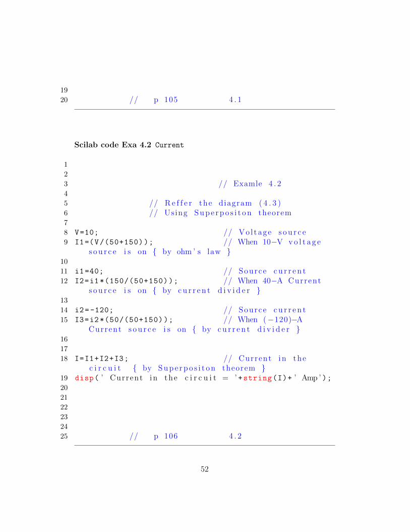
Scilab code Exa 4.2 Current
1
2
3 // Examle 4 . 24
5 // R e f f e r the diagram ( 4 . 3 )6 // Using S u p e r p o s i t o n theorem7
8 V=10; // Vo l tage s o u r c e9 I1=(V/(50+150)); // When 10−V v o l t a g e
s o u r c e i s on { by ohm ’ s law }10
11 i1=40; // Source c u r r e n t12 I2=i1 *(150/(50+150)); // When 40−A Current
s o u r c e i s on { by c u r r e n t d i v i d e r }13
14 i2= -120; // Source c u r r e n t15 I3=i2 *(50/(50+150)); // When (−120)−A
Current s o u r c e i s on { by c u r r e n t d i v i d e r }16
17
18 I=I1+I2+I3; // Current i n thec i r c u i t { by S u p e r p o s i t o n theorem }
19 disp( ’ Current i n the c i r c u i t = ’ +string(I)+ ’ Amp ’ );20
21
22
23
24
25 // p 106 4 . 2
52
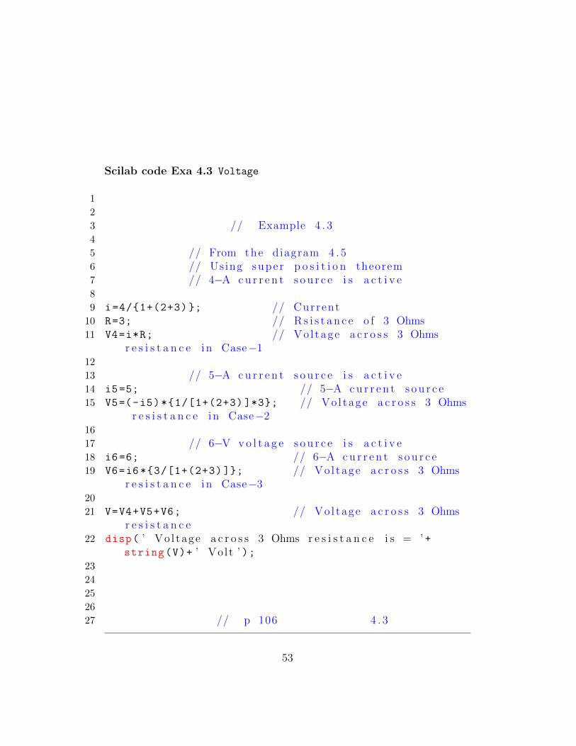
Scilab code Exa 4.3 Voltage
1
2
3 // Example 4 . 34
5 // From the diagram 4 . 56 // Using supe r p o s i t i o n theorem7 // 4−A c u r r e n t s o u r c e i s a c t i v e8
9 i=4/{1+(2+3) }; // Current10 R=3; // R s i s t a n c e o f 3 Ohms11 V4=i*R; // Vo l tage a c r o s s 3 Ohms
r e s i s t a n c e i n Case−112
13 // 5−A c u r r e n t s o u r c e i s a c t i v e14 i5=5; // 5−A c u r r e n t s o u r c e15 V5=(-i5)*{1/[1+(2+3) ]*3}; // Vo l tage a c r o s s 3 Ohms
r e s i s t a n c e i n Case−216
17 // 6−V v o l t a g e s o u r c e i s a c t i v e18 i6=6; // 6−A c u r r e n t s o u r c e19 V6=i6 *{3/[1+(2+3) ]}; // Vo l tage a c r o s s 3 Ohms
r e s i s t a n c e i n Case−320
21 V=V4+V5+V6; // Vo l tage a c r o s s 3 Ohmsr e s i s t a n c e
22 disp( ’ Vo l tage a c r o s s 3 Ohms r e s i s t a n c e i s = ’ +string(V)+ ’ Vo l t ’ );
23
24
25
26
27 // p 106 4 . 3
53

Scilab code Exa 4.4 Current
1
2
3 // Examle 4 . 44
5 // From the diagram ( 4 . 6 a )6 // Using S u p e r p o s i t o n theorem7
8 V=10; // Vo l tage s o u r c e9 I1=(V/(2+4+6)); // When 10−V v o l t a g e
s o u r c e i s on { by ohm ’ s law }10
11 // we have to f i n d I s=?
12 // When Is−A Currents o u r c e i s on
13 // w i l l have { I 2=−(2/3) I s }
14 // g i v e n tha t I1+I2= 015 // t h e r e f o r 5/6 −
( 2 / 3 ) I s= 016 Is =(5*3) /(6*2); // Source c u r r e n t17 disp( ’ The v a l u e o f s o u r c e c u r r e n t ( I s ) = ’ +string(
Is)+ ’ Amp ’ );18
19
20
21
22
23 // p 108 4 . 4
54
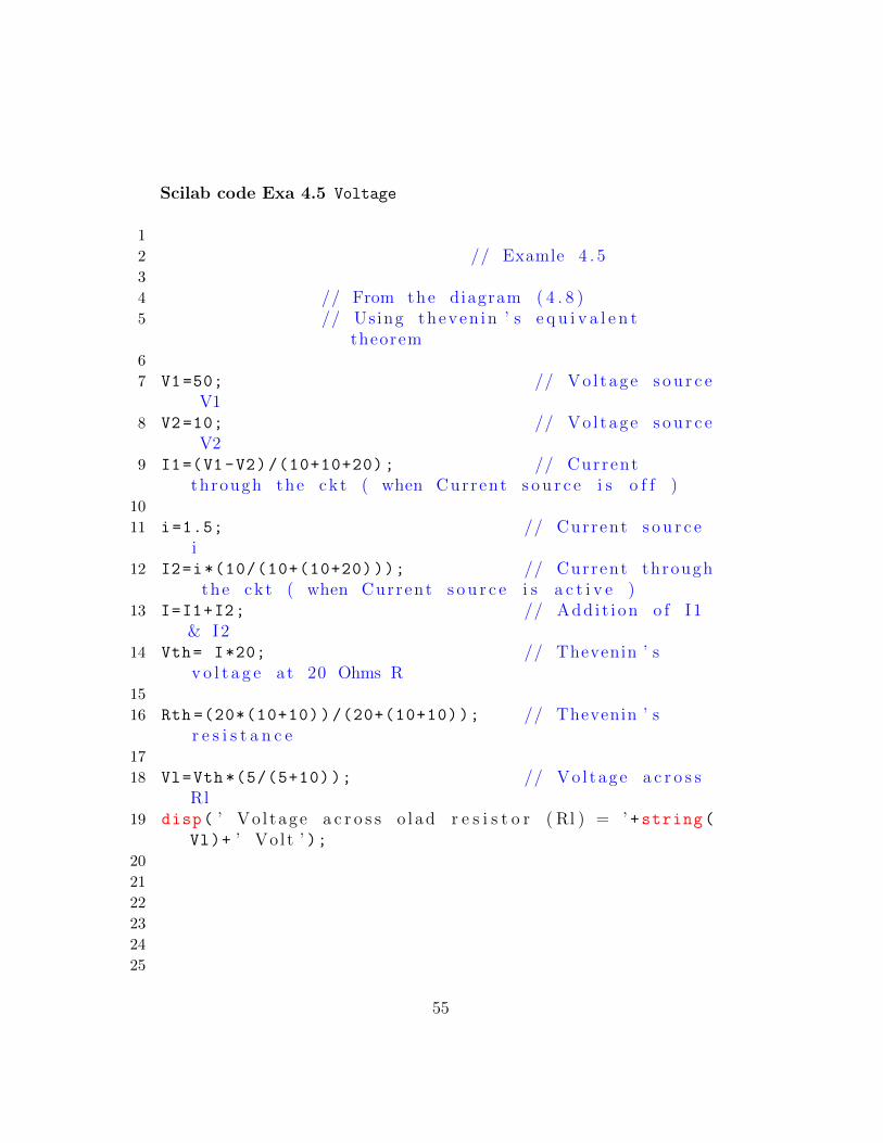
Scilab code Exa 4.5 Voltage
1
2 // Examle 4 . 53
4 // From the diagram ( 4 . 8 )5 // Using theven in ’ s e q u i v a l e n t
theorem6
7 V1=50; // Vo l tage s o u r c eV1
8 V2=10; // Vo l tage s o u r c eV2
9 I1=(V1-V2)/(10+10+20); // Currentthrough the ck t ( when Current s o u r c e i s o f f )
10
11 i=1.5; // Current s o u r c ei
12 I2=i*(10/(10+(10+20))); // Current throughthe ck t ( when Current s o u r c e i s a c t i v e )
13 I=I1+I2; // Add i t i on o f I 1& I2
14 Vth= I*20; // Thevenin ’ sv o l t a g e at 20 Ohms R
15
16 Rth =(20*(10+10))/(20+(10+10)); // Thevenin ’ sr e s i s t a n c e
17
18 Vl=Vth *(5/(5+10)); // Vo l tage a c r o s sRl
19 disp( ’ Vo l tage a c r o s s o l ad r e s i s t o r ( Rl ) = ’ +string(Vl)+ ’ Vo l t ’ );
20
21
22
23
24
25
55
26 // p 110 4 . 5
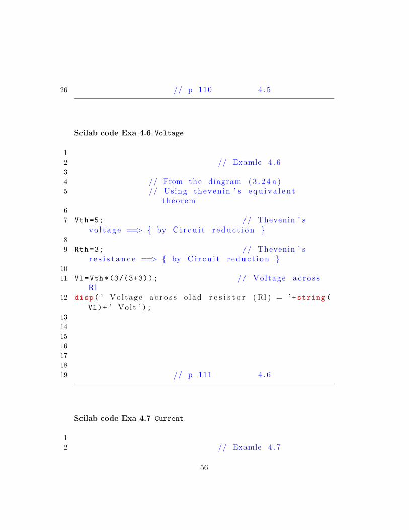
Scilab code Exa 4.6 Voltage
1
2 // Examle 4 . 63
4 // From the diagram ( 3 . 2 4 a )5 // Using theven in ’ s e q u i v a l e n t
theorem6
7 Vth =5; // Thevenin ’ sv o l t a g e ==> { by C i r c u i t r e d u c t i o n }
8
9 Rth =3; // Thevenin ’ sr e s i s t a n c e ==> { by C i r c u i t r e d u c t i o n }
10
11 Vl=Vth *(3/(3+3)); // Vo l tage a c r o s sRl
12 disp( ’ Vo l tage a c r o s s o l ad r e s i s t o r ( Rl ) = ’ +string(Vl)+ ’ Vo l t ’ );
13
14
15
16
17
18
19 // p 111 4 . 6
Scilab code Exa 4.7 Current
1
2 // Examle 4 . 7
56

3
4 // From the diagram ( 4 . 1 1 a )5
6 // Using Nortan ’ se q u i v a l e n t theorem
7
8 R1=5; // R e s i s t a n c e R19 R2=10; // R e s i s t a n c e R2
10 V1=10; // Vo l tage s o u r c e V111 I1=V1/R1; // Current I112
13 V2=5; // Vo l tage s o u r c e V214 I2=V2/R2; // Current I215 IN=I1+I2; // Nortan ’ s c u r r e n t16
17 RN=(R1*R2)/(R1+R2); // Nortan ’ s r e s i s t a n c e18
19 Rl=5; // Load r e s i s t a n c e20 Il=IN*(RN/(RN+Rl)); // Load c u r r e n t21 disp( ’ Load c u r r e n t ( I l ) = ’ +string(Il)+ ’ Amp ’ );22
23
24
25 // p 113 4 . 7
Scilab code Exa 4.8 Power
1
2 // Examle 4 . 83
4 Voc =12.6; // Vo l tage o f c a r b a t t e r y5 Isc =300; // Short−c i r c u i t c u r r e n t6 Ro=Voc/Isc; // O/p r e s i s t a n c e7
8 // { P=Vht ˆ2/4 Rth } , but
57
he r e Vth= Voc & Rth= Ro9 Pavl=Voc ^2/(4* Ro); // A v a i l a b l e power10 disp( ’ A v a i l a b l e power i s = ’ +string(Pavl)+ ’ Watt ’ )
;
11
12
13
14
15
16 // p 114 4 . 8
Scilab code Exa 4.9 Power
1
2 // Examle 4 . 93
4 n=8; // No . Of dry c e l l s5 E=1.5; // Emf o f c e l l6 Voc=n*E; // open−c i r c u i t Vo l tage
o f b a t t e r y7 r=0.75; // I n t e r n a l r e s i s t a n c e8 Ro=r*n; // O/p r e s i s t a n c e9
10 // ==> { P=Vht ˆ2/4 Rth } , but he r e Vth= Voc & Rth= Ro
11
12 Pavl=Voc ^2/(4* Ro); // A v a i l a b l e power13 disp( ’ A v a i l a b l e power i s = ’ +string(Pavl)+ ’ Watt ’ )
;
14
15
16
17
18
19 // p 115 4 . 9
58
Scilab code Exa 4.10 Voltage And Power
1
2 // Examle 4 . 1 03
4 // From Diagram 4 . 1 25
6 P=25; // Power7 Rl=8; // Load
r e s i s t a n c e8 Vth=P*4*Rl; // Thevenin ’ s
e q u i v a l e n t v o l t a g e9
10 // I f Load i s Short−ck t (RL=0)11 Vo=0; // Vo l tage12 IL=1; // l oad c u r r e n t13 Po1=Vo*IL; // O/p power14
15 // I f Load i s Open−ck t ( RL=i n f i n i t y )16 IL1 =0; // Load c u r r e n t17 Vo1 =1; // Vo l tage18 Po2=Vo1*IL1; // O/p power19
20 x=[0 2 4 6 8 16 32 ]; // D i f f r e n t v a l u eo f RL
21 y=[0 16 22.22 24.49 25 22.22 16 ] // Value o f Power22
23 plot2d(x,y); // To p l o t graph24 xlabel( ’RL ( i n Ohms )−−−> ’ ); // For X−Labe l25 ylabel( ’ Po ( i n W −−−−> ’ ) // For Y−Labe l26
27
28
29 // View p 115 4 . 1 0
59
Scilab code Exa 4.11 Current And Resistance
1
2 // Examle 4 . 1 13
4 // From the diagram ( 4 . 1 4 )5
6 Req =2+{(12*4) /(12+4) }+4; // E q u i v a l e n tr e s i s t a n c e ( f o r 4 . 1 4 a )
7 v=36; // Vo l tages o u r c e
8 i=v/Req; // Currentsupp ly by the v o l t a g e s o u r c e
9 I=i*(12/(12+4)); // Current i nbranch B ==> { by c u r r e n t d i v i d e r }
10 disp( ’ Current i n branch B = ’ +string(I)+ ’ Amp ’ );11
12 Req1 =3+{(12*6) /(12+6) }+1; // E q u i v a l e n tr e s i s t a n c e ( f o r 4 . 1 4 b )
13 i1=v/Req1; // Currentsupp ly by the v o l t a g e s o u r c e
14 I1=i1 *(12/(12+6)); // Current i nbranch A ==> { by c u r r e n t d i v i d e r }
15 disp( ’ Current i n branch A = ’ +string(I1)+ ’ Amp ’ );16
17 Rtr=v/I; // T r a n s f e rr e s i s t a n c e
18 disp( ’ T r a n s f e r r e s i s t a n c e from Branch A to B = ’ +string(Rtr)+ ’ Ohm ’ );
19
20
21
22 // p 117 4 . 1 1
60
Chapter 5
Electromagnetism
Scilab code Exa 5.1 Current
1
2
3 // Example 5 . 14
5 B=20*10^ -3; // Megnet ic F i e l d i n t e n s i t y6 m=4*%pi *10^ -7; // P e r m e a b i l i t y o f f r e e Space7 n=20*100; // No . Of Turns per meter8 I=B/(m*n);
9 disp( ’ Ne c e s s a ry Current i s = ’ +string(round(I))+ ’Amp ’ );
10
11
12
13 // p 187 5 . 1
Scilab code Exa 5.2 Megnetic Field Strength
1
61
2
3
4 // Example 5 . 25
6 l=4; // Layer s o f S o l e n o i d7 w=350; // t u r n s Winding8 s=0.5; // Length o f S o l e n o i d9 n=(l*w)/s; // No . Of t u r n s
10 I=6; // Current i n the S o l e n o i d11 mo=4*%pi *10^ -7; // P e r m e a b i l i t y o f f r e e Space12 B=mo*n*I; // Formula f o r Megnet ic F i e l d at
the c e n t r e13 disp( ’ ( a ) Megnitude o f f i e l d near the Centre o f
S o l e n o i d = ’ +string(B)+ ’ Te s l a ’ );14 B1=B/2; // Formula f o r Megnet ic F i e l d at
the end15 disp( ’ ( b ) Megnitude o f f i e l d at the end o f S o l e n o i d
= ’ +string(B1)+ ’ Te s l a ’ );16 disp( ’ ( c ) Megnet ic F i e l d o u t s i d e the s o l e n o i d i s
N e g l i g i b l e ’ );17
18
19
20 // p 188 5 . 2
Scilab code Exa 5.3 Force
1
2
3 // Example 5 . 34
5 mo=4*%pi *10^ -7; // P e r m e a b i l i t y o f f r e e Space6 i1=80; // Current i n 1 s t Wire7 i2=30; // Current i n 2nd Wire8 r=2; // D i s t a n c e between 2 w i r e s
62
9
10 F=(mo*i1*i2)/(2* %pi*r);
11 disp( ’ Force between 2 w i r e s = ’ +string(F)+ ’ N/m’ );12
13
14
15
16
17 // p 192 5 . 3
Scilab code Exa 5.4 Force
1
2
3
4 // Example 5 . 45
6 mo=4*%pi *10^ -7; // P e r m e a b i l i t y o f f r e e Space7 i1=4; // Current i n 1 s t Wire8 i2=6; // Current i n 2nd Wire9 r=0.03; // D i s t a n c e between 2 w i r e s
10
11 F=(mo*i1*i2)/(2* %pi*r);
12 l=0.15; // S e c t i o n o f w i r e13 Fnet=F*l;
14 disp( ’ Force on 15 cm o f w i r e B i s = ’ +string(Fnet)+’ N ’ );
15
16
17
18
19
20 // p 192 5 . 4
63
Scilab code Exa 5.5 Voltage
1
2
3
4 // Example 5 . 55
6 B=0.5; // Megnet ic F i e l d7 l=0.2; // Length o f conduc to r8 v=5; // v e l o c i t y Conductor9 Q1=0; // Angle o f Motion i n c a s e 1
10 Q2=90; // Angle o f Motion i n c a s e 211 Q3=30; // Angle o f Motion i n c a s e 312
13 e1=B*l*v*sind(Q1);
14 disp( ’ emf o f conduc to r when move P a r a l l e l toMegnet ic f i e l d = ’ +string(e1)+ ’ Vo l t ’ );
15 e2=B*l*v*sind(Q2);
16 disp( ’ emf o f conduc to r when move P e r p e n d i c u l a r toMegnet ic f i e l d = ’ +string(e2)+ ’ Vo l t ’ );
17 e3=B*l*v*sind(Q3);
18 disp( ’ emf o f conduc to r when move at an Angle 30 toMegnet ic f i e l d = ’ +string(e3)+ ’ Vo l t ’ );
19
20
21
22
23
24 // p 198 5 . 5
Scilab code Exa 5.6 Voltage
64
1
2
3
4
5 // Example 5 . 66
7 B=38*10^ -6; // Megnet ic F i e l d8 l=52; // Length o f conduc to r9 Q=90; // Angle o f Motion i n c a s e 1
10 v=(1100*1000) /3600; // v e l o c i t y i n m/ s11 e=B*l*v*sind(Q); // Formula o f emf12 disp( ’ emf Generated between wing−t i p s = ’ +string(e)
+ ’ Vo l t ’ );13
14
15
16
17
18 // p 198 5 . 6
Scilab code Exa 5.7 Voltage
1
2
3
4
5
6 // Example 5 . 77
8 // We know tha t Area o f Ring i s (A=Pi ∗R∗R)
9 // i . e A=%pi∗R∗R∗ (Q/2 %pi ) =0.5∗R∗R∗Q;
10 // Hance by u s i n g Faraday ’ s Law11 // e= dQ/ dt= d (BA) / dt .
65

12 // 0 . 5∗B∗R∗R∗ ( dq/ dt ) .13
14 B=1;
15 R=1;
16 f=50;
17 e=0.5*B*R*R*f*2*%pi; // by u s i n g Faraday ’ s Law18
19 disp( ’ emf Devloped between Centre & r i n g = ’ +string(round(e))+ ’ Vo l t ’ );
20
21
22 // p 198 5 . 7
Scilab code Exa 5.8 Voltage Time And Force
1
2
3 // Example 5 . 84
5
6 B=0.5; // Megnet ic F i e l d7 l1 =0.03; // Length o f conduc to r8 v=0.01; // v e l o c i t y i n m/ s9 e1=B*l1*v; // Formula o f emf10 disp( ’ ( a ) The induced emf i s = ’ +string(e1)+ ’ Vo l t ’ )
;
11 l2=0.1; // Length12 t1=l2/v;
13 disp( ’ Time f o r which the induced Vo l tage l a s t s i s =’ +string(t1)+ ’ Second ’ );
14
15 e2=B*l2*v; // Formula o f emf16 disp( ’ ( b ) The induced emf i s = ’ +string(e2)+ ’ Vo l t ’
);
17 t2=l1/v;
66
18 disp( ’ Time f o r which the induced Vo l tage l a s t s i s =’ +string(t2)+ ’ Second ’ );
19 disp( ’ ( c ) Because o f the gap , No Current can f l o w .t h e r e f o r no f o r c e Requ i red to P u l l the c o i l . ’ );
20 R=0.001;
21 F1=(B*B*l1*l1*v)/R; // Formula o f Force22 disp( ’ ( d . 1 ) Force Requ i red to p u l l the l oop 1 = ’ +
string(F1)+ ’ N ’ );23 F2=(B*B*l2*l2*v)/R; // Formula o f Force24 disp( ’ ( d . 2 ) Force Requ i red to p u l l the l oop 1 = ’ +
string(F2)+ ’ N ’ );25
26
27 // p 199 5 . 8
67
Chapter 6
Magnetic Circuits
Scilab code Exa 6.1 Megnetic Field Strength And Flux
1
2 // Example 6 . 13
4 N=200; // No . Of t u r n s5 I=4; // Current o f a C o i l6 l=.06; // c i r c u m f e r e n c e o f C o i l7 H=(N*I)/l; // Formula o f Megnet ic F i e l d
S t r e n g t h8 disp( ’ ( a ) The Megnet ic F i e l d S t r e n g t h = ’ +string(H)+
’ A/m’ );9 mo=4*%pi *10^ -7; // P e r m e a b i l i t y o f f r e e Space
10 mr=1; // P e r m e a b i l i t y o f c o i l11 B=mr*mo*H; // Formula o f Flux Dens i ty12 disp( ’ ( b ) The Flux Dens i ty i s = ’ +string(B)+ ’ Te s l a ’
);
13 A=500*10^ -6; // Area o f C o i l14 Q=B*A; // Tota l Flux15 disp( ’ ( c ) The t o t a l Flux i s = ’ +string(Q)+ ’ Wb’ );16
17
18
68
19 // p 211 6 . 1
Scilab code Exa 6.2 Megnetomotive Force
1
2
3 // Example 6 . 24
5 Q=0.015; // Flux6 A=200*10^ -4; // Area o f Conductor7 mo=4*%pi *10^ -7; // P e r m e a b i l i t y o f f r e e Space8 B=Q/A; // Megnet ic Flux Dens i ty9 H=B/mo; // Megnet ic F i e l d S t r e n g t h
10 l=2.5*10^ -3; // Air Gap11 F=H*l; // Formula o f Magnetomotive Force
(mmf)12
13 disp( ’ Magnetomotive Force (mmf) i s = ’ +string(round(F))+ ’ At ’ );
14
15
16
17
18 // p 212 6 . 2
Scilab code Exa 6.3 Reluctance And Current
1
2
3
4 // Example 6 . 35
6 Q=800*10^ -6; // Flux
69
7 A=500*10^ -6; // Area o f C o i l8 mo=4*%pi *10^ -7; // P e r m e a b i l i t y o f f r e e Space9 mr=380; // P e r m e a b i l i t y o f o f C o i l10 l=0.4; // c i r c u m f e r e n c e o f C o i l11 R=l/(mr*mo*A); // Formula o f Re lu c tance12 disp( ’ Re lu c tance o f Ring i s = ’ +string(R)+ ’ A/Wb’ );13 F=Q*R; // Formula o f Magnetomotive Force
(mmf)14 N=200; // No . Of t u r n s15 I=F/N; // Formula o f Magne t i s i ng Current16 disp( ’ Magne t i s i ng Current i s = ’ +string(I)+ ’ At ’ );17
18
19
20 // p 212 6 . 3
Scilab code Exa 6.4 Current
1
2
3 // Example 6 . 44
5 B=0.9; // Megnet ic Flux Dens i ty6 N=4000; // No . Of t u r n s7 mo=4*%pi *10^ -7; // P e r m e a b i l i t y o f f r e e Space8 Hc=820; // Megnet ic F i e l d S t r e n g t h f o r
Core9 lc =0.22; // Length o f C i r c u i t
10 Ac=50*10^ -6; // Area o f C i r c u i t11 Fc=Hc*lc; // Magnetomotive Force (mmf) f o r
Core12 lg =0.001; // Length o f Air Gap13 Ag=50*10^ -6; // Area o f Megnet ic C i r c u i t14 Hg=B/mo; // Megnet ic F i e l d S t r e n g t h f o r
Air Gap
70

15 Fg=Hg*lg; // Magnetomotive Force (mmf) f o rAir Gap
16 F=Fc+Fg; // Tota l Magnetomotive Force (mmf)
17 I=F/N; // Formula o f Magne t i s i ng Current18 disp( ’ Magne t i s i ng Current i s = ’ +string(I)+ ’ Amp ’ );19
20
21
22
23 // p 215 6 . 4
71
Chapter 7
Self And Mutual Inductances
Scilab code Exa 7.1 Voltage
1
2
3 // Example 7 . 14
5 L=4; // I n d u c t i o n o f a C o i l6 di=10-4; // Dec r ea s e i n Current7 dt=0.1; // t ime Requ i red to Dec r ea s e
Current8 e=L*(di/dt); // Formula o f S e l f i n d u c t i o n9 disp( ’ emf induced i n a C o i l i s = ’ +string(e)+ ’ Vo l t
’ );10
11
12
13 // p 228 7 . 1
Scilab code Exa 7.2 Inductor And Voltage
72
1
2
3
4 // Example 7 . 25
6 N=150; // t u r n s o f C o i l7 Q=0.01; // Flux o f C o i l8 I=10; // Current i n C o i l9 L=N*(Q/I); // I n d u c t i o n o f a C o i l
10 di=10-( -10); // Dec r ea s e i n Current11 dt =0.01; // t ime Requ i red to Dec r ea s e
Current12 e=L*(di/dt); // Formula o f S e l f i n d u c t i o n13 disp( ’ I n d u c t i o n o f a C o i l = ’ +string(L)+ ’ H ’ );14 disp( ’ emf induced i n a C o i l i s = ’ +string(e)+ ’ Vo l t
’ );15
16
17
18 // p 228 7 . 2
Scilab code Exa 7.3 Inductor And Voltage
1
2
3
4
5 // Example 7 . 36
7 N=100; // t u r n s o f C o i l8 dQ=0.4 -( -0.4); // Flux o f C o i l9 di=10-( -10); // Dec r ea s e i n Current
10 L=N*(dQ/di)*10^ -3; // I n d u c t i o n o f a C o i l11 disp( ’ ( a ) i n d u c t i o n o f a C o i l i s = ’ +string(L)+ ’ H ’
);
73
12 dt =0.01; // t ime Requ i red to Dec r ea s eCurrent
13 e=L*(di/dt); // Formula o f emf ( u s i n g S e l fi n d u c t i o n )
14 disp( ’ ( b ) emf induced i n a C o i l i s = ’ +string(e)+ ’Vo l t ’ );
15
16
17
18 // p 229 7 . 3
Scilab code Exa 7.4 Inductor And Energy
1
2
3 // Example 7 . 44
5 r=0.75*10^ -2; // Radius o f S o l e n o i d6 A=%pi*r*r; // a r ea o f S o l e n o i d7 N=900; // No , o f t u r n s8 l=0.3; // Length o f S o l e n o i d9 mo=4*%pi *10^ -7; // P e r m e a b i l i t y o f f r e e Space
10 L=(N*N*mo*A)/l; // Formula o f I n d u c t i o n o f a C o i l11 I=5; // Current o f C o i l12 disp( ’ I n d u c t i o n o f a C o i l = ’ +string(L)+ ’ H ’ );13 w=0.5*L*I*I; // Energy S t o r e14 disp( ’ Energy Sto r ed i s = ’ +string(w)+ ’ J ’ );15
16
17
18 // p 229 7 . 4
Scilab code Exa 7.5 Megnetic Field Strength And Voltage
74

1
2 // Example 7 . 53
4 r=1*10^ -2; // Radius o f rod5 A=%pi*r*r; // a r ea o f rod6 N=3000; // No . o f t u r n s7 I=0.5; // Current i n the rod8 l=0.2; // Diameter o f rod9 B=1.2; // Megnet ic Flux Dens i ty10 H=(N*I)/l; // Megnet ic F i e l d S t r e n g t h11 m=B/H; // P e r m e a b i l i t y o f rod12 disp( ’ ( a ) P e r m e a b i l i t y o f i r o n = ’ +string(m)+ ’ Tm/A
’ );13 mo=4*%pi *10^ -7; // P e r m e a b i l i t y o f f r e e Space14 mr=m/mo; // r e l a t i v e P e r m e a b i l i t y15 disp( ’ ( b ) R e l a t i v e P e r m e a b i l i t y o f i r o n = ’ +string(
round(mr)));
16 Q=B*A; // Flux17 dQ=Q*0.9; // Chenge i n Flux18 L=(N*Q)/I; // Formula o f I n d u c t i o n o f a
C o i l19 disp( ’ ( c ) I n d u c t i o n o f a C o i l = ’ +string(L)+ ’ H ’ );20 di =0.01;
21 e=N*(dQ/di) // Formula o f emf ( u s i n g S e l fi n d u c t i o n )
22 disp( ’ ( d ) Vo l tage i n a C o i l = ’ +string(e)+ ’ Vo l t ’ );23
24
25
26 // p 229 7 . 5
Scilab code Exa 7.6 Voltage
1
2
75
3 // Example 7 . 64
5 i=1; // Current i n A C o i l6 R=3; // R o f C o i l7 L=0.1*10^ -3; // Induc tance o f C o i l8 di =10000; // Dec r ea s e i n Current9 dt=1; // t ime Requ i red to Dec r ea s e
Current10 V=(i*R)+L*(di/dt); // Formula Of P o t e n t i a l
D i f f r e n c e11 disp( ’ P o t e n t i a l D i f f r e n c e Acros s the Terminal i s =
’ +string(V)+ ’ Vo l t ’ );12
13
14
15
16 // p 230 7 . 6
Scilab code Exa 7.7 Inductor And Voltage
1
2 // Example 7 . 73
4 k=1; // Constant5 N1 =2000; // t u r n s o f S o l e n o i d6 N2=500; // t u r n s o f C o i l7 mo=4*%pi *10^ -7; // P e r m e a b i l i t y o f f r e e Space8 A=30*10^ -4; // Area o f a C o i l9 l=0.7; // Length o f S o l e n o i d
10 z=k*N1*N2*mo*A; // a l p h a b e t f o r s i m p l i c i t y11 M=z/l; // Formula o f Mutual
Induc tance12 disp( ’ ( a ) Mutual i n d u c t i o n o f a C o i l = ’ +string(M)+ ’
H ’ );13 dit =260; // Rate o f Chenge o f Current
76

14 e=M*dit; // Formula o f emf ( u s i n gMutual i n d u c t i o n )
15 disp( ’ ( b ) emf induced i n a C o i l i s = ’ +string(e)+ ’Vo l t ’ )
16
17
18
19
20 // p232 7 . 7
Scilab code Exa 7.8 Inductor
1
2 // Example 7 . 83
4 N2 =1700; // t u r n s o f C o i l 15 Q2 =0.8*10^ -3; // t o t a l Megnet ic Flux6 I2=6; // Current i n A C o i l 27 L2=N2*(Q2/I2); // Formula f o r ( S e l f
I nduc tance o f C o i l 1 )8 disp( ’ ( a ) S e l f I n d u c t i o n o f a C o i l 2 = ’ +string(L2)+
’ H ’ );9 N1=600; // t u r n s o f C o i l 210 L1=L2*(N1^2/N2^2); // Formula f o r ( S e l f
I nduc tance o f C o i l 2 )11 disp( ’ ( b ) S e l f I n d u c t i o n o f a C o i l 1 = ’ +string(L1)+
’ H ’ );12 Q21 =0.5*10^ -3; // Megnet ic Flux i n 1 s t
C o i l13 k=Q21/Q2; // Constant14 disp( ’ ( c ) P e r p o s n a l i t y Constant ( k ) = ’ +string(k));15 M=k*sqrt(L1*L2); // Mutual Induc tance o f
C o i l 1 & 216 disp( ’ ( d ) Mutual i n d u c t i o n o f a C o i l = ’ +string(M)+ ’
H ’ );
77
17
18
19
20 // p 233 7 . 8
Scilab code Exa 7.9 Inductor
1
2
3 // Example 7 . 94
5 N2=800; // t u r n s o f C o i l 26 N1 =1200; // t u r n s o f C o i l 17 Q2 =0.15*10^ -3; // Megnet ic Flux i n C o i l 28 Q1 =0.25*10^ -3; // Megnet ic Flux i n C o i l 19 I2=5; // Current i n A C o i l 210 I1=5; // Current i n A C o i l 111
12 L1=N1*(Q1/I1); // Formula f o r ( S e l fI nduc tance o f C o i l 1 )
13 disp( ’ ( a ) S e l f I n d u c t i o n o f a C o i l 1 = ’ +string(L1)+’ H ’ );
14
15 L2=N2*(Q2/I2); // Formula f o r ( S e l fI nduc tance o f C o i l 2 )
16 disp( ’ ( b ) S e l f I n d u c t i o n o f a C o i l 2 = ’ +string(L2)+’ H ’ );
17
18 k=0.6; // C o e f f i c i e n t o f Coupl ingConstant
19 Q12=k*Q1; // Formula f o r ( Megnet icFlux i n 2nd C o i l )
20 M=N2*(Q2/I1); // Formula f o r ( MutualInduc tance o f C o i l s )
21 disp( ’ ( c ) Mutual i n d u c t i o n o f a C o i l = ’ +string(M)+ ’
78
H ’ );22
23 k1=M/sqrt(L1*L2); // Mutual Induc tance o fC o i l 1 & 2
24 disp( ’ ( d ) C o e f f i c i e n t o f Coupl ing between the C o i l =’ +string(k1)+ ’ H ’ );
25
26
27
28 // p 233 7 . 9
Scilab code Exa 7.10 Inductor
1
2
3 // Example 7 . 1 04
5 La=1.4; // Induc tance o f 2 S i m i l a rCoupled C o i l i n S e r i e s
6 Lo=0.6; // Induc tance o f 2 S i m i l a rCoupled C o i l i n Opposing
7 M=(La -Lo)/4; // Formula f o r ( MutualInduc tance o f C o i l s )
8 disp( ’ ( a ) Mutual i n d u c t i o n o f a C o i l = ’ +string(M)+ ’mH’ );
9
10 // S i n c e La= L1+L2+2M but (M=0.2mH)
11 // t h e r e f o r L1= L2= 5 mh12
13 L1 =0.5*10^ -3; // S e l f Induc tance o fC o i l 1
14 L2 =0.5*10^ -3; // S e l f Induc tance o fC o i l 2
15 k=(M*10^ -3)/sqrt(L1*L2); // Mutual Induc tance o f
79

C o i l 1 & 216 disp( ’ ( b ) C o e f f i c i e n t o f Coupl ing between the C o i l s
= ’ +string(k));17
18
19
20
21 // p136 7 . 1 0
Scilab code Exa 7.11 Inductor
1
2
3 // Example 7 . 1 14
5 // Net I n d u c t i o n When i n SameD i r e c t i o n i . e 1.8= L1+L2+2M
6 // Net I n d u c t i o n When i n Oppos i t e i . e0.8= L1+L2−2M
7 // by S o l v i n g 2 e q u a t i o n we ge t M=0 . 2 5
8 k=0.6;
9 M=0.25;
10 disp( ’ ( a ) Mutual i n d u c t i o n o f a C o i l = ’ +string(M)+ ’H ’ );
11 // by Adding Eq 1 & 2 w i l l g e t L1+L2= 1 . 3 H
12 // we know tha t k= M/( L1∗L2 )13 L1L2=M^2/k^2; // u s i n g above Formula14 // By u s i n g L1L2 & L1+L215 L12 =1.3; // L1+L216 L1_L2=sqrt(L12^2-4* L1L2); // Value o f L1−L217
18 // by u s i n g L1+L2 & L1−L2 w i l l g e t19
80
20 L1 =1.149;
21 L2 =0.151;
22 disp( ’ ( b . 1 ) S e l f I n d u c t i o n o f a C o i l 1 = ’ +string(L1)+ ’ H ’ );
23 disp( ’ ( b . 2 ) S e l f I n d u c t i o n o f a C o i l 2 = ’ +string(L2)+ ’ H ’ );
24
25
26
27 // p 237 7 . 1 1
Scilab code Exa 7.12 Inductor
1
2
3 // Example 7 . 1 24
5 k=0.433; // C o e f f i c i e n t o fCoupl ing Constant
6 L1=8; // S e l f I nduc tance o fC o i l 1
7 L2=6; // S e l f I nduc tance o fC o i l 2
8 M=k*sqrt(L1*L2); // Mutual Induc tance o fC o i l 1 & 2
9
10 Lpa=(L1*L2-M^2)/(L1+L2 -2*M); // Mutual I n d u c t i o na s s i s t s S e l f I n d u c t i o n
11 disp( ’ ( a ) Mutual I n d u c t i o n a s s i s t s S e l f I n d u c t i o n =’ +string(Lpa)+ ’ H ’ );
12
13 Lpo=(L1*L2-M^2)/(L1+L2+2*M); // Mutual I n d u c t i o nOpposes S e l f I n d u c t i o n
14 disp( ’ ( b ) Mutual I n d u c t i o n Opposes S e l f I n d u c t i o n =’ +string(Lpo)+ ’ H ’ );
81
15
16
17
18
19
20 // p 239 7 . 1 2
82
Chapter 8
DC Transients
Scilab code Exa 8.1 Voltage
1
2 // Example 8 . 13
4 // From diagram 8 . 35
6 // E q u i v a l e n t r e s i s t a n c e i . e Req= 20+( 2 0 | | 1 0 )
7
8 Req= 20+{(20*10) /(20+10) }; // E q u i v a l e n tr e s i s t a n c e
9 V=24; // Supply v o l t a g e10 I=V/Req; // Supply c u r r e n t11 R=20; // R e s i s t a n c e12 R1 =20+10; // Tota l
R e s i s t a n c e [ from Fig 8 . 3 b ]13 Il=I*{20/(20+10) }; // Current through
i n d u c t o r14 io=Il; // Open−ck t
c u r r e n t15 disp( ’ Open−ck t c u r r e n t = ’ +string(io)+ ’ Amp ’ );16
83

17 Vr=-io*R; // Vo l tage a c r o s s20 Ohms r e s i s t o r
18 disp( ’ Vo l tage a c r o s s 20 Ohms r e s i s t o r = ’ +string(Vr)+ ’ Vo l t ’ );
19
20 // Vo l tage a c r o s s i n d u c t o r i s g i v e n by i . e[ e=L∗{ i o ∗ (R/L) } ]
21 // tha t i s [ e= i o ∗R ]22
23 e=io*R1; // Vo l tage a c r o s si n d u c t o r
24 disp( ’ Vo l tage a c r o s s i n d u c t o r = ’ +string(e)+ ’ Vo l t ’);
25
26
27
28
29 // p 276 8 . 1
Scilab code Exa 8.2 Current And Power
1
2 // Example 8 . 23
4
5 R=0.8; // R e s i s t a n c e6 L=1.6; // I n d u c t o r7 t1=L/R; // Time8
9 // I n s t a n t a n e o u s c u r r e n t i s ( i t= Io ∗ e(−t /2) )
10
11 Io=20/ exp (0.5); // The c u r r e n t ( at t= −1 & i=20A )
12 disp( ’ The v a l u e o f c u r r e n t at t=0 i ( 0 ) = ’ +string(
84
Io)+ ’ Amp ’ );13
14 i1=Io*exp ( -0.5); // Current through i n d u c t o r att= 1S
15 i=7.36; // i 1 =7.357 we have taken as (i =7.36 )
16 p1=i*i*R; // Power absorbed by R e s i s t o r17 disp( ’ Power absorbed by i n d u c t o r at t= 1S P( 1 ) = ’ +
string(-p1)+ ’ Watt ’ );18
19 // We know tha t w=0.5∗L∗ i t ˆ 2 ; w= 100 J20
21 it=sqrt (200/1.6); // Flow o f c u r r e n t22 t=log (Io/it)*2; // Time r e q u i r e d to s t o r e
Energy 100 J23 disp( ’ Time r e q u i r e d to s t o r e Energy 100 J = ’ +string
(t)+ ’ Second ’ );24
25
26
27 // p 277 8 . 2
Scilab code Exa 8.3 Current And Time
1
2
3 // Example 8 . 34
5 R=10; // R e s i s t a n c e6 L=14; // I n d u c t o r7 t1=L/R; // Time8
9 V=140; // Vo l tage10 Io=V/R; // Steady S t a t e c u r r e n t11 t2=0.4; // Time
85
12 i=Io*(1-exp (-t2/t1)); // Value o f c u r r e n t at t= 0 . 4
13 disp( ’ Value o f c u r r e n t at ( t =0.4) = ’ +string(i)+ ’Amp ’ );
14
15 // ==> We have fo rmu la i t=Io ∗ exp (− t /t1 ) .
16 it=8; // Current o f 8 Amp17 t=-log(it/14)*t1; // Time taken to r e ch at
i =8 A18 disp( ’ Time taken to r e ch at i =8 A = ’ +string(t)+ ’
Second ’ );19
20
21
22
23 // p 279 8 . 3
Scilab code Exa 8.4 Current
1
2 // Example 8 . 43
4 // From the diagram 4 . 55
6 V1=20; // Sourcev o l t a g e
7 R=80; // S e r i e sr e s i s t a n c e
8 io1=V1/R; // Steay s t a t ec u r r e n t
9 disp( ’ S teay s t a t e c u r r e n t ( at t=0− ) = ’ +string(io1)+ ’ Amp ’ );
10
11 // Because c u r r e n t i n i n d u c o r can ’ t cha rge
86
i n s t a n t a n e o u s l y12
13 disp( ’ S teay s t a t e c u r r e n t ( at t=0+ ) = ’ +string(io1)+ ’ Amp ’ );
14
15 V2=40; // Sourcev o l t a g e
16 Io2=(V1+V2)/R; // Steay s t a t ec u r r e n t at t= i n f i n i t y
17 disp( ’ S teay s t a t e c u r r e n t ( at t= i n f i n i t y ) = ’ +string(Io2)+ ’ Amp ’ );
18
19 L=40*10^ -3; // I n d u c t o r20 t1=L/R; // Time
COnstant21 t=0.001; // Time o f 1
ms22 // By the fo rmu la ==> i (1 ms)= i o 1 ∗ ( io1−
I o2 ) ∗(1−e−( t / t1 ) )23
24 Ims=io1+(Io2 -io1)*(1-exp (-t/t1)); // Steay s t a t ec u r r e n t ( at t=1ms)
25 disp( ’ S teay s t a t e c u r r e n t ( at t= 1ms ) = ’ +string(Ims)+ ’ Amp ’ );
26
27
28
29 // p 279 8 . 4
Scilab code Exa 8.5 Current
1
2 // Example 8 . 53
4 // From the diagram 4 . 6
87
5
6 V=20; // Source Vo l tage7 Io=V/(25+5); // Current iL (0−)8 disp( ’ Current iL (0−) i s = ’ +string(Io)+ ’ Amp ’ );9
10 R1=30; // R e s i s t a n c e o f 30 Ohms11 i2=V/R1; // Current i 2 (0−)12 disp( ’ Current i 2 (0−) i s = ’ +string(i2)+ ’ Amp ’ );13
14 // Because c u r r e n t i n i n d u c o r can ’ t cha rgei n s t a n t a n e o u s l y .
15 disp( ’ Current iL (0+) i s = ’ +string(i2)+ ’ Amp ’ );16
17 R12 =60; // R e s i s t a n c e o f 60Ohms
18 R3=30; // R e s i s t a n c e o f 30Ohms
19 R45 =30; // R e s i s t a n c e o f 30Ohms
20 Req=R45+[(R12*R3)/(R12+R3)]; // E q u i v a l e n tR e s i s t a n c e
21 L=2; // I n d u c t o r22 t=L/Req; // Time c o n s t a n t23 t1 =0.02; // Current o f 20 mA24 I1 =0.667* exp(-t1/t); // I n d u c t o r c u r r e n t
( iL ( t )= Io ∗e−t1 / t )25 disp( ’ I n d u c t o r c u r r e n t iL ( t ) i s = ’ +string(I1)+ ’ Amp
’ );26
27 // ==> [ By u s i n g Current d i v i d e r ]28 I2=-I1*(R12/(R12+R3)); // I n d u c t o r c u r r e n t at (
t =20 mA)29 disp( ’ I n d u c t o r c u r r e n t at ( t =20 mA) i s = ’ +string(I2
)+ ’ Amp ’ );30
31
32 // p 280 8 . 5
88

Scilab code Exa 8.6 Voltage And Current
1
2
3
4 // Examle 8 . 65
6 Vo=3; // Supply v o l t a g e7 vo=0; // Vo l tage at V( o+) {
Because i n s t a n t l y c a p a c i t o r can ’ t cha rge }8 disp( ’ Vo l tage a c r o s s c a p a c i t o r at V( o+) = ’ +string(
vo)+ ’ Vo l t ’ );9
10 R=1500; // R e s i s t a n c e11 Io=Vo/R; // Current o f c a p a c i t o r12 io=Io; // Current o f c a p a c i t o r at i
( o+)13 disp( ’ Current a c r o s s c a p a c i t o r at i ( o+) = ’ +string(
io)+ ’ Amp ’ );14
15 C=5*10^ -6; // C a p ac i t o r16 t=R*C; // Time c o n s t a n t17 disp( ’ Time c o n s t a n t = ’ +string(t)+ ’ Second ’ );18
19 t1=15*10^ -3; // Time i n s t a n t ==> {v=Vo∗(1−e−( t1 / t ) ) }
20 v=Vo*(1 -0.135); // Vo l tage at Time t1 {e−( t1 / t ) =0.135 }
21 disp( ’ Vo l tage a c r o s s c a p a c i t o r at ( t =15 mS ) = ’ +string(v)+ ’ Vo l t ’ );
22
23 i=Io *0.135; // Current at Time t1 ==>{ i=Io ∗e−( t1 / t ) }
24 disp( ’ Current o f c a p a c i t o r at ( t =15 mS ) = ’ +
89
string(i)+ ’ Amp ’ );25
26
27
28
29
30
31 // p 284 8 . 6
Scilab code Exa 8.7 Voltage And Current
1
2
3 // Examle 8 . 74
5 Vo=3; // Supply v o l t a g e6 vo=Vo; // Vo l tage at V( o+)7 vio=Vo; // Vo l tage at V( o−)8 disp( ’ Vo l tage a c r o s s c a p a c i t o r at V( o+) = ’ +string(
vo)+ ’ Vo l t ’ );9
10 R=100; // R e s i s t a n c e11 Io=Vo/R; // Current o f c a p a c i t o r12 io=-Io; // Current o f c a p a c i t o r at i
( o+)13 disp( ’ Current a c r o s s c a p a c i t o r at i ( o+) = ’ +string(
io)+ ’ Amp ’ );14
15 C=5*10^ -6; // C a p ac i t o r16 t=R*C; // Time c o n s t a n t17 disp( ’ Time c o n s t a n t = ’ +string(t)+ ’ Second ’ );18
19 t1 =1.2*10^ -3; // Time i n s t a n t ==> {v=Vo∗e−( t1 / t ) }
20 v=Vo *0.0907; // Vo l tage at Time t1 {
90

e−( t1 / t ) =0.0907 }21 disp( ’ Vo l tage a c r o s s c a p a c i t o r at ( t =1.2 mS ) = ’ +
string(v)+ ’ Vo l t ’ );22
23 i=-Io *0.0907; // Current at Time t1 ==> {i=−I o ∗e−( t1 / t ) }
24 disp( ’ Current o f c a p a c i t o r at ( t =1.2 mS ) = ’ +string(i)+ ’ Amp ’ );
25
26
27
28
29
30
31 // p 285 8 . 7
Scilab code Exa 8.8 Current
1
2 // Example 8 . 83
4 // From the diagram 8 . 1 55
6 R1 =1000; // R e s i s t a n c e o f 1k i l o−Ohms
7 R2 =10000; // R e s i s t a n c e o f 10k i l o−Ohms
8 R3 =1000; // R e s i s t a n c e o f 1k i l o−Ohms
9 Rth =[(R1+R2)*R3]/(R1+R2+R3); // E q u i v a l e n tr e s i s t a n c e
10 C=10*10^ -6; // c a p a c i t o r11 t=Rth*C; // Time c o n s t a n t12 V=30; // Source v o l t a g e13 Vc=V*(R1/(R1+R2)); // Vo l tage a c r o s s
91
the c a p a c i t o r14
15 // Apply KVL to o u t e r l oop16 // we g e t 30− I o ∗R1−15= 017 Io=15/R1; // Current i n the
o u t e r l oop18 Iin=V/(R1+R2+R3); // Open=ckt c u r r e n t19
20 // We know tha t ==> i t=I i n +[ Io−I i n ] ∗ e(−t1 / t )
21 t1 =0.001; // Assume t1=1 mS22 it=Iin+[Io -Iin]*exp(-t1/t); // Current i ( t )23 disp( ’ Current i ( t ) i s = ’ +string(it)+ ’ Amp oR i (
t )= 2.5+(15−2 .5) ∗ e(− t / 9 . 1 7 ms) mA’ );24
25
26
27
28 // p 287 8 . 8
92
Chapter 9
Alternating Voltage AndCurrent
Scilab code Exa 9.1 Voltage And Angle
1
2 // Example 9 . 13
4 // Given v= 20 s inwt5 Q=asind (10/20); // Angle6 disp( ’ ( a ) The Angle at which ( v=10v ) i s = ’ +string(Q
)+ ’ D i g r e e ’ );7 disp( ’ ( b . 1 ) The maximum v a l u e i s (Vm)= 20 Volt ’ );8 disp( ’ ( b . 2 ) This Occurs t w i c e i n a c y c l e i . e at ( wt =
90 or 270) ’ );9
10
11
12 // p 305 9 . 1
Scilab code Exa 9.2 Voltage Time And Frequency
93
1
2 // Example 9 . 23
4 // Given v =0.04 s i n (2000 t+60)V
5
6 w=2000; // Angular V e l o c i t y7 disp( ’ The Angular V e l o c i t y i s = ’ +string(w)+ ’ rad / s
’ );8
9 f=w/(2* %pi); // f r e q u e n c y10 disp( ’ Frequency i s = ’ +string(f)+ ’ Hz ’ );11
12 v=0.04* sind (2000*160*10^ -6*(180/ %pi)+60); //Vo l tage at ( t =160 us )
13 disp( ’ Vo l tage at ( t =160 us ) = ’ +string(v*1000)+ ’ mV’ );
14
15 T=1/f; // Time Per i od16 t=(60/360)*T; // Time r e p r e s e n t y 60
phase Angle17 disp( ’ Time r e p r e s e n t y 60 phase Angle = ’ +string(t
*1000)+ ’ mS ’ );18
19
20
21
22
23
24 // p 305 9 . 2
Scilab code Exa 9.3 Voltage
1
2
94
3 // Example 9 . 34
5 vm =20/2; // Maximum v a l u e o f Vo l tage6 T=2*5*10^ -3; // Timwe Per i od7 f=1/T; // Frequency8 w=2*%pi*f; // Angular Frequency9 disp( ’ Angular Frequency i s = ’ +string(w)+ ’ rad / s ’ );10 disp( ’ i n s t a n t a n e o u s v a l u e o f Vo l tage i s v= 10 s i n
( 6 2 8 . 3 t+Q) ’ );11
12 // at ( t=0 v= −3.6 V) i . e v=10sinQ13
14 Q=asind ( -0.36); // Angle at ( t =0) ( ==> i n BookQ=−158.9 g i v e n Which i s wrong )
15 v= 10* sind (628.3*0.012*(180/ %pi)-Q);
16 disp( ’ the Vo l tage at ( t =12 mS) = ’ +string(-v)+ ’ Vo l t’ );
17
18
19
20
21 // p306 9 . 3
Scilab code Exa 9.4 Current And Time
1
2
3 // Example 9 . 44
5 f=60; // Frequency6 w=2*%pi*f; // Angular Frequency7 disp( ’ Angular Frequency i s = ’ +string(w)+ ’ rad / s ’ );8
9 disp( ’ i n s t a n t a n e o u s v a l u e o f Vo l tage i s i= 12 s i n(377 t )A ’ );
95
10
11 i= 12* sind (377*(1/360) *(180/ %pi)); // Formula o fCurrent
12 disp( ’ The Value o f C u r r e n t A f t e r ( t =1/360 s ) = ’ +string(i)+ ’ Amp ’ );
13
14 i1=9.6; // Current15 t={asind(i1/12)*%pi }/(377*180); // fo rmu la o f
Time Der ived from Current Eq16 disp( ’ Time Requ i red to Rech at ( t =9.6) = ’ +string(t
*1000)+ ’ mS ’ );17
18
19
20
21 // p306 9 . 4
Scilab code Exa 9.5 Time
1
2 // Example 9 . 53
4 // Given I1=4 S in (100∗ p i ∗ t +30)5 // Given I2= 6 s i n (100∗ p i ∗ t )6 f=50; // Frequency7 w=2*%pi*f; // Angular Frequency8 T=1/f; // Time Per i od9 t=20*10^ -3*(30/360); // Time f o r 30 D ig r e e
R e v o l u t i o n10 disp( ’ Time f o r 30 D ig r e e R e v o l u t i o n = ’ +string(t
*1000)+ ’ mS ’ );11 disp( ’ The Phasor i 1 Leads the Phasor i 2 by 30 D ig r e e
or ( t =1.67 mS) ’ );12
13
96
14
15
16 // p 312 9 . 5
Scilab code Exa 9.6 Power
1
2
3 // Example 9 . 64
5 R=10; // R e s i s t a n c e6 i=4+%i*3; // Current7 I=sqrt (4^2+3^2); // Abso lu te Value o f Current8 Ir=4; // Real Component o f Current9 Ii=3; // Imag inary Component o f Current
10 Q=atand (3/4); // Phase Angle11 Pr=Ir^2*R; // Power Due to Real Component12 disp( ’ Power Due to Real Component i s = ’ +string(Pr)+
’ Watt ’ );13
14 Pi=Ii^2*R; // Power Due to Imag inaryComponent
15 disp( ’ Power Due to Imag inary Component i s = ’ +string(Pi)+ ’ Watt ’ );
16
17 P=I^2*R; // t o t a l PowerConsumed18 disp( ’ t o t a l Power Consumed i s = ’ +string(P)+ ’ Watt ’ )
;
19
20
21
22 // p 316 9 . 6
97
Scilab code Exa 9.7 Current
1
2
3 // Example 9 . 74
5 I1=10+%i*0; // S i n u s o i d a l CurrentI1
6 I2=10+(%i*10* sqrt (3)); // S i n u s o i d a l CurrentI2
7 I=I1+I2; // R e s u l t a n t Current8 disp( ’ r e s u l t a n t Current i s = ’ +string(I)+ ’ Amp OR
( ’ +string(abs(I))+ ’ < ’ +string(atand(imag(I),real(I)))+ ’ Amp ) ’ );
9
10
11
12
13
14 // p 318 9 . 7
Scilab code Exa 9.8 Current
1
2
3 // Example 9 . 84
5 I1=10+%i*0; // Current i 1 =14.14 s i n ( wt) A
6 I2=10+%i *17.32; // Current i 2 =28.28 s i n ( wt+60) A
7 I=I1+I2; // Summation o f 2 Current8 disp( ’ Summation o f 2 Current i s = ’ +string(I)+ ’ Amp
or 37 .42 <40 .9 ’ );9
98

10 // I= 20+ i 1 7 . 3 2 i . e I= 37 .42 <40 .911
12 disp( ’ Exprat i on f o r Sum o f 2 Current i= 3 7 . 4 2 S in (wt +40.9)A ’ );
13 Im =37.42; // Abso lu te Value o f I14 i=Im/sqrt (2); // RMS v a l u e I15 disp( ’ Rms Value o f sum i s = ’ +string(i)+ ’ Amp ’ );16
17
18
19
20 // p 318 9 . 8
Scilab code Exa 9.9 Current
1
2 // Example 9 . 93
4 I1 =3.535+ %i*0; // Rec tangu l a r form RMSo f I1 i . e I 1= 5/1.14 <0
5 I2 =3.061+ %i *1.768; // Rec tangu l a r form RMSo f I2 i . e I 2= 5/1.14 <30
6 I3=-1.768-%i *3.061; // Rec tangu l a r form RMSo f I3 i . e I 3= 5/1.14<−120
7 I=I1+I2+I3; // R e s u l t a n t o f Current8 disp( ’ R e s u l t a n t Rms Value o f Cuttent = ’ +string(I)+
’ Amp OR ( ’ +string(abs(I))+ ’ < ’ +string(atand(imag(I),real(I)))+ ’ Amp ) ’ );
9
10
11
12
13
14 // p 318 9 . 9
99
Scilab code Exa 9.10 Current
1
2
3 // Example 9 . 1 04
5
6 // Given i= 10+10SinQ A7 // S i n c e i t i s Unsymet r i c a l
waveform8 // Average can be found ove r
1 c y c l e9 // i . e Average Value o f
Current i s i= 10 Amp10 I1=10; // Dc Current 10 Amp11 I2 =10/1.414; // S i n u s o i d a l Current 10/ r o o t
( 2 )12 Irms=sqrt(I1^2+I2^2); // Rms Value o f r e s u l t a n t
Current13 disp( ’ Average v a l u e o f R e s u l t a n t Current = ’ +string
(I1)+ ’ Amp ’ );14 disp( ’ Rms v a l u e o f R e s u l t a n t Current = ’ +string(
Irms)+ ’ Amp ’ );15
16
17
18
19
20 // p 319 9 . 1 0
Scilab code Exa 9.11 Voltage
100

1
2
3 // Example 9 . 1 14
5 T=8*10^ -3; // Time p e r i o d6 A01 =10*10^ -3; // Area between t= 0−17 A13 = -5*2*10^ -3; // Area between t= 1−38 A34 =20*10^ -3; // Area between t= 3−49 A45 =0*10^ -3; // Area between t= 4−5
10 A58 =5*3*10^ -3; // Area between t= 5−811 A=A01+A13+A34+A45+A58; // Tota l Area o f waveform12 V=A/T; // Average v a l u e o f
waveform13 disp( ’ Average v a l u e o f waveform = ’ +string(V)+ ’
Vo l t ’ );14
15
16
17
18
19
20 // p 230 9 . 1 1
Scilab code Exa 9.12 Voltage
1
2
3 // Example 9 . 1 24
5 T=20*10^ -3; // Time p e r i o d6 A0_10 =40*100*10^ -3; // Area between t= 0−107 A10_20 =100*10*10^ -3; // Area between t=
10−208 A=A0_10+A10_20; // Tota l Area o f
waveform
101

9 V=A/T; // Average v a l u e o fwaveform
10 disp( ’ Average v a l u e o f waveform = ’ +string(V)+ ’Vo l t ’ );
11
12 v=sqrt(V); // Rms v a l u e13 disp( ’ Rms v a l u e o f waveform = ’ +string(v)+ ’ Vo l t ’ );14
15
16
17
18
19 // p 230 9 . 1 2
Scilab code Exa 9.13 Current And Power Factor
1
2 // Example 9 . 1 33
4 T=3; // Time p e r i o d5 A1=10; // Current under Area between t=
0−26 A2=0; // Current under Area between t=
2−37
8 Irms=sqrt((A1*A1*2+A2*A2)/3); // Rms v a l u e9 disp( ’ Rms v a l u e o f waveform = ’ +string(Irms)+ ’ Amp ’
);
10
11 Iav=(A1*2+A2*1) /3; // Average Value12 disp( ’ Average v a l u e o f waveform = ’ +string(Iav)+ ’
Amp ’ );13
14 F=Irms/Iav; // Form Facto r15 disp( ’ Form Facto r o f waveform = ’ +string(F));
102
16
17
18
19 // p 321 9 . 1 3
Scilab code Exa 9.14 Voltage And Power Factor
1
2
3 // Example 9 . 1 44
5
6 T=5*10^ -3; // Time p e r i o d7 Vm=10; // Peak Value8
9 Vav=Vm/2; // Average Value10 disp( ’ Average v a l u e o f waveform = ’ +string(Vav)+ ’
Vo l t ’ );11
12 Vrms=Vm/sqrt (3); // Rms v a l u e o f Saw−t oo thwaveform
13 disp( ’ Rms v a l u e o f waveform = ’ +string(Vrms)+ ’ Vo l t’ );
14
15 F=Vrms/Vav; // Form Facto r16 disp( ’ Form Facto r o f waveform = ’ +string(F));17
18 Pf=Vm/Vrms; // Peak Facto r19 disp( ’ Peak Facto r o f waveform = ’ +string(Pf));20
21
22
23
24 // p 321 9 . 1 4
103
Scilab code Exa 9.15 Power And Power Factor
1
2 // Example 9 . 1 53
4 // Given v= 55 S in ( wt )V & i=6 . 1 S in ( wt−p i /5)A
5 Q=%pi/5; // Phase Angle6 Vm=55; // Peak Value o f
Vo l tage7 Im=6.1; // Peak Value o f
Current8 V=Vm/sqrt (2); // Rms v a l u e o f Vo l tage9 I=Im/sqrt (2); // Rms v a l u e o f Current10
11 Pav=V*I*cos(Q); // Average Value o fpower
12 disp( ’ Average v a l u e o f Power = ’ +string(Pav)+ ’ Watt’ );
13
14 Pa=V*I; // Apparent Value o fpower
15 disp( ’ Apparent v a l u e o f Power = ’ +string(Pa)+ ’ VA ’ );
16
17 P=Pav -(V*I*cos(0.6-Q)); // I n s t a n t Power at ( wt= 0 . 3 )
18 disp( ’ I n s t a n t Power at ( wt= 0 . 3 ) = ’ +string(P)+ ’ VA’ );
19
20 pf=cos(Q); // Power Facto r21 disp( ’ Power Facto r = ’ +string(pf*100)+ ’ % ’ );22
23
104

24
25 // p 323 9 . 1 5
105

Chapter 10
AC Circuits
Scilab code Exa 10.1 Current Power And Power Factor
1
2 // Example 1 0 . 13
4 // From Diagram 1 0 . 2 a5
6 Vm=141+%i*0; // Peak v a l u e o f Vo l tage7 V=Vm /1.414; // Rms v a l u e o f Vo l tage8 v=100+ %i*0; // Here w i l l have V=99.70 ,
but we took v=1009 R=3; // R e s i s t a n c e
10 wL =0.0127*100* %pi; // Reactance11 Z=R+%i*wL; // Impedence12 I=v/Z; // Current13 disp( ’ The v a l u e o f c u r r e n t = ’ +string(I)+ ’ Amp OR
’ +string(abs(I))+ ’< ’ +string(atand(imag(I),real(I)))+ ’ Amp ’ );
14
15 // Study s t a t e c u r r e n t i s I =20A & Q=53.1Lagg ing .
16 disp( ’ E x p r e s s i o n f o r i n s t a n t a n e o u s c u r r e n t ==> [2 8 . 2 8 s i n (100 %pi∗ t −53 .1)A ] ’ );
106
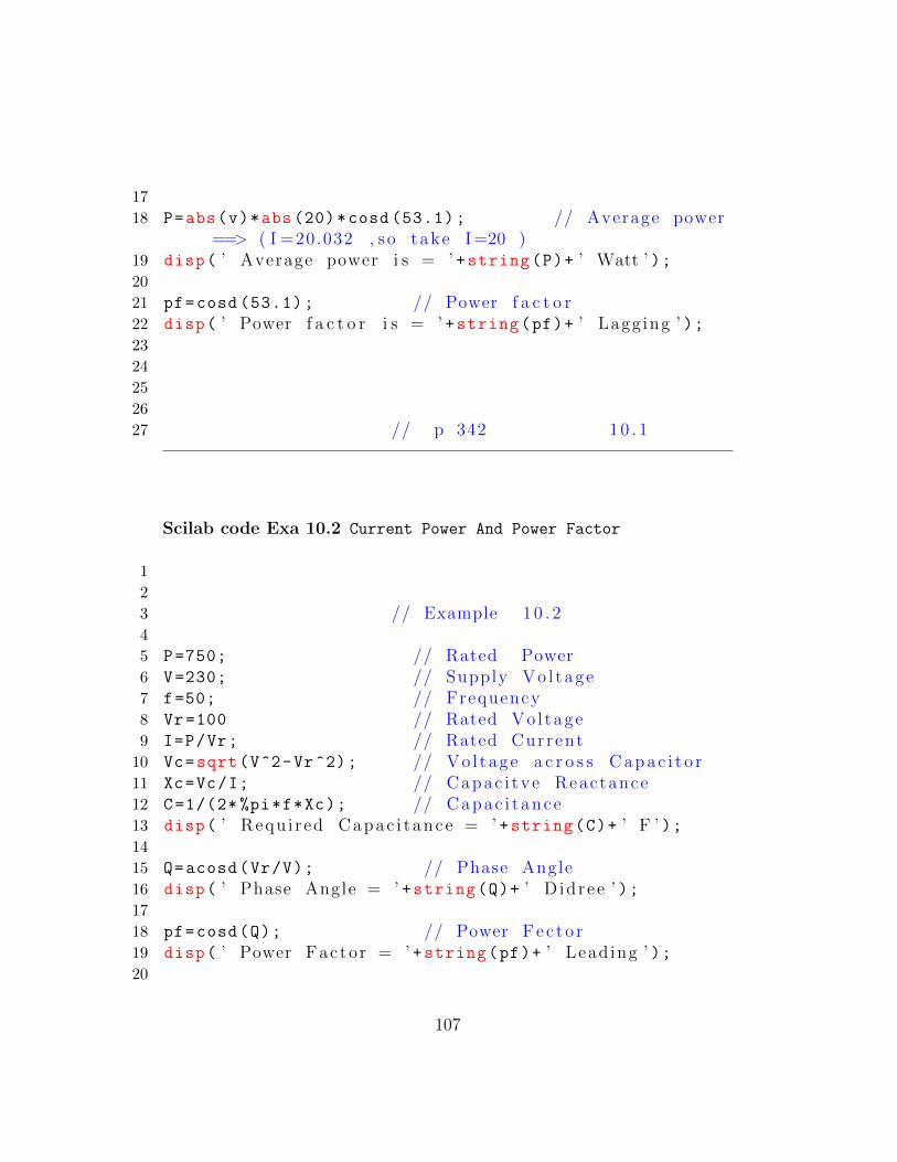
17
18 P=abs(v)*abs (20)*cosd (53.1); // Average power==> ( I =20.032 , so take I =20 )
19 disp( ’ Average power i s = ’ +string(P)+ ’ Watt ’ );20
21 pf=cosd (53.1); // Power f a c t o r22 disp( ’ Power f a c t o r i s = ’ +string(pf)+ ’ Lagg ing ’ );23
24
25
26
27 // p 342 1 0 . 1
Scilab code Exa 10.2 Current Power And Power Factor
1
2
3 // Example 1 0 . 24
5 P=750; // Rated Power6 V=230; // Supply Vo l tage7 f=50; // Frequency8 Vr=100 // Rated Vo l tage9 I=P/Vr; // Rated Current
10 Vc=sqrt(V^2-Vr^2); // Vo l tage a c r o s s C a p a c i t o r11 Xc=Vc/I; // Capac i tve Reactance12 C=1/(2* %pi*f*Xc); // Capac i t ance13 disp( ’ Requ i red Capac i tance = ’ +string(C)+ ’ F ’ );14
15 Q=acosd(Vr/V); // Phase Angle16 disp( ’ Phase Angle = ’ +string(Q)+ ’ D idree ’ );17
18 pf=cosd(Q); // Power Fec to r19 disp( ’ Power Facto r = ’ +string(pf)+ ’ Lead ing ’ );20
107

21 Pa=V*I; // Apparent power22 disp( ’ Apparent v a l u e o f Power = ’ +string(Pa)+ ’ VA ’ )
;
23
24 Pr=V*I*sind(Q); // R e a c t i v e Power25 disp( ’ R e a c t i v e Power = ’ +string(round(Pr))+ ’ VAR ’ );26
27
28
29 // p 344 1 0 . 2
Scilab code Exa 10.3 Resistance Voltage And Power
1
2
3 // Example 1 0 . 34
5 R=120; // R e s i s t a n c e6 Xc=250; // Capac i tve Reactance7 Q= -64.4; // Phase Angle8 I=0.9+ %i*0; // Current9 Z=R-%i*Xc; // Impedance
10 disp( ’ The Impedance i s = ’ +string(Z)+ ’ o r ( ’ +string(abs(Z))+ ’ < ’ +string(atand(imag(Z),real(Z)))+ ’ Amp ) ’ );
11
12 pf=cosd(Q); // Power Fec to r13 disp( ’ Power Facto r = ’ +string(pf)+ ’ Lead ing ’ );14
15 V=I*Z; // Supply Vo l tage16 disp( ’ Supply Vo l tage = ’ +string(V)+ ’ o r ( ’ +string
(abs(V))+ ’ < ’ +string(atand(imag(V),real(V)))+ ’Amp ) ’ );
17 v=249.6; // Peak v a l u e o f Vo l tage18
108

19 Vr=I*R; // Vo l tage at R e s i s t o r20 disp( ’ Vo l tage a c r o s s R e s i s t o r = ’ +string(Vr)+ ’ Vo l t
’ );21
22 Vc=I*Xc; // Vo l tage a c r o s sC a p ac i t o r
23 disp( ’ Vo l tage a c r o s s C ap a c i t o r = ’ +string(Vc)+ ’ o r( ’ +string(abs(Vc))+ ’ < −90 Amp ) ’ );
24 Pa=v*I; // Apparent power25 disp( ’ Apparent v a l u e o f Power = ’ +string(Pa)+ ’ VA ’ )
;
26
27 Pac=v*I*cosd(Q); // Act i v e Power28 disp( ’ Ac t i v e Power = ’ +string(Pac)+ ’ Watt ’ );29
30 Pr=v*I*sind(Q); // R e a c t i v e Power31 disp( ’ R e a c t i v e Power = ’ +string(-Pr)+ ’ VAR ’ );32
33
34
35 // p 345 1 0 . 3
Scilab code Exa 10.4 Resistance Power And Power Factor
1
2
3 // Example 1 0 . 44
5 // Given V= 160+ i 1 2 0 & I= −4+i 1 0
6 Vi= 160+%i *120; // S i n u s o i d a l Vo l tage i . e200 <36.87
7 Ii= -4+%i*10; // S i n u s o i d a l Current i . e10 .77 <111 .8
8 Z=Vi/Ii; // Impedance
109
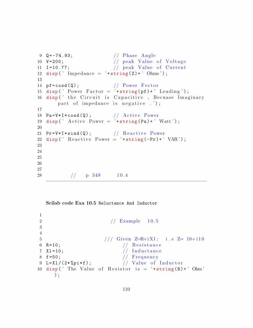
9 Q= -74.93; // Phase Angle10 V=200; // peak Value o f Vo l tage11 I=10.77; // peak Value o f Current12 disp( ’ Impedance = ’ +string(Z)+ ’ Ohms ’ );13
14 pf=cosd(Q); // Power Fec to r15 disp( ’ Power Facto r = ’ +string(pf)+ ’ Lead ing ’ );16 disp( ’ the C i r c u i t i s C a p a c i t i v e , Becuase Imag inary
pa r t o f impedance i s n e g a t i v e . ’ );17
18 Pa=V*I*cosd(Q); // Act i v e Power19 disp( ’ Ac t i v e Power = ’ +string(Pa)+ ’ Watt ’ );20
21 Pr=V*I*sind(Q); // R e a c t i v e Power22 disp( ’ R e a c t i v e Power = ’ +string(-Pr)+ ’ VAR ’ );23
24
25
26
27
28 // p 348 1 0 . 4
Scilab code Exa 10.5 Reluctance And Inductor
1
2 // Example 1 0 . 53
4
5 // / Given Z=R+i X l ; i . e Z= 10+ i 1 06 R=10; // R e s i s t a n c e7 Xl=10; // Induc tance8 f=50; // Frequency9 L=Xl/(2* %pi*f); // Value o f I n d u c t o r
10 disp( ’ The Value o f R e s i s t o r i s = ’ +string(R)+ ’ Ohm ’);
110

11 disp( ’ The Value o f I n d u c t o r i s = ’ +string(L)+ ’ H ’ );12
13
14
15 // p 348 1 0 . 5
Scilab code Exa 10.6 Resistance And Capacitor
1
2 // Example 1 0 . 63
4 // Given Z=R+iX ; i . e Z= 10− i 1 05
6 R1=10; // R e s i s t a n c e7 Xl=10; // Induc tance8 f=50; // Frequency9 Z= 10-%i*10; // Impedance
10 Y=1/Z; // Admitance11 disp( ’ The Admitance o f C i r c u i t i s = ’ +string(Y)+ ’ S
’ );12 G=0.05; // he r e G=1/R13 B=0.05; // he r e B= 1/C14 R=1/G; // R e s i s t a n c e15 disp( ’ The R e s i s t a n c e o f C i r c u i t i s = ’ +string(R)+ ’
Ohm ’ );16
17 C=B/(2* %pi*f); // Capac i t ance18 disp( ’ The Capac i t ance o f C i r c u i t i s = ’ +string(C)+ ’
F ’ );19
20
21
22 // p 348 1 0 . 6
111
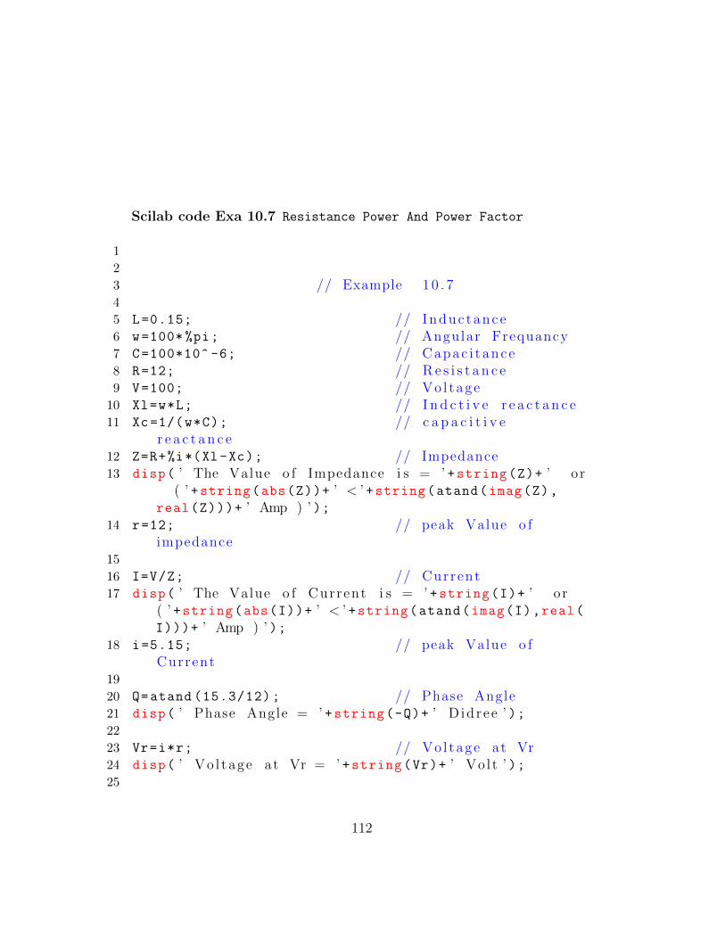
Scilab code Exa 10.7 Resistance Power And Power Factor
1
2
3 // Example 1 0 . 74
5 L=0.15; // Induc tance6 w=100* %pi; // Angular Frequancy7 C=100*10^ -6; // Capac i t ance8 R=12; // R e s i s t a n c e9 V=100; // Vo l tage
10 Xl=w*L; // I n d c t i v e r e a c t a n c e11 Xc=1/(w*C); // c a p a c i t i v e
r e a c t a n c e12 Z=R+%i*(Xl-Xc); // Impedance13 disp( ’ The Value o f Impedance i s = ’ +string(Z)+ ’ o r
( ’ +string(abs(Z))+ ’ < ’ +string(atand(imag(Z),real(Z)))+ ’ Amp ) ’ );
14 r=12; // peak Value o fimpedance
15
16 I=V/Z; // Current17 disp( ’ The Value o f Current i s = ’ +string(I)+ ’ o r
( ’ +string(abs(I))+ ’ < ’ +string(atand(imag(I),real(I)))+ ’ Amp ) ’ );
18 i=5.15; // peak Value o fCurrent
19
20 Q=atand (15.3/12); // Phase Angle21 disp( ’ Phase Angle = ’ +string(-Q)+ ’ D idree ’ );22
23 Vr=i*r; // Vo l tage at Vr24 disp( ’ Vo l tage at Vr = ’ +string(Vr)+ ’ Vo l t ’ );25
112
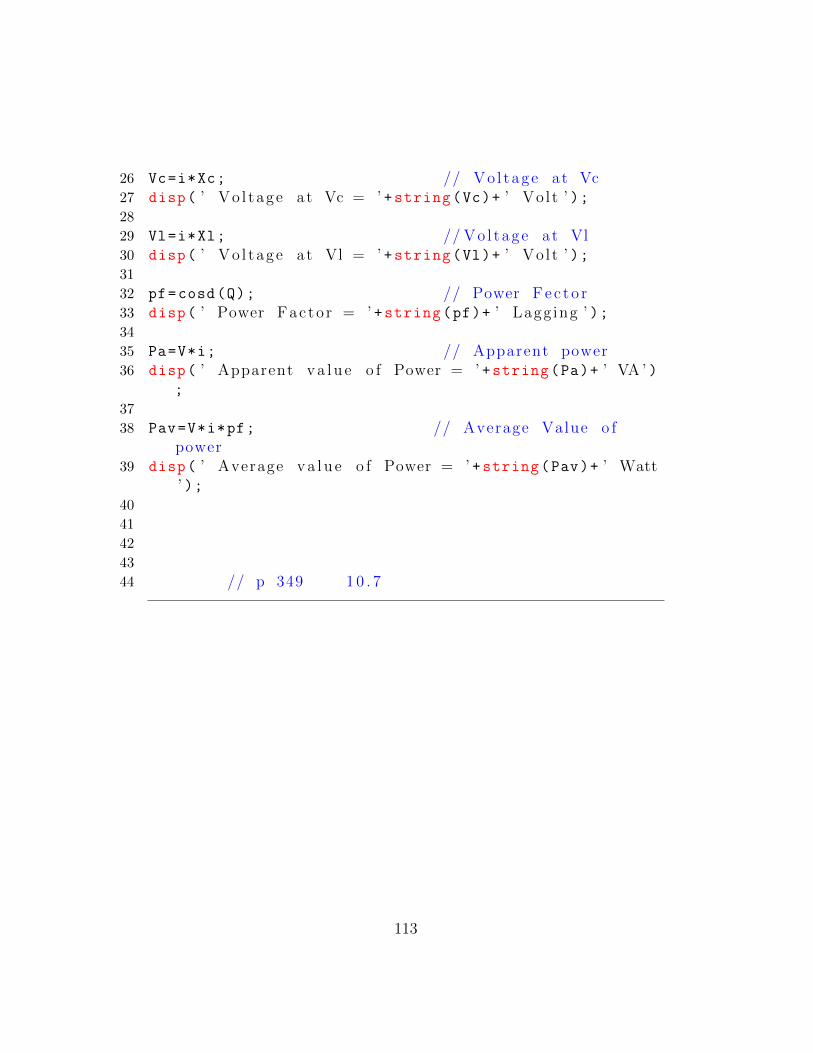
26 Vc=i*Xc; // Vo l tage at Vc27 disp( ’ Vo l tage at Vc = ’ +string(Vc)+ ’ Vo l t ’ );28
29 Vl=i*Xl; // Vo l tage at Vl30 disp( ’ Vo l tage at Vl = ’ +string(Vl)+ ’ Vo l t ’ );31
32 pf=cosd(Q); // Power Fec to r33 disp( ’ Power Facto r = ’ +string(pf)+ ’ Lagg ing ’ );34
35 Pa=V*i; // Apparent power36 disp( ’ Apparent v a l u e o f Power = ’ +string(Pa)+ ’ VA ’ )
;
37
38 Pav=V*i*pf; // Average Value o fpower
39 disp( ’ Average v a l u e o f Power = ’ +string(Pav)+ ’ Watt’ );
40
41
42
43
44 // p 349 1 0 . 7
113

Chapter 11
Resonance in AC Circuits
Scilab code Exa 11.1 Frequence And Voltage
1
2 // Example 1 1 . 13
4 L=0.15; // I n d u c t o r5 C=100*10^ -6; // C a p ac i t o r6 fo =1/{2* %pi*sqrt(L*C)}; // Resonance f r e q u e n c y7 disp( ’ Resonance f r e q u e n c y ( f o ) = ’ +string(fo)+ ’ Hz ’
);
8
9 R=12; // C i r c u i t r e s i s t a n c e10 V=100; // Source v o l t a g e11 Io=V/R; // Maximum c u r r e n t by
s o u r c e12 disp( ’ Maximum c u r r e n t by s o u r c e = ’ +string(Io)+ ’
Amp ’ );13
14 r1=R^2/(2*L^2); // f o r ea syc a l c u l a t i o n
15 r2=(1/(L*C)); // f o r ea syc a l c u l a t i o n
16 fc =(1/6.28)*sqrt(r2-r1); // Frequency f o r
114
maximum c a p a c i t o r v o l t a g e17 disp( ’ Frequency f o r maximum c a p a c i t o r v o l t a g e = ’ +
string(fc)+ ’ Hz ’ );18
19
20 r3=(R^2*C^2)/2; // f o r ea syc a l c u l a t i o n
21 fl =1/{2* %pi*sqrt((L*C)-r3)}; // Frequency f o rmaximum c a p a c i t o r v o l t a g e
22 disp( ’ Frequency f o r maximum c a p a c i t o r v o l t a g e = ’ +string(fo)+ ’ Hz ’ );
23
24 Xl=2*%pi*fo*L; // I n d u c t i v er e a c t a n c e
25 disp( ’ I n d u c t i v e r e a c t a n c e = ’ +string(Xl)+ ’ Ohms ’ );26
27 Xc =1/(2* %pi*fo*C); // I n d u c t i v e r e a c t a n c e28 disp( ’ C a p a c i t i v e r e a c t a n c e = ’ +string(Xc)+ ’ Ohms ’ );29
30 Q=Xl/R; // Qua l i t y f a c t o r31 disp( ’ Qua l i t y f a c t o r = ’ +string(Q));32
33 VLC=Q*V; // Vo l tage drop a c r o s sthe e l e m e n t s
34 disp( ’ Vo l tage drop a c r o s s the e l e m e n t s = ’ +string(VLC)+ ’ Vo l t ’ );
35
36
37
38 // p 378 1 1 . 1
Scilab code Exa 11.2 Capacitor Voltage And Q FActor
1
2 // Example 1 1 . 2
115

3
4 L=0.5; // Induc tance5 V=100; // Supply Vo l tage6 R=4; // R e s i s t a n c e7 f=50; // Frequency8 C=1/(4* %pi ^2*f^2*L); // Capac i t ance9 disp( ’ Capac i t ance i s = ’ +string(C*10^6)+ ’ uF ’ );10
11 I=V/R; // Current at ResonanceFrequency
12 disp( ’ Current at Resonance Frequency = ’ +string(I)+’ Amp ’ );
13
14 wo=2*%pi*f; // Angular Frequency15 Xl=157; // I n d c t i v e Reactance16 Vc=I*Xl; // Vo l tage a c r o s s
C a p ac i t o r17 disp( ’ Vo l tage a c r o s s C ap a c i t o r = ’ +string(Vc)+ ’
Vo l t ’ );18
19 Vl=Vc; // Vo l tage a c r o s sInduc tance
20 disp( ’ Vo l tage a c r o s s Induc tance = ’ +string(Vl)+ ’Vo l t ’ );
21
22
23 Q=(wo*L)/R; // Q−Facto r24 disp( ’ Q−Facto r i s = ’ +string(Q));25
26
27
28
29
30 // p 378 1 1 . 2
116
Scilab code Exa 11.3 Inductor Current And Voltage
1
2 // Example 1 1 . 33
4
5 V=0.85; // Supply Vo l tage6 f=175*10^3; // Frequency7 C=320*10^ -12; // Capac i t ance8
9 L=1/(4*3.14^2*f^2*C); // Induc tance10 disp( ’ I nduc tance i s = ’ +string(L*10^3)+ ’ mH’ );11
12 Xl =2*3.14*f*L; // I n d c t i v e r e a c t a n c e13 Q=50; // Q−Facto r14 R=Xl/Q; // R e s i s t a n c e15
16 I=V/R; // c i r c u i t c u r r e n t17 disp( ’ C i r c u i t c u r r e n t i s = ’ +string(I*1000)+ ’ mA’ );18
19 Vc=Q*V; // Vo l tage a c r o s sC a p ac i t o r
20 disp( ’ Vo l tage a c r o s s C ap a c i t o r = ’ +string(Vc)+ ’Vo l t ’ );
21
22
23
24
25 // p379 1 1 . 3
Scilab code Exa 11.4 Capacitor Current And Enegy
1
2 // Example 1 1 . 43
117
4 L=1*10^ -3; // Induc tance5 V=120; // Supply Vo l tage6 R=2; // R e s i s t a n c e7 f=5*10^3; // Frequency8 C=1/(4* %pi ^2*f^2*L); // Capac i t ance9 disp( ’ Capac i t ance i s = ’ +string(C*10^9)+ ’ nF ’ );10
11 I=V/R; // Current at ResonanceFrequency
12 disp( ’ Current at Resonance Frequency = ’ +string(I)+’ Amp ’ );
13
14 Emax=L*I^2; // Maximum I n s t a n t a n e o u sEnergy
15 disp( ’ The Maximum I n s t a n t a n e o u s Energy = ’ +string(Emax)+ ’ J ’ );
16
17
18
19
20
21 // p 379 1 1 . 4
Scilab code Exa 11.5 Frequence And Q Factor
1
2
3 // Example 1 1 . 54
5 R1 =0.51; // R e s i s t a n c e −16 R2=1.3; // R e s i s t a n c e −27 R3 =0.24; // R e s i s t a n c e −38 Req=R1+R2+R3; // E q v i u a l e n t
R e s i s t a n c e9 L1=32*10^ -3; // Inductance −1
118
10 L2=15*10^ -3; // Inductance −211 Leq=L1+L2; // E q v i u a l e n t
Induc tance12 C1=62*10^ -6; // Capac i tance−113 C2=25*10^ -6; // Capac i tance−214 Ceq=(C1*C2)/(C1+C2); // E q v i u a l e n t
Capac i t ance15
16 fo =1/(2* %pi*sqrt(Leq*Ceq)); // ResonanceFrequency
17 disp( ’ Resonance Frequency i s = ’ +string(round(fo))+’ Hz ’ );
18
19 Q=(1/ Req)*sqrt(Leq/Ceq); // Over a l l Q−Facto r
20 disp( ’ Over a l l Q−Facto r i s = ’ +string(round(Q)));21
22 wo=2*%pi*fo;
23 Q1=(wo*L1)/R1; // Q−Facto r o fCo i l−1
24 disp( ’ Q−Facto r o f Co i l−1 i s = ’ +string(Q1));25
26 Q2=(wo*L2)/R2; // Q−Facto r o f Co i l−2
27 disp( ’ Q−Facto r o f Co i l−2 i s = ’ +string(Q2));28
29
30
31
32 // p 380 1 1 . 5
Scilab code Exa 11.6 Frequence
1
2 // Example 1 1 . 6
119
3
4 f=150*10^3; // Frequency5 Bw =75*10^3; // Band width6 Q=f/Bw; // Q−Facto r7 disp( ’ Q−Facto r i s = ’ +string(Q));8 // s i n c e Q < 10 t h e r e f o r we need
to s o l v e by Equat ion9 // 75= f2−f 1 & 150= r o o t ( f 1 ∗ f 2 )10 // w i l l g e t Eq ( f 1 ˆ2+ 75 f1− 22500= 0
) by E l i m i n a t i n g f 211 // by f a c t o r i z a t i o n we have f 1 =(
1 1 7 . 1 kHz or −192.1kHz )12 f1 =117.1;
13 f2=75+f1;
14 disp( ’ The h a l f Power F r e q u e n c i e s a r e f 1= ’ +string(f1)+ ’ kHz & f 2= ’ +string(f2)+ ’ kHz ’ );
15
16
17
18 // p 382 1 1 . 6
Scilab code Exa 11.7 Resistance Current And Capacitor
1
2 // Example 1 1 . 73
4 V=230; // Supply Vo l tage5 L=200*10^ -6; // Induc tance6 R=20; // R e s i s t a n c e7 f=1*10^6; // Frequency8 Xl=2*%pi*f*L; // I n d c t i v e r e a c t a n c e9 C=1/(4* %pi ^2*f^2*L); // Capac i t ance
10 disp( ’ Requ i red Capac i tance = ’ +string(C*10^12)+ ’ pF’ );
11
120

12 Q=Xl/R; // Q−Facto r13 disp( ’ Q−Facto r i s = ’ +string(Q));14
15 Zo=L/(C*R); // dynamic Impedance16 disp( ’ Dynamic Impedance i s = ’ +string(Zo)+ ’ Ohm ’ );17 Zs =8000; // Soure s R e s i s t a n c e18 Z=Zo+Zs; // Tota l R e s i s t a n c e19
20 I=V/Z; // Tota l L ine Current21 disp( ’ Tota l L ine Current i s = ’ +string(I*1000)+ ’ mA
’ );22
23
24
25 // p 388 1 1 . 7
Scilab code Exa 11.8 Frequence And Q Factor
1
2
3 // Example 1 1 . 84
5 L=0.24; // Induc tance6 C=3*10^ -6; // Capac i t ance7 R=150; // R e s i s t a n c e8 f=1/(2* %pi*sqrt(L*C)); // Frequency9 fo=f*sqrt(1-R^2*(C/L)); // Resonance Frequency
10 disp( ’ Resonance Frequency = ’ +string(fo)+ ’ Hz ’ );11
12 Xl=2*%pi*fo*L; // I n d c t i v e r e a c t a n c e13 Q=Xl/R; // Q−Facto r14 disp( ’ Q−Facto r i s = ’ +string(Q));15
16 Bw=fo/Q; // Band width17 disp( ’ Band width i s = ’ +string(Bw)+ ’ Hz ’ );
121
18
19
20
21
22 // p 387 1 1 . 8
122
Chapter 12
Three Phase Circuits AndSystem
Scilab code Exa 12.1 Current
1
2 // Example 1 2 . 13
4 // Given Z= 32+ i 2 45 R=32; // Real Part o f Z6 X=24; // Imag inary Part o f Z7 z=R+%i*X; // Impedance8 Z=abs(z); // Abso lu te v a l u e o f Z9 Vl=400; // Supply Vo l tage
10 Vph1=Vl /1.732; // Vo l tage i n Y−Connect ion11 Iph1=Vph1/Z; // Current i n Y−Connect ion12 Il1=Iph1; // Load Current i n Y−
Connect ion13 disp( ’ Current Drawn ( f o r Y−Connect ion ) = ’ +string
(Il1)+ ’ Amp ’ );14 Vph2=Vl; // Vo l tage i n Delta−Connect ion15 Iph2=Vph2/Z; // Current i n Delta−Connect ion16 Il2 =1.732* Iph2; // Load Current i n Delta−
Connect ion
123
17 disp( ’ Current Drawn ( f o r Delta−Connect ion ) = ’ +string(Il2)+ ’ Amp ’ );
18
19
20
21
22 // p 409 1 2 . 1
Scilab code Exa 12.2 Current
1
2
3 // Example 1 2 . 24
5 Vl=415; // Supply Vo l tage6 Vph=Vl/sqrt (3); // Phase Vo l tage7 p1 =10000; // Load o f 10−kW8 p2 =8000; // Load o f 8−kW9 p3 =5000; // Load o f 5−kW10
11 IR=p1/Vph; // Current by ( 10−kW Load )12 disp( ’ Current by ( 10−kW Load ) = ’ +string(IR)+ ’
Amp ’ );13
14 IY=p2/Vph; // Current by ( 8−kW Load )15 disp( ’ Current by ( 8−kW Load ) = ’ +string(IY)+ ’ Amp
’ );16
17 IB=p3/Vph; // nCurrent by ( 5−kW Load )18 disp( ’ Current by ( 5−kW Load ) = ’ +string(IB)+ ’ Amp
’ );19
20 IH=IY*cosd (30)-IB*cosd (30); // H o r i z o n t a lCurrent
21 IV=IR-IY*sind (30)-IB*sind (30); // V e r t i c a l
124
Current22 IN=sqrt(IH^2+IV^2); // Current i n
Neut ra l Conductor23 disp( ’ Current i n Neut ra l Conductor = ’ +string(IN)+ ’
Amp ’ );24
25
26
27
28 // p 410 1 2 . 2
Scilab code Exa 12.3 Current
1
2 // Example 1 2 . 33
4 Z1=100; // Impedence Z1 i n Delta−c o n n e c t i o n l oad
5 R2=20; // R e s i s t a n c e R2 i n Delta−c o n n e c t i o n l oad
6 f=50; // Frequency7 L2 =0.191; // Induc tance8 X2=2*%pi*f*L2; // Reactance X2 i n Delta−
c o n n e c t i o n l oad9 Z2=sqrt(R2^2+X2^2); // Impedence Z2 i n Delta−
c o n n e c t i o n l oad10 Q2=atand (60/20); // Phase a n g l e11 C3=30*10^ -6; // C a p ac i t o r12 Z3 =1/(2* %pi*f*C3); // Impedence Z3 i n Delta−
c o n n e c t i o n l oad13 Q3=90; // Leading phase a n g l e14 I1=415/Z1; // Phase c u r r e n t I1 i n l o a d s RY15 disp( ’ Phase c u r r e n t I1 i n l o a d s RY = ’ +string(I1)+ ’
Amp ’ );16
125
17 I2=415/Z2; // Phase c u r r e n t I2 i n l o a d s YB18 disp( ’ Phase c u r r e n t I2 i n l o a d s YB = ’ +string(I2)+ ’
Amp ’ );19
20 I3=415/Z3; // Phase c u r r e n t I3 i n l o a d s BR21 disp( ’ Phase c u r r e n t I3 i n l o a d s BR = ’ +string(I3)+ ’
Amp ’ );22
23 IR=sqrt(I1^2+I3 ^2+(2* I1*I3*cosd (30))); //Current i n the l i n e r conduc to r R
24 disp( ’ Current i n the l i n e r conduc to r R = ’ +string(IR)+ ’ Amp ’ );
25
26 QY=Q2 -60; // Phase d i f f r e n c e between I2−I 1
27 IY=sqrt(I1^2+I2 ^2+(2* I1*I2*cosd(QY))); //Current i n the l i n e r conduc to r Y
28 disp( ’ Current i n the l i n e r conduc to r Y = ’ +string(IY)+ ’ Amp ’ );
29
30 QB=180-QY -30; // Phase d i f f r e n c e between I2−I 3
31 IB=sqrt(I2^2+I3 ^2+(2* I2*I3*cosd(QB))); //Current i n the l i n e r conduc to r B
32 disp( ’ Current i n the l i n e r conduc to r B = ’ +string(IB)+ ’ Amp ’ );
33
34
35
36
37 // p 411 1 2 . 3
Scilab code Exa 12.4 Current Power And Power Factor
1
126
2 // Example 1 2 . 43
4 // ==> For s t a r−c o n n e c t i o n5 disp( ’ ∗∗ For s t a r−c o n n e c t i o n ∗∗ ’ );6 Vl=400; // Vo l tage at l oad7 Vph=Vl /1.732; // Phase v o l t a g e8 Zph=sqrt (20^2+15^2); // Impedence per phase9 Il=Vph/Zph; // Line c u r r e n t10 disp( ’ The l i n e c u r r e n t ( I l ) = ’ +string(Il)+ ’ Amp ’ );11
12 Rph =20; // R e s i s t a n c e per phase13 CosQ=Rph/Zph; // Power f a c t o r14 disp( ’ Power f a c t o r = ’ +string(CosQ)+ ’ Lagg ing ’ );15
16 P=1.732* Vl*Il*CosQ; // Tota l a c t i v e power17 disp( ’ Tota l a c t i v e power = ’ +string(P/1000)+ ’ kW’ );18
19 // ==> For Delta−c o n n e c t i o n20 disp( ’ ∗∗ For Delta−c o n n e c t i o n ∗∗ ’ );21 Vph1=Vl; // Phase v o l t a g e22 Iph=Vph1/Zph; // Phase c u r r e n t23 IL =1.732* Iph; // Load c u r r e n t24 disp( ’ The Load c u r r e n t ( IL ) = ’ +string(IL)+ ’ Amp ’ );25
26 disp( ’ Power f a c t o r = ’ +string(CosQ)+ ’ Lagg ing ’ );27
28 P1 =1.732* Vl*IL*CosQ; // Tota l a c t i v e power29 disp( ’ Tota l a c t i v e power = ’ +string(P1 /1000)+ ’ kW’ )
;
30
31
32 // p 412 1 2 . 4
Scilab code Exa 12.5 Power And Power Factor
127
1
2 // Example 1 2 . 53
4 p1 =3000; // Load o f 3−kW5 p2 =1500; // Load o f 1.5−
kW6 P=p1+p2; // Tota l Load7 disp( ’ Tota l Power Consumed = ’ +string(P)+ ’ Watt ’ );8
9 Q=atand (1.732*(p1-p2)/(p1+p2)); // Power Facto rAngle
10 pf=cosd(Q); // Power Facto r11 disp( ’ Power Facto r i s = ’ +string(pf));12
13
14
15
16 // p 417 1 2 . 5
Scilab code Exa 12.6 Current Power And Power Factor
1
2 // Example 1 2 . 63
4 Vl=415 // SupplyVo l tage
5 p1 =5200; // Load o f 5.2−kW
6 p2= -1700; // Load o f 1.7−kW
7
8 P=p1+p2; // Tota l Load9 disp( ’ Tota l Power Consumed = ’ +string(P)+ ’ Watt ’ );10
11 Q=atand (1.732*(p1-p2)/(p1+p2)); // Power Facto r
128
Angle12
13 pf=cosd(Q); // Power Facto r14 disp( ’ Power Facto r i s = ’ +string(pf));15
16 // P= r o o t ( 3 ) ∗Vl∗ I l ∗Cos (Q)
17 Il=P/(1.732* Vl*pf);
18 disp( ’ L ine Current i s = ’ +string(Il)+ ’ Amp ’ );19
20
21
22
23 // p 417 1 2 . 6
129
Chapter 13
Transformers
Scilab code Exa 13.1 Megnetic Flux And Voltage
1
2
3 // Example 1 3 . 14
5 E=6400; // Supply Vo l tage6 f=50; // Frequency7 N1=480; // No . Of t u r n s i n
Primary C o i l8 N2=20; // No . Of t u r n s i n
Secondary C o i l9
10 Qm=E/(4.44*f*N1); // The Peak Valueo f Flux
11 disp( ’ The Peak Value o f Flux = ’ +string(Qm)+ ’ Wb’ );12
13 E1 =4.44*f*N2*Qm; // Vo l tageinduced i n Secondary wind ing
14 disp( ’ Vo l tage induced i n Secondary winding = ’ +string(E1)+ ’ Vo l t ’ );
15
16
130
17
18
19
20
21 // p 487 1 3 . 1
Scilab code Exa 13.2 Flux Density Current And Voltage
1
2 // Example 1 3 . 23
4 E1=230; // Supply Vo l tage5 f=50; // Frequency6 N1=30; // No . Of t u r n s i n
Primary C o i l7 N2=350; // No . Of t u r n s i n
Secondary C o i l8 A=250*10^ -4; // Area o f the
Core9
10 Qm=E1 /(4.44*f*N1); // The Peak Valueo f Flux
11 Bm=Qm/A; // The Peak Valueo f Flux Dens i ty
12 disp( ’ The Peak Value o f Flux Dens i ty = ’ +string(Bm)+ ’ Te s l a ’ );
13
14 E2=E1*(N2/N1); // Vo l tageinduced i n Secondary wind ing
15 disp( ’ Vo l tage induced i n Secondary winding = ’ +string(E2 /1000)+ ’ kV ’ );
16
17 I2=100; // Current i nSecondary C o i l
18 I1=I2*(N2/N1); // Primary
131
Current19 disp( ’ Primary Current i s = ’ +string(I1 /1000)+ ’ kA ’
);
20
21
22
23
24 // p 490 1 3 . 2
Scilab code Exa 13.3 Turns Ratio
1
2
3 // Example 1 3 . 34
5 Rl=800; // Load R e s i s t a n c e6 Req =50; // O/P R e s i s t a n c e7 K=sqrt(Rl/Req); // Rat io Constant8 N21=K; // urns r a t i o o f
Trans fo rmer9 disp( ’ Turns r a t i o o f Trans fo rmer (N2/N1) = ’ +string
(N21));
10
11
12
13
14
15 // p 490 1 3 . 3
Scilab code Exa 13.4 Current
1
2 // Example 1 3 . 4 ’
132
3
4 // From the c i r c u i t Diagram Ip=30<0/{20+ i 2 0 +2ˆ2∗(2− i 1 0 ) }
5
6 Ip= 30/{20+ %i *20+2^2*(2 - %i*10)}; // Phase Current7
8 Il=2*Ip; // Load c u r r e n t9 disp( ’ The Load c u r r e n t i s I l = ’ +string(Il)+ ’ Amp
or ( ’ +string(abs(Il))+ ’ < ’ +string(atand(imag(Il),real(Il)))+ ’ Amp ) ’ );
10
11
12
13
14
15
16
17 // p 491 1 3 . 4
Scilab code Exa 13.5 Power
1
2 // Example 1 3 . 53
4 f=50; // Frequency5 N1=30; // No . Of t u r n s i n
Primary C o i l6 N2=66; // No . Of t u r n s i n
Secondary C o i l7 A=0.015; // Area o f the
Core8 Zl=4; // Load Impedance9 Bm=1.1; // The Peak Value
o f Flux Dens i ty10 Qm=Bm*A; // The Peak Value
133
o f Flux11
12 V2 =4.44*f*N2*Qm; // O/P Vo l tage13 I2=V2/Zl; // O/P c u r r e n t14 Ova=V2*I2; // Output Volt−
Amperes15 disp( ’ Output Volt−Amperes i s = ’ +string(Ova /1000)+ ’
kVA ’ );16
17
18
19
20
21 // p 491 1 3 . 5
Scilab code Exa 13.6 Turns
1
2 // Example 1 3 . 63
4 f=50; // Frequency5 A=9*10^ -4; // Area o f the
Core6 Bm=1; // The Peak Value
o f Flux Dens i ty7 Qm=Bm*A; // The Peak Value
o f Flux8
9 E3=6; // Vo l tage i nT e r t i a r y wind ing
10 N3=E3 /(4.44*f*Qm); // No . Of Turns i nT e r t i a r y wind ing
11 disp( ’ No . Of Turns i n T e r t i a r y wind ing = ’ +string(round(N3*2)) + ’ t u r n s ’ );
12
134
13
14 E1=230; // Vo l tage i nPrimary winding
15 N03=round(N3); // Round f i g u r e16 N1=(N03*E1)/E3; // No . Of Turns
i n Primary wind ing17 disp( ’ No . Of Turns i n Primary wind ing = ’ +string(
round(N1)) + ’ t u r n s ’ );18
19
20 E1=230;
21 E2=110; // Vo l tage i nSecondary wind ing
22 N2=(N03*E2)/E3; // No . Of Turnsi n Secondary winding
23 disp( ’ No . Of Turns i n Secondary wind ing = ’ +string(round(N2)) + ’ t u r n s ’ );
24
25
26
27
28
29 // p 491 1 3 . 6
Scilab code Exa 13.7 Current And Power Factor
1
2
3 // Example 1 3 . 74
5 VA=350; // VA r a t i n g6 V1=230; // I /p Vo l tage7 Io=VA/V1; // I /p Current8 Pi=110; // I /p power9 // Core Loss = I /p power at
135

no l oad10 // Pi= V1∗ I o ∗CosQ11 pf=Pi/VA; // Power f a c t o r12 disp( ’ Power f a c t o r at no l aod = ’ +string(pf));13
14 Iw=Io*pf; // Loss component o f no−l o adCurrent
15 disp( ’ Loss component o f no−l o ad Current = ’ +string(Iw)+ ’ Amp ’ );
16
17 Im=sqrt(Io^2-Iw^2); // Magne t i s i ng component o fno−l o ad Current
18 disp( ’ Magne t i s i ng component o f no−l o ad Current = ’ +string(Im)+ ’ Amp ’ );
19
20
21
22 // p 493 1 3 . 7
Scilab code Exa 13.8 Power
1
2
3 // Example 1 3 . 84
5 // We Know tha t Pi= Ph+ Pe=(Af+ Bf ˆ2 )
6 // t h e r e f o r at 60Hz 100=60A+ 3600B
7 // at 40Hz 60 =40A+ 1600B
8 // A f t e r S o l v i n g Equat ion Wehave
9 A=1.167; // Alphabet f o r S i m l i c i t y10 B=0.00834; // Alphabet f o r S i m l i c i t y
136
11 f=50; // Frequency12 Ph=A*f; // H y s t e r e s i s Loss13 disp( ’ H y s t e r e s i s Loss ( at 50 Hz ) = ’ +string(Ph)+ ’
Watt ’ );14
15 Pe=B*f^2; // Eddy−Current Loss16 disp( ’ Eddy−Current Loss ( at 50 Hz ) = ’ +string(Pe)+
’ Watt ’ );17
18
19
20
21
22
23 // p 495 1 3 . 8
Scilab code Exa 13.9 Current And Power Factor
1
2 // Example 1 3 . 93
4 pf1 =0.2; // Power f a c t o r at 5 A5 pf2 =0.8; // Power f a c t o r at 120 A6 Q1=acosd(pf1); // Angle f o r 0 . 2 Power f a c t o r7 Q2=acosd(pf2); // Angle f o r 0 . 8 Power f a c t o r8 V2=110; // Vo l tage i n Secondary
wind ing9 V1=440; // Vo l tage i n Primary wind ing10 k=V2/V1; // Rat io Constant11 I2=120; // Current i n Secondary
wind ing12 i1=k*I2; // Current i n pr imary winding13 io=5; // No load Current14 I1=23.99 -%i*18; // Current i n pr imary winding
i n complex form
137
15 Io=1-%i *4.899; // No load Current i n complexform
16
17 I=I1+Io; // Primary Current18 disp( ’ Primary Current = ’ +string(I)+ ’ Amp or ’ +
string(abs(I))+ ’< ’ +string(atand(imag(I),real(I)))+ ’ Amp ’ );
19
20 pf=cosd ( -42.49); // Primary Power f a c t o r21 disp( ’ Primary Power f a c t o r = ’ +string(pf));22
23
24
25
26 // / p 498 1 3 . 9
Scilab code Exa 13.10 Resistance And Power
1
2 // Example 1 3 . 1 03
4 kVA =50000; // S i n g l e Phase supp ly5 V1 =4400; // Vo l tage i n pr imary winding6 V2=220; // Vo l tage i n Secondary
wind ing7 R1 =3.45; // pr imary R e s i s t a n c e8 R2 =0.009; // Secondary R e s i s t a n c e9 X1=5.2; // pr imary Reactance10 X2 =0.015; // Secondary Reactance11 I1=kVA/V1; // pr imary Current12 I2=kVA/V2; // Secondary Current13 k=V2/V1; // Turns c o n s t a n t14
15 Re1=R1+(R2/k^2); // E q u i v a l e n t R e s i s t a n c er e f e r r e d to Primary
138
16 disp( ’ E q u i v a l e n t R e s i s t a n c e r e f e r r e d to Primary = ’+string(Re1)+ ’ Ohm ’ );
17
18 Re2=k^2*R1+R2; // E q u i v a l e n t R e s i s t a n c er e f e r r e d to Secondary
19 disp( ’ E q u i v a l e n t R e s i s t a n c e r e f e r r e d to Secondary =’ +string(Re2)+ ’ Ohm ’ );
20
21 Xe1=X1+(X2/k^2); // E q u i v a l e n t Impedancer e f e r r e d to Primary
22 disp( ’ E q u i v a l e n t Impedance r e f e r r e d to Primary = ’ +string(Xe1)+ ’ Ohm ’ );
23
24 Xe2=k^2*X1+X2; // E q u i v a l e n t Reactancer e f e r r e d to Secondary
25 disp( ’ E q u i v a l e n t Reactance r e f e r r e d to Secondary =’ +string(Xe2)+ ’ Ohm ’ );
26
27 Ze1=sqrt(Re1^2+ Xe1^2); // E q u i v a l e n t Impedancer e f e r r e d to Primary
28 disp( ’ E q u i v a l e n t Impedance r e f e r r e d to Primary = ’ +string(Ze1)+ ’ Ohm ’ );
29
30 Ze2=sqrt(Re2^2+ Xe2^2); // E q u i v a l e n t Impedancer e f e r r e d to Secondary
31 disp( ’ E q u i v a l e n t Impedance r e f e r r e d to Secondary =’ +string(Ze2)+ ’ Ohm ’ );
32
33 i2 =227.27; // Round o f f v a l u e o f I 234 i1 =11.36; // Round o f f v a l u e o f I 135 r1 =3.45; // Round o f f v a l u e o f R136 r2 =0.009; // Round o f f v a l u e o f R237
38 P=i1^2*r1+round(i2)^2*r2; // Tota l Copper l o s s39 disp( ’ Tota l Copper l o s s = ’ +string(round(P))+ ’ Watt
’ );40
41 re1 =7.05; // Round o f f v a l u e o f Re1
139
42 P1=i1^2* re1; // Tota l Copper l o s s ByE q u i v a l e n t Re1
43 disp( ’ Tota l Copper l o s s By E q u i v a l e n t Re1 = ’ +string(P1)+ ’ Watt ’ );
44
45 re2 =0.0176; // Round o f f v a l u e o f Re246 P2=i2^2* re2; // Tota l Copper l o s s By
E q u i v a l e n t Re247 disp( ’ Tota l Copper l o s s By E q u i v a l e n t Re2 = ’ +
string(round(P2))+ ’ Watt ’ );48
49
50
51 // p 503 1 3 . 1 0
Scilab code Exa 13.11 Regulation
1
2 // Example 1 3 . 1 13
4 R1=10; // R e s i s t a n c e o f 10Ohms
5 R2 =0.02; // R e s i s t a n c e o f 0 . 0 2Ohms
6 Xe=35 // Reactance o fpr imary c o i l
7 n1=250; // No . Of t u r n s i nPrimary c o i l
8 n2 =6600; // No . Of t u r n s i n 2 ryc o i l
9 k=n1/n2; // Turns r a t i o10 P=40000; // S i n g l e−Phase power11 I2=P/n1; // Fu l l−l o ad c u r r e n t12 Re2=k^2*R1+R2; // R e s i s t a n c e Re213 Xe2=k^2*Xe; // Reactance Xe2
140
14 SinQ =0; // SinQ=015 CosQ =1; // Power f a c t o r16 Reg ={(I2*Re2*CosQ)+(I2*Xe2*SinQ)}/n1; //
% R e g u l a t i o n .17 disp( ’ % R e g u l a t i o n ( p f =1) = ’ +string(Reg *100)+ ’ % ’ )
;
18
19 CosQ1 =0.8; // Leading Powerf a c t o r
20 SinQ1=sqrt(1-CosQ1 ^2); // SinQ =0.6 +ve21
22 Reg1 ={(I2*Re2*CosQ1)+(I2*Xe2*SinQ1)}/n1; //% R e g u l a t i o n .
23 disp( ’ % R e g u l a t i o n ( p f =0.8) = ’ +string(Reg1 *100)+ ’% ’ );
24
25 SinQ2=-sqrt(1-CosQ1 ^2); // SinQ =0.6 −ve26
27 Reg2 ={(I2 *0.0343* CosQ1)+(I2*Xe2*SinQ2)}/n1;
// % R e g u l a t i o n .28 disp( ’ % R e g u l a t i o n f o r ( p f =0.8) = ’ +string(Reg2
*100)+ ’ % ’ );29
30
31
32 // p 506 1 3 . 1 1
Scilab code Exa 13.12 Efficiency And Power
1
2 // Example 1 3 . 1 23
4 // We know tha t E=4.44∗ f ∗N∗Qm5
6 Qm =0.06; // Megnet ic f l u x
141
7 f=50; // Frequency8 E2=250; // Vo l tage9 N2=E2 /(4.44*f*Qm); // No . Of o f t u r n s i n 2
ry c o i l10 disp( ’ No . Of t u r n s (N2) = ’ +string(round(N2))+ ’
t u r n s ’ );11
12 E1 =5000; // Vo l tage13 N1=(E1/E2)*19; // No . Of t u r n s i n 1 ry
c o i l14 disp( ’ No . Of t u r n s (N1) = ’ +string(N1)+ ’ t u r n s ’ );15
16 kVA =150*10^3; // kVA Rat ing17 pf=1; // Power f a c t o r18 Po=0.5* kVA*pf; // O/p power19 Cfl =1800; // Fu l l−l o ad Copper
l o s s e s20 Pc =0.5*0.5* Cfl; // Copper l o s s e s21 Pi =1500; // I r o n l o s s e s22 n=Po/(Po+Pc+Pi); // E f f i c i e n c y23 disp( ’ E f f i c i e n c y at h a l f kVA = ’ +string(n*100)+ ’ % ’
);
24
25 pf1 =0.8; // Power f a c t o r26 Po1=kVA*pf1; // O/p power27 Pc1 =1800; // Copper l o s s e s28 n1=Po1/(Po1+Pc1+Pi); // E f f i c i e n c y29 disp( ’ E f f i c i e n c y at Fu l l−l o ad & at ( p f =0.8) = ’ +
string(n1 *100)+ ’ % ’ );30
31 // We know tha t xˆ2 x 1800= 150032 x=sqrt (1500/1800); // Value o f x33 kVA1=kVA*x; // kVA Load f o r
Maximum e f f i c i e n c y34 disp( ’ kVA Load f o r Maximum e f f i c i e n c y = ’ +string(
round(kVA1 /1000))+ ’ kVA ’ );35
36
142

37 // p 509 1 3 . 1 2
Scilab code Exa 13.13 Efficiency
1
2 // Example 1 3 . 1 33
4 // For 80−kW load at p f=1 ( f o r 6 hours )5 t=6; // Time i n Hours6 p=80; // Power i n kW7 Eo=p*t; // O/p ene rgy8 pf=1; // Power f a c t o r9 kVA=p/pf; // kVA r a t i n g
10 kVAo =200; // kNA at f u l l −l o ad11 Pcl =3.02; // Copper l o s s e s at f u l l −
l o ad12 Pc=(kVA/kVAo)^2*Pcl; // Copper l o s s e s13 Pi=1.6; // I r o n l o s s e s14 Pl=Pc+Pi; // Tota l l o s s e s15 Tloss=Pl*6; // Tota l l o s s e s i n 6 hours16
17 // For 160−kW load at p f =0.8 ( f o r 8hours )
18 p1=160; // Power i n kW19 E1=p1*8; // O/p ene rgy20 pf1 =0.8; // Power f a c t o r21 kVA1=p/pf; // kVA r a t i n g22 Pcl1 =3.02; // Copper l o s s e s at f u l l −
l o ad23 Pc1=Pcl1; // Copper l o s s e s24 Pl1=Pc1+Pi; // Tota l l o s s e s25 Tloss1=Pl1*8; // Tota l l o s s e s i n 6
hours26
27 // For No−l o ad ( f o r 10 hours )
143
28 E2=0; // O/p Energy29 Pc2 =0; // Copper l o s s e s30 Pl2=Pc2+Pi; // Tota l l o s s e s31 Tloss2=Pl2 *10; // Tota l l o s s e s i n 10
hours32 Wo=Eo+E1+E2; // Tota l O/P energy33 W1=Tloss+Tloss1+Tloss2; // Tota l ene rgy l o s s e s34 n=Wo/(Wo+W1); // Al l−Day e f f i c i e n c y35 disp( ’ Al l−Day e f f i c i e n c y = ’ +string(n*100)+ ’ % ’ );36
37
38 // p 510 1 3 . 1 339
40 // For 160−kW load at p f=1 ( f o r41 t=6; // Time i n Hours
Scilab code Exa 13.14 Power
1
2 // Example 1 3 . 1 43
4
5 kVA =12000; // S i n g l e Phase supp ly6 V1=120; // Vo l tage i n pr imary winding7 I2=kVA/V1; // Currnet i n Secondary
wind ing8 I1=I2; // Current i n pr imary winding9 V2=240; // Vo l tage i n Secondary
wind ing10 Pi=V2*I2; // I /p apparent power11 disp( ’ I /p apparent power = ’ +string(Pi /1000)+ ’ kVA ’
);
12
13 Po=V1*I1*2; // O/p apparent power14 disp( ’ O/p apparent power = ’ +string(Po /1000)+ ’ kVA ’
144
);
15
16
17
18
19
20 // p 511 1 3 . 1 4
Scilab code Exa 13.15 Voltage
1
2
3 // Example 1 3 . 1 54
5 Vl1 =3300; // The supp ly v o l t a g e6 Vph1=Vl1 /1.732; // Primary phase v o l t a g e7 N1=840; // No . Of Turns i n Primary
wind ing8 N2=72; // No . Of Turns i n s e conda ry
wind ing9 Vph2=Vph1*(N2/N1); // Secondary phase v o l t a g e
10 Vl2=Vph2; // Secondary l i n e v o l t a g e11 disp( ’ Secondary l i n e v o l t a g e on No load f o r ( s t a r /
d e l t a ) = ’ +string(Vl2)+ ’ Vo l t ’ );12
13 vph1=Vl1; // Primary phase v o l t a g e14 vph2=vph1*(N2/N1); // Secondary phase v o l t a g e15 vl2=vph2 *1.732; // Secondary l i n e v o l t a g e16 disp( ’ Secondary l i n e v o l t a g e on No load f o r ( d e l t a /
s t a r ) = ’ +string(round(vl2))+ ’ Vo l t ’ );17
18
19
20
21
145

22
23
24 // p 514 1 3 . 1 5
Scilab code Exa 13.16 Current And Resistance
1
2 // Example 1 3 . 1 63
4 V1=200; // Supply v o l t a g e5 Wo=120; // Wattmeter r e a d i n g6 Iw=Wo/V1; // Core l o s s c u r r e n t7 disp( ’ Core− l o s s c u r r e n t ( Iw ) = ’ +string(Iw)+ ’ Amp ’ )
;
8
9 Io=1.3; // Open−ck t c u r r e n t10 Im=sqrt(Io^2-Iw^2); // M e g n e t i s i n g c u r r e n t11 disp( ’ M e g n e t i s i n g c u r r e n t ( Im ) = ’ +string(Im)+ ’ Amp
’ );12
13 Ro=V1/Iw; // R e s i s t a n c e14 Xo=V1 /1.15; // Reactance15 disp( ’ E q u i v a l e n t r e s i s t a n c e o f e x c i t i n g c i r c u i t = ’
+string(round(Ro))+ ’ Ohms ’ );16 disp( ’ E q u i v a l e n t r e a c t a n c e o f low v o l t a g e wind ing =
’ +string(round(Xo))+ ’ Ohms ’ );17
18 V2=400; // Supply v o l t a g e19 k=V1/V2; // Trans f o rmat i on Rat io20 kVA =12000; // kVA r a t i n g21 Ifl=kVA/V2; // Fu l l−l o ad c u r r e n t22 Wsc =200; // Short−ck t power23 Re1=Wsc/Ifl^2; // E q u i v a l e n t r e s i s t a n c e
at f u l l −l o ad24 Vsc =22; // Short−ck t v o l t a g e
146
25 Ze1=Vsc/Ifl; // E q u i v a l e n t impedeanceat f u l l −l o ad
26 Xe1=sqrt(Ze1^2-Re1^2); // Short−ck t r e a c t a n c e27 Re2=k^2*Re1; // E q u i v a l e n t r e s i s t a n c e
o f low v o l t a g e wind ing28 disp( ’ E q u i v a l e n t r e s i s t a n c e o f low v o l t a g e wind ing
= ’ +string(Re2)+ ’ Ohms ’ );29
30 Xe2=k^2*Xe1; // E q u i v a l e n t r a c t a n c e o flow v o l t a g e wind ing
31 disp( ’ E q u i v a l e n t r e a c t a n c e o f low v o l t a g e wind ing =’ +string(Xe2)+ ’ Ohms ’ );
32
33
34 // p 516 1 3 . 1 6
147
Chapter 14
Alternators And SynchronousMotors
Scilab code Exa 14.1 Speed
1
2 // Example 1 4 . 13
4 F=60; // Frequency5 P=6; // No . Of p o l e s6 ns =(120*F)/P; // Speed Of r o t a t i o n7 disp( ’ Speed Of r o t a t i o n I s = ’ +string(ns)+ ’ Rpm ’ );8 F1=20; // Decreased f r e q u e n c y9 P1 =(120* F1)/ns; // Number Of p o l e s10 disp( ’ Number Of p o l e s = ’ +string(P1));11
12
13
14
15
16 // p 546 Ex14 . 1
148
Scilab code Exa 14.2 Distribution Factor
1
2 // Example 1 4 . 23
4 alfa =20; // S l o t a n g l e5 q1 =120/20; // No . Of s l o t s f o r group p6 sa=sind((q1*alfa)/2);
7 sb=sind(alfa /2);
8 kd1=sa/(q1*sb); // Three phase Winding ( with120 phase group )
9 disp( ’ ( a ) A Three phase Winding ( with 120 phasegroup ) = ’ +string(kd1));
10 q2 =60/20; // No . Of s l o t s f o r group q11 sa1=sind((q2*alfa)/2);
12 kd2=sa1/(q2*sb); // TThree phase Winding (with 60 phase group )
13 disp( ’ ( b ) A Three phase Winding ( with 60 phase group) = ’ +string(kd2));
14
15
16
17
18 // p 554 Ex 1 4 . 2
Scilab code Exa 14.3 Speed Emf And Voltage
1
2 // Example 1 4 . 33
4 f=50; // Frequency5 p=20; // No . Of p o l e s6 Ns =(120*f)/p; // Speed Of r o t a t i o n7 disp( ’ ( a ) Speed o f Rota t i on i s = ’ +string(Ns)+ ’ rpm ’
);
149
8 p1 =180/20; // No . Of s l o t s per p o l e9 Q=180/ p1; // S l o t a n g l e10 q1=p1/3; // No . Of s l o t s per p o l e
f o r group q11 sa=sind((q1*Q)/2);
12 sb=sind(Q/2);
13 kd=sa/(q1*sb); // Generated emf per phase14 disp( ’ ( b ) Generated emf per phase = ’ +string(kd)+ ’
Vo l t ’ );15
16 g=0.025; // Flux per p o l e s17 T=240; // No . Of t u r n s per phase18 kp=1;
19 E=(4.44*f*g*kp*T*0.96); // Rms v a l u e o f emf perphase
20 El=sqrt (3)*E; // Line emf21 disp( ’ ( b ) Generated emf per phase = ’ +string(E)+ ’
Vo l t ’ );22 disp( ’ ( c ) L ine emf = ’ +string(El)+ ’ Vo l t ’ );23
24
25 // p 554 1 4 . 3
Scilab code Exa 14.4 Voltage Regulation
1
2
3 // Example 1 4 . 4 ‘4
5 I=15.7; // Phase c u r r e n t6 Vt =22*10^3/ sqrt (3); // Phase v o l t a g e7 Zs =0.16; // Impedance8 V=12.7; // Terminal Vo l tage per
phase on f u l l l o ad9 Vz=I*Zs; // Vo l tage drop per
150
phase on f u l l l o ad10 OC =0.014; // S ta r wind ing
r e s i s t e n c e11 OG =0.16; // Synchronous
impedance12 Q=acosd(OC/OG); // Phase a n g l e13 pf1 =0.8; // Lagg ing power f a c t o r14 q1=acosd(pf1); // Lagg ing a n g l e15 alfa1=Q-q1; // R e s u l t a n t a n g l e16 Cos1=cosd(alfa1); // power f a c t o r f o r
R e s u l t a n t17 E1=(sqrt(V*V+Vz*Vz+2*V*Vz*Cos1));
18 Er1=(E1 -V)/V; // the Vo l tageR e g u l a t i o n ( 0 . 8 Lagg ing )
19 disp( ’ ( a ) the Vo l tage R e g u l a t i o n ( 0 . 8 Lagg ing ) i s =’ +string(Er1 *100)+ ’ pe r Cent ’ );
20
21 pf2 =1; // Leading power f a c t o r22 q2=acosd(pf2); // Leading a n g l e23 alfa2=Q-q2; // R e s u l t a n t a n g l e24 Cos2=cosd(alfa2); // power f a c t o r f o r
R e s u l t a n t25 E2=(sqrt(V*V+Vz*Vz+2*V*Vz*Cos2));
26 Er2=(E2 -V)/V; // the Vo l tageR e g u l a t i o n (1 Lagg ing )
27 disp( ’ ( b ) the Vo l tage R e g u l a t i o n (1 Lagg ing ) i s = ’ +string(Er2 *100)+ ’ pe r Cent ’ );
28
29 alfa3=Q+q1; // R e s u l t a n t a n g l e30 Cos3=cosd(alfa3); // power f a c t o r f o r
R e s u l t a n t31 E3=(sqrt(V*V+Vz*Vz+2*V*Vz*Cos3));
32 Er3=(E3 -V)/V; // the Vo l tageR e g u l a t i o n ( 0 . 8 Leading )
33 disp( ’ ( c ) the Vo l tage R e g u l a t i o n ( 0 . 8 Lead ing ) i s =’ +string(Er3 *100)+ ’ pe r Cent ’ );
34
35 // p 560 1 4 . 4
151

Scilab code Exa 14.5 Voltage Regulation
1
2
3 // Example 1 4 . 54
5 I=100; // Fu l l−r a t e d shor t−c i r c u i t c u r r e n t
6 V=3.3*10^3/ sqrt (3); // Three phasev o l t a g e
7 R=0.9; // Rematurer e s i s t a n c e
8 Zs =5.196; // Impedance9 Vz=I*Zs; // Vo l tage drop per
phase on f u l l l o ad10 Q=acosd(R/Zs); // Phase a n g l e11 pf1 =0.8; // Lagg ing power
f a c t o r12 q1=acosd(pf1); // Lagg ing a n g l e13 alfa1=Q-q1; // R e s u l t a n t a n g l e14 Cos1=cosd(alfa1); // power f a c t o r f o r
R e s u l t a n t15 E1=(sqrt(V*V+Vz*Vz+2*V*Vz*Cos1));
16 Er1=(E1 -V)/V; // the Vo l tageR e g u l a t i o n ( 0 . 8 Lagg ing )
17 disp( ’ ( a ) the Vo l tage R e g u l a t i o n ( 0 . 8 Lagg ing ) i s =’ +string(Er1 *100)+ ’ pe r Cent ’ );
18 alfa3=Q+q1; // R e s u l t a n t a n g l e19 Cos3=cosd(alfa3); // power f a c t o r f o r
R e s u l t a n t20 E3=(sqrt(V*V+Vz*Vz+2*V*Vz*Cos3));
21 Er3=(E3 -V)/V; // the Vo l tageR e g u l a t i o n ( 0 . 8 Leading )
22 disp( ’ ( b ) the Vo l tage R e g u l a t i o n ( 0 . 8 Leading ) i s =
152
’ +string(Er3 *100)+ ’ pe r Cent ’ );23
24
25
26
27 // p 563 1 4 . 5
Scilab code Exa 14.6 Emf And Angle
1
2
3 // Example 1 4 . 64
5 po =9000; // O/p power6 n=0.9; // E f f i c i e n c y o f
motor7 pi=po/n; // I /p power8 X=3; // Reactance9 Vl=400; // Phase v o l t a g e
10 R=0.4; // R e s i s t a n c e11 Cos1 =0.8; // Leading power
f a c t o r12 I=pi/(sqrt (3)*Vl*Cos1); // I /p c u r r e n t per
phase13 q1=acosd (0.8); // Leading a n g l e14 Zs=sqrt(R*R+X*X); // Impedance15 Q=atand(X/R); // Phase a n g l e16 V=400/ sqrt (3); // Supply v o l t a g e
per phase17 Er=I*Zs; // Vo l tage drop
per phase a c r o s s the synchronous impedance18
19 E=(sqrt(V*V+Er*Er+2*V*Er*cosd (180-Q-q1)));
20 El=sqrt (3)*E; // E x i t a t i o n emf21 disp( ’ E x i t a t i o n emf = ’ +string(El)+ ’ v o l t ’ );
153
22
23 Qr=asind((Er*sind(Q+q1))/E); // Angle o f r o t o r24 disp( ’ Angle o f r o t o r = ’ +string(Qr)+ ’ D i g r e e ’ );25
26
27
28 // p 568 1 4 . 6
Scilab code Exa 14.7 Emf
1
2
3 // Example 1 4 . 74
5 Zph =24*(12/3); // The No . Of c o n d u c t o r si n s e r i e s
6 T=Zph/2; // No . Of t u r n s per phase7 p1 =24/4; // No . Of s l o t s / p o l e8 Q=180/ p1; // S l o t a n g l e9 q1=p1/3; // No . Of s l o t s / p o l e f o r
group q10 sa=sind((q1*Q)/2); // D i s t r i b u t i o n f a c t o r (
Numerator pa r t )11 sb=sind(Q/2); // D i s t r i b u t i o n f a c t o r (
denominator pa r t )12 kd=sa/(q1*sb); // D i s t r i b u t i o n f a c t o r13 p=4; // No . Of p o l e s14 Ns =1500; // Speed15 g=0.1; // Flux per p o l e16 f=(p*Ns)/120; // P i t ch f a c t o r17 kp=1; // Constant18 E=(4.44*f*g*kp*T*kd); // Generated emf per
phase19 El=sqrt (3)*E; // l i n e emf ( at
a l t e r n a t o r 1500 rpm )
154
20 disp( ’ l i n e emf ( at a l t e r n a t o r 1500 rpm ) = ’ +string(round(El))+ ’ Vo l t ’ );
21
22
23
24
25
26 // p 572 1 4 . 7
Scilab code Exa 14.8 Emf
1
2 // Example 1 4 . 83
4 Q=30; // Angle between 2 s l o t s5 q1=6; // No . Of c o i l s6 sa=sind((q1*Q)/2); // D i s t r i b u t i o n f a c t o r (
Numerator pa r t )7 sb=sind(Q/2); // D i s t r i b u t i o n f a c t o r (
denominator pa r t )8 kd=sa/(q1*sb); // D i s t r i b u t i o n f a c t o r9 Vc =6*10; // Vo l tage induced i n 6
c o i l s10 Er=kd*Vc; // Net emf induced i n
S ix c o i l s11 disp( ’ Net emf induced i n S ix c o i l s = ’ +string(Er)+ ’
Vo l t ’ );12
13
14
15
16
17 // p 573 1 4 . 8
155
Scilab code Exa 14.9 Current Power And Torque
1
2
3 // Example 1 1 . 94
5 f=50; // Frequency6 N=120; // Speed7 p=(120*f)/N; // Number Of p o l e s8 disp( ’ ( a ) The No . o f P o l e s = ’ +string(p));9
10 Pf=1; // Power f e c t o r11 Va =100*10^6; // VA−Rat ing12 Rt=Va*Pf; // kW−Rat ing13 disp( ’ ( b ) The kW r a t i n g = ’ +string(Rt)+ ’ Watt ’ );14
15 Vl =11*10^3; // Star−connec t ed v o l t a g e16 Il=Va/(sqrt (3)*Vl); // Current r a t i n g ( I l )17 disp( ’ ( c ) The Current r a t i n g ( I l ) = ’ +string(round(
Il))+ ’ Amp ’ );18
19 po =100*10^6; // Power20 n=0.97; // E f f i c i e n c y o f motor21 Pi=po/n; // I /P Power ( Pi )22 disp( ’ ( d ) The I /P Power ( Pi ) = ’ +string(Pi)+ ’ Watt ’ )
;
23
24 t=Pi /(2*3.14*N*0.0166); // Prime Torque25 disp( ’ ( e ) The Prime Torque = ’ +string(t)+ ’ Nm’ );26
27
28
29 // p 573 1 4 . 9
156

Chapter 15
Induction Motors
Scilab code Exa 15.1 Speed And Frequency
1
2
3 // Examle 1 5 . 14
5 p=6; // No . Of p o l e s6 f=50; // Frequency7 Ns =(120*f)/p; // Synchronous speed8 disp( ’ ( a ) The Synchronous Speed ( Ns ) = ’ +string(Ns)+
’ rpm ’ );9
10 s1 =0.01; // S l i p ( s=1 %)11 N1=Ns*(1-s1); // he No Load Speed (N)12 disp( ’ ( b ) The No Load Speed (N) = ’ +string(N1)+ ’ rpm
’ );13
14 s2 =0.03; // S l i p ( s=3 %)15 N2=Ns*(1-s2); // The F u l l Load Speed16 disp( ’ ( c ) The F u l l Load Speed (N) = ’ +string(N2)+ ’
rpm ’ );17
18 s=1; // S l i p ( s =100 %)
157
19 fr1=s*f; // The Frequence o f Rotor( at s=1 )
20 disp( ’ ( d ) The Frequence o f Rotor ( at s=1 ) = ’ +string(fr1)+ ’ Hz ’ );
21
22 fr2=s2*f; // The Frequence o f Rotor( at s =0.03 )
23 disp( ’ ( e ) The Frequence o f Rotor ( at s =0.03 ) = ’ +string(fr2)+ ’ Hz ’ );
24
25
26
27
28 // p 593 1 5 . 1
Scilab code Exa 15.2 Speed And Frequency
1
2 // Examle 1 5 . 23
4 p=12; // No . Of p o l e s5 f=50; // Frequency6 Ns =(120*f)/p; // Synchronous speed7 disp( ’ The Synchronous Speed ( Ns ) = ’ +string(Ns)+ ’
rpm ’ );8
9 N=485; // Speed o f Motor10 s=(Ns -N)/Ns; // S l i p11 fr=s*f; // The Frequence o f Rotor
( f r )12 disp( ’ The Frequence o f Rotor ( f r ) = ’ +string(fr)+ ’
Hz ’ );13
14
15
158
16
17 // p 593 1 5 . 2
Scilab code Exa 15.3 Speed
1
2
3 // Examle 1 5 . 34
5 p=6; // No . Of p o l e s6 f=50; // Frequency7 Ns =(120*f)/p; // Synchronous speed8 disp( ’ The Synchronous Speed ( Ns ) = ’ +string(Ns)+ ’
rpm ’ );9
10 fr=2; // Frequency o f r o t o r atf u l l −l o ad
11 s=fr/f; // S l i p at f u l l −l o ad12 disp( ’ the F u l l Load S l i p ( s ) = ’ +string(s*100)+ ’ % ’
);
13
14 N=Ns*(1-s); // The Speed o f Rotor ( f r )15 disp( ’ The Speed o f Rotor ( f r ) = ’ +string(N)+ ’ rpm ’ )
;
16
17
18
19
20 // p 594 1 5 . 3
Scilab code Exa 15.4 Speed And Frequency
1
159
2
3 // Examle 1 5 . 44
5 p=4; // No . Of p o l e s6 f=50; // Frequency7 Ns =(120*f)/p; // Synchronous speed8 disp( ’ The Synchronous Speed ( Ns ) = ’ +string(Ns)+ ’
rpm ’ );9
10 s1 =0.04; // S l i p11 N1=Ns*(1-s1); // The Speed o f Rotor12 disp( ’ ( b ) The Speed o f Rotor ( at s =0.04) = ’ +string(
N1)+ ’ rpm ’ );13
14 N=600; // Speed Of r o t a t i o n15 s=(Ns -N)/Ns; // When speed i s (600 rmp
) Then S l i p16 fr=s*f; // The Frequence o f Rotor
( f r )17 disp( ’ ( d ) The Frequence o f Rotor ( f r ) = ’ +string(fr)
+ ’ Hz ’ );18
19
20
21
22 // p 594 1 5 . 4
Scilab code Exa 15.5 Current
1
2 // Examle 1 5 . 53
4
5 R2 =0.05; // R e s i s t a n c e6 s=0.04; // S l i p
160
7 X20 =0.1; // S t a n d s t i l l r e a c t a n c e8 El=100; // Vo l tage9 E20=El /1.732; // Induced emf per
phase10 Z2=sqrt(R2^2+(s*X20)^2); // Impedance11 E2=s*E20; // Emf with ( s= 0 . 0 4 )12
13 I2=E2/Z2; // Rotor c u r r e n t f o r ( s=0.04)
14 disp( ’ Rotor c u r r e n t f o r ( s =0.04) = ’ +string(round(I2))+ ’ Amp ’ );
15
16 CosQ2=E2/Z2; // CosQ2=E2/Z2 = 0 . 9 9 8==> , h e r e take ( 0 . 9 9 )
17 Q2=acosd (0.99); // Phase d i f f r e n c e f o r( s= 0 . 0 4 )
18 disp( ’ Phase d i f f r e n c e between r o t o r v o l t a g e &c u r r e n t f o r ( s =0.04) = ’ +string(Q2)+ ’ D i g r e e ’ );
19
20 s1=1;
21 E21=s1*E20; // Induced emf perphase f o r s=1
22 Z21=sqrt(R2^2+(s1*X20)^2); // Impedance ==> Z21= 5 7 . 7 3 , but take ( 5 7 . 5 )
23 I21 =57.5/ Z21; // Rotor c u r r e n t f o r ( s=1)
24 disp( ’ Rotor c u r r e n t f o r ( s =1) = ’ +string(round(I21))+ ’ Amp ’ );
25
26 Q21=acosd(R2/Z21); // Rotor c u r r e n t f o r ( s=1)
27 disp( ’ Phase d i f f r e n c e between r o t o r v o l t a g e &c u r r e n t f o r ( s =1) = ’ +string(Q21)+ ’ D i g r e e ’ );
28
29
30
31
32 // p 597 1 5 . 5
161

Scilab code Exa 15.6 Power And Speed
1
2 // Examle 1 5 . 63
4 po =5*746; // O/p power5 n=0.875; // E f f i c i e n c y o f motor at no
l oad6 pin=round(po/n); // I /p power7 p1=pin -po; // Tota l l o s s e s8 pm =0.05* p1; // Mechan ica l l o s s e s9 pe=p1-pm; // E l e c t r i c a l l o s s e s
10 pd=po+pm; // Devlopment power11 disp( ’ Devlopment power = ’ +string(pd)+ ’ Watt ’ );12
13 f=50; // Frequency14 p=4; // No . Of p o l e s15 Ns =(120*f)/p; // Synchronous speed16 N=1470; // No . Of R e v o l u t i o n i n rmp17 s=(Ns -N)/Ns; // The S l i p18
19 pg=pd/(1-s); // Air−gap power20 disp( ’ Air−gap power = ’ +string(pg)+ ’ Watt ’ );21
22 pr=s*pg; // Rotor copper l o s s23 disp( ’ Rotor copper l o s s = ’ +string(pr)+ ’ Watt ’ );24
25 ps=pin -pg; // S t a t o r l o s s26 disp( ’ S t a t o r l o s s = ’ +string(ps)+ ’ Watt ’ );27
28
29
30 // p 598 1 5 . 6
162
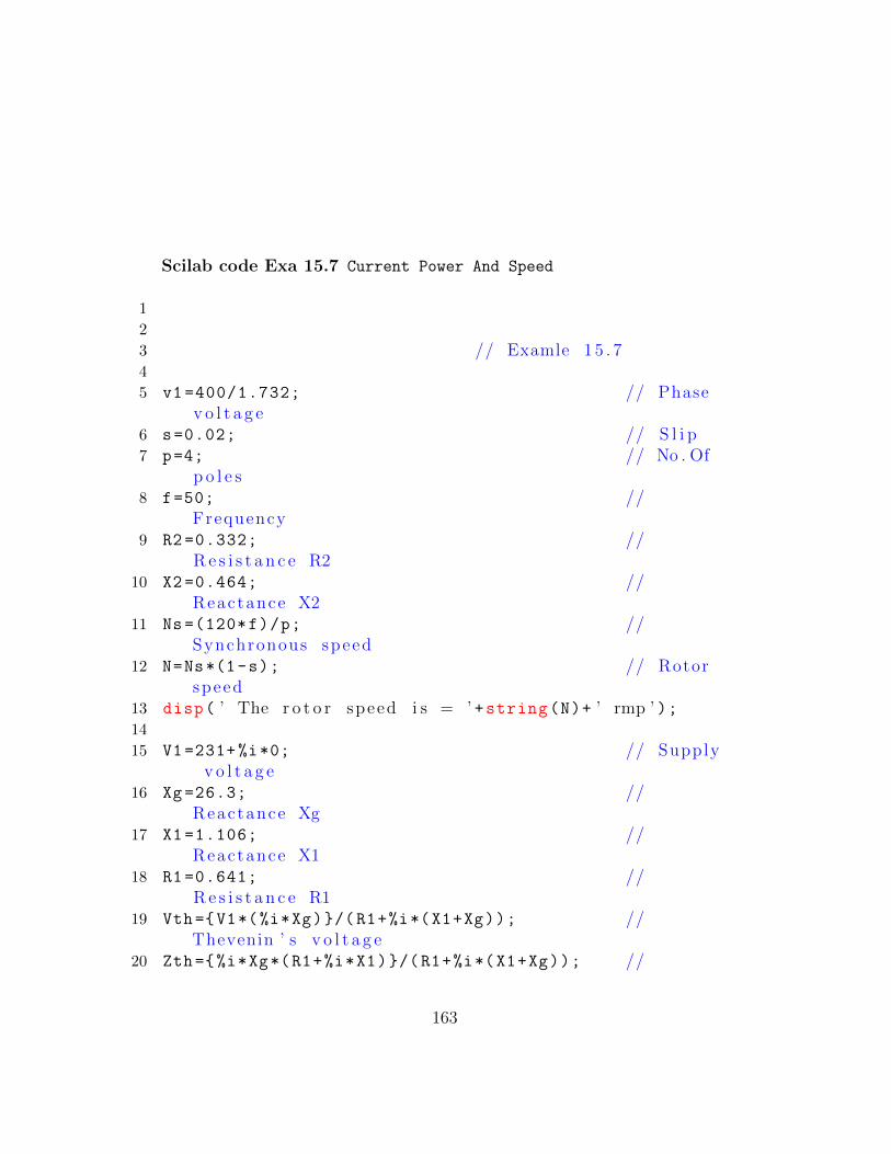
Scilab code Exa 15.7 Current Power And Speed
1
2
3 // Examle 1 5 . 74
5 v1 =400/1.732; // Phasev o l t a g e
6 s=0.02; // S l i p7 p=4; // No . Of
p o l e s8 f=50; //
Frequency9 R2 =0.332; //
R e s i s t a n c e R210 X2 =0.464; //
Reactance X211 Ns =(120*f)/p; //
Synchronous speed12 N=Ns*(1-s); // Rotor
speed13 disp( ’ The r o t o r speed i s = ’ +string(N)+ ’ rmp ’ );14
15 V1=231+%i*0; // Supplyv o l t a g e
16 Xg =26.3; //Reactance Xg
17 X1 =1.106; //Reactance X1
18 R1 =0.641; //R e s i s t a n c e R1
19 Vth={V1*(%i*Xg)}/(R1+%i*(X1+Xg)); //Thevenin ’ s v o l t a g e
20 Zth={%i*Xg*(R1+%i*X1)}/(R1+%i*(X1+Xg)); //
163
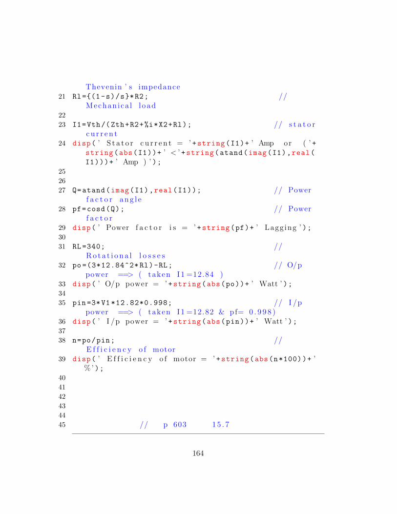
Thevenin ’ s impedance21 Rl={(1-s)/s}*R2; //
Mechan ica l l o ad22
23 I1=Vth/(Zth+R2+%i*X2+Rl); // s t a t o rc u r r e n t
24 disp( ’ S t a t o r c u r r e n t = ’ +string(I1)+ ’ Amp or ( ’ +string(abs(I1))+ ’ < ’ +string(atand(imag(I1),real(I1)))+ ’ Amp ) ’ );
25
26
27 Q=atand(imag(I1),real(I1)); // Powerf a c t o r a n g l e
28 pf=cosd(Q); // Powerf a c t o r
29 disp( ’ Power f a c t o r i s = ’ +string(pf)+ ’ Lagg ing ’ );30
31 RL=340; //R o t a t i o n a l l o s s e s
32 po =(3*12.84^2* Rl)-RL; // O/ppower ==> ( taken I1 =12.84 )
33 disp( ’ O/p power = ’ +string(abs(po))+ ’ Watt ’ );34
35 pin =3*V1 *12.82*0.998; // I /ppower ==> ( taken I1 =12.82 & pf= 0 . 9 9 8 )
36 disp( ’ I /p power = ’ +string(abs(pin))+ ’ Watt ’ );37
38 n=po/pin; //E f f i c i e n c y o f motor
39 disp( ’ E f f i c i e n c y o f motor = ’ +string(abs(n*100))+ ’% ’ );
40
41
42
43
44
45 // p 603 1 5 . 7
164
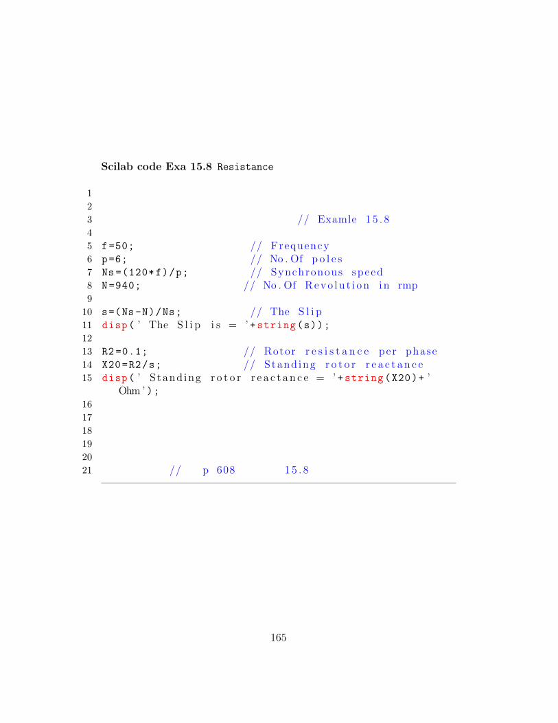
Scilab code Exa 15.8 Resistance
1
2
3 // Examle 1 5 . 84
5 f=50; // Frequency6 p=6; // No . Of p o l e s7 Ns =(120*f)/p; // Synchronous speed8 N=940; // No . Of R e v o l u t i o n i n rmp9
10 s=(Ns -N)/Ns; // The S l i p11 disp( ’ The S l i p i s = ’ +string(s));12
13 R2=0.1; // Rotor r e s i s t a n c e per phase14 X20=R2/s; // Stand ing r o t o r r e a c t a n c e15 disp( ’ S tand ing r o t o r r e a c t a n c e = ’ +string(X20)+ ’
Ohm ’ );16
17
18
19
20
21 // p 608 1 5 . 8
165

Chapter 16
DC Machines
Scilab code Exa 16.1 Voltage Current And Power
1
2 // Example 1 6 . 13
4 // ==> When Lap−wound .5
6 disp( ’ ∗ With the Armature Lap−wound , & P a r a l l e lpahts A=8 ’ );
7 Z=480; // No . Of conduc to r8 A=8; // No . Of p o l e s9 e=2.1; // Average emf i n each conduc to r
10 E=e*(Z/A); // Terminal v o l t a g e on No load11 disp( ’ Terminal v o l t a g e on No load = ’ +string(E)+ ’
Vo l t ’ );12 If=200; // Fu l l−l o ad c u r r e n t per conduc to r13 Il=If*A; // O/p c u r r e n t on f u l l −l o ad14 disp( ’ O/p c u r r e n t on f u l l −l o ad = ’ +string(Il)+ ’
Amp ’ );15 Po=Il*E; // Tota l power on f u l l −l o ad16 disp( ’ Tota l power g e n e r a t e d on f u l l −l o ad = ’ +
string(Po /1000)+ ’ kW’ );17
166
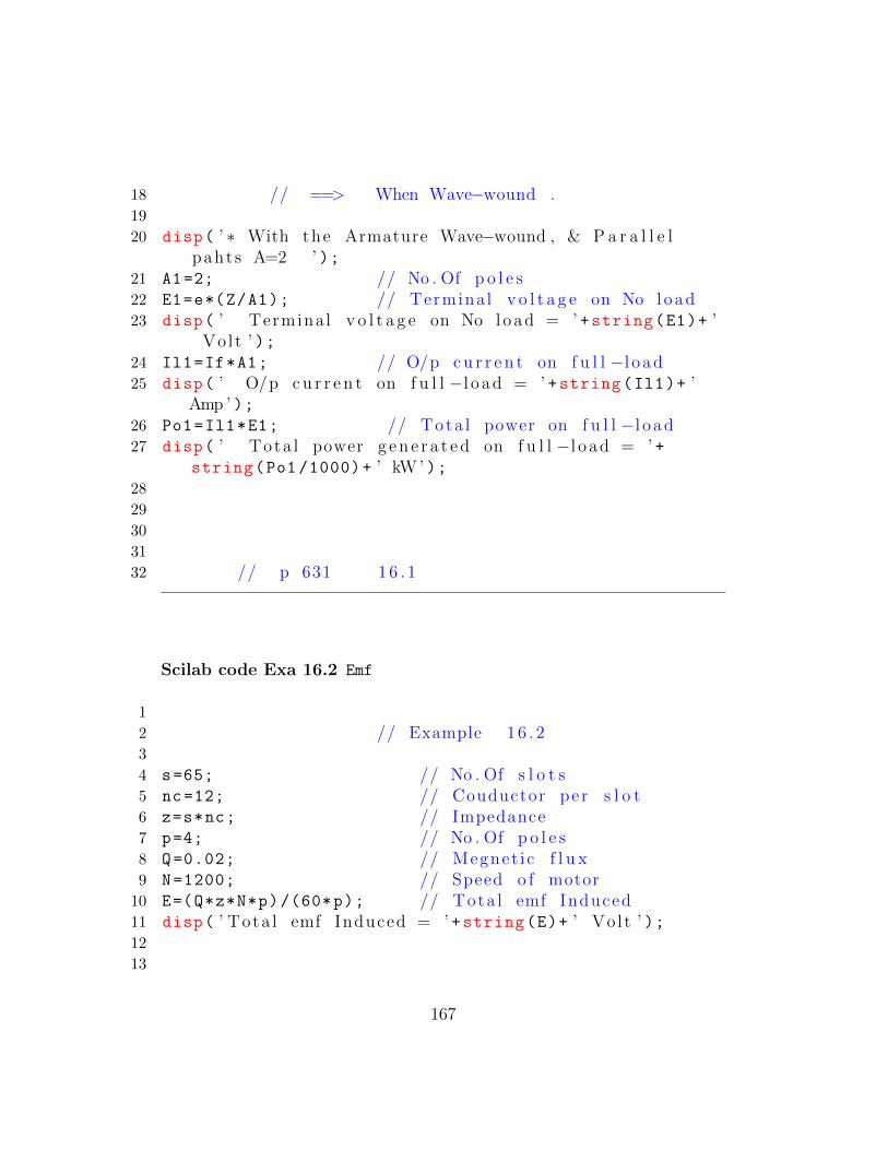
18 // ==> When Wave−wound .19
20 disp( ’ ∗ With the Armature Wave−wound , & P a r a l l e lpahts A=2 ’ );
21 A1=2; // No . Of p o l e s22 E1=e*(Z/A1); // Terminal v o l t a g e on No load23 disp( ’ Terminal v o l t a g e on No load = ’ +string(E1)+ ’
Vo l t ’ );24 Il1=If*A1; // O/p c u r r e n t on f u l l −l o ad25 disp( ’ O/p c u r r e n t on f u l l −l o ad = ’ +string(Il1)+ ’
Amp ’ );26 Po1=Il1*E1; // Tota l power on f u l l −l o ad27 disp( ’ Tota l power g e n e r a t e d on f u l l −l o ad = ’ +
string(Po1 /1000)+ ’ kW’ );28
29
30
31
32 // p 631 1 6 . 1
Scilab code Exa 16.2 Emf
1
2 // Example 1 6 . 23
4 s=65; // No . Of s l o t s5 nc=12; // Couductor per s l o t6 z=s*nc; // Impedance7 p=4; // No . Of p o l e s8 Q=0.02; // Megnet ic f l u x9 N=1200; // Speed o f motor
10 E=(Q*z*N*p)/(60*p); // Tota l emf Induced11 disp( ’ Tota l emf Induced = ’ +string(E)+ ’ Vo l t ’ );12
13
167

14
15 // p 633 1 6 . 2
Scilab code Exa 16.3 Emf
1
2 // Examle 1 6 . 33
4
5 E1=180; // Induced emf6 N1=500; // Speed o f mechine N1=5007 N2=600; // Speed o f mechine N1=6008 E2=(N2/N1)*E1; // Emf When Machine runs at
(600 rpm )9 disp( ’Emf When Machine runs at (600 rpm )= ’ +string(
E2)+ ’ Vo l t ’ );10
11
12
13 // 633 1 6 . 3
Scilab code Exa 16.4 Speed And increase in flux
1
2 // Examle 1 6 . 43
4 E1=220; // Induced emf at N=750 rpm5 E2=250; // Induced emf ( i . e E=250)6 N1=750; // Speed o f mechine at E1
=2207 N2=(E2/E1)*N1; // Speed at Constant emf E2
=250
168
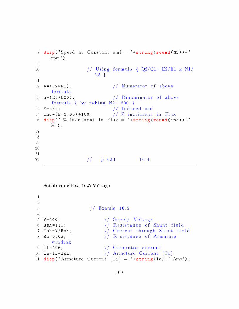
8 disp( ’ Speed at Constant emf = ’ +string(round(N2))+ ’rpm ’ );
9
10 // Using fo rmu la { Q2/Q1= E2/E1 x N1/N2 }
11
12 e=(E2*N1); // Numerator o f abovefo rmu la
13 n=(E1 *600); // Dinominator o f abovefo rmu la { by t a k i n g N2= 600 }
14 E=e/n; // Induced emf15 inc=(E -1.00) *100; // % i n c r i m e n t i n Flux16 disp( ’ % i n c r i m e n t i n Flux = ’ +string(round(inc))+ ’
% ’ );17
18
19
20
21
22 // p 633 1 6 . 4
Scilab code Exa 16.5 Voltage
1
2
3 // Examle 1 6 . 54
5 V=440; // Supply Vo l tage6 Rsh =110; // R e s i s t a n c e o f Shunt f i e l d7 Ish=V/Rsh; // Current through Shunt f i e l d8 Ra =0.02; // R e s i s t a n c e o f Armature
wind ing9 Il=496; // Generator c u r r e n t10 Ia=Il+Ish; // Armeture Current ( I a )11 disp( ’ Armeture Current ( Ia ) = ’ +string(Ia)+ ’ Amp ’ );
169
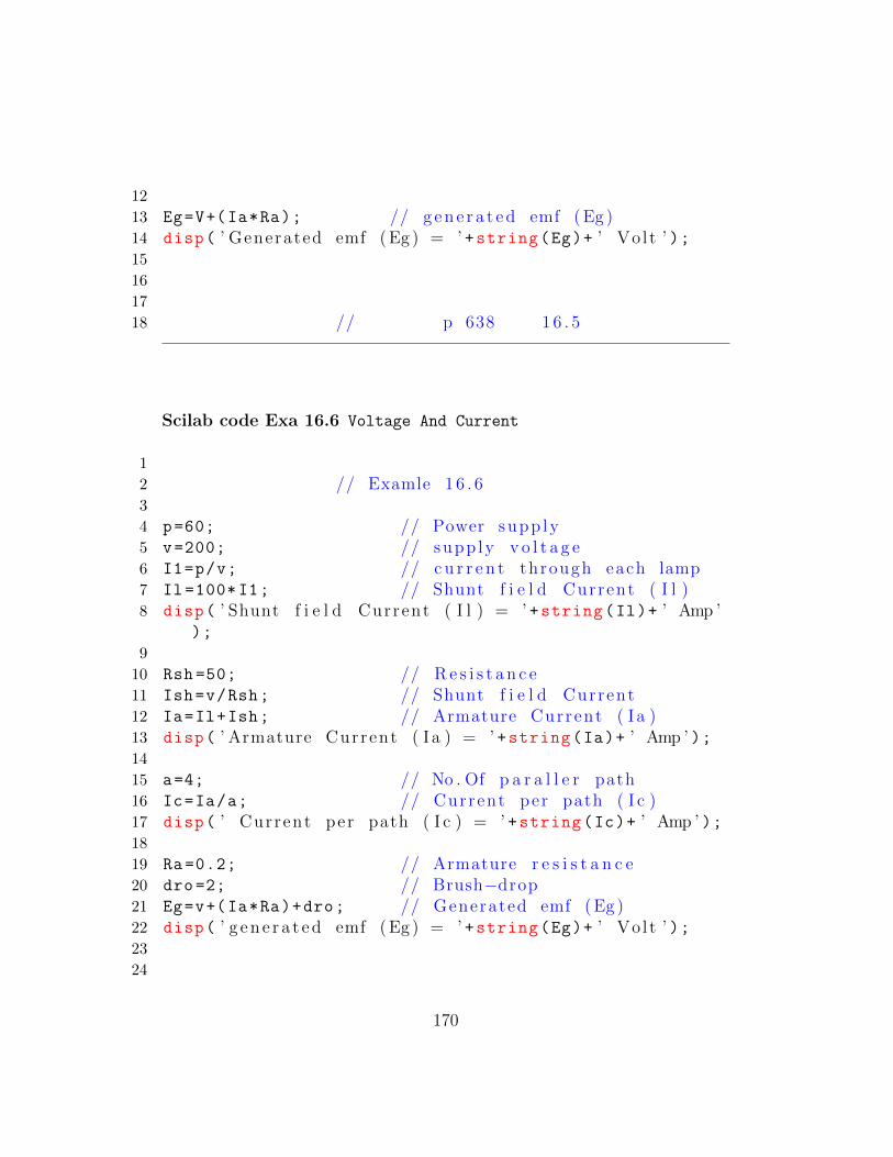
12
13 Eg=V+(Ia*Ra); // g e n e r a t e d emf ( Eg )14 disp( ’ Generated emf ( Eg ) = ’ +string(Eg)+ ’ Vo l t ’ );15
16
17
18 // p 638 1 6 . 5
Scilab code Exa 16.6 Voltage And Current
1
2 // Examle 1 6 . 63
4 p=60; // Power supp ly5 v=200; // supp ly v o l t a g e6 I1=p/v; // c u r r e n t through each lamp7 Il=100*I1; // Shunt f i e l d Current ( I l )8 disp( ’ Shunt f i e l d Current ( I l ) = ’ +string(Il)+ ’ Amp ’
);
9
10 Rsh =50; // R e s i s t a n c e11 Ish=v/Rsh; // Shunt f i e l d Current12 Ia=Il+Ish; // Armature Current ( I a )13 disp( ’ Armature Current ( I a ) = ’ +string(Ia)+ ’ Amp ’ );14
15 a=4; // No . Of p a r a l l e r path16 Ic=Ia/a; // Current per path ( I c )17 disp( ’ Current per path ( I c ) = ’ +string(Ic)+ ’ Amp ’ );18
19 Ra=0.2; // Armature r e s i s t a n c e20 dro =2; // Brush−drop21 Eg=v+(Ia*Ra)+dro; // Generated emf ( Eg )22 disp( ’ g e n e r a t e d emf ( Eg ) = ’ +string(Eg)+ ’ Vo l t ’ );23
24
170
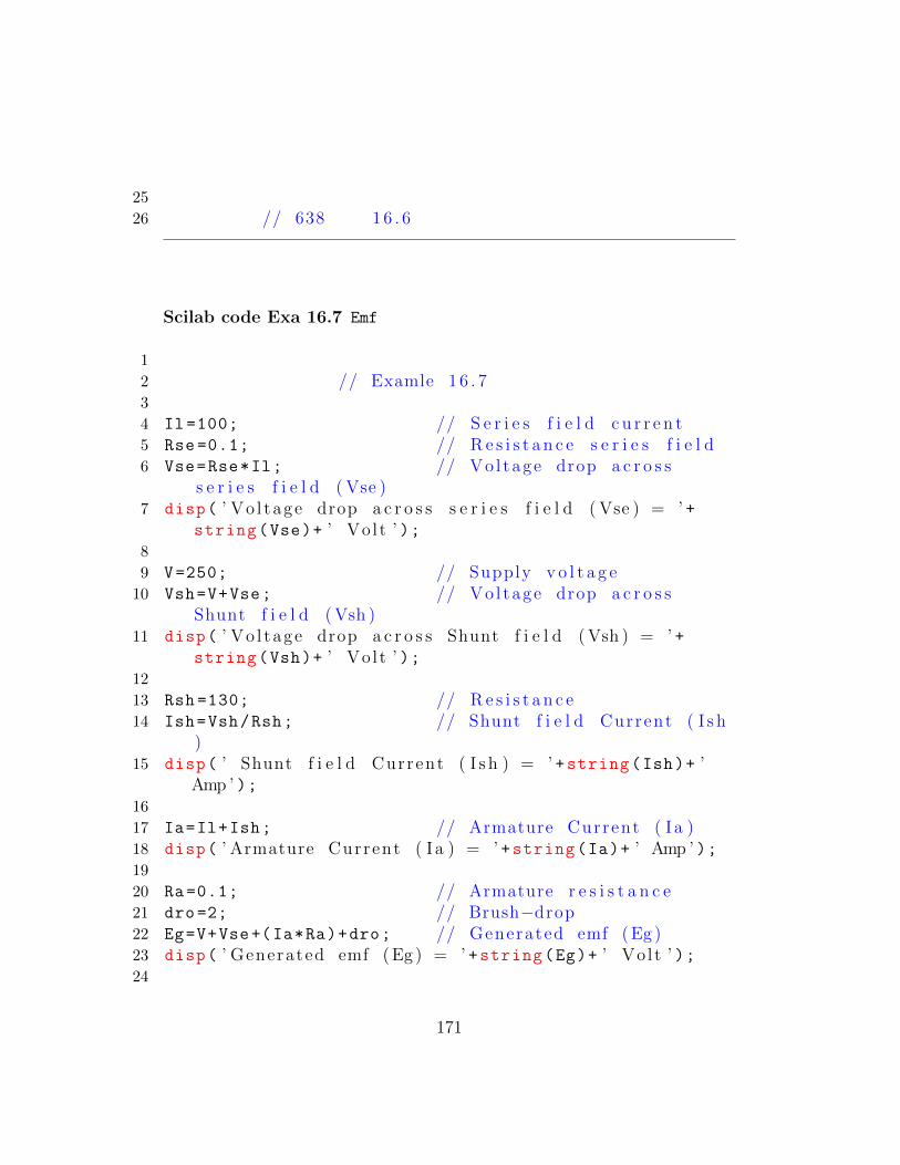
25
26 // 638 1 6 . 6
Scilab code Exa 16.7 Emf
1
2 // Examle 1 6 . 73
4 Il=100; // S e r i e s f i e l d c u r r e n t5 Rse =0.1; // R e s i s t a n c e s e r i e s f i e l d6 Vse=Rse*Il; // Vo l tage drop a c r o s s
s e r i e s f i e l d ( Vse )7 disp( ’ Vo l tage drop a c r o s s s e r i e s f i e l d ( Vse ) = ’ +
string(Vse)+ ’ Vo l t ’ );8
9 V=250; // Supply v o l t a g e10 Vsh=V+Vse; // Vo l tage drop a c r o s s
Shunt f i e l d ( Vsh )11 disp( ’ Vo l tage drop a c r o s s Shunt f i e l d ( Vsh ) = ’ +
string(Vsh)+ ’ Vo l t ’ );12
13 Rsh =130; // R e s i s t a n c e14 Ish=Vsh/Rsh; // Shunt f i e l d Current ( I s h
)15 disp( ’ Shunt f i e l d Current ( I s h ) = ’ +string(Ish)+ ’
Amp ’ );16
17 Ia=Il+Ish; // Armature Current ( I a )18 disp( ’ Armature Current ( I a ) = ’ +string(Ia)+ ’ Amp ’ );19
20 Ra=0.1; // Armature r e s i s t a n c e21 dro =2; // Brush−drop22 Eg=V+Vse+(Ia*Ra)+dro; // Generated emf ( Eg )23 disp( ’ Generated emf ( Eg ) = ’ +string(Eg)+ ’ Vo l t ’ );24
171

25
26
27 // p 638 1 6 . 7
Scilab code Exa 16.8 Voltage Efficiency And Power
1
2 // Examle 1 6 . 83
4 po =30000; // o/p power5 v=200; // Vo l tage6 Il=po/v; // Load Current ( I l )7 disp( ’ Load Current ( I l ) = ’ +string(Il)+ ’ Amp ’ );8
9 Rsh =50; // Shunt f i e l dr e s i s t a n c e R1
10 Ish=v/Rsh; // Shunt f i e l d Current11 Ia=Il+Ish; // Armature Current ( I a
)12 Ra =0.05; // Shunt f i e l d
r e s i s t a n c e R213 Eg=v+(Ia*Ra); // Generated emf ( Eg )14 disp( ’ Generated emf ( Eg ) = ’ +string(Eg)+ ’ Vo l t ’ );15
16 Cu=Ish^2* Rsh+Ia^2*Ra; // The copper L o s s e s (Cu)
17 disp( ’ The copper L o s s e s (Cu) = ’ +string(Cu)+ ’ W’ );18
19 e=po *100/(1000+ po+Cu); // The E f f i c i e n c y ( e )20 disp( ’ The E f f i c i e n c y ( e ) = ’ +string (e)+ ’ % ’ );21
22
23
24 // p 641 1 6 . 8
172
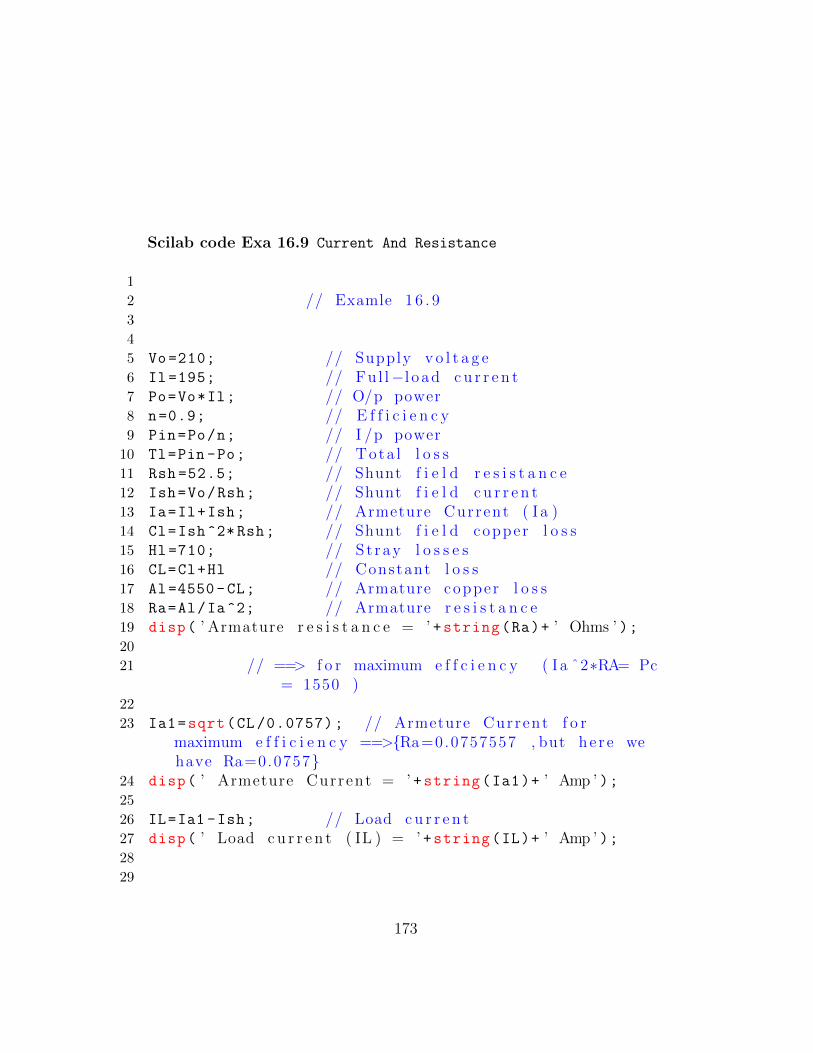
Scilab code Exa 16.9 Current And Resistance
1
2 // Examle 1 6 . 93
4
5 Vo=210; // Supply v o l t a g e6 Il=195; // Fu l l−l o ad c u r r e n t7 Po=Vo*Il; // O/p power8 n=0.9; // E f f i c i e n c y9 Pin=Po/n; // I /p power10 Tl=Pin -Po; // Tota l l o s s11 Rsh =52.5; // Shunt f i e l d r e s i s t a n c e12 Ish=Vo/Rsh; // Shunt f i e l d c u r r e n t13 Ia=Il+Ish; // Armeture Current ( I a )14 Cl=Ish^2* Rsh; // Shunt f i e l d copper l o s s15 Hl=710; // St ray l o s s e s16 CL=Cl+Hl // Constant l o s s17 Al=4550-CL; // Armature copper l o s s18 Ra=Al/Ia^2; // Armature r e s i s t a n c e19 disp( ’ Armature r e s i s t a n c e = ’ +string(Ra)+ ’ Ohms ’ );20
21 // ==> f o r maximum e f f c i e n c y ( Ia ˆ2∗RA= Pc= 1550 )
22
23 Ia1=sqrt(CL /0.0757); // Armeture Current f o rmaximum e f f i c i e n c y ==>{Ra=0.0757557 , but he r e wehave Ra=0.0757}
24 disp( ’ Armeture Current = ’ +string(Ia1)+ ’ Amp ’ );25
26 IL=Ia1 -Ish; // Load c u r r e n t27 disp( ’ Load c u r r e n t ( IL ) = ’ +string(IL)+ ’ Amp ’ );28
29
173
30
31 // p 642 1 6 . 9
Scilab code Exa 16.10 Turns
1
2 // Examle 1 6 . 1 03
4 i1=4; // No load c u r r e n t5 i2=6; // Fu l l−l o ad c u r r e n t6 n=1500; // No . Of t u r n s per p o l e s7 At1=i1*n; // Amper Turns per p o l e on
No Load8 disp( ’ Amper Turns per p o l e on No Load = ’ +string(
At1)+ ’ At ’ );9
10 At2=i2*n; // Amper Turns per p o l e onF u l l Load
11 disp( ’ Amper Turns per p o l e on F u l l Load = ’ +string(At2)+ ’ At ’ );
12
13 At=At2 -At1; // Amper Turns per p o l e o fs e i r e s wind ing
14 disp( ’ Amper Turns per p o l e o f s e i r e s wind ing = ’ +string(At)+ ’ At ’ );
15
16 Nse=At/100; // F u l l Load Current17 disp( ’ F u l l Load Current = ’ +string(Nse));18
19
20
21
22
23 // p 647 1 6 . 1 0
174
Scilab code Exa 16.11 Voltage
1
2
3 // Examle 1 6 . 1 14
5 V=250; // Supply v o l t a g e6 Rsh =250; // F i e l d wind ing r e s i s t a n c e7 Ish=V/Rsh; // The shunt f i e l d c u r r e n t (
I s h )8 disp( ’ The Shunt f i e l d c u r r e n t ( I s h ) = ’ +string(Ish)
+ ’ Amp ’ );9 Il=41; // Fu l l−l o ad c u r r e n t10 Ia=Il-Ish; // Armature c u r r e n t11 disp( ’ The Armature c u r r e n t c u r r e n t ( Ia ) = ’ +string(
Ia)+ ’ Amp ’ );12 Ra=0.1; // Armature r e s i s t a n c e13 Eb=V-(Ia*Ra); // back emf14 disp( ’ The back emf (Eb) = ’ +string(Eb)+ ’ Vo l t ’ );15
16
17
18
19 // p 649 1 6 . 1 1
Scilab code Exa 16.12 Speed
1
2
3 // Examle 1 6 . 1 24
5 V=440; // Supply v o l t a g e
175

6 Ia=50; // Armature c u r r e r n t7 Ra =0.28; // Armature r e s i s t a n c e8 a=2; // No . Of p a r a l l e r path9 Q=0.023; // Megnet ic f l u x per p o l e
10 z=888; // Impedence11 p=4; // No . Of p o l e s12 Eb=V-(Ia*Ra); // Back emf (Eb)13 disp( ’ Back emf (Eb) = ’ +string(Eb)+ ’ Vo l t ’ );14
15 N=(60*a*Eb)/(Q*z*p); // Speed o f the moter16 disp( ’ Speed o f the moter = ’ +string(round(N))+ ’ rms
’ );17
18
19
20
21 // p 649 1 6 . 1 2
Scilab code Exa 16.13 Speed
1
2 // Examle 1 6 . 1 33
4 At=900; // Speed o f motor5 V=460; // Supply v o l t a g e6 kQ=V/At; // O r i g n a l Flux7 disp( ’ O r i g n a l Flux = ’ +string(kQ));8
9 V1=200; // Chenged Supply v o l t a g e10 N=V1 /(0.7* kQ); // Speed o f Motor When
Supply (200 V)11 disp( ’ Speed o f Motor When Supply (200 V) = ’ +string
(round(N))+ ’ rpm ’ );12
13
176

14
15
16
17 // p 649 1 6 . 1 3
Scilab code Exa 16.14 Speed And Torque
1
2 // Examle 1 6 . 1 43
4 V=480;
5 Ia=110; // Armature c u r r e r n t6 Ra=0.2; // Armature r e s i s t a n c e7 a=6; // No . Of p a r a l l e r path8 p=6; // No . Of p o l e s9 Q=0.05; // Megnet ic f l u x per p o l e
10 z=864; // Impedence11 Eb=V-(Ia*Ra); // Generated emf (Eb)12 disp( ’ Generated emf (Eb) = ’ +string(Eb)+ ’ Vo l t ’ );13
14 N=(60*a*Eb)/(Q*z*p); // Speed o f the moter15 disp( ’ Speed o f the moter = ’ +string(round(N))+ ’ rms
’ );16
17 // ==> Using Formula { td= Qz/2TT x ( p/A)xIa }
18
19 x=(Q*z)/(2* %pi); // f o r s i m l i c i t y20 td=(p/a)*Ia*(x); // Tota l Torque (Td)21 disp( ’ Tota l Torque (Td) = ’ +string (round(td))+ ’ Nm
’ );22
23
24
25
177
26
27 // p 650 1 6 . 1 4
Scilab code Exa 16.15 Power
1
2
3 // Examle 1 6 . 1 54
5 t=2000; // Torque6 N=900; // Speed7 Ploss =8000; // Power l o s s8 Pin =(2* %pi*t*N)/60; // Input Power ( Pin )9 disp( ’ Input Power ( Pin ) ’ +string(Pin /1000)+ ’ kW’ );
10
11 Pd=Pin -Ploss; // Power Generated i nArmature (Pd)
12 disp( ’ Power Generated i n Armature (Pd) = ’ +string(Pd /1000)+ ’ kW’ );
13
14
15
16 // p 651 1 6 . 1 5
Scilab code Exa 16.16 Speed
1
2 // Example 1 6 . 1 63
4 V=230; // Supply v o l t a g e5 Ia=110; // Current6 Ra =0.12; // R e s i s t a n c e7 Rse =0.03; // S e r i e s f i e l d r e s i s t a n c e
178
8 E1=V-Ia*(Ra+Rse); // Emf Generated9
10 // But f o r the Given machine ( E1= QZNP/60A= kQ1N1 )
11
12 N1=600; // No . Of t u r n s13 Q1 =0.024; // Megnet ic f l u x14 k=E1/(Q1*N1); // Constant15
16 Ia1 =50; // Current o f 50A17 E2=V-[Ia1*(Ra+Rse)]; // Emf Generated18
19 // We know tha t E2=k∗Q2∗N220
21 Q2 =0.016; // Megnet ic f l u x22 N2=E2/(k*Q2); // New speed23 disp( ’ The new speed i s = ’ +string(round(N2))+ ’ rpm ’
);
24
25
26
27
28 // p 653 1 6 . 1 6
Scilab code Exa 16.17 Current
1
2 // Example 1 6 . 1 73
4 Ra=0.2; // R e s i s t a n c e5 V=250; // Supply v o l t a g e6 Eb=0; // Vo l tage at r e s t7 Ia=(V-Eb)/Ra; // Current drawn by the
machine at Eb=2008 disp( ’ Current drawn by the machine at (Eb=0) = ’ +
179
string(Ia)+ ’ Amp ’ );9
10 Eb1 =200; // Vo l tage at Eb=20011 Ia1=(V-Eb1)/Ra; // Current drawn by the
machine at Eb=20012 disp( ’ Current drawn by the machine at (Eb=200) = ’ +
string(Ia1)+ ’ Amp ’ );13
14 Eb2 =250; // Vo l tage at Eb=25015 Ia2=(V-Eb2)/Ra; // Current drawn by the
machine at Eb=25016 disp( ’ Current drawn by the machine at (Eb=250) = ’ +
string(Ia2)+ ’ Amp ’ );17
18 Eb3 =-250; // Vo l tage at Eb=−25019 Ia3=(V-Eb3)/Ra; // Current drawn by the
machine at Eb=−25020 disp( ’ Current drawn by the machine at (Eb=−250) = ’
+string(Ia3)+ ’ Amp ’ );21
22
23
24
25
26 // p 653 1 6 . 1 7
Scilab code Exa 16.18 Speed And Torque
1
2 // Examle 1 6 . 1 83
4 V=480; // Supply v o l t a g e5 Ia=110; // Armature c u r r e r n t6 Ra =0.18; // S e r i e s f i e l d
r e s i s t a n c e R1
180
7 Rse =0.02; // S e r i e s f i e l dr e s i s t a n c e R2
8 Eb=V-Ia*(Ra+Rse); // Generated emf9 disp( ’ Generated emf = ’ +string(Eb)+ ’ Vo l tage ’ );10
11 a=6; // No . Of p a r a l l e r path12 Q=0.05; // Megnet ic f l u x13 z=864; // Conductor14 p=6; // No . Of p o l e s15 N=(60*a*Eb)/(Q*z*p); // Speed o f a Motor16 disp( ’ Speed o f a Motor = ’ +string(round(N))+ ’ rpm ’ )
;
17
18 Td=(60*Eb*Ia)/(2* %pi*N); // The Torque Develop byArmeture
19 disp( ’ The Torque Develop by Armeture = ’ +string(round(Td))+ ’ Nm’ );
20
21
22
23 // p 654 1 6 . 1 8
Scilab code Exa 16.19 Resistance
1
2
3 // Examle 1 6 . 1 94
5 V=220; // Supply v o l t a g e6 Ia=22; // Armature c u r r e r n t7 Ra =0.45; // Armature r e s i s t a n c e8 E1=V-(Ia*Ra); // Generated emf9 disp( ’ Generated emf = ’ +string(E1)+ ’ Vo l tage ’ );10
11 N1=700; // Speed o f motor i n Shunt
181

12 N2=450; // Speed o f motor i n S e r i e s13 E2=(N2*E1)/N1; // Emf o f Shunt motor14 disp( ’ Emf o f Shunt motor = ’ +string(E2)+ ’ v o l t a g e ’ )
;
15
16 Va=Ia*Ra; // Armature v o l t a g e17 R=(V-(E2+Va))/Ia; // R e s i s t a n c e with Armature18 disp( ’ R e s i s t a n c e with Armature = ’ +string(R)+ ’ ohms
’ );19
20
21
22 // p 654 1 6 . 1 9
Scilab code Exa 16.20 Speed
1
2
3 // Examle 1 6 . 2 04
5 V=230; // Supp l t v o l t a g e6 Ia1 =40; // Armature c u r r e r n t Ia17 Ra=0.2; // Armature r e s i s t a n c e8 Rse =0.1; // S e r i e s f i e l d r e s i s t a n c e9 E1=V-Ia1*(Ra+Rse); // Back emfat (24 A)
10 disp( ’ Back emfat (24 A) = ’ +string(E1)+ ’ Vo l tage ’ );11
12 Ia2 =20; // Armature c u r r e r n t Ia213 E2=V-Ia2*(Ra+Rse); // Back emfat (20 A)14 disp( ’ Back emfat (20 A) = ’ +string(E2)+ ’ Vo l tage ’ );15
16 N1 =1000; // Speed o f a Motor at I=40A
17 N2=(E2*N1)/(E1 *0.6); // Speed o f a Motor18 disp( ’ Speed o f a Motor = ’ +string(round(N2))+ ’ rpm ’
182

);
19
20
21
22
23 // p 654 1 6 . 2 0
183
Chapter 17
Fractional Horse Power Motors
Scilab code Exa 17.1 Slip And Efficiency
1
2 // Examle 1 7 . 13
4 f=50; // Frequency5 p=4; // No . Of p o l e s6 Ns =(120*f)/p; // Synchronous speed7 N=1410; // No . Of R e v o l u t i o n i n rmp8 I=2.9; // I /p c u r r e n t9 V=230; // Supply v o l t a g e
10 CosQ =0.71; // Power f a c t o r11 s=(Ns -N)/Ns; // The S l i p12 disp( ’ The S l i p i s = ’ +string(s*100)+ ’ % ’ );13
14 po=375; // O/p power15 pin=V*I*CosQ; // I /p power16 eff=po/pin; // E f f i c i e n c y17 disp( ’ The e f f i c i e n c y i s = ’ +string(eff *100)+ ’ % ’ );18
19
20
21
184
22
23
24 // p 683 1 7 . 1
Scilab code Exa 17.2 Current Phase Angle And Power Factor
1
2 // Examle 1 7 . 23
4
5 zm=(5+%i*12); // Impedence o f main−Winding
6 za=(12+%i*5); // Impedence o f s t a r t i n g −Winding
7 V=230+ %i*0; // Supply v o l t a g e8 Im=V/zm; // Current i n main−Winding9 disp( ’ The Current i n main−Winding = ’ +string(Im)+ ’
Amp or ( ’ +string(abs(Im))+ ’ < ’ +string(atand(imag(Im),real(Im)))+ ’ Amp ) ’ );
10
11 Ia=V/za; // Current i n s t a r t i n g −Winding
12 disp( ’ The Current i n s t a r t i n g −Winding = ’ +string(Ia)+ ’ Amp or ( ’ +string(abs(Ia))+ ’ < ’ +string(atand(imag(Ia),real(Ia)))+ ’ Amp ) ’ );
13
14 Il=Im+Ia; // The l i n e Current15 disp( ’ The l i n e Current = ’ +string(Il)+ ’ Amp or ( ’
+string(abs(Il))+ ’ < ’ +string(atand(imag(Il),real(Il)))+ ’ Amp ) ’ );
16
17 Qa= -22.62; // Phase a n g l e o f s t a r t i n g −winding
18 Qm= -67.38; // Phase a n g l e o f main−winding
185

19 Q=Qa -Qm; // The phase d i s p l a c e m e n t (Q)
20 disp( ’ The phase d i s p l a c e m e n t (Q) = ’ +string(Q)+ ’ i. e = ’ +string(round(Q))+ ’ D i g r e e ’ );
21
22 pf=cosd(round(Q)); // The Power f a c t o r23 disp( ’ The Power f a c t o r i s = ’ +string(pf)+ ’ l a g g i n g ’
);
24
25
26
27 // p 683 1 7 . 2
Scilab code Exa 17.3 Capacitor
1
2 // Examle 1 7 . 33
4 Xm=20; // I n d u c t i v e r e a c t a n c e o fMain−winding
5 Rm=2; // Main−winding r e s i s t a n c e6 Ra=25; // A u x i l l i a r y −winding
r e s i s t a n c e7 f=50; // Frequency8 Xa=5; // I n d u c t i v e r e a c t a n c e o f
A u x i l l i a r y −winding9 Qm=atand(Xm/Rm); // Angle o f Main−winding10 Qa=Qm -90; // Angle o f A u x i l l i a r y −
winding11 Xc=Xa -(tand(Qa)*Ra); // C a p a c i t i v e r e a c t a n c e12 C=1/(2* %pi*f*7.495); // C a p a c i t o r (C) ==> { Xc
= 7 . 5 , but t a k i n g Xc= 7 . 4 9 5 }13 disp( ’ The v a l u e o f C a pa c i t o r (C) = ’ +string(C)+ ’ F ’ )
;
14
186
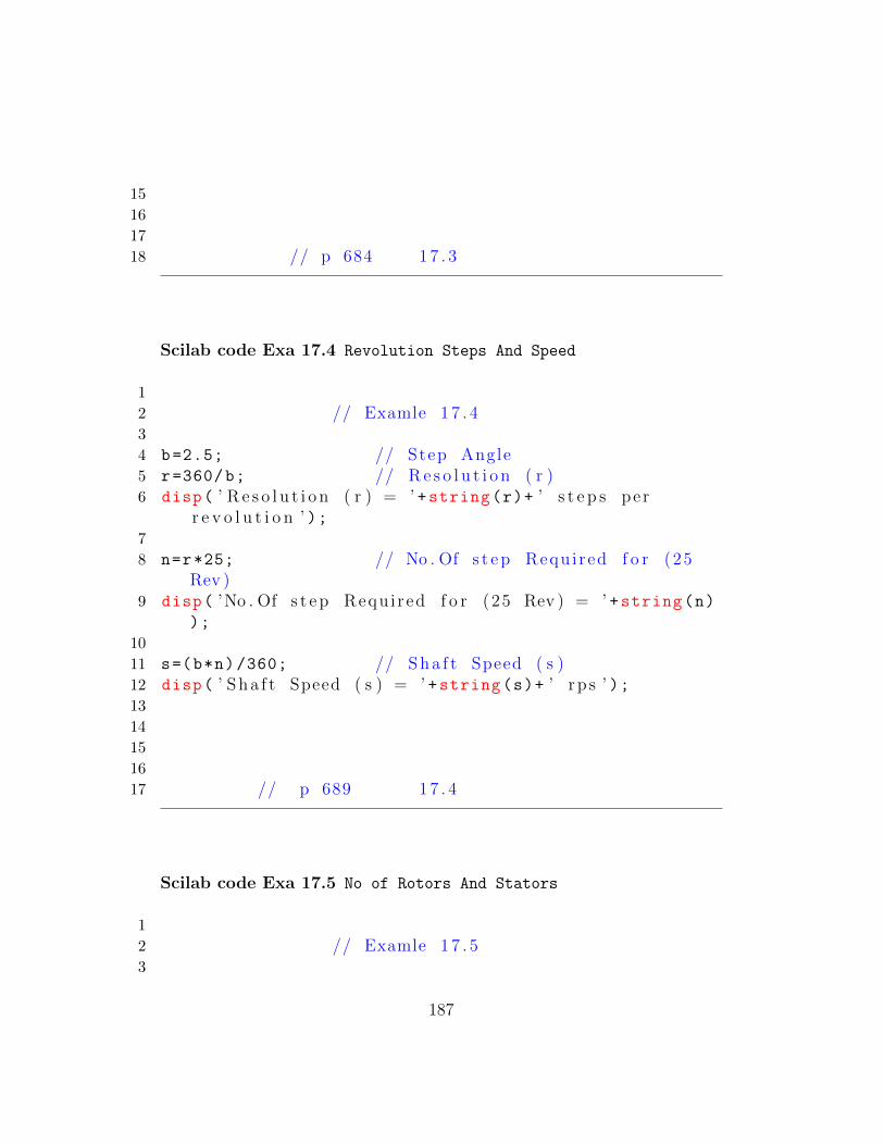
15
16
17
18 // p 684 1 7 . 3
Scilab code Exa 17.4 Revolution Steps And Speed
1
2 // Examle 1 7 . 43
4 b=2.5; // Step Angle5 r=360/b; // R e s o l u t i o n ( r )6 disp( ’ R e s o l u t i o n ( r ) = ’ +string(r)+ ’ s t e p s per
r e v o l u t i o n ’ );7
8 n=r*25; // No . Of s t e p Requ i red f o r (25Rev )
9 disp( ’No . Of s t e p Requ i red f o r (25 Rev ) = ’ +string(n));
10
11 s=(b*n)/360; // S h a f t Speed ( s )12 disp( ’ S h a f t Speed ( s ) = ’ +string(s)+ ’ r p s ’ );13
14
15
16
17 // p 689 1 7 . 4
Scilab code Exa 17.5 No of Rotors And Stators
1
2 // Examle 1 7 . 53
187
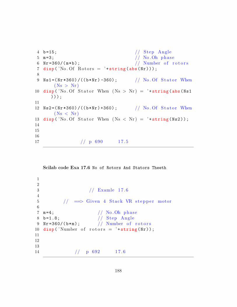
4 b=15; // Step Angle5 m=3; // No . Oh phase6 Nr =360/(m*b); // Number o f r o t o r s7 disp( ’No . Of Rotor s = ’ +string(abs(Nr)));8
9 Ns1=(Nr*360) /((b*Nr) -360); // No . Of S t a t o r When( Ns > Nr )
10 disp( ’No . Of S t a t o r When ( Ns > Nr ) = ’ +string(abs(Ns1)));
11
12 Ns2=(Nr*360) /((b*Nr)+360); // No . Of S t a t o r When( Ns < Nr )
13 disp( ’No . Of S t a t o r When ( Ns < Nr ) = ’ +string(Ns2));14
15
16
17 // p 690 1 7 . 5
Scilab code Exa 17.6 No of Rotors And Stators Theeth
1
2
3 // Examle 1 7 . 64
5 // ==> Given 4 Stack VR s t e p p e r motor6
7 m=4; // No . Oh phase8 b=1.8; // Step Angle9 Nr =360/(b*m); // Number o f r o t o r s
10 disp( ’ Number o f r o t o r s = ’ +string(Nr));11
12
13
14 // p 692 1 7 . 6
188

Chapter 18
Electrical MeasuringInstruments
Scilab code Exa 18.1 Torque
1
2 // Examle 1 8 . 13
4 I=0.015; // Current i n a c o i l5 B=0.2; // Megnet ic f l u x d e n s i t y6 l=0.02; // Length o f megnet i c f i e l d7 n1=42; // No . Of t u r n s N18 r=0.0125; // r a d i u s o f c o i l9 n2=43; // No . Of t u r n s N2
10 F1=I*B*l*n1; // The f o r c e on(42−Conductors )
11 disp( ’ The f o r c e on(42−Conductors ) = ’ +string(F1)+ ’ N’ );
12
13 F2=I*B*l*n2; // The f o r c e on(43−Conductors )
14 disp( ’ The f o r c e on(43−Conductors ) = ’ +string(F2)+ ’ N’ );
15
189
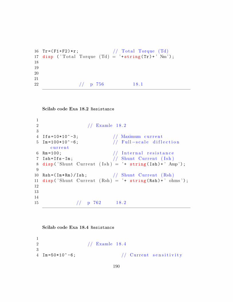
16 Tr=(F1+F2)*r; // Tota l Torque (Td)17 disp ( ’ Tota l Torque (Td) = ’ +string(Tr)+ ’ Nm’ );18
19
20
21
22 // p 756 1 8 . 1
Scilab code Exa 18.2 Resistance
1
2 // Examle 1 8 . 23
4 Ifs =10*10^ -3; // Maximum c u r r e n t5 Im =100*10^ -6; // Fu l l−s c a l e d i f l e c t i o n
c u r r e n t6 Rm=100; // I n t e r n a l r e s i s t a n c e7 Ish=Ifs -Im; // Shunt Current ( I s h )8 disp( ’ Shunt Current ( I s h ) = ’ + string(Ish)+ ’ Amp ’ );9
10 Rsh=(Im*Rm)/Ish; // Shunt Current ( Rsh )11 disp( ’ Shunt Current ( Rsh ) = ’ + string(Rsh)+ ’ ohms ’ );12
13
14
15 // p 762 1 8 . 2
Scilab code Exa 18.4 Resistance
1
2 // Examle 1 8 . 43
4 Im=50*10^ -6; // Current s e n s i t i v i t y
190

5 Rm=100; // I n t e r n a l r e s i s t a n c e6 Vf=50; // vo l t−meter range7 Rs=(Vf/Im)-Rm; // The Value o f R e s i s t e r
( Rs )8 disp ( ’ The Value o f R e s i s t e r ( Rs ) = ’ +string(Rs
/1000)+ ’ k i l o−ohms ’ );9
10
11
12
13 // p 767 1 8 . 4
Scilab code Exa 18.5 Resistance And Multiplying Factor
1
2 // Examle 1 8 . 53
4 Im=50*10^ -6; // Current s e n s i t i v i t y5 Rm =1000; // I n t e r n a l r e s i s t a n c e6 Vf=50; // vo l t−meter range7 Rs=(Vf/Im)-Rm; // The Value o f R e s i s t e r (
Rs )8 disp ( ’ The Value o f R e s i s t e r ( Rs ) = ’ +string(Rs
/1000)+ ’ k i l o−ohms ’ );9
10 n=Vf/(Im*Rm); // The Vo l tage M u l t i p l y i n gFacto r (N)
11 disp( ’ The Vo l tage M u l t i p l y i n g Facto r (N) = ’ +string(n));
12
13
14
15 // p 767 1 8 . 5
191

Scilab code Exa 18.6 Voltage And Error
1
2 // Examle 1 8 . 63
4 s=1000; // S e n s i t i v i t y o fVolt−meter A
5 r=50; // Load r e s i s t a n c e6 Vt=50; // Range o f vo l t−
meter7 Ri1=s*r; // I n t e r n a l
r e s i s t a n c e o f Volt−meter A8 V1 =150*{25000/(100000+25000) }; // Vo l tage i n I s t
Meter9 disp( ’ Vo l tage i n I s t Meter (V) = ’ +string(V1)+ ’ Vo l t
’ );10
11 s1 =20000; // S e n s i t i v i t y o fVolt−meter B
12 Ri2=s1*r; // I n t e r n a lr e s i s t a n c e o f Volt−meter B
13 V2 =150*{47600/(100000+47600) }; // Vo l tage i n 2ndMeter
14 disp( ’ Vo l tage i n 2nd Meter (V) = ’ +string(V2)+ ’ Vo l t’ );
15
16 Er1=(Vt -V1)*100/Vt; // % Erro r i n I s tmeter
17 disp( ’% Er ro r i n I s t meter = ’ +string(Er1)+ ’ % ’ );18
19 Er2=(Vt -48.36) *100/ Vt; // % Erro r i n 2ndmeter ==> { V2=48.3739 , but t a k i n g V2= 4 8 . 3 6 }
20 disp( ’% Er ro r i n 2nd meter = ’ +string(Er2)+ ’ % ’ );21
192

22
23
24
25 // p 770 1 8 . 6
Scilab code Exa 18.7 Angle of Deflection
1
2 // Examle 1 8 . 73
4 k=60/20; // Der ived from { Q= k x I}
5 i=12; // Current6 Q1=k*i; // D i f l e c t i o n f o r Spr ing−
Cont ro l Current7 disp( ’ D i f l e c t i o n f o r Spr ing−Cont ro l Current = ’ +
string(Q1)+ ’ D i g r e e ’ );8
9 k1=sind (60) /20; // Der ived from { SinQ= k xI }
10 Q2=asind(k1*12); // D i f l e c t i o n f o r Gravity−Cont ro l Current
11 disp( ’ D i f l e c t i o n f o r Gravity−Cont ro l Current = ’ +string(Q2)+ ’ D i g r e e ’ );
12
13
14
15 // 775 1 8 . 7
Scilab code Exa 18.8 Deflection in the Torque
1
2
193
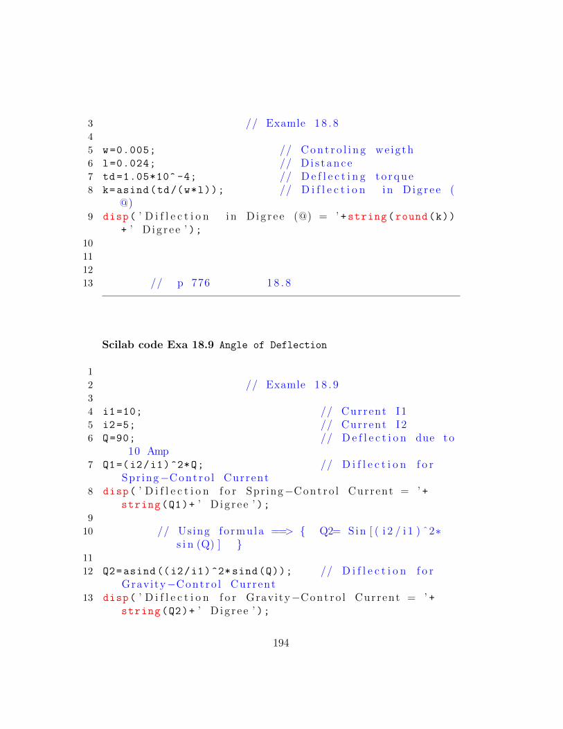
3 // Examle 1 8 . 84
5 w=0.005; // C o n t r o l i n g we ig th6 l=0.024; // D i s t a n c e7 td =1.05*10^ -4; // D e f l e c t i n g t o r q u e8 k=asind(td/(w*l)); // D i f l e c t i o n i n D ig r e e (
@)9 disp( ’ D i f l e c t i o n i n D ig r e e (@) = ’ +string(round(k))
+ ’ D i g r e e ’ );10
11
12
13 // p 776 1 8 . 8
Scilab code Exa 18.9 Angle of Deflection
1
2 // Examle 1 8 . 93
4 i1=10; // Current I15 i2=5; // Current I26 Q=90; // D e f l e c t i o n due to
10 Amp7 Q1=(i2/i1)^2*Q; // D i f l e c t i o n f o r
Spr ing−Cont ro l Current8 disp( ’ D i f l e c t i o n f o r Spr ing−Cont ro l Current = ’ +
string(Q1)+ ’ D i g r e e ’ );9
10 // Using fo rmu la ==> { Q2= Sin [ ( i 2 / i 1 ) ˆ2∗s i n (Q) ] }
11
12 Q2=asind((i2/i1)^2* sind(Q)); // D i f l e c t i o n f o rGravity−Cont ro l Current
13 disp( ’ D i f l e c t i o n f o r Gravity−Cont ro l Current = ’ +string(Q2)+ ’ D i g r e e ’ );
194
Scilab code Exa 18.10 Current
1
2
3 // Examle 1 8 . 1 04
5 w=0.004; // width o f the c o i l6 l=0.005; // Length o f the c o i l7 A=w*l; // Area o f the c o i l8 B=0.1; // Megnet ic f l u x d e n s i t y9 n=80; // No . Of t u r n s
10 tc =0.5*60*10^ -6; // C o n t r o l i n g t o r q u e11 td=3*10^ -3; // D e f l e c t i n g t o r q u e12 I=tc/(B*n*A); // Current13 disp( ’ Current ( I ) = ’ +string(I)+ ’ Amp ’ );14
15
16
17 // p 777 1 8 . 1 0
195
Related Documents