Scilab Manual for Image Processing by Mr Gautam Pal ...

Scilab Manual forImage Processingby Mr Gautam Pal

Computer EngineeringTripura Institute of Technlogy1

Solutions provided byMr R.Senthilkumar- Assistant Professor

Electronics EngineeringInstitute of Road and Transport Technology

February 23, 2022

1Funded by a grant from the National Mission on Education through ICT,http://spoken-tutorial.org/NMEICT-Intro. This Scilab Manual and Scilab codeswritten in it can be downloaded from the ”Migrated Labs” section at the websitehttp://scilab.in

1

Contents

List of Scilab Solutions 4

1 Distance and Connectivity: To understand the notion ofconnectivity and neighborhood defined for a point in animage. 6

2 Image Arithmetic - To learn to use arithmetic operationsto combine images. 8

3 Image Arithmetic –To study the effect of these operationson the dynamic range of the output image. 11

4 Image Arithmetic –To study methods to enforce closureforces the output image to also be an 8 bit image. 15

5 Affine Transformation - To learn basic image transformationi) Translation ii) Rotation iii) Scaling 19

6 Affine Transformation –To learn the role of interpolationoperation i) Bi-linear ii) Bi-cubic iii) nearest neighbor 21

7 Affine Transformation –To learn the effect of multiple trans-formations i) Significance of order in which one carried out 23

8 Point Operations - To learn image enhancement throughpoint transformation-i)Linear transformation ii) Non-lineartransformation 25

9 Neighborhood Operations - To learn about neighborhood

2

operations and use them for i) Linear filtering ii) Non-linearfiltering 28

10 Neighborhood Operations –To study the effect of the sizeof neighborhood on the result of processing 30

11 Image Histogram - To understand how frequency distribu-tion can be used to represent an image. 32

12 Image Histogram –To study the correlation between thevisual quality of an image with its histogram. 35

13 Fourier Transform: To understand some of the fundamentalproperties of the Fourier transform. 38

14 Colour Image Processing: To learn colour images are han-dled and processed i)Models for representing colour ii) Meth-ods of proces 40

15 Morphological Operations: To understand the basics of mor-phological operations which are used in analyzing the formand shape de 43

3

List of Experiments

Solution 1.1 Exp1 . . . . . . . . . . . . . . . . . . . . . . . . . 6Solution 2.2 Exp2 . . . . . . . . . . . . . . . . . . . . . . . . . 8Solution 3.3 Exp3 . . . . . . . . . . . . . . . . . . . . . . . . . 11Solution 4.4 Exp4 . . . . . . . . . . . . . . . . . . . . . . . . . 15Solution 5.5 Exp5 . . . . . . . . . . . . . . . . . . . . . . . . . 19Solution 6.6 Exp6 . . . . . . . . . . . . . . . . . . . . . . . . . 21Solution 7.7 Exp7 . . . . . . . . . . . . . . . . . . . . . . . . . 23Solution 8.8 Exp8 . . . . . . . . . . . . . . . . . . . . . . . . . 25Solution 9.9 Exp9 . . . . . . . . . . . . . . . . . . . . . . . . . 28Solution 10.10 Exp10 . . . . . . . . . . . . . . . . . . . . . . . . 30Solution 11.11 Exp11 . . . . . . . . . . . . . . . . . . . . . . . . 32Solution 12.12 Exp12 . . . . . . . . . . . . . . . . . . . . . . . . 35Solution 13.13 Exp13 . . . . . . . . . . . . . . . . . . . . . . . . 38Solution 14.14 Exp14 . . . . . . . . . . . . . . . . . . . . . . . . 40Solution 15.15 Exp15 . . . . . . . . . . . . . . . . . . . . . . . . 43AP 1 2D Fast Fourier Trasnform . . . . . . . . . . . . . 46AP 2 2D Inverse Fast Fourier Transform . . . . . . . . . 47AP 3 Histogram Equalization . . . . . . . . . . . . . . . 48AP 4 Gray Pixel value to Binary value . . . . . . . . . 48AP 5 Total number of pixels in an image . . . . . . . . 48AP 6 Pad Array . . . . . . . . . . . . . . . . . . . . . . 49

4

List of Figures

3.1 Exp3 . . . . . . . . . . . . . . . . . . . . . . . . . . . . . . . 133.2 Exp3 . . . . . . . . . . . . . . . . . . . . . . . . . . . . . . . 14

4.1 Exp4 . . . . . . . . . . . . . . . . . . . . . . . . . . . . . . . 174.2 Exp4 . . . . . . . . . . . . . . . . . . . . . . . . . . . . . . . 18

8.1 Exp8 . . . . . . . . . . . . . . . . . . . . . . . . . . . . . . . 27

11.1 Exp11 . . . . . . . . . . . . . . . . . . . . . . . . . . . . . . 34

14.1 Exp14 . . . . . . . . . . . . . . . . . . . . . . . . . . . . . . 42

15.1 Exp15 . . . . . . . . . . . . . . . . . . . . . . . . . . . . . . 45

5

Experiment: 1

Distance and Connectivity: Tounderstand the notion ofconnectivity and neighborhooddefined for a point in an image.

Scilab code Solution 1.1 Exp1

1 // Prog1 . Image Ar i t hme t i c − To l e a r n to usea r i t hm e t i c o p e r a t i o n s to combine images .

2 // So f twar e v e r s i o n3 //OS Windows74 // S c i l a b 5 . 4 . 15 // Image P r o c e s s i n g Des ign Toolbox 8 .3 .1 −16 // S c i l a b Image and Video P r o c c e s s i n g t o o l box

0 . 5 . 3 . 1 −27 clc;

8 clear;

9 close;

10 I = imread( ’C: \ User s \ s en th i l kumar \Desktop \Gautam PAL Lab\DIP Lab2\cameraman . j p e g ’ ); //SIVPtoo l b ox

11 J = imread( ’C: \ User s \ s en th i l kumar \Desktop \

6

Gautam PAL Lab\DIP Lab2\ r i c e . png ’ );//SIVP too l b ox12 IMA = imadd(I,J); //SIVP too l b ox13 figure

14 ShowImage(IMA , ’ Image Add i t i on ’ )//IPD too l box15 IMS = imabsdiff(I,J);//SIVP too l b ox16 figure

17 ShowImage(IMS , ’ Image Sub t r a c t i o n ’ );//IPD too l box18 IMD = imdivide(I,J);//SIVP too l b ox19 IMD = imdivide(IMD ,0.01);//SIVP too l b ox20 figure

21 ShowImage(uint8(IMD), ’ Image D i v i s i o n ’ );//IPD too l box22 IMM = immultiply(I,I);//SIVP too l b ox23 figure

24 ShowImage(uint8(IMM), ’ Image Mu l t i p l y ’ );//IPD too l box

7

Experiment: 2

Image Arithmetic - To learn touse arithmetic operations tocombine images.


1 // Prog2 . D i s t anc e and Conn e c t i v i t y : To under s tand theno t i on o f c o n n e c t i v i t y

2 // and ne ighborhood d e f i n e d f o r a po i n t i n an image .3 // So f twar e v e r s i o n4 //OS Windows75 // S c i l a b 5 . 4 . 16 // Image P r o c e s s i n g Des ign Toolbox 8 .3 .1 −17 // S c i l a b Image and Video P r o c c e s s i n g t o o l box

0 . 5 . 3 . 1 −28 clc;

9 clear;

10 close;

11 // [ 1 ] . Euc l i d ean D i s t anc e between images and t h e i rh i s t o g r ams

12 I = imread( ’C: \ User s \ s en th i l kumar \Desktop \Gautam PAL Lab\DIP Lab2\ l enna . jpg ’ );


8

Gautam PAL Lab\DIP Lab2\cameraman . j p e g ’ )14 h_I = CreateHistogram(I);//IPD too l box15 h_J = CreateHistogram(J);//IPD too l box16 I = double(I);

17 J = double(J);

18 E_dist_Hist = sqrt(sum((h_I -h_J).^2));// Euc l i d eanD i s t anc e between h i s t o g r ams o f two images

19 E_dist_images = sqrt(sum((I(:)-J(:)).^2));//Euc l i d ean D i s t anc e between two images

20 disp(E_dist_images , ’ Euc l i d ean D i s t anc e between twoimages ’ );

21 disp(E_dist_Hist , ’ Euc l i d ean D i s t anc e betweenh i s t o g r ams o f two images ’ )

22 // [ 2 ] . Conn e c t i v i t y − 8 connec t ed to the background23 exec( ’C: \ User s \ s en th i l kumar \Desktop \Gautam PAL Lab\

g ray2b in . s c i ’ )24 Ibin = gray2bin(I);

25 Jbin = gray2bin(J);

26 // c onv e r s i o n o f gray image i n t o b ina ry image27 conn = [1,1,1;1,1,1;1,1,1]; //8− c o n n e c t i v i t y28 exec( ’C: \ User s \ s en th i l kumar \Desktop \Gautam PAL Lab\

numdims . s c i ’ )29 num_dims = numdims(I);

30 exec( ’C: \ User s \ s en th i l kumar \Desktop \Gautam PAL Lab\padarray . s c i ’ )

31 B = padarray(Ibin);

32 global FILTER_ERODE;

33 StructureElement = CreateStructureElement( ’ s qua r e ’ ,3);

34 B_eroded = MorphologicalFilter(B,FILTER_ERODE ,

StructureElement.Data);//IPD too l box35 // note : S t ruc tu r eE l ement . Data and conn both a r e same

va l u e s36 // exc ep t tha t S t ruc tu r eE l ement . Data i s boo l ean

e i t h e r t r u e or f a l s e37 p = B&~ B_eroded;

38 [m,n] = size(p);

39 for i = num_dims:m+num_dims -2

9

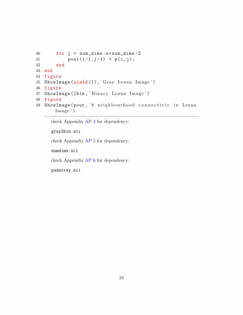
40 for j = num_dims:n+num_dims -2

41 pout(i-1,j-1) = p(i,j);

42 end

43 end

44 figure

45 ShowImage(uint8(I), ’ Gray Lenna Image ’ )46 figure

47 ShowImage(Ibin , ’ B inary Lenna Image ’ )48 figure

49 ShowImage(pout , ’ 8 ne ighbourhood c o n n e c t i v i y i n LennaImage ’ )

check Appendix AP 4 for dependency:

gray2bin.sci


numdims.sci


padarray.sci

10

Experiment: 3

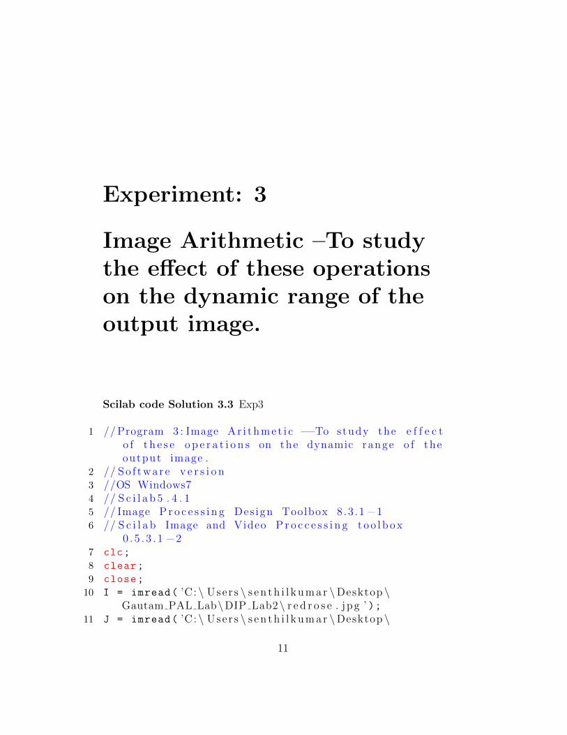
Image Arithmetic –To studythe effect of these operationson the dynamic range of theoutput image.


1 //Program 3 : Image Ar i t hme t i c −−To study the e f f e c to f t h e s e o p e r a t i o n s on the dynamic range o f theoutput image .


0 . 5 . 3 . 1 −27 clc;

8 clear;

9 close;

10 I = imread( ’C: \ User s \ s en th i l kumar \Desktop \Gautam PAL Lab\DIP Lab2\ r e d r o s e . jpg ’ );


11

Gautam PAL Lab\DIP Lab2\mistymorning . jpg ’ );12 I = imresize(I,[300 ,300] , ’ b i c u b i c ’ );13 J = imresize(J,[300 ,300] , ’ b i c u b i c ’ );14 K = imadd(I,J)

15 ShowColorImage(I, ’ Red Rose Co lo r Image ’ )16 figure

17 ShowColorImage(J, ’ Misty Morning Co lo r Image ’ )18 figure

19 ShowColorImage(K, ’ Co lo r Images a dd i t i o n r e s u l t image’ )

20 I_gray = rgb2gray(I);

21 J_gray = rgb2gray(J);

22 figure

23 ShowImage(I_gray , ’ Red Rose Gray Image ’ )24 figure

25 ShowImage(J_gray , ’ Misty Morning Gray Image ’ )26 Imean = mean2(I_gray);

27 Jmean = mean2(J_gray);

28 Ithreshold = double(Imean)/double(max(I_gray (:)));

29 Jthreshold = double(Jmean)/double(max(J_gray (:)));

30 I_bw = im2bw(I,Ithreshold);

31 J_bw = im2bw(J,Jthreshold);

32 figure

33 ShowImage(I_bw , ’ Red Rose Binary Image ’ )34 figure

35 ShowImage(J_bw , ’ Misty Morning Binary Image ’ )

12

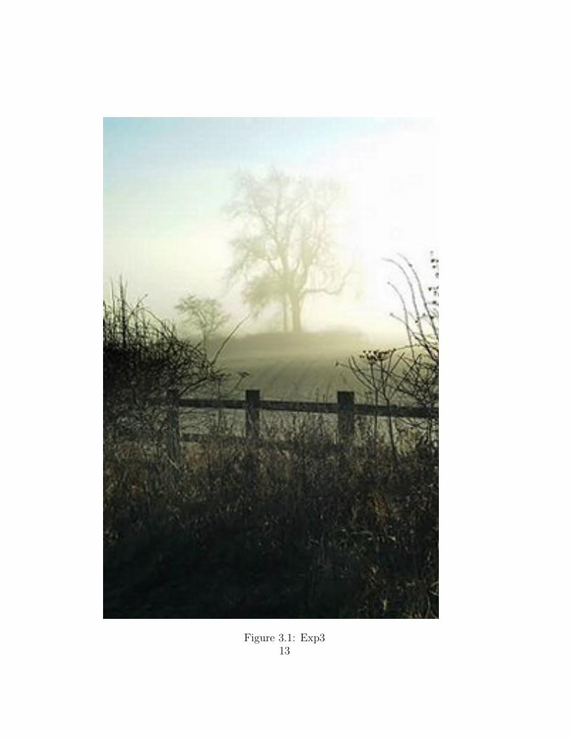
Figure 3.1: Exp313

Figure 3.2: Exp3

14

Experiment: 4

Image Arithmetic –To studymethods to enforce closureforces the output image to alsobe an 8 bit image.


1 // Prog4 . Image Ar i t hme t i c −−To study methods toe n f o r c e c l o s u r e f o r c e s the output image to a l s obe an 8 b i t image .


0 . 5 . 3 . 1 −27 clc;

8 clear;

9 close;

10 I = imread( ’C: \ User s \ s en th i l kumar \Desktop \Gautam PAL Lab\DIP Lab2\cameraman . j p e g ’ );


15

Gautam PAL Lab\DIP Lab2\ l enna . jpg ’ );12 K = imabsdiff(I,J);

13 ShowImage(I, ’ Cameraman Image ’ )14 figure

15 ShowImage(J, ’ Lenna Image ’ )16 figure

17 ShowImage(K, ’ Abso lu te D i f f e r e n c e Between cameramanand Lenna Image ’ )

18 L = imcomplement(K);

19 figure

20 ShowImage(L, ’ Complement o f d i f f e r e n c e Image K ’ )21 rect = [20 ,30 ,200 ,200];

22 I_subimage = imcrop(I,rect);

23 J_subimage = imcrop(J,rect);

24 figure

25 ShowImage(I_subimage , ’ Sub Image o f Cameraman Image ’ )26 figure

27 ShowImage(J_subimage , ’ Sub Image o f Lenna Image ’ )28 a=2;

29 b =0.5;

30 M = imlincomb(a,I,b,J);

31 figure

32 ShowImage(M, ’ L i n ea r Combination o f cameraman andLenna Image ’ )

33 N= imlincomb(b,I,a,J);

34 figure

35 ShowImage(N, ’ L i n ea r Combination o f cameraman andLenna Image ’ )

16

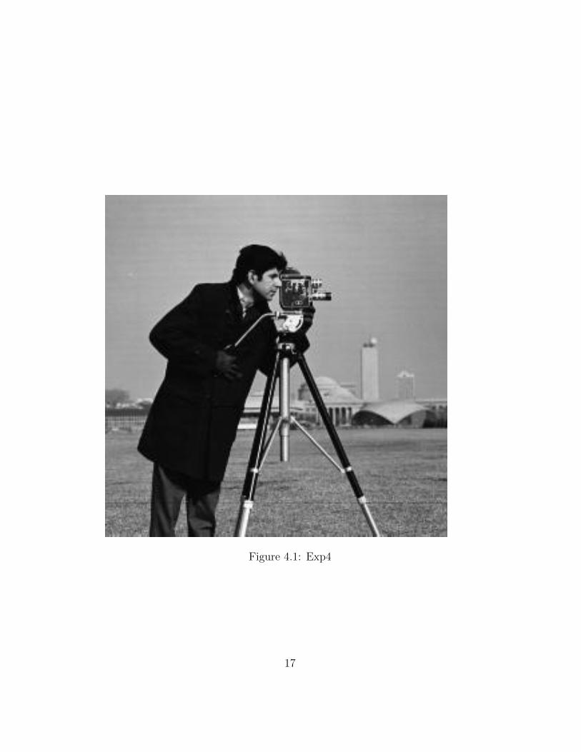
Figure 4.1: Exp4

17

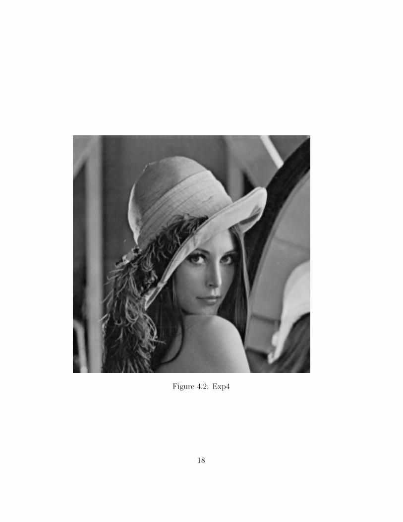
Figure 4.2: Exp4

18

Experiment: 5

Affine Transformation - Tolearn basic imagetransformation i) Translationii) Rotation iii) Scaling


1 // Prog5 . A f f i n e Trans f o rmat i on − To l e a r n b a s i cimage t r a n s f o rma t i o n

2 // i ) T r an s l a t i o n i i ) Rota t i on i i i ) S c a l i n g3 // So f twar e v e r s i o n4 //OS Windows75 // S c i l a b 5 . 4 . 16 // Image P r o c e s s i n g Des ign Toolbox 8 .3 .1 −17 // S c i l a b Image and Video P r o c c e s s i n g t o o l box

0 . 5 . 3 . 1 −28 clc;

9 clear;

10 clc;

11 I = imread( ’C: \ User s \ s en th i l kumar \Desktop \Gautam PAL Lab\DIP Lab2\ l enna . jpg ’ );// s i z e 256x256

19

12 [m,n] = size(I);

13 for i = 1:m

14 for j =1:n

15 // S c a l i n g16 J(2*i,2*j) = I(i,j);

17 // Rota t i on18 p = i*cos(%pi /2)+j*sin(%pi/2);

19 q = -i*sin(%pi /2)+j*cos(%pi/2);

20 p = ceil(abs(p)+0.0001);

21 q = ceil(abs(q)+0.0001);

22 K(p,q)= I(i,j);

23 // sh ea r t r a n s f o rma t i o n24 u = i+0.2*j;

25 v = j;

26 L(u,v)= I(i,j);

27 end

28 end

29 figure

30 ShowImage(I, ’ o r i g i n a l Image ’ );31 figure

32 ShowImage(J, ’ S c a l ed Image ’ );33 figure

34 ShowImage(K, ’ Rotated Image ’ );35 figure

36 ShowImage(L, ’ Shear t r an s f o rmed ( x d i r e c t i o n ) Image ’ );

20

Experiment: 6

Affine Transformation –Tolearn the role of interpolationoperation i) Bi-linear ii)Bi-cubic iii) nearest neighbor


1 // Prog6 . A f f i n e Trans f o rmat i on −−To l e a r n the r o l eo f i n t e r p o l a t i o n op e r a t i o n

2 // i ) Bi− l i n e a r i i ) Bi−cub i c i i i ) n e a r e s t n e i ghbo r3 // So f twar e v e r s i o n4 //OS Windows75 // S c i l a b 5 . 4 . 16 // Image P r o c e s s i n g Des ign Toolbox 8 .3 .1 −17 // S c i l a b Image and Video P r o c c e s s i n g t o o l box

0 . 5 . 3 . 1 −28 clc;

9 clear;

10 close;

11 I = imread( ’C: \ User s \ s en th i l kumar \Desktop \Gautam PAL Lab\DIP Lab2\ l enna . jpg ’ );// s i z e 256x256

21

12 [m,n] = size(I);

13 for i = 1:m

14 for j =1:n

15 // S c a l i n g16 J(1.5*i ,1.5*j) = I(i,j); // 512 x512 Image17 end

18 end

19 I_nearest = imresize(J ,[256 ,256]); // ’ n e a r e s t ’ −nea r e s t −ne i gbo r i n t e r p o l a t i o n

20 I_bilinear = imresize(J,[256 ,256] , ’ b i l i n e a r ’ );// ’b i l i n e a r ’ − b i l i n e a r i n t e r p o l a t i o n

21 I_bicubic = imresize(J,[256 ,256] , ’ b i c u b i c ’ );// ’b i cub i c ’ − b i c u b i c i n t e r p o l a t i o n

22 figure

23 ShowImage(uint8(I_nearest), ’ n e a r e s t −ne i gbo ri n t e r p o l a t i o n ’ );

24 figure

25 ShowImage(uint8(I_bilinear), ’ b i l i n e a r − b i l i n e a ri n t e r p o l a t i o n ’ );

26 figure

27 ShowImage(uint8(I_bicubic), ’ b i c u b i c − b i c u b i ci n t e r p o l a t i o n ’ );

22

Experiment: 7

Affine Transformation –Tolearn the effect of multipletransformations i) Significanceof order in which one carriedout


1 // Prog7 . A f f i n e Trans f o rmat i on −−To l e a r n the e f f e c to f mu l t i p l e t r a n s f o rma t i o n s i ) S i g n i f i c a n c e o fo r d e r i n which one c a r r i e d out


0 . 5 . 3 . 1 −27 clc;

8 clear;

9 close

10 I = imread( ’C: \ User s \ s en th i l kumar \Desktop \

23

Gautam PAL Lab\DIP Lab2\ l enna . jpg ’ );11 [m,n] = size(I);

12 for i = 1:m

13 for j =1:n

14 // sh ea r t r a n s f o rma t i o n and r o t a t i o n15 u = i+0.2*j;

16 v = 0.3*i+j;

17 M(u,v) = I(i,j);

18 // sh ea r t r an s f o rma t i on , r o t a t i o n and s c a l i n g19 N(u*1.5,v*1.5)= I(i,j);

20 end

21 end

22 figure

23 ShowImage(I, ’ o r i g i n a l Lenna Image ’ )24 figure

25 ShowImage(M, ’ Shear t r an s f o rmed+r o t a t e d Lenna Image ’ )26 figure

27 ShowImage(N, ’ Shear Transformed+r o t a t e d+s c a l e d LennaImage ’ )

24

Experiment: 8

Point Operations - To learnimage enhancement throughpoint transformation-i)Lineartransformation ii) Non-lineartransformation


1 // Prog8 . Po int Ope ra t i on s − To l e a r n imageenhancement through po i n t t r a n s f o rma t i o n

2 // i ) L in ea r t r a n s f o rma t i o n i i ) Non− l i n e a rt r a n s f o rma t i o n


0 . 5 . 3 . 1 −28 clc;

9 clear;

10 close;

25

11 I = imread( ’C: \ User s \ s en th i l kumar \Desktop \Gautam PAL Lab\DIP Lab2\ r i c e . png ’ );

12 // ( i ) . L i n ea r Trans f o rmat i on13 //IMAGE NEGATIVE14 I = double(I);

15 J = 255-I;

16 figure

17 ShowImage(I, ’ O r i g i n a l Image ’ )18 figure

19 ShowImage(J, ’ L i n ea r Trans fo rmat ion−IMAGE NEGATIVE ’ )20 // ( i i ) Non− l i n e a r t r a n s f o rma t i o n21 //GAMMA TRANSFORMATION22 GAMMA = 0.9;

23 K = I.^ GAMMA;

24 figure

25 ShowImage(K, ’Non− l i n e a r t r an s f o rma t i on −GAMMATRANSFORMATION ’ )

26

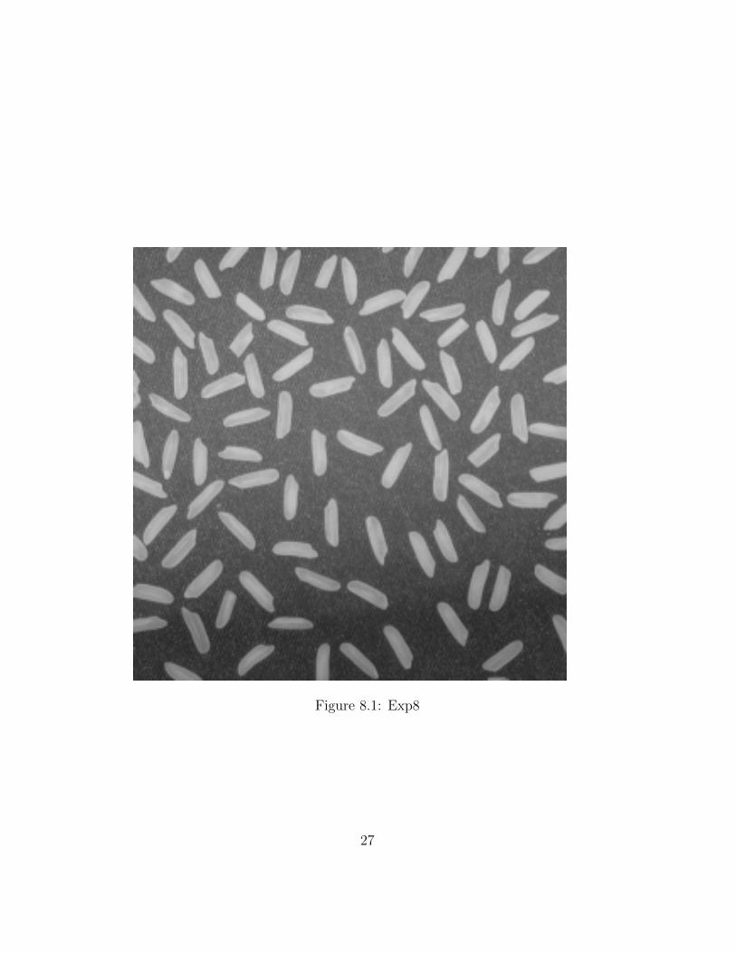
Figure 8.1: Exp8

27

Experiment: 9

Neighborhood Operations - Tolearn about neighborhoodoperations and use them for i)Linear filtering ii) Non-linearfiltering


1 // Prog9 . Neighborhood Ope ra t i on s − To l e a r n aboutne ighborhood o p e r a t i o n s and use them f o r

2 // i ) L in ea r f i l t e r i n g i i ) Non− l i n e a r f i l t e r i n g3 // So f twar e v e r s i o n4 //OS Windows75 // S c i l a b 5 . 4 . 16 // Image P r o c e s s i n g Des ign Toolbox 8 .3 .1 −17 // S c i l a b Image and Video P r o c c e s s i n g t o o l box

0 . 5 . 3 . 1 −28 clc;

9 clear;

10 close;

11 I = imread( ’C: \ User s \ s en th i l kumar \Desktop \

28

Gautam PAL Lab\DIP Lab2\ l enna . jpg ’ );12 I_noise = imnoise(I, ’ s a l t & pepper ’ );13 figure

14 ShowImage(I, ’ O r i g i n a l Lenna Image ’ )15 figure

16 ShowImage(I_noise , ’ Noisy Lenna Image ’ )17 //Case 1 : L i n ea r F i l t e r i n g18 // ( i ) . L i n ea r F i l t e r i n g −Example 1 : Average F i l t e r19 F_linear1 = 1/25* ones (5,5);// 5x5 mask20 I_linear1 = imfilter(I_noise ,F_linear1);// l i n e a r

f i l t e r i n g −Average F i l t e r21 figure

22 ShowImage(I_linear1 , ’ L i n ea r Average F i l t e r e d NoisyLenna Image ’ )

23 // ( i i ) . L i n ea r F i l t e r i n g − Example 2 : Gauss ingf i l t e r

24 hsize = [5,5];

25 sigma = 1;

26 F_linear2 = fspecial( ’ g a u s s i a n ’ , hsize , sigma); //L in ea r f i l t e r i n g − g au s s i a n F i l t e r

27 I_linear2 = imfilter(I_noise ,F_linear2);

28 figure

29 ShowImage(I_linear2 , ’ L i n ea r Gauss ian F i l t e r e d NoisyLenna Image ’ )

30 //Case 2 : Non−L inea r F i l t e r i n g31 // ( i ) . Median F i l t e r i n g32 F_NonLinear = [3,3];

33 I_NonLinear = MedianFilter(I_noise ,F_NonLinear);//Median F i l t e r 3x3

34 figure

35 ShowImage(I_NonLinear , ’ Median F i l t e r e d (Non−L inea r )Noisy Lenna Image ’ )

29

Experiment: 10

Neighborhood Operations –Tostudy the effect of the size ofneighborhood on the result ofprocessing


1 // Prog10 . Neighborhood Ope ra t i on s −−To study thee f f e c t o f the s i z e o f ne ighborhood on the r e s u l to f p r o c e s s i n g


0 . 5 . 3 . 1 −27 clc;

8 clear;

9 close;


11 I_noise = imnoise(I, ’ s a l t & pepper ’ );

30

12 FilterSize = [3 3]; // f i l t e r s i z e 3x313 I_3x3 = MedianFilter(I_noise ,FilterSize);

14 I_5x5 = MedianFilter(I_noise ,[5 5]);



17 figure


20 ShowImage(I_noise , ’ O r i g i n a l Lenna Image ’ )21 figure

22 ShowImage(I_3x3 , ’ F i l t e r e d Lenna Image−F i l t e r s i z e 3x3 ’ )

23 figure


25 figure


27 figure


31

Experiment: 11

Image Histogram - Tounderstand how frequencydistribution can be used torepresent an image.


1 // Prog11 . Image Histogram − To under s tand howf r e qu en cy d i s t r i b u t i o n can be used to r e p r e s e n tan image


0 . 5 . 3 . 1 −27 clc;

8 clear;

9 close;

10 I = imread( ’C: \ User s \ s en th i l kumar \Desktop \Gautam PAL Lab\DIP Lab2\pout . png ’ );

11 [count , cells]= imhist(I);

32

12 scf (0)

13 ShowImage(I, ’ O r i g i n a l Image pout . png ’ )14 scf (1);

15 plot2d3( ’ gnn ’ ,cells ,count)16 title( ’ Histogram Plo t o f O r i g i n a l Image ’ )17 exec( ’C: \ User s \ s en th i l kumar \Desktop \Gautam PAL Lab\

h i s t e q . s c i ’ );18 Iheq = histeq(I);

19 [count , cells]= imhist(Iheq);

20 scf (2)

21 ShowImage(Iheq , ’ Histogram Equa l i z ed Image pout . png ’ )22 scf (3)

23 plot2d3( ’ gnn ’ ,cells ,count)24 title( ’ Histogram o f Histogram Equa l i z ed Image ’ )


histeq.sci

33

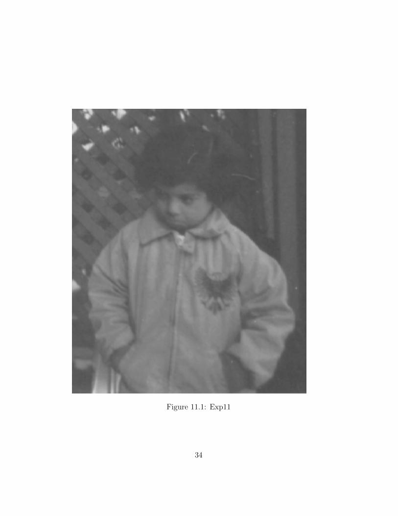
Figure 11.1: Exp11

34

Experiment: 12

Image Histogram –To study thecorrelation between the visualquality of an image with itshistogram.


1 // Prog12 . Image Histogram −−To study the c o r r e l a t i o nbetween the v i s u a l q u a l i t y o f an image with i t sh i s t og ram .


0 . 5 . 3 . 1 −27 clc;

8 clear;

9 close;

10 I = imread( ’C: \ User s \ s en th i l kumar \Desktop \Gautam PAL Lab\DIP Lab2\pout . png ’ );

11 I = imresize(I ,[256 ,256]);

35

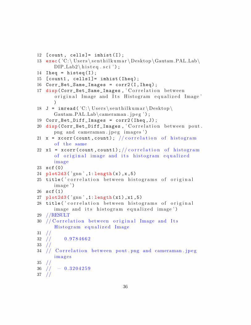
12 [count , cells]= imhist(I);

13 exec( ’C: \ User s \ s en th i l kumar \Desktop \Gautam PAL Lab\DIP Lab2\ h i s t e q . s c i ’ );

14 Iheq = histeq(I);

15 [count1 , cells1 ]= imhist(Iheq);

16 Corr_Bet_Same_Images = corr2(I,Iheq);

17 disp(Corr_Bet_Same_Images , ’ C o r r e l a t i o n betweeno r i g i n a l Image and I t s Histogram e q u a l i z e d Image ’)

18 J = imread( ’C: \ User s \ s en th i l kumar \Desktop \Gautam PAL Lab\cameraman . j p e g ’ );

19 Corr_Bet_Diff_Images = corr2(Iheq ,J);

20 disp(Corr_Bet_Diff_Images , ’ C o r r e l a t i o n between pout .png and cameraman . j p e g images ’ )

21 x = xcorr(count ,count); // c o r r e l a t i o n o f h i s t og ramo f the same

22 x1 = xcorr(count ,count1);// c o r r e l a t i o n o f h i s t og ramo f o r i g i n a l image and i t s h i s tog ram e q u a l i z e dimage

23 scf (0)

24 plot2d3( ’ gnn ’ ,1:length(x),x,5)25 title( ’ c o r r e l a t i o n between h i s t o g r ams o f o r i g i n a l

image ’ )26 scf (1)

27 plot2d3( ’ gnn ’ ,1:length(x1),x1 ,5)28 title( ’ c o r r e l a t i o n between h i s t o g r ams o f o r i g i n a l

image and i t s h i s t og ram e q u a l i z e d image ’ )29 //RESULT30 // Co r r e l a t i o n between o r i g i n a l Image and I t s

Histogram e q u a l i z e d Image31 //32 // 0 . 978466233 //34 // Co r r e l a t i o n between pout . png and cameraman . j p e g

images35 //36 // − 0 . 320425937 //

36


histeq.sci

37

Experiment: 13

Fourier Transform: Tounderstand some of thefundamental properties of theFourier transform.


1 // Prog13 . Fou r i e r Transform : To under s tand some o fthe fundamenta l p r o p e r t i e s o f the Fou r i e rt r an s f o rm .


0 . 5 . 3 . 1 −27 clc;

8 clear;

9 close;


11 exec( ’C: \ User s \ s en th i l kumar \Desktop \Gautam PAL Lab\

38

DIP Lab2\ f f t 2 d . s c i ’ );12 exec( ’C: \ User s \ s en th i l kumar \Desktop \Gautam PAL Lab\

DIP Lab2\ i f f t 2 d . s c i ’ );13 // [ 1 ] . 2D−DFT and i t s I n v e r s e 2D−DFT14 I = double(I);

15 J = fft2d(I);

16 K = real(ifft2d(J));

17 figure


20 ShowImage(abs(J), ’ 2D DFT ( spectrum ) o f Lenna Image ’ )21 figure

22 ShowImage(K, ’ 2d IDFT o f Lenna Image ’ )23 // [ 2 ] . Two t imes f f t s h i f t r e s u l t s i n o r i g i n a l

spectrum24 L = fftshift(J);

25 M = fftshift(L);

26 figure

27 ShowImage(abs(L), ’ f f t s h i t e d spectrum o f Lenna Image ’)

28 figure

29 ShowImage(abs(M), ’ two t imes f f t s h i f t e d ’ )


fft2d.sci


ifft2d.sci

39

Experiment: 14

Colour Image Processing: Tolearn colour images are handledand processed i)Models forrepresenting colour ii) Methodsof proces


1 // Prog14 . Colour Image P r o c e s s i n g : To l e a r n c o l o u rimages a r e handled and p r o c e s s e d

2 // i ) Models f o r r e p r e s e n t i n g c o l o u r i i ) Methods o fp r o c e s


0 . 5 . 3 . 1 −28 clc;

9 clear;

10 close;

40

11 RGB = imread( ’C: \ User s \ s en th i l kumar \Desktop \Gautam PAL Lab\DIP lab2 \ f o o t b a l l . j pg ’ );

12 figure

13 ShowColorImage(RGB , ’RGB Color Image ’ )14 YIQ = rgb2ntsc(RGB);

15 figure

16 ShowColorImage(YIQ , ’NTSC image YIQ ’ )17 RGB = ntsc2rgb(YIQ);

18 YCC = rgb2ycbcr(RGB);

19 figure

20 ShowColorImage(YCC , ’ e q u i v a l e n t HSV image YCbCr ’ )21 RGB = ycbcr2rgb(YCC);

22 HSV = rgb2hsv(RGB);

23 figure

24 ShowColorImage(HSV , ’ e q u i v a l e n t HSV image ’ )25 RGB = hsv2rgb(HSV);

26 R = RGB(:,:,1);

27 G = RGB(:,:,2);

28 B = RGB(:,:,3);

29 figure

30 ShowImage(R, ’ Red Matr ix ’ )31 figure

32 ShowImage(G, ’ Green Matr ix ’ )33 figure

34 ShowImage(B, ’ Blue Matr ix ’ )

41

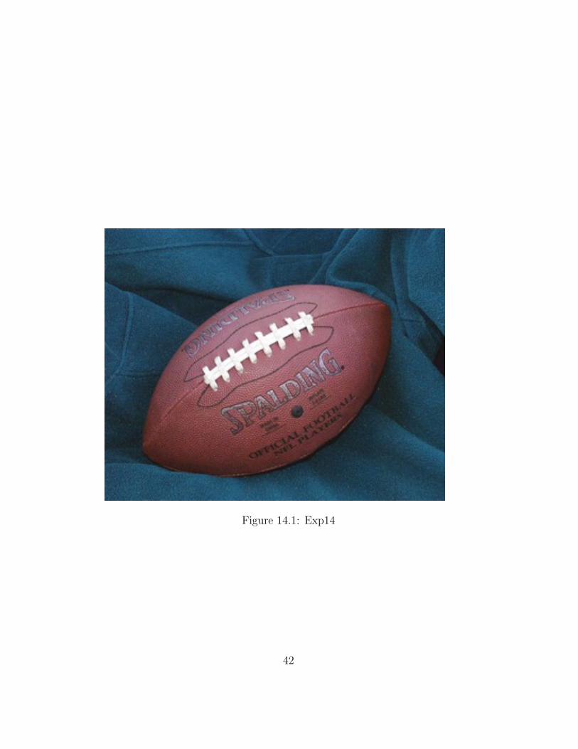
Figure 14.1: Exp14

42

Experiment: 15

Morphological Operations: Tounderstand the basics ofmorphological operations whichare used in analyzing the formand shape de


1 // Prog15 . Morpho l o g i c a l Ope ra t i on s : To under s tand theb a s i c s o f mo rpho l o g i c a l o p e r a t i o n s

2 // which a r e used i n an a l y z i n g the form and shape3 // So f twar e v e r s i o n4 //OS Windows75 // S c i l a b 5 . 4 . 16 // Image P r o c e s s i n g Des ign Toolbox 8 .3 .1 −17 // S c i l a b Image and Video P r o c c e s s i n g t o o l box

0 . 5 . 3 . 1 −28 clc;

9 clear;

10 close;

11 Image = imread( ’C: \ User s \ s en th i l kumar \Desktop \

43

Gautam PAL Lab\DIP Lab2\ t i r e . j p e g ’ );12 StructureElement = CreateStructureElement( ’ s qua r e ’

,3); // g en e r a t e s t r u c t u r i n g e l ement IPD atom13 ResultImage1 = ErodeImage(Image ,StructureElement);

//IPD Atom14 ResultImage2 = DilateImage(Image ,StructureElement);

//IPD Atom15 ResultImage3 = BottomHat(Image ,StructureElement);

//IPD Atom16 ResultImage4 = TopHat(Image ,StructureElement); //

IPD Atom17 figure

18 ShowImage(Image , ’ O r i g i n a l Image ’ )19 figure

20 ShowImage(ResultImage1 , ’ Eroded Image ’ )21 figure

22 ShowImage(ResultImage2 , ’ D i l a t e d Image ’ )23 figure

24 ShowImage(ResultImage3 , ’ bottom hat f i l t e r e d image ’ )25 figure

26 ShowImage(ResultImage4 , ’ top hat f i l t e r e d image ’ )27

28 ResultImage5 = imadd(ResultImage3 ,ResultImage4);

29 figure

30 ShowImage(ResultImage4 , ’ top hat f i l t e r e d image+bottom hat f i l t e r e d image ’ )

44

Figure 15.1: Exp15

45

Appendix

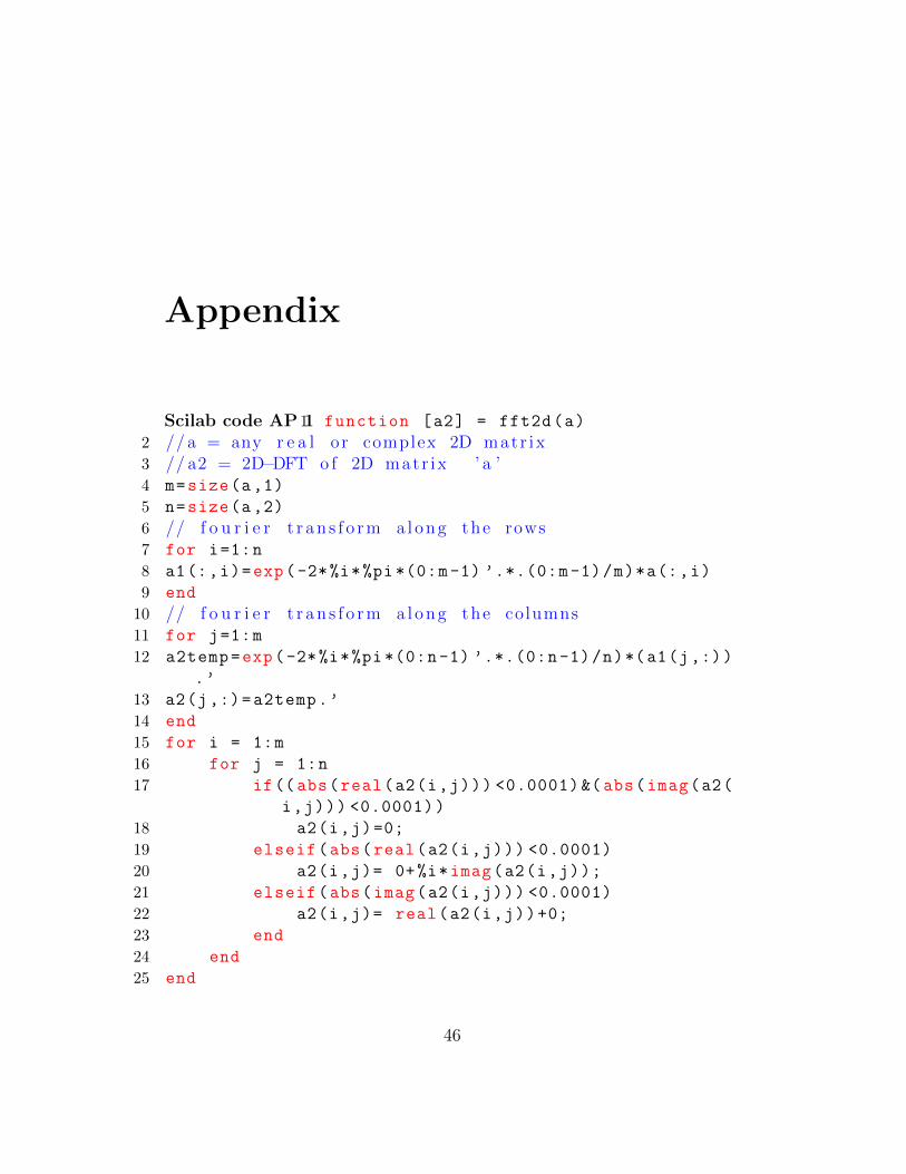
Scilab code AP 11 function [a2] = fft2d(a)

2 // a = any r e a l o r complex 2D matr ix3 // a2 = 2D−DFT o f 2D matr ix ’ a ’4 m=size(a,1)

5 n=size(a,2)

6 // f o u r i e r t r an s f o rm a long the rows7 for i=1:n

8 a1(:,i)=exp(-2*%i*%pi *(0:m-1) ’.*.(0:m-1)/m)*a(:,i)

9 end

10 // f o u r i e r t r an s f o rm a long the columns11 for j=1:m

12 a2temp=exp(-2*%i*%pi *(0:n-1) ’.*.(0:n-1)/n)*(a1(j,:))

.’

13 a2(j,:)=a2temp.’

14 end

15 for i = 1:m

16 for j = 1:n

17 if((abs(real(a2(i,j))) <0.0001)&(abs(imag(a2(

i,j))) <0.0001))

18 a2(i,j)=0;

19 elseif(abs(real(a2(i,j))) <0.0001)

20 a2(i,j)= 0+%i*imag(a2(i,j));

21 elseif(abs(imag(a2(i,j))) <0.0001)

22 a2(i,j)= real(a2(i,j))+0;

23 end

24 end

25 end

46

2D Fast Fourier Trasnform

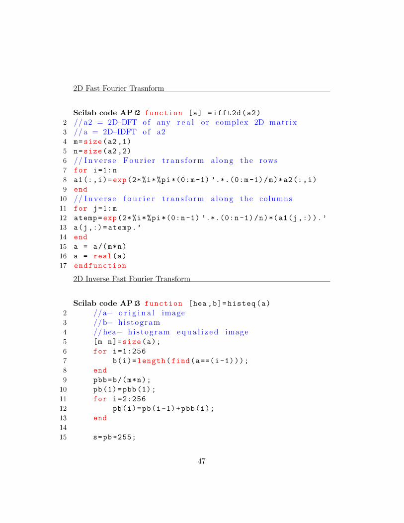
Scilab code AP 21 function [a] =ifft2d(a2)

2 // a2 = 2D−DFT o f any r e a l o r complex 2D matr ix3 // a = 2D−IDFT o f a24 m=size(a2 ,1)

5 n=size(a2 ,2)

6 // I n v e r s e Fou r i e r t r an s f o rm a long the rows7 for i=1:n

8 a1(:,i)=exp(2*%i*%pi *(0:m-1) ’.*.(0:m-1)/m)*a2(:,i)

9 end

10 // I n v e r s e f o u r i e r t r an s f o rm a long the columns11 for j=1:m

12 atemp=exp (2*%i*%pi *(0:n-1) ’.*.(0:n-1)/n)*(a1(j,:)).’

13 a(j,:)=atemp.’

14 end

15 a = a/(m*n)

16 a = real(a)

17 endfunction

2D Inverse Fast Fourier Transform

Scilab code AP 31 function [hea ,b]= histeq(a)

2 //a− o r i g i n a l image3 //b− h i s tog ram4 // hea− h i s tog ram e q u a l i z e d image5 [m n]=size(a);

6 for i=1:256

7 b(i)=length(find(a==(i-1)));

8 end

9 pbb=b/(m*n);

10 pb(1)=pbb (1);

11 for i=2:256

12 pb(i)=pb(i-1)+pbb(i);

13 end

14

15 s=pb*255;

47

16 sb=uint8(round(s));

17 index =0;

18 for i=1:m

19 for j=1:n

20 index = double(a(i,j))+1; // c onve r t i t todoub le

21 // o t h e rw i s e index = 255+1 =022 hea(i,j)= sb(index);// h i s tog ram

e q u a l i z a t i o n23 end

24 end

25 endfunction

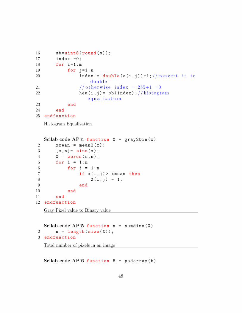
Histogram Equalization

Scilab code AP 41 function X = gray2bin(x)

2 xmean = mean2(x);

3 [m,n]= size(x);

4 X = zeros(m,n);

5 for i = 1:m

6 for j = 1:n

7 if x(i,j)> xmean then

8 X(i,j) = 1;

9 end

10 end

11 end

12 endfunction

Gray Pixel value to Binary value

Scilab code AP 51 function n = numdims(X)

2 n = length(size(X));

3 endfunction

Total number of pixels in an image

Scilab code AP 61 function B = padarray(b)

48

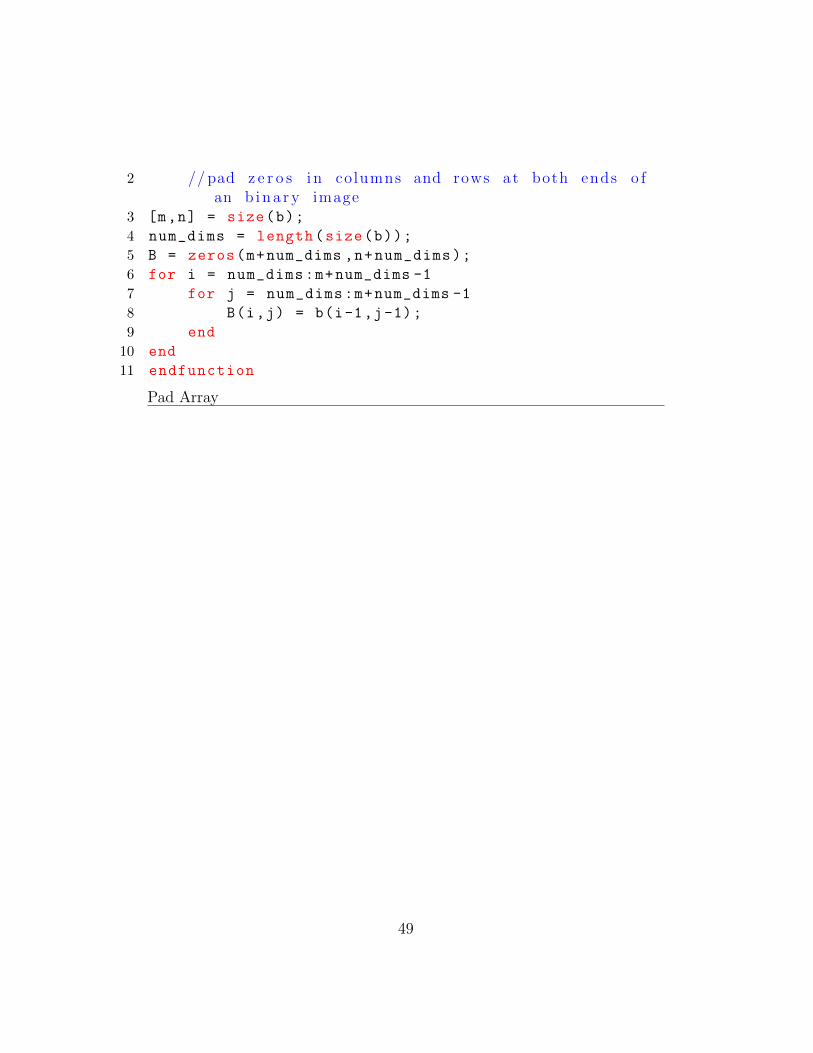
2 //pad z e r o s i n columns and rows at both ends o fan b ina ry image

3 [m,n] = size(b);

4 num_dims = length(size(b));

5 B = zeros(m+num_dims ,n+num_dims);

6 for i = num_dims:m+num_dims -1

7 for j = num_dims:m+num_dims -1

8 B(i,j) = b(i-1,j-1);

9 end

10 end

11 endfunction

Pad Array

49

Scilab Manual for Image Processing by Mr Gautam Pal ...

Documents