Ordinary Differential Equations Numerical Solution of ODEs Additional Numerical Methods Scientific Computing: An Introductory Survey Chapter 9 – Initial Value Problems for Ordinary Differential Equations Prof. Michael T. Heath Department of Computer Science University of Illinois at Urbana-Champaign Copyright c 2002. Reproduction permitted for noncommercial, educational use only. Michael T. Heath Scientific Computing 1 / 84

Welcome message from author
This document is posted to help you gain knowledge. Please leave a comment to let me know what you think about it! Share it to your friends and learn new things together.
Transcript
Ordinary Differential EquationsNumerical Solution of ODEs
Additional Numerical Methods
Scientific Computing: An Introductory SurveyChapter 9 – Initial Value Problems for
Ordinary Differential Equations
Prof. Michael T. Heath
Department of Computer ScienceUniversity of Illinois at Urbana-Champaign
Copyright c© 2002. Reproduction permittedfor noncommercial, educational use only.
Michael T. Heath Scientific Computing 1 / 84
Ordinary Differential EquationsNumerical Solution of ODEs
Additional Numerical Methods
Outline
1 Ordinary Differential Equations
2 Numerical Solution of ODEs
3 Additional Numerical Methods
Michael T. Heath Scientific Computing 2 / 84
Ordinary Differential EquationsNumerical Solution of ODEs
Additional Numerical Methods
Differential EquationsInitial Value ProblemsStability
Differential Equations
Differential equations involve derivatives of unknownsolution function
Ordinary differential equation (ODE): all derivatives arewith respect to single independent variable, oftenrepresenting time
Solution of differential equation is function ininfinite-dimensional space of functions
Numerical solution of differential equations is based onfinite-dimensional approximation
Differential equation is replaced by algebraic equationwhose solution approximates that of given differentialequation
Michael T. Heath Scientific Computing 3 / 84
Ordinary Differential EquationsNumerical Solution of ODEs
Additional Numerical Methods
Differential EquationsInitial Value ProblemsStability
Order of ODE
Order of ODE is determined by highest-order derivative ofsolution function appearing in ODE
ODE with higher-order derivatives can be transformed intoequivalent first-order system
We will discuss numerical solution methods only forfirst-order ODEs
Most ODE software is designed to solve only first-orderequations
Michael T. Heath Scientific Computing 4 / 84

Ordinary Differential EquationsNumerical Solution of ODEs
Additional Numerical Methods
Differential EquationsInitial Value ProblemsStability
Higher-Order ODEs, continued
For k-th order ODE
y(k)(t) = f(t, y, y′, . . . , y(k−1))
define k new unknown functions
u1(t) = y(t), u2(t) = y′(t), . . . , uk(t) = y(k−1)(t)
Then original ODE is equivalent to first-order systemu′1(t)u′2(t)
...u′k−1(t)
u′k(t)
=
u2(t)u3(t)
...uk(t)
f(t, u1, u2, . . . , uk)
Michael T. Heath Scientific Computing 5 / 84

Ordinary Differential EquationsNumerical Solution of ODEs
Additional Numerical Methods
Differential EquationsInitial Value ProblemsStability
Example: Newton’s Second Law
Newton’s Second Law of Motion, F = ma, is second-orderODE, since acceleration a is second derivative of positioncoordinate, which we denote by y
Thus, ODE has form
y′′ = F/m
where F and m are force and mass, respectively
Defining u1 = y and u2 = y′ yields equivalent system oftwo first-order ODEs [
u′1u′2
]=
[u2F/m
]Michael T. Heath Scientific Computing 6 / 84
Ordinary Differential EquationsNumerical Solution of ODEs
Additional Numerical Methods
Differential EquationsInitial Value ProblemsStability
Example, continued
We can now use methods for first-order equations to solvethis system
First component of solution u1 is solution y of originalsecond-order equation
Second component of solution u2 is velocity y′
Michael T. Heath Scientific Computing 7 / 84
Ordinary Differential EquationsNumerical Solution of ODEs
Additional Numerical Methods
Differential EquationsInitial Value ProblemsStability
Ordinary Differential Equations
General first-order system of ODEs has form
y′(t) = f(t,y)
where y : R→ Rn, f : Rn+1 → Rn, and y′ = dy/dt denotesderivative with respect to t,
y′1(t)y′2(t)
...y′n(t)
=
dy1(t)/dtdy2(t)/dt
...dyn(t)/dt
Function f is given and we wish to determine unknownfunction y satisfying ODE
For simplicity, we will often consider special case of singlescalar ODE, n = 1
Michael T. Heath Scientific Computing 8 / 84

Ordinary Differential EquationsNumerical Solution of ODEs
Additional Numerical Methods
Differential EquationsInitial Value ProblemsStability
Initial Value Problems
By itself, ODE y′ = f(t,y) does not determine uniquesolution function
This is because ODE merely specifies slope y′(t) ofsolution function at each point, but not actual value y(t) atany point
Infinite family of functions satisfies ODE, in general,provided f is sufficiently smooth
To single out particular solution, value y0 of solutionfunction must be specified at some point t0
Michael T. Heath Scientific Computing 9 / 84

Ordinary Differential EquationsNumerical Solution of ODEs
Additional Numerical Methods
Differential EquationsInitial Value ProblemsStability
Initial Value Problems, continued
Thus, part of given problem data is requirement thaty(t0) = y0, which determines unique solution to ODE
Because of interpretation of independent variable t astime, think of t0 as initial time and y0 as initial value
Hence, this is termed initial value problem, or IVP
ODE governs evolution of system in time from its initialstate y0 at time t0 onward, and we seek function y(t) thatdescribes state of system as function of time
Michael T. Heath Scientific Computing 10 / 84

Ordinary Differential EquationsNumerical Solution of ODEs
Additional Numerical Methods
Differential EquationsInitial Value ProblemsStability
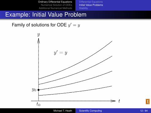
Example: Initial Value Problem
Consider scalar ODEy′ = y
Family of solutions is given by y(t) = c et, where c is anyreal constant
Imposing initial condition y(t0) = y0 singles out uniqueparticular solution
For this example, if t0 = 0, then c = y0, which means thatsolution is y(t) = y0e
t
Michael T. Heath Scientific Computing 11 / 84
Ordinary Differential EquationsNumerical Solution of ODEs
Additional Numerical Methods
Differential EquationsInitial Value ProblemsStability
Example: Initial Value Problem
Family of solutions for ODE y′ = y
Michael T. Heath Scientific Computing 12 / 84

Ordinary Differential EquationsNumerical Solution of ODEs
Additional Numerical Methods
Differential EquationsInitial Value ProblemsStability
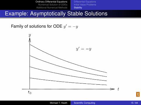
Stability of Solutions
Solution of ODE is
Stable if solutions resulting from perturbations of initialvalue remain close to original solution
Asymptotically stable if solutions resulting fromperturbations converge back to original solution
Unstable if solutions resulting from perturbations divergeaway from original solution without bound
Michael T. Heath Scientific Computing 13 / 84

Ordinary Differential EquationsNumerical Solution of ODEs
Additional Numerical Methods
Differential EquationsInitial Value ProblemsStability
Example: Stable Solutions
Family of solutions for ODE y′ = 12
Michael T. Heath Scientific Computing 14 / 84
Ordinary Differential EquationsNumerical Solution of ODEs
Additional Numerical Methods
Differential EquationsInitial Value ProblemsStability
Example: Asymptotically Stable Solutions
Family of solutions for ODE y′ = −y
Michael T. Heath Scientific Computing 15 / 84
Ordinary Differential EquationsNumerical Solution of ODEs
Additional Numerical Methods
Differential EquationsInitial Value ProblemsStability
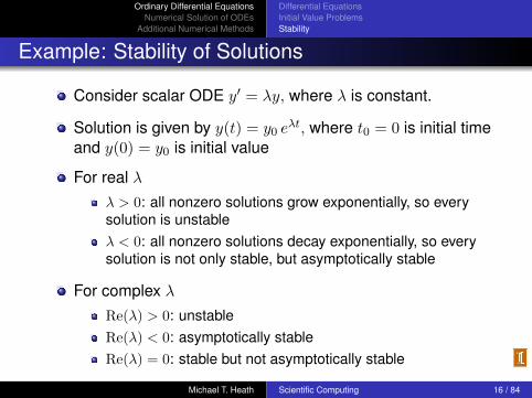
Example: Stability of Solutions
Consider scalar ODE y′ = λy, where λ is constant.
Solution is given by y(t) = y0 eλt, where t0 = 0 is initial time
and y(0) = y0 is initial value
For real λλ > 0: all nonzero solutions grow exponentially, so everysolution is unstableλ < 0: all nonzero solutions decay exponentially, so everysolution is not only stable, but asymptotically stable
For complex λRe(λ) > 0: unstableRe(λ) < 0: asymptotically stableRe(λ) = 0: stable but not asymptotically stable
Michael T. Heath Scientific Computing 16 / 84
Ordinary Differential EquationsNumerical Solution of ODEs
Additional Numerical Methods
Differential EquationsInitial Value ProblemsStability
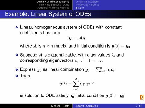
Example: Linear System of ODEs
Linear, homogeneous system of ODEs with constantcoefficients has form
y′ = Ay
where A is n× n matrix, and initial condition is y(0) = y0
Suppose A is diagonalizable, with eigenvalues λi andcorresponding eigenvectors vi, i = 1, . . . , n
Express y0 as linear combination y0 =∑n
i=1 αivi
Then
y(t) =n∑i=1
αivieλit
is solution to ODE satisfying initial condition y(0) = y0
Michael T. Heath Scientific Computing 17 / 84
Ordinary Differential EquationsNumerical Solution of ODEs
Additional Numerical Methods
Differential EquationsInitial Value ProblemsStability
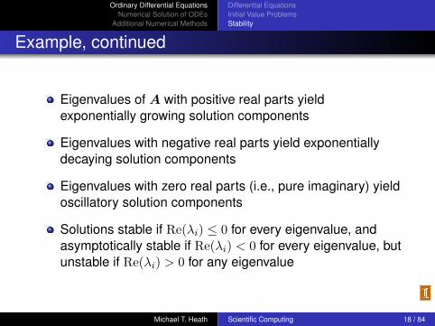
Example, continued
Eigenvalues of A with positive real parts yieldexponentially growing solution components
Eigenvalues with negative real parts yield exponentiallydecaying solution components
Eigenvalues with zero real parts (i.e., pure imaginary) yieldoscillatory solution components
Solutions stable if Re(λi) ≤ 0 for every eigenvalue, andasymptotically stable if Re(λi) < 0 for every eigenvalue, butunstable if Re(λi) > 0 for any eigenvalue
Michael T. Heath Scientific Computing 18 / 84
Ordinary Differential EquationsNumerical Solution of ODEs
Additional Numerical Methods
Differential EquationsInitial Value ProblemsStability
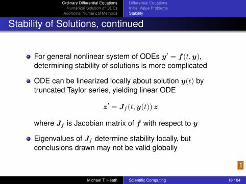
Stability of Solutions, continued
For general nonlinear system of ODEs y′ = f(t,y),determining stability of solutions is more complicated
ODE can be linearized locally about solution y(t) bytruncated Taylor series, yielding linear ODE
z′ = Jf (t,y(t)) z
where Jf is Jacobian matrix of f with respect to y
Eigenvalues of Jf determine stability locally, butconclusions drawn may not be valid globally
Michael T. Heath Scientific Computing 19 / 84
Ordinary Differential EquationsNumerical Solution of ODEs
Additional Numerical Methods
Euler’s MethodAccuracy and StabilityImplicit Methods and Stiffness
Numerical Solution of ODEs
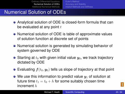
Analytical solution of ODE is closed-form formula that canbe evaluated at any point t
Numerical solution of ODE is table of approximate valuesof solution function at discrete set of points
Numerical solution is generated by simulating behavior ofsystem governed by ODE
Starting at t0 with given initial value y0, we track trajectorydictated by ODE
Evaluating f(t0,y0) tells us slope of trajectory at that point
We use this information to predict value y1 of solution atfuture time t1 = t0 + h for some suitably chosen timeincrement h
Michael T. Heath Scientific Computing 20 / 84

Ordinary Differential EquationsNumerical Solution of ODEs
Additional Numerical Methods
Euler’s MethodAccuracy and StabilityImplicit Methods and Stiffness
Numerical Solution of ODEs, continued
Approximate solution values are generated step by step inincrements moving across interval in which solution issought
In stepping from one discrete point to next, we incur someerror, which means that next approximate solution valuelies on different solution from one we started on
Stability or instability of solutions determines, in part,whether such errors are magnified or diminished with time
Michael T. Heath Scientific Computing 21 / 84

Ordinary Differential EquationsNumerical Solution of ODEs
Additional Numerical Methods
Euler’s MethodAccuracy and StabilityImplicit Methods and Stiffness
Euler’s MethodFor general system of ODEs y′ = f(t,y), consider Taylorseries
y(t+ h) = y(t) + hy′(t) +h2
2y′′(t) + · · ·
= y(t) + hf(t,y(t)) +h2
2y′′(t) + · · ·
Euler’s method results from dropping terms of second andhigher order to obtain approximate solution value
yk+1 = yk + hkf(tk,yk)
Euler’s method advances solution by extrapolating alongstraight line whose slope is given by f(tk,yk)
Euler’s method is single-step method because it dependson information at only one point in time to advance to nextpoint
Michael T. Heath Scientific Computing 22 / 84

Ordinary Differential EquationsNumerical Solution of ODEs
Additional Numerical Methods
Euler’s MethodAccuracy and StabilityImplicit Methods and Stiffness
Example: Euler’s Method
Applying Euler’s method to ODE y′ = y with step size h, weadvance solution from time t0 = 0 to time t1 = t0 + h
y1 = y0 + hy′0 = y0 + hy0 = (1 + h)y0
Value for solution we obtain at t1 is not exact, y1 6= y(t1)
For example, if t0 = 0, y0 = 1, and h = 0.5, then y1 = 1.5,whereas exact solution for this initial value isy(0.5) = exp(0.5) ≈ 1.649
Thus, y1 lies on different solution from one we started on
Michael T. Heath Scientific Computing 23 / 84
Ordinary Differential EquationsNumerical Solution of ODEs
Additional Numerical Methods
Euler’s MethodAccuracy and StabilityImplicit Methods and Stiffness
Example, continued
To continue numerical solution process, we take anotherstep from t1 to t2 = t1 + h = 1.0, obtainingy2 = y1 + hy1 = 1.5 + (0.5)(1.5) = 2.25
Now y2 differs not only from true solution of originalproblem at t = 1, y(1) = exp(1) ≈ 2.718, but it also differsfrom solution through previous point (t1, y1), which hasapproximate value 2.473 at t = 1
Thus, we have moved to still another solution for this ODE
Michael T. Heath Scientific Computing 24 / 84
Ordinary Differential EquationsNumerical Solution of ODEs
Additional Numerical Methods
Euler’s MethodAccuracy and StabilityImplicit Methods and Stiffness
Example, continued
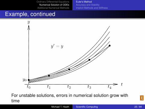
For unstable solutions, errors in numerical solution grow withtime
Michael T. Heath Scientific Computing 25 / 84

Ordinary Differential EquationsNumerical Solution of ODEs
Additional Numerical Methods
Euler’s MethodAccuracy and StabilityImplicit Methods and Stiffness
Example, continued
For stable solutions, errors in numerical solution may diminishwith time
< interactive example >Michael T. Heath Scientific Computing 26 / 84

Ordinary Differential EquationsNumerical Solution of ODEs
Additional Numerical Methods
Euler’s MethodAccuracy and StabilityImplicit Methods and Stiffness
Errors in Numerical Solution of ODEs
Numerical methods for solving ODEs incur two distincttypes of error
Rounding error, which is due to finite precision offloating-point arithmeticTruncation error (discretization error ), which is due toapproximation method used and would remain even if allarithmetic were exact
In practice, truncation error is dominant factor determiningaccuracy of numerical solutions of ODEs, so we willhenceforth ignore rounding error
Michael T. Heath Scientific Computing 27 / 84
Ordinary Differential EquationsNumerical Solution of ODEs
Additional Numerical Methods
Euler’s MethodAccuracy and StabilityImplicit Methods and Stiffness
Global Error and Local Error
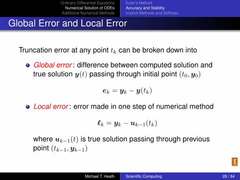
Truncation error at any point tk can be broken down into
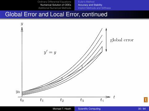
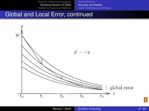
Global error : difference between computed solution andtrue solution y(t) passing through initial point (t0,y0)
ek = yk − y(tk)
Local error : error made in one step of numerical method
`k = yk − uk−1(tk)
where uk−1(t) is true solution passing through previouspoint (tk−1,yk−1)
Michael T. Heath Scientific Computing 28 / 84
Ordinary Differential EquationsNumerical Solution of ODEs
Additional Numerical Methods
Euler’s MethodAccuracy and StabilityImplicit Methods and Stiffness
Global Error and Local Error, continued
Global error is not necessarily sum of local errors
Global error is generally greater than sum of local errors ifsolutions are unstable, but may be less than sum ifsolutions are stable
Having small global error is what we want, but we cancontrol only local error directly
Michael T. Heath Scientific Computing 29 / 84
Ordinary Differential EquationsNumerical Solution of ODEs
Additional Numerical Methods
Euler’s MethodAccuracy and StabilityImplicit Methods and Stiffness
Global Error and Local Error, continued
Michael T. Heath Scientific Computing 30 / 84
Ordinary Differential EquationsNumerical Solution of ODEs
Additional Numerical Methods
Euler’s MethodAccuracy and StabilityImplicit Methods and Stiffness
Global and Local Error, continued
Michael T. Heath Scientific Computing 31 / 84
Ordinary Differential EquationsNumerical Solution of ODEs
Additional Numerical Methods
Euler’s MethodAccuracy and StabilityImplicit Methods and Stiffness
Order of Accuracy
Order of accuracy of numerical method is p if
`k = O(hp+1k )
Then local error per unit step, `k/hk = O(hpk)
Under reasonable conditions, ek = O(hp), where h isaverage step size
< interactive example >
Michael T. Heath Scientific Computing 32 / 84

Ordinary Differential EquationsNumerical Solution of ODEs
Additional Numerical Methods
Euler’s MethodAccuracy and StabilityImplicit Methods and Stiffness
Stability
Numerical method is stable if small perturbations do notcause resulting numerical solutions to diverge from eachother without bound
Such divergence of numerical solutions could be causedby instability of solution to ODE, but can also be due tonumerical method itself, even when solutions to ODE arestable
Michael T. Heath Scientific Computing 33 / 84
Ordinary Differential EquationsNumerical Solution of ODEs
Additional Numerical Methods
Euler’s MethodAccuracy and StabilityImplicit Methods and Stiffness
Determining Stability and Accuracy
Simple approach to determining stability and accuracy ofnumerical method is to apply it to scalar ODE y′ = λy,where λ is (possibly complex) constant
Exact solution is given by y(t) = y0eλt, where y(0) = y0 is
initial condition
Determine stability of numerical method by characterizinggrowth of numerical solution
Determine accuracy of numerical method by comparingexact and numerical solutions
Michael T. Heath Scientific Computing 34 / 84
Ordinary Differential EquationsNumerical Solution of ODEs
Additional Numerical Methods
Euler’s MethodAccuracy and StabilityImplicit Methods and Stiffness
Example: Euler’s Method
Applying Euler’s method to y′ = λy using fixed step size h,
yk+1 = yk + hλyk = (1 + hλ)yk
which means that
yk = (1 + hλ)ky0
If Re(λ) < 0, exact solution decays to zero as t increases,as does computed solution if
|1 + hλ| < 1
which holds if hλ lies inside circle in complex plane ofradius 1 centered at −1
< interactive example >
Michael T. Heath Scientific Computing 35 / 84
Ordinary Differential EquationsNumerical Solution of ODEs
Additional Numerical Methods
Euler’s MethodAccuracy and StabilityImplicit Methods and Stiffness
Euler’s Method, continued
If λ is real, then hλ must lie in interval (−2, 0), so for λ < 0,we must have
h ≤ − 2
λ
for Euler’s method to be stable
Growth factor 1 + hλ agrees with series expansion
ehλ = 1 + hλ+(hλ)2
2+
(hλ)3
6+ · · ·
through terms of first order in h, so Euler’s method isfirst-order accurate
Michael T. Heath Scientific Computing 36 / 84
Ordinary Differential EquationsNumerical Solution of ODEs
Additional Numerical Methods
Euler’s MethodAccuracy and StabilityImplicit Methods and Stiffness
Euler’s Method, continued
For general system of ODEs y′ = f(t,y), consider Taylorseries
y(t+ h) = y(t) + hy′(t) +O(h2)= y(t) + hf(t,y(t)) +O(h2)
If we take t = tk and h = hk, we obtain
y(tk+1) = y(tk) + hkf(tk,y(tk)) +O(h2k)
Subtracting this from Euler’s method,
ek+1 = yk+1 − y(tk+1)
= [yk − y(tk)] + hk[f(tk,yk)− f(tk,y(tk))]−O(h2k)
Michael T. Heath Scientific Computing 37 / 84
Ordinary Differential EquationsNumerical Solution of ODEs
Additional Numerical Methods
Euler’s MethodAccuracy and StabilityImplicit Methods and Stiffness
Euler’s Method, continued
If there were no prior errors, then we would haveyk = y(tk), and differences in brackets on right side wouldbe zero, leaving only O(h2k) term, which is local error
This means that Euler’s method is first-order accurate
Michael T. Heath Scientific Computing 38 / 84
Ordinary Differential EquationsNumerical Solution of ODEs
Additional Numerical Methods
Euler’s MethodAccuracy and StabilityImplicit Methods and Stiffness
Euler’s Method, continued
From previous derivation, global error is sum of local errorand propagated errorFrom Mean Value Theorem,
f(tk,yk)− f(tk,y(tk)) = Jf (tk, ξ)(yk − y(tk))
for some (unknown) value ξ, where Jf is Jacobian matrixof f with respect to ySo we can express global error at step k + 1 as
ek+1 = (I + hkJf )ek + `k+1
Thus, global error is multiplied at each step by growthfactor I + hkJfErrors do not grow if spectral radius ρ(I + hkJf ) ≤ 1,which holds if all eigenvalues of hkJf lie inside circle incomplex plane of radius 1 centered at −1
Michael T. Heath Scientific Computing 39 / 84

Ordinary Differential EquationsNumerical Solution of ODEs
Additional Numerical Methods
Euler’s MethodAccuracy and StabilityImplicit Methods and Stiffness
Stability of Numerical Methods for ODEs
In general, growth factor depends on
Numerical method, which determines form of growth factor
Step size h
Jacobian Jf , which is determined by particular ODE
Michael T. Heath Scientific Computing 40 / 84
Ordinary Differential EquationsNumerical Solution of ODEs
Additional Numerical Methods
Euler’s MethodAccuracy and StabilityImplicit Methods and Stiffness
Step Size Selection
In choosing step size for advancing numerical solution ofODE, we want to take large steps to reduce computationalcost, but must also take into account both stability andaccuracy
To yield meaningful solution, step size must obey anystability restrictions
In addition, local error estimate is needed to ensure thatdesired accuracy is achieved
With Euler’s method, for example, local error isapproximately (h2k/2)y
′′, so choose step size to satisfy
hk ≤√2 tol/‖y′′‖
Michael T. Heath Scientific Computing 41 / 84

Ordinary Differential EquationsNumerical Solution of ODEs
Additional Numerical Methods
Euler’s MethodAccuracy and StabilityImplicit Methods and Stiffness
Step Size Selection, continued
We do not know value of y′′, but we can estimate it bydifference quotient
y′′ ≈y′k − y′k−1tk − tk−1
Other methods of obtaining error estimates are based ondifference between results obtained using methods ofdifferent orders or different step sizes
Michael T. Heath Scientific Computing 42 / 84

Ordinary Differential EquationsNumerical Solution of ODEs
Additional Numerical Methods
Euler’s MethodAccuracy and StabilityImplicit Methods and Stiffness
Implicit Methods
Euler’s method is explicit in that it uses only information attime tk to advance solution to time tk+1
This may seem desirable, but Euler’s method has ratherlimited stability region
Larger stability region can be obtained by using informationat time tk+1, which makes method implicit
Simplest example is backward Euler method
yk+1 = yk + hkf(tk+1,yk+1)
Method is implicit because we must evaluate f withargument yk+1 before we know its value
Michael T. Heath Scientific Computing 43 / 84
Ordinary Differential EquationsNumerical Solution of ODEs
Additional Numerical Methods
Euler’s MethodAccuracy and StabilityImplicit Methods and Stiffness
Implicit Methods, continued
This means that we must solve algebraic equation todetermine yk+1
Typically, we use iterative method such as Newton’smethod or fixed-point iteration to solve for yk+1
Good starting guess for iteration can be obtained fromexplicit method, such as Euler’s method, or from solution atprevious time step
< interactive example >
Michael T. Heath Scientific Computing 44 / 84

Ordinary Differential EquationsNumerical Solution of ODEs
Additional Numerical Methods
Euler’s MethodAccuracy and StabilityImplicit Methods and Stiffness
Example: Backward Euler MethodConsider nonlinear scalar ODE y′ = −y3 with initialcondition y(0) = 1
Using backward Euler method with step size h = 0.5, weobtain implicit equation
y1 = y0 + hf(t1, y1) = 1− 0.5y31
for solution value at next step
This nonlinear equation for y1 could be solved byfixed-point iteration or Newton’s method
To obtain starting guess for y1, we could use previoussolution value, y0 = 1, or we could use explicit method,such as Euler’s method, which gives y1 = y0 − 0.5y30 = 0.5
Iterations eventually converge to final value y1 ≈ 0.7709
Michael T. Heath Scientific Computing 45 / 84
Ordinary Differential EquationsNumerical Solution of ODEs
Additional Numerical Methods
Euler’s MethodAccuracy and StabilityImplicit Methods and Stiffness
Implicit Methods, continued
Given extra trouble and computation in using implicitmethod, one might wonder why we bother
Answer is that implicit methods generally have significantlylarger stability region than comparable explicit methods
Michael T. Heath Scientific Computing 46 / 84
Ordinary Differential EquationsNumerical Solution of ODEs
Additional Numerical Methods
Euler’s MethodAccuracy and StabilityImplicit Methods and Stiffness
Backward Euler Method
To determine stability of backward Euler, we apply it toscalar ODE y′ = λy, obtaining
yk+1 = yk + hλyk+1
(1− hλ)yk+1 = yk
yk =
(1
1− hλ
)ky0
Thus, for backward Euler to be stable we must have∣∣∣∣ 1
1− hλ
∣∣∣∣ ≤ 1
which holds for any h > 0 when Re(λ) < 0
So stability region for backward Euler method includesentire left half of complex plane, or interval (−∞, 0) if λ isreal
Michael T. Heath Scientific Computing 47 / 84
Ordinary Differential EquationsNumerical Solution of ODEs
Additional Numerical Methods
Euler’s MethodAccuracy and StabilityImplicit Methods and Stiffness
Backward Euler Method, continued
Growth factor
1
1− hλ= 1 + hλ+ (hλ)2 + · · ·
agrees with expansion for eλh through terms of order h, sobackward Euler method is first-order accurate
Growth factor of backward Euler method for generalsystem of ODEs y′ = f(t,y) is (I − hJf )−1, whosespectral radius is less than 1 provided all eigenvalues ofhJf lie outside circle in complex plane of radius 1 centeredat 1
Thus, stability region of backward Euler for general systemof ODEs is entire left half of complex plane
Michael T. Heath Scientific Computing 48 / 84
Ordinary Differential EquationsNumerical Solution of ODEs
Additional Numerical Methods
Euler’s MethodAccuracy and StabilityImplicit Methods and Stiffness
Unconditionally Stable Methods
Thus, for computing stable solution backward Euler isstable for any positive step size, which means that it isunconditionally stable
Great virtue of unconditionally stable method is thatdesired accuracy is only constraint on choice of step size
Thus, we may be able to take much larger steps than forexplicit method of comparable order and attain muchhigher overall efficiency despite requiring morecomputation per step
Although backward Euler method is unconditionally stable,its accuracy is only of first order, which severely limits itsusefulness
Michael T. Heath Scientific Computing 49 / 84
Ordinary Differential EquationsNumerical Solution of ODEs
Additional Numerical Methods
Euler’s MethodAccuracy and StabilityImplicit Methods and Stiffness
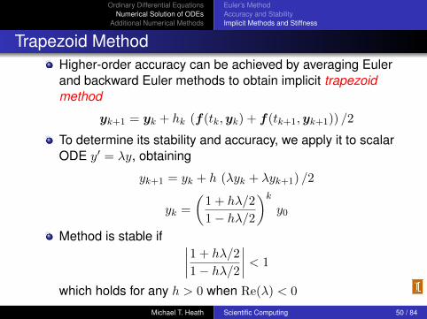
Trapezoid MethodHigher-order accuracy can be achieved by averaging Eulerand backward Euler methods to obtain implicit trapezoidmethod
yk+1 = yk + hk (f(tk,yk) + f(tk+1,yk+1)) /2
To determine its stability and accuracy, we apply it to scalarODE y′ = λy, obtaining
yk+1 = yk + h (λyk + λyk+1) /2
yk =
(1 + hλ/2
1− hλ/2
)ky0
Method is stable if ∣∣∣∣1 + hλ/2
1− hλ/2
∣∣∣∣ < 1
which holds for any h > 0 when Re(λ) < 0
Michael T. Heath Scientific Computing 50 / 84
Ordinary Differential EquationsNumerical Solution of ODEs
Additional Numerical Methods
Euler’s MethodAccuracy and StabilityImplicit Methods and Stiffness
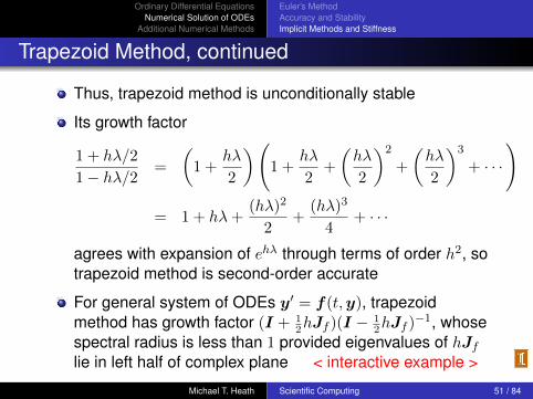
Trapezoid Method, continued
Thus, trapezoid method is unconditionally stable
Its growth factor
1 + hλ/2
1− hλ/2=
(1 +
hλ
2
)(1 +
hλ
2+
(hλ
2
)2
+
(hλ
2
)3
+ · · ·
)
= 1 + hλ+(hλ)2
2+
(hλ)3
4+ · · ·
agrees with expansion of ehλ through terms of order h2, sotrapezoid method is second-order accurate
For general system of ODEs y′ = f(t,y), trapezoidmethod has growth factor (I + 1
2hJf )(I − 12hJf )
−1, whosespectral radius is less than 1 provided eigenvalues of hJflie in left half of complex plane < interactive example >
Michael T. Heath Scientific Computing 51 / 84
Ordinary Differential EquationsNumerical Solution of ODEs
Additional Numerical Methods
Euler’s MethodAccuracy and StabilityImplicit Methods and Stiffness
Implicit Methods, continued
We have now seen two examples of implicit methods thatare unconditionally stable, but not all implicit methods havethis property
Implicit methods generally have larger stability regionsthan explicit methods, but allowable step size is not alwaysunlimited
Implicitness alone is not sufficient to guarantee stability
Michael T. Heath Scientific Computing 52 / 84
Ordinary Differential EquationsNumerical Solution of ODEs
Additional Numerical Methods
Euler’s MethodAccuracy and StabilityImplicit Methods and Stiffness
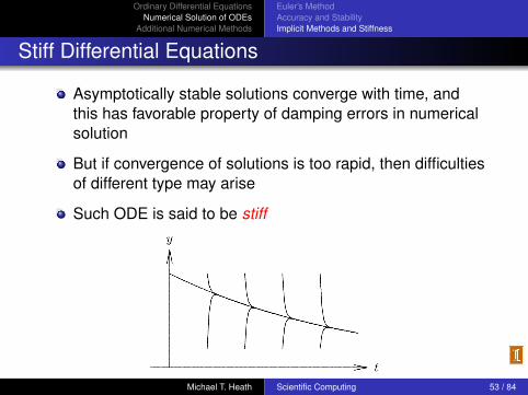
Stiff Differential Equations
Asymptotically stable solutions converge with time, andthis has favorable property of damping errors in numericalsolution
But if convergence of solutions is too rapid, then difficultiesof different type may arise
Such ODE is said to be stiff
Michael T. Heath Scientific Computing 53 / 84
Ordinary Differential EquationsNumerical Solution of ODEs
Additional Numerical Methods
Euler’s MethodAccuracy and StabilityImplicit Methods and Stiffness
Stiff ODEs, continued
Stiff ODE corresponds to physical process whosecomponents have disparate time scales or whose timescale is small compared to interval over which it is studied
System of ODEs y′ = f(t,y) is stiff if eigenvalues of itsJacobian matrix Jf differ greatly in magnitude
There may be eigenvalues with
large negative real parts, corresponding to strongly dampedcomponents of solution, orlarge imaginary parts, corresponding to rapidly oscillatingcomponents of solution
Michael T. Heath Scientific Computing 54 / 84

Ordinary Differential EquationsNumerical Solution of ODEs
Additional Numerical Methods
Euler’s MethodAccuracy and StabilityImplicit Methods and Stiffness
Stiff ODEs, continuedSome numerical methods are inefficient for stiff ODEsbecause rapidly varying component of solution forces verysmall step sizes to maintain stability
Stability restriction depends on rapidly varying componentof solution, but accuracy restriction depends on slowlyvarying component, so step size may be more severelyrestricted by stability than by required accuracy
For example, Euler’s method is extremely inefficient forsolving stiff ODEs because of severe stability limitation onstep size
Backward Euler method is suitable for stiff ODEs becauseof its unconditional stability
Stiff ODEs need not be difficult to solve numerically,provided suitable method is chosen
Michael T. Heath Scientific Computing 55 / 84

Ordinary Differential EquationsNumerical Solution of ODEs
Additional Numerical Methods
Euler’s MethodAccuracy and StabilityImplicit Methods and Stiffness
Example: Stiff ODE
Consider scalar ODE
y′ = −100y + 100t+ 101
with initial condition y(0) = 1
General solution is y(t) = 1 + t+ ce−100t, and particularsolution satisfying initial condition is y(t) = 1 + t(i.e., c = 0)
Since solution is linear, Euler’s method is theoreticallyexact for this problem
However, to illustrate effect of using finite precisionarithmetic, let us perturb initial value slightly
Michael T. Heath Scientific Computing 56 / 84
Ordinary Differential EquationsNumerical Solution of ODEs
Additional Numerical Methods
Euler’s MethodAccuracy and StabilityImplicit Methods and Stiffness
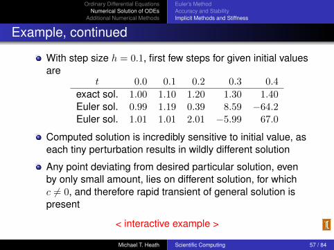
Example, continued
With step size h = 0.1, first few steps for given initial valuesare
t 0.0 0.1 0.2 0.3 0.4
exact sol. 1.00 1.10 1.20 1.30 1.40Euler sol. 0.99 1.19 0.39 8.59 −64.2Euler sol. 1.01 1.01 2.01 −5.99 67.0
Computed solution is incredibly sensitive to initial value, aseach tiny perturbation results in wildly different solution
Any point deviating from desired particular solution, evenby only small amount, lies on different solution, for whichc 6= 0, and therefore rapid transient of general solution ispresent
< interactive example >
Michael T. Heath Scientific Computing 57 / 84

Ordinary Differential EquationsNumerical Solution of ODEs
Additional Numerical Methods
Euler’s MethodAccuracy and StabilityImplicit Methods and Stiffness
Example, continued
Euler’s method bases its projection on derivative at currentpoint, and resulting large value causes numerical solutionto diverge radically from desired solution
Jacobian for this ODE is Jf = −100, so stability conditionfor Euler’s method requires step size h < 0.02, which weare violating
Michael T. Heath Scientific Computing 58 / 84
Ordinary Differential EquationsNumerical Solution of ODEs
Additional Numerical Methods
Euler’s MethodAccuracy and StabilityImplicit Methods and Stiffness
Example, continued
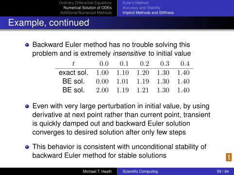
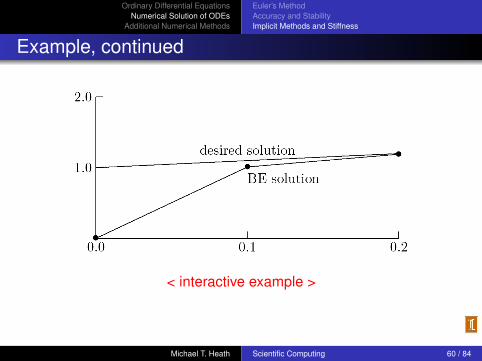
Backward Euler method has no trouble solving thisproblem and is extremely insensitive to initial value
t 0.0 0.1 0.2 0.3 0.4
exact sol. 1.00 1.10 1.20 1.30 1.40BE sol. 0.00 1.01 1.19 1.30 1.40BE sol. 2.00 1.19 1.21 1.30 1.40
Even with very large perturbation in initial value, by usingderivative at next point rather than current point, transientis quickly damped out and backward Euler solutionconverges to desired solution after only few steps
This behavior is consistent with unconditional stability ofbackward Euler method for stable solutions
Michael T. Heath Scientific Computing 59 / 84
Ordinary Differential EquationsNumerical Solution of ODEs
Additional Numerical Methods
Euler’s MethodAccuracy and StabilityImplicit Methods and Stiffness
Example, continued
< interactive example >
Michael T. Heath Scientific Computing 60 / 84
Ordinary Differential EquationsNumerical Solution of ODEs
Additional Numerical Methods
Single-Step MethodsExtrapolation MethodsMultistep Methods
Numerical Methods for ODEs
There are many different methods for solving ODEs, most ofwhich are of one of following types
Taylor series
Runge-Kutta
Extrapolation
Multistep
Multivalue
We briefly consider each of these types of methods
Michael T. Heath Scientific Computing 61 / 84
Ordinary Differential EquationsNumerical Solution of ODEs
Additional Numerical Methods
Single-Step MethodsExtrapolation MethodsMultistep Methods
Taylor Series Methods
Euler’s method can be derived from Taylor seriesexpansion
By retaining more terms in Taylor series, we can generatehigher-order single-step methods
For example, retaining one additional term in Taylor series
y(t+ h) = y(t) + hy′(t) +h2
2y′′(t) +
h3
6y′′′(t) + · · ·
gives second-order method
yk+1 = yk + hk y′k +
h2k2y′′k
Michael T. Heath Scientific Computing 62 / 84

Ordinary Differential EquationsNumerical Solution of ODEs
Additional Numerical Methods
Single-Step MethodsExtrapolation MethodsMultistep Methods
Taylor Series Methods, continued
This approach requires computation of higher derivativesof y, which can be obtained by differentiating y′ = f(t,y)using chain rule, e.g.,
y′′ = ft(t,y) + fy(t,y)y′
= ft(t,y) + fy(t,y)f(t,y)
where subscripts indicate partial derivatives with respect togiven variable
As order increases, expressions for derivatives rapidlybecome too complicated to be practical to compute, soTaylor series methods of higher order have not often beenused in practice
< interactive example >
Michael T. Heath Scientific Computing 63 / 84

Ordinary Differential EquationsNumerical Solution of ODEs
Additional Numerical Methods
Single-Step MethodsExtrapolation MethodsMultistep Methods
Runge-Kutta Methods
Runge-Kutta methods are single-step methods similar inmotivation to Taylor series methods, but they do not requirecomputation of higher derivatives
Instead, Runge-Kutta methods simulate effect of higherderivatives by evaluating f several times between tk andtk+1
Simplest example is second-order Heun’s method
yk+1 = yk +hk2
(k1 + k2)
where
k1 = f(tk,yk)
k2 = f(tk + hk,yk + hkk1)
Michael T. Heath Scientific Computing 64 / 84

Ordinary Differential EquationsNumerical Solution of ODEs
Additional Numerical Methods
Single-Step MethodsExtrapolation MethodsMultistep Methods
Runge-Kutta Methods, continued
Heun’s method is analogous to implicit trapezoid method,but remains explicit by using Euler prediction yk + hkk1instead of y(tk+1) in evaluating f at tk+1
Best known Runge-Kutta method is classical fourth-orderscheme
yk+1 = yk +hk6
(k1 + 2k2 + 2k3 + k4)
where
k1 = f(tk,yk)
k2 = f(tk + hk/2,yk + (hk/2)k1)
k3 = f(tk + hk/2,yk + (hk/2)k2)
k4 = f(tk + hk,yk + hkk3)
< interactive example >Michael T. Heath Scientific Computing 65 / 84

Ordinary Differential EquationsNumerical Solution of ODEs
Additional Numerical Methods
Single-Step MethodsExtrapolation MethodsMultistep Methods
Runge-Kutta Methods, continued
To proceed to time tk+1, Runge-Kutta methods require nohistory of solution prior to time tk, which makes themself-starting at beginning of integration, and also makes iteasy to change step size during integration
These facts also make Runge-Kutta methods relativelyeasy to program, which accounts in part for their popularity
Unfortunately, classical Runge-Kutta methods provide noerror estimate on which to base choice of step size
Michael T. Heath Scientific Computing 66 / 84

Ordinary Differential EquationsNumerical Solution of ODEs
Additional Numerical Methods
Single-Step MethodsExtrapolation MethodsMultistep Methods
Runge-Kutta Methods, continued
Fehlberg devised embedded Runge-Kutta method thatuses six function evaluations per step to produce bothfifth-order and fourth-order estimates of solution, whosedifference provides estimate for local error
Another embedded Runge-Kutta method is due toDormand and Prince
This approach has led to automatic Runge-Kutta solversthat are effective for many problems, but which arerelatively inefficient for stiff problems or when very highaccuracy is required
It is possible, however, to define implicit Runge-Kuttamethods with superior stability properties that are suitablefor solving stiff ODEs
Michael T. Heath Scientific Computing 67 / 84
Ordinary Differential EquationsNumerical Solution of ODEs
Additional Numerical Methods
Single-Step MethodsExtrapolation MethodsMultistep Methods
Extrapolation Methods
Extrapolation methods are based on use of single-stepmethod to integrate ODE over given interval tk ≤ t ≤ tk+1
using several different step sizes hi, and yielding resultsdenoted by Y (hi)
This gives discrete approximation to function Y (h), whereY (0) = y(tk+1)
Interpolating polynomial or rational function Y (h) is fit tothese data, and Y (0) is then taken as approximation toY (0)
Extrapolation methods are capable of achieving very highaccuracy, but they are much less efficient and less flexiblethan other methods for ODEs, so they are not often usedunless extremely high accuracy is required and cost is notsignificant factor < interactive example >
Michael T. Heath Scientific Computing 68 / 84
Ordinary Differential EquationsNumerical Solution of ODEs
Additional Numerical Methods
Single-Step MethodsExtrapolation MethodsMultistep Methods
Multistep Methods
Multistep methods use information at more than oneprevious point to estimate solution at next point
Linear multistep methods have form
yk+1 =
m∑i=1
αiyk+1−i + h
m∑i=0
βif(tk+1−i,yk+1−i)
Parameters αi and βi are determined by polynomialinterpolation
If β0 = 0, method is explicit, but if β0 6= 0, method is implicit
Implicit methods are usually more accurate and stable thanexplicit methods, but require starting guess for yk+1
Michael T. Heath Scientific Computing 69 / 84
Ordinary Differential EquationsNumerical Solution of ODEs
Additional Numerical Methods
Single-Step MethodsExtrapolation MethodsMultistep Methods
Multistep Methods, continued
Starting guess is conveniently supplied by explicit method,so the two are used as predictor-corrector pair
One could use corrector repeatedly (i.e., fixed-pointiteration) until some convergence tolerance is met, but itmay not be worth expense
So fixed number of corrector steps, often only one, may beused instead, giving PECE scheme (predict, evaluate,correct, evaluate)
Although it has no effect on value of yk+1, secondevaluation of f in PECE scheme yields improved value ofy′k+1 for future use
Michael T. Heath Scientific Computing 70 / 84
Ordinary Differential EquationsNumerical Solution of ODEs
Additional Numerical Methods
Single-Step MethodsExtrapolation MethodsMultistep Methods
Multistep Methods, continued
Alternatively, nonlinear equation for yk+1 given by implicitmultistep method can be solved by Newton’s method orsimilar method, again with starting guess supplied bysolution at previous step or by explicit multistep method
Newton’s method or close variant of it is essential whenusing an implicit multistep method designed for stiff ODEs,as fixed-point iteration fails to converge for reasonable stepsizes
< interactive example >
Michael T. Heath Scientific Computing 71 / 84

Ordinary Differential EquationsNumerical Solution of ODEs
Additional Numerical Methods
Single-Step MethodsExtrapolation MethodsMultistep Methods
Examples: Multistep Methods
Simplest second-order accurate explicit two-step method is
yk+1 = yk +h
2(3y′k − y′k−1)
Simplest second-order accurate implicit method istrapezoid method
yk+1 = yk +h
2(y′k+1 + y
′k)
One of most popular pairs of multistep methods is explicitfourth-order Adams-Bashforth predictor
yk+1 = yk +h
24(55y′k − 59y′k−1 + 37y′k−2 − 9y′k−3)
and implicit fourth-order Adams-Moulton corrector
yk+1 = yk +h
24(9y′k+1 + 19y′k − 5y′k−1 + y
′k−2)
Michael T. Heath Scientific Computing 72 / 84

Ordinary Differential EquationsNumerical Solution of ODEs
Additional Numerical Methods
Single-Step MethodsExtrapolation MethodsMultistep Methods
Examples: Multistep Methods
Backward differentiation formulas form another importantfamily of implicit multistep methods
BDF methods, typified by popular formula
yk+1 =1
11(18yk − 9yk−1 + 2yk−2) +
6h
11y′k+1
are effective for solving stiff ODEs
< interactive example >
Michael T. Heath Scientific Computing 73 / 84
Ordinary Differential EquationsNumerical Solution of ODEs
Additional Numerical Methods
Single-Step MethodsExtrapolation MethodsMultistep Methods
Multistep Adams Methods
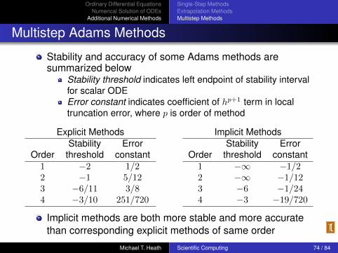
Stability and accuracy of some Adams methods aresummarized below
Stability threshold indicates left endpoint of stability intervalfor scalar ODEError constant indicates coefficient of hp+1 term in localtruncation error, where p is order of method
Explicit MethodsStability Error
Order threshold constant1 −2 1/22 −1 5/123 −6/11 3/84 −3/10 251/720
Implicit MethodsStability Error
Order threshold constant1 −∞ −1/22 −∞ −1/123 −6 −1/244 −3 −19/720
Implicit methods are both more stable and more accuratethan corresponding explicit methods of same order
Michael T. Heath Scientific Computing 74 / 84
Ordinary Differential EquationsNumerical Solution of ODEs
Additional Numerical Methods
Single-Step MethodsExtrapolation MethodsMultistep Methods
Properties of Multistep Methods
They are not self-starting, since several previous values ofyk are needed initially
Changing step size is complicated, since interpolationformulas are most conveniently based on equally spacedintervals for several consecutive points
Good local error estimate can be determined fromdifference between predictor and corrector
They are relatively complicated to program
Being based on interpolation, they can efficiently providesolution values at output points other than integrationpoints
Michael T. Heath Scientific Computing 75 / 84

Ordinary Differential EquationsNumerical Solution of ODEs
Additional Numerical Methods
Single-Step MethodsExtrapolation MethodsMultistep Methods
Properties of Multistep, continued
Implicit methods have much greater region of stability thanexplicit methods, but must be iterated to convergence toenjoy this benefit fully
PECE scheme is actually explicit, though in a somewhatcomplicated way
Although implicit methods are more stable than explicitmethods, they are still not necessarily unconditionallystable
No multistep method of greater than second order isunconditionally stable, even if it is implicit
Properly designed implicit multistep method can be veryeffective for solving stiff ODEs
Michael T. Heath Scientific Computing 76 / 84
Ordinary Differential EquationsNumerical Solution of ODEs
Additional Numerical Methods
Single-Step MethodsExtrapolation MethodsMultistep Methods
Multivalue Methods
With multistep methods it is difficult to change step size,since past history of solution is most easily maintained atequally spaced intervals
Like multistep methods, multivalue methods are alsobased on polynomial interpolation, but avoid someimplementation difficulties associated with multistepmethods
One key idea motivating multivalue methods is observationthat interpolating polynomial itself can be evaluated at anypoint, not just at equally spaced intervals
Equal spacing associated with multistep methods is artifactof representation as linear combination of successivesolution and derivative values with fixed weights
Michael T. Heath Scientific Computing 77 / 84
Ordinary Differential EquationsNumerical Solution of ODEs
Additional Numerical Methods
Single-Step MethodsExtrapolation MethodsMultistep Methods
Multivalue Methods, continued
Another key idea in implementing multivalue methods isrepresenting interpolating polynomial so that parametersare values of solution and its derivatives at tk
This approach is analogous to using Taylor, rather thanLagrange, representation of polynomial
Solution is advanced in time by simple transformation ofrepresentation from one point to next, and it is easy tochange step size
Multivalue methods are mathematically equivalent tomultistep methods but are more convenient and flexible toimplement, so most modern software implementations arebased on them
Michael T. Heath Scientific Computing 78 / 84
Ordinary Differential EquationsNumerical Solution of ODEs
Additional Numerical Methods
Single-Step MethodsExtrapolation MethodsMultistep Methods
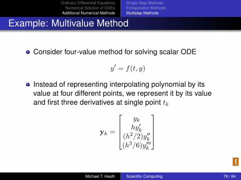
Example: Multivalue Method
Consider four-value method for solving scalar ODE
y′ = f(t, y)
Instead of representing interpolating polynomial by itsvalue at four different points, we represent it by its valueand first three derivatives at single point tk
yk =
ykhy′k
(h2/2)y′′k(h3/6)y′′′k
Michael T. Heath Scientific Computing 79 / 84
Ordinary Differential EquationsNumerical Solution of ODEs
Additional Numerical Methods
Single-Step MethodsExtrapolation MethodsMultistep Methods
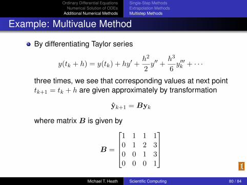
Example: Multivalue Method
By differentiating Taylor series
y(tk + h) = y(tk) + hy′ +h2
2y′′ +
h3
6y′′′k + · · ·
three times, we see that corresponding values at next pointtk+1 = tk + h are given approximately by transformation
yk+1 = Byk
where matrix B is given by
B =
1 1 1 10 1 2 30 0 1 30 0 0 1
Michael T. Heath Scientific Computing 80 / 84
Ordinary Differential EquationsNumerical Solution of ODEs
Additional Numerical Methods
Single-Step MethodsExtrapolation MethodsMultistep Methods
Example: Multivalue Method
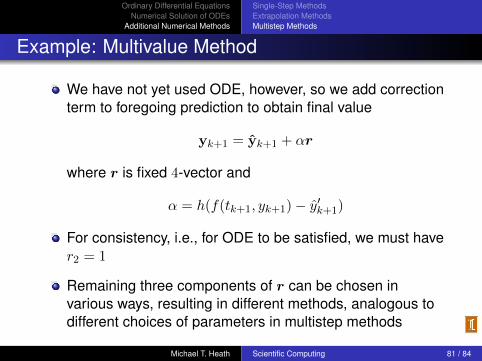
We have not yet used ODE, however, so we add correctionterm to foregoing prediction to obtain final value
yk+1 = yk+1 + αr
where r is fixed 4-vector and
α = h(f(tk+1, yk+1)− y′k+1)
For consistency, i.e., for ODE to be satisfied, we must haver2 = 1
Remaining three components of r can be chosen invarious ways, resulting in different methods, analogous todifferent choices of parameters in multistep methods
Michael T. Heath Scientific Computing 81 / 84
Ordinary Differential EquationsNumerical Solution of ODEs
Additional Numerical Methods
Single-Step MethodsExtrapolation MethodsMultistep Methods
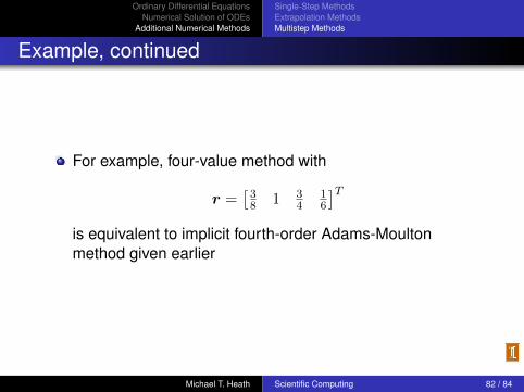
Example, continued
For example, four-value method with
r =[38 1 3
416
]Tis equivalent to implicit fourth-order Adams-Moultonmethod given earlier
Michael T. Heath Scientific Computing 82 / 84

Ordinary Differential EquationsNumerical Solution of ODEs
Additional Numerical Methods
Single-Step MethodsExtrapolation MethodsMultistep Methods
Multivalue Methods, continued
It is easy to change step size with multivalue methods: weneed merely rescale components of yk to reflect new stepsize
It is also easy to change order of method simply bychanging components of r
These two capabilities, combined with sophisticated testsand strategies for deciding when to change order and stepsize, have led to development of powerful and efficientsoftware packages for solving ODEs based onvariable-order/variable-step methods
Michael T. Heath Scientific Computing 83 / 84
Ordinary Differential EquationsNumerical Solution of ODEs
Additional Numerical Methods
Single-Step MethodsExtrapolation MethodsMultistep Methods
Variable-Order/Variable-Step Solvers
Such routines are analogous to adaptive quadratureroutines: they automatically adapt to given problem,varying order and step size of integration method asnecessary to meet user-supplied error tolerance efficiently
Such routines often have options for solving either stiff ornonstiff problems, and some even detect stiffnessautomatically and select appropriate method accordingly
Ability to change order easily also obviates need forspecial starting procedures: one can simply start withfirst-order method, which requires no additional startingvalues, and let automatic order/step size selectionprocedure increase order as needed for required accuracy
Michael T. Heath Scientific Computing 84 / 84
Related Documents