SCHRIFTENREIHE SCHIFFBAU - TUHH · SCHRIFTENREIHE SCHIFFBAU Anja Kömpe Implementation and Validation of a Wave Cut ... The Holtrop-Mennen method is the most common empirical technique.

SCHRIFTENREIHE SCHIFFBAU

Anja Kömpe

Implementation and Validation of a Wave Cut Analysis Method for the Wave Resistance Prediction from Potential Flow

A-66 | Oktober 2014

Hamburg University of TechnologyInstitute of Ship Design and Ship Safety

Master’s Thesis

Implementation and Validation of

a Wave Cut Analysis Method

for the Wave Resistance Prediction

from Potential Flow

Anja Kompe

First Examiner: Prof. Dr.-Ing. Stefan Kruger

Second Examiner: Prof. Dr.-Ing. Moustafa Abdel-Maksoud

Supervisor: Dipl.-Ing. Johannes Will

Date: 24. Oktober 2014

Redigierte Version vom 16.02.2015

Declaration of Authorship

I hereby declare and confirm that this thesis and the work presented in it havebeen generated by me as the result of my own original research and that I havenot made use of any other sources than those stated in here.

Place, Date Signature

Contents

List of Figures III

List of Tables IV

Nomenclature VII

1 Introduction 11.1 Resistance Prediction . . . . . . . . . . . . . . . . . . . . . . . . . . 11.2 Task . . . . . . . . . . . . . . . . . . . . . . . . . . . . . . . . . . . 2

2 Theory 32.1 Resistance . . . . . . . . . . . . . . . . . . . . . . . . . . . . . . . . 32.2 Momentum Considerations . . . . . . . . . . . . . . . . . . . . . . . 52.3 Potential Flow . . . . . . . . . . . . . . . . . . . . . . . . . . . . . . 8

3 Review of Previous Work 103.1 Havelock . . . . . . . . . . . . . . . . . . . . . . . . . . . . . . . . . 123.2 Transverse wave cut analysis . . . . . . . . . . . . . . . . . . . . . . 143.3 Longitudinal wave cut analysis . . . . . . . . . . . . . . . . . . . . . 163.4 XY Method . . . . . . . . . . . . . . . . . . . . . . . . . . . . . . . 193.5 Soding . . . . . . . . . . . . . . . . . . . . . . . . . . . . . . . . . . 19

4 Implementation of a Wave Cut Analysis 234.1 Outline of Current Work . . . . . . . . . . . . . . . . . . . . . . . . 234.2 Wave Heights Computation by Newton’s Method . . . . . . . . . . 254.3 Discretization and Position of Transverse Wave Cuts . . . . . . . . 284.4 Fourier Coefficients Calculation and Free Wave Spectrum . . . . . . 304.5 Wave Resistance Computation . . . . . . . . . . . . . . . . . . . . . 334.6 Alternative Approaches . . . . . . . . . . . . . . . . . . . . . . . . . 35

4.6.1 Direct evaluation of the velocity potential . . . . . . . . . . 354.6.2 Longitudinal wave cut method . . . . . . . . . . . . . . . . . 36

5 Validation 375.1 Case 1: Wigley Hull . . . . . . . . . . . . . . . . . . . . . . . . . . 37

5.1.1 Wigley Hull . . . . . . . . . . . . . . . . . . . . . . . . . . . 375.1.2 Wave Field and Floating Position . . . . . . . . . . . . . . . 385.1.3 Wave Resistance . . . . . . . . . . . . . . . . . . . . . . . . 40

5.2 Case 2: RoRo ferry . . . . . . . . . . . . . . . . . . . . . . . . . . . 455.2.1 RoRo ferry . . . . . . . . . . . . . . . . . . . . . . . . . . . 455.2.2 Wave Resistance . . . . . . . . . . . . . . . . . . . . . . . . 465.2.3 Form Factor by Prohaska’s Method . . . . . . . . . . . . . . 50

I

6 Summary and Conclusion 52

References 57

A Wave Resistances of Wigley Hull from Literature 59

B Wave Resistance Results of Wigley Hull 63

C Wave Resistance Results of RoRo ferry 64

II

List of Figures

2.1 Energy balance . . . . . . . . . . . . . . . . . . . . . . . . . . . . . 52.2 Control surfaces of rectangular control volume . . . . . . . . . . . . 53.1 Classification of wave cut analysis methods . . . . . . . . . . . . . . 103.2 XY method geometry . . . . . . . . . . . . . . . . . . . . . . . . . . 194.1 Newton’s method . . . . . . . . . . . . . . . . . . . . . . . . . . . . 254.2 Iteration of water surface by bisection method . . . . . . . . . . . . 264.3 Iteration of water surface by Newton’s method . . . . . . . . . . . . 274.4 Wave field example according to Soding . . . . . . . . . . . . . . . . 284.5 Transverse wave cuts and control area. . . . . . . . . . . . . . . . . 294.6 Free wave spectrum for Fn = 0.188 and Fn = 0.325 . . . . . . . . . . 325.1 Wigley hull: Hull grid . . . . . . . . . . . . . . . . . . . . . . . . . 375.2 Wigely hull: Wave elevation along hull . . . . . . . . . . . . . . . . 385.3 Wigley hull: running trim . . . . . . . . . . . . . . . . . . . . . . . 395.4 Wigley hull: sinkage . . . . . . . . . . . . . . . . . . . . . . . . . . 395.5 Wigley hull: Computed wave resistance coefficients . . . . . . . . . 415.6 Wigley hull, free model: Computed wave resistance coefficients . . . 415.7 Wigley hull, free model: Comparison with wave resistance measure-

ments . . . . . . . . . . . . . . . . . . . . . . . . . . . . . . . . . . 425.8 Wigley hull, fixed model: Comparison with wave resistance mea-

surements . . . . . . . . . . . . . . . . . . . . . . . . . . . . . . . . 435.9 Wigley hull, free model: Comparison with wave resistance calculations 445.10 Wigley hull, fixed model: Comparison with wave resistance calcu-

lations . . . . . . . . . . . . . . . . . . . . . . . . . . . . . . . . . . 445.11 RoRo ferry: Coarse hull grid . . . . . . . . . . . . . . . . . . . . . . 455.12 RoRo ferry: Fine hull grid . . . . . . . . . . . . . . . . . . . . . . . 465.13 RoRo ferry: Wave resistance coefficient, fine resolution of hull and

free surface . . . . . . . . . . . . . . . . . . . . . . . . . . . . . . . 475.14 RoRo ferry: Wave resistance coefficient, coarse resolution of hull

and free surface . . . . . . . . . . . . . . . . . . . . . . . . . . . . . 485.15 RoRo ferry: Comparison of fine and coarse resolution of hull and

free surface . . . . . . . . . . . . . . . . . . . . . . . . . . . . . . . 495.16 RoRo ferry: Comparison of fine and coarse hull grid, fine surface grid 495.17 RoRo ferry: Form factor by Prohaska’s method . . . . . . . . . . . 505.18 RoRo ferry: Wave resistance coefficients with form factor . . . . . . 51A.1 Wigley hull, free model: Measured wave resistance data . . . . . . . 59A.2 Wigley hull, fixed model: Measured wave resistance data . . . . . . 61A.3 Wigley hull, free model: Calculated wave resistance data . . . . . . 61A.4 Wigley hull, free model: Calculated wave resistance data . . . . . . 62

III

List of Tables

3.1 Review of wave cut analysis . . . . . . . . . . . . . . . . . . . . . . 115.1 Overview of wave resistance calculation methods . . . . . . . . . . . 405.2 RoRo ferry: Main dimensions . . . . . . . . . . . . . . . . . . . . . 45A.1 Wigley hull, free model: Experimental Data WPHGD . . . . . . . . 60A.2 Wigley hull, free model: Calculation Zou . . . . . . . . . . . . . . . 62B.1 Wigley hull, free model: Wave resistance coefficients . . . . . . . . . 63B.2 Wigley hull, fixed model: Wave resistance coefficients . . . . . . . . 64C.1 RoRo ferry: Wave resistance coefficients from model test . . . . . . 64C.2 RoRo ferry: Wave resistance coefficients, fine resolution of hull and

free surface . . . . . . . . . . . . . . . . . . . . . . . . . . . . . . . 65C.3 RoRo ferry: Wave resistance coefficients, coarse resolution of hull

and free surface . . . . . . . . . . . . . . . . . . . . . . . . . . . . . 65C.4 RoRo ferry: Wave resistance coefficients, coarse hull grid, fine sur-

face grid . . . . . . . . . . . . . . . . . . . . . . . . . . . . . . . . . 65

IV

Nomenclature

Latin Letters

B bottomFS free surfaceH hull

LWC longitudinal wave cutPS portside

RANS Reynolds-Averaged Navier-StokesRINA Royal Institution of Naval Architects

S surface [m2]SB starboard

TWC transverse wave cutV volume [m3]

WPHGD Wigley parabolic hull group discussion

1+k form factor [–]a wave amplitude [m]an Fourier coefficient [m]Aw wetted surface [m2]

A(α) free wave spectrum [m]a(α) cosinus component of free wave spectrum [m]

B breadth of controll volume [m]B ship’s breadth [m]bn Fourier coefficient [m]

b(α) sinus component of free wave spectrum [m]c phase speed of waves [m s−1]

C′(k′x) weighted Fourier transform of LWC [–]c1, c2, c3 constants for truncation correction [–]

CB blockcoefficient [–]CF0 friction coefficient according to ITTC-57

correlation line[–]

CF viscous resistance coefficient [–]cgr group velocity of waves [m s−1]CR residuary resistance coefficient [–]CT total resistance coefficient [–]CW wave resistance coefficient [–]

C(k′x) Fourier transform of LWC [–]D draught [m]E energy [N m] [kg m2 s−2]e specific energy [N/m]

V

E energy flow [N m/s] [kg m2 s−3]F force [N] [kg m s−2]~f = (0, 0, g) volume force per unit vol-

ume[m s−2]

f(α) function of wave amplitudes [m]Fn Froude number [–]g acceleration due to gravity [m s−2]h water depht [m]k wavenumber [m−1]k0 = g/U2 basic wavenumber [m]k1 direction coefficient of Prohaska’s

method[–]

kx = k cosα component of wavenumber inx-direction

[m−1]

ky = k sinα component of wavenumber iny-direction

[m−1]

L ship’s length [m]Lao length over all [m]Lpp length between perpendiculars [m]N number of Fourier coefficients [–]~n normal vector [m]P power [W] [kg m2 s−3]p pressure [N/m2] [kg m−1 s−2]Q momentum [N s] [kg m s−1]R resistance [kN] [kg m s−2]

RT total resistance [kN] [kg m s−2]RW wave resistance [kN] [kg m s−2]Rn Reynolds number [–]

S′(k′x) weighted Fourier transform of LWC [–]S(k′x) Fourier transform of LWC [–]

t time [s]U ship’s speed [kn] [m s−1]u flow velocity in x-direction [m s−1]~u = (u, v, w) flow velocity [m s−1]v flow velocity in y-direction [m s−1]

Vn velocity of boundary surface in normal di-rection

[m s−1]

w flow velocity in z-direction [m s−1]X cylinder force in x-direction [N] [kg m s−2]x coordinate in ship’s motion direction [m]x′ abbrevation for x - Ut [m]xE x-position of truncation point [m]

VI

Y cylinder force in y-direction [N] [kg m s−2]y horizontal coordinate positive to portside [m]z vertical coordinate positive upwards [m]

Greek Letters

α propagation angle [◦] [rad]βn abbrevation for knxx+ knyy [–]η geometry of ship hull [m]λ wavelength [m]ω circular frequency [s−1]Φ velocity potential [m2 s−1]Φx derivation of velocity potential with re-

spect to x[m s−1]

Φy derivation of velocity potential with re-spect to y

[m s−1]

Φz derivation of velocity potential with re-spect to z

[m s−1]

ρ density of water [kg m−3]τ shear stress [N/m2] [kg m−1 s−2]

ζ(x,y) wave elevation [m]

| ζ | wave amplitude [m]

Superscripts

′ non-dimensional quantity

Subscripts

k grid point indexkin kineticn coefficient indexn normal direction

pot potential

VII

1 Introduction

A strict specification in the contract between a new ship owner and the shipyardis the so-called contract speed. This is a defined speed the ship has to attain incompliance with sea and engine margines. The required engine power depends,besides minor factors like propulsive efficiency and losses in the power train, onthe resistance of the ship. Thus the resistance is an important parameter in shipdesign.

However, ship design is an iterative process. The requiered break power of themain engine and subsequently the fuel storage capacity depend mainly on theresistance. Yet, saving the weight of for example one cylinder of the main engineprovides optimization potential of the hull form through displacement reduction.Thus the calm water resistance prediction already at an early stage in the project isnecessary to design an efficient ship. During optimization process a fast evaluationof hull form changes is needed. With an increasing level of details the accuracy ofprediction has to rise.

1.1 Resistance Prediction

Investigation of resistance and resistance prediction started with model experi-ments. In 1868 Froude proposed his law of comparison to scale model results tofull scale. In principle his method is still in use for the evaluation of model tests.

Besides, two other widely indempendent procedures for calm water resistanceprediction are available: Firstly empirical formulae and secondly computationalmethods, divided into boundary elements methods, that solve Laplace’s equation,and volume elements methods.

The Holtrop-Mennen method is the most common empirical technique. Com-putational methods started with linearized inviscous boundary elements methods.A pioneering work on the boundary value problem has been made by Michell in1898 [1], [2]. His formula, known as Michell integral, solves the Michell-Kelvinproblem (linearized body and linearized free surface condition). With progressof computer technology, more advanced potential flow methods became possible.Starting from the Neumann-Kelvin problem (hull boundary condition on hull sur-face, linearized free surface condition), nowadays potential method programs solvethe fully non-linear Neumann-Stokes problem.

Typical volume element methods, so-called RANS methods, solve the Reynolds-Averaged Navier-Stokes equations. They take viscosity into account.

Potential methods determine the resistance from pressure integration over thewetted hull surface. RANS calculations include as well the force from integratedshear stresses. However, the common pressure integration method is sensitive tothe discretization of the hull. Local irregularities of the computational mesh canhave major impacts on the computed resistance. Thus the reliability is considered

1

poor.Alternatively, the wave resistance can be determined by so-called wave cut anal-

ysis. Based on energy considerations, the wave resistance is computed from thewave pattern of the ship. Wave pattern are less sensitive to irregularities of thediscretization. Therefore wave cut analysis is expected to be more robust than thepressure integration [3], [4]. Wave pattern can be derived from a computationalmethod or be measured during a model test.

A final determination of the resistance is performed during the sea trial for thedelivery of the ship. As then the ship is already build, this method is only in caseof series of ships suitable for resistance prediction.

Regarding the previously presented methods, these vary in accuracy of the pre-diction and requiered effort. Model tests are well established. Due to empiricalknowledge of the towing tank institutes, the accuracy is high, especially for wellknown conventional types of vessels. However, the tests are expensive and time-consuming.

Empirical methods are simple and fast. They can be performed already whenonly main characteristics of the ship are known. In return they are quite unprecise.Due to the fact, that empirical methods are developed using typical hull forms,they are inappropriate for innovative designs.

Potential methods are quicker than RANS methods. However, viscous effectshave to be estimated. Since there is much more hull form optimization potentialregarding the wave than the frictional resistance, potential methods are suitablefor comparative hull form evaluation. RANS methods are expected to be moreaccurate, as the calculation includes viscous effects. Therefore they are much moretime-consuming in preparation and execution than potential solvers. Since onlythe primary wave system is described correctly, RANS methods are inappropriatefor evaluation of interferences.

1.2 Task

As described above, pressure integration is sensitive to the hull from discretization.Wave cut analysis promises a conceptual solution, since the resistance is calculatedfrom given wave pattern without explicit reference to the cause of the wave making.

The goal of this thesis is the implementation and validation of a wave cut anal-ysis. Thus first a literature research has to be carried out. A review presentsrelevant approaches of wave cut analysis. Then a reliable technique should beimplemented.

The correct implementation is validated on the basis of the Wigley hull testcase. This simple ship-like test case allows an investigation of impacts of imple-mentational aspects. Calculated results can be validated by values from literature.Finally, the wave cut analysis is used for resistance prediction of a RoRo ferry.

2

2 Theory

In the following chapter, first some observations of the resistance of a ship aremade. Then a general formula for wave resistance is developed from momentumconsiderations. Finally, potential theory is presented, as a basis of wave flowmodels and wave field calculation.

2.1 Resistance

The resistance results from shear and normal stresses on the hull surface caused bythe water flow. In addition, there are forces on the superstructures of the ship fromairflow. Excluding additional resistances for example due to sea state or wind, theresistance consists of the following components:

Rtotal = Rwaves +Rviscous +Rappendages +Rair (2.1)

The main components are the wave and the viscous resistance. Each of themcan be split up further. The appendages resistance is mainly of viscous origin.However, it is treated separately. The smaller Reynolds numbers of the appendagesin comparison with that of the hull require an extra scaling. In the following,appendages and air resistance are not considered further.There are alternative decompositions of resistance like for example into normalforces (pressure) and tangential forces (friction) :

RT =

∮pnxdS +

∮τnxdS (2.2)

However, the decomposition into wave and viscous resistance is most directly re-lated with separate physical phenomena. Considering model tests, equal Reynoldsnumbers at both scales are required for correct effects of viscosity. For gravityeffects on the free surface (wave making) equality of Froude numbers is needed.For scaling non-dimensional force coefficients are introduced:

CT =1

12ρU2

∮p~nxdS∮dS

=RT

12ρU2Aw

(2.3)

Actually, the wave resistance (moment of 1. order) is divided by the true wettedsurface Aw =

∮dS (moment of 0. order). Depending on the velocity of the ship, the

true wetted surface varies, considering waves and changes in trim. However, thissurface is unknown during model tests. Thus, coefficients from model experimentsare derived by using the wetted surface of the initial floating position at zero speed.For reasons of comparability, the initial wetted surface is used in this work as wellfor the results from computational methods.

According to Froude’s hypothesis, model tests are carried out at equal Froudenumbers. Then a residuary resistance is calculated by substracting an estimated

3

viscous resistance from the measured total resistance. The most important partof this residuary resistance is the wave resistance [5]. However, the wave andthe residuary resistance are not quite equal, due to insufficiencies of the viscousresistance estimation.

The viscous resistance has to be estimated for the model and the full scaleship. The coefficients, depending of the corresponding Reynolds numbers, arecalculated according to ITTC-57 recommendations or ITTC-78 recommendations[6]. The ITTC-57 correlation line determines the viscous resistance coefficient fromflat plate friction including some effect of the 3D shape of the ship:

CF0 =0.075

(log Rn− 2)2(2.4)

The ITTC-78 procedure introduces a form factor

1 + k =CFCF0

(2.5)

to consider form effects on the friction more precisely and individually for eachship. Despite the interaction between the wave making of a ship and the viscousflow around it, the resistance coefficient is approximated by:

CT (Fn,Rn) ≈ CR(Fn) + CF (Rn) (2.6)

Regarding presented computational techniques, the viscous resistance can betaken into account only by RANS methods. The calculated resistance from po-tential methods represents only the wave resistance. However, the determinationaccording to ITTC-57 correlation line is well established and regarding hull formoptimization, the wave resistance is more relevant than viscous effects. Thus, inthe following, the prediction of wave resistance is examined.

The wave resistance of a ship is defined as the flow of energy into the ships wavepattern, divided by the ship speed [7].

RW =flow of energy (ship → wave pattern)

ship speed(2.7)

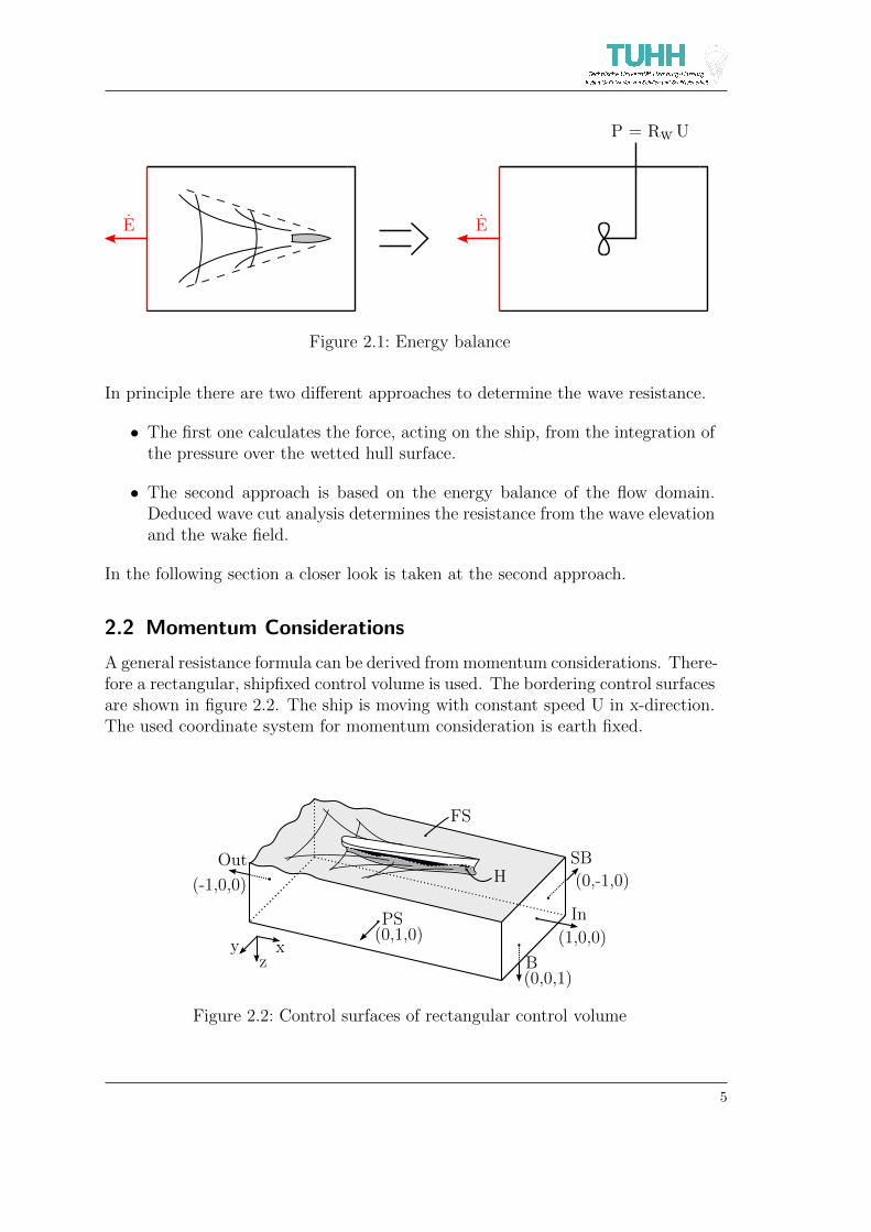
Figure 2.1 illustrates this definition. All boundary surfaces, except the one behindthe ship (red), are assumed to be so far away, that the water is undisturbed. Thusthe balance of energy requires, that the energy flow over the rear boundary surfaceequals the power, which is put into the system. On the right side of the figure theenergy supply is represented symbolically. In case of the moving ship the towingpower RW U constitutes this energy flow.

4

E E

P = Rw U

Figure 2.1: Energy balance

In principle there are two different approaches to determine the wave resistance.

• The first one calculates the force, acting on the ship, from the integration ofthe pressure over the wetted hull surface.

• The second approach is based on the energy balance of the flow domain.Deduced wave cut analysis determines the resistance from the wave elevationand the wake field.

In the following section a closer look is taken at the second approach.

2.2 Momentum Considerations

A general resistance formula can be derived from momentum considerations. There-fore a rectangular, shipfixed control volume is used. The bordering control surfacesare shown in figure 2.2. The ship is moving with constant speed U in x-direction.The used coordinate system for momentum consideration is earth fixed.

FS

PS

B

H

In

Out

(0,1,0)

(0,-1,0)

(0,0,1)

(1,0,0)

(-1,0,0)

xyz

SB

Figure 2.2: Control surfaces of rectangular control volume

5

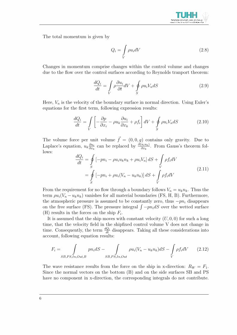
The total momentum is given by

Qi =

∫V

ρuidV (2.8)

Changes in momentum comprise changes within the control volume and changesdue to the flow over the control surfaces according to Reynolds tranport theorem:

dQi

dt=

∫V

ρ∂ui∂tdV +

∮S

ρuiVndS (2.9)

Here, Vn is the velocity of the boundary surface in normal direction. Using Euler’sequations for the first term, following expression results:

dQi

dt=

∫V

[− ∂p

∂xi− ρuk

∂ui∂xk

+ ρfi

]dV +

∮S

ρuiVndS (2.10)

The volume force per unit volume ~f = (0, 0, g) contains only gravity. Due to

Laplace’s equation, uk∂ui∂xk

can be replaced by ∂(uiuk)∂xk

. From Gauss’s theorem fol-lows:

dQi

dt=

∮S

[−pni − ρuiuknk + ρuiVn] dS +

∫V

ρfidV

=

∮S

[−pni + ρui(Vn − uknk)] dS +

∫V

ρfidV

(2.11)

From the requirement for no flow through a boundary follows Vn = uknk. Thus theterm ρui(Vn−uknk) vanishes for all material boundaries (FS, H, B). Furthermore,the atmospheric pressure is assumed to be constantly zero, thus −pni disappearson the free surface (FS). The pressure integral

∫−pnidS over the wetted surface

(H) results in the forces on the ship Fi.

It is assumed that the ship moves with constant velocity (U, 0, 0) for such a longtime, that the velocity field in the shipfixed control volume V does not change intime. Consequently, the term dQi

dtdisappears. Taking all these considerations into

account, following equation results:

Fi =

∫SB,PS,In,Out,B

pnidS −∫

SB,PS,In,Out

ρui(Vn − uknk)dS −∫V

ρfidV (2.12)

The wave resistance results from the force on the ship in x-direction: RW = F1.Since the normal vectors on the bottom (B) and on the side surfaces SB and PShave no component in x-direction, the corresponding integrals do not contribute.

6

The gravity term∫VρfidV appears only for F3. Thus the wave resistance results

in:

RW =

∫In,Out

pn1dS +

∫SB,PS,In,Out

ρu(Vn − uknk)dS (2.13)

Afterwards the boundary velocity in normal direction Vn = Un1 and the differentnormal vector components n1 of the surfaces (see figure 2.2) are inserted:

RW =

∫In

pdS −∫Out

pdS −∫In

ρu(U − u)dS +

∫Out

ρu(U − u)dS

+

∫SB

ρ u v dS −∫PS

ρ u v dS

(2.14)

Assuming that the side surfaces SB and PS are sufficient far away, there is noflow through them. Thus the last two terms in equation 2.14 disappear. The inletsurface is located so far in front of the ship, that the still water is undisturbed.Thus the flow velocities ui are zero on the inlet surface, so that only the pressureterm remains.

RW =

∫In

pdS −∫Out

pdS +

∫Out

ρu(U − u)dS

=

∫In

pdS −∫Out

[p+ ρu(U − u)] dS

(2.15)

The pressure is derived from Bernoulli’s equation:

p = −ρgz +1

2ρ(2Uu− u2 − v2 − w2) (2.16)

For the inlet surface the term results to −ρgz due to the zero velocities.Inserting the term for the pressure, following transformation can be carried out:

RW =

∫In

−ρgzdS +

∫Out

[ρgz − 1

2ρ(2Uu− u2 − v2 − w2) + ρ(Uu− u2)

]dS

=

∫In

−ρgzdS

︸ ︷︷ ︸inlet

+

∫Out

[ρgz +

1

2ρ(−u2 + v2 + w2)

]dS

︸ ︷︷ ︸outlet

(2.17)The equation can be simplified further by introducing the boundaries of the inletand outlet surfaces. Both surfaces are planes with constant x and breadth B. Sothe boundaries in y-direction are -B/2 and B/2. In z-direction they are boundedby the bottom at z = h and the free surface at z = ζ. At the inlet the wave elevation

7

is zero (ζ = 0). It follows:

RW =

B/2∫−B/2

h∫0

−ρgzdzdy

︸ ︷︷ ︸inlet

+

B/2∫−B/2

h∫ζ

ρgzdzdy +

B/2∫−B/2

h∫ζ

1

2ρ(−u2 + v2 + w2)dzdy

︸ ︷︷ ︸outlet

= ρg

B/2∫−B/2

0∫ζ

zdzdy +1

2ρ

B/2∫−B/2

h∫ζ

(−u2 + v2 + w2)dzdy

(2.18)Finally, the wave resistance formula results in:

RW =1

2ρg

B/2∫−B/2

ζ2dy +1

2ρ

B/2∫−B/2

h∫ζ

(−u2 + v2 + w2)dzdy (2.19)

This equation is generally valid in potential flow regardless of the x-position of therear boundary. The only requirement is that the control volume is wide enough,so that no waves pass through the sides.

Equation 2.19 serves for the deduction of transverse wave cut analysis. Analternative expression for wave resistance can be received by moving the inlet andoutlet surfaces infinitely far in front and astern, respectively. Then the entireenergy flows over the side boundaries. Starting with equation 2.14, the waveresistance results in:

RW = ρ

∫SB

u v dS − ρ∫PS

u v dS (2.20)

This formulation leads to longitudinal wave cut analysis. However, the infinitelength of the control surfaces creates difficulties. Thus in the first instance atransverse cut approach is prefered.

2.3 Potential Flow

Potential theory is used to describe the fluid domain exterior to a floating body.The assumption of an irrotational flow constitues an inviscid fluid. Therefore

viscous effects are not covered by potential flow theory.Implying the previous conditions, the velocity vector field is descibed by a scalar

potential Φ(x,y,z):~u = ∇Φ (2.21)

The searched velocity potential combines the conservation of mass and of mo-mentum. The balance equations matche Laplace’s equation:

∆Φ = 0 (2.22)

8

The conservation of energy is covered by Bernoulli’s equation. The velocity po-tential is determined by solving Laplace’s equation in consideration of followingboundary conditions.

There is no flow through the hull surface y = η(x,z). Therefore following Neu-mann condition requires tangential velocities on the hull surface.

~n · ∇Φ(x,η,z) = 0 (2.23)

Thereby ~n represents the normal vector of the hull surface. On the free surfacez = ζ(x,y) the kinematic condition

~n · ∇Φ(x,y,ζ) = 0 (2.24)

and the dynamic condition

2gζ +∇Φ(x,y,ζ)2 = U2 (2.25)

have to be satisfied. The kinematic condition prohibits flow through the free sur-face. Here ~n is the normal vector of the free surface. The dynamic conditionexpresses constancy of pressure using Bernoulli’s equation. This pair of bound-ary conditions are called Stokes condition, according to non-linear Stokes waves.Additional conditions are the requirement for no flow through the bottom z = hof the water and a radiation condition. The last one demands that any waves liebehind the ship, so that the ship advances into still water.

Solving this non-linear boundary-value problem, the velocity potential is known.Then the pressure distribution and the location of the free surface can be deter-mined. The pressure is calculated from Bernoulli’s equation:

p(x,y,z) =1

2g

(U2 −∇Φ(x,y,z)2

)+ ρgz (2.26)

The equation for the free surface is derived as well from Bernoulli’s equation,according to the dynamic free surface condition:

ζ(x,y) =1

2g

(∇Φ(x,y,ζ)2 − U2

)(2.27)

Therefor the potential Φ has to be evaluated at the water surface. Yet, initiallythe location of the free surface is unknown. For that reason, the location has tobe determined interatively (cf. section 4.2).

9

3 Review of Previous Work

In the following chapter, different approaches of wave cut analysis in literature arepresented. The nomenclature of the shown formulas from different publications isadapted so that consistency is warranted.

A(α) Rw

I

IIa

IIb

Fourier

analysis

∫A2(α)cos3αdα

semi-empiricalfactors ∫

AB

ζ2,etc.ds

Figure 3.1: Classification of wave cut analysis methods

A classification of the different methods according to Ward [7] is shown in figure3.1. Methods can be assigned to two ways: I and II. The first one determines afree wave spectrum by Fourier analysis from the wave elevation data. Then thewave resistance is calculated from the spectrum. These methods can be devidedmainly into transverse and longitudinal wave cut analysis.

Way II is subdivided into two paths. Path IIa requires only an integration overthe squares of the wave elevations. Path IIb integrates the forces acting on avertical cylinder (XY method). However, semi-empirical approaches, belonging tothe first subdivision, turned out to be inapplicable. Table 3.1 gives an overview ofthe authors and their published methods.

10

author references methodI Eggers [8], [9], [10], TWC method

([11], [12])Sharma [13] TWC and LWC methodsNewman [14] LWC methodShor [15] LWC methodPien [16] LWC methodKajitani [17] LWC methodGadd,Hogben [18], [12] Fourier strip method

[19], [12] matrix methodWehausen [20] TWC and LWC methodsSoding [21], [22] transverse/matrix method

II a Korvin,KroukovskyWardKajitaniGadd,Hogben [18] mean-square method

II b Ward [7], [23] XY method

Table 3.1: Review of wave cut analysis

The basic idea of wave cut analysis is to attribute a wave resistance to givenwave pattern without explicit reference to the cause of wave making. This ideawas first investigated by Havelock in 1934 [24]. He is not listed in the table above,due to the lack of instructions for the determination of the coefficients, describingthe wave pattern. However, in literature many references to his wave resistanceformula can be found. Thus his basic idea is described in section 3.1.

A proposal by Inui (1955) and a suggestion by Korvin and Kroukovsky (1960)can be regarded as the origin of the development of wave cut analysis [9]. Accordingto Michelsen and Uberoi [25], the first wave cut method, which uses wave cuts tocalculate the wave resistance, was presented by Eggers in 1962. Although Eggersdescribes as well the computation of the wave resistance using a measured wavecut parallel to the tank wall, the emphasis of this work was placed on a transversecut method. Transverse wave cut methods are presented in section 3.2.

However, provided that the wave elevation data are taken from measured wavecuts during model tests, in practice transverse wave cut methods have some dis-advantages. First, elaborate measurements are necessary to determine multipleprofiles in a moving coordinate system. Secondly, the transverse cuts cross thewake where viscous effects are significant. This violates basic assumptions of thetheory.

Thus there have been several publications of longitudinal wave cut methods.No less than five papers can be found in the proceedings of the InternationalSeminar of Theoretical Wave Resistance in 1963. Longitudinal wave cut methods

11

are introduced in section 3.3.Due to minor relevance, the Fourier strip method and the matrix method from

Gadd and Hogben are not described further. In section 3.4 the XY method ispresented. Since semi-empirical methods are not taken into consideration, the XYmethod is the only method, which manages without Fourier analysis. This reducesthe calculation effort.

However, this advantage becomes less important regarding higher computing ca-pacities of modern computers. Futhermore, modern computer technology enablesthe replacement of measured wave data by computed wave fields. Based on thesolution of a potential solver, Soding implemented a wave cut analysis [22]. It isdescribed in section 3.5 and serves as starting point for the development of thewave cut method in this thesis.

3.1 Havelock

Havelock calculates the wave resistance from the examination of the flow of energyin the wave motion. In his paper from 1934 [24] he extended the method fromonly two-dimensional problems to three-dimensional fluid motion. Assuming deepwater, a plane wave advancing in a direction making an angle α with the x-axis isgiven by

ζ = a · sin(k0 sec2(α) (x cos(α) + y sin(α)− Ut cos(α))

)(3.1)

and

Φ = a · U · cos(α)e−k0z sec2(α) cos

(k0 sec2(α) (x cos(α) + y sin(α)− Ut cos(α))

)(3.2)

where k0 = g/U2.The free wave pattern is composed of plane waves advancing in all directions.Independent of the propagation angle α the wave moves steadily with velocityU in x-direction. From equation 3.1 and 3.2 it becomes apparent that the wavenumber is expresed by k = k0 sec2 α. This term fulfils the condition for progressionwith U in x-direction c = ω/k = U cosα and the deepwater dispersions relationk = ω2/g. So a steady wave pattern occurs. In addition, Havelock presumessymmetry with respect to the x-axis. For the composed wave pattern follows:

ζ = 2

π/2∫0

f(α) sin(k0x′ sec(α)) cos(k0y sin(α) sec2(α)) dα (3.3)

and

Φ = 2U

π/2∫0

f(α)e−k0z sec2(α) cos(k0x

′ sec(α)) cos(k0y sin(α) sec2(α)) cos(α) dα

(3.4)

12

where x′ = x− Ut.This flow model approach is inserted into the known formula for the flow of totalenergy across an earth fixed vertical plane with x = constant

1

2ρU

∞∫0

∞∫−∞

(∂Φ

∂x

)2

+

(∂Φ

∂y

)2

+

(∂Φ

∂z

)2

dy dz +1

2ρgU

∞∫−∞

ζ2dy (3.5)

and into the rate of work being done across the same plane

ρU

∞∫0

∞∫−∞

(∂Φ

∂x

)2

dy dz (3.6)

The results are

πρU3

π/2∫0

(f(α))2[(3− sin2(α)) sin2(k0x

′ sec(α)) + (1 + sin2(α)) cos2(k0x′ sec(α))

] cos3(α)

1 + sin2(α)dα

(3.7)for the flow of energy and

2πρU3

π/2∫0

(f(α))2 sin2(k0x′ sec(α))

cos5(α)

1 + sin2(α)dα (3.8)

for the rate of work. However, Havelock uses linearized formulas replacing ζ by 0.Thus the results are not exact.

Finally, towing power RWU (frictional resistance neglected) is determined fromthe flow of energy and the rate of work across two fixed vertical planes. One isplaced far in advance, so that there is no flow disturbance. The other plane islocated far behind the ship, where the wave pattern can be expressed by equation3.3. Thus the towing power RWU results in the substraction of equation 3.8 from3.7. For the wave resistance follows:

RW = πρU2

π/2∫0

(f(α))2 cos3(α),dα (3.9)

Alternatively, the wave pattern can be composed from sinus and cosinus compo-nents. Then the wave resistance results to:

RW = πρU2

π/2∫0

[(a(α))2 + (b(α))2

]cos3(α) dα (3.10)

13

This form is cited for example in [26] or [6]. In his paper [24] Havelock developsas well a resistance formula for finit depth:

RW = πρU2

π/2∫0

(f(α))2(

coth(kh)− kh

sinh2(kh)

)cos3(α) dα (3.11)

Basically, Havelock describes a suitable flow model for wave pattern of a shipand deduces a formula for the related wave resistance. However, since Havelockdoesn’t give instructions for the calculation of the wave components f(α) of thewave pattern, his work cannot be regarded as a complete wave cut method.

3.2 Transverse wave cut analysis

The first transverse wave cut analysis was presented by Eggers in 1962. All subse-quent publications of transverse wave cut analysis are basically similar. Thus thefollowing section is based on Eggers inital paper [8]. A translation of the paperwas published in the proceedings of the International Seminar on Theoretical WaveResistance [27].

Eggers develops a method to determine the wave resistance. Alternatively toFroude’s method, the wave resistance is calculated from measured wave profilesin a canal. First Eggers deduces a linearized form of the wave resistance formulagiven in equation 2.19:

RW =1

2ρg

B/2∫−B/2

ζ2dy +1

2ρ

B/2∫−B/2

h∫0

(−Φ2x + Φ2

y + Φ2z)dzdy (3.12)

For the deviation Eggers considers energy balance in control volume bounded bythe canal walls and a front and a rear plane. Then an approach for the velocitypotential of the wave field behind the ship is made:

Φ(x,y,z) =∑n

g

Uknx

1

cosh(knh)[an cos(knxx)− bn sin(knxx)] cosh(kn(z − h)) cos(

nπ

By)

(3.13)This approach satisfies the linearized free-surface condition. It is based on thecomposition of elementary waves with different wave numbers kn. According to aFourier analysis, the component of the wave number in y-direction is definded as:

kny =nπ

B(3.14)

Due to the dispersions relation for steady wave pattern, the wave number has tofulfil following equation:

k2n − k2ny −gknU2

tanh(knh) = 0 (3.15)

14

The velocity potential (equation 3.13) is inserted into the wave resistance formula(equation 3.12). Using the linearized wave elevation ζ = U/gΦx(x,y,0) it follows:

RW =1

2ρgB

∞∑n=−∞

(a2n + b2n)

[1− g tanh(knh)

2U2kn

(1 +

2knh

sinh(2knh)

)](3.16)

Finally, the Fourier coefficients an and bn are determined using two transverse waveprofiles. Inserting these into equation 3.16, the wave resistance can be calculated(transverse wave cut analysis).

Further, Eggers considers the cases of sideways and downwards unbounded fluid.For b→∞ the sum transforms into an integral. However, in practice a transversewave cut can be truncated at some value of y outside the Kelvin wedge, becauseoutside this area the free surface is unaffected. Indefinite depth results in a sim-plification of the wave resistance formula, due to the use of deepwater dispersionsrelation.

In addition, Eggers shows that the derived wave resistance expression (equa-tion 3.16) corresponds to the energy flow of composed plane waves with differentpropagation angle α to the x-axis. This interpretation equals Havelocks conceptof composition the wave pattern from plane waves (concept of free wave system).

Descriptions of transverse wave cut methods can be found in surveys on wavecut analysis or wave resistance by Eggers, Sharma and Ward [9], by Wehausen[20], and by Eggers [10]. Applications of the methods are published by Sharma[13], by Gadd and Hogben [12] and by Mizuno and Wehausen [11].

Wehausen gives a detailed deduction of equation 3.12. The procedure is similarto the one in section 2.2 with the difference that viscosity is taken into account byWehausen. Thus instead of Euler’s equations Navier-Stokes equations are used.However, the assumption of irrotational flow and of inviscid fluid leads finally tothe same resistance formula. Transverse wave cut techniques are considered formeasured profiles in a canal and for profiles in unbounded fluid. In contrast toEggers (equation 3.13), his approach of the velocity potential includes an additionalexponential term:

Φ(x,y,z) =∑n

g

Uknx

1

cosh(knh)[−an cos(knxx) + bn sin(knxx)] cosh(kn(z − h)) cos(

nπ

By)

+∑n,p

g

Uknxp

1

cosh(knphcnp)e

knxpx cos(knp(z − h)) cos(nπ

By)

(3.17)However, the coefficient cnp does not contribute to the wave resistance formula.Thus Wehausen receives the same formula as Eggers (equation 3.16). Assumingthat the x-positions of the transverse wave cuts are far enough behing the ship,the exponential term is neglected for the Fourier analysis of the wave pattern.

Wehausen deduces, like Eggers, the coefficient determination from two trans-verse wave cuts. Instead, wave elevation and slope at one x-position can be used.

15

Alternatively, an and bn are calculated from a greater number of wave profiles byleast squares method.

3.3 Longitudinal wave cut analysis

The technical advantage of longitudinal over transverse pofiles is the easy mea-surement. A fixed wave gauge can measure the wave elevation during the passageof the ship. Obviously this argument is no longer valid when wave cut analysis isapplied to calculated wave fields.

Longitudinal wave cut methods use one or more infinitely long wave cuts parallelto the ship’s track. Assuming symmetric flow, only one longitudinal profile isneeded. The procedure is similar to the transverse cut techniques. However, thegeneral potential approach is inserted into equation 2.20 instead in equation 2.19.This equation is deduced from momentum consideration moving front and rearcontrol surface into infinity. Alternatively, the free wave spectrum with respect topropagation angle α can be determined. The resistance is then calculated fromHavelock’s formula (equation 3.10).

There are several publications relating to longitudinal wave cut techniques. Dif-ferent approches are presented during the International Seminar on TheoreticalWave-Resistance in 1963. According to Michelsen and Uberoi [25], Sharma [13]and Newman [14] presented mathematically equivalent methods. Besides papersby Pien [16],Kajitani [17] and Shor [15] are presented. The last three have thecomposition of wave pattern by a bow and a stern free wave system in common.However, they are not considered any further in later state of the art surveys onwave resistance ([9], [20], [10]).

Thus in the following, Sharma’s method is presented as a representative. Thedescription follows Heimann, who used the longitudinal wave analyis for CFDbased optimization of wave-making characteristics [26], [28].

Below non-dimensional quantities are used. These are common in many publi-cations. Length related measures are normalized by the basic wavenumber:

k0 =g

U2(3.18)

Thus non-dimensional coordinates, for example x′ = k0x, and non-dimensionalwave height ζ ′ = k0ζ are used. The wave resistance is nondimensionalized by R′W =RW · k20/(ρU2). A simple correlation between the non-dimensional wavenumber k′

and α is found by inserting the dispersion relation for deep water k = ω2/g in thecondition for a steady wave pattern c = U cosα:

k′ = sec2(α) (3.19)

The separation of the wave number into x and y components leads to:

k′x = k′ cos(α) = sec(α) (3.20)

16

k′y = k′ sin(α) = sec(α) tan(α) (3.21)

The non-dimensional transverse wavenumber can be expressed in terms of thenon-dimensional longitudinal wavenumber:

k′y = k′x√k′2x − 1 (3.22)

The wave elevation is given by the superposition of the free waves. It can beexpressed in terms of the propagation angle α (equation 3.23) or in terms of thelongitudinal wavenumber k′x (equation 3.24).

ζ(x,y) =

∫ π/2

0

[a(α) cos(k′xx+ k′yy) + b(α) sin(k′xx+ k′yy)

]dα (3.23)

ζ(x,y) =

∫ ∞1

[a(k′x) cos(k′xx+ k′yy) + b(k′x) sin(k′xx+ k′yy)

] dαdk′x

dk′x (3.24)

Equation 3.24 can be rearranged to

ζ(x,y) =

∫ ∞1

[(a(k′x) cos(k′yy) + b(k′x) sin(k′yy)

)cos(k′xx)

+(b(k′x) cos(k′yy)− a(k′x) sin(k′yy)

)sin(k′xx)

] dαdk′x

dk′x

(3.25)

Introducing the Fourier transforms

S(k′x) =

∫ ∞−∞

ζ(x,y) sin(k′xx)dx

C(k′x) =

∫ ∞−∞

ζ(x,y) cos(k′xx)dx,

(3.26)

the wave elevation can be expressed by the following continous Fourier integral:

ζ(x,y) =1

π

∫ ∞1

[S(k′x) sin(k′xx) + C(k′x) cos(k′xx)] dk′x (3.27)

Equation 3.25 is equated with equation 3.27. Followed by a separation of variables,a correlation between the Fourier transforms and the components of the free wavespectrum is found:

S(k′x) = π(b(α) cos(k′yy)− a(α) sin(k′yy)

) dαdk′x

C(k′x) = π(a(α) cos(k′yy) + b(α) sin(k′yy)

) dαdk′x

(3.28)

Resolving 3.28 for a(α) and b(α) finally results in:

a(α) =1

π

(C(k′x) cos(k′yy)− S(k′x)sin(k′yy)

) dk′xdα

b(α) =1

π

(S(k′x) cos(k′yy) + C(k′x)sin(k′yy)

) dk′xdα

(3.29)

17

The non-dimensional wave resistance can be calculated either from the Fouriertransforms:

R′W =1

π

∞∫1

[S2(k′x) + C2(k′x)

] 1

k′x

√1− 1

k′2xdk′x (3.30)

or alternatively from free wave spectrum according to Havelock:

R′W = π

π/2∫0

[a2(α) + b2(α)

]cos3(α)dα (3.31)

So the Fourier transforms (equation 3.28) have to be determined to calculate thewave resistance. The integrals can be evaluated numerically using measured orcalculated longitudinal profiles. However, the record lenght of the profile is limited.To compensate the error due to the truncation a correction has to be made.

Such a truncation correction is described for example in [9]. It is based on ananalytical asymptotic extension:

ζ ′ ≈ c1 cos(x′)− c2 sin(x′)√c3 + x′

(3.32)

In order to use this truncation correction, weighted Fourier transforms are intro-duced:

S ′(k′x) =

∫ xE

−∞

√(k′x)

2 − 1 ζ ′ sin(k′xx)dx+

∫ ∞xE

√(k′x)

2 − 1 ζ(x,y) sin(k′xx)dx

C ′(k′x) =

∫ xE

−∞

√(k′x)

2 − 1 ζ ′ cos(k′xx)dx+

∫ ∞xE

√(k′x)

2 − 1 ζ(x,y) cos(k′xx)dx

(3.33)A correction for the upstream edge is not necessary, because of the zero waveelevations at a certain distance in front of the bow. The evaluation of the firstintegral (equation 3.33) by means of complementary Fresnel integrals is given in[9]. The free wave spectrum results in:

a(α) =k′xπ

(C ′(k′x) cos(k′yy)− S ′(k′x)sin(k′yy)

)b(α) =

k′xπ

(S ′(k′x) cos(k′yy) + C ′(k′x)sin(k′yy)

) (3.34)

Besides the application of Sharma’s method in [26], a modified Newman’s methodis described and used by Michelsen and Uberoi [25]. Of course, longitudinal meth-ods are presented as well in state of the art surveys on wave cut analysis ([9], [20],[10]).

18

3.4 XY Method

The XY method determine the wave resistance from measured forces in x andy-direction (X and Y) acting on a vertical cylinder. According to linearized theoryof water-wave diffraction in an inviscid fluid, the forces are assumed to be propor-tional to the wave amplitudes. In contrast to previously presented methods, theXY method manages without Fourier analysis. Whereby the calculation effort isreduced.

The postition of the cylinder in the tank can be seen in figure 3.2. It has to beunaffected by the reflection from the tank wall.

A

B C

D x

y

XY

cylinder

reflexted wave

tank side

tank centerline

model path

Figure 3.2: XY method geometry

The basic idea is to receive the energy flux across the line BC from the integratedproduct of the X and Y signals. To determine the wave resistance, in addition, theenergy flux across AB is needed. Assuming that in this region the wave systemcan be represented by a single plane wave (with propagation angle α = 0), theenergy flux is calculated from the measured wave height at one point.

More complete descriptions of the XY method can be found in publications byWard 1963 [23] and 1966 [7]. The method is introduced as well in surveys on wavecut analysis ([9], [20], [10]).

3.5 Soding

Soding implemented a kind of multiple transverse wave cut method, which is pre-sented in [21] and in [22]. His method is starting point for the implementationof the wave cut analysis as part of this work. In the following, his method isdescribed.

19

As already Havelock did, the wave pattern behind the ship is superimposed fromregular waves according to linear wave theory. These are plane waves of differentwavenumbers k and directions of propagation α with −90◦ ≤ α ≤ 90◦. Negativeor positive angles provide waves propagating to port side or starbord, respectively.In order that a steady wave field arises, every plane wave has to fulfil the followingequation:

c = U cos(α) (3.35)

Waves, which satisfy this condition, are called free waves. They constitute the freewave spectrum.

Typical for Fourier decomposition is the calculation of 2 N coefficients from 2 Nequidistantly distributed grid points. For this reason, the wave field is approxi-mated as:

ζ(x,y) =

N/2∑n=−N/2

an cos (kn(x cos(αn) + y sin(αn)))

+

N/2−1∑n=−N/2+1

bn sin (kn(x cos(αn) + y sin(αn)))

(3.36)

There are N+1 coefficients from cosinus term and N-1 from sinus term. This is atotal sum of 2 N coefficients. However, the total number and distribution of gridpoints don’t fulfil the typical Fourier decomposition [29]. The limits of the sumscan be changed without effect on the wave resistance results.

Therefore, in the following, the limits of the second sum are changed to -N/2and N/2. This simplifies the notation. Thus the wave field results to:

ζ(x,y) =

N/2∑n=−N/2

an cos (kn(x cos(αn) + y sin(αn)))+bn sin (kn(x cos(αn) + y sin(αn)))

(3.37)Introducing the components of the wavenumbers into x and y-direction

kx = k cos(α) (3.38)

ky = k sin(α) (3.39)

and the abbrevation βn = knxx+ knyy, following equation is obtained:

ζ(x,y) =

N/2∑n=−N/2

an cos (βn) + bn sin (βn) (3.40)

From equation 3.38 and 3.39 follows:

k =√k2x + k2y (3.41)

20

For the determination of the Fourier coefficients, Soding uses a least squaresmethod based on the wave heights in a rectangle behind the ship. Therefor hetakes the wave elevation values at the free surface grid points as computed by theRankine source method.

Conforming a Fourier development, the component in y-direction of the wavenum-ber (cf. equation 3.39) varies in constant steps:

ky =2πn

Bwith n = −N

2...N

2(3.42)

Thereby N is the number of grid cells within each transverse cut with breadth B.With the help of the dispersion relation for shallow-water the correlation between

k and α is derived:

c =ω

k=√g/k · tanh(kh) = U cos(α) (3.43)

Using this dispersions relation for steady wave pattern, equation 3.39, and cos2 αn =1− sin2 αn, following equation results:

F 2

[knh−

(knyh)2

knh

]= tanh(knh) (3.44)

where F 2 = U2/gh is the square of the depth Froude number. Only sub-criticaldepth Froude numbers are assumed (0 < F < 1). Solving equation 3.44 by intera-tion for knh, a wave number kn is determined for every n or kny. The correspondentknx is calculated from equation 3.41. Then the Fourier coefficients an and bn canbe determined by least square method:

minimize∑k

(ζk − ζk)2 (3.45)

ζk are the wave heights at the grid points, taken from potential solver solution.Inserting equation 3.40 and differentiating with respect to aj and bj, followingequation system is received:

∑k

N/2∑n=−N/2

an cos(βnk) + bn sin(βnk)− ζk

cos(βjk) = 0

∑k

N/2∑n=−N/2

an cos(βnk) + bn sin(βnk)− ζk

sin(βjk) = 0

(3.46)

where j = −N/2 ... N/2

21

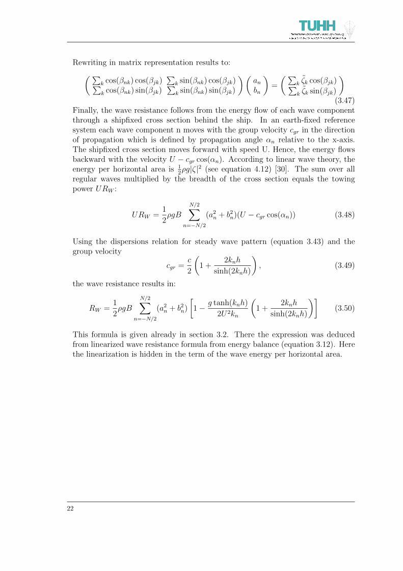
Rewriting in matrix representation results to:(∑k cos(βnk) cos(βjk)

∑k sin(βnk) cos(βjk)∑

k cos(βnk) sin(βjk)∑

k sin(βnk) sin(βjk)

)(anbn

)=

(∑k ζk cos(βjk)∑k ζk sin(βjk)

)(3.47)

Finally, the wave resistance follows from the energy flow of each wave componentthrough a shipfixed cross section behind the ship. In an earth-fixed referencesystem each wave component n moves with the group velocity cgr in the directionof propagation which is defined by propagation angle αn relative to the x-axis.The shipfixed cross section moves forward with speed U. Hence, the energy flowsbackward with the velocity U − cgr cos(αn). According to linear wave theory, theenergy per horizontal area is 1

2ρg|ζ|2 (see equation 4.12) [30]. The sum over all

regular waves multiplied by the breadth of the cross section equals the towingpower URW :

URW =1

2ρgB

N/2∑n=−N/2

(a2n + b2n)(U − cgr cos(αn)) (3.48)

Using the dispersions relation for steady wave pattern (equation 3.43) and thegroup velocity

cgr =c

2

(1 +

2knh

sinh(2knh)

), (3.49)

the wave resistance results in:

RW =1

2ρgB

N/2∑n=−N/2

(a2n + b2n)

[1− g tanh(knh)

2U2kn

(1 +

2knh

sinh(2knh)

)](3.50)

This formula is given already in section 3.2. There the expression was deducedfrom linearized wave resistance formula from energy balance (equation 3.12). Herethe linearization is hidden in the term of the wave energy per horizontal area.

22

4 Implementation of a Wave Cut Analysis

In this chapter the implemented wave cut analysis is described. Starting point forthe development is a wave cut routine according to Soding [21], which is alreadyavailable at the Institute of Ship Design and Ship Safety [31]. Soding’s originalmethod is described in detail in section 3.5.

The wave field is taken from a non-linear Rankine source method. The usedin-house potential method MINK [31] provides the computed velocity potentialand the wave elevation at every grid point of the free surface discretization.

4.1 Outline of Current Work

Basically, following improvements of the wave cut method according to Soding aremade:

• The wave elevations are calculated by Newton’s method at freely choosablepositions.

• The number of Fourier coefficients is defined independently of the number ofgrid points per wave cut.

• The non-linear part of kinetic wave energy is taken into account.

Resulting from point one and two, the number and position of grid points and thenumber of Fourier coefficients are no longer predefined by the used surface grid ofthe potential solver. Thus investigations of the needed number of grid points andFourier coefficients are made.

Furthermore, an alternative calculation of the Fourier coefficients is implemented.This enables the user to detect inadequate resistance calculations, for example dueto inappropriate wave cut positions, more easily.

To show the effects of the improvements on the calculated wave resistances, re-sults from different levels of implementations are compared (see section 5). There-fore resistances according to the following methods are computed. In the intro-duced abbrevations TWCA stands for transverse wave cut analysis. The F indi-cates the use of a Fourier analysis.

Soding’s original TWC analysis (TWCAF Soe)

The original method implemented by Soding uses the wave elevation values at thegrid points which are provided from Rankine source method in a rectangle behindthe ship. To recreate this method, the wave cut grid points are located at locationsof potential solver grid point. Yet, the spacing of the near field behind the shipis not exactly the same as the one of the far field. Thus the equidistant wave cutgrid points don’t fit the exact positions of the near field grid points of the potentialsolver.

23

The choosen rectangle has a lenght of one wavelength and is placed the lenghtof two cells in front of the aft end of the discretized area of the potential solver.

According to Soding [21], the number of Fourier coefficients is equal to thenumber of grid points per transverse wave cut. After calculating the coefficients byleast squares method, the wave resistance is determined by linear wave resistanceformula (equation 3.50).

Linear TWC analysis (TWCAF lin)

In contrast to Soding’s original method, this method allows to choose the numberof the transverse wave cuts as well as the number of grid points per wave cut (seesection 4.3). Besides, the number of calculated Fourier coefficients is independentof the number of grid points (see section 4.4). The calculation of the coefficientsand wave resistance corresponds with Soding’s original method.

TWC analysis (TWCAF)

The third improvement changes the wave resistance computation. The non-linearTWC method calculates the wave resistance in consideration of non-linearizedmean kinetic wave energy. This is described in section 4.5. In addition, as describedin section 4.4, an alternative Fourier coefficient calculation method is implemented.

Direct evaluation of the velocity potential (TWCAP)

In addition to the three transverse wave cut methods based on a flow model usinga Fourier analysis, a direct evaluation of the velocity potential based on equation2.19 is implemented. This method is more time-consuming, however, it is suitablefor verification of the results from the wave cut analysis. The implementation isdescribed in section 4.6.1.

Pressure integration

The pressure integration is carried out from the potential solver MINK. The waveresistance is calculated from integration of the pressure over the hull which isdiscretized by patches.

As an alternative approach to transverse wave cut analysis, a longitudinal wavecut method is implemented. Yet, this method is not developed further. The gainedknowledge can be found in section 4.6.2.

24

4.2 Wave Heights Computation by Newton’s Method

As mentioned above, the wave field of the examined ship is determined by usingthe in-house potential method MINK. The wave heights at the grid points of thewave cuts are calculated from the received potential.

Form Bernoulli’s equation at the free surface follows:

ζ(x,y) =1

2g(U2 − (∇Φ(x,y,ζ))2)) (4.1)

Thus the potential Φ has to be evaluated at the water surface. Yet, initially theposition of the surface is unknown. For that reason the position is determined in-teratively. Therefor a bisection method is available [31]. However, the convergencebehaviour is relative poor (cf. figure 4.2). For this reason, a Newton’s method isimplemented alternatively.

Newton’s method is a fixed-point procedure for computing zeros of a functionf(x). The point xk shall be assumed to lie near a zero. A point xk+1 closer tothe zero results from the intersection of the tangent to f(xk) and the x-axis. Thiscorrelation is given in equation 4.2.

xk+1 = xk −f(xk)

f ′(xk)(4.2)

Commencing at a start point x0, the iteration is carried out until either a definedtolerance or the maximum number of iterations is reached.

x

f(x)

x0x1x2

Figure 4.1: Newton’s method

In case of the iteration of the water surface ζ, the zero of the function f(ζ) (seeequation 4.3) is searched. The function f(ζ) results form equation 4.1.

f(ζ) = ζ − 1

2g(U2 − (∇Φ)2))

!= 0 (4.3)

25

According to equation 4.2, the first order derivative of f(ζ) with respect to ζ isneeded.

f ′(ζ) = 1 +1

2g

δ

δζ(∇Φ)2 (4.4)

The needed derivatives of the gradient of the potential with respect to the waveheight are determined using a finite difference method. Chosen is a ∆ζ of onemillimeter. The formulation according to equation 4.5 has a first order exactness.

δ

δζ(∇Φ(ζ))2 =

(∇Φ(ζ + ∆ζ))2 − (∇Φ(ζ))2

∆ζ(4.5)

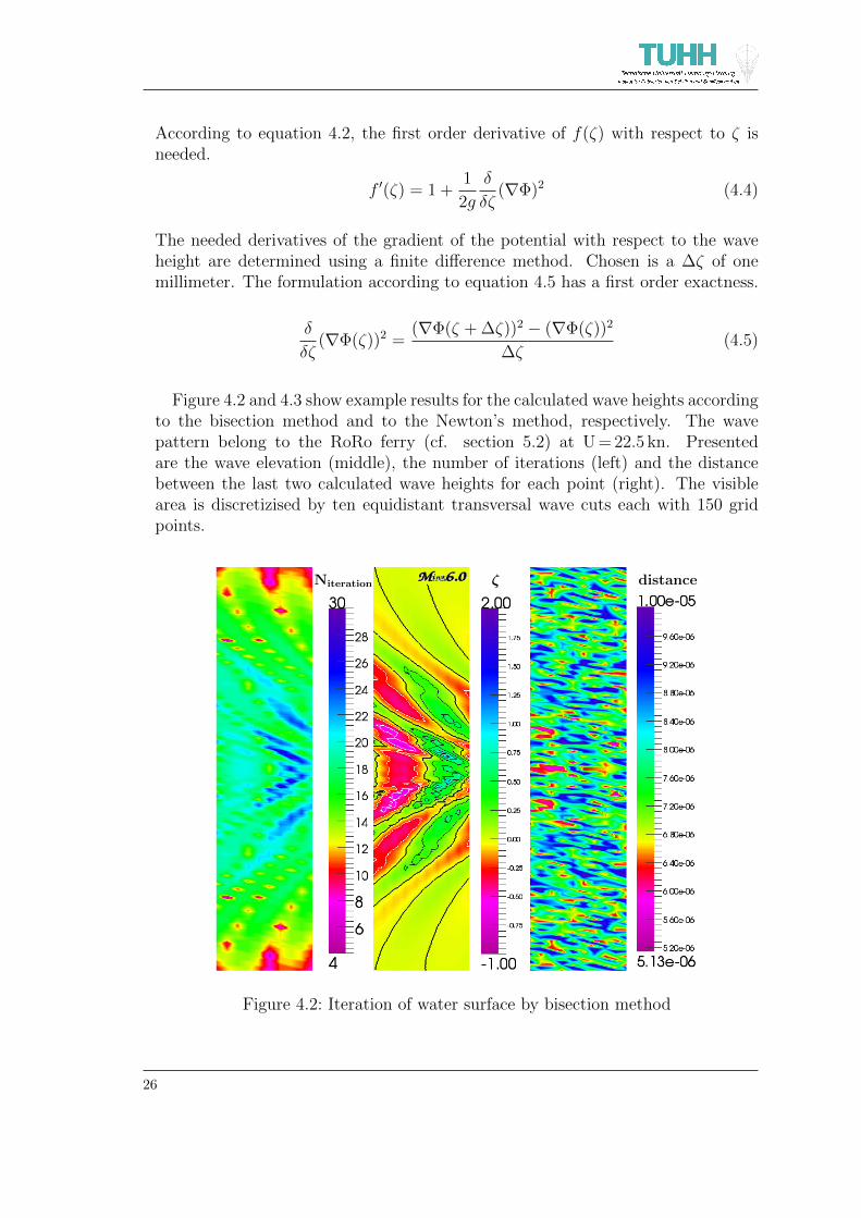
Figure 4.2 and 4.3 show example results for the calculated wave heights accordingto the bisection method and to the Newton’s method, respectively. The wavepattern belong to the RoRo ferry (cf. section 5.2) at U = 22.5 kn. Presentedare the wave elevation (middle), the number of iterations (left) and the distancebetween the last two calculated wave heights for each point (right). The visiblearea is discretizised by ten equidistant transversal wave cuts each with 150 gridpoints.

Niteration ζ distance

Figure 4.2: Iteration of water surface by bisection method

26

Niteration ζ distance

Figure 4.3: Iteration of water surface by Newton’s method

The good convergence of the Newton’s method becomes apparent by comparingthe needed numbers of iteration of both methods. Maximal four iterations areneeded by Newton’s method to fulfil a tolerance of 1 · 10−5 m. In contrast, thebisection method needs between four and 30 iterations.

27

4.3 Discretization and Position of Transverse Wave Cuts

According to a transverse wave cut method, Soding uses a Fourier analysis ap-proach in y-direction for the determination of the free wave spectrum. He calcu-lates the fourier coefficients by a least squares method based on the wave heightsin a rectangle behind the ship. Therefor Soding takes the wave elevation valuesat the free surface grid points as computed by the Rankine source method. Anexample is shown in figure 4.4. The analysis rectangle is marked in grey.

Figure 4.4: Wave field example according to Soding (taken from [21]).

As a result, the accuracy of the wave field reconstruction depends on the resolutionof the free surface of the potential method. To avoid this, the implemented wave cutanalysis calculates the wave elevation for defined points from the velocity potential(cf. section 4.2). By doing so, the longitudinal positions of the transverse cuts andthe numbers of grid points per cut are arbitrarily choosable.

In the following, the requiered number of grid points and their arrangementbehind the ship are investigated. The grid for the computation of the Fouriercoefficients consists of multiple transverse wave cuts. Each transverse wave cut isdiscretizised by a defined number of grid points. The grid points are distributedequidistantly.

The transverse wave cuts have to be located so far behind the stern that theinfluence of near field disturbances are negligible. Experience values can be foundin literature. Soding [22] recommends a distance of about one breadth of the shipbetween stern and first wave cut. In [3], based on experiences, 0.3 to 0.5 Lpp ismentioned. However, further investigations had shown that non-linear effects maypersist behind the ship for a distance of about two times the ship’s lenght. There-fore a spreading of the wave cuts over one fundamental wavelength is proposed in[3]. Soding demands a spreading over at least 85 % of one wavelength.

If the discretizised surface area of the potential solver is large enough, the trans-verse wave cuts are spreaded over one wavelenght. The distance between the first

28

wave cut and the stern amounts at least 75 % of one wavelength. The distanceis increased as far as possible. The last wave cut (most downstream) is located asmall distance in front of the aft end of the discretizised surface area (cf. [21]).

Figure 4.5 shows an example of the wave field calculated from Rankine sourcemethod MINK and the location of the transverse wave cuts in the discretizisedsurface area. The pictured control area is explained below.

control area

λ

≤ 0.75λ

0.5λ

TWC

ζ

Figure 4.5: Transverse wave cuts and control area.

The wave cuts are equidistantly distributed in x-direction. They expand in y-direction over the whole breadth of the discretizised area. In the following, thenumber of transverse wave cuts and the number of grid points per wave cut haveto be specified.

For the investigation of the optimal number of wave cuts and grid points thefollowing goals can be formulated:

• In order to reduce computing time, the total number of grid points shouldbe as low as possible.

• The Fourier coefficients, which are calculated from the transverse wave cuts,should reconstruct the wave field of the ship as precisely as possible.

29

To evaluate the satisfaction of the second item, a control area is defined (see figure4.5). In this control area wave elevations on equidistant grid points are calculatedfrom the derived Fourier coefficients (equation 3.40). These flow model wave eleva-tions are compared with the wave elevations from the velocity potential calculatedby Newton’s method (see section 4.2). The mean amount of the differences istaken as evaluation criterion. Known from experience, high or low mean valuescorrespond with high or low maximum values, respectively.

Satisfactory resistance results correspond with mean values smaller than 0.02 m.However, a generally valid recommendation for choosing the number of wave cutsand grid points cannot be made. Yet computing times are relatively small, so thata high number of grid points, for example 150, can be choosen. It seems that thenumber of Fourier coefficients is an indicator of an sufficient number of grid points.A suitable number of wave cuts is 10.

However, at certain cases numerical problems at Fourier coefficient calculationoccur, if the spacing between the wave cuts is unfavorable (see section 4.4). Thenthe number of wave cuts should be changed.

The mentioned experiences and values are based on on only two test cases (seesection 5). A different ship or a greater free surface domain may requiere moregrid points or wave cuts. This can be tested by comparing wave resistance resultsof calculations with different resolutions.

4.4 Fourier Coefficients Calculation and Free Wave Spectrum

After calculating the wave elevation on every grid point of the transverse wave cuts,the wave field is reconstructed by elementary waves. These free waves constitutethe free wave spectrum. There are two different implemented methods to determinethe Fourier coefficients from the wave cuts.

The first one is the least square method according to Soding described in section3.5. The second one carries out a Fourier analysis for every wave cut. The waveelevation according to equation 3.37 can be rewriten as:

ζ(x,y) =

N/2∑n=−N/2

[an cos(knxx) + bn sin(knxx)] cos(knyy)

+[bn cos(knxx)− an(knxx)] sin(knyy)

(4.6)

The Fourier coefficients are calculated by evaluating equations 4.7 and 4.8 usingtrapezodial rule and solving for an and bn. Then mean coefficients are determinedby least squares method using all wave cut points.

an cos(knxx) + bn sin(knxx) =1

B

B/2∫−B/2

ζ cos(knyy)dy (4.7)

30

bn cos(knxx)− an(knxx) =1

B

B/2∫−B/2

ζ sin(knyy)dy (4.8)

If the linear equation system of the first method (equation 3.47) is well-conditionedand each wave cut is discretized by enough grid points, both methods determinethe same Fourier coefficients. However, at certain spacings between the wave cutsnumerical problems solving the equation system can occur. These lead to unreal-istic wave resistance results.

The second method seems to be more complicated. Yet, numberical problemsduring the least squares fit can be detected more easily. By calculating the af-fected Fourier coefficients by averaging arithmetically instead of using least squaresmethod, the wave resistance error can be kept small. However, a second calculationwith a different number of wave cuts should be carried out.

Experience showed, that a wave resistance seems to be reliable, if both meth-ods calculate the same value for the wave resistance. In addition, the free wavespectrum can be checked for runaway coefficients.

Figure 4.6 shows two example free wave spectra calculated from the wave fieldof the Wigley hull (see section 5.1). The spectra belong to different Froude num-bers. In both cases the same number of Fourier coefficients is calculated. Yet,the covered range of transverse wavenumbers or of propagation angles differs, be-cause of different breadths of the wave cuts. Theoretically, free waves up to ± 90◦

have to be considered. However, the amplitudes approach zero well before. ThusFourier coefficients have to be calculated only up to the point, where the valuesare sufficiently close to zero. From the corresponding transverse wavenumber ky,the maximum needed number of Fourier coefficients can be found (equation 3.42).

31

-0.03-0.02-0.01

00.010.020.030.04

cos

com

pon

ent

[m]

-0.12-0.1

-0.08-0.06-0.04-0.02

00.020.04

sin

com

pon

ent

[m]

-80-60-40-20

020406080

-2 -1.5 -1 -0.5 0 0.5 1 1.5 2

α[d

eg]

ky [1/m]

Fn = 0.188 Fn = 0.325

Figure 4.6: Free wave spectrum for Fn = 0.188 and Fn = 0.325

Investigations are made for the Wigley hull (see section 5.1) and for a RoRo ferry(see section 5.2). In case of the Wigley hull free wave spectra of Froude numbersfrom 0.188 to 0.400 are analyzed. For the RoRo ferry the Froude numbers are inthe range of 0.209 to 0.279. The needed number of Fourier coefficients dependson the maximal transverse wave number ky according to the free wave spectrumand on the breadth of the wave cuts or free surface domain B (cf. equation 3.42).The breadth B, in turn, depends on the length of the free surface domain inconsideration of the Kelvin angle.

Thus with increasing Froude number the breadth B increases due to longer wave-lenghts which effect longer free surface domains. On the other hand, experience

32

from evaluation of the investigated free wave spectra shows decreasing transversewave numbers at higher Froude numbers. The resulting numbers of Fourier coeffi-cients N vary in a certain range, but without a detectable trend. Hence, it can beconcluded that the described contrary effects compensate each other.

However, the received range for N differs for the Wigley hull and the RoRo ferry.For the Wigley hull the needed numbers of Fourier coefficients amounts between51 and 71. For the RoRo ferry a range of 99 to 125 is obtained. The differencecan be traced back to different values for B, due to the fact that the length of thesurface domain depends besides on the wavelenght as well on the ship’s length.Thus, for comparison, the needed number of Fourier coefficients are divided bythe length between perpendiculars Lpp. For the Wigley hull and the RoRo ferryfollows N/Lpp = 0.51...0.71 and N/Lpp = 0.52...0.66, respectively.

Based on these results, the number of Fourier coefficients is set to N = 0.71Lpp.However, this experience value is based on only two test cases. A general validityfor conventional ships has to be verified. Therefore, the number of Fourier coeffi-cients is adjustable by the user. Checking the adequacy of the choosen value canbe done relative easily by ploting the free wave spectrum.

4.5 Wave Resistance Computation

Having determined the Fourier coefficients, the wave resistance can be deducedfrom the energy flow of each wave component across a transverse plane. The waveenergy consists of potential and kinetic energy. In the following, the mean energyper horizontal area e according to linear wave theory is derived (cf. [30]). Thepotential energy is the result of lifting height and weight per area:

epot = −ζ2ρg(−ζ) =

1

2ρgζ2 (4.9)

For regular waves the wave height is given by ζ = |ζ| · sin (2π/λ · x). Here x is thecoordinate in the direction of propagation of the wave. The mean value e followsfrom averaging over one wavelength:

epot =1

λ

λ∫0

1

2ρg|ζ|2 · sin2

(2π

λx

)dx =

1

4ρg|ζ|2 (4.10)

For the kinetic energy the orbital velocities are needed. In case of deep waterwaves the absolute value of the orbital velocity amounts constantly ω|ζ|ekz (see[30]). Thus the kinetic energy results to:

ekin =

∞∫ζ

1

2ρ(u2 + w2)dz =

∞∫ζ

1

2ρω2|ζ|2e−2kzdz (4.11)

33

The term for the kinetic enery can be simplified by linearization. This results in aconstant value for the kinetic energy:

ekin ≈∞∫0

1

2ρω2|ζ|2e−2kzdz =

1

4ρg|ζ|2 ≈ Ekin (4.12)

Using this linearization the total mean wave energy leads to following familiarexpression:

E = Epot + Ekin ≈1

2ρg|ζ|2 (4.13)

This term is used by Soding for the wave resistance determination, resulting inequation 3.50. Without linearization the kinetic energy varies with respect to ζand x:

ekin =

∞∫ζ

1

2ρω2|ζ|2e−2kzdz

= −1

2ρω2

2k|ζ|2

[e−2kz

]∞ζ

=1

4ρg|ζ|2e−2k|ζ| sin(2π/λ·x)

(4.14)

The mean value is determined by averaging over one wavelength:

ekin =1

λ

λ∫0

1

4ρg|ζ|2e−2k|ζ| sin(2π/λ·x)dx (4.15)

This integral is not solvable analytically. However, it can be evaluated by numericalintegration. For the total mean wave energy follows:

e =1

4ρg|ζ|2

1 +1

λ

λ∫0

e−2k|ζ| sin(2π/λ·x)dx

(4.16)

Calculating the energy flow of the free waves according to this expression for theenergy per horizontal area, following equation results for the wave resistance:

RW =1

4ρgB

N/2∑n=−N/2

a2n1 +

1

λn

λn∫0

e−2knan cos(2π/λn·x)dx

+ b2n

1 +1

λn

λn∫0

e−2knbn sin(2π/λn·x)dx

· [1− g tanh(knh)

2U2kn

(1 +

2knh

sinh(2knh)

)](4.17)

34

Thus, after having determined the Fourier coefficients, the terms

1

λn

λn∫0

e−2knan cos(2π/λn·x)dx (4.18)

and

1

λn

λn∫0

e−2knbn sin(2π/λn·x)dx (4.19)

are solved numerically using a sufficient number of grid points for each wave com-ponent n. Finally, after determining the wave resistance, the non-dimensional wavecoefficient is calculated:

CW =RW

12ρU2Aw

(4.20)

4.6 Alternative Approaches

In the previous sections, the development of the transverse wave cut analysis isdescribed. In the following two alternative approaches are presented. The methodof direct evaluation of the velocity potential is applied to the test cases for vali-dation purposes (section 5). The longitudinal wave cut method is not developedfurther.

4.6.1 Direct evaluation of the velocity potential

The direct evaluation of the velocity potential (TWCAP) is based on the evaluationof equation 2.19. Therefore the velocity potential, which is given by the potentialsolver MINK, is used.

In contrast, conventional wave cut analysis uses velocity potentials based onflow models. Input for these flow models are wave profiles. Thus, in principle, theTWCAP cannot be regarded as a wave cut method.

For the evaluation of equation 2.19 a plane with constant x-position is discretizedin y- and z-direction. For each y-position grid points in z-direction are set withdefined spacing. Starting height is the free surface. Ending depth is reached, whenthe amounts of flow velocities fall below a defined limit near zero. Trapezoidal ruleis used for flow velocities and wave heights integration.

Against expectations, the results from planes with various x-positions are notconstant. Possible causes may be due to the velocity potential itself or due tonumerical inaccuracies in the evaluation of equation 2.19. For the resistance calcu-lation the mean value of results from several planes spreaded over one wavelengthis taken. A relative small number of planes, like for example six, is sufficient.

35

4.6.2 Longitudinal wave cut method

A longitudinal wave cut analysis is implemented as alternative approach to thetransverse wave cut method which is described above. There are several publica-tions on longitudinal wave cut techniques. The implemented method follows thedescription in section 3.3.

It turns out, that the determined wave resistances are sensitive to the truncationcorrection. According to Heimann [26], proper application of truncation correctionneeds monitoring of the fitting process and large free surface domains.

Calculations with a free surface domain, which covers six wavelenghts behind theship, are carried out for the Wigley hull (see section 5.1). However, the variationsof the derived resistances indicate that the truncation correction does not workproperly. Reasons may be due to the implementation of the fitting process, to thecalculation of the weighted Fourier transforms, or to the lenght and position of thelongitudinal wave cut.

In a second attempt, the described truncation correction is replaced by an exten-sion of the calculated longitudinal wave cut based on the Fourier coefficients fromtransverse wave cut analysis. The used free surface domain covers two wavelenghtsbehind the ship. The longitudinal wave cut is extended by 30 wavelengths.

This method allows to reproduce the wave resistances calculated by the linearTWCAF. However, the benefit is small, due to the need of the Fourier coeffi-cients from the transverse wave cut analysis, which already determines the waveresistance.

Thus, for a reasonable implementation of a LWC method the truncation correc-tion has to be investigated further. In addition, effects of the signal length or thelenght of the free surface domain and of the lateral position of the wave cut haveto be studied. Finally, the wave resistance formula (equation 3.30 or 3.31) has tobe deduced without replacing ζ by 0 (cf. section 3.1).

36

5 Validation

In the following section, the described wave cut analysis (section 4) is applied totwo test cases for validation purposes. The first test case is the ship-like Wigleyhull. The second one is a RoRo ferry.

5.1 Case 1: Wigley Hull

The Wigley hull is a common ship-like test case. Here it is used for first validationtests. On the basis of values from literature the calculated results are evaluated.

5.1.1 Wigley Hull

The Wigley hull form is defined by a parabolic description. The underwater hullis descripted by equation 5.1. The form is shown in figure 5.1. The origin ofthe coordinates is located at the height of the still water line, midships in x andy-direction. The x-axis shows forward, y to starboard and z downward.

2y

B=

(1− z2

D2

)(1− 4x2

L2

)(5.1)

Above the still water line at z = D the hull form has vertical side walls. TheWigley hull is defined by the following main ratios: L / B = 10 and L / D = 16. Theblockcoefficient results to CB = 0.444.

Figure 5.1: Wigley hull: Hull grid

37

5.1.2 Wave Field and Floating Position

For the validation of the used velocity potential, the computed wave elevationsare compared with experimental and computed values from literature. Figure 5.2shows the wave elevation along the shell of the wigley hull. For the evaluation ofthe computations the values at the inmost grid points are taken.

Some numerical instabilities can be seen in the aft area of the hull. In addition,the measured height of the wave peak at the bow is not fully reached. However, onan overall basis, the agreement between the compared wave elevations is satisfying.

-0.008

-0.006

-0.004

-0.002

0

0.002

0.004

0.006

0.008

0.01

0.012

0.014

0 0.2 0.4 0.6 0.8 1

ζ/L

pp

[-]

x/Lpp [-]

MINKMeasurement [32]

Calculation Jensen [32]

Figure 5.2: Wigely hull: Wave elevation along hull

Figures 5.3 and 5.4 present the running trim (positive forward) and sinkage whichoccur during the forward movement. Especially for the trim deviations appear.Deviations increase with increasing Froude numbers.

The incorrect floating position is due to inadequacies in hydrostatic calculationsof the potential solver [33]. Since the potential solver cannot be modified, thereremain some uncertainties about the correctness of the calculated wave field andthe velocity potential, especially at high Froude numbers.

38

-1

0

1

2

3

4

5

6

7

8

9

10

0.1 0.2 0.3 0.4 0.5 0.6 0.7 0.8 0.9 1

trim

angl

e[d

eg]

Fn [-]

MINKMeasurement RINA [34]

Calculation Zou [35]

Calculation Bertram [36]

Calculation Jensen [32]

Figure 5.3: Wigley hull: running trim

0

0.01

0.02

0.03

0.04

0.05

0.06

0.07

0.08

0.09

0.1

0.1 0.2 0.3 0.4 0.5 0.6 0.7 0.8 0.9 1

sinka

ge/d

raugh

t[-

]

Fn [-]

MINKMeasurement RINA [34]

Calculation Zou [35]

Calculation Bertram [36]

Calculation Jensen [32]

Figure 5.4: Wigley hull: sinkage

39

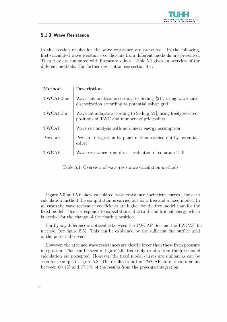
5.1.3 Wave Resistance

In this section results for the wave resistance are presented. In the following,first calculated wave resistance coefficients from different methods are presented.Then they are compared with literature values. Table 5.1 gives an overview of thedifferent methods. For further description see section 4.1.

Method Description

TWCAF Soe Wave cut analysis according to Soding [21], using wave cutsdiscretization according to potential solver grid

TWCAF lin Wave cut anlaysis according to Soding [21], using freely selectedpositions of TWC and numbers of grid points

TWCAF Wave cut analysis with non-linear energy assumption

Pressure Pressure integration by panel method carried out by potentialsolver

TWCAP Wave resistance from direct evaluation of equation 2.19

Table 5.1: Overview of wave resistance calculation methods

Figure 5.5 and 5.6 show calculated wave resistance coefficient curves. For eachcalculation method the computation is carried out for a free and a fixed model. Inall cases the wave resistance coefficients are higher for the free model than for thefixed model. This corresponds to expectations, due to the additional energy whichis needed for the change of the floating position.

Hardly any difference is noticeable between the TWCAF Soe and the TWCAF linmethod (see figure 5.5). This can be explained by the sufficient fine surface gridof the potential solver.

However, the attained wave resistances are clearly lower than these from pressureintegration. This can be seen in figure 5.6. Here only results from the free modelcalculation are presented. However, the fixed model curves are similar, as can beseen for example in figure 5.8. The results from the TWCAF lin method amountbetween 60.4 % and 77.5 % of the results from the pressure integration.

40

0

0.5

1

1.5

2

2.5

3

0.2 0.25 0.3 0.35 0.4 0.45 0.5 0.55

CW·1

03[-

]

Fn [-]

TWCAF Soe (fixed)TWCAF Soe (free)TWCAF lin (fixed)TWCAF lin (free)

Figure 5.5: Wigley hull: Computed wave resistance coefficients

0

0.5

1

1.5

2

2.5

3

3.5

4

0.2 0.25 0.3 0.35 0.4 0.45 0.5 0.55

CW·1

03[-

]

Fn [-]

free modelPressure

TWCAF linTWCAFTWCAP

Figure 5.6: Wigley hull, free model: Computed wave resistance coefficients

41

The consideration of non-linear kinetic wave energy in the TWCAF methodresults to values on the same scale as the pressure integration curve. The maxi-mum deviation between the TWCAF method and the pressure integration resultsamounts 16.2 %. However, the greatest deviations occur for higher Froude num-bers which exceed the range of relevant Froude numbers for merchant ships. Thesame also applies for the results from TWCAP.

Figure 5.7 and 5.8 compare the computed results with different model test mea-surements. Figure 5.9 and 5.10 compare them with calculated results form litera-ture. All values from literature are pooled in envelopes. The separate curves andvalues, which contribute to these envelopes, can be seen in appendix A. For reasonsof clarity, the curve from TWCAF Soe is not shown in the following figures.

0

1

2

3

4

5

6

0.2 0.25 0.3 0.35 0.4 0.45 0.5 0.55

CW·1

03[-

]

Fn [-]

free modelMeasurements

PressureTWCAF lin

TWCAFTWCAP

Figure 5.7: Wigley hull, free model: Comparison with wave resistancemeasurements

42

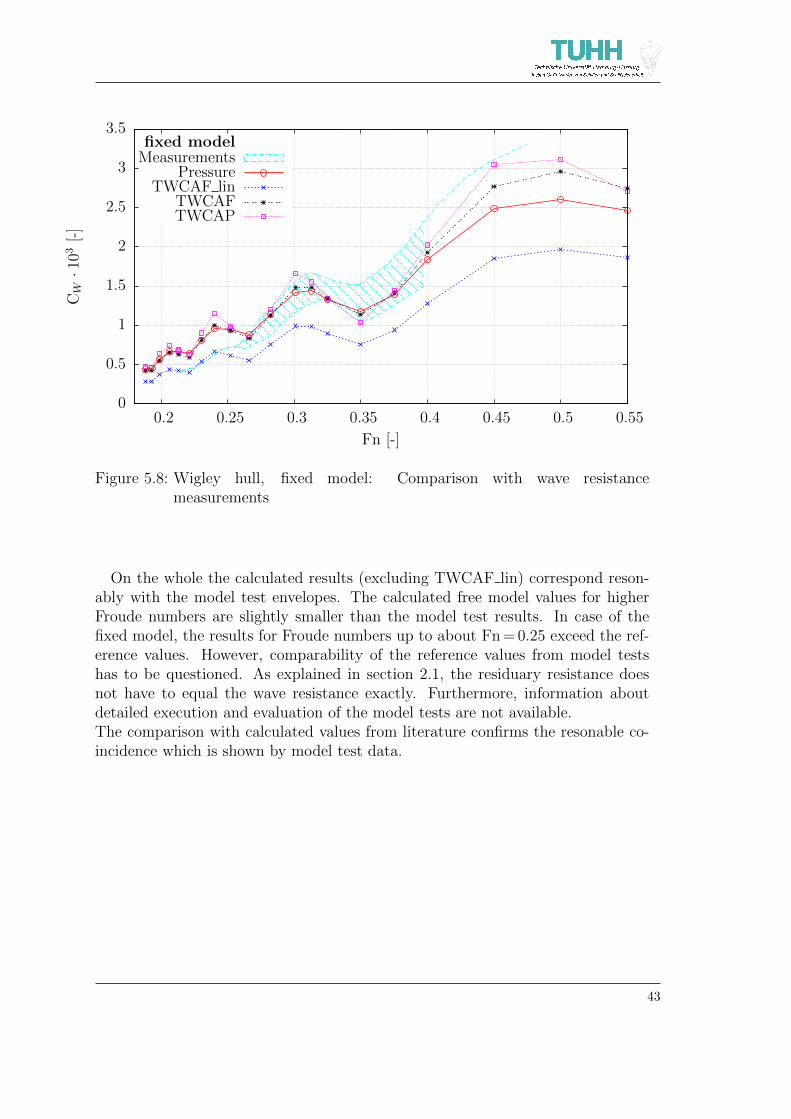
0

0.5

1

1.5

2

2.5

3

3.5

0.2 0.25 0.3 0.35 0.4 0.45 0.5 0.55

CW·1

03[-

]

Fn [-]

fixed modelMeasurements

PressureTWCAF lin

TWCAFTWCAP

Figure 5.8: Wigley hull, fixed model: Comparison with wave resistancemeasurements

On the whole the calculated results (excluding TWCAF lin) correspond reson-ably with the model test envelopes. The calculated free model values for higherFroude numbers are slightly smaller than the model test results. In case of thefixed model, the results for Froude numbers up to about Fn = 0.25 exceed the ref-erence values. However, comparability of the reference values from model testshas to be questioned. As explained in section 2.1, the residuary resistance doesnot have to equal the wave resistance exactly. Furthermore, information aboutdetailed execution and evaluation of the model tests are not available.The comparison with calculated values from literature confirms the resonable co-incidence which is shown by model test data.

43

0

0.5

1

1.5

2

2.5

3

3.5

4

0.2 0.25 0.3 0.35 0.4 0.45 0.5 0.55

CW·1

03[-

]

Fn [-]

free modelCalculations

PressureTWCAF lin

TWCAFTWCAP

Figure 5.9: Wigley hull, free model: Comparison with wave resistance calculations

0

0.5

1

1.5

2

2.5

3

3.5

4

0.2 0.25 0.3 0.35 0.4 0.45 0.5 0.55

CW·1

03[-

]

Fn [-]

fixed modelCalculations

PressureTWCAF lin

TWCAFTWCAP

Figure 5.10: Wigley hull, fixed model: Comparison with wave resistancecalculations

44

5.2 Case 2: RoRo ferry

The developed wave cut analysis is applied for a RoRo ferry. First main character-istics of the ferry are presented. Then the results of the wave resistance calculationsare shown. The calculated results are compared with model test data.

5.2.1 RoRo ferry

The used ship is a 200 m single-screw RoRo ferry. The main dimensions andcharacteristics are shown in table 5.2.

length: Loa 199.800 mLpp 190.292 m

width 26.500 mdesign draught 6.950 mdesign speed 22.5 kncargo capacity 3,831 lane metresaccommodation 12 passengersyear built 2003

Table 5.2: RoRo ferry: Main dimensions

Calculations have been carried out using two different grids for the hull. Theseare shown in figure 5.11 and 5.12.

Figure 5.11: RoRo ferry: Coarse hull grid

45

Figure 5.12: RoRo ferry: Fine hull grid

5.2.2 Wave Resistance

In the following section, wave resistance results are presented. Some variations ofthe grid resolution of the hull (cf. figure 5.11 and 5.12) and the free surface havebeen carried out. As already for the Wigley hull, different calculation methodshave been applied. An overview can be found in table 5.1. The TWCAF Soemethod is not considered here. However, the results are expected to correspondwith the TWCAF lin method.

The considered Froude numbers cover ship’s speeds in the range from 18 to24 kn. The design speed of 22.5 kn corresponds to the Froude number Fn = 0.2614.The results, using fine hull and surface grids, are shown in figure 5.13. As expectedfrom Wigley hull results, the TWCAF lin method provides smaller results thanthe TWCAF method. The linear results amount between 66.4 % and 67.1 % of theresults from the TWCAF method. The values from the TWCAP and the TWCAFmethod are close together. The maximum deviation amounts under 7 %. Thesecharacteristics of the wave cut analysis methods are confirmed as well by the othercalculations for the RoRo ferry.

The Wigley hull curves from TWCAF method are close to the curves frompressure integration. For the RoRo ferry the curves differ. In the range aroundFn = 0.25 the wave resistance coefficients are more or less the same. For smallerFroude numbers the wave cut analysis provides smaller values. At higher Froudenumbers the wave cut analysis results exceed the pressure integration curve.

The calculated wave resistances are compared with model test results. Themodel test curve shows the residuary resistance coefficient. As described in section2.1, the residuary resistance is derived by subtraction of an estimated viscousresistance from the measured total resistance. Thus the residuary resistance is

46

only limitedly suitable for compairison with wave resistances.

However, the deviation is quite high. The wave resistance coefficients fromTWCAF amount only between 18.8 % and 67.7 % of the residuary resistance coef-ficients.

0

0.1

0.2

0.3

0.4

0.5

0.6

0.7

0.8

0.9

1

0.2 0.21 0.22 0.23 0.24 0.25 0.26 0.27 0.28

CR

/CW·1

03[-

]

Fn [-]

CR model testCW pressure

CW TWCAF linCW TWCAFCW TWCAP

Figure 5.13: RoRo ferry: Wave resistance coefficient, fine resolution of hull andfree surface

Normally, grids with a lower resolution are used during hull form design. Thusthe computing time is reduced. Figure 5.14 shows wave resistance coefficient resultsbased on coarse grids for hull and free surface. In contrast to the calculation usingthe finer grids (figure 5.13), the pressure integration results are clearly lower thanthe one from TWCAF method. In addition, the curves, especially these from wavecut methods, are less smooth.

47

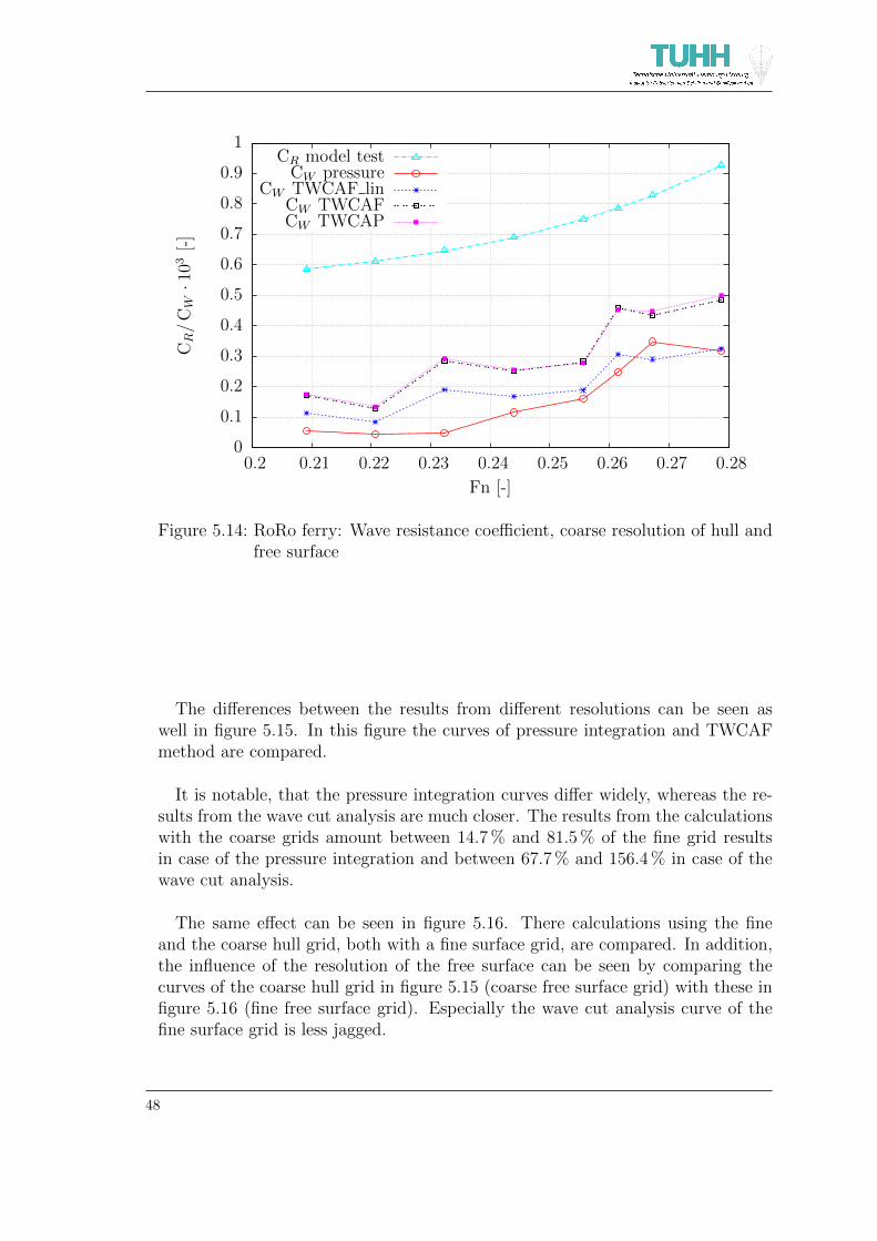
0

0.1

0.2

0.3

0.4

0.5

0.6

0.7

0.8

0.9

1

0.2 0.21 0.22 0.23 0.24 0.25 0.26 0.27 0.28

CR

/CW·1

03[-

]

Fn [-]

CR model testCW pressure

CW TWCAF linCW TWCAFCW TWCAP

Figure 5.14: RoRo ferry: Wave resistance coefficient, coarse resolution of hull andfree surface

The differences between the results from different resolutions can be seen aswell in figure 5.15. In this figure the curves of pressure integration and TWCAFmethod are compared.

It is notable, that the pressure integration curves differ widely, whereas the re-sults from the wave cut analysis are much closer. The results from the calculationswith the coarse grids amount between 14.7 % and 81.5 % of the fine grid resultsin case of the pressure integration and between 67.7 % and 156.4 % in case of thewave cut analysis.

The same effect can be seen in figure 5.16. There calculations using the fineand the coarse hull grid, both with a fine surface grid, are compared. In addition,the influence of the resolution of the free surface can be seen by comparing thecurves of the coarse hull grid in figure 5.15 (coarse free surface grid) with these infigure 5.16 (fine free surface grid). Especially the wave cut analysis curve of thefine surface grid is less jagged.

48

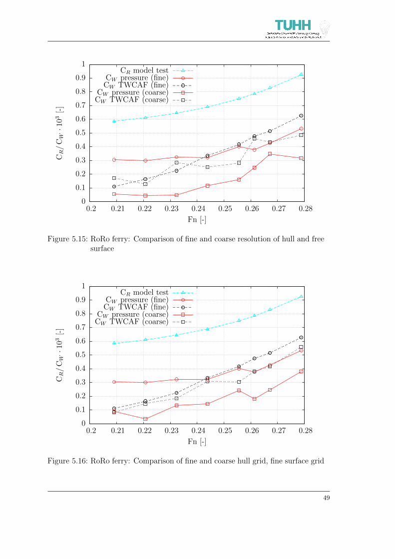
0

0.1

0.2

0.3

0.4

0.5

0.6

0.7

0.8

0.9

1

0.2 0.21 0.22 0.23 0.24 0.25 0.26 0.27 0.28

CR

/CW·1

03[-

]

Fn [-]

CR model testCW pressure (fine)

CW TWCAF (fine)CW pressure (coarse)

CW TWCAF (coarse)

Figure 5.15: RoRo ferry: Comparison of fine and coarse resolution of hull and freesurface

0

0.1

0.2

0.3

0.4

0.5

0.6

0.7

0.8

0.9

1

0.2 0.21 0.22 0.23 0.24 0.25 0.26 0.27 0.28

CR

/CW·1

03[-

]

Fn [-]

CR model testCW pressure (fine)

CW TWCAF (fine)CW pressure (coarse)

CW TWCAF (coarse)

Figure 5.16: RoRo ferry: Comparison of fine and coarse hull grid, fine surface grid

49

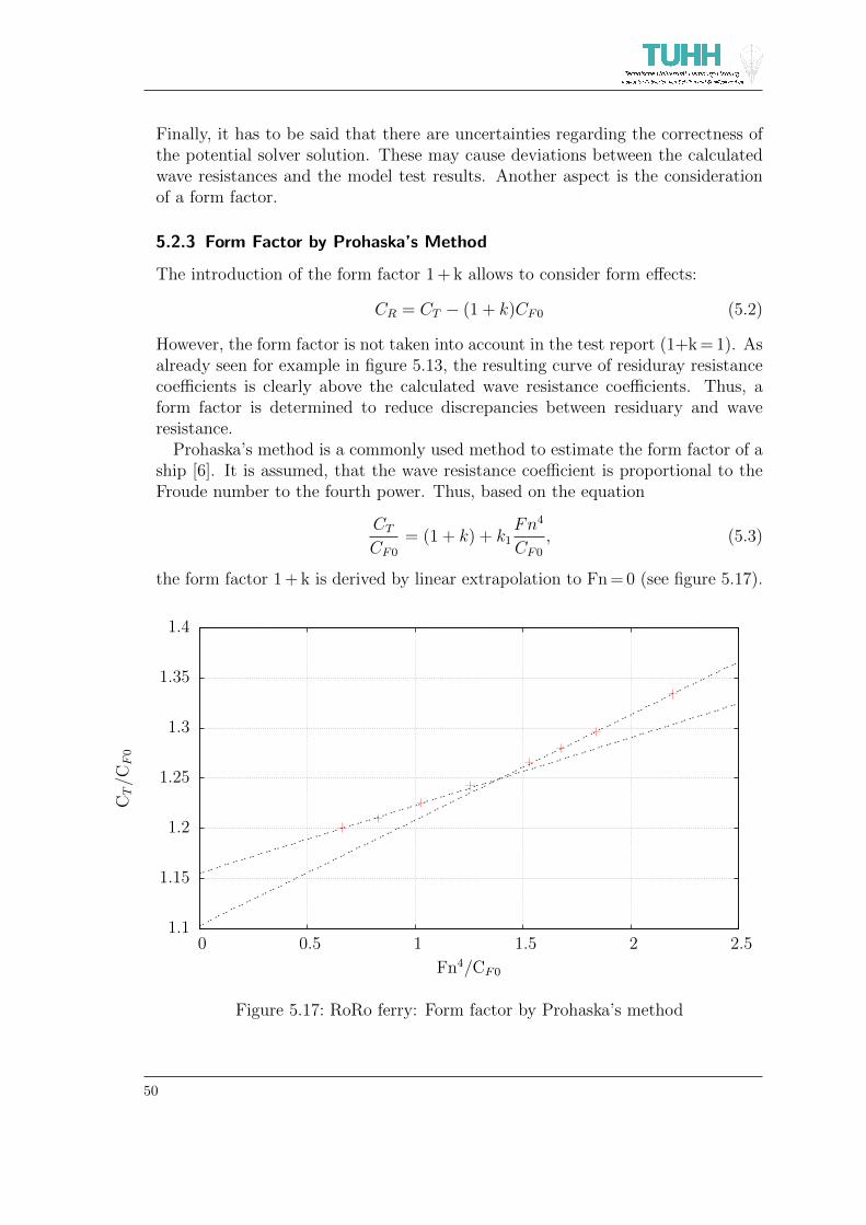
Finally, it has to be said that there are uncertainties regarding the correctness ofthe potential solver solution. These may cause deviations between the calculatedwave resistances and the model test results. Another aspect is the considerationof a form factor.

5.2.3 Form Factor by Prohaska’s Method

The introduction of the form factor 1 + k allows to consider form effects:

CR = CT − (1 + k)CF0 (5.2)

However, the form factor is not taken into account in the test report (1+k = 1). Asalready seen for example in figure 5.13, the resulting curve of residuray resistancecoefficients is clearly above the calculated wave resistance coefficients. Thus, aform factor is determined to reduce discrepancies between residuary and waveresistance.

Prohaska’s method is a commonly used method to estimate the form factor of aship [6]. It is assumed, that the wave resistance coefficient is proportional to theFroude number to the fourth power. Thus, based on the equation

CTCF0

= (1 + k) + k1Fn4

CF0

, (5.3)

the form factor 1 + k is derived by linear extrapolation to Fn = 0 (see figure 5.17).

1.1

1.15

1.2

1.25

1.3

1.35

1.4

0 0.5 1 1.5 2 2.5

CT

/CF0

Fn4/CF0

Figure 5.17: RoRo ferry: Form factor by Prohaska’s method

50

The data points in figure 5.17 are computed with CT and CF0 of the ship model.The straight lines are defined by least square fit. Two form factors are determined,one by using the first three points (Fn = 0.209...0.232) and one by using the lastthree points (Fn = 0.261...0.279).

New residuary resistance coefficient curves are calculated with the form factors(equation 5.2). They are shown in figure 5.18.

0.1

0.2

0.3

0.4

0.5

0.6

0.7

0.8

0.9

1

0.2 0.21 0.22 0.23 0.24 0.25 0.26 0.27 0.28

CR model test1+k = 1.1551+k = 1.103

lin. interpolated kCW TWCAF

Figure 5.18: RoRo ferry: Wave resistance coefficients with form factor

It can be seen, that the correted model test curve with 1+k = 1.155 or 1+k = 1.103matches much better the wave resistance coefficient curve from TWCAF in therange of lower or higher Froude numbers, respectively. Thus, the respective rangesof Froude numbers are in acordance with the considered data points for the de-terminatio of the form factor. This observation fits the assumption that the formfactor of a ship is not constant for different Froude numbers.

Therefore a form factor depending on the Froude number is interpolated linearlybetween 1+k = 1.155 at Fn = 0.209 and 1+k = 1.103 at Fn = 0.279. The resultingresiduary resistance coefficients are close to the values from TWCAF. The devia-tion amounts between 18.6 % and 0.8 %.

51

6 Summary and Conclusion

The goal of this work is the implementation of a reliable wave cut analysis asan alternative to resistance prediction by pressure integration. Therefore, firsta literature research is carried out and relevant publications are presented in areview. As a result of the literature research, the in-house implementation of alinear transverse wave cut analysis (hereinafter called TWCAF lin) correspondswell to state of the art wave cut methods. However, the derived wave resistanceresults are poor compared with pressure integration. Therefore, a new method isdeveloped.

Existing methods are based on a linearized wave resistance formula (equation3.12). The new wave cut analysis is developed from the same expression, butwithout replacing the wave elevation ζ by zero (cf. equation 2.19). There are twodifferent approaches: The first one (hereinafter called TWCAF) uses a Fourieranalysis based flow model. The second one (hereinafter called TWCAP) insertsdirectly the velocity potential derived from a potential solver.

For verification of the wave cut methods and comparison with the pressureintegration, two test cases are used: the ship-like Wigley hull and a RoRo ferry.The application of both developed methods, TWCAF and TWCAP, demonstratessignificant improvements over the method according to Soding and over the othermethods presented in the literature: The decisive enhancement is the considerationof non-linear kinetic wave energy.

Taken this into account, the two validation cases show reasonable results forthe implemented wave cut analysis. The following conclusions are drawn from thewave resistance results of these two test cases.

Wave resistances calculated by TWCAF lin are clearly below reference values.The TWCAF lin results amount only about 67 % of the results from TWCAF.Consequently, the total difference between TWCAF lin and TWCAF method ishigher at higher Froude numbers. This effect corresponds to the increasing waveelevations at higher ship’s speeds.

The results from the TWCAF and the TWCAP method are close together.The TWCAP method is based on a physically correct equation (equation 2.19).Assuming that numerical evaluation errors are small, the results from the TWCAPcan be regarded as a verification of the TWCAF method and the applicability ofthe used flow model. However, the TWCAP method is more time-consuming thanthe wave cut analysis. The time factor between the evaluation of equation 2.19and the TWCAF method scales with three to four per considered x-position.

For a simple hull form like the Wigley hull, the results from pressure integrationcorrespond well to the values form TWCAF. The calculated wave resistances matchwell the measured values from literature. Possibly, further improvement could beachieved by the consideration of a form factor.

52

For a more complicated hull form like the RoRo ferry, the wave resistance valuesand the shape of the resistance curves of the TWCAF method and the pressureintegration differ. Furthermore, the pressure integration is strongly dependent onthe hull and free surface discretization. The TWACF method appears to be morestable.

Especially for ships with a small wave resistance, the resistance prediction ac-cording to Froude’s hypothesis without consideration of a suitable form factor(ITTC-57 recommendations) might be too conservative. The TWCF method givesfor the RoRo ferry only between 18.8 % and 67.7 % of the wave resistance comparedto model test results. However, it can be shown that the introduction of a suitableform factor, depending on the Froude number, reduces the deviation drastically.

For a more automated application of the TWCAF method with less user inter-action, a examination of the conditioning of the linear equation system (equation3.47) is needed. After the calculation of the condition number, the set up could bechanged in case of a poor conditioning. In consequence, the alternative calculationof the Fourier coefficients would not be required anymore for comparison purposes.

An aspect of the flow model, which is not yet investigated, is the impact of theadditional exponential term given by Wehausen (equation 3.17). Behind the ship,the exponential term becomes arbitrarily small with increasing distance. Assumingthat the wave cuts are located sufficient far behind the ship, so far the exponentialterm is not considered for the calculation of the Fourier coefficients.

Since longitudinal wave cut methods are not in the focus of this work, longitudi-nal wave cut methods, especially the implementation of the truncation correction,are not investigated fully exhaustively. However, hopefully, the description in thereview can assists further research.

Finally, it can be said that the TWCAF method provides promising resultsfor the investigated test cases. For further validation and reliability of empiricalvalues, more test cases should be examined.

53

References

[1] E. O. Tuck. The wave resistance formula of j.h. michell (1898) and its signif-icance to recent research in ship hydrodynamics. J. Austral. Math. Soc. Ser.,1989.

[2] J. H. Michell. The wave-resistance of a ship. Philosophical Magazine, 1898.

[3] Hoyte C. Raven and Henk J. Prins. Wave pattern analysis applied to nonlinearship wave calculations. In 13th international Workshop on Water Waves andFloating Bodies, 1998.

[4] Carl-Erik Janson and Daniel Spinney. A comparison of four wave cut anal-ysis methods for wave resistance prediction. Schiffstechnik/Ship TechnologyResearch, (51), 2004.

[5] T. H. Havelock. The wave-making resistance of ships: a theoretical and prac-tical analysis. In Proceedings of the Royal Society, A. Vol. 82, 1909.

[6] Lars Larsson and Hoyte C. Raven. The Principles of Naval ArchitectureSeries: Ship Resistance and Flow. The Society of Naval Architects and MarineEngineers, 2010.

[7] L.W. Ward. Uber die direkte Bestimmung des Wellenwiderstandes ausdem Wellensystem eines Schiffsmodells unter besonderer Berucksichtigung derXY-Methode. Number 2086. Institut fur Schiffbau der Universitat Hamburg,1966.

[8] K. Eggers. Uber die ermittlung des wellenwiderstandes eines schiffsmodellsdurch analyse seines wellensystems. Schiffstechnik Bd. 9 and 10, 1962/1963.

[9] K.W.H. Eggers, S.D. Sharma, and L.W. Ward. An Assessment ofsome Experimental Methods for the Determination of the WavemakingCharacteristics of a Ship Form. Number 184. Institut fur Schiffbau der Uni-versitat Hamburg, 1967.

[10] K. Eggers. Basic theory of wave analysis. Technical report, TU Hamburg-Harburg, 1975.

[11] Toshiaki Mizuno and John. V. Wehausen. Determination of a ship’s waveresistance in a canal from measurements of wave profiles. Technical report,University of Carlifornia Berkeley, 1966.

[12] G.E. Gadd and N. Hogben. The determination of wave resistance from mea-surements of the wave pattern. Technical report, National Physical Labora-tory, Ship Division, 1965.

54

[13] S.D. Sharma. A comparison of the calculated and measured free-wave spec-trum of an inuid in steady motions. In International Seminar on TheoreticalWave-Resistance, Vol. I, 1963.

[14] J.N. Newman. The determination of wave resistance from wave measurementsalong a parallel cut. In International Seminar on Theoretical Wave-Resistance,Vol. I, 1963.

[15] S.W.W. Shor. A fourier transform method for calculating wave-making resis-tance from wave height on a line parallel to a ship’s track. In InternationalSeminar on Theoretical Wave-Resistance, Vol. II, 1963.

[16] Pao C. Pien and Wilburn L. Moore. Theoretical and experimental studyon wave-making resistance of ships. In International Seminar on TheoreticalWave-Resistance, Vol. I, 1963.

[17] Hisashi Kajitani. Wave resistance obtained from photogrammetical analysis ofthe wave pattern. In International Seminar on Theoretical Wave-Resistance,Vol. I, 1963.

[18] G.E. Gadd and N. Hogben. An appraisal of the ship resistance problem inthe light of measurements of the wave pattern. Technical report, NationalPhysical Laboratory, Ship Division, 1962.

[19] N. Hogben. The computing of wave resistance from a wave pattern by a matrixmethod. Technical report, National Physical Laboratory, Ship Division, 1964.

[20] John V. Wehausen. The Wave Resistance of Ships. Department of NavalArchitecture, University of Carlifornia Berkeley, 1973.

[21] H. Soding. Far-field ship waves. Ship Technology Research Vol. 53, 2006.

[22] H. Soding. Widerstand aus dem wellenbild: Programm kelw. Technical report,TU Hamburg-Harburg, 2001.

[23] Lawrence W. Ward. The xy method of determination of ship wave re-sistance from the wave pattern. In International Seminar on TheoreticalWave-Resistance, Vol. I, 1963.

[24] T. H. Havelock. The calculation of wave resistance. In Proceedings of theRoyal Society, A. Vol. 82, 1934.

[25] F.C. Michelsen and S.B.S. Uberoi. A study of wave resistance characteristicsthrough the analysis of wave height and slope along a longitudinal track.Technical report, Hydro- and Aerodynamics Laboratory - Denmark, 1971.

55

[26] Justus Heimann. CFD Based Optimization of the Wave-MakingCharacteristics of Ship Hulls. PhD thesis, Technische Universitat Berlin, 2005.

[27] K. Eggers. On the determination of the wave resistance of a ship modelby an analysis of its wave system. In International Seminar on TheoreticalWave-Resistance, Vol. III, 1963.

[28] Justus Heimann. Application of wave pattern analysis in a cfd basedhull design process. In 3rd Int. Numerical Towing Tank Symposium 2000(NUTTS’00), 2000.

[29] Heinrich Soding. personal correspondence.

[30] Moustafa Abdel-Maksoud. Schiffsdynamik. lecture notes, TU Hamburg-Harburg.

[31] Johannes Will, 2014. unpublished.

[32] Gerhard Jensen. Berechnung der stationaren potentialstromung um ein schiffunter berucksichtigung der nichtlinearen randbedingungen an der wasserober-flache. Technical report, TU Hamburg-Harburg, 1988.

[33] Johannes Will. personal correspondence.

[34] RINA. An Investigation into the Resistance Components of High SpeedDisplacement Catamarans, 1991.

[35] Zaojian Zou. Berechnung der potentialstromung um einen schrag fahrendenschiffsrumpf auf tiefem und flachem wasser. Technical report, TU Hamburg-Harburg, 1994.

[36] Michael Hughes and Volker Bertram. A higher-order panel method for 3-dfree surface flows. Technical report, Institut fur Schiffbau, 1995.

[37] Hun Chol Kim and Finn C. Michelsen. Experimental wave component analysisas applied to ship wave systems. Technical report, The University of Michigan,1966.

[38] Me 241 marine hydrodynamics, 2009. lecture notes, UC Berkely.

[39] Volker Bertram. Numerische schiffshydrodynamik in der praxis. Technicalreport, TU Hamburg-Harburg, 1994.

[40] Sakir Bal. Prediction of wave pattern and wave resistance of surface piercingbodies by a boundary element method. Int. J. Numer. Meth. Fluids, 2008.

[41] Louis Landweber. Wigley parabolic hull group discussion. In Proceedings ofthe Workshop on Ship Wave-Resistance Computations, Vol. I, 1979.

56

[42] Xujian Lv, Xiaoguang Wu, Jianglong Sun, and Haiwen Tu. Trim optimiza-tion of ship by a potential-based panel method. Advances in MechanicalEngineering, 2013. Huazhong University of Science and Technology.

[43] Nakos and Sclavounos. Kelvin wakes and wave resistance of cruiser- andtransom-stern ships. Journal of Ship Research, 1994.

57

A Wave Resistances of Wigley Hull from Literature

0

1

2

3

4

5

6

0.2 0.25 0.3 0.35 0.4 0.45 0.5 0.55

CW·1

03[-

]

Fn [-]

free modelEnvelope of measurements

Kajitani 1987 [39]

RINA [34]

Wave pattern RINA [34]

WPHGD [41]

Figure A.1: Wigley hull, free model: Measured wave resistance data

The envelope of measurements does not consider the data ”wave pattern RINA”.The reason is, that the measured wave pattern has to be evaluated by wave cutanalysis to determine wave resistances.

The envelope of experimental data taken from the Wigley parabolic hull groupdiscussion (WPHGD) [41] contains the following data:

- residual resistance (Lackenby, 1965)

- pressure resistance (Lackenby, 1965)

- thin ship theory (Lackenby, 1965)

- wave resistance (transverse cut, Gadd & Hogben, 1965)

- residual resistance, 8 m model (Mitsubishi Nagasaki experimental tank)

- residual resistance, 5 m model (Mitsubishi Nagasaki experimental tank)

- residual resistance (IHI ship model basin – free to sink & trim)

59

Fn 0.180 0.200 0.220 0.240 0.266Shearer CW = Cr− (CV )wake survey 0.29 0.45 0.65 0.85 0.94

and Cross Cr 0.39 0.54 0.73 0.92 1.04Univ. of Tokyo (trim restrained) 0.38 0.48 0.62 0.88 1.01Univ. of Tokyo (trim restrained) 0.25 0.43 0.54 0.79 0.97Ship Research Institute -0.03 0.26 0.47 0.87 0.97Ship Research Institute 0.17 0.34 0.34 0.76 0.98Mitsubishi-Nagasaki 0.34 0.48 0.70 0.96 1.06Mitsubishi-Nagasaki 0.17 0.51 0.64 0.96 1.03Ishihawajima-Harima 0.26 0.36 0.52 0.84 0.95

Fn 0.313 0.350 0.402 0.452 0.482Shearer CW = Cr− (CV )wake survey 1.80 1.62 2.80 4.10 4.46

and Cross Cr 1.91 1.82 2.87 4.43 4.78Univ. of Tokyo (trim restrained) 1.88 1.79 2.96 – –Univ. of Tokyo (trim restrained) 1.83 1.72 2.87 – –Ship Research Institute 1.77 1.73 2.84 – –Ship Research Institute 1.85 1.77 – – –Mitsubishi-Nagasaki 2.01 1.85 3.09 – –Mitsubishi-Nagasaki 1.94 1.83 3.31 – –Ishihawajima-Harima 1.91 – – – –

Table A.1: Wigley hull, free model: Experimental Data WPHGD [41]

60

0

0.5

1

1.5

2

2.5

3

3.5

0.2 0.25 0.3 0.35 0.4 0.45 0.5 0.55

CW·1

03[-

]

Fn [-]

fixed modelEnvelope of measurements

ITTC 1984 [43]

Huanzhong Uni. 2013 [42]

Figure A.2: Wigley hull, fixed model: Measured wave resistance data

0

1

2

3

4

5

6

0.2 0.25 0.3 0.35 0.4 0.45 0.5 0.55

CW·1

03[-

]

Fn [-]

free modelEnvelope of calculationsWave pattern RINA [34]

Calculation Zou [35]

Panel-Method Jensen [32]

Panel-Method Bertram [36]

Figure A.3: Wigley hull, free model: Calculated wave resistance data

The envelope of calculations does not consider the data ”wave pattern RINA”. The

61

reason is that these calculated values are based on measured wave pattern.

Fn 0.20 0.22 0.24 0.25 0.267 0.30 0.316 0.35 0.40CW · 103

linear0.744 0.760 1.025 1.036 1.056 1.694 1.711 1.237 2.243

CW · 103

non-linear0.642 0.590 1.080 1.035 0.978 1.778 1.859 1.554 2.614

Table A.2: Wigley hull, free model: Calculation Zou [35]

0

0.5

1

1.5

2

2.5

3

3.5

4

0.2 0.25 0.3 0.35 0.4 0.45 0.5 0.55

CW·1

03[-

]

Fn [-]

fixed modelEnvelope of calculations

Thin-Ship Theory Bertram [39]

Calculation Bal (TWC) [40]

Huanzhong Uni. 2013 [42]

Linear pressure int. NakosNear-field pressure int. Nakos

Far-field WCA Nakos [43]

Figure A.4: Wigley hull, free model: Calculated wave resistance data

62

B Wave Resistance Results of Wigley Hull

Fn TWCAF Soe TWCAF lin TWCAF TWCAP pressure0.188 0.289 0.288 0.432 0.481 0.4770.193 0.288 0.287 0.430 0.466 0.4600.199 0.371 0.378 0.567 0.655 0.5800.206 0.450 0.449 0.673 0.764 0.6820.213 0.436 0.437 0.655 0.713 0.6710.221 0.409 0.407 0.610 0.639 0.6620.230 0.537 0.547 0.820 0.911 0.8090.240 0.683 0.685 1.028 1.185 1.0140.252 0.647 0.648 0.973 1.031 0.9620.266 0.552 0.559 0.833 0.857 0.8740.282 0.820 0.816 1.224 1.307 1.2300.301 1.077 1.086 1.629 1.828 1.5180.313 1.074 1.611 1.688 1.5190.325 1.000 0.998 1.497 1.503 1.4780.350 0.870 0.872 1.308 1.190 1.3050.375 1.054 1.068 1.603 1.652 1.5840.400 1.522 1.526 2.289 2.419 2.1580.450 2.346 2.334 3.501 3.868 3.0120.500 2.503 2.502 3.753 3.972 3.2490.550 2.294 2.301 3.451 3.418 3.004

Table B.1: Wigley hull, free model: Wave resistance coefficients

63

Fn TWCAF Soe TWCAF lin TWCAF TWCAP pressure0.188 0.287 0.286 0.429 0.478 0.4430.193 0.285 0.284 0.426 0.461 0.4510.199 0.364 0.370 0.556 0.639 0.5630.206 0.439 0.438 0.657 0.744 0.6710.213 0.420 0.630 0.685 0.6620.221 0.398 0.396 0.595 0.623 0.6370.230 0.533 0.542 0.813 0.903 0.8070.240 0.662 0.664 0.996 1.147 0.9650.252 0.617 0.619 0.929 0.983 0.9490.266 0.548 0.552 0.828 0.846 0.8790.282 0.755 0.752 1.128 1.201 1.1430.301 0.983 0.991 1.486 1.665 1.4140.313 0.989 1.484 1.552 1.4390.325 0.894 0.891 1.337 1.339 1.3260.350 0.756 0.758 1.137 1.033 1.1800.375 0.928 1.940 1.411 1.441 1.3960.400 1.278 1.282 1.922 2.022 1.8360.450 1.857 1.848 2.772 3.051 2.4910.500 1.967 1.970 2.955 3.116 2.6060.550 1.819 1.868 2.738 2.703 2.462

Table B.2: Wigley hull, fixed model: Wave resistance coefficients

C Wave Resistance Results of RoRo ferry

U [kn] Fn [–] CR [–]18.0 0.209 0.58619.0 0.221 0.61120.0 0.232 0.64621.0 0.244 0.69022.0 0.256 0.74922.5 0.261 0.78623.0 0.267 0.82924.0 0.279 0.926

Table C.1: RoRo ferry: Wave resistance coefficients from model test

64

Fn TWCAF lin TWCAF TWCAP pressure0.209 0.073 0.110 0.109 0.3050.221 0.110 0.164 0.156 0.3000.232 0.150 0.225 0.215 0.3240.244 0.223 0.335 0.314 0.3230.256 0.278 0.418 0.413 0.4010.261 0.318 0.477 0.464 0.3780.267 0.343 0.515 0.516 0.4270.279 0.418 0.627 0.644 0.533

Table C.2: RoRo ferry: Wave resistance coefficients, fine resolution of hull and freesurface

Fn TWCAF lin TWCAF TWCAP pressure0.209 0.115 0.172 0.175 0.0560.221 0.086 0.129 0.134 0.0460.232 0.191 0.286 0.293 0.0480.244 0.168 0.252 0.256 0.1160.256 0.189 0.283 0.279 0.1600.261 0.307 0.461 0.453 0.2480.267 0.290 0.435 0.449 0.3480.279 0.324 0.486 0.500 0.317

Table C.3: RoRo ferry: Wave resistance coefficients, coarse resolution of hull andfree surface

Fn TWCAF lin TWCAF TWCAP pressure0.209 0.054 0.082 0.084 0.0890.221 0.098 0.146 0.144 0.0360.232 0.123 0.185 0.182 0.1320.244 0.207 0.310 0.298 0.1430.256 0.204 0.306 0.296 0.2420.261 0.255 0.382 0.368 0.1800.267 0.278 0.417 0.416 0.2450.279 0.373 0.559 0.581 0.382

Table C.4: RoRo ferry: Wave resistance coefficients, coarse hull grid, fine surfacegrid

65