ETH Library Schramm-Loewner Evolution and long-range correlated systems Doctoral Thesis Author(s): Posé, Nicolas Publication date: 2015 Permanent link: https://doi.org/10.3929/ethz-a-010552449 Rights / license: In Copyright - Non-Commercial Use Permitted This page was generated automatically upon download from the ETH Zurich Research Collection . For more information, please consult the Terms of use .

Welcome message from author
This document is posted to help you gain knowledge. Please leave a comment to let me know what you think about it! Share it to your friends and learn new things together.
Transcript

ETH Library
Schramm-Loewner Evolution andlong-range correlated systems
Doctoral Thesis
Author(s):Posé, Nicolas
Publication date:2015
Permanent link:https://doi.org/10.3929/ethz-a-010552449
Rights / license:In Copyright - Non-Commercial Use Permitted
This page was generated automatically upon download from the ETH Zurich Research Collection.For more information, please consult the Terms of use.
Diss. ETH No. 22774
Schramm-Loewner Evolutionand long-range correlated
systems
A thesis submitted to attain the degree of
DOCTOR OF SCIENCES of ETH ZURICH
(Dr. sc. ETH Zurich)
presented by
Nicolas Pose
MSc ETH Physics,
Ingenieur diplome de l’Ecole Polytechnique
born on 24.10.1987
citizen of France
accepted on the recommendation of
Prof. Dr. Hans J. Herrmann, examiner
Prof. Dr. Alexander K. Hartmann, co-examiner
2015


Acknowledgment
I have to thank my supervisor Professor Hans J. Herrmann for allowing me
to work on a challenging topic in an inspiring environment.
I also would like to thank Professor Alexander K. Hartmann for having ac-
cepted to review my work.
Thanks are also due to my collaborators, with whom I worked on the different
projects presented in this thesis. First I would like to thank Professor Nuno
A. M. Araujo for the numerous discussions we had, the ideas we discussed,
his knowledge and experience he shared. I also would like to thank Dr. Ken
J. Schrenk for the work we started together and his help. I also want to
thank Dr. Miller Mendoza for the work we did together on graphene, the
inspiring discussions we had and his advices. I also thank my collaborators
Ilario Giordanelli, Laurens V. M. van Kessenich and Julian J. Kranz.
I am also grateful to my coworkers, Dominik and Trivik with whom I shared
the office in the past two years, Miller, Nuno, Julian, Vitor, Ilias, Farhang,
Roman, Fabrizio, Jan, Oliver, Ryuta, Sergio, Jens-Daniel, Ilario, Robin, Gau-
tam and the whole Comphys-Group for the nice time I spent with them.
I am also grateful to Professor Denis Bernard and Professor Wendelin Werner
for helpfull discussions and to all my teachers at the Ecole Polytechnique in
Paris and ETH Zurich for their enthousiasm in transmitting their knowledge.
Last but not least, I would like to thank my relatives, especially my parents,
for their unconditionnal help, Sara for her support during these years, and all
my friends not only in Zurich but wherever they might be now for spending
so many nice moments together.
3
4
Contents
1 Introduction 1
2 Schramm-Loewner Evolution theory 7
2.1 Conformal transformations and holomorphic functions . . . . . 9
2.2 The Riemann mapping theorem and its consequences . . . . . 10
2.3 Half-plane capacity parametrization . . . . . . . . . . . . . . . 12
2.4 The Loewner differential Equation and the driving function . . 13
2.5 Schramm-Loewner Evolution theory . . . . . . . . . . . . . . . 16
2.6 Mapping of curves generated in a rectangle into the upper-half
plane . . . . . . . . . . . . . . . . . . . . . . . . . . . . . . . . 22
2.7 Numerical tests of Schramm-Loewner Evolution . . . . . . . . 23
2.7.1 The fractal dimension . . . . . . . . . . . . . . . . . . 25
2.7.2 The winding angle . . . . . . . . . . . . . . . . . . . . 25
2.7.3 The left-passage probability . . . . . . . . . . . . . . . 26
2.7.4 The direct SLE algorithm . . . . . . . . . . . . . . . . 29
2.8 Known results in SLE . . . . . . . . . . . . . . . . . . . . . . 32
3 Shortest path in percolation and Schramm-Loewner Evolu-
tion 35
3.1 Introduction . . . . . . . . . . . . . . . . . . . . . . . . . . . . 36
3.2 Method . . . . . . . . . . . . . . . . . . . . . . . . . . . . . . 38
3.3 Winding angle method . . . . . . . . . . . . . . . . . . . . . . 39
3.4 Left passage probability method . . . . . . . . . . . . . . . . . 39
3.5 Direct SLE method . . . . . . . . . . . . . . . . . . . . . . . . 41
3.5.1 In chordal space . . . . . . . . . . . . . . . . . . . . . . 41
i
3.5.2 In dipolar space . . . . . . . . . . . . . . . . . . . . . . 43
3.6 Final Remarks . . . . . . . . . . . . . . . . . . . . . . . . . . . 47
4 Long-range correlated landscapes and correlated percolation 49
4.1 Correlated percolation . . . . . . . . . . . . . . . . . . . . . . 50
4.2 The Hurst exponent of long-range correlated landscapes . . . . 52
4.3 The Fourier Filtering Method for correlated landscapes . . . . 53
4.4 Correlated surfaces, Fourier Filtering Method and fractional
Gaussian fields . . . . . . . . . . . . . . . . . . . . . . . . . . 57
5 Long-range correlated percolation 63
5.1 Introduction . . . . . . . . . . . . . . . . . . . . . . . . . . . . 64
5.2 Correlated percolation and the extended Harris criterion . . . 65
5.3 Percolation threshold . . . . . . . . . . . . . . . . . . . . . . . 67
5.4 Maximum cluster size and cluster size distribution . . . . . . . 69
5.5 Cluster perimeters . . . . . . . . . . . . . . . . . . . . . . . . 74
5.6 Transport properties: shortest path, backbone and cluster
conductivity . . . . . . . . . . . . . . . . . . . . . . . . . . . . 79
5.7 Final remarks . . . . . . . . . . . . . . . . . . . . . . . . . . . 86
6 Schramm-Loewner Evolution on long-range correlated land-
scapes 89
6.1 Introduction . . . . . . . . . . . . . . . . . . . . . . . . . . . . 90
6.2 Isoheight lines on correlated landscapes with negative Hurst
exponent . . . . . . . . . . . . . . . . . . . . . . . . . . . . . . 91
6.2.1 SLE and fractal dimension . . . . . . . . . . . . . . . . 92
6.2.2 Winding angle . . . . . . . . . . . . . . . . . . . . . . . 92
6.2.3 Left Passage Probability . . . . . . . . . . . . . . . . . 94
6.2.4 Direct SLE . . . . . . . . . . . . . . . . . . . . . . . . 96
6.3 Isoheight lines on correlated landscapes with positive Hurst
exponent . . . . . . . . . . . . . . . . . . . . . . . . . . . . . . 98
6.3.1 Winding angle . . . . . . . . . . . . . . . . . . . . . . . 98
6.3.2 Left-Passage probability . . . . . . . . . . . . . . . . . 98
6.3.3 Direct SLE method . . . . . . . . . . . . . . . . . . . . 98
ii
6.4 Markovian properties of the driving functions . . . . . . . . . 103
6.5 Other critical curves . . . . . . . . . . . . . . . . . . . . . . . 103
6.5.1 Winding angle measurements for the shortest path and
the watersheds . . . . . . . . . . . . . . . . . . . . . . 105
6.5.2 Direct SLE test for the shortest path . . . . . . . . . . 108
6.5.3 Direct SLE and left-passage probability for watersheds 110
6.6 Conclusion . . . . . . . . . . . . . . . . . . . . . . . . . . . . . 114
7 Conformal Invariance in Graphene 119
7.1 Introduction . . . . . . . . . . . . . . . . . . . . . . . . . . . . 120
7.2 Methodology . . . . . . . . . . . . . . . . . . . . . . . . . . . 122
7.3 Scale invariance in graphene . . . . . . . . . . . . . . . . . . . 123
7.4 Conformal invariance and SLE properties in graphene . . . . . 126
7.5 Difference between graphene sheets and Gaussian random sur-
faces . . . . . . . . . . . . . . . . . . . . . . . . . . . . . . . . 131
7.6 Conclusion . . . . . . . . . . . . . . . . . . . . . . . . . . . . . 132
8 Discussion and Outlook 135
References 139
iii

iv

List of Figures
1.1 Loop-Erased Random Walk Discreate Loop-Erased Ran-
dom Walk in the upper half-plane. It has been generated us-
ing the transition probabilities defined in Ref. [1] for a random
walk half-plane excursion. The discreate upper half-plane is
defined as Z+ iZ+ = {j + ik, j ∈ Z, k ∈ Z+}. . . . . . . . . . . 4
1.2 Percolation Percolation interface generated on a triangular
lattice in a rectangle with Dirichlet boundary conditions, i.e.
with zero value (red sites) on half of the border and one (blue
sites) on the other half. The interface, displayed as a black
solid line, is defined such that the interface path starting from
the bottom line has always a red site on its left and a blue site
on its right. . . . . . . . . . . . . . . . . . . . . . . . . . . . . 5
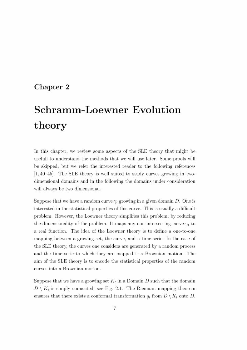
2.1 A growing curve (γt)t≥0 in the domainD, in this case the upper
half-plane. The hull Kt is here defined as the curve taken till
time t, and D \Kt is the domain D from which one substracts
Kt. . . . . . . . . . . . . . . . . . . . . . . . . . . . . . . . . . 8
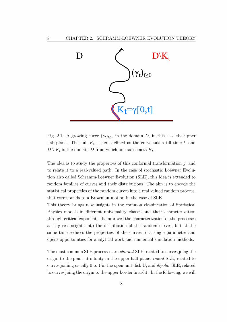
2.2 Conformal mapping of the upper half plane H = {z ∈C, Im(z) > 0} into the unit disk {z ∈ C, |z| < 1}, using
f(z) = z−iz+i
. . . . . . . . . . . . . . . . . . . . . . . . . . . . . 10
2.3 Mapping gt : H \ Kt → H. The hull is shown in blue and is
mapped to the real line by gt. . . . . . . . . . . . . . . . . . . 12
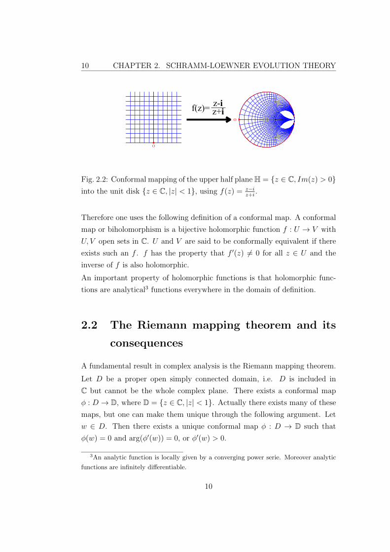
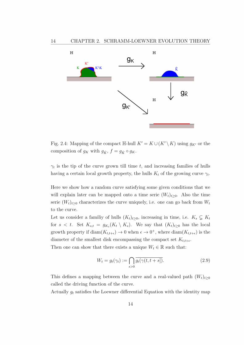
2.4 Mapping of the compact H-hull K ′ = K ∪ (K ′ \K) using gK′
or the composition of gK with gK , f = gK ◦ gK . . . . . . . . . 14
v

2.5 For 0 ≤ κ ≤ 4, the curves are simple. For 4 < κ < 8 they are
self touching and for κ ≥ 8 they are space filling . . . . . . . . 17
2.6 The two probability measures in the domains D and D \ γ[a,c].
If the Domain Markov Property is satisfied, these two proba-
bilities are equal. . . . . . . . . . . . . . . . . . . . . . . . . . 20
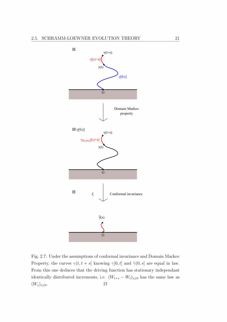
2.7 Under the assumptions of conformal invariance and Domain
Markov Property, the curves γ(t, t + s] knowing γ[0, t] and
γ(0, s] are equal in law. From this one deduces that the driv-
ing function has stationary independant identically distributed
increments, i.e. (Wt+s −Wt)s≥0 has the same law as (Ws)s≥0. . 21
2.8 Mapping from a rectangle into the upper half plane
Rectangle mapped to the upper half-plane. (a) Rectangle of
aspect ratio 1 and (b) mapped points into the upper half-
plane. (c) Rectangle of aspect ratio 2 and (d) mapped points
into the upper half-plane. (e) Rectangle of aspect ratio 4 and
(f) mapped points into the upper half-plane. . . . . . . . . . . 24
2.9 (Winding angle) The winding angle is defined iteratively,
as the sum of the turning angles αi between two consecutive
segments (zi−1, zi) and (zi, zi+1). . . . . . . . . . . . . . . . . . 27
2.10 (Left passage) Curve separating the space into the points
belonging to the right side of the curve (space marked in grey)
and points belonging to the left side of the curve (space left
blank). . . . . . . . . . . . . . . . . . . . . . . . . . . . . . . . 28
2.11 (Left passage probability) Probability of a point belonging
the right side of the curve dependant on the angle φ. The left-
passage probability is independant on the value of the radius
R of the point z ∈ H. . . . . . . . . . . . . . . . . . . . . . . . 29
2.12 Iteration of the conformal maps gti : H \ gti−1◦ . . . ◦
g1(γ([ti−1, ti])) → H and extraction of the underlying driving
function. . . . . . . . . . . . . . . . . . . . . . . . . . . . . . . 30
2.13 Approximation made in the ’vertical’ slit map algorithm . . . 31
vi

3.1 A spanning cluster on the triangular lattice in a strip of ver-
tical size Ly = 512. The shortest path is in red and all the
other sites belonging to the spanning cluster are in blue. . . . 37
3.2 Variance of the winding angle against the lattice size Ly. The
analysis has been done for Ly ranging from 16 to 16384. The
statistics are computed over 104 samples. The error bars are
smaller than the symbol size. By fitting the results with
Eq. (2.25), one gets κwinding = 1.046± 0.004. In the inset, the
probability distribution of the winding angle along the curve
is compared to the predicted Gaussian distribution, drawn in
green, of variance κ4
ln(Ly) with κ = 1.046 and Ly = 16384. . . 40
3.3 Left passage probability test. (a) Weighted mean square de-
viation Q(κ) as a function of κ, for Ly = 16384. The vertical
blue line corresponds the minimum of Q(κ), and the green
vertical line is a guide to the eye at κ = κfract. The minimum
of the mean square deviation is at κLPP = 1.038± 0.019. The
light blue area corresponds to the error bar on the value of
κLPP . (b) Computed left passage probability as a function of
φ/π for R ∈ [0.70, 0.75] and κ = 1.038. The blue line is a
guide to the eye of Schramm’s formula (2.26) for κ = 1.038. . . 42
3.4 Driving function computed using the slit map algorithm. (a)
Mean square deviation of the driving function 〈ξ2t 〉 as a func-
tion of the Loewner time t. The diffusion coefficient κ is given
by the slope of the curve. In the inset we see the local slope
κdSLE(t). The thick green line is a guide to the eye corre-
sponding to κdSLE = 0.92. (b) Plot of the correlation c(t, τ)
given by Eq. (3.1), and averaged over 50 time steps. The
averaged value is denoted c(τ). In the inset are shown the
probability distributions of the driving function for three dif-
ferent Loewner times t1 = 1.2 × 10⁻³, t2 = 3.7 × 10⁻³ and
t3 = 9.95 × 10⁻³. The solid lines are guides to the eye of the
form P (ξt) = 1√2πκti
exp(− ξ2t
2κti
), for i = 1, 2, 3. . . . . . . . . . 44
vii
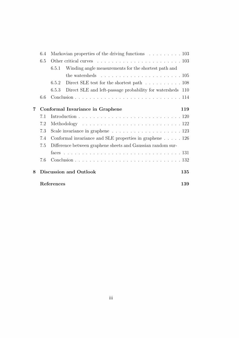
3.5 Driving function computed using the dipolar slit map given
by Eq. (3.3), for Ly = 16384. The mean square deviation of
the driving function 〈ξ2t 〉− 〈ξt〉2 is plotted as a function of the
Loewner time t. The diffusion coefficient κ is given by the
slope of the curve. . . . . . . . . . . . . . . . . . . . . . . . . . 46
4.1 A random landscape and its percolation clusters. In blue are
the empty sites and in brown the occupied ones. The sites
in green belong to the percolating cluster. The paths in red
represent the left and right accessible perimeters and the paths
in yellow the one site wide fjords. . . . . . . . . . . . . . . . . 51
4.2 Random landscapes generated with the Fourier filtering
method for different values of the Hurst exponent: (a) H =
−1, (b) H = −0.5, (c) H = 0, and (d) H = 0.5. . . . . . . . . 55
4.3 Properites of the Fourier transform of one random landscape of
Hurst exponentH = −0.5 generated with the Fourier Filtering
Method. (a) Power spectrum Sq = |h(q)|2 as a function of |q|,where h is the Fourier transform of the surface h. The red line
is a guide to the eye of the form |q|−βc with βc = 2(H + 1).
(b) Phase φ = arg(h(q)) as a function of q = (qx, qy). . . . . . 56
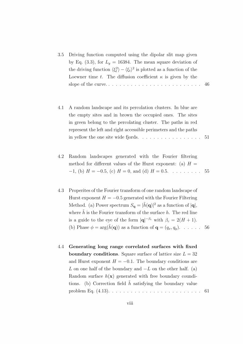
4.4 Generating long range correlated surfaces with fixed
boundary conditions. Square surface of lattice size L = 32
and Hurst exponent H = −0.1. The boundary conditions are
L on one half of the boundary and −L on the other half. (a)
Random surface h(x) generated with free boundary coundi-
tions. (b) Correction field h satisfying the boundary value
problem Eq. (4.13). . . . . . . . . . . . . . . . . . . . . . . . . 61
viii
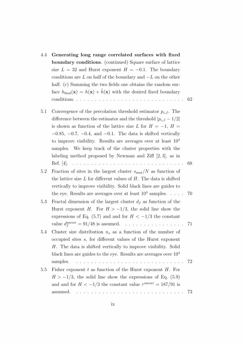
4.4 Generating long range correlated surfaces with fixed
boundary conditions. (continued) Square surface of lattice
size L = 32 and Hurst exponent H = −0.1. The boundary
conditions are L on half of the boundary and −L on the other
half. (c) Summing the two fields one obtains the random sur-
face hfinal(x) = h(x) + h(x) with the desired fixed boundary
conditions. . . . . . . . . . . . . . . . . . . . . . . . . . . . . . 62
5.1 Convergence of the percolation threshold estimator pc,J . The
difference between the estimator and the threshold |pc,J − 1/2|is shown as function of the lattice size L for H = −1, H =
−0.85, −0.7, −0.4, and −0.1. The data is shifted vertically
to improve visibility. Results are averages over at least 104
samples. We keep track of the cluster properties with the
labeling method proposed by Newman and Ziff [2, 3], as in
Ref. [4]. . . . . . . . . . . . . . . . . . . . . . . . . . . . . . . 68
5.2 Fraction of sites in the largest cluster smax/N as function of
the lattice size L for different values of H. The data is shifted
vertically to improve visibility. Solid black lines are guides to
the eye. Results are averages over at least 104 samples. . . . . 70
5.3 Fractal dimension of the largest cluster df as function of the
Hurst exponent H. For H > −1/3, the solid line show the
expressions of Eq. (5.7) and and for H < −1/3 the constant
value duncorrf = 91/48 is assumed. . . . . . . . . . . . . . . . . 71
5.4 Cluster size distribution ns as a function of the number of
occupied sites s, for different values of the Hurst exponent
H. The data is shifted vertically to improve visibility. Solid
black lines are guides to the eye. Results are averages over 104
samples. . . . . . . . . . . . . . . . . . . . . . . . . . . . . . 72
5.5 Fisher exponent t as function of the Hurst exponent H. For
H > −1/3, the solid line show the expressions of Eq. (5.9)
and and for H < −1/3 the constant value τuncorr = 187/91 is
assumed. . . . . . . . . . . . . . . . . . . . . . . . . . . . . . 73
ix
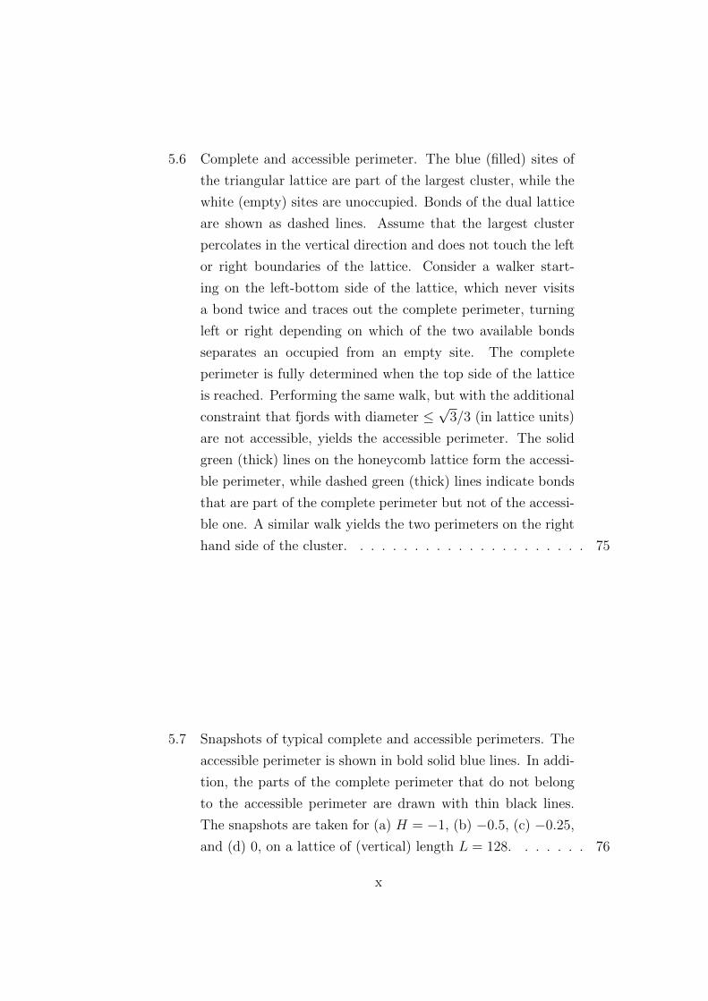
5.6 Complete and accessible perimeter. The blue (filled) sites of
the triangular lattice are part of the largest cluster, while the
white (empty) sites are unoccupied. Bonds of the dual lattice
are shown as dashed lines. Assume that the largest cluster
percolates in the vertical direction and does not touch the left
or right boundaries of the lattice. Consider a walker start-
ing on the left-bottom side of the lattice, which never visits
a bond twice and traces out the complete perimeter, turning
left or right depending on which of the two available bonds
separates an occupied from an empty site. The complete
perimeter is fully determined when the top side of the lattice
is reached. Performing the same walk, but with the additional
constraint that fjords with diameter ≤√
3/3 (in lattice units)
are not accessible, yields the accessible perimeter. The solid
green (thick) lines on the honeycomb lattice form the accessi-
ble perimeter, while dashed green (thick) lines indicate bonds
that are part of the complete perimeter but not of the accessi-
ble one. A similar walk yields the two perimeters on the right
hand side of the cluster. . . . . . . . . . . . . . . . . . . . . . 75
5.7 Snapshots of typical complete and accessible perimeters. The
accessible perimeter is shown in bold solid blue lines. In addi-
tion, the parts of the complete perimeter that do not belong
to the accessible perimeter are drawn with thin black lines.
The snapshots are taken for (a) H = −1, (b) −0.5, (c) −0.25,
and (d) 0, on a lattice of (vertical) length L = 128. . . . . . . 76
x
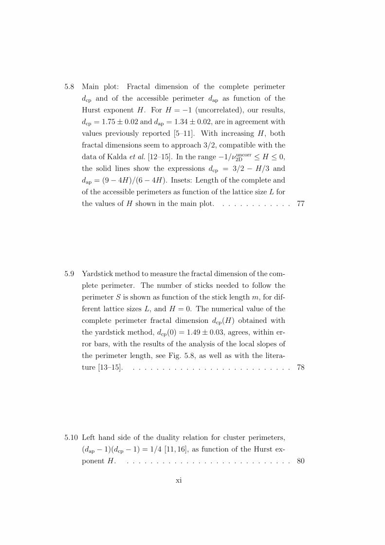
5.8 Main plot: Fractal dimension of the complete perimeter
dcp and of the accessible perimeter dap as function of the
Hurst exponent H. For H = −1 (uncorrelated), our results,
dcp = 1.75± 0.02 and dap = 1.34± 0.02, are in agreement with
values previously reported [5–11]. With increasing H, both
fractal dimensions seem to approach 3/2, compatible with the
data of Kalda et al. [12–15]. In the range −1/νuncorr2D ≤ H ≤ 0,
the solid lines show the expressions dcp = 3/2 − H/3 and
dap = (9− 4H)/(6− 4H). Insets: Length of the complete and
of the accessible perimeters as function of the lattice size L for
the values of H shown in the main plot. . . . . . . . . . . . . 77
5.9 Yardstick method to measure the fractal dimension of the com-
plete perimeter. The number of sticks needed to follow the
perimeter S is shown as function of the stick length m, for dif-
ferent lattice sizes L, and H = 0. The numerical value of the
complete perimeter fractal dimension dcp(H) obtained with
the yardstick method, dcp(0) = 1.49± 0.03, agrees, within er-
ror bars, with the results of the analysis of the local slopes of
the perimeter length, see Fig. 5.8, as well as with the litera-
ture [13–15]. . . . . . . . . . . . . . . . . . . . . . . . . . . . 78
5.10 Left hand side of the duality relation for cluster perimeters,
(dap − 1)(dcp − 1) = 1/4 [11, 16], as function of the Hurst ex-
ponent H. . . . . . . . . . . . . . . . . . . . . . . . . . . . . 80
xi
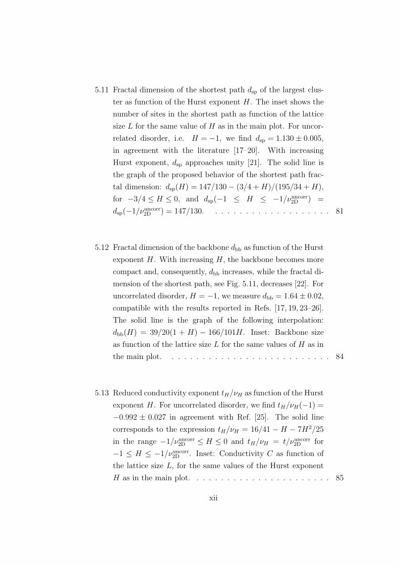
5.11 Fractal dimension of the shortest path dsp of the largest clus-
ter as function of the Hurst exponent H. The inset shows the
number of sites in the shortest path as function of the lattice
size L for the same value of H as in the main plot. For uncor-
related disorder, i.e. H = −1, we find dsp = 1.130± 0.005,
in agreement with the literature [17–20]. With increasing
Hurst exponent, dsp approaches unity [21]. The solid line is
the graph of the proposed behavior of the shortest path frac-
tal dimension: dsp(H) = 147/130− (3/4 +H)/(195/34 +H),
for −3/4 ≤ H ≤ 0, and dsp(−1 ≤ H ≤ −1/νuncorr2D ) =
dsp(−1/νuncorr2D ) = 147/130. . . . . . . . . . . . . . . . . . . . 81
5.12 Fractal dimension of the backbone dbb as function of the Hurst
exponent H. With increasing H, the backbone becomes more
compact and, consequently, dbb increases, while the fractal di-
mension of the shortest path, see Fig. 5.11, decreases [22]. For
uncorrelated disorder, H = −1, we measure dbb = 1.64± 0.02,
compatible with the results reported in Refs. [17, 19, 23–26].
The solid line is the graph of the following interpolation:
dbb(H) = 39/20(1 + H) − 166/101H. Inset: Backbone size
as function of the lattice size L for the same values of H as in
the main plot. . . . . . . . . . . . . . . . . . . . . . . . . . . 84
5.13 Reduced conductivity exponent tH/νH as function of the Hurst
exponent H. For uncorrelated disorder, we find tH/νH(−1) =
−0.992 ± 0.027 in agreement with Ref. [25]. The solid line
corresponds to the expression tH/νH = 16/41 −H − 7H2/25
in the range −1/νuncorr2D ≤ H ≤ 0 and tH/νH = t/νuncorr
2D for
−1 ≤ H ≤ −1/νuncorr2D . Inset: Conductivity C as function of
the lattice size L, for the same values of the Hurst exponent
H as in the main plot. . . . . . . . . . . . . . . . . . . . . . . 85
xii
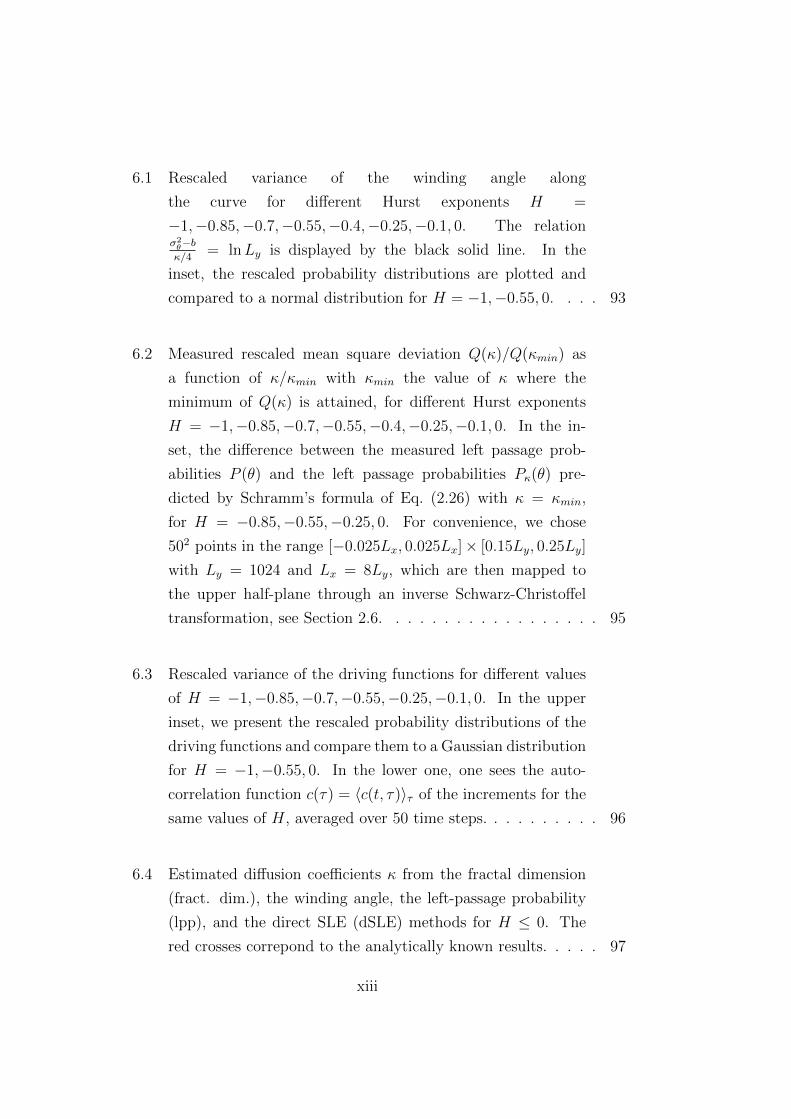
6.1 Rescaled variance of the winding angle along
the curve for different Hurst exponents H =
−1,−0.85,−0.7,−0.55,−0.4,−0.25,−0.1, 0. The relationσ2θ−bκ/4
= lnLy is displayed by the black solid line. In the
inset, the rescaled probability distributions are plotted and
compared to a normal distribution for H = −1,−0.55, 0. . . . 93
6.2 Measured rescaled mean square deviation Q(κ)/Q(κmin) as
a function of κ/κmin with κmin the value of κ where the
minimum of Q(κ) is attained, for different Hurst exponents
H = −1,−0.85,−0.7,−0.55,−0.4,−0.25,−0.1, 0. In the in-
set, the difference between the measured left passage prob-
abilities P (θ) and the left passage probabilities Pκ(θ) pre-
dicted by Schramm’s formula of Eq. (2.26) with κ = κmin,
for H = −0.85,−0.55,−0.25, 0. For convenience, we chose
502 points in the range [−0.025Lx, 0.025Lx]× [0.15Ly, 0.25Ly]
with Ly = 1024 and Lx = 8Ly, which are then mapped to
the upper half-plane through an inverse Schwarz-Christoffel
transformation, see Section 2.6. . . . . . . . . . . . . . . . . . 95
6.3 Rescaled variance of the driving functions for different values
of H = −1,−0.85,−0.7,−0.55,−0.25,−0.1, 0. In the upper
inset, we present the rescaled probability distributions of the
driving functions and compare them to a Gaussian distribution
for H = −1,−0.55, 0. In the lower one, one sees the auto-
correlation function c(τ) = 〈c(t, τ)〉τ of the increments for the
same values of H, averaged over 50 time steps. . . . . . . . . . 96
6.4 Estimated diffusion coefficients κ from the fractal dimension
(fract. dim.), the winding angle, the left-passage probability
(lpp), and the direct SLE (dSLE) methods for H ≤ 0. The
red crosses correpond to the analytically known results. . . . . 97
xiii

6.5 Rescaled variance of the winding angle along the curve for
different Hurst exponents H = 0, 0.1, 0.25, 0.55, 0.7, 0.95. The
relationσ2θ−bκ/4
= lnLy is displayed by the black solid line. In
the inset, the rescaled probability distributions are plotted and
compared to a normal distribution for the same values of H. . 99
6.6 Measured rescaled mean square deviation Q(κ)/Q(κmin) as
a function of κ, with κmin the value of κ where the min-
imum of Q(κ) is attained, for different Hurst exponents
H = 0, 0.1, 0.25, 0.55, 0.7, 0.95. For convenience, we chose 502
points in the range [−0.025Lx, 0.025Lx]×[0.15Ly, 0.25Ly] with
Ly = 1024 and Lx = 8Ly, which are then mapped to the upper
half-plane through an inverse Schwarz-Christoffel transforma-
tion, see Section 2.6. . . . . . . . . . . . . . . . . . . . . . . . 100
6.7 Rescaled variance of the driving functions for different val-
ues of H = 0, 0.1, 0.25, 0.55, 0.7, 0.95. In the upper inset, we
present the rescaled probability distributions of the driving
functions and compare them to a Gaussian distribution for
the same values of H. . . . . . . . . . . . . . . . . . . . . . . . 101
6.8 Estimated diffusion coefficients κ from the fractal dimension
(fract. dim.), the winding angle, the left-passage probability
(lpp), and the direct SLE (dSLE) methods for H ≥ 0. The
red cross correponds to the analytically known result for H = 0.102
6.9 Auto-correlation function c(τ) = 〈c(t, τ)〉τ , averaged over 50
time steps, displayed in log-log scale for values of the Hurst
exponent H = −0.7,−0.55,−0.25, 0, 0.25, 0.55, 0.7. . . . . . . 104
6.10 Rescaled variance 4(σ2θ − b)/κ of the winding angle for the
shortest path in the percolating cluster for values of the Hurst
exponent H = −1,−0.85,−0.7,−0.55,−0.4,−0.25,−0.1, 0.
In the inset, the variance σ2θ is shown. . . . . . . . . . . . . . . 106
6.11 Rescaled variance 4(σ2θ − b)/κ of the winding angle for the
watershed lines in random surfaces of Hurst exponents H =
−1,−0.85,−0.7,−0.55,−0.4,−0.25,−0.1, 0. In the inset, the
variance σ2θ is shown. . . . . . . . . . . . . . . . . . . . . . . . 107
xiv
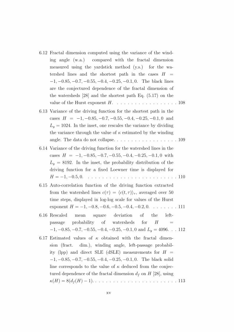
6.12 Fractal dimension computed using the variance of the wind-
ing angle (w.a.) compared with the fractal dimension
measured using the yardstick method (y.s.) for the wa-
tershed lines and the shortest path in the cases H =
−1,−0.85,−0.7,−0.55,−0.4,−0.25,−0.1, 0. The black lines
are the conjectured dependence of the fractal dimension of
the watersheds [28] and the shortest path Eq. (5.17) on the
value of the Hurst exponent H. . . . . . . . . . . . . . . . . . 108
6.13 Variance of the driving function for the shortest path in the
cases H = −1,−0.85,−0.7,−0.55,−0.4,−0.25,−0.1, 0 and
Ly = 1024. In the inset, one rescales the variance by dividing
the variance through the value of κ estimated by the winding
angle. The data do not collapse. . . . . . . . . . . . . . . . . . 109
6.14 Variance of the driving function for the watershed lines in the
cases H = −1,−0.85,−0.7,−0.55,−0.4,−0.25,−0.1, 0 with
Ly = 8192. In the inset, the probability distribution of the
driving function for a fixed Loewner time is displayed for
H = −1,−0.5, 0. . . . . . . . . . . . . . . . . . . . . . . . . . 110
6.15 Auto-correlation function of the driving function extracted
from the watershed lines c(τ) = 〈c(t, τ)〉τ , averaged over 50
time steps, displayed in log-log scale for values of the Hurst
exponent H = −1,−0.8,−0.6,−0.5,−0.4,−0.2, 0. . . . . . . . 111
6.16 Rescaled mean square deviation of the left-
passage probability of watersheds for H =
−1,−0.85,−0.7,−0.55,−0.4,−0.25,−0.1, 0 and Ly = 4096. . . 112
6.17 Estimated values of κ obtained with the fractal dimen-
sion (fract. dim.), winding angle, left-passage probabil-
ity (lpp) and direct SLE (dSLE) measurements for H =
−1,−0.85,−0.7,−0.55,−0.4,−0.25,−0.1, 0. The black solid
line corresponds to the value of κ deduced from the conjec-
tured dependence of the fractal dimension df on H [28], using
κ(H) = 8(df (H)− 1). . . . . . . . . . . . . . . . . . . . . . . . 113
xv

6.18 Estimated diffusion coefficients κ from the fractal dimension
(fract. dim.), the winding angle, the left-passage probability
(lpp), and the direct SLE (dSLE) methods for H ∈ [−1, 1].
The red crosses correpond to the analytically known result for
H = −1, i.e. percolation, and H = 0, i.e. the GFF. We
see that the results are compatible with SLE for H ≤ 0 but
incompatible for H > 0. . . . . . . . . . . . . . . . . . . . . . 116
7.1 Graphene membrane after thermalisation. Inset: The blue
points represent carbon atoms that are above the isoheight
plane. The red line shows the extracted path along the inter-
section between the membrane and the isoheight plane. . . . . 121
7.2 The function H(r), as defined in the main text, computed
for the inner carbon atoms of the graphene membrane. Main
panel: The function H(r) for different system sizes at T = 300
K. Inset: The function H(r) for different temperatures for a
system of 800A× 800A. . . . . . . . . . . . . . . . . . . . . . 124
7.3 Main panel: Fractal dimension of the isoheight contour lines
computed with the yardstick method for a fixed temperature
T = 300 K and different system sizes. We find a universal
fractal dimension of df = 1.28±0.05. Inset: Fractal dimension
df for different temperatures and fixed system size of 800A×800A. The solid line denotes the slope −df = −1.28. . . . . . 125
7.4 Fractal dimension of the area enclosed by the isoheight contour
lines of the spanning clusters, computed with the box counting
method. The number N of boxes used to cover the atoms
belonging to the spanning cluster is displayed as a function
of the lateral size r of the boxes. Main panel: Box counting
method for different system sizes at T = 300 K. Inset: Box
counting method for different temperatures for a system size
of 800A× 800A. . . . . . . . . . . . . . . . . . . . . . . . . . . 126
xvi
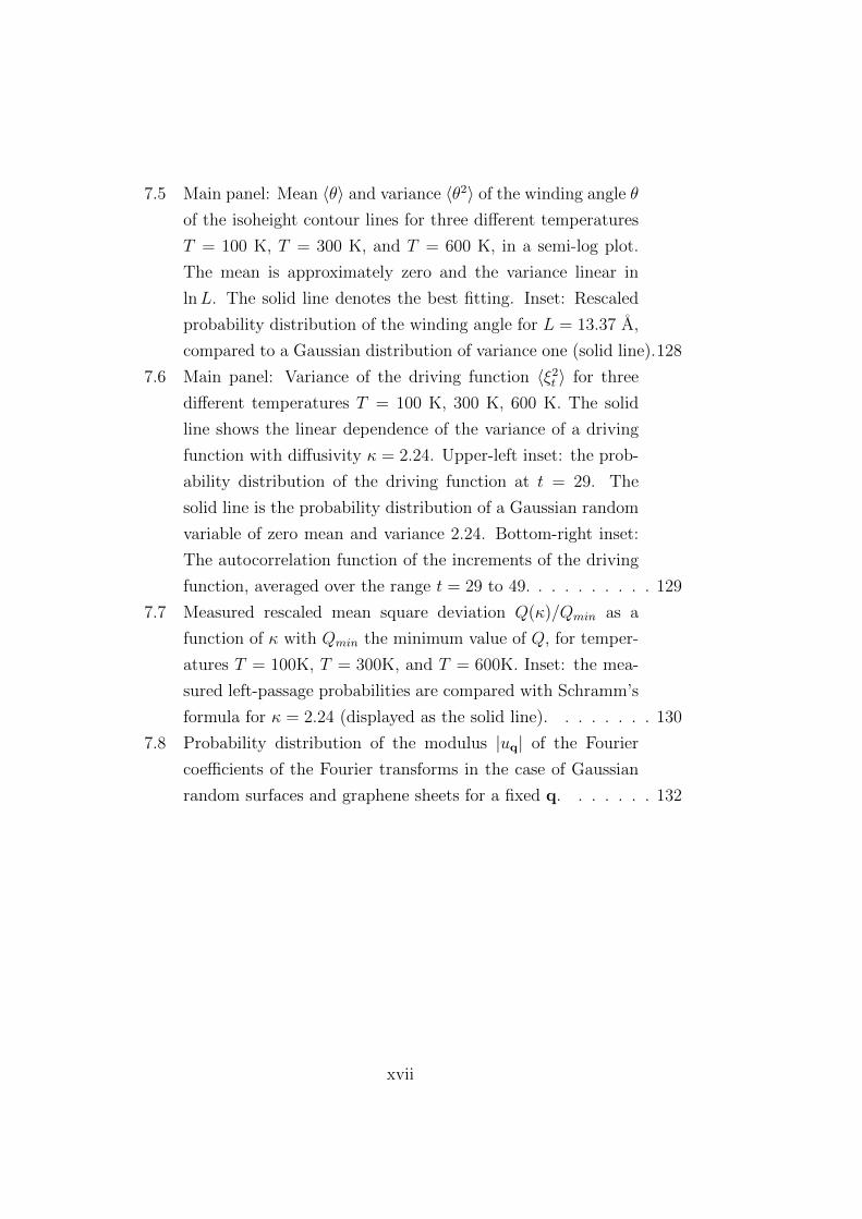
7.5 Main panel: Mean 〈θ〉 and variance 〈θ2〉 of the winding angle θ
of the isoheight contour lines for three different temperatures
T = 100 K, T = 300 K, and T = 600 K, in a semi-log plot.
The mean is approximately zero and the variance linear in
lnL. The solid line denotes the best fitting. Inset: Rescaled
probability distribution of the winding angle for L = 13.37 A,
compared to a Gaussian distribution of variance one (solid line).128
7.6 Main panel: Variance of the driving function 〈ξ2t 〉 for three
different temperatures T = 100 K, 300 K, 600 K. The solid
line shows the linear dependence of the variance of a driving
function with diffusivity κ = 2.24. Upper-left inset: the prob-
ability distribution of the driving function at t = 29. The
solid line is the probability distribution of a Gaussian random
variable of zero mean and variance 2.24. Bottom-right inset:
The autocorrelation function of the increments of the driving
function, averaged over the range t = 29 to 49. . . . . . . . . . 129
7.7 Measured rescaled mean square deviation Q(κ)/Qmin as a
function of κ with Qmin the minimum value of Q, for temper-
atures T = 100K, T = 300K, and T = 600K. Inset: the mea-
sured left-passage probabilities are compared with Schramm’s
formula for κ = 2.24 (displayed as the solid line). . . . . . . . 130
7.8 Probability distribution of the modulus |uq| of the Fourier
coefficients of the Fourier transforms in the case of Gaussian
random surfaces and graphene sheets for a fixed q. . . . . . . 132
xvii

xviii
Zusammenfassung
In statistischer Physik interessiert man sich hauptsachlich dafur, Zufalls-
pfade und deren Prozesse durch ihre kritischen Eigenschaften zu klassi-
fizieren, um Ahnlichkeiten zwischen Prozessen herauszufinden, die bei er-
ster Betrachtung unterschiedliche Eigenschaften zu haben scheinen. In der
vorliegenden Arbeit studieren wir Zufallspfade im Rahmen der Schramm-
Loewner Evolution Theorie (SLE). SLE stellt einen allgemeinen Rahmen dar,
der uber die traditionelle Analyse hinausgeht, die auf kritischen Exponenten
beruht. Die Analyse mithilfe von SLE fuhrt dazu, Pfade durch eine eindimen-
sionale Brownsche Bewegung zu beschreiben. Die Statistiken dieser Pfade
spiegeln sich im Diffusionskoeffizienten der Brownschen Bewegung wieder.
Um die SLE-Eigenschaften der stochastischen Prozesse zu untersuchen, be-
nutzen wir vier verschiedene Tests, um festzustellen, ob die Statistiken der
Zufallspfade mit der SLE- Statistik ubereinstimmen. Wir studieren Zufallsp-
fade, die entweder von Standard-Modellen der statistischen Physik stammen
oder die an stochastische Flachen gekoppelt sind. Eine der wenigen noch
unbeantworteten Fragen zur unkorrelierten Perkolationstheorie ist, welche
fraktale Dimension der kurzeste Pfad hat. Es gab mehrere Versuche, sie
exakt zu berechnen, was zu mehreren Vermutungen gefuhrt hat, die sich
aber alle als unrichtig erwiesen haben. Deswegen sollte man dieses Prob-
lem mit einem neuen Ansatz angehen, wobei die SLE-Theorie ein solcher
Ansatz sein konnte. Wir haben getestet, ob der kurzeste Pfad durch die
SLE-Theorie beschrieben werden kann, und haben numerische Beweise fur
SLE-Statistik gefunden. Dies lasst es als moglich erscheinen, eine analytis-
che Rechnung der fraktalen Dimension des kurzesten Pfades zu entwickeln.
1
Im Gegensatz zur unkorrelierten Perkolationstheorie haben Systeme aus der
Natur weitreichende Korrelationen. Deswegen haben wir uns auch dafur
interessiert, weitreichende korrelierte Systeme zu studieren. Insbesondere
haben wir Systeme analysiert, die an stochastische Flachen gekoppelt sind,
die weitreichende Korrelationen haben, die durch den Hurst-Exponenten H
beschrieben sind. Zuerst haben wir die Eigenschaften der Perkolation auf
solchen Flachen analysiert, darunter die fraktale Dimension des perkolieren-
den Clusters und dessen Grenzpfade. Wir haben auch die geometrischen
Eigenschaften des großten Clusters studiert. Da es mathematisch bewiesen
wurde, dass die Grenzpfade des perkolierenden Clusters fur unkorrelierte
Perkolation der SLE-Theorie folgen, haben wir uns gefragt, ob solch ein Re-
sultat auch fur korrelierte Perkolation gultig ist. Wir haben herausgefunden,
dass die Statistiken des zuganglichen Perimeters fur H ∈ [−1, 0] mit der
SLE-Statistik kompatibel sind, aber nicht fur H ∈ (0, 1], und haben eine
Abhangigkeit zwischen dem Hurst-Exponenten H ≤ 0 der Landschaft und
dem Diffusionskoeffizienten der Brownschen Bewegung aufgezeigt. Dieses
Resultat erweitert zwei analytisch bewiesene Ergebnisse und konnte zu inter-
essanten Entwicklungen im Bereich derjenigen Pfade fuhren, die an Flachen
gekoppelt sind. Dieses Resultat hat jedoch auch Folgen fur Systeme, die man
als stochastische Flachen betrachten kann. Wir haben die SLE-Theorie auf
eine spezifische Flache, und zwar Graphen, angewendet, und haben herausge-
funden, dass die Isolinien auch Statistiken darstellen, die mit SLE kompatibel
sind.
2

Summary
In Statistical Physics, one is usually interested in classifying random curves
and their associated processes according to their critical properties, in order
to draw similarities between processes that seem at first to have different
properties. Here we are interested in the study of random curves in the
framework of Schramm-Loewner Evolution (SLE) theory. SLE provides a
general framework that goes beyond the traditional analysis based on critical
exponents. In fact, it provides a way to describe curves starting from a
generalized one-dimensional Brownian motion, where the statistics of the
curve is encoded in the diffusivity. Here, in order to get insights into the
SLE properties of random processes, we use four different numerical tests to
verify if the statistics of the random paths are compatible with SLE statistics.
In this thesis we study random curves, whether related to standard Statistical
Physics models or coupled to random surfaces.
One of the open question regarding random uncorrelated percolation is the
value of the fractal dimension of the shortest path. There has been many
attempts to compute it exactly, leading to many conjectures that have been
ruled out. Therefore, it seems that a new approach has to be found to
tackle this problem, and the SLE theory might be one. We tested if the
shortest path might be described by SLE, and found numerical evidence for
SLE statistics. This result opens the possibility to develop an analytical
framework to compute the fractal dimension of the shortest path, one of the
last critical exponent in percolation, whose exact value is unknown.
But as in nature, systems exhibit long-range correlations, we went beyond
the framework of usual uncorrelated percolation, and studied long-range cor-
3
related systems associated to random surfaces that display long-range cor-
relations characterized by their Hurst exponent H. First, we studied the
critical properties of percolation associated to these surfaces, studying the
fractal dimension of the percolating cluster and its boundaries, as well as the
geometrical and transport properties of the largest cluster. As the cluster
boundaries of the percolating clusters have been shown analytically to be SLE
for uncorrelated percolation, we wondered if this property applies also for the
boundaries of clusters in correlated percolation. We found that the accessible
perimeter displays statistics compatible with SLE in the range H ∈ [−1, 0],
but not for H > 0, and got a dependance of the diffusion exponent of the
underlying Brownian motion on the value of the Hurst exponent H ≤ 0 of
the surface. This result might lead to interesting developments concerning
the coupling between random surfaces and SLE, as it extends two exactly
known analytical results. But it also has consequences on the properties of
physical systems that can be seen as random surfaces. We applied the SLE
theory to one specific rough surface, suspended graphene sheet, and found
that isoheight lines present statistics compatible with SLE.
4

Resume
En Physique Statistique, on s’attache communement a la classification de
courbes aleatoires et des processus qui leur sont associes en fonction de
leurs proprietes critiques, afin d’etablir des similarites entre des processus
qui semblent a priori tres differents. Dans la presente these, nous nous
interessons a l’etude de courbes aleatoires dans le contexte des evolutions
de Schramm-Loewner (SLE). La theorie SLE constitue un cadre general qui
depasse l’approche traditionnelle basee sur l’etude des exposants critiques.
Elle permet de decrire des courbes aleatoires a partir d’un mouvement brown-
ien unidimensionnel dont le coefficient de diffusivite encode les proprietes
statistiques des courbes aleatoires. Afin d’etudier les proprietes SLE de pro-
cessus stochastiques, nous utilisons quatre tests numeriques differents pour
verifier si les statistiques des courbes aleatoires sont compatibles avec les
statistiques de processus SLE. Dans le present travail, nous etudions des
courbes aleatoires associees soit a des modeles usuels de la Physique Statis-
tique, soit a des surfaces aleatoires.
La valeur de la dimension fractale du chemin le plus court constitue l’une des
dernieres questions ouvertes dans la theorie de la percolation. Il y a eu de
multiples approches pour tenter de la calculer, conduisant a l’etablissement de
nombreuses conjectures qui ont toutes ete ecartees. C’est pourquoi il semble
necessaire de trouver une nouvelle approche pour aborder ce probleme, et
la theorie SLE pourrait en etre une. Nous avons par consequent teste si le
chemin le plus court dans le modele de percolation peut etre decrit par la
theorie SLE. Nous avons trouve un accord numerique avec les predictions
de la theorie SLE. Ce resultat ouvre la possibilite de developper un cadre
5
analytique permettant de calculer la dimension fractale du chemin le plus
court, l’un des derniers exposants critiques de la percolation dont on ignore
encore la valeur exacte.
Mais comme dans la nature les systemes presentent des correlations longue
portee, nous avons depasse le cadre de la percolation non correlee usuelle,
et avons etudie des systemes correles associes a des surfaces presentant des
correlations longue portee caracterisees par leur exposant de Hurst H. Dans
un premier temps nous avons etudie les proprietes critiques du processus
de percolation associe a ces surfaces, en s’attachant plus particulierement
a l’etude des proprietes fractales de l’amas percolant et de ses contours,
mais aussi aux proprietes geometriques et de transport de l’amas le plus
large. Comme il a ete demontre que le contour de l’amas percolant est decrit
par une evolution de Schramm-Loewner dans le cas de la percolation non
correlee, on peut se demander s’il est possible d’etendre cette propriete aux
contours des amas percolant dans un modele de percolation correlee. Nous
avons trouve que le perimetre accessible presente des proprietes statistiques
compatibles avec une evolution de Schramm-Loewner pour des valeurs de
l’exposant de Hurst comprises entre −1 et 0 mais pas pour des valeurs de H
strictement positives. Nous avons trouve que la valeur du coefficient de diffu-
sion du mouvement Brownien de l’evolution de Schramm-Loewner depend de
la valeur de l’exposant de Hurst H ≤ 0 de la surface. Ce resultat peut con-
duire a des developpements interessants dans le domaine des courbes SLE
associees a des surfaces aleatoires. Cependant cette approche a aussi des
consequences sur l’etude des proprietes de certains systemes physiques vus
comme des surfaces aleatoires. Nous avons par exemple applique la theorie
SLE a des courbes extraites d’une surface particuliere, a savoir une feuille de
graphene suspendue, et avons montre que ses lignes de niveau presentent des
statistiques compatibles avec la theorie SLE.
6
Chapter 1
Introduction
Statistical Physics has been very much attached to study the properties of
curves coming from different physical models, in order to determine if they
share similar properties. This has lead to the classification of models, through
their critical exponents, into universality classes. Especially, the study of Sta-
tistical Physics models reveals interesting fractal curves with fractal dimen-
sions that are the same for different models. But can we find more universal
properties about those curves? A new theory has emerged recently, that
allows to describe curves by a more general framework. It has been discov-
ered by Schramm in 1999 [29] and is called Schramm-Loewner, or stochastic
Loewner, Evolution (SLE) theory. Knowing the fractal dimension of a curve
does not give as much information about the system as being SLE. The SLE
theory gives insights into the statistical distribution of the curves, and more-
over it allows to describe curves belonging to different universality classes by
a same process: a one-dimensional Brownian motion. Loop-Erased Random
Walk (see Fig. 1.1), Self-Avoiding Walk, percolation hulls (see Fig. 1.2), hulls
in the Ising model for example belong to different universality classes but can
be described through the same random process, a Brownian motion, in the
framework of SLE. The free parameter in the SLE theory is the diffusion
coefficient of the one-dimensional Brownian motion that controls the statis-
tical properties of the random curves. Therefore the SLE theory reduces the
properties of the curves to a single parameter. It opens new opportunities for
analytical work and numerical simulation methods. Problems resulting from
1
2 CHAPTER 1. INTRODUCTION
some kinds of optimization processes like watersheds [30], or the shortest
path [31], or from solving complex partial differential equations like in tur-
bulence [32–34] are computationally expensive, and by means of SLE theory
one might develop methods to simulate statistically equivalent curves with
less computational time.
SLE is not only usefull to describe hulls or random processes arizing in Sta-
tistical Physics models but can be also found in random surfaces. Curves
like isoheight lines coupled to random surfaces exhibit SLE properties. This
has first been studied in relation to the Gaussian Free Field (GFF), where
isoheight lines have been shown to be SLE [35, 36]. But it has also been
seen experimentaly or numericaly in physical systems like WO3 grown sur-
faces [37], Kardar-Parisi-Zhang surfaces [38], or turbulences seen as random
surfaces [32–34]. Therefore a natural question is whether isoheight lines give
any insight into the statistics of the surface itself. This question has been
tackled in a very specific case by mathematicians: in the case of the GFF.
There one is able to reconstruct the surface from its isoheights. But if it is
possible to characterize the statistics of other surfaces from their isoheight
lines is still an open question. Very recently, the field of fractional Gaus-
sian Fields [39] has been developed and might give some insights into this
problem.
In this thesis we studied both the SLE theory applied to a classical Statistical
Physics problem, the shortest path in percolation, and in relation to random
surfaces through the study of their isoheight lines.
Chapter 2 gives an introduction to the SLE theory. We derive the Loewner
differential equation, and introduce its stochastic version that is used in SLE.
We also detail the implications of SLE and define the numerical methods we
use to test the compatibility of the studied processes to the SLE theory.
In Chapter 3 we apply SLE theory to a classical Statistical Physics problem,
the shortest path in percolation. The fractal dimension of the shortest path
is one of the last critical exponent of random uncorrelated percolation that
is not known exactly. One wonders if one can apply the SLE theory to study
this critical curve, as it would give some insights into the critical exponent
of the shortest path. Therefore we test numerically the compatibility of the
2

3
statistics of the shortest path with SLE.
In Chapter 4 we recall some important characteristics of rough surfaces and
random fields. We also describe the so-called Fourier Filtering Method that is
used to generate random fields, and its connection to correlated percolation.
We also give some insights in its relation to so-called fractional Gaussian
fields.
In Chapter 5 we study extensively the properties of long-range correlated
percolation, and its dependance on the so-called Hurst exponent H control-
ling the strength of the correlations. One sees that the properties of the
system are very much dependant on H, and conjecture the dependancy of
the critical exponents of the system on H.
In Chapter 6 we study isoheight lines in long-range correlated surfaces in re-
lation to SLE properties. Isoheight lines on uncorrelated random landscapes
and on the GFF have been analyticaly proven to be SLE. We investigate if
we can extrapolate these two results by tuning the strenght of the correlation
from the uncorrelated case to the GFF case and further to rough surfaces
with strictly positive Hurst exponent. We do the same study for watersheds
in correlated landscapes and the shortest path in correlated percolation and
compare the results of the SLE analysis that we have done for these three
different kinds of paths.
In Chapter 7 we study the properties of suspended graphene sheets in relation
to conformal invariance and SLE. We apply the SLE theory to the isoheight
lines of graphene sheets to show that they satisfy more than scale invariance,
indeed they are conformally invariant. This might lead to a field theoretical
approach of graphene sheets. We also compare the results we have found
for graphene sheets with the results we obtained for the theoretical rough
surfaces that we studied in the previous chapter and study their differences,
opening up the question of the best characterization of rough surfaces, not
only through their Hurst exponent.
3

4 CHAPTER 1. INTRODUCTION
O
Fig. 1.1: Loop-Erased Random Walk Discreate Loop-Erased Random
Walk in the upper half-plane. It has been generated using the transition
probabilities defined in Ref. [1] for a random walk half-plane excursion. The
discreate upper half-plane is defined as Z+ iZ+ = {j + ik, j ∈ Z, k ∈ Z+}.
4

5
Fig. 1.2: Percolation Percolation interface generated on a triangular lattice
in a rectangle with Dirichlet boundary conditions, i.e. with zero value (red
sites) on half of the border and one (blue sites) on the other half. The
interface, displayed as a black solid line, is defined such that the interface
path starting from the bottom line has always a red site on its left and a blue
site on its right.
5
6 CHAPTER 1. INTRODUCTION
6
Chapter 2
Schramm-Loewner Evolution
theory
In this chapter, we review some aspects of the SLE theory that might be
usefull to understand the methods that we will use later. Some proofs will
be skipped, but we refer the interested reader to the following references
[1, 40–45]. The SLE theory is well suited to study curves growing in two-
dimensional domains and in the following the domains under consideration
will always be two dimensional.
Suppose that we have a random curve γt growing in a given domain D. One is
interested in the statistical properties of this curve. This is usually a difficult
problem. However, the Loewner theory simplifies this problem, by reducing
the dimensionality of the problem. It maps any non-intersecting curve γt to
a real function. The idea of the Loewner theory is to define a one-to-one
mapping between a growing set, the curve, and a time serie. In the case of
the SLE theory, the curves one considers are generated by a random process
and the time serie to which they are mapped is a Brownian motion. The
aim of the SLE theory is to encode the statistical properties of the random
curves into a Brownian motion.
Suppose that we have a growing set Kt in a Domain D such that the domain
D \ Kt is simply connected, see Fig. 2.1. The Riemann mapping theorem
ensures that there exists a conformal transformation gt from D \Kt onto D.
7
8 CHAPTER 2. SCHRAMM-LOEWNER EVOLUTION THEORY
Kt=γ[0,t]
D
(γt)t≥0
D\Kt
Fig. 2.1: A growing curve (γt)t≥0 in the domain D, in this case the upper
half-plane. The hull Kt is here defined as the curve taken till time t, and
D \Kt is the domain D from which one substracts Kt.
The idea is to study the properties of this conformal transformation gt and
to relate it to a real-valued path. In the case of stochastic Loewner Evolu-
tion also called Schramm-Loewner Evolution (SLE), this idea is extended to
random families of curves and their distributions. The aim is to encode the
statistical properties of the random curves into a real valued random process,
that corresponds to a Brownian motion in the case of SLE.
This theory brings new insights in the common classification of Statistical
Physics models in different universality classes and their characterization
through critical exponents. It improves the characterization of the processes
as it gives insights into the distribution of the random curves, but at the
same time reduces the properties of the curves to a single parameter and
opens opportunities for analytical work and numerical simulation methods.
The most common SLE processes are chordal SLE, related to curves joing the
origin to the point at infinity in the upper half-plane, radial SLE, related to
curves joining usually 0 to 1 in the open unit disk U, and dipolar SLE, related
to curves joing the origin to the upper border in a slit. In the following, we will
8

2.1. CONFORMAL TRANSFORMATIONS AND HOLOMORPHICFUNCTIONS 9
focus on chordal SLE in the complex upper half-plane H = {z, Im(z) > 0}.
But by conformal invariance, one can study the curves in any simply con-
nected open domain. Indeed, by the Riemann mapping theorem, any non-
empty open simply connected proper1 subset of C admits a bijective confor-
mal map to the open unit disk U in C, see Fig. 2.2. Therefore, one can study
the properties of SLE in a choosen domain, and by conformal invariance,
the results will hold for any conformally equivalent domain, though formulas
might change.
2.1 Conformal transformations and holomor-
phic functions
A conformal transformation of the plane is defined as a mapping w = f(z)
that preserves local angles, i.e. a transformation such that for any two smooth
curves γ and η intersecting at z0, the angle formed between the curves γ and
η at z0 is equal to the angle formed between the curves f ◦ γ and f ◦ η at
f(z0), where f ◦ γ denotes the image of the curve γ by the map f . The
conformal property might be described in terms of the Jacobian matrix be-
ing everywhere a scalar times a rotation matrix. The link between angle
preserving transformations and holomorphic2 transformations with non van-
ishing derivative is done through the Cauchy-Riemann Equations
∂u
∂x=∂v
∂y,
∂u
∂y= −∂v
∂x.
(2.1)
which translates into the Jacobian matrix of f(x + iy) = u(x, y) + iv(x, y)
being of the form: Jf (z0) =
(a b
−b a
), with a, b ∈ R, which corresponds to
a rotation composed with a scaling.
1A proper subset S ⊂ S′ of S′ is a subset that is stricly included in S′, sometimes
denoted as S S′.2A holomorphic function is a complex-valued function that is complex differentiable in
a neighborhood of every point in its domain of definition.
9
10 CHAPTER 2. SCHRAMM-LOEWNER EVOLUTION THEORY
O
O
f(z)= z-iz+i
Fig. 2.2: Conformal mapping of the upper half planeH = {z ∈ C, Im(z) > 0}into the unit disk {z ∈ C, |z| < 1}, using f(z) = z−i
z+i.
Therefore one uses the following definition of a conformal map. A conformal
map or biholomorphism is a bijective holomorphic function f : U → V with
U, V open sets in C. U and V are said to be conformally equivalent if there
exists such an f . f has the property that f ′(z) 6= 0 for all z ∈ U and the
inverse of f is also holomorphic.
An important property of holomorphic functions is that holomorphic func-
tions are analytical3 functions everywhere in the domain of definition.
2.2 The Riemann mapping theorem and its
consequences
A fundamental result in complex analysis is the Riemann mapping theorem.
Let D be a proper open simply connected domain, i.e. D is included in
C but cannot be the whole complex plane. There exists a conformal map
φ : D → D, where D = {z ∈ C, |z| < 1}. Actually there exists many of these
maps, but one can make them unique through the following argument. Let
w ∈ D. Then there exists a unique conformal map φ : D → D such that
φ(w) = 0 and arg(φ′(w)) = 0, or φ′(w) > 0.
3An analytic function is locally given by a converging power serie. Moreover analytic
functions are infinitely differentiable.
10

2.2. THE RIEMANN MAPPING THEOREM AND ITSCONSEQUENCES 11
A subset K of H is called a hull4 if it is bounded in H (included in a ball of
finite radius), H \K is simply connected and K = K ∩H.
In the following, we will be interested in conformal maps gK : H\K → H. By
the Riemann mapping theorem there exists many of them. The uniqueness of
the conformal map results from the condition that gK looks like the identity
at infinity, i.e. gK(z) ∼ z for |z| → ∞.
If K is a hull, there exists a unique conformal map gK : H \ K → H such
that:
lim|z|→∞
gK(z)− z = 0. (2.2)
This is called the hydrodynamic normalization.
Set D = {z : −z−1 ∈ H \ K}. D ⊆ H is a simply connect domain, and a
neighborhood of 0 in H. Therefore, by the Riemann mapping theorem, there
exists a conformal map φ : D → H which, by Schwarz reflection principle
imposing φ(z) = φ(z), can be extended to the lower half-plane and admits
a Taylor expansion around 0. As by the reflection principle, φ is real on a
neighborhood of 0 on the real line, one has that the coefficients must be real,
and gets that for z → 0
φ(z) = a0 + a1z + a2z2 + a3z
3 +O(|z|4), (2.3)
with a0, a1, a2, a3 ∈ R. By fixing φ(0) = 0 and φ′(0) > 0, one gets that
a0 = 0 and a1 > 0. We define gK by gK(z) = −a1φ(−z−1)−1 − a2/a1, which
is a conformal map from H \ K onto H. To prove the uniqueness, set g, h
two conformal maps satisfying the hydrodynamic normalization. Therefore
f = g ◦ h−1 is a conformal automorphism of H such that f(z)− z → 0 when
|z| → ∞, and f(∞) =∞. But the conformal automorphisms of H are of the
form
f(z) =az + b
cz + d, (2.4)
with a, b, c, d ∈ R and ad − bc = 1. In order to have f(∞) = ∞, one needs
to have c = 0 and d 6= 0. In order to have that f(z)− z = 0 when |z| → ∞,
4It is sometimes called a compact H-hull.
11

12 CHAPTER 2. SCHRAMM-LOEWNER EVOLUTION THEORY
Kt
O
gt:ℍ \ Kt →ℍ
ℍ
gt(Kt)
O Ut=gt(γ(t))
ℍ
Fig. 2.3: Mapping gt : H \Kt → H. The hull is shown in blue and is mapped
to the real line by gt.
one needs to have that a/d = 1 and b/d = 0. Therefore f is the identity and
g = h, proving the uniqueness.
Actually we have shown that for |z| → ∞,
gK(z) = z +aKz
+O(|z|−2), (2.5)
with aK ∈ R, called the half-plane capacity.
2.3 Half-plane capacity parametrization
For the following, we will prove that the half-plane capacity aK is positive
and increasing in the sense that aK ≥ 0, aK > 0 if K 6= ∅, and aK ≤ aK′ if
K ⊂ K ′. This will allow us to make a reparametrization of the curve.
Let K be a hull, Bt a complex Brownian motion starting at z ∈ H \K, τ be
the hitting time of Bt for R ∪K, and gK be the conformal map from H \Konto H as defined before. Then for z = iy ∈ H\K, with y > 0, the half-plane
capacity aK is given by
aK = hcap(K) = limy→∞
yEiy(Im(Bτ )). (2.6)
Let us consider z 7→ gK(z)−z. It is a bounded analytic function ofH\K = H,
because it is bounded at ∞ and continuous. Therefore5 z 7→ Im(gK(z)− z)
5The real and imaginary parts of holomorphic functions are harmonic, see Eq. (2.1).
12

2.4. THE LOEWNER DIFFERENTIAL EQUATION AND THEDRIVING FUNCTION 13
is a bounded harmonic function. Let us consider a Brownian motion started
at z ∈ H and τ = inf{t > 0 : Bt /∈ H}. By the optional stopping theorem
Im(gK(z)− z) = Ez (Im(gK(Bτ )−Bτ )) . (2.7)
But by definition of gK , Im(gK(Bτ )) = 0. If one sets z = iy, one gets
Im(gK(iy)− iy) = −Eiy(Im(Bτ )). (2.8)
As y → ∞, gK(iy) = iy + aKiy
+ O(1/y2). Therefore yEiy(Im(Bτ )) = aK +
O(1/y) and one recovers Eq. (2.6). We have that aK ≥ 0 and aK > 0 if
K 6= ∅.Now, let us suppose that K ⊂ K ′ and denote K = K ′ \ K. One considers
the conformal maps defined as before gK : H \K → H and gK : H \ K → Hwith K = gK(K), see Fig. 2.4. One has gK(z) = z + aK
z+ o(1
z) and gK(z) =
z+aKz
+o(1z) for |z| → ∞. Now, one considers f = gK◦gK : H\K ′ → H. It has
the following limited development for |z| → ∞: f(z) = z+aK+aK
z+ o(1
z), i.e.
f satisfies the hydrodynamic normalization. One can also directly consider
gK′ : H\K ′ → H which is the unique conformal map from H\K ′ onto H with
the hydrodynamic normalization. Therefore, by uniqueness: aK′ = aK + aK ,
and aK′ > aK for K ⊂ K ′ and K 6= K ′.
This result is very usefull if one considers a family of increasing hulls (Kt)t≥0
such that Ks is strictly contained into Kt for s < t. Let us consider a simple
curve γ[0, t] growing in the upper half-plane. One defines gt : H \ γ[0, t]→ Hand for |z| → ∞, gt(z) = z +
aγ[0,t]z
+ o(1/z). Indeed it can be shown that
t 7→ aγ[0,t] is increasing in time and continuous. One reparameterize the curve
such that aγ[0,t] = 2t.
2.4 The Loewner differential Equation and
the driving function
The idea behind the Loewner differential Equation is to have a one-to-one
correspondence between a continuous real valued path Wt = gt(γt), where
13
14 CHAPTER 2. SCHRAMM-LOEWNER EVOLUTION THEORY
ℍ
K K'\KK'
ℍ ℍ
K^
gKg
gK
gK^gKg
gK'
Fig. 2.4: Mapping of the compact H-hull K ′ = K ∪ (K ′ \K) using gK′ or the
composition of gK with gK , f = gK ◦ gK .
γt is the tip of the curve grown till time t, and increasing families of hulls
having a certain local growth property, the hulls Kt of the growing curve γt.
Here we show how a random curve satisfying some given conditions that we
will explain later can be mapped onto a time serie (Wt)t≥0. Also the time
serie (Wt)t≥0 characterizes the curve uniquely, i.e. one can go back from Wt
to the curve.
Let us consider a familiy of hulls (Kt)t≥0, increasing in time, i.e. Ks ( Kt
for s < t. Set Ks,t = gKs(Kt \ Ks). We say that (Kt)t≥0 has the local
growth property if diam(Kt,t+ε)→ 0 when ε→ 0+, where diam(Kt,t+ε) is the
diameter of the smallest disk encompassing the compact set Kt,t+ε.
Then one can show that there exists a unique Wt ∈ R such that:
Wt = gt(γt) :=⋂s>0
gt(γ(t, t+ s]). (2.9)
This defines a mapping between the curve and a real-valued path (Wt)t≥0
called the driving function of the curve.
Actually gt satisfies the Loewner differential Equation with the identity map
14

2.4. THE LOEWNER DIFFERENTIAL EQUATION AND THEDRIVING FUNCTION 15
as initial value. For a fixed z ∈ H,
∂tgt(z) =2
gt(z)−Wt
, with g0(z) = z. (2.10)
The function gt(z) is defined till time T (z) =: inf{t ≥ 0 : z ∈ Kt}.One can show that, see for example Prop. 3.46 in [1], there exists C ∈ Rsuch that for all r ∈ R+ and all ξ ∈ R, and for any hull K ⊂ D(ξ, r) and
z /∈ D(ξ, 2r),
|gK(z)− z − aKz − ξ
| ≤ CraK|z − ξ|2
. (2.11)
We consider the curve being parametrized with half-plane capacity, i.e. aKt =
2t, and applies Eq. (2.11) to gKt,t+ε(zt) = zt+ε = gt+ε(z) and zt = gt(z). One
has that Kt,t+ε ⊂ D(Wt, 2diam(Kt,t+ε)), and aKt,t+ε = 2ε. As z ∈ H \Kt, zt
is in H and for small enough ε, zt /∈ D(Wt, 4diam(Kt,t+ε)). Therefore one can
apply Eq. (2.11) to obtain:
|gt+ε(z)− gt(z)− 2ε
gt(z)−Wt
| ≤ 4Cdiam(Kt,t+ε)ε
|gt(z)−Wt|2. (2.12)
By the local growth property, one has that gt+ε(z)−gt(z)ε
= 2gt(z)−Wt
+ o(1),
and one finds the differential Eq. (2.10) satisfied by gt(z) by letting ε going
to zero. This actually only shows that the right side derivative satisfies
Loewner’s differential equation. For a full proof, see Ref. [1].
Eq. (2.10) is very usefull as if one starts from Wt one can solve the Loewner
differential equation and compute gt from which one deduces the curve. But
also, starting from the curve, one has gt and one can compute Wt = gt(γ(t)).
This leads to the one-to-one relation between the growing curve (γt)t≥0 and
a real valued path (Wt)t≥0.
In the cases we will study, simple or self-touching curves, the local growth
property will be fulfilled. In the case of a continuous simple path, Kt =
γ[0, t] ∈ H. But if one starts from the real-valued path (Wt)t≥0, it has to be
smooth enough in order to generate a simple curve γ(t) = g−1t (Wt) [46].
From (Wt)t≥0, one can deduce gt and from g−1t : H → H \ Kt construct
back Kt, i.e. γ(t) in the case of a simple curve. For all y ∈ H and t ≥ 0,
15

16 CHAPTER 2. SCHRAMM-LOEWNER EVOLUTION THEORY
one constructs g−1t (H) =
⋃y∈H{g
−1t (y)}. Then reconstructs the curve as
γ(0, t] = H \ g−1t (H).
Eq. (2.11) has implications for numerical methods used to solve the Loewner
differential equation Eq. (2.10). From Eq. (2.11) one deduces that the solu-
tion of the Loewner differential equation has the following property:
gt(z) = z +2t
z+ o(t) (2.13)
for t small. But if one considers the following vertical slit
γ(0, t] = 2i√t for t > 0,
then gt : H\γ(0, t]→ H satisfying the Loewner differential Equation is given
by:
gt(z) =√z2 + 4t
as it has the following limited development gt(z) = z + 2t/z + O(1/|z|2) for
|z| → ∞. But it also has the same limited development gt(z) = z+2t/z+o(t)
as t → 0. Therefore Eq. (2.13) shows that as a first order approximation,
one can approximate the solution of the Loewner differential Equation by
a vertical slit map for short times, and that the error is of the order of
o(t). This gives an indication on the error of the vertical slit map method
described later. Let us suppose we are given the time serie (Wnδt)n≥0. Then
gnδt = gδt ◦ . . .◦gδt and at each time step if one approximates gδt by a vertical
slit one makes an error of the order of o(δt).
2.5 Schramm-Loewner Evolution theory
In 1999 Schramm considered a stochastic version of Eq. (2.10) and conjec-
tured that is was describing the scaling limit of the Loop-Erased Random
Walk and the Uniform Spanning Tree [29].
If we choose Wt =√κBt, with κ ≥ 0 and (Bt)t≥0 a one-dimensional standard
Brownian motion, then by Eq. (2.10) one constructs a random family of hulls
16

2.5. SCHRAMM-LOEWNER EVOLUTION THEORY 17
0<κ≤4 4<κ<8 8≤κ
Fig. 2.5: For 0 ≤ κ ≤ 4, the curves are simple. For 4 < κ < 8 they are self
touching and for κ ≥ 8 they are space filling
(Kt)t≥0 called SLEκ. Rohde and Schramm [47], and Lawler et al. [48] in the
case κ = 8, showed that SLEκ generates continuous curves.
Let κ ≥ 0 and gt : Ht → H be the solution of the stochastic Loewner
differential equation
∂tgt(z) =2
gt(z)−Wt
,
g0(z) = z.
(2.14)
defined for z ∈ Ht and up to time T (z) := sup{t > 0 : inf [0,t]|Wt−gt(z)| > 0}.There exists almost surely (a.s.) a continuous curve (γt)t≥0 in H such that for
all t ≥ 0, Ht is the unbounded connected component of H\γ[0, t]. Kt = H\Ht
is called the hull of the curve. In case the curve (γt)t≥0 is simple, Kt is the
curve itself. Indeed the curve (γt)t≥0 is defined as
γt = g−1t (Wt). (2.15)
Actually, in the following, SLEκ will refer whether to the increasing family
(Kt)t≥0, or to the conformal maps (gt)t≥0 or to the curve (γt)t≥0 depending
on the context.
Depending on the value of κ, the curve (γt)t≥0 exhibits different properties.
For κ ∈ [0, 4], the curve γ is a.s. simple. For κ ∈ (4, 8) the curve is a.s.
self-touching, whereas for κ ≥ 8 the curve is a.s. spacefilling, see Fig. 2.5.
Suppose the curve γ has a double point, such that γ(t1) = γ(t2) with t1 < t2.
Then if one maps γ(0, t1] to the real axis by gt1 , the curve defined by γt1(s),
17
18 CHAPTER 2. SCHRAMM-LOEWNER EVOLUTION THEORY
with γt1(s) = gt1(γ(t1, s+t1]) touches the real axis at s = t2−t1. By conformal
invariance and domain Markov property (see below) γt1 and γ have the same
law. Therefore, in order to study the probability of γ having double points,
one studies the probability of γ to go back to the real line. Let x be on the
real line. If x is swallowed by Kt at a given time t, then gt(x) = Wt, and the
random process Xt = gt(x)−Wt√κ
hits 0. But dXt = 2κXt− dBt, by symmetry of
Bt and −Bt, and corresponds to a Bessel process of dimension n = 1 + 4κ. It
hits 0 an infinite number of times with probability 1 for n < 2, and does not
hit 0 with probability 1 for n ≥ 2. Therefore the curve γ is simple for κ ≤ 4
and has an infinite number of double points for κ > 4. Actually, for κ > 4
one can show that the hull Kt of the path grows towards H.
We have seen that SLEκ for κ ≤ 4 and κ > 4 exhibits different properties.
However there exists a duality relation between the outer boundary of SLEκ
and SLE16/κ for κ > 4. The outer boundary of SLEκ curves for κ > 4 looks
like SLE16/κ curves.
There is another characterization of SLEκ curves. If a family of random
curves is SLEκ, then it is conformally invariant and satisfies the Domain
Markov Property. And reciprocally, if a family of stochastic curves satisfies
conformal invariance and the Domain Markov property, then there exists a
κ ∈ R+ such that these curves are SLEκ.
Conformal invariance Given two domains D and D′ that are conformally
equivalent, one can transfer the probability from one domain to the other
one by simply mapping the curves into the new domain. Let us consider a
conformal map Φ from the domain D onto the domain D′, Φ : D → D′,
and two points on the boundary of D, a, b ∈ ∂D, which are mapped by Φ to
a′, b′ ∈ ∂D′. The probability measure PD,a,b on the curves γ in D from a to
b induces under Φ a probability measure Φ ∗ PD,a,b on curves in D′ = Φ(D)
from a′ = Φ(a) to b′ = Φ(b):
∀U ⊂ D, Φ ∗ PD,a,b (Φ(γ) ⊂ Φ(U)) := PΦ(D),Φ(a),Φ(b) (Φ(γ) ⊂ Φ(U))
= PD,a,b (γ ⊂ U) .(2.16)
18

2.5. SCHRAMM-LOEWNER EVOLUTION THEORY 19
In this equation, we just transfered the probability measure P between two
conformaly equivalent domains. The conformal invariance is taken in the
scaling limit.
The process is conformally invariant if, in the continuum limit, the mapped
probability measure Φ∗PD,a,b is the same as the probability measure PD′,a′,b′on the continuum limit of lattice curves generated in D′ going from a′ to b′:
∀U ⊂ D, Φ ∗ PD,a,b (γ ⊂ U) = PD′,a′,b′ (Φ(γ) ⊂ Φ(U)) . (2.17)
Domain Markov Property Consider a curve γ in D starting in a and
ending in b. Take a point c belonging to the curve, and consider the two
propability measures, see Fig. 2.6:
1. PD,a,b(·|γ[a,c]
)the probability measure in (D, a, b) on the curves starting
in a and ending in b in the domain D conditionned to start with γ[a,c],
2. and PD\γ[a,c],c,b (·) the probability measure in(D \ γ[a,c], c, b
)on the
curves γ[c,b] starting in c and ending in b in the domain D \ γ[a,c].
The Domain Markov Property (DMP) states that the two probability mea-
sures are equal:
PD,a,b(·|γ[a,c]
)= PD\γ[a,c],c,b (·) . (2.18)
The DMP combined to the conformal invariance property expressed in
Eq. (2.17) becomes,
PD,a,b(·|γ[a,c]
)= Φ ∗ PD,a,b (·) , (2.19)
where Φ : D \ γ[a, c] → D is a conformal map such that Φ(c) = a and
Φ(b) = b. It means that Φ(γ[c,b]) is independant of γ[a,c] and has the same
distribution as the original one for curves from a to b in D [42].
Let us consider a random curve γ, growing in the upper half-plane starting
at the origin and growing towards infinity. We define ft(z) = gt(z) −Wt =
z −Wt + 2tz
+ O(
1|z|2
), which is a conformal map that maps the tip of the
curve γ(t) back to the origin and infinity to infinity. Let t, s > 0. Then, by
19

20 CHAPTER 2. SCHRAMM-LOEWNER EVOLUTION THEORY
b
a
c
PD,a,b(γ[ab]| γ[ac])
γ[ac]
γ[ab]
D b
a
c
γ[cb]
D\γ[ac]
PD\γ[ac],c,b(γ[cb])
Fig. 2.6: The two probability measures in the domains D and D \ γ[a,c]. If
the Domain Markov Property is satisfied, these two probabilities are equal.
the Domain Markov Property and the conformal invariance of SLEκ, one has
that γ[0, s] = ft(γ[t, t + s]) is equal in law to γ[t, t + s] and independant on
γ[0, t′] with t′ ≤ t, see Fig. 2.7. From this one deduces that fs is distributed
like ft+s ◦ f−1t , i.e. ft+s = fs ◦ ft in law. For all fixed t and s > 0, one has:
fs ◦ ft(z) = z − (Wt +Ws) +2(t+ s)
z+O
(1
|z|2
)and ft+s(z) = z −Wt+s +
2(t+ s)
z+O
(1
|z|2
),
(2.20)
and therefore for any fixed t ≥ 0, (Wt+s − Wt)s≥0 has the same law as
(Ws)s≥0, and independant of the past values of (Wt′)t′≤t. We conclude that
(Wt)t≥0 is a random process with independant and stationary increments.
Moreover it is continuous (not proven here, see [1] for a proof), and therefore
there exists κ ∈ R+ and α ∈ R such that Wt =√κBt + αt with (Bt)t≥0 a
standard one-dimensional Brownian motion6. By reflection symmetry around
the imaginary axis, α = 0.
6This comes from the theorem stating that a one dimensional Markov process with
continuous trajectory and stationary increments is a Brownian motion with a prossible
drift term.
20
2.5. SCHRAMM-LOEWNER EVOLUTION THEORY 21
ℍ
O
γ(s)~
ft
ℍγ(t+s)
γ(t)
O
γ[0,t]
γ[t,t+s]
ℍ\γ[0,t]γ(t+s)
γ(t)
O
γℍ\γ[0,t][t,t+s]
Domain Markovproperty
Conformal invariance
Fig. 2.7: Under the assumptions of conformal invariance and Domain Markov
Property, the curves γ(t, t + s] knowing γ[0, t] and γ(0, s] are equal in law.
From this one deduces that the driving function has stationary independant
identically distributed increments, i.e. (Wt+s −Wt)s≥0 has the same law as
(Ws)s≥0. 21
22 CHAPTER 2. SCHRAMM-LOEWNER EVOLUTION THEORY
2.6 Mapping of curves generated in a rectan-
gle into the upper-half plane
In numerical simulations, curves are generated in a bounded domain. Thus,
to employ the chordal SLE formalism one needs to use a conformal map to
map it into the upper half-plane. In the context of this thesis, the curves
we generate numerically, are defined in a lattice enclosed in a rectangle of
size Lx×Ly, starting at the bottom boundary and ending at the upper one.
However, we will use results that are valid for chordal curves, like the left-
passage probability formula computed by Schramm [49], see Section 2.7.3
below, or the chordal Loewner Equation Eq. (2.18). Therefore we have to
map conformally the original curves into the upper half-plane using an inverse
Schwarz-Christoffel transformation [50], mapping one point of the boundary
to the origin and an other point of the boundary to infinity. One usually
supposes that the curve starts at the middle point of the bottom edge and
end at the middle point of the top edge. Then, by mapping the first point to
the origin and the second to infinity, the curves generated in the rectangle are
mapped conformally to chordal curves. But if the curves are generated with
“free” boundary conditions, i.e. without any constraints on the boundaries,
such that the paths have no fixed starting and ending points, we relocate
them, in order for them to start at the origin; the curves are now defined in
the rectangle [−Lx, Lx]× [0, Ly] in lattice units. We then make the approxi-
mation, that the curves are defined in the rectangle [−Lx, Lx]× [0, 2Ly], and
that the generated curve is part of a curve starting at the origin and ending
at the point (0, 2Ly). We then use an inverse Schwarz-Christoffel transfor-
mation that maps the rectangle [−Lx, Lx]× [0, 2Ly] onto the upper half plane
with the point (0, 2Ly) being mapped to infinity.
Applying the Schwarz-Christoffel formula for a half-plane to the rectangle
defined in the complex plane as R = (−K,K,K + iK ′,−K + iK ′), one
22
2.7. NUMERICAL TESTS OF SCHRAMM-LOEWNER EVOLUTION 23
obtains the conformal map f : z ∈ H→ w ∈ R [50, 51]:
w = f(z, k)
w =
∫ z
0
dζ√(1− ζ2) (1− k2ζ2)
w =
∫ sin−1 z
0
dθ√1− k2 sin2 θ
w = F(sin−1 z, k
),
(2.21)
with F (φ, k) the elliptic integral of the first kind, and k the elliptic modulus7.
Therefore, from the inversion of the elliptic integral, one gets that
z = f−1(w, k) = sn(w, k), (2.22)
where sn(·, k) is the sine Jacobi elliptic function of modulus k8. The obtained
mapping maps the points w1 = −K, w2 = K, w3 = K + iK ′ and w4 =
−K + iK ′ to the point z1 = −1, z2 = 1 and z3 = k−1 and z4 = −k−1,
with K = K(k) and K ′ = K(√
1− k2), where K(k) =∫ π/2
0dθ√
1−k2 sin2 θis the
complete elliptic integral of the first kind. One needs to adapt the parameter
k to the geometry of the rectangle, i.e. find k such that
K ′(k)
2K(k)=LyLx. (2.23)
Therefore, by solving Eq. (2.23) and applying the inverse Schwarz-Christoffel
transformation sn(·, k) from the rectangle to the upper half-plane, one maps
the generated curves into chordal ones. In the following we will work with
chordal curves.
2.7 Numerical tests of Schramm-Loewner
Evolution
In order to test numerically the agreement of the statistics of the random
curves obtained from physical models with the SLE theory, one uses some
7with 0 < k < 1.8Sometimes the elliptic integrals and Jacobi elliptic functions are denoted with the
parameter m = k2.
23
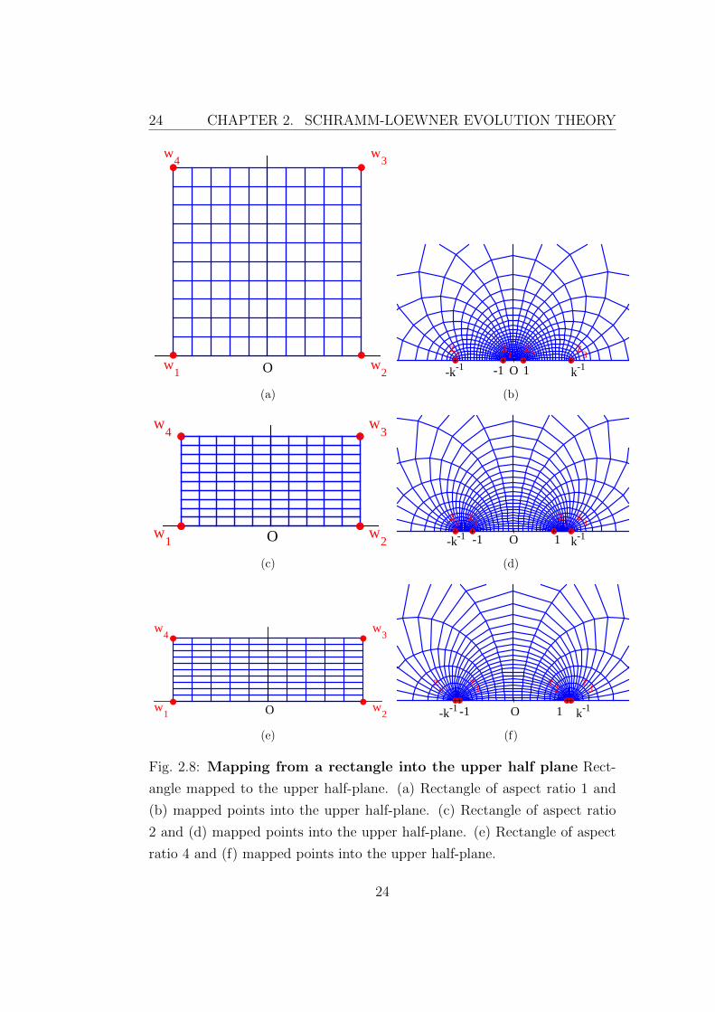
24 CHAPTER 2. SCHRAMM-LOEWNER EVOLUTION THEORY
Ow1
w2
w3
w4
(a)
O-1 1-k-1 k-1
z1
z2
z3
z4
(b)
Ow1
w2
w3
w4
(c)
O-1 1-k-1 k-1
z1
z2
z3
z4
(d)
Ow1
w2
w3
w4
(e)
O-1 1-k-1 k-1
z1
z2
z3
z4
(f)
Fig. 2.8: Mapping from a rectangle into the upper half plane Rect-
angle mapped to the upper half-plane. (a) Rectangle of aspect ratio 1 and
(b) mapped points into the upper half-plane. (c) Rectangle of aspect ratio
2 and (d) mapped points into the upper half-plane. (e) Rectangle of aspect
ratio 4 and (f) mapped points into the upper half-plane.
24
2.7. NUMERICAL TESTS OF SCHRAMM-LOEWNER EVOLUTION 25
properties of SLE curves to test the compatibility of the statistics of the
random curves with the predictions made by the SLE theory. We use in par-
ticular four tests: the fractal dimension, the winding angle, the left-passage
probability and the diffusion of the driving function.
2.7.1 The fractal dimension
The fractal dimension of a curve is defined as follows. If N(r) is the number
of balls of radius r needed to recover a fractal curve, then it scales as N(r) ∼r−df , where df is the fractal dimension of the curve. As has been proven by
Beffara [52], SLEκ curves are fractal with a fractal dimension df depending
on the value of the diffusion coefficient κ as:
df = min(
2, 1 +κ
8
). (2.24)
This constitutes the first way to relate SLE theory to universality classes
characterized through their fractal dimensions. If one wants to show the
SLE behavior of some curves, one uses this relation (2.24) to estimate the
value of κ.
There are several methods to compute the fractal dimension of a curve. We
used the yardstick method, where one approximates the curve by sticks of
different lengths r.
2.7.2 The winding angle
In SLEκ theory, the statistics of the winding of the curve is related to the
value of κ. This result is a consequence of the conformal invariance of the
SLEκ curves.
The winding angle θ between two points X and Y of a curve is defined as
the continuous angle along the curve. Duplantier and Saleur in Ref. [53]
computed the probability distribution of the winding angle of random curves
using conformal invariance and Coulomb gas techniques. As the Coulomb
gas constant is related to κ, one deduces the probability distribution of SLEκ
curves.
25
26 CHAPTER 2. SCHRAMM-LOEWNER EVOLUTION THEORY
In the case of SLE, Schramm [29] proved the convergence of the winding angle
distribution of SLEκ to a Gaussian of variance κ ln(L). Using the relation
κ = 4g, the result obtained through non rigourous Coulomb gas arguments
in [53] is in agreement with the one obtained by Schramm.
In our numerical tests, we compute the variance of the winding angle along all
the points of the curve, instead of the endpoints only, following the relation
obtained by Wieland and Wilson in [54].
For each path, we have a discrete set of points zi on the lattice. We compute
the winding angle θi at each edge zi of the curve iteratively: θi+1 = θi + αi,
where αi is the turning angle between the two consecutive points zi and zi+1,
see Fig. 2.9. Then for SLEκ, the winding angle along all the edges of the
curve exhibits a Gaussian distribution of variance
〈θ2〉 − 〈θ〉2 = b+κ
4ln(Ly), (2.25)
where b is a constant and Ly is the vertical lattice size [54]. The mean value
of the winding angle 〈θ〉 is expected to be zero. Therefore κ is given by the
slope of the graph 〈θ2〉 vs ln(Ly) up to a factor 4.
This test is actually not rigorously a SLE test, as it is considered as a
conformal invariance test. It has for example been used to show the conformal
invariance of rocky shorelines [55]. Therefore, the winding angle test gives
an indication on conformal invariance of the problem, a necessary condition
for SLE. Given the simplicity of this test, we always start with it.
2.7.3 The left-passage probability
A chordal curve, starting at the origin and growing towards infinity, splits
the space into two parts: the points that are at the left of the curve and the
ones that are at the right. The curve is said to pass at the left of a given point
if this point belongs to the right side of the curve, see Fig. 2.10. For chordal
SLEκ curves, Schramm has computed the probability of a curve to go to the
left of a given point z = Reiφ, where R and φ are the polar coordinates of
z [49]. For a chordal SLEκ curve in H, the probability Pκ(φ) that it passes
26
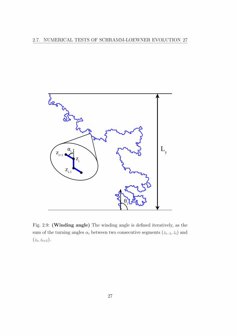
2.7. NUMERICAL TESTS OF SCHRAMM-LOEWNER EVOLUTION 27
θ1
αi
zi
zi+1
zi-1
Ly
Fig. 2.9: (Winding angle) The winding angle is defined iteratively, as the
sum of the turning angles αi between two consecutive segments (zi−1, zi) and
(zi, zi+1).
27
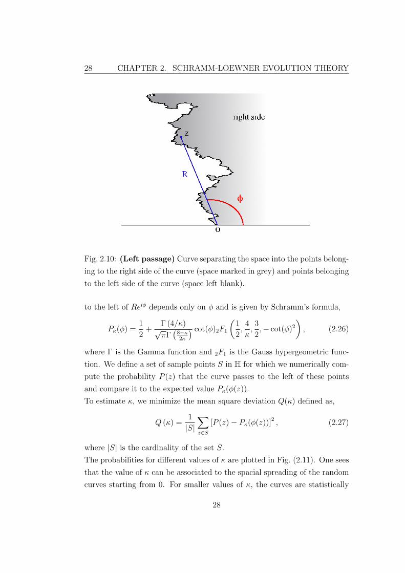
28 CHAPTER 2. SCHRAMM-LOEWNER EVOLUTION THEORY
Fig. 2.10: (Left passage) Curve separating the space into the points belong-
ing to the right side of the curve (space marked in grey) and points belonging
to the left side of the curve (space left blank).
to the left of Reiφ depends only on φ and is given by Schramm’s formula,
Pκ(φ) =1
2+
Γ (4/κ)√πΓ(
8−κ2κ
) cot(φ)2F1
(1
2,
4
κ,3
2,− cot(φ)2
), (2.26)
where Γ is the Gamma function and 2F1 is the Gauss hypergeometric func-
tion. We define a set of sample points S in H for which we numerically com-
pute the probability P (z) that the curve passes to the left of these points
and compare it to the expected value Pκ(φ(z)).
To estimate κ, we minimize the mean square deviation Q(κ) defined as,
Q (κ) =1
|S|∑z∈S
[P (z)− Pκ(φ(z))]2 , (2.27)
where |S| is the cardinality of the set S.
The probabilities for different values of κ are plotted in Fig. (2.11). One sees
that the value of κ can be associated to the spacial spreading of the random
curves starting from 0. For smaller values of κ, the curves are statistically
28
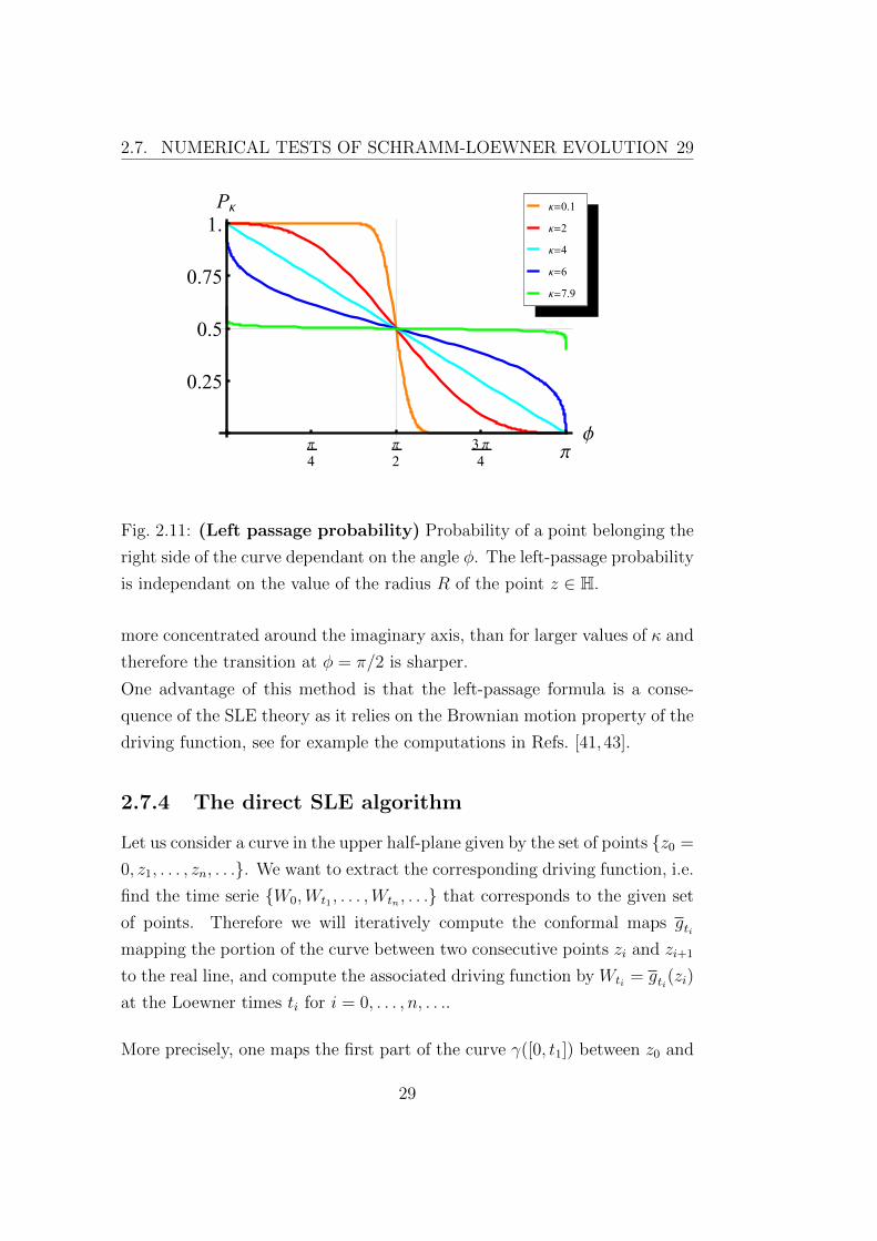
2.7. NUMERICAL TESTS OF SCHRAMM-LOEWNER EVOLUTION 29
Π
4
Π
2
3 Π
4Π
Φ
0.25
0.5
0.75
1.
PΚ
Κ=7.9
Κ=6
Κ=4
Κ=2
Κ=0.1
Fig. 2.11: (Left passage probability) Probability of a point belonging the
right side of the curve dependant on the angle φ. The left-passage probability
is independant on the value of the radius R of the point z ∈ H.
more concentrated around the imaginary axis, than for larger values of κ and
therefore the transition at φ = π/2 is sharper.
One advantage of this method is that the left-passage formula is a conse-
quence of the SLE theory as it relies on the Brownian motion property of the
driving function, see for example the computations in Refs. [41, 43].
2.7.4 The direct SLE algorithm
Let us consider a curve in the upper half-plane given by the set of points {z0 =
0, z1, . . . , zn, . . .}. We want to extract the corresponding driving function, i.e.
find the time serie {W0,Wt1 , . . . ,Wtn , . . .} that corresponds to the given set
of points. Therefore we will iteratively compute the conformal maps gtimapping the portion of the curve between two consecutive points zi and zi+1
to the real line, and compute the associated driving function by Wti = gti(zi)
at the Loewner times ti for i = 0, . . . , n, . . ..
More precisely, one maps the first part of the curve γ([0, t1]) between z0 and
29

30 CHAPTER 2. SCHRAMM-LOEWNER EVOLUTION THEORY
z0=O
z1
z2
z3
ℍ
W0
ℍ
W1
gt1(z2)
gt1(z3)
gt1 gt2
W0
ℍ
W1
gt2○gt1(z3)
W2
Fig. 2.12: Iteration of the conformal maps gti : H\gti−1◦. . .◦g1(γ([ti−1, ti]))→
H and extraction of the underlying driving function.
z1 to the real axis by gt1 : H \ γ([0, t1]) → H, and compute Wt1 = gt1(z1).
One applies the conformal map gt1 to the rest of the curve γ[t1,∞). One
then apply the same procedure to the new mapped curve gt1(γ([t1,∞)), i.e
one computes the conformal map gt2 : H \ gt1(γ([t1, t2])) → H that maps
the upper half-plane minus a slit back to the upper half-plane, cf. Fig. 2.12.
Therefore one gets that:
gtk = gtk ◦ gtk−1◦ . . . gt1 (2.28)
with gti : H\gti−1◦. . .◦g1(γ([ti−1, ti]))→ H. Each gti satisfies the Loewner dif-
ferential equation (2.10), with the driving function starting at Wti−1. There-
fore at each iteration, one computes the increment of the driving function
Wti −Wti−1in the time interval δti = ti − ti−1, from which one deduces the
time evolution of the driving function (Wti)i=0,...,n,....
In order to compute numerically gti , one needs to approximate the original
curve. One might do so, whether by approximating the original curve by
a line segment between Wti−1and gti−1
(zi), i.e. by a ’tilted slit’, or by a
vertical segment between Re(gti−1(zi)) and gti−1
(zi), i.e. by a ’vertical slit’,
see Fig. 2.13. In [56], the author compares the two approximations, and
concludes that there is no significant difference between them. However, the
’vertical slit’ method is computationaly less expensive than the other method,
and we will use this method in the following.
Indeed the ’vertical slit’ approximation corresponds to the first order approx-
30

2.7. NUMERICAL TESTS OF SCHRAMM-LOEWNER EVOLUTION 31
gti(γ[0,ti])
gti(γ(ti+1))
gti(γ[ti,ti+1])gti+1[gti(γ(ti+1))]
approx.
Uti+1=ξti+1
(4δt)1/2
Fig. 2.13: Approximation made in the ’vertical’ slit map algorithm
imation of the conformal map, as has been shown in Eq. (2.13). It is com-
puted by assuming that the driving function is constant over the small time
intervals δti. With this method, one obtains the slit map equation [41,56],
gt(z) = ξt +
√(z − ξt)2 + 4δt. (2.29)
We start with Wt = 0 at t = 0 and considers the initial points of the curve
{z00 = 0, z0
1 = z1, . . . , z0N = zN}. At each iteration i = 1, . . . , N , we ap-
ply the conformal map gti to the remaining points {zi−1i , . . . , zi−1
N } of the
curve. As gti sends zi−1i to the real axis by setting Wti = Re{zi−1
i } and
δti = ti − ti−1 =(Im{zi−1
i })2/4 in Eq. (2.29), one gets a new set of points
{zii+1 = gti(zi−1i+1), . . . , ziN = gti(z
i−1N )} shorter by one point, constituing the
remaining part of the curve. Re{} and Im{} are the real and imaginary
parts, respectively.
This method allows to observe directly the driving function, and therefore
test the consistency with the SLE theory. However the numerical results
obtained with the direct SLE method are usually less precise than with the
other analyses and, therefore, characterized by larger error bars, as is well
known in the literature [30,32,33,57–59]. Indeed at each time step one makes
an error due to the first order approximation of the conformal map gt [60].
31

32 CHAPTER 2. SCHRAMM-LOEWNER EVOLUTION THEORY
2.8 Known results in SLE
Impressive progress has recently been made in the field of critical lattice
models using the SLE theory. Two mathematicians, Wendelin Werner in
2006 and Stanislav Smirnov in 2010 obtained the Fields Medal for their
important contributions to this field.
In the SLE framework, with the value of κ, one can obtain exactly several
probability distributions for the curve, allowing to compute, for example,
crossing probabilities and critical exponents [61–63]. SLE has been shown
to describe many conformally invariant scaling limits of contours of two-
dimensional critical models. In particular, SLE6 was first conjectured [29]
and later proved on the triangular lattice [61] to describe the hull in criti-
cal percolation [64]. It is believed to hold also for other lattice types. SLE
has been successfully used to compute rigorously other critical exponents of
percolation-related objects [63, 65] as, for example, the order parameter ex-
ponent β, the correlation length exponent ν, and the susceptibility exponent
γ [63].
The other models that have been proven rigorously to be SLE are the Loop
Erased Random Walk shown to be SLE2 [29, 48, 66], the interfaces of the
spin and Fortuin-Kasteleyn Ising clusters shown to be respectively SLE3
and SLE16/3 [67–70], the harmonic explorer [71] and the level lines of the
discreate and continuous Gaussian Free Field [35, 36] shown to be SLE4,
and the Uniform Spanning Tree shown to be SLE8 [48]. Some other models
are conjectured to be SLE, like the Self-Avoiding Walk, conjectured to be
SLE8/3, the Potts model in general and the Fortuin-Kasteleyn model.
Other processes have been shown numerically to be compatible with SLE
like domain walls in two-dimensional spin glasses with Gaussian disorder [57,
72], domain walls in the random-field Ising model with Gaussian distributed
random field [73], avalanche frontiers in the Abelian Sandpile model [74],
isoheight lines of the Kardar-Parisi-Zhang and Edwards-Wilkinson surfaces
[38] and watersheds in percolation [30]. SLE processes have also been seen in
32
2.8. KNOWN RESULTS IN SLE 33
natural physical processes like WO3 deposited surfaces [37], and turbulences
[32,33].
But not all the processes are SLE. The domain walls in the disordered Solid
On Solid model [75], the domain walls in the Edwards-Anderson spin glass
model with bimodal coupling [76] and negative weight percolation [77] have
been shown to display statistics incompatible with SLE.
In the following, we will focus on chordal SLE and apply this theory to
describe the shortest path in percolation in Chapter 3 and study its relation
to long-range correlated surfaces in Chapters 6 and 7.
33

34 CHAPTER 2. SCHRAMM-LOEWNER EVOLUTION THEORY
34
Chapter 3
Shortest path in percolation
and Schramm-Loewner
Evolution
In this Chapter, we numerically show that the statistical properties of the
shortest path on critical percolation clusters are consistent with the ones
predicted for SLE curves for κ = 1.04± 0.02. The shortest path results from
a global optimization process. To identify it, one needs to explore an entire
area. Establishing a relation with SLE permits to generate curves statistically
equivalent to the shortest path from a Brownian motion, see Section 2.5. We
numerically analyze the winding angle, the left passage probability, and the
driving function of the shortest path and compare them to the distributions
predicted for SLE curves with the same fractal dimension. The consistency
with SLE opens the possibility of using a solid theoretical framework to
describe the shortest path and it raises relevant questions regarding conformal
invariance and domain Markov properties, which we also discuss.
This chapter is based on Ref. [31]:
N. Pose, K. J. Schrenk, N. A. M. Araujo and H. J. Herrmann, Shortest path
and Schramm-Loewner Evolution, Scientific Reports 4, 5495 (2014).
35
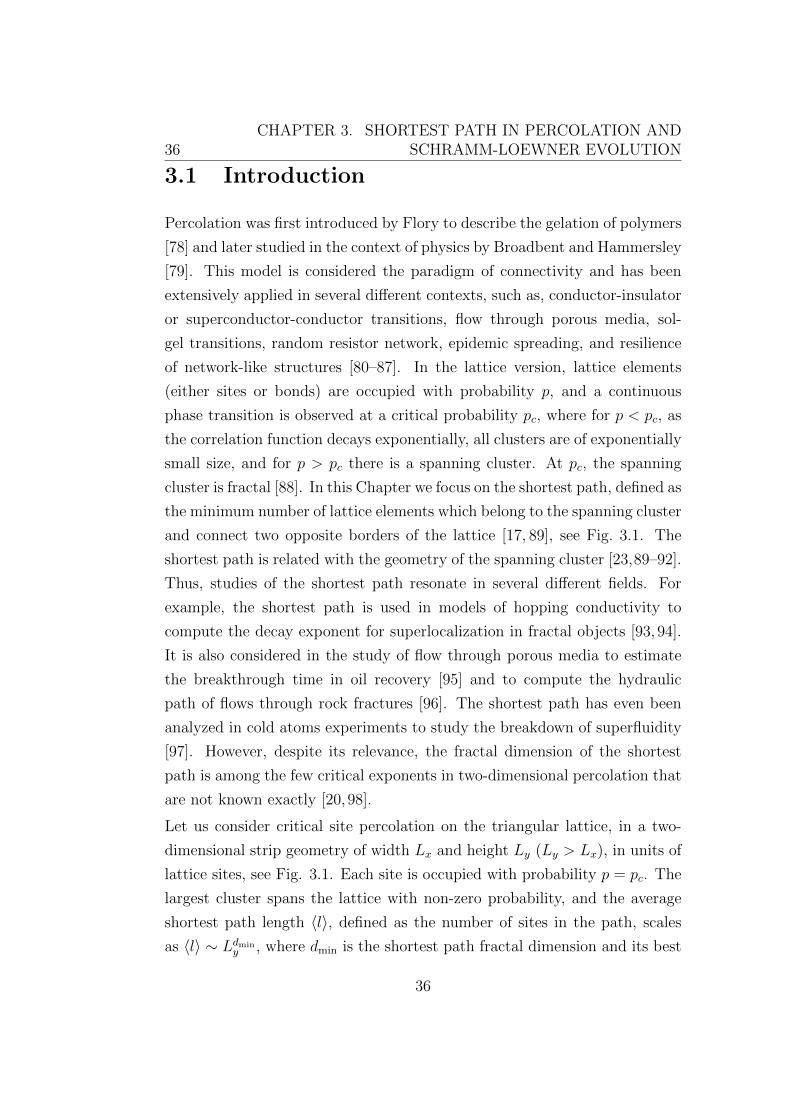
36CHAPTER 3. SHORTEST PATH IN PERCOLATION AND
SCHRAMM-LOEWNER EVOLUTION
3.1 Introduction
Percolation was first introduced by Flory to describe the gelation of polymers
[78] and later studied in the context of physics by Broadbent and Hammersley
[79]. This model is considered the paradigm of connectivity and has been
extensively applied in several different contexts, such as, conductor-insulator
or superconductor-conductor transitions, flow through porous media, sol-
gel transitions, random resistor network, epidemic spreading, and resilience
of network-like structures [80–87]. In the lattice version, lattice elements
(either sites or bonds) are occupied with probability p, and a continuous
phase transition is observed at a critical probability pc, where for p < pc, as
the correlation function decays exponentially, all clusters are of exponentially
small size, and for p > pc there is a spanning cluster. At pc, the spanning
cluster is fractal [88]. In this Chapter we focus on the shortest path, defined as
the minimum number of lattice elements which belong to the spanning cluster
and connect two opposite borders of the lattice [17, 89], see Fig. 3.1. The
shortest path is related with the geometry of the spanning cluster [23,89–92].
Thus, studies of the shortest path resonate in several different fields. For
example, the shortest path is used in models of hopping conductivity to
compute the decay exponent for superlocalization in fractal objects [93, 94].
It is also considered in the study of flow through porous media to estimate
the breakthrough time in oil recovery [95] and to compute the hydraulic
path of flows through rock fractures [96]. The shortest path has even been
analyzed in cold atoms experiments to study the breakdown of superfluidity
[97]. However, despite its relevance, the fractal dimension of the shortest
path is among the few critical exponents in two-dimensional percolation that
are not known exactly [20,98].
Let us consider critical site percolation on the triangular lattice, in a two-
dimensional strip geometry of width Lx and height Ly (Ly > Lx), in units of
lattice sites, see Fig. 3.1. Each site is occupied with probability p = pc. The
largest cluster spans the lattice with non-zero probability, and the average
shortest path length 〈l〉, defined as the number of sites in the path, scales
as 〈l〉 ∼ Ldminy , where dmin is the shortest path fractal dimension and its best
36
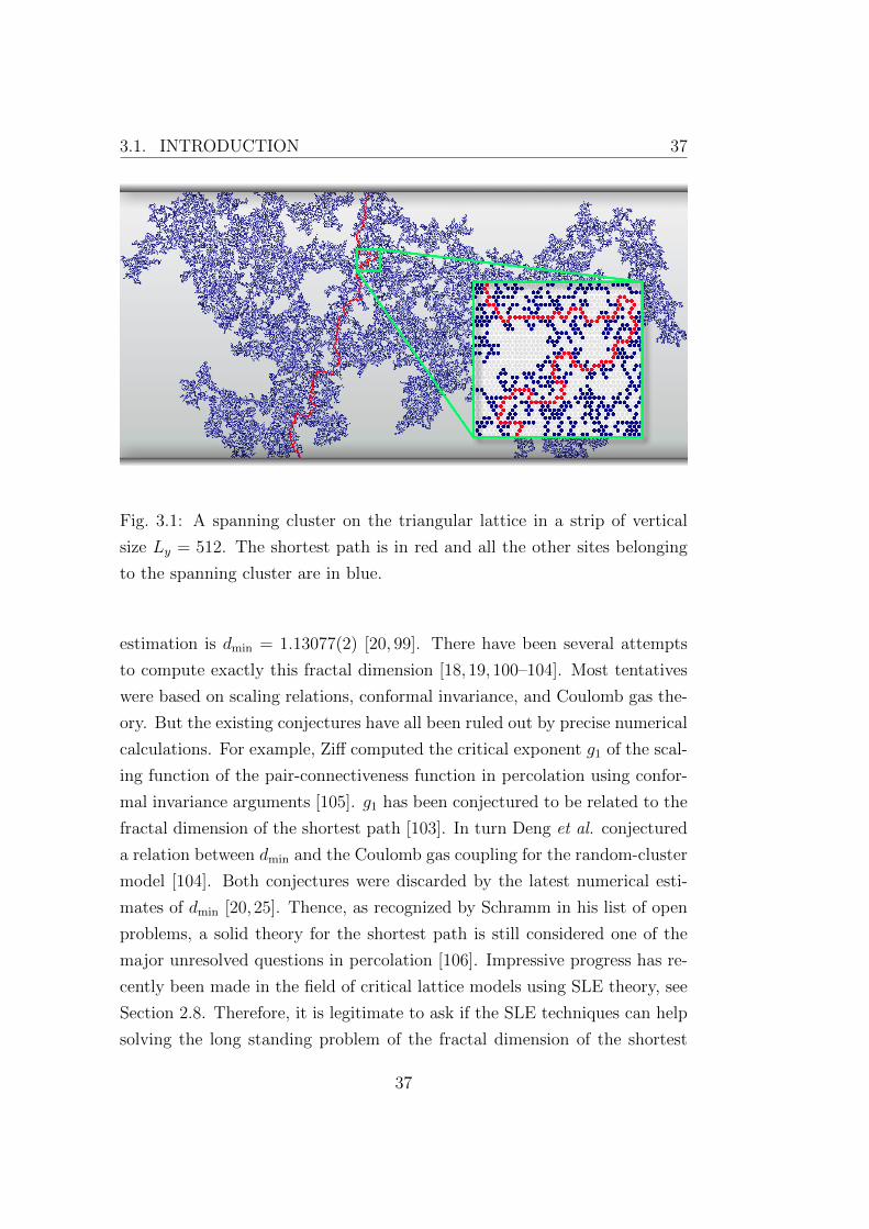
3.1. INTRODUCTION 37
Fig. 3.1: A spanning cluster on the triangular lattice in a strip of vertical
size Ly = 512. The shortest path is in red and all the other sites belonging
to the spanning cluster are in blue.
estimation is dmin = 1.13077(2) [20, 99]. There have been several attempts
to compute exactly this fractal dimension [18, 19, 100–104]. Most tentatives
were based on scaling relations, conformal invariance, and Coulomb gas the-
ory. But the existing conjectures have all been ruled out by precise numerical
calculations. For example, Ziff computed the critical exponent g1 of the scal-
ing function of the pair-connectiveness function in percolation using confor-
mal invariance arguments [105]. g1 has been conjectured to be related to the
fractal dimension of the shortest path [103]. In turn Deng et al. conjectured
a relation between dmin and the Coulomb gas coupling for the random-cluster
model [104]. Both conjectures were discarded by the latest numerical esti-
mates of dmin [20, 25]. Thence, as recognized by Schramm in his list of open
problems, a solid theory for the shortest path is still considered one of the
major unresolved questions in percolation [106]. Impressive progress has re-
cently been made in the field of critical lattice models using SLE theory, see
Section 2.8. Therefore, it is legitimate to ask if the SLE techniques can help
solving the long standing problem of the fractal dimension of the shortest
37
38CHAPTER 3. SHORTEST PATH IN PERCOLATION AND
SCHRAMM-LOEWNER EVOLUTION
path.
Also, a possible description of the physical process through SLE gives in-
teresting insights in new ways of generating the shortest path curves. Once
SLEκ is established, the value of κ suffices to generate, from only a Brow-
nian motion, curves having the same statistical properties as the shortest
path [56,107,108]. This can be very useful in the case of problems involving
optimization processes like the shortest path, watersheds [30], or spin glass
problems [57,72,73], as traditional algorithms imply the exploration of large
areas. Using the relation with SLE, even if one does not compute the curve
resulting from the optimization process for each given configuration, which
is deterministic, one is able to generate random curves, that are statistically
equivalent to the original ones, by just applying iteratively the inverse of the
uniformizing map g−1t . This leads to new ways of studying numerically and
analytically the statistical properties of complex problems.
In this article, we will show that the numerical results are consistent with
SLE predictions with κ = 1.04± 0.02. SLEκ curves have a fractal dimension
df related to κ by df = min(2, 1 + κ
8
)[52], see Section 2.7.1. From the
estimate of the fractal dimension of the shortest path, one deduces the value
of the diffusion coefficient κ corresponding to an SLE curve of same fractal
dimension; κfract = 1.0462 ± 0.0002. In what follows, we compute three
different estimates of κ using different analyses and compare them to κfract.
In particular we consider the variance of the winding angle [29,53,54], the left
passage probability [49], and the statistics of the driving function [32,57]. All
estimates are in agreement with the one predicted from the fractal dimension,
and therefore constitute a strong numerical evidence for the possibility of an
SLE description of the shortest path.
3.2 Method
We generate random site percolation configurations on a rectangular lattice
Lx×Ly with triangular mesh, where Lx and Ly are respectively the horizontal
and vertical lattice sizes, in units of lattice sites. The sites of the lattice are
38

3.3. WINDING ANGLE METHOD 39
occupied randomly with the critical probability pc = 12. If the configuration
percolates, we obtain the spanning cluster and identify the shortest path
between the top and bottom layers using a burning method [17, 82, 91]. In
short, we burn the spanning cluster from the bottom sites, indexing the sites
by the first time they have been reached, and stop the burning when we reach
for the first time the top line. We then start a second burning from the sites
on the top line that have been reached by the first burning, burning only
sites with lower index. With this procedure, we identify all shortest paths
from the bottom line to the top one. We randomly choose one of these paths,
by choosing randomly one of the starting points of the shortest path on the
bottom line, and then at each brancing of the path, choosing randomly one of
the branches. The results presented in the paper are for Ly ranging from 16
to 16384 and an aspect ratio of Lx/Ly = 1/2. We generated 10000 samples
and discarded the paths touching the vertical borders.
3.3 Winding angle method
The first result related to SLE deals with the winding angle. For each shortest
path curve we compute the variance of the winding angle, see Section 2.7.2,
and test its Gaussian statistics of variance given by Eq. (2.25)
〈θ2〉 − 〈θ〉2 = b+κ
4ln(Ly),
where b is a constant and Ly is the vertical lattice size [54]. Figure 3.2
shows the dependance of the winding angle of the shortest path on Ly in
a lin-log plot. In the inset, one shows that the distribution of the winding
angle is a Gaussian with a variance consistent with Eq. (2.25). The estimate
κwinding = 1.046 ± 0.004 that we get from fitting the data with Eq. (2.25) is
in agreement with the value deduced from the fractal dimension.
3.4 Left passage probability method
In the following, we work with chordal SLE. But the curves that we generate
with the algorithm described above are defined in a stripe starting at the
39
40CHAPTER 3. SHORTEST PATH IN PERCOLATION AND
SCHRAMM-LOEWNER EVOLUTION
0.5
1.0
1.5
2.0
101
102
103
104
<θ
2>
Ly
κ=1.046(4)
0.0
0.1
0.2
-8 -4 0 4 8
P( θ
)
θ
Fig. 3.2: Variance of the winding angle against the lattice size Ly. The
analysis has been done for Ly ranging from 16 to 16384. The statistics are
computed over 104 samples. The error bars are smaller than the symbol size.
By fitting the results with Eq. (2.25), one gets κwinding = 1.046 ± 0.004. In
the inset, the probability distribution of the winding angle along the curve is
compared to the predicted Gaussian distribution, drawn in green, of varianceκ4
ln(Ly) with κ = 1.046 and Ly = 16384.
bottom boundary and ending at the upper one, and generated with “free”
boundary conditions, i.e. without any constraints on the boundaries, such
that the shortest path has no fixed starting and ending points. Therefore we
have to map conformally the original curves into the upper half plane by an
inverse Schwarz-Christoffel transformation [50] as described in Section 2.6.
We numerically compute the left passage probability of the shortest path
curves for a given set of samples points S in the upper half-plane H and
compare the results to Schramm’s formula (2.26):
Pκ(φ) =1
2+
Γ (4/κ)√πΓ(
8−κ2κ
) cot(φ)2F1
(1
2,
4
κ,3
2,− cot(φ)2
).
We considered for convenience 400 points, regularly spaced in
[−0.1Lx, 0.1Lx] × [0.15Ly, 0.35Ly] which are then mapped through the
40
3.5. DIRECT SLE METHOD 41
inverse Schwarz-Christoffel mapping into H [50]. To estimate κ, we minimize
the weighted mean square deviation Q(κ) defined as
Q (κ) =1
|S|∑z∈S
[P (z)− Pκ(φ(z))]2
∆P (z)2,
where |S| is the cardinality of the set S, and ∆P (z)2 is defined as ∆P (z)2 =P (z)(1−P (z))
Ns−1, where Ns is the number of samples [77]. We define the error
bar ∆Q for the minimum of Q(κ) using the fourth moment of the binomial
distribution. The error ∆κ is defined such thatQ(κ±∆κ)−∆Q = Q(κ)+∆Q.
For a lattice size of Ly = 16384, the minimum of the mean square deviation
is observed for κLPP = 1.04 ± 0.02 as shown in Fig. 3.3. This value is in
agreement with the estimate of κ obtained from the fractal dimension and
the winding angle. As a remark, one might notice that the minimum of
Q deviates slightly from the expected value 1 but is of the same order of
magnitude. However one expects the SLE description of the shortest path to
be only valid in the scaling limit. The finite lattice spacing does not allow the
curve to go in all possible directions, but only in two distinct directions when
going from one site to another. Therefore, finite size effects might affect the
left-passage probability measurement and the value of the minimum of Q.
3.5 Direct SLE method
The winding angle and left passage analyses are indirect measurements of κ.
Therefore we also test the properties of the driving function directly in order
to see if it corresponds to a Brownian motion with the expected value of κ.
3.5.1 In chordal space
As for the left passage probability, we consider the chordal curves in the
upper half plane, starting at the origin and growing towards infinity. We
want to compute the driving function ξt underlying the process. For that,
we numerically solve the Loewner differential equation (2.10) using the slit
41

42CHAPTER 3. SHORTEST PATH IN PERCOLATION AND
SCHRAMM-LOEWNER EVOLUTION
3.0
4.0
5.0
6.0
1 1.02 1.04 1.06 1.08
Q
κ0
0.25
0.5
0.75
1
0 0.25 0.5 0.75 1
P(φ)
φ/π(a)
0
0.25
0.5
0.75
1
0 0.25 0.5 0.75 1
P(φ)
φ/π
-0.02
-0.01
0
0.01
0.02
0.25 0.5 0.75
P()-
P(
)
/
(b)
Fig. 3.3: Left passage probability test. (a) Weighted mean square deviation
Q(κ) as a function of κ, for Ly = 16384. The vertical blue line corresponds the
minimum ofQ(κ), and the green vertical line is a guide to the eye at κ = κfract.
The minimum of the mean square deviation is at κLPP = 1.038 ± 0.019.
The light blue area corresponds to the error bar on the value of κLPP . (b)
Computed left passage probability as a function of φ/π for R ∈ [0.70, 0.75]
and κ = 1.038. The blue line is a guide to the eye of Schramm’s formula
(2.26) for κ = 1.038.42
3.5. DIRECT SLE METHOD 43
map equation (2.29)
gt(z) = ξt +
√(z − ξt)2 + 4δt.
In the case of SLEκ the extracted driving function gives a Brownian motion
of variance κ. The direct SLE test consists in verifying that the driving
function is a Brownian motion and compute its variance 〈ξ2t 〉−〈ξt〉2 to obtain
the value of κ. The variance should behave as 〈ξ2t 〉 − 〈ξt〉2 = κt.
Figure 3.4 shows the variance of the driving function as a function of the
Loewner time t. We observe a linear scaling of the variance with t. The
local slope κdSLE(t) is shown in the inset of Fig. 3.4a. In Fig. 3.4b, we plot
the mean correlation function c(τ) = 〈c(t, τ)〉t of the increments δξt of the
driving function, where the correlation function is defined as,
c(t, τ) =〈δξt+τδξt〉 − 〈δξt+τ 〉〈δξt〉√
(〈δξ2t+τ 〉 − 〈δξt+τ 〉2) (〈δξ2
t 〉 − 〈δξt〉2). (3.1)
One sees that the correlation function vanishes after a few time steps. The
initial decay is due to the finite lattice spacing, which introduces short range
correlations. But in the continuum limit, the process is Markovian, with a
correlation function dropping immediately to zero. In the inset of Fig. 3.4b,
we show the probability distribution of the driving function for different
t. This distribution is well fitted by a Gaussian, in agreement with the
hypothesis of a Brownian driving function. From this result and the estimates
of the diffusion coefficient computed for several lattice sizes, we obtain κ =
0.9± 0.2.
We note that the numerical results obtained with the direct SLE method
are less precise than with the other analyses and, therefore, characterized by
larger error bars, as explained in Section 2.7.4. The result we have obtained
for κ is in agreement with the ones obtained with the fractal dimension,
winding angle, and left-passage probability.
3.5.2 In dipolar space
We also extracted the driving function of the curves in dipolar space, i.e.
defining the curves as starting from the origin and growing in the strip. We
43

44CHAPTER 3. SHORTEST PATH IN PERCOLATION AND
SCHRAMM-LOEWNER EVOLUTION
0
2
4
6
8
10
0.0 0.5 1.0
<ξ2
>-<
ξ>2
t
0.92
x10-3
x10-2
0.87
0.92
0.97
0.0 0.2 0.5
κd
SL
E(t
)
t
x10-2
(a)
0.0
0.2
0.4
0.6
0.8
1.0
0.0 0.5 1.0 1.5 2.0
c(τ)
τ
x10-3
g(10**(-3)*x)f(x)
10-2
10-1
100
101
-0.4 -0.2 0.0 0.2 0.4
P(ξ
t)
ξt
1.2x10⁻³
3.7x10⁻³
9.95x10⁻³
(b)
Fig. 3.4: Driving function computed using the slit map algorithm. (a) Mean
square deviation of the driving function 〈ξ2t 〉 as a function of the Loewner
time t. The diffusion coefficient κ is given by the slope of the curve. In the
inset we see the local slope κdSLE(t). The thick green line is a guide to the
eye corresponding to κdSLE = 0.92. (b) Plot of the correlation c(t, τ) given
by Eq. (3.1), and averaged over 50 time steps. The averaged value is denoted
c(τ). In the inset are shown the probability distributions of the driving
function for three different Loewner times t1 = 1.2 × 10⁻³, t2 = 3.7 × 10⁻³
and t3 = 9.95 × 10⁻³. The solid lines are guides to the eye of the form
P (ξt) = 1√2πκti
exp(− ξ2t
2κti
), for i = 1, 2, 3.
44
3.5. DIRECT SLE METHOD 45
also obtained a value of κ consistent with the fractal dimension.
Loewner’s Equation in dipolar space. Let us consider the case of a
dipolar curve growing in the strip S of height Ly, that starts at the origin
and stops the first time it hits the upper boundary. We again study the case
of simple curves. As described in Chapter 2, one expects the properties to
be the same in the strip S as in the upper half-plane H, but formulas and
especially the Loewner differential Equation (2.10) might change. Therefore
we will first develop the same formalism as in the case of chordal SLE but for
dipolar SLE leading to the Loewner differential Equation in dipolar space.
By the Riemann mapping theorem, there exist conformal maps from the strip
S minus the curve γ[0, t] into the strip S such that gt(∞) =∞ and gt(−∞) =
−∞. The map gt is then defined up to a translation by a real constant. It is
made unique by choosing the normalization limz→∞ gt(z) + gt(−z) = 0. One
parametrizes the curves such that limz→∞ gt(z)− z = t, where t is called the
Loewner time [109,110]. Dipolar SLE is defined as the collection of conformal
maps gt satisfying the following stochastic differential equation
∂gt(z)
∂t=
π/Lytanh (π (gt(z)− ξt) /2Ly)
, and g0(z) = z, (3.2)
where ξt =√κBt and Bt is a one dimensional Brownian motion starting at
the origin [109,111].
Slit map algorithm in dipolar space. Using the theory of dipolar SLE,
one can develop a numerical method to compute the driving function of
dipolar curves, as has been done in the case of chordal curves. Therefore one
has to solve Eq. (3.2). As in the chordal case, one supposes that the driving
function is constant over small time intervals δt. Under this assumption, one
can solve Eq. (3.2) and obtain the so-called slit map Equation in dipolar
space Eq. (3.3). The slit map algorithm becomes the following. Consider
a dipolar curve defined by the initial set of points {z00 , ..., z
0N}. One maps
recursively the sequence of points {zi−1i , ..., zi−1
N } of the mapped curve to the
45
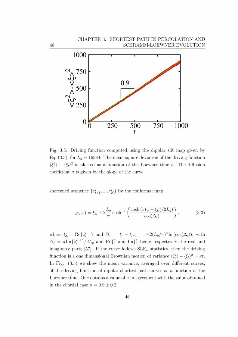
46CHAPTER 3. SHORTEST PATH IN PERCOLATION AND
SCHRAMM-LOEWNER EVOLUTION
0
250
500
750
1000
0 250 500 750 1000
<ξ2
>-<
ξ>2
t
0.9
Fig. 3.5: Driving function computed using the dipolar slit map given by
Eq. (3.3), for Ly = 16384. The mean square deviation of the driving function
〈ξ2t 〉 − 〈ξt〉2 is plotted as a function of the Loewner time t. The diffusion
coefficient κ is given by the slope of the curve.
shortened sequence {zii+1, ..., ziN} by the conformal map
gti(z) = ξti + 2Lyπ
cosh−1
(cosh (π(z − ξti)/2Ly)
cos(∆i)
), (3.3)
where ξti = Re{zi−1i } and δti = ti − ti−1 = −2(Ly/π)2 ln (cos(∆i)), with
∆i = πIm{zi−1i }/2Ly and Re{} and Im{} being respectively the real and
imaginary parts [57]. If the curve follows SLEκ statistics, then the driving
function is a one dimensional Brownian motion of variance 〈ξ2t 〉 − 〈ξt〉2 = κt.
In Fig. (3.5) we show the mean variance, averaged over different curves,
of the driving function of dipolar shortest path curves as a function of the
Loewner time. One obtains a value of κ in agreement with the value obtained
in the chordal case κ = 0.9± 0.2.
46
3.6. FINAL REMARKS 47
3.6 Final Remarks
All tests are consistent with SLE predictions. The numerical results ob-
tained with the winding angle, left-passage, and direct SLE analyses are in
agreement with the latest value of the fractal dimension. Being SLE implies
that the shortest path fulfills two properties: conformal invariance and do-
main Markov property (DMP), see Section 2.5. Thus, the agreement with
SLE predictions lends strong arguments in favor of conformal invariance and
DMP of the shortest path.
The DMP is related to the evolution of the curve in the domain of definition.
Let us consider the shortest path γ defined in a domain D, starting in a and
ending in b. We take a point c on the shortest path different from a and b.
Then if the DMP holds, one would have that
PD (γ[a, b]|γ[a, c]) = PD\γ[a,c] (γ[c, b]) , (3.4)
where γ[c, b] is the shortest path starting in c and ending in b in the domain
D except the curve γ[a, c], denoted as D \ γ[a, c], and PD and PD\γ[a,c] are the
probabilities in the domains D and D \ γ[a, c] respectively. One can classify
the models as the ones for which DMP holds already on the lattice, and the
ones for which it holds only in the scaling limit. Many classical models, like
the percolation hulls, the LERW, or the Ising model [42] for example, belong
to the first case. But some two-dimensional spin glass models with quenched
disorder [57, 73] are believed to only fulfill DMP in the scaling limit. Our
numerical results suggest that, for the shortest path, DMP holds at least in
the scaling limit. Further studies should be done to test the validity of DMP
on finite lattices.
The second result we can expect if SLE is established for the shortest path
is conformal invariance. Conformal invariance, being a powerful tool to com-
pute critical exponents, is of interest for the study of the shortest path.
Conformal invariance, associated to Coulomb gas theory for example, could
be useful to develop a field theoretical approach of the shortest path. There
is no proof of conformal invariance of the shortest path, but our numerical
results give strong support to this hypothesis. For example, the expression of
47
48CHAPTER 3. SHORTEST PATH IN PERCOLATION AND
SCHRAMM-LOEWNER EVOLUTION
the winding angle is based on conformal invariance and agrees with the pre-
dictions based on the fractal dimension. Also the left passage probabilities
and the direct SLE measurements have been performed on curves conformally
mapped to the upper half plane and gave consistent results. In addition, we
obtained the same estimate of κ by extracting the driving function in chordal
and dipolar space. However, even if the scaling limit would not be confor-
mally invariant, our results suggest that one could still apply SLE techniques
to the study of this problem, as some SLE techniques have also been used to
study off-critical and especially non conformal problems [111–115].
Analyzing the shortest path in terms of an SLE process would give a deeper
understanding of probability distributions of the shortest path, allowing to
compute more quantities, like for example the hitting probability distribution
of the shortest path on the upper boundary segment [109].
48
Chapter 4
Long-range correlated
landscapes and correlated
percolation
In the previous chapter, we have studied the shortest path in usual perco-
lation, where each site is occupied randomly with a given probability pc,
independently of the state, empty or occupied, of the other sites. In the fol-
lowing we will be interested in the properties of correlated percolation, where
the state of each cell is not independent from the state of the others. Actually
correlated percolation can be related to long-range correlated landscapes in
the framework of ranked surfaces introduced recently in the work of Schrenk
et al. [116].
Since the seminal paper of Mandelbrot [117], real and artificial landscapes
have gained much interest [12,118]. Physicists have been especially interested
in the self-affine properties of random surfaces, in the fractal dimension of
their isoheight lines, and their critical properties. Landscapes can describe
several properties such as topography [119], energy [120], temperature [33]
or vorticity fields [32]. They have been employed in the study of water
basins [30, 121–125], electronic transport [120], deposition of particles on
layers [37,126,127] and turbulence [32,33]. Landscapes are characterized by
the so-called Hurst exponent. The features of the physical system are then
intimately connected to the properties of the landscape. In the following, we
49

50CHAPTER 4. LONG-RANGE CORRELATED LANDSCAPES AND
CORRELATED PERCOLATION
will define correlated percolation in the framework of ranked surfaces, study
the characterization of these surfaces and present a method to generate long-
range correlated surfaces.
4.1 Correlated percolation
To study correlated percolation on a lattice, we work with a landscape of ran-
dom heights h, where h(x) is the height of the landscape at position x in the
lattice [14,22,27,118,128,129]. One then constructs the ranked surface [116]
associated to this discrete landscape. It is constructed as follows: one first
ranks all sites in the landscape according to their height, from the smallest
to the largest value. Then the ranked surface is constructed by assigning
to each site a number corresponding to its position in the rank. One then
floods the landscape starting from the lowest to the heighest rank. A frac-
tion p of sites is flooded. If one considers the height hc of the last occupied
site, then the problem is equivalent to the one where one floods the land-
scape till height hc. As developed by Ziman and Weinrib [120, 130], there is
a simple mapping between correlated percolation and random surfaces with
−1 ≤ H < 0, where H is the Hurst exponent related to the height-height
correlation function through
c(r) = 〈h(x)h(x + r)〉x ∼ |r|2H . (4.1)
By identifying for example the sites above hc as occupied and the sites be-
low hc as empty, one can map this problem to a percolation problem with
occupation probability 1 − p. For example, if the heights are distributed
uniformly at random, classical percolation with a fraction of occupied sites
1−p is obtained [2,3]. In the case of long-range correlated percolation, there
exists a critical height hc or critical occupation probability pc, at which a
global connectivity appears in the system [99].
In the context of percolation, one will mostly speak about boundary of perco-
lation clusters, focusing on the occupation probability, whereas in the context
of SLE, one mostly speaks of isoheight lines at a critical height hc, but the
two problems are related, see Fig. 4.1.
50
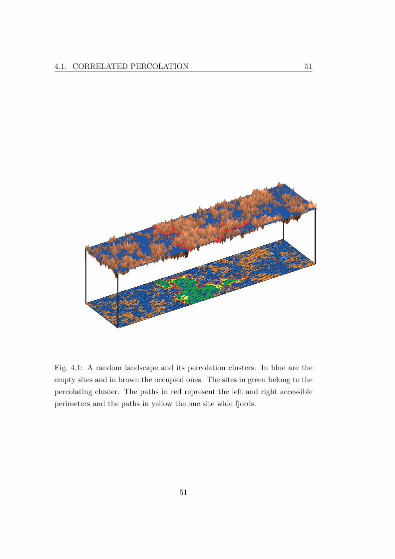
4.1. CORRELATED PERCOLATION 51
Fig. 4.1: A random landscape and its percolation clusters. In blue are the
empty sites and in brown the occupied ones. The sites in green belong to the
percolating cluster. The paths in red represent the left and right accessible
perimeters and the paths in yellow the one site wide fjords.
51
52CHAPTER 4. LONG-RANGE CORRELATED LANDSCAPES AND
CORRELATED PERCOLATION
4.2 The Hurst exponent of long-range corre-
lated landscapes
Let us consider random surfaces, i.e. a function that returns to each grid
point (x, y) in a lattice the corresponding random height h(x, y) = h(x).
They are parametrized by the so-called Hurst exponent H, and their statis-
tical properties depend on H.
The most general way to characterize the Hurst exponent of a given surface
is through its power-spectrum that is related to the Fourier transform of the
surface. It is defined as,
S(q) =1
(2π)2 |〈h(r)e−iq·r〉r|2 (4.2)
and is expected to scale as
S(q) ∼ |q|−2(H+1), (4.3)
where H is the Hurst exponent. In the following, we will be interested in
the cases H ∈ [−1, 0) and H ∈ (0, 1]. By the Wiener-Khintchine theorem
[131,132], this definition translates into scaling relations for the height-height
correlation function [14].
One usually considers the scaling of the height-height correlation function
c(r) = 〈h(x)h(x + r)〉x ∼ a(H) + b(H)|r|2H . (4.4)
For −1 < H < 0, one considers the decrease of the height-height correlation
function for large values of |r|, with a(H) = 0 and b(H) > 0 in Eq. (4.4),
see Eq. (4.1). Weinrib proposed to use these surfaces to develop the so-
called long-range correlated percolation framework, where the formalism of
percolation is applied [118,128].
In the case 0 < H < 1, one considers the decrease of the height-height
correlation function for small values of |r|, with a(H) > 0 and b(H) < 0
in Eq. (4.4). These surfaces with 0 < H < 1 are sometimes called rough
52

4.3. THE FOURIER FILTERING METHOD FOR CORRELATEDLANDSCAPES 53
surfaces, andH is called the roughness exponent. In particular, these surfaces
are self-affine [133] and their height profiles are scale invariant [134]
h(εx) ∼ εHh(x). (4.5)
Surfaces with values of H next to one are “smoother” than surfaces with
values of H next to zero, which look more rough1.
Rough self-affine surfaces [136], i.e. surfaces with Hurst exponent H ∈ (0, 1],
have been the object of many theoretical [12, 27] and experimental studies,
and have triggered the development of many models [126,127,137]. Most of
the real landscapes one encounters in nature have postive Hurst exponent.
Random surfaces with negative Hurst exponent, H ∈ [−1, 0), have been
studied in relation to correlated percolation [22,128,129,138,139].
4.3 The Fourier Filtering Method for corre-
lated landscapes
The simplest landscapes one can think of are uncorrelated landscapes, where
the height of each site is chosen uniformly at random. But real landscapes
are correlated and the heights typically are long-range correlated. There-
fore specific methods were developed to generate rough surfaces exhibiting
correlations. For example, growth models have been developed, like con-
tinuous growth models in the cases of the Edward-Wilkinson [126] and the
Kardar-Parisi-Zhang [127] models, and discrete growth models in the cases
of ballistic deposition [140] and Solid-On-Solid models [141]. Here we will
present one method to generate random surfaces, called the Fourier Filtering
Method, and present its relation to Gaussian random fields.
1In many real surfaces, there exists a correlation length ξ and the surface will
exhibit self-affinity only on a length scale smaller than the correlation length. In
this case one might write the height-height correlation function in the form H(r) =
w2
[1− exp
(−(|r|ξ
)2H)], which corresponds to an exponential decrease of the auto-
correlation function. Also the scaling law is expected to be valid for |q| >> ξ−1 [135].
53
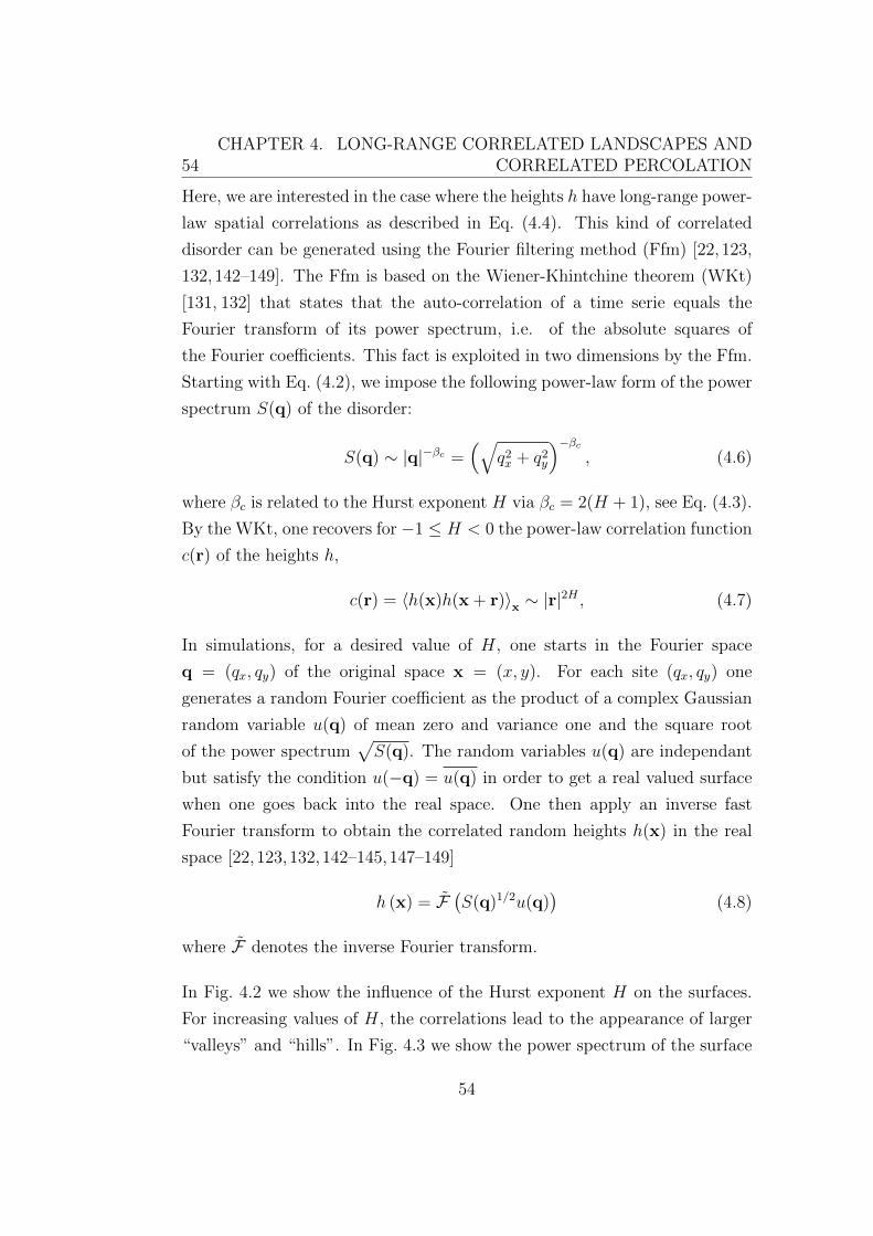
54CHAPTER 4. LONG-RANGE CORRELATED LANDSCAPES AND
CORRELATED PERCOLATION
Here, we are interested in the case where the heights h have long-range power-
law spatial correlations as described in Eq. (4.4). This kind of correlated
disorder can be generated using the Fourier filtering method (Ffm) [22, 123,
132, 142–149]. The Ffm is based on the Wiener-Khintchine theorem (WKt)
[131, 132] that states that the auto-correlation of a time serie equals the
Fourier transform of its power spectrum, i.e. of the absolute squares of
the Fourier coefficients. This fact is exploited in two dimensions by the Ffm.
Starting with Eq. (4.2), we impose the following power-law form of the power
spectrum S(q) of the disorder:
S(q) ∼ |q|−βc =(√
q2x + q2
y
)−βc, (4.6)
where βc is related to the Hurst exponent H via βc = 2(H + 1), see Eq. (4.3).
By the WKt, one recovers for −1 ≤ H < 0 the power-law correlation function
c(r) of the heights h,
c(r) = 〈h(x)h(x + r)〉x ∼ |r|2H , (4.7)
In simulations, for a desired value of H, one starts in the Fourier space
q = (qx, qy) of the original space x = (x, y). For each site (qx, qy) one
generates a random Fourier coefficient as the product of a complex Gaussian
random variable u(q) of mean zero and variance one and the square root
of the power spectrum√S(q). The random variables u(q) are independant
but satisfy the condition u(−q) = u(q) in order to get a real valued surface
when one goes back into the real space. One then apply an inverse fast
Fourier transform to obtain the correlated random heights h(x) in the real
space [22,123,132,142–145,147–149]
h (x) = F(S(q)1/2u(q)
)(4.8)
where F denotes the inverse Fourier transform.
In Fig. 4.2 we show the influence of the Hurst exponent H on the surfaces.
For increasing values of H, the correlations lead to the appearance of larger
“valleys” and “hills”. In Fig. 4.3 we show the power spectrum of the surface
54
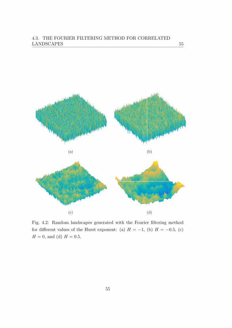
4.3. THE FOURIER FILTERING METHOD FOR CORRELATEDLANDSCAPES 55
(a) (b)
(c) (d)
Fig. 4.2: Random landscapes generated with the Fourier filtering method
for different values of the Hurst exponent: (a) H = −1, (b) H = −0.5, (c)
H = 0, and (d) H = 0.5.
55
56CHAPTER 4. LONG-RANGE CORRELATED LANDSCAPES AND
CORRELATED PERCOLATION
jqj100 101 102 103
Sjq
j
10-4
10-3
10-2
10-1
100
(a)
qx
1 256 512
q y
1
256
512
-3
-2
-1
0
1
2
3
(b)
Fig. 4.3: Properites of the Fourier transform of one random landscape of
Hurst exponent H = −0.5 generated with the Fourier Filtering Method.
(a) Power spectrum Sq = |h(q)|2 as a function of |q|, where h is the Fourier
transform of the surface h. The red line is a guide to the eye of the form |q|−βc
with βc = 2(H + 1). (b) Phase φ = arg(h(q)) as a function of q = (qx, qy).
56
4.4. CORRELATED SURFACES, FOURIER FILTERING METHODAND FRACTIONAL GAUSSIAN FIELDS 57
generated with the Fourier filtering method and the phase of its Fourier
components. The phases are uniformly random in (−π, π].
In the following, we will be especially interested in the range −1 ≤ H ≤ 0,
that is related to correlated percolation [22,118,128,129]. The case H = −1
corresponding to βc = 0 is such that the power spectrum in Eq. (4.6) is in-
dependent on the frequency, and the landscape profile is white noise. Since
H ≤ 0, as H increases towards zero, the correlation function decays more
slowly. For H = 0 one recovers the Gaussian Free Field (GFF) [150].
The discrete Gaussian Free Field Γ is a centered Gaussian random vector,
whose covariance matrix is the Green’s function of the random walk, i.e.
E(Γ(x)Γ(y)) = GD(x, y), where GD(x, y) is the Green’s function of the ran-
dom walk in the domain D [151]. It is defined as the mean number of times
a random walker (Xn)n≥0 starting at x spends at y before it exits the domain
D, i.e. GD(x, y) = Ex(∑τ−1
n=0 1Xn=y), where τ is the first exit time of D of the
random walker (Xn)n≥0, the index x in Ex indicating that the random walker
starts at x. Actually, GD(x, y) is symmetric in x and y, and is an admissible
covariance matrix, see [151]. It is also the Green’s function of the Laplacian
operator, see [151], and Section 4.4.
4.4 Correlated surfaces, Fourier Filtering
Method and fractional Gaussian fields
In this section we draw a parallel between random surfaces generated with the
Fourier filtering method and the mathematical theory of fractional Gaussian
fields that could be of interest to tackle long-range correlated percolation
theory from an analytical point of view. Here we do not enter in mathematical
details, but for rigorous proofs, the reader can refer to Refs. [39,150].
One can generalize the results obtained for the Gaussian Free Field, asso-
ciated to a Laplacian operator [150], to the so-called Fractional Gaussian
Fields (FGF) [39], associated to fractional Laplacians. The fractional Lapla-
cian is parametrized by a real valued parameter s, that plays a similar role
57
58CHAPTER 4. LONG-RANGE CORRELATED LANDSCAPES AND
CORRELATED PERCOLATION
to H in the case we studied before. For long-range correlated percolation,
we are interested in the range s ∈ (0, 1), see below. The fractional Lapla-
cian for s ∈ (0, 1) is defined such that the eigenvectors of the fractional
Laplacian are the eigenvectors of the Laplacian with Dirichlet boundary con-
ditions. If (λn, fn) are the eigenvalues and eigenfunctions of the Laplace
operator with Dirichlet boundary conditions, then (λs/2n , fn) are the eigenval-
ues and eigenfunctions of the fractional Laplacian operator and the functions
(λ−s/2n fn) form an othonormal basis associated to an inner product related to
the fractional Laplacian (see [39] and especially section 9 on the eigenfunc-
tion FGF). But on the unit torus, see [150] paragraph 2.5, the eigenfunctions
of the Dirichlet Laplace operator are x 7→ e2πix.k with eigenvalues (2π|k|)2
and k ∈ Z2 \ {0}. Therefore using H = s− 1, one obtains that the functions
x 7→ 1(2π|k|)s e
2πix.k are an othornomal basis for the inner product associated
to the fractional Laplacian. By proposition 2.1 point 2 of [150], multiplying
each of these components by a Gaussian random variable uk, one obtains that
h(x) =∑
k uk(2π|k|)−se2πix.k is a Gaussian random variable with probability
measure µV = e−(v,v)∇sZ−1dv, where (. , . )∇s is the inner product associated
to the fractional Laplacian and Z is a normalizing constant. For a compar-
ison between the case of the GFF and the FGF, see [39] paragraph 12.2.
Using the relation s = βc/2 in the case of a lattice with periodic boundary
conditions one recovers the random function defined in the Fourier filtering
method, up to a multiplicative constant (2π)s−1/2.
One might also approach the problem in real space. We define in R2 the
function valued fractional gradient
∇sf(x) =
(y 7→ f(x+ y)− f(x)
|y|1+s
), (4.9)
and the real valued fractional Laplacian
(−∆)sf(x) =
∫R2
f(x+ y)− 2f(x) + f(x− y)
|y|2+2sdy, (4.10)
see [39] paragraph 12. These formulas are defined up to normalization con-
stants, see Proposition 2.2 in [39]. Actually, the easiest way to defined the
58
4.4. CORRELATED SURFACES, FOURIER FILTERING METHODAND FRACTIONAL GAUSSIAN FIELDS 59
fractional Laplacian is by generalizing the usual derivation expressed using
the Fourier Transform. If (−∆)sg = h, then the Fourier transforms f , g
satisfy f(k) = |k|2sg(k).
One defines the inner product (. , . )∇s as
(f, g)∇s =
∫R2
(∇sf(x),∇sg(x)) dx (4.11)
and shows that it is equal to∫R2
(∇sf(x),∇sg(x)) dx =
∫R2
((−∆)sf(x))g(x)dx,
(f, g)∇s = ((−∆)sf, g),
(4.12)
see [39] proposition 12.1, where (·, ·) denotes the usual L2 inner product in
R2, i.e. (f, g) =∫R2 f(x)g(x)dx.
The covariance follows the expected scaling relation, see Eq. (4.7), i.e. scales
as |r|2H , cf. Theorem 3.3 in [39].
From this we see that the main difference between the cases H = 0 and
H ∈ (−1, 0), is that the random landscapes that we generate with the Fourier
filtering method are not related to a local operator anymore, the Laplacian,
but to a long-range operator, the fractional Laplacian operator (−∆)s.
This formalism is especially usefull if one wants to simulate long-range corre-
lated random fields in a domain D with fixed boundary conditions f |∂D. In
order to do so, one generates a Gaussian random field h(x) using the Fourier
filtering method. Then one computes the deterministic correction field h(x)
as the solution of:
(−∆)βc/2h = 0,
and h|∂D = f |∂D − h|∂D.(4.13)
Then the long-range correlated landscape hfinal in D with fixed boundary
conditions f |∂D is defined as:
hfinal(x) = h(x) + h(x), (4.14)
for x ∈ D.
59
60CHAPTER 4. LONG-RANGE CORRELATED LANDSCAPES AND
CORRELATED PERCOLATION
Intuitively, if one computes (hfinal, hfinal)∇s with s = βc/2, by Eq. (4.12)
one gets that (hfinal, hfinal)∇s = (h, h)∇s + 2(h, h)∇s + (h, h)∇s = (h, h)∇s +
2((−∆)sh, h) + ((−∆)sh, h) = (h, h)∇s . Therefore the inner product, and as
a consequence the probability distribution, is not changed. For more details,
see [35] and Section 5 of [39].
Using this method, one generates long-range correlated Gaussian fields with
fixed boundary conditions and the desired probability density, see Fig. 4.4.
Fixing the boundary conditions might play a role in SLE studies, see for
example Ref. [35].
60

4.4. CORRELATED SURFACES, FOURIER FILTERING METHODAND FRACTIONAL GAUSSIAN FIELDS 61
3530
2520
x15
105
00
5
10
15
20
y
25
30
0
10
20
30
40
35
z
(a)
3530
2520
x15
105
00
5
10
15
20
y
25
30
20
0
-20
-40
-60
-8035
z
(b)
Fig. 4.4: Generating long range correlated surfaces with fixed
boundary conditions. Square surface of lattice size L = 32 and Hurst
exponent H = −0.1. The boundary conditions are L on one half of the
boundary and −L on the other half. (a) Random surface h(x) generated
with free boundary counditions. (b) Correction field h satisfying the bound-
ary value problem Eq. (4.13).
61
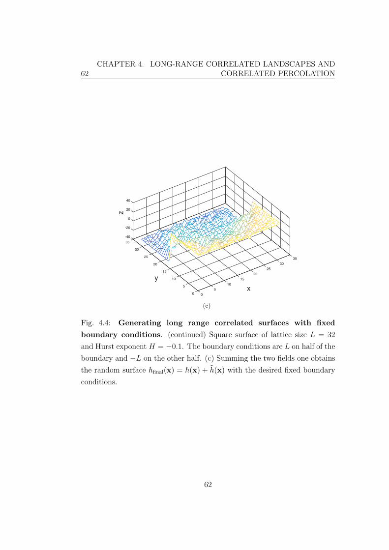
62CHAPTER 4. LONG-RANGE CORRELATED LANDSCAPES AND
CORRELATED PERCOLATION
3530
2520
x15
105
00
5
10
15
20
y
25
30
-40
-20
0
20
40
35
z
(c)
Fig. 4.4: Generating long range correlated surfaces with fixed
boundary conditions. (continued) Square surface of lattice size L = 32
and Hurst exponent H = −0.1. The boundary conditions are L on half of the
boundary and −L on the other half. (c) Summing the two fields one obtains
the random surface hfinal(x) = h(x) + h(x) with the desired fixed boundary
conditions.
62

Chapter 5
Long-range correlated
percolation
As we have seen in Chapter 4, and especially in Fig. 4.2, the long-range corre-
lations change the topography of the landscapes and therefore the percolation
properties associated to these surfaces.
In this Chapter, we investigate quantitatively, using Monte-Carlo simula-
tions, the influence of the power-law correlation of the site occupation proba-
bilities on the long-range correlated percolation problem. We compute several
critical exponents as function of the Hurst exponent H which characterizes
the spatial correlations among the occupation of sites as described in Sec-
tion 4.2. In particular, we study the fractal dimension of the largest cluster
and of its complete and accessible perimeters. We also discuss the cluster
size distribution at criticality. Concerning the inner structure and transport
properties of the largest cluster, we analyze its shortest path, backbone, and
cluster conductivity. We propose expressions for the functional dependence
of the critical exponents associated to these quantities on the Hurst exponent
H.
This chapter is based on Ref. [99]:
K. J. Schrenk, N. Pose, J. J. Kranz, L. V. M. van Kessenich, N. A. M.
Araujo and H. J. Herrmann, Percolation with long-range correlated disorder,
Physical Review E 88, 052102 (2013).
63
64 CHAPTER 5. LONG-RANGE CORRELATED PERCOLATION
5.1 Introduction
Percolation theory and related models have been applied to study trans-
port and geometrical properties of disordered systems [118,152] as described
in Section 3.1. Frequently the disorder in the system under study exhibits
power-law long-range spatial correlations. This fact has motivated some
studies of percolation models where the sites of the lattice are not occupied
independently, but with some correlation between the occupation probabili-
ties, leading to correlated percolation as described in Section 5.2. As one can
guess from Fig. 4.2 and from previous work [22,118,128,129,139,146,152–159],
in the presence of long-range correlations, percolation clusters become more
compact and their transport properties change accordingly.
The critical exponents for uncorrelated percolation in two dimensions are
known rigorously for the triangular lattice [63]. In addition, at the critical
point, the correlation-length diverges and universality holds, i.e., critical ex-
ponents and amplitude ratios do not depend on short-range details, such as
lattice specifics [82, 83, 88, 118, 152]. This statement has been made precise
by renormalization group theory, which predicts that the scaling functions
within a universality class are the same, while the lattice structure only in-
fluences the non-universal metric factors [160, 161]. If, by contrast, infinite-
range, power-law correlations are present, according to the extended Harris
criterion, the critical exponents can change, depending on how the correla-
tions decay with spatial distance [128,129,146,162,163].
In this Chapter, we investigate a two-dimensional percolation model where
the sites of a lattice are occupied based on power-law correlated disorder, see
Section 4.1, parametrized by the Hurst exponent H and generated with the
Fourier filtering method, see Section 4.3. We find that the fractal dimension
of the largest cluster, its complete and accessible perimeters, as well as the
dimension of its shortest path depend on H. Strong dependence on H is
also found for the fractal dimension of the backbone and the electrical con-
ductivity exponent. For two-dimensional critical phenomena, conformal field
theory has been used to obtain exact values of critical exponents in the form
of simple rational numbers [164–166]. Therefore, we make proposals for the
64

5.2. CORRELATED PERCOLATION AND THE EXTENDED HARRISCRITERION 65
functional dependence of all measured exponents on the Hurst exponent H,
as being the simplest rational expressions that fit the numerical data.
In Sec. 5.2, we discuss the influence of the long-range correlations on the
percolation problem in terms of the extended Harris criterion. In Sec. 5.3,
we study the percolation threshold of the used lattice. In Sec. 5.4 we measure
the fractal dimension of the largest cluster and the cluster size distribution at
the percolation threshold. In Sec. 5.5 the complete and accessible perimeters
of the largest cluster are investigated. Section 5.6 discusses the shortest path
of the largest cluster, its backbone and cluster conductivity at the percolation
threshold. Finally, in Sec. 5.7, we present some concluding remarks.
5.2 Correlated percolation and the extended
Harris criterion
In correlated percolation, the usual uncorrelated percolation model is mod-
ified by long-range correlations of the occupation probabilities. One might
wonder if the correlations are strong enough to change the critical behav-
ior of the system. For short-range correlated systems, the Harris criterion
states that short-range correlations are relevant if dν − 2 < 0 [167]. As this
is always positive for percolation, short-range correlations have no influence
on the critical behavior of percolation. But this is not always the case for
long-range power-law correlations, for which the Harris criterion has been
extended. In a system of lateral size L, where the control parameter is the
height h of the landscape, for −1 ≤ H < 0, the height-height correlation
function looks like c(r) ∼ |r|2H , as described in Section 4.1 discussing the re-
lation between correlated landscapes and correlated percolation. Therefore
if one considers a lattice of size L at criticality, the correlation length ξ scales
as ξ ∼ L. Therefore if one considers the variance of the mean value of the
heights ∆2 = 〈[1/ξ2
∫ξ×ξ dxh(x)
]2
〉, where the average is over the disorder
65
66 CHAPTER 5. LONG-RANGE CORRELATED PERCOLATION
realisations, in a square of lateral size ξ, then it scales as:
〈[1/ξ2
∫ξ×ξ
dxh(x)
]2
〉 = 1/ξ4
∫(ξ×ξ)2
dxdy〈h(x)h(y)〉,
∆2 ∼ 1/ξ2
∫ ξ
0
c(r)rdr,
∆2 ∼ ξ2H ,
∆2 ∼ L2H .
(5.1)
But by definition of the correlation length critical exponent L ∼ ξ ∼|h∗ − hc|−νuncorr , where h∗ is the effective critical height, hc is the infinite
size critical height, and νuncorr the correlation-length critical exponent in 2D
in the uncorrelated case. The effect of the long-range correlations is neg-
ligeable in the thermodynamic limit if the local fluctuations of the control
parameter due to the long-range correlations are small compared to the dis-
tance to the critical point. Therefore the effect of the long-range correlations
is negligeable in the thermodynamic limit if ∆2/|h∗−hc|2 ∼ L2H+2/νuncorr → 0
when L→∞, leading to H < −1/νuncorr.
Therefore, the extended Harris criterion, as formulated in Refs. [128, 129,
146, 162, 163], states that for the range −d/2 < H < 0 the correlations
do not affect the critical exponents of the percolation transition if H ≤−1/νuncorr, where νuncorr is the correlation-length critical exponent and for
d = 2, νuncorr2D = 4/3 [63,82]. Whereas for −1/νuncorr
2D < H < 0 the critical ex-
ponents are expected to depend on the value of H. The quantitative depen-
dence of the critical exponents on H, in this regime, is not yet entirely clear.
Concerning the correlation-length critical exponent for the correlated case
νH , the analytical works in Refs. [128, 129, 162] predict that νH = −1/H.
In the case of Weinrib and Halperin [128, 162] this is a conjecture based
on renormalization group calculations; Schmittbuhl et al. [129] found the
same result by analyzing hierarchical networks. Therefore, in both analyti-
cal approaches, it is not certain that νH actually behaves as conjectured and
there is some controversy regarding this question, as discussed, e.g., in the
field-theoretical work of Prudnikov et al. [168, 169]. For correlated percola-
tion, the relation νH = −1/H has been supported by the numerical work in
66
5.3. PERCOLATION THRESHOLD 67
Refs. [146,170,171]. Agreement has also been reported by Prakash et al. [22],
however only approximately for the range −1/νuncorr2D ≤ H ≤ −0.5. Finally,
for H > 0 there is no percolation transition [129, 172]. In the following, we
consider values of the Hurst exponent in the range −1 ≤ H ≤ 0.
5.3 Percolation threshold
We consider the correlated percolation model defined in Section 4.1 on tri-
angular lattice stripes of vertical length Ly = L and aspect ratio A = Lx/Ly,
consisting of N = AL2 sites. To investigate critical correlated percolation,
one first needs to identify the percolation threshold pc, which is pc = 1/2 for
site percolation on the triangular lattice [82]. To compute the percolation
threshold of a percolation problem on a given lattice, one can find their cor-
responding matching lattice. The most visual explanation of the concept of
matching lattice is the following [118]: Suppose that for a lattice G1 there ex-
ists a different lattice G2, such that each site in lattice G1 is uniquely related
to one site in G2 and the other way around. Also, assume that if a site is oc-
cupied in one of the lattices, its partner in the other one can not be occupied.
Now, if the presence of a cluster spanning G2 in one direction prevents any
cluster spanning G1 in the perpendicular direction and, conversely, there can
only be a percolating cluster in G1 if there is no percolation in G2, then G1
and G2 are matching lattices. For example, the triangular lattice is its own
matching lattice, called self-matching, while the square lattice is matched by
the star lattice [173]. Sykes and Essam argued, based on the uniqueness of
the threshold pc [173–175], that for any lattice G1 and its matching one G2,
the sum of the thresholds of both equals unity:
pG1c + pG2
c = 1. (5.2)
Then, since the triangular lattice is self-matching, one has pG1c = pG2
c and it
follows that pc = 1/2. The question of which pairs of lattices match each
other is independent on the statistical properties of the heights h that deter-
mine the cluster properties. Therefore, the site percolation threshold of the
triangular lattice is pc = 1/2, also for correlated percolation. We also checked
67

68 CHAPTER 5. LONG-RANGE CORRELATED PERCOLATION
10-4
10-3
10-2
10-1
101
102
103
104
p
c,J
−pc
Lattice size L
0.75±0.02
0.73±0.03
0.68±0.05
0.41±0.05
0.13±0.05
-1
-0.85
-0.7
-0.4
-0.1
Fig. 5.1: Convergence of the percolation threshold estimator pc,J . The differ-
ence between the estimator and the threshold |pc,J − 1/2| is shown as function
of the lattice size L for H = −1, H = −0.85, −0.7, −0.4, and −0.1. The
data is shifted vertically to improve visibility. Results are averages over at
least 104 samples. We keep track of the cluster properties with the labeling
method proposed by Newman and Ziff [2, 3], as in Ref. [4].
this statement numerically by measuring pc for different values of the Hurst
exponent H, finding that it is compatible with 1/2, within error bars.
As a first check of the theory presented in Refs. [128,129,162] regarding the
dependence of νH on H, we consider here the convergence of a threshold
estimator, namely the value pc,J at which the maximum change in the size
of the largest cluster smax occurs [176–183]. The expected scaling behavior
[99,178] is
|pc,J(L)− pc| ∼ L−1/νH , (5.3)
where pc = 1/2. Figure 5.1 shows |pc,J(L)− pc| as function of the lattice size
L for different values of H. Within error bars, the data is compatible with
1/νH = −H for the considered values of H.
68
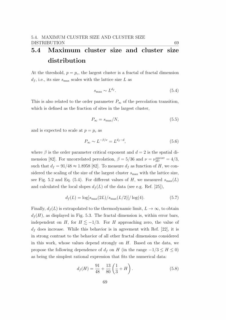
5.4. MAXIMUM CLUSTER SIZE AND CLUSTER SIZEDISTRIBUTION 69
5.4 Maximum cluster size and cluster size
distribution
At the threshold, p = pc, the largest cluster is a fractal of fractal dimension
df , i.e., its size smax scales with the lattice size L as
smax ∼ Ldf . (5.4)
This is also related to the order parameter P∞ of the percolation transition,
which is defined as the fraction of sites in the largest cluster,
P∞ = smax/N, (5.5)
and is expected to scale at p = pc as
P∞ ∼ L−β/ν = Ldf−d, (5.6)
where β is the order parameter critical exponent and d = 2 is the spatial di-
mension [82]. For uncorrelated percolation, β = 5/36 and ν = νuncorr2D = 4/3,
such that df = 91/48 ≈ 1.8958 [82]. To measure df as function of H, we con-
sidered the scaling of the size of the largest cluster smax with the lattice size,
see Fig. 5.2 and Eq. (5.4). For different values of H, we measured smax(L)
and calculated the local slopes df (L) of the data (see e.g. Ref. [25]),
df (L) = log[smax(2L)/smax(L/2)]/ log(4). (5.7)
Finally, df (L) is extrapolated to the thermodynamic limit, L→∞, to obtain
df (H), as displayed in Fig. 5.3. The fractal dimension is, within error bars,
independent on H, for H . −1/3. For H approaching zero, the value of
df does increase. While this behavior is in agreement with Ref. [22], it is
in strong contrast to the behavior of all other fractal dimensions considered
in this work, whose values depend strongly on H. Based on the data, we
propose the following dependence of df on H (in the range −1/3 ≤ H ≤ 0)
as being the simplest rational expression that fits the numerical data:
df (H) =91
48+
13
80
(1
3+H
). (5.8)
69
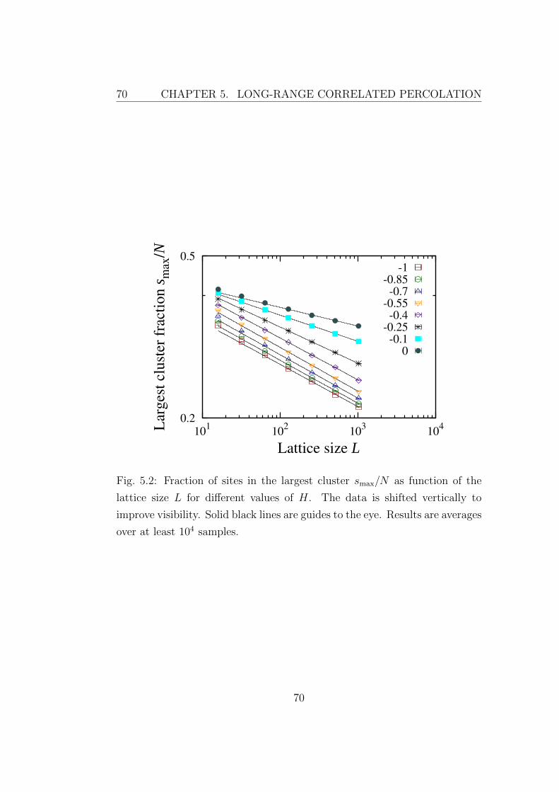
70 CHAPTER 5. LONG-RANGE CORRELATED PERCOLATION
0.2
0.5
101
102
103
104L
arg
est
clu
ster
fra
ctio
n s
max
/N
Lattice size L
-1-0.85-0.7
-0.55-0.4
-0.25-0.1
0
Fig. 5.2: Fraction of sites in the largest cluster smax/N as function of the
lattice size L for different values of H. The data is shifted vertically to
improve visibility. Solid black lines are guides to the eye. Results are averages
over at least 104 samples.
70
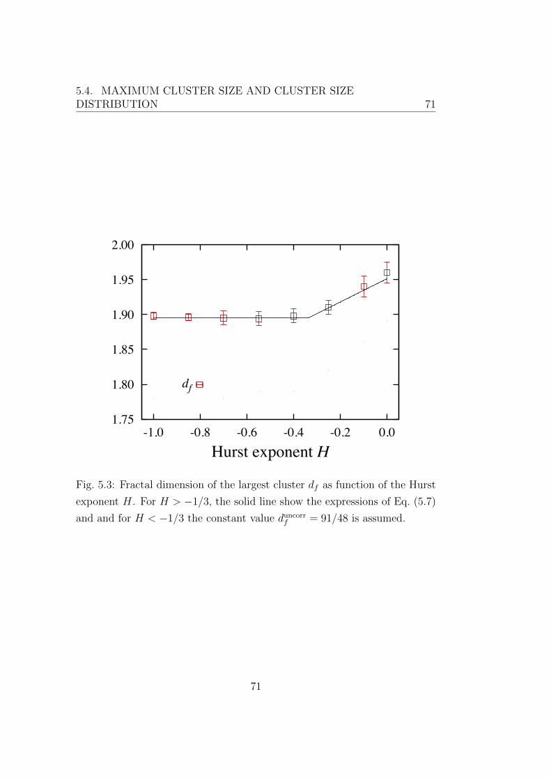
5.4. MAXIMUM CLUSTER SIZE AND CLUSTER SIZEDISTRIBUTION 71
1.75
1.80
1.85
1.90
1.95
2.00
-1.0 -0.8 -0.6 -0.4 -0.2 0.0Hurst exponent H
df
Fig. 5.3: Fractal dimension of the largest cluster df as function of the Hurst
exponent H. For H > −1/3, the solid line show the expressions of Eq. (5.7)
and and for H < −1/3 the constant value duncorrf = 91/48 is assumed.
71

72 CHAPTER 5. LONG-RANGE CORRELATED PERCOLATION
10-8
10-4
100
104
108
101
102
103
104
105
106
107
Clu
ste
r siz
e n
s
Lattice size L
-1
-0.85
-0.7
-0.55
-0.4
-0.25
-0.1
0
Fig. 5.4: Cluster size distribution ns as a function of the number of occupied
sites s, for different values of the Hurst exponent H. The data is shifted
vertically to improve visibility. Solid black lines are guides to the eye. Results
are averages over 104 samples.
We also consider the distribution of cluster sizes ns, for different values of
the Hurst exponent H. The average number ns of clusters with s occupied
sites, usually rescaled by the number of sites of the lattice, is expected to
scale as ns ∼ s−τ at criticality, where τ is the so-called Fisher exponent. We
computed the cluster size distribution at pc using the Hoshen-Koppelman
algorithm [4] and found the expected power-law scaling behavior, see Fig. 5.4.
Based on the data, we propose the following dependence of τ on H in the
range −1/3 ≤ H ≤ 0 (as in the case of the fractal dimension df ), as being
the simplest rational expression that fits the numerical data based on the
values 187/91 for H = −1 and 2 for H = 0:
τ =187
91− 15
91
(H +
1
3
). (5.9)
72
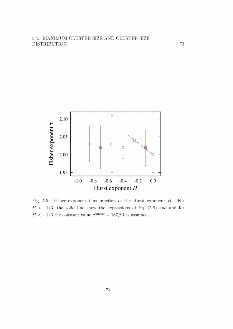
5.4. MAXIMUM CLUSTER SIZE AND CLUSTER SIZEDISTRIBUTION 73
1.95
2.00
2.05
2.10
-1.0 -0.8 -0.6 -0.4 -0.2 0.0
Fis
her
exponen
t τ
Hurst exponent H
Fig. 5.5: Fisher exponent t as function of the Hurst exponent H. For
H > −1/3, the solid line show the expressions of Eq. (5.9) and and for
H < −1/3 the constant value τuncorr = 187/91 is assumed.
73
74 CHAPTER 5. LONG-RANGE CORRELATED PERCOLATION
5.5 Cluster perimeters
Here, we consider triangular lattice stripes of aspect ratio A = 8. For
every largest cluster that spans the lattice vertically (between the long
sides of the lattice) and does not touch its vertical boundaries, there are
two contours that can be defined: the complete and accessible perime-
ters [5–7, 13–15, 62, 184–188]. Figure 5.6 shows the definition of the two
perimeters, which live on the dual of the original lattice, i.e. the honeycomb
lattice in the case of the triangular lattice. The complete perimeter consists
of all bonds of the honeycomb lattice that separate sites belonging to the
spanning cluster from unoccupied sites that can be reached from the verti-
cal boundaries of the lattice without crossing sites belonging to the largest
cluster. If, in addition, fjords of the perimeter with diameter less than√
3/3
(lattice units) are inaccessible, the accessible perimeter is obtained. Figure
5.7 shows the left hand side complete and accessible perimeters of a perco-
lating cluster on a lattice of size L = 128. In the upper inset of Fig. 5.8, the
length of the complete perimeter Mcp is observed to scale with the lattice
size L as,
Mcp ∼ Ldcp , (5.10)
where for the uncorrelated case, given by H = −1, it is known that dcp = 7/4
[5, 6, 62, 186]. In addition to considering the scaling of Mcp with L, we also
determined the fractal dimension dcp using the yardstick method [189, 190].
There, one measures the number of sticks S(m) of size m needed to follow the
perimeter from one end to the other. Figure 5.9 shows that, for intermediate
stick lengths, S(m) scales as
S ∼ m−dcp . (5.11)
We measured the value of the fractal dimension with this method for different
lattice sizes L, see Fig. 5.9, and then extrapolated the results to L→∞ to
obtain dcp. The fractal dimension dcp(H) determined by this method is com-
patible with the one obtained from the scaling of the length of the perimeter,
see Eq. (5.10), and we combined both measurements for the final estimates.
74
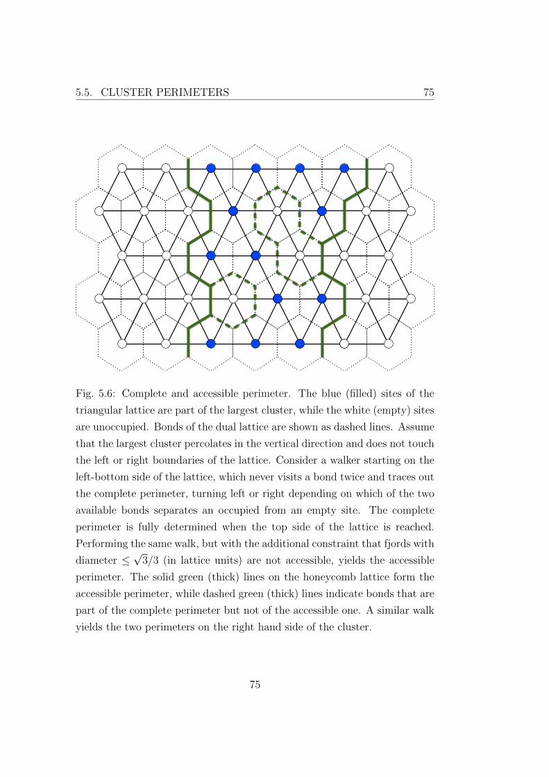
5.5. CLUSTER PERIMETERS 75
Fig. 5.6: Complete and accessible perimeter. The blue (filled) sites of the
triangular lattice are part of the largest cluster, while the white (empty) sites
are unoccupied. Bonds of the dual lattice are shown as dashed lines. Assume
that the largest cluster percolates in the vertical direction and does not touch
the left or right boundaries of the lattice. Consider a walker starting on the
left-bottom side of the lattice, which never visits a bond twice and traces out
the complete perimeter, turning left or right depending on which of the two
available bonds separates an occupied from an empty site. The complete
perimeter is fully determined when the top side of the lattice is reached.
Performing the same walk, but with the additional constraint that fjords with
diameter ≤√
3/3 (in lattice units) are not accessible, yields the accessible
perimeter. The solid green (thick) lines on the honeycomb lattice form the
accessible perimeter, while dashed green (thick) lines indicate bonds that are
part of the complete perimeter but not of the accessible one. A similar walk
yields the two perimeters on the right hand side of the cluster.
75

76 CHAPTER 5. LONG-RANGE CORRELATED PERCOLATION
(a) H = −1 (b) H = −0.5
(c) H = −0.25 (d) H = 0
Fig. 5.7: Snapshots of typical complete and accessible perimeters. The ac-
cessible perimeter is shown in bold solid blue lines. In addition, the parts
of the complete perimeter that do not belong to the accessible perimeter are
drawn with thin black lines. The snapshots are taken for (a) H = −1, (b)
−0.5, (c) −0.25, and (d) 0, on a lattice of (vertical) length L = 128.
76
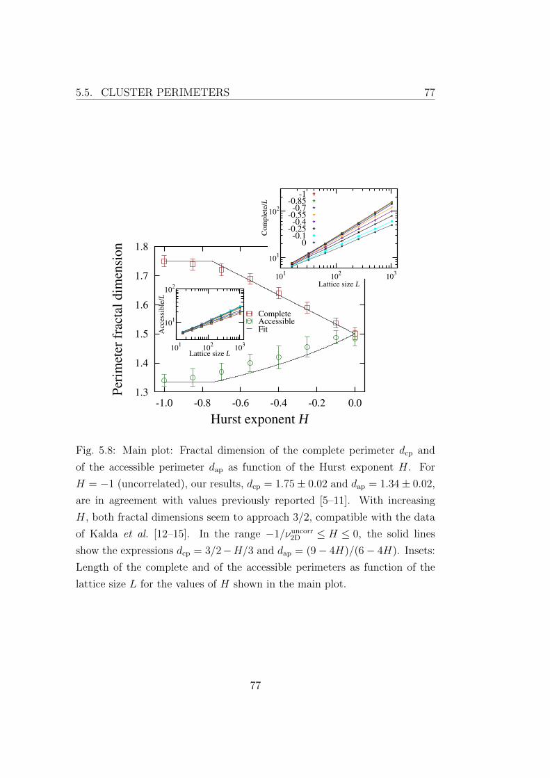
5.5. CLUSTER PERIMETERS 77
1.3
1.4
1.5
1.6
1.7
1.8
-1.0 -0.8 -0.6 -0.4 -0.2 0.0
Per
imet
er f
ract
al d
imen
sion
Hurst exponent H
CompleteAccessibleFit
101
102
101
102
103
Acc
essi
ble
/L
Lattice size L
101
102
101
102
103
Com
ple
te/L
Lattice size L
-1-0.85-0.7
-0.55-0.4
-0.25-0.1
0
Fig. 5.8: Main plot: Fractal dimension of the complete perimeter dcp and
of the accessible perimeter dap as function of the Hurst exponent H. For
H = −1 (uncorrelated), our results, dcp = 1.75± 0.02 and dap = 1.34± 0.02,
are in agreement with values previously reported [5–11]. With increasing
H, both fractal dimensions seem to approach 3/2, compatible with the data
of Kalda et al. [12–15]. In the range −1/νuncorr2D ≤ H ≤ 0, the solid lines
show the expressions dcp = 3/2−H/3 and dap = (9− 4H)/(6− 4H). Insets:
Length of the complete and of the accessible perimeters as function of the
lattice size L for the values of H shown in the main plot.
77
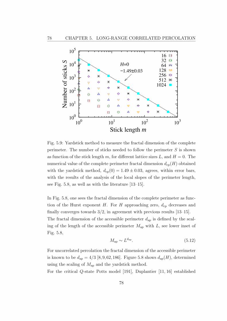
78 CHAPTER 5. LONG-RANGE CORRELATED PERCOLATION
100
101
102
103
104
105
100
101
102
103
Num
ber
of
stic
ks
S
Stick length m
H=0
−1.49±0.03
163264
128256512
1024
Fig. 5.9: Yardstick method to measure the fractal dimension of the complete
perimeter. The number of sticks needed to follow the perimeter S is shown
as function of the stick length m, for different lattice sizes L, and H = 0. The
numerical value of the complete perimeter fractal dimension dcp(H) obtained
with the yardstick method, dcp(0) = 1.49± 0.03, agrees, within error bars,
with the results of the analysis of the local slopes of the perimeter length,
see Fig. 5.8, as well as with the literature [13–15].
In Fig. 5.8, one sees the fractal dimension of the complete perimeter as func-
tion of the Hurst exponent H. For H approaching zero, dcp decreases and
finally converges towards 3/2, in agreement with previous results [13–15].
The fractal dimension of the accessible perimeter dap is defined by the scal-
ing of the length of the accessible perimeter Map with L, see lower inset of
Fig. 5.8,
Map ∼ Ldap . (5.12)
For uncorrelated percolation the fractal dimension of the accessible perimeter
is known to be dap = 4/3 [8,9,62,186]. Figure 5.8 shows dap(H), determined
using the scaling of Map and the yardstick method.
For the critical Q-state Potts model [191], Duplantier [11, 16] established
78
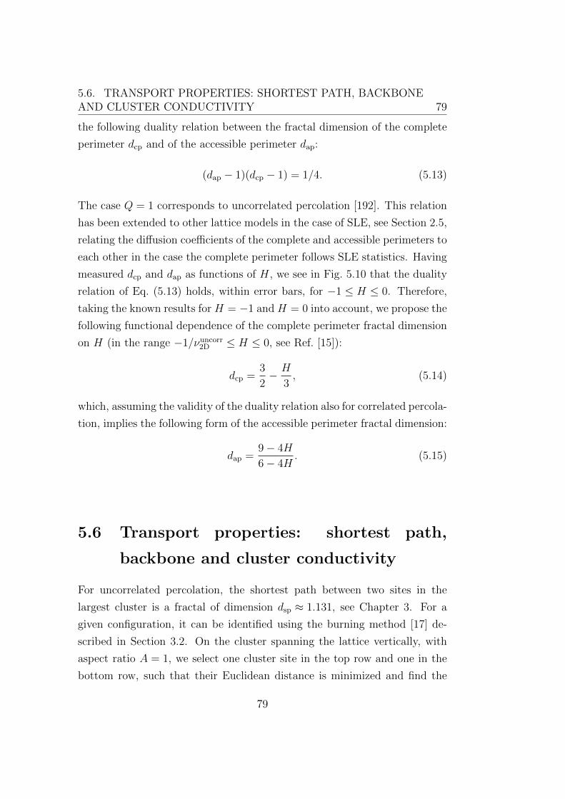
5.6. TRANSPORT PROPERTIES: SHORTEST PATH, BACKBONEAND CLUSTER CONDUCTIVITY 79
the following duality relation between the fractal dimension of the complete
perimeter dcp and of the accessible perimeter dap:
(dap − 1)(dcp − 1) = 1/4. (5.13)
The case Q = 1 corresponds to uncorrelated percolation [192]. This relation
has been extended to other lattice models in the case of SLE, see Section 2.5,
relating the diffusion coefficients of the complete and accessible perimeters to
each other in the case the complete perimeter follows SLE statistics. Having
measured dcp and dap as functions of H, we see in Fig. 5.10 that the duality
relation of Eq. (5.13) holds, within error bars, for −1 ≤ H ≤ 0. Therefore,
taking the known results for H = −1 and H = 0 into account, we propose the
following functional dependence of the complete perimeter fractal dimension
on H (in the range −1/νuncorr2D ≤ H ≤ 0, see Ref. [15]):
dcp =3
2− H
3, (5.14)
which, assuming the validity of the duality relation also for correlated percola-
tion, implies the following form of the accessible perimeter fractal dimension:
dap =9− 4H
6− 4H. (5.15)
5.6 Transport properties: shortest path,
backbone and cluster conductivity
For uncorrelated percolation, the shortest path between two sites in the
largest cluster is a fractal of dimension dsp ≈ 1.131, see Chapter 3. For a
given configuration, it can be identified using the burning method [17] de-
scribed in Section 3.2. On the cluster spanning the lattice vertically, with
aspect ratio A = 1, we select one cluster site in the top row and one in the
bottom row, such that their Euclidean distance is minimized and find the
79
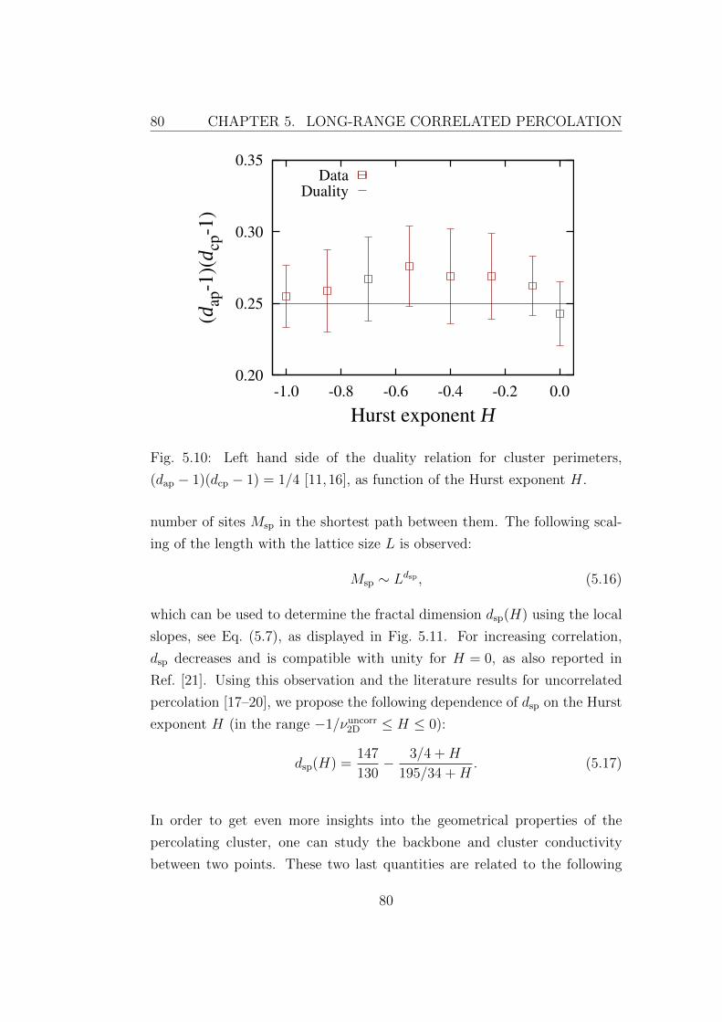
80 CHAPTER 5. LONG-RANGE CORRELATED PERCOLATION
0.20
0.25
0.30
0.35
-1.0 -0.8 -0.6 -0.4 -0.2 0.0
(dap
-1)(
d cp-1
)
Hurst exponent H
DataDuality
Fig. 5.10: Left hand side of the duality relation for cluster perimeters,
(dap − 1)(dcp − 1) = 1/4 [11,16], as function of the Hurst exponent H.
number of sites Msp in the shortest path between them. The following scal-
ing of the length with the lattice size L is observed:
Msp ∼ Ldsp , (5.16)
which can be used to determine the fractal dimension dsp(H) using the local
slopes, see Eq. (5.7), as displayed in Fig. 5.11. For increasing correlation,
dsp decreases and is compatible with unity for H = 0, as also reported in
Ref. [21]. Using this observation and the literature results for uncorrelated
percolation [17–20], we propose the following dependence of dsp on the Hurst
exponent H (in the range −1/νuncorr2D ≤ H ≤ 0):
dsp(H) =147
130− 3/4 +H
195/34 +H. (5.17)
In order to get even more insights into the geometrical properties of the
percolating cluster, one can study the backbone and cluster conductivity
between two points. These two last quantities are related to the following
80
5.6. TRANSPORT PROPERTIES: SHORTEST PATH, BACKBONEAND CLUSTER CONDUCTIVITY 81
0.95
1.00
1.05
1.10
1.15
1.20
1.25
-1.0 -0.8 -0.6 -0.4 -0.2 0.0
Short
est
pat
h d
sp
Hurst exponent H
DataFit
101
102
103
104
101
102
103
Pat
h l
ength
Lattice size L
-1-0.85-0.7
-0.55-0.4
-0.25-0.1
0
Fig. 5.11: Fractal dimension of the shortest path dsp of the largest clus-
ter as function of the Hurst exponent H. The inset shows the number
of sites in the shortest path as function of the lattice size L for the same
value of H as in the main plot. For uncorrelated disorder, i.e. H = −1,
we find dsp = 1.130± 0.005, in agreement with the literature [17–20]. With
increasing Hurst exponent, dsp approaches unity [21]. The solid line is
the graph of the proposed behavior of the shortest path fractal dimen-
sion: dsp(H) = 147/130− (3/4 +H)/(195/34 +H), for −3/4 ≤ H ≤ 0, and
dsp(−1 ≤ H ≤ −1/νuncorr2D ) = dsp(−1/νuncorr
2D ) = 147/130.
81
82 CHAPTER 5. LONG-RANGE CORRELATED PERCOLATION
question. If one supposes that the occupied sites of the percolating cluster
are resistors and a potential difference is applied between these two sites,
which sites would carry non-zero current? This subset of sites of the largest
cluster is called effective backbone [193] and is related to the geometrical
backbone defined as the union of all non-self-crossing paths between these
two sites [17,19,23–26,65,82]. Actually some sites, called perfectly balanced
sites [193], belong to the geometrical backbone but do not carry current,
because the potentials are perfectly balanced, and therefore do not belong to
the effective backbone. Algorithmically, for a given cluster, the geometrical
backbone can be found with the burning method described in Ref. [17]. It
works as follows. One first burns the sites of the spanning cluster starting
from the lower site and indexes the burned sites according to the time they
have been reached, till the higher edge is reached. Then one does a second
burning, starting from the higher edge, but only burning sites with a lower
index as defined in the first burning. This identifies the so-called elastic
backbone, which is the union of all the shortest paths between the two points.
One then grows the backbone as follows, starting from the elastic backbone.
One starts a third burning. For each site where a loop was closed in the
first burning, one burns the sites with a lower index, with the condition that
the growning backbone cannot burn. One reaches the growning backbone
whether at a single point or at several points. Only in the case where the
growing backbone is reached at several points, all the points that have been
burned are added to the growing backbone. One repeats this procedure, till
no more part can be attached to the growing backbone and one obtains the
full backbone.
Other methods based on the conductivity properties rather than the geo-
metrical properties of the backbone have been developed [193, 194]. They
actually compute the current passing through every node of the largest clus-
ter. The advantage of using the geometrical properties of the backbone over
methods solving Kirchoff’s law to determine which bonds carry current or
not is that the burning algorithm presented above is fast (there is no matrix
to invert, see later) and computes exactly the geometrical backbone, whereas
the other methods computes only the effective backbone. In the following
82
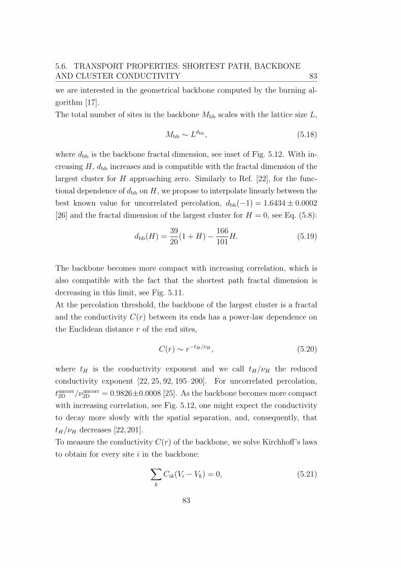
5.6. TRANSPORT PROPERTIES: SHORTEST PATH, BACKBONEAND CLUSTER CONDUCTIVITY 83
we are interested in the geometrical backbone computed by the burning al-
gorithm [17].
The total number of sites in the backbone Mbb scales with the lattice size L,
Mbb ∼ Ldbb , (5.18)
where dbb is the backbone fractal dimension, see inset of Fig. 5.12. With in-
creasing H, dbb increases and is compatible with the fractal dimension of the
largest cluster for H approaching zero. Similarly to Ref. [22], for the func-
tional dependence of dbb on H, we propose to interpolate linearly between the
best known value for uncorrelated percolation, dbb(−1) = 1.6434± 0.0002
[26] and the fractal dimension of the largest cluster for H = 0, see Eq. (5.8):
dbb(H) =39
20(1 +H)− 166
101H. (5.19)
The backbone becomes more compact with increasing correlation, which is
also compatible with the fact that the shortest path fractal dimension is
decreasing in this limit, see Fig. 5.11.
At the percolation threshold, the backbone of the largest cluster is a fractal
and the conductivity C(r) between its ends has a power-law dependence on
the Euclidean distance r of the end sites,
C(r) ∼ r−tH/νH , (5.20)
where tH is the conductivity exponent and we call tH/νH the reduced
conductivity exponent [22, 25, 92, 195–200]. For uncorrelated percolation,
tuncorr2D /νuncorr
2D = 0.9826±0.0008 [25]. As the backbone becomes more compact
with increasing correlation, see Fig. 5.12, one might expect the conductivity
to decay more slowly with the spatial separation, and, consequently, that
tH/νH decreases [22,201].
To measure the conductivity C(r) of the backbone, we solve Kirchhoff’s laws
to obtain for every site i in the backbone:∑k
Cik(Vi − Vk) = 0, (5.21)
83
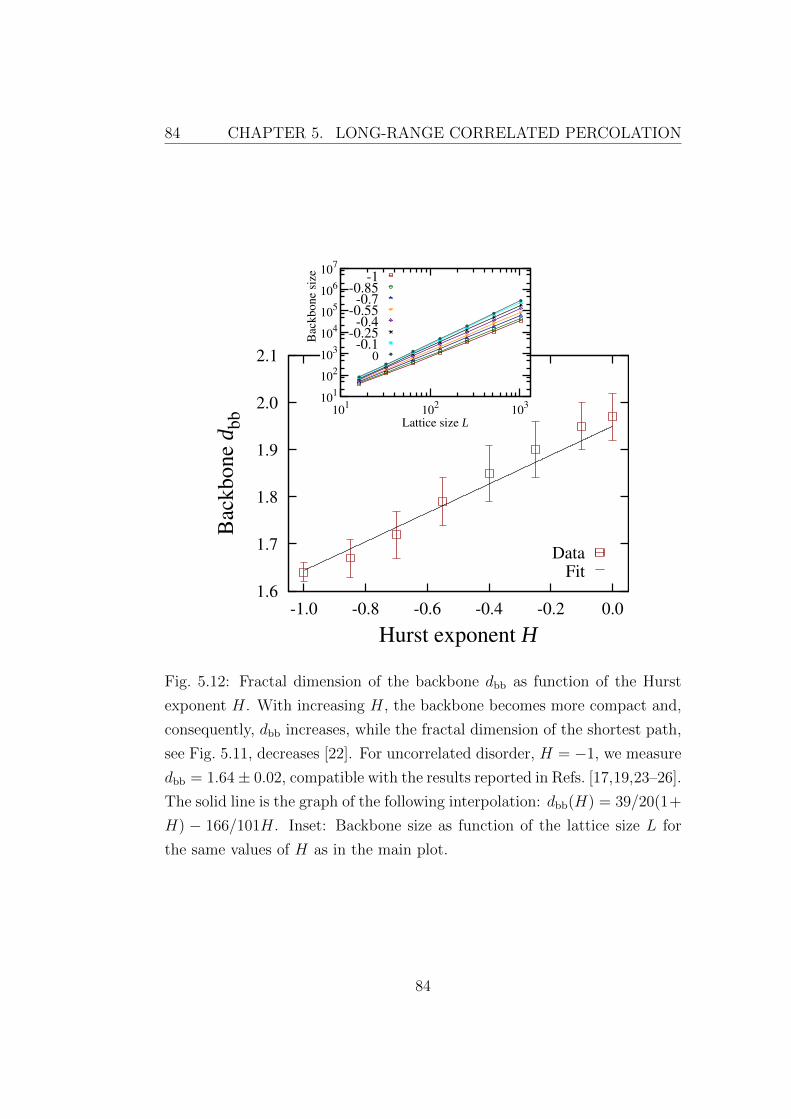
84 CHAPTER 5. LONG-RANGE CORRELATED PERCOLATION
1.6
1.7
1.8
1.9
2.0
2.1
-1.0 -0.8 -0.6 -0.4 -0.2 0.0
Bac
kbone
d bb
Hurst exponent H
DataFit
101
102
103
104
105
106
107
101
102
103
Bac
kb
on
e si
ze
Lattice size L
-1-0.85
-0.7-0.55
-0.4-0.25
-0.10
Fig. 5.12: Fractal dimension of the backbone dbb as function of the Hurst
exponent H. With increasing H, the backbone becomes more compact and,
consequently, dbb increases, while the fractal dimension of the shortest path,
see Fig. 5.11, decreases [22]. For uncorrelated disorder, H = −1, we measure
dbb = 1.64± 0.02, compatible with the results reported in Refs. [17,19,23–26].
The solid line is the graph of the following interpolation: dbb(H) = 39/20(1+
H) − 166/101H. Inset: Backbone size as function of the lattice size L for
the same values of H as in the main plot.
84
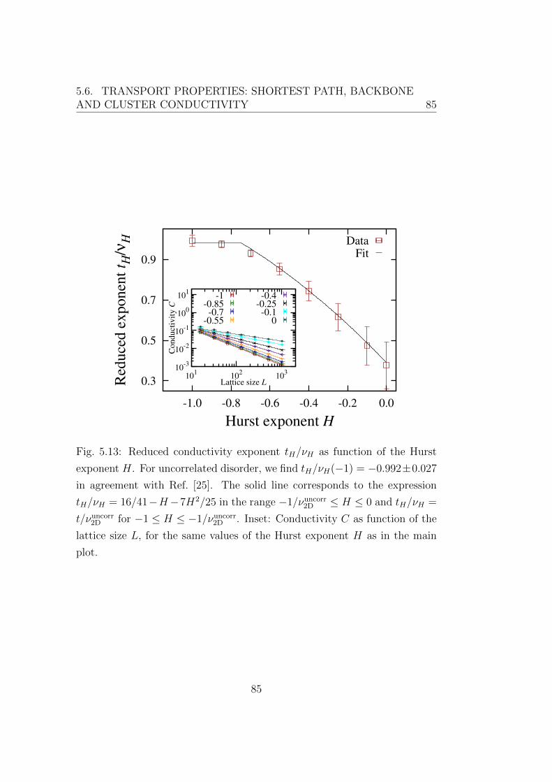
5.6. TRANSPORT PROPERTIES: SHORTEST PATH, BACKBONEAND CLUSTER CONDUCTIVITY 85
0.3
0.5
0.7
0.9
-1.0 -0.8 -0.6 -0.4 -0.2 0.0
Red
uce
d e
xponen
t t H
/νH
Hurst exponent H
DataFit
10-3
10-2
10-1
100
101
101
102
103
Co
nd
uct
ivit
y C
Lattice size L
-1-0.85
-0.7-0.55
-0.4-0.25
-0.10
Fig. 5.13: Reduced conductivity exponent tH/νH as function of the Hurst
exponent H. For uncorrelated disorder, we find tH/νH(−1) = −0.992±0.027
in agreement with Ref. [25]. The solid line corresponds to the expression
tH/νH = 16/41−H−7H2/25 in the range −1/νuncorr2D ≤ H ≤ 0 and tH/νH =
t/νuncorr2D for −1 ≤ H ≤ −1/νuncorr
2D . Inset: Conductivity C as function of the
lattice size L, for the same values of the Hurst exponent H as in the main
plot.
85
86 CHAPTER 5. LONG-RANGE CORRELATED PERCOLATION
where the sum runs over the nearest neighbors k and the conductivity Cik
is unity if the site k also belongs to the backbone and zero otherwise. The
boundary conditions are chosen such that Vtop = N on the top end of the
backbone and Vbottom = 0 on its bottom end. In order to solve this linear
system of equations, we invert the sparse conductivity matrix C of elements
Cik, using a sparse matrix solver1 and obtain the value of the potential Vi at
each site i of the backbone2. From this we deduce the global conductivity as
follows [92]. As one knows the potentials at each site and the resistors are set
to unity, one is able to compute the currents in the system and especially the
total current Itot entering the top end of the backbone. From this one deduce
the global conductivity Ctot through the relation Ctot = Itot/(Vtop− Vbottom).
The inset of Fig. 5.13 shows the conductivity C as function of the lattice
size L, for different values of H. Since in our setup the distance between the
end points r ∼ L, we use this scaling to determine the reduced conductivity
exponent tH/νH , see Fig. 5.13. Our result for uncorrelated percolation agrees
with the literature and one observes that tH/νH decreases with increasing H.
We propose the following functional dependence of the reduced conductivity
exponent on H (in the range −1/νuncorr2D ≤ H ≤ 0):
tHνH
=16
41−H − 7H2
25. (5.22)
5.7 Final remarks
Concluding, we studied percolation with long-range correlation in the site
occupation probabilities, as characterized by the Hurst exponent H. The
site percolation threshold of the triangular lattice was argued to be 1/2,
independent of H. For H approaching zero the fractal dimension of the
largest cluster was found to increase, meaning that the largest cluster gets
more dense for increasing values of H. Also the cluster size distribution was
1To invert the sparse matrix C we use the Intel MKL Direct Sparse Solver.2Solving Kirchoff’s law only for the backbone and not for the full largest cluster, as
done in Ref. [194], is computationally more effective as the conductivity matrix C to be
inverted is much smaller.
86
5.7. FINAL REMARKS 87
shown to follow a power law dependence with its critical exponent decreasing
towards 2 for H going to zero. The fractal dimensions of the complete and
accessible perimeters of the largest cluster were observed to approach 3/2 for
H → 0, while the duality relation between both fractal dimensions seems to
hold independently of the value of H. As H increased, the fractal dimension
of the shortest path was observed to decrease towards 1 for H going to 0. This
is in agreement with the backbone becoming more compact with increasing
value of H, as does the largest cluster. This has also an influence on the
cluster conductivity, such that the reduced conductivity exponent decreases
with H. We also proposed quantitative relations for the dependence of the
studied critical exponents of the percolation transition on H, as being the
simplest rational expressions that fit the numerical data.
87

88 CHAPTER 5. LONG-RANGE CORRELATED PERCOLATION
88
Chapter 6
Schramm-Loewner Evolution
on long-range correlated
landscapes
In the previous Chapter we have seen how the power-law correlations modify
the geometrical properties of the largest cluster, and conjectured quantitative
relations for the dependency of the critical exponents on the Hurst exponent
H ∈ [−1, 0]. In this Chapter, we go beyond the description in terms of crit-
ical exponents and study the paths at criticality in the framework of SLE.
We analyze the statistical properties of the zero isoheight lines for corre-
lated landscapes for H ∈ [−1, 1]. We show numerically that for H ≤ 0 the
statistics of these lines is compatible with SLEκ for κ ∈ [8/3, 4], and that
established analytical results are recovered for H = −1 and H = 0. This
result suggests that for negative Hurst exponent in spite of the long-range na-
ture of correlations, surprisingly the statistics of isolines is fully encoded in a
Markovian Brownian motion with a single parameter in the continuum limit.
However, for strictly positive Hurst exponent, we find that the underlying
driving function is not Markovian and therefore not consistent with SLEκ.
We also analyze the shortest path at criticality and the watersheds, but, in
contrast to the the case of the isoheight lines, we do not find agreement with
SLE statistics in the case of correlated landscapes, i.e. for H > −1.
89
90CHAPTER 6. SCHRAMM-LOEWNER EVOLUTION ON
LONG-RANGE CORRELATED LANDSCAPES
This Chapter is based on:
N. Pose, K. J. Schrenk, N. A. M. Araujo, and H. J. Herrmann, Schramm-
Loewner Evolution on correlated landscapes, in progress.
6.1 Introduction
In this Chapter we map isoheight lines of long-range correlated landscapes on
uncorrelated random walks. These lines are extracted from the landscapes
by following paths at a given height [55]. In the case of land scenes, the lines
correspond to the boundary of lakes or seas [55] but one can also consider
energy landscapes where isoheight lines are paths of constant energy [120,
130], or vorticity fields in turbulence where these lines correspond to the
vortex lines [32]. These isoheight lines are usually scale invariant [12, 189]
and empirical results on rocky shorelines suggest that isoheight lines are even
conformally invariant [55]. The long-range correlations of the landscapes
are parametrized by their Hurst exponent H ∈ [−1, 1] and we show that
in the case H ≤ 0 the statistical properties of the zero isoheight lines are
compatible with SLE [29]. This allows to map the long-range correlated lines
of landscapes characterized by their Hurst exponent onto one-dimensional
Markovian processes.
This is done by finding the conformal maps gt that iteratively map the com-
plement of the curve in the upper half-plane H back onto H and satisfies
Loewner’s differential equation Eq. (2.10),
∂gt(z)
∂t=
2
gt(z)− ξt,
with g0(z) = z and ξt a real continuous function. In the case of SLEκ the
driving function ξt is equal to ξt =√κBt with Bt a standard one-dimensional
Brownian motion, and κ a diffusion constant. Therefore studying the iso-
height lines for H ∈ [−1, 0] and relating them to the SLE theory, shows
that the statistics of the isoheight lines is encoded in a Markovian process,
consisting of a Brownian motion of diffusivity κ. As the fractal dimension
of the isoheight lines depends on the value of the Hurst exponent H, see
90
6.2. ISOHEIGHT LINES ON CORRELATED LANDSCAPES WITHNEGATIVE HURST EXPONENT 91
Section 5.5, and the fractal dimension of SLEκ curves depends on the value
of κ, see Section 2.7.1, one expects a relation between the value of κ and H
for the isoheight lines. Below we focus on the accessible perimeter of zero
isoheight lines on triangular lattices of size Lx × Ly with Lx = 8Ly [99].
6.2 Isoheight lines on correlated landscapes
with negative Hurst exponent
We consider random landscapes on a lattice. To each site x = (x, y) on the
lattice one associates a random height h(x). We suppose that the heights
have long-range correlations of the form:
c(r) = 〈h(x)h(x + r)〉x ∼ |r|2H , (6.1)
where H is the Hurst exponent. Using the Wiener-Khintchine theorem [132]
relating the height-height correlation function c(r) to the power spectrum,
one generates random landscapes on a finite lattice using the Fourier filtering
method, see Section 4.3. As mentionned in Chapter 4, one recovers uncor-
related landscapes for H = −1, and the discrete Gaussian Free Field (GFF)
for H = 0 [39]. To identify the complete perimeter of the isoheight lines
one extracts the interface on the dual lattice between the sites lower and the
sites higher than a given height hc. One can map these isoheight lines to the
perimeters of percolation clusters, like in Fig. 4.1 , where the sites above hc
are marked as occupied and the sites below hc as empty. One can then define
the accessible perimeter as the complete perimeter from which one suppresses
the fjords of neck size equal to the lattice unit of the dual lattice, i.e.√
3/3,
see Fig. 5.6. It has been shown in Section 5.3, that on the triangular lattice
a spanning cluster emerges at a critical height hc = 0. Therefore we consider
the percolating clusters at hc = 0 and extract their complete and accessible
perimeters that span from the bottom line to the top line. In order to study
the SLE properties of these isoheight lines using the chordal SLE formalism,
we map them into the upper half-plane using the methodology described in
Section 2.6.
91

92CHAPTER 6. SCHRAMM-LOEWNER EVOLUTION ON
LONG-RANGE CORRELATED LANDSCAPES
The zero isoheight lines on the triangular lattice in the case of percolation
and of the GFF are analytically tractable and it has been proven that they
are SLE [29,35,61].
6.2.1 SLE and fractal dimension
As proven by Beffara [52], SLEκ curves are fractals of a fractal dimension df
that is related to the diffusion coefficient κ as:
df = min(
2, 1 +κ
8
).
The fractal dimension df of the accessible perimeter of the isoheight lines
for different values of H was numerically estimated and even a conjecture
was proposed for its dependence on H in Section 5.5. Using the equation
above, one gets a first estimate of the expected values of κ for SLE curves
of the same fractal dimension, see Table 6.2. For H = −1 and H = 0, the
values of the fractal dimension and diffusivity are known exactly: df = 4/3,
κ = 8/3, and df = 3/2, κ = 4, respectively. We will compare this result to
the estimates of κ obtained with two indirect methods, the winding angle
and the left passage probability, and with the one obtained from the direct
SLE method.
6.2.2 Winding angle
The winding angle of SLEκ curves follows a Gaussian distribution and the
variance scales with κ as,
〈θ2〉 − 〈θ〉2 = σ2θ = b+
κ
4ln(Ly),
where b is a constant and Ly is the vertical lattice size [29, 53, 54]. κ/4
corresponds to the slope of σ2θ vs ln(Ly). The estimates of κ are displayed in
Table 6.2.
For values near H = 0, one has less precision on the results, as the system
is strongly influenced by finite-size effects, see Fig. 5.1 in Chapter 4. The
result we obtain from the winding angle measurement is, within error bars,
92

6.2. ISOHEIGHT LINES ON CORRELATED LANDSCAPES WITHNEGATIVE HURST EXPONENT 93
Ly
101 102 103
4(<
2 3!
b)=5
2
3
4
5
6
70-0.1-0.25-0.4-0.55-0.7-0.85-1
3=<3-5 0 5
<!
13
P(3
)
0
0.2
0.4
Fig. 6.1: Rescaled variance of the winding angle along the curve for different
Hurst exponents H = −1,−0.85,−0.7,−0.55,−0.4,−0.25,−0.1, 0. The rela-
tionσ2θ−bκ/4
= lnLy is displayed by the black solid line. In the inset, the rescaled
probability distributions are plotted and compared to a normal distribution
for H = −1,−0.55, 0.
93
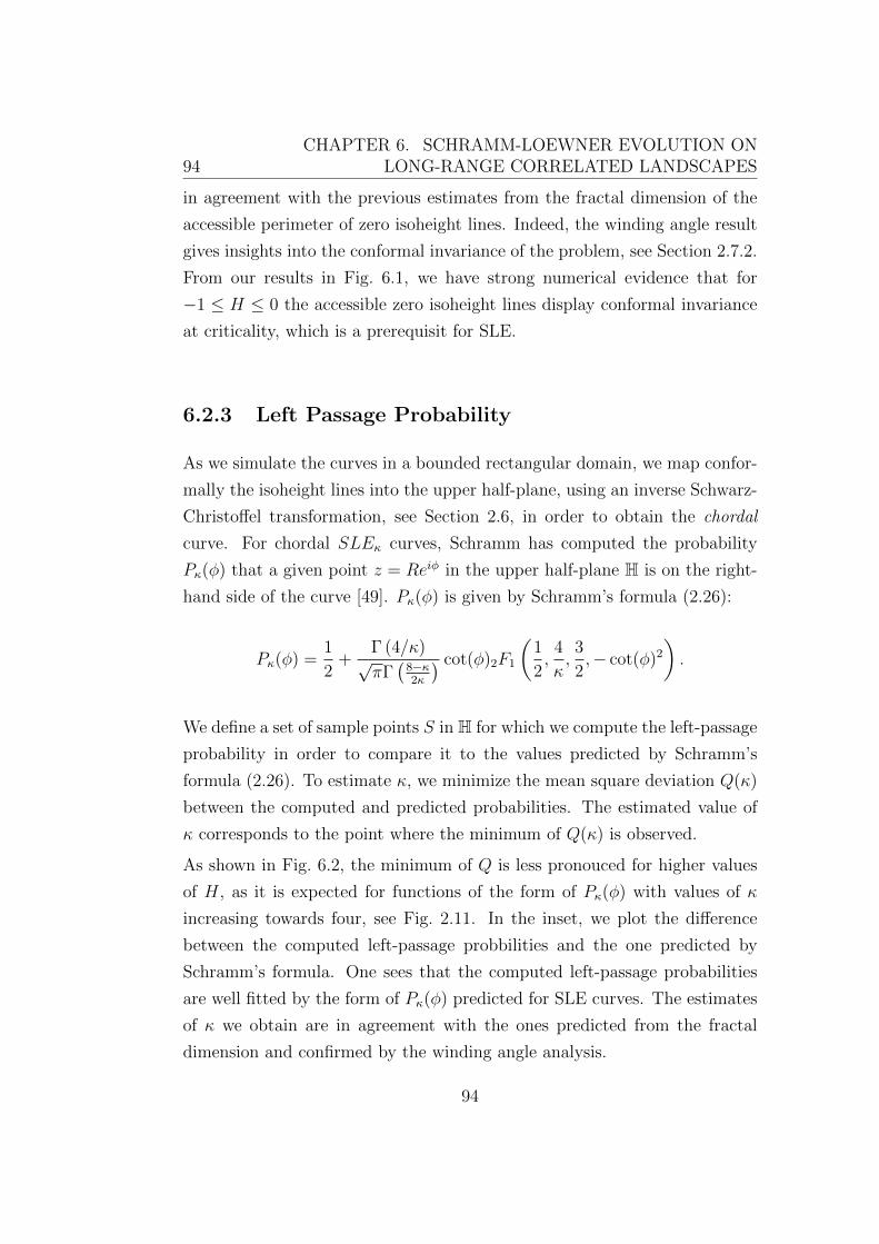
94CHAPTER 6. SCHRAMM-LOEWNER EVOLUTION ON
LONG-RANGE CORRELATED LANDSCAPES
in agreement with the previous estimates from the fractal dimension of the
accessible perimeter of zero isoheight lines. Indeed, the winding angle result
gives insights into the conformal invariance of the problem, see Section 2.7.2.
From our results in Fig. 6.1, we have strong numerical evidence that for
−1 ≤ H ≤ 0 the accessible zero isoheight lines display conformal invariance
at criticality, which is a prerequisit for SLE.
6.2.3 Left Passage Probability
As we simulate the curves in a bounded rectangular domain, we map confor-
mally the isoheight lines into the upper half-plane, using an inverse Schwarz-
Christoffel transformation, see Section 2.6, in order to obtain the chordal
curve. For chordal SLEκ curves, Schramm has computed the probability
Pκ(φ) that a given point z = Reiφ in the upper half-plane H is on the right-
hand side of the curve [49]. Pκ(φ) is given by Schramm’s formula (2.26):
Pκ(φ) =1
2+
Γ (4/κ)√πΓ(
8−κ2κ
) cot(φ)2F1
(1
2,
4
κ,3
2,− cot(φ)2
).
We define a set of sample points S in H for which we compute the left-passage
probability in order to compare it to the values predicted by Schramm’s
formula (2.26). To estimate κ, we minimize the mean square deviation Q(κ)
between the computed and predicted probabilities. The estimated value of
κ corresponds to the point where the minimum of Q(κ) is observed.
As shown in Fig. 6.2, the minimum of Q is less pronouced for higher values
of H, as it is expected for functions of the form of Pκ(φ) with values of κ
increasing towards four, see Fig. 2.11. In the inset, we plot the difference
between the computed left-passage probbilities and the one predicted by
Schramm’s formula. One sees that the computed left-passage probabilities
are well fitted by the form of Pκ(φ) predicted for SLE curves. The estimates
of κ we obtain are in agreement with the ones predicted from the fractal
dimension and confirmed by the winding angle analysis.
94

6.2. ISOHEIGHT LINES ON CORRELATED LANDSCAPES WITHNEGATIVE HURST EXPONENT 95
5=5min
0.9 0.95 1 1.05 1.1
Q(5
)=Q
(5m
in)
1
2
3
4
5
60-0.1-0.25-0.4-0.55-0.7-0.85-1
3=:0 0.5 1
P(3
)!
P5(3
)
-0.1
0
0.1
Fig. 6.2: Measured rescaled mean square deviation Q(κ)/Q(κmin) as
a function of κ/κmin with κmin the value of κ where the min-
imum of Q(κ) is attained, for different Hurst exponents H =
−1,−0.85,−0.7,−0.55,−0.4,−0.25,−0.1, 0. In the inset, the difference be-
tween the measured left passage probabilities P (θ) and the left passage prob-
abilities Pκ(θ) predicted by Schramm’s formula of Eq. (2.26) with κ = κmin,
for H = −0.85,−0.55,−0.25, 0. For convenience, we chose 502 points in the
range [−0.025Lx, 0.025Lx]× [0.15Ly, 0.25Ly] with Ly = 1024 and Lx = 8Ly,
which are then mapped to the upper half-plane through an inverse Schwarz-
Christoffel transformation, see Section 2.6.
95
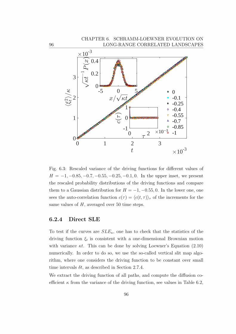
96CHAPTER 6. SCHRAMM-LOEWNER EVOLUTION ON
LONG-RANGE CORRELATED LANDSCAPES
t #10-30 1 2 3
h92 ti=5
#10-3
0
1
2
3
0-0.1-0.25-0.4-0.55-0.7-0.85-1
x=p5t
-5 0 5
p5t!
1P
(x)
0
0.2
0.4
=0 2
c(=)
-1
0
1
#10!3
Fig. 6.3: Rescaled variance of the driving functions for different values of
H = −1,−0.85,−0.7,−0.55,−0.25,−0.1, 0. In the upper inset, we present
the rescaled probability distributions of the driving functions and compare
them to a Gaussian distribution for H = −1,−0.55, 0. In the lower one, one
sees the auto-correlation function c(τ) = 〈c(t, τ)〉τ of the increments for the
same values of H, averaged over 50 time steps.
6.2.4 Direct SLE
To test if the curves are SLEκ, one has to check that the statistics of the
driving function ξt is consistent with a one-dimensional Brownian motion
with variance κt. This can be done by solving Loewner’s Equation (2.10)
numerically. In order to do so, we use the so-called vertical slit map algo-
rithm, where one considers the driving function to be constant over small
time intervals δt, as described in Section 2.7.4.
We extract the driving function of all paths, and compute the diffusion co-
efficient κ from the variance of the driving function, see values in Table 6.2,
96
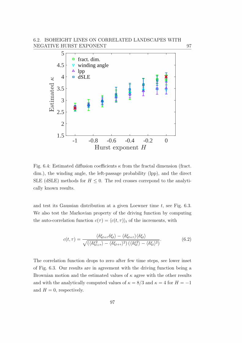
6.2. ISOHEIGHT LINES ON CORRELATED LANDSCAPES WITHNEGATIVE HURST EXPONENT 97
Hurst exponent H-1 -0.8 -0.6 -0.4 -0.2 0
Est
imate
d5
1.5
2
2.5
3
3.5
4
4.5
5fract. dim.winding anglelppdSLE
Fig. 6.4: Estimated diffusion coefficients κ from the fractal dimension (fract.
dim.), the winding angle, the left-passage probability (lpp), and the direct
SLE (dSLE) methods for H ≤ 0. The red crosses correpond to the analyti-
cally known results.
and test its Gaussian distribution at a given Loewner time t, see Fig. 6.3.
We also test the Markovian property of the driving function by computing
the auto-correlation function c(τ) = 〈c(t, τ)〉t of the increments, with
c(t, τ) =〈δξt+τδξt〉 − 〈δξt+τ 〉〈δξt〉√
(〈δξ2t+τ 〉 − 〈δξt+τ 〉2) (〈δξ2
t 〉 − 〈δξt〉2). (6.2)
The correlation function drops to zero after few time steps, see lower inset
of Fig. 6.3. Our results are in agreement with the driving function being a
Brownian motion and the estimated values of κ agree with the other results
and with the analytically computed values of κ = 8/3 and κ = 4 for H = −1
and H = 0, respectively.
97
98CHAPTER 6. SCHRAMM-LOEWNER EVOLUTION ON
LONG-RANGE CORRELATED LANDSCAPES
6.3 Isoheight lines on correlated landscapes
with positive Hurst exponent
We apply the same tests for Gaussian random landscapes with positive Hurst
exponent H > 0, but contrary to the case H < 0 we do not find agreement
with SLEκ.
6.3.1 Winding angle
We apply the winding angle test to the zero isoheight lines of landscapes
with positive H to estimate κ, and find that the estimate of κ deduced from
the winding angle measurement strongly depends on the value of H ≥ 0. We
get an agreement between the estimates of κ from the fractal dimension of
the curves and of the winding angle measurement, see Fig. 6.5. However for
increasing values of H, one sees a slower convergence towards a linear behavior
of the variance, and a larger difference of the probability distribution from a
Gaussian distribution. This could be due to finite size effects.
6.3.2 Left-Passage probability
We now apply the left-passage probability test to the isoheights in the case
of positive Hurst exponent. The estimates of κ are displayed in Fig. 6.6,
where we plot the reduced mean square deviation Q(κ)/Q(κmin) as a function
of κ. One sees that contrary to what one expects from the winding angle
measurement, we do not find a strong dependence of the estimate of κ on the
value of H. In particular, this is in contradiction with the strong dependence
of the value of the fractal dimension of the isoheight lines on the value of H.
6.3.3 Direct SLE method
We extract the driving function from the isoheight lines and compute the
variance, the probability distribution and the autocorrelation function of the
increments. From the variance of the driving function, see Fig. 6.7, one ob-
tains that the estimate of κ depends strongly on H, but that it is not in
98
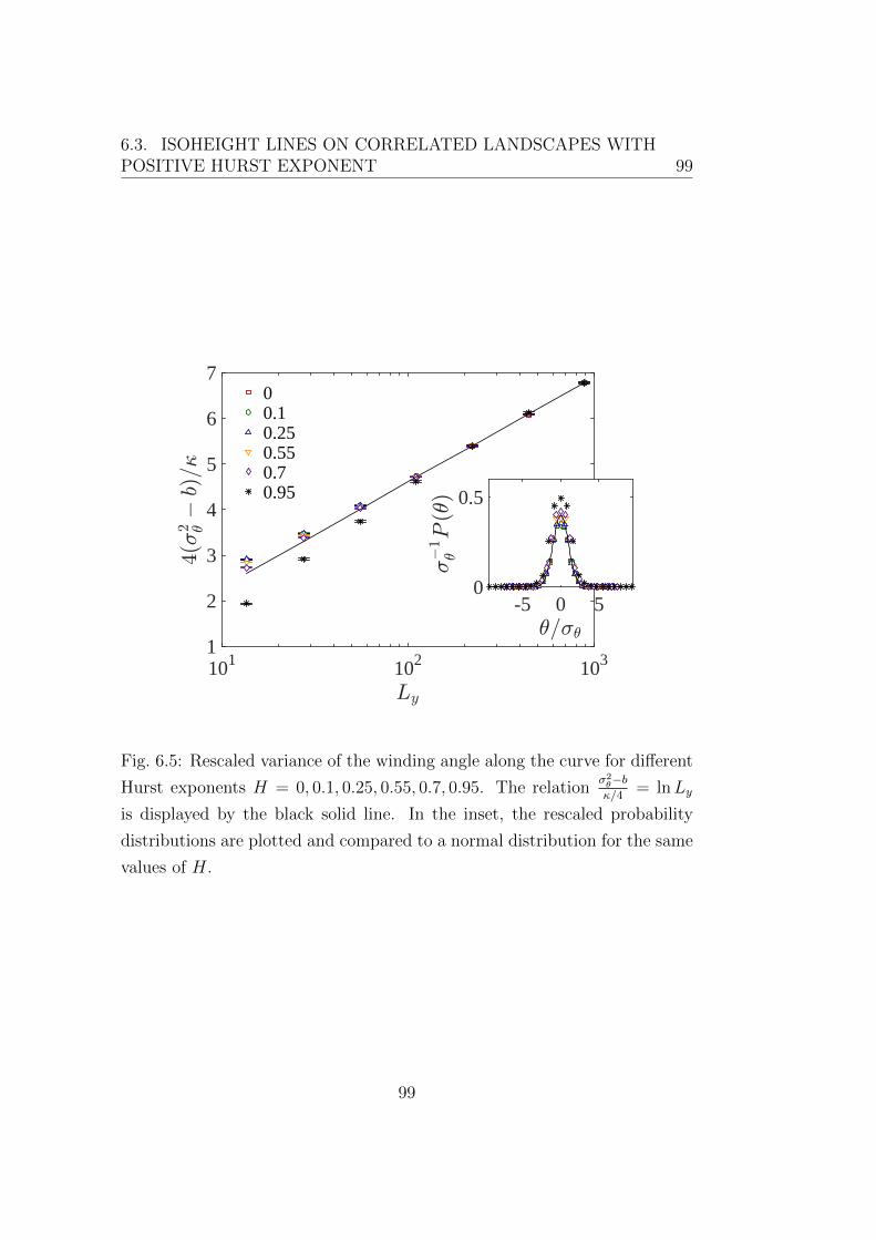
6.3. ISOHEIGHT LINES ON CORRELATED LANDSCAPES WITHPOSITIVE HURST EXPONENT 99
Ly
101 102 103
4(<
2 3!
b)=5
1
2
3
4
5
6
700.10.250.550.70.95
3=<3-5 0 5
<!
13
P(3
)
0
0.5
Fig. 6.5: Rescaled variance of the winding angle along the curve for different
Hurst exponents H = 0, 0.1, 0.25, 0.55, 0.7, 0.95. The relationσ2θ−bκ/4
= lnLy
is displayed by the black solid line. In the inset, the rescaled probability
distributions are plotted and compared to a normal distribution for the same
values of H.
99

100CHAPTER 6. SCHRAMM-LOEWNER EVOLUTION ON
LONG-RANGE CORRELATED LANDSCAPES
53 3.2 3.4 3.6 3.8 4
Q(5
)=Q
(5m
in)
1
1.2
1.4
1.6
1.8
2 00.10.250.550.70.95
Fig. 6.6: Measured rescaled mean square deviation Q(κ)/Q(κmin) as a func-
tion of κ, with κmin the value of κ where the minimum of Q(κ) is attained, for
different Hurst exponents H = 0, 0.1, 0.25, 0.55, 0.7, 0.95. For convenience,
we chose 502 points in the range [−0.025Lx, 0.025Lx]× [0.15Ly, 0.25Ly] with
Ly = 1024 and Lx = 8Ly, which are then mapped to the upper half-plane
through an inverse Schwarz-Christoffel transformation, see Section 2.6.
100
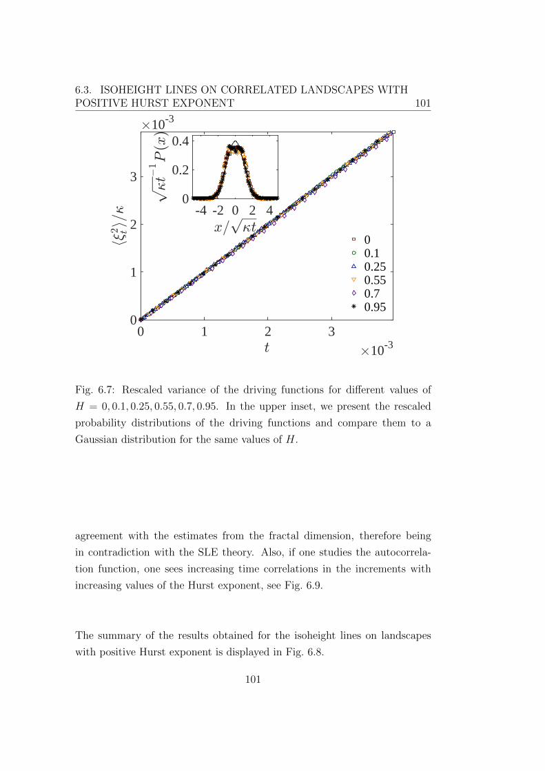
6.3. ISOHEIGHT LINES ON CORRELATED LANDSCAPES WITHPOSITIVE HURST EXPONENT 101
t #10-30 1 2 3
h92 ti=5
#10-3
0
1
2
3
00.10.250.550.70.95
x=p5t
-4 -2 0 2 4
p5t!
1P
(x)
0
0.2
0.4
Fig. 6.7: Rescaled variance of the driving functions for different values of
H = 0, 0.1, 0.25, 0.55, 0.7, 0.95. In the upper inset, we present the rescaled
probability distributions of the driving functions and compare them to a
Gaussian distribution for the same values of H.
agreement with the estimates from the fractal dimension, therefore being
in contradiction with the SLE theory. Also, if one studies the autocorrela-
tion function, one sees increasing time correlations in the increments with
increasing values of the Hurst exponent, see Fig. 6.9.
The summary of the results obtained for the isoheight lines on landscapes
with positive Hurst exponent is displayed in Fig. 6.8.
101

102CHAPTER 6. SCHRAMM-LOEWNER EVOLUTION ON
LONG-RANGE CORRELATED LANDSCAPES
Hurst exponent H0 0.2 0.4 0.6 0.8 1
Est
imate
d5
0
2
4
6
8fract. dim.winding anglelppdSLE
Fig. 6.8: Estimated diffusion coefficients κ from the fractal dimension (fract.
dim.), the winding angle, the left-passage probability (lpp), and the direct
SLE (dSLE) methods for H ≥ 0. The red cross correponds to the analytically
known result for H = 0.
102
6.4. MARKOVIAN PROPERTIES OF THE DRIVING FUNCTIONS 103
6.4 Markovian properties of the driving func-
tions
In order to have a closer look at the Markovian property of the increments,
we study the auto-correlation function c(τ) defined above in Eq. (6.2) for the
driving function extracted from the isoheight lines for negative and positive
Hurst exponent, and display it in logarithmic scale, see Fig. 6.9. One sees a
transition in the type of correlation from short-range, correlations over one
decade for H ≤ 0, to long-range correlations, correlations over three decades
for H > 0, therefore confirming that the SLE description applies for isoheight
lines on surfaces with H ≤ 0 but not for surfaces with strictly positive Hurst
exponent. In the case of strictly positive Hurst exponent, the driving function
is not Markovian anymore and displays long-range correlations characterized
by power-law time correlations.
The case H = 0, corresponding to the Gaussian Free Field, is analytically
known to be SLE, therefore the driving function in the scaling limit is a
Brownian motion characterized by independant increments.
6.5 Other critical curves
We also tested if other paths defined on long-range correlated landscapes
display statistics compatible with SLE. We focused on the shortest path and
watersheds. The shortest path is a typical object studied in percolation
problems and is related to the geometry of the spanning cluster [89, 90]. It
is defined as the path connecting the two opposite borders of the lattice
with the minimum number of lattice elements belonging to the spanning
cluster. The watershed is defined as the line separating adjacent drainage
basins [121, 122, 202, 203]. Here we only consider two drainage basins, with
the left and right boundaries of the lattice belonging to two different sinks.
Then the watershed line spans from the bottom to the top and divides the
lattice into two basins.
In recent works [30,31] it has been shown that these paths display statistics
103
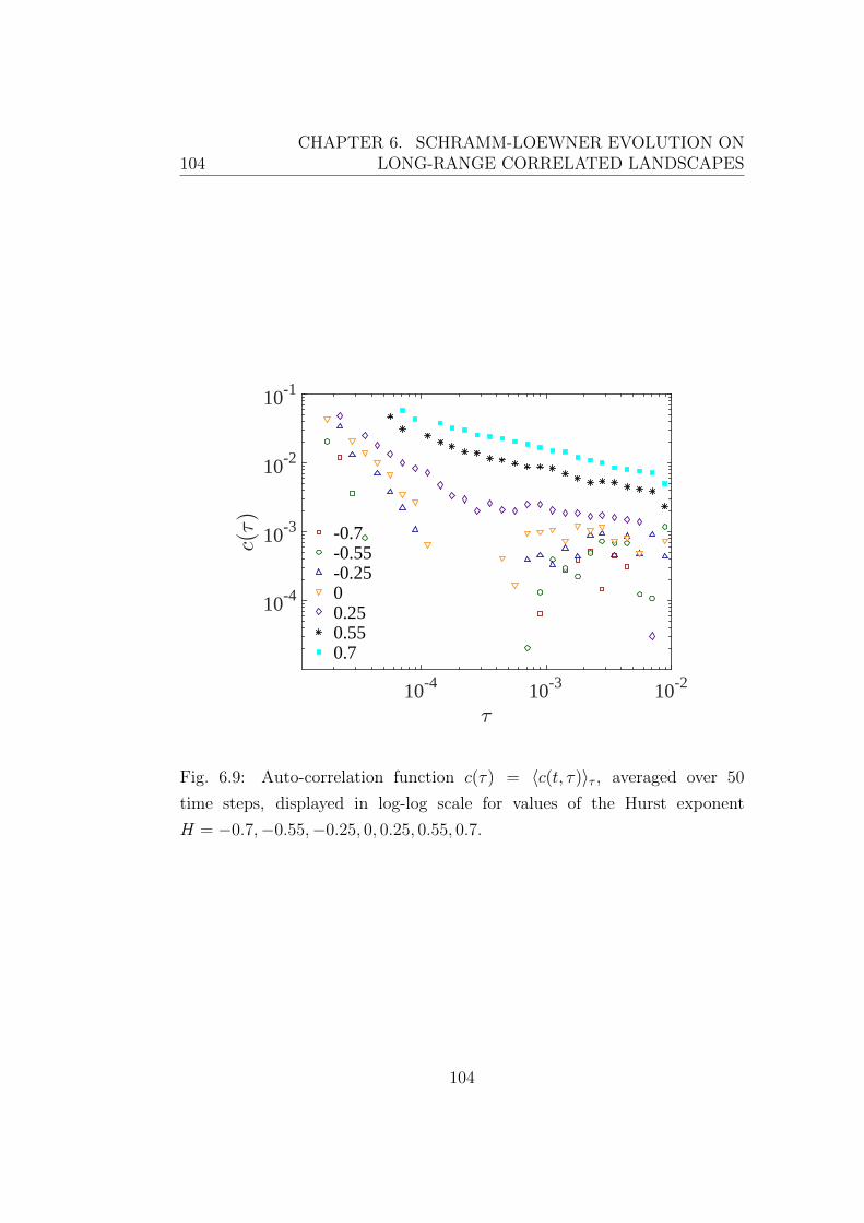
104CHAPTER 6. SCHRAMM-LOEWNER EVOLUTION ON
LONG-RANGE CORRELATED LANDSCAPES
=10-4 10-3 10-2
c(=)
10-4
10-3
10-2
10-1
-0.7-0.55-0.2500.250.550.7
Fig. 6.9: Auto-correlation function c(τ) = 〈c(t, τ)〉τ , averaged over 50
time steps, displayed in log-log scale for values of the Hurst exponent
H = −0.7,−0.55,−0.25, 0, 0.25, 0.55, 0.7.
104

6.5. OTHER CRITICAL CURVES 105
compatible with SLE for usual uncorrelated percolation in the case of the
shortest path, see Chapter 3, and uncorrelated landscapes in the case of
watersheds [30]. We want to check if these results still hold in the case
of long-range correlated percolation and long-range correlated landscapes.
Therefore, we compared the results obtained with the fractal dimension, the
winding angle, the direct SLE and in the case of watersheds also the left-
passage probability.
6.5.1 Winding angle measurements for the shortest
path and the watersheds
In Refs. [28, 99, 124, 147], the authors studied the dependence of the fractal
dimension of the shortest path and the watersheds on the value of the Hurst
exponent. Therefore we first test the compatibility between the variance of
the winding angle and the fractal dimension of the shortest path and the
watersheds for different values of the Hurst exponent. In the case of the
shortest path, the results are obtained on a triangular lattice with aspect
ratio one and H = −1,−0.85,−0.7,−0.55,−0.4,−0.25,−0.1, 0. In the case
of the watersheds, they are obtained on a square lattice of aspect ratio one
for H = −1, two for H = −0.8,−0.6,−0.5,−0.4,−0.2 and four for H = 0. In
Figs. 6.10 and 6.11, we show the rescaled variance of the winding angle for the
shortest path and the watersheds respectively. In both cases, the variance
σ2θ strongly depends on the value of the Hurst exponent H, see insets of
Figs. 6.10 and 6.11. In the case of the shortest path, for increasing values of
H, the linear regime is reached only for larger values of the vertical lattice
size Ly. This might be due to finite size effects, as the fractal dimension
of the curve is going to one, see Section 5.6, and therefore the variance of
the winding angle should converge to a constant, as displayed in the inset of
Fig. 6.10.
Using the relation df = 1 + κ8
and σ2θ = b + κ
4ln(Ly), one gets that σ2
θ =
b + 2(df − 1) ln(Ly) and obtains an estimate of the fractal dimension from
the variance of the winding angle. The results obtained by studying σ2θ give
estimates of the fractal dimension df in agreement with the directly measured
105
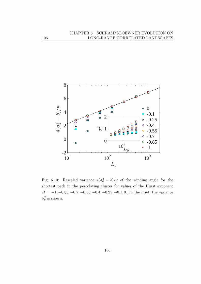
106CHAPTER 6. SCHRAMM-LOEWNER EVOLUTION ON
LONG-RANGE CORRELATED LANDSCAPES
Ly
101 102 103
4(<
2 3!
b)=5
-2
0
2
4
6
8
0-0.1-0.25-0.4-0.55-0.7-0.85-1Ly
102
<2 3
0
1
2
Fig. 6.10: Rescaled variance 4(σ2θ − b)/κ of the winding angle for the
shortest path in the percolating cluster for values of the Hurst exponent
H = −1,−0.85,−0.7,−0.55,−0.4,−0.25,−0.1, 0. In the inset, the variance
σ2θ is shown.
106
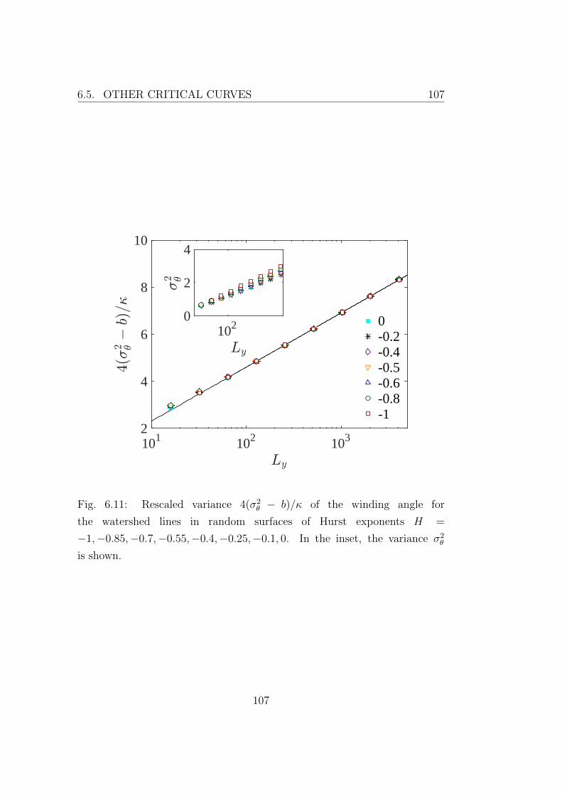
6.5. OTHER CRITICAL CURVES 107
Ly
101 102 103
4(<
2 3!
b)=5
2
4
6
8
10
0-0.2-0.4-0.5-0.6-0.8-1
Ly
102
<2 3
0
2
4
Fig. 6.11: Rescaled variance 4(σ2θ − b)/κ of the winding angle for
the watershed lines in random surfaces of Hurst exponents H =
−1,−0.85,−0.7,−0.55,−0.4,−0.25,−0.1, 0. In the inset, the variance σ2θ
is shown.
107

108CHAPTER 6. SCHRAMM-LOEWNER EVOLUTION ON
LONG-RANGE CORRELATED LANDSCAPES
1.0
1.1
1.2
-1.0 -0.8 -0.6 -0.4 -0.2 0.0
Fra
ctal
dim
ensi
on
df
Hurst exponent H
watershed w.a.watershed y.s.
shortest path w.a.shortest path y.s.
Fig. 6.12: Fractal dimension computed using the variance of the winding
angle (w.a.) compared with the fractal dimension measured using the yard-
stick method (y.s.) for the watershed lines and the shortest path in the cases
H = −1,−0.85,−0.7,−0.55,−0.4,−0.25,−0.1, 0. The black lines are the
conjectured dependence of the fractal dimension of the watersheds [28] and
the shortest path Eq. (5.17) on the value of the Hurst exponent H.
fractal dimension using the yardstick method, see Fig. 6.12.
6.5.2 Direct SLE test for the shortest path
In order to test if the results obtained with the winding angle measurements
are in agreement with SLE theory, we compute the variance of the driv-
ing function of the shortest path using the vertical slit map algorithm, see
Section 2.7.4. In Fig. 6.13, we see that, as expected from [31], in the uncor-
related case the variance of the driving function displays a linear behavior,
whereas in the correlated cases it is not linear anymore, but corresponds to
a superdiffusive process. Also, if one rescales the variance through the val-
108
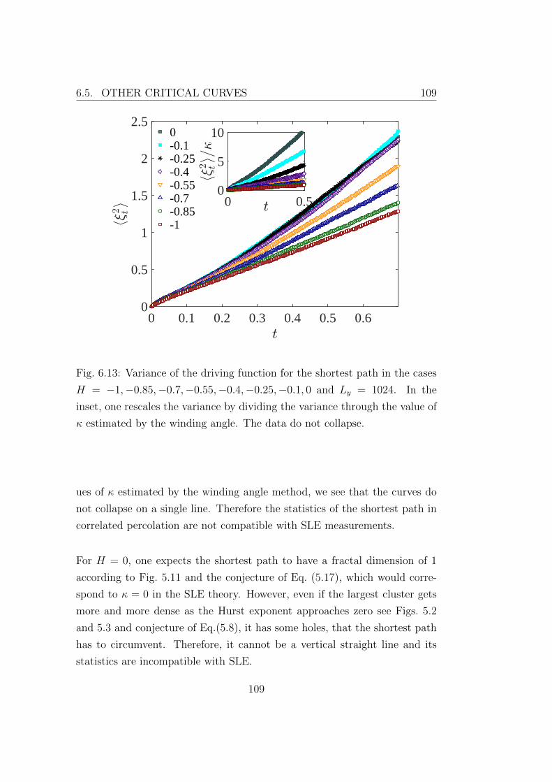
6.5. OTHER CRITICAL CURVES 109
t0 0.1 0.2 0.3 0.4 0.5 0.6
h92 ti
0
0.5
1
1.5
2
2.50-0.1-0.25-0.4-0.55-0.7-0.85-1
t0 0.5h9
2 ti=5
0
5
10
Fig. 6.13: Variance of the driving function for the shortest path in the cases
H = −1,−0.85,−0.7,−0.55,−0.4,−0.25,−0.1, 0 and Ly = 1024. In the
inset, one rescales the variance by dividing the variance through the value of
κ estimated by the winding angle. The data do not collapse.
ues of κ estimated by the winding angle method, we see that the curves do
not collapse on a single line. Therefore the statistics of the shortest path in
correlated percolation are not compatible with SLE measurements.
For H = 0, one expects the shortest path to have a fractal dimension of 1
according to Fig. 5.11 and the conjecture of Eq. (5.17), which would corre-
spond to κ = 0 in the SLE theory. However, even if the largest cluster gets
more and more dense as the Hurst exponent approaches zero see Figs. 5.2
and 5.3 and conjecture of Eq.(5.8), it has some holes, that the shortest path
has to circumvent. Therefore, it cannot be a vertical straight line and its
statistics are incompatible with SLE.
109

110CHAPTER 6. SCHRAMM-LOEWNER EVOLUTION ON
LONG-RANGE CORRELATED LANDSCAPES
t0 0.002 0.004 0.006 0.008 0.01
h92 ti
0
0.005
0.01
0.015
0-0.2-0.4-0.5-0.6-0.8-1
x=p
t-5 0 5
pt!
1P
(x)
0
0.2
Fig. 6.14: Variance of the driving function for the watershed lines in the cases
H = −1,−0.85,−0.7,−0.55,−0.4,−0.25,−0.1, 0 with Ly = 8192. In the
inset, the probability distribution of the driving function for a fixed Loewner
time is displayed for H = −1,−0.5, 0.
6.5.3 Direct SLE and left-passage probability for wa-
tersheds
We also compared the results obtained with the winding angle for watersheds
with the results obtained from the direct SLE and left-passage probability
measurements. In Fig. 6.14, the variance of the driving function is displayed,
along with the probability distribution of the driving function for a fixed
Loewner time. Contrary to the results obtained for the winding angle, in
Fig. 6.14 we do not see any clear dependence of the results of the variance of
the driving function on the value of the Hurst exponent. However, the auto-
correlation functions of the different driving functions displayed in Fig. 6.15
reveals that as soon as the landscape displays some correlations, i.e. H > −1,
the driving function displays long-range power-law time correlations, whereas
it is not the case for H = −1. Our results show that only in the case of
110
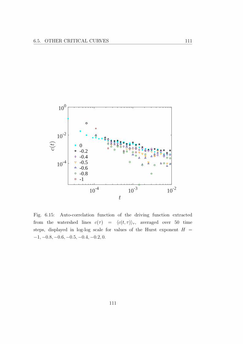
6.5. OTHER CRITICAL CURVES 111
t10-4 10-3 10-2
c(t)
10-4
10-2
100
0-0.2-0.4-0.5-0.6-0.8-1
Fig. 6.15: Auto-correlation function of the driving function extracted
from the watershed lines c(τ) = 〈c(t, τ)〉τ , averaged over 50 time
steps, displayed in log-log scale for values of the Hurst exponent H =
−1,−0.8,−0.6,−0.5,−0.4,−0.2, 0.
111
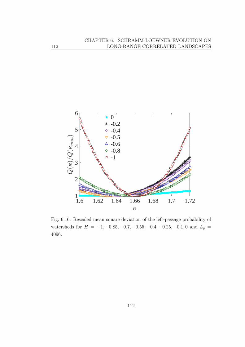
112CHAPTER 6. SCHRAMM-LOEWNER EVOLUTION ON
LONG-RANGE CORRELATED LANDSCAPES
51.6 1.62 1.64 1.66 1.68 1.7 1.72
Q(5
)=Q
(5m
in)
1
2
3
4
5
60-0.2-0.4-0.5-0.6-0.8-1
Fig. 6.16: Rescaled mean square deviation of the left-passage probability of
watersheds for H = −1,−0.85,−0.7,−0.55,−0.4,−0.25,−0.1, 0 and Ly =
4096.
112

6.5. OTHER CRITICAL CURVES 113
Hurst exponent H-1 -0.8 -0.6 -0.4 -0.2 0
Est
imate
d5
1
1.2
1.4
1.6
1.8
2
fract. dim.winding anglelppdSLE
Fig. 6.17: Estimated values of κ obtained with the fractal dimension (fract.
dim.), winding angle, left-passage probability (lpp) and direct SLE (dSLE)
measurements for H = −1,−0.85,−0.7,−0.55,−0.4,−0.25,−0.1, 0. The
black solid line corresponds to the value of κ deduced from the conjectured
dependence of the fractal dimension df on H [28], using κ(H) = 8(df (H)−1).
113

114CHAPTER 6. SCHRAMM-LOEWNER EVOLUTION ON
LONG-RANGE CORRELATED LANDSCAPES
uncorrelated landscapes, i.e. H = −1 watersheds have statistics compatible
with SLE, therefore recovering the result of Ref. [30].
We also did the left-passage probability measurement to estimate the value of
κ. We did not find a clear dependence of κ on the value of the Hurst exponent
H, see Fig. 6.16, as already seen for the direct SLE test. However we see
that the minimum is more pronouced for the value H = −1 corresponding
to the uncorrelated case. The results regarding watersheds are summarized
in Fig. 6.17.
6.6 Conclusion
We numerically showed that the statistics of the accessible perimeter of the
zero isoheight lines of Gaussian random landscapes are consistent with SLE
only for the range −1 ≤ H ≤ 0. Results for the fractal dimension, winding
angle and direct SLE are in agreement within error bars, see Fig. 6.4. How-
ever, for values of H near 0, we see strong finite-size effects, as expected from
the results presented in Section 5.3. This means that one can describe these
curves with a Brownian motion parametrized by a diffusivity κ.
In the two analytical limits H = −1 and H = 0, the complete perimeters are
SLE6 [29, 61] and SLE4 [35] respectively. From the duality relation, if the
complete perimeters are SLEκ the corresponding accessible perimeters are
SLEκ∗ with κκ∗ = 16 [11], see Section 2.5. Thus, in the analytical limits,
the accessible perimeters are SLE8/3 and SLE4 for H = −1 and H = 0
respectively, results that we recover in our numerical analysis.
To our knowledge, this is the first time that for an entire range of values of
the Hurst exponent H, a family of curves coupled to random landscapes is
shown to be SLE. This gives new insights in the field of fractional Gaussian
Fields in two dimensions [39] and suggests that this recent framework might
be helpful to understand correlated landscapes, see Section 4.4.
One might also wonder if these isoheight lines can be related to some random
walk process, as in the case of uncorrelated random landscapes and GFF.
For example, the isoheight lines for H = −1 and H = 0 are two specific
114

6.6. CONCLUSION 115
cases of the overruled harmonic walker [204] called respectively the critical
percolation exploration path [49, 205] and the harmonic explorer [71]. Our
work might provide insight for a future generalization of such walkers.
For isoheight lines in landscapes with positive Hurst exponent H > 0, we did
not find agreement with an SLE description of the curves. Even if we found
numerically that the driving function scales linearly in time, the driving
function displays power-law correlations, which contradicts the Markovian
properties of the driving function in the SLE theory. The results for both
positive and negative Hurst exponents are displayed in Fig. 6.18.
This work opens the possibility of applying SLE to the study of landscapes
with negative Hurst exponent H. As we have shown, many systems can be
considered from the point of view of a landscape, where isoheights play an
important role. Especially, it has been shown that zero vorticity isolines in
two-dimensional turbulence are SLE [32]. There have been also attempts to
extend this result to isolines in a generalized Navier-Stokes equation [34] to
study the conformal invariance of a larger class of turbulence problems. It
would be interesting to see if a relation between this problem and our results
can be drawn for the accessible perimeters of these contour lines.
We showed that, contrary to the case of the accessible perimeter, the shortest
path and the watershed line do not display statistics compatible with SLE
for H > −1, i.e when the system displays long-range correlations. In the
case of the shortest path, for −1 < H ≤ −3/4, from the numerical results,
it seems that the curve is no longer SLE, although there is no dependence of
the fractal dimension on the Hurst exponent H in this range.
115

116CHAPTER 6. SCHRAMM-LOEWNER EVOLUTION ON
LONG-RANGE CORRELATED LANDSCAPES
Hurst exponent H-1 -0.5 0 0.5 1
Est
imate
d5
0
2
4
6
8fract. dim.winding anglelppdSLE
Fig. 6.18: Estimated diffusion coefficients κ from the fractal dimension (fract.
dim.), the winding angle, the left-passage probability (lpp), and the direct
SLE (dSLE) methods for H ∈ [−1, 1]. The red crosses correpond to the
analytically known result for H = −1, i.e. percolation, and H = 0, i.e.
the GFF. We see that the results are compatible with SLE for H ≤ 0 but
incompatible for H > 0.
116

6.6. CONCLUSION 117
Pro
ble
mW
ind
ing
angl
eL
eft
Pass
age
Pro
b.
Dir
ect
SL
E
〈θ2〉
∼κ 4
ln(L
y)
Gau
ssia
nP
(θ)
κm
in=
minκQ
(κ)
Sch
ram
m’s
Pκ(φ
)
〈ξ2 t〉=
κt
Mark
ovia
nδξt
Gau
ssia
nξ t
WSH
=−
1Y
esX
Yes
Yes
Yes
Yes
Yes
SPH
=−
1Y
esY
esY
esY
esY
esY
esY
es
isoh
eigh
t
lin
esac
-
cess
ible
per
imet
er
H∈
[−1,
0]
Yes
Yes
Yes
Yes
Yes
Yes
Yes
isoh
eigh
t
lin
esac
-
cess
ible
per
imet
er
H∈
(0,1
]
Yes
,b
ut
slow
er
conve
rgen
cefo
r
larg
erva
lues
of
H
Yes
,b
ut
larg
er
dev
iati
onfo
r
larg
erva
lues
of
H
No,
no
stro
ng
dep
end
ence
on
Hfo
rκ
min
Yes
,b
ut
larg
erd
evi-
ati
on
sfr
om
Sch
ram
m’s
form
ula
for
incr
easi
ngH
No,
lin
ear
vari
an
ceb
ut
κdSLE
>4
inco
mp
ati
ble
wit
hdf<
3/2
No,
pow
er-l
aw
dec
rease
ofc(τ)
Yes
WS
H∈
(−1,
0]Y
esX
No,
no
dep
en-
den
ceonH
XN
o,
lin
ear
vari
-
an
ceb
ut
no
de-
pen
den
ceonH
No,
pow
er-l
aw
dec
rease
ofc(τ)
Yes
SP
H∈
(−1,
0]Y
esX
XX
No,
no
lin
ear
vari
an
ce
XX
Tab
le6.
1:S
um
mar
yof
the
resu
lts
obta
ined
for
the
wate
rsh
eds
(WS
),th
esh
ort
est
path
(SP
)an
dth
eis
oh
eight
lin
esw
ith
the
diff
eren
t
SL
Ete
sts:
the
win
din
gan
gle,
the
left
-pas
sage
pro
bab
ilit
yan
dth
ed
irec
tS
LE
test
s.F
or
the
win
din
gan
gle
test
,w
ete
sted
the
scali
ng
of
the
vari
ance
ofth
ew
ind
ing
angl
ean
dco
mp
ared
its
pro
bab
ilit
yd
istr
ibu
tion
wit
ha
Gau
ssia
nd
istr
ibu
tion
.F
or
the
left
-pass
age
pro
bab
ilit
y
test
,w
ees
tim
ated
theκ
from
the
min
imu
mof
the
mea
nsq
uare
dev
iati
on
an
dco
mp
are
dth
ele
ft-p
ass
age
pro
bab
ilit
ies
for
diff
eren
tp
oin
ts
inth
eu
pp
erh
alf-
pla
ne
wit
hS
chra
mm
’sfo
rmu
laE
q.
(2.2
6).
For
the
dir
ect
SL
Ete
st,
we
com
pu
ted
the
vari
an
ceof
the
dri
vin
gfu
nct
ion
,
its
Gau
ssia
nd
istr
ibu
tion
and
the
ind
epen
dan
ceof
its
incr
emen
ts.
Th
ete
sts
com
pati
ble
wit
hS
LE
are
den
ote
dby
’Yes
’(d
isp
laye
din
gree
n)
and
the
one
that
are
not
com
pat
ible
wit
ha
SL
Ed
escr
ipti
on
by
’No’
(dis
pla
yed
inre
d).
117

118CHAPTER 6. SCHRAMM-LOEWNER EVOLUTION ON
LONG-RANGE CORRELATED LANDSCAPES
H κfrac κθ κLPP κdSLE
−1 2.76± 0.16 2.66± 0.01 2.69± 0.08 2.66± 0.12
−0.85 2.80± 0.24 2.76± 0.02 2.80± 0.07 2.79± 0.10
−0.7 2.96± 0.24 2.94± 0.03 2.95± 0.11 2.97± 0.17
−0.55 3.20± 0.24 3.14± 0.03 3.13± 0.15 3.29± 0.32
−0.4 3.35± 0.31 3.32± 0.03 3.27± 0.17 3.46± 0.26
−0.25 3.64± 0.28 3.45± 0.09 3.40± 0.21 3.67± 0.26
−0.1 3.90± 0.18 3.49± 0.04 3.50± 0.24 3.84± 0.20
0 3.88± 0.20 3.44± 0.18 3.52± 0.25 3.98± 0.19
0.1 3.44± 0.40 3.34± 0.27 3.56± 0.26 4.07± 0.13
0.25 3.04± 0.24 3.07± 0.07 3.59± 0.29 4.26± 0.13
0.55 1.92± 0.24 2.22± 0.08 3.62± 0.36 4.84± 0.29
0.7 1.36± 0.16 1.65± 0.15 3.62± 0.41 5.35± 0.25
0.95 0.56± 0.16 0.62± 0.31 3.63± 0.50 5.97± 0.51
Table 6.2: For the isoheight lines: Diffusion coefficient κ computed from
the fractal dimension κfrac using data from [99] for H ≤ 0 and measured
using the yardstick method for H > 0, from the winding angle κθ, from
the left-passage probability κLPP and the direct SLE method κdSLE, for the
different values of the Hurst exponent H.
118
Chapter 7
Conformal Invariance in
Graphene
In the previous chapter, we have seen that isoheight lines in random surfaces
can display statistics compatible with SLE, but that for rough surfaces they
are not necessarily SLE. We studied the case of Gaussian random surfaces
with negative and positive Hurst exponent generated by the Fourier filtering
method.
In this Chapter we are interested in real surfaces simulated using molecu-
lar dynamics. In particular, the analysis of isoheight lines in the framework
of SLE might give insights into the conformal invariant properties of the
isoheight lines in real surfaces. In this Chapter we apply the SLE frame-
work to isoheight lines in Graphene. Due to thermal fluctuations, suspended
graphene sheets exhibit correlated random deformations. On these surfaces,
one can identify isoheight lines. We show that those lines, and the area
enclosed by them are fractal and that their fractal dimensions are indepen-
dant of temperature and system size, providing evidence for scale invariance
in graphene membranes. Furthermore, we provide numerical evidence that
these contour lines are conformally invariant by showing that they have the
same statistical properties as SLEκ curves with κ = 2.24± 0.07.
This Chapter in based on:
I. Giordanelli, N. Pose, M. Mendoza, and H. J. Herrmann, Conformal invari-
ance in graphene, in progress.
119
120 CHAPTER 7. CONFORMAL INVARIANCE IN GRAPHENE
7.1 Introduction
Graphene, consisting of literally a single carbon monolayer, represents the
first instance of a truly two-dimensional material [206–208]. The existence
of strictly two-dimensional crystals was first studied theoretically by Peierls
[209,210] and Landau [211,212], who demonstrated that, in the standard har-
monic approximation [213], thermal fluctuations should destroy long-range
order, resulting in melting of any 2D lattice at any finite temperature. Fur-
thermore, it was shown that crystalline order cannot exist in two dimen-
sions [214], due to the fact that long-wavelength fluctuations destroy the
long-range order of two-dimensional crystals, and suspended two-dimensional
membranes have a tendency to be crumpled [215]. Although the theory does
not permit the existence of perfect two-dimensional crystals, it allows the
existence of nearly perfect ones embedded in the three-dimensional space,
see Fig. 7.1. Indeed, a detailed analysis of the 2D crystal problem, beyond
the harmonic approximation, has led to the conclusion that atomically thin
membranes can be stabilised through their deformation in the third dimen-
sion [216–218].
Recently, it has been possible to construct experimentally suspended
graphene membranes, exhibiting random elastic deformations involving all
three dimensions [219]. The study of the structure of graphene membranes is
of great interest for the understanding of its electronic and mechanical prop-
erties. For instance, it has been shown that reducing the standard deviation
of the heights increases the electronic mobility, and consequently increases the
electrical conductivity [220]. Furthermore, the structure of the membranes
can lead to fluctuations of the charge density and thus to the formation of
electron and hole valleys (puddles) in globally neutral samples. The existence
of stable rippled graphene membranes and the interplay between thermal
fluctuations and anharmonic coupling between bending and stretching modes
open up the question whether suspended graphene can be studied within the
theory of critical phenomena, where scale and conformal invariance play an
important role. Conformal invariance is a very powerful property to classify
theoretical models and gain insights into physical systems [165,221–223]. In
120

7.1. INTRODUCTION 121
Fig. 7.1: Graphene membrane after thermalisation. Inset: The blue points
represent carbon atoms that are above the isoheight plane. The red line
shows the extracted path along the intersection between the membrane and
the isoheight plane.
121

122 CHAPTER 7. CONFORMAL INVARIANCE IN GRAPHENE
recent years, the SLE theory has become a very useful numerical tool to in-
vestigate conformal invariance of many physical systems. This is due to the
fact that random curves that are SLE are necessarily conformally invariant.
Although SLE was primarily developed to describe analytically curves in sta-
tistical models on lattices at criticality [29–31, 35, 48, 60, 61, 69, 70, 224, 225],
it has been successfully applied to other systems such as two-dimensional
turbulence [32], isoheight lines in growth models [226], and experimentally
grown surfaces [37]. Conformal invariant curves also possess special statisti-
cal properties of their winding angle, see Section 2.7.2. Our goal is to find out
whether scale and conformal invariance are properties of isoheight contour
lines of graphene membranes.
7.2 Methodology
Here we simulate graphene membranes using molecular dynamics with the
adaptive intermolecular reactive bond-order (AIREBO) potential [227]. The
AIREBO potential can be represented by a sum over pairwise interactions,
which includes the covalent bonding interactions, a torsion term, guarantee-
ing the correct dihedral angles, and a Lennard-Jones term, which describes
the non-bonded interaction between the atoms. This many-body potential
describes properly graphene membranes [228].
We have performed simulations of graphene membranes of size 200A×200A,
400A × 400A, and 800A × 800A, at different temperatures, i.e. 100 K, 300
K, and 600 K. The simulation time step has been set to one fs, which is
sufficiently small to capture the carbon-carbon interactions. We let the sam-
ples evolve for over 1.4 ns, 3 ns, and 13 ns, for system sizes 800A × 800A,
400A×400A, and 200A×200A, respectively. In order to control the temper-
ature, we have applied the Nose-Hoover thermostat. Each simulation starts
with a flat graphene membrane located in the x−y plane with a small random
perturbation in z-direction, to break the symmetry in the z-direction, and
zero initial velocity, i.e. zero temperature. For each temperature and sys-
tem size we performed three independent simulations with different random
122

7.3. SCALE INVARIANCE IN GRAPHENE 123
seeds for the initial fluctuations. In order to accelerate the thermalisation
of the graphene membrane, we heat up the membrane gradually. We use an
equilibration time of 0.2 ns to reach the desired temperature.
From each simulation, we extract graphene sheets in intervals of 5 ps, to avoid
correlated samples. By using this procedure, we obtain for each temperature
up to 720, 1680, and 7680 graphene sheets for 800A × 800A, 400A × 400A,
and 200A× 200A, respectively.
7.3 Scale invariance in graphene
Once the samples have reached the thermal equilibrium, we first study the
height-height correlations, see Section 4.2. For numerical convenience, in-
stead of working with the height-height correlation function c(r) = 〈h(x +
r)h(x)〉, one works with the function H(r) = 〈(h(x + r)− h(x))2〉 =
2〈h(x)2〉 − 2c(r), where h denotes the local height of the graphene mem-
brane. For self-affine surfaces, the function H(r) exhibits a power-law be-
haviour, i.e. H(|r|) ∝ |r|2H , where the exponent H is the so-called Hurst
exponent and characterises the roughness of the surface, see Subsection 4.2.
We have performed the statistical averages 〈...〉 by taking the carbon atoms
inside the inner half of the graphene membrane to avoid boundary effects.
In particular, this allows us to neglect the curvature of the sheet that might
arrise at the boundary of the sheet, where some crumpling can appear. All
the measurements have been done on the inner half of the surface.
The results presented in Fig. 7.2 indicate that the Hurst exponent is both
independent of system size and independent of temperature within error bars.
The obtained Hurst exponent is H = 0.72 ± 0.01. Our results are in good
agreement with the Hurst exponent measured by Adedpour et al. [229], where
it was found 0.6 < H < 0.74. The existence of a Hurst exponent suggests
that graphene membranes are self-affine surfaces.
The contour lines of self-affine surfaces often exhibit scale-invariance, as it is
the case for random Gaussian surfaces [12]. Assuming that we only consider
atoms of the graphene membrane that are above a certain height, and starting
123
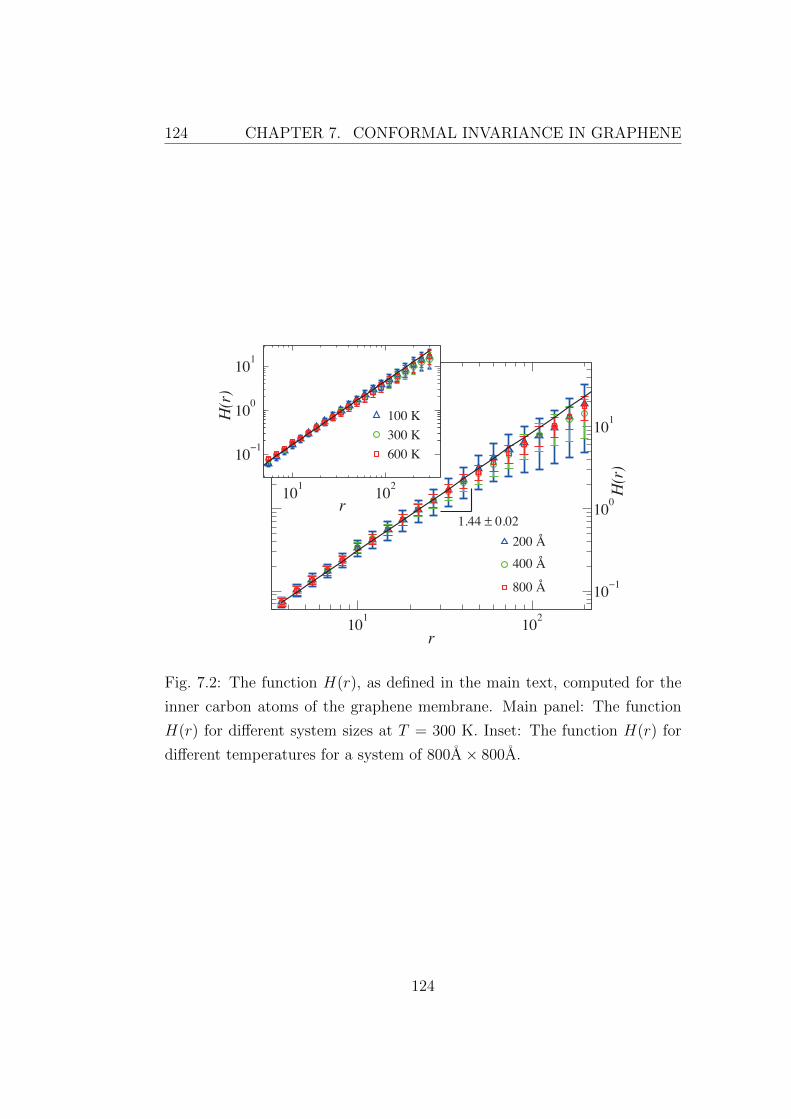
124 CHAPTER 7. CONFORMAL INVARIANCE IN GRAPHENE
101
102
10−1
100
101
r
H(r)
101
102
100
101
10−1
r
H(r)
100 K
300 K
600 K
1.44 ± 0.02
200 Å
400 Å
800 Å
Fig. 7.2: The function H(r), as defined in the main text, computed for the
inner carbon atoms of the graphene membrane. Main panel: The function
H(r) for different system sizes at T = 300 K. Inset: The function H(r) for
different temperatures for a system of 800A× 800A.
124
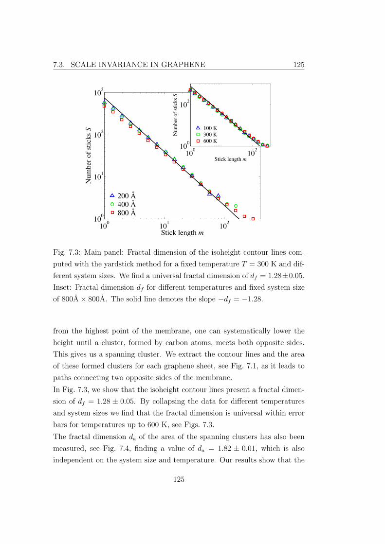
7.3. SCALE INVARIANCE IN GRAPHENE 125
100
101
10210
0
101
102
103
Stick length m
Num
ber
of s
ticks
S
200 Å400 Å800 Å
100
10210
0
102
Stick length m
Num
ber
of s
ticks
S
100 K300 K600 K
Fig. 7.3: Main panel: Fractal dimension of the isoheight contour lines com-
puted with the yardstick method for a fixed temperature T = 300 K and dif-
ferent system sizes. We find a universal fractal dimension of df = 1.28±0.05.
Inset: Fractal dimension df for different temperatures and fixed system size
of 800A× 800A. The solid line denotes the slope −df = −1.28.
from the highest point of the membrane, one can systematically lower the
height until a cluster, formed by carbon atoms, meets both opposite sides.
This gives us a spanning cluster. We extract the contour lines and the area
of these formed clusters for each graphene sheet, see Fig. 7.1, as it leads to
paths connecting two opposite sides of the membrane.
In Fig. 7.3, we show that the isoheight contour lines present a fractal dimen-
sion of df = 1.28 ± 0.05. By collapsing the data for different temperatures
and system sizes we find that the fractal dimension is universal within error
bars for temperatures up to 600 K, see Figs. 7.3.
The fractal dimension da of the area of the spanning clusters has also been
measured, see Fig. 7.4, finding a value of da = 1.82 ± 0.01, which is also
independent on the system size and temperature. Our results show that the
125

126 CHAPTER 7. CONFORMAL INVARIANCE IN GRAPHENE
101
102
103
104
r
N
101
102
102
104
103
r
N
100 K
300 K
600 K
1.82 ± 0.01
200 Å
400 Å
800 Å
Fig. 7.4: Fractal dimension of the area enclosed by the isoheight contour
lines of the spanning clusters, computed with the box counting method. The
number N of boxes used to cover the atoms belonging to the spanning cluster
is displayed as a function of the lateral size r of the boxes. Main panel: Box
counting method for different system sizes at T = 300 K. Inset: Box counting
method for different temperatures for a system size of 800A× 800A.
isoheight contour lines of the spanning cluster and the area enclosed by them
possess scale invariant properties.
7.4 Conformal invariance and SLE properties
in graphene
Let us study the conformal invariance of the isoheight contour lines. A family
of random curves is said to be conformally invariant if their statistics is con-
served by conformal transformations, see Section 2.5. This property allows to
make analytical developments toward the solution of complex problems [165].
126
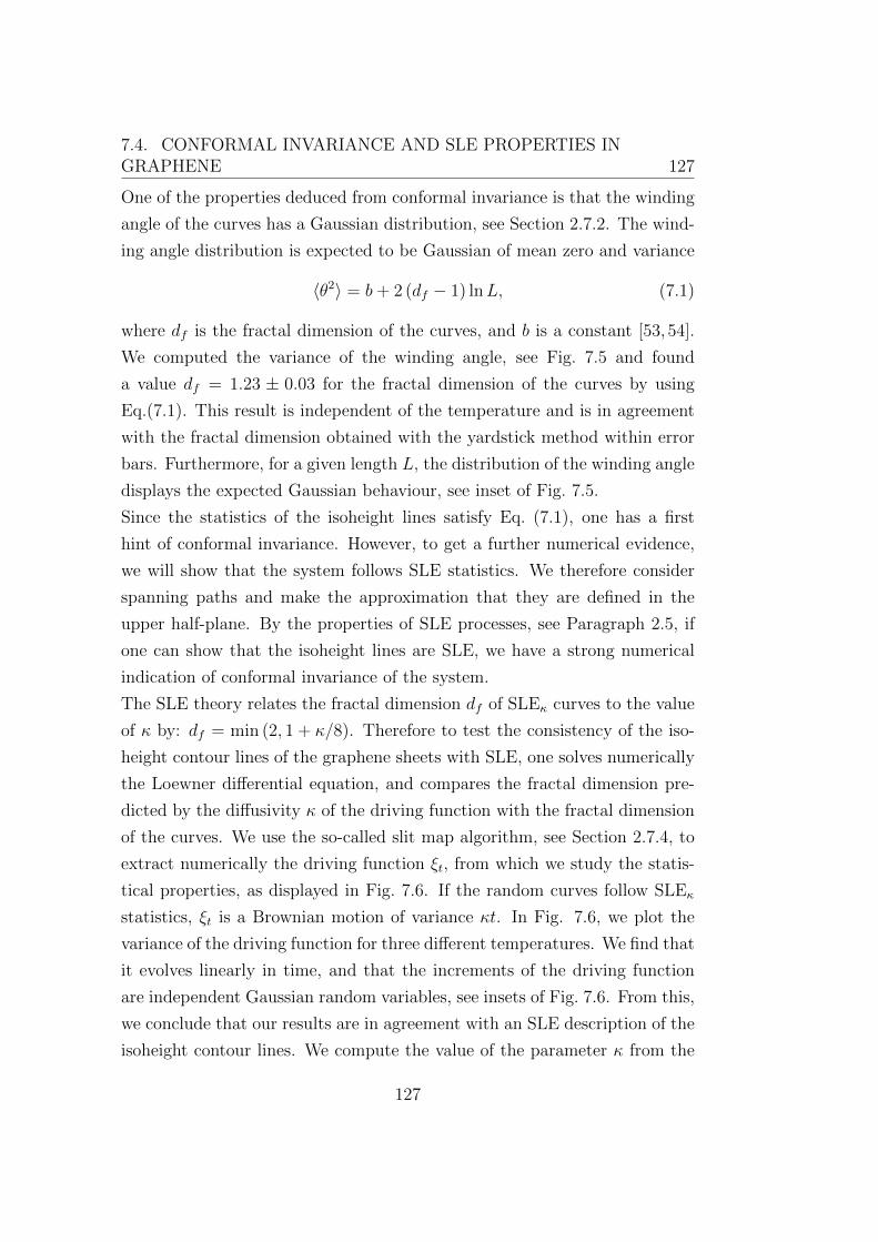
7.4. CONFORMAL INVARIANCE AND SLE PROPERTIES INGRAPHENE 127
One of the properties deduced from conformal invariance is that the winding
angle of the curves has a Gaussian distribution, see Section 2.7.2. The wind-
ing angle distribution is expected to be Gaussian of mean zero and variance
〈θ2〉 = b+ 2 (df − 1) lnL, (7.1)
where df is the fractal dimension of the curves, and b is a constant [53, 54].
We computed the variance of the winding angle, see Fig. 7.5 and found
a value df = 1.23 ± 0.03 for the fractal dimension of the curves by using
Eq.(7.1). This result is independent of the temperature and is in agreement
with the fractal dimension obtained with the yardstick method within error
bars. Furthermore, for a given length L, the distribution of the winding angle
displays the expected Gaussian behaviour, see inset of Fig. 7.5.
Since the statistics of the isoheight lines satisfy Eq. (7.1), one has a first
hint of conformal invariance. However, to get a further numerical evidence,
we will show that the system follows SLE statistics. We therefore consider
spanning paths and make the approximation that they are defined in the
upper half-plane. By the properties of SLE processes, see Paragraph 2.5, if
one can show that the isoheight lines are SLE, we have a strong numerical
indication of conformal invariance of the system.
The SLE theory relates the fractal dimension df of SLEκ curves to the value
of κ by: df = min (2, 1 + κ/8). Therefore to test the consistency of the iso-
height contour lines of the graphene sheets with SLE, one solves numerically
the Loewner differential equation, and compares the fractal dimension pre-
dicted by the diffusivity κ of the driving function with the fractal dimension
of the curves. We use the so-called slit map algorithm, see Section 2.7.4, to
extract numerically the driving function ξt, from which we study the statis-
tical properties, as displayed in Fig. 7.6. If the random curves follow SLEκ
statistics, ξt is a Brownian motion of variance κt. In Fig. 7.6, we plot the
variance of the driving function for three different temperatures. We find that
it evolves linearly in time, and that the increments of the driving function
are independent Gaussian random variables, see insets of Fig. 7.6. From this,
we conclude that our results are in agreement with an SLE description of the
isoheight contour lines. We compute the value of the parameter κ from the
127
128 CHAPTER 7. CONFORMAL INVARIANCE IN GRAPHENE
Endpoint distance L10
1
0
0.5
1
1.5
2
〈θ〉
〈θ2〉
100 K
300 K
600 K
θ/〈θ2〉1/2-2 0 2
〈θ2〉−
1/2P(θ)
10-2
10-1
Fig. 7.5: Main panel: Mean 〈θ〉 and variance 〈θ2〉 of the winding angle θ
of the isoheight contour lines for three different temperatures T = 100 K,
T = 300 K, and T = 600 K, in a semi-log plot. The mean is approximately
zero and the variance linear in lnL. The solid line denotes the best fitting.
Inset: Rescaled probability distribution of the winding angle for L = 13.37
A, compared to a Gaussian distribution of variance one (solid line).
128

7.4. CONFORMAL INVARIANCE AND SLE PROPERTIES INGRAPHENE 129
t
0 50 100 150 200
〈ξ2 t〉−
〈ξt〉2
0
100
200
300
400
500
100K
300K
600K
x
-20 0 20
P(x)
0
0.2
t0 100
C(t)
-1
0
1
Fig. 7.6: Main panel: Variance of the driving function 〈ξ2t 〉 for three different
temperatures T = 100 K, 300 K, 600 K. The solid line shows the linear depen-
dence of the variance of a driving function with diffusivity κ = 2.24. Upper-
left inset: the probability distribution of the driving function at t = 29. The
solid line is the probability distribution of a Gaussian random variable of zero
mean and variance 2.24. Bottom-right inset: The autocorrelation function
of the increments of the driving function, averaged over the range t = 29 to
49.
129

130 CHAPTER 7. CONFORMAL INVARIANCE IN GRAPHENE
51 1.5 2 2.5 3 3.5 4
Q(5
)=Q
min
2
4
6
8
10
100K300K600K
3=:0 0.5 1
P5(3
)
0
0.5
1
Fig. 7.7: Measured rescaled mean square deviation Q(κ)/Qmin as a function
of κ with Qmin the minimum value of Q, for temperatures T = 100K, T =
300K, and T = 600K. Inset: the measured left-passage probabilities are
compared with Schramm’s formula for κ = 2.24 (displayed as the solid line).
variance of the driving function for three different temperatures obtaining
κ = 2.24 ± 0.07. This result implies a fractal dimension of ∼ 1.28, which is
in good agreement with the fractal dimension of the curves measured with
both, the yardstick method and the winding angle. Note that the value of
the diffusion coefficient κ is independent of the temperature. We also checked
that the left-passage probability of the curves can be described by Schramm’s
formula, see Fig. 7.7, and estimated the value of κ to be κ = 2.27 ± 0.08.
In the inset of Fig. 7.7, we show that the left-passage probability satisfies
Schramm’s formula (2.26).
130
7.5. DIFFERENCE BETWEEN GRAPHENE SHEETS AND GAUSSIANRANDOM SURFACES 131
7.5 Difference between graphene sheets and
Gaussian random surfaces
As we have shown before, graphene sheets are rough surfaces characterized
by a positive Hurst exponent H = 0.72±0.01. However, as we have shown in
Section 6.3, Gaussian random surfaces with positive Hurst exponent and free
boundary conditions do not display statistics compatible with SLE. Also their
isoheights have different fractal dimensions. This suggests that graphene
sheets are not Gaussian random surfaces, therefore we will need to further
study the difference between graphene sheets and the random surfaces gen-
erated with the Fourier filtering method.
First, from a qualitative point of view, Gaussian random surfaces and
graphene sheets look differently. As characterized by Kalda in Ref. [14],
rough surfaces with H ∈ [0, 1) display peaks of different sizes and the heights
of the surfaces are expected to be unbounded, see for example Fig. 4.2(d),
whereas for graphene sheets you do not expect the surface do display peaks
of unbounded sizes, see Fig. 7.1, as the number of atoms is finite and very
strong peaks are expected to crumple the surface.
From a quantitative point of view, the difference of the fractal dimensions
of the isoheight lines between graphene and the Gaussian random surface
shows that these two surfaces display different statistical properties. In order
to further study this point, we make a Fourier analysis of graphene surfaces
and study them within the framework of random surfaces. In particular, we
investigate the properties of the Fourier coefficients uq = |uq|eiφq , and in
particular their phase φq, and modulus |uq|. By studying the distribution of
the modulus, see Fig. 7.8, we have found that graphene sheets and Gaussian
random surfaces generated with the Ffm display different distribution of the
modulus, even though both phases are uniformly distributed. This might
lead to the property that isoheight lines display SLE statistics although we
would need further studies to conclude. For example, one has to study the
independence of the Fourier coefficients, especially that the phases of the
131
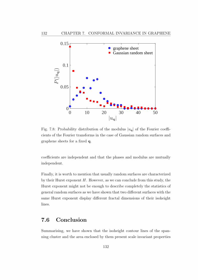
132 CHAPTER 7. CONFORMAL INVARIANCE IN GRAPHENE
juqj0 10 20 30 40 50
P(ju
qj)
0
0.05
0.1
0.15graphene sheetGaussian random sheet
Fig. 7.8: Probability distribution of the modulus |uq| of the Fourier coeffi-
cients of the Fourier transforms in the case of Gaussian random surfaces and
graphene sheets for a fixed q.
coefficients are independent and that the phases and modulus are mutually
independent.
Finally, it is worth to mention that usually random surfaces are characterized
by their Hurst exponent H. However, as we can conclude from this study, the
Hurst exponent might not be enough to describe completely the statistics of
general random surfaces as we have shown that two different surfaces with the
same Hurst exponent display different fractal dimensions of their isoheight
lines.
7.6 Conclusion
Summarising, we have shown that the isoheight contour lines of the span-
ning cluster and the area enclosed by them present scale invariant properties
132
7.6. CONCLUSION 133
independent of the temperature within the range of 100-600 K. Furthermore
using four different numerical tests, we have shown the the isoheight contour
lines of the spanning cluster are conformal invariant and can be described
by SLEκ with κ = 2.24 ± 0.08. Also we have shown that the Hurst expo-
nent is not enough to characterize fully the statistics of the isoheight lines
of random surfaces. The influence of other parameters on the statistics of
the random surfaces should be further studied, like the influence of proba-
bility distribution of the modulus and the correlations between the Fourier
coefficients.
The fact that the isoheight lines are conformal invariant relates the study
of graphene with other critical phenomena in two dimensions, like percola-
tion, and other phenomenas like turbulence [32], and opens up the question
whether there are additional shared properties that can help to understand
the physical properties of graphene.
The consequences of our findings to the electronic mobility in graphene will
be a subject of future research. Furthermore, an open question remains,
whether the scale and conformal invariant properties are typical for graphene
or are also exhibited by other two-dimensional crystals. We have made tests
on suspended silicene, a membrane made with silicon atoms, and we have
found that it crumples, preventing us to perform the same analysis.
133
134 CHAPTER 7. CONFORMAL INVARIANCE IN GRAPHENE
134
Chapter 8
Discussion and Outlook
Schramm-Loewner Evolution is a very recent and successful mathematical
theory to describe Statistical Physics models, which has allowed to compute
exactly critical exponents. The SLE theory gives not only insights into crit-
ical exponents but also into the probability distribution of curves, allowing
for example to compute the probability for given points to be at the left or
at the right of a random curve obeying SLE statistics. In this thesis, we
studied this theory and applied it to different problems like the shortest path
in percolation, long-range correlated percolation, and graphene.
Some complex optimisation problems like computing the shortest path, as
we have studied in Chapter 3, have been shown to be analytically difficult
to track using common Statistical Physics tools. Many conjectures have
been proposed, which have all been ruled out. Therefore, the consistency
of the statistics of the shortest path in percolation with SLE opens a new
possibility to tackle the long-standing problem of its fractal dimension by
using this theory.
Recently, physicists and mathematicians have been interested in the coupling
between isoheight lines and random surfaces. It is a very promising field and
has triggered a lot of studies on the SLE properties of the isoheight lines on
these surfaces. Even if mathematically only two surfaces have been proven to
have isoheight lines obeying SLE properties, the uniformly random surface
and the Gaussian Free Field (GFF), physicists have shown empirically or nu-
135
136 CHAPTER 8. DISCUSSION AND OUTLOOK
merically that isoheight lines in real surfaces can display statistics compatible
with SLE.
In Chapter 5 we studied the critical properties of long-range correlated per-
colation characterized by the Hurst exponent H. We studied the dependence
of the fractal dimension of the percolating cluster and showed that it be-
comes more compact for increasing values of H. We also studied the cluster
size distribution at criticality and its dependence on H. Moreover the fractal
dimension of the complete and accessible perimeters of the largest cluster
were studied and found to satisfy the duality relation for every value of H.
For increasing values of H, the fractal dimension of the shortest path was
found to be decreasing towards 1, and the conductivity exponent was found
to sharply decrease for H going to 0. These results are in agreement with the
backbone of the largest cluster getting more compact for increasing H. We
also proposed quantitative relations on the dependence of the studied critical
exponents on H.
In Chapter 6, we numerically showed that the statistics of the accessible
perimeter of the zero isoheight lines of Gaussian random landscapes are con-
sistent with SLE only for −1 ≤ H ≤ 0 and not for 0 < H < 1, and recovered
the analytical results in the limiting cases H = −1 and H = 0. To our
knowledge, this is the first time that for an entire range of values of the
Hurst exponent H, a family of curves coupled to their random landscapes
is shown to be compatible with SLE. This result opens the possibility of
applying SLE to the study of landscapes with negative Hurst exponent H
within the framework of fractional Gaussian fields. Contrary to the case of
the accessible perimeter, for watersheds and the shortest path, we did not
find agreement with SLE statistics as soon as correlations were introduced
in the system, i.e. for H > −1.
In Chapter 7, we studied the properties of graphene sheets as rough sur-
faces. This allowed us to show that, for a wide range of temperatures, the
sheets display not only scale invariance but also conformal invariance. We
computed their Hurst exponent and the fractal dimension of their isoheight
136

137
lines. We also showed numerically that the statistics of the winding angle are
compatible with predictions from conformal invariance and that the isoheight
lines even display statistics compatible with SLE. Comparing with results ob-
tained in Chapter 6, we have shown that the Hurst exponent is not enough
to characterize fully the statistical properties of isoheight lines on general
rough surfaces, which opens up the question of the best characterization of
rough surfaces to describe fully the statistics of random landscapes.
As the analytical analysis of random processes from Statistical Physics using
SLE is difficult to tackle, numerical analysis of random processes like the
shortest path in percolation gives interesting insights into the field of appli-
cations of SLE. Numerical results and conjectures show that SLE has more
applications than the few rigorously proven cases, and might successfully de-
scribe scaling limits of the Loop-Erased Random Walk, Potts model, spin
glasses, watersheds, the shortest path in percolation and accessible hulls in
correlated percolation. Therefore further studies in these fields could lead
to interesting results, and in the case of the shortest path lead to the ex-
act computation of one of the last critical exponent, whose exact value is
unknown.
SLE related to random surfaces has gained an increasing interest, from a
numerical and theoretical points of view. The coupling between SLE and
random surfaces has many implications in physical systems like graphene,
turbulence, or grown surfaces. Much work can be done in characterizing ran-
dom surfaces and their coupling with SLE. Here we focused on Gaussian ran-
dom surfaces with negative Hurst exponent and suspended Graphene sheets.
But other kind of surfaces, especially displaying non Gaussian statistics, or
with other type of correlations, like correlations between the phases in the
Fourier coefficients of the Fourier transformed surface, could be studied to
better understand the coupling between SLE and real surfaces. As we have
seen in the case of Graphene sheets, real surfaces are not always Gaussian
random surfaces. Also, the Hurst exponent is not be enough to characterize
fully the properties of the random surfaces, and other parameters should be
taken into account to describe better the properties of the surface. Also,
137

138 CHAPTER 8. DISCUSSION AND OUTLOOK
the interplay between random walkers and random surfaces could lead to
interesting characterizations of surfaces. In the case of the GFF, a relation
between the GFF and a random walker has been made. Studying this relation
for other surfaces could lead to interesting developments.
Interesting results have been proven by extending the SLE theory to other
driving functions in order to describe new kinds of processes like biased or
branching processes for example. This can be done by changing the driving
function, adding a drift term to the usual Brownian motion in the SLE(κ, ρ)
theory [59, 230] or replacing for example the Brownian motion by Levy pro-
cesses [231, 232] to describe branching, or even by changing the derivative
operator in the Loewner Equation [233]. However we have seen that in some
of the studied cases, like in the case of watersheds for correlated surfaces, the
underlying driving process displays correlations. Studying correlated pro-
cesses might give interesting insights into some common Statistical Physics
problems and lead to new results.
138

References
[1] G. F. Lawler. Conformally Invariant Processes in the Plane, volume
114. Mathematical Surveys and Monographs, 2005.
[2] M. E. J. Newman and R. M. Ziff. Efficient Monte Carlo algorithm and
high-precision results for percolation. Phys. Rev. Lett., 85:4104, 2000.
[3] M. E. J. Newman and R. M. Ziff. Fast Monte Carlo algorithm for site
or bond percolation. Phys. Rev. E, 64:016706, 2001.
[4] J. Hoshen and R. Kopelman. Percolation and cluster distribution.
I. Cluster multiple labeling technique and critical concentration algo-
rithm. Phys. Rev. B, 14:3438, 1976.
[5] R. F. Voss. The fractal dimension of percolation cluster hulls. J. Phys.
A, 17:L373, 1984.
[6] B. Sapoval, M. Rosso, and J. F. Gouyet. The fractal nature of a dif-
fusion front and the relation to percolation. J. Phys. Lett., 46:L149,
1985.
[7] P. Grassberger. On the hull of two-dimensional percolation clusters. J.
Phys. A, 19:2675, 1986.
[8] T. Grossman and A. Aharony. Accessible external perimeters of per-
colation clusters. J. Phys. A, 20:L1193, 1987.
[9] H. Saleur and B. Duplantier. Exact determination of the percolation
hull exponent in two dimensions. Phys. Rev. Lett., 58:2325, 1987.
139
140 REFERENCES
[10] M. Aizenman, B. Duplantier, and A. Aharony. Path-crossing exponents
and the external perimeter in 2D percolation. Phys. Rev. Lett., 83:1359,
1999.
[11] B. Duplantier. Conformally Invariant Fractals and Potential Theory.
Phys. Rev. Lett., 84:1363, 2000.
[12] J. Kondev and C. L. Henley. Geometrical Exponents of Contour Loops
on Random Gaussian Surfaces. Phys. Rev. Lett., pages 4580–4583,
1995.
[13] J. Kalda. Description of random Gaussian surfaces by a four-vertex
model. Phys. Rev. E, 64:020101(R), 2001.
[14] J. Kalda. Statistical topography of rough surfaces: “oceanic coastlines”
as generalizations of percolation clusters. EPL, 84:46003, 2008.
[15] I. Mandre and J. Kalda. Monte-Carlo study of scaling exponents of
rough surfaces and correlated percolation. Eur. Phys. J. B, 83:107,
2011.
[16] W. Janke and A. M. J. Schakel. Geometrical vs. Fortuin-Kasteleyn
clusters in the two-dimensional q-state Potts model. Nucl. Phys. B,
700:385, 2004.
[17] H. J. Herrmann, D. C. Hong, and H. E. Stanley. Backbone and elas-
tic backbone of percolation clusters obtained by the new method of
’burning’. J. Phys. A, 17:L261–L266, 1984.
[18] H. J. Herrmann and H. E. Stanley. The fractal dimension of the min-
imum path in two- and three-dimensional percolation. J. Phys. A,
21:L829–L833, 1988.
[19] P. Grassberger. Spreading and backbone dimension of 2D percolation.
J. Phys. A, 25:5475–5484, 1992.
140
REFERENCES 141
[20] Z. Zhou, J. Yang, Y. Deng, and R. M. Ziff. Shortest-path fractal
dimension for percolation in two and three dimensions. Phys. Rev. E,
86:061101, 2012.
[21] H. A. Makse, S. Havlin, P. C. Ivanov, P. R. King, S. Prakash, and
H. E. Stanley. Pattern formation in sedimentary rocks: Connectivity,
permeability and spatial correlations. Physica A, 233:587, 1996.
[22] S. Prakash, S. Havlin, M. Schwartz, and H. E. Stanley. Structural and
dynamical properties of long-range correlated percolation. Phys. Rev.
A, 46:R1724, 1992.
[23] H. J. Herrmann and H. E. Stanley. Building blocks of percolation
clusters: Volatile fractals. Phys. Rev. Lett., 53:1121–1124, 1984.
[24] M. D. Rintoul and H. Nakanishi. A precise determination of the back-
bone fractal dimension on two-dimensional percolation clusters. J.
Phys. A, 25:L945, 1992.
[25] P. Grassberger. Pair connectedness and the shortest-path scaling in
critical percolation. J. Phys. A, 32:6233–6238, 1999.
[26] Y. Deng, H. W. J. Blote, and B. Nienhuis. Backbone exponents of the
two-dimensional q-state Potts model: A Monte Carlo investigation.
Phys. Rev. E, 69:026114, 2004.
[27] J. Kondev, C. L. Henley, and D. G. Salinas. Nonlinear measures for
characterizing rough surface morphologies. Phys Rev. E, 61:104–125,
2000.
[28] K. J. Schrenk. Discontinuous percolation transitions and lattice models
of fractal boundaries and paths. ETH Zurich, Zurich, diss. eth no. 21669
edition, 2014.
[29] O. Schramm. Scaling limits of loop-erased random walks and uniform
spanning trees. Isr. J. Math., 118:221–288, 2000.
141
142 REFERENCES
[30] E. Daryaei, N. A. M. Araujo, K. J. Schrenk, S. Rouhani, and H. J.
Herrmann. Watersheds are Schramm-Loewner evolution curves. Phys.
Rev. Lett., 109:218701, 2012.
[31] N. Pose, K. J. Schrenk, N. A. M. Araujo, and H. J. Herrmann. Shortest
path and Schramm-Loewner Evolution. Sci. Rep., 4:5495, 2014.
[32] D. Bernard, G. Boffetta, A. Celani, and G. Falkovich. Conformal in-
variance in two-dimensional turbulence. Nat. Phys., 2:124–128, 2006.
[33] D. Bernard, G. Boffetta, A. Celani, and G. Falkovich. Inverse turbulent
cascades and conformally invariant curves. Phys. Rev. Lett., 98:024501,
2007.
[34] G. Falkovich and S. Musacchio. Conformal Invariance in Inverse Tur-
bulent Cascades.
[35] O. Schramm and S. Sheffield. Contour lines of the two-dimensional
discrete Gaussian free field. Acta. Math., 202:21–137, 2009.
[36] O. Schramm and S. Sheffield. A contour line of the continuum Gaussian
free field. Probab. Theory Relat. Fields, 157:47–80, 2013.
[37] A. A. Saberi, M. A. Rajabpour, and S. Rouhani. Conformal Curves on
the WO3 Surface. Phys. Rev. Lett., 100:044504, 2008.
[38] A. A. Saberi, M. D. Niry, S. M. Fazeli, M. R. Rahimi Tabar,
and S. Rouhani. Conformal invariance of isoheight lines in a two-
dimensional Kardar-Parisi-Zhang surface. Phys. Rev. E, 77:051607,
2008.
[39] A. Lodhia, S. Sheffield, X. Sun, and S. S. Watson. Fractional Gaussian
fields: a survey.
[40] W. Werner. Random planar curves and Schramm-Loewner evolutions.
In S. Simon, editor, Ecole d’Et de Probabilits de Saint-Flour XXXII
(2002), volume 1180, page 113. Springer Lecture Notes in Mathematics,
2004.
142
REFERENCES 143
[41] J. Cardy. SLE for theoretical physicists. Ann. Phys. (N.Y.), 318:81–
118, 2005.
[42] M. Bauer and D. Bernard. 2D growth processes: SLE and Loewner
chains. Phys. Rep., 432:115–221, 2006.
[43] I. A. Gruzberg. Stochastic geometry of critical curves, Schramm-
Loewner evolutions and conformal field theory. J. Phys. A: Math.
Gen., 39:12601–12655, 2006.
[44] W. Werner. An Introduction to Schramm-loewner Evolution and Re-
lated Topics. 2013.
[45] N. Berestycki and J. R. Norris. Lectures on SchrammLoewner Evolu-
tion.
[46] D. E. Marshall and S. Rohde. The loewner differential equation and
slit mappings. J. Am. Math. Soc., 18:763, 2005.
[47] S. Rohde and O. Schramm. Basic properties of SLE. Ann. Math.,
161:883, 2005.
[48] G. F. Lawler, O. Schramm, and W. Werner. Conformal invariance of
planar loop-erased random walks and uniform spanning trees. Ann.
Probab., 32:939–995, 2004.
[49] O. Schramm. A percolation formula. Electron. Commun. Prob., 6:115–
120, 2001.
[50] T. A. Driscoll and L. N. Trefethen. Schwarz-Christoffel Mapping. Cam-
bridge Monographs on Applied and Computational Mathematics. Cam-
bridge University Press, 2002.
[51] H. McKean and V. Moll. Elliptic Curves Function Theory, Geometry
and Arithmetic. Cambridge University Press, 1997.
[52] V. Beffara. The dimension of SLE curves. Ann. Probab., 36:1421–1452,
2008.
143
144 REFERENCES
[53] B. Duplantier and H. Saleur. Winding-angle distributions of two-
dimensional self-avoiding walks from conformal invariance. Phys. Rev.
Lett., 60:2343–2346, 1988.
[54] B. Wieland and D. B. Wilson. Winding angle variance of Fortuin-
Kasteleyn contours. Phys. Rev. E, 68:056101, 2003.
[55] G. Boffetta, A. Celani, D. Dezzani, and A. Seminara. How winding is
the coast of Britain? Conformal invariance of rocky shorelines. Geo-
phys. Res. Lett., 35:L03615, 2008.
[56] T. Kennedy. Numerical Computations for the Schramm-Loewner Evo-
lution. J. Stat. Phys., 137:839–856, 2009.
[57] D. Bernard, P. Le Doussal, and A. A. Middleton. Possible description
of domain walls in two-dimensional spin glasses by stochastic Loewner
evolutions. Phys. Rev. B, 76:020403(R), 2007.
[58] E. Bogomolny, R. Dubertrand, and C. Schmit. SLE description of the
nodal lines of random wavefunctions. J. Phys. A, 40:381–395, 2007.
[59] M. N. Najafi, S. Moghimi-Araghi, and S. Rouhani. Observation of
SLE(κ, ρ) on the critical statistical models. J. Phys. A, 45:095001,
2012.
[60] A. Gamsa and J. Cardy. Schramm-loewner evolution in the three-state
potts model-a numerical study. J. Stat. Mech., page P08020, 2007.
[61] S. Smirnov. Critical percolation in the plane: Conformal invariance,
Cardy’s formula, scaling limits. C. R. Acad. Sci. Paris I, 333:239–244,
2001.
[62] G. F. Lawler, O. Schramm, and W. Werner. Values of Brownian inter-
section exponents, I: Half-plane exponents. Acta Math., 187:237–273,
2001.
[63] S. Smirnov and W. Werner. Critical exponents for two-dimensional
percolation. Math. Res. Lett., 8:729–744, 2001.
144

REFERENCES 145
[64] F. Camia and C. M. Newman. Two-dimensional critical percolation:
The full scaling limit. Commun. Math. Phys., 268:1–38, 2006.
[65] G. F. Lawler, O. Schramm, and W. Werner. One-arm exponent for
critical 2D percolation. Electron. J. Probab., 7:1–13, 2002.
[66] S. N. Majumdar. Exact fractal dimension of the Loop-Erased Self-
Avoiding Walk in two dimensions. Phys. Rev. Lett., 68:2329–2331,
1992.
[67] A. Coniglio. Fractal structure of Ising and Potts clusters: Exact results.
Phys. Rev. Lett., 62:3054–3057, 1989.
[68] S. Smirnov. Towards conformal invariance of 2D lattice models. In
M. Sanz-Sole, J. Soria, J. L. Varona, and J. Verdera, editors, Proceed-
ings of the International Congress of Mathematicians, Madrid, Spain,
2006, pages 1421–1451, Zurich, 2006. European Mathematical Society.
[69] S. Smirnov. Conformal invariance in random cluster models. I. Holmor-
phic fermions in the Ising model. Ann. Math., 172:1435–1467, 2010.
[70] D. Chelkak and S. Smirnov. Universality in the 2D Ising model and
conformal invariance of fermionic observables. Inv. Math., 189:515–580,
2012.
[71] O. Schramm and S. Sheffield. Harmonic explorer and its convergence
to sle4. Ann. Probab., 33:2127–2148, 2005.
[72] C. Amoruso, A. K. Hartmann, M. B. Hastings, and M. A. Moore.
Conformal invariance and Stochastic Loewner evolution processes in
two-dimensional Ising spin glasses. Phys. Rev. Lett., 97:267202, 2006.
[73] J. D. Stevenson and M. Weigel. Domain walls and Schramm-Loewner
evolution in the random-field Ising model. EPL, 95:40001, 2011.
[74] A. A. Saberi and S. Rouhani. Scaling of clusters and winding-angle
statistics of isoheight lines in two-dimensional Kardar-Parisi-Zhang sur-
faces. Phys. Rev. E, 79:036102, 2009.
145
146 REFERENCES
[75] K. Schwarz, A. Karrenbauer, G. Schehr, and H. Rieger. Domain walls
and chaos in the disordered sos model. J. Stat. Mech., page P08022,
2009.
[76] S. Risau-Gusman and F. Roma. Fracal dimension of domain walls in
the Edward-Anderson spin glass model. Phys. Rev. B, 77:134435, 2008.
[77] C. Norrenbrock, O. Melchert, and A. K. Hartmann. Paths in the min-
imally weighted path model are incompatible with Schramm-Loewner
evolution. Phys. Rev. E, 87:032142, 2013.
[78] P. J. Flory. Molecular Size Distribution in Three Dimensional Poly-
mers. I. Gelation. J. Am. Chem. Soc., 63:3083–3090, 1941.
[79] S. R. Broadbent and J. M. Hammersley. Percolation processes. Math-
ematical Proceedings of the Cambridge Philosophical Society, 53:629–
641, 1957.
[80] D. Wilkinson and J. F. Willemsen. Invasion percolation: A new form
of percolation theory. J. Phys. A, 16:3365–3376, 1983.
[81] R. Lenormand. Flow through porous media: Limits of fractal patterns.
Proc. R. Soc. London, Ser. A, 423:159–168, 1989.
[82] D. Stauffer and A. Aharony. Introduction to Percolation Theory. Taylor
and Francis, London, second edition, 1994.
[83] M. Sahimi. Applications of Percolation Theory. Taylor and Francis,
London, 1994.
[84] P. Grassberger. On the critical behavior of the general epidemic process
and dynamical percolation. Math. Biosci., 63:157–172, 1983.
[85] J. L. Cardy and P. Grassberger. Epidemic models and percolation. J.
Phys. A, 18:L267–L271, 1985.
[86] R. Cohen, K. Erez, D. ben-Avraham, and S. Havlin. Resilience of the
Internet to Random Breakdowns. Phys. Rev. Lett., 85:4626–4629, 2000.
146
REFERENCES 147
[87] C. M. Schneider, A. A. Moreira, J. S. Andrade Jr., H. Shlomo, and
H. J. Herrmann. Mitigation of malicious attacks on networks. Proc.
Nat. Acad. Sci. USA, 108:3838–3841, 2011.
[88] J. W. Essam. Percolation theory. Rep. Prog. Phys., 43:833–912, 1980.
[89] R. Pike and H. E. Stanley. Order propagation near the percolation
threshold. J. Phys. A, 14:L169–L177, 1981.
[90] A. Coniglio. Thermal phase transition of the dilute s-state Potts and
n-vector models at the percolation threshold. Phys. Rev. Lett., 46:250–
253, 1981.
[91] P. Grassberger. Conductivity exponent and backbone dimension in 2-d
percolation. Physica A, 262:251–263, 1999.
[92] N. Pose, N. A. M. Araujo, and H. J. Herrmann. Conductivity of
Coniglio-Klein clusters. Phys. Rev. E, 86:051140, 2012.
[93] A. B. Harris and A. Aharony. Anomalous diffusion, superlocaliza-
tion and hopping conductivity on fractal media. Europhysics Letters,
4:1355–1360, 1987.
[94] A. Aharony and A. B. Harris. Superlocalization, correlations and ran-
dom walks on fractals. Physica A, 163:38–46, 1990.
[95] R. F. Soares, G. Corso, L. S. Lucena, J. E. Freitas, L. R. da Silva,
G. Paul, and H. E. Stanley. Distribution of shortest path at percolation
threshold: applications to oil recovery with multiple wells. Physica A,
343:739–747, 2004.
[96] S. J. Wettstein, F. K. Wittel, N. A. M. Araujo, B. Lanyon, and H. J.
Herrmann. From invasion percolation to flow in rock fracture networks.
Physica A, 391:264–277, 2012.
[97] S. Krinner, D. Stadler, J. Meineke, J.-P. Brantut, and T. Esslinger. Di-
rect observation of fragmentation in a disordered, strongly interacting
Fermi gas.
147
148 REFERENCES
[98] P. Grassberger. On the spreading of two-dimensional percolation. J.
Phys. A, 18:L215–L219, 1985.
[99] K. J. Schrenk, N. Pose, J. J. Kranz, L. V. M. van Kessenich, N. A. M.
Araujo, and H. J. Herrmann. Percolation with long-range correlated
disorder. Phys. Rev. E, 88:052102, 2013.
[100] S. Havlin and R. Nossal. Topological properties of percolation clusters.
J. Phys. A, 17:L427–L432, 1984.
[101] T. A. Larsson. Possibly exact fractal dimensions from conformal in-
variance. J. Phys. A, 20:L291–L297, 1987.
[102] F. Tzschichholz, A. Bunde, and S. Havlin. Loopless percolation clus-
ters. Phys. Rev. A, 39:5470–5473, 1989.
[103] M. Porto, S. Havlin, H. E. Roman, and A. Bunde. Probability distri-
bution of the shortest path on percolation cluster, its backbone, and
skeleton. Phys. Rev. E, 58:R5205–R5208, 1998.
[104] Y. Deng, W. Zhang, T. M. Garoni, A. D. Sokal, and A. Sportiello.
Some geometric critical exponents for percolation and the random-
cluster model. Phys. Rev. E, 81:020102(R), 2010.
[105] R. M. Ziff. Exact critical exponent for the shortest-path scaling func-
tion in percolation. J. Phys. A, 32:L457–L459, 1999.
[106] O. Schramm. Conformally invariant scaling limits: An overview and
a collection of problems. In M. Sanz-Sole, J. Soria, J. L. Varona, and
J. Verdera, editors, Proceedings of the International Congress of Math-
ematicians, Madrid, Spain, 2006, pages 513–543, Zurich, 2006. Euro-
pean Mathematical Society.
[107] M. Gherardi. Exact sampling of self-avoiding paths via discrete
Schramm-Loewner evolution. J. Stat. Phys., 140:1115–1129, 2010.
[108] J. Miller and S. Sheffield. Imaginary Geometry I: Interacting SLEs.
148
REFERENCES 149
[109] M. Bauer, D. Bernard, and J. Houdayer. Dipolar stochastic Loewner
evolutions. J. Stat. Mech., page P03001, 2005.
[110] M. Bauer, D. Bernard, and T. Kennedy. Conditioning schramm loewner
evolutions and loop erased random walks. 50:043301, 2009.
[111] M. Bauer, D. Bernard, and L. Cantini. Off-critical SLE(2) and SLE(4):
a field theory approach. J. Stat. Mech., page P07037, 2009.
[112] M. Bauer, D. Bernard, and K. Kytola. LERW as an Example of Off-
Critical SLEs. J. Stat. Phys., 132:721–754, 2008.
[113] P. Nolin and W. Werner. Asymmetry of near-critical percolation inter-
faces. J. Amer. Math. Soc., 22:797–819, 2009.
[114] N. Makarov and S. Smirnov. Off-critical lattice models and massive
SLEs, pages 362–371. World Sci. Publ., 2009.
[115] C. Garban, G. Pete, and O. Schramm. Pivotal, cluster, and interface
measures for critical planar percolation. J. Amer. Math. Soc., 26:939–
1024, 2013.
[116] K. J. Schrenk, N. A. M. Araujo, J. S. Andrade Jr., and H. J. Herrmann.
Fracturing ranked surfaces. Sci. Rep., 2:348, 2012.
[117] B. B. Mandelbrot. Stochastic models for the earth’s relief, the shape
and the fractal dimension of the coastlines, and the numer-area rule
for islands. Proc. Nat. Acad. Sci., 72:3825–3828, 1975.
[118] M. B. Isichenko. Percolation, statistical topography, and transport in
random media. Rev. Mod. Phys., 64:961–1043, 1992.
[119] J.-S. Gagnon, S. Lovejoy, and D. Schertzer. Multifractal earth topog-
raphy. Nonlin. Processes Geophys., 13:541–570, 2006.
[120] J. M. Ziman. The localization of electrons in ordered and disordered
systems I. Percolation of classical particles. J. Phys. C, 1:1532–1538,
1968.
149
150 REFERENCES
[121] E. Fehr, J. S. Andrade Jr., S. D. da Cunha, L. R. da Silva, H. J. Her-
rmann, D. Kadau, C. F. Moukarzel, and E. A. Oliveira. New efficient
methods for calculating watersheds. J. Stat. Mech., page P09007, 2009.
[122] E. Fehr, D. Kadau, J. S. Andrade Jr., and H. J. Herrmann. Impact of
perturbations on watersheds. Phys. Rev. Lett., 106:048501, 2011.
[123] E. Fehr, D. Kadau, N. A. M. Araujo, J. S. Andrade Jr., and H. J.
Herrmann. Scaling relations for watersheds. Phys. Rev. E, 84:036116,
2011.
[124] E. Fehr, K. J. Schrenk, N. A. M. Araujo, D. Kadau, P. Grassberger,
J. S. Andrade Jr., and H. J. Herrmann. Corrections to scaling for water-
sheds, optimal path cracks, and bridge lines. Phys. Rev. E, 86:011117,
2012.
[125] N. A. M. Araujo, P. Grassberger, B. Kahng, K. J. Schrenk, and R. M.
Ziff. Recent advances and open challenges in percolation. Eur. Phys.
J. Special Topics, 223:2307, 2014.
[126] S. F. Edwards and D. R. Wilkinson. The surface statistics of a granular
aggregate. Proc. R. Soc. Lond. A, 381:17–31, 1982.
[127] M. Kardar, G. Parisi, and Y.-C. Zhang. Dynamic scaling of growing
interfaces. Phys. Rev. Lett., 56:889, 1986.
[128] A. Weinrib. Long-range correlated percolation. Phys. Rev. B, 29:387,
1984.
[129] J. Schmittbuhl, J.-P. Vilotte, and S. Roux. Percolation through self-
affine surfaces. J. Phys. A: Math. Gen., 26:6115–6133, 1993.
[130] A. Weinrib. Percolation threshold of a two-dimensional continuum
system. Phys. Rev. B, 26:1352–1351, 1982.
[131] D. K. C. MacDonald. Wiley, New York, 1962.
[132] H.-O. Peitgen and D. Saupe, editors. Springer, New York, 1988.
150
REFERENCES 151
[133] B. B. Mandelbrot. Self-Affine Fractals and Factal Dimension. Phys.
Scr., 32:257, 1985.
[134] M. Pelliccione and T.-M. Lu. Evolution of Thin Film Morphology.
Springer Series in Material Science. Springer, 2008.
[135] S. K. Sinha, E. B. Sirota, S. Garoff, and H. B. Stanley. X-ray and
neutron scattering from rough surfaces. Phys. Rev. B, 38:2297, 1988.
[136] S. Roux, J. Schmittbuhl, J.-P. Vilotte, and A. Hansen. Some Physical
Properties of Self-Affine Rough Surfaces. Europhys. Lett., 23:277–282,
1993.
[137] E. Marinari, A. Pagnani, and G. Parisi. Critical exponents of the KPZ
equation via multi-surface coding numerical simulations. J. Phys. A:
Math. Gen., 33:8181–8192, 2000.
[138] M. Sahimi. Long-range correlated percolation and flow and transport
in heterogeneous porous media. J. Phys. I France, 4:1263–1268, 1994.
[139] M. Sahimi. Non-linear and non-local transport processes in heteroge-
neous media: From long-range correlated percolation to fracture and
materials breakdown. Phys. Rep., 306:213–395, 1998.
[140] A.-L. Barabasi and H. E. Stanley. Fractal Concepts in Surface Growth.
Cambridge University Press, New York, 1995.
[141] F. Family and T. Vicsek. Dynamics of Fractal Surfaces. World Scien-
tific, New Jersey, 1991.
[142] K. B. Lauritsen, M. Sahimi, and H. J. Herrmann. Effect of quenched
and correlated disorder on growth phenomena. Phys. Rev. E, 48:1272–
1278, 1993.
[143] H. A. Makse, S. Havlin, M. Schwartz, and H. E. Stanley. Method
for generating long-range correlations for large systems. Phys. Rev. E,
53:5445–5449, 1996.
151
152 REFERENCES
[144] H. G. Ballesteros and G. Parisi. Site-diluted three-dimensional Ising
model with long-range correlated disorder. Phys. Rev. B, 60:12912,
1999.
[145] B. D. Malamud and D. L. Turcotte. Self-affine time series: Measures
of weak and strong persistence. J. Stat. Plan. Infer., 80:173, 1999.
[146] N. Sandler, H. R. Maei, and J. Kondev. Correlated quantum percola-
tion in the lowest Landau level. Phys. Rev. B, 70:045309, 2004.
[147] E. A. Oliveira, K. J. Schrenk, N. A. M. Araujo, H. J. Herrmann, and
J. S. Andrade Jr. Optimal-path cracks in correlated and uncorrelated
lattices. Phys. Rev. E, 83:046113, 2011.
[148] B. Ahrens and A. K. Hartmann. Critical behavior of the random-
field Ising magnet with long-range correlated disorder. Phys. Rev. B,
84:144202, 2011.
[149] P. A. Morais, E. A. Oliveira, N. A. M. Araujo, H. J. Herrmann, and J. S.
Andrade Jr. Fractality of eroded coastlines of correlated landscapes.
Phys. Rev. E, page 016102, 2011.
[150] S. Sheffield. Gaussian free fields for mathematicians. Probab. Theory
Relat. Fields, 139:521–541, 2007.
[151] W. Werner. Topics on the two-dimensional Gaussian Free Field. 2014.
[152] M. Sahimi. Flow phenomena in rocks: From continuum models to
fractals, percolation, cellular automata, and simulated annealing. Rev.
Mod. Phys., 65:1393, 1993.
[153] M. Sahimi. Long-range correlated percolation and flow and transport
in heterogeneous porous media. J. Phys. I France, 4:1263, 1994.
[154] C. Du, C. Satik, and Y. C. Yortsos. Percolation in a fractional Brownian
motion lattice. AIChE Journal, 42:2392, 1996.
152
REFERENCES 153
[155] H. A. Makse, S. Havlin, and H. E. Stanley. Modelling urban growth
patterns. Nature, 377:608, 1995.
[156] H. A. Makse, J. S. Andrade Jr., M. Batty, S. Havlin, and H. E. Stanley.
Modeling urban growth patterns with correlated percolation. Phys.
Rev. E, 58:7054, 1998.
[157] H. A. Makse, J. S. Andrade Jr., and H. E. Stanley. Tracer dispersion in
a percolation network with spatial correlations. Phys. Rev. E, 61:583,
2000.
[158] A. D. Araujo, A. A. Moreira, H. A. Makse, H. E. Stanley, and J. S. An-
drade Jr. Traveling length and minimal traveling time for flow through
percolation networks with long-range spatial correlations. Phys. Rev.
E, 66:046304, 2002.
[159] A. D. Araujo, A. A. Moreira, R. N. Costa Filho, and J. S. Andrade Jr.
Statistics of the critical percolation backbone with spatial long-range
correlations. Phys. Rev. E, 67:027102, 2003.
[160] V. Privman and M. E. Fisher. Universal critical amplitudes in finite-
size scaling. Phys. Rev. B, 30:322, 1984.
[161] J. J. Binney, N. J. Dowrick, A. J. Fisher, and M. E. J. Newman. The
Theory of Critical Phenomena. Oxford University Press, New York,
1992.
[162] A. Weinrib and B. I. Halperin. Critical phenomena in systems with
long-range-correlated quenched disorder. Phys. Rev. B, 27:413, 1983.
[163] W. Janke and M. Weigel. Harris-Luck criterion for random lattices.
Phys. Rev. B, 69:144208, 2004.
[164] C. Domb and J. L. Lebowitz, editors. Phase Transitions and Critical
Phenomena, volume 11. Academic, London, 1987.
[165] P. Di Francesco, P. Mathieu, and D. Senechal. Conformal Field Theory.
Graduate Text in Contemporary Physics. Springer, 1997.
153
154 REFERENCES
[166] M. Henkel and D. Karevski, editors. Conformal invariance: An intro-
duction to loops, interfaces and Stochastic Loewner Evolution, volume
853 of Lecture Notes in Physics. Springer, Heidelberg, 2012.
[167] A. B. Harris. Effect of random defects on the critical behavior of Ising
models. J. Phys. C: Solid State Phys., 7:1671, 1974.
[168] V. V. Prudnikov and A. A. Fedorenko. Critical behaviour of 3D systems
with long-range correlated quenched defects. J. Phys. A, 32:L399, 1999.
[169] V. V. Prudnikov, P. V. Prudnikov, and A. A. Fedorenko. Field-theory
approach to critical behavior of systems with long-range correlated de-
fects. Phys. Rev. B, 62:8777, 2000.
[170] T. Abete, A. de Candia, D. Lairez, and A. Coniglio. Percolation model
for enzyme gel degradation. Phys. Rev. Lett., 93:228301, 2004.
[171] V. I. Marinov and J. L. Lebowitz. Percolation in the harmonic crystal
and voter model in three dimensions. Phys. Rev. E, 74:031120, 2006.
[172] Z. Olami and R. Zeitak. Scaling of island distributions, percolation,
and criticality in contour cuts through wrinkled surfaces. Phys. Rev.
Lett., 76:247, 1996.
[173] M. F. Sykes and J. W. Essam. Exact critical percolation probabilities
for site and bond problems in two dimensions. J. Math. Phys., 5:1117,
1964.
[174] M. F. Sykes and J. W. Essam. Some exact critical percolation proba-
bilities for bond and site problems in two dimensions. Phys. Rev. Lett.,
10:3, 1963.
[175] H. A. Kramers and G. H. Wannier. Statistics of the two-dimensional
ferromagnet. Part I. Phys. Rev., 60:252, 1941.
[176] J. Nagler, A. Levina, and M. Timme. Impact of single links in com-
petitive percolation. Nat. Phys., 7:265, 2011.
154

REFERENCES 155
[177] W. Chen and R. M. D’Souza. Explosive percolation with multiple giant
components. Phys. Rev. Lett., 106:115701, 2011.
[178] S. S. Manna. About the fastest growth of the order parameter in models
of percolation. Physica A, 391:2833, 2012.
[179] K. J. Schrenk, A. Felder, S. Deflorin, N. A. M. Araujo, R. M. D’Souza,
and H. J. Herrmann. Bohman-Frieze-Wormald model on the lat-
tice, yielding a discontinuous percolation transition. Phys. Rev. E,
85:031103, 2012.
[180] S. D. S. Reis, A. A. Moreira, and J. S. Andrade Jr. Nonlocal product
rules for percolation. Phys. Rev. E, 85:041112, 2012.
[181] Y. Zhang, W. Wei, B. Guo, R. Zhang, and Z. Zheng. Formation mech-
anism and size features of multiple giant clusters in generic percolation
processes. Phys. Rev. E, 86:051103, 2012.
[182] Y. S. Cho, S. Hwang, H. J. Herrmann, and B. Kahng. Avoiding a
spanning cluster in percolation models. Science, 339:1185, 2013.
[183] W. Chen, J. Nagler, X. Cheng, X. Jin, H. Shen, Z. Zheng, and R. M.
D’Souza. Phase transitions in supercritical explosive percolation. Phys.
Rev. E, 87:052130, 2013.
[184] R. M. Ziff, P. T. Cummings, and G. Stell. Generation of percolation
cluster perimeters by a random walk. J. Phys. A, 17:3009, 1984.
[185] A. Weinrib and S. A. Trugman. A new kinetic walk and percolation
perimeters. Phys. Rev. B, 31:2993, 1985.
[186] G. F. Lawler, O. Schramm, and W. Werner. Values of Brownian inter-
section exponents, II: Plane exponents. Acta Math., 187:275, 2001.
[187] J. Asikainen, A. Aharony, B. B. Mandelbrot, E. Rausch, and J.-P.
Hovi. Fractal geometry of critical Potts clusters. Eur. Phys. J. B,
34:479, 2003.
155
156 REFERENCES
[188] D. A. Adams, L. M. Sander, and R. M. Ziff. Fractal dimensions of the
Q-state Potts model for complete and external hulls. J. Stat. Mech.,
page P03004, 2010.
[189] B. B. Mandelbrot. The Fractal Geometry of Nature. Freeman, New
York, 1983.
[190] C. Tricot, J. F. Quiniou, D. Wehbi, C. Roques-Carmes, and B. Dubuc.
Evaluation de la dimension fractale d’un graphe. Revue Phys. Appl.,
23:111, 1988.
[191] F. Y. Wu. The Potts model. Rev. Mod. Phys., 54:235, 1982.
[192] C. M. Fortuin and P. W. Kasteleyn. On the random-cluster model. I.
Introduction and relation to other models. Physica, 57:536, 1972.
[193] G. G. Batrouni, A. Hansen, and S. Roux. Negative moments of the cur-
rent spectrum in the random-resistor network. Phys. Rev. A, 38:3820,
1988.
[194] C. Li and T.-W. Chou. A direct electrifying algorithm for backbone
identification. J. Phys. A: Math. Theor., 40:14679, 2007.
[195] D. C. Hong, S. Havlin, H. J. Herrmann, and H. E. Stanley. Breakdown
of Alexander-Orbach conjecture for percolation: Exact enumeration of
random walks on percolation backbones. Phys. Rev. B, 30:4083, 1984.
[196] B. Derrida and J. Vannimenus. A transfert-matrix approach to random
resistor networks. J. Phys. A, 15:L557, 1982.
[197] J. G. Zabolitzky. Monte carlo evidence against the Alexander-Orbach
conjecture for percolation conductivity. Phys. Rev. B, 30:4077, 1984.
[198] J.-M. Normand, H. J. Herrmann, and M. Hajjar. Precise calculation of
the dynamical exponent of two-dimensional percolation. J. Stat. Phys.,
52:441, 1988.
156
REFERENCES 157
[199] C. J. Lobb and D. J. Frank. Percolative conduction and the Alexander-
Orbach conjecture in two dimensions. Phys. Rev. B, 30:4090, 1984.
[200] D. J. Frank and C. J. Lobb. Highly efficient algorithm for percolative
transport studies in two dimensions. Phys. Rev. B, 37:302, 1988.
[201] J. S. Andrade Jr., H. J. Herrmann, A. A. Moreira, and C. L. N. Oliveira.
Transport on exploding percolation clusters. Phys. Rev. E, 83:031133,
2011.
[202] K. J. Gregory and D. E. Walling. Drainage basin form and process: A
geomorphological approach. Edward Arnold, London, 1973.
[203] N. A. M. Araujo, K. J. Schrenk, H. J. Herrmann, and J. S. Andrade
Jr. Watersheds in disordered media. Front. Phys., 3(5), 2015.
[204] A. Celani, A. Mazzino, and M. Tizzi. Overruled harmonic explorers
in the plane and stochastic Loewner evolution. J. Stat. Mech., page
P12011, 2009.
[205] F. Camia and C. M. Newman. Critical percolation exploration path and
sle6: a proof of convergence. Probab. Theory Relat. Fields, 139:473–
519, 2007.
[206] A. K. Geim and A. H. MacDonald. Graphene: Exploring carbon flat-
land. Phys. Today, 60:35, 2007.
[207] K. S. Novoselov, A. K. Geim, S. V. Morozov, D. Jiang, M. I. Kat-
snelson, I. V. Grigorieva, and S.mV. Dubonos. Two-dimensional gas
of massless dirac fermions in graphene. Nature Letters, 438(10):197,
2005.
[208] K. S. Novoselov, A. K. Geim, S. V. Morozov, D. Jiang, Y. Zhang, S. V.
Dubonos, I. V. Grigorieva, and A. A. Firsov. Electric field effect in
atomically thin carbon films. Science, 306(5696):666–669, 2004.
[209] R. E. Peierls. Bemerkungen uber Umwandlungstemperaturen. Helv.
Phys. Acta, 7:81–83, 1934.
157
158 REFERENCES
[210] R. E. Peierls. Quelques proprietes typiques des corps solides. In An-
nales de l’institut Henri Poincare, volume 5, pages 177–222. Presses
universitaires de France, 1935.
[211] L. D. Landau. Zur theorie der phasenumwandlungen II. Phys. Z.
Sowjetunion, 11:26–35, 1937.
[212] L. D. Landau and E. M. Lifshitz. Statistical physics, part I. Course of
theoretical physics, 5:468, 1980.
[213] M. Born and K. Huang. Dynamical Theory of Crystal Lattices. Oxford
Classic Texts in the Physical Sciences. Clarendon Press, Oxford, 1988.
[214] N. D. Mermin. Crystalline order in two dimensions. Phys. Rev.,
176:250–254, 1968.
[215] A. Fasolino, J. H. Los, and M. I. Katsnelson. Intrinsic ripples in
graphene. Nature materials, 6(11):858–861, 2007.
[216] D. R. Nelson and L. Peliti. Fluctuations in membranes with crystalline
and hexatic order. Journal de physique, 48:1085–1092, 1987.
[217] P. Le Doussal and L. Radzihovsky. Self-consistent theory of polymer-
ized membranes. Phys. Rev. Lett., 69:1209, 1992.
[218] D. Nelson, T. Piran, and S. Weinberg. Statistical mechanics of mem-
branes and surfaces. World Scientific, 2004.
[219] Jannik C Meyer, Andre K Geim, MI Katsnelson, KS Novoselov,
TJ Booth, and S Roth. The structure of suspended graphene sheets.
Nature, 446:60–63, 2007.
[220] M. Zwierzycki. Transport properties of rippled graphene. J. Phys.:
Condens. Matter, 26:135303, 2014.
[221] P. Ginsparg. Applied Conformal Field Theory. In E. Br’ezin and J. Zinn
Justin, editors, Fields, Strings and Critical Phenomena, Proceedings of
158
REFERENCES 159
the Les Houches Summer School, Session XLIX, 1988, Amsterdam,
1989. North-Holland.
[222] J. L. Cardy. Conformal invariance and surface critical behavior. Nucl.
Phys. B, 240:514, 1984.
[223] J. L. Cardy. Conformal Invariance and Statistical Mechanics. In
E. Brezin and J. Zinn Justin, editors, Fields, Strings and Critical
Phenomena, Proceedings of the Les Houches Summer School, Session
XLIX, 1988, Amsterdam, 1989. North-Holland.
[224] M. Picco R. Santachiara K. J. Wiese J. L. Jacobsen, P. Le Doussal.
Critical Interfaces in the Random-Bond potts Model. Phys. Rev. Lett.,
102:070601, 2009.
[225] G. F. Lawler, O. Schramm, and W. Werner. On the scaling limit of
planar self-avoiding walks, volume 72 of Proc. Symp. Pure Math., pages
339–364. Am. Math. Soc., 2004.
[226] A. A. Saberi, H. Dashti-Naserabadi, and S. Rouhani. Classification
of (2+1)-dimensional growing surfaces using Schramm-Loewner evolu-
tion. Phys. Rev. E, 82:020101(R), 2010.
[227] S. J. Stuart, A. B. Tutein, and J. A. Harrison. A reactive potential for
hydrocarbons with intermolecular interactions. The Journal of chemi-
cal physics, 112:6472–6486, 2000.
[228] H. Zhao, K. Min, and N. R. Aluru. Size and chirality dependent elas-
tic properties of graphene nanoribbons under uniaxial tension. Nano
letters, 9:3012–3015, 2009.
[229] N. Abedpour, M. Neek-Amal, R. Asgari, F. Shahbazi, N. Nafari, and
M. Reza Rahimi Tabar. Roughness of undoped graphene and its short-
range induced gauge field. Phys. Rev. B, 76:195407, 2007.
[230] J. Cardy. SLE(κ, ρ) and conformal field theory.
159

160 REFERENCES
[231] I. Rushkin, P. Oikonomou, L. P. Kadanoff, and I. A. Gruzberg. Stochas-
tic loewner evolution driven by l/’evy processes. J. Stat. Mech., page
P01001, 2006.
[232] P. Oikonomou, I. Rushkin, I. A. Gruzberg, and L. P. Kadanoff. Global
properties of stochastic Loewner evolution driven by levy processes. J.
Stat. Mech., page P011019, 2008.
[233] M. Gherardi and A. Nigro. q-deformed loewner evolution. J. Stat.
Phys., 152:452, 2013.
160
Related Documents


![arXiv:1103.4728v1 [math.PR] 24 Mar 2011arXiv:1103.4728v1 [math.PR] 24 Mar 2011 Bessel process, Schramm-Loewner evolution, and Dyson model – Complex Analysis applied to Stochastic](https://static.cupdf.com/doc/110x72/5f537d8bb93fe8613a385b60/arxiv11034728v1-mathpr-24-mar-2011-arxiv11034728v1-mathpr-24-mar-2011.jpg)