LING, STATISTICS, AND PO MEASURE SCHOOL IMPRO MENT? SCHOOLING, STATI NG, STATISTICS, AND POV S, AND POVERTY: CAN WE TY: CAN WE MEASURE SC ASURE SCHOOL IMPROV OOL IMPROVEMENT? SCH LING, STATISTICS, AND PO MEASURE SCHOOL IMPRO LING, STATISTICS, AND PO MEASURE SCHOOL IMPRO LING, STATISTICS, AND PO Policy Evaluation and Research Center Policy Information Center By Stephen W. Raudenbush

Welcome message from author
This document is posted to help you gain knowledge. Please leave a comment to let me know what you think about it! Share it to your friends and learn new things together.
Transcript

WE MEASURE SCHOOL IMPROVEMEHOOLING, STATISTICS, AND POVERTWE MEASURE SCHOOL IMPROVEMEHOOLING, STATISTICS, AND POVERTWE MEASURE SCHOOL IMPROVEME
OVEMENT? SCHOOLING, STATISTICSOOLING, STATISTICS, AND POVERTYISTICS, AND POVERTY: CAN WE MEAVERTY: CAN WE MEASURE SCHOOLE MEASURE SCHOOL IMPROVEMENSCHOOL IMPROVEMENT? SCHOOLIHOOLING, STATISTICS, AND POVERTWE MEASURE SCHOOL IMPROVEMEHOOLING, STATISTICS, AND POVERTWE MEASURE SCHOOL IMPROVEMEHOOLING, STATISTICS, AND POVERT
Policy Evaluation and Research Center
Policy InformationCenter
Listening. Learning. Leading.
Visit us on the Web at www.ets.org/research
85995-37333 • U104E4 • Printed in U.S.A.
By Stephen W. Raudenbush
37333_raudenbush_cvr.indd 2-3 9/16/2004 9:49:56 AM
William H. Angoff1919 - 1993
William H. Angoff was a distinguished research scientist at ETS for more than forty years. During that time, he made many major contributions to educational measurement and authored some of the classic publica-tions on psychometrics, including the definitive text “Scales, Norms, and Equivalent Scores,” which appeared in Robert L. Thorndike’s Educational Measurement. Dr. Angoff was noted not only for his commitment to the highest technical standards but also for his rare ability to make complex issues widely ac-cessible.
The Memorial Lecture Series established in his
name in 1994 honors Dr. Angoff’s legacy by encour-aging and supporting the discussion of public interest issues related to educa-tional measurement. The annual lectures are jointly sponsored by ETS and an endowment fund that was established in Dr. Angoff’s memory.
The William H. Angoff Lecture Series reports are published by the Policy Information Center, which was established by the ETS Board of Trustees in 1987 and charged with serving as an influential and balanced voice in American education.
Copyright © 2004 by Educational Testing Service. All rights reserved. Educational Testing Service is an Affirmative Ac-tion/Equal Opportunity Employer. Educational Testing Service, ETS, and the ETS logos are registered trademarks of Educa-tional Testing Service.
37333_raudenbush_cvr.indd 4-5 9/16/2004 9:49:57 AM

1
SCHOOLING, STATISTICS, AND POVERTY:CAN WE MEASURE SCHOOL IMPROVEMENT?
Stephen W. Raudenbush
University of Michigan
Educational Testing Service
Policy Evaluation and Research Center
Policy Information Center
Princeton, NJ 08541-0001
The ninth annual William H. Angoff Memorial Lecture was presented at Educational Testing Service, Princeton, New Jersey, on April 1, 2004
2
PREFACE
In the ninth annual William H. Angoff Memorial Lecture, Dr. Stephen Raudenbush, a professor of education and
statistics and a senior research scientist for the Institute for Social Research at the University of Michigan, examines
the scientific limits and policy implications for evaluations of school effectiveness, particularly the impact of such
evaluations on schools and students in high-poverty areas. His analysis is especially relevant as schools are being
held accountable for making adequate yearly progress under No Child Left Behind legislation.
In this report, Dr. Raudenbush studies two ways of using currently available test data to judge school
effectiveness and improvement. While he finds that both kinds of information are useful and needed, he concludes
that neither approach is sufficient for high-stakes desicions; whether they are used singly or in tandem, they need
to be supplemented by other information about school practices. This report should prove to be a valuable docu-
ment for all who are working on accountability systems at the state and federal levels.
Dr. Raudenbush has made an impressive career of bringing advanced evaluative methods to issues of great
social import. Whether studying teaching quality, marital relationships, criminal behavior, child development, or
school effectiveness, he has brought an objective and illuminating perspective to critical policy issues while con-
tributing to important methodological advances.
The William H. Angoff Memorial Lecture Series was established in 1994 to honor the life and work of
Bill Angoff, who died in January 1993. For more than 50 years, Bill made major contributions to educational and
psychological measurement and was deservedly recognized by the major societies in the field. In line with Bill’s
interests, this lecture series is devoted to relatively nontechnical discussions of important public interest issues
related to educational measurement.
Ida Lawrence
Senior Vice President
ETS Research & Development
September 2004

3
ACKNOWLEDGMENTS
This publication represents a modest revision and an update of the William H. Angoff Memorial Lecture given
at ETS on April 1, 2004. The ideas and evidence expressed here have benefited from conversations on the defi-
nition of school effects with Doug Willms, University of New Brunswick, over the past 15 years. Tony Bryk and
Stephen Ponisciak at the University of Chicago deserve thanks for allowing me to share several important re-
sults from our joint work (Bryk, Raudenbush, & Ponisciak, 2003) on analyzing school and teacher effects using
data from Washington, DC, under a contract with the New American Schools Program (NAS). Harold Doran of
NAS prepared these data and raised money to support the analysis. Collaboration with Tony Bryk in analyzing
data from the Sustaining Effects Study (Bryk & Raudenbush, 1988) provided exciting new ideas about studying
student learning in school settings. David Cohen and Henry Braun provided most helpful comments on an ear-
lier draft. Richard Congdon’s prowess in applications programming made the analyses reported here possible.
In addition to the lecturer’s scholarship and commitment in the presentation of the annual William H.
Angoff Memorial Lecture and the preparation of this publication, ETS Research & Development would like to ac-
knowledge Madeline Moritz for the administrative arrangements, Kim Fryer, Loretta Casalaina, and Susan Mills for
the editorial and layout work involved in this document, Joe Kolodey for his cover design, and, most importantly,
Mrs. Eleanor Angoff for her continued support of the lecture series.

4
ABSTRACT
Under No Child Left Behind legislation, schools are held accountable for making “adequate yearly progress.”
Presumably, a school progresses when its impact on students improves. Yet questions about impact are causal
questions that are rarely framed explicitly in discussions of accountability. One causal question about school
impact is of interest to parents: “Will my child learn more in School A or School B?” Such questions are differ-
ent from questions of interest to district administrators: “Is the instructional program in School A better than
that in School B?” Answering these two kinds of questions requires different kinds of evidence. In this paper, I
consider these different notions of school impact, the corollary questions about school improvement, and the
validity of causal inferences that can be derived from data available to school districts. I compare two competing
approaches to measuring school quality and school improvement, the first based on school-mean proficiency, the
second based on value added. Analyses of four data sets spanning elementary and high school years show that
these two approaches produce pictures of school quality that are, at best, modestly convergent. Measures based
on mean proficiency are shown to be scientifically indefensible for high-stakes decisions. In particular, they are
biased against high-poverty schools during the elementary and high school years. The value-added approach,
while illuminating, suffers inferential problems of its own. I conclude that measures of mean proficiency and value
added, while providing potentially useful information to parents and educators, do not reveal direct evidence of
the quality of school practice. To understand such quality requires several sources of evidence, with local test re-
sults augmented by expert judgment and a coherent national agenda for research and development in education.
5
schools considerable flexibility in devising the means to
achieve these standards. This managerial approach is
strikingly different from earlier approaches to govern-
ment oversight in which states or districts audited school
inputs while not attempting to measure outcomes. Dis-
cussions of the new approach often yield parallels with a
corporate culture that holds local managers accountable
for producing high profits while encouraging local initia-
tive in devising ways to achieve this goal. In this analogy,
schools produce test scores just as corporations produce
profits. Citizens are the shareholders to be informed of
rates of school improvement, and they can act through
their representatives to reward and punish educators
accordingly. Parents are customers who can use informa-
tion on school improvement to shop for better schools.
But what is school improvement? Can we
measure it with adequate reliability and validity?
Answering these questions is central to the
prospects of school accountability. Recent events have
revealed the dependence of our financial system on
a flow of accurate information to corporate stock-
holders. Accuracy of the data flowing from school
accountability systems is no less essential to sustain
current strategies for educational improvement.
Just as high financial stakes create incentives for
corporate leaders to fudge data, high stakes associated with
school accountability can encourage educators to cheat
on tests or otherwise game the system. However, I shall
avoid these concerns in order to focus on deeper questions
of measuring school quality and school improvement.
In considering the validity of evidence produced
by systems of school accountability, a key issue is test
quality, and this issue has tended to dominate many
discussions. Some argue that conventional standardized
tests are incapable of revealing what students know and
UINTRODUCTION
nder the No Child Left Behind Act (NCLB), all
schools are expected to improve. Schools not showing
evidence of improvement must be identified as needing
improvement, and districts must take steps to get these
schools on the right track. According to one recent re-
port, one third of the schools in New Hampshire and one
quarter of the schools in Maine have been so identified,
while in Florida, 90% have failed to meet that state’s
tough benchmarks (Orfield & Kim, 2004). Schools that
persistently fail to show adequate rates of improvement
must make alternative options available to their students,
including transfer to other schools; ultimately such
schools must close if their students’ test scores stay low.
To enforce these provisions, states must imple-
ment systems of student testing that reveal rates of
school improvement. The alternative is to lose fund-
ing from the federal government’s Title I program,
the primary source of federal aid to K-12 schools.
Federal pressure on states and districts to hold
schools accountable for improvement is central to
NCLB, but it is not new. A bipartisan coalition includ-
ing governors, legislators, and the president emerged
during the administration of George H.W. Bush with
then-Governor Clinton of Arkansas a major proponent.
A system of standards, assessments, and accountability
became central to Title I under the Clinton adminis-
tration. During these years, many states and districts
developed systems of rewards and sanctions linked
to improvement in student test scores. With strong
bipartisan support, NCLB legislation early in the cur-
rent Bush administration gave this system new teeth,
though the system’s theory of action was already in place.
Central to that theory is a management system
that requires achievement standards in the form of im-
proving test scores while allowing states, districts, and
6
can do and that new forms of assessment are required
to support accountability efforts. Others say that newer
forms of assessment are too costly and lack reliability.
This clash of opinions has spurred considerable creativity
in the testing world as new technologies and new research
provide increasing sophistication in our understanding
of how to estimate student knowledge and skill in cost-
effective ways. But this push for improved student testing
will not be my focus. Instead, I will assume that we can
indeed assess student knowledge and skill with adequate
validity. In making this assumption, I do not mean to
understate the importance of current efforts to improve
testing, as these are essential in clarifying educational
aims, providing accurate information to parents and
educators, and improving instruction. Rather, I assume
that current tests are reasonable so that I can focus on
a set of problems that must be solved if school account-
ability is to work—even if we can produce ideal tests.
It may seem counter-intuitive that a school
accountability system using ideal tests of student pro-
ficiency in key subject areas could nonetheless fail to
provide good evidence of school quality and school
improvement. Yet I believe this to be true and contend
that it is useful to explore this proposition in depth
without drifting into the complex domain of test quality.
Under NCLB, school quality is indicated by the
percentage of students that tests reveal as proficient in
various subject areas at a given time. School improve-
ment is the rate at which this percentage increases.
The problem is that even if tests flawlessly reveal
proficiency, equating percentage proficient with school
quality cannot withstand serious scientific scrutiny. Evi-
dence accumulated over nearly 40 years of educational
research indicates that the average level of student out-
comes in a given school at a given time is more strongly
affected by family background, prior educational experi-
ences out of school, and effects of prior schools than it
is affected by the school a student currently attends. To
make this assertion is not to say that schools are unim-
portant or that educators should not be held responsible
for their students’ learning. Rather, this assertion reflects
the reality that, at the time a student enters a given
school, that child’s cognitive skill reflects the cumulative
effects of prior experience. As that student experiences
instruction, the quality of those experiences will begin to
differentiate that child’s knowledge from the knowledge
of similar children who entered other schools with differ-
ent instructional quality. The rate of differentiation will
logically depend on the age of the child, the variation in
the quality of instruction across schools, and the elapsed
time since the students being compared have experienced
their new school settings. It follows that a snapshot of
student status at a given time reflects the cumulative
effect of a complex mix of influences of which the cur-
rent school may play a small or large role. The current
policy of disaggregating test results by socioeconomic
status and ethnicity is admirable in providing a more
nuanced picture of how children are faring in schools.
Comparing children who are similar in roughly measured
ethnicity and socioeconomic status but who attend dif-
ferent schools is a useful exercise. But such comparisons
cannot be viewed as causal effects of schools because the
students under comparison will tend to differ in many
other ways that predict their test performance. While I
believe that parents have a right to know how well their
children are doing at any given time, static measures such
as school mean proficiency levels cannot isolate the con-
tribution of school quality, no matter how good the test.
If snapshots of average proficiency cannot re-
veal school quality, then changes in those snapshots
cannot reveal school improvement. For example, the

7
value-added systems, based on gains children display
each year, require longitudinal data at the student level.
Students must be tested annually and must be tracked as
they move from school to school in order to support such
a system; thus, value-added systems require a degree of
sophistication in data collection and data management
that far exceeds what is required when mean proficiency
at a given grade level is chosen to indicate school qual-
ity. Information systems designed to measure schools’
value added also require substantial sophistication in
data analysis. Indeed, the statistical methods required
for value-added systems are a topic of a recent edition
of the Journal of Educational and Behavioral Statistics
(Wainer, 2004). This edition marks the first time statisti-
cians have been broadly informed in significant detail
about how these methods work, and the methods will
be far from transparent to policy makers or the broader
public. Implementing these methods will also tax the
data analytic capacity of even the most technically
sophisticated school districts, although outside consul-
tation can alleviate this problem (Sanders et al., 1997).
Once one has embraced value added as an alter-
native to mean proficiency as a measure of school quality,
one must confront the problem of school improvement.
Presumably, school improvement means that a school’s
value added is increasing, meaning that the rate of
student learning in a school is increasing. Thus, under
the value-added system, school improvement is the rate
of change of a rate of change. While this is appealing,
questions arise about whether such a thing can be mea-
sured reliably. If so, what are the data requirements?
This discussion suggests that it is critically im-
portant to compare the likely results of accountability
systems based on student mean proficiency and those
based on value added. While the value-added approach
difference in levels of reading proficiency between last
year’s third graders and this year’s third graders may
reflect change in the student population served as much
as any changes in instructional effectiveness. A simple
comparison of change in mean proficiency between
two schools, one situated in a declining neighborhood
and one situated in a gentrifying neighborhood, can-
not by itself reveal a difference in school improvement.
In current accountability systems, student intake
and instructional effectiveness are confounded to some
unknown degree, calling into question any inferences
about school effectiveness from these data. Consider
the widely publicized tendency of failing schools to be
located in urban districts characterized by high levels of
student poverty. For example, a recent study indicates
that 66% of Illinois schools found to need improvement
were in Chicago, a total of 347, which is over 60% of
all Chicago schools. Similarly, 69% of schools in the
state of New York found to need improvement were
in New York City, which has a public school popula-
tion that is disproportionately poor even if its general
population is not (Kim & Sunderman, 2004). On the
one hand, it may be that most schools serving poor
children are indeed instructionally inferior, as suggested
by popular books such as Kozol’s Savage Inequalities
and by newspaper reports and anecdotes. However,
that question cannot be settled by school accountabil-
ity data that are incapable of revealing school quality.
As a response to these limitations in cross-
sectional data, a number of states and some districts have
adopted accountability systems based on value-added in-
dicators. The central principle underlying a value-added
system is that a school should be held accountable for
the rate at which children under its care learn (Bryk &
Weisberg, 1976; Sanders, Saxton, & Horn, 1997). Thus,

8
ingful evaluation of these or other methods of obtaining
accountability data. It makes sense therefore, to spend
some time defi ning what we are measuring before com-
paring measures. My plan, then, is to proceed as follows.
First, I ask: What questions are account-
ability systems implicitly designed to answer? What
questions can they answer? Rigorously addressing
these basic conceptual concerns is the only prin-
cipled basis for evaluating the alternative approaches.
Second, does the debate over approaches matter?
Do systems based on value added give substantially differ-
ent results from those based on mean profi ciency? Would
the sets of schools pronounced successful be the same
or different under the two approaches? Would there be
systematic differences in how schools fare? A test case of
a potential systematic difference involves school poverty.
The currently dominant system, based on school quality
as mean profi ciency, disproportionately identifi es high
poverty schools as failing. Would a value-added system
produce similar results? To compare the two systems, I
analyze data from four important large scale data sets cov-
ering schooling from kindergarten through high school.
Third, can we measure school quality and school
improvement with adequate reliability? To answer this
question, I report results of data collected on all children
attending a large urban school district over a 5 year period.
Fourth and fi nally, what are the implications of
the answers to these questions for collecting, reporting,
and using school accountability data?
has appeal, implementing such a system does increase
cost, as we have seen, by requiring annual data collec-
tion on all students and by substantially raising the
demands on systems of student tracking, data manage-
ment, and statistical analysis. Value-added systems
also pose questions about the reliability of measures
of school improvement based on rates of change
in student rates of learning. Moreover, value-added
analyses are subject to biases that I shall discuss later.
If the simpler systems based on mean profi ciency
give the essentially the same results as the more elaborate
value-added systems, one might argue on behalf of the
simpler systems. On the other hand, if the two systems
produce very different pictures of school quality and
school improvement, educators must decide how to
reconcile these differences. In particular, if the value-
added results are presumed more nearly valid, and if
these are very different from the results based on mean
profi ciency, the case for abandoning the simpler system
would be overwhelming. After all, a great deal is at stake
here: Modern policy for school governance is heavily in-
vested in accountability. The stakes are high not just for
school personnel, but also for children and the society
at large. In view of these stakes, it would be diffi cult to
defend a demonstrably inferior source of information.
Yet we cannot presume a priori that value-added
systems produce valid indicators of school quality and
school improvement. In particular, we have not yet defi ned
school quality or, therefore, school improvement in a way
that is suffi ciently precise scientifi cally to allow a mean-
Angoff-Raudenbush.indd 8Angoff-Raudenbush.indd 8 9/28/2004 2:00:28 PM9/28/2004 2:00:28 PM
9
WHAT QUESTIONS ARE ACCOUNTABILITY SYSTEMS DESIGNED TO ANSWER? WHAT QUESTIONS CAN THEY ANSWER?
n the current high-stakes environment, school ac-
countability data are extracted to answer causal questions.
Many social scientists would say that causal questions in
the social world are not easy to answer without carefully
designed experiments. Caveats about the difficulty of
answering causal questions encourage us to retreat from
explicit causal inference and to concede that school ac-
countability data are really descriptive statistics that must
be interpreted with great care. Such caution is reasonable,
but two aspects of current practice imply that the ques-
tions at issue in school accountability are truly causal.
CAUSAL LANGUAGE AND HIGH STAKES
The first indication of causal inference in the
current environment is the language surrounding the sta-
tistics that accountability systems produce. School test
score means are associated with school quality, suggest-
ing educators in schools with high test scores are doing a
good job, or more specifically, that differences in schools’
organizational effectiveness and teachers’ instructional
practice are behind differences in school mean test scores.
Increases in school average test scores are equated with
school improvement, further strengthening the notion
of a causal connection between changes in the practice
of schooling and changes in mean test scores. The term
value added strongly connotes causation: It is the school
that adds value to what the child already knows. Differ-
ences in value added across schools are thus assumed to
reflect differences in the effectiveness of school practice.
Indeed, the value-added philosophy (holding a school
accountable for the rate at which students learn while in
that school) is often regarded as superior to more con-
ventional approaches to accountability precisely because
the causal inferences based on value-added systems are
presumed to have higher validity than do those based on
school mean achievement. Until the language surround-
ing the interpretation of accountability data changes, it
is safe to conclude that school differences on account-
ability indicators are widely regarded as causal effects
and that the accountability system implicitly encourages
the public to interpret these numbers as causal claims.
The second indication that claims about school
accountability data are truly causal is the way such data
are used. States vary in the extent to which they reward
or punish teachers and principals on the basis of account-
ability data, but the stakes have been generally getting
higher with time. Indeed, NCLB mandates that schools
characterized by persistently low mean proficiency levels
are failing schools that must be disbanded. Only a causal
interpretation of school differences in accountability
results can reasonably justify such high-stakes decisions.
The late Samuel Messick (1989) made seminal
contributions to thinking about the validity of inferences
made on the basis of test scores. He argued persuasively
that how we conceive and assess validity must be driven
by the uses we intend for those inferences. To say that
children in School 1 read with greater comprehension
than do children in School 2 is, on its face, an inference
about certain cognitive skills those children possess. The
validity of such an inference depends strongly on the
construction and administration of the test. However,
to impose strong sanctions on School 2 as a result of
this difference is to implicitly make a stronger, causal
inference. The causal inference cannot be valid if the
test score difference does not reflect a real difference in
reading fluency. However, even if the test score difference
does reflect a true mean difference between schools in
reading fluency, we cannot infer that such a difference
is a causal effect without appealing to additional as-
sumptions. Until those assumptions have been stated
I
10
and evaluated against clear logical criteria and evidence,
the validity of the causal inference remains unknown.
In sum, given the current use of the test re-
sults generated by accountability systems, we are
compelled to evaluate the validity of the causal infer-
ences upon which those uses are based. This requires
clarification of the causal questions at stake and of
assumptions required for valid causal inference.
FRAMING A CAUSAL QUESTION
Statisticians have reached a near consensus
that causal inferences are comparisons between the
outcomes a unit would experience under alternative pos-
sible treatments (Holland, 1986; Rosenbaum & Rubin,
1983; Rubin, 1978). For example, in study of the effect
of Drug 1 versus Drug 2 on the systolic blood pressure
of a heart patient, the unit is the patient, the treatments
are Drug 1 and Drug 2, and the potential outcomes are
the systolic blood pressure our patient would exhibit
under Drug 1 and the systolic blood pressure that same
patient would exhibit under Drug 2. The causal effect of
Drug 1 relative to Drug 2 for a given patient is the dif-
ference between these two potential outcomes. Because
we cannot observe a patient’s blood pressure under both
treatments simultaneously, we cannot directly compute
the causal effect for a specific patient. However, we
can estimate the average causal effect defined over a
population of patients if we are willing to make certain
key assumptions. The plausibility of those assump-
tions will depend on how well we design our research.
This logic compels us then to ask: What alter-
native treatments are we comparing when we make
causal claims based on school accountability data?
This question is rarely answered explicitly; indeed it
is rarely asked. Without answering this question, the
inferential aim in accountability systems remains am-
biguous, encouraging various stakeholders to infer vari-
ous aims. Without clarifying the causal questions, we
cannot explicate the assumptions that must be met if a
causal inference is to be defensible. We cannot therefore
evaluate the validity of such an inference. The fact that
high-stakes accountability systems have been imple-
mented nationwide without this kind of serious scientific
scrutiny might be regarded as shocking, but attempts to
subject educational decisions to scientific oversight are
comparatively recent (cf., Boruch & Mosteller, 2001).
So what do we see when we apply modern thinking
about causal inference to school accountability systems?
TWO KINDS OF CAUSAL EFFECTS
Raudenbush and Willms (1995) defined two kinds
of causal effects that might be of interest in a school
accountability system. The first, or Type A, effect is of
interest to parents selecting schools for their children.
The second, or Type B, effect is of interest to district or
state administrators who wish to hold school personnel
accountable for their contributions to student outcomes.
After elaborating on the assumptions needed to find valid
answers to these questions, the authors concluded that ac-
countability systems have some potential to approximate

11
the Type A effect, at least roughly. In contrast, they found
the prospects for estimating Type B effects unpromising,
given the kind of data available in accountability systems.
Consider the problem a parent faces in choosing
between two schools, say School 1 and School 2. The
Type A effect for a given child is the difference between
the outcome that the child would display if School 1
is chosen and the outcome that child would display if
School 2 is chosen. Presumably, we can estimate that
effect by finding children, some attending School 1 and
some School 2, who are similar to the child of inter-
est. The difference in mean outcomes between those
two groups of children may be viewed as an unbiased
estimate of the Type A effect for the child of interest.
The crucial assumption, known as ignorable treatment
assignment in the statistical literature (Rosenbaum &
Rubin, 1983), is that the two groups of children being
compared have the same potential outcomes, on average,
in the two schools. If the children had been assigned at
random to School 1 versus School 2, statisticians would
say that treatment assignment is ignorable (Holland,
1986): There are no characteristics of the two groups,
measured or unmeasured, that are associated with as-
signment to School 1 or 2. Obviously, there are no educa-
tion agencies in the United States that assign children
at random to schools prior to collecting accountability
data. However, as an alternative, we can measure child
characteristics associated with the potential outcomes
and also with assignment to School 1 versus School 2. We
would then compare subsets of children who are similar
in these characteristics. Such a comparison would pro-
duce a valid inference under the assumption that, after
taking into account all these measured characteristics
of children, there are no unmeasured characteristics of
children that are related both to their potential outcomes
and to which school they would attend. Statisticians
refer to this assumption as the assumption of strongly
ignorable treatment assignment. This is a strong as-
sumption that cannot likely be met in any exact sense.
However, one might argue that an accountability system
that tracks children’s test scores longitudinally and that
takes into account a few key background characteristics
provides the basis for making the assumption reason-
able in a rough sense. The validity of a causal inference
based on this reasoning would never achieve the level
sought in well-designed inquiry into the effects of a new
educational intervention or a clinical trial in medicine.
Nonetheless, such a data system could arguably give
parents a better estimate of the likely effects of school
choice than they would have without such information.
The problem with this scenario is that the Type
A effect, which is of interest to parents, is not the effect
policy makers seek when they identify accountability
results with the effectiveness of the educational practice
of those being held accountable. A child might fare better
in School 1 than School 2 for a variety of reasons. School
1 might enjoy more effective school leadership, sounder
organization, better professional development, and more
competent classroom instruction than does School 2.
These are ingredients of success under the control of
the educators in the two schools, and if these were truly
responsible for the positive causal effect of School 1
relative to School 2, then the educators in School 1 per-
haps deserve recognition, and the educators in School
2 could learn a few things about how to produce learn-
ing. On the other hand, School 1 might enjoy a more
favorable student composition than School 2. It might
be located in a geographic and social environment that
is safer and otherwise more conducive to learning. The
peer interactions, parent support, social norms, safety,
and availability of positive neighborhood role models
might give School 1 advantages over School 2 that tip

12
the balance even though the quality of leadership and
instructional skill in the two schools are equivalent.
Raudenbush and Willms (1995) labeled all the
factors that educators control—the sum total effect
of school leadership, organization, and instructional
skill—as the effect of practice. They labeled factors over
which educators have little or no control—the sum total
effect of the social environment and composition of the
school–—as the context effect. Practice and context so
defined combine to create the Type A effect in which
parents are interested. These authors reasoned that, in
choosing the best school for their children, most parents
would be indifferent regarding the relative importance
of practice and context in creating the Type A effect.
In contrast, administrators would be wary about
holding educators accountable for contextual factors
over which those educators have little or no control.
The Type A effect would therefore be of limited utility
to these administrators. Instead, they would be most
interested in the effect of practice alone in different
schools, what Raudenbush and Willms (1995) labeled
the Type B effect. It is implicitly the effect that high-
stakes accountability systems are designed to report.
The problem is that the Type B effect is not plau-
sibly detectable from accountability data alone. Whereas
the ideal experiment to detect the Type A effect is the
random assignment of children to schools, the ideal
experiment to detect the Type B effect is the random as-
signment of schools to varied educational practice. Such
a research design would insure that school context is
independent of practice. This experiment can be approxi-
mated in a study that identifies subsets of schools similar
in context but varied in practice. Under the assumption
of strongly ignorable treatment assignment—that no
unmeasured features of context predict practice—one
could make a causal inference about the average ef-
fect of, say, two alternative approaches to practice.
The key problem is that school accountability
systems do not collect data on practice. Thus, we can-
not define the practices we seek to compare nor can we
evaluate whether various aspects of context are likely
confounded with practice. The best we can do is to
compare subsets of schools that appear roughly similar
in context, though few accountability systems attempt
to do so. We cannot check the validity of the key as-
sumption—that approaches to practice are independent
of contextual features that educators do not control.
In sum, accountability systems cannot produce
direct evidence about the effectiveness of educational
practices in a school. Yet I do not intend to convey that
these data are useless or unimportant for improving
practice. In the final section of this paper, I consider
how the uses of these data might be better aligned with
what Henry Braun of ETS has described as “the carry-
ing capacity of the data.” I will argue then that school
accountability data can be quite useful, if augmented by
other sources of information in making judgments about
the effectiveness of educational practice in a school.
Before considering how other sources of data
might augment current accountability data, however, we
need to consider the kind of data accountability systems
are now collecting. That is the goal of the next two sections.

13
DO SYSTEMS BASED ON VALUE ADDED GIVE SUBSTANTIALLY DIFFERENT RESULTS FROM THOSE BASED ON MEAN PROFICIENCY?
he previous section defined a reasonable inferential
aim that could drive current data collection systems for
school accountability: to predict how well various kinds
of children might do in different schools based on a caus-
al analysis that defines students’ potential outcomes of
attending various schools, or the Type A effect. While the
Type A effect alone would not directly answer the ques-
tions of greatest interest to educational administrators,
knowledge of the effect when combined with a deeper
investigation of educational practice in a school might be
quite helpful to them. The previous section casts strong
doubt on the prospect that school accountability data
alone can provide direct evidence of the effectiveness
of educational practice in a school (the Type B effect).
With this clear if less ambitious inferential aim in
mind, it now makes sense to consider alternative methods
of data collection and analysis. The two key approaches
now under consideration in the United States are measures
of average proficiency, as required by NCLB, and value
added, as employed in a number of states and districts.
Recall from the previous section that the key as-
sumption in valid estimation of the Type A effect is that
the characteristics of children that predict both their
potential outcomes and the schools they attend must
somehow be identified and accounted for, or controlled.
Such characteristics are described in the statistical lit-
erature as confounders. Accountability systems based
on mean proficiency report two kinds of indicators:
the mean proficiency of the school as a whole and the
mean proficiency of subgroups defined on the basis of
poverty status, ethnicity, and gender. When the mean
proficiency drives the evaluation, no attempt is made
to control for possible confounders. When attention
turns to disaggregated reports based on subgroups,
poverty status, ethnicity, and gender of students are
the potential confounders controlled in the analysis.
The educational literature suggests that poverty
status and ethnicity, and to a lesser extent gender, are like-
ly confounders. Poor and minority students tend to score
lower than do more advantaged students and are also
more likely to attend inferior schools (cf., Raudenbush,
Fotiu, & Cheong, 1998). Poverty status and ethnicity are
generally not the most important confounders, however.
Far more important are the cognitive skills children have
when they enter school. Prior measures of cognitive skill
tend to be strongly correlated with later measures and
also linked somewhat to the quality of school attended.
Indeed, it is typical to find that most of the relationship
between child poverty status or ethnicity and later cogni-
tive skill is accounted for or explained by prior test scores.
The well-known fact that measured cognitive
status prior to school entry is the most important con-
founder in studying school effects provides an important
basis for the claim that value-added systems are prefer-
able to systems that report mean proficiency, even when
those systems report results disaggregated on the basis of
poverty status and ethnicity. By definition, value-added
measures provide a statistical adjustment for prior cog-
nitive skill. They do so by comparing students on their
achievement gains rather on the basis of mean proficiency.
Although statisticians tend to prefer value-
added over mean-proficiency indicators, the value-added
approach is also subject to potentially important criti-
cism. First, the estimation of gains does not necessarily
eliminate all confounding. A critic might argue that
unmeasured student characteristics predict the gains
students can expect and the schools they attend. This
criticism is impossible to refute, though Ballou, Sand-
ers, and Wright (2004) provide evidence that use of
longitudinal data in multiple subject areas virtually
eliminates the need to control for the usual confounders
(ethnicity, gender, and poverty status). The proponents
T

14
15
20
25
30
35
40
45
50
55
Spring K Spring 1 Spring 2
Grade
Rea
din
g S
core
School 1School 2
of value added would generally argue that longitudinal
control for differences in cognitive skill, while not per-
fect, are better than simply reporting mean proficiency.
A more subtle problem with the value-added ap-
proach is that controlling for prior cognitive status may
mask the causal effects of school. Consider, for example,
the problem of estimating value added in grade 2 given
a child’s status in the spring of grade 1. The value added
in grade 2 is defined as the gain the child made from the
spring of grade 1 to the spring of grade 2. The problem
with this scenario is that the school a child attended
in kindergarten and grade 1 may have already had a
substantial effect on that child prior to the spring of
grade 1. The value-added estimate in grade 2 thus may
improperly control for the causal effects of the school.
To make this clear, consider the following
hypothetical scenario, illustrated in Figure 1. A child
reaps enormous benefit from attending School 1
during grade 1 (from “Spring K” to “Spring 1”). Experi-
ence in grade 2 preserves that benefit, so that the child
displays an average growth rate in grade 2 (“Spring
1” to “Spring 2”). Suppose instead that this child had
attended an inferior school (School 2) and therefore suf-
fered low growth during grade 1, with average growth
in grade 2. The problem is that a comparison of grade
2 growth rates would suggest equal value added for
the two schools, implying that these two schools were
equally effective when in fact School 1 is more effective.
Figure 1. Average Reading Achievement Trajectories of Two Hypothetical Schools
15
Proponents might suggest that the value-added
effects should be pooled across grades, in which case
School 1 will correctly be identified as the better school.
The problem is that few if any accountability systems
estimate value-added effects in kindergarten and grade 1.
The prior achievement being controlled in a value-added
system will likely include the causal effects at kindergar-
ten and grade 1, effects that cannot be estimated from
standard accountability data. Controlling for such prior
causal effects can introduce rather than eliminate bias.
For this reason, my comparison of mean proficien-
cy measures and value-added indicators will begin with a
data set that does provide estimates of cognitive gain in
kindergarten and grade 1. I will use the Early Childhood
Longitudinal Study (ECLS), based on a nationally repre-
sentative sample of kindergartners with data collected by
the National Center for Education Statistics. This will en-
able us to assess how value-added and mean-proficiency
indicators might behave if collected in these early grades.
My strategy now is to compare the statistical
behavior of two kinds of school effect indicators: those
based on mean proficiency and those based on the value-
added approach. The aim is not to determine which is
superior because, for reasons just described, each can
be criticized. Rather, the aim is to determine the extent
to which these approaches yield different results. If the
results are the same, we will not know that both are okay.
But if they are very different and if these differences are
likely to have substantial consequences for schools and
children, then proponents of high-stakes uses of account-
ability data have a problem. They must decide which
approach to use and, presumably, justify this decision
based on some reasoned argument. Otherwise, those
who are penalized by the results of the accountability
can justly dispute these penalties. The alternative to
choosing and defending a single approach would be to
redefine the uses of accountability data and perhaps even
the kinds of data provided. These options for account-
ability are the subject of the final section of this paper.
The key point is that if accountability data are to be
used for high-stakes decisions, it does matter whether the
two most commonly used approaches—mean proficiency
versus value added—produce different results. To answer
this question, I shall consider data from early elemen-
tary school, the later elementary years, and high school.
EARLY ELEMENTARY SCHOOL RESULTS
Early Childhood Longitudinal Study. The
ECLS is based on a nationally representative sample
of children entering kindergarten in 1998. Cur-
rently available data allow estimation of the entry
status, kindergarten growth rate, summer growth
rate, and first year growth rate in mathematics and
reading of just under 4,000 children, a representa-
tive subset of almost 25,000 children in the base year.
It may seem odd to test alternative account-
ability approaches using kindergarten and first-grade
data given that most accountability systems do not kick
in until second or even third grade. There is a great ad-
vantage in doing so, however, given the concern about
a potential source of bias in the value-added approach.
Recall that value-added assessments may give biased
estimates of Type A effects by improperly adjusting for
a child’s initial status. This would occur if experience in
the school under evaluation had affected initial status.
The beauty of the ECLS is that its fall kindergarten as-
sessment is essentially free of prior effects of elementary
schooling. This means that a measure of kindergarten
value added is not vulnerable to this source of bias. A
second virtue of the ECLS is that it enables a separation
of summer and academic learning. The academic learn-
16
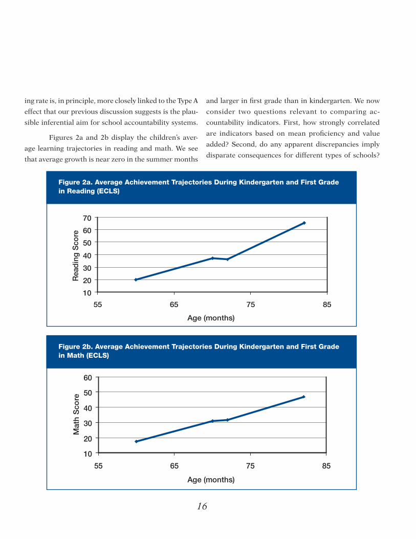
and larger in first grade than in kindergarten. We now
consider two questions relevant to comparing ac-
countability indicators. First, how strongly correlated
are indicators based on mean proficiency and value
added? Second, do any apparent discrepancies imply
disparate consequences for different types of schools?
F2a&b
ing rate is, in principle, more closely linked to the Type A
effect that our previous discussion suggests is the plau-
sible inferential aim for school accountability systems.
Figures 2a and 2b display the children’s aver-
age learning trajectories in reading and math. We see
that average growth is near zero in the summer months
Figure 2a. Average Achievement Trajectories During Kindergarten and First Grade in Reading (ECLS)
10
20
30
40
50
60
70
55 65 75 85
Age (months)
Rea
din
g S
core
Figure 2b. Average Achievement Trajectories During Kindergarten and First Grade in Math (ECLS)
10
20
30
40
50
60
55 65 75 85
Age (months)
Mat
h S
core

17
To answer these questions, I estimated a three-
level hierarchical linear model (Raudenbush & Bryk,
2002) in which each student’s outcome is regarded as
the sum of entry status at kindergarten plus a kinder-
garten growth rate, a summer growth rate, and first year
growth rate plus random error. The two academic-year
growth rates, in turn, varied over children within schools
and over schools. This enabled me to estimate, for each
school and for the sample as a whole, the mean status of
children at each time point and the mean academic-year
learning rates. In this model, status and learning rates are
potentially correlated at the student and the school level.
Correlations between indicators. Suppose now
that school systems were to hold their schools account-
able for kindergarten outcomes. How similar would the
results be using school mean achievement (at spring
kindergarten) versus school value added (mean growth
rate during kindergarten)? The results in Table 1 suggest
that the two approaches would yield fairly similar results.
Thus, we see estimated correlations of r = .77 and r = .71
for reading and math, respectively. These correlations are
corrected for measurement error that arises because, in
any one year, the number of kindergarten students con-
Table 1. Correlations Between Indicators, Kindergarten Through First Grade (ECLS)
Correlation between… Reading Math
Spring kindergarten status and kindergarten value added .77 .71
Spring first-grade status and first-grade value added .55 .06
tributing to the estimates is modest. This news appears
at least somewhat encouraging because its implication
is that schools revealed as effective using mean achieve-
ment have a reasonably high probability of also being
proclaimed effective using the value-added criterion.
The table also presents a comparison between
the two approaches for accountability with respect
to first-grade outcomes. We see that, in this case, the
results are much less encouraging, especially in the
case of math. Specifically, the correlation between
mean achievement in the spring of first grade and value
added (the mean gain during first grade) is r = .55 for
reading and a remarkably small r = .06 for math. A
correlation of .55 implies that a fairly large number
of schools proclaimed effective by a criterion of mean
achievement would not be so proclaimed using value
added—and vice versa. A correlation of .06 implies es-
sentially no association between the results of the two
approaches. This means that knowing that a school
was proclaimed effective on the basis of its spring first
grade mean achievement would tell us nothing about
the average learning rates of children in that school.

18
These discrepant results are open to a variety
of interpretations. One interpretation arose in the
previous section as a potential criticism of the value-
added approach. It could be that schools that are ef-
fective in producing kindergarten gains simply sustain
those gains in first grade without adding to them. This
would explain why schools that appear effective in
kindergarten math according to either criterion ap-
parently have no better growth rates in grade 1 than
do schools that are less effective in kindergarten.
An alternative interpretation is based on selection
bias. Table 2 provides correlations between school mean
entry status and growth rates for reading and for math. I
define entry status as school mean achievement on the fall
kindergarten test. We see nontrivial positive correlations
in both reading and math between entry status and kin-
dergarten growth rates (r = .30 and r = .36, respectively).
To some extent, schools displaying favorable growth rates
during kindergarten may simply be enjoying favorable
selection: Their students entered school ahead and were
primed for more rapid growth. A very different interpre-
tation is that schools serving advantaged students—those
with high entry status—are simply more effective.
The interpretation based on selection bias finds
some support from results in Table 2, which displays
correlations between entry status and growth rates
among students attending the same school. Looking at
reading, we see that, within the same school, students
who started kindergarten ahead tended to grow faster
in reading than did students who started out behind.
This student-level correlation is r = .30, the same as
the correlation at the school level. For math, it is also
clear that entry status and rate of growth are correlated
within schools, r = .27. So apparently, part of the reason
why kindergarten mean proficiency and kindergarten
growth are positively associated is that children who start
school ahead tend to grow faster during kindergarten
even when those students are attending the same school.
Table 2. Correlations Between Entry Status and Growth Rates
School level Reading Math
Correlation between . . .
Entry status and kindergarten growth rate .30 .36
Entry status and first-grade growth rate .21 –.27
Among students within schools
Correlation between . . .
Entry status and kindergarten growth rate .30 .27
Entry status and first-grade growth rate –.25 –.51

19
The evidence in favor of selection bias does not
rule out the possibility that part of the association be-
tween spring kindergarten achievement and kindergarten
growth rates represents underlying school effectiveness
(in the sense of Type A effects as discussed in the pre-
vious section). But it is difficult to quantify this or to
warrant such an interpretation in any confident way.
Turning to the first grade results, we noted that,
in contrast to the kindergarten results, the correlations
between the two indicators—mean proficiency and value
added—were modest or null. Why does this occur in first
grade but not kindergarten? Looking at the first-grade
growth rates at the school and student levels provides
some insight into this puzzle. We see that students who
started school ahead in either reading or math, while
growing more rapidly than other students during kinder-
garten, displayed somewhat smaller growth during first
grade in reading (r = -.25) and in math (r = -.51) (Table
2). This aspect of selection bias may help us understand
why mean proficiency and value added give different
answers in first grade. The negative correlation between
entry status and first-grade growth among students
attending the same school is itself open to several inter-
pretations. It may be that children who started ahead and
gained a lot in kindergarten were unable to grow fast in
first grade because teachers needed to attend more to
children who had not learned so much. But these nega-
tive correlations might also be explained by differences
in the timing of developmental spurts. The children
growing fast in kindergarten might be early bloomers
while children growing fast in first grade might be late
bloomers. This negative correlation between entry status
and growth in first grade might also reflect limitations
of the first-grade achievement test used in the ECLS.
In sum, there is evidence of some concordance
between indicators based on mean proficiency and value
added during kindergarten. But this concordance may
be deceptive, reflecting in part a tendency of children
who start ahead in kindergarten to grow faster in the
absence of school differences in effectiveness. If so, both
the mean proficiency and the value-added indicators
suffer a common selection bias. Alternative interpreta-
tions based on school effects cannot be dismissed, but
neither can they be affirmed based on the kind of data
collected in studies of school accountability. By first
grade, the two kinds of indicators display weak to mod-
est agreement in reading and no agreement in math, a
result that is also open to conflicting interpretations.
Discrepancies between indicators. The previous
section shows that indicators based on mean achieve-
ment and value added produce discrepant results in
first grade, with less discrepant results in kindergarten.
The next logical question is whether identifiable sub-
sets of schools stand to benefit or lose as a result of a
system’s choice of indicator. Given the well-publicized
tendency of high-poverty schools to be proclaimed
failing when mean-proficiency indicators are at play,
it becomes especially interesting to see whether the
adoption of a value-added system would place these
schools in a different light. I define a school’s poverty
level as the fraction of its students who are eligible for
free or reduced lunch. High-poverty schools are those
in which more than 50% of the students are eligible.
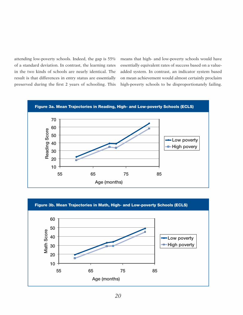
To answer this question, Figures 3a and 3b plot
the expected trajectories of achievement in reading and
math. The results are striking. In math, the average entry
status (fall kindergarten) is substantially lower for stu-
dents attending high-poverty schools than for students
20
attending low-poverty schools. Indeed, the gap is 55%
of a standard deviation. In contrast, the learning rates
in the two kinds of schools are nearly identical. The
result is that differences in entry status are essentially
preserved during the first 2 years of schooling. This
Figure 3a. Mean Trajectories in Reading, High- and Low-poverty Schools (ECLS)
10
20
30
40
50
60
70
55 65 75 85
Age (months)
Rea
din
g S
core
Low povertyHigh povery
Figure 3b. Mean Trajectories in Math, High- and Low-poverty Schools (ECLS)
10
20
30
40
50
60
55 65 75 85
Age (months)
Mat
h S
core
Low povertyHigh poverty
means that high- and low-poverty schools would have
essentially equivalent rates of success based on a value-
added system. In contrast, an indicator system based
on mean achievement would almost certainly proclaim
high-poverty schools to be disproportionately failing.
F3a&b

21
In reading, the basic story is similar with
somewhat different detail. Once again, students in low-
poverty schools have substantially higher entry sta-
tus than do students in low-poverty schools. This gap
remains essentially unchanged during kindergarten but
then widens somewhat during first grade. Once again, an
indicator system based on value added would produce
similar results for high- and low-poverty schools during
kindergarten, while a system based on mean achievement
would disproportionately proclaim high-poverty schools
to be failing. Both systems would proclaim low-poverty
schools to be more effective, on average, than high-pover-
ty schools by the end of first grade, though this tendency
would be much more sharply pronounced for the mean
proficiency indicator than for the value-added indicator.
How shall we interpret the remarkably disparate
impact these two indicators would have on high-poverty
schools? It seems clear that the negative consequences
of a mean achievement indicator system are based al-
most entirely on selection bias. Entry status differences
between high- and low-poverty schools are large whereas
growth rate differences are either nonexistent (in the
case of math) or small (in the case of reading). While
our results cannot affirm that school differences in value-
added validly reflect school differences in effectiveness
(Type A effects, that is), they do cast strong doubt on the
validity and fairness of the mean achievement indicators
based on this national sample of elementary schools.
LATER ELEMENTARY RESULTS
Most of the energy in constructing indicators for
school accountability has focused on grades 2-5. High-
stakes assessment has rarely focused on kindergarten and
only somewhat more often on first grade. Unfortunately,
no nationally representative data sets are currently avail-
able for comparing indicators based on mean achieve-
ment to those based on value added. As a reasonable
substitute, I shall analyze data from two sources: the
Sustaining Effects Study (SES) data (Carter, 1984),
which served as part of the national evaluation of the
Title I program during the early 1980s, and account-
ability data collected on students attending elementary
schools in Washington, DC, between 1998 and 2002
(Bryk et al., 2003). The SES data are old and national
while the Washington, DC, data are new and local. I
view these contrasts as strengths in supporting gen-
eralizability of the results across time and context.
Two questions are again of interest: a) Do the two
approaches (mean proficiency versus value added)
produce different results? b) Do these differences have
disparate impacts on high- and low-poverty schools?
Sustaining Effects Study. The design of the
SES is similar to that of the ECLS in that students
were tested in the fall and spring, again enabling
a decomposition of annual growth in reading and math
into academic and summer components. The differ-
ence is that, whereas the ECLS allows study of trajec-
tories beginning in the fall of kindergarten through
the end of the first grade, the SES begins in the spring
of first grade and ends in the spring of third grade.
Figures 4a and 4b display the average trajectories
of achievement for reading and math based on the SES.
The results parallel those of the ECLS, with small sum-
mer growth in reading, no summer growth in math, and
large academic-year gains in both subjects. Table 3 pro-
vides correlations between mean proficiency and annual
learning rates. The concordance of the results is higher
than in the earlier grades based on the ECLS, especially
in math and especially by grade 3. Specifically, the cor-
relation between mean proficiency and value added in
third grade is r = .78 for reading and r = .91 for math.

22
Figure 4a. Average Achievement Trajectory in Reading, Grades 1-3 (SES)
Figure 4b. Average Achievement Trajectory in Math, Grades 1–3 (SES)
350
400
450
500
550
70 75 80 85 90 95
Age (months)
Rea
din
g S
core
350
400
450
500
550
70 75 80 85 90 95
Age (months)
Mat
h S
core

23
This apparent convergence has several pos-
sible explanations. First, it may be that as students
persist in school, school contributions to learning ac-
cumulate, so that mean differences between schools
come to reflect mean differences in their Type A ef-
fects. An alternative interpretation is that children
who start ahead tend to grow faster regardless of
what school they attend, creating over time an ever
stronger correlation between learning rates and status.
We can probe this issue to some degree by com-
paring correlations between and within schools as in the
case of the ECLS. We do find positive correlations be-
tween school mean status at the outset of the SES (spring
grade 1) and subsequent rates of academic learning, with
r = .35 for reading and r = .36 for math. We find similar
correlations at the student level: students who start out
ahead (that is, in spring of grade 1) grow faster, with
r = .45 in reading and r = .24 in math, than do students
in the same school who start out behind. So to some
extent, there is evidence that school-level convergence in
means and gains reflects a similar process occurring at
the student level, implying perhaps that the school-level
convergence reflects selection bias rather than causa-
tion. However, this interpretation is quite speculative.
The selection and causation components are difficult to
disentangle without a more rigorous study, particularly
Table 3. Correlations Between Indicators, Grades 2–3 (SES)
Correlation between . . . Reading Math
Spring grade 2 status and grade 2 value added .65 .79
Spring grade 3 status and grade 3 value added .78 .91
because what might be viewed as entry status in the SES
is status at spring first grade, which is partly determined
by prior school effects. Recall that this limitation did not
afflict the ECLS results, which included a measure of
achievement at school entry in the fall of kindergarten.
A nuance of the SES is that it did not follow stu-
dents who left the school (outmovers) nor did it collect
data on new students coming into the school (inmov-
ers). This aspect of the SES design may overstate the
convergence of indicators. Such continuity in school
membership will not generally characterize school ac-
countability data collection systems, which will include
data on all inmovers. A more realistic comparison is
available when we turn to the Washington, DC, data.
Washington, DC, accountability data. Bryk et
al. (2003) studied accountability data collected on all
schools and all nonabsent children attending the Wash-
ington, DC, schools between 1998 and 2002. These data
enable useful comparisons between mean proficiency
and value-added indicators during grades 2-5. Unlike
the ECLS and SES data sets, inmovers were followed
over time, allowing the comparison to be broken down
by the time the students entered the study. Table 4 gives
the correlations for those who started in grade 2 in 1998
and continued in through grade 5. The correlations
between mean proficiency and value-added indicators
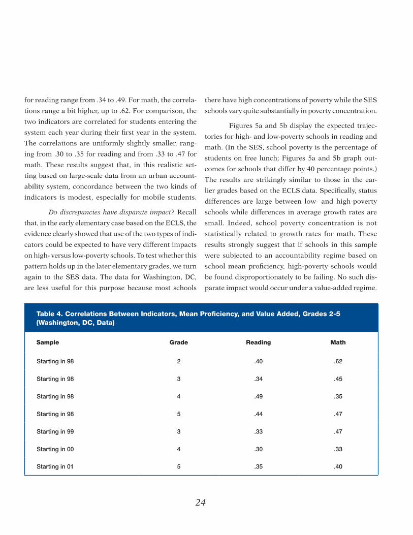
24
for reading range from .34 to .49. For math, the correla-
tions range a bit higher, up to .62. For comparison, the
two indicators are correlated for students entering the
system each year during their first year in the system.
The correlations are uniformly slightly smaller, rang-
ing from .30 to .35 for reading and from .33 to .47 for
math. These results suggest that, in this realistic set-
ting based on large-scale data from an urban account-
ability system, concordance between the two kinds of
indicators is modest, especially for mobile students.
Do discrepancies have disparate impact? Recall
that, in the early elementary case based on the ECLS, the
evidence clearly showed that use of the two types of indi-
cators could be expected to have very different impacts
on high- versus low-poverty schools. To test whether this
pattern holds up in the later elementary grades, we turn
again to the SES data. The data for Washington, DC,
are less useful for this purpose because most schools
Table 4. Correlations Between Indicators, Mean Proficiency, and Value Added, Grades 2-5 (Washington, DC, Data)
Sample Grade Reading Math
Starting in 98 2 .40 .62
Starting in 98 3 .34 .45
Starting in 98 4 .49 .35
Starting in 98 5 .44 .47
Starting in 99 3 .33 .47
Starting in 00 4 .30 .33
Starting in 01 5 .35 .40
there have high concentrations of poverty while the SES
schools vary quite substantially in poverty concentration.
Figures 5a and 5b display the expected trajec-
tories for high- and low-poverty schools in reading and
math. (In the SES, school poverty is the percentage of
students on free lunch; Figures 5a and 5b graph out-
comes for schools that differ by 40 percentage points.)
The results are strikingly similar to those in the ear-
lier grades based on the ECLS data. Specifically, status
differences are large between low- and high-poverty
schools while differences in average growth rates are
small. Indeed, school poverty concentration is not
statistically related to growth rates for math. These
results strongly suggest that if schools in this sample
were subjected to an accountability regime based on
school mean proficiency, high-poverty schools would
be found disproportionately to be failing. No such dis-
parate impact would occur under a value-added regime.

25
Figure 5b. Average Trajectories in Math, Grades 1–3, High- and Low-poverty Schools (SES)
350
400
450
500
550
70 75 80 85 90 95
Age (months)
Mat
h S
core
Low povertyHigh poverty
Figure 5a. Average Trajectories in Reading, Grades 1–3, High- and Low-poverty Schools (SES)
350
400
450
500
550
70 75 80 85 90 95
Age (months)
Rea
din
g S
core
Low povertyHigh Poverty

26
HIGH SCHOOL RESULTS
The National Educational Longitudinal Study of
1988 (NELS:88) provides an extremely useful data set for
the purpose of studying indicators that might be collected
at the high school level. I use the High-school Effective-
ness Supplement of the NELS:88, which represents large
metropolitan areas in the United States. Students were
sampled in 1988 when they were in grade 8. We have in-
formation on their achievement in science and in math in
grade 8 before they entered high school. They were retest-
ed in grades 10 and 12, making it possible to estimate, for
each high school, mean status at grade 8, mean growth
in grades 9–10 and 11–12, and mean status at the end of
grades 10 and 12. Once again we ask whether the indica-
tors based on mean proficiency and value added agree
and, to the extent they do not, whether the differences
have disparate impact on high- and low-poverty schools.
Do the indicators agree? Agreement is com-
paratively high in the case of science and somewhat
more modest in the case of math. To see this, let us
compare a school’s mean proficiency at grade 10 to the
alternative value-added indicator: the school average
growth rate during grades 9 and 10. We find r = .78
in science and r = .59 in math for these two indica-
tors (Table 5a). In part, however, this degree of con-
vergence appears to represent a process of selection.
The correlations between school mean eighth-grade
status and school mean learning rate in grades 9–10
are r = .67 for science and r = .46 for math (Table 5b).
Table 5a. Correlation Between School Mean Proficiency, Grade 10, and Value Added, Grades 9–10 (NELS:88)
Science .78
Math .59
Table 5b. Correlation Between School Mean Proficiency, Grade 8, and Value Added, Grades 9–10 (NELS:88)
Science .67
Math .46
Do discrepancies have disparate impact on high-
and low-poverty schools? Figures 6a and 6b plot the
expected achievement trajectories in science and math,
respectively, for low- and high-poverty schools. (In the
NELS:88, school poverty is the percentage of students
eligible for free lunch. Figure 6 graphs outcomes for
schools that differ by 40 percentage points.) Note the
substantial gap in mean achievement between the two
kinds of schools in the eighth-grade achievement of
their students, showing a strong selection bias. Growth
rates during high school are significantly flatter as well
in high-poverty schools. However, 10th- and 12th-grade
achievement mean differences are more affected by the
initial status differences than by the growth differences.
As a result, we can conclude that an accountability sys-
tem based on mean proficiency would find many more
high-poverty schools failing than would an accountability
system based on value added. The tendency of mean pro-
ficiency to disproportionately target high-poverty schools
as failing appears to result primarily from selection bias.

27
Figure 6b. Average Achievement Trajectories in Math, Grades 8-12 (NELS:88)
Figure 6a. Average Achievement Trajectories in Science, Grades 8-12 (NELS:88)
15
20
25
30
8 10 12
Grade
Sci
ence
Sco
re
Low povertyHigh poverty
30
40
45
35
50
55
60
8 10 12
Grade
Mat
h S
core
Low povertyHigh poverty

28
In sum, looking across the elementary and
high schools years, we find remarkable similarities in
how indicators based on mean proficiency compare
to those based on value added. In general, the degree
of agreement between the indicators is modest, with
correlations in the range of .35 to .60 most typical.
These results suggest that if both systems were used,
the results for individual schools would certainly be
correlated, but that there would be many discrepant
cases. That is, in many cases, schools viewed as thriving
under a mean-proficiency regime would not be found
to thrive under a value-added regime, and vice versa.
Moreover, these differences are systematic in
having disparate impact as a function of schools’ poverty
status. Specifically, at every level of schooling considered
here, high-poverty schools would fare much worse under a
mean proficiency regime than under a value-added regime.
Given that the two approaches have different
consequences for different kinds of schools, many would
argue that value-added indicators are fairer (Sanders et
al., 1997; Bryk, Thum, Easton, & Luppescu, 1998). Not-
withstanding the inferential problems associated with
the value-added approach, a case can certainly be made
to opt for it. Yet while considering the potential biases
of the two approaches, we have not considered their
statistical precision. The value-added approach, in par-
ticular, would be of little use if its virtues are purchased
at the cost of unreliability. We now turn to that issue.

29
CAN WE MEASURE SCHOOL QUALITY AND SCHOOL IMPROVEMENT WITH ADEQUATE RELIABILITY?
ean scores tend to be quite stable when sample
sizes are even modestly large, say in the neighborhood
of 30–50 per school (Raudenbush & Bryk, 2002, chap.
5; see also Raudenbush & Sampson, 1999). Estimates
based on gain scores may be more imprecise. Indeed, a
key motivation for the invention of complex modeling
schemes for value-added analysis is that simple unad-
justed gain scores, even when aggregated to the school
level, may be statistically unstable. Given that many will
tend to prefer value-added indicators for all the reasons
cited in the previous section, it becomes particularly im-
portant to assess the precision of the resulting estimates.
RELIABLE COMPARISONS
At the most practical level, the question is
whether value-added estimates of school quality and
school improvement can support reliable comparisons
between schools given the data routinely collected in an
M accountability system. To answer this question, Bryk et
al. (2003) analyzed data collected on 49,993 students
flowing through 102 public elementary schools in Wash-
ington, DC, from 1998 to 2002. The structure of the data
are displayed in Table 6. Students in Cohort 5 started
first grade in 1998 and provided test scores in grades 1-5
until 2002 (unless those students moved out of Washing-
ton, DC, or were absent at the time of a test). All other
cohorts provided data of shorter duration. For example,
each member of Cohort 4 started in grade 1 in 1999
and potentially produced four test scores—from grade
1 to grade 4. All inmovers—those who began attending
Washington, DC, schools during this period—were fol-
lowed as well. All available data were used in the analysis
based on a rather complex statistical model that views
the repeated measures for each student as cross-classi-
fied by students and schools (Raudenbush & Bryk, 2002,
chap. 12). This approach efficiently uses all available data
and is comparatively robust in the face of missing data.
Table 6. Structure of Washington, DC, Data
Year of testing
Grade 1998 1999 2000 2001 2002
1 C5 C4 C3 C2 (C1)
2 C6 C5 C4 C3 C2
3 C7 C6 C5 C4 C3
4 C8 C7 C6 C5 C4
5 C9 C8 C7 C6 C5
Note. Data reflects a total of 49,993 students flowing through 102 schools over a 5 year period (Bryk et al., 2003). C = cohort

30
Sample sizes for each data pattern are displayed
in Table 7. The table reveals the complexity of the data
commonly yielded in school accountability systems. To
understand Table 7, let’s begin by looking at the data for
Cohort 5.0, those who began first grade in 1998, here
5,715 students. By second grade (1999), a number of
the original students had left the system or were absent
at the time of the test, so only 3,881 were tested. This
number diminished each year, so that by grade 5 (2002),
only 2,864 of the original students remained available
for testing. Similar patterns occur for other cohorts.
The data also include inmovers. For example, consider
Table 7. Analytic Sample in Cohort Order in Reading (Washington, DC, Data)
Year of testing
First year First grade Cohort 1998 1999 2000 2001 2002
2001 1 2.0 4,935 3,575
2000 1 3.0 5,306 4,328 3,345
2001 2 3.1 854 498
1999 1 4.0 4,935 3,692 3,571 2,906
2000 2 4.1 1,242 915 621
2001 3 4.2 584 304
1998 1 5.0 5,715 3,881 3,855 3,699 2,864
1999 2 5.1 1,302 814 750 526
2000 3 5.2 916 642 337
2001 4 5.3 420 203
1998 2 6.0 4,998 3,480 3,296 3,102
1999 3 6.1 1,319 950 828
2000 4 6.2 838 543
2001 5 6.3 376
1998 3 7.0 4,980 3,446 3,254
1999 4 7.1 1,066 656
2000 5 7.2 898
1998 4 8.0 4,134 2,751
1999 5 8.1 876
1998 5 9.0 3,591

31
Cohort 5.1, which includes students who first appeared
in the system in grade 2 (1999). There were 1,302 of these
inmovers, but by grade 5 (2002), only 526 remained. The
complexity of these data, with outmovers, inmovers, and
absentees, poses serious challenges to statistical analysis,
Figure 7a. School-specific Estimates of Value Added for the Initial Year
- -- - - -
-
- - - --
-- - - - -
- - -- - - -
- - - - - -- - - -
- --
- - - - --
--
- - - - - - - - - - - -- - -
- - -- - - - - - -
- - - -- -
- - --
- -- - - - -
-
- - -- - -
--
- - -
- -- - -
-
-
- - - - --- - - - - - - - - -
- -- - - - - - - - - - - -
- - - - - -- -
-- - - - - - - - - - - -
- - -- - -
- - - - - --
- - - -- -
- --
-- - - - - - -
-
- -- - - -
--
- - -
-
--
-
Initial Value AddedStanford 9 Reading Test
Schools
Initi
al V
alue
Ad
ded
-10
100
explaining in part why statistical methods for value-
added analysis have become complex (Wainer, 2004).
Figures 7a, 7b, and 7c show how Bryk et al. (2003)
recommend displaying results. Schools are ranked in
terms of their value added in 1999 (Figure 7a), aver-
Figure 7b. School-specific Estimates of Value Added Averaged Over 5 Years
--
- - - -- - - - - - - - - - - - - - - - - - - - - - - - - -
- - - - - - - - - - - - - - - - - - - - - - - - - - - - - - - - - - - - - - - - - - - - - - - - - - - - - -- - - - - -
-
- - - -- - -
-- - - -
- - - - - - - - - - - - - - - - - - - - - - - - - - - - - - - - - - - - - - - - - - - - - - - - - - - - - - - - - - - - - - - - - - - - - - - - - - -- - - - -
- - - - - - -- - - - -
- - -
-
-
Ave
rag
e Va
lue
Ad
ded
-10
100
Average Value AddedStanford 9 Reading Test
Schools
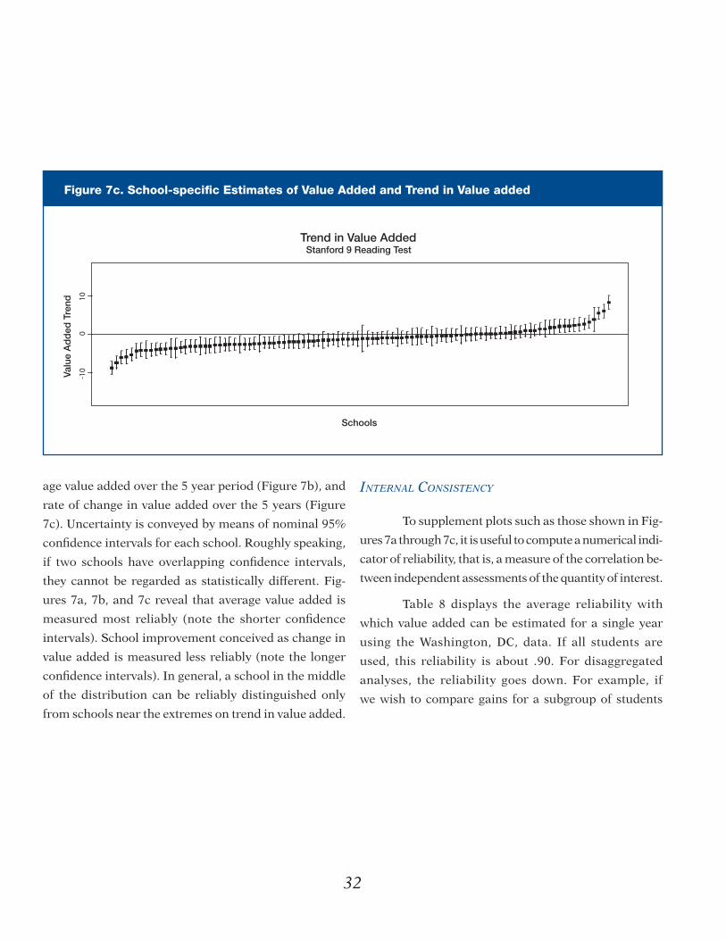
32
Figure 7c. School-specific Estimates of Value Added and Trend in Value added
--
- - - - - - - - - - - -- - - - - - - - - - - - - - - - - - - - - - - - - - - - - - - - - - - - -
-- - - - - - - - - - - - - - - - - - - - - - - - - - - - - - - - - - - - - - - - - - - - - - -
-
-
--
- - -- - - - - - -
- - - - - - - - - - - - - - - - - - - - - - - - - - - - - - - - - - - - - - --
- - - - - -- - - - - - - - - - - - - - - - - - - - - - - - - - - - - - - - - - - - - - - -
- -
-
-
-
Valu
e A
dd
ed T
rend
-10
100
Trend in Value AddedStanford 9 Reading Test
Schools
age value added over the 5 year period (Figure 7b), and
rate of change in value added over the 5 years (Figure
7c). Uncertainty is conveyed by means of nominal 95%
confidence intervals for each school. Roughly speaking,
if two schools have overlapping confidence intervals,
they cannot be regarded as statistically different. Fig-
ures 7a, 7b, and 7c reveal that average value added is
measured most reliably (note the shorter confidence
intervals). School improvement conceived as change in
value added is measured less reliably (note the longer
confidence intervals). In general, a school in the middle
of the distribution can be reliably distinguished only
from schools near the extremes on trend in value added.
INTERNAL CONSISTENCY
To supplement plots such as those shown in Fig-
ures 7a through 7c, it is useful to compute a numerical indi-
cator of reliability, that is, a measure of the correlation be-
tween independent assessments of the quantity of interest.
Table 8 displays the average reliability with
which value added can be estimated for a single year
using the Washington, DC, data. If all students are
used, this reliability is about .90. For disaggregated
analyses, the reliability goes down. For example, if
we wish to compare gains for a subgroup of students

33
Table 8. Reliability of Single-year Value-added Estimate in Reading (Washington, DC, Data)
Percentage of students used Reliability
100 .90
50 .83
33 .76
25 .70
20 .66
based on ethnicity, the reliability would be just .76 if
that subgroup constituted 33% of a school's sample.
Table 9 provides a similar display, but for the
reliability of the average value added over 3, 4, or 5 years.
Not surprisingly, these reliabilities are much higher
than the reliabilities for a single year—near 1.0 unless
the percentage of students contributing is quite small.
Table 10 provides reliabilities for measuring
school improvement as a function of the number of years
of data collection and the percentage of students to be
compared. These results are more sobering. Even when
the data span 5 years and all students are used, the reli-
ability is .86—respectable, but still conveying some degree
of uncertainty about a school’s rate of increase. Compari-
sons among subgroups in terms of school improvement
do not appear to be supported unless the subgroup con-
stitutes half the school sample and unless 5 years of data
are collected. Even then, reliability is a fairly modest .76.
Lack of reliability will tend to exacerbate a
problem discussed in detail earlier: the degree of con-
vergence between indicators based on mean proficiency
and value added. The correlations in the previous tables
were corrected for measurement error. In practice,
correlations between school-level indicators will tend
to be even smaller than those reported in the tables.

34
Table 9. Reliability of Average Value Added in Reading (Washington, DC, Data)
Percentage of students used 3 years 4 years 5 years
100 .96 .98 .99
50 .92 .96 .97
33 .89 .95 .96
25 .85 .93 .95
20 .82 .92 .94
Table 10. Reliability of Improvement (Rate of Change of Value Added) as Function of Years of Data Collection in Reading (Washington, DC, Data)
Percentage of students used 3 years 4 years 5 years
100 .52 .79 .86
50 .36 .66 .76
33 .27 .56 .68
25 .22 .49 .61
20 .18 .43 .56
Table 11. Correlation Between Change in Mean Proficiency Indicators and Change in Value-added Data (Washington, DC, Data)
Reading .07
Math .15
Table 11 gives correlations from Bryk et al.
(2003) between change in school-average proficiency
and change in value added based on the Washington,
DC, data. These results show essentially no associa-
tion between the two. Clearly, the two approaches give
very different impressions about school improvement.

35
WHAT ARE THE IMPLICATIONS FOR COLLECTING, REPORTING, AND USING SCHOOL ACCOUNTABILITY DATA?
he logical analysis and empirical evidence emerg-
ing from this inquiry lead to the following conclusions:
1. High-stakes decisions based on school-mean pro-
ficiency are scientifically indefensible. We cannot
regard differences in school mean proficiency as
reflecting differences in school effectiveness. Instead,
as data from the ECLS showed, school differences in
mean proficiency during the early grades primarily
reflected school differences in the cognitive status of
the children those schools served at the time those
children entered school in the fall of kindergarten.
And as data from the NELS:88 showed, school mean
differences among high schools for grades 10 and 12
strongly reflected the mean differences between the
students those schools served when those students
were in grade 8, before those students entered high
school. To reward schools for high mean achievement
is tantamount to rewarding those schools for serving
students who were doing well prior to school entry.
2. The unjustifiable use of school-mean proficiency for
high-stakes decisions will disparately affect schools
serving poor children:
• Early in elementary school (grades k-1), high-
and low-poverty schools differed substantially in
mean proficiency, but these differences strongly
reflected differences among the students those
schools served at entry to kindergarten. Perhaps
surprisingly, average rates of academic learning in
high- and low-poverty schools were quite similar
in mathematics and slightly different in reading.
This means that mean differences in proficiency
between high- and low-poverty schools at the
end of first grade primarily reflected mean differ-
ences observable during the fall of kindergarten.
It follows that an accountability system using
T low-school mean proficiency to label schools as
failing would have disproportionately identified
high-poverty schools as failing. In contrast, a system
using value-added indicators (school mean rates
of learning) would not have produced this result.
• During the middle elementary grades (grades 2 and
3), the story is similar. School poverty concentration
was unrelated to growth rates in math. Thus, mean
proficiency differences at the end of each grade in
math reflected mean differences at the beginning
of the school year. In reading, low-poverty schools
displayed less growth, on average, than did high-
poverty schools, but these differences were small
compared to the differences at the beginning of
the school year. Hence, end-of-year differences
in mean proficiency in reading between low- and
high-poverty schools were more influenced by
differences in entry status than by differences
in growth rates. Again, an accountability system
proclaiming schools with low mean proficiency to
be failing would have disproportionately and un-
justifiably found high-poverty schools to be failing.
• At the high-school level, a similar picture emerg-
es. Students entered high-poverty high schools
with considerably lower proficiency in math
and science than did students entering low-pov-
erty schools. Those differences widened as high-
poverty schools displayed lower growth rates than
did low-poverty schools. Nonetheless, mean differ-
ences in proficiency between high- and low-poverty
schools in grades 10 and 12 reflected school-mean
differences in grade 8 more than school mean
differences in growth rates. Once again, basing
high-stakes decisions on school mean proficiency
would have unfairly affected high-poverty schools.
Related Documents