School of Economics UNSW, Sydney 2052 Australia http://www.economics.unsw.edu.au ISSN 1323-8949 ISBN 978 0 7334 2550 9 Household Wealth Accumulation and Portfolio Choices in Korea Sang-Wook (Stanley) Cho School of Economics Discussion Paper: 2007/26 The views expressed in this paper are those of the authors and do not necessarily reflect those of the School of Economic at UNSW.

Welcome message from author
This document is posted to help you gain knowledge. Please leave a comment to let me know what you think about it! Share it to your friends and learn new things together.
Transcript

School of Economics UNSW, Sydney 2052
Australia
http://www.economics.unsw.edu.au
ISSN 1323-8949
ISBN 978 0 7334 2550 9
Household Wealth Accumulation and Portfolio Choices in Korea
Sang-Wook (Stanley) Cho
School of Economics Discussion Paper: 2007/26
The views expressed in this paper are those of the authors and do not necessarily reflect those of the School of Economic at UNSW.

Household Wealth Accumulation and Portfolio Choices in Korea
Sang-Wook (Stanley) Cho ∗University of Minnesota
October 2005
Job Market Paper
Abstract
This paper constructs a quantitative lifecycle model with uninsurable labor income and
aggregate housing return risk to assess how Korean households make saving and portfolio
allocation decisions. The model incorporates the special roles housing plays in the portfolio
of households: collateral, a source of service flows, as well as a source of potential capital
gains or losses. In the model, a household first makes the decision whether to rent or to buy
a house and then chooses the housing value. The model adds to existing models of wealth
accumulation some unique institutional features present in Korea, namely the rental system
(‘chonsae’) and the lack of a mortgage system. When the model is calibrated to match
the Korean economy, several key features of the data are better able to be reproduced. The
paper also analyzes the role of institutional features by comparing several alternative housing
market arrangements and the introduction of a pay-as-you-go social security system to assess
their impact on wealth accumulation, portfolio choices, and the pattern of homeownership.
I find that expanding the mortgage system significantly increases the homeownership ratio,
while alternative rental arrangements have mixed effects on the homeownership ratio. All
of the alternative market arrangements raise the fraction of household wealth invested into
housing assets. I also find that the introduction of social security system will lower the overall
savings in Korea by approximately 10% and lower the homeownership ratio by 6 percentage
points.
JEL classification : D91, E21, H31, R21
Keywords : Lifecycle Model, Consumption, Wealth, Housing, Korea∗I am deeply grateful to my advisors, Larry Jones and Mariacristina De Nardi, for their guidance and help.
I also thank V.V. Chari, Javier Fernandez-Blanco, Nicolas Figueroa, Annie Fang Yang, and participants at the
Growth and Development Seminar for their valuable comments and suggestions. All remaining errors are my
own. I can be reached at 271 19th Avenue S, Department of Economics, University of Minnesota, Minneapolis,
MN 55455, U.S.A., Email: [email protected].

1 Introduction
In this paper, I examine the Korean household’s wealth accumulation and asset portfolio choices
over the life cycle. Empirical studies about household portfolios have been undertaken in some
developed countries, but little attention has been paid to developing countries mainly due to
the lack of quality data. I use the recent Korea Labor Income Panel Study (KLIPS) to examine
how average Korean households accumulate their wealth over the life cycle. I then make a
cross-country reference in order to highlight the differences in the profile of various assets in the
aggregate as well as over the age-groups. This enables me to pay close attention to the points
that are specific to Korea.
Housing is the most important form of wealth in Korea. According to the KLIPS data, while
approximately 60% of households are homeowners, housing assets make up close to 50% of total
assets held by all households. The share of financial assets, on the other hand, is around 25%.
This is a significant departure from the United States, where the homeownership ratio is around
68% and the shares of housing and financial assets are approximately 30% and 37%, respectively.
Thus, despite a lower homeownership ratio in Korea, for those who are homeowners, housing
becomes the most predominant source of wealth. This also indicates that the decision to purchase
a house has important implications for the portfolio composition of a Korean household over the
life cycle, as housing not only provides a flow of service for consumption but also can be used
as a source of investment.
Unique to the Korean economy is the existence of a ‘chonsae’ system, a rental market system
in which a tenant pays a deposit upfront (usually 40-80% of the property value) with no addi-
tional periodic rent payments, and receives the nominal value of the deposit from the landlord
upon maturation. Given this structure of the chonsae system, renters in Korea have a proportion
of their assets indirectly tied up to housing with zero nominal returns. This contrasts sharply
with the situation in the United States, where renters do not own any assets related to housing
and therefore are able to diversify their financial portfolio. Another unique aspect is the lack
of an affordable mortgage system, which reflects the under-developed nature of the financial
sector in Korea. For instance, Lam (2002) reports the average mortgage to GDP ratio in Ko-
rea between 1996 and 2000 to be around 11%, whereas the corresponding figure in the United
States was approximately 55%. Also, the average loan-to-value ratio1 during the same period
was 28% in Korea, as opposed to around 80% in the United States. A full-scale government-
endorsed mortgage system was only introduced in 2004, prior to which such a system was almost
non-existent.1Loan-to-value (LTV) ratio is defined as the ratio of the fair market value of an asset to the value of the loan
that will finance the purchase.
1

I set up a partial equilibrium lifecycle model allowing for these specific housing features in
Korea and I calibrate it to match wealth accumulation and portfolio choice over the life cycle. In
the model, housing plays multiple roles in the economy as not only a source of direct consumption
but also as an investment with potential for capital gains and collateral. The results from the
calibrated model can quantitatively explain some empirical findings on the profile of wealth and
homeownership in the aggregate as well as over the life cycle.
In addition, I assess the roles played by the institutional features of the mortgage market
and the rental market arrangement, and ask how much they can individually and jointly account
for the observed pattern of the wealth accumulation and portfolio composition in Korea. For
the mortgage market, an expansion of the current mortgage system is represented by a higher
loan-to-value ratio. Expanding the current mortgage system lowers the overall level of wealth
accumulation in the economy, while increasing the homeownership ratio and the fraction of
wealth invested into housing assets. Wider availability of mortgage loans weakens the saving
motives since households, especially younger ones, save primarily to purchase a house. However,
as it becomes easier for households to purchase a house, the fraction of wealth invested into
housing and the overall homeownership increase. For reasonable parameter values, I find that
increasing the loan-to-value ratio to 70% will cause a 3% decrease in the aggregate net worth, a
11 percentage point increase in the homeownership ratio, and a 14 percentage point increase in
the fraction of wealth invested into housing asset.
Next, the rental arrangement in the benchmark model is altered such that in lieu of a lump-
sum deposit, households pay periodic rental payment which is assumed to be a fraction of the
house value. The annual rental cost ranges from 2% to 6% of the value of the house. For lower
rental cost, this results in a decrease in the overall level of wealth accumulation as well as a
lower homeownership ratio, since renting becomes a cheaper alternative to homeownership and
lowers the need for savings geared towards housing purchase. For the annual rental cost of 2%,
the aggregate net worth and the homeownership ratio decline by 9% and 7 percentage points,
respectively. In addition, the fraction of wealth in housing assets falls by 4 percentage points.
On the other hand, for higher rental cost parameter values, the overall net worth, the fraction of
wealth invested into housing assets, and the homeownership ratio increase. For the annual rental
cost of 6%, the overall net worth increases by 3%, while the fraction of wealth held in housing
assets and the overall homeownership ratio increase by 5 and 7 percentage points, respectively.
When the mortgage system and the rental arrangement are jointly modified, the overall level
of wealth accumulation declines by 2% to 10%, depending on the rental cost. On the other
hand, the experiment results in an increase in the homeownership ratio by 4 to 15 percentage
points, and an increase in the share of wealth held in housing assets by 10 to 17 percentage
2

points. The decrease in the overall net worth is due to wider availability of mortgage loans or
cheaper rental cost. Looking at different age groups, expanding the mortgage system mainly
targets younger households, whereas different rental arrangement have relatively larger impact
on older households as they decide whether to remain homeowners or become renters.
Finally, I use the model to analyze the quantitative effects of introducing a pay-as-you-go
(PAYG) social security system upon the pattern of wealth accumulation and portfolio choice over
the life cycle. The social security experiment shows that the overall level of wealth also declines,
since the availability of social security benefits after retirement weakens the saving motives of
households during their working ages. Lowering the level of wealth accumulation has implications
for the households’ housing purchase, as less households can afford to purchase owner-occupied
housing. In contrast to expanding the mortgage system, the social security system lowers the
overall homeownership ratio as well. The impact of social security on the composition of wealth
is weak, since the effects of lower wealth accumulation and lower homeownership offset each
other. The quantitative effect of a PAYG social security system is a 10% reduction in the
aggregate net worth and a 6 percentage point decline in the homeownership ratio.
This paper builds on the emerging literature that document household portfolio allocation2.
With a few papers allowing for housing in models of portfolio choice, the role of housing wealth
has received greater attention due to its unique role: people can borrow against housing; housing
is indivisible and relatively illiquid (buying and selling entail significant liquidation costs); and
housing not only provides a flow of real benefits to the owner as a consumption good, but also,
acts as an investment good that provides potential for capital gains or losses. Grossman and
Laroque (1990), using an infinite horizon model, are the first to analyze housing in the portfolio
allocation in the presence of adjustment costs. Dıaz and Luengo-Prado (2002) and Gruber and
Martin (2003) also use a standard infinite horizon model to study the role of durable goods and
collateral credit in accounting for wealth inequality and the level of precautionary savings in
the United States. Cocco (2004) specifies the housing price risk to study the asset allocation
decision in the presence of housing. Some papers explicitly include housing in the context of a
general equilibrium lifecycle framework. For example, Chen (2004) investigates the implications
of privatizing social security system, while Yang (2005) matches the profile of housing in the
United States. Chambers, Garriga and Schlagenhauf (2004) use a similar framework to examine
the recent changes in the US homeownership ratio. Other important works include, among many
others, Fernandez-Villaverde and Krueger (2001), Flavin and Yamashita (2002), and Campbell
and Cocco (2003). Additionally, an alternative to the housing market is that people can rent
instead of purchasing a house. In the case of renting, renters receive a similar flow of services,2A comprehensive review of the literature is provided by McCarthy (2004).
3
although somewhat less than from their own house, and are not subject to capital gains or losses.
Platania and Schlagenhauf (2000), Ortalo-Magne and Rady (2003), Hu (2003), Yao and Zhang
(2003), Miles, Cerny and Schmidt (2004), Li and Yao (2005) all explicitly incorporate the rental
versus homeownership decision into their models.
In general, models of housing have made predictions closer to what have been observed empir-
ically in areas such as wealth distribution, household portfolio allocations, and tenure decisions;
however, these models have been calibrated mostly to the United States. It would be interesting
to evaluate the predictions of these models on other economies while incorporating their unique
features. This will indirectly help to examine the role of these features in accounting for the
differences in wealth accumulation and portfolio choice across countries. This paper makes a
first attempt to fill this void and extends beyond the literature by offering distinct contributions
in both empirical and theoretical aspects. First, the paper conducts an empirical study of wealth
in Korean households from the KLIPS data and points out some stylized facts in the average
wealth portfolio as well as the cross-section profile of various assets and homeownership ratios by
age groups. It highlights the similarities and differences in the pattern of wealth accumulation
and portfolio choice with those shown in the United States and other countries. Theoretically,
the model framework of this paper is closest in spirit to Miles, Cerny and Schmidt (2004). They
also set up a calibrated model in the context of uninsurable labor income and uncertainties in
housing price to simulate the housing and portfolio choice of Japanese households and study the
impact of changes in the social security regimes and demography. However, this paper explores
several other distinct aspects. First, my model set-up explicitly incorporates the chonsae system
in the Korean housing market, which is not modelled in Miles, Cerny and Schmidt (2004). Sec-
ond, the paper looks at the mortgage institutions in Korea and explores the joint implications
of the specific rental choices and mortgage institutions faced by Korean households. The model
is then calibrated to the Korean economy, providing the groundwork for various policy analyses.
The paper then highlights the role of institutional factors by altering the market institutions
individually and jointly, and examine the impact on the profile of wealth, wealth composition,
and homeownership.
The rest of this paper is organized as follows. Section 2 presents the empirical findings
and stylized facts from the analysis of the KLIPS data and documents some features of wealth
accumulation and portfolio changes for average Korean households. Section 3 describes the cal-
ibrated lifecycle model framework. Section 4 outlines the calibration and the parametrization of
the model. In Section 5, I present the results from the benchmark simulation, and quantitatively
assess the roles played by the housing market institutions in Korea as well as some implications
of introducing a pay-as-you-go (PAYG) social security system. Section 6 conducts a sensitivity
4

analysis, and brief concluding remarks are provided in Section 7. The appendix presents the
model set up for an alternative rental arrangement, algorithms for the computation, and the
figures from the sensitivity analysis.
2 Data and Empirical Evidence
2.1 Average Wealth Portfolio
In this study, I use the Korean Labor Income Panel Study (KLIPS) from 1998 to 2002. It is a
socio-demographic panel study which includes data about household income and wealth. In the
wealth category, the KLIPS survey asks households about various types of assets and liabilities.
I group assets into primary housing (“House”), financial assets, and other non-financial assets
excluding owner-occupied housing such as secondary home, land, and rental real estate (“Other
non-financial”). Within the financial assets category, I closely examine different financial assets,
such as rent deposit, time deposits (checking and savings account), stocks and bonds, and life
insurance. A rent deposit, or ‘chonsae’ deposit, is a lump-sum deposit in lieu of periodic rental
payments that is unique to Korea. Since renters pay an upfront deposit at the beginning of the
contract and receive the exact nominal amount back at the end of the contract, a chonsae is
considered a financial instrument with a zero nominal interest rate3. I also look at outstanding
financial liabilities. Net worth is defined as the difference between total assets and total financial
liabilities. Table 1 below summarizes the wealth holdings of the average household for each asset
type from the 2001-2002 KLIPS data. For reference, the table also shows the average wealth
holdings in the United States compiled by Kennickell (2003), which uses the 1995 Survey of
Consumer Finances.
Table 1. Summary Statistics of Average Wealth - Korea vs. United States
Korea United States
Total asset(normalized by average income) 5.247 5.560- House 2.580 1.670- Financial asset 1.315 2.041
¦ Rent deposit 0.613 -¦ Deposits 0.450 0.399¦ Stock & Bond 0.074 0.852¦ Insurance 0.089 0.147¦ Others 0.089 0.643
- Other non-financial 1.352 1.849Total liabilities 0.816 0.813Net Worth 4.431 4.747
3The survey also asks landlords whether or not they have received the chonsae deposit. Since this is considered
part of the financial liabilities, there is no double counting of financial assets in the aggregate.
5
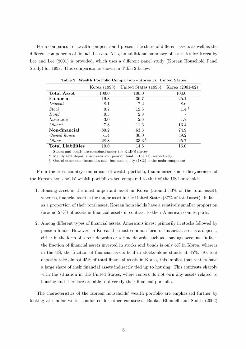
For a comparison of wealth composition, I present the share of different assets as well as the
different components of financial assets. Also, an additional summary of statistics for Korea by
Lee and Lee (2001) is provided, which uses a different panel study (Korean Household Panel
Study) for 1998. This comparison is shown in Table 2 below.
Table 2. Wealth Portfolio Comparison - Korea vs. United States
Korea (1998) United States (1995) Korea (2001-02)Total Asset 100.0 100.0 100.0Financial 19.8 36.7 25.1Deposit 8.1 7.2 8.6Stock 0.7 12.5 1.4 †Bond 0.3 2.8 -Insurance 3.0 2.6 1.7Other ‡ 7.8 11.6 13.4Non-financial 80.2 63.3 74.9Owned house 51.4 30.0 49.2Other 28.8 33.3 § 25.7Total Liabilities 10.0 14.6 16.0† Stocks and bonds are combined under the KLIPS survey.‡ Mainly rent deposits in Korea and pension fund in the US, respectively.§ Out of other non-financial assets, business equity (18%) is the main component.
From the cross-country comparison of wealth portfolio, I summarize some idiosyncracies of
the Korean households’ wealth portfolio when compared to that of the US households.
1. Housing asset is the most important asset in Korea (around 50% of the total asset);
whereas, financial asset is the major asset in the United States (37% of total asset). In fact,
as a proportion of their total asset, Korean households have a relatively smaller proportion
(around 25%) of assets in financial assets in contrast to their American counterparts.
2. Among different types of financial assets, Americans invest primarily in stocks followed by
pension funds. However, in Korea, the most common form of financial asset is a deposit,
either in the form of a rent deposits or a time deposit, such as a savings account. In fact,
the fraction of financial assets invested in stocks and bonds is only 6% in Korea, whereas
in the US, the fraction of financial assets held in stocks alone stands at 35%. As rent
deposits take almost 45% of total financial assets in Korea, this implies that renters have
a large share of their financial assets indirectly tied up to housing. This contrasts sharply
with the situation in the United States, where renters do not own any assets related to
housing and therefore are able to diversify their financial portfolio.
The characteristics of the Korean households’ wealth portfolio are emphasized further by
looking at similar works conducted for other countries. Banks, Blundell and Smith (2002)
6

document the wealth portfolio in the United Kingdom using the British Household Panel Survey
(BHPS), and reports that an average UK household holds 60%4 of total household wealth in
home equity. As for types of financial assets, the BHPS reports a 35% share for stocks and
mutual funds. Iwaisako (2003) studies household portfolios in Japan and shows that financial
assets comprise 31% of the total asset. The rest is invested into housing or other real estate
assets. Looking into the shares of different types of financial assets, time deposits make up 46%
of total financial assets followed by life insurance at 41%. The share of stocks and bonds is
only around 8% of total financial assets. The cases of the United Kingdom and Japan indicate
some similarities in the composition of the wealth portfolio in Korean, Japanese, and British
households in contrast to American households. Excluding the United States, not only is housing
(or home equity) the most important investment, but also the portfolio composition of the
financial assets is more risk-averse, with only a small fraction invested in risky assets such as
stocks.
One issue is how well the household survey of wealth matches the aggregate measures. On
top of the usual misreporting problem, the KLIPS data does not over-sample the wealthy, and,
thus, gross wealth estimated from the survey is likely to under-represent the aggregate wealth of
the economy. Regarding the composition of wealth, since the wealthy tend to hold more of their
wealth in financial assets other than housing, the relative share of financial assets is expected to
be higher in the aggregate economy than in the KLIPS data. Further study is needed to bridge
the gap between the two different data sources.
2.2 Wealth Portfolio by Age Cross-Section
In addition to the summary statistics of the wealth portfolio, I examine the age-related pattern
of wealth accumulation and portfolio choice in this section. The level of household wealth and
the composition of the wealth portfolio strongly vary by age. Typically, young households do
not invest in risky assets. Most live in rental housing and are saving to buy a house. This is
more prominent in Korea since young households are not eligible to receive mortgage loans and,
thus, are forced to live in rental housing. Once they accumulate enough savings to buy a house,
they then start investing in risky assets. In Korea, investment in risky assets takes the form of
housing and other non-financial assets, not financial assets, such as stocks, as shown in the US.
Older age families seem to sell their risky assets and shift their portfolios into safer assets. Some
older age households move in with their children, which involves significant inter-vivos transfers.
Figures 2.1 and 2.2 show the average accumulation of different types of wealth, as well as4The British Household Panel Survey presents both upper and lower bound estimates. This figure is the
average.
7

their relative shares for different age groups, taken from cross-sectional series of the KLIPS data.
A fifth order polynomial is used to fit the trend lines.
0
1
2
3
4
5
6
under25 30-35 40-45 50-55 60-65 70-75 over 80
Age
Av
era
ge
in
co
me
= 1
Net Worth
Housing Asset
Other non-financial Asset
Financial Net Worth
Figure 2.1 Wealth Accumulation OverCross-Section (Korea)
0%
20%
40%
60%
80%
100%
under25 30-35 40-45 50-55 60-65 70-75 over 80
Age
Pe
rce
nt
Housing Asset
Other Non-financial Asset
Financial Net Worth
Figure 2.2 Wealth Composition OverCross-Section (Korea)
The main features of the level of wealth and the wealth portfolio are summarized as follows:
1. Both housing and other non-financial assets show a hump-shaped pattern over the age
groups, which is similar to the profile of the net worth. The profile of the net worth,
housing, and other non-financial assets all reach their peaks between the 45 to 60 age
groups. On the other hand, the financial net worth shows an early peak, but remains low
and constant after the late thirties age group.
2. In terms of the wealth composition, financial net worth is the most important type of
wealth for younger households in the twenties and early thirties, but afterwards its share
declines and stays below 10% for age groups older than 45.
3. Housing becomes the dominant asset type after the late thirties age group. The share of
housing in total wealth increases with age and stays almost constant until the early sixties.
In the latter part of the life cycle, housing share increases even further, reaching 80% of
total net worth in the last period. This poses a question as to how retired households
finance their consumption at this stage of the life cycle.
4. The share of real estate assets also increases rapidly in age groups until late forties, stays
constant until the early seventies and declines rapidly afterwards.
Finding corresponding figures for a cross-country comparison was not easy. For the United
States, Yang (2005) uses the Survey of Consumer Finances (SCF) to estimate the age profile of
wealth composition, as shown in Figure 2.3 below.
8

-2
0
2
4
6
8
10
12
under 25 30-35 40-45 50-55 60-65 70-75 over 80
Age
Av
era
ge
In
co
me
= 1
Net Worth
Financial Wealth
Housing Wealth
Figure 2.3 Age-profile of Wealth Composition (United States)
From the cross-country comparison, we see a different composition of wealth over different
age groups for the United States in contrast to Korea. First of all, for the US households
aged less than forty five, housing wealth is the most important form of wealth, but its share
declines rapidly afterwards as more wealth is held in the form of financial wealth. Additionally,
the distribution of wealth in financial and housing wealth in the United States is more evenly
allocated for households below the age of 40 years. For age groups over 60 years, however,
average households hold approximately 70% of wealth in financial wealth. This marks a sharp
contrast to Korea, where the importance of housing in the portfolio increases over age groups
and vice versa for financial net worth5.
Not only is there a difference in the wealth portfolio, but there is also a difference in the
amount of net worth held by different age groups. The average amount of net worth held by
US households under the age of 40 years is around 39% of the average net worth held by all
households. In Korea, on the other hand, the fraction is almost 70%.
2.3 Homeownership Ratio
Since owner-occupied housing is the most important part of household wealth in Korea, the
decision to buy a house or to rent has a significant implication on the wealth portfolio. Thus,
it is important to take a closer look at how the distribution of owner-occupied housing varies
by age. Figure 2.4 below shows the average fraction of households in the KLIPS data who
are homeowners, or homeownership ratio, determined by the age of the head of the household5Studies from other countries show different patterns. In the United Kingdom, for households aged less than
forty, housing is the most important form of wealth, but its share declines steadily over the life cycle. However,
housing still remains the predominant form of wealth. In Japan, the share of housing assets in total gross wealth
increases with age and stays relatively constant after the mid-fifties. Conditional on homeownership, real estate
(including owner-occupied housing) accounts for about 70 to 90 percent of households’ total assets.
9

averaged over the years 2001 and 2002. The trend line is fitted to a fifth order polynomial.
0%
20%
40%
60%
80%
100%
under25 30-35 40-45 50-55 60-65 70-75 over 80
Age
Pe
rce
nt
United States (Li & Yao, 2004)
Korea (KLIPS, 2001-2002)
Figure 2.4 Homeownership Over Cross-Section (Korea vs. United States)
The average homeownership ratio was around 60%, which is higher than other studies have
shown for Korea6. However, compared to other countries, the homeownership ratio in Korea
is low. For example, in the United States and the United Kingdom, the average ratios are
65% (PSID, 1997)7 and 67% (BHPS 1999), respectively. Looking at the age-related pattern,
greater than half of the households aged less than 40 years do not own their housing. The low
homeownership ratio in the early stages of life cycle can be somewhat explained by the lack of
long-term mortgage loans and the unusually high down payment ratio, which ranges between
70 to 80 percent in Korea. The lack of long-term mortgage loans makes the time needed for
young households to purchase a house longer. A comparison of homeownership ratio for different
age groups in Korea and the United States shows a wider gap for younger households than for
older households. For example, in the age groups 30-35 years, the gap was 15 percentage points,
while the corresponding number was 3 percentage points on average for age groups 50 years or
higher. In the meantime, young households have no option but to live in rental housing under
the ‘chonsae’ system, where they pay huge rental deposits, or to stay with their parents. The
homeownership ratio increases with age until the early seventies, after which households either
sell their house or move in with their children. This explains the decline in the homeownership
ratio in the age groups of 70 years or higher.
2.3.1 Chonsae System
As mentioned earlier, the chonsae (or ‘chonsei’) is a rental market system in Korea in which a
tenant pays an upfront deposit (usually 40-80% of the property value) upon contract, with no6In another study by Lee and Lee (2001), the homeownership ratio was around 55%.7The homeownership ratio in the United States was stable around 65% until mid 1990s, and has steadily
increased to around 68%.
10

additional periodic rent payments. The tenant also receives the nominal value of the deposit
from the landlord upon expiration of the contract, which typically lasts two years. Landlords
can earn interest income from the deposit or use the deposit for other investment purposes. The
current legal system offers tenant protection in case the landlord does not return the deposit.
According to Ambrose and Kim (2003), the wide prevalence of the chonsae system is partly
attributed to the underdeveloped financial sector and heavy government intervention during
the period of high growth in Korea. Due to low government-led interest rates for business
firms, banks demanded high interest rates for consumer credit and housing finance. Under
this circumstance, the chonsae system provided means for credit demand for landlords while
providing affordable housing options for renters who didn’t have enough cash to purchase a
house. The chonsae contract system is more widespread in large cities where housing is more
expensive. An estimate by Cho (2005) indicates that, as of 2003, the aggregate chonsae deposit
is around 40% of GDP, or 80% of total equity value in Korea.
2.4 Financial Portfolio Diversification
Empirical studies show that even in developed countries the degree of portfolio diversification is
very poor. This is true in Korea as well, where most households have the majority of financial
assets in one or two types of financial assets. Figure 2.5 shows the composition of the financial
portfolio cross sectional by age. I broadly categorized financial assets into chonsae deposit, life
insurance8, time deposit, and stocks & bonds, according to the ascending order of their average
yields.
0%
20%
40%
60%
80%
under25 30-35 40-45 50-55 60-65 70-75 over 80
Age
Pe
rce
nt
Rent Deposit
Checking Account
Insurance Stock & Bond
Figure 2.5 Financial Asset Portfolio Over Cross-Section (Korea)
First of all, the financial portfolio is poorly diversified. Throughout life, the financial portfolio
is very simple, with the majority of people holding most of their financial asset in one or two8As life insurance companies guarantee principal plus certain fixed interest upon maturity in addition to
providing insurance service, life insurance is considered to be a financial asset.
11

types of financial assets. The most commonly held financial assets are rent deposit and time
deposit. Second, looking at the portfolio by age, rent deposit is the most important source of
financial asset for households less than 50 and older than 75 years. Especially, for households
aged less than 40 and older than 75, more than 50% of financial assets are held in the form of
a rent deposit. The share of rent deposit shows a U-shaped pattern over the age groups, which,
not surprisingly, is inversely related to the homeownership ratio shown in Figure 2.4. Third,
for households aged between 50 and 75 years, time deposits become the main type of financial
asset. The profile of the time deposit share shows a hump-shaped pattern over the age groups.
Finally, investment in risky stocks and bonds are very low in general, and the profile shows a
weakly hump-shaped pattern over the age groups.
2.5 Rates of Return on Assets
As mentioned earlier, housing acts as an investment good providing the potential for capital gains
or losses. Since housing has an important share in household wealth in Korea, it is important to
take the rate of return on housing and compare it with the returns from other financial assets.
Figure 2.6 shows the time series of the annual real rate of returns from housing versus real
interest rates9 from 1986 to 2002.
-40
-20
0
20
40
86.1 88.1 90.1 92.1 94.1 96.1 98.1 2000.1 2002.1
Time
Perc
en
t
Housing Returns (mean=7.4%)
Real Interest Rate (mean = 4.1%)
Figure 2.6 Real Rates of Return (Housing vs. Financial Asset) (Korea)
The average rate of return from housing is almost twice the average real interest rate. Even
if the rate of housing depreciation is included, the rate of return from housing would still be
higher than the average interest rate. Historically, except for the early and mid 1990s, housing
returns have been more volatile than the real interest rate. Shocks to housing returns seem to
swing above and below trends for sustained periods, indicating a high persistence. The bubble
in the end of 1980s was followed by a period of relative stability. The big bust in housing prices9The nominal interest rate comes from the yield rate on 3-year corporate bonds compiled by the Bank of Korea,
and the nominal returns from housing were calculated using the Monthly House Prices index from Kookmin Bank.
12

came during the Financial Crisis in 1997, followed by a period of high returns. These features
indicate that housing is a risky investment with relatively high returns in Korea.
3 Benchmark Model
A simple and parsimonious finite-horizon lifecycle model will be set up to calibrate the wealth
accumulation and portfolio choice of the average Korean households, so that the model predic-
tions match some key features of the data shown in the previous section. The model takes a
partial equilibrium framework, as the housing returns are exogenously given in the model. I
allow for the following features of the housing:
• housing tenure choice, since people can decide to rent as an alternative to buying a house,
• stochastic rates of return for the housing assets, which offer high but volatile returns (in
contrast to risk free financial assets represented by time deposits),
• and the ability to use housing as collateral
Once the model is set up, it will provide useful grounds for various policy experiments such
as the introduction of mortgage loans or different tax policies. This will be introduced in the
next section.
For simplicity, real estate assets were included in the category of financial assets. Thus the
model will only concentrate on the choice between housing versus non-housing (or financial)
assets. Real estate could be used as a part of an individual business or could be rented out to
others. One way to put it into the model is shown in Platania and Schlagenhauf (2001), which
introduces a rental agency that collects rent and uses it for maintaining the quality of the rental
housing. However, for my analysis, I do not explicitly incorporate real estate assets into my
model.
3.1 Demography
Each model period is calibrated to correspond to five years. Agents or households, which will
be considered as an equivalent concept, actively enter into working life at 20 (denoted as j = 1
in the model)10 and live until 80 (denoted as J = 13), when he/she dies for certain. All agents
enter their working life as renters with zero financial and housing asset. They work and receive
earnings until 60, the age of mandatory retirement. Following each period, agents face a positive
probability of dying. This is denoted by sj which is the exogenously given survival probability at
10Age is indexed with subscript j and time is indexed with subscript t.
13

age j +1 conditional on being alive at age j. The unconditional survival probability for an agent
aged j is the given byj∏
t=1st. Since death is certain after age J , sJ = 0. Upon death, household’s
net worth is seized away by the government and re-distributed to households aged between 20
and 60 as transfers11. For simplicity there is no population growth nor fertility choice.
3.2 Preferences
Agents derive utility from consumption of nondurable goods, c, and from the flow of service from
housing stock, h, as well as from bequests, b, left upon death. The service flow from housing
is proportional to the housing stock. Following the set up by Ortalo-Magne and Rady (1998),
the utility derived from housing is made higher for a homeowner than for a renter12. That is,
renters will only derive a fraction λ < 1 of utility than does a homeowner who has the same
housing stock. The utility function for a household aged j at time t is of CRRA type as follows:
U(cj , hj , nj) = nj
[( cj
nj)(1−ω)(f(hj)
nj)ω
]
1− γ
1−γ
= nγj
[c(1−ω)j f(hj)ω
]
1− γ
1−γ
(1)
where
f(hj) = Ijhj + (1− Ij)(λhj)
Ij ={
1 if homeowner0 otherwise
Here, nj is the exogenously given average effective family size adjusted by the adult equivalence
scale, as measured by Fernandez-Villaverde and Krueger (2001). The parameter ω measures
the relative importance of housing service in relation to the non-durable goods consumption,
and γ is the relative risk aversion parameter. I is an indicator function denoting whether the
household is a homeowner or a renter in the given period. As for the utility derived from leaving
bequests, I follow the specification made by De Nardi (2004) denoted as:
ϕ(b) = ϕ1
[1 +
b
ϕ2
]1−γ
(2)
11One way to interpret this redistribution is to consider it as the sum of inter-vivos transfers and bequests.12Glaeser and Shapiro (2002) explain in detail about the externalities of homeownership over renting in addition
to various tax benefits such as home mortgage interest deductions and tax deductions on the capital gains from
selling the house.
14

The term ϕ1 reflects the parent’s concern about leaving bequests to children, while ϕ2 measures
the extent to which bequests are luxury goods. This is a simpler form of introducing altruism.
It abstracts from parents caring about the consumption of their children, which will result in a
strategic interaction between parents and children. The remaining bequests are seized by the
government and equally redistributed to all people between the ages of twenty and sixty. Finally,
the lifetime utility function can then be written as:
E
J∑
j=1
βj−1(j∏
t=1
st−1)[U(cj , hj , nj) + (1− sj)ϕ(bj)]
(3)
where s0 = 1.
3.3 Income Process
During each period prior to mandatory retirement at sixty (j = 9), households receive labor
income denoted as yjt, which is a product of the age-dependent deterministic income path,
f(j), and the stochastic component, νt. The idiosyncratic shock log νt follows a first-order
autoregressive process (AR(1)) as follows:
log νt = ρy log νt−1 + εyt (4)
εyt ∼ N (0, σ2εy
)
The stochastic process is assumed to be identical across households and follows a finite-state
Markov process, which is characterized by the transition function Π(η′|η) where η ∈ E =
{η1, . . . , ηN}. The deterministic income path is calibrated to reflect the average lifetime income
profile from the KLIPS data. Upon retirement, individuals no longer receive income in the
benchmark framework. Later in the policy experiment, a pay-as-you-go social security system
is introduced.
3.4 Housing, Tenure Choice and Borrowing Constraint
Every period, households decide to become a renter or a homeowner. A renter has the option
to continue renting or to buy a house and become a homeowner. If the renter decides to rent
in the next period (t + 1), a rental deposit θptht+1 is paid upfront, which is a fraction θ of the
market value of the property. In the beginning of the next period, the renter receives the exact
nominal amount back. This rent deposit is part of the renter’s financial asset. On the other
hand, if the renter wants to become a homeowner, the renter can purchase a house valued at
ptht+1. This housing choice reflects the existing rental arrangements in Korea under the chonsae
15

system. Later, in the appendix, I show that the rental arrangements can be modified to model
the rental system in the United States.
A minimum value, H, is assumed for owner-occupied housing as introduced by Cocco (2004).
The constraint on minimum housing value is as follows:
ht ≥ ItH ∀t. (5)
Owning a house serves a dual purpose of not only providing housing service flow, but also allows
the household to hold home equity which provides risky returns in the next period as the housing
price fluctuates.
A homeowner, on the other hand, can decide whether to keep the house or to sell and
move. After selling the house, the homeowner faces the same choice as the renter; that is, the
homeowner can either choose to rent or buy another house. Due to the illiquid nature of the
housing investment, selling the house incurs a transaction (or liquidation) cost (φ) proportional
to the value of the house. In addition, the house can be used as collateral for homeowners to
borrow up to a fraction, κ, of the next period housing value. As such, κ is the loan-to-value
(LTV) ratio, and 1−κ is commonly known as the down payment ratio. The collateral constraint
is as follows:
at+1 ≥ −κptht+1(It+1) ∀t. (6)
In addition to the collateral constraint, there is an income constraint on borrowing, where
the per-period mortgage payment cannot exceed a fraction, χ, of the current period income.
Following Haurin, Li, and Yao (2004), the income constraint for underwriting is shown as follows:
at+1 ≥ −χyt
rt(It+1) ∀t. (7)
Combining (??) and (??),
at+1 ≥ max{−κptht+1(It+1) , −χyt
rt(It+1)
}∀t. (8)
Finally, in every period, the real price of housing, pt, appreciates at an average rate of rH
net of depreciation. Denoting pt as the mean-deviated form of pt, it is assumed that pHt follows
an AR(1) process as follows:
pt = ρpt−1 + εrt ∀t. (9)
The innovation term, εrt, is iid normally distributed with a zero mean and variance of σ2εr
.
16

3.5 Household Recursive Problem
The state space is a set X = {j, h, a, I, P, y}, where j is the age of the household, h is the stock
of housing, a is the financial net worth carried from the previous period, I is the tenure status
of the household in the current period, P is a vector consisting housing prices in the current
period and the previous period (P = [p, p−1]), and y is income. Given the tenure status, a renter
decides whether to stay a renter or become a homeowner. On the other hand, a homeowner
decides first whether to keep the house or to sell and move, after which the homeowner faces the
same option as the renter. Incorporating this tenure decision, the value function for a household
is the maximum of three different values, which depend on the tenure choice made in the next
period:
V (X) = max{V R(X), V K(X), V C(X)
}(10)
The functions V R, V K , and V C are, respectively, the value functions of a household that chooses
to rent in the next period, that chooses to keep the house next period, and that changes homes
in the next period. Note that for renters V K and V C coincide, as renters can only choose to
rent or buy a house.
3.5.1 Value Function of Renting Next Period: VR
In the beginning of the period t, working household receives labor income, y, and transfers,
tr, from the government, which equally redistributes the bequest it collects from the deceased.
The household receives either the nominal amount of rent deposit returned from the landlord,
θp−1h, or receives the value of housing with returns net of depreciation and liquidation cost,
(1 − φ)ph, depending on the housing status. Finally, the household carries the financial net
worth with realized riskfree returns, (1 + r)a. Thus, the available resources (or ‘cash-on-hand’)
for the household that rents in the next period, WR, can be expressed as follows:
WR = Iwy + (1− I)θp−1h + I(1− φ)ph + (1 + r)a + Iwtr (11)
where
Iw ={
1 if j ≤ 80 if 8 < j ≤ 13
Here, Iw is an indicator function denoting the working and the transfer eligibility status.
Given the available resources, the household then chooses consumption of non-durable goods,
c, next period financial net worth, a′, and pays a rental deposit, θph′, which is a fraction θ of the
market value of the house. Renters are not allowed to borrow. In addition, the household faces
a positive probability of death, in which case the sum of the household’s financial net worth
17

and rental deposit are left in the next period as bequest, b. Finally, non-negativity conditions
hold for durable and non-durable goods consumption. The value function of the household that
chooses to rent in the next period is given as follows:
V R(j, h, a, I, P, y) = maxc,h′,a′
[U(c, h, n) + sjβE(V (j + 1, h′, a′, I ′ = 0, P ′, y′)) + (1− sj)ϕ(b)
](12)
subject to
c + a′ + θph′ ≤ WR (13)
a′, c, h′ ≥ 0
b = a′ + θph′
3.5.2 Value Function of Keeping the House Next Period: VK
In the beginning of the period t, working household receives labor income, y, and transfers, tr,
from the government, which equally redistributes the bequest it collects from the deceased. The
household receives either the nominal amount of rent deposit returned from the landlord, θp−1h,
or the value of housing with returns net of depreciation, ph, without paying any transaction cost
since the household chooses to keep the house. The household also carries financial net worth
with realized riskfree returns, (1+ r)a. The available resources for the household that keeps the
house at period t + 1, WK , is expressed as follows:
WK = Iwy + (1− I)θp−1h + Iph + (1 + r)a + Iwtr (14)
Given the available resources, the household chooses consumption of non-durable goods, c, next
period financial net worth, a′, and next period housing stock, ph′. The household can borrow
up to κ fraction of the value of the house in the next period. Minimum housing value constraint
holds, and for a homeowner, the choice of housing stock in the next period is equal to the
current period housing stock, since the household does not move (h′ = h). Upon retirement,
the household faces a positive probability of death, in which case the sum of the financial net
worth and housing assets in the next period are left as bequest, b. The recursive problem for
the household that chooses to keep the house in the next period is shown as follows:
V K(j, h, a, I, P, y) = maxc,h′,a′
[U(c, h, n) + sjβE(V (j + 1, h′, a′, I ′ = 1, P ′, y′)) + (1− sj)ϕ(b)
](15)
subject to
18

c + a′ + h′ ≤ WK (16)
a′ ≥ max{−κph′ , −χy
r
}
c ≥ 0
h′ ≥ H , Ih′ = Ih
b = a′ + ph′
3.5.3 Value Function of Changing the House Next Period: VC
The available resources for the household that changes the house in the next period t + 1, WC ,
is identical to WR.
WC = Iwy + (1− I)θp−1h + I(1− φ)ph + (1 + r)a + Iwtr (17)
Given the available resources, the household chooses consumption of non-durable goods, c, next
period financial net worth, a′, and next period housing stock, ph′. The household can borrow
up to κ fraction of the value of the house in the next period. Minimum housing value constraint
holds. Upon retirement, the household faces a positive probability of death, in which case the
sum of the financial net worth and housing assets in the next period are left as bequest, b. The
recursive problem for the household that chooses to change the house in the next period is shown
as follows:
V C(j, h, a, I, P, y) = maxc,h′,a′
[U(c, h, n) + sjβE(V (j + 1, h′, a′, I ′ = 1, P ′, y′)) + (1− sj)ϕ(b)
](18)
subject to
c + a′ + ph′ ≤ WC (19)
a′ ≥ max{−κph′ , −χy
r
}
c ≥ 0
h′ ≥ H
b = a′ + ph′
4 Calibration
The set of parameters will be divided into those that can be estimated independently of the
model or are based on estimates provided by other literature and the KLIPS data, and those
that are chosen such that the predictions generated by the model can match a given set of targets.
All parameters were adjusted to the five year span that each period in the model represents.
The calibrated parameters are shown in Table 3.
19
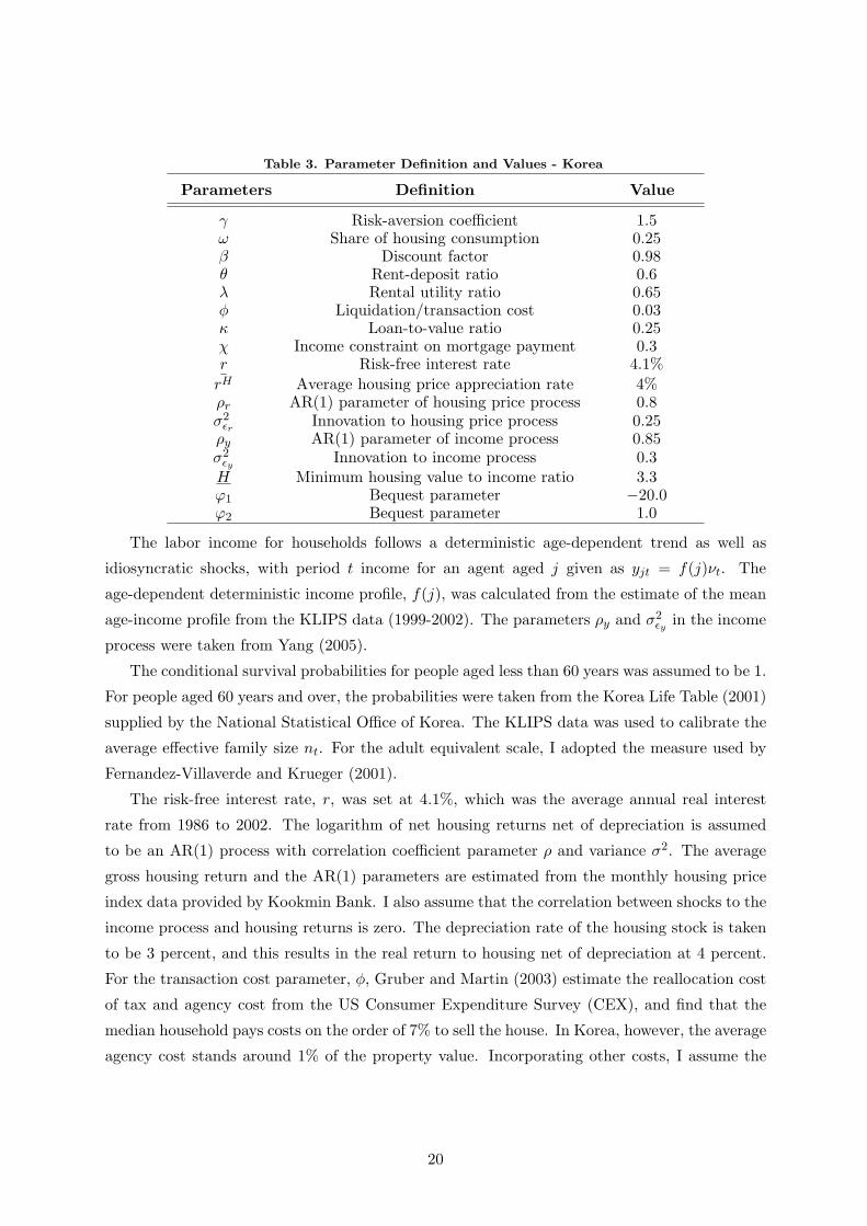
Table 3. Parameter Definition and Values - Korea
Parameters Definition Value
γ Risk-aversion coefficient 1.5ω Share of housing consumption 0.25β Discount factor 0.98θ Rent-deposit ratio 0.6λ Rental utility ratio 0.65φ Liquidation/transaction cost 0.03κ Loan-to-value ratio 0.25χ Income constraint on mortgage payment 0.3r Risk-free interest rate 4.1%
rH Average housing price appreciation rate 4%ρr AR(1) parameter of housing price process 0.8σ2
εrInnovation to housing price process 0.25
ρy AR(1) parameter of income process 0.85σ2
εyInnovation to income process 0.3
H Minimum housing value to income ratio 3.3ϕ1 Bequest parameter −20.0ϕ2 Bequest parameter 1.0
The labor income for households follows a deterministic age-dependent trend as well as
idiosyncratic shocks, with period t income for an agent aged j given as yjt = f(j)νt. The
age-dependent deterministic income profile, f(j), was calculated from the estimate of the mean
age-income profile from the KLIPS data (1999-2002). The parameters ρy and σ2εy
in the income
process were taken from Yang (2005).
The conditional survival probabilities for people aged less than 60 years was assumed to be 1.
For people aged 60 years and over, the probabilities were taken from the Korea Life Table (2001)
supplied by the National Statistical Office of Korea. The KLIPS data was used to calibrate the
average effective family size nt. For the adult equivalent scale, I adopted the measure used by
Fernandez-Villaverde and Krueger (2001).
The risk-free interest rate, r, was set at 4.1%, which was the average annual real interest
rate from 1986 to 2002. The logarithm of net housing returns net of depreciation is assumed
to be an AR(1) process with correlation coefficient parameter ρ and variance σ2. The average
gross housing return and the AR(1) parameters are estimated from the monthly housing price
index data provided by Kookmin Bank. I also assume that the correlation between shocks to the
income process and housing returns is zero. The depreciation rate of the housing stock is taken
to be 3 percent, and this results in the real return to housing net of depreciation at 4 percent.
For the transaction cost parameter, φ, Gruber and Martin (2003) estimate the reallocation cost
of tax and agency cost from the US Consumer Expenditure Survey (CEX), and find that the
median household pays costs on the order of 7% to sell the house. In Korea, however, the average
agency cost stands around 1% of the property value. Incorporating other costs, I assume the
20

transaction cost to be 3% of the property value in Korea.
The loan-to-value ratio, κ, was taken from the average of the loan-to-value ratio between the
years 1996 and 2000 compiled by the Housing and Commercial Bank in Korea. The parameter
for the income constraint, χ, was taken to be 0.3, which is a widely used figure by the mortgage
lenders. The rent-deposit ratio, θ, was taken to be 0.6 which falls in the middle of 0.4 and
0.8, taken from the data. In Section 6, a sensitivity analysis is conducted on the rent-deposit
ratio, which shows that for both higher and lower values of rent-deposit ratios, the result is
robust. The rental utility parameter, λ, is calibrated to be 0.60. The minimum housing value
is calibrated such that the average homeownership ratio in the benchmark simulation matches
the KLIPS data.
Regarding the preference parameters, the relative risk aversion coefficient, γ, is taken from
Attanasio et. al.(1999). The share of housing consumption, ω, ranges from 0.15 (Chen) to 0.4
(Platania & Schlagenhauf) in the literature. The median value of 0.25 is used for the model.
Later, in the sensitivity analysis on the share of housing consumption, it is shown that the
results were not affected by the change in the value of ω. The discount factor, β, is calibrated
to match the peak level of the net worth profile.
For the bequest parameters, the amount of bequests left by each age group are estimated
using the survival probabilities and the wealth data, following the method proposed by Shimono,
Otsuki and Ishikawa (1999). Aggregating the amount of bequests over all ages, the annual flow
of bequest to wealth ratio is found to be 0.46%13. The figure is consistent with studies by
Horioka et. al (2000) showing that the bequest motives in East Asian countries are weaker than
in the United States. The bequest parameter, ϕ1, is chosen so that the bequest to wealth ratio
matches the data. As for ϕ2, which governs the degree to which bequests are considered luxury
goods, the value is chosen to match the variance of the estimated bequest.
5 Results and Policy Experiments
In this section, the results from the benchmark simulation are presented and the fit of the model
is evaluated. Next, the roles of the institutional factors, namely, the mortgage market and the
rental arrangements, are examined. Finally, using the benchmark simulation as a reference, a
policy experiment of introducing a pay-as-you-go (PAYG) social security system is presented
and the implications on wealth accumulation and portfolio composition are analyzed. All other
parameters were kept unchanged at the same value as made under the benchmark simulation.13Gale and Scholz (1994) estimate the annual flow of bequest to be 0.88% of the aggregate net worth using the
1983 wave of the Survey of Consumer Finances.
21

5.1 Benchmark Case
In the model, net worth is defined as (1− I)θp−1h+ Iph+(1+ r)a+ tr, which is the sum of the
housing asset and financial net worth plus any transfers received in the beginning of the period.
This series is plotted against net worth in the data. In addition, housing asset for homeowners,
Iph, is plotted against the housing asset in the data. For non-housing net worth, the sum of
rent deposit, other financial net worth, and transfers, (1− I)θp−1h + (1 + r)a + tr, are plotted
against the sum of financial net worth and other non-financial asset in the data. The results
from the benchmark simulation are shown in Figure 5.1 to 5.4.
0
1
2
3
4
5
6
under25 30-35 40-45 50-55 60-65 70-75 over 80
Age
Av
era
ge
in
co
me
= 1
BENCHMARK
DATA
Figure 5.1 Net Worth (Benchmark)
0
1
2
3
4
under25 30-35 40-45 50-55 60-65 70-75 over 80
Age
Av
era
ge
in
co
me
= 1
BENCHMARK
DATA
Figure 5.2 Housing Asset (Benchmark)
0
1
2
3
under25 30-35 40-45 50-55 60-65 70-75 over 80
Age
Av
era
ge
in
co
me
= 1
BENCHMARK
DATA
Figure 5.3 Non-housing Net Worth(Benchmark)
0%
20%
40%
60%
80%
100%
under25 30-35 40-45 50-55 60-65 70-75 over 80
Age
BENCHMARK
DATA
Figure 5.4 Homeownership Ratio(Benchmark)
The benchmark simulation captures some features of the data while missing some other
aspects. These features can be summarized as follows:
• To begin with, Table 4 below compares the aggregate statistics of the benchmark economy
and the data.Table 4. Aggregate Statistics for Benchmark Economy
Benchmark Economy KLIPS Data
Net Worth to Income Ratio 3.27 4.43Housing Asset to Net Worth Ratio 0.63 0.58Homeownership Ratio 0.62 0.60
22

• The profile of net worth in the benchmark simulation has a hump-shaped path over age,
and the peak of net worth profile matches the the data fairly well. However, the timing at
which the peak occurs is at the ages of 60-65 in the simulation, which is around ten to fifteen
years later than the peak shown in the data. In addition, the simulation under-estimates
the aggregate net worth in the data, especially for working age groups. The simulation
can only generate 75% of the aggregate net worth in the data. Since the model focuses
on the average household, it does not generate sufficient heterogeneity and skewness in
wealth distribution. This might partly explain why the net worth to income ratio is lower
than the data.
• The profile of the housing asset also matches the hump shaped pattern shown in the data,
and the peak of the profile matches that of the data fairly well. Once the peak is reached
at the ages of 55-60, the level of the housing asset steadily declines. In addition, the profile
of the housing asset is zero for households from ages 20 to 35 since the households all rent.
The model does not generate enough wealth for the younger households to afford their
own housing.
• Non-housing net worth in the simulation is also matches some of the lifecycle pattern
shown in the data. However, the profile in the simulation is not as smooth as what is
shown in the data. In the model, the profile of non-housing net worth first peaks in the
early thirties, as people save before buying a house. As households borrow to finance their
housing purchase, non-housing net worth declines during the ages of late 30s and early 40s.
This period overlaps with the period in which households accumulate housing assets. Once
households become homeowners, they start accumulating financial assets again mostly to
finance consumption after retirement. In the data, however, the profile of non-housing
net worth shows a hump-shaped pattern over the life cycle without any significant decline
before retirement.
• Homeownership ratio in the benchmark simulation follows a hump-shaped pattern over
the age groups and matches the average homeownership ratio in the data. However, it
shows a rapid overshooting during the late 30s and early 40s age group, as it jumps from
0 to around 75%. The model is thus unable to explain the positive homeownership ratio
of younger households in the data. Furthermore, under the benchmark simulation, all
households between ages 50 to 70 years are homeowners. In the age groups of 60 years or
higher, the homeownership ratio starts to drop, eventually reaching around 65% for the
terminal age group.
23

5.2 The Role of The Institutional Features
In this section, the quantitative roles played by the institutional features of the mortgage and
the rental market are analyzed. First, to highlight the role of mortgage system, the current
system was modified to resemble the mortgage system in the United States. In fact, the Korean
government recently introduced a full-fledged mortgage loan program similar to that in the
United States. Even though it is too early to assess the impact of this recent policy introduction,
modifying the model by incorporating mortgage loans may shed light on how households’ tenure
decision will be affected, as well as the overall portfolio composition of wealth over the life cycle.
One way to incorporate mortgage into the model is to introduce an asset from which people
can borrow against. However, given the existing number of state variables, adding another
state variable would only complicate further the computation without providing many beneficial
implications. Thus, instead of adding another state variable, the loan-to-value (LTV) ratio is
changed to 70% from the benchmark ratio of 25%. This implies that households can now finance
their home purchase with an upfront down-payment of only 30% of the value of the house.
It is also assumed that households with a mortgage can refinance and adjust their mortgage
balance without any adjustment cost. Relaxing the collateral constraint will enable households
to purchase a house earlier and accumulate more housing assets. Table 5 below compares the
aggregate statistics for the case when the mortgage system is expanded. The profile of various
wealth and the pattern of homeownership under the alternative mortgage system are shown in
Figure 5.5 to 5.8.
Table 5. Aggregate Statistics for Alternative Mortgage System
Benchmark Alternative Mortgage
Net Worth to Income Ratio 3.27 3.16Housing Asset to Net Worth Ratio 0.63 0.77Homeownership Ratio 0.62 0.73
0
1
2
3
4
5
6
under25 30-35 40-45 50-55 60-65 70-75 over 80
Age
Av
era
ge
in
co
me
= 1
BENCHMARK
MORTGAGE
Figure 5.5 Net Worth (Mortgage)
0
1
2
3
4
under25 30-35 40-45 50-55 60-65 70-75 over 80
Age
Av
era
ge
in
co
me
= 1
BENCHMARK
MORTGAGE
Figure 5.6 Housing Asset (Mortgage)
24

-1
0
1
2
3
under25 30-35 40-45 50-55 60-65 70-75 over 80
Age
Av
era
ge
in
co
me
= 1
BENCHMARK
MORTGAGE
Figure 5.7 Non-housing Net Worth(Mortgage)
0%
20%
40%
60%
80%
100%
under25 30-35 40-45 50-55 60-65 70-75 over 80
Age
BENCHMARK
MORTGAGE
Figure 5.8 Homeownership Ratio(Mortgage)
• The aggregate net worth does not change significantly when the mortgage system is ex-
panded. The aggregate net worth to income ratio falls by 3.3%. Across different age
groups, the level of net worth is lower for households that are starting to purchase hous-
ing. This corresponds to age groups 35-45 years.
• Households start accumulating housing assets earlier in the life cycle. Due to a more
relaxed collateral constraint and households’ preference for owner-occupied housing over
renting, the housing asset to net worth ratio increases from 0.63 to 0.77.
• Non-housing net worth in the mortgage simulation peaks in the late twenties age group
and then dips into the negative range. The first peak of the non-housing net worth takes
place one model period earlier under the expanded mortgage. Households borrow more
and accumulate debt during the periods in which they start buying houses. From the
late forties, however, people start paying off the mortgage debt and start accumulating
financial assets.
• Relaxing the collateral constraint enables households to become homeowners earlier in the
life cycle than under the benchmark case. For age groups 30-35 years, 18% of households
are able to become homeowners through mortgage, compared to 0% under the benchmark
case. Also 75% of all households of ages 35-40 are homeowners, compared to around 20%
under the benchmark case. Homeownership increases significantly with the fraction of
homeowners in the economy increasing by approximately 11 percentage points under the
expanded mortgage system.
Next, to document the importance of the rental system, the rental arrangements in the
benchmark model was modified to mimic the rental system in the United States. Under the
alternative rental market arrangement, renters pay periodic rental payment, where the annual
rental cost is assumed to be a fraction µ of the house value. I choose three different numerical
values of µ - 2%, 4%, and 6% - and examine the implications of changing the rental arrangement.
25

The detailed set up of the alternative rental market arrangement is shown in the appendix. Table
6 below compares the aggregate statistics under the alternative rental market arrangement, while
the profile of various wealth and the pattern of homeownership under the alternative rental
arrangements are shown in Figure 5.9 to 5.20.
Table 6. Aggregate Statistics for Alternative Rental Arrangement
Benchmark µ = 2% µ = 4% µ = 6%
Net Worth to Income Ratio 3.27 3.07 3.29 3.38Housing Asset to Net Worth Ratio 0.63 0.59 0.63 0.68Homeownership Ratio 0.62 0.55 0.63 0.69
0
1
2
3
4
5
6
under25 30-35 40-45 50-55 60-65 70-75 over 80
Age
Av
era
ge
in
co
me
= 1
BENCHMARK
ALTERNATIVE RENTAL -
2% annual rental cost
Figure 5.9 Net Worth(Alternative Rent - 2%)
0
1
2
3
4
under25 30-35 40-45 50-55 60-65 70-75 over 80
Age
Av
era
ge
in
co
me
= 1
BENCHMARK
ALTERNATIVE RENTAL -
2% annual rental cost
Figure 5.10 Housing Asset(Alternative Rent - 2%)
0
1
2
3
under25 30-35 40-45 50-55 60-65 70-75 over 80
Age
Avera
ge i
nco
me =
1
BENCHMARK
ALTERNATIVE RENTAL -
2% annual rental cost
Figure 5.11 Non-housing Net Worth(Alternative Rent - 2%)
0%
20%
40%
60%
80%
100%
under25 30-35 40-45 50-55 60-65 70-75 over 80
Age
BENCHMARK
ALTERNATIVE RENTAL -
2% annual rental cost
Figure 5.12 Homeownership Ratio(Alternative Rent - 2%)
26

0
1
2
3
4
5
6
under25 30-35 40-45 50-55 60-65 70-75 over 80
Age
Av
era
ge
in
co
me
= 1
BENCHMARK
ALTERNATIVE RENTAL -
4% annual rental cost
Figure 5.13 Net Worth(Alternative Rent - 4%)
0
1
2
3
4
under25 30-35 40-45 50-55 60-65 70-75 over 80
Age
Av
era
ge
in
co
me
= 1
BENCHMARK
ALTERNATIVE RENTAL -
4% annual rental cost
Figure 5.14 Housing Asset(Alternative Rent - 4%)
0
1
2
3
under25 30-35 40-45 50-55 60-65 70-75 over 80
Age
Avera
ge i
nco
me =
1
BENCHMARK
ALTERNATIVE RENTAL -
4% annual rental cost
Figure 5.15 Non-housing Net Worth(Alternative Rent - 4%)
0%
20%
40%
60%
80%
100%
under25 30-35 40-45 50-55 60-65 70-75 over 80
Age
BENCHMARK
ALTERNATIVE RENTAL -
4% annual rental cost
Figure 5.16 Homeownership Ratio(Alternative Rent - 4%)
0
1
2
3
4
5
6
under25 30-35 40-45 50-55 60-65 70-75 over 80
Age
Av
era
ge
in
co
me
= 1
BENCHMARK
ALTERNATIVE RENTAL -
6% annual rental cost
Figure 5.17 Net Worth(Alternative Rent - 6%)
0
1
2
3
4
under25 30-35 40-45 50-55 60-65 70-75 over 80
Age
Av
era
ge
in
co
me
= 1
BENCHMARK
ALTERNATIVE RENTAL -
6% annual rental cost
Figure 5.18 Housing Asset(Alternative Rent - 6%)
0
1
2
3
under25 30-35 40-45 50-55 60-65 70-75 over 80
Age
Avera
ge i
nco
me =
1
BENCHMARK
ALTERNATIVE RENTAL -
6% annual rental cost
Figure 5.19 Non-housing Net Worth(Alternative Rent - 6%)
0%
20%
40%
60%
80%
100%
under25 30-35 40-45 50-55 60-65 70-75 over 80
Age
BENCHMARK
ALTERNATIVE RENTAL -
6% annual rental cost
Figure 5.20 Homeownership Ratio(Alternative Rent - 6%)
27

• The aggregate net worth to income ratio falls by 9.4% when the annual rental cost is set
to be 2%, while it remains almost unchanged when the rental cost is 4% of the house
value. For higher rental cost of 6%, however, the aggregate net worth to income ratio
increases by approximately 3.3%. Lower wealth accumulation for lower rental cost reflects
the decreased needs for savings in the earlier stage of life cycle geared towards housing
purchase.
• When the annual rental cost was set to be 2% of the house value, renting becomes relatively
cheaper in comparison to the benchmark case. This is shown in the two different stages of
the life cycle. First, for households in the forties age group, the conversion from renting to
homeownership takes place more slowly than in the benchmark case as they delay home
purchase. Second, more retired households switch back to renters as they find renting a
cheaper alternative to homeownership. As a result, the overall homeownership ratio falls
by 7 percentage points. Due to lower homeownership, the fraction of wealth invested into
housing asset also decreases by 4 percentage points.
• On the other hand, for higher annual rental costs, renting becomes a more expensive option
for households as they start becoming homeowners earlier and stay as homeowners after
retirement. When the rental cost was set to be 6% of the house value, households start
becoming homeowners earlier. For age groups 35-40, 60% of households decide to become
homeowners, compared to 20% in the benchmark case. The overall homeownership ratio
rises by 7 percentage points, while the fraction of wealth invested into housing assets
increases by 5 percentage points.
Finally, when the mortgage system and the rental arrangement are jointly modified, the
effects on housing wealth and homeownership ratio are further amplified, whereas the effect on
the overall net worth becomes negative for all possible arrangements. Table 7 below compares
the aggregate statistics for the case when both the rental arrangement and the mortgage system
are altered. The profile of various wealth and the pattern of homeownership under the alternative
mortgage and rental arrangement are shown in Figure 5.21 to 5.32.
Table 7. Aggregate Statistics under Alternative Mortgage and Rental Arrangement
Benchmark µ = 2% + µ = 4% + µ = 6% +Mortgage Mortgage Mortgage
Net Worth to Income Ratio 3.27 2.96 3.13 3.20Housing Asset to Net Worth Ratio 0.63 0.73 0.78 0.80Homeownership Ratio 0.62 0.66 0.74 0.77
28

0
1
2
3
4
5
6
under25 30-35 40-45 50-55 60-65 70-75 over 80
Age
Av
era
ge
in
co
me
= 1
BENCHMARK
ALTERNATIVE RENTAL(2%) &
MORTGAGE
Figure 5.21 Net Worth(Alternative Mortgage & Rent - 2%)
0
1
2
3
4
under25 30-35 40-45 50-55 60-65 70-75 over 80
Age
Av
era
ge
in
co
me
= 1
BENCHMARK
ALTERNATIVE RENTAL(2%) &
MORTGAGE
Figure 5.22 Housing Asset(Alternative Mortgage & Rent - 2%)
-1
0
1
2
3
under25 30-35 40-45 50-55 60-65 70-75 over 80
Age
Avera
ge i
nco
me =
1
BENCHMARK
ALTERNATIVE RENTAL(2%) &
MORTGAGE
Figure 5.23 Non-housing Net Worth(Alternative Mortgage & Rent - 2%)
0%
20%
40%
60%
80%
100%
under25 30-35 40-45 50-55 60-65 70-75 over 80
Age
BENCHMARK
ALTERNATIVE RENTAL(2%) &
MORTGAGE
Figure 5.24 Homeownership Ratio(Alternative Mortgage & Rent - 2%)
0
1
2
3
4
5
6
under25 30-35 40-45 50-55 60-65 70-75 over 80
Age
Av
era
ge
in
co
me
= 1
BENCHMARK
ALTERNATIVE RENTAL(4%) &
MORTGAGE
Figure 5.25 Net Worth(Alternative Mortgage & Rent - 4%)
0
1
2
3
4
under25 30-35 40-45 50-55 60-65 70-75 over 80
Age
Av
era
ge
in
co
me
= 1
BENCHMARK
ALTERNATIVE RENTAL(4%) &
MORTGAGE
Figure 5.26 Housing Asset(Alternative Mortgage & Rent - 4%)
-1
0
1
2
3
under25 30-35 40-45 50-55 60-65 70-75 over 80
Age
Avera
ge i
nco
me =
1
BENCHMARK
ALTERNATIVE RENTAL(4%) &
MORTGAGE
Figure 5.27 Non-housing Net Worth(Alternative Mortgage & Rent - 4%)
0%
20%
40%
60%
80%
100%
under25 30-35 40-45 50-55 60-65 70-75 over 80
Age
BENCHMARK
ALTERNATIVE RENTAL(4%) &
MORTGAGE
Figure 5.28 Homeownership Ratio(Alternative Mortgage & Rent - 4%)
29

0
1
2
3
4
5
6
under25 30-35 40-45 50-55 60-65 70-75 over 80
Age
Av
era
ge
in
co
me
= 1
BENCHMARK
ALTERNATIVE RENTAL(6%) &
MORTGAGE
Figure 5.29 Net Worth(Alternative Mortgage & Rent - 6%)
0
1
2
3
4
under25 30-35 40-45 50-55 60-65 70-75 over 80
Age
Av
era
ge
in
co
me
= 1
BENCHMARK
ALTERNATIVE RENTAL(6%) &
MORTGAGE
Figure 5.30 Housing Asset(Alternative Mortgage & Rent - 6%)
-1
0
1
2
3
under25 30-35 40-45 50-55 60-65 70-75 over 80
Age
Avera
ge i
nco
me =
1
BENCHMARK
ALTERNATIVE RENTAL(6%) &
MORTGAGE
Figure 5.31 Non-housing Net Worth(Alternative Mortgage & Rent - 6%)
0%
20%
40%
60%
80%
100%
under25 30-35 40-45 50-55 60-65 70-75 over 80
Age
BENCHMARK
ALTERNATIVE RENTAL(6%) &
MORTGAGE
Figure 5.32 Homeownership Ratio(Alternative Mortgage & Rent - 6%)
• The aggregate net worth to income ratio falls when alternative mortgage and rental ar-
rangements are jointly considered due to either wider availability of mortgage loans or
cheaper rental arrangements. For higher rental costs, the effect of mortgage expansion
dominates that of higher rental cost, thus lowering the overall level of savings in the econ-
omy. The aggregate net worth declines by 2.2% to 9.5%.
• Expanding mortgage system makes it easier for households to purchase housing, which
affects younger households more than older households. For all possible arrangements, the
homeownership of households of age groups 30-45 are all higher than the benchmark case,
regardless of the relative price of rental housing to owner-occupied housing.
• For all possible arrangements, the overall homeownership ratio increases, ranging from 4
percentage points to 15 percentage points increase. In addition, the overall housing asset
to net worth ratio increases for all possible housing market arrangements.
5.3 Pay-as-you-go (PAYG) Social Security Experiment
Finally, the impact of introducing a pay-as-you-go social security system is analyzed. Two
main motives for households to accumulate wealth over the life cycle are housing purchase and
30

retirement. In the previous section, the impact of changes in the housing market on the profile
of wealth and homeownership were examined. On the other hand, since it is hard to separate the
two saving motives, it would be interesting to see how the wealth portfolio and homeownership
decisions will be affected when the retirement arrangements are altered. To introduce social
security in the simplest manner, I assume that in each period working households from ages
20 to 55 years pay social security tax at a fixed rate, τ . The government collects the tax and
distributes social security benefits to the retirees at a constant replacement rate of $. The
social security payroll tax rate of 9% is taken from the Korean social security system, and the
implied replacement rate turns out to be 40%. Table 8 compares some aggregate properties of
the economy under the social security experiment with the benchmark economy. The results
from introducing a pay-as-you-go social security system are shown in Figure 5.33 to 5.36.
Table 8. Aggregate Statistics for Social Security Experiment
Benchmark Social Security
Net Worth to Income Ratio 3.27 2.92Housing Asset to Net Worth Ratio 0.63 0.64Homeownership Ratio 0.62 0.56
0
1
2
3
4
5
6
under25 30-35 40-45 50-55 60-65 70-75 over 80
Age
Av
era
ge
in
co
me
= 1
BENCHMARK
SOCIAL SECURITY
Figure 5.33 Net Worth (Social Security)
0
1
2
3
4
under25 30-35 40-45 50-55 60-65 70-75 over 80
Age
Av
era
ge
in
co
me
= 1
BENCHMARK
SOCIAL SECURITY
Figure 5.34 Housing Asset (Social Security)
0
1
2
3
under25 30-35 40-45 50-55 60-65 70-75 over 80
Age
Av
era
ge
in
co
me
= 1
BENCHMARK
SOCIAL SECURITY
Figure 5.35 Non-housing Net Worth(Social Security)
0%
20%
40%
60%
80%
100%
under25 30-35 40-45 50-55 60-65 70-75 over 80
Age
BENCHMARK
SOCIAL SECURITY
Figure 5.36 Homeownership Ratio(Social Security)
31

• The magnitude of the hump in net worth over the life cycle becomes smaller with the peak
of the net worth profile standing around 80% of the peak under the benchmark simulation.
Across different age groups, the decline in the level of net worth starts becoming more
prominent for ages 45 years or higher, as households have weaker motives to save for
retirement in the presence of social security system. Aggregating over all age groups, the
net worth to income ratio falls by around 10.3%.
• Weakening the households’ savings motive for retirement also has implications on the
accumulation of housing assets. Less wealth accumulation early in the life cycle implies
lower accumulation of housing assets at a reduced pace. Weaker need for savings to
finance consumption after retirement is also reflected in the lower level of accumulation in
the non-housing net worth, as the peak of non-housing asset at the time of retirement is
approximately 60% of the level in the absence of social security system.
• The homeownership ratio increases at a slower pace than under the benchmark simula-
tion. For age groups 40-45 years, approximately 60% of households become homeowners,
compared to 75% under the benchmark case. Introduction of a social security system neg-
atively affects the homeownership, as the average homeownership ratio falls to 56% from
62% in the benchmark economy.
6 Sensitivity Analysis
In this section, the robustness of the main findings in the benchmark economy to the choice of
key parameters are scrutinized. First, the rent-deposit ratio, θ, is changed for the sensitivity
analysis. Next, the share of housing consumption ω is checked. Finally, the effect of changing the
coefficient of relative risk aversion γ is rationalized. Other calibrated parameters are adjusted
accordingly to match the target variables in the data.
6.1 Rent-Deposit Ratio (θ)
In the data, the value of rental housing ranges from 40% to 80% of the purchasing value of
a house. In the benchmark, the median value was chosen. However, the actual value would
eventually depend on the supply and demand of the rental housing as opposed to owner-occupied
housing. Keeping this in mind, the effect of changing the rent-deposit ratio to a lower bound
of 40% and then to an upper bound of 80% on the profile of net worth and other assets were
evaluated. A lower value of θ implies that renting is relatively cheaper than buying a house.
This will make younger and older households stay in rental housing, which lowers the overall
32

homeownership ratio. For households aged 60 or above, the profile of housing assets and the
homeownership ratio declines more rapidly than the benchmark case. The profile of net worth
does not change significantly when the rent-deposit ratio is lowered to 40%. However, the profile
is slightly lower for the retired households, which reflects the fact that more households return
to renting. The results from changing θ to 40% are shown in Figure 6.1 to 6.4 in the Appendix.
On the other hand, when the value of θ is set at 80%, rental housing becomes relatively
more expensive. This makes it more attractive for the households to purchase housing earlier
in the life cycle and remain homeowners, as the de-cumulation of housing assets is slow after
retirement. The profile of various wealth and homeownership reflect this change in the relative
rental price. The evolution of the profile of net worth is similar to the profile in the benchmark
case. Figure 6.5 to 6.8 show the results when θ is changed to 80%.
6.2 Share of Housing Consumption (ω)
The parameter ω determines the share of housing consumption. In the benchmark economy, ω
was taken to be 0.25, as it represents a median value over the range used in the literature. The
profile of various wealth and the pattern of homeownership is examined when ω is changed to
a value of 0.2 and 0.3, respectively. A lower share of housing consumption at 0.2 implies that
households spend more on non-durable consumption and less on housing consumption. This
implies that housing as an asset becomes less attractive for households. In fact, households hold
less wealth in the form of housing assets. Also the overall level of net worth declines slightly
for all age groups. Given the adjustment in the calibrated parameters, however, the pattern
of homeownership remained similar to the benchmark case. For retired households aged over
65 years, housing asset de-cumulates is faster and the homeownership declines more rapidly
than the benchmark case, as older households place less weight on housing consumption during
retirement. The results from changing ω to 0.2 are shown in Figure 6.9 to 6.12.
On the contrary, when ω is changed to 0.3, the opposite effect takes place. The profile
of housing assets remains high even after retirement as households place more weight on the
consumption of housing goods. The overall profiles of net worth and financial net worth are
similar to those under the benchmark economy, as shown in Figure 6.13 to 6.16.
6.3 Relative Risk Aversion (γ)
In this subsection, the robustness of the results are checked when the value of γ, the relative risk
aversion parameter, is changed. Note that 1γ is the intertemporal elasticity of substitution. The
value of γ was increased from 1.5 to 2.5, lowering the intertemporal elasticity of substitution for
consumption. Thus, households become less willing to postpone consumption and therefore save
33

less in the immediate sense. The profile of net worth clearly verifies this effect as the level of
net worth is lower for households below the age of 45. The profile of the housing assets shows a
more risk-averse pattern. Even though the purchase of housing remains unchanged, households
begin to sell their houses more quickly after retirement. The homeownership ratio also shows
similar trend, with households over the age 60 or above quickly reverting to renting. Higher
risk aversion to income and housing returns uncertainties make households hold more riskfree
financial assets or stay as renters. Figure 6.17 to 6.20 show the results when γ is increased to
2.5.
7 Conclusion
In this paper, the wealth accumulation and asset portfolios of Korean households are investigated
by setting up a quantitative model calibrated to reflect some key features of the Korean economy.
The unique institutional features of the Korean housing market are highlighted and their roles
are examined. The chonsae system, the unique rental arrangement in Korea, and the lack of
mortgage system in Korea do play a significant role in accounting for the observed features
of wealth accumulation and portfolio composition in Korea. Also, the various implications of
recent policy changes are analyzed, such as expanding the current mortgage loan system and
introducing social security system to the economy. An expansion of the mortgage system is
expected to increase the average homeownership ratio significantly, especially for households in
the 30-40 age group; whereas, introducing social security has the opposite effect. Expanding the
mortgage system also shifts households’ wealth portfolio toward housing assets, while the social
security system does not affect the asset portfolio of households.
It is important to note that the model abstracts from several issues. Data shows significant
heterogeneity in households’ wealth portfolios in terms of age and income. For example, the
richest households have a disproportionately large share of the total wealth. However, the model
presented in this paper does not allow for this difference, since it concentrates on the average
household. Incorporating models of wealth inequality may help shed light on these issues and
improve the model.
In addition, the model does not incorporate the existence of inter-vivos transfers, which
might explain why the model underestimates the level of wealth for the young households and
is unable to match the age at which the profile of wealth peaks. In the data, Korean parents
provide large financial support to their children, especially when they become independent and
buy a house. Given the high down payment ratio, children either save for an extended period
of time or receive parental support in order to purchase a house. It is also reported that the
34

average inter-vivos transfers received as a fraction of average income is higher in Korea than
in the United States, especially for the younger households. This strengthens the importance
of inter-vivos transfers in Korea and their implications on the accumulation of wealth over the
lifecycle. Incorporating inter-vivos transfers in explaining the pattern of wealth accumulation in
Korea raises several challenging questions for future research.
35

References
[1] Ambrose, Brent W., and Sunwoong Kim. 2003. “Modeling the Korean Chonsei Lease
Contract, Real Estate Economics, vol.31, pp. 53-74.
[2] Attanasio, Orazio, James Banks, Costas Meghir and Guglielmo Weber. 1999. “Humps and
Bumps in Lifetime Consumption,” Journal of Business and Economics, 17, 22-35.
[3] Banks, James, Richard Blundell and James P. Smith. 2002. “Wealth Portfolios in the UK
and the US,” Working Paper No.9128, National Bureau of Economic Research, Cambridge,
MA.
[4] Campbell, John Y and Joao Cocco. 2003. Household Risk Management and Optimal Mort-
gage Choice, Working Paper, Harvard University. Cambridge, MA.
[5] Caroll, Christopher D. and Wendy E. Dunn. 1997. “Unemployment Expectations, Jumping
(S,s) Triggers, and Household Balance Sheets,” NBER Macroeconomics Annual 1997.
[6] Chambers, Matthew, Carlos Garriga and Don E. Schlagenhauf. 2004. “Accounting for
Changes in the Homeownership Rate,” Working paper, Florida State University.
[7] Chen, Kaiji. 2004. “The Welfare Implications of Social Security for Homeowners,” Job
Market Paper, University of Southern California, CA.
[8] Cho, Dongchul. 2005. “Interest Rate, Inflation, and Housing Price: With an Emphasis on
Chonsei Price in Korea,” Working Paper 11054, National Bureau of Economic Research,
Cambridge, MA.
[9] Cocco, Joao. 2004. “Portfolio Choice in the Presence of Housing,” accepted to Review of
Financial Studies.
[10] De Nardi, Mariacristina. 2004. “Wealth Inequality and Intergenerational Links,” Review
of Economic Studies, 71, 734-768.
[11] Dıaz, Antonia and Marıa J. Luengo-Prado. 2002. “Precautionary Saving and Wealth Dis-
tribution with Durable Goods,” Working paper, Northeastern University.
[12] Fernandez-Villaverde, Jesus and Dirk Krueger. 2001. “Consumption and Saving over the
Life Cycle: How Important are Consumer durables?” Proceedings of the 2002 North Amer-
ican Summer Meetings of the Econometric Society.
36

[13] Flavin, Marjorie and Takashi Yamashita. 2002. “Owner-Occupied Housing and the Com-
position of the Household Portfolio Over the Life Cycle,” American Economic Review, 92,
345-362.
[14] Glaeser, Edward L. and Jesse M. Shapiro. 2002. “The Benefits Of The Home Mortgage
Interest Deduction,” Working Paper No.9284, National Bureau of Economic Research,
Cambridge, MA.
[15] Goetzmann, William N., and Matthew Spiegel, 2002, “The Policy Implications of Portfolio
Choice in Underserved Mortgage Markets,” Low- Income Ownership, Joint Center for
Housing Studies, Brookings Institution Press, Washington D.C.. Eds. Retsinas and Belsky.
[16] Grossman, Sanford and Guy Laroque. 1990. “Asset Pricing and Optimal Portfolio Choice
in the Presence of Illiquid Housing Consumption Goods, Econometrica, 58, 25-51.
[17] Gruber, Joseph and Robert F. Martin. 2003. “The Role of Durable Goods in the Distri-
bution of Wealth: Does Housing Make Us Less Equal?” Working Paper.
[18] Guiso, Luigi, Michael Haliassos and Tullio Japelli, eds. 2002. Household Portfolios, MIT
Press, Cambridge, MA
[19] Haurin, Donald, Wenli Li and Rui Yao. 2004. “A Life-Cycle Model of Housing and Mort-
gage Choices with Labor Income and House Price Risks,” mimeo
[20] Horioka, Charles Yuji, Hideki Fujisaki, Wako Watanabe, and Takassugu Kouno. 2000. “Are
Americans More Altruistic Than The Japanese? A U.S.- Japan Comparison of Saving
and Bequest Motives,” Working Paper No.7463, National Bureau of Economic Research,
Cambridge, MA.
[21] Hu, Xiaoqing. 2003. “Portfolio Choices for Homeowners,” mimeo.
[22] Iwaisako, Takuo. 2003. “Household Portfolios in Japan,” Working Paper No.9647, National
Bureau of Economic Research, Cambridge, MA.
[23] Kennickell, Arthur. 2003. “A Rolling Tide: Changes in the Distribution of Wealth in the
U.S., 1989-2001,” SCF Working Paper, Federal Reserve Board.
[24] Keister, Lisa. 2000. Wealth in America : Trends in Wealth Inequality, Cambridge Univer-
sity Press, Cambridge, MA.
[25] Kim, Kyung-Hwan. 2004. “Housing and the Korean Economy,” Journal of Housing Eco-
nomics, Vol. 13, 321-341.
37

[26] Lam, Eddie. 2002. “A Primer for Investors in the Korean MBS Market,” Journal of Real
Estate Portfolio Management, Vol. 8, No. 2.
[27] Lee, Jungwoo and Sunglim Lee. 2001. “Estimation of Wealth Inequality in Korea (in
Korean),” Journal of Korean Development Economics, 7-1.
[28] Li, Wenli and Rui Yao. 2005. “The Life-Cycle Effects of House Price Changes,” Working
Paper No.05-7, Federal Reserve Bank of Philadelphia, Philadelphia, PA.
[29] Lucas, Jr., Robert E. 1987.Models of Business Cycles, Basil Blackwell, New York.
[30] McCarthy, David. 2004. “Household Portfolio Allocation: A Review of the Literature,”
mimeo.
[31] Miles, David, Ales Cerny and Lubomir Schmidt. 2004. “A Calibrated Model of Saving,
Portfolio Allocation and Housing Choices for Japanese Households,” mimeo.
[32] Ortalo-Magne, Francois and Sven Rady. 1998. “Housing Market Fluctuations in a Life-
Cycle Economy with Credit Constraints,” working paper, Graduate School of Business,
Stanford University.
[33] Platania, Jennifer and Don E. Schlagenhauf. 2002. “Housing and Asset Holding in a Dy-
namic General Equilibrium Model,” Working Paper, Florida State University.
[34] Shimono, Keiko, Hideaki Otsuki and Miho Ishikawa. 1999. “Estimating the Size and Dis-
tribution of Bequests in Japan,” mimeo, Institute of Economic Research, Nagoya City
University, Nagoya, Japan.
[35] Tauchen, George and Robert Hussey. 1991. “Quadrature-Based Methods for Obtaining
Approximate Solutions to Nonlinear Asset Pricing Models,” Econometrica, 59, 371-396.
[36] Yang, Fang. 2005. “Consumption Along the Life Cycle? How Different Is Housing?”
Working Paper No. 635, Federal Reserve Bank of Minneapolis, Minneapolis, MN.
[37] Yao, Rui and Harold H. Zhang. 2003. “Optimal Consumption and Portfolio Choices with
Risky Housing and Borrowing Constraints,” Working Paper, University of North Carolina.
38

Appendix: Alternative Arrangement in the Rental Market
To capture the rental system in the United States, a periodic rent payment is introduced, where
renters pay a fraction µ of the market value of the house, as well as a security deposit, which
is equivalent to a one month rental payment (denoted as a fraction ι of the housing value).14 I
show the arrangement for the value function for the household that chooses to rent in the next
period. In the beginning of period s, the household receives labor income, y, and transfers, tr,
depending on the working status and bequest eligibility status, respectively. If the household
is a renter during this period, then the renter receives the security deposit, a fraction ι of the
house value, from the landlord. If the household is a homeowner, then the homeowner receives
the value of housing with returns net of depreciation and liquidation cost. The household also
receives the financial net worth with realized riskfree returns. The available resource for the
household that chooses to rent in next period is denoted as follows:
WR = Iwy + (1− I)ιph + I(1− φ)ph + (1 + r)a + Iwtr
Given the available resources, the household then chooses consumption of non-durable goods,
c, financial net worth, a′, and pays periodic rental payment, µph′, which is a fraction µ of the
house value. If a renter moves to another rental housing, then the renter needs to pay a security
deposit on the new rental housing, denoted as ιph′. If the renter decides to stay at the current
rental housing, then h′ = h and there is no need for additional security deposit. Renters are not
allowed to borrow. In addition, upon retirement, the household faces a positive probability of
death, in which case the sum of financial net worth and rental payment in the next period are
left as a bequest b. Finally, non-negativity conditions hold for durable and non-durable goods
consumption. The value function of the household that chooses to rent in the next period is
thus given as follows:
V R(j, h, a, I, p, y) = maxc,h′,a′
[U(c, h, n) + sjβE(V (j + 1, h′, a′, I ′ = 0, p′, y′)) + (1− sj)ϕ(b)
]
subject to
c + a′ + µph′ + ιph′ ≤ WR
a′, c, h′ ≥ 0
b = a′ + (µ + ι)ph′
In the experiment, µ, the annual rental cost, ranged from 2% to 6% of the value of the house.
The security deposit ratio ι, is equivalent to a month rent payment, thus, 112th of the annual
rental cost.14I thank Javier Fernandez-Blanco for pointing this out.
39

Appendix: Computation of the Model
Since there is no closed form solution to the model, the model is solved numerically to work out
optimal decision rules at different ages as a function of the state variables (age, housing asset,
financial net worth, housing status, housing returns, and income). The optimal decision rules
were found by backward induction, starting at period T and working all the way to the initial
period.
In period T , the value functions coincide with the sum of the period utility function and
the bequest function, and, given the realization of the state variables, the consumption and
bequest choice is trivial. Based on the period T policy functions, in every period prior to T , the
values associated with the different choices of housing in the next period were calculated, and
consumption and asset portfolio choices conditional on different housing choices were obtained
subsequently.
For choices of control variables that violate various constraints, a large negative utility is
given so that an optimizing household would never opt for these choices. The realization of
stochastic housing returns and shocks to income are approximated using a two-state Markov
process following Tauchen and Hussey (1991). Shocks to housing returns were the same for each
cohort, while shocks to income were idiosyncratic. The state space for housing and financial
assets were discretized into a finite number of equally-spaced grid points. In the computation,
the number of points in the housing asset and financial net worth were 60 and 40, respectively.
Whenever the upper limit for the grids turned out to be binding in the solution to the
problem, the upper and lower bounds were increased and the problem was solved again. In the
end, the boundaries for the grids became sufficiently large and no longer imposed any constraint
on the optimization process. Having solved the model using the grid search method, a large
sample of different cohorts were simulated, and their optimal decisions over the life cycle were
recorded.
40

0
1
2
3
4
5
6
under25 30-35 40-45 50-55 60-65 70-75 over 80
Age
Av
era
ge
in
co
me
= 1
BENCHMARK
THETA = 0.4
DATA
Figure 6.1 Net Worth (θ = 0.4)
0
1
2
3
4
under25 30-35 40-45 50-55 60-65 70-75 over 80
Age
Av
era
ge
in
co
me
= 1
BENCHMARK
THETA = 0.4
DATA
Figure 6.2 Housing Asset (θ = 0.4)
0
1
2
3
under25 30-35 40-45 50-55 60-65 70-75 over 80
Age
Avera
ge i
nco
me =
1
BENCHMARK
THETA = 0.4
DATA
Figure 6.3 Non-housing Net Worth (θ = 0.4)
0%
20%
40%
60%
80%
100%
under25 30-35 40-45 50-55 60-65 70-75 over 80
Age
BENCHMARK
THETA = 0.4DATA
Figure 6.4 Homeownership Ratio (θ = 0.4)
0
1
2
3
4
5
6
under25 30-35 40-45 50-55 60-65 70-75 over 80
Age
Av
era
ge
in
co
me
= 1
BENCHMARK
THETA = 0.8
DATA
Figure 6.5 Net Worth (θ = 0.8)
0
1
2
3
4
under25 30-35 40-45 50-55 60-65 70-75 over 80
Age
Av
era
ge
in
co
me
= 1
BENCHMARK
THETA = 0.8
DATA
Figure 6.6 Housing Asset (θ = 0.8)
0
1
2
3
under25 30-35 40-45 50-55 60-65 70-75 over 80
Age
Av
era
ge
in
co
me
= 1
BENCHMARK THETA = 0.8
DATA
Figure 6.7 Non-housing Net Worth (θ = 0.8)
0%
20%
40%
60%
80%
100%
under25 30-35 40-45 50-55 60-65 70-75 over 80
Age
BENCHMARK
THETA = 0.8DATA
Figure 6.8 Homeownership Ratio (θ = 0.8)
41

0
1
2
3
4
5
6
under25 30-35 40-45 50-55 60-65 70-75 over 80
Age
Av
era
ge
in
co
me
= 1
BENCHMARK
OMEGA = 0.2DATA
Figure 6.9 Net Worth (ω = 0.2)
0
1
2
3
4
under25 30-35 40-45 50-55 60-65 70-75 over 80
Age
Av
era
ge
in
co
me
= 1
BENCHMARK
OMEGA = 0.2
DATA
Figure 6.10 Housing Asset (ω = 0.2)
0
1
2
3
under25 30-35 40-45 50-55 60-65 70-75 over 80
Age
Av
era
ge
in
co
me
= 1
BENCHMARK
OMEGA = 0.2
DATA
Figure 6.11 Non-housing Net Worth (ω = 0.2)
0%
20%
40%
60%
80%
100%
under25 30-35 40-45 50-55 60-65 70-75 over 80
Age
BENCHMARK
OMEGA = 0.2DATA
Figure 6.12 Homeownership Ratio (ω = 0.2)
0
1
2
3
4
5
6
under25 30-35 40-45 50-55 60-65 70-75 over 80
Age
Av
era
ge
in
co
me
= 1
BENCHMARK
OMEGA = 0.3
DATA
Figure 6.13 Net Worth (ω = 0.3)
0
1
2
3
4
under25 30-35 40-45 50-55 60-65 70-75 over 80
Age
Av
era
ge
in
co
me
= 1
BENCHMARK
OMEGA = 0.3
DATA
Figure 6.14 Housing Asset (ω = 0.3)
-1
0
1
2
3
under25 30-35 40-45 50-55 60-65 70-75 over 80
Age
Av
era
ge
in
co
me
= 1
BENCHMARK
OMEGA = 0.3
DATA
Figure 6.15 Non-housing Net Worth (ω = 0.3)
0%
20%
40%
60%
80%
100%
under25 30-35 40-45 50-55 60-65 70-75 over 80
Age
BENCHMARK
OMEGA = 0.3
DATA
Figure 6.16 Homeownership Ratio (ω = 0.3)
42

0
1
2
3
4
5
6
under25 30-35 40-45 50-55 60-65 70-75 over 80
Age
Av
era
ge
in
co
me
= 1 BENCHMARK
GAMMA = 2.5
DATA
Figure 6.17 Net Worth (γ = 2.5)
0
1
2
3
4
under25 30-35 40-45 50-55 60-65 70-75 over 80
Age
Av
era
ge
in
co
me
= 1
BENCHMARK
GAMMA = 2.5
DATA
Figure 6.18 Housing Asset (γ = 2.5)
-1
0
1
2
3
under25 30-35 40-45 50-55 60-65 70-75 over 80
Age
Av
era
ge
in
co
me
= 1
BENCHMARK
GAMMA = 2.5
DATA
Figure 6.19 Non-housing Net Worth (γ = 2.5)
0%
20%
40%
60%
80%
100%
under25 30-35 40-45 50-55 60-65 70-75 over 80
Age
BENCHMARK
GAMMA = 2.5
DATA
Figure 6.20 Homeownership Ratio (γ = 2.5)
43
Related Documents


![Final Program Report [Draft] · 2017. 5. 1. · THE FACULTY OF LAW UNIVERSITY OF NEW SOUTH WALES UNSW SYDNEY NSW 2052 December 2015 – December 2016 Final Program Report [Draft]](https://static.cupdf.com/doc/110x72/6124d1ba73608e64381a872b/final-program-report-draft-2017-5-1-the-faculty-of-law-university-of-new.jpg)