Geophys. J. Int. (2007) 168, 551–570 doi: 10.1111/j.1365-246X.2006.03233.x GJI Marine geoscience Scholte-wave tomography for shallow-water marine sediments Simone Kugler, 1 Thomas Bohlen, 2, ∗ Thomas Forbriger, 3, † Sascha Bussat 1 and Gerald Klein 4, ‡ 1 Kiel University, Institute of Geosciences, Geophysics, Otto-Hahn-Platz 1, 24118 Kiel, Germany. E-mail:[email protected] 2 Formerly Kiel University, Institute of Geosciences 3 Black Forest Observatory (BFO), Institute of Geosciences, Research Facility of the Universities of Karlsruhe and Stuttgart, Heubach 206, D-77709 Wolfach 4 Formerly IFM-Geomar, Wischhofstr. 1-3, 24148 Kiel, Germany Accepted 2006 September 22. Received 2006 September 21; in original form 2006 April 26 SUMMARY We determine the 3-D in situ shear-wave velocities of shallow-water marine sediments by ex- tending the method of surface wave tomography to Scholte-wave records acquired in shallow waters. Scholte waves are excited by air-gun shots in the water column and recorded at the seafloor by ocean-bottom seismometers as well as buried geophones. Our new method com- prises three steps: (1) We determine local phase-slowness values from slowness-frequency spectra calculated by a local wavefield transformation of common-receiver gathers. Areal phase-slowness maps for each frequency used as reference in the following step are obtained by interpolating the values derived from the local spectra. (2) We infer slowness residuals to those reference slowness maps by a tomographic inversion of the phase traveltimes of fun- damental Scholte-wave mode. (3) The phase-slowness maps together with the residuals at different frequencies define a local dispersion curve at every location of the investigation area. From those dispersion curves we determine a model of the depth-dependency of shear-wave ve- locities for every location. We apply this method to a 1 km 2 investigation area in the Baltic Sea (northern Germany). The phase-slowness maps obtained in step (2) show lateral variation of up to 150 per cent. The shear-wave velocity models derived in the third step typically have very low values (60–80 m s −1 ) in the top four meters where fine muddy sands can be observed, and values exceeding 170 m s −1 for the silts and sands below that level. The upper edge of glacial till with shear-wave velocities of 300–400 m s −1 is situated approximately 20 m below sea bottom. A sensitivity analysis reveals a maximum penetration depth of about 40 m below sea bottom, and that density may be an important parameter, best resolvable with multimode inversion. Key words: Surface waves, Scholte waves, dispersion, tomography, inversion, shear-wave velocity, shallow marine seismics 1 INTRODUCTION The determination of reliable 3-D models of shear-wave velocity for shallow-water marine sediments has applications in many differ- ent fields. The shear-wave velocity provides important information to characterize the sediment because it is much more sensitive to lithology variations, and less to fluid content than P-wave velocities are (Ayres & Theilen 1999; Hamilton 1976). The seafloor stabil- ity can be quantified by empirical relation between shear strength ∗ Now at: TU Bergakademie Freiberg, Gustav-Zeuner-Str. 12, 09596 Freiberg, Germany. †Also at: Geophysical Institute, University of Karlsruhe, Hertzstr. 16, D- 76187 Karlsruhe, Germany. ‡Now at: develogic GmbH, Theodorstr. 42-90, Haus 4a, 22761 Hamburg, Germany. and shear-wave velocity of the sediment (Ayres & Theilen 1999). 3-D shear-wave velocity models thus provide important informa- tion for geotechnical applications like the foundation of offshore platforms or pipelines or the investigation of slope stability. Fur- thermore, in combination with P-wave velocity, Poisson’s ratio can be inferred, which has been used to evaluate the porosity of the sediment (e.g. Hamilton 1976; Gaiser 1996). Multicomponent acquisition and processing of marine seismic data generally benefits from the knowledge about S-wave veloci- ties of the sediment. Especially in the first ten’s of meters beneath the seafloor significant changes in S-wave velocities over small dis- tances are commonly observed (Ewing et al. 1992; Stoll et al. 1994; Bohlen et al. 2004) which strongly effect processing algorithms for multicomponent seismic data like static corrections for SH -waves or converted PS-waves (Mari 1984; Muyzert 2000), wavefield separa- tion (e.g. Schalkwijk et al. 2000), as well as imaging with converted waves (Tatham & Goolsbee 1984). C 2006 The Authors 551 Journal compilation C 2006 RAS Downloaded from https://academic.oup.com/gji/article/168/2/551/688059 by guest on 14 February 2022

Welcome message from author
This document is posted to help you gain knowledge. Please leave a comment to let me know what you think about it! Share it to your friends and learn new things together.
Transcript
Geophys. J. Int. (2007) 168, 551–570 doi: 10.1111/j.1365-246X.2006.03233.x
GJI
Mar
ine
geos
cien
ce
Scholte-wave tomography for shallow-water marine sediments
Simone Kugler,1 Thomas Bohlen,2,∗ Thomas Forbriger,3,† Sascha Bussat1
and Gerald Klein4,‡1Kiel University, Institute of Geosciences, Geophysics, Otto-Hahn-Platz 1, 24118 Kiel, Germany. E-mail:[email protected] Kiel University, Institute of Geosciences3Black Forest Observatory (BFO), Institute of Geosciences, Research Facility of the Universities of Karlsruhe and Stuttgart, Heubach 206, D-77709 Wolfach4Formerly IFM-Geomar, Wischhofstr. 1-3, 24148 Kiel, Germany
Accepted 2006 September 22. Received 2006 September 21; in original form 2006 April 26
S U M M A R YWe determine the 3-D in situ shear-wave velocities of shallow-water marine sediments by ex-tending the method of surface wave tomography to Scholte-wave records acquired in shallowwaters. Scholte waves are excited by air-gun shots in the water column and recorded at theseafloor by ocean-bottom seismometers as well as buried geophones. Our new method com-prises three steps: (1) We determine local phase-slowness values from slowness-frequencyspectra calculated by a local wavefield transformation of common-receiver gathers. Arealphase-slowness maps for each frequency used as reference in the following step are obtainedby interpolating the values derived from the local spectra. (2) We infer slowness residuals tothose reference slowness maps by a tomographic inversion of the phase traveltimes of fun-damental Scholte-wave mode. (3) The phase-slowness maps together with the residuals atdifferent frequencies define a local dispersion curve at every location of the investigation area.From those dispersion curves we determine a model of the depth-dependency of shear-wave ve-locities for every location. We apply this method to a 1 km2 investigation area in the Baltic Sea(northern Germany). The phase-slowness maps obtained in step (2) show lateral variation ofup to 150 per cent. The shear-wave velocity models derived in the third step typically have verylow values (60–80 m s−1) in the top four meters where fine muddy sands can be observed, andvalues exceeding 170 m s−1 for the silts and sands below that level. The upper edge of glacial tillwith shear-wave velocities of 300–400 m s−1 is situated approximately 20 m below sea bottom.A sensitivity analysis reveals a maximum penetration depth of about 40 m below sea bottom,and that density may be an important parameter, best resolvable with multimode inversion.
Key words: Surface waves, Scholte waves, dispersion, tomography, inversion, shear-wavevelocity, shallow marine seismics
1 I N T RO D U C T I O N
The determination of reliable 3-D models of shear-wave velocityfor shallow-water marine sediments has applications in many differ-ent fields. The shear-wave velocity provides important informationto characterize the sediment because it is much more sensitive tolithology variations, and less to fluid content than P-wave velocitiesare (Ayres & Theilen 1999; Hamilton 1976). The seafloor stabil-ity can be quantified by empirical relation between shear strength
∗Now at: TU Bergakademie Freiberg, Gustav-Zeuner-Str. 12, 09596Freiberg, Germany.†Also at: Geophysical Institute, University of Karlsruhe, Hertzstr. 16, D-76187 Karlsruhe, Germany.‡Now at: develogic GmbH, Theodorstr. 42-90, Haus 4a, 22761 Hamburg,Germany.
and shear-wave velocity of the sediment (Ayres & Theilen 1999).3-D shear-wave velocity models thus provide important informa-tion for geotechnical applications like the foundation of offshoreplatforms or pipelines or the investigation of slope stability. Fur-thermore, in combination with P-wave velocity, Poisson’s ratio canbe inferred, which has been used to evaluate the porosity of thesediment (e.g. Hamilton 1976; Gaiser 1996).
Multicomponent acquisition and processing of marine seismicdata generally benefits from the knowledge about S-wave veloci-ties of the sediment. Especially in the first ten’s of meters beneaththe seafloor significant changes in S-wave velocities over small dis-tances are commonly observed (Ewing et al. 1992; Stoll et al. 1994;Bohlen et al. 2004) which strongly effect processing algorithms formulticomponent seismic data like static corrections for SH-waves orconverted PS-waves (Mari 1984; Muyzert 2000), wavefield separa-tion (e.g. Schalkwijk et al. 2000), as well as imaging with convertedwaves (Tatham & Goolsbee 1984).
C© 2006 The Authors 551Journal compilation C© 2006 RAS
Dow
nloaded from https://academ
ic.oup.com/gji/article/168/2/551/688059 by guest on 14 February 2022
552 S. Kugler et al.
Different seismic wave types can be analysed to study the shear-wave velocity structure of marine sediments. The application ofinterface waves provides many advantages over body shear-waves,especially in marine environments (Klein et al. 2005; Kugler et al.2005). We analyse the dispersive interface wave travelling alongthe interface between water and sediment, generally called Scholtewave (e.g. Rauch 1986) or generalized Rayleigh wave. Like Rayleighwaves (travelling along an air-solid interface) and Stonley waves(near a solid–solid interface) it is a P-SV polarized interface waveand shows significant sensitivity to shallow shear-wave velocity.Its propagation velocity is slightly lower than that of a Rayleighwave for small wavelengths and gradually approaches the Rayleigh-wave velocity for long wavelengths. So in the long-wavelength limit,the influence of the water-layer is negligible and the Scholte waveequals the Rayleigh wave. For smaller wavelengths it is a modifiedversion of the Rayleigh wave that is trapped near the fluid-solidinterface.
Compared to shear waves it has the advantage that it can be gen-erated with sufficient amplitude by an air-gun source in the watercolumn (Ritzwoller & Levshin 2002; Klein 2003; Bohlen et al. 2004)even for soft sediments which allows a fast data acquisition. Fur-thermore, because of the geometrical spreading of interface wavesbeing 2-D, the amplitude decrease with distance is less severe. Sincelonger wavelength fundamental Scholte waves have a larger pene-tration depth than those of shorter wavelengths elastic parametersas a function of depth can be estimated by recording a broad rangeof frequencies.
Scholte-wave dispersion has been previously used to determinethe lateral variation of shear-wave velocity of shallow-marine sed-iments. The analysis of local dispersion as a first step to the 2-DS-wave velocity model was performed by Stoll et al. (1994) throughcross multiplication of adjacent channels of a multichannel record.Others used different local wavefield transformation methods(Allnor et al. 1997; Muyzert 2000; Bohlen et al. 2004) which havethe main advantage that different Scholte-wave modes can be re-solved.
In global seismology the 3-D velocity structure of the crust andupper mantle is examined very successfully by surface wave to-mography since the 1970’s. A 3-D shear-wave velocity model wasderived, for example, by Woodhouse & Dziewonski (1984) usinga waveform inversion which assumes surface waves to propagatealong the great-circle avoiding the direct measurement of groupand phase velocities. Global group- and phase-velocity maps havebeen inferred for example by Nakanishi & Anderson (1982, 1983)by measuring the dispersion of fundamental-mode surface waves.Later, as the number of digital seismic records increased, the con-struction of global models with higher resolution (e.g. Trampert &Woodhouse 1995) as well as regional investigations (e.g. Ritzwoller& Levshin 1998) became possible. Ray theory has played a centralrole in most of this research. In recent years the use of scatteringtheory based on the Born or Rytov approximation became popularin seismological surface-wave tomography to overcome the limita-tions of ray theory (e.g. Meier et al. 1997; Friederich 1999; Spetzleret al. 2002; Snieder 2002; Ritzwoller et al. 2002). The studies ap-proximate the effects of surface-wave propagation in heterogeneousmedia to a different degree, following diverse approaches concern-ing single or multiple scattering and the treatment of mode couplingand conversion.
The conditions and questions found in shallow seismics, however,differ significantly from earthquake seismology restricting the rangeof methods that are adapted for shallow application. In shallow seis-mics no a priori reference model is available like in global seismic
studies, where only relatively small perturbations to a well estab-lished reference model have to be determined. Furthermore strongermodel parameter variations commonly exist, where large velocitycontrasts and reversals can lead to higher mode propagation. Theresponse-function of the receiver in shallow seismics, especially ifit is deployed as an ocean-bottom seismometer on a soft seafloor, isnot known without in situ calibration because of unknown seafloorcoupling. On the other hand, shallow seismic investigations havethe advantage that the positions of sources and receivers and thusthe path coverage are not as restricted as in seismology. With regardto the geotechnical application in shallow marine environments amethod is needed that allows a fast and robust estimate of the 3-Dshear-wave velocity structure with a minimum of a priori informa-tion needed.
Until today the investigations of near-surface shear-wave veloc-ities using surface waves have usually been restricted to 2-D. 3-D areal mapping in shallow land seismics was accomplished byBadal et al. (2004) by simply spatially interpolating between a num-ber of 1-D phase velocity soundings over the study area. Rigorous3-D mapping by tomography has been conducted by Dombrowski(1996) as well as Long & Kocaoglu (2001). Dombrowski recordedRayleigh waves along many different ray paths across his study area.He determined the group velocity for each ray path by a modifiedwavelet transform dispersion analysis. From all group velocities hefinally inferred group velocity maps using a standard traveltime to-mography. He interpreted the lateral group velocity variations of thetomograms, without inverting them to shear-wave velocity models.Long & Kocaoglu used a standard multiple filter technique to mea-sure group velocities along many different ray paths. Then they alsoapplied a tomographic inversion method to obtain the distributionof group velocities inside that study area. The shear-wave velocitystructure of the study area was determined from the group velocitydispersion curves by the inverse method outlined by Kocaoglu &Long (1993).
In this work, we analyse the phase-traveltimes of Scholte waves.We assume that the phase velocity of the Scholte mode at each pointon its path equals the structural velocity as defined from the materialparameters of the underlying medium. The work of Wielandt (1993),however, showed that this is only the case for plane waves.
We adapt the concept of surface wave phase-traveltime tomog-raphy to shallow-water marine environments using fundamentalScholte waves, which are excited by an air-gun source and recordedby ocean-bottom seismometers, after the approach of Bohlen et al.(2004) to derive fundamental mode phase slowness dispersion alongstraight lines in the investigation area. These phase slowness mea-surements are used to construct a coarse phase slowness modelneeded as background model in the following tomographic inver-sion. To linearize the problem, we assume that the Scholte wavetravels along the direct path connecting source and receiver. Themethod basically consists of three major steps: First we construct aphase slowness background model for each frequency. In the sec-ond step we infer deviations from the background model throughtomographic inversion of phase traveltimes, so we are able to con-struct improved phase slowness maps. The improved maps containthe areal Scholte-wave dispersion which we invert in the third stepfor the local 1-D shear-wave velocity variation with depth at eachsurface element of the area.
The paper is organised as follows: First we describe the dispersionanalysis, phase traveltime tomography and inversion to 3-D shear-wave velocity. Subsequently, we present the field data and describethe data acquisition and geometry. We then infer a 1-D subsurfacemodel and background phase-slowness maps before we describe
C© 2006 The Authors, GJI, 168, 551–570
Journal compilation C© 2006 RAS
Dow
nloaded from https://academ
ic.oup.com/gji/article/168/2/551/688059 by guest on 14 February 2022

Scholte-wave tomography 553
the application of our tomographic approach. Finally we present theresulting 3-D shear-wave velocity model.
2 M E T H O D S
2.1 First step: Local wavefield transformation
The objective of local wavefield transformation is to identify thephase slowness of all Scholte-wave modes excited by the source fora narrowly limited subsurface region. To achieve this, the recordedwavefield is transformed from the offset-time domain into theslowness-frequency domain. Methods of wavefield transformationare described by McMechan & Yedlin (1981), Park et al. (1998) andForbriger (2003a). They consist of two consecutive linear transfor-mations. McMechan & Yedlin (1981) suggest the application of aslant-stack (p,τ -transform) followed by a 1-D Fourier transform withrespect to τ . Park et al. (1998) and Forbriger (2003a) start with a 2-DFourier transform and perform the summation as the second step inthe frequency domain after applying an offset-dependent phase shift.Both methods generate a slowness-frequency spectrum (p–f spec-trum), where the dispersion relation becomes apparent through theamplitude maxima. To extract local phase slowness from a recordedwavefield the offset range of the transformed seismograms has tobe restricted. For this purpose successive pie-shaped phase-velocityfilters can be applied to the wavefield leading to velocity-frequencyspectra for each offset (Misiek 1996). Scholte waves were analysedwith this method by Muyzert (2000). Bohlen et al. (2004) suggestedthe calculation of local p–f spectra by local slant stacking, whichcontains a successive offset-dependent weighting of the traces bymultiplying with a Gaussian offset window before the actual trans-formation. However both methods suffer from the principal trade-offbetween the resolution in phase slowness and array aperture. Thisproblem also exists for the spectral representation of signals in aspectrogram, where it is desirable to obtain both a high temporaland spectral resolution, but due to the uncertainty principle for thetime-frequency representation of signals this is impossible there aswell.
We apply the method of local slant stack described and tested indetail by Bohlen et al. (2004) and here give a brief summary of theprocedure.
If the wavefield consists of N traces u(x k , t), recorded at theoffsets x k over the time t were k = 1, 2, . . . , N denotes the shotnumber, the local wavefield uc(x k , x c, t) can be calculated by themultiplication of the original wavefield u(x k , t) with a Gaussianoffset window
uc(xk, xc, t ; L) = u(xk, t) exp
[−
(xk − xc
L2
)2], (1)
where L/2 denotes the distance where the window amplitude dropsto 1/e and x c is the centre of the Gaussian offset window. Afterthis windowing, the local wavefield is transformed to the slowness-frequency domain through Fourier transformation
uc(xk, xc, f ) =∫ +∞
−∞uc(xk, xc, t)ei2π f t dt (2)
followed by an offset-dependent phase shift −2π fpxk and the sum-mation
Uc(xc, p, f ) =N∑
k=1
uc(xk, xc, f )e−i2π f pxk (3)
over all shots k, where Uc(xc, p, f ) is the complex p–f spectrum ofthe local wavefield for the central offset x c.
For the calculation of local slowness-frequency spectra (p–f spec-tra) from Common Receiver Gathers (CRGs) (alternatively Com-mon Shot Gathers (CSGs)) it is required that all receivers (shots) lieapproximately on one straight line with the shot (receiver) so thatthe difference between two adjacent seismograms is solely causedby the medium between the two appropriate shots (receivers). Formarine environments we favour the application of CRGs because itis much easier to shoot at many different air-gun source points ratherthan deploying a comparable number of ocean-bottom seismometerswith a single shot point. In the analysis of CRGs source repeatabil-ity is an important aspect. Furthermore, the distances between theshots have to be carefully chosen depending on the slowest expectedScholte-wave velocity to avoid spatial aliasing (Bohlen et al. 2004;Klein et al. 2005).
Bohlen et al. (2004) have shown that the dispersion curves ex-tracted from local p–f spectrum of a CRG solely depend on themedium within the analysis window. This gives us the possibility tomeasure the phase slowness of all excited Scholte-wave modes fordiscrete subsurface areas along profiles leading to a coarse back-ground phase-slowness model, which is necessary for the tomo-graphic inversion in the next step.
2.2 Second step: Phase traveltime tomography
In a second step we refine the coarse background model of localphase slowness by a tomographic approach. This uses data fromwaves that did not travel along the profiles from which local wave-field transforms were obtained.
We use a very simplified approach to surface wave propagationand assume (1) that we can separate a single Scholte mode fromthe rest of the wavefield in time domain, (2) that this mode can bedescribed by a plane wave travelling along a straight line betweensource and receiver, and (3) that the phase velocity of the mode ateach point on its path equals the structural velocity (Wielandt 1993)of the wave defined by the 1-D structure below that point.
Unfortunately reality differs from our assumptions, since: (1) in-terface wave propagation in shallow soil is in many cases dominatedby higher modes which interfere and are coupled due to hetero-geneity, and (2) the wave is generally not plane but has cylindricalsymmetry in homogeneous media and undergoes severe deviationsfrom cylindrical symmetry for laterally heterogeneous media dueto wavefield scattering. We expect most severe problems to be dueto the effect of lateral heterogeneity and the assumption that wavespropagate along a straight line. But in contrast to global seismicstudies, we are not seeking for small perturbations to a well estab-lished reference model. In shallow seismics, we believe that we cantolerate a bias of a few percent due to systematic insufficiency ofour approach. If we also require the wave path and the wave cur-vature to depend on structure of the medium, the inverse problemwould become non-linear. With our simple approach the solutionis linear and straightforward. A correct wave theoretical approachthat incorporates scattering (Friederich 1998) and mode coupling(Friederich 1999) would increase numerical effort by several ordersof magnitude and would not be applicable without a good referencemodel.
Let
ulm(t) =∫ ∞
−∞Alm( f ) ei�lm ( f ) e−2iπ f d f (4)
be the waveform of the Scholte mode that travelled from source lto receiver m. Alm( f ) ∈ R is then the modulus of its Fourier trans-form, which includes the magnitude of wave excitation and wave
C© 2006 The Authors, GJI, 168, 551–570
Journal compilation C© 2006 RAS
Dow
nloaded from https://academ
ic.oup.com/gji/article/168/2/551/688059 by guest on 14 February 2022
554 S. Kugler et al.
attenuation along the path, and
�lm( f ) = φRm( f ) + φS
l ( f ) + 2π f
∫Clm
p(x(s), f ) ds (5)
is the phase of its Fourier transform, which includes the phase delaydue to finite phase slowness p and phase contributions φS and φR bythe source and the receiver, respectively. C lm specifies the integrationpath along the straight line between source and receiver and x(s) arethe coordinates along the path. The phase slowness p(x (s), f ) thatcontrols wave propagation varies with location x and frequency f .It defines a dispersion relation at each location. The expression forthe phase contribution due to wave propagation is exact in the caseof plane waves propagating perpendicular to the boundaries of aband-like heterogeneity (Friederich et al. 1993).
For the purpose of inversion we distinguish between a mean con-tribution
plm( f ) = 1
xlm
∫Clm
p0(x(s), f ) ds (6)
that is already contained in the background model p0(x (s), f ) anda residual contribution δp(x(s), f ) = p(x(s), f ) − plm( f ). x lm =|xl − xm | is the distance between source and receiver. The back-ground model p0(x (s), f ) is derived from interpolating the phaseslowness of local wavefield transforms as is described later. Weremove the contribution plm from the recorded data urec
lm (t) by de-convolution. The deconvolved waveform
udeclm (t) =
∫ +∞
−∞urec( f ) e−2π i f plm ( f )xlm d f (7)
is derived by removing the phase contribution due to the backgroundmodel from the Fourier transform urec( f ) of the recorded waveform.From this representation it is possible to extract the Scholte modeunder investigation with a narrow taper. The bias contributed by thetaper was described by Wielandt & Schenk (1993) but is ignoredin our study, since it is smaller than the bias due to ignoring non-plane wave propagation. Furthermore, deconvolution is essentialfor determining the Fourier phase of the deconvolved signal udec
lm (t).Phase determination is always non-unique by an additive constant ofa multiple of 2π . While this happens to be a problem with �lm( f ) inparticular at large offsets, the phase of the deconvolved signal can beexpected to be less than 2π , if the background model is appropriateand if the mean contribution of source and receiver are removed too.For each source receiver combination we determine the phase
�declm ( f ) = atan
(Im(udec
lm ( f ))
Re(udeclm ( f ))
)(8)
of the deconvolved seismogram udeclm (t), with udec
lm ( f ) being theFourier transform of udec
lm (t). Thereby �declm ( f ) is expected to be in
the range from −π to +π . If this assumption is violated for thefield data, the background model could not explain the phase val-ues sufficiently and a phase unwrapping becomes necessary. Thephase unwrapping consists of two consecutive steps and is based onthe following assumptions: (1) The paths from two adjacent shotswithin a profile to one receiver differ only slightly, so that the phasedifference of the traces should be much smaller than 2π . This equalsthe spatial Nyquist criterion which already has to be fulfilled for ap-plying the local wavefield transformation when we determine thebackground model. (2) The background model fits the data to asimilar extent for all frequencies. Therefore, the phase values be-longing to two adjacent frequency samples differ only slightly. Thefirst step unwraps from shot to shot within one profile. Therefore,we minimize the function
F1(n) = ∣∣�declm ( f ) − �dec
(l+1),m( f ) − n2π∣∣, n ∈ Z (9)
and obtain nmin for which F 1 becomes minimal. The unwrappedphase can then be calculated from the original phase by
�dec(l+1)m, ( f ) = �dec
(l+1),m( f ) − nmin2π. (10)
This is done consecutively for all shots l within one profile withthe phase of the nearest shot to the receiver �dec
1,m( f ) = �dec1,m( f ) is
left unchanged. In the second step the unwrapping from frequencyto frequency is realized. If we have determined the phase �dec
lm forthe N f frequency samples f i (i = 1, . . . , N f ), we minimize thefunction
F2(n) =∣∣∣∣ ∑
l
�declm ( fi ) −
∑l
�declm ( fi+1) − n2π
∣∣∣∣, n ∈ Z (11)
where the sum is performed over all shots within one profile anddetermine nmin. Then we apply the same phase shift −nmin2π forall the shots l in the profile by
ˆ�
dec
lm ( fi+1) = �declm ( fi+1) − nmin2π. (12)
We repeat this second unwrapping for all frequency samples f i .This two-step phase unwrapping is done independently for allprofile-receiver combinations of the data set. Finally, we removethe average phase φ for every profile and get the remainingphase
φlm( fi ) = ˆ�
dec
lm ( fi ) − 1
Nshot
∑l
ˆ�
dec
lm ( fi ) (13)
Unfortunately in our case no data are available to determine thereceiver transfer function nor the source wavelet. We cannot distin-guish between both and hence combine them to a phase contributionφ P = φS + φR, which is assumed to be the same for all shots alongone profile P.
The φ lm( f ) are the data for the tomographic inversion. Unknownsare the δp(x (s), f ) describing lateral variation of dispersion and thephase contribution δφP = φP −φ due to the source and receiver. Thephase slowness map δ p(x (s), f ) + p0(x (s), f ) that characterizesthe structure under investigation is then obtained by minimizing theresidual
φlm( f ) − δφP ( f ) − 2π f
∫Clm
δp(x(s), f ) ds (14)
in a least-squares sense with respect to δφ P and δp(x (s), f ) for allsource and receiver combinations at once and for all frequencies,which is a linear problem.
In order to represent the tomographic model by a finite numberof unknowns, we use blocks as basis functions for the parametriza-tion of phase slowness. Thereby we divide the study area into binswith constant slowness. After discretization of the medium the inte-gral in eq. (14) simplifies to a summation. Furthermore, if we haverecorded seismograms at N R different receiver locations, excitedat N S different source locations we can set up a linear system ofequations of the form
dobs − Gm = dresidual, (15)
where dobs is a vector containing the remaining phases φ lm( f ) for allsource-receiver combinations at a given frequency and dresidual sig-nifies the residuals between data and prediction. The design matrixG accounts for the individual ray path and m is the vector containingthe unknowns
m( f ) = (δφP1( f ), δφP2( f ), . . . , δφP(NP +NR )( f ),
δp(r1, f ), . . . , δp(rM , f )), (16)
C© 2006 The Authors, GJI, 168, 551–570
Journal compilation C© 2006 RAS
Dow
nloaded from https://academ
ic.oup.com/gji/article/168/2/551/688059 by guest on 14 February 2022
Scholte-wave tomography 555
with N P denoting the number of profiles in the data set and Mbeing the number of bins in the study area with the coordinatesr1, . . . , rM . This is done independently for each frequency f so wehave dropped f in the notation.
We now search for the residuals m that fit the data in a least-squares sense (|dresidual|2 = min) by minimizing the objective func-tion
�(m) = (dobs − Gm)TCe(dobs − Gm) + mTQm, (17)
where Ce is a diagonal matrix weighting the input data dobs.The second term of the objective function (17) describes the
damping condition. With this condition a priori constraints for thesearched model are introduced. As we will show later, our dataset has regions where many ray paths intersect the bins while inother regions the data coverage is poor. This has to be balanced bythe damping condition so we include a model norm constraint thattakes data coverage into account. Furthermore a spatial smoothingconstraint is used. This is included in the damping matrix
Q = FTF + HTH, (18)
which is described with more generality by Barmin et al. (2001).Here
Fi j = γ
0, if (i, j ≤ N );
1, if (i, j > N ) ∨ (i = j);
−S(ri−N , r j−N )/gi−N , if (i, j > N ) ∨ (i �= j),
with gi−N = ∑j
S(ri−N , r j−N ).
(19)
is the spatial smoothing constraint with the indices i , j = 1, . . . , N+ M ; N = N P + N R and S denoting the smoothing Kernel
S(rm, rn) = exp
(− |rm − rn|2
2σ 2
)(20)
which includes the correlation length σ and n, m = 1, . . . , M .The smoothing constraint assures that the differences between thephase slowness residual δp of a bin and the weighted sum of thephase slowness residuals of all other bins is small. The weightingis thereby dependent on the spatial distance between the bins anddecreases with increasing distance like a Gaussian distribution withcorrelation length σ .
The model norm constraint is given by the matrix
Hi j =
α, if (i = j) ∨ (i ≤ N );
βe−λξi , if (i = j) ∨ (i > N );
0, if (i �= j),
(21)
where λ is a user-defined constant and i , j = 1, . . . , N + M . Thematrix H accounts for local path density ξ , that is, the number of raypaths intersecting a bin which will be described in detail later. Sincethe model vector m contains the perturbations of slowness froma background model the consideration of local path density in themodel norm constraint ensures that the estimated model merges intothe background model in areas of poor data coverage. The dampingconstants α and β specify the relative strength of damping betweenthe model parameters of remaining phase contribution δφ P due tosource and receiver and the slowness residuals δp. Furthermore thedamping constants β and γ define the relative strength of normconstraint and smoothing to the estimated model. They control thetrade-off between model amplitude and misfit. For the tomographicinversion of our data set, we find the optimal combination of damp-ing constants by trial inversions of synthetic data sets with manydifferent damping constants which is discussed in detail below.
We now set all partial derivatives of the objective function (17)with respect to the components of m to zero and obtain the matrixequation
mest = (GTCeG + Q)−1GTCedobs (22)
for the best-fitting residual phase slowness of the bins in the studyarea and residual phase contribution of source and receiver com-prised in mest.
To assess the resolution of the tomographic inversion we inferthe model resolution matrix (Menke 1989). Therefore, we substituteeq. (15) with dresidual = 0 into expression (22) and obtain
mest = (GTCeG + Q
)−1GTCeGm = Rm, (23)
with the symmetric model resolution matrix R. Each row of R sig-nifies to what extend the model parameters can actually be resolved.In the ideal case of perfect resolution the resolution matrix wouldequal the identity matrix.
2.3 Third step: Inversion
From the phase slowness maps pobs(r, f ) estimated by the describedtraveltime tomography we can extract local Scholte-wave dispersioncurves. From this input data, we determine the local S-wave velocityv s(r, z) as a function of depth z using the inversion scheme describedby Bohlen et al. (2004). Since Scholte-wave dispersion is in principalalso influenced by compressional-wave velocity and density, we willinvestigate the sensitivity of Scholte-wave dispersion to all seismicparameters for a single 1-D subsurface model that is representativefor our study site later. The influence of seismic wave attenuation tothe Scholte-wave dispersion can be neglected because the dispersioncaused by moderate Q-values (Q > 10) is small compared to thedispersion of the Scholte wave due to structural variations of elasticparameters in the subsurface.
We describe the subsurface by k discrete layers overlying a halfspace. The properties of each layer are defined by shear-wave veloc-ity v s , compressional-wave velocity v p , and density ρ of its top andbottom with a linear gradient in-between and the layer thickness (h)leading to the set of model parameters
η = (h, vs
top, vsbot, vp
top, vpbot,ρtop,ρbot, vhs
s , vhsp , ρhs
), (24)
where the vectors of the elastic parameters have k components andvhs
s , vhsp , ρhs define the elastic parameters in the half space. The
starting model of the inversion is guessed by testing many differentplausible models manually. The model with the best fit is then usedas starting model, whereas the number of layers is the minimumnumber which is able to explain the measured p–f spectrum. Fromsuch a subsurface model the synthetic p–f spectrum is calculatedby Wang’s method (Wang 1999). The phase slowness dispersionpmod(r, η, f i ) predicted by the model is obtained by automaticallypicking the maxima in the synthetic p–f spectrum (Bohlen et al.2004). We define the relative misfit to the input data pobs(r, f i ) bythe objective function:
�(η) = 1
n
n∑i=1
(pmod(r,η, fi ) − pobs(r, fi ))2, (25)
where n denotes the number of picked frequency values. The in-version is performed without damping of the model. For the op-timization of this nonlinear objective function we apply the Se-quential Quadratic Programming method (function ‘fmincon’ of theMATLAB optimization toolbox), which is described, for example,by Boggs & Tolle (1995). The partial derivatives are derived numer-ically by finite differences.
C© 2006 The Authors, GJI, 168, 551–570
Journal compilation C© 2006 RAS
Dow
nloaded from https://academ
ic.oup.com/gji/article/168/2/551/688059 by guest on 14 February 2022
556 S. Kugler et al.
3 F I E L D DATA S E T
3.1 Survey area
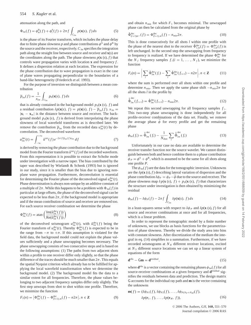
The study site is located in the Tromper Wiek, a bay situated in thenortheastern part of Rugen island (northern Germany). It is opento the Baltic Sea to the northeast (Fig. 1). Tromper Wiek formsa transition area between the onshore glaciotectonically deformeddeposits of Wittow, Jasmund and Schaabe on the one hand and therecent mud accumulation of the Arkona Basin on the other hand(Lemke et al. 1998). The recent water depth in the central part of
Figure 1. (a) Location of the Tromper Wiek in the Baltic Sea (north of Germany). (b) Locations of source points and receivers. The air gun was fired alongthe lines with shot spacings between 4 and 20 m. The circles denote the positions of OBS, the triangles of buried geophones. Records from the grey markedprofile P23 (2002) recorded by geophone 4 are shown in Fig. 3.
Tromper Wiek is about 20 m. Lemke et al. (1998) divide the sed-iment into five seismostratigraphic units on the basis of acousticalinvestigations and sediment core information. The uppermost till isassigned to the Weichselian glaciation and is situated approximately20 m below sea bottom. Its upper edge is structured by late glacialchannels filled with glaciolacustrine sediments of the early BalticIce Lake stages. These are overlain by silts or silty fine sands offreshwater origin from the final phase of the Baltic Ice Lake. In thecentral part of the bay the silts were covered by a younger unit offine muddy sand, which was deposited in the Ancylus Lake. With in-creasing water depth to the northeast, muddy Littorina Sea sediments
C© 2006 The Authors, GJI, 168, 551–570
Journal compilation C© 2006 RAS
Dow
nloaded from https://academ
ic.oup.com/gji/article/168/2/551/688059 by guest on 14 February 2022
Scholte-wave tomography 557
geophone1 msediment
water20 m
5 m
air gunOBS
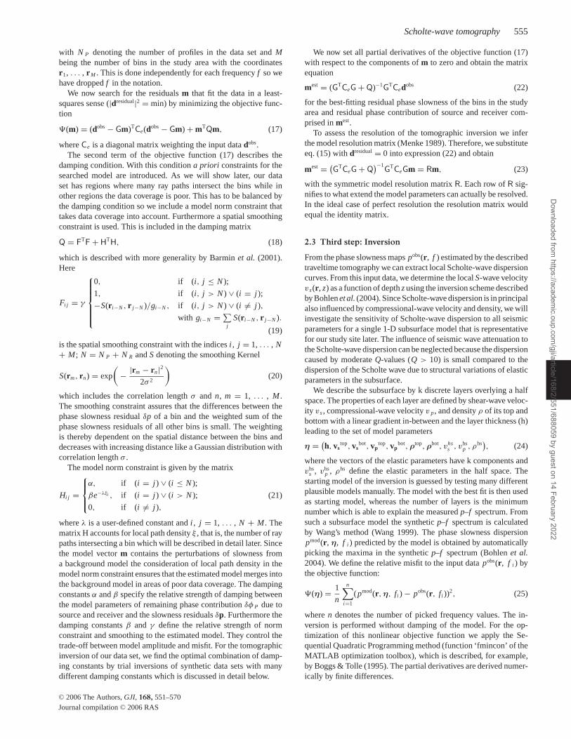
Figure 2. Acquisition parameters: Scholte waves were excited by airgunshots 5 m below sea level and recorded at the seafloor by ocean-bottomseismometers (OBS), as well as buried geophones. The water depth wasabout 20 m.
are observed. Our study area with the dimensions of approximately1 km × 1 km is situated in the central part of the Tromper Wiek.
3.2 Data acquisition and geometry
For this study, we generated Scholte waves by small airgun (0.6 litre)shots in the water layer approx. 5 m below sea level and recordedthem by ocean-bottom seismometers (OBS) as well as buried geo-phones (both with eigenfrequencies of 4 Hz) as indicated in Fig. 2.The airgun pulse had a centre frequency of approx. 35 Hz. The shotswere arranged along lines with shot distances between 4 and 20 mcovering the study area (Fig. 1b). Records from two surveys one yearapart were gathered to a data set of 40 000 records, assuming thatthe elastic parameters of the sediment did not change significantlyin the meantime. During the first survey in the year 2002 1250 shotswere recorded by 4 receivers followed by about 3000 shots recordedby 12 receivers in the year 2003. The shot locations were measuredby a differential GPS positioning system.
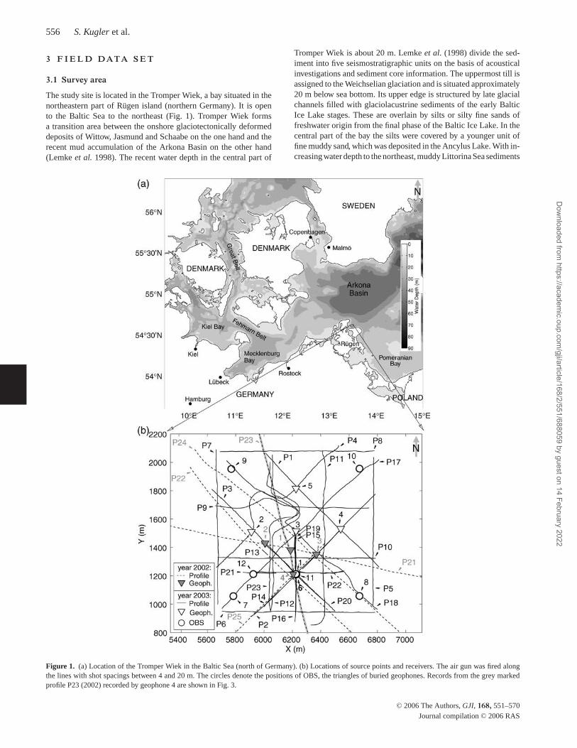
As an example, Fig. 3 shows a common receiver gather (CRG)recorded by the vertical component of geophone 4 (2002) for shots
0
1
2
3
4
5
6
7
Tim
e (s
)
-400 -300 -200 -100 0 100 200 300Distance (m)
mental
highermodes
Profile 23(2002), Geophone 4
SSE NNW
mode
Figure 3. Common receiver gather of profile 23 (2002) recorded by the vertical component of geophone 4 (2002). The traces are normalized to their maximumamplitude and low-pass filtered below 20 Hz. A strong dispersed fundamental Scholte mode as well as faster higher modes can be observed.
along profile 23 (2002). The seismograms are normalized to theirmaximum amplitude to correct for amplitude variation with off-set possibly caused by geometrical spreading, attenuation or sourcestrength variation. A low-pass frequency filter is applied at 20 Hzto reduce amplitudes of body waves and guided acoustic waves.The signal-to-noise-ratio of this CRG is one of the best obtainedin this survey. The records show a strong dispersed fundamentalScholte mode as well as higher mode amplitudes. The modes arenormally dispersed, that is, higher frequency components propagatewith smaller phase velocity. Seismograms with sufficient Scholte-wave energy for the following analysis were recorded up to 800 moffset.
4 O N E - D I M E N S I O N A L S U B S U R FA C EM O D E L A N D B A C KG RO U N D P H A S ES L O W N E S S
In a first step towards a 3-D shear-wave velocity model we derive afirst estimate of areal Scholte-wave phase slowness by local wave-field transformation along the profiles. In the middle of the studyarea we infer a 1-D subsurface model which was used to study thesensitivity of the Scholte-wave phase slowness to model variationsas well as model resolution.
4.1 One-dimensional inversion
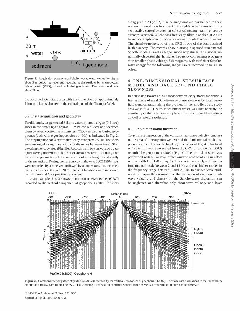
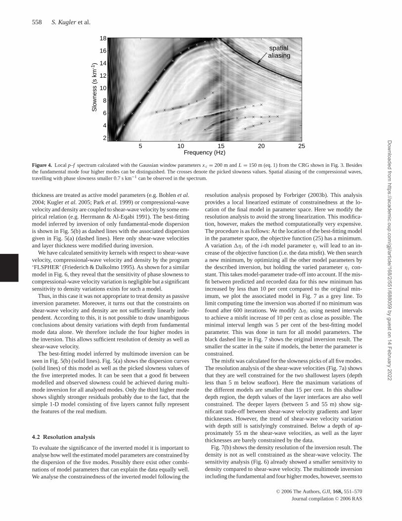
To get a first impression of the vertical shear-wave velocity structurein the area of investigation we inverted the fundamental mode dis-persion extracted from the local p–f spectrum of Fig. 4. This localp–f spectrum was determined from the CRG of profile 23 (2002)recorded by geophone 4 (2002) (Fig. 3). The local slant stack wasperformed with a Gaussian offset window centred at 200 m offsetwith a width L of 150 m (eq. 1). The spectrum clearly exhibits thefundamental mode between 2 and 15 Hz and four higher modes inthe frequency range between 5 and 22 Hz. In surface wave stud-ies it is frequently assumed that the influence of compressional-wave velocity and density on the Scholte-wave dispersion canbe neglected and therefore only shear-wave velocity and layer
C© 2006 The Authors, GJI, 168, 551–570
Journal compilation C© 2006 RAS
Dow
nloaded from https://academ
ic.oup.com/gji/article/168/2/551/688059 by guest on 14 February 2022
558 S. Kugler et al.
Frequency (Hz)
Slo
wne
ss (
s km
-1)
5 10 15 20 252
4
6
8
10
12
14
16
18
spatialaliasing
Figure 4. Local p–f spectrum calculated with the Gaussian window parameters x c = 200 m and L = 150 m (eq. 1) from the CRG shown in Fig. 3. Besidesthe fundamental mode four higher modes can be distinguished. The crosses denote the picked slowness values. Spatial aliasing of the compressional waves,travelling with phase slowness smaller 0.7 s km−1 can be observed in the spectrum.
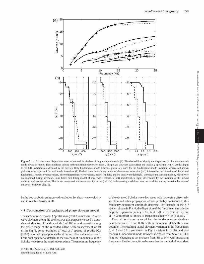
thickness are treated as active model parameters (e.g. Bohlen et al.2004; Kugler et al. 2005; Park et al. 1999) or compressional-wavevelocity and density are coupled to shear-wave velocity by some em-pirical relation (e.g. Herrmann & Al-Eqabi 1991). The best-fittingmodel inferred by inversion of only fundamental-mode dispersionis shown in Fig. 5(b) as dashed lines with the associated dispersiongiven in Fig. 5(a) (dashed lines). Here only shear-wave velocitiesand layer thickness were modified during inversion.
We have calculated sensitivity kernels with respect to shear-wavevelocity, compressional-wave velocity and density by the program‘FLSPHER’ (Friederich & Dalkolmo 1995). As shown for a similarmodel in Fig. 6, they reveal that the sensitivity of phase slowness tocompressional-wave velocity variation is negligible but a significantsensitivity to density variations exists for such a model.
Thus, in this case it was not appropriate to treat density as passiveinversion parameter. Moreover, it turns out that the constraints onshear-wave velocity and density are not sufficiently linearly inde-pendent. According to this, it is not possible to draw unambiguousconclusions about density variations with depth from fundamentalmode data alone. We therefore include the four higher modes inthe inversion. This allows sufficient resolution of density as well asshear-wave velocity.
The best-fitting model inferred by multimode inversion can beseen in Fig. 5(b) (solid lines). Fig. 5(a) shows the dispersion curves(solid lines) of this model as well as the picked slowness values ofthe five interpreted modes. It can be seen that a good fit betweenmodelled and observed slowness could be achieved during multi-mode inversion for all analysed modes. Only the third higher modeshows slightly stronger residuals probably due to the fact, that thesimple 1-D model consisting of five layers cannot fully representthe features of the real medium.
4.2 Resolution analysis
To evaluate the significance of the inverted model it is important toanalyse how well the estimated model parameters are constrained bythe dispersion of the five modes. Possibly there exist other combi-nations of model parameters that can explain the data equally well.We analyse the constrainedness of the inverted model following the
resolution analysis proposed by Forbriger (2003b). This analysisprovides a local linearized estimate of constrainedness at the lo-cation of the final model in parameter space. Here we modify theresolution analysis to avoid the strong linearization. This modifica-tion, however, makes the method computationally very expensive.The procedure is as follows: At the location of the best-fitting modelin the parameter space, the objective function (25) has a minimum.A variation �η i of the i-th model parameter η i will lead to an in-crease of the objective function (i.e. the data misfit). We then searcha new minimum, by optimizing all the other model parameters bythe described inversion, but holding the varied parameter η i con-stant. This takes model-parameter trade-off into account. If the mis-fit between predicted and recorded data for this new minimum hasincreased by less than 10 per cent compared to the original min-imum, we plot the associated model in Fig. 7 as a grey line. Tolimit computing time the inversion was aborted if no minimum wasfound after 600 iterations. We modify �η i using nested intervalsto achieve a misfit increase of 10 per cent as close as possible. Theminimal interval length was 5 per cent of the best-fitting modelparameter. This was done in turn for all model parameters. Theblack dashed line in Fig. 7 shows the original inversion result. Thesmaller the scatter in the suite if models, the better the parameter isconstrained.
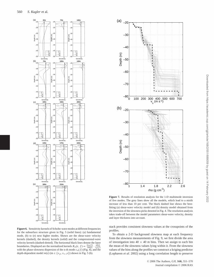
The misfit was calculated for the slowness picks of all five modes.The resolution analysis of the shear-wave velocities (Fig. 7a) showsthat they are well constrained for the two shallowest layers (depthless than 5 m below seafloor). Here the maximum variations ofthe different models are smaller than 15 per cent. In this shallowdepth region, the depth values of the layer interfaces are also wellconstrained. The deeper layers (between 5 and 55 m) show sig-nificant trade-off between shear-wave velocity gradients and layerthicknesses. However, the trend of shear-wave velocity variationwith depth still is satisfyingly constrained. Below a depth of ap-proximately 55 m the shear-wave velocities, as well as the layerthicknesses are barely constrained by the data.
Fig. 7(b) shows the density resolution of the inversion result. Thedensity is not as well constrained as the shear-wave velocity. Thesensitivity analysis (Fig. 6) already showed a smaller sensitivity todensity compared to shear-wave velocity. The multimode inversionincluding the fundamental and four higher modes, however, seems to
C© 2006 The Authors, GJI, 168, 551–570
Journal compilation C© 2006 RAS
Dow
nloaded from https://academ
ic.oup.com/gji/article/168/2/551/688059 by guest on 14 February 2022
Scholte-wave tomography 559
0 200 400 600
Dep
th (
m)
vs (m s-1)
1500 1750 200080
70
60
50
40
30
20
vp (m s-1)
1 1.4 1.8 2.2 2.680
70
60
50
40
30
20
ρ (g cm-3)
0 5 10 15 20 250
5
10
15
20
Frequency (Hz)
Slo
wne
ss (
s km
-1)
(a)
(b)
Figure 5. (a) Scholte wave dispersion curves calculated for the best-fitting models shown in (b). The dashed lines signify the dispersion for the fundamental-mode inversion model. The solid lines belong to the multimode inversion model. The picked slowness values from the local p–f spectrum (Fig. 4) used as inputto the 1-D inversions are denoted by the crosses. Only fundamental-mode slowness picks were used for the fundamental-mode inversion, whereas all shownpicks were incorporated for multimode inversion. (b) Dashed lines: best-fitting model of shear-wave velocities (left) inferred by the inversion of the pickedfundamental mode slowness values. The compressional-wave velocity model (middle) and the density model (right) shown are the starting models, which werenot modified during inversion. Solid lines: best-fitting model of shear-wave velocities (left) and densities (right) determined by the inversion of the pickedmultimode slowness values. The shown compressional-wave velocity model (middle) is the starting model and was not modified during inversion because ofthe poor sensitivity (Fig. 6).
be the key to obtain an improved resolution for shear-wave velocityand to resolve density at all.
4.3 Construction of a background phase-slowness model
The calculation of local p–f spectra is only valid to measure Scholte-wave slowness along the profiles. For that purpose we used a Gaus-sian window (eq. 1) with a width L of 100 m and moved it alongthe offset range of the recorded CRGs with an increment of 10m. In Fig. 8, some examples of local p–f spectra of profile P23(2002) recorded by geophone 4 for different offset values are shown.From such spectra we determine the slowness of fundamental modeScholte wave from the amplitude maxima. The maximum frequency
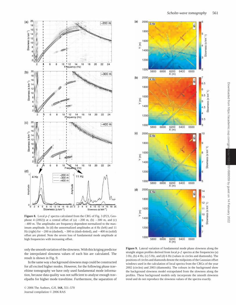
of the observed Scholte wave decreases with increasing offset. Ab-sorption and other propagation effects probably contribute to thisfrequency-dependent amplitude decrease. For instance in the p–fspectra shown in Fig. 8, the dispersion of the fundamental mode canbe picked up to a frequency of 16 Hz at −200 m offset (Fig. 8a), butat −400 m offset is limited to frequencies below 7 Hz (Fig. 8c).
From all local spectra we picked the fundamental mode slow-ness between 2 Hz and 8 Hz with an increment of 0.5 Hz wherepossible. The resulting lateral slowness variation at the frequencies3, 4, 5 and 6 Hz are shown in Fig. 9 (values in circles and dia-monds). Fundamental mode slowness increases from S to N at 3 Hz(Fig. 9a) changing to an increase from SE to NW with increasingfrequency. Furthermore, it can be seen that the method of local slant
C© 2006 The Authors, GJI, 168, 551–570
Journal compilation C© 2006 RAS
Dow
nloaded from https://academ
ic.oup.com/gji/article/168/2/551/688059 by guest on 14 February 2022
560 S. Kugler et al.
0
Dep
th (
m)
Sensitivity
10Hz
0
Dep
th (
m)
Sensitivity
15Hz
0
Dep
th (
m)
Sensitivity
20Hz
0
Dep
th (
m)
Sensitivity
13Hz
0
Dep
th (
m)
Sensitivity
17Hz
0
Dep
th (
m)
Sensitivity
22Hz
0
Dep
th (
m)
Sensitivity
21Hz
0
Dep
th (
m)
Dep
th (
m)
Dep
th (
m)
Dep
th (
m)
Dep
th (
m)
ρvvsp
Sensitivity
18Hz
ρvvsp
ρvvsp
ρvvsp
0Sensitivity
7Hz
ρvvsp
0
2Hz
Sensitivity
ρvvsp
ρvvsp
ρvvsp
ρvvsp
0Sensitivity
10Hz
ρvvsp
Sensitivity
7Hz
0
ρvvsp
ρvvsp
ρvvsp
0Sensitivity
14Hz
ρvvsp
0Sensitivity
14Hz
Dep
th (
m)
Dep
th (
m)
(d)
(c)
(e)
(b)
(a)
Figure 6. Sensitivity kernels of Scholte-wave modes at different frequenciesfor the subsurface structure given in Fig. 5 (solid lines): (a) fundamentalmode, (b) to (e) next higher modes. Shown are the shear-wave velocitykernels (dashed), the density kernels (solid) and the compressional-wavevelocity kernels (dashed-dotted). The horizontal black lines denote the layerboundaries. Displayed are the normalized kernels Kn(z, f ) = ∂cn ( f )
∂m(z) · m(z)cn ( f )
with the phase-slowness dispersion of the n-th mode cn( f ) (Fig. 4), and thedepth-dependent model m(z) (m ∈ {v p , v s , ρ}) shown in Fig. 5 (b).
0 100 200 300 400 500 600 700v
s (m s-1)
Dep
th (
m)
1 1.4 1.8 2.2 2.680
70
60
50
40
30
20
rho (g cm-3)
Dep
th (
m)
(a)
(b)
Figure 7. Results of resolution analysis for the 1-D multimode inversionof five modes. The grey lines show all the models, which lead to a misfitincrease of less than 10 per cent. The black dashed line shows the best-fitting (a) shear-wave velocity model and (b) density model obtained fromthe inversion of the slowness picks denoted in Fig. 4. The resolution analysistakes trade-off between the model parameters shear-wave velocity, densityand layer thickness into account.
stack provides consistent slowness values at the crosspoints of theprofiles.
To obtain a 2-D background slowness map at each frequencyfrom the slowness measurements of Fig. 9, we first divide the areaof investigation into 40 × 40 m bins. Then we assign to each binthe mean of the slowness values lying within it. From the slownessvalues of the bins along the profiles we construct a kriging predictor(Lophaven et al. 2002) using a long correlation length to preserve
C© 2006 The Authors, GJI, 168, 551–570
Journal compilation C© 2006 RAS
Dow
nloaded from https://academ
ic.oup.com/gji/article/168/2/551/688059 by guest on 14 February 2022
Scholte-wave tomography 561
Figure 8. Local p–f spectra calculated from the CRG of Fig. 3 (P23, Geo-phone 4 (2002)) at a central offset of (a) −200 m, (b) −300 m, and (c)−400 m. The amplitudes are frequency-dependent normalized to the max-imum amplitude. In (d) the unnormalized amplitudes at 4 Hz (left) and 11Hz (right) for −200 m (dashed), −300 m (dash-dotted), and −400 m (solid)offset are plotted. Note the severe loss of fundamental mode amplitude athigh frequencies with increasing offset.
only the smooth variation of the slowness. With this kriging predictorthe interpolated slowness values of each bin are calculated. Theresult is shown in Fig. 9.
In the same way a background slowness map could be constructedfor all excited higher modes. However, for the following phase trav-eltime tomography we have only used fundamental mode informa-tion, because data quality was not sufficient to analyse enough trav-elpaths for higher mode traveltime. Furthermore, the separation of
Figure 9. Lateral variation of fundamental mode phase slowness along thestraight airgun profiles derived from local p–f spectra at the frequencies (a)3 Hz, (b) 4 Hz, (c) 5 Hz, and (d) 6 Hz (values in circles and diamonds). Thepositions of circles and diamonds denote the midpoints of the Gaussian offsetwindows used in the calculation of local spectra from the CRGs of the year2002 (circles) and 2003 (diamonds). The colours in the background showthe background slowness model extrapolated from the slowness along theprofiles. These background models only incorporate the smooth slownesstrend and do not reproduce the slowness values of the spectra exactly.
C© 2006 The Authors, GJI, 168, 551–570
Journal compilation C© 2006 RAS
Dow
nloaded from https://academ
ic.oup.com/gji/article/168/2/551/688059 by guest on 14 February 2022
562 S. Kugler et al.
modes after deconvolution is generally difficult if their slownessvalues are too similar. For our data set we are able to extract fun-damental and first higher mode phase values from the deconvolvedtraces with high signal-to-noise ratio. The second to fourth highermode, however, could not sufficiently be separated, since their slow-ness values are too close together.
The 2-D inferred slowness maps (Fig. 9) can now be used as abackground slowness model for the application of the deconvolu-tion (eq. 7). Before deconvolution we must interpolate the back-ground slowness because we need to know a slowness value p0(r,f i ) for each frequency sample f i from 0 Hz to the Nyquist fre-quency. We use the described inversion from Scholte-wave p–f picksto shear-wave velocity model as such an interpolation method. Aspline interpolation method would, however, do as well. Data inputof the inversion are the background slowness values at the pickedfrequencies. The vector of model parameters η include layer thick-nesses and associated shear-wave velocities for five layers and theshear-wave velocity of the half space. Above the layered sedimentmodel, a water layer of 20 m thickness was implemented. For eachbin the slowness values were inverted for a best-fitting model η(r).From those models we calculate the background slowness for everyfrequency needed in the deconvolution (eq. 7).
5 P H A S E T R AV E LT I M E T O M O G R A P H Y
5.1 Data preprocessing
In preparation for the tomographic inversion we extract the residualphases φ lm( f i ) of fundamental Scholte wave from the deconvolvedseismic traces. We will explain the procedure applied to the seismo-grams from CRG P23 (2002) shown in Fig. 3.
By deconvolution we remove the dispersion due to the back-ground model p0(r, f i ). Prior to the application of the deconvolu-tion (eq. 7), it is important to extend the seismic traces to negativetimes since we apply a discrete Fourier transform to the data. Afterdeconvolution the fundamental mode dispersion is almost removedas can be seen in Fig. 10, while higher mode energy was moved to
-5
-4
-3
-2
-1
0
1
2
Tim
e (s
)
-300 -200 -100 0 100 200 300Distance (m)
Profile 23(2002), Geophone 4
NNWSSE
fundamental mode fundamental mode
higher modes higher modes
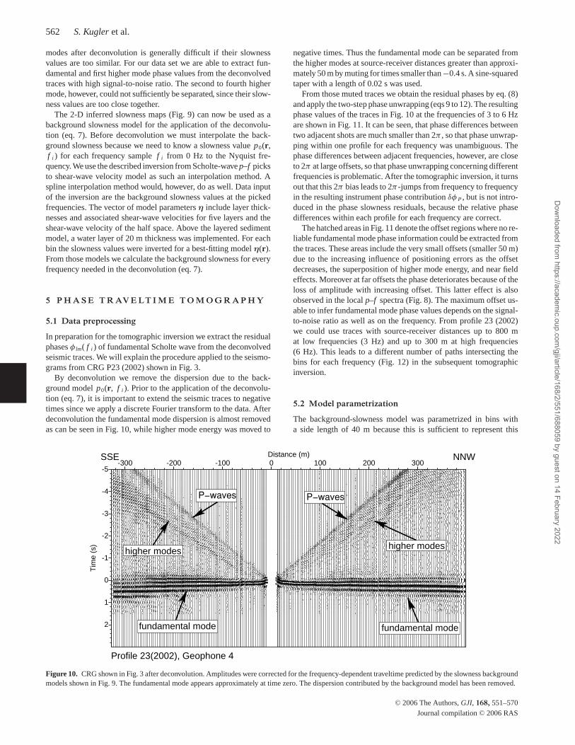
Figure 10. CRG shown in Fig. 3 after deconvolution. Amplitudes were corrected for the frequency-dependent traveltime predicted by the slowness backgroundmodels shown in Fig. 9. The fundamental mode appears approximately at time zero. The dispersion contributed by the background model has been removed.
negative times. Thus the fundamental mode can be separated fromthe higher modes at source-receiver distances greater than approxi-mately 50 m by muting for times smaller than −0.4 s. A sine-squaredtaper with a length of 0.02 s was used.
From those muted traces we obtain the residual phases by eq. (8)and apply the two-step phase unwrapping (eqs 9 to 12). The resultingphase values of the traces in Fig. 10 at the frequencies of 3 to 6 Hzare shown in Fig. 11. It can be seen, that phase differences betweentwo adjacent shots are much smaller than 2π , so that phase unwrap-ping within one profile for each frequency was unambiguous. Thephase differences between adjacent frequencies, however, are closeto 2π at large offsets, so that phase unwrapping concerning differentfrequencies is problematic. After the tomographic inversion, it turnsout that this 2π bias leads to 2π -jumps from frequency to frequencyin the resulting instrument phase contribution δφ P , but is not intro-duced in the phase slowness residuals, because the relative phasedifferences within each profile for each frequency are correct.
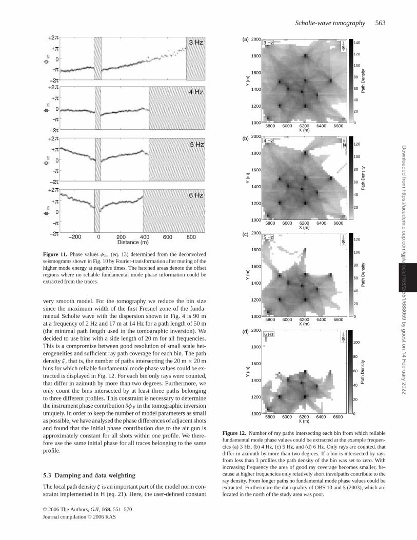
The hatched areas in Fig. 11 denote the offset regions where no re-liable fundamental mode phase information could be extracted fromthe traces. These areas include the very small offsets (smaller 50 m)due to the increasing influence of positioning errors as the offsetdecreases, the superposition of higher mode energy, and near fieldeffects. Moreover at far offsets the phase deteriorates because of theloss of amplitude with increasing offset. This latter effect is alsoobserved in the local p–f spectra (Fig. 8). The maximum offset us-able to infer fundamental mode phase values depends on the signal-to-noise ratio as well as on the frequency. From profile 23 (2002)we could use traces with source-receiver distances up to 800 mat low frequencies (3 Hz) and up to 300 m at high frequencies(6 Hz). This leads to a different number of paths intersecting thebins for each frequency (Fig. 12) in the subsequent tomographicinversion.
5.2 Model parametrization
The background-slowness model was parametrized in bins witha side length of 40 m because this is sufficient to represent this
C© 2006 The Authors, GJI, 168, 551–570
Journal compilation C© 2006 RAS
Dow
nloaded from https://academ
ic.oup.com/gji/article/168/2/551/688059 by guest on 14 February 2022
Scholte-wave tomography 563
Figure 11. Phase values φ lm (eq. 13) determined from the deconvolvedseismograms shown in Fig. 10 by Fourier-transformation after muting of thehigher mode energy at negative times. The hatched areas denote the offsetregions where no reliable fundamental mode phase information could beextracted from the traces.
very smooth model. For the tomography we reduce the bin sizesince the maximum width of the first Fresnel zone of the funda-mental Scholte wave with the dispersion shown in Fig. 4 is 90 mat a frequency of 2 Hz and 17 m at 14 Hz for a path length of 50 m(the minimal path length used in the tomographic inversion). Wedecided to use bins with a side length of 20 m for all frequencies.This is a compromise between good resolution of small scale het-erogeneities and sufficient ray path coverage for each bin. The pathdensity ξ , that is, the number of paths intersecting the 20 m × 20 mbins for which reliable fundamental mode phase values could be ex-tracted is displayed in Fig. 12. For each bin only rays were counted,that differ in azimuth by more than two degrees. Furthermore, weonly count the bins intersected by at least three paths belongingto three different profiles. This constraint is necessary to determinethe instrument phase contribution δφ P in the tomographic inversionuniquely. In order to keep the number of model parameters as smallas possible, we have analysed the phase differences of adjacent shotsand found that the initial phase contribution due to the air gun isapproximately constant for all shots within one profile. We there-fore use the same initial phase for all traces belonging to the sameprofile.
5.3 Damping and data weighting
The local path density ξ is an important part of the model norm con-straint implemented in H (eq. 21). Here, the user-defined constant
X (m)
Y (
m)
5800 6000 6200 6400 66001000
1200
1400
1600
1800
2000
Pat
h D
ensi
ty
0
20
40
60
80
100
120
140
X (m)
Y (
m)
5800 6000 6200 6400 66001000
1200
1400
1600
1800
2000
Pat
h D
ensi
ty
20
40
60
80
100
120
X (m)
Y (
m)
5800 6000 6200 6400 66001000
1200
1400
1600
1800
2000
Pat
h D
ensi
ty
0
20
40
60
80
100
120
X (m)
Y (
m)
5800 6000 6200 6400 66001000
1200
1400
1600
1800
2000
Pat
h D
ensi
ty
0
20
40
60
80
100
(a)
(b)
(c)
(d)
N
N
N
N
4 Hz
5 Hz
6 Hz
3 Hz
Figure 12. Number of ray paths intersecting each bin from which reliablefundamental mode phase values could be extracted at the example frequen-cies (a) 3 Hz, (b) 4 Hz, (c) 5 Hz, and (d) 6 Hz. Only rays are counted, thatdiffer in azimuth by more than two degrees. If a bin is intersected by raysfrom less than 3 profiles the path density of the bin was set to zero. Withincreasing frequency the area of good ray coverage becomes smaller, be-cause at higher frequencies only relatively short travelpaths contribute to theray density. From longer paths no fundamental mode phase values could beextracted. Furthermore the data quality of OBS 10 and 5 (2003), which arelocated in the north of the study area was poor.
C© 2006 The Authors, GJI, 168, 551–570
Journal compilation C© 2006 RAS
Dow
nloaded from https://academ
ic.oup.com/gji/article/168/2/551/688059 by guest on 14 February 2022
564 S. Kugler et al.
λ controls the strength of damping towards the background modeldepending on the path density. We use λ = 0.08 so if ξ is greaterthan about 30 paths, the resulting effective model-norm dampingfor this bin is less than 0.1β, with β being the damping parameterfor the bins that have not been intersected at all.
To find an appropriate combination of the damping parameters α,β and γ we first apply the tomographic inversion to synthetic datasets. Therefore, we calculate a synthetic data set for a constant phase-slowness residual model (δ p(r) = 1 s km−1 for all r). For instrumentphase contributions δφP random values from a normal distributionwith mean zero and variance one were used. We then determine thesynthetic data set dsynth by multiplying the design matrix G of thesource-receiver combinations of the 4-Hz field data (path density inFig. 12b) to this model vector. High amount of random noise wasthen added to the synthetic data set
dsynthi = dsynth
i + dsynth
10n, i = 1, . . . , N (26)
with dsynth = ∑Ni=1 |dsynth
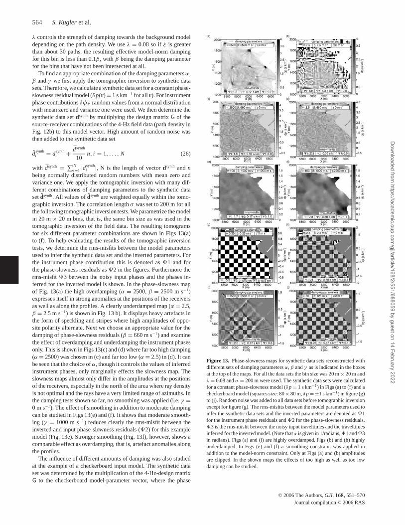
i |, N is the length of vector dsynth and nbeing normally distributed random numbers with mean zero andvariance one. We apply the tomographic inversion with many dif-ferent combinations of damping parameters to the synthetic dataset dsynth. All values of dsynth are weighted equally within the tomo-graphic inversion. The correlation length σ was set to 200 m for allthe following tomographic inversion tests. We parametrize the modelin 20 m × 20 m bins, that is, the same bin size as was used in thetomographic inversion of the field data. The resulting tomogramsfor six different parameter combinations are shown in Figs 13(a)to (f). To help evaluating the results of the tomographic inversiontests, we determine the rms-misfits between the model parametersused to infer the synthetic data set and the inverted parameters. Forthe instrument phase contribution this is denoted as �1 and forthe phase-slowness residuals as �2 in the figures. Furthermore therms-misfit �3 between the noisy input phases and the phases in-ferred for the inverted model is shown. In the phase-slowness mapof Fig. 13(a) the high overdamping (α = 2500, β = 2500 m s−1)expresses itself in strong anomalies at the positions of the receiversas well as along the profiles. A clearly underdamped map (α = 2.5,β = 2.5 m s−1) is shown in Fig. 13 b). It displays heavy artefacts inthe form of speckling and stripes where high amplitudes of oppo-site polarity alternate. Next we choose an appropriate value for thedamping of phase-slowness residuals (β = 660 m s−1) and examinethe effect of overdamping and underdamping the instrument phasesonly. This is shown in Figs 13(c) and (d) where far too high damping(α = 2500) was chosen in (c) and far too low (α = 2.5) in (d). It canbe seen that the choice of α, though it controls the values of inferredinstrument phases, only marginally effects the slowness map. Theslowness maps almost only differ in the amplitudes at the positionsof the receivers, especially in the north of the area where ray densityis not optimal and the rays have a very limited range of azimuths. Inthe damping tests shown so far, no smoothing was applied (i.e. γ =0 m s−1). The effect of smoothing in addition to moderate dampingcan be studied in Figs 13(e) and (f). It shows that moderate smooth-ing (γ = 1000 m s−1) reduces clearly the rms-misfit between theinverted and input phase-slowness residuals (�2) for this examplemodel (Fig. 13e). Stronger smoothing (Fig. 13f), however, shows acomparable effect as overdamping, that is, artefact anomalies alongthe profiles.
The influence of different amounts of damping was also studiedat the example of a checkerboard input model. The synthetic dataset was determined by the multiplication of the 4-Hz-design matrixG to the checkerboard model-parameter vector, where the phase
Figure 13. Phase-slowness maps for synthetic data sets reconstructed withdifferent sets of damping parameters α, β and γ as is indicated in the boxesat the top of the maps. For all the data sets the bin size was 20 m × 20 m andλ = 0.08 and σ = 200 m were used. The synthetic data sets were calculatedfor a constant phase-slowness model (δ p = 1 s km−1) in Figs (a) to (f) and acheckerboard model (squares size: 80 × 80 m, δ p = ±1 s km−1) in figure (g)to (j). Random noise was added to all data sets before tomographic inversionexcept for figure (g). The rms-misfits between the model parameters used toinfer the synthetic data sets and the inverted parameters are denoted as �1for the instrument phase residuals and �2 for the phase-slowness residuals.�3 is the rms-misfit between the noisy input traveltimes and the traveltimesinferred for the inverted model. (Note that α is given in 1/radians, �1 and �3in radians). Figs (a) and (i) are highly overdamped, Figs (b) and (h) highlyunderdamped. In Figs (e) and (f) a smoothing constraint was applied inaddition to the model-norm constraint. Only at Figs (a) and (b) amplitudesare clipped. In the shown maps the effects of too high as well as too lowdamping can be studied.
C© 2006 The Authors, GJI, 168, 551–570
Journal compilation C© 2006 RAS
Dow
nloaded from https://academ
ic.oup.com/gji/article/168/2/551/688059 by guest on 14 February 2022
Scholte-wave tomography 565
slowness of the model alternate between −1 and 1 s km−1 for 80 ×80 m bins. We still parametrize the model with 20 × 20 m bins.For a noise-free synthetic input data set the model can be perfectlyreconstructed (Fig. 13g). If we add random noise to the input dataset as is described in eq. (26) the effects of underdamping (Fig. 13h)and overdamping (Fig. 13i) are equivalent to the constant phase-slowness residual model. Additionally it can be seen that in areaswith excellent path coverage (around the coordinates X = 6300 mand Y = 1350 m) the model can be quite well reconstructed in spiteof the wrong choice of damping parameters. The inverted map foran appropriate set of damping parameters is shown in Fig. 13(j).
Based on the knowledge gained from these synthetic tests, wechoose the optimal set of damping parameters for the field data inthe following way. We begin with very small damping parameters α
and β and no smoothing (γ = 0 m s−1). Then we slowly increase α
until the artefacts of underdamping as shown in Fig. 13(b) disappear.So far we have still strong anomalies at the positions of the receivers.Now we increase β until the phase-slowness residuals at the posi-tions of the receivers are as close as possible to the residuals of thesurrounding. It wasn’t possible to totally eliminate those anomaliesin this way, but as we have learned from the synthetic tests these onlyfalsify the resulting model parameters of instrument phase contri-bution and phase-slowness residual at the positions of the receivers,leaving the rest of the model unchanged. Finally we slowly increasethe smoothing parameter γ but stop before the effects of overdamp-ing become apparent. The inferred damping parameter set for thefield data is α = 0.15, β = 140 m s−1 and γ = 250 m s−1. These aredifferent to the damping parameters used for the synthetic test datasets in Fig. 13 due to the different noise condition of the field data.The correlation length σ of the smoothing was set to 200 m. Wedecided to use the same parameter set for the tomographic inversionof all frequencies because we want to keep the model amplitudes fordifferent frequencies comparable since we need to infer dispersioncurves from the phase-slowness maps.
The weighting of the input data is implemented by the matrix Ce
in the objective function (17). Here, we want to weight reliable phasevalues more than biased values. To achieve this we incorporate thatthe difference between the residual phases of two adjacent pathswithin one profile is small. Therefore, we fit a polynomial of degree5 to the residual phases of each profile. We assume that the accurate,noise free phase values lie close to this polynomial, so we weight ourinput phases the more, the smaller the distance to this polynomialis.
6 R E S U LT S
6.1 Phase-slowness maps
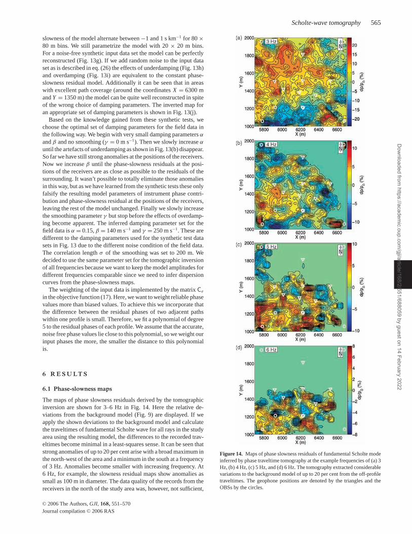
The maps of phase slowness residuals derived by the tomographicinversion are shown for 3–6 Hz in Fig. 14. Here the relative de-viations from the background model (Fig. 9) are displayed. If weapply the shown deviations to the background model and calculatethe traveltimes of fundamental Scholte wave for all rays in the studyarea using the resulting model, the differences to the recorded trav-eltimes become minimal in a least-squares sense. It can be seen thatstrong anomalies of up to 20 per cent arise with a broad maximum inthe north-west of the area and a minimum in the south at a frequencyof 3 Hz. Anomalies become smaller with increasing frequency. At6 Hz, for example, the slowness residual maps show anomalies assmall as 100 m in diameter. The data quality of the records from thereceivers in the north of the study area was, however, not sufficient,
Figure 14. Maps of phase slowness residuals of fundamental Scholte modeinferred by phase traveltime tomography at the example frequencies of (a) 3Hz, (b) 4 Hz, (c) 5 Hz, and (d) 6 Hz. The tomography extracted considerablevariations to the background model of up to 20 per cent from the off-profiletraveltimes. The geophone positions are denoted by the triangles and theOBSs by the circles.
C© 2006 The Authors, GJI, 168, 551–570
Journal compilation C© 2006 RAS
Dow
nloaded from https://academ
ic.oup.com/gji/article/168/2/551/688059 by guest on 14 February 2022
566 S. Kugler et al.
so that at high frequencies the paths were only in the southern halfof the area dense enough to extract information about the structuralslowness. In the northern part the slowness was damped to the back-ground model. Thus, the absence of anomalies in the northern part iscaused by a lack of information from the data and has no geologicalreason.
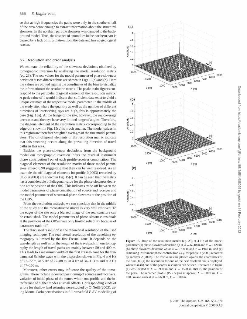
6.2 Resolution and error analysis
We estimate the reliability of the slowness deviations obtained bytomographic inversion by analysing the model resolution matrix(eq. 23). The row values for the model parameter of phase-slownessdeviation at two different bins are shown in Figs 15(a) and (b). Herethe values are plotted against the coordinates of the bins to visualizethe information of the resolution matrix. The peaks in the figures cor-respond to the particular diagonal element of the resolution matrix.A peak value of 1 would indicate that sufficient data exist to yield aunique estimate of the respective model parameter. In the middle ofthe study site, where the quantity as well as the number of differentdirections of intersecting rays are high, this is approximately thecase (Fig. 15a). At the fringe of the site, however, the ray coveragedecreases and the rays have very limited range of angles. Therefore,the diagonal element of the resolution matrix corresponding to theedge-bin shown in Fig. 15(b) is much smaller. The model values inthis region are therefore weighted averages of the true model param-eters. The off-diagonal elements of the resolution matrix indicatethat this smearing occurs along the prevailing direction of travelpaths in this area.
Besides the phase-slowness deviations from the backgroundmodel our tomographic inversion infers the residual instrumentphase contribution δφ P of each profile-receiver combination. Thediagonal elements of the resolution matrix of those model param-eters exceed 0.98 suggesting that they can be well resolved. As anexample the off-diagonal elements for profile 2(2003) recorded byOBS 2(2003) are shown in Fig. 15(c). It can be seen that the matrixhas a considerable off-diagonal value for the phase-slowness devia-tion at the position of the OBS. This indicates trade-off between themodel parameters of phase contribution of source and receiver andthe model parameter of structural phase slowness at the position ofthe OBS.
From the resolution analysis, we can conclude that in the middleof the study site the reconstructed model is very well resolved. Tothe edges of the site only a blurred image of the real structure canbe established. The model parameters of phase slowness residualsat the positions of the OBSs have only limited reliability because ofparameter trade-off.
The discussed resolution is the theoretical resolution of the usedimaging technique. The real lateral resolution of the traveltime to-mography is limited by the first Fresnel-zone. It depends on thewavelength as well as on the length of the travelpath. In our tomog-raphy the length of travel paths are mainly between 50 and 400 m.This leads to a maximum width of the first Fresnel-zone for the fun-damental Scholte wave with the dispersion shown in Fig. 4 at 6 Hzof 22–72 m, at 5 Hz of 27–88 m, at 4 Hz of 34–113 m and at 3 Hzof 47–156 m.
Moreover, other errors may influence the quality of the tomo-grams. These include incorrect positioning of sources and receivers,variation of initial phase of the source within one profile, and the in-terference of higher modes at small offsets. Corresponding kinds oferrors for shallow land seismics were studied by O’Neill (2003), us-ing Monte-Carlo perturbations in full wavefield P-SV modelling of
56005800
60006200
64006600
6800
1000
1500
2000
0
0.2
0.4
0.6
0.8
1
X (m)Y (m)
Am
plitu
de
56005800
60006200
64006600
6800
1000
1500
2000
0
0.2
0.4
0.6
0.8
1
X (m)Y (m)
Am
plit
ude
56005800
60006200
64006600
6800
1000
1500
2000
0
0.2
0.4
0.6
0.8
1
X (m)Y (m)
Am
plitu
de
(b)
(c)
(a)
N
N
N
Figure 15. Row of the resolution matrix (eq. 23) at 4 Hz of the modelparameter (a) phase-slowness deviation δp at X = 6240 m and Y = 1420 m,(b) phase-slowness deviation δp at X = 5700 m and Y = 1940 m, and (c)remaining instrument phase contribution δφ P for profile 2 (2003) recordedby receiver 2 (2003). The row values are plotted against the coordinates ofthe bins. In (a) the resolution for one of the best resolved bin is displayed,whereas in (b) one of the poorest resolution can be seen. Receiver 2 in figure(c) was located at X = 5900 m and Y = 1500 m, that is, the position ofthe peak. The recorded profile (P2) begins at approx. X = 6000 m, Y =1000 m and ends at X = 6600 m, Y = 1600 m.
C© 2006 The Authors, GJI, 168, 551–570
Journal compilation C© 2006 RAS
Dow
nloaded from https://academ
ic.oup.com/gji/article/168/2/551/688059 by guest on 14 February 2022
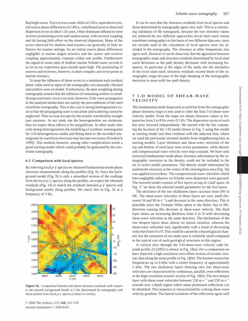
Scholte-wave tomography 567
Rayleigh waves. Trace to trace static shifts in CSGs, equivalent to ini-tial source phase differences in CRGs, contributed most to observeddispersion errors in ideal 1-D cases. Other dominant influences werereceiver positioning errors and random noise, with receiver couplingand tilt having little effect on the observed dispersion. Many of theerrors observed for shallow land seismics are generally of little in-fluence for marine settings. So are initial source phase differencesnegligible in marine airgun seismics and the source and receivercoupling approximately constant within one profile. Furthermorethe signal-to-noise ratio of shallow marine Scholte-wave records isas far as our experience goes mostly quite high. The positioning ofsources and receivers, however, is more complex and error-prone inmarine seismics.
To keep the influence of those errors to a minimum each residualphase value used as input of the tomography was manually checkedand outliers were excluded. Furthermore, the data weighting duringtomography assures that the influence of remaining outliers is small.Strong systematic errors can exist, however, if the wave propagationin the analysed media does not satisfy the preconditions of the usedtraveltime tomography. This is the case if strong heterogeneities ex-ist so that the propagating wave is not plane and scattering cannot beneglected. Then we may not specify the seismic wavefield by straightrays anymore. At our study site the heterogeneities are moderate,thus we expect these effects to be insignificant. At other study siteswith strong heterogeneities the modelling of synthetic seismogramsfor 3-D heterogeneous media and fitting them to the recorded seis-mograms by waveform inversion may become necessary (Friederich1999). This method, however, among other complications needs agood starting model which could probably be generated by the trav-eltime tomography.
6.3 Comparison with local spectra
By inferring local p–f spectra we obtained fundamental-mode phaseslowness measurements along the profiles (Fig. 9). Since the back-ground model (Fig. 9) is only a smoothed version of the readingsfrom the local p–f spectra along the profiles, we expect the obtainedresiduals (Fig. 14) to match the residuals between p–f spectra andbackground model along profiles. We check this in Fig. 16 at afrequency of 3 Hz.
X (m)
Y (
m)
5800 6000 6200 6400 66001000
1100
1200
1300
1400
1500
1600
1700
1800
1900
2000
dp/p
0 (%
)0
5
10
15
20
N
Figure 16. Comparison between the phase slowness residuals with respectto the smooth background model at 3 Hz determined by tomography andthose picked from local p–f spectra (values in circles).
It can be seen that the slowness residuals from local spectra andthose determined by tomography agree very well. This is a convinc-ing validation of the tomograms, because the two slowness valuesare achieved by two different approaches (local slant stack versustraveltime tomography) on the basis of two different data sets, sincethe records used in the calculation of local spectra were not in-cluded in the tomography. The slowness at other frequencies alsoagree well. However it can be observed, that the agreement betweentomographic maps and slowness residuals determined by local slantstack decreases as the path density decreases with increasing fre-quency. In particular at the edges of the study site the anomaliesof the local slant-stack slowness residuals exceed those of the to-mographic maps because of the high damping of the tomographicinversion in areas with low path density.
7 3 - D M O D E L O F S H E A R - WAV EV E L O C I T Y
The fundamental mode dispersion at each bin from the tomographicphase slowness maps is now used to infer the final 3-D shear-wavevelocity model. From the maps we obtain slowness values at fre-quencies from 2 to 8 Hz every 0.5 Hz. The dispersion curves of eachbin were inverted independently. We started with the bin contain-ing the location of the 1-D model shown in Fig. 5 using this modelas starting model and then continue with the adjacent bins, wherewe used the previously inverted models from neighbouring bins asstarting models. Layer thickness and shear-wave velocities of thetop and bottom of each layer were active parameters, while densityand compressional-wave velocity were kept constant. We have onlyextracted fundamental mode phase slowness information by the to-mographic inversion so the density could not be included in theset of active model parameters. The density model determined bymultimode inversion at the centre of the investigation area (Fig. 5b)was applied everywhere. The compressional-wave velocities whichhave negligible influence on Scholte wave dispersion were guessed.The inverted model consists of five layers on top of a half space. InFig. 17 we show the inferred model parameters for the five layers.
The thickness of the two shallowest layers increase from SW toNE. The shear-wave velocities of those layers are very small (be-tween 54 and 90 m s−1) and decrease in the same direction. This isplausible since the Tromper Wiek opens to the Baltic Sea in NE-direction causing this decrease in shear-wave velocity. The thirdlayer shows an increasing thickness from S to N with decreasingshear-wave velocities in the same direction. The thicknesses of thetwo deepest layers show almost no lateral variation, whereas theshear-wave velocities vary significantly with a trend of decreasingvelocities from S to N. This could be caused by a buried glacial chan-nel, but the extension of our study area is relatively small comparedto the typical size of such geological structures in this region.
A vertical slice through the 3-D-shear-wave velocity cube be-neath profile 23 (2002) is shown in Fig. 18(a). For a comparison wehave depicted a high-resolution zero-offset section of boomer seis-mic data along the same profile in Fig. 18(b). The boomer source hasfrequencies up to 6 kHz with a centre frequency of approximately2 kHz. The two shallowest layers showing very low shear-wavevelocities are characterized by continuous, parallel, even reflectionsin the high-resolution seismic section of Fig. 18(b). The next deeperlayer with shear-wave velocities between 150 m s−1 and 250 m s−1
extends over a depth region where many prominent reflections canbe identified. This sequence is characterized by a strong shear-wavevelocity gradient. The lateral variations of the reflections agree well
C© 2006 The Authors, GJI, 168, 551–570
Journal compilation C© 2006 RAS
Dow
nloaded from https://academ
ic.oup.com/gji/article/168/2/551/688059 by guest on 14 February 2022
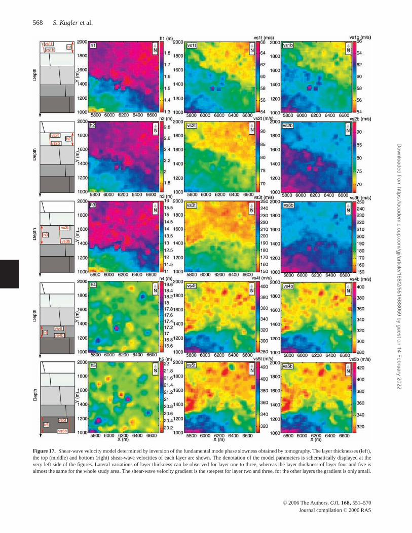
568 S. Kugler et al.
Figure 17. Shear-wave velocity model determined by inversion of the fundamental mode phase slowness obtained by tomography. The layer thicknesses (left),the top (middle) and bottom (right) shear-wave velocities of each layer are shown. The denotation of the model parameters is schematically displayed at thevery left side of the figures. Lateral variations of layer thickness can be observed for layer one to three, whereas the layer thickness of layer four and five isalmost the same for the whole study area. The shear-wave velocity gradient is the steepest for layer two and three, for the other layers the gradient is only small.
C© 2006 The Authors, GJI, 168, 551–570
Journal compilation C© 2006 RAS
Dow
nloaded from https://academ
ic.oup.com/gji/article/168/2/551/688059 by guest on 14 February 2022
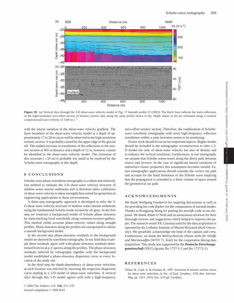
Scholte-wave tomography 569
Figure 18. (a) Vertical slice through the 3-D shear-wave velocity model of Fig. 17 beneath profile 23 (2002). The black lines indicate the main reflectionsof the high-resolution zero-offset section of boomer seismic data along the same profile shown in (b). Depth values in (b) are estimated using a constantcompressional-wave velocity of 1500 m s−1.
with the lateral variation of the shear-wave velocity gradient. Thelayer boundary of the shear-wave velocity model at a depth of ap-proximately 17 to 20 m can as well be observed in the high resolutionseismic section. It is probably caused by the upper edge of the glacialtill. The sudden increase in traveltimes of the reflections in the seis-mic section at 965 m distance and a depth of 12 m, however, cannotbe identified in the shear-wave velocity model. The extension ofthis structure (<50 m) is probably too small to be resolved by theScholte-wave tomography at this depth.
8 C O N C L U S I O N S
Scholte-wave phase-traveltime tomography is a robust and relativelyfast method to estimate the 3-D shear-wave velocity structure ofshallow-water marine sediments and is therefore (after calibrationof shear-wave velocity to shear strength) best suited for geotechnicalengineering applications in those environments.
A three-step tomographic approach is developed to infer the 3-D shear-wave velocity structure of shallow-water marine sedimentsusing the fundamental Scholte mode excited by air guns. In the firststep we construct a background model of Scholte phase slownessby slant-stacking local wavefields along common-receiver-gathers.This method yields accurate phase-velocity values along straightprofiles. Phase slowness along the profiles are extrapolated to obtaina smooth background model.
In the second step phase-slowness residuals to the backgroundmodel are derived by traveltime tomography. In our field data exam-ple these residuals agree well with phase-slowness residuals deter-mined from local p–f spectra along the profiles. The phase-slownessresiduals inferred by tomography together with the backgroundmodel established a phase-slowness dispersion curve at every lo-cation of the study site.
In the third step the depth-dependency of shear-wave velocitiesat each location was inferred by inverting the respective dispersioncurve leading to a 3-D model of shear-wave velocities. A verticalslice through this 3-D model agrees well with a high-frequency
zero-offset seismic section. Therefore, the combination of Scholte-wave traveltime tomography with areal high-frequency reflectiontraveltimes within a joint inversion seems to be promising.
Future work should focus on two important aspects. Higher modesshould be included in the tomographic reconstruction to infer a 3-D model not only of shear-wave velocity but also of density andto enhance the vertical resolution. Furthermore, in our tomographywe assume that Scholte waves travel along the direct path betweensource and receiver. In the case of significant lateral variations ofsubsurface elastic properties this assumption becomes invalid. Fu-ture tomographic applications should consider the correct ray pathand account for the band limitation of the Scholte wave implyingthat the propagation is extended to a finite volume of space aroundthe geometrical ray path.
A C K N O W L E D G M E N T S
We thank Wolfgang Friederich for inspiring discussions as well asfor providing his code flspher for the computation of normal modes.Thanks to Rongjiang Wang for putting his mseisfk-code at our dis-posal. We thank Adam O’Neill and an anonymous reviewer for theirthorough reviews and suggestions which helped to improve the pa-per. The research vessel FK Littorina used for the data acquisition isoperated by the Leibnitz-Institute of Marine Research (Kiel Univer-sity). We greatfully acknowledge the help of the captain and crew.Furthermore, we thank the Wehrtechnische Dienst stelle fur Schiffeund Marinewaffen (WTD 71, Kiel) for the cooperation during dataacquisition. This study was supported by the Deutsche Forschungs-gemeinschaft (DFG) (grants Bo 1727/1-2 and Bo 1727/2-1).
R E F E R E N C E S
Allnor, R., Caiti, A. & Arntsen, B., 1997. Inversion of seismic surface wavesfor shear wave velocities, in Soc. of Expl. Geophys., 67th Ann. Internat.Mtg, pp. 1921–1924, Soc. of Expl. Geophys.
C© 2006 The Authors, GJI, 168, 551–570
Journal compilation C© 2006 RAS
Dow
nloaded from https://academ
ic.oup.com/gji/article/168/2/551/688059 by guest on 14 February 2022
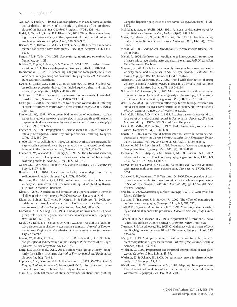
570 S. Kugler et al.
Ayres, A. & Theilen, F., 1999. Relationship between P- and S-wave velocitiesand geological properties of near-surface sediments of the continentalslope of the Barents Sea, Geophys. Prospect., 47(04), 431–441.
Badal, J., Dutta, U., Seron, F. & Biswas, N., 2004. Three-dimensional imag-ing of shear wave velocity in the uppermost 30 m of the soil column inAnchorage, Alaska, Geophys. J. Int., 158, 983–997.
Barmin, M.P., Ritzwoller, M.H. & Levshin, A.L., 2001. A fast and reliablemethod for surface wave tomography, Pure appl. geophys., 158, 1351–1375.
Boggs, P.T. & Tolle, J.W., 1995. Sequential quadratic programming, ActaNumerica, pp. 1–51.
Bohlen, T., Kugler, S., Klein, G. & Theilen, F., 2004. 1.5D inversion of lateralvariation of Scholte-wave dispersion, Geophysics, 69(02), 330–344.
Dombrowski, B., 1996. 3D-modeling, analysis and tomography of surfacewave data for engineering and environmental purposes, PhD Dissertation,Ruhr Universitat Bochum.
Ewing, J., Carter, J.A., Sutton, G.-H. & Barstow, N., 1992. Shallow wa-ter sediment properties derived from high-frequency shear and interfacewaves, J. geophys. Res., 97(B4), 4739–4762.
Forbriger, T., 2003a. Inversion of shallow-seismic wavefields: I. wavefieldtransformation, Geophys. J. Int., 153(3), 719–734.
Forbriger, T., 2003b. Inversion of shallow-seismic wavefields: II. Inferringsubsurface properties from wavefield transforms, Geophys. J. Int., 153(3),735–752.
Friederich, W., 1998. Wave-theoretical inversion of teleseismic surfacewaves in a regional network: phase-velocity maps and three-dimensionalupper-mantle shear-wave-velocity model for southern Germany, Geophys.J. Int., 132(1), 203–225.
Friederich, W., 1999. Propagation of seismic shear and surface waves in alaterally heterogeneous mantle by multiple forward scattering, Geophys.J. Int., 136, 180–204.
Friederich, W. & Dalkolmo, J., 1995. Complete synthetic seismograms fora spherically symmetric earth by a numerical computation of the Green’sfunction in the frequency domain, Geophys. J. Int., 122, 537–550.
Friederich, W., Wielandt, E. & Stange, S., 1993. Multiple forward scatteringof surface waves: Comparison with an exact solution and born single-scattering methods, Geophys. J. Int., 112, 264–275.
Gaiser, J.E., 1996. Multicomponent Vp/Vs correlation analysis, Geophysics,61(04), 1137–1149.
Hamilton, E.L., 1976. Shear-wave velocity versus depth in marinesediments—A review, Geophysics, 41(05), 985–996.
Herrmann, R. & Al-Eqabi, G., 1991. Surface wave inversion for shear wavevelocity, in Shear waves in marine sediments, pp. 545–556, ed. by Hovem,J., Kluwer Academic Publishers.
Klein, G., 2003. Acquisition and inversion of dispersive seismic waves inshallow marine environments, PhD Dissertation, Universitat Kiel.
Klein, G., Bohlen, T., Theilen, F., Kugler, S. & Forbriger, T., 2005. Ac-quisition and inversion of dispersive seismic waves in shallow marineenvironments, Marine Geophysical Researches, 2–4, 287–315.
Kocaoglu, A.H. & Long, L.T., 1993. Tomographic inversion of Rg wavegroup velocities for regional near-surface velocity structure, J. geophys.Res., 98(B4), 6579–6587.
Kugler, S., Bohlen, T., Bussat, S. & Klein, G., 2005. Variability of Scholte-wave dispersion in shallow-water marine sediments, Journal of Environ-mental and Engineering Geophysics, Special edition on surface waves,10(2), 203–218.
Lemke, W., Endler, R., Tauber, F., Jensen, J.B. & Bennike, O., 1998. Late-and postglacial sedimentation in the Tromper Wiek northeast of Rugen(western Baltic), Meyniana, 50, 155–173.
Long, L.T. & Kocaoglu, A.H., 2001. Surface-wave group-velocity tomog-raphy for shallow structures, Journal of Environmental and EngineeringGeophysics, 6(2), 71–81.
Lophaven, S.N., Nielsen, H.B. & Sondergaard, J., 2002. DACE-A MatlabKriging Toolbox, Version 2.0, Imm-rep-2002-12, Informatics and mathe-matical modelling, Technical University of Denmark.
Mari, J.L., 1984. Estimation of static corrections for shear-wave profiling
using the dispersion properties of Love-waves, Geophysics, 49(08), 1169–1179.
McMechan, G.A. & Yedlin, M.J., 1981. Analysis of dispersive waves bywave-field transformation, Geophysics, 46(06), 869–874.
Meier, T., Lebedev, S., Nolet, G. & Dahlen, F.A., 1997. Diffraction tomog-raphy using multimode surface waves, J. geophys. Res., 102(B4), 8255–8267.
Menke, W., 1989. Geophysical Data Analysis: Discrete Inverse Theory, Aca-demic Press.
Misiek, R., 1996. Surface waves: Application to lithostructural interpretationof near-surface layers in the meter and decameter range, PhD Dissertation,Ruhr Universitat Bochum.
Muyzert, E., 2000. Scholte wave velocity inversion for a near surface S-velocity model and P-S-statics, in Soc. of Expl. Geophys., 70th Ann. In-ternat. Mtg, pp. 1197–1200, Soc. of Expl. Geophys.
Nakanishi, I. & Anderson, D.L., 1982. World-wide distribution of groupvelocity of mantle Rayleigh waves as determined by spherical harmonicinversion, Bull. seism. Soc. Am., 72, 1185–1194.
Nakanishi, I. & Anderson, D.L., 1983. Measurements of mantle wave veloc-ities and inversion for lateral heterogeneity and anisotropy, 1. Analysis ofgreat circle phase velocities, J. geophys. Res., 88, 10 267–10 283.
O’Neill, A., 2003. Full-waveform reflectivity for modelling, inversion andappraisal of seismic surface wave dispersion in shallow site investigations,PhD Dissertation, University of Western Australia.
Park, C.B., Miller, R.D. & Xia, J., 1998. Imaging dispersion curves of sur-face waves on multi-channel record, in Soc. of Expl. Geophys., 68th Ann.Internat. Mtg, pp. 1377–1380, Soc. of Expl. Geophys.
Park, C.B., Miller, R.D. & Xia, J., 1999. Multichannel analysis of surfacewaves, Geophysics, 64(3), 800–808.
Rauch, D., 1986. On the role of bottom interface waves in ocean seismo-acoustics: a review, in Ocean Seismo-Acoustics Low Frequency Under-water Acoustics, Vol. 16, pp. 623–642, eds Akal, T. & Berkson, J.
Ritzwoller, M.H. & Levshin, A.L., 1998. Eurasian surface wave tomography:Group velocities, J. geophys. Res., 103(B3), 4839–4878.
Ritzwoller, M.H., Shapiro, N.M., Barmin, M.P. & Levshin, A.L., 2002.Global surface wave diffraction tomography, J. geophys. Res., 107(B12),2335, doi:10.1029/2002JB001777.
Ritzwoller, M.H. & Levshin, A.L., 2002. Estimating shallow shear velocitieswith marine multicomponent seismic data, Geo-physics, 67(06), 1991–2004.
Schalkwijk, K., Wapenaar, C. & Verschuur, D., 2000. Decomposition of mul-ticomponent ocean-bottom data: Inversion for the subbottom parameters,in Soc. of Expl. Geophys., 70th Ann. Internat. Mtg, pp. 1205–1208, Soc.of Expl. Geophys.
Snieder, R., 2002. Scattering of surface waves, pp. 562–577, Academic, SanDiego, California.
Spetzler, J., Trampert, J. & Snieder, R., 2002. The effect of scattering insurface wave tomography, Geophys. J. Int., 149, 755–767.
Stoll, R.D., Bryan, G.M. & Bautista, E.O., 1994. Measuring lateral variabil-ity of sediment geoacoustic properties, J. acoust. Soc. Am., 96(1), 427–438.
Tatham, R.H. & Goolsbee, D.V., 1984. Separation of S-wave and P-wavereflections offshore western Florida, Geophysics, 49(05), 493–508.
Trampert, J. & Woodhouse, J.H., 1995. Global phase velocity maps of Loveand Rayleigh waves between 40 and 150 seconds, Geophys. J. Int., 122,675–690.
Wang, R., 1999. A simple orthonormalization method for stable and effi-cient computations of green’s functions, Bulletin of the Seismic Society ofAmerica, 89(3), 733–741.
Wielandt, E., 1993. Propagation and structural interpretation of non-planewaves, Geophys. J. Int., 113(1), 45–53.
Wielandt, E. & Schenk, H., 1983. On systematic errors in phase-velocityanalysis, J. Geophys., 52, 1–6.
Woodhouse, J.H. & Dziewonski, A.M., 1984. Mapping the upper manlte:Threedimensional modeling of earth structure by inversion of seismicwaveforms, J. geophys. Res., 89, 5953–5986.
C© 2006 The Authors, GJI, 168, 551–570
Journal compilation C© 2006 RAS
Dow
nloaded from https://academ
ic.oup.com/gji/article/168/2/551/688059 by guest on 14 February 2022
Related Documents