SCHEMA MATCHING AND DATA EXTRACTION OVER HTML TABLES by Cui Tao A thesis submitted to the faculty of Brigham Young University in partial fulfillment of the requirements for the degree of Master of Science Department of Computer Science Brigham Young University September 8, 2003

Welcome message from author
This document is posted to help you gain knowledge. Please leave a comment to let me know what you think about it! Share it to your friends and learn new things together.
Transcript

SCHEMA MATCHING AND DATA EXTRACTION OVER HTML
TABLES
by
Cui Tao
A thesis submitted to the faculty of
Brigham Young University
in partial fulfillment of the requirements for the degree of
Master of Science
Department of Computer Science
Brigham Young University
September 8, 2003

Copyright c© 2003 Cui Tao
All Rights Reserved

BRIGHAM YOUNG UNIVERSITY
GRADUATE COMMITTEE APPROVAL
of a thesis submitted by
Cui Tao
This thesis has been read by each member of the following graduate committee and bymajority vote has been found to be satisfactory.
Date David W. Embley, Chair
Date Stephen W. Liddle
Date Thomas W. Sederberg
BRIGHAM YOUNG UNIVERSITY
As chair of the candidate’s graduate committee, I have read the thesis of Cui Tao in its finalform and have found that (1) its format, citations, and bibliographical style are consistentand acceptable and fulfill university and department style requirements; (2) its illustrativematerials including figures, tables, and charts are in place; and (3) the final manuscript issatisfactory to the graduate committee and is ready for submission to the university library.
Date David W. EmbleyChair, Graduate Committee
Accepted for the Department
David W. EmbleyGraduate Coordinator
Accepted for the College
G. Rex BryceAssociate DeanCollege of Physical and Mathematical Sciences

ABSTRACT
SCHEMA MATCHING AND DATA EXTRACTION OVER HTML TABLES
Cui Tao
Department of Computer Science
Master of Science
Data on the Web in HTML tables is mostly structured, but we usually do not know
the structure in advance. Thus, we cannot directly query for data of interest. We propose
a solution to this problem for the case of mostly structured data in the form of HTML ta-
bles, based on document-independent extraction ontologies. The solution entails elements
of table location and table understanding, data integration, and wrapper creation. Table
location and understanding allows us to locate the table of interest, recognize attributes and
values, pair attributes with values, and form records. Data-integration techniques allow us
to match source records with a target schema. Ontologically specified wrappers allow us to
extract data from source records into a target schema. Experimental results show that we
can successfully map data of interest from source HTML tables with unknown structure to
a given target database schema. We can thus “directly” query source data with unknown
structure through a known target schema.

ACKNOWLEDGMENTS
First of all, I would like to thank my advisor, Dr. David W. Embley. Under his
guidance, I successfully overcame many difficulties and learned a lot about how to be a
good researcher.
Secondly, I would like to thank my other committee members. I thank Dr. Stephen
W. Liddle for his unique insight into software implementation and his help in coding. I
thank Dr. Thomas W. Sederberg for his time and effort on my thesis.
I would like to thank my husband, Zonghui, for his continued love, patience, under-
standing and support during this project and my entire endeavor to become more educated.
I also want to thank my parents for teaching me how to learn and how to learn well and for
encouraging my interest in science since I was a little girl. I thank my sister, Wei and my
brother in law, Yue, for encouraging me and supporting my interest in Computer Science.
I thank the National Science Foundation for supporting this research under grant
#qS-0083127.
Last, but not least, I thank all the BYU data-extraction research group members for
their support and suggestions on my research.

Contents
Acknowledgments vi
List of Figures x
1 INTRODUCTION 1
1.1 Background and Related Work . . . . . . . . . . . . . . . . . . . . . . . . 1
1.2 HTML Table Problems . . . . . . . . . . . . . . . . . . . . . . . . . . . . 3
1.2.1 HTML Tables—Location Problems . . . . . . . . . . . . . . . . . 4
1.2.2 HTML Tables—Extraction Problems . . . . . . . . . . . . . . . . 6
2 EXTRACTION ONTOLOGIES 11
3 TABLE LOCATION AND UNDERSTANDING 15
3.1 Overview of HTML Tables . . . . . . . . . . . . . . . . . . . . . . . . . . 15
3.2 DOM Representation . . . . . . . . . . . . . . . . . . . . . . . . . . . . . 18
3.3 Table Location Heuristics . . . . . . . . . . . . . . . . . . . . . . . . . . . 19
3.3.1 Location – Top-Level Tables . . . . . . . . . . . . . . . . . . . . . 19
3.3.2 Location – Linked-Page Tables . . . . . . . . . . . . . . . . . . . . 21
3.4 Table Preprocessing and Understanding . . . . . . . . . . . . . . . . . . . 22
4 MAPPING INFERENCE 31
4.1 Generate and Adjust Attribute-Value Pairs . . . . . . . . . . . . . . . . . . 31
4.2 Infer Mapping . . . . . . . . . . . . . . . . . . . . . . . . . . . . . . . . . 33
4.2.1 Pattern Recognition . . . . . . . . . . . . . . . . . . . . . . . . . . 33
4.2.2 Mapping Inference . . . . . . . . . . . . . . . . . . . . . . . . . . 35
vii

5 EXPERIMENTAL ANALYSIS 41
5.1 Car Advertisements . . . . . . . . . . . . . . . . . . . . . . . . . . . . . . 41
5.1.1 Results—Car Advertisements . . . . . . . . . . . . . . . . . . . . 42
5.1.2 Cell-Phone Sales . . . . . . . . . . . . . . . . . . . . . . . . . . . 44
6 CONCLUSIONS AND FUTURE WORK 49
6.1 Conclusions . . . . . . . . . . . . . . . . . . . . . . . . . . . . . . . . . . 49
6.2 Future Work and Interesting Unresolved Table Problems . . . . . . . . . . 49
Bibliography 56
A INTERESTING UNRESOLVED TABLES 59
viii
List of Figures
1.1 Sample Tables for Target Schema . . . . . . . . . . . . . . . . . . . . . . . 3
1.2 Web Page with Table from www.bobhowardhonda.com [9] . . . . . . . . . 4
1.3 Linked Page with Additional Information [9] . . . . . . . . . . . . . . . . 5
1.4 Table from Autoscanada.com [5] . . . . . . . . . . . . . . . . . . . . . . . 5
2.1 Car-Ads Extraction Ontology (Partial) . . . . . . . . . . . . . . . . . . . . 12
3.1 An Example of an HTML Table . . . . . . . . . . . . . . . . . . . . . . . 17
3.2 DOM Tree of the Table in Figure 3.1 . . . . . . . . . . . . . . . . . . . . . 18
3.3 An Example of Folded Table in a Linked Page (www.jscars.com [35]) . . . 24
3.4 The Unfolded Table for the Table in Figure 3.3 . . . . . . . . . . . . . . . 24
3.5 An Example of an Internal Factor . . . . . . . . . . . . . . . . . . . . . . 25
3.6 The New Table with Years Distributed to the Value Rows for the Table in
Figure 3.5 . . . . . . . . . . . . . . . . . . . . . . . . . . . . . . . . . . . 26
3.7 An Example of Table Header (www.autobytel.com [3]) . . . . . . . . . . . 27
3.8 Top Table After Preprocess for the Table in Figure 1.2 . . . . . . . . . . . . 27
3.9 Extended Table of the Information in Figure 1.3 . . . . . . . . . . . . . . . 28
3.10 An Example Result Table for Single-Attribute Table . . . . . . . . . . . . . 29
4.1 A Table that has Boolean Values and the Table Transformed by theβ Operator 33
4.2 Data Frame for the Make Object Set in Car-Ads Extraction Ontology (Partial) 35
4.3 Columns Added to the Table in Figure 4.4 by theδ Operator . . . . . . . . 36
4.4 An Sample Source Table . . . . . . . . . . . . . . . . . . . . . . . . . . . 37
4.5 Extracted Result from the Table in Figure 4.4 . . . . . . . . . . . . . . . . 37
4.6 Application of theγ Operator to TableT1 Yielding TableT2 . . . . . . . . . 38
4.7 Inferred Mapping from Source TableT in Figure 4.1a to the Target Table
in Figure 4.8 . . . . . . . . . . . . . . . . . . . . . . . . . . . . . . . . . . 39
ix
4.8 Sample Tables for Target Schema . . . . . . . . . . . . . . . . . . . . . . . 39
4.9 Inferred Mapping from the Source TablesT in Figure 1.2,T ′ in Figure 3.9,
andT ′′ in Figure 3.10 and from P, the page in in Figure 1.2, to the Target
Table in Figure 4.8 . . . . . . . . . . . . . . . . . . . . . . . . . . . . . . 40
5.1 Web Page with Table of Cell Phones from Buy.com . . . . . . . . . . . . . 45
5.2 Linked Page with Additional Cell Phone Information from Buy.com . . . . 46
A.1 Table with Complicated Structure (Multiple Schemas and Long Factors) [51] 60
A.2 Table with Complicated Structure (Each Record Takes Multiple Rows) [6] . 61
A.3 Table with Complicated Schema (Attributes Take Multiple Rows) [46] . . . 61
A.4 Table with Image Attributes [12] . . . . . . . . . . . . . . . . . . . . . . . 62
A.5 Tables in Table [8] . . . . . . . . . . . . . . . . . . . . . . . . . . . . . . 62
A.6 Table with Irrelevant Images Inside [14] . . . . . . . . . . . . . . . . . . . 63
A.7 Each Record in the Top-Level Table Contains an Attribute-Value Table [1] . 64
A.8 Top-Level Table with Image Colors [13] . . . . . . . . . . . . . . . . . . . 65
A.9 View Detailed Information by Moving a Mouse [13] . . . . . . . . . . . . 66
A.10 Top-Level Table with Complicated Structure [16] . . . . . . . . . . . . . . 67
A.11 Top-Level Table with Only 2 Columns [4] . . . . . . . . . . . . . . . . . . 67
A.12 Top-Level Table with Complicated Structure [10] . . . . . . . . . . . . . . 68
A.13 Top-Level Table with Complicated Structure and Image [47] . . . . . . . . 68
A.14 Complicated Attribute-Value-Pair Table in a Linked Page [8] . . . . . . . . 69
A.15 Non-fixed Positions of Attribute and Value in Attribute-Value-Pair Table in
Linked Pages [44] . . . . . . . . . . . . . . . . . . . . . . . . . . . . . . . 70
A.16 List with Checked Marks [36] . . . . . . . . . . . . . . . . . . . . . . . . 70
x

Chapter 1
INTRODUCTION
1.1 Background and Related Work
Currently, with the fast development of the Internet, both the amount of useful data
and the number of sites on the World Wide Web (WWW) are growing rapidly. The Web is
becoming an increasingly useful information tool for computer users. However, there are
so many Web pages that no human being can traverse all of them to obtain the information
needed. A system that can allow users to query Web pages like a database is becoming
increasingly desirable.
The data-extraction research group at Brigham Young University (BYU) has de-
veloped an ontology-based querying approach, which can extract data from unstructured
Web documents [19]. Although this approach improved the automation of unstructured
data extraction, it does not work very well with mostly-structured data. Mostly-structured
WWW pages, such as Web pages containing HTML tables, are major barriers to BYU’s
automated ontology-based data extraction. About 52% of HTML documents include tables
[40]. Although some of these tables are only for physical layout, there is still a significant
amount of online data that is stored in HTML tables.
The solution to querying data whose sources are HTML tables encompasses ele-
ments of (1) table understanding, (2) data integration, and (3) information extraction [27].
Table understanding allows us to recognize attributes and values in a given table. It is a
complicated problem [31]. Most research to date uses low-level geometric information to
recognize tables [41]. Some of the current geometric modeling techniques for identify-
ing tabular structure use syntactic heuristics such as contiguous space between lines and
1
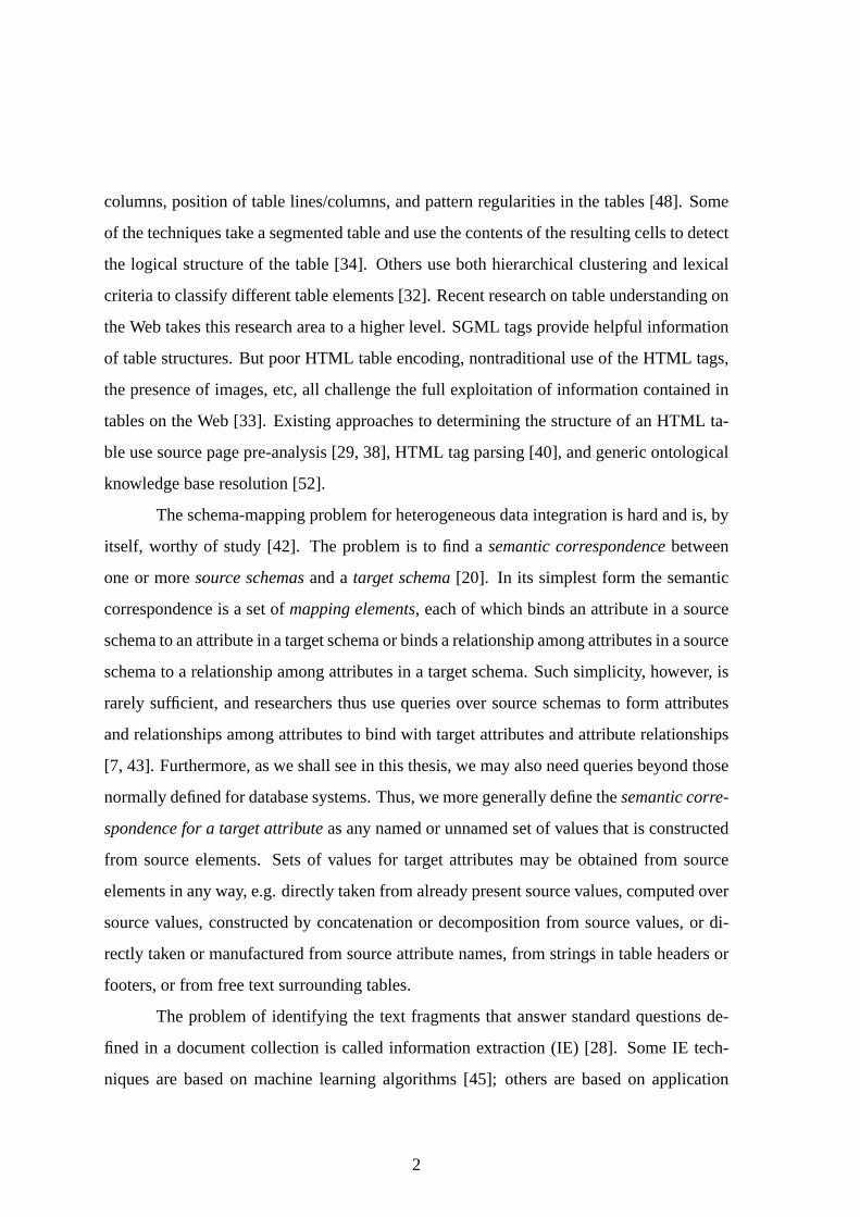
columns, position of table lines/columns, and pattern regularities in the tables [48]. Some
of the techniques take a segmented table and use the contents of the resulting cells to detect
the logical structure of the table [34]. Others use both hierarchical clustering and lexical
criteria to classify different table elements [32]. Recent research on table understanding on
the Web takes this research area to a higher level. SGML tags provide helpful information
of table structures. But poor HTML table encoding, nontraditional use of the HTML tags,
the presence of images, etc, all challenge the full exploitation of information contained in
tables on the Web [33]. Existing approaches to determining the structure of an HTML ta-
ble use source page pre-analysis [29, 38], HTML tag parsing [40], and generic ontological
knowledge base resolution [52].
The schema-mapping problem for heterogeneous data integration is hard and is, by
itself, worthy of study [42]. The problem is to find asemantic correspondencebetween
one or moresource schemasand atarget schema[20]. In its simplest form the semantic
correspondence is a set ofmapping elements, each of which binds an attribute in a source
schema to an attribute in a target schema or binds a relationship among attributes in a source
schema to a relationship among attributes in a target schema. Such simplicity, however, is
rarely sufficient, and researchers thus use queries over source schemas to form attributes
and relationships among attributes to bind with target attributes and attribute relationships
[7, 43]. Furthermore, as we shall see in this thesis, we may also need queries beyond those
normally defined for database systems. Thus, we more generally define thesemantic corre-
spondence for a target attributeas any named or unnamed set of values that is constructed
from source elements. Sets of values for target attributes may be obtained from source
elements in any way, e.g. directly taken from already present source values, computed over
source values, constructed by concatenation or decomposition from source values, or di-
rectly taken or manufactured from source attribute names, from strings in table headers or
footers, or from free text surrounding tables.
The problem of identifying the text fragments that answer standard questions de-
fined in a document collection is called information extraction (IE) [28]. Some IE tech-
niques are based on machine learning algorithms [45]; others are based on application
2

Car Year Make Model Mileage Price PhoneNr Car Feature0001 1999 Pontiac Firebird 32,833 405-936-8666 0001 Blue0002 2000 Acura RL 3.5 36,657 $23,988 405-936-8666 0001 ...0003 2002 Honda Accord EX 13.875 $21,988 405-936-8666 ... ...
... ...0003 White
0101 1992 ACURA legend $9500 0003 Air Conditioning0102 2000 AUDI A4 $34,500 0003 Driver Side Air Bag0103 1985 BMW 325e $2700.00 ...
0101 Auto0101 AM/FM
...
Figure 1.1: Sample Tables for Target Schema
ontologies [22, 23, 24]. In this thesis, we intend to use ontology-based extractors as an aid
to do element-level and instance-level schema matching.
1.2 HTML Table Problems
We limit our discussion here to HTML tables found on the Web.1 We consider
Web pages containing HTML tables of interest for a given application domain to be our
sources. We also include pages linked from within these HTML tables. Our target is a
simple relational schema.
As a running example, we use car advertisements, which are plentiful on the Web
and which often present their information in tables. Suppose, for example, that we are
interested in viewing and querying Web car ads through the target database in Figure 1.1,
whose schema is
{Car, Year, Make, Model, Mileage, Price, PhoneNr}{Car, Feature}.
Figures 1.2 [9], 1.3 [9], and 1.4 [5] show some potential source tables. The data in the
tables in Figure 1.1 is a small part of the data that can be extracted from Figures 1.2, 1.3,
and 1.4.1The problems encountered in HTML tables are more than sufficient for this investigation. Table extrac-
tion within the broader context of images of paper tables and other types of electronic tables [41] is alsopossible.
3
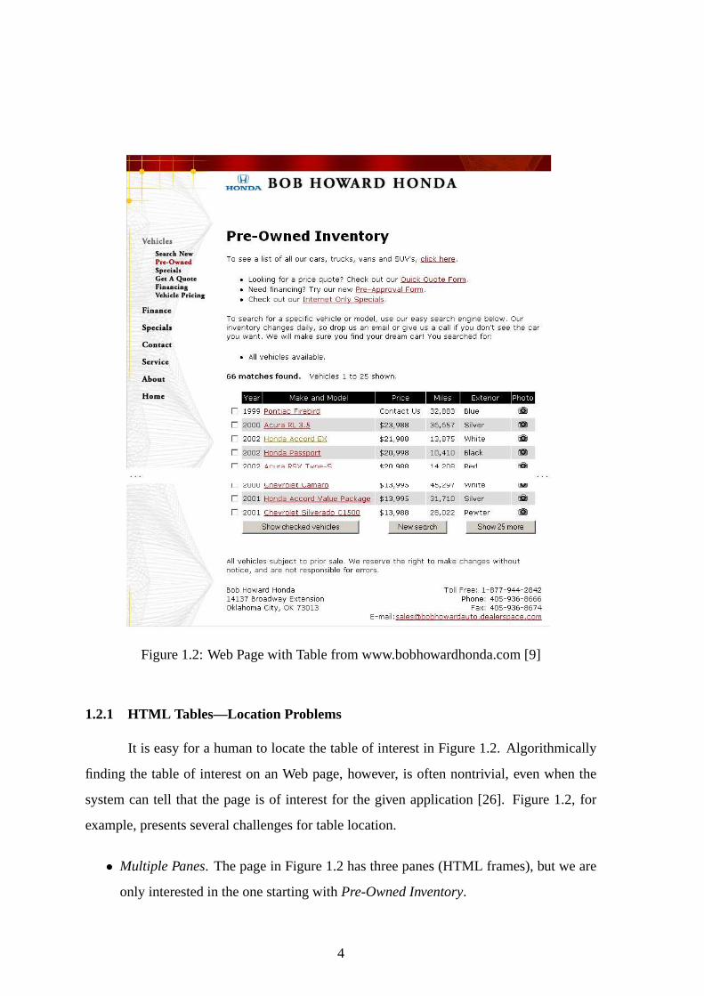
Figure 1.2: Web Page with Table from www.bobhowardhonda.com [9]
1.2.1 HTML Tables—Location Problems
It is easy for a human to locate the table of interest in Figure 1.2. Algorithmically
finding the table of interest on an Web page, however, is often nontrivial, even when the
system can tell that the page is of interest for the given application [26]. Figure 1.2, for
example, presents several challenges for table location.
• Multiple Panes. The page in Figure 1.2 has three panes (HTML frames), but we are
only interested in the one starting withPre-Owned Inventory.
4

Figure 1.3: Linked Page with Additional Information [9]
Figure 1.4: Table from Autoscanada.com [5]
5

• Tables for Layout. In the pane of interest in Figure 1.2, the first<TABLE> tag
encountered has two lines: the first for the text above the table, and the second for
the table and the footer text below the table.
• Table Rows Not in Table. The last two lines of the table in Figure 1.2 are not actually
part of the table. The last line contains the contact information, and the next-to-last
line contains the buttons and the claim of nonresponsibility.
• Tables Displayed Piecemeal. The table in Figure 1.2 displays 25 rows per page. To
obtain the rest of the table rows, we need to have the system simulate a click onShow
25 more.
• Tables Spanning Multiple Pages. We obtain the page in Figure 1.3 by clicking on
Honda Accord EXin the table in Figure 1.2. Clicking on all makes and models gives
us similar pages. Each page has a column of attribute-value pairs that starts with
Priceand ends withVIN. The collection of these columns from each page constitutes
a large table whose attributes are all the same,Price ... VIN, and whose values are
the value columns from each linked page.
• No <TABLE> Tag. Each linked page similar to the one in Figure 1.3 also has a
single-column table headed byFeatures. The source, however, does not tag this table
with a<TABLE> tag, but rather with a<UL> tag, making it an HTML list.
In general there are even more challenges for locating tables. We have listed here only the
challenges that appear in Figures 1.2 and 1.3. We list other challenges in the discussion of
future work in Chapter 6.
1.2.2 HTML Tables—Extraction Problems
Not only is it easy for a human to find the tables of interest in Figures 1.2 and 1.3,
it is also easy for a human to parse the table and determine its meaning. Even with the
constraint imposed of needing to match a source table with respect to a fixed target view,
such as the one in Figure 1.1, semantic matching is mostly straightforward for a human. It
is easy to see thatYearin the source table in Figure 1.2 as well asYearin the source table in
6

Figure 1.4 map toYearin the target table in Figure 1.1. It is also easy to see that although
Make andModel in Figure 1.4 match directly withMake andModel in Figure 1.1, we
need to splitMake and Modelin Figure 1.2 to matchMake andModel in Figure 1.1. It is
not as easy, however, to see that bothExterior in Figure 1.2 andColour in Figure 1.4 map
to Featurein Figure 1.1, and it is a little harder to see that we should map the attributes
Auto, Air Cond., AM/FM, andCD in Figure 1.4 as values forFeaturein Figure 1.1, but
only for “Yes” values.
Algorithmically sorting out these semantic matches is significantly harder. We en-
counter the following list of challenges when trying to match source HTML tables in Fig-
ures 1.2, 1.3, and 1.4 with the target schema in Figure 4.8. We list other challenges in the
discussion of our future work in Chapter 6.
• Merged Attributes/Values. MakeandModelare separate attributes in Figure 1.1 but
are merged as one attribute in Figure 1.2.
• Subsets. Exterior in Figure 1.2 andColour in Figure 1.4 contain colors. Colors in
the target are a special kind ofFeatureand thus the sets of colors in Figures 1.2 and
1.4 are subsets of the feature values we want for Figure 1.1. Indeed, these are proper
subsets since there are also many other feature values in Figures 1.2, 1.3, and 1.4.
• Synonyms. Mileage in Figure 1.1 andMiles in Figure 1.2 have the same meaning,
but the attribute names are not the same.
• Extra Information. The tables in Figure 1.1 make no request for photographs, which
are present in Figure 1.2.
• Linked Information. The values for the attributeMake and Modelare linked to further
information. Clicking onHonda Accord EXin Figure 1.2 yields the information in
Figure 1.3.
• List Table. A one-dimensional table and a list are similar in appearance.Featuresin
Figure 1.3 is a list, but could just as easily have been formatted as a table. Although
it is a list, we nevertheless wish to matchFeaturesin Figure 1.3 withFeature in
Figure 1.1.
7

• Position of Attributes. The linked subtable in Figure 1.3 has its attributes in the left
column, rather than in the top row.
• Missing Information. The schema in Figure 1.1 expects a phone number, but none of
the tables in Figures 1.2, 1.3, or 1.4 contains a phone number.
• Externally Factored Data. Although no phone number appears in the tables in Fig-
ures 1.2 or 1.3, phone numbers do appear in the footer text of the table in Figure 1.2
and in the text above the tables in Figure 1.3. A value, such as a dealer phone num-
ber, that applies to all records in a table is often factored out, external to the table,
and displayed only once.
• Duplicate Data. The price for theHonda Accord EXin Figures 1.2 and 1.3 appears
three times, once underPrice in Figure 1.2, once as the value for thePrice attribute
in the (vertical) table row in Figure 1.3, and once at the top of the layout table in
Figure 1.3. (Luckily, the values are all the same.) Other values also appear more than
once. The number of miles, in fact, appears with two different attributes, once with
Milesand once withMileage.
• Unexpected Multiple Values. The schema in Figure 1.1 expects at most one contact
phone number for each vehicle, but there may be several as Figures 1.2 and 1.3 show.
• Attribute as Value. In Figure 1.4, the featuresAuto, Air Cond., AM/FM, andCD are
all attributes rather than values. Here, we must understand thatYesandNo are not
the values; rather they indicate whether the valuesAuto, Air Cond., AM/FM, andCD
should be included asFeaturevalues in the tables in Figure 1.1.
In this thesis, we develop a system that can automatically locate the table of interest
in a Web page using a set of heuristics and our ontology technology, infer mappings from
source table attributes to the target schema, and extract information from source table(s) to
the target database.
The rest of this thesis in organized as follows: Chapter 2 introduces our ontology
based extraction technology. Chapter 3 discusses our approach to table location. Chapter 4
8

describes how the system infers mappings from source to target. Chapter 5 introduces and
analyzes experimental results. Chapter 6 discusses our conclusions and future work.
9

10
Chapter 2
EXTRACTION ONTOLOGIES
An extraction ontology is a conceptual-model instance that serves as a wrapper for a
narrow domain of interest such as car ads [22]. The conceptual-model instance includes ob-
jects, relationships, constraints over these objects and relationships, descriptions of strings
for lexical objects, and keywords denoting the presence of objects and relationships among
objects. When we apply an extraction ontology to a Web page, the ontology identifies the
objects and relationships and associates them with named object sets and relationship sets
in the ontology’s conceptual-model instance and thus wraps the recognized strings on a
page and makes them “understandable” in terms of the schema implicitly specified in the
conceptual-model instance. The hard part of writing a wrapper for extraction is to make it
robust so that it works for all sites, including sites not in existence at the time the wrapper is
written and sites that change their layout and content after the wrapper is written. Wrappers
based on extraction ontologies are robust.1 Robust wrappers are critical to our approach:
without them, we may have to create (by hand or at best semiautomatically) a wrapper for
every new table encountered; with them, the approach can be fully automatic.
1Page-specific, handwritten wrappers (e.g. the early wrappers produced for TSIMMIS [15]) are not ro-bust. Machine-learning-based wrappers (e.g. [37, 50]) are not robust since new and changed pages mustbe annotated and learned. Wrappers that automatically infer regular expressions for Web pages (e.g. [18])are robust in the sense that the regular-expression generator only needs to be rerun for new and changedpages; however, high page layout regularity is required, an assumption that often fails, but which we intendto consider in our future work with tables. Extraction ontologies (e.g. [22]) are robust because they arebased on conceptual-model specifications of a domain of interest, not on page layout. Although they arehand-crafted, as ontologies typically are, our experience shows that an expert can create a reasonably goodextraction ontology for a narrow domain of interest such as car ads in a few-dozen hours.
11
1. Car [-> object];2. Car [0:1] has Year [1:*];3. Car [0:1] has Make [1:*];4. Car [0:1] has Model [1:*];5. Car [0:1] has Mileage [1:*];6. Car [0:*] has Feature [1:*];7. Car [0:1] has Price [1:*];8. PhoneNr [1:*] is for Car [0:1];9. Year matches [4]
10. constant {extract " \d{2}";11. context " \b’[4-9] \d\b";12. substitute " ˆ" -> "19"; },13. ...14. Mileage matches [8]15. ...16. keyword " \bmiles \b", " \bmi \.", " \bmi \b",17. " \bmileage \b", " \bodometer \b";18. ...
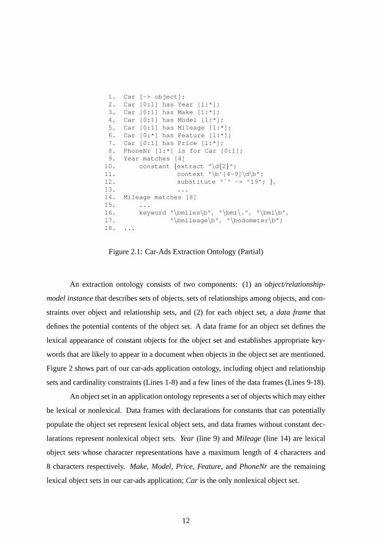
Figure 2.1: Car-Ads Extraction Ontology (Partial)
An extraction ontology consists of two components: (1) anobject/relationship-
model instancethat describes sets of objects, sets of relationships among objects, and con-
straints over object and relationship sets, and (2) for each object set, adata framethat
defines the potential contents of the object set. A data frame for an object set defines the
lexical appearance of constant objects for the object set and establishes appropriate key-
words that are likely to appear in a document when objects in the object set are mentioned.
Figure 2 shows part of our car-ads application ontology, including object and relationship
sets and cardinality constraints (Lines 1-8) and a few lines of the data frames (Lines 9-18).
An object set in an application ontology represents a set of objects which may either
be lexical or nonlexical. Data frames with declarations for constants that can potentially
populate the object set represent lexical object sets, and data frames without constant dec-
larations represent nonlexical object sets.Year (line 9) andMileage (line 14) are lexical
object sets whose character representations have a maximum length of 4 characters and
8 characters respectively.Make, Model, Price, Feature, andPhoneNrare the remaining
lexical object sets in our car-ads application;Car is the only nonlexical object set.
12

We describe the constant lexical objects and the keywords for an object set by reg-
ular expressions using Perl-like syntax.2 When applied to a textual document, theextract
clause (e.g. line 10) in a data frame causes a string matching a regular expression to be
extracted, but only if thecontext clause (e.g. line 11) also matches the string and its
surrounding characters. Asubstitute clause (e.g. line 12) lets us alter the extracted
string before we store it in an intermediate file. (For example, theYeardata frame treats
a year written “’95 ” as the constant “1995 ”.) We also store the string’s position in the
document and its associated object-set name in the intermediate file. One of the nonlexical
object sets must be designated as theobject set of interest—Car for the car-ads ontology,
as indicated by the notation “[-> object] ” in line 1.
We denote a relationship set by a name that includes its object-set names (e.g.Car
has Yearin line 2 andPhoneNr is for Carin line 8). Themin:maxpairs in the relationship-
set name areparticipation constraints. Min designates the minimum number of times an
object in the object set can participate in the relationship set andmaxdesignates the maxi-
mum number of times an object can participate, with * designating an unknown maximum
number of times. The participation constraint onCar for Car has Featurein line 6, for
example, specifies that a car need not have any listed features and that there is no specified
maximum for the number of features listed for a car.
In the initial work with semistructured and unstructured Web pages [22], a data-
extraction ontology allowed us to recognize data values and context keywords for a partic-
ular application, organize data into records of interest, and fill object and relationship sets
with data according to ontologically specified constraints. In our current work with tables,
nested subtables in linked pages, and surrounding semistructured and unstructured text, we
use extraction ontologies in much the same way. Recognized context keywords tend to be
attributes; sometimes recognized values are also attributes. For tables, geometric layout
gives us the clues we need to decide which recognized strings are attributes and which are
values. This knowledge, plus the ontological domain knowledge about which attributes and
values belong to which object sets, establishes the basis for determining record groupings
and semantic correspondences for target attributes and relationships. Our system’s ability
2Thus, for example, “\b” indicates a word boundary, “\d” indicates a numeric digit, and so forth.
13

to extract attributes and values and to pair them together constitutes the fundamental ba-
sis for enabling it to recognize tables containing data of interest and to discover mapping
rules that can transform the contents of source tables to a target schema. We discuss our
approach in detail in the next two chapters.
14
Chapter 3
TABLE LOCATION AND UNDERSTANDING
Many Web sites, especially commercial sites, provide their users with much more
than just basic information during browsing. As a result, one HTML page may contain
many advertisements, a navigation panel, and other irrelevant sections. These make Web
pages difficult to parse. Automatically finding the data-rich sections of the domain of
interest from complex Web pages is not an easy task [11]. In this research, we detect a
table of interest based on an application-dependent data-extraction ontology and several
heuristics that we introduce and discuss in this chapter.
After detecting a table of interest, we then need to understand the structure of this
table. In order to understand a table, we first locate the structural components such as
table header(s), table factor(s), attributes, and values. We then associate values with their
corresponding attributes.
The rest of this chapter is organized as follows: Section 3.1 overviews the basic ele-
ments of HTML tables. Section 3.2 describes how to parse an HTML table as a DOM tree.
Section 3.3 discusses the method and heuristics we use to locate HTML tables. Section 3.4
introduces our approach to table preprocessing and understanding.
3.1 Overview of HTML Tables
HTML includes element types that represent paragraphs, hypertext links, lists, ta-
bles, forms, images, etc [30]. An HTML document usually consists of several HTML
elements. Each element starts with a start-tag<TAGNAME> and ends with an end-tag
</TAGNAME>. A table in an HTML document is delimited by the tags<TABLE> and
</TABLE>. In each table element, there may be tags that specify the structure of the table.
15

For example,<TH> declares a heading,<TR> declares a row, and<TD> declares a data
entry. We cannot, however, count on users to consistently apply these tags as they were
originally intended. For example, as Figure 3.1 shows, the attributesYear, Make, Model,
Trim and etc. are not tagged by<TH>, but by<TD>. Another important issue is that
the presence of<TABLE>/</TABLE> tags does not necessarily indicate the presence of
a data table1. For example, in Figure 1.2,<TABLE>/</TABLE> encloses all the in-
formation underPre-Owned Inventory. <TABLE>/</TABLE> also encloses the address
and contact information at the end of this page. But these two “table” elements are not part
of thereal table, but instead make use of tags for layout. Furthermore, not allreal tablesin
a Web page contain information of interest. In addition, even for an HTML file within the
specific domain, there may exist one or morereal tablesthat present similar information
not actually of interest. For example, a Web page for cell phone plans may also contains a
table about different cell phones which is not of interest and not suitable for the cell-phone-
plan application domain, or a Web site that introduces soccer players (which may be the
domain of interest) may also contain a table about coaches.
Given an application domain, our table-location task is to determine if there is a
table of interest for this domain and to find the fundamental table of interest in the top-level
page and the tables of interest in linked pages, if applicable. To resolve the table-location
problem, we face all the problems mentioned in the introduction, i.e.,Multiple Panes, Ta-
bles for Layout, Table Rows Not in Table, Tables Displayed Piecemeal, Tables Spanning
Multiple Pages,andNo Table Tag. We also face other problems we have encountered, in-
cluding some that our system handles, such as folded tables and factored rows, and some
that we report as future challenges in Chapter 6.
In order to identify the fundamental table of interest from a given Web document,
we first parsed the Web page and represented all the elements in that document with the
document object model(DOM) [21]. We then isolated all the potential table elements (all
elements between<TABLE> begin and</TABLE> end tags) in order to facilitate further
1A data tablehere means a table that is for information storage which contains highly structured anddatabase-like information such as table in Figure 1.2.
16

Figure 3.1: An Example of an HTML Table
17
processing. Here we give a short introduction to DOM and how we used DOM to represent
an HTML document in order to achieve our goal.
3.2 DOM Representation
A DOM tree is an ordered tree, where each node is either an element node or a text
node [17]. An element node has a node name which indicates the HTML tag of this node
(such as<TABLE>, <TH> and<LI>) and an ordered list of child nodes (this list can
be empty). A text node has no child node and contains only a text string which is the text
content of its parent node.
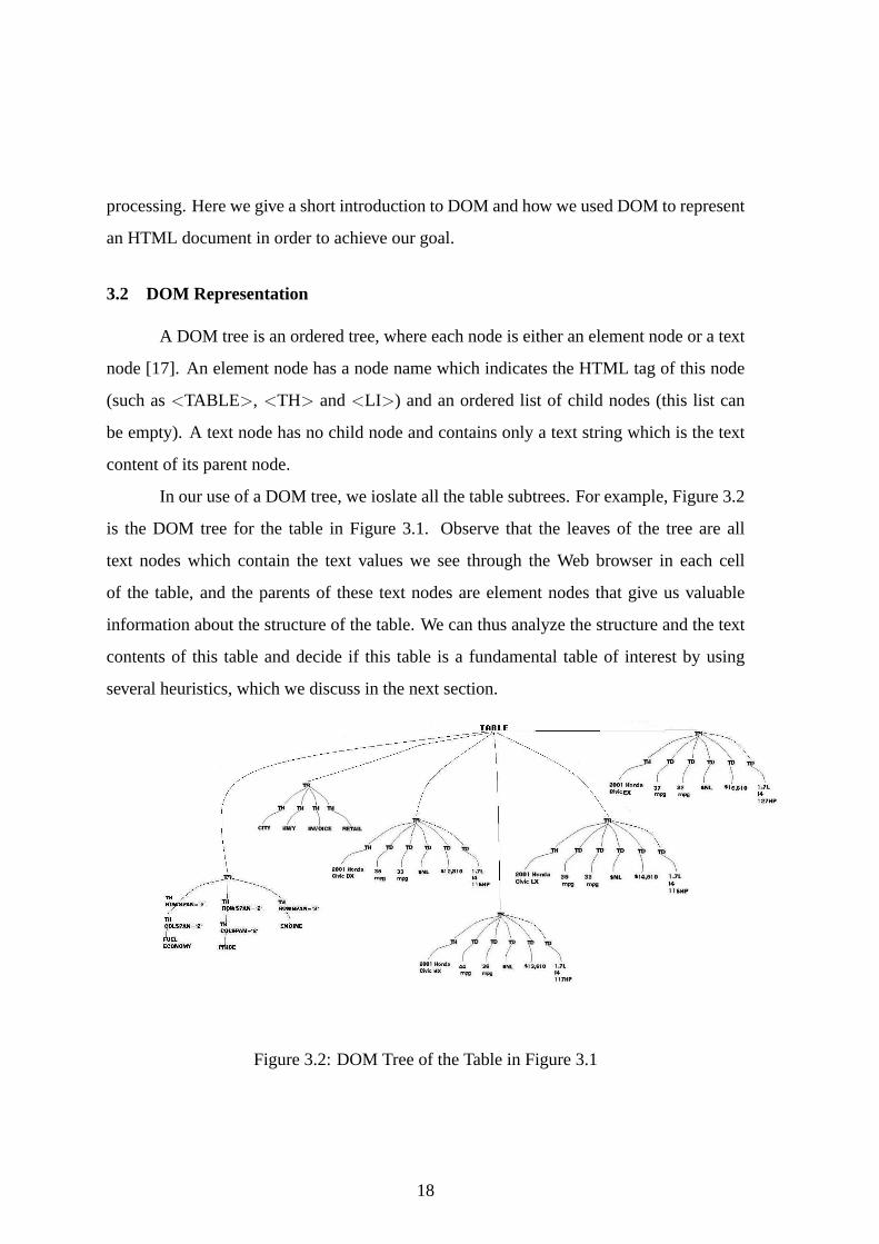
In our use of a DOM tree, we ioslate all the table subtrees. For example, Figure 3.2
is the DOM tree for the table in Figure 3.1. Observe that the leaves of the tree are all
text nodes which contain the text values we see through the Web browser in each cell
of the table, and the parents of these text nodes are element nodes that give us valuable
information about the structure of the table. We can thus analyze the structure and the text
contents of this table and decide if this table is a fundamental table of interest by using
several heuristics, which we discuss in the next section.
Figure 3.2: DOM Tree of the Table in Figure 3.1
18
3.3 Table Location Heuristics
Our table-location task is to find both the fundamental table of interest in the top-
level page (top-level Table) and the table(s) of interest in the linked pages. Since tables
of interest that appear in these two kinds of sources usually have different structures and
features (although they do, of course, share some common features), we treated them dif-
ferently by using two sets of heuristics.
3.3.1 Location – Top-Level Tables
In order to create a set of proper heuristics that covers as many cases as possible and
maintain high accuracy, we first gathered information about top-level tables by considering
several Web pages, which we call a “training set”2. Based on the training pages, we found
the following features of interest about top-level tables:
1. A table of interest must look like a table to a human observer.
2. A table of interest must have a schema-like3 row (or column) within the first few
rows (or columns).
3. A table of interest must contain enough information of interest (i.e. information that
our ontology recognizes).
Based on these features, we developed a set of heuristics for the main table-location
task. Our system resolves the problems of finding the main table of interest as follows.
• Table Size. The main table must have at least three rows and at least three columns.
As an example, by this heuristic, the system successfully discarded the table about
contact information and address in Figure 1.2.
• Grid Layout. We can count the number of data cells in each row in a table. Letting
N be the number of rows in the table that has the most common number of data cells2We used this set of pages to help us identify needed heuristics. (This is not a training set in the machine-
learning sense.)3Here, “schema-like” means a set of descriptive names that are like attributes in a relational table.
19
andM be the number of rows in the table, the ratioN/M must exceed2/3. This
ensures that the vast majority of the rows extend across the width of the table and
thus that the table, at least roughly, has the expected geometry of a table.
For example, suppose the table of interest in Figure 1.2 (the one in the middle with
attribute namesYear, Make and Model, Price, etc.) only has 9 columns. For the large
table which starts withPre-Owned Inventoryand ends with the email addressE-
mail:[email protected], there are 9 rows that contain 1 value,
9 rows that contain 6 values and 4 rows that contain 4 values. Therefore, the Grid
Layout Measure is 9/(9+9+4) = 0.41< 2/3. Thus, the system discards this large
table.
• Attributes. Based on the keywords and the object-set names for the various object
sets in our extraction ontology, we have a reasonable idea about what some of the
attribute names for a table should be. For example, we include possible synonyms
for each attribute such asMiles, Mi, andOdometerfor Mileage, andManufacture
andBrand for Make. We also include some popular attributes that commonly appear
in source tables but are not an attribute in our target schema because of a different
granularity. For example, we includeVehiclewhich could possibly represents several
target attributes such asMake, Model, andFeature; Trim which could be part of the
target attributeModel; andColor which could be one of the subsets for target attribute
Feature. We look for a row near the top which contains the most common number
of data cells and from which we have been able to extract 60% of the data entries as
attributes—these attributes, of course, must be distinct. (Note that we do not depend
on the table creator to mark the attributes with a<TH> tag.) If we cannot find an
attribute row in the table, we try columns, preferably leftmost columns. If we find
an attribute column, we can transpose the table so that the attributes are in rows.
By using this heuristic, the system can also discard the large table which starts with
Pre-Owned Inventoryand ends withE-mail:[email protected]
in Figure 1.2 (no matter how many columns the middle table contains) because it
cannot find an attribute row within the top few rows or columns.
20

• Value Density. Based on the values expected for the various lexical object sets, we
find all ontology-recognized strings. If the ratio of the number of characters in rec-
ognized strings to the total number of characters in strings within the table exceeds
10%, we have some reasonable evidence that the table is of interest for the applica-
tion. (Although 10% may seem low, previous experiments with density [25] show
that the density test should fail only for extremely low percentages, usually below
1%.) By using this heuristic, we ensure that the table contains some information of
interest.
3.3.2 Location – Linked-Page Tables
For tables in linked pages, table detection is different. Tables that appear in a linked
page usually are either anattribute-value-pair Tablesuch as the table under the car picture
starting withPrice$21,988in Figure 1.3, or asingle-attribute Tablestarting withFeatures
and on the left side of the car picture in Figure 1.3. We use the following heuristics for
these tables.
Attribute-Value-Pair Table
• Table Size. We do not expect sub-tables to be as large as top-level tables. Thus we
only require at least two rows or two columns.
• Attributes. This is the same as for top-level tables.
• Attribute-Value-PairTo locate table components that contain attribute-value pairs, we
look for a pair of columns where the strings in the first column have been extracted
mostly as attributes and the strings in the second column have been extracted mostly
as values. The table component in Figure 1.3 is an example—the left column starting
with Pricecontains many strings our extraction ontology recognizes as attributes, and
the right column starting with$21,988contains many strings our extraction ontology
recognizes as values. Sometimes these types of tables are folded, so we must consider
several pairs of columns side by side. As for other attribute tests, we use 60% as our
21

threshold. We also check for row pairs in the same way to locate table components
formatted with the attributes above the values, rather than to the left.
• Page-Spanning Tables. We follow a selected number of links from the top-level table
to obtain several linked table rows. We then check the variability—attributes tend
to remain the same from page to page (although sometimes table rows have more
or fewer attributes), while values tend to vary (although some, such as colors, body
styles, and transmission types are often identical).
Single-Attribute Table
To find lists like theFeatureslist in Figure 1.3, we look for a<UL> or an<OL>
tag or for a<TABLE> tag followed by a single-column table structure. We confirm that
the single-attribute table is of interest by checking whether the ontology recognizes at least
60% of the strings as values of interest.
3.4 Table Preprocessing and Understanding
After detecting tables of interest (both on the top page and on linked pages, if appli-
cable), the next step is to analyze the structure of these tables in order to fully “understand”
them (by “understanding”, we mean to associate values with their corresponding attributes
in the tables).
A top-level table sometimes contains multiple rows (or columns) of attributes, table
headers, table factors, or irrelevant information that needs to be ignored during extraction.
In order to extract this kind of information correctly, the system must understand the given
table properly and preprocess the table according the table structure. In this research, we
first try to find the attribute row(s) (or column(s)). According to the attribute position and
some other structural information, we can then locate table headers and factors and finally
associate attributes and values.
As discussed in the previous section, the system has already detected all the attribute
row(s) or column(s) for a table. We can make use of linked components of the top-level
table to help determine with certainty which strings are attributes and which are values by
22
observing that the attributes remain the same across pages while the values change. For
the page in Figure 1.2, for example, all subsequent pages linked byShow 25 morehave
identical attributes on the top row of the table, namelyYear, Make and Model, Price, Miles,
Exterior, Photo. Indeed, in this way, we are likely to be able to identify attributes, such as
Photo, even when they are not in our application ontology.
After determining the position of attributes, the system then determines the structure
of the table. In this research we only consider tables with attributes on the top or attributes
on the left. Since we can always convert an attributes-on-the-left table to an attributes-
on-the-top table or vice versa, in this section we just discuss tables with attributes on the
top.
We first list several pre-processing issues the system resolves.
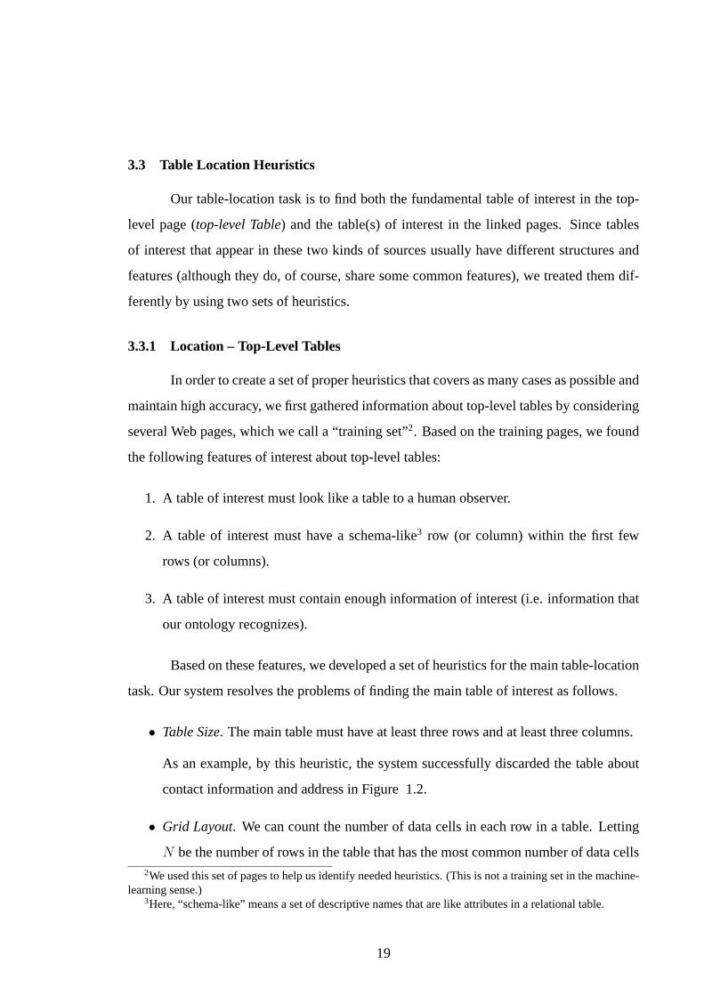
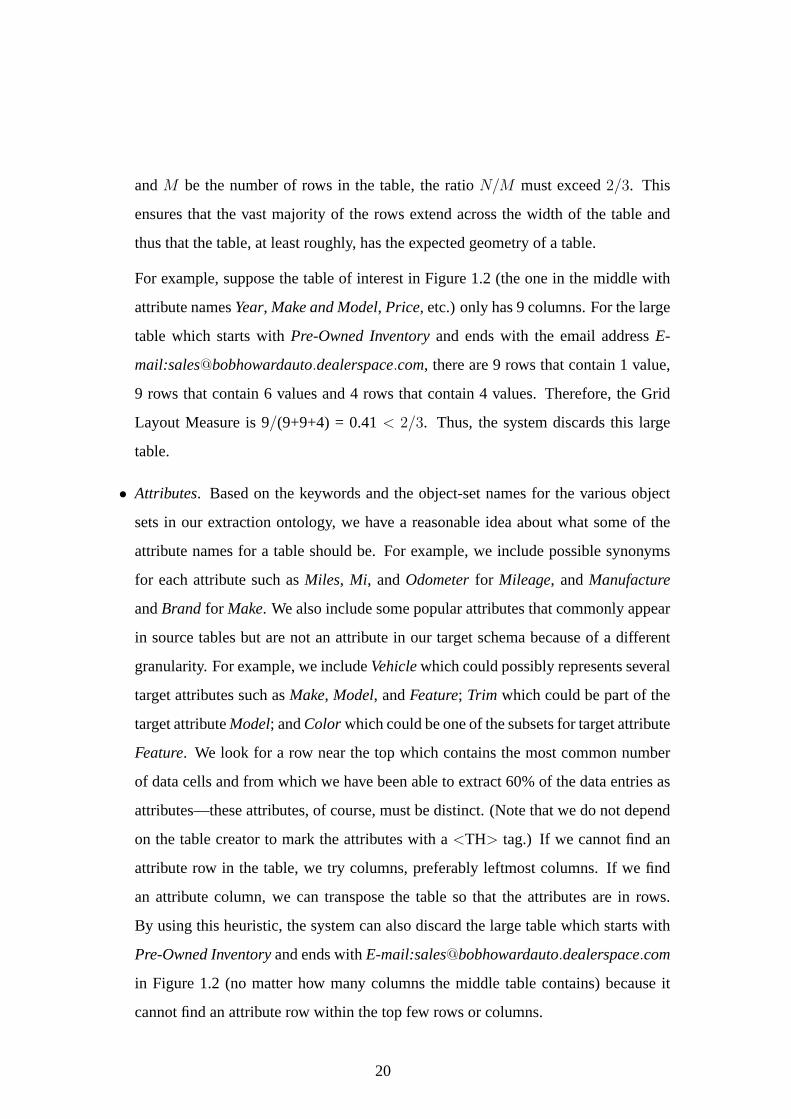
• Folded Tables. Figure 3.3 shows an example of a folded table in a linked page (folded
tables usually appear more frequently in linked pages than in top-level pages). Some-
times for layout reason or sometimes because a table has so many columns, table
designers fold them for viewing on a single page or in a single window either by
placing the second half of the columns below the first half of the columns or by mak-
ing two (or more) rows of attributes at the top that associate with pairs (triples, ...)
of values in the columns below. If more than one attribute row appears, we compare
the attribute rows. If they are not the same, we treat the table as a folded table; other-
wise we remove the duplicate attribute rows. For a folded table, we unfolded it and
appended the the second (and third, ...) folded part(s) to the first one. Thus, after
unfolding, the table in Figure 3.3 becomes the table in Figure 3.4.
• Factored Value Rows. We consider as possible factored values those values in each
table row where the row has less than half the cells filled and the cells that are filled
are adjacent left-most fields. Figure 3.5 shows an example of a table that has factors.
We add factored values that are below the attribute row to all subsequent rows until
the next row of factored values. For values that are above the attribute row, we check
if the row right below the attribute row is a factor row. If it is, then we consider all
the values above the attribute row as table headers, which we will discuss in the next
23

Figure 3.3: An Example of Folded Table in a Linked Page (www.jscars.com [35])
Figure 3.4: The Unfolded Table for the Table in Figure 3.3
24

paragraph. If it is not, then the row right above the attribute row is considered as a
factored value. Thus we also add these factored values to the all subsequent rows
(except the attribute row) until the next row of factored values. Figure 3.6 shows the
altered table for the table in Figure 3.5. We eliminate rows that do not satisfy these
factoring criteria—presumable these are not value table rows—for example, the row
of buttons at the bottom of the table in Figure 1.2.
Figure 3.5: An Example of an Internal Factor
• Table Header. A table header usually appears in a row above the attribute row. It
only appears once and is normally short. For example,Honda Civicis a table header
that factors all the cars in the table in Figure 3.7. Our system considers as table
headers those rows that are above the attribute row, marked by only one<TD> or
<TH>, and have not already been recognized as table factors. After detecting a table
header, the system adds a new column with an empty attribute and places the header
25
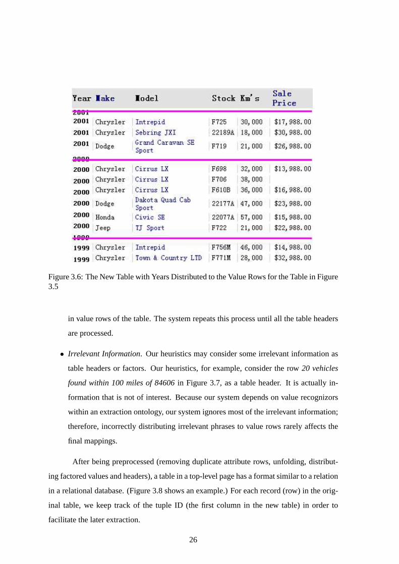
Figure 3.6: The New Table with Years Distributed to the Value Rows for the Table in Figure3.5
in value rows of the table. The system repeats this process until all the table headers
are processed.
• Irrelevant Information. Our heuristics may consider some irrelevant information as
table headers or factors. Our heuristics, for example, consider the row20 vehicles
found within 100 miles of 84606in Figure 3.7, as a table header. It is actually in-
formation that is not of interest. Because our system depends on value recognizors
within an extraction ontology, our system ignores most of the irrelevant information;
therefore, incorrectly distributing irrelevant phrases to value rows rarely affects the
final mappings.
After being preprocessed (removing duplicate attribute rows, unfolding, distribut-
ing factored values and headers), a table in a top-level page has a format similar to a relation
in a relational database. (Figure 3.8 shows an example.) For each record (row) in the orig-
inal table, we keep track of the tuple ID (the first column in the new table) in order to
facilitate the later extraction.
26
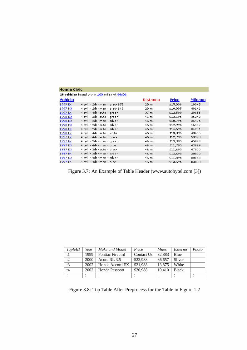
Figure 3.7: An Example of Table Header (www.autobytel.com [3])
TupleID Year Make and Model Price Miles Exterior Photot1 1999 Pontiac Firebird Contact Us 32,883 Bluet2 2000 Acura RL 3.5 $23,988 36,657 Silvert3 2002 Honda Accord EX $21,988 13,875 Whitet4 2002 Honda Passport $20,988 10,410 Black: : : : : : :
Figure 3.8: Top Table After Preprocess for the Table in Figure 1.2
27

TupleID Body Type Body Style Transmission Engine Fuel Type Stock Number VINt1t2t3 Car Coupe Automatic 3.0L 6 cyl Fuel Injection Gas 350291A 1H...644t4: : : : : : : :
Figure 3.9: Extended Table of the Information in Figure 1.3
Sometimes, each record (row) in the top-level table may have one or more links
that link to other pages. If tables have linked pages, they usually describe detailed infor-
mation for the corresponding top-level records, and each table describes information for
one record, as in Figure 1.3. As described in Section 3.3.2, tables that appear in a linked
page usually are either an attribute-value-pair table or a single-attribute table. We consider
these two kinds of tables as tables extending over several linked pages. Each table con-
tains values for one record over a set of attributes. Therefore we can collect values for the
“extended” table crossing linked pages.
For attribute-value-pair tables, consider the table under the car picture that starts
with Price $21,988in Figure 1.3 as an example. Figure 3.9 shows the extended table for
this example. The information in Figure 1.3 is for the third car in the table in Figure 1.2.
Observe that in Figure 3.9, we do not include all the attribute-value pairs that appear in the
attribute-value-pair table in Figure 1.3. AttributesPrice, MileageandExterior are already
in the top-level table, therefore the system does not duplicate them in the extended table.
Although attributeMile in the top-level table and attributeMileage in the linked-page are
not exactly the same, the system can detect these as synonyms with the help of keywords in
the ontology. In addition, at the value level, our ontology recognized the same value13,875
under these two attributes. Therefore, we know that these two attributes describe the same
information.
When we encounter an attribute-value-pair table in another linked page, we can
add values under their corresponding attribute in the specific position (according to their
tupleID). For example, if theBody Typefor the first car isSedan, we addSedanin the
second row (TupleID t1) under attributeBody Type. It is possible that the attribute-value
28
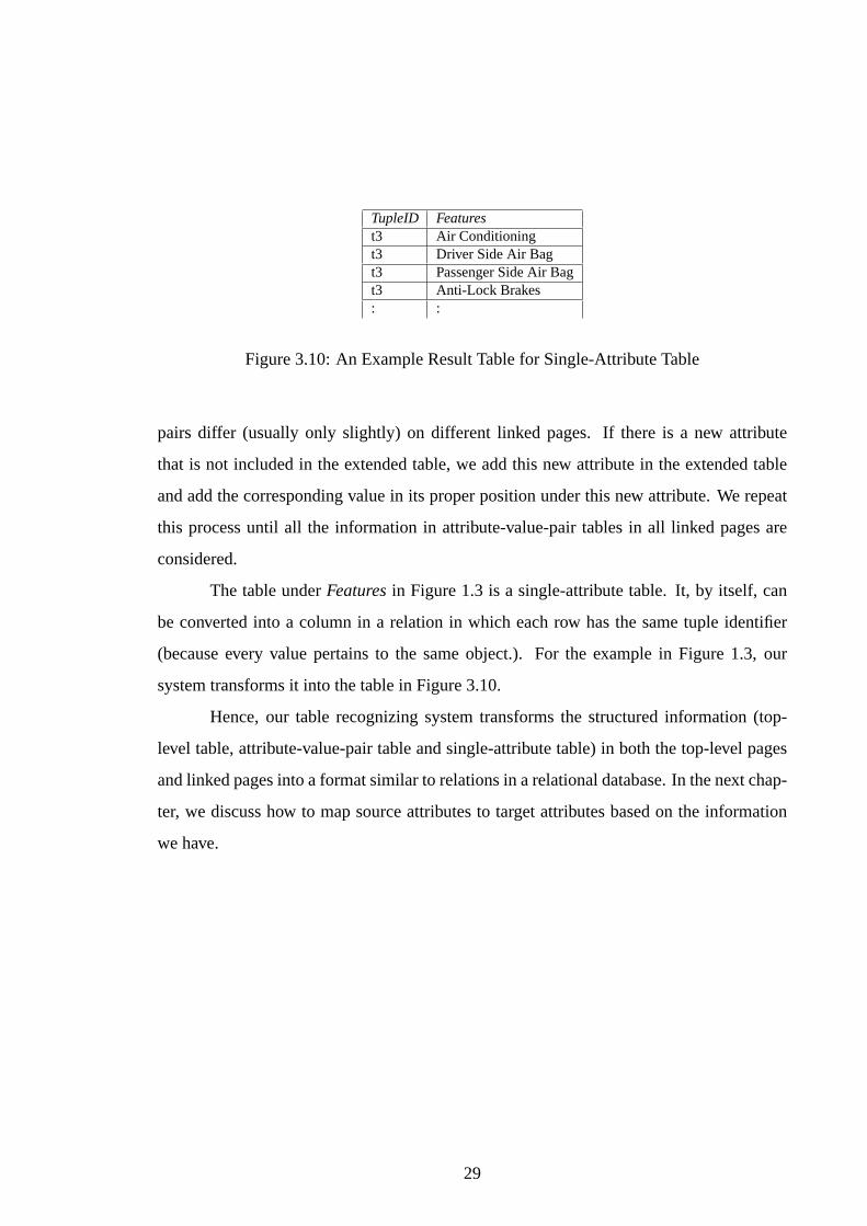
TupleID Featurest3 Air Conditioningt3 Driver Side Air Bagt3 Passenger Side Air Bagt3 Anti-Lock Brakes: :
Figure 3.10: An Example Result Table for Single-Attribute Table
pairs differ (usually only slightly) on different linked pages. If there is a new attribute
that is not included in the extended table, we add this new attribute in the extended table
and add the corresponding value in its proper position under this new attribute. We repeat
this process until all the information in attribute-value-pair tables in all linked pages are
considered.
The table underFeaturesin Figure 1.3 is a single-attribute table. It, by itself, can
be converted into a column in a relation in which each row has the same tuple identifier
(because every value pertains to the same object.). For the example in Figure 1.3, our
system transforms it into the table in Figure 3.10.
Hence, our table recognizing system transforms the structured information (top-
level table, attribute-value-pair table and single-attribute table) in both the top-level pages
and linked pages into a format similar to relations in a relational database. In the next chap-
ter, we discuss how to map source attributes to target attributes based on the information
we have.
29

30

Chapter 4
MAPPING INFERENCE
After preprocessing and understanding the table, the system has converted the struc-
tured information into one or more table structures that are similar to relations in a relational
database. We then can infer mappings from these source “relations” to the target object sets
in our extraction ontology (i.e. infer a mapping from source attributes to target attributes).
We infer mappings in two steps: (1) generate and adjust attribute-value pairs in preparation
for mapping recognition and (2) use patterns of recognized attributes and values to infer
mappings.
4.1 Generate and Adjust Attribute-Value Pairs
In one column in a source table, the attribute names the type of values under it.
Although we can sometimes determine the type of a value without an attribute, the attribute
often provides valuable context information for ontology extraction. Therefore, pairing a
value with its corresponding attribute may help our ontology recognize more information
from the table. For example, the attribute-value pairs we form for the attribute-value-pair
table in Figure 3.4 is:
{Year: 2002, Body: 4DR, A/C: Yes, Make: ISUZU, Motor: 6; Model: AXIOM 4WD,
Transmission: A, Miles: 26245}.
Observe that in this example, we may not be able to determine the type of some
values without their attributes such as values inMotor: 6 andTransmission: A. The digit6
and letterAmay not provide enough information by themselves without their corresponding
31
attributes. With the help of attributes, however, we can determine the type and meaning of
those values.
Another interesting issue our example shows isA/C: Yes— an attribute with a
Boolean value. We process Boolean values by replacing them with attribute-name val-
ues. For our running example, the adjusted attribute-value pairs become{Year: 2002,
Body: 4DR, A/C, Make: ISUZU, Motor: 6; Model: AXIOM 4WD, Transmission: A, Miles:
26245}. Here, the Boolean-valued attribute-value pair〈A/C: Yes〉 has becomeA/C, mean-
ing the car has A/C (air conditioning). If there is an attribute-value pair with valueno, we
simply replace it with an empty string, meaning the car does not have the feature indicated
by the attribute. For example, the first value row of the table in Figure 4.1a would be trans-
formed to{Make: ACURA, Model: legend, Yr: 1992, Colour: Grey, Price:$9500, Auto,
AM/FM }. Note that the attributesAir Cond.andCD disappeared because this car does not
have these features.
When attribute names are the values and the values are Boolean indicators (e.g.
Yes/No, True/False, 1/0, cell checked or empty,√
or x), we need to decide what the
Boolean indicators mean. We have a dictionary of Boolean indicators that defines po-
tential meanings for each indicator. For an indicator likeYesor No, we can know for sure
what they mean. Some other indicators, however, could have different meanings in differ-
ent situations. For example, anx could meanyeswhen an empty cell meansno; it also
could mean “no” when a√
meansyes. If a Boolean value is in the dictionary, we check
the potential meaning of the indicator. If the indicator has only one meaning, we assign the
opposite meaning to the other Boolean value (if any) in the same column. If it has more
than one meaning, we then need to check the other Boolean value that appears in the same
column. For example, if we encounter anx, and it has two meanings:yesandno, in the
dictionary, we then check other operators in the same column. For example, we found a√
,
which has only one meaning,yes, in the dictionary. We then can decide thex here does not
meanyes, but meansno. Based on this heuristic, we can understand what a pair of Boolean
indicators mean as long as we can find them in our dictionary.
32
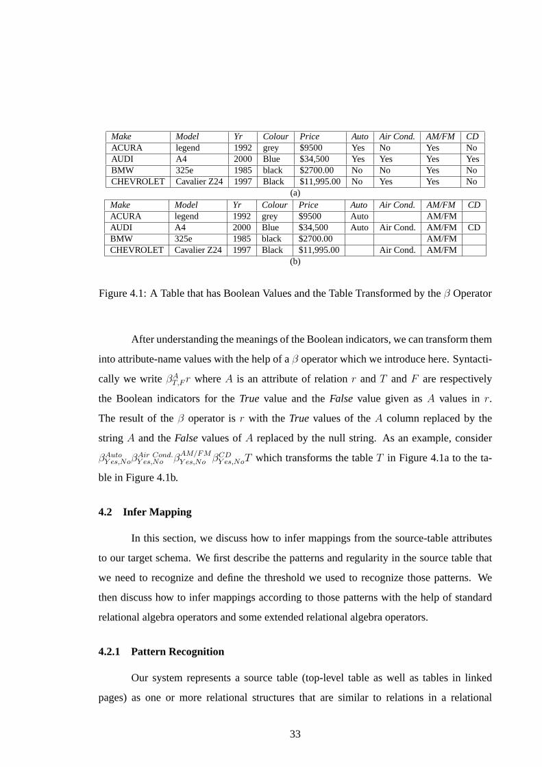
Make Model Yr Colour Price Auto Air Cond. AM/FM CDACURA legend 1992 grey $9500 Yes No Yes NoAUDI A4 2000 Blue $34,500 Yes Yes Yes YesBMW 325e 1985 black $2700.00 No No Yes NoCHEVROLET Cavalier Z24 1997 Black $11,995.00 No Yes Yes No
(a)Make Model Yr Colour Price Auto Air Cond. AM/FM CDACURA legend 1992 grey $9500 Auto AM/FMAUDI A4 2000 Blue $34,500 Auto Air Cond. AM/FM CDBMW 325e 1985 black $2700.00 AM/FMCHEVROLET Cavalier Z24 1997 Black $11,995.00 Air Cond. AM/FM
(b)
Figure 4.1: A Table that has Boolean Values and the Table Transformed by theβ Operator
After understanding the meanings of the Boolean indicators, we can transform them
into attribute-name values with the help of aβ operator which we introduce here. Syntacti-
cally we writeβAT,F r whereA is an attribute of relationr andT andF are respectively
the Boolean indicators for theTrue value and theFalse value given asA values inr.
The result of theβ operator isr with the True values of theA column replaced by the
string A and theFalsevalues ofA replaced by the null string. As an example, consider
βAutoY es,Noβ
Air Cond.Y es,No β
AM/FMY es,No βCD
Y es,NoT which transforms the tableT in Figure 4.1a to the ta-
ble in Figure 4.1b.
4.2 Infer Mapping
In this section, we discuss how to infer mappings from the source-table attributes
to our target schema. We first describe the patterns and regularity in the source table that
we need to recognize and define the threshold we used to recognize those patterns. We
then discuss how to infer mappings according to those patterns with the help of standard
relational algebra operators and some extended relational algebra operators.
4.2.1 Pattern Recognition
Our system represents a source table (top-level table as well as tables in linked
pages) as one or more relational structures that are similar to relations in a relational
33
database. The values in each relational structure are formatted as attribute-value pairs and
each Boolean value is transformed into a proper value. Based on this source representa-
tion, we infer mappings by using our ontology-extraction technology. As we mentioned in
Chapter 2, our extraction ontology is source independent, which means we do not have to
generate a new ontology when a new source document is encountered. It is hard, however,
to guarantee that our ontology covers everything. We do not expect our system to recog-
nize all the source values. Instead, our purpose is to find data regularity and infer mappings
depending on the recognized results.
Because of the special layout structured tables have, we know all the values un-
der a single attribute in a source table should be extracted to a same attribute or set of
attributes in the target schema. Given the recognized extraction and its regularity in the
source document, our system can measure how many values under a source attribute are
actually extracted to a particular set of target attributes. If the number is greater than a
threshold, the system can infer mappings between source and target attributes according to
the regularity observed. Given a set of mappings, the system can then extract data into the
target database, including not only the recognized values, but also all other values that fit
the pattern. By doing so, we are likely to be able to increase both the precision and recall
of the extraction. We talk about the experimental results in detail in Chapter 5.
In order to infer as many correct mappings as possible and, at the same time, avoid
unnecessary incorrect mappings, an appropriate threshold is important. A high threshold
would result in the low mapping rates (low recall) while a low threshold would result in
many error mappings (low precision). In this thesis, we define the threshold to be the
Golden Mean, also called the “divine proportion”[2]. This constant can be calculated by
(√
5 -1)/2 ≈ 0.618. The term ”Golden Mean” is derived from Horace’s Latin transla-
tion of “aurea mediocratas,” which means a sensible way of doing things or the avoidance
of extremes. In mathematics and real life, the Golden Mean often represents a balanced
threshold [2]. Therefore, in our research, we also use this ratio as our threshold.
34
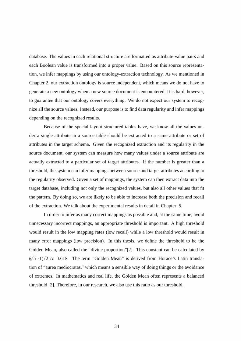
1. Make matches [10]2. constant3. { extract " \bacura \b"; },4. { extract " \balfa(( \s*|-)romeo)? \b"; },5. { extract " \bamc\b"; },6. { extract " \bam(\s*|-)general \b"; },7. { extract " \baudi \b"; },8. { extract " \bbentley \b"; },9. { extract " \bbertone \b"; },10. { extract " \bbmw\b"; },11. { extract " \bbuick \b"; },12. { extract " \bcad(illac)? \b"; },13. { extract " \bchev(y|rolet)? \b"; },14. { extract " \bchrysler \b"; },15. ...
Figure 4.2: Data Frame for the Make Object Set in Car-Ads Extraction Ontology (Partial)
4.2.2 Mapping Inference
Our purpose is to match source table attributes with target attributes (object sets
in the ontology). As discussed in Chapter 2, an extraction ontology contains information
about object sets, relationships, and data frames. Each object set has a data frame that
defines the potential contents of the object set. A data frame for an object set defines the
lexical appearance of constant objects for the object set and establishes appropriate key-
words that are likely to appear in a document when objects in the object set are mentioned.
In order to find mappings from source attributes to the object sets, we apply each data
frame to each column in the source table to see if we recognize enough values, so that the
percentage of recognized values is greater than the threshold.
Figure 4.2 shows a partial data frame for object setMakein our car ontology. Now
let us see if there is any attribute in Figure 4.1 from which we can map this object set. We
attempt to recognize values in each column in Figure 4.1 with regular expressions in the
Makedata frame, and we keep track of the number recognized. In our example, for the
first column we recognized 100% (e.g.ACURAmatches using Line 3 in Figure 4.1,AUDI
matches using Line 7,BMW matches using Line 10 andCHEVROLETmatches using Line
13). For the rest of columns, however, we recognized nothing. Therefore, we can infer
35
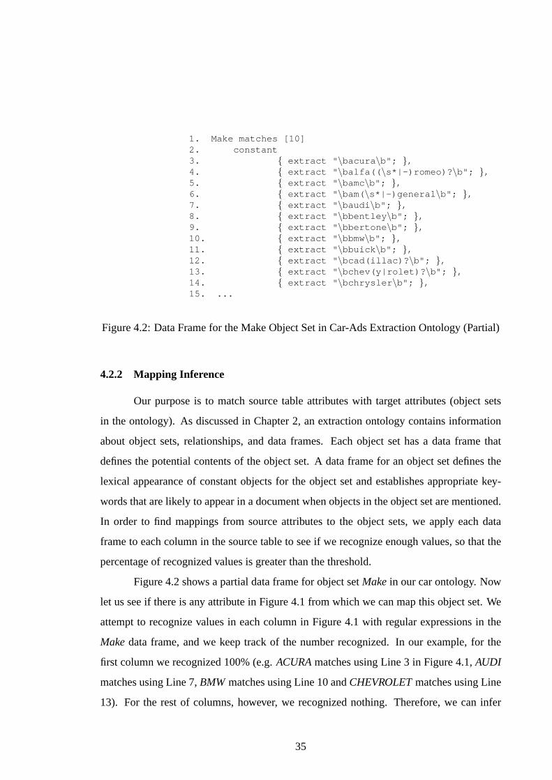
Make ModelHonda CivicNissan Sentra
Figure 4.3: Columns Added to the Table in Figure 4.4 by theδ Operator
a mapping fromMake in the source table toMake in the target ontology. This is a direct
mapping. Similarly, we can obtain mappings fromModel to Model, Yr to Year, andPrice
to Price. The mapping fromYr to Year, however, is not a direct mapping, because we need
a renaming operatorρ.
Except for simple renaming, indirect mappings are more complicated, and the sys-
tem needs the help of more operators. As we can see, values in the 6th-9th columns in
Figure 4.1 should all go under a single target attributeFeature. In this case, the system
needs to gather them together and consider each of them as a separate value under one
target attribute. We gather values together with the union operator∪.
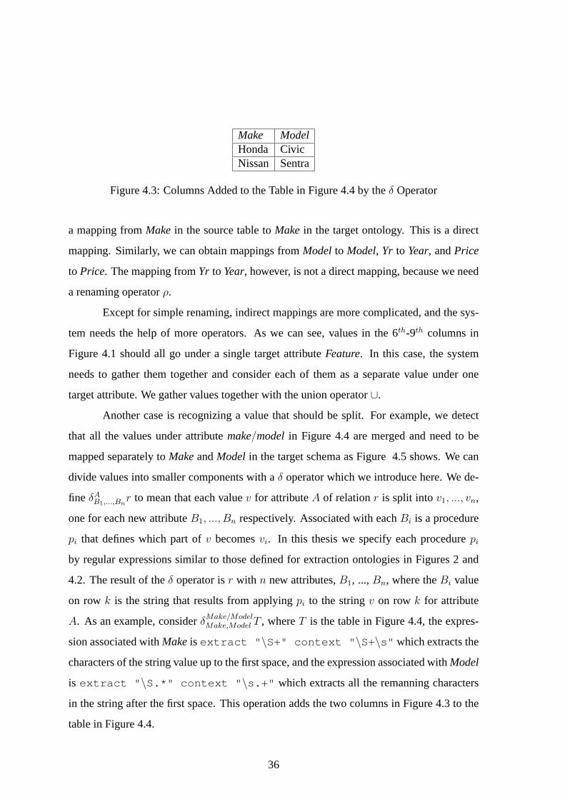
Another case is recognizing a value that should be split. For example, we detect
that all the values under attributemake/model in Figure 4.4 are merged and need to be
mapped separately toMakeandModel in the target schema as Figure 4.5 shows. We can
divide values into smaller components with aδ operator which we introduce here. We de-
fine δAB1,...,Bn
r to mean that each valuev for attributeA of relationr is split intov1, ..., vn,
one for each new attributeB1, ..., Bn respectively. Associated with eachBi is a procedure
pi that defines which part ofv becomesvi. In this thesis we specify each procedurepi
by regular expressions similar to those defined for extraction ontologies in Figures 2 and
4.2. The result of theδ operator isr with n new attributes,B1, ...,Bn, where theBi value
on row k is the string that results from applyingpi to the stringv on row k for attribute
A. As an example, considerδMake/ModelMake,Model T , whereT is the table in Figure 4.4, the expres-
sion associated withMakeis extract " \S+" context " \S+\s" which extracts the
characters of the string value up to the first space, and the expression associated withModel
is extract " \S.*" context " \s.+" which extracts all the remanning characters
in the string after the first space. This operation adds the two columns in Figure 4.3 to the
table in Figure 4.4.
36

year make/model color bodytype1999 Honda Civic Green 4 dr sedan1998 Nissan Sentra grey 2 door coupe
Figure 4.4: An Sample Source Table
Car Year Make Model Mileage Price PhoneNr0001 1999 Honda Civic0002 1998 Nissan Sentra
Car Feature0001 Green0001 4 dr0001 sedan0001 grey0002 2 door0002 coupe
Figure 4.5: Extracted Result from the Table in Figure 4.4
If we consider the right-most table in Figure 4.5 as the source table and the schema
in table in Figure 4.4 as the target schema, we encounter another issue. Values under the a
same attribute need to be associated with different target attributes. In our example,Green
andgrey under the source attributeFeatureassociate with the target attributecolor, and
other values underFeatureassociate withfeaturesin target. In this case, we need to apply
a selection operatorσ. Here theσ operator is not standard because it may have a regular
expression as an argument. The selection operatorσA∼er selects those rows in a relation r
whose values under attribute A contain a string recognized by regular expression e.
Sometimes, the values of interest are scattered in unstructured or semistructured
documents. For this kind of direct extraction we introduce theε operator, which is based
on a given extraction ontology. We defineεSt as an operator that extracts a value, or values,
from unstructured or semistructured textt for object setS in the given extraction ontology
O according to the extraction expression forS in O. Theε operator extracts a single value
if S functionally depends on the object of interestx in O, and it extracts multiple values if
S does not functionally depend onx. As an example,εPhoneNrP extracts1-877-944-2842
from the unstructured text in pageP in Figure 1.3 and returns it as the single-attribute,
single-tuple, constant relation{PhoneNr: 1-877-944-2842}. We can use theε operator in
conjunction with a natural join to add a column of constant values to a table. For example,
37
T1 Make Model Trim T2 Make Model Trim Model with TrimFord Contour GL Ford Contour GL Contour GLFord Taurus LX Ford Taurus LX Taurus LXHonda Civic EX Honda Civic EX Civic EX
Figure 4.6: Application of theγ Operator to TableT1 Yielding TableT2
assuming the phone number1-877-944-2842appears in pageP with the table in Figure 1.2,
which indeed it does, we could applyεPhoneNrP 1 T to add a column forPhoneNrto
tableT in Figure 1.2.
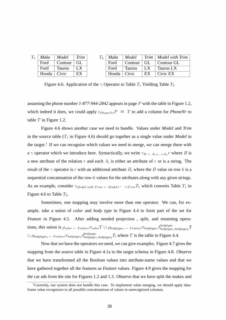
Figure 4.6 shows another case we need to handle. Values underModel andTrim
in the source table (T1 in Figure 4.6) should go together as a single value underModel in
the target.1 If we can recognize which values we need to merge, we can merge them with
a γ operator which we introduce here. Syntactically, we writeγB ← A1+...+Anr whereB is
a new attribute of the relationr and eachAi is either an attribute ofr or is a string. The
result of theγ operator isr with an additional attributeB, where theB value on rowk is a
sequential concatenation of the row-k values for the attributes along with any given strings.
As an example, considerγModel with Trim ← Model+" " +TrimT1 which converts TableT1 in
Figure 4.6 to TableT2.
Sometimes, one mapping may involve more than one operator. We can, for ex-
ample, take a union ofcolor and body typein Figure 4.4 to form part of the set for
Feature in Figure 4.5. After adding needed projection , split, and renaming opera-
tions, this union isρcolor ← FeatureπcolorT ∪ ρbodytype1 ← Featureπbodytype1δbodytypebodytype1,bodytype2
T
∪ ρbodytype2 ← Featureπbodytype2δbodytypebodytype1,bodytype2
T, whereT is the table in Figure 4.4.
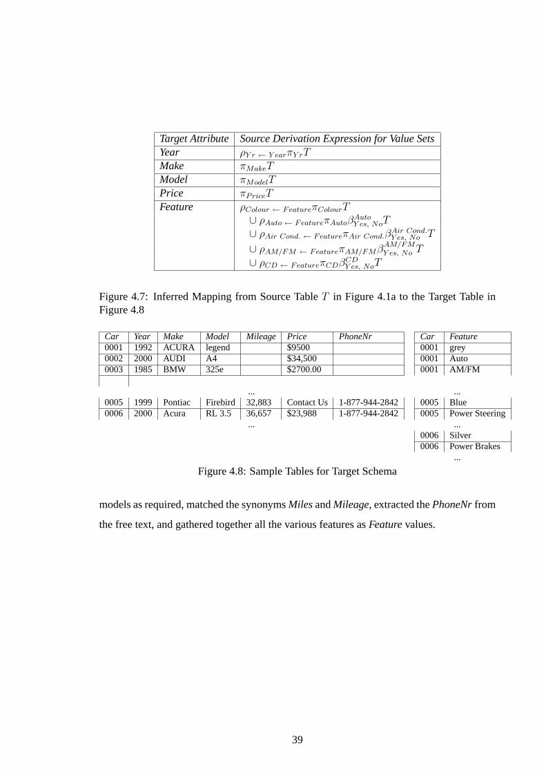
Now that we have the operators we need, we can give examples. Figure 4.7 gives the
mapping from the source table in Figure 4.1a to the target schema in Figure 4.8. Observe
that we have transformed all the Boolean values into attribute-name values and that we
have gathered together all the features asFeaturevalues. Figure 4.9 gives the mapping for
the car ads from the site for Figures 1.2 and 1.3. Observe that we have split the makes and
1Currently, our system does not handle this case. To implement value merging, we should apply data-frame value recognizers to all possible concatenations of values in unrecognized columns.
38
Target Attribute Source Derivation Expression for Value SetsYear ρY r ← Y earπY rTMake πMakeTModel πModelTPrice πPriceTFeature ρColour ← FeatureπColourT
∪ ρAuto ← FeatureπAutoβAutoY es, NoT
∪ ρAir Cond. ← FeatureπAir Cond.βAir Cond.Y es, No T
∪ ρAM/FM ← FeatureπAM/FMβAM/FMY es, No T
∪ ρCD ← FeatureπCDβCDY es, NoT
Figure 4.7: Inferred Mapping from Source TableT in Figure 4.1a to the Target Table inFigure 4.8
Car Year Make Model Mileage Price PhoneNr Car Feature0001 1992 ACURA legend $9500 0001 grey0002 2000 AUDI A4 $34,500 0001 Auto0003 1985 BMW 325e $2700.00 0001 AM/FM
... ...0005 1999 Pontiac Firebird 32,883 Contact Us 1-877-944-2842 0005 Blue0006 2000 Acura RL 3.5 36,657 $23,988 1-877-944-2842 0005 Power Steering
... ...0006 Silver0006 Power Brakes
...
Figure 4.8: Sample Tables for Target Schema
models as required, matched the synonymsMilesandMileage, extracted thePhoneNrfrom
the free text, and gathered together all the various features asFeaturevalues.
39

Target Attribute Source Derivation Expression for Value SetsYear πY earTMake πMakeδ
Make and ModelMake, Model T
Model πModelδMake and ModelMake, Model T
Mileage ρMiles ← MileageπModelTPrice πPriceTPhoneNr εPhoneNrP 1 TFeature ρExterior ← FeatureπExteriorT
∪ ρBody Type ← FeatureT’∪ ρBody Style ← FeatureT’∪ ρTransmission ← FeatureT’∪ ρEngine ← FeatureT’∪ ρFuel Type ← FeatureT’∪ ρFeatures ← FeatureT”
Figure 4.9: Inferred Mapping from the Source TablesT in Figure 1.2,T ′ in Figure 3.9, andT ′′ in Figure 3.10 and from P, the page in in Figure 1.2, to the Target Table in Figure 4.8
40

Chapter 5
EXPERIMENTAL ANALYSIS
We now present the results of two experiments in the domains of car advertisements
and cell phones.
5.1 Car Advertisements
We gathered tables of car advertisements from more than a hundred different English-
language Web sites. Because of human resource limitations, however, we analyzed only
60.
Of the 60 car-ads tables we analyzed, 28 included links to other pages containing
additional information about an advertised car (Figures 1.2 and 1.3 show a typical exam-
ple). For all 60 tables, we first applied our system to identify and list attribute-value pairs
for tuples of top-level tables, and then for the 28 tables with links, we appropriately asso-
ciated linked information with each tuple. We then applied our extraction step and looked
for mapping patterns.
Since our objective was to obtain mappings (rather than data), it was not necessary
for us to process every tuple in every table. Hence, from every table, we processed only the
first 10 car ads. As a threshold, we required six or more occurrences of a pattern to declare
a mapping. A human expert judged the correctness of each mapping.1 We considered a
mapping declaration for a target attribute to be completely correct if the pattern recognized
led to exactly the same mapping as the human expert declared, partially correct if the pattern
led to a unioned (or intersected) component of the mapping, and incorrect otherwise. For
1Although expert judgement for tables can sometimes be hard [31], establishing correctness results forcar-ads for our target table was not difficult.
41

data outside of tables, the system mapped an individual value to either the right place or
the wrong place or did not map a value it should have mapped.
5.1.1 Results—Car Advertisements
We divided the 60 car-ads tables into two groups: 7 “training” tables and 53 “test”
tables. We used the 7 “training” tables to generate the heuristics we used in table locating
and table understanding. For the 7 training tables, we were able to locate 100% of the top-
level tables as well as all the applicable tables in the linked pages. For the 53 test pages,
we were able to locate 46 top-level tables successfully (86.8%). Among these 46 tables,
28 had links to additional pages with more detail about each car ad. Of the 28 additional
pages, 13 had structured car-ad information, while 15 included unstructured information
(which is fine for data extraction, but does not apply for generating table mappings). The
system correctly analyzed 12 out of the 13 linked pages of structured information; it also
incorrectly declared that it found structured information in 2 linked pages.
We also analyzed our mapping approach for successfully located tables from the
test set. For the 46 recognized tables, there were 319 mappings, of which we correctly or
partially correctly discovered 296 (92.8%), missing 23 (7.2%); we (incorrectly) declared
13 false mappings (4.2% of 309 declared mappings). Of the correct mappings, 228 of
296 (77%) came from top-level tables, while 58 (19.6%) came from linked tables, and 10
(3.4%) came from both top-level and linked tables. Of the 296 mappings we correctly
discovered, 121 (40.9%) were direct matches, in the sense that the attributes in the source
and target schemas were identical, and 175 (59.1%) were indirect matches. Of the 175
indirect matches, 28 used synonyms and thus required only renaming with aρ operator,
1 had Boolean values and thus required aβ operator, 93 included features scattered un-
der various attributes and in raw text and thus required∪ andε operators, 2 provided only
factored telephone numbers and thus requiredε and1 operators, 53 needed to be split
and thus required aδ operator, and some required combinations of these operators (e.g.
synonyms and union). The values we needed to split came in a variety of different combi-
nations and under a variety of different names. We found, for example,Descriptionas an
42

attribute for the combinationYear+Make+Model+Feature, Model Coloras an attribute for
Make+Model+Color, andModelas an attribute forYear+Make+Model.
Discussion—Car Advertisements
Locating the correct table and understanding it properly is not a trivial problem. As
we discussed in Chapter 3, we consider attributes, values, and table layout when seeking
a table. Our system failed to locate 7 out of 53 test tables. All but one of the 7 missed
tables contained uncommon attributes in the source page. For example, some Web sites
use abbreviations likePW, PL, CC, andAC; others include attributes that are irrelevant to
the extraction ontology, such asImage, Click on Thumbnail, andLocation. This caused
our system to fail to detect an attribute row (or column) in a table, leading to a failure to
identify the correct table. The other table-location failure occurred because the top table
only had 2 columns, but we required a minimum size of 3 columns by 3 rows.
For linked pages, the system was not able to find the correct table (single attribute-
value pairs) for one site (out of 13). This is because all cars shared a single linked page
containing information for all the cars (a case we had not considered). Our system in-
correctly identified two linked pages as containing tables of interest because it interpreted
some values as attributes or vice versa.
As mentioned in our earlier discussion, discovering correct mappings can lead to
an increase in values extracted compared to what would have been found by the extraction
ontology alone and can also therefore lead to the acquisition of additional knowledge for the
extraction ontology. In our experiments, we required 60% of the values to match to declare
a mapping. Overall, we actually achieved roughly 90–95%, a much higher percentage.
This, however, leaves about 5–10% of the approximately 3,000 values encountered in tables
as being unrecognized by the extraction ontology (and potentially many hundreds more
since we processed only 10 car ads per site). Examples include non-U.S. models such as the
Toyota Starletor Nissan Presea; elaborately described features such astelescoping steering
wheel; abbreviations not encountered previously such asleath int for leather interior; and
features simply not encountered before, such astrip computer.
43

We missed 23 mappings and only declared 13 false mappings. Our system missed
10 mappings of car model because the extraction ontology was targeted to U.S. car ads,
and so non-U.S. ads introduced car models that our system did not recognize. The sys-
tem missed 2 price mappings, 1 mileage mapping, and 2 feature mappings because the
extraction ontology was overly restrictive. All of these problems can be corrected by minor
adjustments to the extraction ontology. The system missed another 5 mappings because of
bugs in the original documents (ill-formed HTML) or due to the use of special codes to in-
dicate particular values like colors. Sometimes Web sites use generic “filler” values such as
contact us, please call, or unknowninstead of listing actual prices, mileages, and so on; we
missed 3 mappings for this reason. For the 13 incorrect mappings, 8 came from incorrectly
understood linked pages. One of these 8, for example, mapsLocationto Model, because
the location isAurora (a city in Colorado) which is also a model name for Oldsmobile. The
other primary confusion for our tool was distinguishing between numbers such as price and
mileage.
5.1.2 Cell-Phone Sales
The car-advertisements example uses our most mature extraction ontology, and so
we expected to achieve good results using it. To see how our table understanding ap-
proach works with less developed extraction ontologies, we tested our system in the U.S.
cell-phone sales domain. Figure 5.1 shows part of a top page of a typical cellular-phone ap-
plication, and Figure 5.2 shows part of a page obtained by clicking onMlife Local $29.99.
We used the following target schema:
{Plan, Carrier, MonthlyFee, AnyTimeMin, OffPeakMin, ContractLength,
ActivationFee CancellationFee}{Plan, Feature}.
Similar to our car-ads experiment, we started with a training set of 5 cell-phone
Web pages, and we tuned our extraction ontology to handle these 5 cases. We then gathered
pages from 12 cell-phone Web sites for our test set, and found that our tool correctly located
top-level tables in 11 of them (91.7%). The table that was missed was excluded because it
44
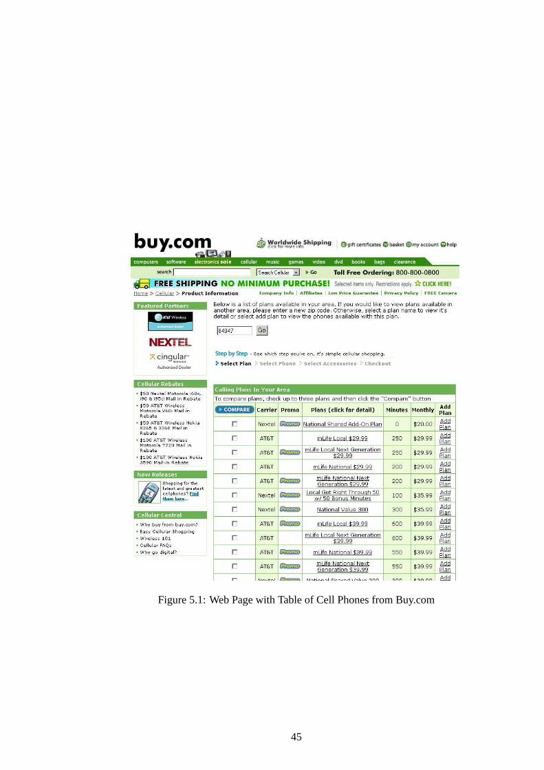
Figure 5.1: Web Page with Table of Cell Phones from Buy.com
45
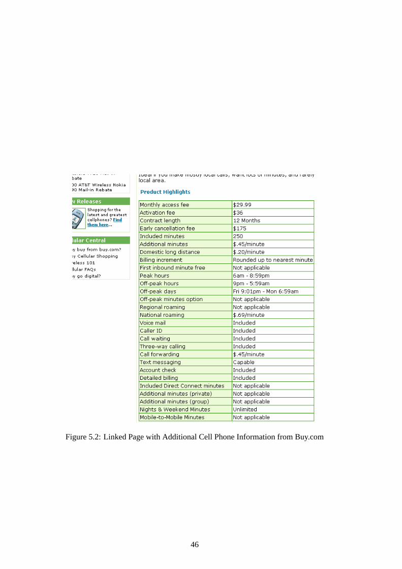
Figure 5.2: Linked Page with Additional Cell Phone Information from Buy.com
46

only had two columns, thus failing our minimum size threshold of 3 rows and 3 columns.
There were also 4 linked pages, all of which contained relevant tables that our tool properly
located. A human expert judged that there were 97 mappings relevant to our extraction
ontology in the 11 sites for which we correctly identified the top-level table. Our system
declared 103 mappings, of which 15 were false mappings (14.6%), and 88 were correct or
partially correct mappings (85.4%). In this experiment, 48 mappings came from top-level
tables (46.6%), while 52 came from linked pages (50.5%), and 3 came from both top-level
and linked pages. Our system missed 9 mappings (9.3% of 97).
Of the 15 false mappings, 6 came from linked tables, and in all cases these were for
the target attributeOffPeakMin. The other 9 false mappings came from top-level tables: 5
for AnyTimeMin, 2 for ActivationFee, and 1 each forCancellationFeeandOffPeakMin. In
all cases, the false mappings were related to numeric attributes. With more context infor-
mation in the extraction ontology, our tool could do a better job distinguishing the meaning
of different numbers. As expected, the false-positive rate for the cell-phone domain is sev-
eral times higher than for car ads (14.6% versus 4.2%), which can be attributed partially
to the relative amount of effort spent in developing the corresponding extraction ontolo-
gies, and partially to the high degree of similarity between the domains of attributes in the
cell-phone application.
An interesting aspect of the cell-phone domain is that of the 88 mappings we cor-
rectly discovered, none were direct (as compared to 40.9% for car ads). That is, we had
to apply some transformation operator to every mapping in the cell-phone application: 38
mappings used synonyms and thus required aρ operator for renaming; 34 mappings in-
cluded features scattered under various attributes, and thus required∪ operators; and 24
mappings needed to be split and thus required aδ operator. Some mappings required com-
binations of operators.
The overall performance of our tool in the cell-phone sales domain is reasonably
good and generally in line with our expectations. We could improve the outcome by tuning
the extraction ontology more carefully.
47

48

Chapter 6
CONCLUSIONS AND FUTURE WORK
6.1 Conclusions
In this thesis, we designed and implemented a system which can automatically
locate HTML tables for a specified application domain and then extract information of
interest from the located tables by inferring mappings from source tables to a target schema.
We suggested a different approach to the problem of schema matching, one which may
work better for the heterogeneous HTML tables encountered on the Web. In essence, we
transformed the table location problem and the schema matching problem into an extraction
problem that provides information to distinguish tables from surrounding text and layout,
and to infer the semantic correspondence between a source table and a target schema. We
gave experimental evidence to show that our approach can be successful. In particular,
we tested two applications: car advertisements and cell-phone sales. We correctly located
90% of the tables (top-level and linked) in pages for these two applications. Then, from
the located tables we inferred 93% of the appropriate mappings with a precision of 96%
for our car-ads application and inferred 91% of the appropriate mappings with a precision
of 85% for our cell-phone application.
6.2 Future Work and Interesting Unresolved Table Problems
As a next step of the table location and understanding problem, we would like to
improve our approach and make it handle more cases such as some of the problems listed in
Appendix A. We also do not want to just focus on HTML tables. To locate and understand
tables in other formats is also an interesting problem.
49
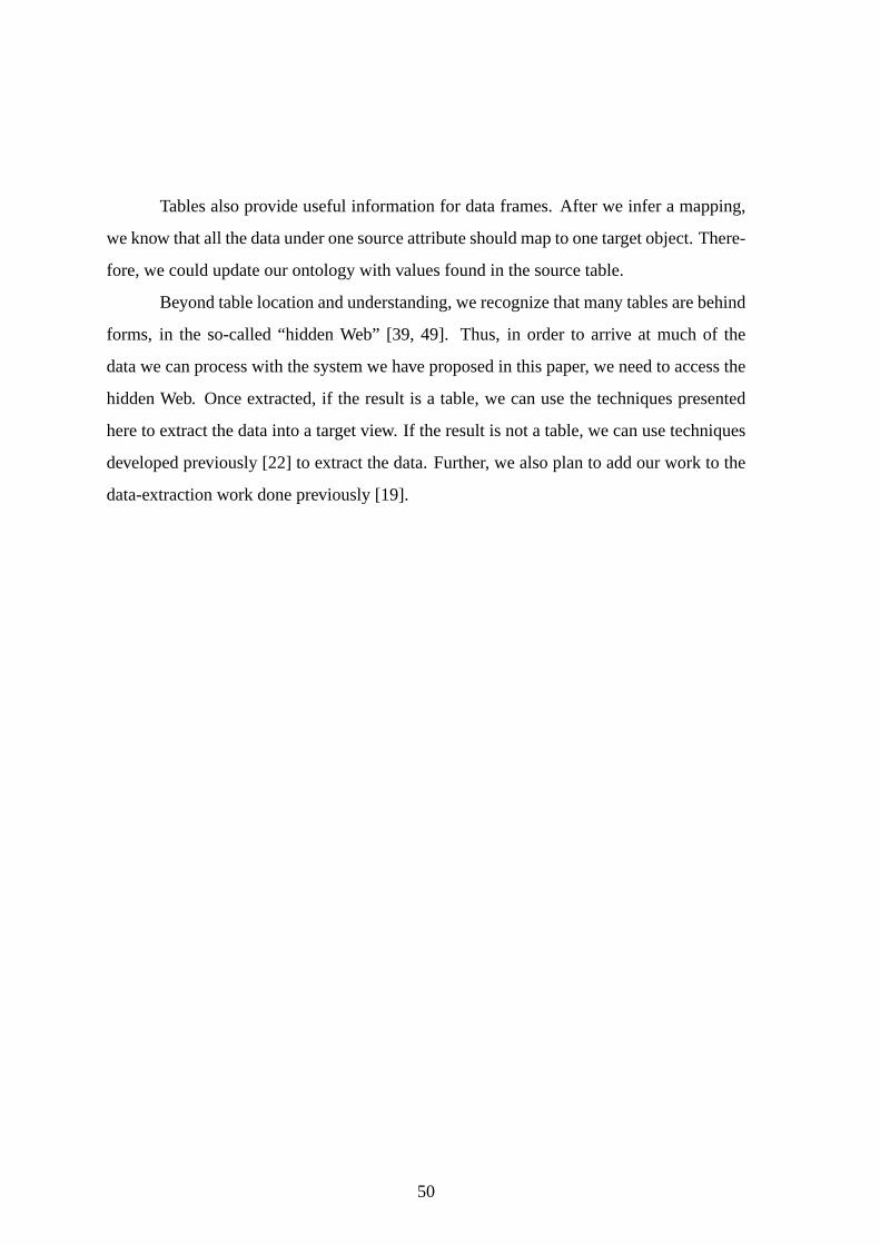
Tables also provide useful information for data frames. After we infer a mapping,
we know that all the data under one source attribute should map to one target object. There-
fore, we could update our ontology with values found in the source table.
Beyond table location and understanding, we recognize that many tables are behind
forms, in the so-called “hidden Web” [39, 49]. Thus, in order to arrive at much of the
data we can process with the system we have proposed in this paper, we need to access the
hidden Web. Once extracted, if the result is a table, we can use the techniques presented
here to extract the data into a target view. If the result is not a table, we can use techniques
developed previously [22] to extract the data. Further, we also plan to add our work to the
data-extraction work done previously [19].
50

Bibliography
[1] www.ads4autos.com, July 2003.
[2] P. G. Anderson. Multidimensional golden means. InApplications of Fibonacci num-
bers, Vol. 5 (St. Andrews, 1992), pages 1–9. Kluwer Academic Publishers Group,
Dordrecht, 1993.
[3] Autobytel.com, Spring 2001.
[4] www.autoexecutives.com, July 2003.
[5] autoscanada.com, Summer 2001.
[6] www.autoweb.com, July 2003.
[7] J. Biskup and D.W. Embley. Extracting information from heterogeneous information
sources using ontologically specified target views.Information Systems, 28(3):169–
212(44), May 2003.
[8] www.bobandersonford.com, July 2003.
[9] www.bobhowardhonda.com, May 2003.
[10] www.bostoncellular.com, July 2003.
[11] D. Buttler, L. Liu, and Calton Pu. A fully automated object extraction system for the
world wide web. InProceedings of the 21st International Conference on Distributed
Computing Systems (ICDC’01), Phoenix (Mesa), Arizona, April 2001.
[12] www.carbuyer.com, July 2003.
[13] www.carcast.com, July 2003.
51

[14] www.cardirect.com, July 2003.
[15] S. Chawathe, H. Garcia-Molina, J. Hammer, K. Ireland, Y. Papakonstantinou, J. Ull-
man, and J Widom. The TSIMMIS project: Integration of heterogeneous information
sources. InInformation Processing Society of Japan Conference (IPSJ), pages 7–18,
Tokyo, Japan, October 1994.
[16] www.classyauto.com, July 2003.
[17] W.W. Cohen, M. Hurst, and L.S. Jensen. A flexible learning system for wrapping
tables and lists in html documents. InProceedings of International World Wide Web
Conferences (WWW02), pages 232–241, Honolulu, Hawaii, May 2002.
[18] V. Crescenzi, G. Mecca, and P. Merialdo. Roadrunner: Towards automatic data ex-
traction from large web sites. InProceedings of the 27th International Conference on
Very Large Data Bases (VLDB’01), pages 109–118, Rome, Italy, September 2001.
[19] Homepage for BYU data extraction research group. URL: http://www.deg.byu.edu.
[20] A. Doan, P. Domingos, and A. Halevy. Reconciling schemas of disparate data sources:
A machine-learning approach. InProceedings of the 2001 ACM SIGMOD Interna-
tional Conference on Management of Data (SIGMOD 2001), pages 509–520, Santa
Barbara, California, May 2001.
[21] The w3c architecture domain. http://www.w3.org/dom/.
[22] D.W. Embley, D.M. Campbell, Y.S. Jiang, S.W. Liddle, D.W. Lonsdale, Y.-K. Ng,
and R.D. Smith. Conceptual-model-based data extraction from multiple-record Web
pages.Data & Knowledge Engineering, 31(3):227–251, November 1999.
[23] D.W. Embley, D.M. Campbell, Y.S. Jiang, Y.-K. Ng, R.D. Smith, S.W. Liddle, and
D.W. Quass. A conceptual-modeling approach to extracting data from the Web. In
Proceedings of the 17th International Conference on Conceptual Modeling (ER’98),
pages 78–91, Singapore, November 1998.
52

[24] D.W. Embley, D.M. Campbell, S.W. Liddle, and R.D. Smith. Ontology-based ex-
traction and structuring of information from data-rich unstructured documents. In
Proceedings of the 7th International Conference on Information and Knowledge Man-
agement (CIKM’98), pages 52–59, Washington D.C., November 1998.
[25] D.W. Embley, Y.S. Jiang, and Y.-K. Ng. Record-boundary discovery in Web doc-
uments. InProceedings of the 1999 ACM SIGMOD International Conference on
Management of Data (SIGMOD’99), pages 467–478, Philadelphia, Pennsylvania,
May/June, 1999.
[26] D.W. Embley, Y.-K. Ng, and L. Xu. Recognizing ontology-applicable multiple-record
web documents. InProceedings of the 20th International Conference on Conceptual
Modeling (ER2001), pages 555–570, Yokohama, Japan, November 2001.
[27] D.W. Embley, C. Tao, and S.W. Liddle. Automatically extracting ontologically spec-
ified data from HTML tables with unknown structure. InProceedings of the 21th
International Conference on Conceptual Modeling (ER2002), pages 322–337, Tam-
pere, Finland, October 2002.
[28] D. Freitag. Information extraction from html: Application of a general machine learn-
ing approach. InProceedings of the 15th National Conference on Artificial Intelli-
gence and 10th Innovative Applications of Artificial Intelligence Conference, pages
517–523, Madison, Wisconsin, January, 1998.
[29] J. Hammer, H. Garcia-Molina, J. Cho, A. Crespo, and R. Aranha. Extracting
semistructured information from the Web. InProceedings of the Workshop on Man-
agement of Semistructured Data, Tucson, Arizona, May 1997.
[30] HTML 4.01 specification. http://www.w3.org/TR/html401/, December 1999.
[31] J. Hu, R. Kashi, D. Lopresti, G. Nagy, and G. Wilfong. Why table ground-truthing
is hard. InProceedings of the Sixth International Conference on Document Analysis
and Recognition, pages 129–133, Seattle, Washington, September 2001.
53
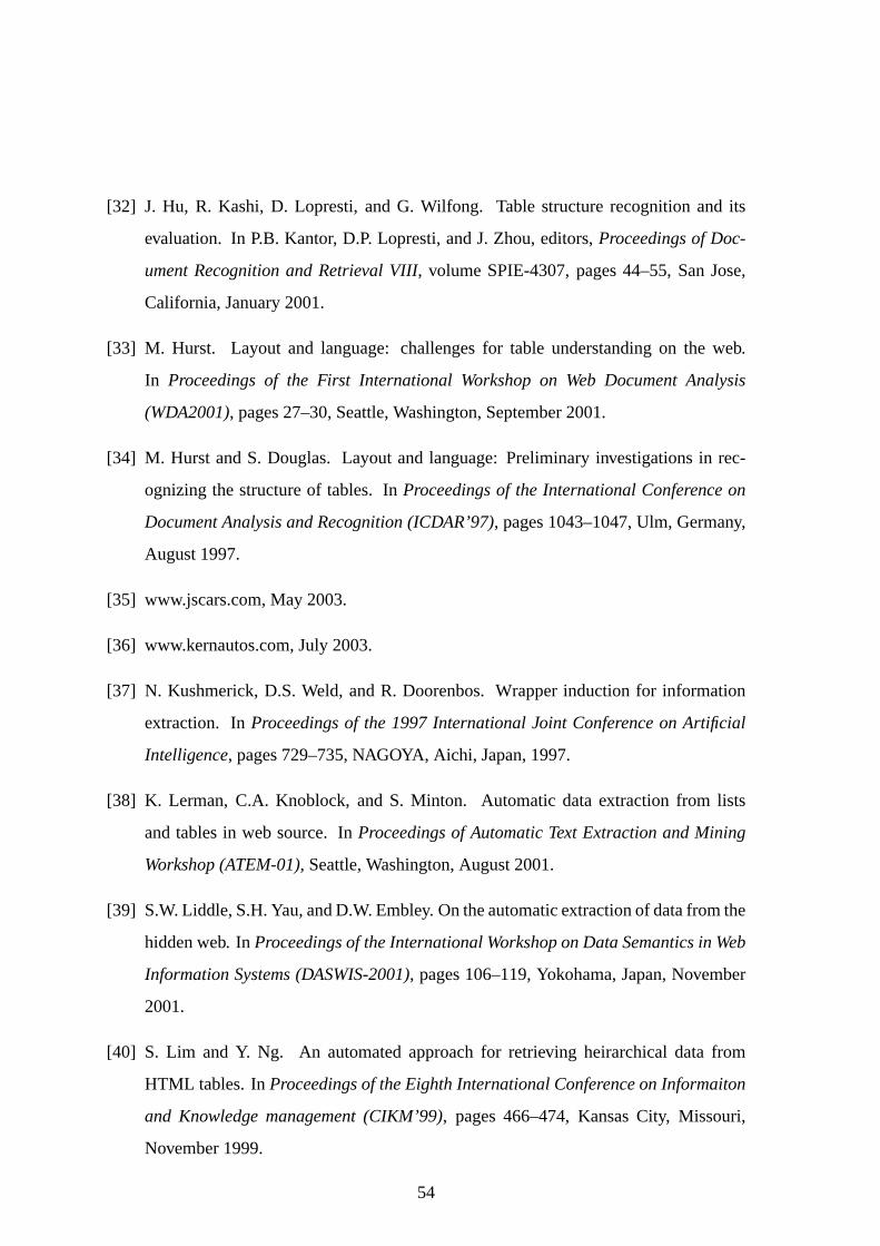
[32] J. Hu, R. Kashi, D. Lopresti, and G. Wilfong. Table structure recognition and its
evaluation. In P.B. Kantor, D.P. Lopresti, and J. Zhou, editors,Proceedings of Doc-
ument Recognition and Retrieval VIII, volume SPIE-4307, pages 44–55, San Jose,
California, January 2001.
[33] M. Hurst. Layout and language: challenges for table understanding on the web.
In Proceedings of the First International Workshop on Web Document Analysis
(WDA2001), pages 27–30, Seattle, Washington, September 2001.
[34] M. Hurst and S. Douglas. Layout and language: Preliminary investigations in rec-
ognizing the structure of tables. InProceedings of the International Conference on
Document Analysis and Recognition (ICDAR’97), pages 1043–1047, Ulm, Germany,
August 1997.
[35] www.jscars.com, May 2003.
[36] www.kernautos.com, July 2003.
[37] N. Kushmerick, D.S. Weld, and R. Doorenbos. Wrapper induction for information
extraction. InProceedings of the 1997 International Joint Conference on Artificial
Intelligence, pages 729–735, NAGOYA, Aichi, Japan, 1997.
[38] K. Lerman, C.A. Knoblock, and S. Minton. Automatic data extraction from lists
and tables in web source. InProceedings of Automatic Text Extraction and Mining
Workshop (ATEM-01), Seattle, Washington, August 2001.
[39] S.W. Liddle, S.H. Yau, and D.W. Embley. On the automatic extraction of data from the
hidden web. InProceedings of the International Workshop on Data Semantics in Web
Information Systems (DASWIS-2001), pages 106–119, Yokohama, Japan, November
2001.
[40] S. Lim and Y. Ng. An automated approach for retrieving heirarchical data from
HTML tables. InProceedings of the Eighth International Conference on Informaiton
and Knowledge management (CIKM’99), pages 466–474, Kansas City, Missouri,
November 1999.
54

[41] D. Lopresti and G. Nagy. Automated table processing: An (opinionated) survey. In
Proceedings of the Third IAPR Workshop on Graphics Recognition, pages 109–134,
Jaipur, India, September 1999.
[42] J. Madhavan, P.A. Bernstein, and E. Rahm. Generic schema matching with Cu-
pid. In Proceedings of the 27th International Conference on Very Large Data Bases
(VLDB’01), pages 49–58, Rome, Italy, September 2001.
[43] R. Miller, L. Haas, and M.A. Hernandez. Schema mapping as query discovery. InPro-
ceedings of the 26th International Conference on Very Large Databases (VLDB’00),
pages 77–88, Cairo, Egypt, September 2000.
[44] www.motorzones.com, July 2003.
[45] I. Muslea. Extraction patterns for information extraction tasks: survey. InProceedings
of American Association for Artificial Intelligence, pages 1–6, Orlando, Florida, July
1999.
[46] www.palmbeachclassifieds.com, July 2003.
[47] www.peakcellular.com, July 2003.
[48] P. Pyreddy and W.B. Croft. TINTIN: A system for retrieval in text tables. InProceed-
ings of the 2nd ACM International Conference on Digital Libraries, pages 193–200,
Philadelphia, Pennsylvania, July 1997.
[49] S. Raghavan and H. Garcia-Molina. Crawling the hidden web. InProceedings of the
27th International Conference on Very Large Data Bases (VLDB’01), Rome, Italy,
September 2001.
[50] S. Soderland. Learning information extraction rules for semi-structured and free text.
Machine Learning, 34(1–3):233–272, 1999.
[51] www.usedcars.com, July 2003.
55

[52] M. Yoshida, K. Torisawa, and J. Tsujii. A method to integrate tables of the world
wide web. InProceedings of the International Workshop on Web Document Analysis
(WDA 2001), pages 31–34, Washington, DC, September 2001.
56

Appendix
57

58

Appendix A
INTERESTING UNRESOLVED TABLES
59
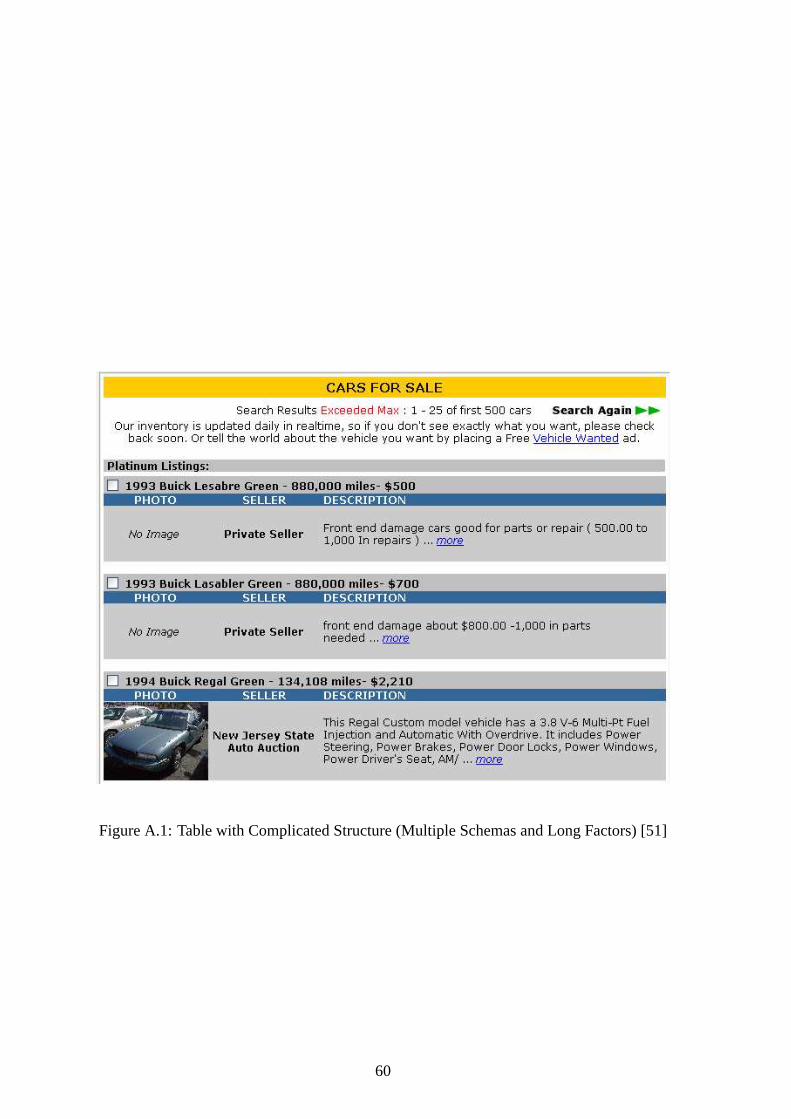
Figure A.1: Table with Complicated Structure (Multiple Schemas and Long Factors) [51]
60
Figure A.2: Table with Complicated Structure (Each Record Takes Multiple Rows) [6]
Figure A.3: Table with Complicated Schema (Attributes Take Multiple Rows) [46]
61
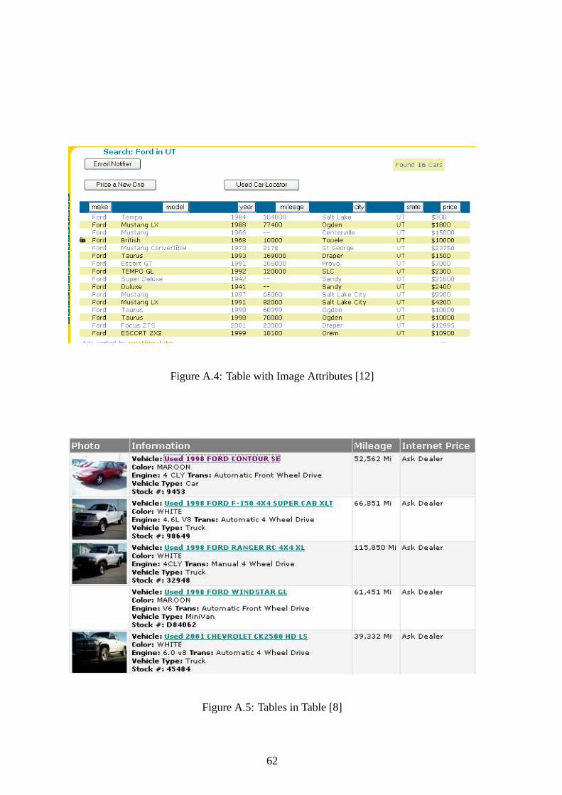
Figure A.4: Table with Image Attributes [12]
Figure A.5: Tables in Table [8]
62
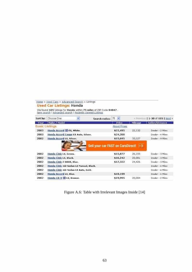
Figure A.6: Table with Irrelevant Images Inside [14]
63
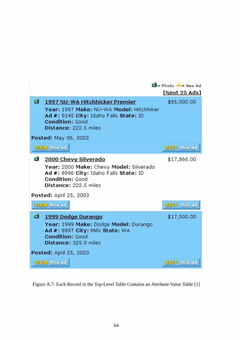
Figure A.7: Each Record in the Top-Level Table Contains an Attribute-Value Table [1]
64
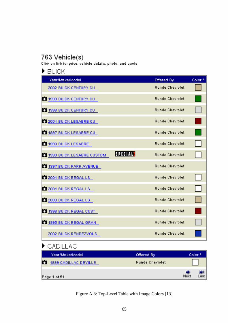
Figure A.8: Top-Level Table with Image Colors [13]
65
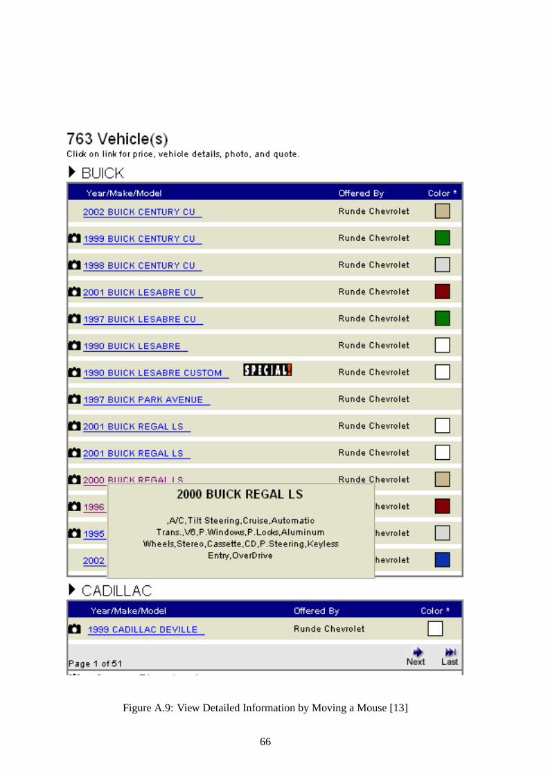
Figure A.9: View Detailed Information by Moving a Mouse [13]
66

Figure A.10: Top-Level Table with Complicated Structure [16]
Figure A.11: Top-Level Table with Only 2 Columns [4]
67
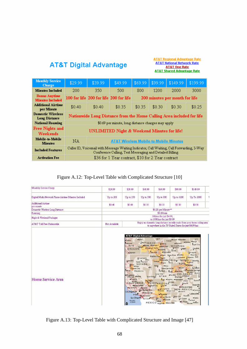
Figure A.12: Top-Level Table with Complicated Structure [10]
Figure A.13: Top-Level Table with Complicated Structure and Image [47]
68
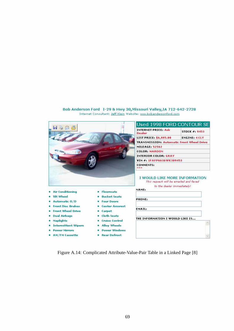
Figure A.14: Complicated Attribute-Value-Pair Table in a Linked Page [8]
69
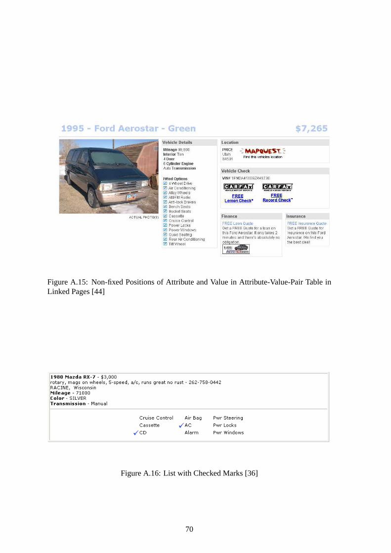
Figure A.15: Non-fixed Positions of Attribute and Value in Attribute-Value-Pair Table inLinked Pages [44]
Figure A.16: List with Checked Marks [36]
70
Related Documents