SCHEDULING SOURCES- Mark Manwaring Kia Bazargan Giovanni De Micheli Gupta Youn-Long Lin M. Balakrishnan Camposano, J. Hofstede, Knapp, MacMillen Lin.

SCHEDULINGSCHEDULINGSOURCES- Mark ManwaringKia BazarganGiovanni De Micheli GuptaYoun-Long Lin

M. BalakrishnanM. BalakrishnanCamposano, Camposano, J. Hofstede, J. Hofstede, Knapp,Knapp,MacMillenMacMillenLinLin

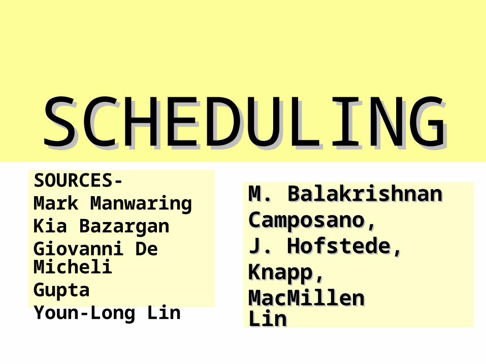
Overview of Hardware SynthesisOverview of Hardware Synthesis

assign times to operations under given constraints

reduce the amount of hardware, optimize the design in general.

May be done with the consideration of additional constraints.

assign operations to physical resources under given constraints

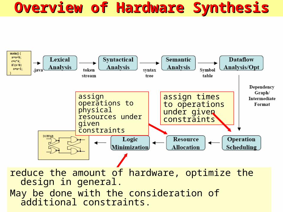
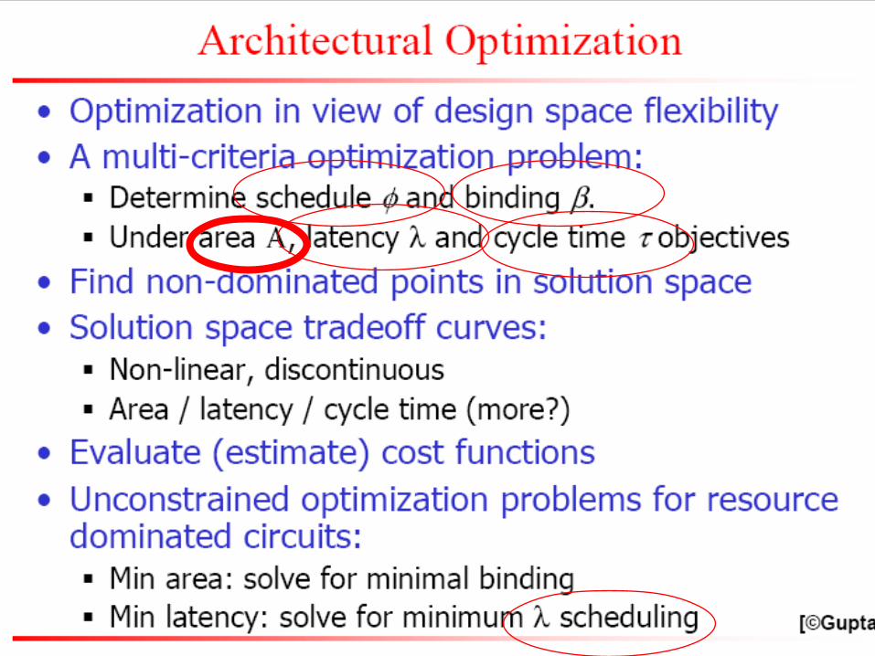
Outline of schedulingOutline of scheduling• The scheduling problem.

1. Scheduling without constraints.

2. Scheduling under timing constraints.• Relative scheduling.

3. Scheduling under resource constraints.• The ILP model (Integer Linear Programming).• Heuristic methods (graph coloring, etc).

Timing constraints versus resource constraintsresource constraints

What isWhat is SchedulingScheduling

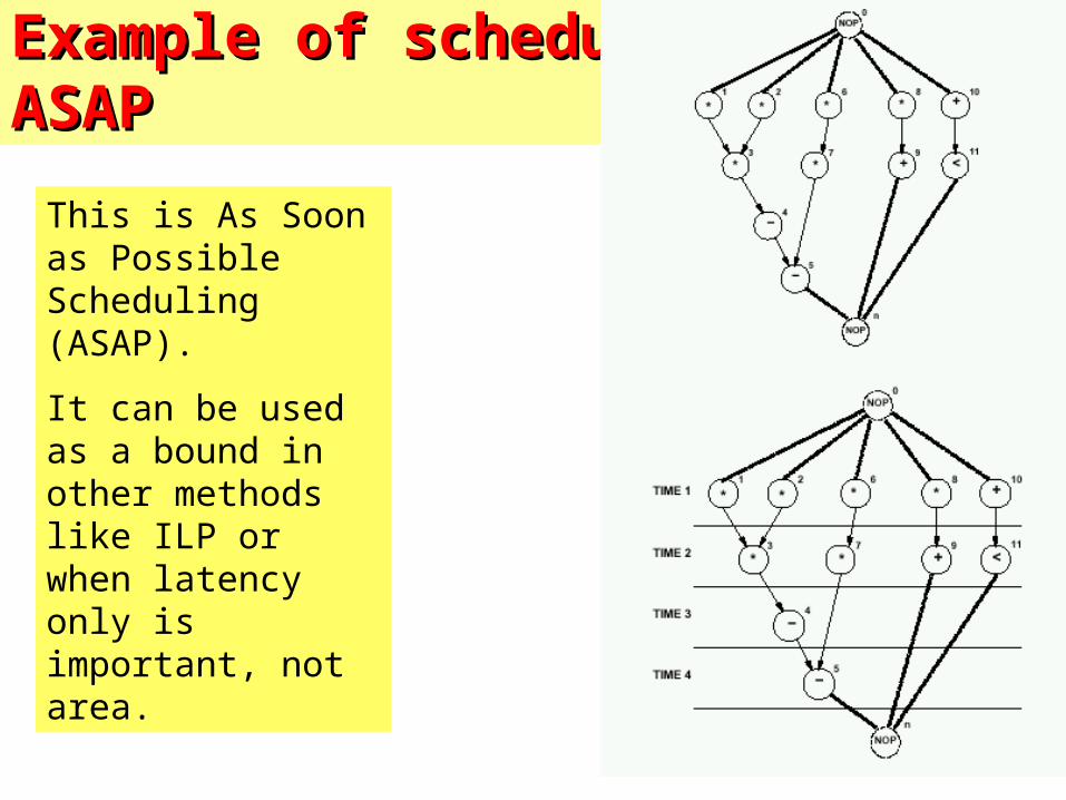
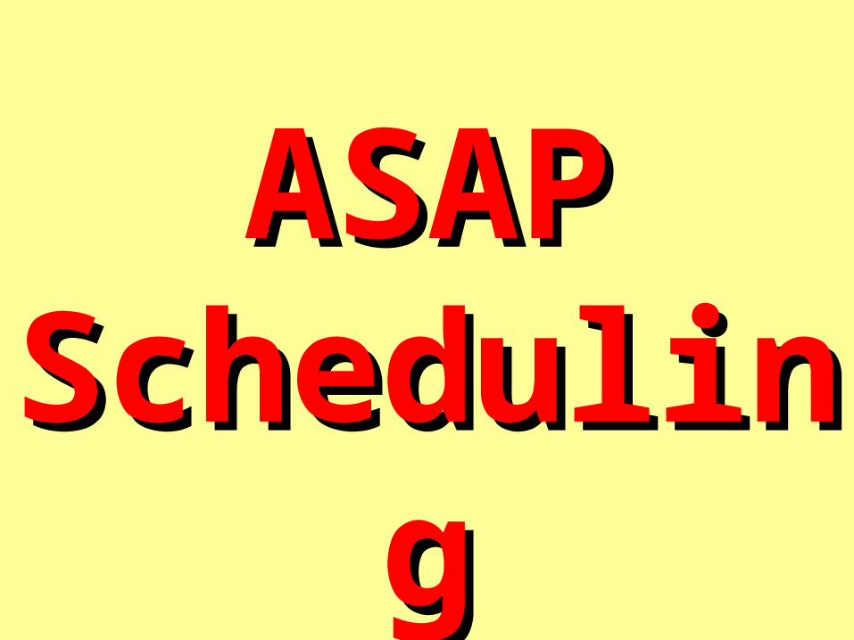
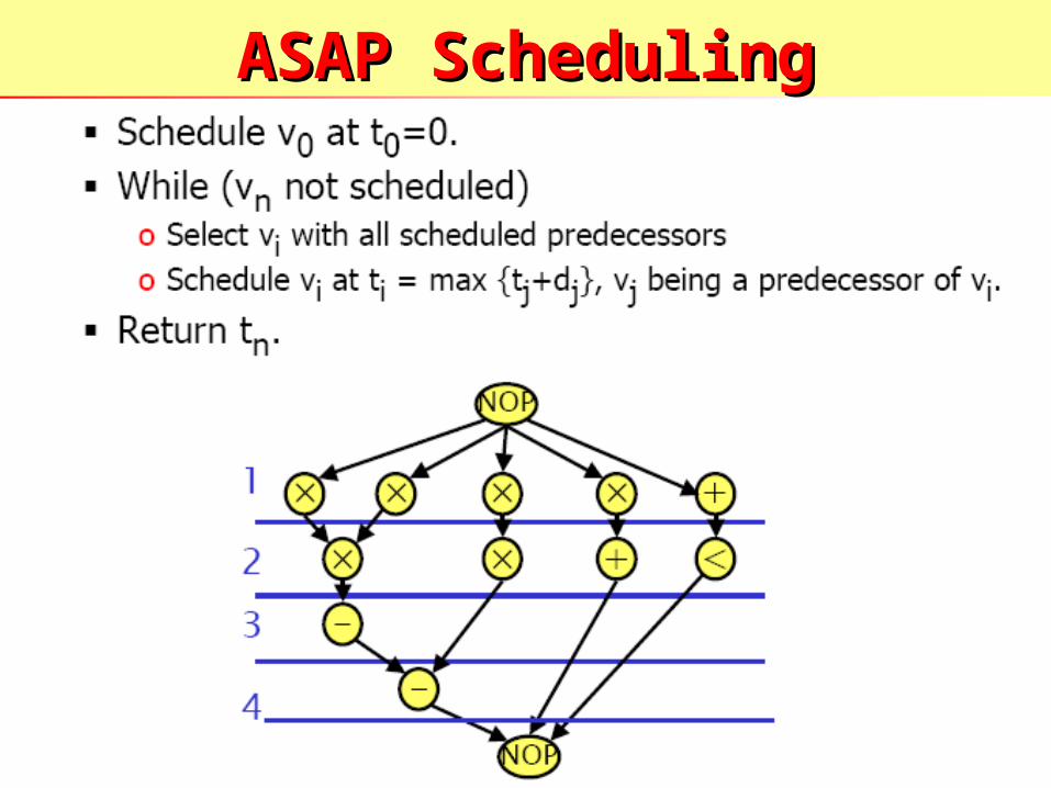
Example of scheduling:Example of scheduling:ASAPASAP

This is As Soon as Possible Scheduling (ASAP).

It can be used as a bound in other methods like ILP or when latency only is important, not area.

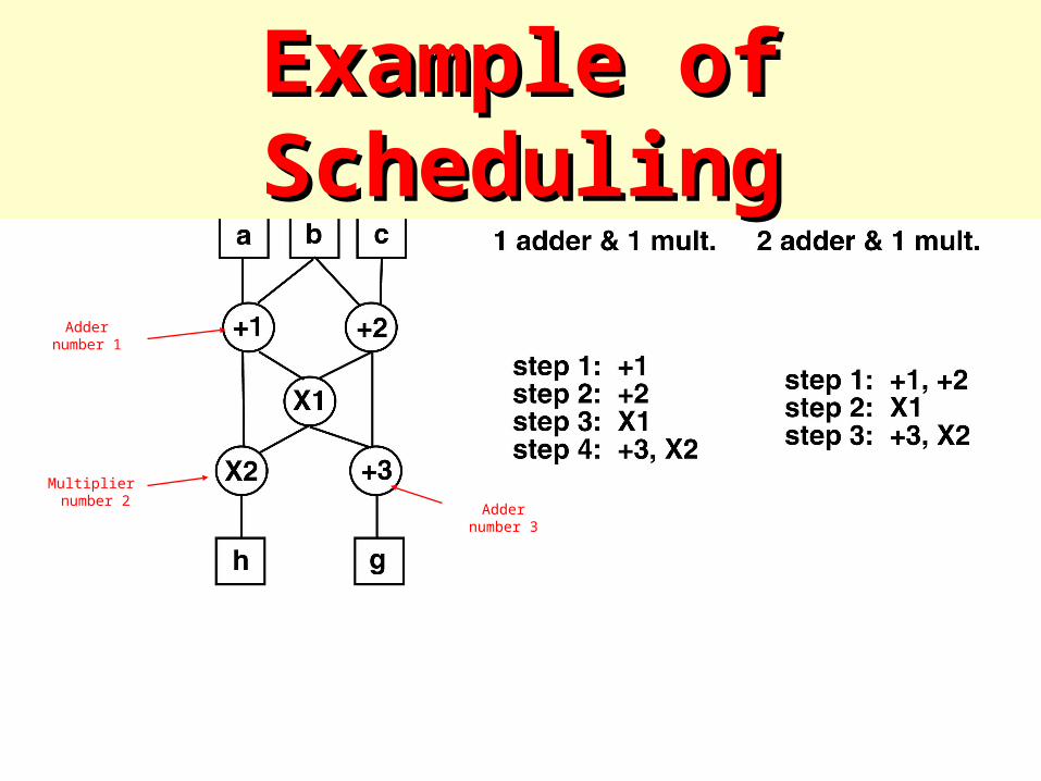
Example of SchedulingExample of Scheduling

Adder number 1

Adder number 3

Multiplier number 2

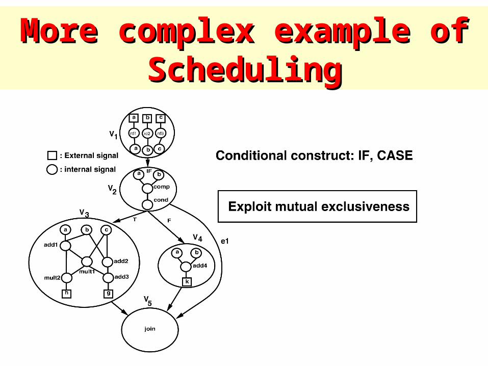
More complex example of More complex example of SchedulingScheduling

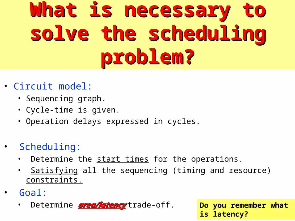
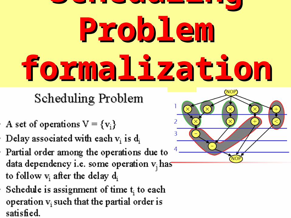
What is necessary to solve the What is necessary to solve the scheduling problem?scheduling problem?

• Circuit model:• Sequencing graph.• Cycle-time is given.• Operation delays expressed in cycles.

• Scheduling:• Determine the start times for the operations.• Satisfying all the sequencing (timing and resource) constraints.

• Goal:• Determine area/latencyarea/latency trade-off.

Do you remember what is latency?

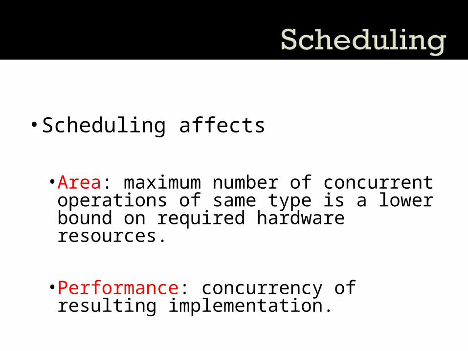
•Scheduling affects

•Area: maximum number of concurrent operations of same type is a lower bound on required hardware resources.

•Performance: concurrency of resulting implementation.

Taxonomy of scheduling Taxonomy of scheduling problems to solveproblems to solve

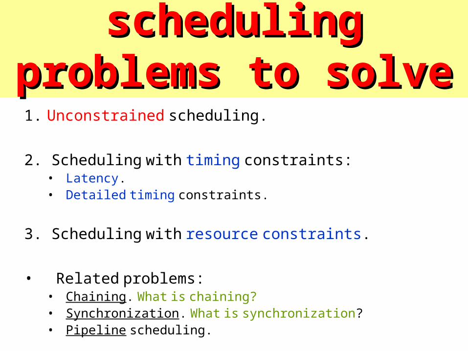
1. Unconstrained scheduling.

2. Scheduling with timing constraints:• Latency.• Detailed timing constraints.

3. Scheduling with resource constraints.

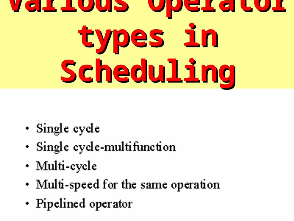
• Related problems:• Chaining. What is chaining?• Synchronization. What is synchronization?• Pipeline scheduling.

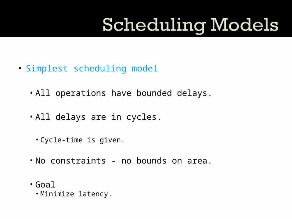
• Simplest scheduling model

• All operations have bounded delays.

• All delays are in cycles.

• Cycle-time is given.

• No constraints - no bounds on area.

• Goal• Minimize latency.

Scheduling 2Scheduling 2

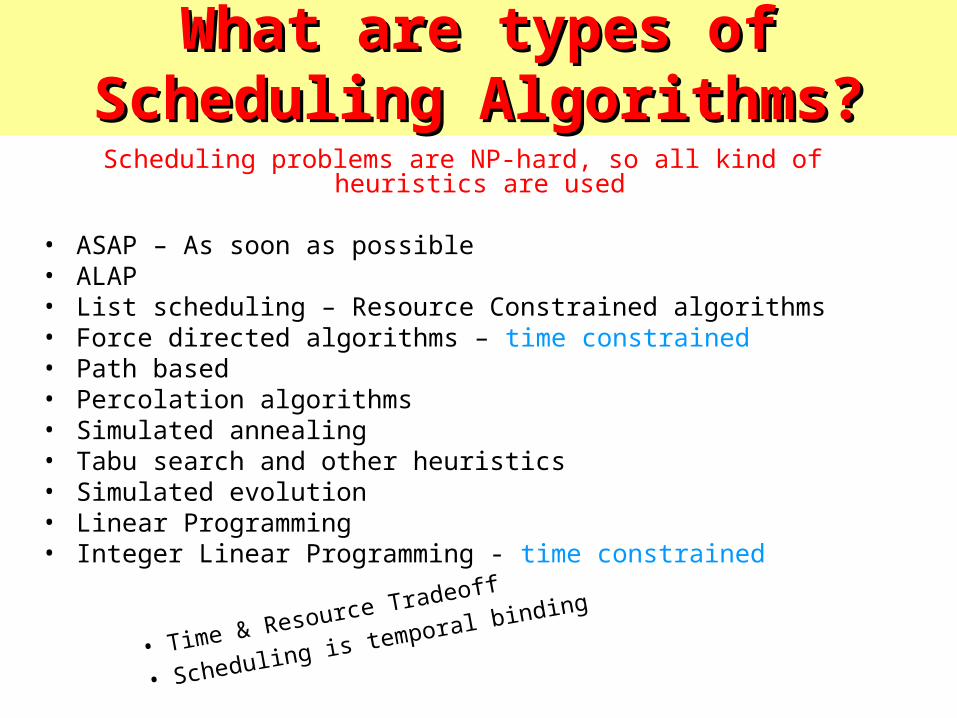
Scheduling problems are NP-hard, so all kind of heuristics are used

• ASAP – As soon as possible• ALAP• List scheduling – Resource Constrained algorithms• Force directed algorithms – time constrained• Path based• Percolation algorithms• Simulated annealing• Tabu search and other heuristics• Simulated evolution• Linear Programming• Integer Linear Programming - time constrained

What are types of Scheduling What are types of Scheduling Algorithms?Algorithms?

• Time & Resource Tradeoff

• Scheduling is temporal binding

Types of Scheduling ProcessesTypes of Scheduling Processes

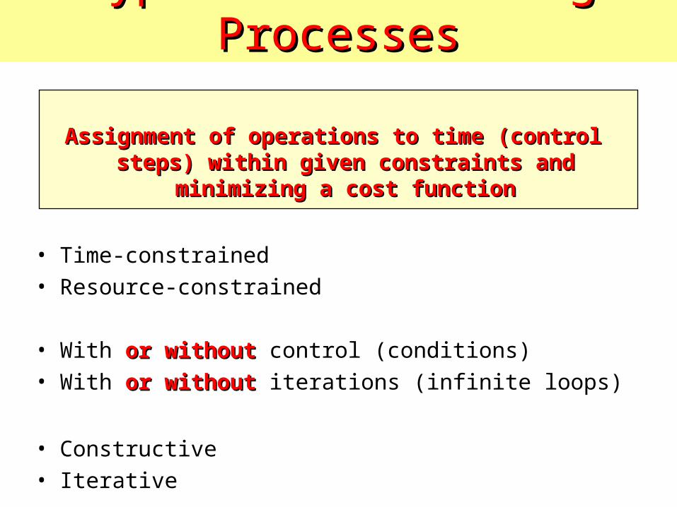
Assignment of operations to time (control Assignment of operations to time (control steps) within given constraints and steps) within given constraints and

minimizing a cost functionminimizing a cost function

• Time-constrained• Resource-constrained

• With or withoutor without control (conditions)• With or withoutor without iterations (infinite loops)

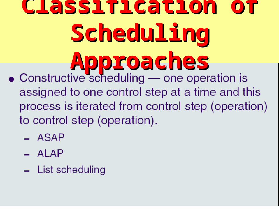
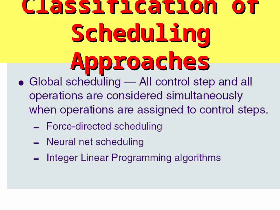
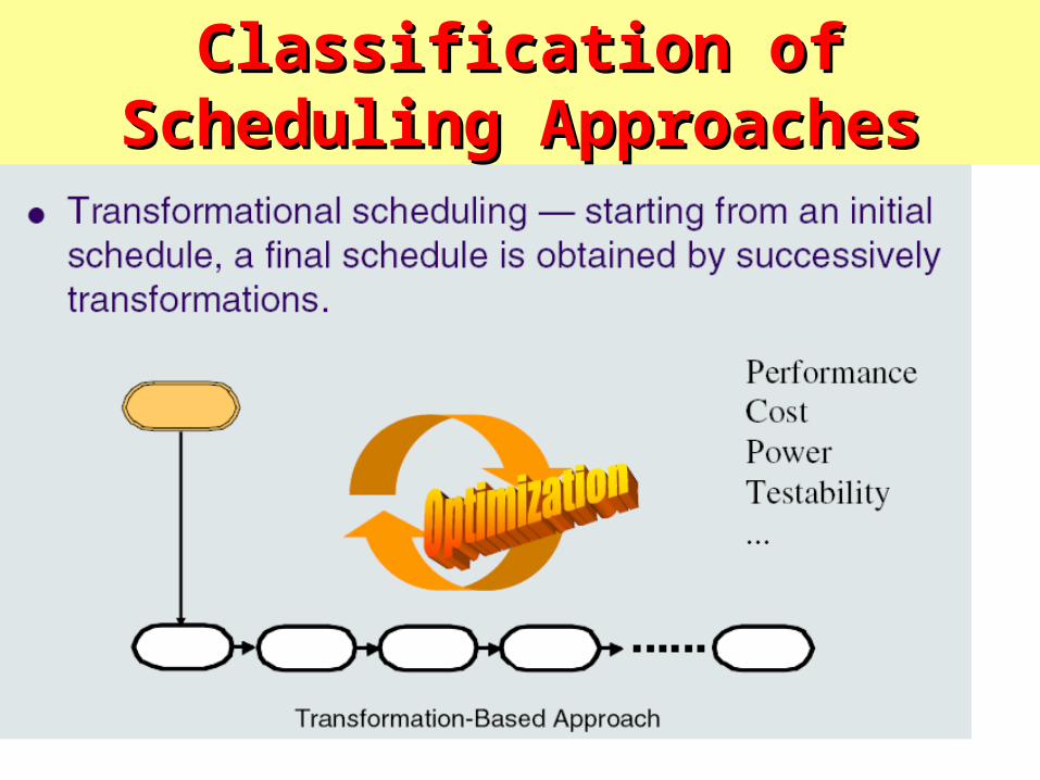
• Constructive• Iterative

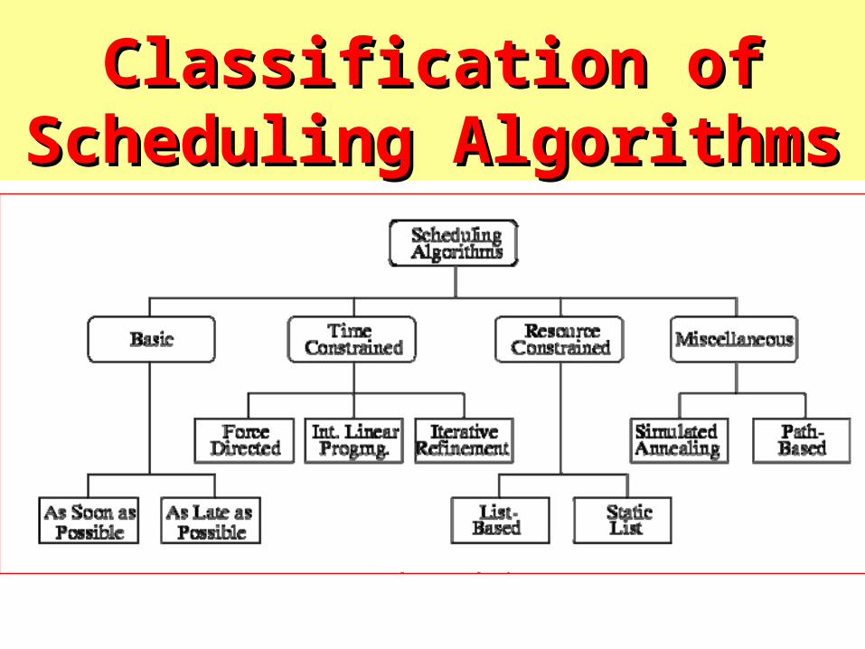
Classification of Scheduling Classification of Scheduling AlgorithmsAlgorithms

Scheduling Scheduling AlgorithmsAlgorithms

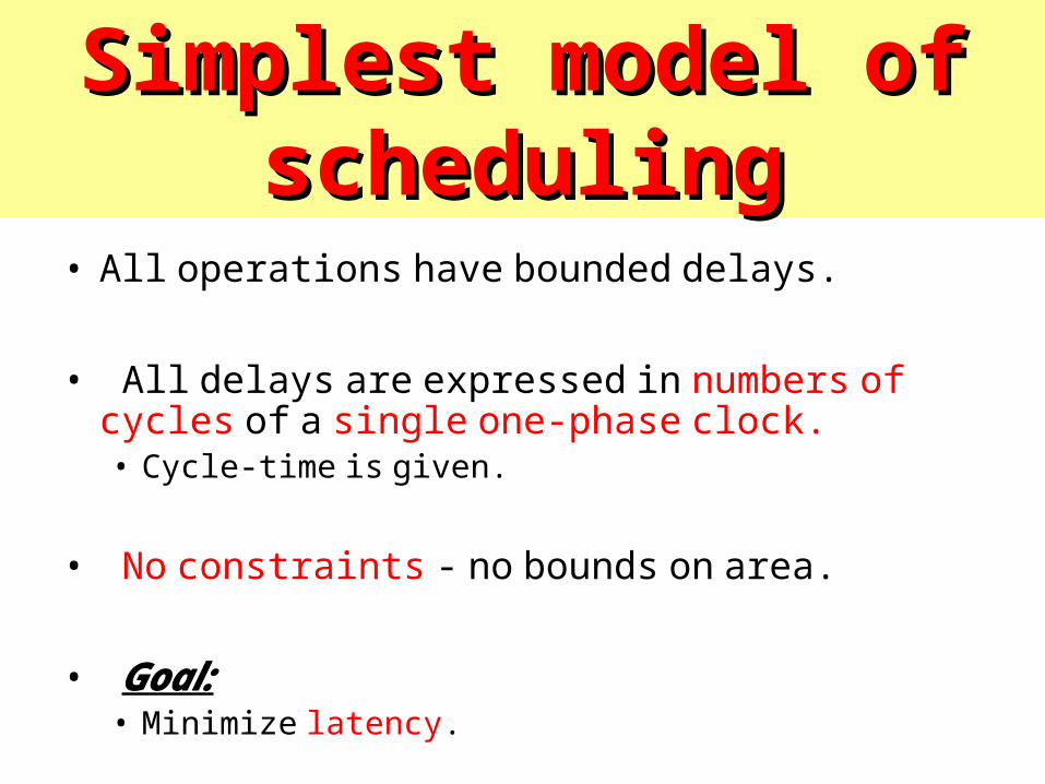
Simplest model of Simplest model of schedulingscheduling

• All operations have bounded delays.

• All delays are expressed in numbers of cycles of a single one-phase clock.• Cycle-time is given.

• No constraints - no bounds on area.

• Goal:• Minimize latency.

Minimum Latency Minimum Latency Unconstrained SchedulingUnconstrained Scheduling

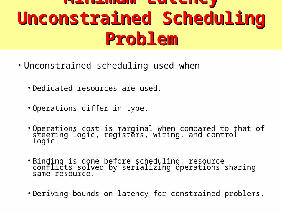
• Unconstrained scheduling used when

• Dedicated resources are used.

• Operations differ in type.

• Operations cost is marginal when compared to that of steering logic, registers, wiring, and control logic.

• Binding is done before scheduling: resource conflicts solved by serializing operations sharing same resource.

• Deriving bounds on latency for constrained problems.

Minimum Latency Unconstrained Minimum Latency Unconstrained Scheduling ProblemScheduling Problem

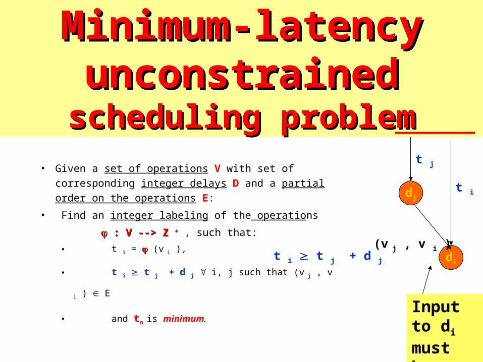
Minimum-latency Minimum-latency unconstrainedunconstrained

scheduling problemscheduling problem

• Given a set of operations V with set of corresponding integer delays D and a partial order on the operations E:

• Find an integer labeling of the operations

: V --> Z : V --> Z ++ , such that:

• t i = (v i ),

• t i t j + d j i, j such that (v j , v i ) E

• and tn is minimum.

di

dj

(v j , v i ) t i t j + d j

t j

t i

Input to di must be stable

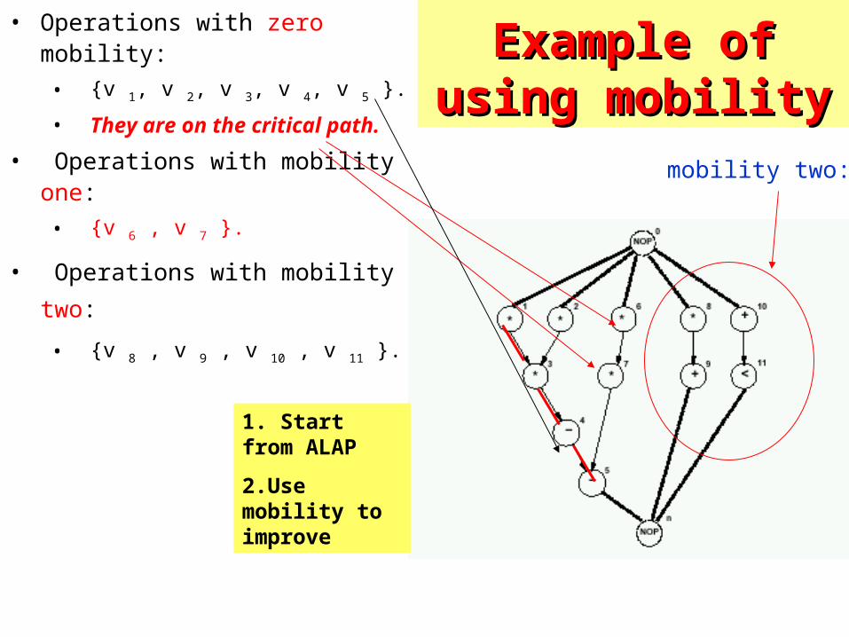
Example of using Example of using mobilitymobility

• Operations with zero mobility:

• {v 1, v 2, v 3, v 4, v 5 }.

• They are on the critical path.

• Operations with mobility one:

• {v 6 , v 7 }.

• Operations with mobility two:

• {v 8 , v 9 , v 10 , v 11 }.

mobility two:

1. Start from ALAP

2.Use mobility to improve

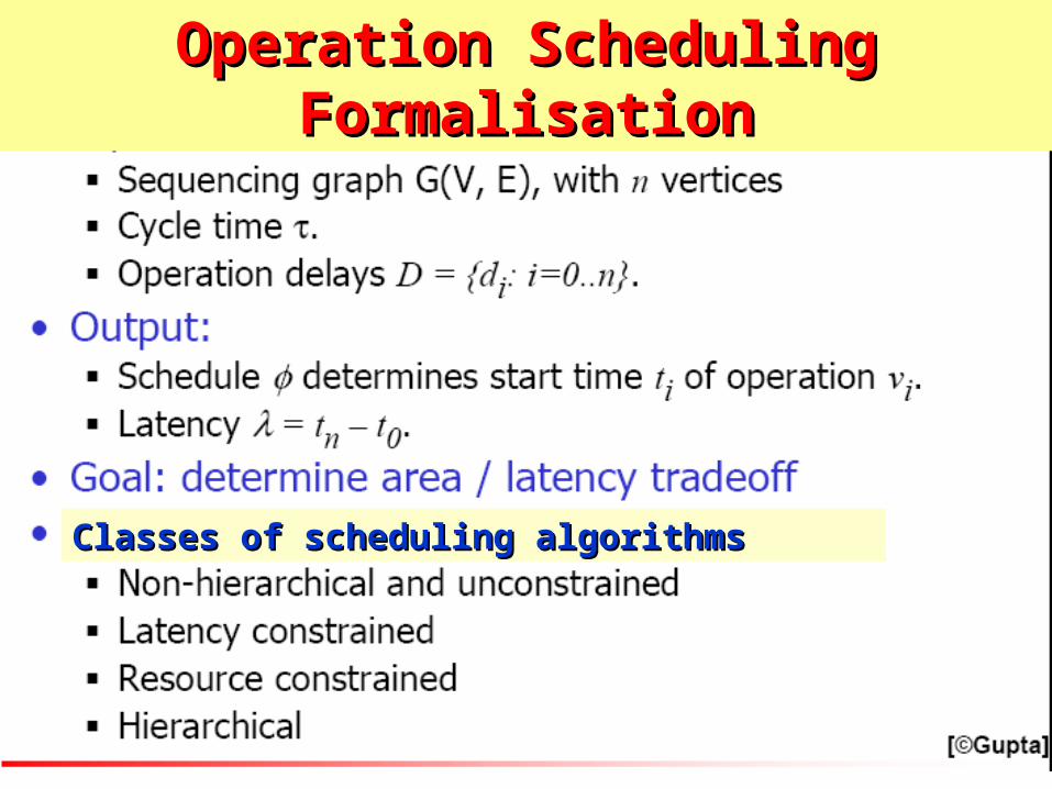
Classes of scheduling algorithmsClasses of scheduling algorithms

Operation Scheduling FormalisationOperation Scheduling Formalisation

Time Time Constrained Constrained SchedulingScheduling

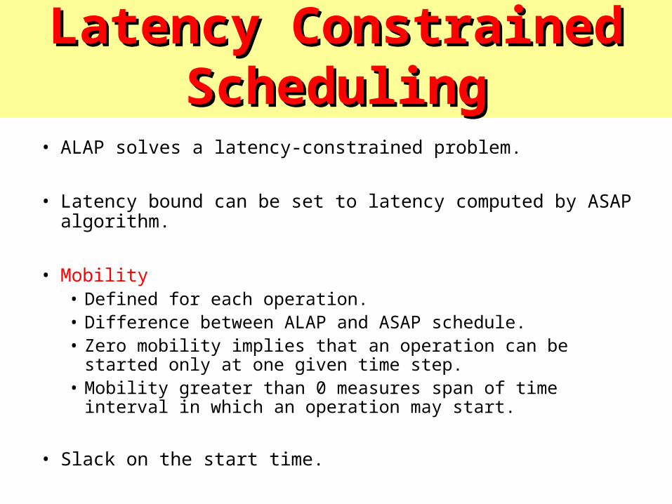
• ALAP solves a latency-constrained problem.

• Latency bound can be set to latency computed by ASAP algorithm.

• Mobility• Defined for each operation.• Difference between ALAP and ASAP schedule.• Zero mobility implies that an operation can be started

only at one given time step.• Mobility greater than 0 measures span of time interval in

which an operation may start.

• Slack on the start time.

Latency Constrained Latency Constrained SchedulingScheduling

Time Constrained Time Constrained SchedulingScheduling

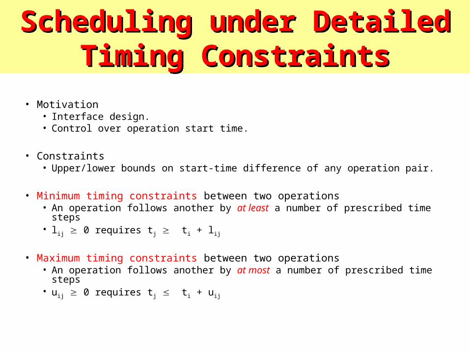
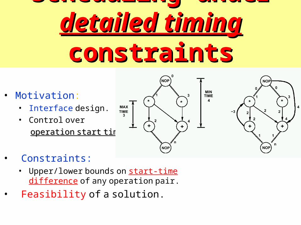
• Motivation• Interface design.• Control over operation start time.

• Constraints• Upper/lower bounds on start-time difference of any operation pair.

• Minimum timing constraints between two operations• An operation follows another by at least a number of prescribed time

steps• lij 0 requires tj ti + lij

• Maximum timing constraints between two operations• An operation follows another by at most a number of prescribed time

steps• uij 0 requires tj ti + uij

Scheduling under Detailed Scheduling under Detailed Timing ConstraintsTiming Constraints

• Example• Circuit reads data from a bus, performs computation, writes result

back on the bus.

• Bus interface constraint: data written three cycles after read.

• Minimum and maximum constraint of 3 cycles between read and write operations.

• Example• Two circuits required to communicate simultaneously to external

circuits.

• Cycle in which data available is irrelevant.

• Minimum and maximum timing constraint of zero cycles between two write operations.

Scheduling under Detailed Scheduling under Detailed Timing ConstraintsTiming Constraints

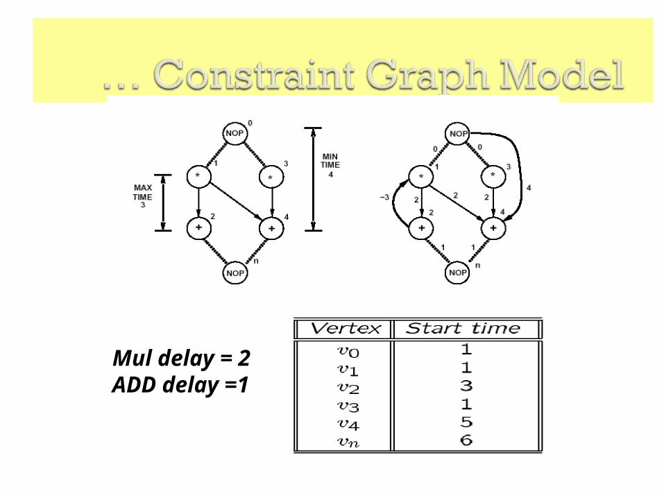
Mul delay = 2ADD delay =1

Scheduling under Scheduling under detailed detailed timing timing constraintsconstraints

• Motivation:• Interface design.• Control over

operation start timeoperation start time.

• Constraints:• Upper/lower bounds on start-time

difference of any operation pair.

• Feasibility of a solution.

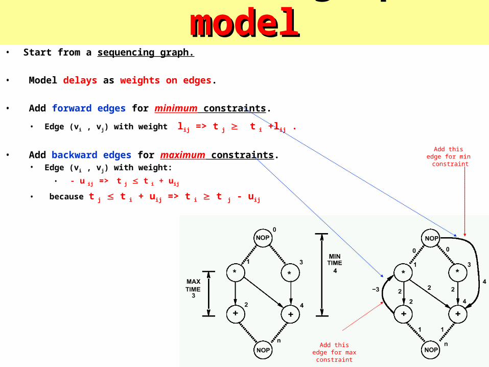
Constraint graph modelConstraint graph model• Start from a sequencing graph.

• Model delays as weights on edges.

• Add forward edges for minimum constraints.

• Edge (vi , vj) with weight lij => t j t i +lij .

• Add backward edges for maximum constraints.• Edge (vi , vj) with weight:

• - u ij => t j t i + uij

• because t j t i + uij => t i t j - uij

Add this edge for max constraint

Add this edge for min constraint

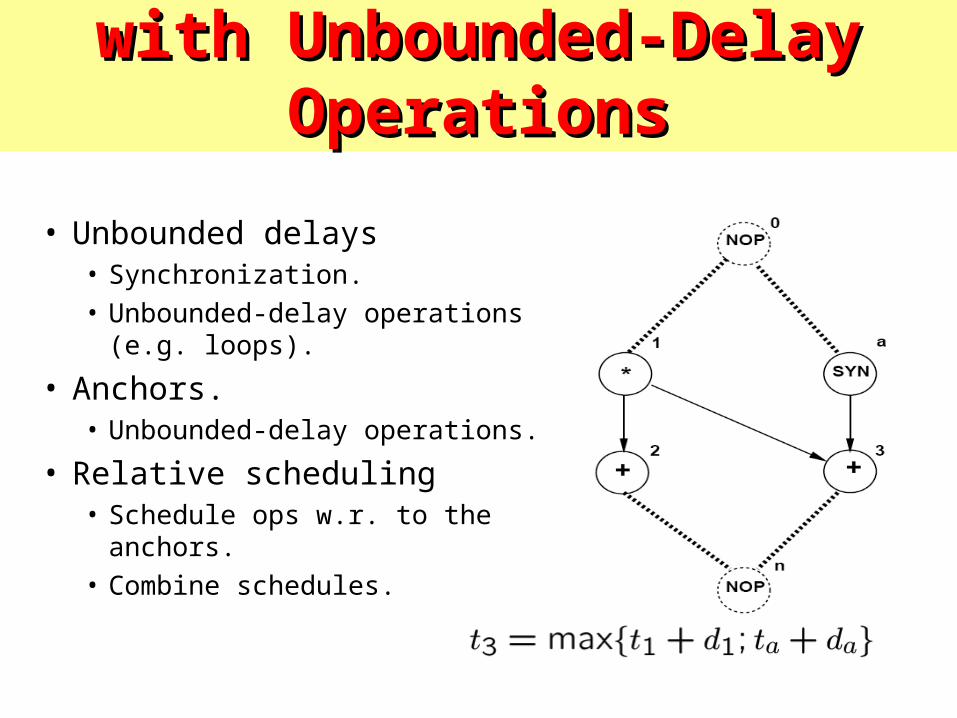
• Unbounded delays• Synchronization.• Unbounded-delay operations (e.g.

loops).

• Anchors.• Unbounded-delay operations.

• Relative scheduling• Schedule ops w.r. to the anchors.• Combine schedules.

Method for Scheduling with Method for Scheduling with Unbounded-Delay OperationsUnbounded-Delay Operations

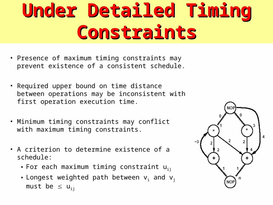
• Presence of maximum timing constraints may prevent existence of a consistent schedule.

• Required upper bound on time distance between operations may be inconsistent with first operation execution time.

• Minimum timing constraints may conflict with maximum timing constraints.

• A criterion to determine existence of a schedule:

• For each maximum timing constraint uij

• Longest weighted path between vi and vj must be uij

Method for Scheduling Under Method for Scheduling Under Detailed Timing ConstraintsDetailed Timing Constraints

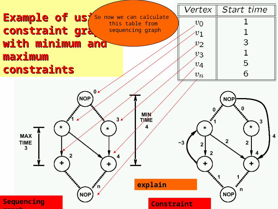
Example of using Example of using constraint graph with constraint graph with minimum and maximum minimum and maximum constraintsconstraints

Sequencing graph Constraint graph

explain

So now we can calculate this table from

sequencing graph

• Weight of longest path from source to a vertex is the minimum start time of a vertex.

• Bellman-Ford or Lia-Wong algorithm provides the schedule.

• A necessary condition for existence of a schedule is constraint graph has no positive cycles.

Method for Scheduling Under Method for Scheduling Under Detailed Timing ConstraintsDetailed Timing Constraints

Methods for Scheduling Methods for Scheduling Under Detailed Timing Under Detailed Timing

ConstraintsConstraints

Shown in last slide

Will follow

Methods for schedulingMethods for schedulingunder under detailed timingdetailed timing constraints constraints• Start from the Sequencing Graph. Assumption:

• All delays are fixed and known.

• Set of linear inequalities.

• Longest path problem.

• Algorithms for the longest path problemlongest path problem were discussed in Chapter 2 of De Micheli:• Bellman-Ford,Bellman-Ford,• Liao-Wong.Liao-Wong.

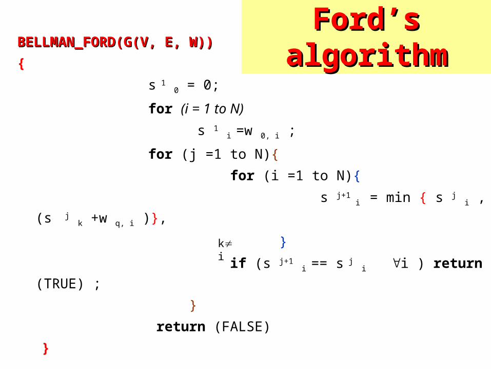
Bellman-Ford’s Bellman-Ford’s algorithmalgorithm

BELLMAN_FORD(G(V, E, W))BELLMAN_FORD(G(V, E, W))

{

s 1 0 = 0;

for (i = 1 to N)

s 1 i =w 0, i ;

for (j =1 to N){

for (i =1 to N){

s j+1 i = min { s j i , (s j k +w q, i )},

}

if (s j+1 i == s j i i ) return (TRUE) ;

}

return (FALSE)

}

ki

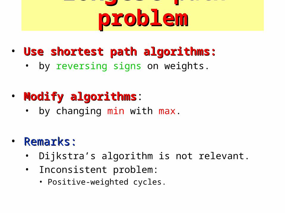
LongestLongest path problem path problem

• Use shortest path algorithms:Use shortest path algorithms:• by reversing signs on weights.

• Modify algorithmsModify algorithms:• by changing min with max.

• Remarks:Remarks:• Dijkstra’s algorithm is not relevant.• Inconsistent problem:

• Positive-weighted cycles.

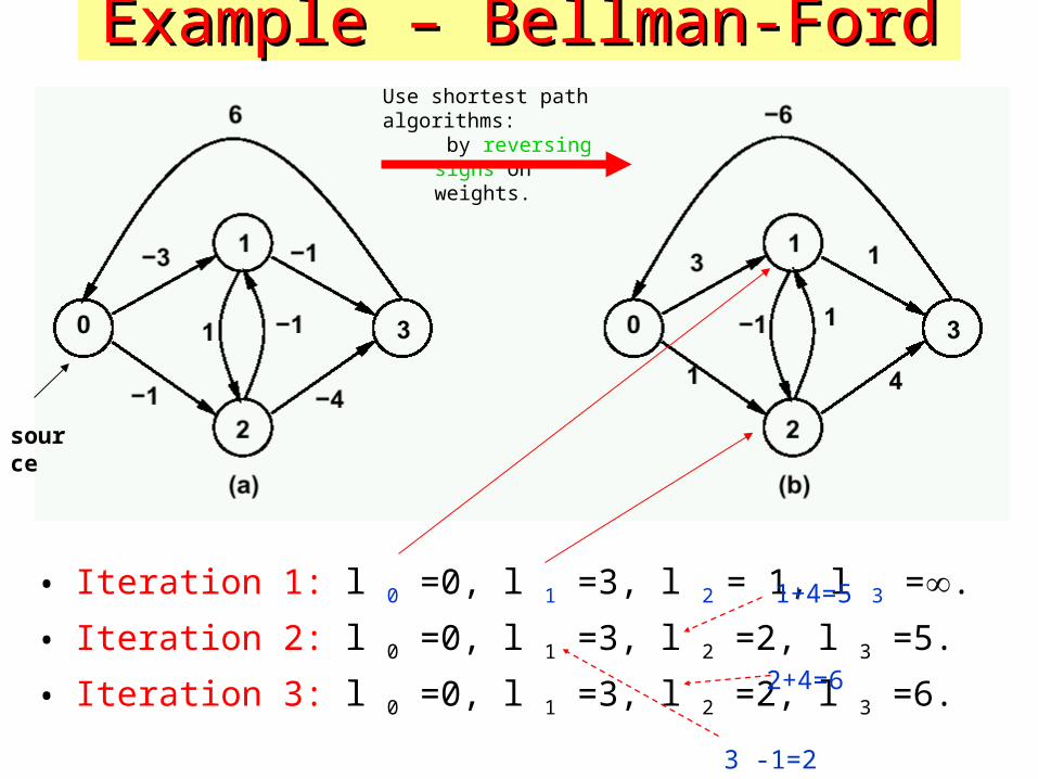
Example – Bellman-FordExample – Bellman-Ford

• Iteration 1: l 0 =0, l 1 =3, l 2 = 1, l 3 =.

• Iteration 2: l 0 =0, l 1 =3, l 2 =2, l 3 =5.

• Iteration 3: l 0 =0, l 1 =3, l 2 =2, l 3 =6.

Use shortest path algorithms: by reversing signs on weights.

source

3 -1=2

1+4=5

2+4=6

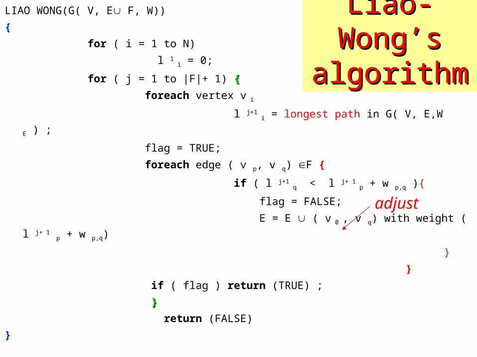
Liao-Wong’s Liao-Wong’s algorithmalgorithm

LIAO WONG(G( V, E F, W))

{

for ( i = 1 to N)

l 1 i = 0;

for ( j = 1 to |F|+ 1) {{

foreach vertex v i

l j+1 i = longest path in G( V, E,W E ) ;

flag = TRUE;

foreach edge ( v p, v q) F {

if ( l j+1 q < l j+ 1

p + w p,q ){

flag = FALSE;

E = E ( v 0 , v q) with weight ( l j+ 1 p + w p,q)

}

}

if ( flag ) return (TRUE) ;

}}

return (FALSE)

}

adjust

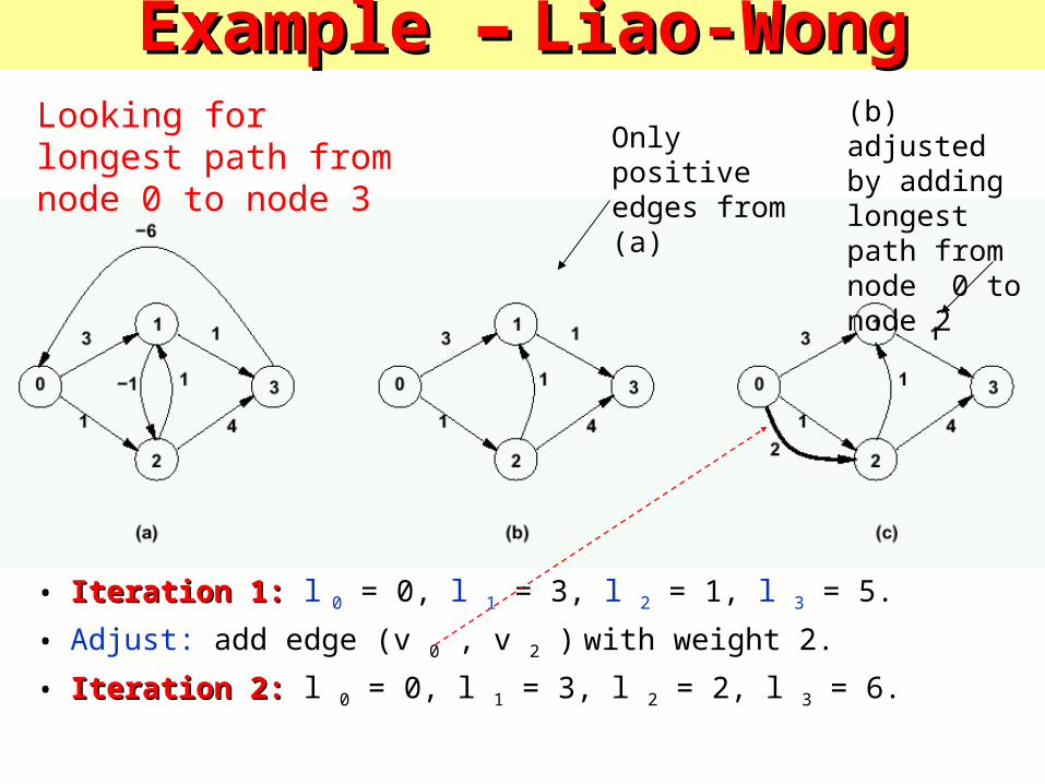
Example Example – – Liao-WongLiao-Wong

• Iteration 1:Iteration 1: l 0 = 0, l 1 = 3, l 2 = 1, l 3 = 5.

• Adjust: add edge (v 0 , v 2 ) with weight 2.

• Iteration 2:Iteration 2: l 0 = 0, l 1 = 3, l 2 = 2, l 3 = 6.

Only positive edges from (a)

(b) adjusted by adding longest path from node 0 to node 2

Looking for longest path from node 0 to node 3

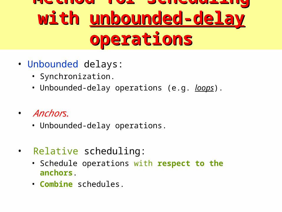
Method for schedulingMethod for schedulingwith with unbounded-delayunbounded-delay operations operations• Unbounded delays:

• Synchronization.• Unbounded-delay operations (e.g. loops).

• Anchors.• Unbounded-delay operations.

• Relative scheduling:• Schedule operations with respect to the anchors.• Combine schedules.

Relative Relative scheduling scheduling

methodmethod

Relative scheduling Relative scheduling methodmethod

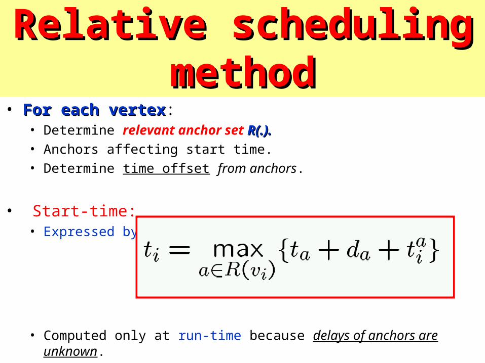
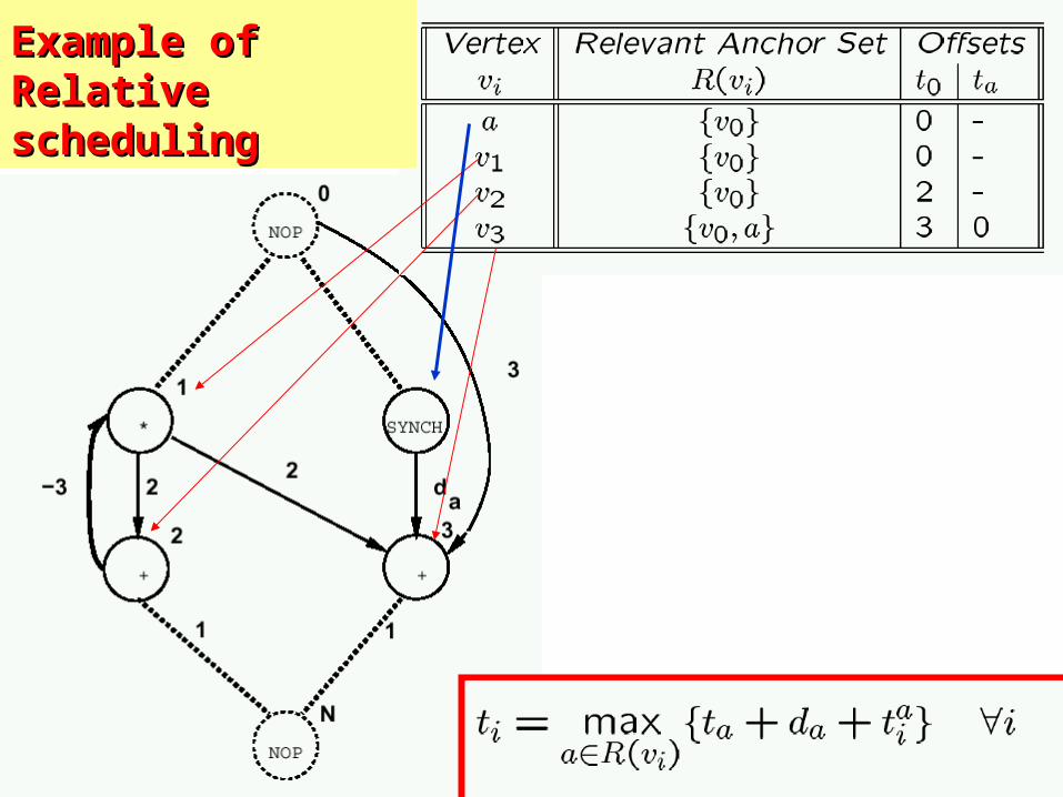
• For each vertexFor each vertex:• Determine relevant anchor set R(.).R(.).• Anchors affecting start time.• Determine time offset from anchors.

• Start-time:• Expressed by:

• Computed only at run-time because delays of anchors are unknown.

Relative scheduling under Relative scheduling under timingtimingconstraintsconstraints

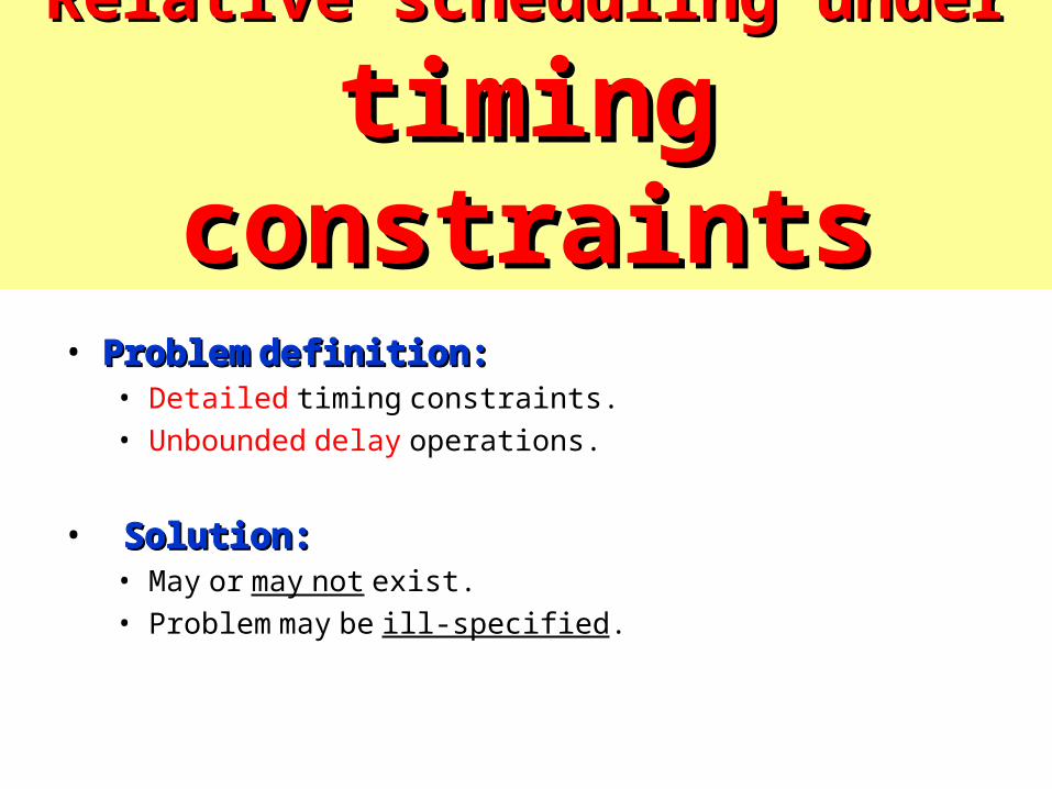
• Problem definition:Problem definition:• Detailed timing constraints.• Unbounded delay operations.

• Solution:Solution:• May or may not exist.• Problem may be ill-specified.

Relative scheduling Relative scheduling under timingunder timingconstraintsconstraints

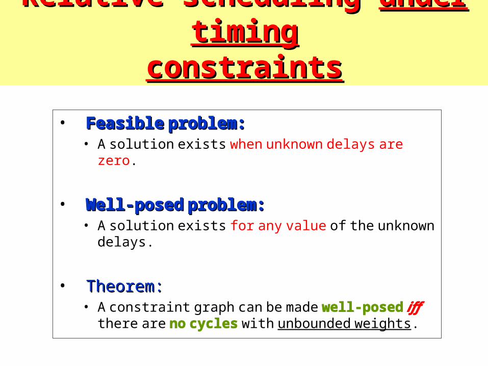
• Feasible problem:Feasible problem:• A solution exists when unknown delays are zero.

• Well-posed problem:Well-posed problem:• A solution exists for any value of the unknown delays.

• Theorem:Theorem:• A constraint graph can be made well-posed iff there

are no cycles with unbounded weights.

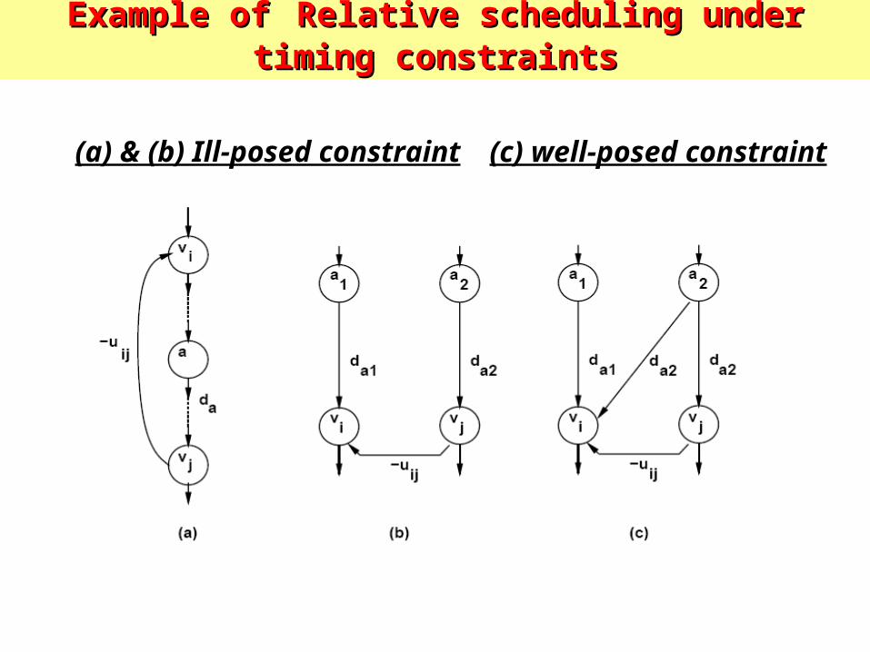
(a) & (b) Ill-posed constraint (c) well-posed constraint

Example ofExample of Relative scheduling under timing constraintsRelative scheduling under timing constraints

Relative scheduling approachRelative scheduling approach

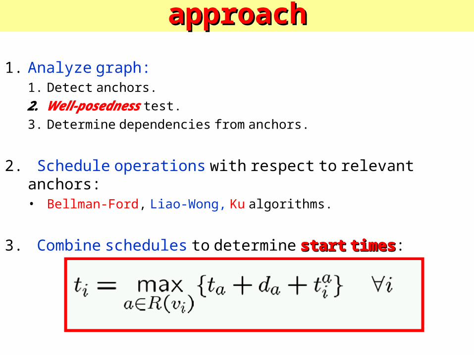
1. Analyze graph:1. Detect anchors.

2. Well-posedness test.

3. Determine dependencies from anchors.

2. Schedule operations with respect to relevant anchors:• Bellman-Ford, Liao-Wong, Ku algorithms.

3. Combine schedules to determine start timesstart times:

Example of Relative Example of Relative scheduling scheduling

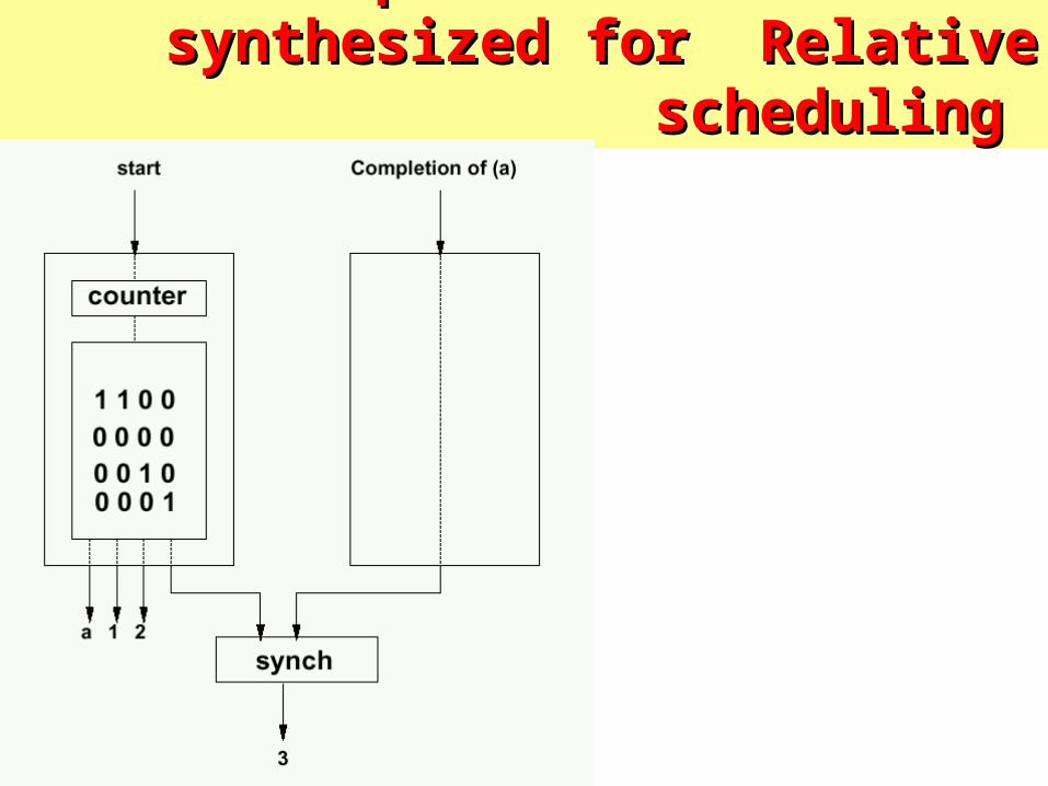
Example of control-unit synthesized for Example of control-unit synthesized for Relative scheduling Relative scheduling

Operations must be serialized

Scheduling and BindingScheduling and Binding

schedule binding

Scheduling Scheduling ProblemProblemScheduling Problem Scheduling Problem

formalizationformalization

Various Operator Various Operator types in Schedulingtypes in Scheduling

ASAP ASAP SchedulingScheduling

ASAP SchedulingASAP Scheduling

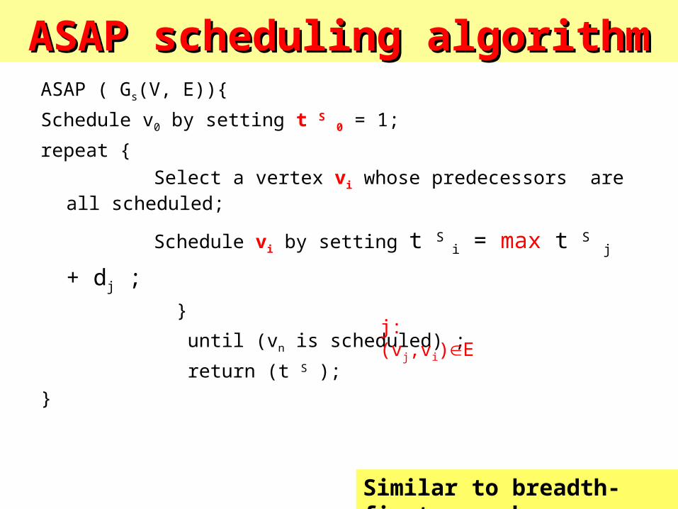
ASAP scheduling algorithmASAP scheduling algorithmASAP ( Gs(V, E)){

Schedule v0 by setting t S 0 = 1;

repeat { Select a vertex vi whose predecessors are all

scheduled;

Schedule vi by setting t S i = max t S j + dj ;

}

until (vn is scheduled) ;

return (t S );}

j:(vj,vi)E

Similar to breadth-first search

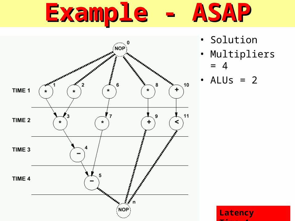
Example - ASAPExample - ASAP• Solution• Multipliers =

4• ALUs = 2

Latency Time=4

ALAP ALAP SchedulingScheduling

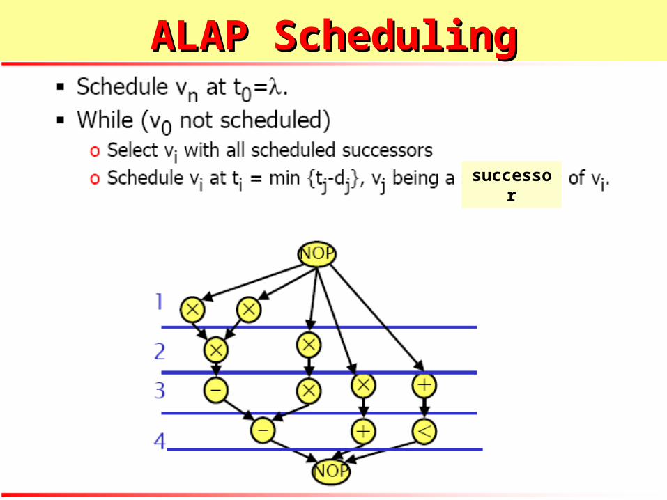
ALAP SchedulingALAP Scheduling

successor

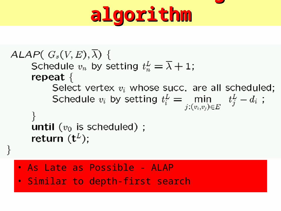
ALAP scheduling algorithmALAP scheduling algorithm

• As Late as Possible - ALAP• Similar to depth-first search

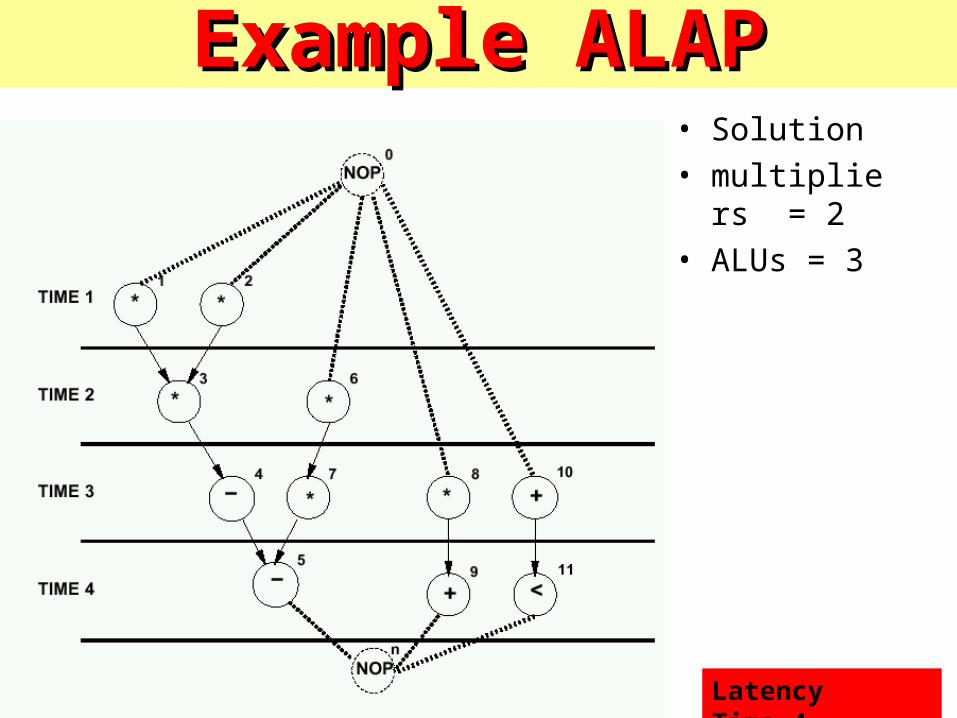
Example ALAPExample ALAP• Solution• multipliers

= 2• ALUs = 3

Latency Time=4

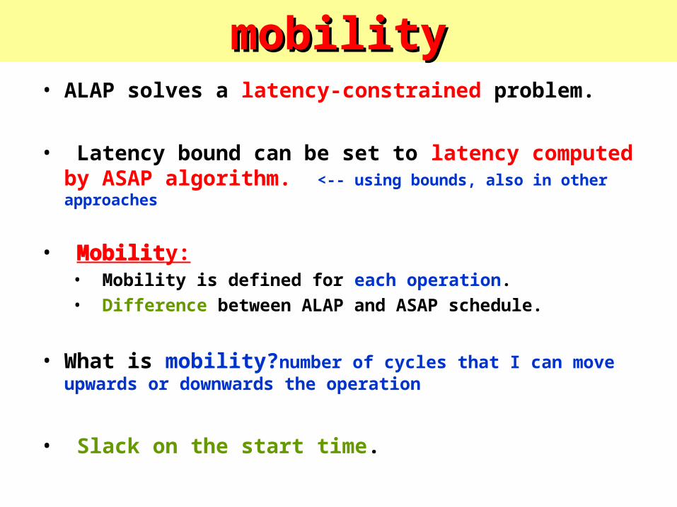
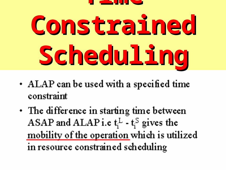
Remarks on ALAP and mobilityRemarks on ALAP and mobility• ALAP solves a latency-constrained problem.

• Latency bound can be set to latency computed by ASAP algorithm. <-- using bounds, also in other approaches

• Mobility:• Mobility is defined for each operation.• Difference between ALAP and ASAP schedule.

• What is mobility?number of cycles that I can move upwards or downwards the operation

• Slack on the start time.

Resource Resource ConstrainedConstrained

Scheduling under Scheduling under

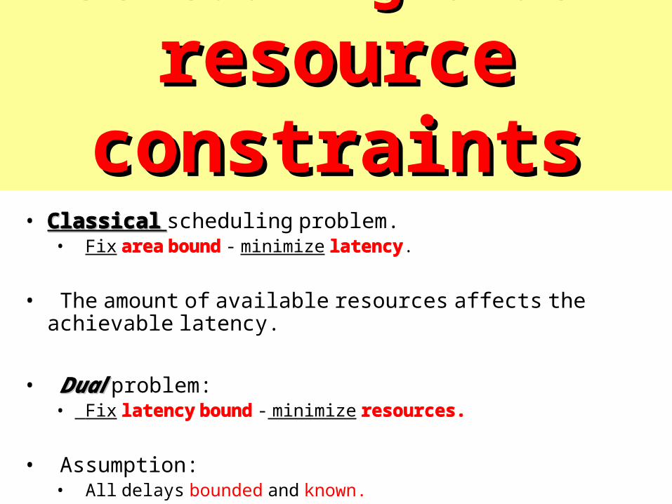
resource constraintsresource constraints• Classical Classical scheduling problem.

• Fix area bound - minimize latency.

• The amount of available resources affects the achievable latency.

• DualDual problem:• Fix latency bound - minimize resources.

• Assumption:• All delays bounded and known.

Minimum latencyMinimum latency resource-constrained resource-constrainedscheduling problemscheduling problem

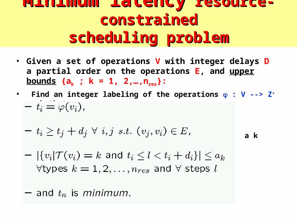
• Given a set of operations V with integer delays D a partial order on the operations E, and upper bounds {ak ; k = 1, 2,…,nres}:

• Find an integer labeling of the operations : V --> Z+ such that :• t i = '(v i ),• t i t j +d j 8 i; j s:t: (v j ; v i ) 2 E,• jfv i jT (v i ) = k and t i l < t i +d i gj a k• and tn is minimum.

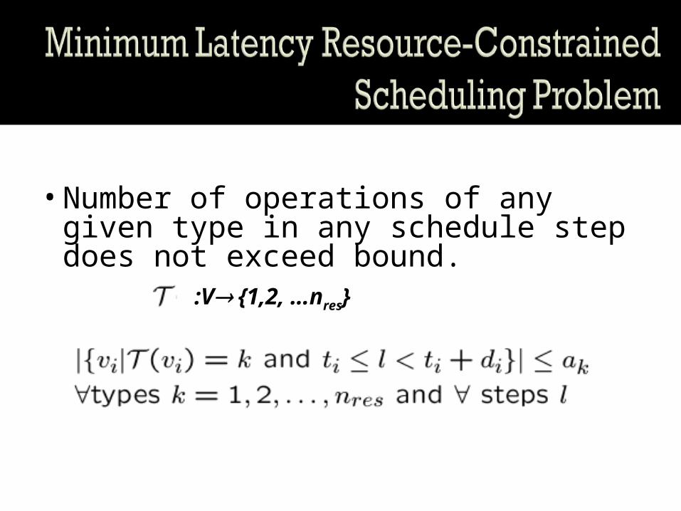
•Number of operations of any given type in any schedule step does not exceed bound.

:V {1,2, …nres}

Scheduling under Scheduling under resource resource constraintsconstraints

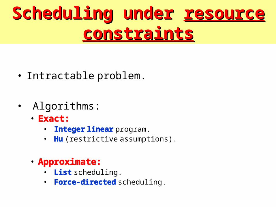
• Intractable problem.

• Algorithms:• Exact:

• Integer linear program.• Hu (restrictive assumptions).

• Approximate:• List scheduling.• Force-directed scheduling.

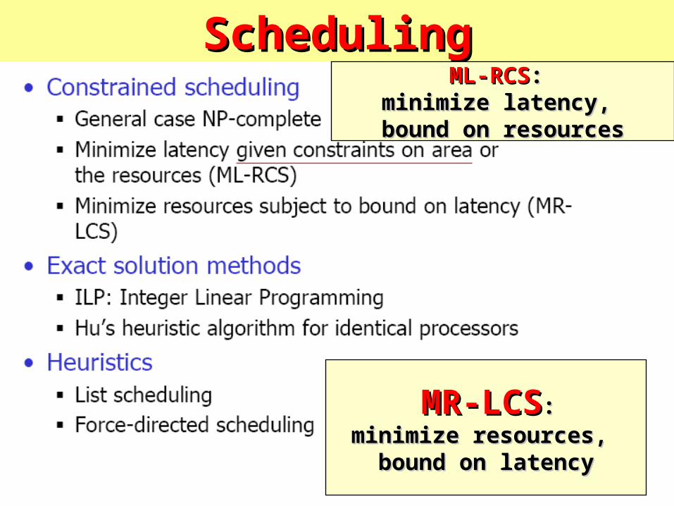
Resource Constraint SchedulingResource Constraint SchedulingML-RCSML-RCS: :

minimize latency, minimize latency, bound on resourcesbound on resources

MR-LCSMR-LCS: : minimize resources, minimize resources,

bound on latencybound on latency

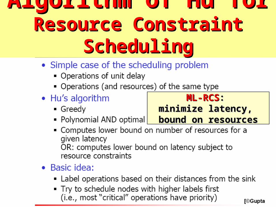
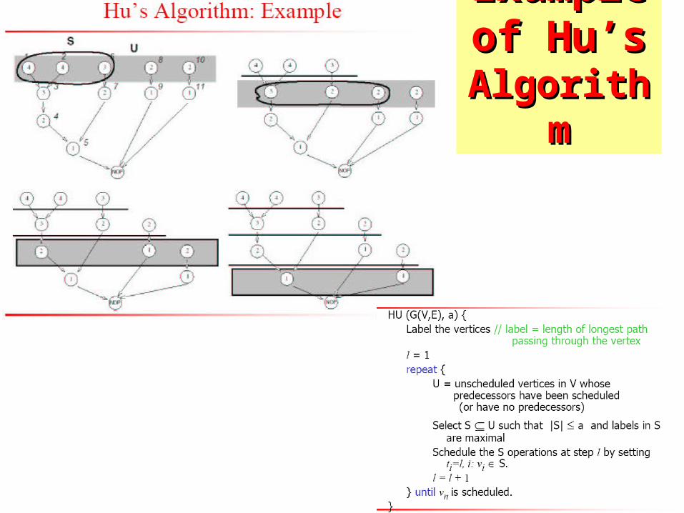
Algorithm of Hu for Algorithm of Hu for Resource Constraint SchedulingResource Constraint Scheduling

ML-RCSML-RCS: : minimize latency, minimize latency,

bound on resourcesbound on resources

Example of using Example of using Hu’s algorithmHu’s algorithm

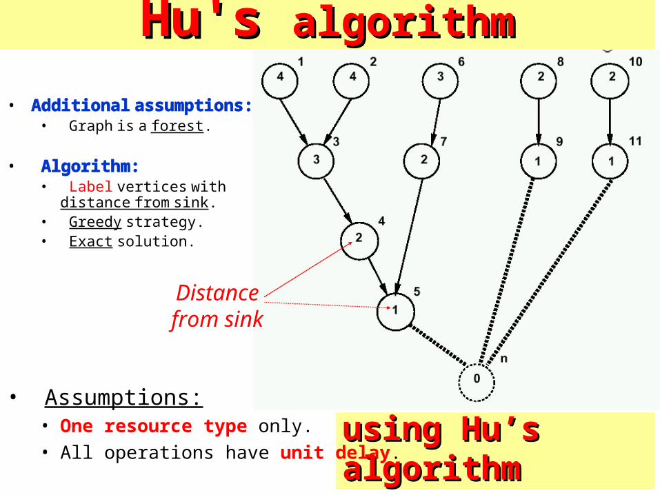
• Assumptions:• One resource type only.• All operations have unit delay.

Distance from sink

• Additional assumptions:• Graph is a forest.

• Algorithm:• Label vertices with distance

from sink.• Greedy strategy.• Exact solution.

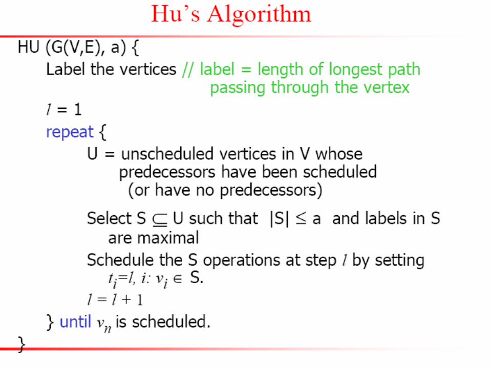
Hu's Hu's algorithmalgorithm

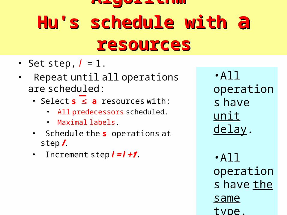
Algorithm Algorithm

Hu's schedule with Hu's schedule with aa resources resources• Set step, l = 1.• Repeat until all operations are

scheduled:• Select s a resources with:

• All predecessors scheduled.• Maximal labels.

• Schedule the s operations at step l.• Increment step l = l +1.

•All operations have unit delay.

•All operations have the same type.

• Minimum latency with a = 3 resources.• Step 1:

• Select {v 1 , v 2 , v 6 }.

• Step 2: • Select {v 3 , v 7 , v 8 }.

• Step 3: • Select {v 4 , v 9 , v 10 }.

• Step 4: • Select {v 5 , v 11 }.

Algorithm Algorithm

Hu's schedule with Hu's schedule with aa resources resources

We always select 3 resources

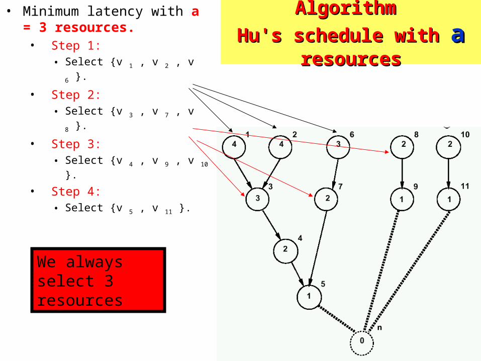
• Minimum latency with a = 3 resources.• Step 1:

• Select {v 1 , v 2 , v 6 }.

• Step 2: • Select {v 3 , v 7 , v 8 }.

• Step 3: • Select {v 4 , v 9 , v 10 }.

• Step 4: • Select {v 5 , v 11 }.

Algorithm Algorithm

Hu's schedule with Hu's schedule with aa resources resources

We always select 3 resources

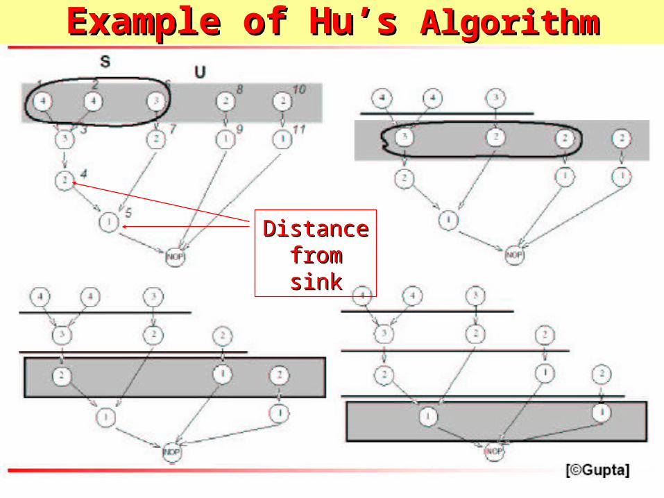
Example of Hu’s Example of Hu’s AlgorithmAlgorithm

Distance Distance from sinkfrom sink

Example Example of Hu’s of Hu’s

AlgorithmAlgorithm

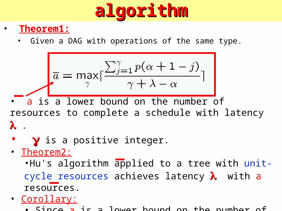
Exactness of Hu's algorithmExactness of Hu's algorithm• Theorem1:

• Given a DAG with operations of the same type.

• a is a lower bound on the number of resources to complete a schedule with latency .

• is a positive integer.• Theorem2:

•Hu's algorithm applied to a tree with unit-cycle resources achieves latency with a resources.

• Corollary:• Since a is a lower bound on the number of resources for achieving , then is minimum.

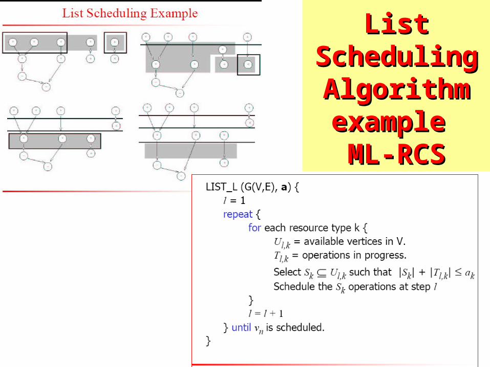
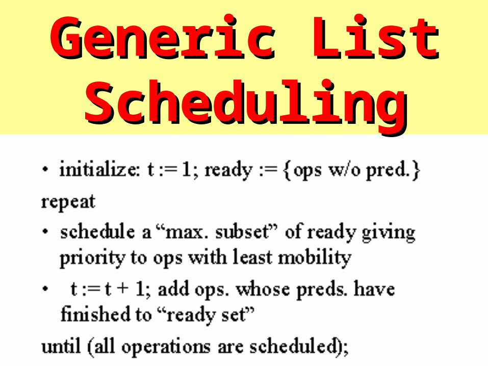
LIST LIST schedulingscheduling

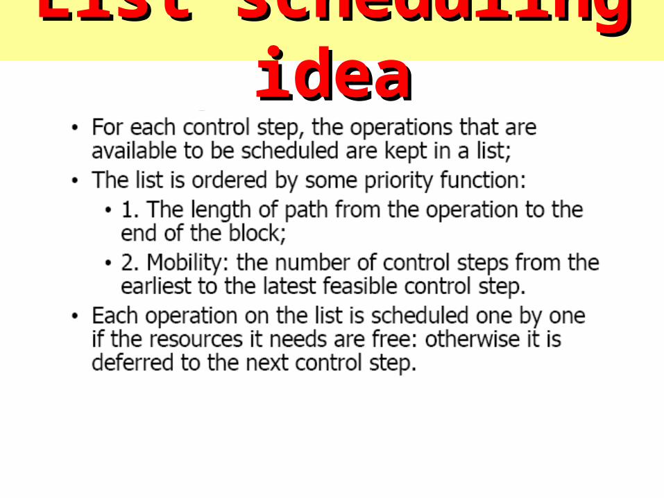
List scheduling ideaList scheduling idea

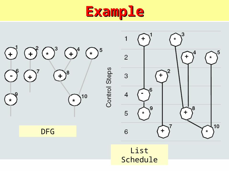
ExampleExample

DFG

List Schedule

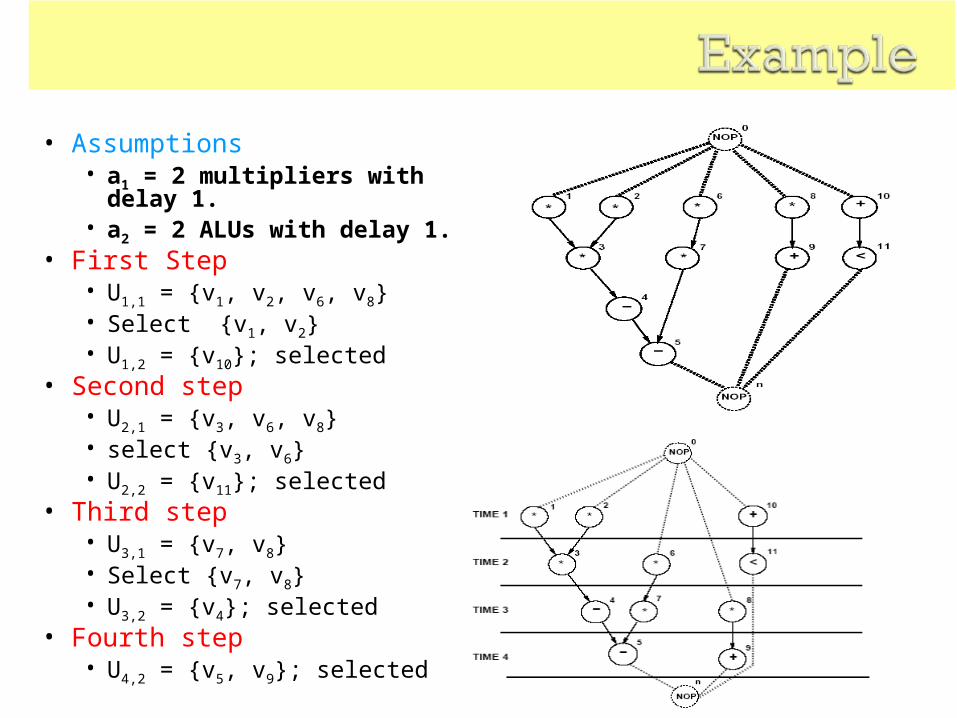
• Assumptions• a1 = 2 multipliers with delay

1.• a2 = 2 ALUs with delay 1.

• First Step• U1,1 = {v1, v2, v6, v8}• Select {v1, v2}• U1,2 = {v10}; selected

• Second step• U2,1 = {v3, v6, v8}• select {v3, v6}• U2,2 = {v11}; selected

• Third step• U3,1 = {v7, v8}• Select {v7, v8}• U3,2 = {v4}; selected

• Fourth step• U4,2 = {v5, v9}; selected

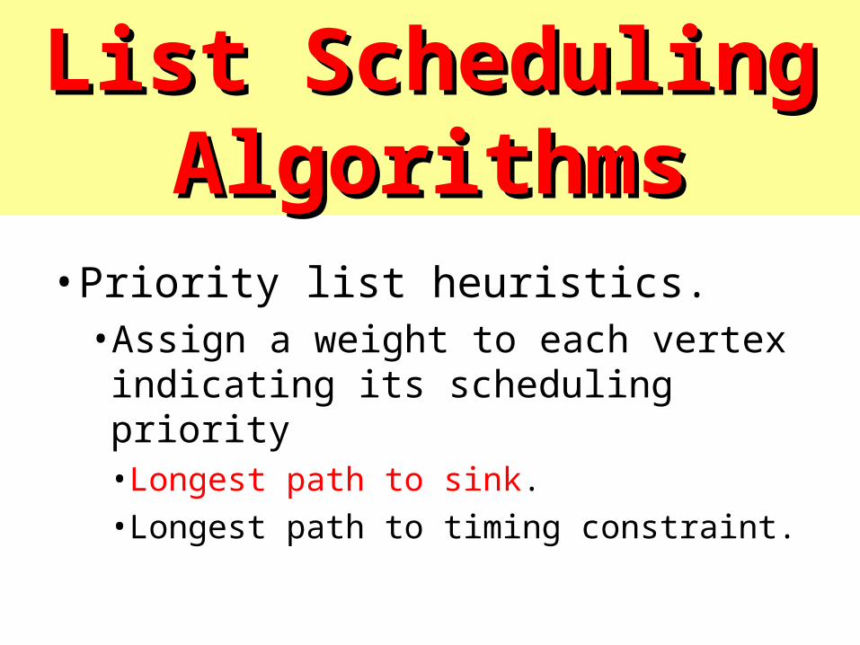
•Priority list heuristics.•Assign a weight to each vertex indicating its scheduling priority•Longest path to sink.•Longest path to timing constraint.

List Scheduling List Scheduling AlgorithmsAlgorithms

List schedulingList scheduling algorithmsalgorithms

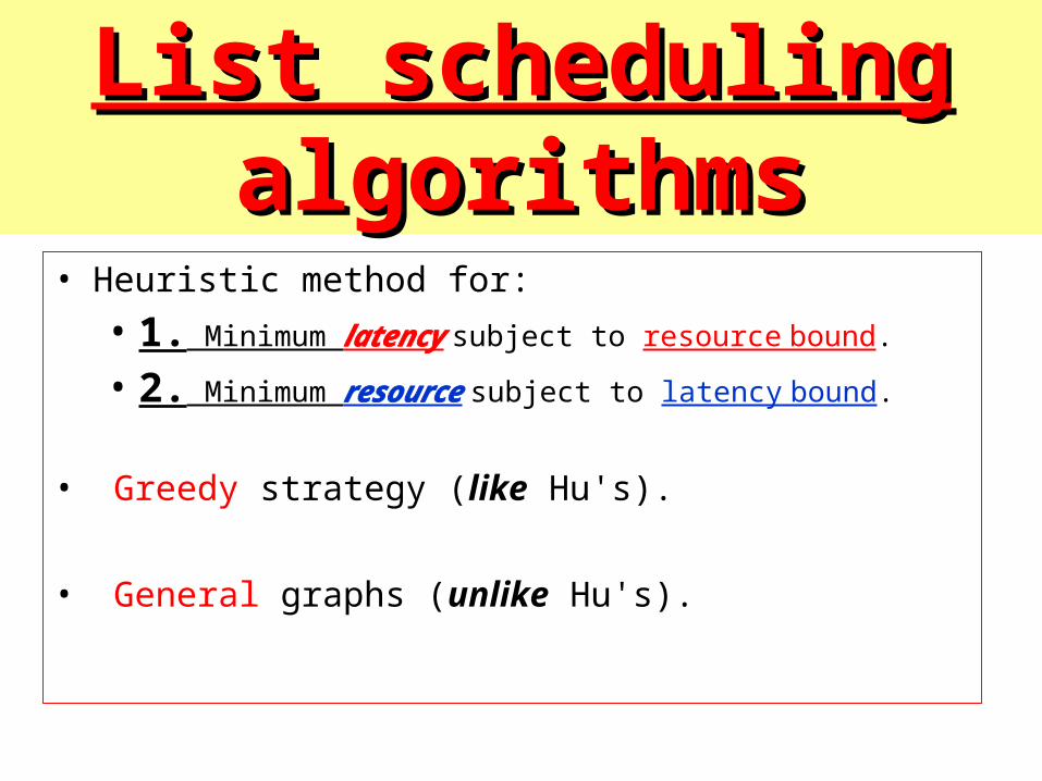
• Heuristic method for:

• 1. Minimum latency subject to resource bound.

• 2. Minimum resource subject to latency bound.

• Greedy strategy (like Hu's).

• General graphs (unlike Hu's).

LIST schedulingLIST scheduling

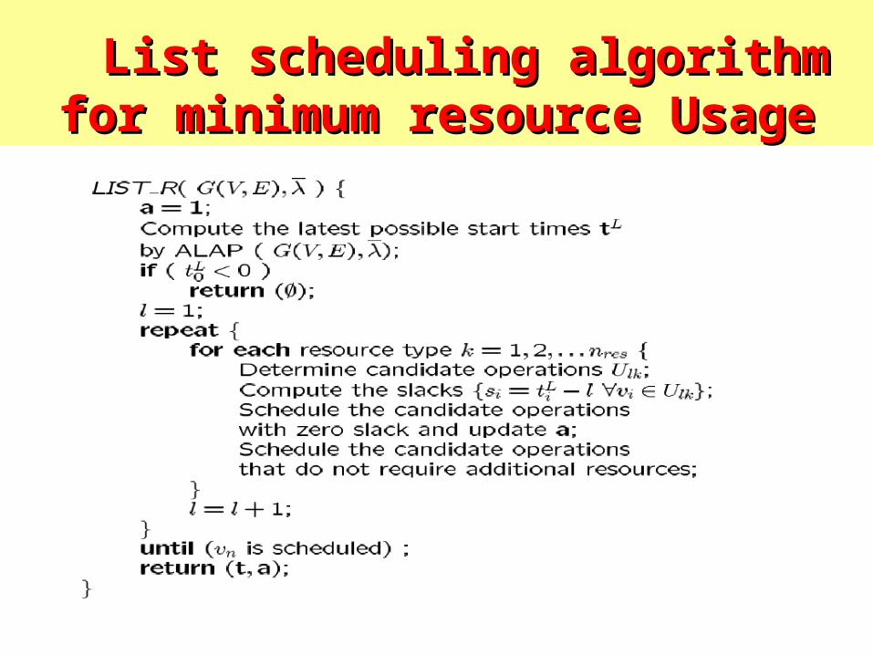
List scheduling algorithmList scheduling algorithmfor minimum resource Usagefor minimum resource Usage

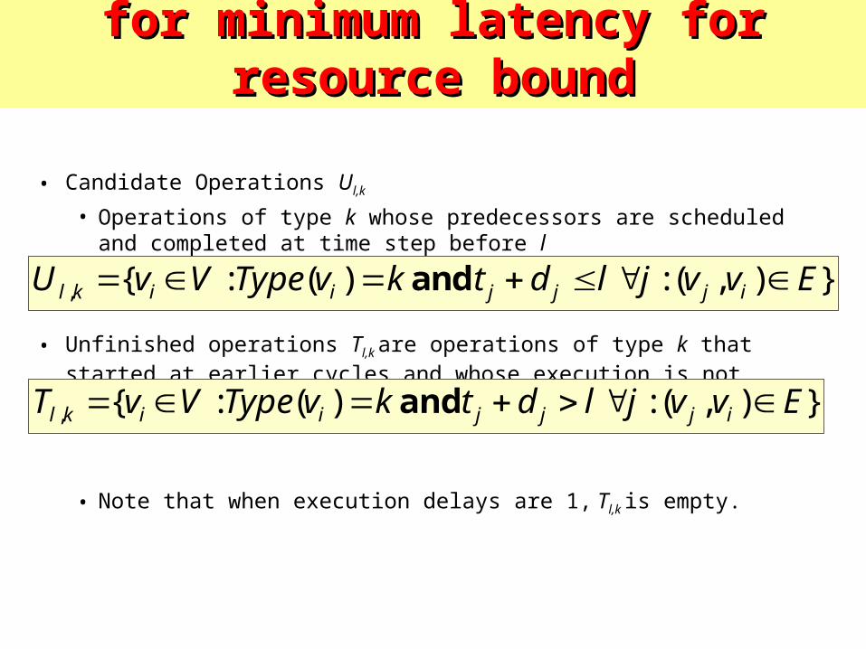
• Candidate Operations Ul,k

• Operations of type k whose predecessors are scheduled and completed at time step before l

• Unfinished operations Tl,k are operations of type k that started at earlier cycles and whose execution is not finished at time l

• Note that when execution delays are 1, Tl,k is empty.

}),(:)(:{, Evvjl dtkvΤypeVvU ijjjiikl and

}),(:)(:{, Evvjl dtkvΤypeVvT ijjjiikl and

List scheduling algorithmList scheduling algorithmfor minimum latency for resource boundfor minimum latency for resource bound

List scheduling algorithmList scheduling algorithmfor minimum latency for resource boundfor minimum latency for resource bound

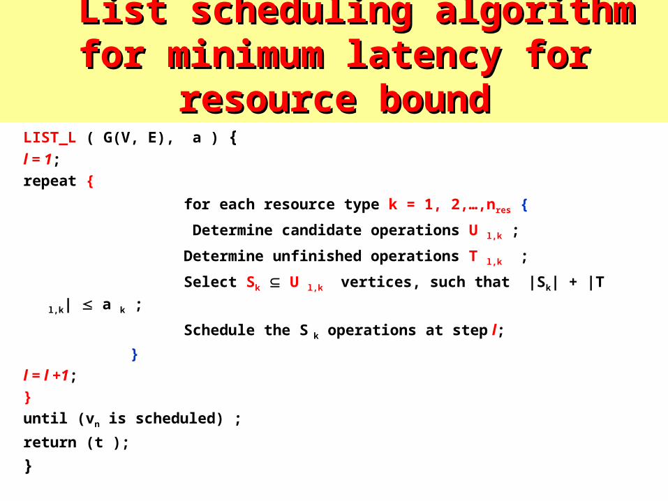
LIST_L ( G(V, E), a ) {l = 1;repeat {

for each resource type k = 1, 2,…,nres {

Determine candidate operations U l,k ;

Determine unfinished operations T l,k ;

Select Sk U l,k vertices, such that |Sk| + |T l,k| a k ;

Schedule the S k operations at step l;

}l = l +1;}until (vn is scheduled) ;

return (t );

}

• Assumptions:• a 1 = 3 multipliers with

delay 2.

• a 2 = 1 ALUs with delay 1.

List scheduling algorithmList scheduling algorithmfor minimum latencyfor minimum latency

1. List scheduling algorithm1. List scheduling algorithmfor minimum latency for resource boundfor minimum latency for resource bound

Now we needtwo time units for multiplier

• Assumptions• a1 = 3 multipliers with delay

2.

• a2 = 1 ALU with delay 1.

ExampleExample

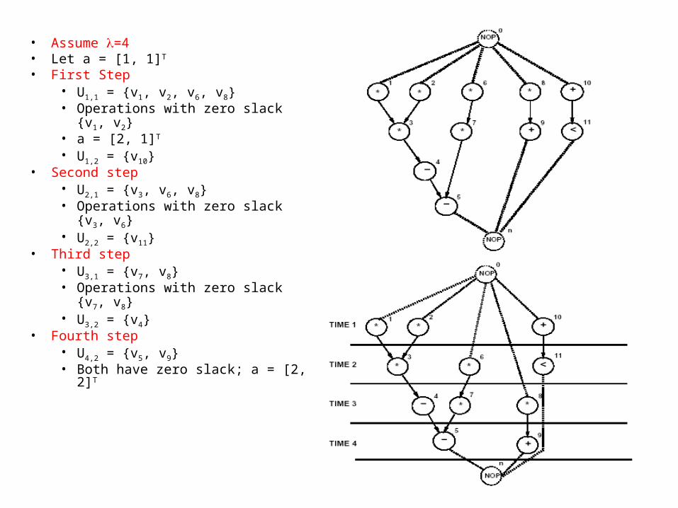
• Assume =4• Let a = [1, 1]T

• First Step• U1,1 = {v1, v2, v6, v8}• Operations with zero slack {v1, v2}• a = [2, 1]T

• U1,2 = {v10}• Second step

• U2,1 = {v3, v6, v8}• Operations with zero slack {v3, v6}• U2,2 = {v11}

• Third step• U3,1 = {v7, v8}• Operations with zero slack {v7, v8}• U3,2 = {v4}

• Fourth step• U4,2 = {v5, v9}• Both have zero slack; a = [2, 2]T

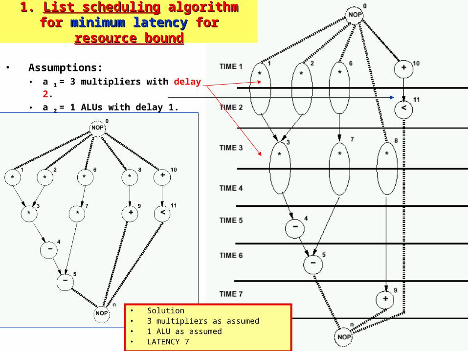
• Assumptions:• a 1 = 3 multipliers with delay 2.

• a 2 = 1 ALUs with delay 1.

1. 1. List schedulingList scheduling algorithm algorithmfor for minimum latencyminimum latency for for resource boundresource bound

• Solution• 3 multipliers as assumed• 1 ALU as assumed• LATENCY 7

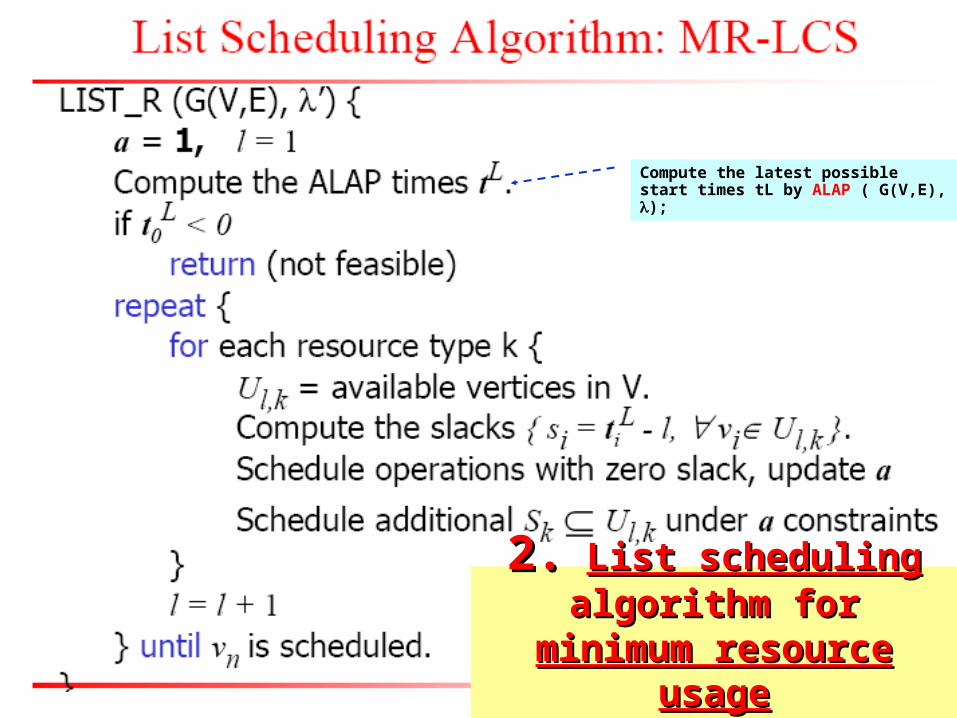
Compute the latest possible start times tL by ALAP ( G(V,E), );

2.2. List schedulingList scheduling algorithm algorithm for for minimum resource usageminimum resource usage

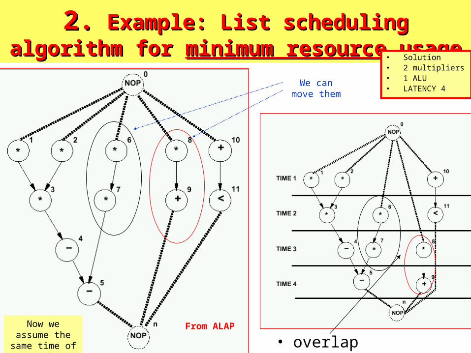
• overlap

2.2. Example: List scheduling algorithm for Example: List scheduling algorithm for minimum resource usageminimum resource usage

From ALAP

We can move them

• Solution• 2 multipliers • 1 ALU • LATENCY 4

Now we assume the same time of each operation

List Scheduling Algorithm example List Scheduling Algorithm example ML-RCSML-RCS

** * *

* *

-

-

+

+

<

Assume 3 multipliers Assume 1

ALU

t=0mul 3m 1 ALU

t=1 1 ALU

t=2 3mul

t=3 1 ALU

t=4 1 ALU

t=5 1 ALUNow we assume the same time of

each operation

Other way of explanation of the same as in last

slide

List List Scheduling Scheduling Algorithm Algorithm example example ML-RCSML-RCS

Generic List Generic List SchedulingScheduling

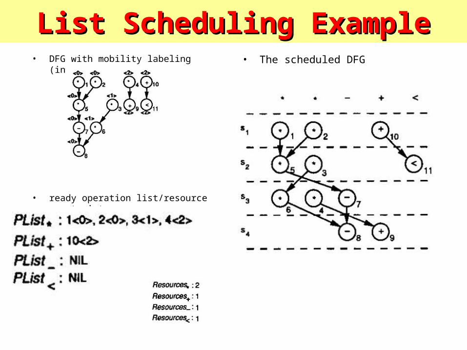
List Scheduling ExampleList Scheduling Example• The scheduled DFG• DFG with mobility labeling (inside <>)

• ready operation list/resource constraint

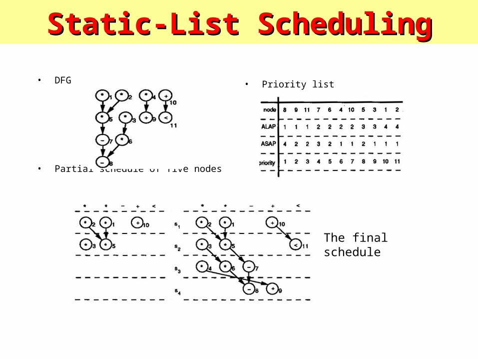
Static-List SchedulingStatic-List Scheduling

• DFG

• Partial schedule of five nodes

• Priority list

The final schedule

Classification of Classification of Scheduling ApproachesScheduling Approaches

Classification of Classification of Scheduling ApproachesScheduling Approaches

Classification of Scheduling Classification of Scheduling ApproachesApproaches

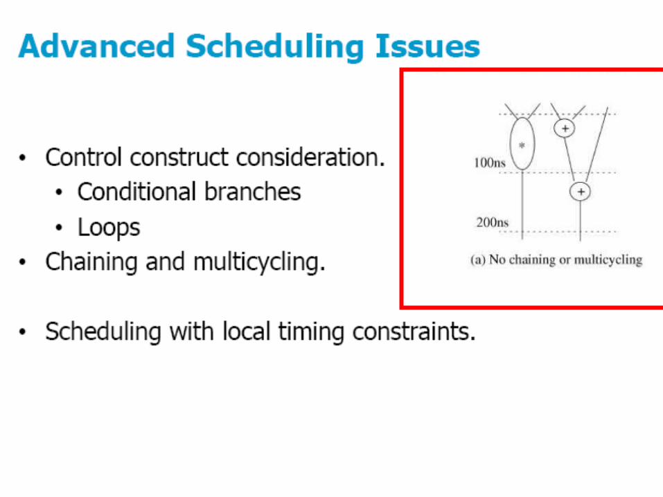
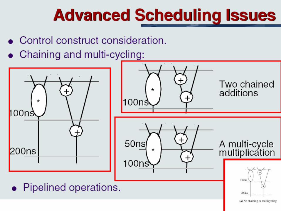
Scheduling with chainingScheduling with chaining• Consider propagation delays of resources not in terms of cycles.

• Use scheduling to chain multiple operations in the same control step.

• Useful technique to explore effect of cycle-time on area/latency trade-off.

• Algorithms:• ILP, • ALAP/ASAP, • List scheduling.

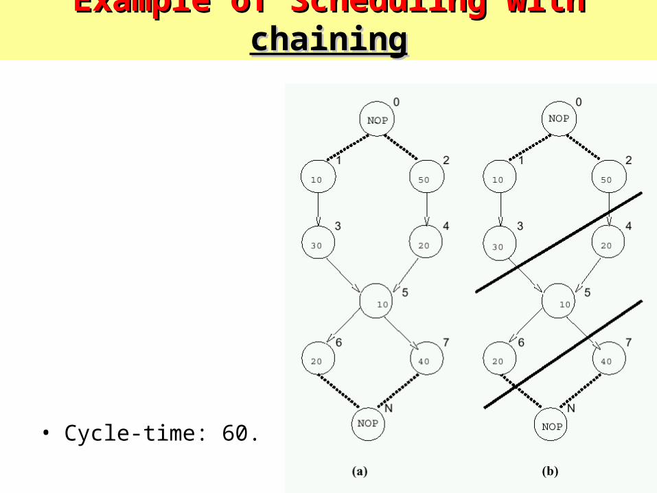
Example of Scheduling with Example of Scheduling with chainingchaining

• Cycle-time: 60.

SummarySummary

• Scheduling determines area/latency trade-off.• Intractable problem in general:

• Heuristic algorithms.• ILP formulation (small-case problems).

• Chaining:• Incorporate cycle-time considerations.

Other scheduling Other scheduling approachesapproaches

Three variants ofThree variants of SchedulingScheduling

Finite Impulse Finite Impulse Response FilterResponse Filter

D

* *

+

*

D

+

*

D

+

*

D

+

*

D

+

*

D

+

*

D

+

*

D

+

*

D

+

*

D

+

IN[i]

OUT

c0 c3c2c1 c7c6c5c4 c10c9c8

A0

A0

A3A2A1 A6A5A4 A8A7 A9

B0 B1

B1

B4B3B2 B5 B7B6 B8 B9

IN[i-1] IN[i-2] IN[i-6]IN[i-5]IN[i-4]IN[i-3] IN[i-8]IN[i-7] IN[i-10]IN[i-9]

This can be directly used for synthesis with 11 multipliers, 10 adders and 10 registers. But the latency would be 1 multiplier + 10 adders

Example 1

FIR FIR SchedulingScheduling+

+

+

+

+

+

+

*

*

*

*

*

*

*

*

*

*

+

+

+

*

1

10

9

8

7

6

5

4

3

2

11

c0 c1

c2

c3

c4

c5

c6

c7

c8

c9

c10

A0

A4

A3

A2

A1

A5

A6

A7

A8

A9

B0

B3

B2

B1

B4

B6

B5

B9

B8

B7

IN[i] IN[i-1]

IN[i-6]

IN[i-5]

IN[i-4]

IN[i-3]

IN[i-2]

IN[i-8]

IN[i-7]

IN[i-9]

IN[i-10]

OUT

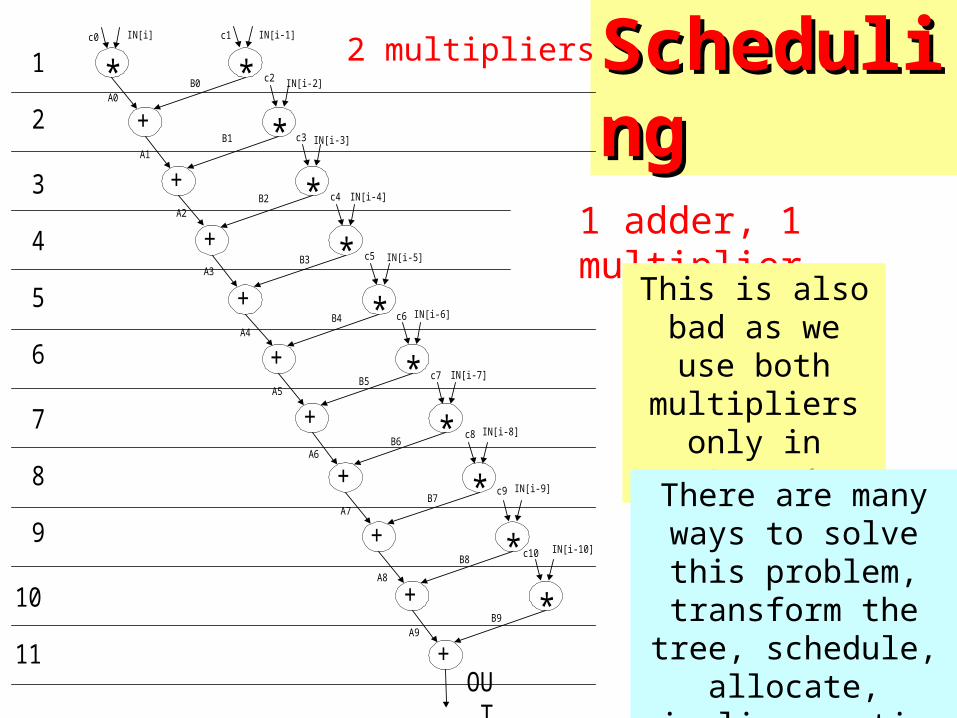
1 adder, 1 multiplier

2 multipliers

This is also bad as we use both

multipliers only in stage 1

There are many ways to solve this problem,

transform the tree, schedule, allocate,

pipeline, retime

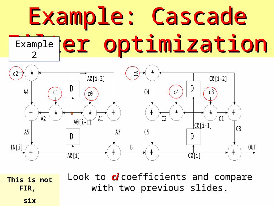
Example: Cascade Filter Example: Cascade Filter optimizationoptimization

IN[i] OUT+ +

+ +

*

**

D

D

+ +

+ +

*

**

D

D

A0[i]

A0[i-1]

A0[i-2]

A1A2

A5

A4

A3

c0c1

c2

BC0[i]

C0[i-1]

C0[i-2]c5

c4 c3

C1

C5

C4

C2

C3

Look to ci ci coefficients and compare with two previous slides.

Example 2

This is not FIR,

six coefficients

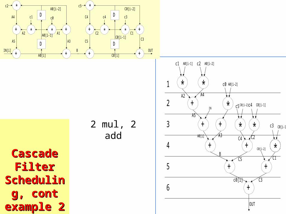
Cascade Cascade Filter Filter

Scheduling, Scheduling, cont example cont example

22

* *

+

*********

+

+

+

+

+ *

+

* *

+

1

2

3

4

5

6

OUT

c1

c4c5

c0

c2

c3

A0[i-1] A0[i-2]

A0[i-2]

C0[i-1]

C0[i-1]C0[i-2]

A2 A4

A5

A0[i] A3

BC5

c0[i] C3

C1

C2C4

C0[i-2]

IN

IN[i] OUT+ +

+ +

*

**

D

D

+ +

+ +

*

**

D

D

A0[i]

A0[i-1]

A0[i-2]

A1A2

A5

A4

A3

c0c1

c2

BC0[i]

C0[i-1]

C0[i-2]c5

c4 c3

C1

C5

C4

C2

C3

2 mul, 2 add

Infinite Impulse Infinite Impulse Response FilterResponse Filter

**

IN+ +

D

D

+ +**

OUT

**

+ +

D

D

+ +**

D

+

*

+

*

A0[i]

A0[i-1]

A0[i-2]

C0[i] D0[i]

D0[i-1]

C0[i-1]

c0 c8c9

c6c7

c4c5

c3 c2

c1 A1

A4 A3

A2 C1

C3

B

C0[i-2]

C4

C2

D

D1D2

C5C6A5A6

Example 3

IIR Filter, 10 coefficients

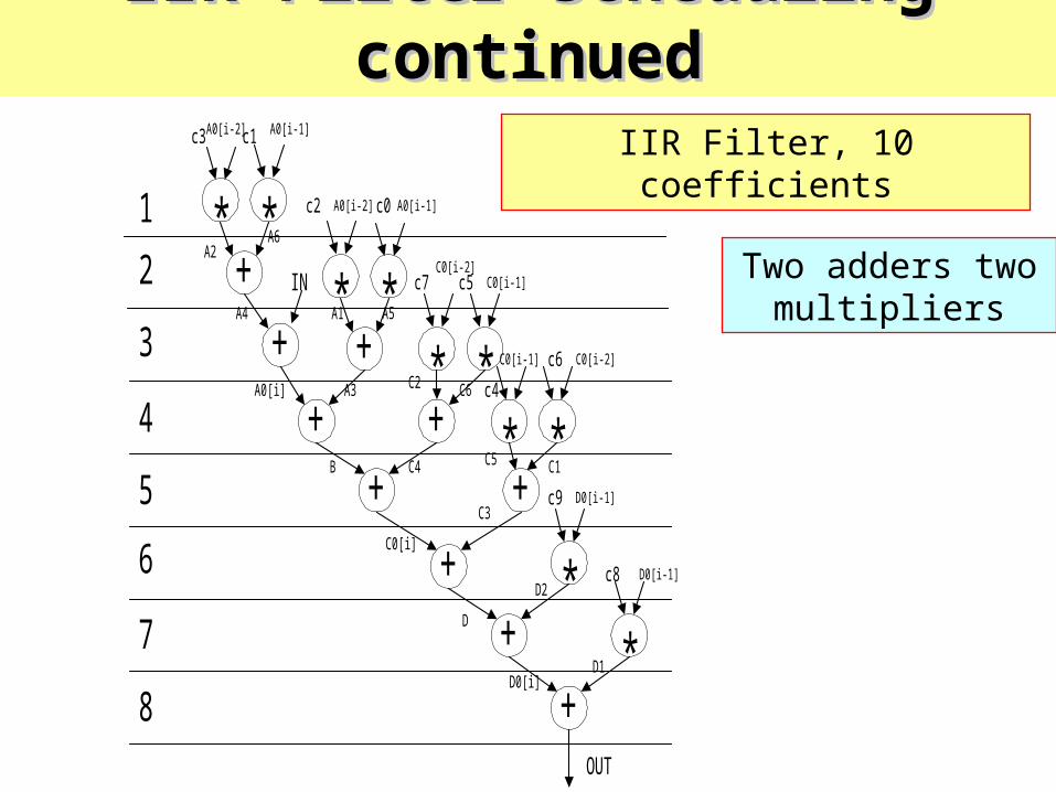
IIR Filter Scheduling continuedIIR Filter Scheduling continued

*+

*

+

+

+

+

++ +

++

*

*** *

*

**

1

7

3

4

6

5

2

8

c3

c4

c6

c5c7

c0c2

c1

c8

c9

A0[i-2] A0[i-1]

A0[i-2] A0[i-1]

C0[i-2]C0[i-1]

C0[i-1] C0[i-2]

D0[i-1]

D0[i-1]

A2

D1

D2

C3

D0[i]

D

C0[i]

B

A3A0[i]

A4

A6

C6C2

A5A1

C1C5C4

OUT

IN

IIR Filter, 10 coefficients

Two adders two multipliers

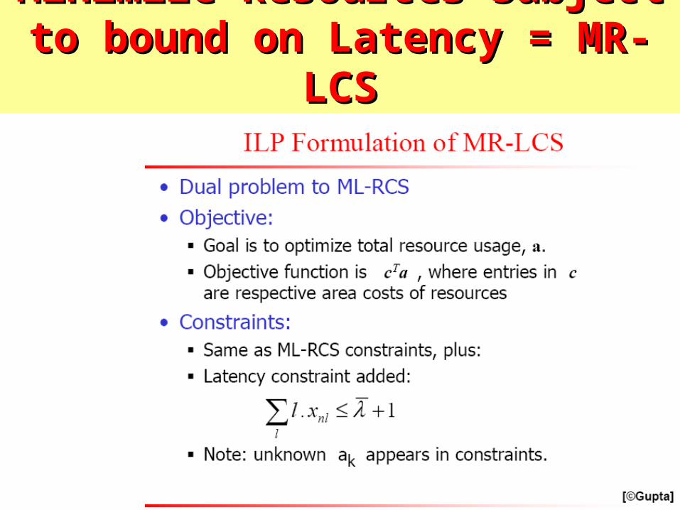
Minimize Resources Subject to Minimize Resources Subject to bound on Latency = MR-LCSbound on Latency = MR-LCS