Scheduling Page 2 · The scheduling problem (Chapter 9) ... Short-term scheduling Monday, November 22, 2004 ... Scheduling Page 15 . Exponential distribution:

The scheduling problem (Chapter 9)○ Decide which processes are allowed to run when. ○ Optimize throughput, response time, etc. ○ Subject to constraints including context switch

time, swap time, etc.

Kinds of scheduling: ○ Short term: which process, already in memory,

gets a slice of time next. ○ Medium-term: which processes are loaded

partially or fully into memory. ○ Long term: which processes are "admitted" for

later processing. AKA "admission control". ○ I/O: which pending I/O request should be

handled first?

Scheduling Monday, November 22, 200410:22 AM

Scheduling Page 1

Scheduling Page 2

Long-term scheduling○ Also known as "admission control". ○ A big research topic in grid computing

right now.

Questions asked by a long-term scheduler: ○ How many concurrent processes can the

system handle? ○ How much memory is needed for each? ○ How important is response time versus

throughput versus efficiency?

Scheduling Page 3

Long-term scheduling factors○ Response time: how long until one gets

an answer to a problem? ○ Example: weather forecasting must be

finished before the 7pm news. ○ Throughput: how much of the cpu can

one use by latency hiding?○ Example: How fast can one finish n

predictions of geological substructure, ○ where n is large?

Scheduling Page 4

Typical admission control algorithm○ Predict resource utilization.○ Predict overlap and latency hiding. ○ Admit process only if within bounds. ○ Otherwise, defer process until there are

enough resources to assure completion. ○ (banker's algorithm)

Application: grid computing○ Process: a parallel program that runs on

a grid. ○ Resource utilization: # of nodes required,

amount of memory on each node (I/O bandwidth to each node)

○ Resources must be known in advance○ (not a problem for grid applications)

Scheduling Page 5

Medium-term schedulingEssentially, the swapping algorithmMost common strategy: least recently used (LRU).

Keep track of time since each page was accessed by a process last. Always swap out page that was least recently accessed.

Less common strategies: lookahead.Try to predict cpu access pattern. Preload pages that might be accessed next.

Medium term scheduling Monday, November 22, 200411:56 AM

Scheduling Page 6

Short-term schedulingDeals with processes that are not blocked waiting for swap-out, swap-in. Behavioral aspects:

Throughput: how much work is performed. Response time: how quickly are units of work completed, once requested.

All scheduling algorithms choose a balance between these criteria.

Short-term scheduling Monday, November 22, 200411:59 AM

Scheduling Page 7

Priorities○ Priority: a number than indicates how

important a process is, in terms of response time.

○ Low priority: response time unimportant. ○ High priority: response time very

important. ○ Key to our discussion: running high

priority processes is not enough; low-priority processes still need to satisfy response-time limits.

Note: the game here is to balance: round-robin scheduling (equal slices)

optimal for response time over homogeneous client base.

run to block: keep going until you can't.optimal for batch: no context switches.

Scheduling Page 8

Decision modes: ○ Non preemptive: once process runs, it stays running

till blocked or exit. ○ Preemptive: once a process is scheduled, it is still

pre-empted later in order to allow others to run.

Scheduling algorithmsFirst-come, first-serve (FCFS): queue unblocked processes, run each until blocked.

non-preemptiveminimum overhead.

Round-robin: execute each process for a little of the time available, grant slice times relative to priority.

PreemptiveFair treatment

Shortest Process Next (SPN): priority queued, allow the process with the shortest "expected" time to run next.

Non-preemptive. Must predict runtimeWorks best with lots of little processes or phases: average runtime is good predictor. used in RTOS's

Shortest Remaining Time (SRT): priority queued, the process with the shortest predicted remaining time goes first.

Non-preemptiveMust predict runtime.

Highest Response Ratio Next (HRRN): choose process with highest response ratio.

Non-preemptive.Response ratio = (w+s)/s

w=time spent waiting for processors=expected computation time

Feedback: establish several queues, each with lower priority than preceeding; bubble down processes in the queues.

Preemptive. Queue position = priority.

Scheduling Page 9

Queue position = priority.Priority changes with time spent computing.

Scheduling Page 10

Scheduling Page 11

Problem: which one of these works best in my environment.

Solution: can analyze the response of systems with queueing theory.

HistoryEarly machines were batch processors. Job time was often predictable:

Accounts payable: time≈# checks to write!Compilation: time≈program lengthEtc.

Question: how to predict throughput based upon what we know about a system. Answer: queueing theory and simulation

Queueing theoryMathematical model of batch processing. Overly precise models that almost model reality. Precise answers to a number of specific questions. No information in many realistic cases.

SimulationMessy replication of processing operations. Results as accurate as the detail with which it is simulated.Sensitive to sloppiness in coding simulator behaviors.

Queueing theory assumptions: Poisson arrival of jobs. Exponential service times. Whoa there! What is going on here?

Queueing theory Monday, November 22, 200412:16 PM

Scheduling Page 12

Poisson process: ○ Models arrival time as a set of completely

independent trials.○ Let t be the time of arrival of the next

event, as a difference between now and then. Then:

Prob(arrival time t≤q) = 1-e-λq

λ: the rate of the process; a measure of how fast things happen.

Small λ: events are spaced far apart. Large λ: events are spaced close together.

Poisson processes Monday, November 22, 200412:30 PM

Scheduling Page 13

Scheduling Page 14

Facts about Poisson distributions○ Mean = 1/λ○ Standard deviation = 1/λ○ Memoryless: Prob(T≤x+t|T>t)=Prob(T≤x)○ In other words, waiting longer (T>t) doesn't

change things. ○ Suppose X,Y,Z are independent Poission

processes with parameters λX,λY,λZ. Then the union of X,Y,Z is Poisson with parameter λX+λY+λZ

○ In other words, the union of a set of Poisson arrivals is Poisson, with the obvious parameter.

Scheduling Page 15

Exponential distribution:Prob(Processing time ≤ t) = 1-e-μt

μ = parameter of jobs. Mean = 1/μStandard deviation = 1/μMemoryless: Prob(T≤x+t|T>t)=Prob(T≤x)

Exponential distribution Monday, November 22, 20041:13 PM

Scheduling Page 16

Same equation, different meanings: ○ A Poisson process is one in which the

inter-event arrival times are exponential.

○ An exponential variable is one in which the value of the variable follows an exponential distribution.

○ Same equation, two meanings. Prob(next event before time t) = 1-e-λt

Prob(processing time less than t) = 1-e-μt

○ This symmetry makes analysis a lot easier than if these were different!

What's going on? Monday, November 22, 20041:27 PM

Scheduling Page 17

Scheduling Page 18

Poisson postulatesa. Prob(1 arrival in Δt) = λΔtb. Prob(>1 arrival in Δt) = o(Δt) and

negligible.c. Arrival time is independent of other arrivals

and last arrival.

Scheduling Page 19

Combination/multiplexing:

Splitting/demultiplexing:

π1+π2+…+πn=1.00≤πi≤1.0πi is a constant probability of taking branch i.

Simple Poisson Properties Monday, November 22, 20047:29 PM

Scheduling Page 20

Simple queueing Monday, November 22, 20047:36 PM

Scheduling Page 21

Kinds of queues○ Kendall notation: A/B/c/k/m/Z○ A=arrival process; default is M (Poisson) ○ B=service process; default is M (Exponential) ○ c=number of servers; default is 1○ k=maximum queue size; default is infinite○ m=customer population; default is infinite○ Z=name of queueing discipline, default is FCFS

Previous queue is M/M/1Here's M/M/3:

Scheduling Page 22

Some startling mathematical results:

For M/M/1 queue, Queue reaches steady state only if λ/μ<1Prob(queue length is n) = pn(1-p) where p=λ/μThe mean queue length (enqueued jobs) is n=p/(1-p). The mean waiting-line length (jobs not being served) is w=p2/(1-p) (this includes jobs in process of being queued and dequeued)

Little's laws: for M/M/1 queue: Mean time in system = n/λMean wait time before service = w/λ

Key to proofs: principle of balance: input rate = output rate if system is in balance (lambda<mu)

Scheduling Page 23

Generalization: c processors:Steady state: λ/cμ<1 S0=Prob(queue empty)=

Mean time prior to service=

The M/M/c queue Monday, November 22, 20048:09 PM

Scheduling Page 24

Infinite consumers, Poisson arrival(monkeys on keyboards)

Waiting line length = w = 0Mean time in system = 1/μMean queue length = λ/μ

The M/M/∞ Queue Monday, November 22, 20048:14 PM

Scheduling Page 25

Networks of queues○ Can connect queueing systems together

into networks○ Output of one system is input to another. ○ Surprising result: can compute the

parameters of the network provided one knows the distribution parameters of inputs and service parameters of the queues.

Key concept: "stability" is simpler to analyze than dynamic state. ○ To achieve stability, system must come

into "equilibrium" subject to "balance equations".

○ Key equilibrium: input=output. ○ In absence of this balance, system cannot

be analyzed easily. ○ When equilibrium is present, analysis is

easy!

Networks of Queues Monday, November 22, 20048:18 PM

Scheduling Page 26

First case: no feedback

Scheduling Page 27

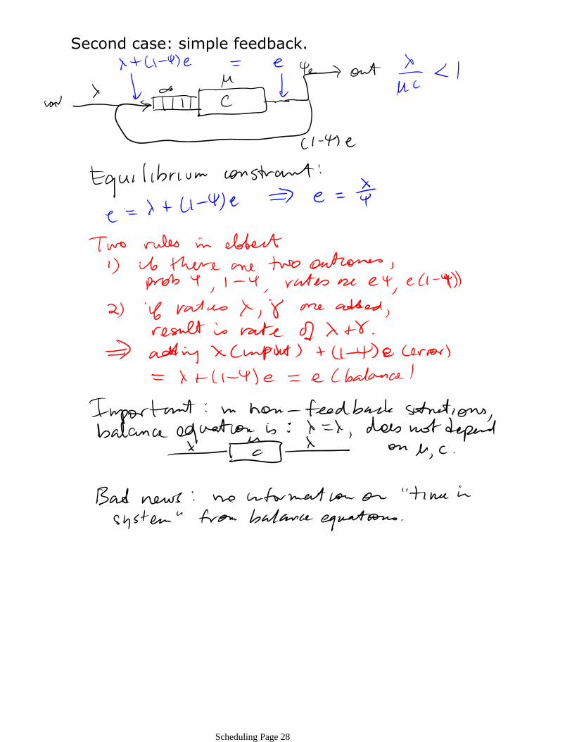
Second case: simple feedback.

Scheduling Page 28

Case 2: feedback in open networks (input from outside, output to outside)

Queues 1-q with server constants µi, ci servers.Each queue gets input from all other queues, and input from outside world. Prob(queue i gets input from queue j) = πji

Prob(queue i output exits network) is ψi

Each queue's view of the world:

Note: ○ λk, ψk, πjk μk, ck constant. ○ Variables are e1, …, eq

○ q equations in q unknowns → unique solution. ○ If this solution exists, it is the equilibrium point!

("Jackson's algorithm")

Scheduling Page 29

Alas, some systems are "closed": ○ Example: fixed number of users typing on

keyboards and receiving responses. ○ Every input gets a response. ○ Every response generates an input. ○ Can model this as a "closed" system.

Closed-world situation○ Fixed number of jobs N circulate within the

system. ○ No input from outside the system. ○ At any time, the sum of jobs in all queues is

N: If ni is the number of jobs in the queue for server i, then ∑i ni = N

Unfortunately, the simple Jackson method doesn't work in closed systems in which requests circulate and no request is ever deleted.

Linear system is underdetermined. Too many solutions!

Problem description:N requests. K server queues. A state of the system is a vector (n1, …, nK) describing how many requests are queued for each server. Let vi represent the input rate for queue i. Let pkm represent the probability that the output of queue k will be assigned to the input of queue m. Jackson's equations:

Closed systems Tuesday, November 30, 20041:29 PM

Scheduling Page 30

Jackson's equations: vm = ∑pkmvk

are underdetermined.

Eureka!All we're interested in is a steady state of the system. If such a state exists, it has some extremely simple properties. In particular,

output=input (Jackson's equations) But, more specifically,

The probability of a specific steady state must be independent of any prior state.

Method: normalization constants: Compute probability of each state in a steady-state solution= Prob(n1,…,nK) = (probability that queue 1 has n1 elements and queue 2 has n2 elements … and queue K has nK elements) A really dirty trick: we know it's independent, so that it's proportional to ∏ (probability that queue i has ni

elements) (product of all of these) = ∏ pi

ni (pi

ni is probability that queue i has

ni elements)= ∏ (vi/µi)ni (by previous discussion of M/M/1 queues)

Key: ○ Assume the existence of a proportionality

constant G(N) so that Prob (state n1,…,nK) = 1/G(N) ∏ (vi/µi)n

i

Scheduling Page 31

1/G(N) ∏ (vi/µi)ni

So that∑ Prob(state n1,…,nK) = 1.0

○ If we can compute G(N), we know the probabilities for states, which in turn means that we know the expected aggregate state

E=∑ (n1,…,nK) Prob(n1,…,nK)Which predicts how long each queue is during steady-state behavior.

○ With this, we have all we need to compute any throughput parameter.

Big problem: combinatorial explosionTo compute G(N), must sum over all states. There are lots of states!How to cope?

Solution: Buzen's algorithmBuild network incrementallyBase new normalization constant on constants for smaller networks.

Implementing Buzen's algorithmgK(N) = normalization constant for K servers, N jobs. gn(0) = 1 for all ng1(n)= probability that queue 1 has length n = (v1/µ1)n

gm(n)=gm-1(n)+(vm/µm)gm(n-1)In short, build the network one server at a time, compensate for that server's behavior.

Not all is won: Note: at end of Buzen's algorithm, we have GK(N) in terms of vi

But we still don't know vi

Must still apply Jackson's system, using the

Scheduling Page 32

extra equation from here.

Scheduling Page 33

A whole course is possible(used to be on the qualifier for a Ph.D. in computer science) (fortunately, no longer!)

What we understandQueueing of load-independent servers

(tasks in queue don't affect response time)

Queueing of load-dependent servers(tasks in queue affect response time)

Distribution-independent results for very simple networks.

What we don't understandModels other than FCFS. Non-linear response. Non-equilibrium behavior.Etc.

Beyond simple queueing theory Tuesday, November 30, 20042:24 PM

Scheduling Page 34

Good news: queueing theory explains a lot of simple cases and illustrates basic properties○ Distribution parameter○ Processing parameter○ Queue length○ Time in system○ Etc.

Applicable to: ○ Typing at keyboard○ I/o requests coming from programs. ○ Service requests coming from network. ○ Disk performance.

Bad news: not realistic for many real systems○ λ is a variable over time. ○ All that is known only works for special cases.○ Accuracy of conclusions very sensitive to

assumptions made. ○ No closed-form solution to the general problem.

Not applicable to: ○ Situations in which parameters change over time. ○ Bursty behavior, e.g., hacking or denial of service.

Situations in which division of labor changes (πjk not constant)

To study unconstrained systems, must use simulation.

Why queueing theory fails Tuesday, November 23, 20042:19 PM

Scheduling Page 35

Given: Poisson constant λAnd: uniformly distributed random number generator. Compute: time between adjacent arrivals.

Basics: Probability density function (PDF): integral over interval is probability:

Cumulative distribution function (CDF)integral from minimum boundary to some number a:

Simulating Poisson Processes Tuesday, November 23, 200411:21 AM

Scheduling Page 36

Uniform Distribution:

Scheduling Page 37

Poisson Distribution: for one arrival time:

Scheduling Page 38

Idea: generate uniformly distributed random numbers, "twist" them into following a different distribution.

Start with CDFGenerate uniform random numbers on the Y axis.Project each value onto the X axis. Result: X axis values follow the CDF.

Scheduling Page 39

Reason this works:

Scheduling Page 40

Implementing Poisson simulation

So -(ln(1-drand48())/lambda has a Poisson distribution (because drand48() has a uniform distribution over [0,1))

Scheduling Page 41

Inside a simulator○ Some concept of timebase, e.g., a global clock. ○ A state variable for each server showing what

state it is in. ○ State transition logic for servers at job

initiation/completion. ○ Queue data structures for each required queue.

Simulator structures: Initialize all data structuresMain loop:

Compute server input events. Compute state transitions on servers. Record server output events. Increment time

End main loop.Report performance.

Computing server input eventsCompute delay timeWhile delay is active, do nothing except delay--. When delay==0, inject event and compute new delay.

Computing state transitionsWhen starting a server on a job

record starting time.Compute job length from distribution

When computing a job on a server, Advance time while doing nothing, until job length has passed.When past, load next job from queue into server.

Inside a simulator Tuesday, November 23, 20042:29 PM

Scheduling Page 42

p j qserver.

Scheduling Page 43

Pareto: describes distribution of sizes of disk files on disk, or in a user home directory.

PDF(x) = aba/xa+1

CDF(x) = 1-(b/x)a

a: rate factor; determines ratio of small-to-large b: starting (smallest) size (≠0)

Pareto distribution attributesNot memoryless; what files you have does determine what files you create!Starts at non-zero boundaryPolynomial increase over time, not exponential.

Pareto distribution is a reasonably good model for: Sizes of files on disk.User disk usage (sample=user) CPU utilization of a user over some time period.

Other important distributions Tuesday, November 23, 20042:38 PM

Scheduling Page 44