SCE’s Home Energy Report Program Savings Assessment Ex-Post Evaluation Results, Program Year 2014 Final Report October 30, 2015 revised CALMAC Study ID SCE0391.01 Prepared for Project Manager Southern California Edison 1515 Walnut Grove Avenue Rosemead, CA 91770 Miriam Fischlein DSM Program Measurement and Evaluation Prepared by Project Manager Applied Energy Group 500 Ygnacio Valley Road Suite 250 Walnut Creek, CA 94596 www.AppliedEnergyGroup.com Patrice Ignelzi Principal Associate Program Evaluation and Load Analysis Applied Energy Group Tel. 510.982.3533 [email protected]

Welcome message from author
This document is posted to help you gain knowledge. Please leave a comment to let me know what you think about it! Share it to your friends and learn new things together.
Transcript
SCE’s Home Energy Report Program Savings Assessment
Ex-Post Evaluation Results, Program Year 2014
Final Report
October 30, 2015 revised
CALMAC Study ID SCE0391.01
Prepared for
Project Manager
Southern California Edison 1515 Walnut Grove Avenue Rosemead, CA 91770
Miriam Fischlein DSM Program Measurement and Evaluation
Prepared by
Project Manager
Applied Energy Group 500 Ygnacio Valley Road Suite 250 Walnut Creek, CA 94596 www.AppliedEnergyGroup.com
Patrice Ignelzi Principal Associate Program Evaluation and Load Analysis Applied Energy Group Tel. 510.982.3533 [email protected]

Principal Investigators Craig Williamson Anthony Duer Tommy Williams Patrice Ignelzi
Applied Energy Group iii
Executive Summary
Background This report documents Applied Energy Group’s evaluation of savings from the Home Energy Report (HER) program that Opower operated for Southern California Edison (SCE) in 2014. Along with the savings results, this report describes the processes we used to validate the sample selection, estimate the savings, and remove savings by HER participants that were counted as part of other programs that SCE offered during the same period. As this is the second wave of the HER program, we refer to this program as Opower-2 in this report.
The Opower-2 program targeted residential accounts in the San Gabriel/Rancho Cucamonga portion of SCE‘s service territory. The Home Energy Reports, which compare program participants’ household energy use to that of similar neighbors, were sent out to customers beginning in March 2014 through December 2014. The program operated under a strict randomized control trial experimental design that was reviewed by the CPUC Energy Division. The sample of customers included 150,000 accounts, randomly assigned to one of two equal-sized groups: a treatment group (received HER reports) and control group (did not receive HER reports). There was a group of customers that had an issue with mismatched addresses in the billing system, which resulted in 3,813 of the 75,000 treatment group customers not receiving their HERs. In order to retain the integrity of the experimental design, per the preference of the CPUC Energy Division (CPUC ED), the mismatched customers were left in the all parts of the analysis, with exception of the upstream savings calculations.
The goal of this savings assessment was to provide ex-post estimates of savings for the period March 18, 2014 to December 31, 2014 that are attributable to the 2014 HER program, including:
kWh savings achieved by the program participants, minus their savings claimed by other SCE programs operating during that time;
peak kW savings calculated two ways, applying a load factor to the kWh savings based on using SCE’s load research data and direct estimation from hourly interval data, minus their kW savings claimed by other SCE programs operating during that time.
Analysis Methods We estimated per-participant energy impacts for the HER program using two methods: difference in differences and regression modeling. These analyses were based on monthly billing data, which allowed us to include the control group of non-participants to capture time-related variation in energy use among the program participants not due to the HER reports. The difference in differences method provided a preliminary estimate of monthly and annual energy savings that we were able to use as an initial estimate of savings. In order to estimate the savings more precisely, we also analyzed the data using a fixed-effects regression approach. This allowed us to refine the savings estimate to assess the possible influence of variables related to participation and weather and to reduce the uncertainty of the savings estimates by accounting for more of the difference between customers.
SCE Home Energy Reports Program – Savings Assessment
iv Applied Energy Group
To develop the program-level savings, we applied the monthly estimates from the regression model to the active customer accounts (to account for attrition due to customer move-outs). We then subtracted the incremental portion of savings being claimed for these participants due to their participation in SCE’s other downstream (i.e., rebate) programs and upstream (price markdown) lighting program during the HER treatment period.
We also conducted two analyses to assess the peak kW impacts of the Opower-2 program. We made one estimate by applying an average residential class load factor to the estimated kWh savings. We also developed an estimate using interval data for the treatment and control accounts, analogous to the way we estimated the preliminary energy savings. For both estimates we used the 3-day heat wave, September 15-17, 2014, using the DEER definition. The final peak kW results are from the interval data analysis. We contrast these approaches to determine if it is feasible to obtain reliable results through the lower cost, load factor approach.
Results The results are the ex-post savings estimates for the HER 2014 program year. The difference in differences method provided a preliminary energy savings estimate of 52.41 kWh for the year, per participant, amounting to 0.8% of their baseline usage from April through December. The regression modeling confirmed this annual savings level and provided more nuance to the estimates; the regression-based estimates were used to develop the final savings for the program.
Table ES-1 summarizes the monthly and annual energy savings for the HER program treatment period, April 2014 through December 2014. It shows per-participant annual savings of 51.52 kWh or 0.8%, with monthly savings ranging from a low of 0.4% in April 2014 rising to a maximum of 1.0% in the latter part of the year. The table shows the estimated treatment customer average energy savings, percent energy savings, number of participants included in the analysis month, and total estimated savings for the population of participants. The savings are statistically significant for each of the months included in the model and reported here. March was not statistically significant in either the difference in differences or the regression model, and so was excluded from the analysis for the final estimates.
Figure ES-1 shows these energy savings estimates graphically.

SCE Home Energy Reports Program – Savings Assessment
Applied Energy Group v
Table ES-1. Estimated HER 2014 Energy Savings
Month Participants
Average Per-Participant Savings (kWh) a % Savings
Total Savings, All Participants
(kWh) a April 73,472 1.87 0.36% 137,669
May 73,169 4.62 0.75% 337,921
June 72,847 6.17 0.93% 449,671
July 72,427 7.97 0.95% 577,270
August 72,087 8.50 0.96% 613,050
September 71,784 5.82 0.65% 418,133
October 71,415 6.37 1.01% 454,694
November 71,138 4.78 0.94% 339,842
December 70,833 5.41 0.97% 383,199
Total a 51.52 0.84% 3,711,449 a Total savings differences due to rounding of average per-participant displayed values
Figure ES-1. Average Per-Participant Energy Savings Estimates and 90% Confidence Intervals
The peak kW savings results using hourly interval data yielded statistically significant per-participant savings of 0.0120 kW, a peak demand reduction of 0.43%. The 90% confidence interval is +/- 0.0102 kW. This represents the average savings across the nine hours 2-5 pm on September 15-17, 2014. When multiplied by the number of participants as of September 15, 2014 (71,599), the total program peak load savings estimate is 859 kW.
Some customers included in the HER program also participated in other programs offered by SCE during 2014. To avoid double-counting of savings from multiple programs, savings estimated to have accrued to HER customers from their participation in downstream (rebate)
(2.00)
‐
2.00
4.00
6.00
8.00
10.00
12.00
April May June July August September October November December
kWh
Savings Lower Upper
SCE Home Energy Reports Program – Savings Assessment
vi Applied Energy Group
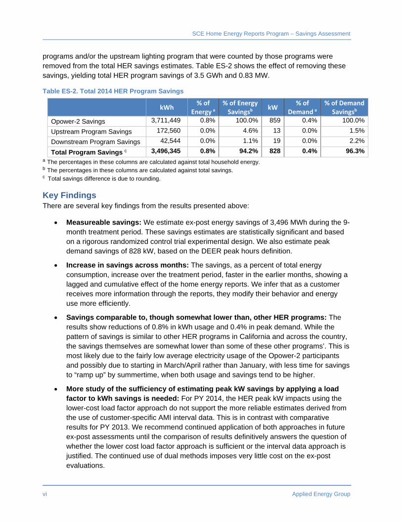
programs and/or the upstream lighting program that were counted by those programs were removed from the total HER savings estimates. Table ES-2 shows the effect of removing these savings, yielding total HER program savings of 3.5 GWh and 0.83 MW.
Table ES-2. Total 2014 HER Program Savings
kWh % of
Energy a% of Energy Savingsb
kW % of
Demand a % of Demand
Savingsb
Opower-2 Savings 3,711,449 0.8% 100.0% 859 0.4% 100.0%
Upstream Program Savings 172,560 0.0% 4.6% 13 0.0% 1.5%
Downstream Program Savings 42,544 0.0% 1.1% 19 0.0% 2.2%
Total Program Savings c 3,496,345 0.8% 94.2% 828 0.4% 96.3%a The percentages in these columns are calculated against total household energy. b The percentages in these columns are calculated against total savings. c Total savings difference is due to rounding.
Key Findings There are several key findings from the results presented above:
Measureable savings: We estimate ex-post energy savings of 3,496 MWh during the 9-month treatment period. These savings estimates are statistically significant and based on a rigorous randomized control trial experimental design. We also estimate peak demand savings of 828 kW, based on the DEER peak hours definition.
Increase in savings across months: The savings, as a percent of total energy consumption, increase over the treatment period, faster in the earlier months, showing a lagged and cumulative effect of the home energy reports. We infer that as a customer receives more information through the reports, they modify their behavior and energy use more efficiently.
Savings comparable to, though somewhat lower than, other HER programs: The results show reductions of 0.8% in kWh usage and 0.4% in peak demand. While the pattern of savings is similar to other HER programs in California and across the country, the savings themselves are somewhat lower than some of these other programs’. This is most likely due to the fairly low average electricity usage of the Opower-2 participants and possibly due to starting in March/April rather than January, with less time for savings to “ramp up” by summertime, when both usage and savings tend to be higher.
More study of the sufficiency of estimating peak kW savings by applying a load factor to kWh savings is needed: For PY 2014, the HER peak kW impacts using the lower-cost load factor approach do not support the more reliable estimates derived from the use of customer-specific AMI interval data. This is in contrast with comparative results for PY 2013. We recommend continued application of both approaches in future ex-post assessments until the comparison of results definitively answers the question of whether the lower cost load factor approach is sufficient or the interval data approach is justified. The continued use of dual methods imposes very little cost on the ex-post evaluations.

Applied Energy Group vii
Table of Contents
Chapter 1 – Introduction ............................................................................................................... 1
Background ............................................................................................................................... 1
Scope of This Savings Assessment .......................................................................................... 1
Report Organization .................................................................................................................. 2
Chapter 2 – Sample Validation ..................................................................................................... 3
Chapter 3 – Analysis Methods for Energy Savings ...................................................................... 5
Overall Analysis Approach ........................................................................................................ 5
Difference in Differences ........................................................................................................... 5
Regression Modeling ................................................................................................................ 6
Data Used in Analysis ............................................................................................................... 8
Chapter 4 – Energy Savings Results ............................................................................................ 9
Difference in Differences Results (Initial kWh Savings Estimates) ........................................... 9
Regression Analysis (Final kWh Savings Estimates) .............................................................. 11
Program-Level Savings ........................................................................................................... 14
Chapter 5 – Peak Demand Impacts ........................................................................................... 15
Load Factor Approach ............................................................................................................ 15
Interval Data Approach ........................................................................................................... 16
Chapter 6 – Attributing Savings to Downstream Programs ........................................................ 19
Chapter 7 – Attributing Savings to Upstream Programs ............................................................. 21
Chapter 8 – Final Results and Key Findings .............................................................................. 25
Appendix A – Fixed-Effects Final Regression Model Output ..................................................... A-1

viii Applied Energy Group
List of Figures
Figure ES-1. Average Per-Participant Energy Savings Estimates and 90% Confidence Intervals ...................................................................................................................................................... v Figure 1. Average Usage of Population by Month ........................................................................ 4 Figure 2. Simplified Regression Modeling Approach ................................................................... 7 Figure 3. Difference in Differences Average Per-Participant 2014 Monthly Energy Use ........... 10 Figure 4. Difference in Differences Average Per-Participant 2014 Monthly Energy Savings Estimates .................................................................................................................................... 10 Figure 5. Regression Analysis Average Per-Participant Monthly Energy Use ........................... 12 Figure 6. Regression Analysis Average Per-Participant kWh Savings Estimates ...................... 12 Figure 7. Average Per-Participant kWh Savings Estimates: Comparison of Regression and Difference in Differences Results ............................................................................................... 13 Figure 8. Monthly kWh Savings Estimates: Percentage Savings, from Final Regression Model 13

Applied Energy Group ix
List of Tables
Table ES-1. Estimated HER 2014 Energy Savings ...................................................................... v Table ES-2. Total 2014 HER Program Savings............................................................................ vi Table 1. Sample Validation for Full Population ............................................................................. 3 Table 2. Customer Attrition ........................................................................................................... 8 Table 3. Monthly Ex-Post Energy Savings Estimates: Difference in Differences ......................... 9 Table 4. Monthly Ex-Post Energy Savings Estimates: Regression Analysis .............................. 11 Table 5. Total HER Program Energy Savings (before adjustment for other program savings) .. 14 Table 6. Comparison of Pre-treatment Summer Average Daily Usage, by Month ..................... 16 Table 7. Downstream Program Savings (kWh) .......................................................................... 19 Table 8. Downstream Program Savings (kW) ............................................................................ 20 Table 9. Total SCE Opower-2 HER Program Savings ............................................................... 25

Applied Energy Group 1
Chapter 1 – Introduction
Background Since December 2012, Opower has operated the Home Energy Report (HER) program, a comparative energy usage and disclosure pilot program, for Southern California Edison in the San Gabriel/Rancho Cucamonga portion of the service territory. This program provides SCE’s residential customers feedback through reports showing household energy use and comparisons of energy use from similar neighbors. The reports also provide a personal comparison, showing the household’s energy usage over time. The reports also give the recipient a number of energy efficiency tips to promote behavior modification in achieving energy savings.
This report documents Applied Energy Group’s evaluation of savings from the Home Energy Report (HER) program that Opower operated for Southern California Edison (SCE) in 2014. As this is the second wave of the HER program, we refer to this program as Opower-2 in this report.
The Opower-2 program targeted residential accounts in the San Gabriel/Rancho Cucamonga portion of SCE‘s service territory. The Home Energy Reports, which compare program participants’ household energy use to that of similar neighbors, were sent out to customers beginning in March 2014 through December 2014. The program operated under a strict randomized control trial experimental design that was reviewed by the CPUC Energy Division. The sample of customers included 150,000 accounts, randomly assigned to one of two equal-sized groups: program participants (treatment or T group) and comparison group (control or C group). The sample was stratified by energy use, with a higher proportion of relatively high electricity use customers included, but also included users of all levels. However, since disproportionally more high usage customers were included in the Opower-1 sample, there were fewer of those customers still available when the Opower-2 sample was selected.
The program ran for the 9 months (mid-March through December 2014) and there were some problems with mismatching of addresses that led to some treatment customers not receiving their HER reports. AEG addressed this situation and other issues in a way consistent with CPUC guidance in estimating the program savings.
Scope of This Savings Assessment This report describes the implementation of the 2014 program, explains our analysis methods, presents detailed energy savings results, and discusses our findings. Our evaluation employed two statistical methodologies to provide ex-post estimates of the HER program savings: We conducted difference in differences analyses to gauge overall energy savings and peak load impacts achieved during the pilot. Then we used regression modeling to refine the energy savings estimate.
The goal was to provide ex-post estimates of savings for the period March-December 2014 that are attributable to the HER program, including:
SCE Home Energy Reports Program – Savings Assessment
2 Applied Energy Group
kWh savings achieved by the program participants, minus their savings claimed by other SCE programs operating during that time;
Peak kW savings calculated two ways, applying a load factor to the kWh savings based on SCE’s load research data and direct estimation from hourly interval data, minus their kW savings claimed by other SCE programs operating during that time.
Report Organization The report is organized as follows:
Chapter 2 describes the sample validation of the Opower-2 population.
Chapter 3 describes the energy savings analysis methods, including the approaches we followed for the difference in differences analysis and the regression modeling.
Chapter 4 presents results from the kWh savings analysis across the program year.
Chapter 5 describes the methods and results of estimating the peak kW savings.
Chapter 6 discusses the attribution of savings to the HER and SCE’s downstream energy efficiency programs.
Chapter 7 discusses the method of attributing savings to the HER and SCE’s upstream lighting program.
Chapter 8 summarizes the findings from our analysis.

Applied Energy Group 3
Chapter 2 – Sample Validation
The estimation of savings requires that the control group provides an accurate representation of the treatment group’s behavior had the home energy reports never been sent. To have confidence in this estimate, the control and treatment groups should be as similar as possible in the pre-treatment period. In combination with a large sample size, the treatment and control group assignments should be random to ensure that, on average, there were no systematic differences between the two groups. The sample population included 150,000 households, with control and treatment groups of equal size.
The sample was stratified by energy use, which enabled us to include proportionally more customers with higher usage, but also include representation at all usage levels. This allowed for the maximization of savings from the available population, since higher use customers tend to save more energy in behavioral programs, but also allows for estimation of savings for more heterogeneous groups by weighting the results by stratum as needed. The participant population was randomly sampled from the broader target population first and then that group was randomly split between treatment and control groups.
To verify the randomization of the control and treatment group sample, we performed a two-sample t-test to determine if there was a significant difference between the two groups. Since the data available to us was limited in terms of identifying characteristics for the customers, we were only able to compare the average daily use during the pre-treatment period between the two groups.
We calculated the average daily kWh use for each customer during the pre-treatment period using the cut-off date of March 18, 2014. This is the start date for generating the customer energy reports. The results of the t-test performed on the entire population are included below. A p-value below 0.05 indicate statistically significant differences. As shown in Table 1, we found no statistically significant difference in the pre-treatment usage between the two groups, as indicated by the p-value of 0.894.
Table 1. Sample Validation for Full Population
Average Daily Electricity Usage (kWh/day)
Group Mean p-value *
Control 20.51 0.894
Treatment 20.51 * Means statistically significant difference
When the program was implemented, there was an issue with mismatched addresses. When the address issue became apparent, a decision was made to not send reports to these addresses. No accounts with mismatched addresses received any of the reports. This address mismatch condition was present in both the treatment group and the control group. It is important to note that the condition had nothing to do with the Opower-2 program – it was inherent in the SCE billing system. Nonetheless, since there was an intent to treat, all of these
SCE Home Energy Reports Program – Savings Assessment
4 Applied Energy Group
treatment and control customers were retained in the dataset and much of the analysis, consistent with the CPUC ED guidance.
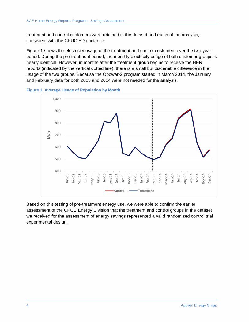
Figure 1 shows the electricity usage of the treatment and control customers over the two year period. During the pre-treatment period, the monthly electricity usage of both customer groups is nearly identical. However, in months after the treatment group begins to receive the HER reports (indicated by the vertical dotted line), there is a small but discernible difference in the usage of the two groups. Because the Opower-2 program started in March 2014, the January and February data for both 2013 and 2014 were not needed for the analysis.
Figure 1. Average Usage of Population by Month
Based on this testing of pre-treatment energy use, we were able to confirm the earlier assessment of the CPUC Energy Division that the treatment and control groups in the dataset we received for the assessment of energy savings represented a valid randomized control trial experimental design.
400
500
600
700
800
900
1,000
Jan‐13
Feb‐13
Mar‐13
Apr‐13
May‐13
Jun‐13
Jul‐13
Aug‐13
Sep‐13
Oct‐13
Nov‐13
Dec‐13
Jan‐14
Feb‐14
Mar‐14
Apr‐14
May‐14
Jun‐14
Jul‐14
Aug‐14
Sep‐14
Oct‐14
Nov‐14
Dec‐14
kWh
Control Treatment
Applied Energy Group 5
Chapter 3 – Analysis Methods for Energy Savings
Overall Analysis Approach To provide an independent estimate of kWh savings from this program, we used two statistical methods: difference in differences and regression analysis. Both make use of pre-treatment and post-treatment monthly billing data for the treatment and control customers that were randomly assigned from the program population at the start of the program, with the mismatched address customers all retained, as described above. First, we used a difference in differences method, which directly estimates the energy savings for each month, along with a standard error and confidence intervals for those savings. Then we refined that direct estimate with a fixed-effects regression model, which also incorporates actual weather data for that same period and reduces variance by accounting for different average energy use across the customers.
Both of these methods provide savings estimates by month along with the associated confidence intervals. The direct estimate from the difference in differences method provides an initial estimate of savings for each month that is not affected by the assumptions of a regression model. Because the regression model includes assumptions about the structure of the data and the nature of the residuals, it helps to have a preliminary estimate to compare with. If the regression model results are comparable to the initial estimates, we can be more confident that the results are valid. Because the regression model incorporates weather and reduces variance by using customer-specific fixed-effects, it will generally provide a more precise estimate than the direct estimate. It also has the advantage that the model can be used to estimate what the savings would have been under different weather scenarios, though estimation of impacts under alternative weather scenarios is not in the scope of this project.
Difference in Differences Equation (1) shows the mathematical calculations used in the difference in differences (DID) analysis to estimate energy savings for each month. In this case, the “before” refers to the pre-treatment month, and the control group is the group that did not receive a report.
Savings Cntl ‐Tx ‐ Cntl ‐Tx (1)
Where
Cntl is the average control group customer energy use in the treatment (after) period
Tx is the average participant group (also referred to as the treatment group) customer energy use in the treatment (after) period
Cntl is the average control group customer energy use in the pre-treatment (before) period
Tx is the average participant group customer energy use in the pre-treatment (before) period
SCE Home Energy Reports Program – Savings Assessment
6 Applied Energy Group
We also calculated standard errors and confidence intervals using the appropriate statistical formulas for the difference of two random variables (estimates).
The DID provides an initial estimate of savings for each month. We did not eliminate the data for opt-out or mismatched address customers from the dataset. The number of customers that opted out was small, the effect of excluding them would have been small, and excluding them could have corrupted the randomization from the experimental design. We also included those customers when expanding the average customer results to the total population, so they were treated consistently.
Regression Modeling We next estimated savings using a fixed-effect regression model. Both treatment and control customers are included in the model, which includes variables related to participation and weather. The model also includes a fixed effect for each customer, which is a customer-specific intercept.
The fixed-effects regression approach controls for unmeasured differences between customers that are constant over time, such as home size, vintage, major appliances, and household size, allowing us to better isolate and estimate the energy use changes associated with program participation (the savings) more precisely. We use a standard fixed-effects (also known as panel) regression, and use robust errors to reflect the correlation of the errors in the model.
The independent variables investigated are as follows:
Temperature (cooling degree days and heating degree days)
Treatment period year and month – to account for any changes in customer energy use over time that is not related to the program
Participation (set for treatment customers during the treatment period)
The model looks at the dependent variable (monthly energy use) as a function of the other independent or explanatory variables and then estimates the coefficients of the variables in that function.
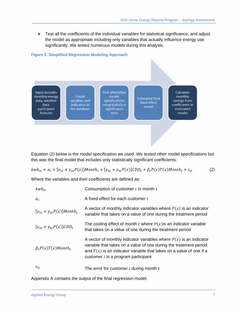
In general, our regression analysis included the following general steps and assumptions (Figure 2 illustrates the approach):
Create variables and indicators in the database. Note: The independent variables investigated include some that are related to participation, and others that are not. Conceptually, information not related to participation goes into the model to estimate the baseline energy use based on all customers (including treatment and control group customers), while the participation variables estimate the program impacts.
Run the fixed-effects model using all treatment and control group customers to estimate the baseline energy use and the savings for the actual analysis period and for different scenarios as needed using the model coefficients.
SCE Home Energy Reports Program – Savings Assessment
Applied Energy Group 7
Test all the coefficients of the individual variables for statistical significance, and adjust the model as appropriate including only variables that actually influence energy use significantly. We tested numerous models during this analysis.
Figure 2. Simplified Regression Modeling Approach
Equation (2) below is the model specification we used. We tested other model specifications but this was the final model that includes only statistically significant coefficients.
(2)
Where the variables and their coefficients are defined as:
Consumption of customer in month
A fixed effect for each customer
A vector of monthly indicator variables where is an indicator variable that takes on a value of one during the treatment period
The cooling effect of month where is an indicator variable that takes on a value of one during the treatment period
A vector of monthly indicator variables where is an indicator variable that takes on a value of one during the treatment period and is an indicator variable that takes on a value of one if a customer is a program participant
The error for customer during month
Appendix A contains the output of the final regression model.

SCE Home Energy Reports Program – Savings Assessment
8 Applied Energy Group
Data Used in Analysis We conducted the energy analysis using monthly energy data for the pre-treatment and treatment periods. We used monthly billing data for the period of March through December for both 2013 and 2014. The treatment period began on March 18, 2015, when the first HER reports were sent out. We excluded all January and February 2014 bills, and those March bills with a billing period that ended before March 18 from the analysis because they preceded the mailing of the first reports for this program, and so could not have had any program-related savings. We excluded the same months for 2013 to ensure that the two periods were consistent.
When we calculated the savings estimates and their statistical significance, we found that the savings estimate for March was not statistically significant in either the difference in differences analysis or the regression analysis. This is not surprising, given that the March bills only included a partial month of usage after the reports were sent out, and so there was not much time for customers to take actions or for savings to accumulate over time. Because they were not statistically significant, the March estimates were not included in the total savings.
For participants and control group customers who moved out of their homes during 2014, we included energy data up until the time they left.
Table 2 illustrates the customer attrition due to customers who moved out during the treatment period of the study. The table shows the count of households that had available data for the treatment and control groups by month. The number of closed accounts is tracked by month and cumulatively.
Table 2. Customer Attrition
Month
Control Group Treatment Group
Open Accountsa
Closed Accounts Open Accountsa
Closed Accounts
Monthly Cumulative Monthly Cumulative
Mar 2014 73,881 1,119 1,119 73,786 1,214 1,214
Apr 2014 73,551 330 1,449 73,472 314 1,528
May 2014 73,265 286 1,735 73,169 303 1,831
Jun 2014 72,915 350 2,085 72,847 322 2,153
Jul 2014 72,489 426 2,511 72,427 420 2,573
Aug 2014 72,118 371 2,882 72,087 340 2,913
Sep 2014 71,795 323 3,205 71,784 303 3,216
Oct 2014 71,384 411 3,616 71,415 369 3,585
Nov 2014 71,076 308 3,924 71,138 277 3,862
Dec 2014 70,794 282 4,206 70,833 305 4,167 a Count of number of customer accounts varies by month due to account closure.
Applied Energy Group 9
Chapter 4 – Energy Savings Results
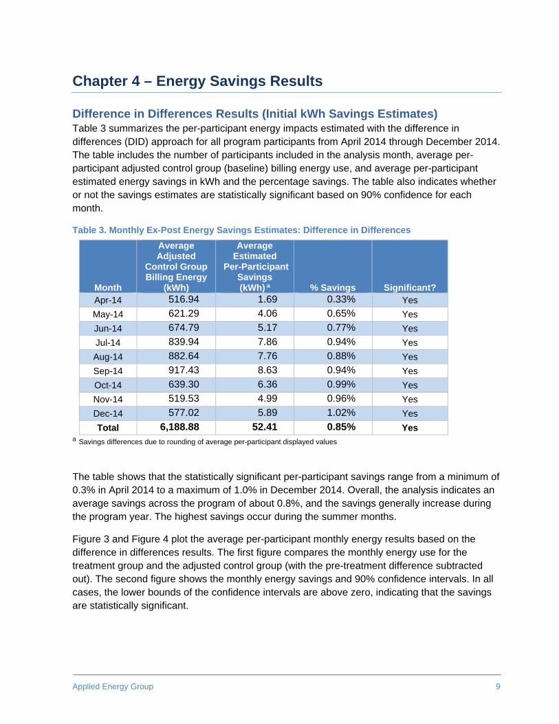
Difference in Differences Results (Initial kWh Savings Estimates) Table 3 summarizes the per-participant energy impacts estimated with the difference in differences (DID) approach for all program participants from April 2014 through December 2014. The table includes the number of participants included in the analysis month, average per-participant adjusted control group (baseline) billing energy use, and average per-participant estimated energy savings in kWh and the percentage savings. The table also indicates whether or not the savings estimates are statistically significant based on 90% confidence for each month.
Table 3. Monthly Ex-Post Energy Savings Estimates: Difference in Differences
Month
Average Adjusted
Control Group Billing Energy
(kWh)
Average Estimated
Per-Participant Savings (kWh) a % Savings Significant?
Apr-14 516.94 1.69 0.33% Yes
May-14 621.29 4.06 0.65% Yes
Jun-14 674.79 5.17 0.77% Yes
Jul-14 839.94 7.86 0.94% Yes
Aug-14 882.64 7.76 0.88% Yes
Sep-14 917.43 8.63 0.94% Yes
Oct-14 639.30 6.36 0.99% Yes
Nov-14 519.53 4.99 0.96% Yes
Dec-14 577.02 5.89 1.02% Yes
Total 6,188.88 52.41 0.85% Yes a Savings differences due to rounding of average per-participant displayed values
The table shows that the statistically significant per-participant savings range from a minimum of 0.3% in April 2014 to a maximum of 1.0% in December 2014. Overall, the analysis indicates an average savings across the program of about 0.8%, and the savings generally increase during the program year. The highest savings occur during the summer months.
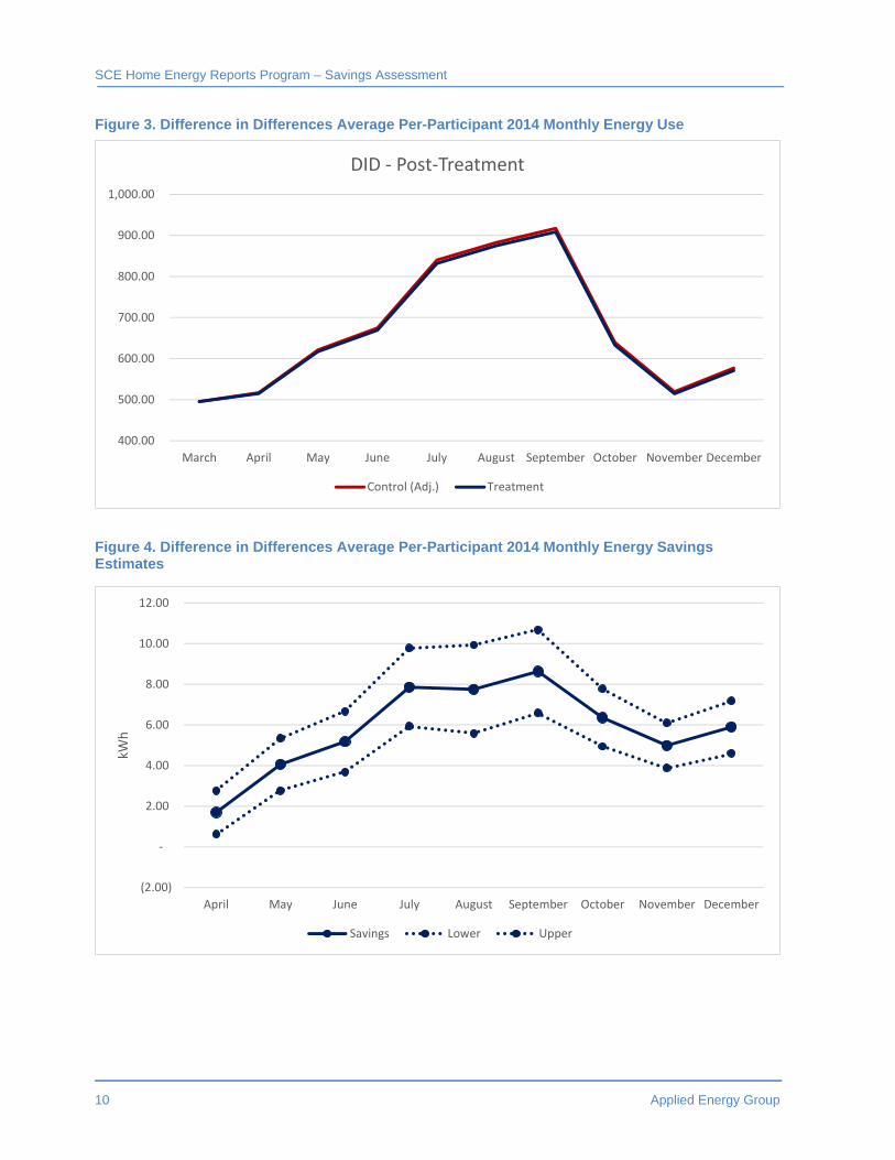
Figure 3 and Figure 4 plot the average per-participant monthly energy results based on the difference in differences results. The first figure compares the monthly energy use for the treatment group and the adjusted control group (with the pre-treatment difference subtracted out). The second figure shows the monthly energy savings and 90% confidence intervals. In all cases, the lower bounds of the confidence intervals are above zero, indicating that the savings are statistically significant.
SCE Home Energy Reports Program – Savings Assessment
10 Applied Energy Group
Figure 3. Difference in Differences Average Per-Participant 2014 Monthly Energy Use
Figure 4. Difference in Differences Average Per-Participant 2014 Monthly Energy Savings Estimates
400.00
500.00
600.00
700.00
800.00
900.00
1,000.00
March April May June July August September October November December
DID ‐ Post‐Treatment
Control (Adj.) Treatment
(2.00)
‐
2.00
4.00
6.00
8.00
10.00
12.00
April May June July August September October November December
kWh
Savings Lower Upper
SCE Home Energy Reports Program – Savings Assessment
Applied Energy Group 11
Regression Analysis (Final kWh Savings Estimates) After estimating the savings using a difference in differences, we then estimated the savings using a fixed-effects regression model. The first step in the assessment of the regression model was to check the results for consistency against the results from the difference in differences analysis. We found that the results were similar and, as expected, the results of from the regression model are somewhat more precise. We used the regression model results to make the final program-level estimates presented at the end of this chapter.
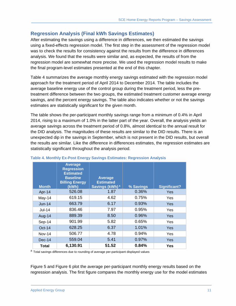
Table 4 summarizes the average monthly energy savings estimated with the regression model approach for the treatment period of April 2014 to December 2014. The table includes the average baseline energy use of the control group during the treatment period, less the pre-treatment difference between the two groups, the estimated treatment customer average energy savings, and the percent energy savings. The table also indicates whether or not the savings estimates are statistically significant for the given month.
The table shows the per-participant monthly savings range from a minimum of 0.4% in April 2014, rising to a maximum of 1.0% in the latter part of the year. Overall, the analysis yields an average savings across the treatment period of 0.8%, almost identical to the annual result for the DID analysis. The magnitudes of these results are similar to the DID results. There is an unexpected dip in the savings in September, which is not present in the DID results, but overall the results are similar. Like the difference in differences estimates, the regression estimates are statistically significant throughout the analysis period.
Table 4. Monthly Ex-Post Energy Savings Estimates: Regression Analysis
Month
Average Regression Estimated Baseline
Billing Energy (kWh)
Average Estimated
Savings (kWh) a % Savings Significant? Apr-14 526.08 1.87 0.36% Yes
May-14 619.15 4.62 0.75% Yes
Jun-14 663.79 6.17 0.93% Yes
Jul-14 836.46 7.97 0.95% Yes
Aug-14 889.39 8.50 0.96% Yes
Sep-14 901.99 5.82 0.65% Yes
Oct-14 628.25 6.37 1.01% Yes
Nov-14 506.77 4.78 0.94% Yes
Dec-14 559.04 5.41 0.97% Yes
Total 6,130.91 51.52 0.84% Yes a Total savings differences due to rounding of average per-participant displayed values
Figure 5 and Figure 6 plot the average per-participant monthly energy results based on the regression analysis. The first figure compares the monthly energy use for the model estimates

SCE Home Energy Reports Program – Savings Assessment
12 Applied Energy Group
of the treatment and control groups. The second figure shows the monthly energy savings and 90% confidence intervals. In all cases, the lower bounds of the confidence intervals are above zero, indicating that the savings are still statistically significant.
Figure 5. Regression Analysis Average Per-Participant Monthly Energy Use
Figure 6. Regression Analysis Average Per-Participant kWh Savings Estimates
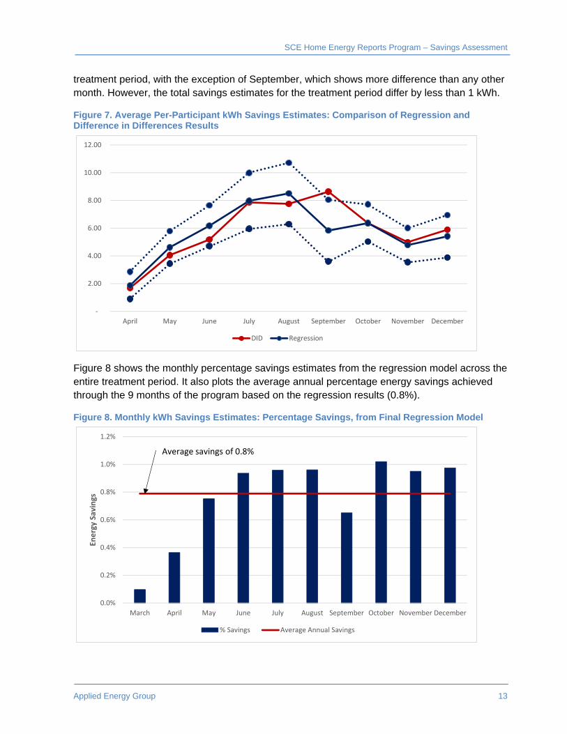
Figure 7 compares the monthly energy savings estimated with the regression model and the difference in differences approach. The energy savings are very similar across the whole
400
500
600
700
800
900
1,000
April May June July August September October November December
kWh
Predicted Load Treatment
(2.00)
‐
2.00
4.00
6.00
8.00
10.00
12.00
April May June July August September October November December
kWh
Savings Lower Upper
SCE Home Energy Reports Program – Savings Assessment
Applied Energy Group 13
treatment period, with the exception of September, which shows more difference than any other month. However, the total savings estimates for the treatment period differ by less than 1 kWh.
Figure 7. Average Per-Participant kWh Savings Estimates: Comparison of Regression and Difference in Differences Results
Figure 8 shows the monthly percentage savings estimates from the regression model across the entire treatment period. It also plots the average annual percentage energy savings achieved through the 9 months of the program based on the regression results (0.8%).
Figure 8. Monthly kWh Savings Estimates: Percentage Savings, from Final Regression Model
‐
2.00
4.00
6.00
8.00
10.00
12.00
April May June July August September October November December
DID Regression
0.0%
0.2%
0.4%
0.6%
0.8%
1.0%
1.2%
March April May June July August September October November December
Energy Savings
% Savings Average Annual Savings
Average savings of 0.8%
SCE Home Energy Reports Program – Savings Assessment
14 Applied Energy Group
Program-Level Savings The results from both the difference in differences model and the regression model show similar savings estimates. Because they are more precise, we use the regression model results to calculate program-level savings.
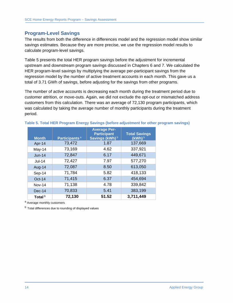
Table 5 presents the total HER program savings before the adjustment for incremental upstream and downstream program savings discussed in Chapters 6 and 7. We calculated the HER program-level savings by multiplying the average per-participant savings from the regression model by the number of active treatment accounts in each month. This gave us a total of 3.71 GWh of savings, before adjusting for the savings from other programs.
The number of active accounts is decreasing each month during the treatment period due to customer attrition, or move-outs. Again, we did not exclude the opt-out or mismatched address customers from this calculation. There was an average of 72,130 program participants, which was calculated by taking the average number of monthly participants during the treatment period.
Table 5. Total HER Program Energy Savings (before adjustment for other program savings)
Month Participants a
Average Per-Participant
Savings (kWh) b Total Savings
(kWh) b Apr-14 73,472 1.87 137,669
May-14 73,169 4.62 337,921
Jun-14 72,847 6.17 449,671
Jul-14 72,427 7.97 577,270
Aug-14 72,087 8.50 613,050
Sep-14 71,784 5.82 418,133
Oct-14 71,415 6.37 454,694
Nov-14 71,138 4.78 339,842
Dec-14 70,833 5.41 383,199
Total b 72,130 51.52 3,711,449 a Average monthly customers b Total differences due to rounding of displayed values
Applied Energy Group 15
Chapter 5 – Peak Demand Impacts
We conducted two analyses to assess the peak kW impacts of the Opower-2 program. We made one estimate by applying an average residential class load factor to the estimated kWh savings. We also developed an estimate using interval data from the actual participants that was analogous to the way we estimated the difference in differences energy savings. We used the 3-day heat wave as defined by DEER for both estimates.
The revised savings estimate, based on actual customer interval data for the program year and the DEER peak definition, captures behavior at the peak period in 2014 and represents our final result for peak load savings for the Opower-2 program.
Load Factor Approach Once we estimated the kWh savings, we then calculated a preliminary estimate of kW savings using SCE’s Dynamic Load Profiles (DLP), reweighted to better reflect the makeup of the SCE HER population. We used these load profiles to develop a load factor for the peak hours, which we then applied to the kWh savings to obtain a rough estimate of the kW savings.
The SCE’s dynamic load profiles are based on a stratified sample representing the entire SCE residential population, with stratification based on average monthly energy use, climate zone, and housing type (single family and multifamily). We calculated new weights based on the distribution of customers in the Opower-2 population across the strata defined by the DLP sample. By applying these alternative weights to the DLP sample interval data, SCE’s Load Research department recalculated an annual 8,760-hour load shape that reflected the customers in the Opower-2 participant population.
Using this reweighted 8,760-hour load shape and the 2014 DEER-defined 3-day heat wave, which is September 15-17, 2014 for the climate zones included in the participant population1, we calculated the average kW for the three peak hours from 2:00-5:00 PM on each of the three days. Using that average peak kW, we calculated the peak load factor as the ratio of the annual consumption to the product of the peak demand and the number of hours (8,760). The peak load factor based on the reweighted dynamic load profile using this approach was 42.59%.
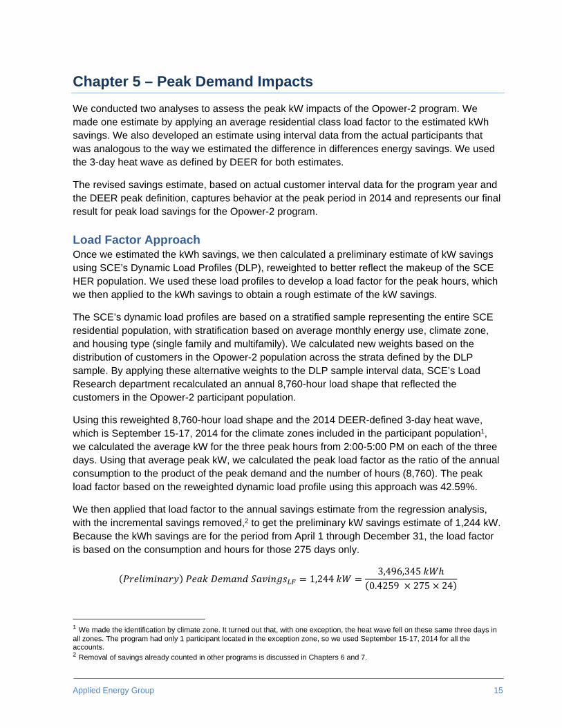
We then applied that load factor to the annual savings estimate from the regression analysis, with the incremental savings removed,2 to get the preliminary kW savings estimate of 1,244 kW. Because the kWh savings are for the period from April 1 through December 31, the load factor is based on the consumption and hours for those 275 days only.
1,2443,496,345
0.4259 275 24
1 We made the identification by climate zone. It turned out that, with one exception, the heat wave fell on these same three days in all zones. The program had only 1 participant located in the exception zone, so we used September 15-17, 2014 for all the accounts. 2 Removal of savings already counted in other programs is discussed in Chapters 6 and 7.
SCE Home Energy Reports Program – Savings Assessment
16 Applied Energy Group
In the following section, we discuss the improved savings estimate of the peak demand impacts using actual interval data.
Interval Data Approach We also developed a kW savings estimate based on the actual treatment and control group customer interval data to give an improved savings estimate that more directly represents the savings for these customers. SCE provided hourly interval data for 2013 and 2014 summer months, for both treatment and control group customers.
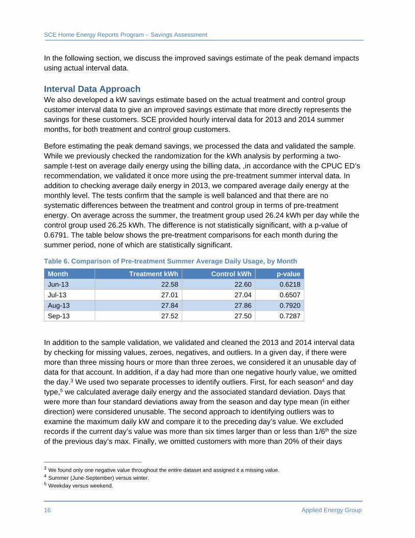
Before estimating the peak demand savings, we processed the data and validated the sample. While we previously checked the randomization for the kWh analysis by performing a two-sample t-test on average daily energy using the billing data, ,in accordance with the CPUC ED’s recommendation, we validated it once more using the pre-treatment summer interval data. In addition to checking average daily energy in 2013, we compared average daily energy at the monthly level. The tests confirm that the sample is well balanced and that there are no systematic differences between the treatment and control group in terms of pre-treatment energy. On average across the summer, the treatment group used 26.24 kWh per day while the control group used 26.25 kWh. The difference is not statistically significant, with a p-value of 0.6791. The table below shows the pre-treatment comparisons for each month during the summer period, none of which are statistically significant.
Table 6. Comparison of Pre-treatment Summer Average Daily Usage, by Month
Month Treatment kWh Control kWh p-value
Jun-13 22.58 22.60 0.6218
Jul-13 27.01 27.04 0.6507
Aug-13 27.84 27.86 0.7920
Sep-13 27.52 27.50 0.7287
In addition to the sample validation, we validated and cleaned the 2013 and 2014 interval data by checking for missing values, zeroes, negatives, and outliers. In a given day, if there were more than three missing hours or more than three zeroes, we considered it an unusable day of data for that account. In addition, if a day had more than one negative hourly value, we omitted the day.3 We used two separate processes to identify outliers. First, for each season4 and day type,5 we calculated average daily energy and the associated standard deviation. Days that were more than four standard deviations away from the season and day type mean (in either direction) were considered unusable. The second approach to identifying outliers was to examine the maximum daily kW and compare it to the preceding day’s value. We excluded records if the current day’s value was more than six times larger than or less than 1/6th the size of the previous day’s max. Finally, we omitted customers with more than 20% of their days
3 We found only one negative value throughout the entire dataset and assigned it a missing value. 4 Summer (June-September) versus winter. 5 Weekday versus weekend.

SCE Home Energy Reports Program – Savings Assessment
Applied Energy Group 17
flagged as unusable. Overall, the SCE data were quite clean. In total, the exclusions from the cleaning amounted to just under 1% of the records.
For the interval data approach, we used exactly the same DEER defined heat wave dates as the load factor approach. The average per-participant peak savings is 0.0120 kW. This is a savings of 0.43% from baseline demand. The 90% confidence interval is +/- 0.0102 kW.
Finally, we calculated the aggregate (program-level) kW impact. We did this by taking the average per-participant savings estimate and multiplying it by the number of participants as of September 15, 2014, which was 71,599. To calculate the final peak demand savings estimate, we removed the savings associated with and already counted in other programs, 18.94 kW from downstream and 12.55 kW from upstream programs, to avoid double counting.6 Thus, the interval data approach yields a kW impact estimate of 827.70 kW.
827.70 0.012 71,599 859.19 18.94 12.55
The result from the analysis of interval data, 804 kW, is our final estimate of the kW savings associated with the Opower-2 program.
One of the ancillary objectives of this analysis was to assess the two alternative methods of estimating peak kW savings. The question is: do the Load Factor approach and Interval Data approach consistently yield sufficiently close results to instill confidence in the lower cost method? The LF approach costs considerably less to implement since it does not require the assembly and analysis of very large advanced metering infrastructure (AMI) interval data files. The key difference between the two methods is that the LF method assumes no change in the load shape—i.e., the savings are proportionally distributed across all hours, while the Interval Data approach allows the savings to vary freely across hours of the day. In this analysis, we found that the LF approach produced peak load savings notably higher than the Interval Data approach. So for PY 2014, unlike PY 2013, we do not believe that the less expensive method is sufficient, and we use the interval data approach to estimate savings. Since the LF approach adds very little cost to the ex-post evaluation, however, we encourage continuation of both methods for a few more program years before drawing a final conclusion.
6 Calculation of savings from the downstream and upstream programs is discussed in the following chapters. The values are included here to allow direct comparison of kW savings estimates using the load factor and interval data approaches, since the load factor approach inherently includes the removal of double counted savings.

Applied Energy Group 19
Chapter 6 – Attributing Savings to Downstream Programs
SCE provided AEG with the annual per-measure net savings estimates for HER participant and control group customers’ participation in other energy efficiency programs the company offered in 2014, from the savings data submitted to CPUC. These programs are referred to as downstream programs because incentives are offered directly to the end-users of energy and their participation and expected savings are tracked by individual households.
A wide range of energy efficiency measures are rebated through these programs. Because SCE receives credit for the savings achieved through these programs, it is possible that part of the total 2014 HER savings estimated and reported in the previous chapters are attributable to and were counted as part of those downstream programs’ savings. Note that it is only the incremental difference in savings between the treatment and control group customers that are at risk of double counting – the control group accounts form a “baseline” level of participation that would have happened in the absence of the Opower-2 program.
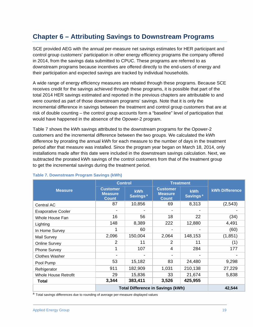
Table 7 shows the kWh savings attributed to the downstream programs for the Opower-2 customers and the incremental difference between the two groups. We calculated the kWh difference by prorating the annual kWh for each measure to the number of days in the treatment period after that measure was installed. Since the program year began on March 18, 2014, only installations made after this date were included in the downstream savings calculation. Next, we subtracted the prorated kWh savings of the control customers from that of the treatment group to get the incremental savings during the treatment period.
Table 7. Downstream Program Savings (kWh)
Measure
Control Treatment
kWh Difference Customer Measure
Count
kWh Savings a
Customer Measure
Count
kWh Savings a
Central AC 87 10,856 69 8,313 (2,543)
Evaporative Cooler - - - - -
Whole House Fan 16 56 18 22 (34)
Lighting 148 8,389 222 12,880 4,491
In Home Survey 1 60 - - (60)
Mail Survey 2,096 150,004 2,064 148,153 (1,851)
Online Survey 2 11 2 11 (1)
Phone Survey 1 107 4 284 177
Clothes Washer - - - - -
Pool Pump 53 15,182 83 24,480 9,298
Refrigerator 911 182,909 1,031 210,138 27,229
Whole House Retrofit 29 15,836 33 21,674 5,838 Total 3,344 383,411 3,526 425,955
Total Difference in Savings (kWh) 42,544 a Total savings differences due to rounding of average per-measure displayed values
SCE Home Energy Reports Program – Savings Assessment
20 Applied Energy Group
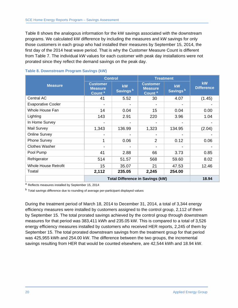
Table 8 shows the analogous information for the kW savings associated with the downstream programs. We calculated kW difference by including the measures and kW savings for only those customers in each group who had installed their measures by September 15, 2014, the first day of the 2014 heat wave period. That is why the Customer Measure Count is different from Table 7. The individual kW values for each customer with peak day installations were not prorated since they reflect the demand savings on the peak day.
Table 8. Downstream Program Savings (kW)
Measure
Control Treatment kW
Difference Customer Measure Count a
kW Savings b
Customer Measure Count a
kW Savings b
Central AC 41 5.52 30 4.07 (1.45) Evaporative Cooler - - - - - Whole House Fan 14 0.04 15 0.04 0.00 Lighting 143 2.91 220 3.96 1.04 In Home Survey - - - - - Mail Survey 1,343 136.99 1,323 134.95 (2.04) Online Survey - - - - - Phone Survey 1 0.06 2 0.12 0.06 Clothes Washer - - - - - Pool Pump 41 2.88 66 3.73 0.85
Refrigerator 514 51.57 568 59.60 8.02
Whole House Retrofit 15 35.07 21 47.53 12.46 Toatal 2,112 235.05 2,245 254.00
Total Difference in Savings (kW) 18.94 a Reflects measures installed by September 15, 2014 b Total savings difference due to rounding of average per-participant displayed values
During the treatment period of March 18, 2014 to December 31, 2014, a total of 3,344 energy efficiency measures were installed by customers assigned to the control group, 2,112 of them by September 15. The total prorated savings achieved by the control group through downstream measures for that period was 383,411 kWh and 235.05 kW. This is compared to a total of 3,526 energy efficiency measures installed by customers who received HER reports, 2,245 of them by September 15. The total prorated downstream savings from the treatment group for that period was 425,955 kWh and 254.00 kW. The difference between the two groups, the incremental savings resulting from HER that would be counted elsewhere, are 42,544 kWh and 18.94 kW.

Applied Energy Group 21
Chapter 7 – Attributing Savings to Upstream Programs
Upstream program savings are not tracked at the customer level, but are also a source of savings that can potentially be double counted by the HER program. SCE runs a program that provides incentives to manufacturers and retailers to change stocking practices of energy efficient CFLs and LEDs (Upstream Lighting Program or ULP). Since it is not possible to track which customers purchased bulbs at reduced prices, we used the proxy method developed in consultation with the CPUC ED to determine the savings that are potentially double-counted. While we are using the method as agreed to for this year’s savings, we do intend to revisit this next year and investigate how we might adjust the approach to better reflect the situation at SCE. It may be appropriate to modify the approach to reflect differences in the implementation of upstream lighting programs and HER programs at SCE.
PG&E conducted in-home surveys7 that assess the uptake of upstream measures (mainly, CFLs and flat screen TVs). The surveys included samples of treatment and control customers from PG&E’s HER program. The CPUC ED has supported the use of these results for SCE, rather than duplicate that very costly and time-consuming study. This is also consistent with more recent lighting analysis memos produced by TRC.8 The method assumes the same per-participant change in bulb installations (also referred to as “excess bulbs” below) resulting from HER participation for SCE as PG&E, and uses the results from that study as the basis for the estimate of the SCE upstream incremental savings.
In the PG&E survey report (and incorporated in the TRC memo), the analysis identified that, on average, treatment households installed an additional 0.95 energy efficient bulbs9 per household more than the control group. The TRC memo estimated that 72% of these bulbs were CFL and the balance, 28%, were LEDs – or 0.68 and 0.27 bulbs per household, respectively.10 As with the downstream savings described in the previous chapter, it is only the incremental difference between the treatment and control groups that would potentially be double counted. To reiterate, the assumption made in the use of the PG&E home study is that the increase in per customer lamp purchases resulting from receiving HERs is the same for the programs at the two different utilities. The additional bulbs per customer represent savings that could be potentially be counted by both the ULP and the Opower-2 program.
To calculate the Opower-2 customers who might have made installations, we made the additional assumption, consistent with the TRC proposed changes memo, that all the CFLs and LEDS were installed evenly (one-twelfth per month) throughout the first year. Since the Opower-2 program savings analysis described in previous chapters only includes savings starting in April, we reduced the excess bulbs by 25% to remove January-March. We then applied the
7 Freeman, Sullivan & Co, “Evaluation of Pacific Gas and Electric Company's Home Energy Report Initiative for the 2010–2012 Program,” April 25, 2012. (aka PG&E home inventory study) 8 TRC Solutions, “Lighting Savings Overlap in 2014 IOU Residential Behavioral Programs,” June 30, 2015 and maintained in October 22, 2015 revision cited below. 9 Op cit, Freeman, Sullivan & Co, Table 7-3, p. 46. Surveys conducted in PG&E service territory; no data for SCE service territory available. Also used in TRC memo. 10 TRC Solutions, “Proposed Changes to Draft ULP HER Lighting Savings Overlap for 2014,” October 22, 2015, p. 5.

SCE Home Energy Reports Program – Savings Assessment
22 Applied Energy Group
straight-line ramp from April to December to the average of the April-December participants, or 68,396 customers. We arrived at the total count of customers by removing both closed and address mismatched accounts from the total. This is the only place where we removed mismatched accounts in the entire study, in line with the TRC memo.11
The next step was determining what fraction of the savings for the additional bulbs are also counted as part of the ULP. According to the TRC work, a ratio of 0.4 of CFLs and 0.2 of LEDs received rebates statewide through the ULP, calculated as the total rebated CFLs divided by the total CFLs sold, and the same holding true for LEDs. Next, we determined the fraction of rebated CFLs and LEDs attributable to the ULP using the applicable net-to-gross ratio (NTGR). For the SCE territory, the most recent, approved upstream lighting net-to-gross ratio is 0.69.
The final step was determining the expected total energy savings per year, based on the average hours of use per day and the average wattage saved per CFL and per LED. Based on information for SCE in the ULP report, the typical ULP CFL light bulb saves 45.2 kWh/year and the typical LED light bulb saves 19.9 kWh/year (compared to a CFL).
Multiplying all of these values together (shown below) gives us the respective CFL and LED incremental savings that need to be deducted from the total annual Opower-2 kWh savings estimate. Unless otherwise noted, the input values come from the TRC memos.12
0.95 Excess Bulbs (based on PG&E Home Inventory)
× 0.72 Fraction of Excess Bulbs sold that were CFLs
× 0.75 Fraction of Year program was running
× 0.97 Installation rate of rebated CFLs
× 68,396 Opower-2 HER customers13
× 0.375 Proration of full year savings to program year savings14
× 0.4 Proportion of CFLs that are rebated (statewide)
× 0.69 Proportion of CFLs attributable to upstream program (SCE specific)
× 45.2 Per CFL savings per year (SCE specific)
= 158,84715 CFL kWh of savings attributable to both programs
11 Op cit, TRC Solutions, June 30, 2015. 12 Op cit, TRC Solutions, June 30 and October 22, 2015. 13 Average number of customers from April-December of 2014 after removing Mismatched and Inactive accounts. 14 Calculated as one half of the 9 months of the program, since the ramp up is assumed to be continuous throughout the first year. 15 Different from the displayed numbers above due to rounding.
SCE Home Energy Reports Program – Savings Assessment
Applied Energy Group 23
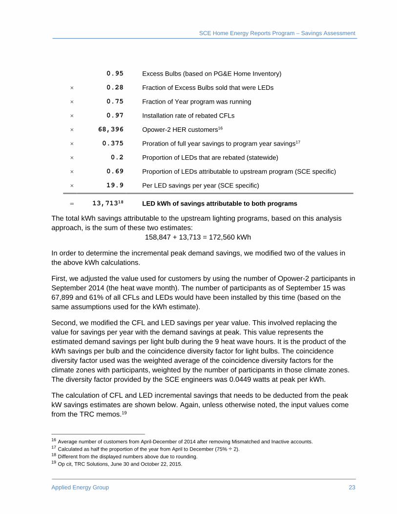
0.95 Excess Bulbs (based on PG&E Home Inventory)
× 0.28 Fraction of Excess Bulbs sold that were LEDs
× 0.75 Fraction of Year program was running
× 0.97 Installation rate of rebated CFLs
× 68,396 Opower-2 HER customers16
× 0.375 Proration of full year savings to program year savings17
× 0.2 Proportion of LEDs that are rebated (statewide)
× 0.69 Proportion of LEDs attributable to upstream program (SCE specific)
× 19.9 Per LED savings per year (SCE specific)
= 13,71318 LED kWh of savings attributable to both programs
The total kWh savings attributable to the upstream lighting programs, based on this analysis approach, is the sum of these two estimates: 158,847 + 13,713 = 172,560 kWh
In order to determine the incremental peak demand savings, we modified two of the values in the above kWh calculations.
First, we adjusted the value used for customers by using the number of Opower-2 participants in September 2014 (the heat wave month). The number of participants as of September 15 was 67,899 and 61% of all CFLs and LEDs would have been installed by this time (based on the same assumptions used for the kWh estimate).
Second, we modified the CFL and LED savings per year value. This involved replacing the value for savings per year with the demand savings at peak. This value represents the estimated demand savings per light bulb during the 9 heat wave hours. It is the product of the kWh savings per bulb and the coincidence diversity factor for light bulbs. The coincidence diversity factor used was the weighted average of the coincidence diversity factors for the climate zones with participants, weighted by the number of participants in those climate zones. The diversity factor provided by the SCE engineers was 0.0449 watts at peak per kWh.
The calculation of CFL and LED incremental savings that needs to be deducted from the peak kW savings estimates are shown below. Again, unless otherwise noted, the input values come from the TRC memos.19
16 Average number of customers from April-December of 2014 after removing Mismatched and Inactive accounts. 17 Calculated as half the proportion of the year from April to December (75% ÷ 2). 18 Different from the displayed numbers above due to rounding. 19 Op cit, TRC Solutions, June 30 and October 22, 2015.
SCE Home Energy Reports Program – Savings Assessment
24 Applied Energy Group
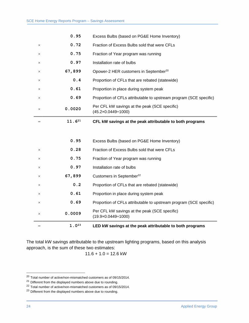
0.95 Excess Bulbs (based on PG&E Home Inventory)
× 0.72 Fraction of Excess Bulbs sold that were CFLs
× 0.75 Fraction of Year program was running
× 0.97 Installation rate of bulbs
× 67,899 Opower-2 HER customers in September20
× 0.4 Proportion of CFLs that are rebated (statewide)
× 0.61 Proportion in place during system peak
× 0.69 Proportion of CFLs attributable to upstream program (SCE specific)
× 0.0020 Per CFL kW savings at the peak (SCE specific) (45.2×0.0449÷1000)
= 11.621 CFL kW savings at the peak attributable to both programs
0.95 Excess Bulbs (based on PG&E Home Inventory)
× 0.28 Fraction of Excess Bulbs sold that were CFLs
× 0.75 Fraction of Year program was running
× 0.97 Installation rate of bulbs
× 67,899 Customers in September22
× 0.2 Proportion of CFLs that are rebated (statewide)
× 0.61 Proportion in place during system peak
× 0.69 Proportion of CFLs attributable to upstream program (SCE specific)
× 0.0009 Per CFL kW savings at the peak (SCE specific) (19.9×0.0449÷1000)
= 1.023 LED kW savings at the peak attributable to both programs
The total kW savings attributable to the upstream lighting programs, based on this analysis approach, is the sum of these two estimates: 11.6 + 1.0 = 12.6 kW
20 Total number of active/non-mismatched customers as of 09/15/2014. 21 Different from the displayed numbers above due to rounding. 22 Total number of active/non-mismatched customers as of 09/15/2014. 23 Different from the displayed numbers above due to rounding.
Applied Energy Group 25
Chapter 8 – Final Results and Key Findings
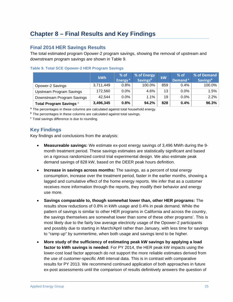
Final 2014 HER Savings Results The total estimated program Opower-2 program savings, showing the removal of upstream and downstream program savings are shown in Table 9.
Table 9. Total SCE Opower-2 HER Program Savings
kWh % of
Energy a% of Energy Savingsb
kW % of
Demand a % of Demand
Savingsb
Opower-2 Savings 3,711,449 0.8% 100.0% 859 0.4% 100.0%
Upstream Program Savings 172,560 0.0% 4.6% 13 0.0% 1.5%
Downstream Program Savings 42,544 0.0% 1.1% 19 0.0% 2.2%
Total Program Savings c 3,496,345 0.8% 94.2% 828 0.4% 96.3%a The percentages in these columns are calculated against total household energy. b The percentages in these columns are calculated against total savings. c Total savings difference is due to rounding.
Key Findings Key findings and conclusions from the analysis:
Measureable savings: We estimate ex-post energy savings of 3,496 MWh during the 9-month treatment period. These savings estimates are statistically significant and based on a rigorous randomized control trial experimental design. We also estimate peak demand savings of 828 kW, based on the DEER peak hours definition.
Increase in savings across months: The savings, as a percent of total energy consumption, increase over the treatment period, faster in the earlier months, showing a lagged and cumulative effect of the home energy reports. We infer that as a customer receives more information through the reports, they modify their behavior and energy use more.
Savings comparable to, though somewhat lower than, other HER programs: The results show reductions of 0.8% in kWh usage and 0.4% in peak demand. While the pattern of savings is similar to other HER programs in California and across the country, the savings themselves are somewhat lower than some of these other programs’. This is most likely due to the fairly low average electricity usage of the Opower-2 participants and possibly due to starting in March/April rather than January, with less time for savings to “ramp up” by summertime, when both usage and savings tend to be higher.
More study of the sufficiency of estimating peak kW savings by applying a load factor to kWh savings is needed: For PY 2014, the HER peak kW impacts using the lower-cost load factor approach do not support the more reliable estimates derived from the use of customer-specific AMI interval data. This is in contrast with comparative results for PY 2013. We recommend continued application of both approaches in future ex-post assessments until the comparison of results definitively answers the question of
SCE Home Energy Reports Program – Savings Assessment
26 Applied Energy Group
whether the lower cost load factor approach is sufficient or the interval data approach is justified. The continued use of dual methods imposes very little cost on the ex-post evaluations.

Appendix

Applied Energy Group A-1
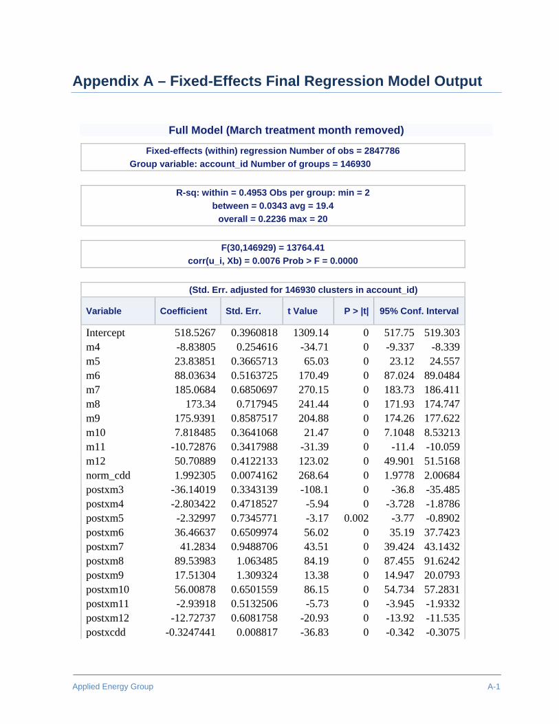
Appendix A – Fixed-Effects Final Regression Model Output
Full Model (March treatment month removed)
Fixed-effects (within) regression Number of obs = 2847786
Group variable: account_id Number of groups = 146930
R-sq: within = 0.4953 Obs per group: min = 2
between = 0.0343 avg = 19.4
overall = 0.2236 max = 20
F(30,146929) = 13764.41
corr(u_i, Xb) = 0.0076 Prob > F = 0.0000
(Std. Err. adjusted for 146930 clusters in account_id)
Variable Coefficient Std. Err. t Value P > |t| 95% Conf. Interval
Intercept 518.5267 0.3960818 1309.14 0 517.75 519.303m4 -8.83805 0.254616 -34.71 0 -9.337 -8.339m5 23.83851 0.3665713 65.03 0 23.12 24.557m6 88.03634 0.5163725 170.49 0 87.024 89.0484m7 185.0684 0.6850697 270.15 0 183.73 186.411m8 173.34 0.717945 241.44 0 171.93 174.747m9 175.9391 0.8587517 204.88 0 174.26 177.622m10 7.818485 0.3641068 21.47 0 7.1048 8.53213m11 -10.72876 0.3417988 -31.39 0 -11.4 -10.059m12 50.70889 0.4122133 123.02 0 49.901 51.5168norm_cdd 1.992305 0.0074162 268.64 0 1.9778 2.00684postxm3 -36.14019 0.3343139 -108.1 0 -36.8 -35.485postxm4 -2.803422 0.4718527 -5.94 0 -3.728 -1.8786postxm5 -2.32997 0.7345771 -3.17 0.002 -3.77 -0.8902postxm6 36.46637 0.6509974 56.02 0 35.19 37.7423postxm7 41.2834 0.9488706 43.51 0 39.424 43.1432postxm8 89.53983 1.063485 84.19 0 87.455 91.6242postxm9 17.51304 1.309324 13.38 0 14.947 20.0793postxm10 56.00878 0.6501559 86.15 0 54.734 57.2831postxm11 -2.93918 0.5132506 -5.73 0 -3.945 -1.9332postxm12 -12.72737 0.6081758 -20.93 0 -13.92 -11.535postxcdd -0.3247441 0.008817 -36.83 0 -0.342 -0.3075

SCE Home Energy Reports Program – Savings Assessment
A-2 Applied Energy Group
postxtrtxm4 -1.873765 0.5983045 -3.13 0.002 -3.046 -0.7011 postxtrtxm5 -4.618361 0.7125964 -6.48 0 -6.015 -3.2217 postxtrtxm6 -6.172819 0.8903766 -6.93 0 -7.918 -4.4277 postxtrtxm7 -7.970365 1.226794 -6.5 0 -10.37 -5.5659 postxtrtxm8 -8.504313 1.345554 -6.32 0 -11.14 -5.8671 postxtrtxm9 -5.824878 1.352367 -4.31 0 -8.475 -3.1743 postxtrtxm10 -6.366926 0.8196778 -7.77 0 -7.973 -4.7604 postxtrtxm11 -4.777219 0.7501779 -6.37 0 -6.248 -3.3069 postxtrtxm12 -5.409894 0.9287761 -5.82 0 -7.23 -3.5895
Related Documents