Scene-Based Nonuniformity Correction for Focal Plane Arrays by the Method of the Inverse Covariance Form

Scene-based nonuniformity correction for focalplane arrays by the method of the inversecovariance form

Sergio N. Torres, Jorge E. Pezoa, and Majeed M. Hayat

What is to our knowledge a new scene-based algorithm for nonuniformity correction in infrared focal-plane array sensors has been developed. The technique is based on the inverse covariance form of theKalman filter �KF�, which has been reported previously and used in estimating the gain and bias of eachdetector in the array from scene data. The gain and the bias of each detector in the focal-plane array areassumed constant within a given sequence of frames, corresponding to a certain time and operationalconditions, but they are allowed to randomly drift from one sequence to another following a discrete-timeGauss–Markov process. The inverse covariance form filter estimates the gain and the bias of eachdetector in the focal-plane array and optimally updates them as they drift in time. The estimation isperformed with considerably higher computational efficiency than the equivalent KF. The ability of thealgorithm in compensating for fixed-pattern noise in infrared imagery and in reducing the computationalcomplexity is demonstrated by use of both simulated and real data. © 2003 Optical Society of America

OCIS codes: 100.2550, 040.1520, 110.3080, 100.3010, 100.3020.

1. Introduction

Focal-plane array �FPA� sensors are frequently usedin a variety of visible and infrared imaging applica-tions.1 It is well known, however, that the perfor-mance of charge-coupled device infrared FPA sensorsis seriously affected by the random spatial variationin the response of the array elements. The spatialnonuniformity in the array output, also referred to asfixed-pattern noise �FPN�, is generally due to �1� theminute detector-to-detector variations in the opto-electronic characteristics of the detectors and �2� fac-tors related to the array’s readout circuitry andarchitecture. FPN is present even in the most ad-vanced mid-wavelength and long-wavelength infra-red sensors, and as one expects, it causes thebroadening of the modulation transfer function andreduces the temperature-resolving capability of ther-

S. N. Torres and J. E. Pezoa are with the Department of Elec-trical Engineering, University of Concepcion, Casilla 160-C, Con-cepcion, Chile. Their e-mail addresses are [email protected] [email protected]. M. M. Hayat is with the Department ofElectrical and Computer Engineering, University of New Mexico,Albuquerque, New Mexico 87131-1356. M. M. Hayat’s e-mail [email protected].

Received 20 January 2003; revised manuscript received 13 June2003.

0003-6935�03�295872-10$15.00�0© 2003 Optical Society of America

5872 APPLIED OPTICS � Vol. 42, No. 29 � 10 October 2003

mal imaging systems.2 Moreover, FPN can compro-mise the effectiveness of multi-sensor systems as itreduces the accuracy of the motion-estimation algo-rithms used by such systems. It is also known thatFPN is not totally stationary but instead it variesslowly in time. Clearly, this drift in FPN makes aone-time laboratory calibration ineffective. Ofcourse, one can calibrate frequently �e.g., by using auniform black-body radiation source as a target�,which would unfortunately require halting normalimaging operation during each calibration process.

In contrast to calibration-based nonuniformity cor-rection �NUC�, scene-based NUC is the process ofFPN compensation by use of the very scenes or ob-jects that are being imaged. However, the nondis-ruptive nature of scene-based NUC comes at theexpense of compromising radiometric accuracy,which may be required in certain applications such asspectral sensing but may be less critical in other ap-plications such as thermal imaging. Scene-basedNUC methods normally employ an image sequenceand rely on motion �or changes in the actual scene� toprovide diversity in the scene temperature per detec-tor. This temperature diversity, in turn, provides astatistical reference point, common to all detectors,according to which the nonuniformity in the detec-tors’ responses can be equalized.

To date, numerous scene-based NUC techniqueshave been reported in the literature.3–13 Our group,

in particular, has been active in the development ofnovel scene-based algorithms for NUC based on sta-tistical estimation theory.14–17 We have lately de-veloped a Gauss–Markov dynamical model to capturethe slow variation in the FPN and utilized the modelto adaptively estimate the nonuniformity in the gainand bias by use of a Kalman filter �KF�.16,17 Theinput to the KF is taken as a sequence of fixed-lengthvectors of readout values representing a block offrames over which no significant drift occurs in thedetectors’ gains and biases. As drift occurs and as anew vector of observations �block of frames� arrives,the KF updates the estimates of the gain and the biasof each detector. In this way, the valuable informa-tion contained in the old estimates is preserved andefficiently used in forming the current state of non-uniformity.

In this paper, we develop what is to our knowledgea new version of our earlier KF–based NUC tech-nique17 that is based on the inverse covariance form�ICF� of the KF. The ICF technique is computation-ally far more efficient than the original KF, especiallywhen the dimension of the measurements is muchgreater than the dimension of the state vector �com-prising the gain and bias�. For example, in the ICFapproach we require the inversion of a diagonal ma-trix with dimensions dictated by the length of theobservation vector �e.g., �100� while in the originalKF,17 the inverse of a non-diagonal matrix of thesame dimension is required. In addition to its su-perior computational efficiency, the ICF technique isbetter suited than its KF–based predecessor for sit-uations where no reliable knowledge of the initialstate of the gain and bias for each detector is avail-able.18

This paper is organized as follows. In Section 2the original KF–based NUC technique is reviewed.The ICF-based NUC technique is developed in Sec-tion 3. In Section 4 the ICF-based NUC technique istested with sequences of infrared data with simu-lated nonuniformity and drift and its equivalence tothe KF–based technique is empirically shown. InSection 5 the technique is applied to six sequences ofreal infrared data. The conclusions of the paper aresummarized in Section 6.

2. Nonuniformity Model and the Kalman Filter

In this paper we adopt the linear-detector responseassumption for which the detector output is approx-imately modeled with a temperature-independentgain and bias.16,17 For a single detector in the FPA,vectors of readout data are considered correspondingto a series of blocks of frames for which no significantdrift in the gain and the bias occurs within eachblock. For the kth block of frames, the linear input–output relation of the ijth detector in the nth frame isapproximated by1,17

Ykij�n� � Ak

ijTkij�n� � Bk

ij � Vkij�n�, (1)

where Akij and Bk

ij are the ijth detector’s gain andbias, respectively, at the kth block of frames. Tk

ij�n�

represents the average number of photons that aredetected by the ijth detector during the integrationtime associated with the nth frame of the kth block.Vk

ij�n� is the additive readout �temporal� noise asso-ciated to the ijth detector for the nth frame during thekth block of frames. In addition, the vector Yk

ij ��Yk

ij�1� Ykij�2� . . . Yk

ij�lk��T is an lk dimensional vectorof readout values for the ijth element of the FPAassociated with the kth block. For simplicity of no-tation, the pixel superscripts ij will be omitted withthe understanding that all operations are performedon a pixel-by-pixel basis.

According to the Gauss–Markov model that we in-troduced in our prior work,17 we model the slow driftin the gain and the bias from one block of frames toanother by

�Ak�1

Bk�1� � ��k 0

0 k��Ak

Bk� � �1 0

0 1��Wk�1�

Wk�2�� , (2)

which we can write compactly as

Xk�1 � �kXk � GkWk. (3)

Here Xk is the state vector comprising the gain Ak andthe bias Bk at the kth block time and k is the 2 � 2transition diagonal matrix between the states at kand k � 1, and its diagonal elements are the param-eters �k and k representing the level of drift in thegain and bias, respectively, between consecutiveblocks. Gk is a 2 � 2 noise identity matrix thatrandomly relates the driving �or process� noise vectorWk to the state vector Xk. The components of Wk areWk

�1� and Wk�2�, the random driving noise for the gain

and the bias, respectively, at the kth block time. Akey requirement that we will impose on Eq. �2� is thatthe state vector must be a stationary random processbecause, in practice, drift in the gain and the biasrandomly changes the FPN but it should not alter itsseverity. All others assumptions are shown and jus-tified in detail elsewhere.17

The observation model for a given block of frames isan extension of the linear model �1� and it can be castas

�Yk�1�

···Yk�lk�

� � �Tk�1� 1

······

Tk�lk� 1�Ak

Bk� � �

Vk�1�···

Vk�lk�� (4)

or

Yk � HkXk � Vk, (5)

where Hk is the observation matrix of dimension lk �2 and Vk is the additive lk-dimensional temporalnoise vector. The main assumption in the observa-tion model �4� is that the input Tk�n� in the kth blockin any detector is an independent sequence ofuniformly-distributed random variables in the range�Tk

min, Tkmax� common to all detectors in each block of

frames.17

The KF–based NUC algorithm developed earlier17

will be briefly visited here for completeness and com-

10 October 2003 � Vol. 42, No. 29 � APPLIED OPTICS 5873

parison with the ICF technique. The algorithm isbased on the following iterations17:

Xk � �k�1Xk�1 � Mk�1T, (6)

Pk � �k�1Pk�1�k�1T � Gk�1Qk�1Gk�1

T, (7)

Kk � PkHkT�HkPkHk

T � Sk��1, (8)

Sk � Rk � Tk

2� A0

2 � A0�Ilk,lk, (9)

Xk � Xk � Kk�Yk � HkXk�, (10)

Pk � �I2,2 � KkHk�Pk, (11)

with the initial conditions

X0 � E�X0� � �A0

B0� , P0 � � � � A0

2 00 B0

2� .

(12)

In the above, Xk� and Xk are respectively the a prioriand the current state estimates, Pk and Pk are re-spectively the a priori and the current error covari-ance matrices, and Kk is the Kalman gain matrix.The quantities Qk and Rk are the auto and crosscovariance functions of the driving noise and the ad-ditive noise, respectively, Hk is the mean of the ob-servation matrix, Mk is a vector containing the meanof the driver noise,16,17 Tk

2 is the variance of theinput infrared signal, and finally, A0 �B0� and A0

2

� B0

2� are the mean and variance of the initial condi-tion for the gain �bias�, respectively. The symbolsI2,2 and Ilk,lk

represent identity matrices of designateddimensions. Note that the matrices Rk and Sk arediagonal, square, and lk dimensional. Also, notethat Eqs. �6� and �7� are the KF updates, Eq. �8� yieldsthe Kalman gain, and Eqs. �10� and �11� are the mea-surement updates.17

The foregoing Gauss–Markov model for the gain andbias is stable �i.e., it has bounded moments� since thedrift parameters �k and k are taken to be strictly lessthan unity. Moreover, the estimation algorithm isalso stable in that the error covariance matrix is con-vergent.18,19 In our prior work, the convergence of theKF was tested with simulated data by showing thatthe error covariance matrix Pk converges to a deter-ministic matrix.17,20 Finally, according to our experi-ence, we have never observed any instabilities whenapplying the algorithm to real infrared imagery.

With the above KF at hand, we proceed to developthe ICF of the filter.

3. Inverse Covariance Form of the Kalman Filter

The KF–based technique described in Section 2 nor-mally estimates the nonuniformity parameters byuse of a very large number of readout data. To ac-commodate such large data efficiently, the KF may bereplaced by an equivalent ICF filter, which is an al-ternate form of the filter that produces the same stateestimates but leads to substantial savings in comput-ing operations and also provides improved numericalstability.18 In this paper the ICF is derived follow-

ing the standard procedures given in Minkler andMinkler,18 which consist of three main steps: �1�definition of the new equivalent state variables to beestimated, �2� application of the matrix inversionlemma to the Kalman-filter recursions to obtain thedual relationship for Xk� , Pk� , Kk, Xk, and Pk, and �3�determining the new initial conditions by use of thedefinition given in step 1.

A. Definition of the New Equivalent State Variables

The ICF is an alternative form of the KF for which theinverse of the error covariance matrix, Pk

�1, is prop-agated in each iteration of the filter. Therefore, theICF inherits the convergence properties of its equiv-alent KF. Following Minkler and Minkler,18 thenew equivalent variable to estimate, ak, is defined as

ak – Pk�1Xk, (13)

where ak is transmitted from one iteration of thefilter to another instead of transmitting the errorcovariance matrix Pk� and the estimate Xk.

B. ICF Algorithm

We begin by recasting the first result of the matrixinversion lemma, which states that for any non-singular matrices L, M, and N, �L � MNT��1 � L�1 �L�1M�I � NTL�1M��1NTL�1. We now apply thisresult to Eqs. �7�, �8�, and �11� to obtain expressionsfor �Pk ��1 and Pk

�1 in terms of the system parame-ters Hk, Qk�1, Sk�1, and �k�1.

Next, we invoke the second result of the matrixinversion lemma, which asserts that �L �MNT��1M � L�1M�I � NTL�1M�. Now by applyingthis result and using the definition in �13�, we canrewrite Eqs. �6� and �10� to get a recursive expressionfor ak� and ak in terms of ak�1. With the above cal-culations, the algorithm for the ICF of the KF isobtained and the recursions involved are listed below:

ak� � �I2,2 � Dk�1Gk�1T���k�1

�1ak�1 � Ck�1Mk�1T�,

(14)

�Pk��1 � �I2,2 � Dk�1Gk�1

T�Ck�1, (15)

Ck�1 – �k�1�TPk�1

�1�k�1�1, (16)

Dk�1 – Ck�1Gk�1�Qk�1�1 � Gk�1

TCk�1Gk�1��1, (17)

ak � ak � HkTSk

�1Yk, (18)

Pk�1 � �Pk�

�1 � HkTSk

�1Hk. (19)

Equations �14� and �15� are the time updates of theICF and the measurement update equations aregiven by Eqs. �18� and �19�.

Initial Conditions. The initial conditions for theICF of the filter can be derived by use of the definitionin Eq. �13� as follows. In particular, we have

P0�1 – ��1, (20)

a� 0 – ��1X0. (21)

5874 APPLIED OPTICS � Vol. 42, No. 29 � 10 October 2003

For estimation problems where no a priori knowledgeof the initial system state is available, this algorithmis less susceptible to saturation problems within theequations, and in that sense, the algorithm may pro-vide a numerically more stable approach.18 In par-ticular the ICF can be utilized with the initialcondition P0

�1 � 0, corresponding to an infinite P0.Note that in the traditional KF, this situation leads tosaturation problems that consequently lead to signif-icant �and possibly catastrophic� loss in numericalaccuracy.

C. Comments on Computational Efficiency

We proceed to theoretically compare the number ofoperations per pixel and per block of frames betweenthe ICF and the traditional KF assuming that thetemporal readout noise and that the range of theinput irradiance �Tk

max, Tkmin� are both common to

all detectors on the FPA, but they may vary fromblock to block. Under the above assumptions, foreach iteration k, the KF involves the inversion of thelk � lk matrix �HkPk�Hk

T � Sk��1. However, the ICFinvolves the inversion of the lk dimension diagonalmatrix �Sk��1.

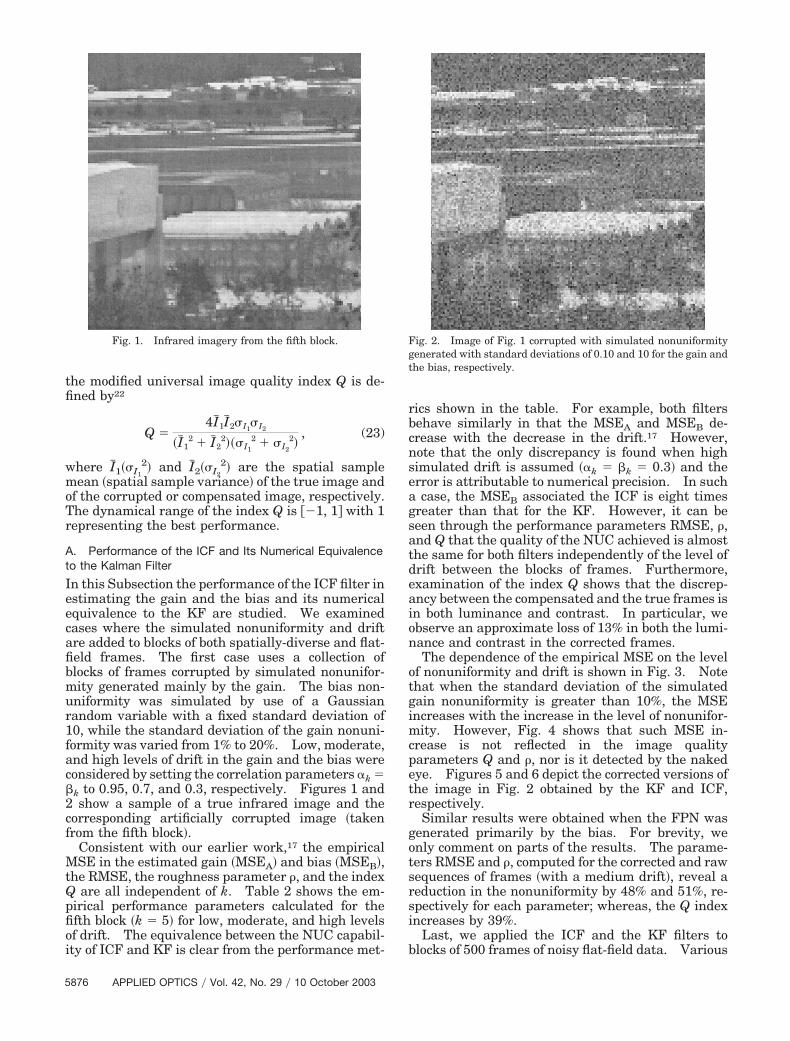
Table 1 shows the number of operations, per pixeland per block of frames at the kth iteration, requiredfor the KF and the ICF. Note that for the KF, therelationship obtained between lk and the number ofoperations is a third-order polynomial, while in thecase of the ICF filter it is a second-order polynomial.Thus, a great reduction in computational load can beachieved. For example, with a block length of 500frames, the KF needs 126,505,038 additions and126,020,040 multiplications, while the ICF calculates1,247,562 additions and 1,004,100 multiplications.Last, note that in Table 1 are detailed the nonstand-ard operations �in the context of a traditional KF witha deterministic observation matrix� that the NUCproblem introduced in both the KF and the ICF fil-ter.17 �These refer to the operations in which thestatistics of the random observation matrix H areinvolved.�

4. Applications to Simulated Infrared Data

In this Section the performance of the ICF filter isstudied and compared with the performance of thetraditional KF16,17 by applying the algorithms to 8-bitinfrared image sequences corrupted by simulatednonuniformity and drift. In all simulations, thegain and the bias are considered as mutually uncor-

related Gaussian random variables with mean valuesof unity and zero, respectively. Different levels ofnonuniformity are introduced by varying the stan-dard deviation of the gain and the bias. Differentlevels of drift in these parameters are also consideredby modifying the inter-block correlation parameters�k and k. Temporal noise is simulated by use of azero-mean Gaussian random variable that is uncor-related to both gain and bias. The standard devia-tion of temporal noise is considered fixed atunity.11,14,15,17,21 One hundred trials of each casewere generated, and each trial included ten blocks,each containing 500 frames. NUC is performed bysubtracting the estimated bias from the readout dataand dividing the outcome by the estimated gain.

The performance of the ICF is evaluated by meansof five metrics. To assess the estimation process, wecompute the mean-square error �MSE� per block byaveraging the square of the differences between thetrue and the estimated gain and bias over the entirearray and all frames within each sequence. NUCcapability is examined in terms of the root-mean-square error �RMSE�, the correctability index, c, andthe roughness parameter, �. The RMSE is definedas the square root of the average �over the entirearray and block of frames� of the square of the differ-ence between the true and the estimated collectedphotons in each pixel. The correctability parameteris computed with simulated flat-field data as thesquare root of the ratio between the FPN and thetemporal readout noise.1,14,21 The roughness pa-rameter � is computed for any image f by use of14

�� f � –h1*f 1 � h2*f 1

f 1, (22)

where h1�i, j� � �i�1, j � �i, j and h2�i, j� � �i, j�1 � �i, j,respectively, �ij is the Kronecker delta, f 1 is the�1-norm of f, and * represents discrete convolution.Note that � is zero for a uniform image, and it in-creases with the pixel-to-pixel variation in the image.Finally, an image-quality index that was recently in-troduced by Wang and Bovik22 is modified and usedhere to further assess NUC capability. The pro-posed index is designed to regard any image distor-tion as a combination of two factors: luminancedistortion and contrast distortion. Mathematically,

Table 1. Number of Operations �per Pixel and per Block of Frames�a

Kalman Filter Inverse Covariance Form

Additions lk2 � 3lk

2p � lk�2p2 � p� � 3p3 � p2�m � 2� �p�m2 � 2m � 1�

lk2�2p � 1� � lk�p2 � p � 1� � 4p3 � p2�4m � 1� �p�2m2 � 3m � 1� � m3

Multiplications lk3 � 2lk

2p � lk�5p2 � 4p� � 3p3 � p2�m � 2�� p�m2 � m�

2lk2p � lk�p2 � p � 2� � 4p3 � p2�4m � 3� � 2pm2

� m3

aNumber that the Kalman filter and the inverse covariance form filter require for the kth iteration. p represents the dimension of thesystem state variables �which is 2 in our case� and lk is the length of the observation vector. m represents the dimension of the randomdriving noise �also 2 in our case�.

10 October 2003 � Vol. 42, No. 29 � APPLIED OPTICS 5875

the modified universal image quality index Q is de-fined by22

Q �4I�1I�2 I1

I2

�I�12 � I�2

2�� I1

2 � I2

2�, (23)

where I�1� I1

2� and I�2� I2

2� are the spatial samplemean �spatial sample variance� of the true image andof the corrupted or compensated image, respectively.The dynamical range of the index Q is ��1, 1� with 1representing the best performance.

A. Performance of the ICF and Its Numerical Equivalenceto the Kalman Filter

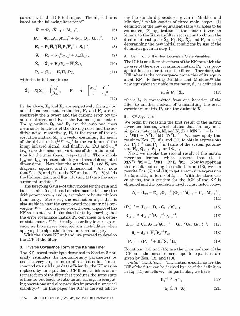
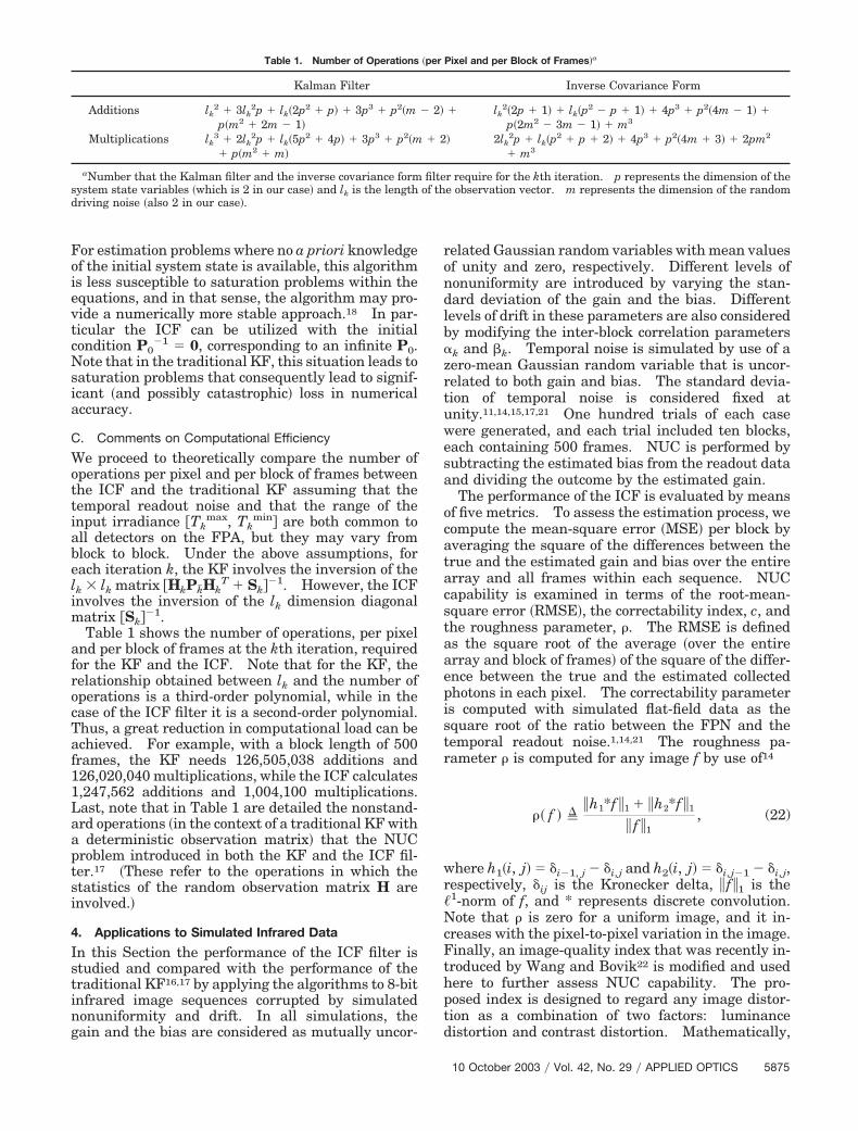
In this Subsection the performance of the ICF filter inestimating the gain and the bias and its numericalequivalence to the KF are studied. We examinedcases where the simulated nonuniformity and driftare added to blocks of both spatially-diverse and flat-field frames. The first case uses a collection ofblocks of frames corrupted by simulated nonunifor-mity generated mainly by the gain. The bias non-uniformity was simulated by use of a Gaussianrandom variable with a fixed standard deviation of10, while the standard deviation of the gain nonuni-formity was varied from 1% to 20%. Low, moderate,and high levels of drift in the gain and the bias wereconsidered by setting the correlation parameters �k �k to 0.95, 0.7, and 0.3, respectively. Figures 1 and2 show a sample of a true infrared image and thecorresponding artificially corrupted image �takenfrom the fifth block�.

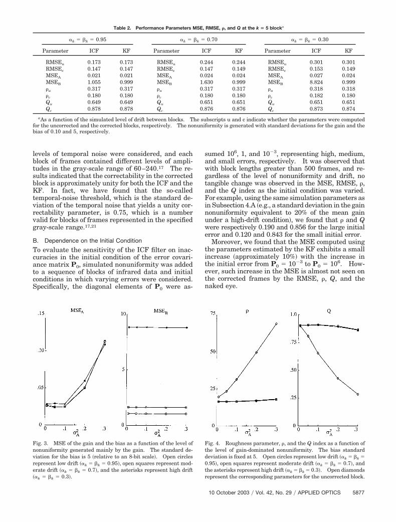
Consistent with our earlier work,17 the empiricalMSE in the estimated gain �MSEA� and bias �MSEB�,the RMSE, the roughness parameter �, and the indexQ are all independent of k. Table 2 shows the em-pirical performance parameters calculated for thefifth block �k � 5� for low, moderate, and high levelsof drift. The equivalence between the NUC capabil-ity of ICF and KF is clear from the performance met-

rics shown in the table. For example, both filtersbehave similarly in that the MSEA and MSEB de-crease with the decrease in the drift.17 However,note that the only discrepancy is found when highsimulated drift is assumed ��k � k � 0.3� and theerror is attributable to numerical precision. In sucha case, the MSEB associated the ICF is eight timesgreater than that for the KF. However, it can beseen through the performance parameters RMSE, �,and Q that the quality of the NUC achieved is almostthe same for both filters independently of the level ofdrift between the blocks of frames. Furthermore,examination of the index Q shows that the discrep-ancy between the compensated and the true frames isin both luminance and contrast. In particular, weobserve an approximate loss of 13% in both the lumi-nance and contrast in the corrected frames.

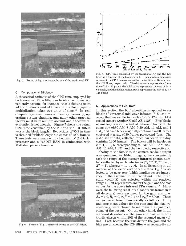
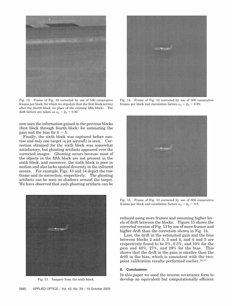
The dependence of the empirical MSE on the levelof nonuniformity and drift is shown in Fig. 3. Notethat when the standard deviation of the simulatedgain nonuniformity is greater than 10%, the MSEincreases with the increase in the level of nonunifor-mity. However, Fig. 4 shows that such MSE in-crease is not reflected in the image qualityparameters Q and �, nor is it detected by the nakedeye. Figures 5 and 6 depict the corrected versions ofthe image in Fig. 2 obtained by the KF and ICF,respectively.

Similar results were obtained when the FPN wasgenerated primarily by the bias. For brevity, weonly comment on parts of the results. The parame-ters RMSE and �, computed for the corrected and rawsequences of frames �with a medium drift�, reveal areduction in the nonuniformity by 48% and 51%, re-spectively for each parameter; whereas, the Q indexincreases by 39%.

Last, we applied the ICF and the KF filters toblocks of 500 frames of noisy flat-field data. Various

Fig. 1. Infrared imagery from the fifth block. Fig. 2. Image of Fig. 1 corrupted with simulated nonuniformitygenerated with standard deviations of 0.10 and 10 for the gain andthe bias, respectively.

5876 APPLIED OPTICS � Vol. 42, No. 29 � 10 October 2003

levels of temporal noise were considered, and eachblock of frames contained different levels of ampli-tudes in the gray-scale range of 60–240.17 The re-sults indicated that the correctability in the correctedblock is approximately unity for both the ICF and theKF. In fact, we have found that the so-calledtemporal-noise threshold, which is the standard de-viation of the temporal noise that yields a unity cor-rectability parameter, is 0.75, which is a numbervalid for blocks of frames represented in the specifiedgray-scale range.17,21

B. Dependence on the Initial Condition

To evaluate the sensitivity of the ICF filter on inac-curacies in the initial condition of the error covari-ance matrix P0, simulated nonuniformity was addedto a sequence of blocks of infrared data and initialconditions in which varying errors were considered.Specifically, the diagonal elements of P0 were as-

sumed 106, 1, and 10�3, representing high, medium,and small errors, respectively. It was observed thatwith block lengths greater than 500 frames, and re-gardless of the level of nonuniformity and drift, notangible change was observed in the MSE, RMSE, �,and the Q index as the initial condition was varied.For example, using the same simulation parameters asin Subsection 4.A �e.g., a standard deviation in the gainnonuniformity equivalent to 20% of the mean gainunder a high-drift condition�, we found that � and Qwere respectively 0.190 and 0.856 for the large initialerror and 0.120 and 0.843 for the small initial error.

Moreover, we found that the MSE computed usingthe parameters estimated by the KF exhibits a smallincrease �approximately 10%� with the increase inthe initial error from P0 � 10�3 to P0 � 106. How-ever, such increase in the MSE is almost not seen onthe corrected frames by the RMSE, �, Q, and thenaked eye.

Fig. 3. MSE of the gain and the bias as a function of the level ofnonuniformity generated mainly by the gain. The standard de-viation for the bias is 5 �relative to an 8-bit scale�. Open circlesrepresent low drift ��k � k � 0.95�, open squares represent mod-erate drift ��k � k � 0.7�, and the asterisks represent high drift��k � k � 0.3�.

Fig. 4. Roughness parameter, �, and the Q index as a function ofthe level of gain-dominated nonuniformity. The bias standarddeviation is fixed at 5. Open circles represent low drift ��k � k �0.95�, open squares represent moderate drift ��k � k � 0.7�, andthe asterisks represent high drift ��k � k � 0.3�. Open diamondsrepresent the corresponding parameters for the uncorrected block.

Table 2. Performance Parameters MSE, RMSE, �, and Q at the k � 5 blocka

�k � k � 0.95 �k � k � 0.70 �k � k � 0.30

Parameter ICF KF Parameter ICF KF Parameter ICF KF

RMSEu 0.173 0.173 RMSEu 0.244 0.244 RMSEu 0.301 0.301RMSEc 0.147 0.147 RMSEc 0.147 0.149 RMSEc 0.153 0.149MSEA 0.021 0.021 MSEA 0.024 0.024 MSEA 0.027 0.024MSEB 1.055 0.999 MSEB 1.630 0.999 MSEB 8.824 0.999�u 0.317 0.317 �u 0.317 0.317 �u 0.318 0.318�c 0.180 0.180 �c 0.180 0.180 �c 0.182 0.180Qu 0.649 0.649 Qu 0.651 0.651 Qu 0.651 0.651Qc 0.878 0.878 Qc 0.876 0.876 Qc 0.873 0.874

aAs a function of the simulated level of drift between blocks. The subscripts u and c indicate whether the parameters were computedfor the uncorrected and the corrected blocks, respectively. The nonuniformity is generated with standard deviations for the gain and thebias of 0.10 and 5, respectively.

10 October 2003 � Vol. 42, No. 29 � APPLIED OPTICS 5877

C. Computational Efficiency

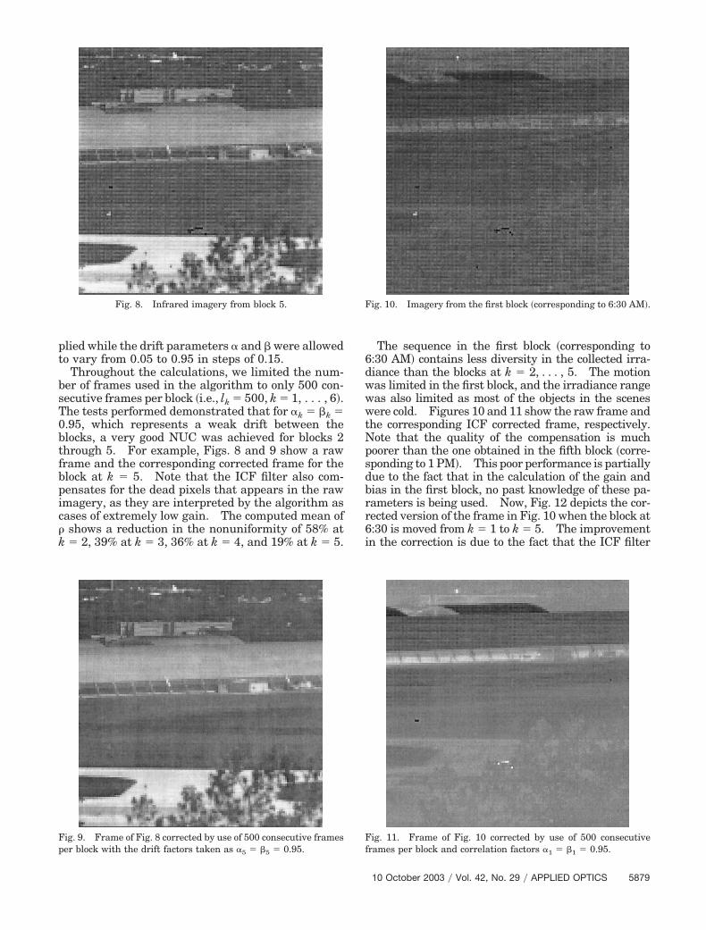
A theoretical estimate of the CPU time employed byboth versions of the filter can be obtained if we con-veniently assume, for instance, that a floating-pointaddition takes a unit of time and the floating-pointmultiplication takes two units of time.23 In realcomputer systems, however, memory hierarchy, op-erating system planning, and many other practicalfactors must be taken into account and a theoreticalevaluation is not enough. Figure 7 shows the actualCPU time consumed by the KF and the ICF filtersversus the block length. Reductions of 55% in timeis obtained for block lengths in excess of 1000 frames.These tests were made with a Pentium IV �1.6 GHz�processor and a 768-MB RAM in conjunction withMatlab’s cputime function.

5. Applications to Real Data

In this section the ICF algorithm is applied to sixblocks of terrestrial mid-wave infrared �3–5 �m� im-agery that were collected with a 128 � 128 InSb FPAcooled camera �Amber Model AE-4128�. Five blocksof imagery were collected at different hours of thesame day �6:30 AM, 8 AM, 9:30 AM, 11 AM, and 1PM�, and each block originally contained 4200 framescaptured at a rate of 30 frames per second �fps�. Thesixth set of data, collected much earlier in the day,contains 1200 frames. The blocks will be labeled ask � 1, . . . , 6, corresponding to 6:30 AM, 8 AM, 9:30AM, 11 AM, 1 PM, and the last block, respectively.

Owing to the fact that the camera readout outputwas quantized to 16-bit integers, we convenientlytook the range of the average infrared photon num-bers collected by each detector as �Tk

min, Tkmax� � �0,

216 � 1�, where k � 1, . . . , 6. In addition, the initialinverse of the error covariance matrix P0

�1 is se-lected to be near zero �which implies severe inaccu-racy in the assumed initial condition�. The initialstate vector X0 was selected within the practicalrange �16-bit representation� for the gain and the biasvalues for the above infrared FPA camera.17 More-over, the following set of initial conditions �common toall detectors� were assumed for the gain and bias:A0 � 1.0, B0 � 0, A0

2 � 0.1 and B0

2 � 5000. Thesevalues were chosen heuristically as follows: Unityand zero mean values for the gain and the bias, re-spectively, were chosen to maintain the dynamicalrange of the output. On the other hand, the initialstandard deviations of the gain and bias were arbi-trarily chosen within 10% of the assumed mean val-ues. Last, because the true drift in the gain and thebias are unknown, the ICF filter was repeatedly ap-

Fig. 5. Frame of Fig. 1 corrected by use of the traditional KF.

Fig. 6. Frame of Fig. 1 corrected by use of the ICF Filter.

Fig. 7. CPU time consumed by the traditional KF and the ICFfilter as a function of the block index k. Open circles and crossesrepresent the CPU time consumed by the traditional Kalman andthe ICF filters, respectively. The dotted curve represents a framesize of 32 � 32 pixels, the solid curve represents the case of 64 �64 pixels, and the dashed-dotted curve represents the case of 128 �128 pixels.

5878 APPLIED OPTICS � Vol. 42, No. 29 � 10 October 2003

plied while the drift parameters � and were allowedto vary from 0.05 to 0.95 in steps of 0.15.

Throughout the calculations, we limited the num-ber of frames used in the algorithm to only 500 con-secutive frames per block �i.e., lk � 500, k � 1, . . . , 6�.The tests performed demonstrated that for �k � k �0.95, which represents a weak drift between theblocks, a very good NUC was achieved for blocks 2through 5. For example, Figs. 8 and 9 show a rawframe and the corresponding corrected frame for theblock at k � 5. Note that the ICF filter also com-pensates for the dead pixels that appears in the rawimagery, as they are interpreted by the algorithm ascases of extremely low gain. The computed mean of� shows a reduction in the nonuniformity of 58% atk � 2, 39% at k � 3, 36% at k � 4, and 19% at k � 5.

The sequence in the first block �corresponding to6:30 AM� contains less diversity in the collected irra-diance than the blocks at k � 2, . . . , 5. The motionwas limited in the first block, and the irradiance rangewas also limited as most of the objects in the sceneswere cold. Figures 10 and 11 show the raw frame andthe corresponding ICF corrected frame, respectively.Note that the quality of the compensation is muchpoorer than the one obtained in the fifth block �corre-sponding to 1 PM�. This poor performance is partiallydue to the fact that in the calculation of the gain andbias in the first block, no past knowledge of these pa-rameters is being used. Now, Fig. 12 depicts the cor-rected version of the frame in Fig. 10 when the block at6:30 is moved from k � 1 to k � 5. The improvementin the correction is due to the fact that the ICF filter

Fig. 8. Infrared imagery from block 5.

Fig. 9. Frame of Fig. 8 corrected by use of 500 consecutive framesper block with the drift factors taken as �5 � 5 � 0.95.

Fig. 10. Imagery from the first block �corresponding to 6:30 AM�.

Fig. 11. Frame of Fig. 10 corrected by use of 500 consecutiveframes per block and correlation factors �1 � 1 � 0.95.

10 October 2003 � Vol. 42, No. 29 � APPLIED OPTICS 5879

now uses the information gained in the previous blocks�first block through fourth block� for estimating thegain and the bias for k � 5.

Finally, the sixth block was captured before sun-rise and only one target �a jet aircraft� is seen. Cor-rection obtained for the sixth block was somewhatsatisfactory, but ghosting artifacts appeared over thecorrected images. Ghosting occurs because most ofthe objects in the fifth block are not present in thesixth block, and moreover, the sixth block is poor inmotion and also lacks spatial diversity in the infraredscenes. For example, Figs. 13 and 14 depict the rawframe and its correction, respectively. The ghostingartifacts can be seen as shadows around the target.We have observed that such ghosting artifacts can be

reduced using more frames and assuming higher lev-els of drift between the blocks. Figure 15 shows thecorrected version of Fig. 13 by use of more frames andhigher drift than the correction shown in Fig. 14.

Last, the drift in the estimated gain and the biasbetween blocks 2 and 3, 3 and 4, and 4 and 5 arerespectively found to be 5%, 0.5%, and 10% for thegain and 40%, 27%, and 29% for the bias. Thisshows that the drift in the gain is smaller than thedrift in the bias, which is consistent with the two-point calibration results performed earlier.16,17

6. Conclusions

In this paper we used the inverse covariance form todevelop an equivalent but computationally efficient

Fig. 12. Frame of Fig. 10 corrected by use of 500 consecutiveframes per block, for which we stipulate that the first block arrivesafter the fourth block �in place of the existing fifth block�. Thedrift factors are taken as �5 � 5 � 0.95.

Fig. 13. Imagery from the sixth block.

Fig. 14. Frame of Fig. 13 corrected by use of 500 consecutiveframes per block and correlation factors �6 � 6 � 0.95.

Fig. 15. Frame of Fig. 13 corrected by use of 800 consecutiveframes per block and correlation factors �6 � 6 � 0.8.

5880 APPLIED OPTICS � Vol. 42, No. 29 � 10 October 2003

version of the previously reported Kalman filter tech-nique for nonuniformity correction in FPAs. More-over, our simulations and real data evaluations havetested practically that the ICF of the KF is bettersuited for problems where no reliable estimate of theinitial condition is available. This feature is in ac-cord with the theoretically expected robustness of theICF to erroneous initial conditions.18 The theoreti-cal evaluation demonstrates that the number offloating-point additions and multiplications per pixeland per block of frames in every iteration is a functionof the block length lk. For the original Kalman filter,the relationship obtained between lk and the numberof operations is a third-order polynomial while in thecase of the inverse covariance form filter it is asecond-order polynomial. Empirical results haveshown that the CPU time consumed by the inversecovariance filter is considerably less than the CPUtime employed by the Kalman filter, and that time isindependent of the frame size. For example, for ablock length of 1000 frames reductions of 45%, 41%,and 50% in the CPU time were obtained for framesizes of 128 � 128, 64 � 64, and 32 � 32 pixels,respectively. The performance of the inverse-covariance-form version of the Kalman filter is dem-onstrated by use of simulated and real infraredimagery showing the ability of the technique in up-dating the estimates of the gain and bias nonunifor-mity as new data arrives. Possible extensions of thetechnique include developing an adaptive method forthe estimation of the drift parameters from blocks ofinfrared scene data.

This work was supported by the Fondo Nacional deCiencia y Tecnologıa of the Chilean Government,project number 1020433, and the National ScienceFoundation. The authors thank Ernest E. Arm-strong �OptiMetrics Inc.� for collecting the data, andthe United States Air Force Research Laboratory,Ohio.

References1. G. C. Holst, CCD Arrays, Cameras and Displays �SPIE Optical

Engineering Press, Bellingham, Wash., 1996�.2. P. Tribolet, P. Chorier, A. Manissadjian, P. Costa, and J. P.

Chatard, “High performance infrared detectors at Sofradir,” inInfrared Detectors and Focal Pane Arrays VI, E. L. Dereniakand R. E. Sampson, eds., Proc. SPIE 4028, 438–456 �2002�.

3. P. M. Narendra and N. A. Foss, “Shutterless fixed patternnoise correction for infrared imaging arrays,” in Technical Is-sues in Focal Plane Development, W. S. Chan and E. Krikorian,eds., Proc. SPIE 282, 44–51 �1981�.

4. P. M. Narendra, “Reference-free nonuniformity compensationfor IR imaging arrays,” in Smart Sensors II, D. F. Barbe, ed.,Proc. SPIE 252, 10–17 �1980�.

5. J. G. Harris, “Continuous-time calibration of VLSI sensors forgain and offset variations,” in Smart Focal Plane Arrays andFocal Plane Array Testing, M. Wigdor and M. A. Massie, eds.,Proc. SPIE 2474, 23–33 �1995�.

6. J. G. Harris and Y.-M. Chiang, “Nonuniformity correction us-

ing constant average statistics constraint: analog and digitalimplementations,” in Infrared Technology and ApplicationsXXIII, B. F. Andersen and M. Strojnik, eds., Proc. SPIE 3061,895–905 �1997�.

7. J. G. Harris and Y-M Chiang, “Minimizing the ‘ghosting’ arti-fact in scene-based nonuniformity correction,” in Infrared Im-aging Systems: Design, Analysis, Modeling, and Testing IX,G. C. Holst, ed., Proc. SPIE 3377, 106–113 �1998�.

8. J. G. Harris and Y-M Chiang, “Nonuniformity correction ofinfrared image sequences using the constant-statistics con-straint,” IEEE Trans. Image Process. 8, 1148–1151 �1999�.

9. Y.-M. Chiang and J. G. Harris, “An analog integrated circuitfor continuous-time gain and offset calibration of sensor ar-rays,” J. Analog Int. Circuits Signal Process. 12, 231–238�1997�.

10. W. F. O’Neil, “Experimental verification of dithered scan non-uniformity correction,” in Proceedings of the 1996 Interna-tional Meeting of the Infrared Information SymposiumSpecialty Group on Passive Sensors �Infrared InformationAnalysis Center, Ann Arbor, Michigan, 1997�, Vol. 1, pp. 329–339.

11. R. C. Hardie, M. M. Hayat, E. E. Armstrong, and B. Yasuda,“Scene based nonuniformity correction using video sequencesand registration,” Appl. Opt. 39, 1241–1250 �2000�.

12. B. M. Ratliff, M. M. Hayat, and R. C. Hardie, “An algebraicalgorithm for nonuniformity correction in focal-pane arrays,”J. Opt. Soc. Am. A 19, 1737–1747 �2002�.

13. K. C. Hepfer, S. R. Horman, and B. Horsch, “Method anddevice for improved IR detection with compensations for indi-vidual detector response,” U.S. patent 5,276,319 �4 January1994�.

14. M. M. Hayat, S. Torres, E. E. Armstrong, B. Yasuda, and S. C.Cain, “Statistical algorithm for non-uniformity correction infocal plane arrays,” Appl. Opt. 38, 772–780 �1999�.

15. E. E. Armstrong, M. M. Hayat, R. C. Hardie, S. N. Torres, andB. Yasuda, “Nonuniformity correction for improved registra-tion and high resolution image reconstruction in IR imagery,”in Applications of Digital Image Processing XXII, A. G. Te-scher, ed., Proc. SPIE 3808, 150–161 �1999�.

16. S. N. Torres, M. M. Hayat, E. E. Armstrong, and B. Yasuda, “AKalman-filtering approach for nonuniformity correction infocal-plane array sensors,” in Infrared Imaging Systems: De-sign, Analysis, Modeling, and Testing XI, G. C. Hulst, ed., Proc.SPIE 4030, 196–205 �2000�.

17. S. N. Torres and M. M. Hayat, “Kalman filtering for adaptivenonuniformity correction in infrared focal plane arrays,” J.Opt. Soc. Am. A 20, 470–480 �2003�.

18. G. Minkler and J. Minkler, Theory and Applications of KalmanFiltering �Magellan, Palm Bay, Fla., 1993�.

19. C. Therrien, Discrete Random Signals and Statistical SignalProcessing �Prentice-Hall, Englewood Cliffs, N.J., 1992�.

20. S. N. Torres, “A Kalman filtering approach for non-uniformitycorrection in infrared focal plane array sensors,” Ph.D. disser-tation �University of Dayton, Ohio, 2001�.

21. M. Schultz and L. Caldwell, “Nonuniformity correction andcorrectability of infrared focal plane arrays,” in Infrared Im-aging Systems: Design, Analysis, Modeling, and Testing VI,G. C. Hulst, ed. Proc. SPIE 2470, 200–211 �1995�.

22. Z. Wang and A. Bovik, “A universal image quality index,”IEEE Signal Process. Lett. 9, 81–84 �2002�.

23. J. L. Hennessy and D. A. Patterson, Computer Organizationand Design: The Hardware�Software Interface �MorganKaufmann, Los Altos, Calif., 1997�.

10 October 2003 � Vol. 42, No. 29 � APPLIED OPTICS 5881