Scenario generation of aggregated Wind, Photovoltaics and ...

HAL Id: hal-02081282https://hal.archives-ouvertes.fr/hal-02081282

Submitted on 27 Mar 2019

HAL is a multi-disciplinary open accessarchive for the deposit and dissemination of sci-entific research documents, whether they are pub-lished or not. The documents may come fromteaching and research institutions in France orabroad, or from public or private research centers.

L’archive ouverte pluridisciplinaire HAL, estdestinée au dépôt et à la diffusion de documentsscientifiques de niveau recherche, publiés ou non,émanant des établissements d’enseignement et derecherche français ou étrangers, des laboratoirespublics ou privés.

Scenario generation of aggregated Wind, Photovoltaicsand small Hydro production for power systems

applicationsSimon Camal, Fei Teng, Andrea Michiorri, Georges Kariniotakis, L Badesa

To cite this version:Simon Camal, Fei Teng, Andrea Michiorri, Georges Kariniotakis, L Badesa. Scenario generation ofaggregated Wind, Photovoltaics and small Hydro production for power systems applications. AppliedEnergy, Elsevier, 2019, Volume 242, pp.1396-1406. 10.1016/j.apenergy.2019.03.112. hal-02081282

Scenario generation of aggregated Wind, Photovoltaics and small Hydro productionfor power systems applications

S. Camala, F. Tengb, A. Michiorria, G.Kariniotakisa, L. Badesab

aMINES ParisTech - PSL University, Research Center PERSEE, Sophia Antipolis, FrancebImperial College London, Electrical and Electronic Engineering Department, London, SW7 2AZ, UK

Abstract

This paper proposes a methodology for an efficient generation of correlated scenarios of Wind, Photovoltaics (PV) andsmall Hydro production considering the power system application at hand. The merits of scenarios obtained from adirect probabilistic forecast of the aggregated production are compared with those of scenarios arising from separateproduction forecasts for each energy source, the correlations of which are modeled in a later stage with a multivariatecopula. It is found that scenarios generated from separate forecasts reproduce globally better the variability of amulti-source aggregated production. Aggregating renewable power plants can potentially mitigate their uncertaintyand improve their reliability when they offer regulation services. In this context, the first application of scenariosconsists in devising an optimal day-ahead reserve bid made by a Wind-PV-Hydro Virtual Power Plant (VPP). Scenariosare fed into a two-stage stochastic optimization model, with chance-constraints to minimize the probability of failingto deploy reserve in real-time. Results of a case study show that scenarios generated by separately forecasting theproduction of each energy source leads to a higher Conditional Value at Risk than scenarios from direct aggregatedforecasting. The alternative forecasting methods can also significantly affect the scheduling of future power systemswith high penetration of weather-dependent renewable plants. The generated scenarios have a second application hereas the inputs of a two-stage stochastic unit commitment model. The case study demonstrates that the direct forecast ofaggregated production can effectively reduce the system operational cost, mainly through better covering the extremecases. The comprehensive application-based assessment of scenario generation methodologies in this paper informs thedecision-makers on the optimal way to generate short-term scenarios of aggregated RES production according to theirrisk aversion and to the contribution of each source in the aggregation.

Keywords: Ancillary Services, Chance-constrained Optimization, Forecasting, Renewable Energy, Scenarios,Stochastic Scheduling

1. Nomenclature

1.1. Indicesagg Level of aggregation in the VPPs Index of energy source type in the VPPda Day-ahead variableg Index of thermal generatorsrt Real-time variable↑, ↓ Upward,downward regulationω Index of production scenarios

IThis paper was submitted for review on 03.07.2018. The re-search was carried as part of the European project REstable (Ref-erence Number 77872), supported by the ERA-NET Smart GridsPlus program with financial contribution from the European Com-mission, ADEME, Juelich Research Center, Fundacao para a Cienciae a Tecnologia

Email address: [email protected] (S. Camal)

1.2. Setsc Coefficients of the objective functionG Set of thermal generatorsO Subset of slow thermal generatorsπ Prices for energy and reserve

1.3. VariablesaR Reserve activation probabilityb Binary variable for ramp functionB Vector of decision variables for biddingδ gradient indicator function for Brier Score∆R↑,− Deficit of upward reserve in real-time∆R↓,− Deficit of downward reserve in real-timeEda Energy on the day-ahead marketErt,+ Energy surplus on the real-time marketErt,− Energy deficit on the real-time market

l

l

F Cumulative distribution functionm Marginal distribution function of a copulaoT Objective function for risk-neutral biddingoβ,T Objective function for risk-averse biddingψ Positive variable for ramp functionPLS Load-sheddingP g Power produced by generator gPRC RES curtailmentRda Reserve on the day-ahead marketRrt Reserve on the real-time marketΣ Covariance matrix of Normal variablesu Vector of uniform i.i.d. variablesU Generalized cumulative distribution functionX Vector of features for production forecastingY agg Power production at aggregation level aggyg Binary variable, commitment decision

for generator gzg Startup state of generator g

1.4. Parameters

β Aversion to risk on revenuecLS Load-shedding costcgm Marginal cost of generator gcgnl No-load cost of generator gcgst Startup cost of generator gε Confidence parameter of chance constraintsk Horizon of forecastΩ Number of scenariospω Probability of occurrence for scenario ωPgmax Rated power of unit gPgmsg Minimum stable generation of unit gPgrd Maximum ramp-down capability of unit gPgru Maximum ramp-up capability of unit g

PDω,t Demand in scenario ω and time-step t

PRω,t Power produced by RES in scenario ω

and time-step tt Runtime of forecastτt Duration of time-step t in the two-stage SUCT Period of bidding optimization

2. Introduction

Weather-dependent Renewable Energy Sources (RES)constitute an increasing share of power generation, but theuncertainty of their production raises challenges for theirinteraction with power systems. In particular, the vari-ability of aggregated RES power production must be ac-counted for in power system applications which exploit thecomplementarity between RES (e.g. bidding on electricitymarkets by an aggregator operating RES plants), or con-sider the systemic impact of aggregated RES plants (e.g.scheduling of power systems with high RES penetration).

The complementarity between RES is a subject of in-terest in applications related to the provision of AncillaryServices (AS). Historically, only conventional dispatchablepower plants provided AS, but recent studies have shown

that RES plants of various sources have the technical ca-pacity to offer AS, namely Wind [1], run-of-river hydro [2],and Photovoltaics (PV) [3]. However the uncertainty as-sociated with the production of a single RES plant is toolarge to provide AS with the high level of reliability re-quired by system operators. A first solution to increase thereliability of AS delivered by RES is to combine RES plantswith Energy Storage Systems (ESS) which can compensateforecast error, but with a high investment cost in the caseof static storage [4]. A second solution is to aggregate RESplants blending energy sources and weather conditions, inorder to reduce the uncertainty of the total production[5]. The aggregated plants are coordinated via a VirtualPower Plant (VPP) which ensures sufficient regulation ca-pacity to comply with the stringent pre-qualification testsfor the provision of AS [6]. Such a VPP can integrate otheragents like flexible consumers or ESS from static storagesand electric mobility [7],[8], [9]. Following the ongoingdevelopment of short-term markets for AS [10], method-ologies for the optimal offer of energy and reserve havebeen proposed for wind farms [11],[12], microgrids [13],and aggregated flexible loads [14] [15]. The optimizationmodels of these methodologies rely on probabilistic fore-casts or trajectories of RES production. Adding chanceconstraints to the optimization makes it possible to bal-ance revenue with the technical risk of not supplying re-serve [14]. The realization of these constraints dependson scenarios of RES production, reproducing the expecteduncertainty at short-term. In contrast with the reviewedworks, which considered single energy sources or severalsources independently, the present paper investigates howto forecast the expected interaction between multiple RESat short-term and quantify the associated impact on ASbidding.

The aggregated production of weather-dependent re-newable power plants plays also a major role in the schedul-ing of electrical networks. When scheduling electrical sys-tems, operators decide the commitment decision of gener-ators to meet the demand with minimal cost. At present,AS are scheduled following deterministic rules that involveimposing pre-defined requirements to tackle the uncertain-ties associated with forecasting error and equipment out-ages. As the uncertainty introduced by the total gen-eration of weather-dependent renewable power plants ismuch more significant than that of demand, schedulingprocesses performed under deterministic rules become in-efficient [16] [17] [18] [19]. In contrast, stochastic unit com-mitment models employ scenarios to model the uncertaintyof weather-dependent renewables [20] [21]. These modelsensure economic efficiency and network security.

In both applications introduced above, short-term de-cisions are derived from a stochastic optimization whichrelies on scenarios of aggregated RES production as in-puts. It is known that the quality of the scenarios hasa direct impact on the performance of the optimizationmodel [21]. In the case of short-term horizons, scenar-ios should combine two properties: reproduce the interde-

2

pendence in the aggregated renewable production process,and vary as a function of the influence of explanatory vari-ables such as weather forecasts. The interdependence inRES production comprises classically the temporal depen-dencies between successive lead-times, which is generallynot captured by production forecasts [22], and the possi-ble correlation between power plants. A specific challengefor scenarios of a multi-source RES aggregation is to modelthe dependencies between energy sources, for simultaneousand successive lead-times, while preserving the conditionalresponse to explanatory variables.

A popular method to generate scenarios is to build amultivariate Gaussian copula from probabilistic forecastsof the marginal distributions (e.g. production of a givenwind farm at different lead times [22], or production ofseveral PV plants at different lead times [23]). Copulasare flexible tools to model dependencies in uncertainties,although in problems focused on extreme regions of themarginal distributions, analytical models using exponen-tial functions may be more appropriate [22]. Vine copulas,which form flexible trees of bivariate copulas, have beensuccessfully used for the probabilistic forecast of multi-ple Wind [24] and PV [25] plants. However to the au-thors’ knowledge, neither Gaussian copulas nor Vine cop-ulas have been reported in the literature in the contextof scenarios for a multi-source RES aggregation. Hierar-chical copula models, which base on independent forecastsof each contributor of an aggregation at several hierarchi-cal levels, have been proposed in the context of electricitydemand [? ] and insurance exposure [26]. While these ap-proaches are effective on aggregations which follow natu-rally a tree structure such as electricity networks, their ap-plication on a multi-source RES aggregation which has noobvious hierarchical structure would require a large num-ber of permutations to assess all possible sums betweenplants or sources.

Alternative methods to generate scenarios exist. Timeseries analysis can derive spatio-temporal models for re-newable power plants at multiple sites [27]. The machinelearning approach of [28] builds an iterative neural networkthat outputs scenarios by random generation of errors andstep-ahead forecasts. For stochastic scheduling of powersystems with high penetration by wind power, [20] developa multi-stage scenario tree based on the distribution ofwind forecasting errors. In [21], scenarios of wind forecast-ing errors are generated by a Levy α-stable distribution.These approaches are based on deterministic forecasts ofproduction, which is valid for a single energy source butwould miss important interdependences of uncertainty be-tween energy sources. The Generative Adversarial Net-works of [29] produce trajectories with adequate diversityand similar statistical properties to historical data thanksto the ability of this unsupervised deep learning to learncomplex non-linearities and classify large inputs. The min-imization of the Wasserstein distance between the genera-tor and discriminator provides good climatological proper-ties of the scenarios, and could be applied to multi-source

RES aggregations. However, the solution of [29] proposesonly a classification of typical conditions (e.g. scenariosfor a sunny winter day). This is suitable for long-termscenarios but not directly applicable for short-term scenar-ios where scenarios should reflect the expected conditionssuch as weather forecasts.

In the presented literature few efforts have been madeto assess how different scenario generation approaches im-pact the results of the optimization. More specifically,the use of aggregated, multi-source RES trajectories instochastic optimization has not been frequently investi-gated. Uncertainty in production is of particular interestwhen aggregating power plants of different energy sources,possibly subject to different climates. The present pa-per addresses the challenge of generating scenarios of theoutput of a mix of power plants harvesting different en-ergy sources. The dimension of the forecasting problemis significantly more complex than forecasting single en-ergy sources. Furthermore, we investigate which scenariogeneration method is most suitable considering the frame-work of the applications, with examples for AS biddingand power system scheduling.

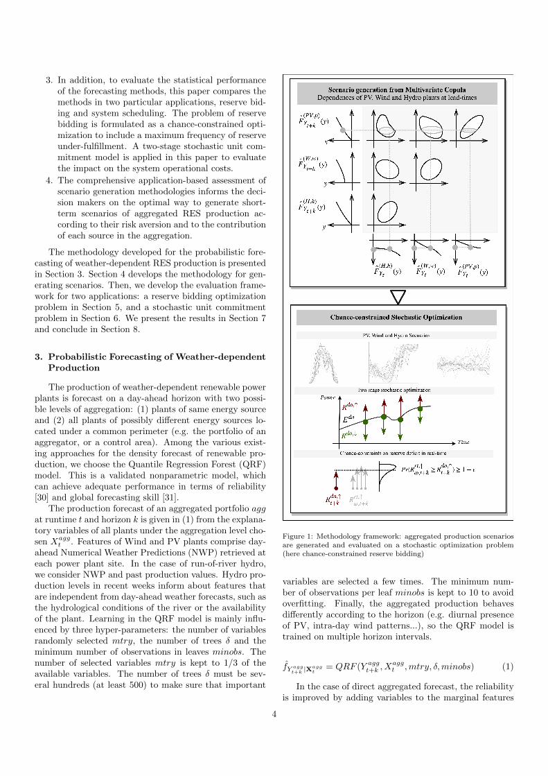
The framework of the paper, illustrated in Figure 1, isstructured as follows: we start by forecasting the produc-tion of a portfolio of PV, Wind and small Hydro plants,separately for each source and directly at the aggregatedlevel. From these probabilistic forecasts we generate sce-narios by applying multivariate copulae on the availablemarginal distributions over the range of lead-times, andover the range of sources in the case of separate forecasts.The Gaussian copula is first applied as a standard spatio-temporal dependence model, and a Vine copula is pro-posed to model the dependencies between separate fore-casts with more flexibility. Then, these scenarios are ap-plied to two relevant case studies, in which the solutionof the stochastic optimization is highly dependent on thecharacterization of the uncertainty. The first case study isthe day-ahead bidding of energy and automatic FrequencyRestoration Reserve (aFRR) by a renewable VPP usinga two-stage stochastic optimization. In the second casestudy, we schedule a network with significant penetrationof Wind, PV and small hydro.

The key contributions of this work are identified asfollows:

1. Firstly, this paper addresses the problem of generat-ing probabilistic forecasts for the aggregated powerof a set of renewable power plants harvesting dif-ferent energy sources. Despite abundant works inthe literature on models that separately forecast PV,Wind or Hydro, the problem has not been tackledjointly.

2. Based on probabilistic forecasts of either the indi-vidual energy sources or the aggregation, this paperproposes to generate scenarios of the aggregated pro-duction, with a multivariate Gaussian copula takinginto account correlations.

3

3. In addition, to evaluate the statistical performanceof the forecasting methods, this paper compares themethods in two particular applications, reserve bid-ing and system scheduling. The problem of reservebidding is formulated as a chance-constrained opti-mization to include a maximum frequency of reserveunder-fulfillment. A two-stage stochastic unit com-mitment model is applied in this paper to evaluatethe impact on the system operational costs.

4. The comprehensive application-based assessment ofscenario generation methodologies informs the deci-sion makers on the optimal way to generate short-term scenarios of aggregated RES production ac-cording to their risk aversion and to the contributionof each source in the aggregation.

The methodology developed for the probabilistic fore-casting of weather-dependent RES production is presentedin Section 3. Section 4 develops the methodology for gen-erating scenarios. Then, we develop the evaluation frame-work for two applications: a reserve bidding optimizationproblem in Section 5, and a stochastic unit commitmentproblem in Section 6. We present the results in Section 7and conclude in Section 8.

3. Probabilistic Forecasting of Weather-dependentProduction

The production of weather-dependent renewable powerplants is forecast on a day-ahead horizon with two possi-ble levels of aggregation: (1) plants of same energy sourceand (2) all plants of possibly different energy sources lo-cated under a common perimeter (e.g. the portfolio of anaggregator, or a control area). Among the various exist-ing approaches for the density forecast of renewable pro-duction, we choose the Quantile Regression Forest (QRF)model. This is a validated nonparametric model, whichcan achieve adequate performance in terms of reliability[30] and global forecasting skill [31].

The production forecast of an aggregated portfolio aggat runtime t and horizon k is given in (1) from the explana-tory variables of all plants under the aggregation level cho-sen Xagg

t . Features of Wind and PV plants comprise day-ahead Numerical Weather Predictions (NWP) retrieved ateach power plant site. In the case of run-of-river hydro,we consider NWP and past production values. Hydro pro-duction levels in recent weeks inform about features thatare independent from day-ahead weather forecasts, such asthe hydrological conditions of the river or the availabilityof the plant. Learning in the QRF model is mainly influ-enced by three hyper-parameters: the number of variablesrandomly selected mtry, the number of trees δ and theminimum number of observations in leaves minobs. Thenumber of selected variables mtry is kept to 1/3 of theavailable variables. The number of trees δ must be sev-eral hundreds (at least 500) to make sure that important

Figure 1: Methodology framework: aggregated production scenariosare generated and evaluated on a stochastic optimization problem(here chance-constrained reserve bidding)

variables are selected a few times. The minimum num-ber of observations per leaf minobs is kept to 10 to avoidoverfitting. Finally, the aggregated production behavesdifferently according to the horizon (e.g. diurnal presenceof PV, intra-day wind patterns...), so the QRF model istrained on multiple horizon intervals.

fY aggt+k |X

aggt

= QRF (Y aggt+k , Xaggt ,mtry, δ,minobs) (1)

In the case of direct aggregated forecast, the reliabilityis improved by adding variables to the marginal features

4

corresponding to each plant of the aggregation: (1) mini-mum and maximum values of variables across plants shar-ing the same source (e.g. minimum and maximum windspeed) help the QRF model explore more robustly the vari-ance of the aggregated production process, (2) lagged val-ues of marginal features add information on the weatherpatterns around the time of prediction or on persistent be-haviour of production for a given energy source. In the caseof separate forecasting by energy source, a preprocessingtreatment of the production variable Y aggt+k helps reduce theimpact of deterministic trends on learning and obtain con-ditional variances independent of conditional means [22].The treatment is specific to each energy source and is car-ried out before summing up the power production data: forWind we apply the logit transform [22], while for PV wenormalize production with a simple analytical model forthe top of atmosphere global horizontal irradiance. Thelogit transform could also been applied to Hydro (by anal-ogy with Wind as a double-bounded production that isnon-linearly dependent on an inflow). However, in thiscase the hydro production is not explained by a waterflow forecast but rather by features mixing production andweather variables, meaning there is no homogeneity in thenon-linear relationships between features and production,and therefore logit transform is not employed.

At the end of this first step of the methodology, weobtain at runtime t, two sets of forecasts for all horizonsk ∈ [1,K] :

1. The total aggregated production for all plants, FY totalt+k

;

2. The production of plants sharing the same energysource, namely Wind, PV and run-of-river Hydro,FYWind

t+k, FY PV

t+k, FY Hydro

t+k.

4. Generation of Production Scenarios

The probabilistic forecasts obtained in the previoussection inform us about the predicted levels of produc-tion and their relative uncertainty. However simple MonteCarlo sampling on the predictive densities obtained doesnot consider correlations resulting thus in non realistic al-ternative forecast scenarios with close horizons or spatialcorrelations between plants or energy sources. In contrast,adding a model of the correlations between the predictivedensities, such as a multivariate copula [? ], produces sce-narios with more realistic behavior with respect to the realproduction patterns.

4.1. Multivariate Copula based on Probabilistic Forecasts

The multivariate copula is a multivariate distributionfunction, the marginals of which should be distributed uni-formly in the rank domain [23]. The marginals are predic-tive densities of the production for specific dimensions ofthe problem, for instance the various horizons or the differ-ent energy sources of the aggregation. Due to the bound-edness of intermittent production, the forecasted distribu-tion function FY of an intermittent production Y is not

strictly monotonous, hence a given power observation yobscan be associated with several quantile values FY (yobs),for instance if yobs is a wind power observation occurringat wind speeds over the nominal speed value. In order toobtain marginals uniformly distributed from intermittentproduction forecasts, we apply to each forecast the distri-butional transform developed by Ruschendorf [32], whichgeneralizes in (2) the property of uniform distribution todiscontinuous Cumulative Distribution Functions (CDFs).

U(y) = FY −(y) + V (FY (y)− FY −(y)) (2)

where V is a random variable following the uniform dis-tribution and FY − is the left-hand CDF of the productionvariable Y . Note that U(y) = FY (y) if the CDF is contin-uous. We can now construct our multivariate copula fromthe transformed marginal distributions.

At this point, we propose two distinct methods. Thefirst method, entitled ”Direct Gaussian” (DG), constructsa multivariate temporal dependence model between thevariables Y totalk , which represent the values taken by thetotal aggregated production at the successive horizons k ∈[1,K]. We start by collecting a series of observed aggre-gated productions ytotalt+k , not included in the training setof the forecasting model, for all horizons k. The positionof these observed productions in the forecast distributionFY total

t+kat each horizon k is evaluated according to (2), and

constitutes a realization utotalt+k of the uniformly distributed

marginal U totalk .

utotalt+k = U totalk (ytotalt+k ), ∀t, ∀k (3)

All marginals are then converted in (4) into normally dis-tributed variables Ztotalk using the probit function Φ [22],forming a multivariate variable Ztotal normally distributedwith a zero mean vector and covariance Σtotal of dimensionK ×K .

ztotalt+k = Ztotalk (ytotalt+k ) = Φ(utotalt+k ), ∀t, ∀k (4)

Ztotal = (Ztotal1 , Ztotal2 , ..., Ztotalk , ..., ZtotalK ) (5)

Ztotal ∼MVN (0,Σtotal) (6)

The density of Ztotal forms a Gaussian copula parametrizedby the mean vector and the covariance matrix, which iscomputed here as the empirical covariance matrix on theobserved normally transformed marginals. A final stepconsists in drawing samples from the copula to generatetrajectories which reproduce the temporal correlation be-tween horizons. To generate Ω distinct scenarios of to-tal aggregated production for a given period of interest[t+ 1, t+K] we:

1. Draw Ω i.i.d.random vectors sω following the uni-form distribution U(0, 1)K , where ω ∈ [1,Ω];

2. Convert them into realizations ztotalω of Ztotal;

3. Generate trajectories ytotal,DGω,t+k for the period of in-terest by applying in (7) the quantile values given byeach zω to the marginal forecasts FY total

t+k:

5

ytotal,DGω,t+k = F−1Y totalt+k

(ztotalω,t+k) ∀ω,∀t, ∀k (7)

A second method is based on the separate forecastingby energy source instead of the direct forecasting of thetotal aggregated production. This approach, entitled ”In-direct Gaussian” (IG), models the dependencies betweenproductions of the different energy sources, over all hori-zons. The observed productions are now collected andaggregated for each energy source separately, resulting inan observation vector ysourcest+k of dimension S, S being thenumber of sources (in the present case S=3 with Wind, PVand small Hydro). The multivariate copula of the variableZsources is constructed in the same way as for the DGmethod, giving a covariance matrix Σsources of dimensionSK×SK. Scenarios are generated by sampling the covari-ance matrix and affecting the resulting quantiles zsourcesω

of dimension SK to the probabilistic forecasts of the re-spective energy sources for the period of interest. Lastlythe obtained equiprobable trajectories are summed acrossall sources in (8) to form Ω trajectories of total aggregatedproduction.

ytotal,IGω,t+k =∑

s=[1,S]

F−1Y st+k

(zsources,sω,t+k ) ∀ω ∈ [1,Ω],∀t,∀k (8)

A variant of this method, entitled ”Indirect Vine” (IV),consists in replacing the Gaussian copula by a regular Vinecopula to model non-Gaussian dependencies between hori-zons and energy sources. A regular Vine copula is formedsequentially by joining bivariate copulas into trees. Theselected tree among all possible combinations is the treethat maximizes the sum of empirical rank correlations overthe possible pairs (Maximum Spanning Tree algorithm, see[24]). To generate a number of scenarios Ω from the Vinecopula at horizon t+k (omitted in notations below for thesake of simplicity) we:

1. Draw Ω i.i.d random vectors sω following the uniformdistribution U(0, 1)SK

2. Retrieve the uniform marginal CDF value mω,d, d ∈SK of the production variable Yd, conditioned bythe other variables, by inverting the h-function ofthe Vine copula [24]

mω,d = F−1d|d−1,...,1(sω,d|mω,d−1, ...,mω,1) (9)

3. Invert the CDF of the marginal production variable

F(d)Y to obtain the production trajectory.

yω,d = F−1Y d (zω,d) (10)

In the next section, we evaluate the quality of the trajec-tories of total aggregated production obtained by directaggregated forecasting and separate forecasting by energysource.

4.2. Evaluation of Trajectories

The generated trajectories must reproduce correlationsbetween horizons, locations and energy sources. We assess

the quality of trajectories by a proper score, the Variogram-based score (VS) [33], to determine whether trajectoriesreproduce correctly the main moments of the original pro-duction [23]. The VS of order γ can be expressed in (11) asthe quadratic difference between the Variogram of the orig-inal production data y and the Variogram of the forecasttrajectories yωt. The latter is approximated by the meanof the score over the scenarios. Here, pairs of points areequally weighted, wij = 1. Points with a low correlationand thus a low signal-to-noise ratio are therefore not pe-nalized [33]. The discrimination ability of the score couldbe lower than with a correlation model fitted on data, butwe choose to use equal weights to investigate the wholerange of correlations including long intervals (productiongradients over several hours are an important input forreserve bidding).

V S(γ)t =

∑i,j∈M

wij(|yt,i − yt,j |γ−

1

Ω

∑ω∈[1,Ω]

(|yωt,i − yωt,j |γ))2 (11)

Beyond similarity in the trajectory distributions, tra-jectories should also exhibit characteristic events of theoriginal time series, such as gradients. Gradients up to afew hours are of particular interest when offering reservecapacities: the validity period (contracted duration of ca-pacity) of secondary reserve (aFRR) goes from 15 min inthe Netherlands to 1h in Portugal and 4h in Germany [34].We evaluate the similarity of gradients observed in theoriginal time series with gradients in scenarios by means ofa Brier Score (BS) defined in (13). The events consideredin the score are production gradients δt over an interval∆t, which are higher than a threshold value r, taken asthe average observed gradient over the interval.

δt(y; ∆t) = 1(|yt+∆t − yt| ≥ r) (12)

BS =1

T

T∑t=1

(1

Ω

∑ω∈[1,Ω]

δt(yω; ∆t)− δt(y; ∆t))2 (13)

The generated scenarios are now applied to two stochas-tic optimization problems, reserve bidding and networkscheduling.

5. Case Study 1: Day-ahead Bidding of Energyand Automatic Frequency Restoration Reserve

A VPP aggregating Wind, PV and small Hydro powerplants jointly offers energy and symmetrical automaticFrequency Restoration Reserve (aFRR) on a day-aheadmarket. It earns revenues for reserve capacities and energyactivated for upward reserve (which could not be sold inthe energy market), while it pays the grid operator for theactivated energy during downward reserve (to compensatefor the energy not delivered). We consider no uncertainty

6

of market conditions, in order to individuate the impactof production scenarios on the result.

A specific market condition of this problem is the acti-vation of the VPP: considering that the TSO activates theaFRR under a merit-order scheme, what is the probabil-ity of the VPP being activated and at what intensity? Ina simplified approach we assume that the VPP has sim-ilar marginal costs to its competitors. The activation isthen modeled by an activation probability, denoted belowaR: the probability of activation equals the effective aFRRdemand divided by the tendered demand [5].

5.1. Mathematical Formulation

This bidding problem can be formulated as a two-stagestochastic linear optimization. In a first stage, the VPPoffers volumes of energy and reserve in their respectiveday-ahead (da) markets for each market time unit t of theoptimization period T . Then in a recourse stage occuringin real time (rt), the VPP compensates its imbalances inthe energy market, delivers the requested reserve and anypenalties if it fails to do so. At this stage the decisionsof the VPP are computed for each scenario of index ωAssuming that the VPP is price-taker and risk-neutral,the objective function writes:

min oT = E(f(B, ω)) =∑

ω∈[1,Ω]

pωf(B, ω) (14)

where the bidding net penalty for scenario ω is

f(B, ω) =∑

t∈[1,T ]

[cTda,t.Bdat + cTrt,t.B

rtωt] (15)

with the following decision variables:

Bdat = (Edat , R↑,dat , R↓,dat ) (16)

Brtωt = (Ert,−ωt , Ert,+ωt , R↑,rtωt , R

↓,rtωt ,∆R

↓,−ωt ,∆R

↑,−ωt ) (17)

and their corresponding costs:

cTda,t = (−πdaE,t,−πdaR↑,t,−πdaR↓,t)cTrt,t = (πrt,−E,t ,−π

rt,+E,t , a

rtR↑,t.π

rtR↑,t,

− artR↓,t.πrtR↓,t,−πrt,−R↑,t ,−π

rt,−R↓,t) (18)

This problem is subject to the following constraints:

1. The simulated production of the VPP must matchthe sum of energy and reserve, considering day-aheadand real-time deviations.

Edat + Ert,+ωt − Ert,−ωt + artR↑,t.R

↑,rtωt

− artR↓,t.R↓,rtωt = Y aggωt (19)

2. We add the possibility for the operator to offer lessreserve capacity than contracted: this reserve deficitequals the deviation between day-ahead reserve offerand real-time reserve offer

∆R↑,−ωt = R↑,dat −R↑,rtωt ∀ω,t (20)

∆R↓,−ωt = R↓,dat −R↓,rtωt ∀ω,t (21)

3. The offer is symmetrical: the upward day-ahead re-serve equals the downward day-ahead reserve.

4. The total power offered on energy and reserve mar-kets can not exceed the installed capacity of theVPP.

5. The downward reserve can not exceed the energyoffered.

This problem is easily generalized into a risk-averseformulation inserting an economic Conditional Value-at-Risk (CVaR), where the Value-at-Risk θda is the upperbound of revenues r having the probability 1 − α to beexceeded for all scenarios. The CVaR is linear with respectto the variables, so the problem remains linear. In thisformulation we add in (25) a non-anticipativity constraintto ensure that the day-ahead decisions are independentfrom the outcomes of the production scenarios.

max oβ,T = (1− β).E(r(B, ω)) + (22)

β.(θda −1

1− α∑

ω∈[1,Ω]

pωρω)

s.t.

θda − r(B, ω) ≤ ρω, ∀ω ∈ Ω (23)

ρω ≥ 0 ∀ω ∈ Ω (24)

Bdaω,t = Bda

ω′,t ∀ω, ω′ ∈ Ω (25)

(13)-(15) (26)

5.2. Chance-constrained Stochastic Optimization

A reserve offer that is unfulfilled too frequently mightbe discarded by network operators. Although reserve penal-ties may be in force, these are mainly considered to bea dissuasive signal rather than an arbitrage opportunity.The purely economic approach described above tends tominimize the volume of reserve offered to hedge againsthigh penalties. A more balanced behavior between revenueand risk of underfulfillment can be obtained by addingchance constraints to the optimization problem. A solu-tion is deemed feasible if the constraints representing theunderfulfillment have a very low probability of occurrenceover the scenario set. We add to the previous model achance constraint on upward reserve (27) and downwardreserve (28) to ensure that the reserve in the real-time isat least equal to the day-ahead reserve volume (i.e. noreserve deficit) with a probability of 1− ε.

Pr(∆R↑,−ωt ≤ 0) ≥ 1− ε ∀ω,t (27)

Pr(∆R↓,−ωt ≤ 0) ≥ 1− ε ∀ω,t (28)

A chance constraint is difficult to solve in its generalform because it is not convex. The uncertain parametersare here the productions of each plant. These parametersare not normally distributed, so we can not easily con-vert it into a second-order cone constraint by invertingthe Gaussian distribution function [13]. One option is to

7

derive the φ-divergence between the distribution of pro-duction and the normal distribution, then apply a distri-butionally robust chance-constrained programming modelusing this φ divergence [14]. As the distributions of re-newable production show significant divergences with theGaussian distribution (right skews and fat tails), we optfor an alternative approach which is distribution-free andscenario-oriented, i.e. the constraint is approximated bya non-decreasing convex function [35]. The constraint isconservatively approximated by a technical CVaR functionon the distribution of reserve deficit CVaR∆R↑,−ωt

such that:

CVaR∆R↑,−ωt(1− ε) =

infα

(E([∆R↑,−ωt + α]+)

ε) − α (29)

Then the chance constraint (27) can be conservativelylinearized as in (30). The expected value of the ramp func-tion is obtained in (31) by averaging its value over thenumber of scenarios.

E([∆R↑,−ωt + α↑t ]+) ≤ α↑t .ε ∀ t (30)

E([∆R↑,−ωt + α↑t ]+) =

∑ω∈[1,Ω]

pω[∆R↑,−ωt + α↑t ]+ (31)

The positive ramp function appearing in (30) is ap-proached using the big M constraint technique: we insertbinary variables bωt and positive variables ψωt for eachscenario ω such that :

−M.(1− b↑ωt) ≤ ∆R↑,−ωt + α↑t ≤M.b↑ωt (32)

ψ↑ωt = b↑ωt.(∆R↑,−ωt + α↑t ) (33)

−M.(1− b↑ωt) ≤ ψ↑ωt − (∆R↑,−ωt + α↑t ) ≤M.(1− b↑ωt)(34)

−M.b↑ωt ≤ ψ↑ωt ≤M.b↑ωt (35)

6. Case Study 2: Stochastic Unit Commitment

The impact that the two forecasting methods have onthe power system operation is studied in this section. Thesystem operation is simulated by a two-stage StochasticUnit Commitment (SUC) framework. This SUC obtainsthe optimal scheduling and dispatch for the system genera-tors in a 24h-horizon, using the forecasted RES generationscenarios as an input. For each time-step in the two-stageSUC, the first stage corresponds to the Day-Ahead (DA)decisions, while the second stage is the Real-Time (RT)decision. In the DA, the commitment decision for slowgenerators (which cannot suddenly start generating in RT)is fixed for all scenarios. The RT decision corresponds tothe dispatch of online slow units, the commitment stateand dispatch of fast generators, the RES curtailment andthe load shedding. The computational efficiency of theSUC model is a key element for its practical applications.High-quality scenario generation may reduce the numberof scenarios that are needed to describe the uncertainty,leading to reduced computational time for SUC.

6.1. Mathematical Formulation

The SUC minimizes the expected operational cost overall scenarios and time-steps:

min∑t∈[1,T]

∑ω∈[1,Ω]

pω

∑g∈G

Cgω,t + CLSω,t

(36)

Where the operating cost for each generator Cgω,t and the

load-shedding cost CLSω,t are defined as:

Cgω,t = cgst · zgω,t + τt

(cgnl · y

gω,t + cgm · P

gω,t

)(37)

CLSω,t = τt · cLS · PLS

ω,t (38)

The problem is subject to the following constraints:∑g∈G

P gω,t + PRω,t − PRC

ω,t = PDω,t − PLS

ω,t ∀ω, t (39)

ygω,t · Pgmsg ≤ Pgω,t ≤ y

gω,t · Pgmax ∀g, ω, t (40)

−τt−1 · Pgrd ≤ Pgω,t − P

gω,t−1

≤ τt−1 · Pgru ∀g, ω, t (41)

zgω,t ≥ ygω,t − y

gω,t−1 ∀g, ω, t (42a)

zgω,t ≥ 0 ∀g, ω, t (42b)

ygω,t = yg1,t ∀g ∈ O, ∀ω, t (43)

Constraint (39) enforces the power balance, (40) enforcesgeneration limits, (41) enforces ramp limits, (42a)-(42b)define the startup state of generators and (43) is the non-anticipativity condition, which fixes the commitment de-cision for slow generators in the DA. Frequency responsemodeling is not considered in this model, as the key objec-tive is to analyze the quality of the generated scenario byalternative methods. Nevertheless, it is straightforwardto include the various forms of frequency response con-straints.

7. Evaluation of the methodology

In this section, we evaluate the proposed methodology,starting with the forecasting of the aggregated productionand the generation of scenarios. The obtained scenariosare then applied to the two case studies, namely reservebidding and stochastic scheduling.

7.1. Forecasting of Aggregated Production

We forecast the production of a following VPP for theday ahead comprising 3 Wind farms, 3 small Hydro plantsand 9 PV farms, all located in France within the samecontrol area but with different climates. To assess the sen-sitivity of our generation method to the relative propor-tion of each energy source (Wind, PV, Hydro), we scalethe installed capacities of the farms to obtain two differentVPP configurations in Table 1. The first VPP (VPP1) isdominated by Wind, whereas the second VPP (VPP2) is

8

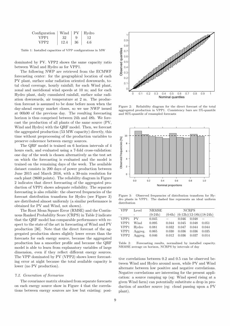
Configuration Wind PV HydroVPP1 32 9 12VPP2 12.4 36 4.6

Table 1: Installed capacities of VPP configurations in MW

dominated by PV. VPP2 shows the same capacity ratiobetween Wind and Hydro as for VPP1.

The following NWP are retrieved from the ECMWFforecasting center: for the geographical location of eachPV plant, surface solar radiation oriented downwards, to-tal cloud coverage, hourly rainfall; for each Wind plant,zonal and meridional wind speeds at 10 m; and for eachHydro plant, daily cumulated rainfall, surface solar radi-ation downwards, air temperature at 2 m. The produc-tion forecast is assumed to be done before noon when theday-ahead energy market closes, so we use NWP issuedat 00h00 of the previous day. The resulting forecastinghorizon is thus comprised between 24h and 48h. We fore-cast the production of all plants of the same source (PV,Wind and Hydro) with the QRF model. Then, we forecastthe aggregated production (53 MW capacity) directly, thistime without preprocessing of the production variables topreserve coherence between energy sources.

The QRF model is trained on 6 horizon intervals of 4hours each, and evaluated using a 7-fold cross-validation:one day of the week is chosen alternatively as the test seton which the forecasting is evaluated and the model istrained on the remaining days of the week. The availabledataset consists in 200 days of power production betweenJune 2015 and March 2016, with a 30-min resolution foreach plant (9600 points). The reliability diagram in Figure2 indicates that direct forecasting of the aggregated pro-duction of VPP1 shows adequate reliability. The separateforecasting is also reliable: the observed frequencies of theforecast distribution transform for Hydro (see Figure 3)are distributed almost uniformly (a similar performance isobtained for PV and Wind, not shown).

The Root Mean Square Error (RMSE) and the Contin-uous Ranked Probability Score (CRPS) in Table 2 indicatethat the QRF model has comparable performance with re-spect to the state of the art in forecasting of Wind and PVproduction [36]. Note that the direct forecast of the ag-gregated production shows slightly lower errors than theforecasts for each energy source, because the aggregatedproduction has a smoother profile and because the QRFmodel is able to learn from explanatory variables of largedimension, even if they reflect different energy sources.The VPP dominated by PV (VPP2) shows lower forecast-ing error at night because the total available capacity islower (no PV production).

7.2. Generation of Scenarios

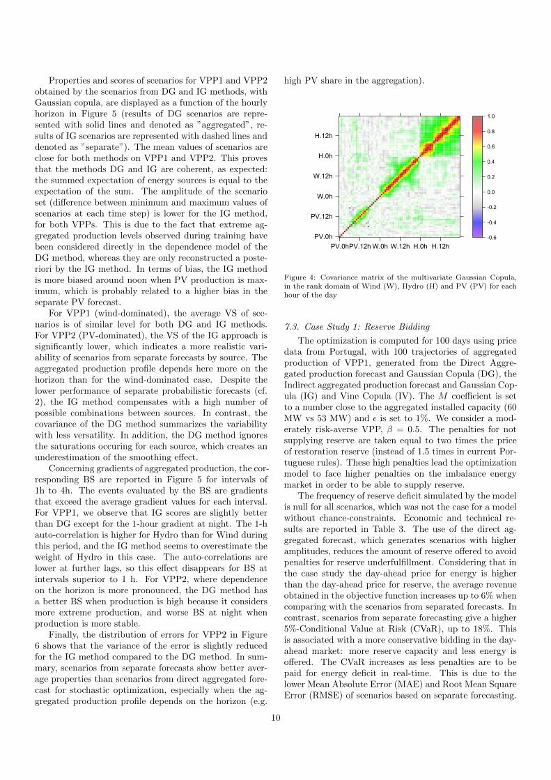
The covariance matrix obtained from separate forecastson each energy source show in Figure 4 that the correla-tions between energy sources are low but existing: posi-

0

0.1

0.2

0.3

0.4

0.5

0.6

0.7

0.8

0.9

1

0 0.1 0.2 0.3 0.4 0.5 0.6 0.7 0.8 0.9 1Nominal quantiles

Obs

erve

d qu

antil

es

Figure 2: Reliability diagram for the direct forecast of the totalaggregated production in VPP1. Consistency bars are 5%-quantileand 95%-quantile of resampled forecasts

Nominal proportions

Obs

erve

d fr

eque

ncie

s [%

]

0

2

4

6

8

10

0.0 0.2 0.4 0.6 0.8 1.0

Figure 3: Observed frequencies of distribution transform for Hy-dro plants in VPP1. The dashed line represents an ideal uniformdistribution

VPP Level NRMSE NCRPS- - (0-24h) (0-6h) (6-12h)(12-18h)(18-24h)VPP1 PV 0.045 − 0.046 0.048 −VPP1 Wind 0.095 0.044 0.045 0.048 0.051VPP1 Hydro 0.081 0.032 0.047 0.044 0.044VPP1 Aggreg. 0.065 0.030 0.036 0.036 0.035VPP2 Aggreg. 0.046 0.012 0.036 0.037 0.014

Table 2: Forecasting results, normalized by installed capacity.NRMSE average on horizon, NCRPS by intervals of day

tive correlations between 0.2 and 0.5 can be observed be-tween Wind and Hydro around noon, while PV and Windalternate between low positive and negative correlations.Negative correlations are interesting for the present appli-cation: a source ramping up (eg: Wind speed rising at agiven Wind farm) can potentially substitute a drop in pro-duction of another source (eg: cloud passing upon a PVplant).

9

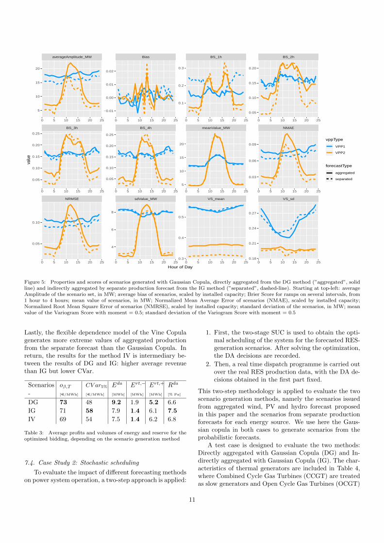
Properties and scores of scenarios for VPP1 and VPP2obtained by the scenarios from DG and IG methods, withGaussian copula, are displayed as a function of the hourlyhorizon in Figure 5 (results of DG scenarios are repre-sented with solid lines and denoted as ”aggregated”, re-sults of IG scenarios are represented with dashed lines anddenoted as ”separate”). The mean values of scenarios areclose for both methods on VPP1 and VPP2. This provesthat the methods DG and IG are coherent, as expected:the summed expectation of energy sources is equal to theexpectation of the sum. The amplitude of the scenarioset (difference between minimum and maximum values ofscenarios at each time step) is lower for the IG method,for both VPPs. This is due to the fact that extreme ag-gregated production levels observed during training havebeen considered directly in the dependence model of theDG method, whereas they are only reconstructed a poste-riori by the IG method. In terms of bias, the IG methodis more biased around noon when PV production is max-imum, which is probably related to a higher bias in theseparate PV forecast.

For VPP1 (wind-dominated), the average VS of sce-narios is of similar level for both DG and IG methods.For VPP2 (PV-dominated), the VS of the IG approach issignificantly lower, which indicates a more realistic vari-ability of scenarios from separate forecasts by source. Theaggregated production profile depends here more on thehorizon than for the wind-dominated case. Despite thelower performance of separate probabilistic forecasts (cf.2), the IG method compensates with a high number ofpossible combinations between sources. In contrast, thecovariance of the DG method summarizes the variabilitywith less versatility. In addition, the DG method ignoresthe saturations occuring for each source, which creates anunderestimation of the smoothing effect.

Concerning gradients of aggregated production, the cor-responding BS are reported in Figure 5 for intervals of1h to 4h. The events evaluated by the BS are gradientsthat exceed the average gradient values for each interval.For VPP1, we observe that IG scores are slightly betterthan DG except for the 1-hour gradient at night. The 1-hauto-correlation is higher for Hydro than for Wind duringthis period, and the IG method seems to overestimate theweight of Hydro in this case. The auto-correlations arelower at further lags, so this effect disappears for BS atintervals superior to 1 h. For VPP2, where dependenceon the horizon is more pronounced, the DG method hasa better BS when production is high because it considersmore extreme production, and worse BS at night whenproduction is more stable.

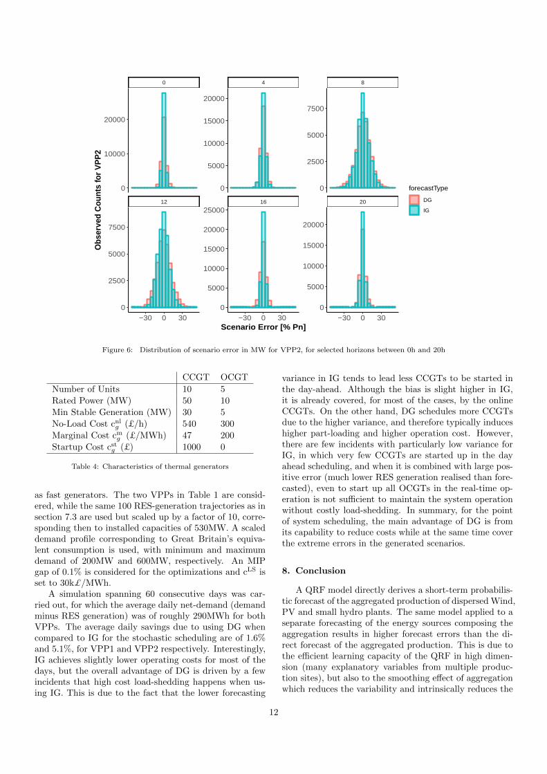
Finally, the distribution of errors for VPP2 in Figure6 shows that the variance of the error is slightly reducedfor the IG method compared to the DG method. In sum-mary, scenarios from separate forecasts show better aver-age properties than scenarios from direct aggregated fore-cast for stochastic optimization, especially when the ag-gregated production profile depends on the horizon (e.g.

high PV share in the aggregation).

PV.0h

PV.12h

W.0h

W.12h

H.0h

H.12h

PV.0hPV.12hW.0h W.12h H.0h H.12h-0.6

-0.4

-0.2

0.0

0.2

0.4

0.6

0.8

1.0

Figure 4: Covariance matrix of the multivariate Gaussian Copula,in the rank domain of Wind (W), Hydro (H) and PV (PV) for eachhour of the day

7.3. Case Study 1: Reserve Bidding

The optimization is computed for 100 days using pricedata from Portugal, with 100 trajectories of aggregatedproduction of VPP1, generated from the Direct Aggre-gated production forecast and Gaussian Copula (DG), theIndirect aggregated production forecast and Gaussian Cop-ula (IG) and Vine Copula (IV). The M coefficient is setto a number close to the aggregated installed capacity (60MW vs 53 MW) and ε is set to 1%. We consider a mod-erately risk-averse VPP, β = 0.5. The penalties for notsupplying reserve are taken equal to two times the priceof restoration reserve (instead of 1.5 times in current Por-tuguese rules). These high penalties lead the optimizationmodel to face higher penalties on the imbalance energymarket in order to be able to supply reserve.

The frequency of reserve deficit simulated by the modelis null for all scenarios, which was not the case for a modelwithout chance-constraints. Economic and technical re-sults are reported in Table 3. The use of the direct ag-gregated forecast, which generates scenarios with higheramplitudes, reduces the amount of reserve offered to avoidpenalties for reserve underfulfillment. Considering that inthe case study the day-ahead price for energy is higherthan the day-ahead price for reserve, the average revenueobtained in the objective function increases up to 6% whencomparing with the scenarios from separated forecasts. Incontrast, scenarios from separate forecasting give a higher5%-Conditional Value at Risk (CVaR), up to 18%. Thisis associated with a more conservative bidding in the day-ahead market: more reserve capacity and less energy isoffered. The CVaR increases as less penalties are to bepaid for energy deficit in real-time. This is due to thelower Mean Absolute Error (MAE) and Root Mean SquareError (RMSE) of scenarios based on separate forecasting.

10

NRMSE sdValue_MW VS_mean VS_sd

BS_3h BS_4h meanValue_MW NMAE

averageAmplitude_MW Bias BS_1h BS_2h

0 5 10 15 20 25 0 5 10 15 20 25 0 5 10 15 20 25 0 5 10 15 20 25

0 5 10 15 20 25 0 5 10 15 20 25 0 5 10 15 20 25 0 5 10 15 20 25

0 5 10 15 20 25 0 5 10 15 20 25 0 5 10 15 20 25 0 5 10 15 20 25

0.05

0.10

0.15

0.20

0.03

0.06

0.09

0.18

0.21

0.24

0.27

0.1

0.2

0.3

5

10

15

20

0.3

0.4

0.5

−0.01

0.00

0.01

0.02

0.05

0.10

0.15

0.20

0.25

4

6

8

5

10

15

20

0.05

0.10

0.15

0.20

0.25

0.05

0.10

Hour of Day

valu

e

vppType

VPP1

VPP2

forecastType

aggregated

separated

Figure 5: Properties and scores of scenarios generated with Gaussian Copula, directly aggregated from the DG method (”aggregated”, solidline) and indirectly aggregated by separate production forecast from the IG method (”separated”, dashed-line). Starting at top-left: averageAmplitude of the scenario set, in MW; average bias of scenarios, scaled by installed capacity; Brier Score for ramps on several intervals, from1 hour to 4 hours; mean value of scenarios, in MW; Normalized Mean Average Error of scenarios (NMAE), scaled by installed capacity;Normalized Root Mean Square Error of scenarios (NMRSE), scaled by installed capacity; standard deviation of the scenarios, in MW; meanvalue of the Variogram Score with moment = 0.5; standard deviation of the Variogram Score with moment = 0.5

Lastly, the flexible dependence model of the Vine Copulagenerates more extreme values of aggregated productionfrom the separate forecast than the Gaussian Copula. Inreturn, the results for the method IV is intermediary be-tween the results of DG and IG: higher average revenuethan IG but lower CVar.

Scenarios oβ,T CV ar5% Eda Ert,− Ert,+ Rda

- [€/MWh] [€/MWh] [MWh] [MWh] [MWh] [% Pn]

DG 73 48 9.2 1.9 5.2 6.6

IG 71 58 7.9 1.4 6.1 7.5

IV 69 54 7.5 1.4 6.2 6.8

Table 3: Average profits and volumes of energy and reserve for theoptimized bidding, depending on the scenario generation method

7.4. Case Study 2: Stochastic scheduling

To evaluate the impact of different forecasting methodson power system operation, a two-step approach is applied:

1. First, the two-stage SUC is used to obtain the opti-mal scheduling of the system for the forecasted RES-generation scenarios. After solving the optimization,the DA decisions are recorded.

2. Then, a real time dispatch programme is carried outover the real RES production data, with the DA de-cisions obtained in the first part fixed.

This two-step methodology is applied to evaluate the twoscenario generation methods, namely the scenarios issuedfrom aggregated wind, PV and hydro forecast proposedin this paper and the scenarios from separate productionforecasts for each energy source. We use here the Gaus-sian copula in both cases to generate scenarios from theprobabilistic forecasts.

A test case is designed to evaluate the two methods:Directly aggregated with Gaussian Copula (DG) and In-directly aggregated with Gaussian Copula (IG). The char-acteristics of thermal generators are included in Table 4,where Combined Cycle Gas Turbines (CCGT) are treatedas slow generators and Open Cycle Gas Turbines (OCGT)

11

12 16 20

0 4 8

−30 0 30 −30 0 30 −30 0 30

0

2500

5000

7500

0

5000

10000

15000

20000

0

5000

10000

15000

20000

0

5000

10000

15000

20000

25000

0

10000

20000

0

2500

5000

7500

Scenario Error [% Pn]

Obs

erve

d C

ount

s fo

r VP

P2

forecastType

DG

IG

Figure 6: Distribution of scenario error in MW for VPP2, for selected horizons between 0h and 20h

CCGT OCGT

Number of Units 10 5

Rated Power (MW) 50 10

Min Stable Generation (MW) 30 5

No-Load Cost cnlg (£/h) 540 300

Marginal Cost cmg (£/MWh) 47 200

Startup Cost cstg (£) 1000 0

Table 4: Characteristics of thermal generators

as fast generators. The two VPPs in Table 1 are consid-ered, while the same 100 RES-generation trajectories as insection 7.3 are used but scaled up by a factor of 10, corre-sponding then to installed capacities of 530MW. A scaleddemand profile corresponding to Great Britain’s equiva-lent consumption is used, with minimum and maximumdemand of 200MW and 600MW, respectively. An MIPgap of 0.1% is considered for the optimizations and cLS isset to 30k£/MWh.

A simulation spanning 60 consecutive days was car-ried out, for which the average daily net-demand (demandminus RES generation) was of roughly 290MWh for bothVPPs. The average daily savings due to using DG whencompared to IG for the stochastic scheduling are of 1.6%and 5.1%, for VPP1 and VPP2 respectively. Interestingly,IG achieves slightly lower operating costs for most of thedays, but the overall advantage of DG is driven by a fewincidents that high cost load-shedding happens when us-ing IG. This is due to the fact that the lower forecasting

variance in IG tends to lead less CCGTs to be started inthe day-ahead. Although the bias is slight higher in IG,it is already covered, for most of the cases, by the onlineCCGTs. On the other hand, DG schedules more CCGTsdue to the higher variance, and therefore typically induceshigher part-loading and higher operation cost. However,there are few incidents with particularly low variance forIG, in which very few CCGTs are started up in the dayahead scheduling, and when it is combined with large pos-itive error (much lower RES generation realised than fore-casted), even to start up all OCGTs in the real-time op-eration is not sufficient to maintain the system operationwithout costly load-shedding. In summary, for the pointof system scheduling, the main advantage of DG is fromits capability to reduce costs while at the same time coverthe extreme errors in the generated scenarios.

8. Conclusion

A QRF model directly derives a short-term probabilis-tic forecast of the aggregated production of dispersed Wind,PV and small hydro plants. The same model applied to aseparate forecasting of the energy sources composing theaggregation results in higher forecast errors than the di-rect forecast of the aggregated production. This is due tothe efficient learning capacity of the QRF in high dimen-sion (many explanatory variables from multiple produc-tion sites), but also to the smoothing effect of aggregationwhich reduces the variability and intrinsically reduces the

12

uncertainty in production. An extension of this work couldconsist in forecasting the multi-source aggregated produc-tion with a deep quantile regression approach, with theobjective to outperform the performance of the machinelearning model used here and scale to potentially largeraggregations.

Scenarios of aggregated production have been gener-ated from these probabilistic forecasts. The impact ofchoosing either a direct forecast of the aggregated pro-duction or a separate forecast for each energy source isassessed on two power system applications requiring suchscenarios. A multivariate copula, of type either Gaussianor Vine, is applied to obtain scenarios from the day-aheadproduction forecasts. The generation methods are evalu-ated on two different aggregations with different capacityshares for the different energy sources.

It is found on one hand that scenarios from the ag-gregated forecast have a higher amplitude, because thescenario generation method incorporates directly past ex-treme levels of aggregated production, meanwhile scenar-ios from separate forecasts reconstruct extreme aggregatedlevels from the marginal contributions of each source in theaggregation. On the other hand, scenarios issued from theseparate forecasting of each source reproduce more accu-rately the variability of the aggregated production whenthe production is highly dependent on the horizon, for in-stance when PV is dominant in the total production. Thisis quantified by a sensible gain on the Variogram Score forthe PV-dominated aggregation, whereas the gain is closeto zero for a Wind-dominated aggregation. This is due toa better reproduction of the various conditions leading tothe observed smoothing effect in aggregated production.In this case the available information about the variabilityfor each source is preserved, whereas a given level of to-tal production can arise from multiple distinct productionpatterns at the level of each source, hence loosing infor-mation on the diversity of production profiles.

When used in both stochastic applications of reservebidding and unit commitment, scenarios from direct ag-gregated production forecast generate more average value(increased profit or reduced costs) than those from sepa-rate forecasts, because these applications are sensible tothe amplitude of the scenario set. Extreme levels of aggre-gated production are more present in the scenarios fromdirect aggregated production forecast, which can securehighly risk-averse decisions (e.g. unit commitment underextreme RES aggregated production) but also hinders de-cisions that could be valuable for the agent (e.g. scenar-ios of high amplitude will limit the offer of reserve of anaggregator, with a possible opportunity cost if activatedreserve would have increased his revenue). Finally, a mod-erately risk-averse decision maker will observe that scenar-ios generated from separate forecasts create less penaltiesdue to their sharper distribution and more realistic vari-ability: an aggregator bidding AS and energy will increasehis Conditional Value -at-Risk, and a system operator willdecrease his lower operational costs for most days of the

year. In conclusion, the assessment of scenario generationmethodologies in this paper informs the decision-makerson the optimal way to generate short-term scenarios of ag-gregated RES production according to their risk aversionand to the contribution of each source in the aggregation.

References

[1] M. Yin, Y. Xu, C. Shen, J. Liu, Z. Y. Dong, Y. Zou, TurbineStability-Constrained Available Wind Power of Variable SpeedWind Turbines for Active Power Control, IEEE Transactions onPower Systems 32 (3) (2017) 2487–2488. doi:10.1109/TPWRS.

2016.2605012.[2] L. Spitalny, D. Unger, J. M. A. Myrzik, Potential of small hy-

dro power plants for delivering control energy in Germany, in:2012 IEEE Energytech, IEEE, 2012, pp. 1–6. doi:10.1109/

EnergyTech.2012.6304700.URL http://ieeexplore.ieee.org/document/6304700/

[3] A. F. Hoke, M. Shirazi, S. Chakraborty, E. Muljadi, D. Mak-simovic, Rapid Active Power Control of Photovoltaic Systemsfor Grid Frequency Support, IEEE Journal of Emerging andSelected Topics in Power Electronics 5 (3) (2017) 1154–1163.doi:10.1109/JESTPE.2017.2669299.

[4] A. Gonzalez-Garrido, A. Saez-de Ibarra, H. Gaztanaga, A. Milo,P. Eguia, Annual Optimized Bidding and Operation Strategy inEnergy and Secondary Reserve Markets for Solar Plants withStorage Systems, IEEE Transactions on Power Systems 8950 (c)(2018) 1–10. doi:10.1109/TPWRS.2018.2869626.

[5] S. Camal, A. Michiorri, G. Kariniotakis, Optimal offer of auto-matic frequency restoration reserve from a combined PV/WindVirtual Power Plant, IEEE Transactions on Power Systems33 (6) (2018) 6155–6170. doi:10.1109/TPWRS.2018.2847239.

[6] K. Knorr, B. Zimmermann, M. Speckmann, M. Wunderlich,D. Kirchner, F. Steinke, P. Wolfrum, T. Leveringhaus, T. Lager,L. Hofmann, D. Filzek, T. Gobel, B. Kusserow, L. Nicklaus,P. Ritter, Kombikraftwerk 2 Abschlussbericht (August) (2014)218.URL http://www.kombikraftwerk.de/fileadmin/

Kombikraftwerk_2/Abschlussbericht/Abschlussbericht_

Kombikraftwerk2_aug14.pdf

[7] L. Rubino, C. Capasso, O. Veneri, Review on plug-in electric ve-hicle charging architectures integrated with distributed energysources for sustainable mobility, Applied Energy 207 (2017)438–464. doi:10.1016/J.APENERGY.2017.06.097.URL https://www.sciencedirect.com/science/article/pii/

S0306261917308358

[8] D. Dallinger, M. Wietschel, Grid integration of intermittent re-newable energy sources using price-responsive plug-in electricvehicles (6 2012). doi:10.1016/j.rser.2012.02.019.URL https://www.sciencedirect.com/science/article/pii/

S136403211200113X?via%3Dihub

[9] O. Veneri, Technologies and Applications for Smart Chargingof Electric and Plug-in Hybrid Vehicles, Springer, 2017.

[10] L. Hirth, I. Ziegenhagen, Control power and variable re-newables, International Conference on the European EnergyMarket, EEM 50 (2013) 1035–1051. doi:10.1109/EEM.2013.

6607359.URL http://dx.doi.org/10.1016/j.rser.2015.04.180

[11] T. Soares, P. Pinson, T. V. Jensen, H. Morais, Optimal Offer-ing Strategies for Wind Power in Energy and Primary ReserveMarkets, IEEE Transactions on Sustainable Energy 7 (3) (2016)1036–1045. doi:10.1109/TSTE.2016.2516767.

[12] T. Soares, P. Pinson, Renewable energy sources offering flexi-bility through electricity markets, Ph.D. thesis, Technical Uni-versity of Denmark (2017).

[13] H. Fu, Z. Wu, X.-P. Zhang, J. Brandt, Contributing to DSOsEnergy-Reserve Pool: A Chance-Constrained Two-Stage µVPPBidding Strategy, IEEE Power and Energy Technology SystemsJournal 4 (4) (2017) 1–1. doi:10.1109/JPETS.2017.2749256.URL http://ieeexplore.ieee.org/document/8058436/

13

[14] H. Zhang, Z. Hu, E. Munsing, S. J. Moura, Y. Song, Data-driven Chance-constrained Regulation Capacity Offering forDistributed Energy Resources, IEEE Transactions on SmartGriddoi:10.1109/TSG.2018.2809046.URL https://arxiv.org/pdf/1708.05114.pdf

[15] R. Pinto, R. J. Bessa, M. A. Matos, Multi-period flexibilityforecast for low voltage prosumers, Energy 141 (2017) 2251–2263. doi:10.1016/j.energy.2017.11.142.URL https://repositorio.inesctec.pt/bitstream/

123456789/4767/3/P-00N-9Q4.pdf

[16] P. Meibom, R. Barth, B. Hasche, H. Brand, C. Weber,M. O’Malley, Stochastic Optimization Model to Study theOperational Impacts of High Wind Penetrations in Ireland,IEEE Transactions on Power Systems 26 (3) (2011) 1367–1379.doi:10.1109/TPWRS.2010.2070848.URL http://ieeexplore.ieee.org/document/5587912/

[17] F. Bouffard, F. Galiana, Stochastic Security for OperationsPlanning With Significant Wind Power Generation, IEEETransactions on Power Systems 23 (2) (2008) 306–316. doi:

10.1109/TPWRS.2008.919318.URL http://ieeexplore.ieee.org/document/4470561/

[18] J. M. Morales, A. J. Conejo, J. Perez-Ruiz, Economic valua-tion of reserves in power systems with high penetration of windpower, in: 2009 IEEE Power & Energy Society General Meet-ing, IEEE, 2009, pp. 1–1. doi:10.1109/PES.2009.5260229.URL http://ieeexplore.ieee.org/document/5260229/

[19] A. Tuohy, P. Meibom, E. Denny, M. O’Malley, Unit Commit-ment for Systems With Significant Wind Penetration, IEEETransactions on Power Systems 24 (2) (2009) 592–601. doi:

10.1109/TPWRS.2009.2016470.[20] F. Teng, G. Strbac, Full Stochastic Scheduling for Low-Carbon

Electricity Systems, IEEE Transactions on Automation Scienceand Engineering 14 (2) (2017) 461–470. doi:10.1109/TASE.

2016.2629479.URL http://ieeexplore.ieee.org/document/7833096/

[21] K. Bruninx, Improved modeling of unit commitment decisionsunder uncertainty, Ph.D. thesis (2016).URL https://www.mech.kuleuven.be/en/tme/research/

energy_environment/Pdf/doctoraat-kenneth-bruninx.pdf

[22] P. Pinson, R. Girard, Evaluating the quality of scenarios ofshort-term wind power generation, Applied Energy 96 (2012)12–20. doi:10.1016/j.apenergy.2011.11.004.

[23] F. Golestaneh, H. B. Gooi, P. Pinson, Generation and evalu-ation of spacetime trajectories of photovoltaic power, AppliedEnergy 176 (2016) 80–91. doi:10.1016/J.APENERGY.2016.05.

025.URL https://www.sciencedirect.com/science/article/pii/

S0306261916306079

[24] Z. Wang, W. Wang, C. Liu, Z. Wang, Y. Hou, ProbabilisticForecast for Multiple Wind Farms Based on Regular Vine Cop-ulas, IEEE Transactions on Power Systems 33 (1) (2018) 578–589. doi:10.1109/TPWRS.2017.2690297.URL http://ieeexplore.ieee.org/document/7909035/

[25] W. Wu, K. Wang, B. Han, G. Li, X. Jiang, M. L. Crow, A Ver-satile Probability Model of Photovoltaic Generation Using PairCopula Construction, IEEE Transactions on Sustainable En-ergy 6 (4) (2015) 1337–1345. doi:10.1109/TSTE.2015.2434934.

[26] M. P. Cote, C. Genest, A copula-based risk aggregation model,Canadian Journal of Statistics 43 (1) (2015) 60–81. doi:10.

1002/cjs.11238.URL http://doi.wiley.com/10.1002/cjs.11238

[27] J. Dong, T. Kuruganti, S. M. Djouadi, Very Short-term Photo-voltaic Power Forecasting using Uncertain Basis Function, In-formation Sciences and Systems (CISS), 2017 51st Annual Con-ference on (2017) 1–6.

[28] S. I. Vagropoulos, E. G. Kardakos, C. K. Simoglou, A. G.Bakirtzis, J. P. S. Catalao, ANN-based scenario generationmethodology for stochastic variables of electric power sys-tems, Electric Power Systems Research 134 (2016) 9–18.doi:10.1016/j.epsr.2015.12.020.URL https://ac.els-cdn.com/S0378779615003971/

1-s2.0-S0378779615003971-main.pdf?_tid=

28d90c9a-f6b3-11e7-b494-00000aacb361&acdnat=

1515663681_181743d500e10436507caa9e7c9cf4be

[29] Y. Chen, Y. Wang, D. Kirschen, B. Zhang, Model-Free Renew-able Scenario Generation Using Generative Adversarial Net-works, IEEE Transactions on Power Systems 33 (3) (2018)3265–3275. doi:10.1109/TPWRS.2018.2794541.URL http://ieeexplore.ieee.org/document/8260947/http:

//arxiv.org/abs/1707.09676

[30] N. T. Tung, J. Z. Huang, Thuy Thi Nguyen, I. Khan, Bias-corrected Quantile Regression Forests for high-dimensionaldata, in: 2014 International Conference on Machine Learningand Cybernetics, IEEE, 2014, pp. 1–6. doi:10.1109/ICMLC.

2014.7009082.URL http://ieeexplore.ieee.org/lpdocs/epic03/wrapper.

htm?arnumber=7009082

[31] Y. Zhang, J. Wang, X. Wang, Review on probabilistic fore-casting of wind power generation, Renewable and SustainableEnergy Reviews 32 (2014) 255–270. doi:10.1016/j.rser.2014.01.033.URL http://dx.doi.org/10.1016/j.rser.2014.01.033

[32] L. Ruschendorf, Mathematical Risk Analysis, Vol. 2013, 2013.doi:10.1007/978-3-642-33590-7.URL http://link.springer.com/10.1007/

978-3-642-33590-7

[33] M. Scheuerer, T. M. Hamill, Variogram-Based Proper ScoringRules for Probabilistic Forecasts of Multivariate Quanti-ties*, Monthly Weather Review 143 (4) (2015) 1321–1334.doi:10.1175/MWR-D-14-00269.1.URL https://www.esrl.noaa.gov/psd/people/michael.

scheuerer/variogram-score.pdfhttp://journals.ametsoc.

org/doi/10.1175/MWR-D-14-00269.1

[34] A. E. R. T. T. B. 50hz, Amprion, Consultation on the designof the platform for automatic Frequency Restoration Reserve(aFRR) of PICASSO region.URL https://www.entsoe.eu/Documents/

Networkcodesdocuments/Implementation/picasso/

PICASSO-Consultation_document.pdf?Web=1

[35] C. Liu, X. Wang, Y. Zou, H. Zhang, W. Zhang, A probabilis-tic chance-constrained day-ahead scheduling model for grid-connected microgrid, in: 2017 North American Power Sym-posium, NAPS 2017, no. 51577146, 2017. doi:10.1109/NAPS.

2017.8107180.[36] G. Kariniotakis, Renewable Energy Forecasting - From Models

to Applications, Woodhead Publishing Series in Energy, Wood-head Publishing Series in Energy - Elsevier, 2017.

14