Scattering bright solitons: Quantum versus mean-field behavior

Scattering bright solitons: quantum versus mean-field behavior

Bettina Gertjerenken,1, ∗ Thomas P. Billam,2, 3 Lev Khaykovich,4 and Christoph Weiss1, 2

1Institut fur Physik, Carl von Ossietzky Universitat, D-26111 Oldenburg, Germany2Department of Physics, Durham University, Durham DH1 3LE, United Kingdom

3Jack Dodd Center for Quantum Technology, Department of Physics,University of Otago, Dunedin 9016, New Zealand

4Department of Physics, Bar-Ilan University, Ramat-Gan, 52900 Israel(Dated: 03 September 2012)

We investigate scattering bright solitons off a potential using both analytical and numerical meth-ods. Our paper focuses on low kinetic energies for which differences between the mean-field descrip-tion via the Gross-Pitaevskii equation (GPE) and the quantum behavior are particularly large. Onthe N -particle quantum level, adding an additional harmonic confinement leads to a simple signa-ture to distinguish quantum superpositions from statistical mixtures. While the non-linear characterof the GPE does not allow quantum superpositions, the splitting of GPE-solitons takes place onlypartially. When the potential strength is increased, the fraction of the soliton which is transmittedor reflected jumps non-continuously. We explain these jumps via energy-conservation and interpretthem as indications for quantum superpositions on the N -particle level. On the GPE-level, we alsoinvestigate the transition from this stepwise behavior to the continuous case.

PACS numbers: 03.75.Gg, 03.75.Lm, 34.50.Cx, 03.65.SqKeywords: mesoscopic quantum superpositions, bright solitons, beyond-mean-field behavior

I. INTRODUCTION

Bright solitons generated from attractively interactingultra-cold atoms have been realized experimentally bothin quasi one-dimensional (1D) configurations [1, 2] andthree dimensions (3D) [3].

Some of the effects investigated for bright solitons [4]could, in principle, also be investigated in classical sys-tems. However, bright quantum-matter-wave solitons aremesoscopic quantum objects which are particularly use-ful to investigate beyond mean-field effects of quantumsolitons: While there are cases for which both the classi-cal and quantum descriptions agree for particle numbersas low as N ' 3 [5], it has been proposed to use scat-tering bright solitons off a potential in order to producenon-classical quantum superpositions [6, 7].

Other investigations of bright solitons include sta-tionary solutions of the (mean field) Gross-Pitaevskiiequation (GPE) [8], soliton trains [9, 10], solitons un-der transverse confinement [11] and incoherent matter-wave solitons [12] as well as deviation from one dimen-sionality [13] and regular and chaotic dynamics in soli-ton collisions [14]. Research also covers topics rangingfrom fragmented states [15], stabilization and destabiliza-tion of second-order solitons against perturbations [16]and quantum reflections [17] over soliton localizationvia disorder [18, 19] and in time-dependent traps withtime-dependent scattering length [20], resonant trappingthrough a quantum well [21] and possible applications tointerferometry [22–24].

The focus of the present paper lies on scattering brightsolitons off a potential in a one-dimensional geometry.

∗ [email protected]

On the N -particle quantum level this can result in quan-tum superpositions; however, the detection of such super-positions requires the identification of a clear experimen-tal signature. For mean-field solitons both behavior sim-ilar to the case of a single particle (see, e.g., Ref. [23, 24])and considerably deviating behavior has been reported inthe literature.1 By focusing on low kinetic energies, wewill discuss the parameter regimes for which both typesof behavior can be expected.

The paper is organized as follows: Section II introducesthe models used to investigate scattering bright solitonsoff scattering potentials. The energetically allowed finalstates are discussed in Sec. III.

In Sec. IV, scattering bright solitons off a scatteringpotential is investigated with additional harmonic con-finement as used in experiment [26]. Section V explainsthe behavior on the level of the GPE. Section VI con-cludes the paper.

II. MODELS

On the level of the N -particle quantum mechan-ics, the system can be described by the Lieb-Liniger(-McGuire) [27, 28] Hamiltonian with additional external

1 Scattering mean-field (GPE) solitons off a barrier with behav-ior that considerably deviates from a single particle has beeninvestigated both in Ref. [25] and on page 2 of Ref. [7].

arX

iv:1

208.

2941

v2 [

cond

-mat

.qua

nt-g

as]

4 S

ep 2

012

2

potential Vext:

H =−N∑j=1

~2

2m∂2xj

+

N−1∑j=1

N∑n=j+1

g1Dδ (xj − xn)

+

N∑j=1

Vext (xj) , (1)

with g1D < 0.The mean-field equation corresponding to the Hamil-

tonian (1) is the GPE [4]

i~∂tϕ(x, t) =− ~2

2m∂2xϕ(x, t) + Vext(x)ϕ(x, t)

+ (N − 1)g1D|ϕ(x, t)|2ϕ(x, t) , (2)

where |ϕ(x, t)|2 is the single-particle density (cf. [29]).While the GPE (2) often is used to describe Bose-Einsteincondensates (BECs) of finite particle numbers, it canstrictly speaking only be valid in the limit [29]:

N → ∞g1D → 0

with Ng1D = const. (3)

There even are cases for which the Gross-Pitaevskii func-tional becomes exact in this limit [29].

For attractive interactions and without an external po-tential [Vext(x) ≡ 0], Eq. (2) has exact soliton solutionsof the form [4]

ϕ(x, 0) =

√2µ

(N − 1)g1D

eimµx/~−i(µ−mu2/2)t/~

cosh

[√2m|µ|~2 (x− x0 − ut)

] ,(4)

where u is the velocity and x0 the initial position. Onthe one hand, Eq. (4) describes a single soliton, for whichnormalizing Eq. (4) to one yields (cf. [30])

µ = −1

8

mg21D

~2(N − 1)2 . (5)

On the other hand, Eq. (4) can also describe (well sepa-rated) parts of a solution. The sum of two such solutionswhich are, e.g., on both sides of a scattering potentialcorresponds to a fraction of the atoms being on one sideand the rest of the atoms on the other side (note thatthe widths of the two solitons then depends on whichfraction of the atoms is on each side). This is, however,very different from a quantum superposition of one soli-ton containing all atoms being simultaneously on bothsides (cf. [6]).

Contrary to the localized mean-field solution (4),eigensolutions of the N -particle Schrodinger equationcorresponding to the Hamiltonian (1) with zero externalpotential Vext have to be translationally invariant (up toa phase factor):

ψN (x, t) ∝ exp

−β N−1∑j=1

N∑n=j+1

|xj − xn|+ ik

N∑j=1

xj

(6)

with

β ≡ m|g1D|2~2

. (7)

The eigenenergy E = E0(N) + Ekin of the eigenfunc-tion (6) consists of the ground-state energy

E0(N) = − 1

24

mg21D

~2N(N2 − 1) (8)

and the center-of-mass kinetic energy

Ekin = N~2k2

2m. (9)

On the one hand, there are cases for which mean-fieldand N -particle physics can be shown to agree: By as-suming the center-of-mass part of the wave function tobe a delta function,

ψC(X) = δ(X − x0 − ut) ,it is possible to show that the single-particle density ofthe Gross-Pitaevskii soliton (4) and the many-particlesoliton (6) coincide in the limit N 1 [31]. Thus, ratherthan simply being the solution of an approximated equa-tion, the single-particle density of exact many-particlesolitons (6) is well described by the mean-field case (4).

On the other hand, there are cases for which there isno equivalent on the mean-field (GPE) level: Mesoscopicquantum superpositions.

III. MESOSCOPIC QUANTUMSUPERPOSITIONS (MQS) VS.HARTREE-PRODUCT STATES

As a starting point to investigate mesoscopic quan-tum superpositions (MQS), this section first investigatesparameter regimes accessible to the N -particle physicswhen scattering a bright quantum soliton off a poten-tial by looking at the energetically allowed final states inthe N -particle case (Sec. III A) after the soliton has leftthe potential. Section III B investigates Hartree-productstates of the form

ψ(x, t) =

N∏j=1

ϕ(xj , t) . (10)

A. N-particle quantum mechanics

It has been suggested that scattering slow bright quan-tum solitons of N ≈ 100 particles off a scattering poten-tial generates mesoscopic quantum superpositions [6, 7].Scattering would produce a quantum superposition of allparticles being either on one side of the scattering poten-tial or at the other side:

|ψ〉MQS =1√2

(|N, 0〉+ eiα|0, N〉

)(11)

3

FIG. 1. (Color online) Energetically (dis)allowed states forN = 100 particles with n particles on one side of the scatter-ing potential and N −n particles on other side. The parame-ter regions are displayed as a function of n and center-of-masskinetic energy Ekin. (a) Magenta/gray region: not energet-ically allowed as soon as all particles have left the scatter-ing potential, black and white regions: energetically allowed.Only in the white region [which lies above Ekin ' 0.755|E0|for N = 100; Eq. (14)] are product states with 50:50 occu-pation on both side of the barrier energetically allowed. (b)Enhanced lower part of the left panel. In the energy regimebelow the dashed line, the only energetically allowed statesare: all particles on the left or all particles on the right of thebarrier – and quantum superpositions of both.

where the Fock-state notation |N − n, n〉 denotes N − nparticles on the right and n particles on the left ofthe scattering potential. Such states have been called“Schrodinger-cat states” or “NOON states”; further sug-gestions how mesoscopic quantum superpositions mightbe obtained can be found, e.g., in Refs. [32–42].

MQS can be more general than Eq. (11); quantum su-perposition involving states like

|ψ〉n =1√2

(|N − n, n〉+ eiα|n,N − n〉

), n /

N

4(12)

or superpositions thereof are also interesting. Further-more, quantum superpositions which do not correspondto exact 50:50 splitting are also in the focus of research(cf. [7]).

Figure 1 depicts the possible energy regimes. For highcenter-of-mass kinetic energy [well in the white area ofFig. 1 (a), the parameter regime investigated, e.g., inRefs. [23, 24]],

Ekin 2E0

(N

2

)− E0(N) , (13)

the soliton is energetically allowed to break into (at least)2 parts. The scattering potential can act as a beam split-ter on the level of single particles. In this energy regime,the mean-field soliton splits [23, 24], which includes 50:50splitting. In the high energy regime, the particle radia-tion observable at lower energies disappears [43] and thesystem thus stays condensed. Replacing the “” by “=”in Eq. (13) yields the value for the boundary between the

white and the black region in Fig. 1 (a):

Ekin

' −0.755E0 : N = 100= −0.75E0 : N →∞ . (14)

For low center-of-mass kinetic energies [below thedashed line in Fig. 1 (b)],

Ekin < E0(N − 1)− E0(N) , (15)

the soliton is energetically forbidden to break into twoparts and thus all particles are either on one side of thescattering potential (n = 0) or on the other (n = N);quantum superpositions of both (11) have been pre-dicted [6].

In between the threshold given by Eqs. (14) and(15), contributions of more states are allowed; the ma-genta/gray region indicates which |N − n, n〉 are ener-getically disallowed for each value of the center-of-masskinetic energy. Contributions of states like |N/2, N/2〉automatically imply that this part of the wave functionhas a higher energy than energetically allowed for any pa-rameter regime which is labeled magenta/gray in Fig. 1.This statement is independent of the N -particle statethese particles are in as long as they cannot be found atthe potential.

On the N -particle level governed by the Hamilto-nian (1), energy is conserved not only in the sense that

〈ψ(t)|H|ψ(t)〉 is conserved but also in the sense that all

higher moments 〈ψ(t)|Hν |ψ(t)〉, ν = 2, 3, . . . are time-independent2. Thus, within the magenta/gray param-eter regime depicted in Fig. 1 energy conservation notonly prevents the final state from being identical to|N/2, N/2〉, but |N/2, N/2〉 (and, |N/2−n,N/2+n〉 withincreasing n for decreasing initial center-of-mass kineticenergy) cannot even be an important contribution to thefinal wave function.

Just because a certain value for n is energetically al-lowed does not necessarily imply that it will occur: at thethreshold given by Eq. (14), n = N/2 could, in principleoccur. However, this would imply that in the final state,the fractions of the soliton on both sides of the barrierno longer move. It is thus more likely to occur for evenhigher initial center-of-mass kinetic energies.

B. Mean-field approach via Hartree-product states

Often, mean-field theories are introduced [4] forbosonic N -particle quantum systems by starting with

2 As the time-evolution operator U(t, 0) = exp(−iHt/~) (with

|ψ(t)〉 = U(t, 0)|ψ(0)〉) commutes with Hν (ν = 1, 2, 3, . . .), we

have: 〈ψ(t)|Hν |ψ(t)〉 = 〈ψ(0)|Hν |ψ(0)〉 for ν = 2, 3, 4, . . .. Thisexcludes contributions from eigenfunctions for which the eigenen-ergy is not negative enough to contribute to the final state. Alter-natively, Hν could be replaced by [H−E0(N)]ν before repeatingthis analysis.

4

Hartree-product states (10), which are subsequently usedto derive Gross-Pitaevskii equations like Eq. (2) [4]. Thisdoes, however, not necessarily imply that GPE is equiva-lent to the Hartree-product states; rather than interpret-ing the GPE-solution φ(x, t) automatically as being partof a Hartree-wave function, a more general approach isto regard |φ(x, t)|2 as the “single-particle density” [29].

Hartree-product states for which ϕ(x, t) is zero on oneside of the potential always exist. More interesting tocompare with Sec. III A are wave functions for whichϕ(x, t) is non-zero on both sides of the scattering po-tential. In this case, both the Fock-state |N/2, N/2〉 and|N/2+n,N/2−n〉 (with small n) are thus involved in themany-particle Hartree-product wave function: All Fockstates contribute to the wave-function [as long as thesingle-particle wave function is non-zero at both sides,cf. Eq. (A9)]. Note that contrary to the case of Hartree-product states, contributions of such states to the to-tal wave function can be avoided in the case of a MQS.Strictly speaking, for low center-of-mass kinetic energies,those states are not accessible on the N -particle level (asdiscussed in the previous section). This seems to agreewith the rather stepwise behavior of scattering mean-fieldsolitons reported in Refs. [7, 25]. This paper investigatesthe transition from this stepwise behavior to the continu-ous case similar to single-particle physics in more detail.We will show that Fig. 1 provides the energy scale onwhich the non-splitting GPE-soliton becomes a splittingsoliton, depending on its initial center-of-mass energy.The technical details are presented in Appendix A.

IV. SCATTERING DYNAMICS IN THEPRESENCE OF HARMONIC CONFINEMENT

A recent (quasi-) 1D experiment [26] so far com-bines scattering solitons off a potential in 1D with addi-tional harmonic confinement. We model this situation inSec. IV A. So far, it does not yet realize the regime of bothlow kinetic energies and temperatures necessary to pro-duce the quantum superpositions suggested in Refs. [6, 7].

For the N -particle quantum case (Sec. IV B), the ideais to start with the many-particle ground state in theharmonic trap (cf. [44]), the center of the trap can then(quasi-)instantaneously be shifted, followed by switchingon the scattering potential in the middle of the trap.For the mean-field description via the GPE (Sec. IV C)the same situation is repeated for a single soliton with-out initial center-of-mass kinetic energy. While thetwo Secs. IV B and IV C cover different energy regimes,Sec. IV D demonstrates what effects can happen, in prin-ciple, on the N -particle level for the parameter-regime forwhich the GPE displays the peculiar behavior discussedin Sec. IV C.

A. Harmonic confinement and scattering potential

We assume the scattering potential to be narrowenough3 for it to be approximated by a delta function:

Vext(x) =1

2mω2x2 + v0δ(x) ; (16)

where “narrow” refers to the potential being narrowerthan both the soliton width (cf. [18, 19]) and the oscilla-tor length:

λGPE ≡(

~mω

) 12

, (17)

where the index GPE indicates that this is a relevantlength scale for the GPE.

B. N-particle quantum physics: effective potentialapproach

The effective potential approach of Ref. [6, 45] is validfor low center-of-mass kinetic energies;4 the system canbe described by an effective Schrodinger equation for thecenter-of-mass coordinate X. This effective Schrodingerequation reads:

i~∂tψC(X, t) =

[− ~2

2Nm∂2X +

1

2Nmω2X2

]ψC(X, t)

+ Veff(X)ψC(X, t) (18)

where the effective potential is given by [6, 45]

Veff(X) =

∫dNx|ψN,k(x)|2V (x)δ

(X− 1

N

∑Nν=1 xν

)≡ U0

cosh2(X/`), (19)

where the last line uses the results of Ref. [31] and theparameters are: the strength

U0 ≡Nv0

4

m|g1D|(N − 1)

~2, (20)

which is the product of the particle number, the single-particle potential strength v0 [Eq. (16)] and the solitonamplitude [Eqs. (4) and (5)] and the width

` ≡ 2~2

m|g1D|(N − 1)(21)

3 Wide potentials were discussed in the N -particle quantum casein Refs. [6, 7].

4 The validity of the effective-potential approach [6, 45] to de-scribe time-dependent scattering has been proved rigorously bycalculating strict bounds on the transmission and reflection am-plitudes [46].

5

given by the soliton width [30], cf. Eq. (5).The effective potential (19) thus has the form of the

soliton; the ratio of the width ` to the center-of-massoscillator length [cf. Eqs. (17) and (18)]

λosc ≡(

~Nmω

) 12

(22)

=λGPE√N

, (23)

influences the physics.As soon as the center-of-mass density near the effective

potential approaches zero, MQS states emerge (cf. [6]).For center-of-mass energies which are an order of magni-tude higher, numerics still predicts quantum superposi-tions far from product states [7].

One advantage of the additional harmonic trapping po-tential is that excitations due to an opening of the trapwhich prepares the initial state [47] can be discarded.Another advantage is discussed in this section: simplyproducing potentially interesting MQS and showing thatin an experiment all particles are either on one side ofthe potential or at the other would not be enough toconfirm the existence of MQS; additional experimentalsignatures are necessary. One possibility is to look at theinterference in the center-of-mass density after removingthe barrier [6].

For not-too-broad effective potentials (19), there is asimpler approach shown in Fig. 2: After the second col-lision of both parts of the wave function in the presenceof the barrier, this leads to a probability close to one ofall particles being at the side opposite to the initial con-dition [Fig. 2 (b)], which considerably differs from thecase of a statistical mixture [Fig. 2 (a)]. Losing a singleparticle after the creation of the quantum superpositionwould turn the MQS (11) into such a mixture. Whilethe precise influence of decoherence will depend on ex-perimental details, we model decoherence by replacingthe quantum superposition of all atoms being either onone side of the scattering potential or on the other by astatistical mixture near t ≈ T/2.

In order to understand this behavior, let us first assumethe scattering potential is narrow enough to be approxi-mated by a delta function:

Veff(X) =~2

mΩδ(x+ xs). (24)

where we included a small shift to the left.In order to derive the leading order behavior of our

center-of-mass wave packet, start with the fact that with-out the scattering potential, after some time the wavepacket would be in the middle of the potential with allthe initial potential energy being transformed into ki-netic energy. For a plane wave with wavevector k, thetransmission coefficient is given by [49]

T =ik

ik − Ω(25)

(b)

x/λosct/T

−15 0 150

0.5

1

(a)

t/T

−15 0 150

0.5

1

|Ψ|2

[arb.units]

0

1

FIG. 2. (Color online) Center-of-mass density of a 1D brightquantum-matter-wave soliton in a two-dimensional projectionas a function of both time t (in units of the oscillation periodT ) and elongation x (in units of the oscillator length λosc).There is additional harmonic confinement (∝ x2); the soli-ton is modeled within the effective potential approach. Ini-tially, the wave function is centered around x = −10λosc.At t = 0.25T the soliton scatters off a narrow effective po-tential modeled by a delta potential and the center-of-masswave function splits into two parts, leading to a mesoscopicquantum superposition of all particles either being on the leftor right of the scattering potential at t = 0.5T . (a) If thequantum superposition becomes a statistical mixture due todecoherence at t ≈ 0.5T , there is a 50% probability to find theparticles on either side of the scattering potential at t = T .(b) For a quantum superposition, all particles end on theright side with pr = 98.5% probability at t = T .

and reflection coefficient by [49]

R =Ω

ik − Ω. (26)

For 50:50 splitting, they must have the same modulus,which thus defines the strength of the potential:

Ω ≡ k . (27)

In our case, we do not have plane waves but wave packetscentered around k = Ω. The time scales for the reflectionof both parts of the wave packet in the harmonic potentialare the same.

Due to the harmonic confinement, in the further timeevolution a second scattering takes place where it has to

6

0 2 40

0.5

1(a)

ℓ/λosc

pr

0

0.5

1(b)

pr

−0.08 −0.04 0−6

0

6

12

xs/λosc

103∆pr (c)

−2 −1 0 1 20

0.2

0.4

xs/λosc

pr

(d)

FIG. 3. (Color online) (a) For the same situation as in Fig. 2,the probability to find all particles on the right side is plot-ted as a function of the width of the effective potential (19).The cases of the quantum superposition (solid line) and thestatistical mixture (dashed line) are clearly distinguishablefor repeated measurements. Points: Averaging over an ex-perimentally realistic [48] narrow Gaussian distribution withwidth 5 centered around N = 100 and truncated at 90 and110. (b) Probability pr to find all particles on the right ofthe scattering potential as a function of shift xs. From topto bottom: `/λosc = 0, 0.125, 0.5, 1.0. (c) Difference of nu-meric solution and the computer-algebra based analytic so-lution extending (29) to general potentials (19) for the sameparameters as in the previous panel. (d) Probability to findall particles on the right hand side as a function of the shiftfor ` = λosc. Compared to Eq. (29), the amplitude is lowerthan one (caused by the wider potential). Furthermore, thefact that the shift of the potential leads to an interference ofonly parts of the wave packets [discussed below Eq. (29)] isclearly visible.

be considered that the transmitted part had to cover anadditional distance of 4xs:

u(x) =

eiΩx

i−1 + e−iΩx

(i−1)2 + i2e−iΩxe−4iΩxs

(i−1)2 : x < −xsieiΩx

(i−1)2 + ie−iΩx−4iΩxs

i−1 + ieiΩx−4iΩxs

(i−1)2 : x > −xs.(28)

The transmission coefficient after two reflections is there-fore given by

T =

∣∣∣∣∣ i

(i− 1)2 +

i

(i− 1)2 e

4iΩxs

∣∣∣∣∣2

=1

2[1 + cos (4Ωxs)] . (29)

Thus, if the scattering potential can be approximated bya delta function, we can indeed expect a probability closeto one that all particles are on the right side of the scat-tering potential if they initially were on the other side.

A more complete analysis would have to include wavepackets rather than plane waves. This will effectivelydamp the oscillation amplitude as a function of the dis-placement xs as can be seen in Fig. 3 (d). In this panel,the probability to find all particles on the right does notreach 1 because a broader effective potential (cf. [6]) wasused.

In Fig. 3 we display the probability to find all particleson one side of the potential after one oscillator period.The quantum mechanics of pure states can clearly be dis-tinguished from statistical mixtures over a wide param-eter regime. The fact that the above scheme depends onthe position of the scattering potential offers a potentialapplication to interferometry by identifying small poten-tial gradients along the center of the harmonic trap (forapplications of ultra-cold atoms in interferometric experi-ments discussed in the literature see, e.g., [23, 24, 50, 51]).

While the difference between pure quantum dynam-ics and statistical mixture is particularly large for a verynarrow scattering potential, it is still clearly visible forbroader effective potentials [Fig. 3]. The two values aredistinguishable as soon as the error of the means are smallenough (which scale as 1/

√Nrep, where Nrep is the num-

ber of repetitions of the experiment). The experimentallyrealizable parameters for a soliton of N = 100 particlesdiscussed in Ref. [6] correspond to ` = 1.5λosc – wherethe difference between statistical mixture and MQS isstill clearly visible.

C. Mean-field approach via the GPE

Modeling the same situation as in Sec. IV B on the levelof the GPE leads to a different energy regime because ofthe mean-field limit (3). In this limit, the effective po-tential regime below the dashed line in Fig. 1 (b) couldonly be covered for vanishing ratio of center-of-mass ki-netic energy to ground-state energy. However, the GPEcan cover the regime for which this ratio is finite.

Based on the reasoning of Sec. III B (cf. Sec. A 3), itwould not be surprising to find a stepwise behavior of thereflection (or transmission) coefficient which jumps from0 to 1.

Figure 4 shows a different behavior: while there areindeed jumps in the reflection coefficient if the strengthof the scattering potential is increased, this jump lies be-low 1 for many parameters and gets smaller if the kineticenergy approaches the threshold (14). When repeatingthe calculation without harmonic confinement, the qual-itative behavior in all three cases is the same.

Furthermore, changing from energies for which theproduct state corresponding to 50:50-splitting cannot ex-ist on both sides of the scattering potential [Fig. 4 (a)]to energies for which it can (just) exist [Fig. 4 (b)] pri-marily reduces the size of the gap (for Fig. 4 by a factorof 2) before it eventually vanishes for even higher kineticenergies. In order to investigate this in more detail, thenext section focuses on a more detailed analysis without

7

FIG. 4. (Color online) Reflection of a GPE-soliton in a 1Dharmonic trap from a narrow Gaussian barrier [used to modelthe delta-potential in Eq. (19)] as a function of strength ofthe scattering potential. The initial center-of-mass kineticenergy increases from top to bottom. (a) Ekin = 0.7|E0|:The reflection R remains below 0.22 before jumping to valuesabove 0.77 near v0/(EkinλGPE) = 2.65126. (b) Ekin = 0.8|E0|:The reflection R remains below 0.36 before jumping to valuesabove 0.64. (c) Ekin = 1.0|E0|: The reflection R is continuous.

the harmonic confinement.

D. N-particle quantum physics: beyond theeffective potential approach

One approach to include more particles is to discretizethe N -particle Schrodinger equation corresponding to theHamiltonian (1), which is a delicate matter for attractive

systems. This leads to a Bose-Hubbard model,

Hdiscretized =− J∑j

(c†j cj+1 + c†j+1cj

)+U

2

∑j

nj (nj − 1)

+A∑j

njj2 + v0δj,0 , (30)

where c(†)j are the boson creation and annihilation oper-

ators on site j, nj = c†j cj are the number operators, Jis the hopping matrix element and U the on-site inter-action energy. For a small Hilbert space, such a modelcan be solved via exact diagonalization (see, e.g, [52] andreferences therein); for a larger Hilbert space, imaginarytime evolution is a much better choice to determine theground state, that is our initial condition (cf. [53]). Weuse this to find our initial condition and subsequentlynumerically solve the full time-dependent Schrodingerequation corresponding to the Hamiltonian (30) via theShampine-Gordon routine [54].

While the limit (3) is not accessible on the N -particlelevel, N = 4 still allows us to use the full Hamiltonian andget physical insight into what happens on the N -particlequantum level. For future quantitative comparison withexperiments, advanced approximate methods on the N -particle level as used in Refs. [7, 53] will be useful.

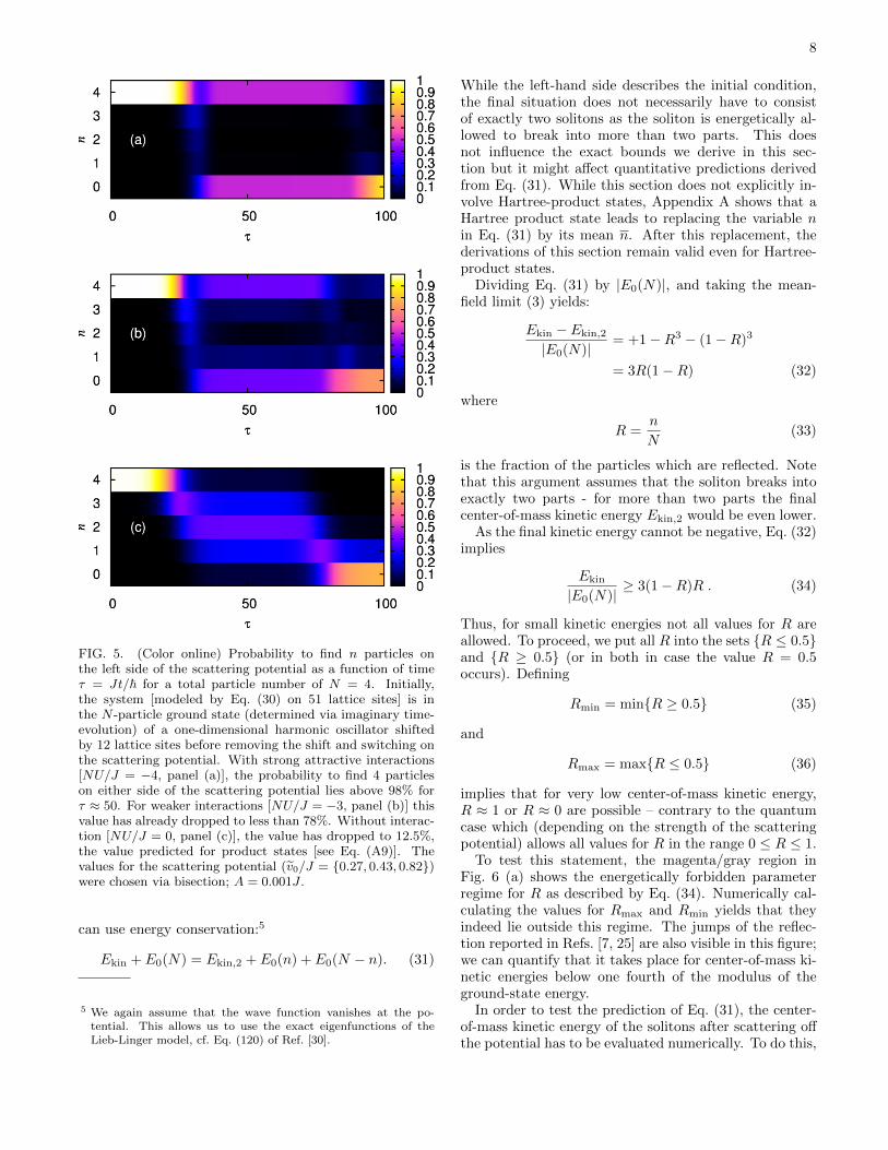
Figure 5 shows the difference between the regime ofperfect MQS like (11) in the regime of low center-of-masskinetic energy [Fig. 5 (a), cf. Sec. IV B] compared withthe high kinetic energy regime [Fig. 5 (c)] and the regimeof medium kinetic energies [Fig. 5 (b)]. In the high-energy regime, the final state corresponds to a productstate for which the probability distribution of particlenumbers always has a single peak. Bimodal distribu-tions correspond to quantum superpositions of (for smallparticle numbers) primarily two states, |n1, N − n1〉 and|n2, N−n2〉 for which the n1 and n2 differ by more than 1.

V. BOUNDS AND QUANTITATIVEPREDICTIONS FOR THE GPE-SOLUTIONS

Without the harmonic confinement, the qualitative be-havior is the same as in Sec. IV C; in addition, as soon asthe probability to find particles on the scattering poten-tial is small, the exact eigensolutions of the Lieb-Linigerequations are sufficient to expand the wave function.

Including center-of-mass kinetic energy and usingagain the notation that n particles are on one side andN − n on the other side of the scattering potential, we

8

FIG. 5. (Color online) Probability to find n particles onthe left side of the scattering potential as a function of timeτ = Jt/~ for a total particle number of N = 4. Initially,the system [modeled by Eq. (30) on 51 lattice sites] is inthe N -particle ground state (determined via imaginary time-evolution) of a one-dimensional harmonic oscillator shiftedby 12 lattice sites before removing the shift and switching onthe scattering potential. With strong attractive interactions[NU/J = −4, panel (a)], the probability to find 4 particleson either side of the scattering potential lies above 98% forτ ≈ 50. For weaker interactions [NU/J = −3, panel (b)] thisvalue has already dropped to less than 78%. Without interac-tion [NU/J = 0, panel (c)], the value has dropped to 12.5%,the value predicted for product states [see Eq. (A9)]. Thevalues for the scattering potential (v0/J = 0.27, 0.43, 0.82)were chosen via bisection; A = 0.001J .

can use energy conservation:5

Ekin + E0(N) = Ekin,2 + E0(n) + E0(N − n). (31)

5 We again assume that the wave function vanishes at the po-tential. This allows us to use the exact eigenfunctions of theLieb-Linger model, cf. Eq. (120) of Ref. [30].

While the left-hand side describes the initial condition,the final situation does not necessarily have to consistof exactly two solitons as the soliton is energetically al-lowed to break into more than two parts. This doesnot influence the exact bounds we derive in this sec-tion but it might affect quantitative predictions derivedfrom Eq. (31). While this section does not explicitly in-volve Hartree-product states, Appendix A shows that aHartree product state leads to replacing the variable nin Eq. (31) by its mean n. After this replacement, thederivations of this section remain valid even for Hartree-product states.

Dividing Eq. (31) by |E0(N)|, and taking the mean-field limit (3) yields:

Ekin − Ekin,2

|E0(N)| = +1−R3 − (1−R)3

= 3R(1−R) (32)

where

R =n

N(33)

is the fraction of the particles which are reflected. Notethat this argument assumes that the soliton breaks intoexactly two parts - for more than two parts the finalcenter-of-mass kinetic energy Ekin,2 would be even lower.

As the final kinetic energy cannot be negative, Eq. (32)implies

Ekin

|E0(N)| ≥ 3(1−R)R . (34)

Thus, for small kinetic energies not all values for R areallowed. To proceed, we put all R into the sets R ≤ 0.5and R ≥ 0.5 (or in both in case the value R = 0.5occurs). Defining

Rmin = minR ≥ 0.5 (35)

and

Rmax = maxR ≤ 0.5 (36)

implies that for very low center-of-mass kinetic energy,R ≈ 1 or R ≈ 0 are possible – contrary to the quantumcase which (depending on the strength of the scatteringpotential) allows all values for R in the range 0 ≤ R ≤ 1.

To test this statement, the magenta/gray region inFig. 6 (a) shows the energetically forbidden parameterregime for R as described by Eq. (34). Numerically cal-culating the values for Rmax and Rmin yields that theyindeed lie outside this regime. The jumps of the reflec-tion reported in Refs. [7, 25] are also visible in this figure;we can quantify that it takes place for center-of-mass ki-netic energies below one fourth of the modulus of theground-state energy.

In order to test the prediction of Eq. (31), the center-of-mass kinetic energy of the solitons after scattering offthe potential has to be evaluated numerically. To do this,

9

FIG. 6. Scattering a mean-field soliton off a delta potentialin a 1D situation without additional harmonic confinement.(a) The reflection Rmin (solid line) and Rmax (dotted line) asdefined in Eqs. (35) and (36) as a function of initial center-of-mass kinetic energy. As predicted by Eq. (34), both curves lieoutside the magenta/gray region for energetic reasons. (b)Scattering of a GPE soliton with initial center-of-mass ki-netic energy Ekin = 0.5|E0| as a function of the strengthof the delta-scattering potential, normalized such that with-out interaction, there would be 50:50 splitting [cf. Eq. (27)].From top to bottom: Dotted red/black line corresponds to thethe fraction psoliton of the final GPE-solution which is in soli-tons (the rest being particle-radiation). Solid magenta/grayline: Total kinetic energy after the scattering as predictedby Eq. (32) using the numerically calculated values for R.Dashed blue/black line: numerically calculated total kineticenergy. The difference between the two lower lines is onlylarge if psoliton < 1.

we perform a numerical scattering transform as describedin Ref. [55]. Figure 6 (b) demonstrates that Eq. (31)gives a good qualitative description of the final center-of-mass kinetic energy, but there is no perfect agreement.This can be explained by numerically calculating, againusing a numerical scattering transform, the fraction ofthe final wave function which is contained in solitons, therest being “radiation” of single particles having left thesoliton. Panel (b) also displays an interesting behaviornear the discontinuity of the reflection coefficient whichmanifests itself in a much better agreement of the twolower curves accompanied by nearly the whole GPE wavefunction being contained in solitons.

VI. CONCLUSION

We investigate scattering bright solitons generatedfrom potentials both on the mean-field level and on theN -particle quantum level in 1D. Adding an additionalharmonic confinement leads to interesting effects both onthe N -particle quantum level and on the GPE mean-fieldlevel:

Firstly, adding a harmonic confinement to the cre-ation of quantum superpositions of slow bright quantummatter-wave solitons provides a possibility to distinguishquantum superpositions from statistical mixtures: afterscattering off the potential twice, the probability that allparticles are on the side of the potential opposite to theinitial condition clearly distinguishes the two cases. Ason the single-particle level, changing the strength of thepotential leads to a continuously varying reflection (ortransmission) coefficient.

Secondly, for the reflection behavior of Gross-Pitaevskii solitons, we have derived analytic bounds onthe size of the jump of the reflection coefficient and de-rived the energy scale on which the step vanishes contin-uously for increasing center-of-mass kinetic energy. Thisbridges the two types of behavior previously reportedin the literature: bright solitons on the Gross-Pitaevskiilevel have been reported to split for larger energies (cf.[23, 24]) and display a stepwise reflection-behavior forlower center-of-mass kinetic energies [7, 25] for which theGPE-soliton hardly splits.

While the nonlinear character of the GPE does not al-low GPE-solutions which are quantum superpositions, weconjecture that the jumps in the transmission behaviorof the GPE-reflection coefficient indicates the formationof interesting quantum superpositions at the N-particlequantum level.

Note added: the jumps on the GPE-level were re-cently also investigated in Ref. [56].

ACKNOWLEDGMENTS

We thank Y. Castin, S. A. Gardiner, J. L. Helm,D. I. H. Holdaway, M. Holthaus, C. Lammerzahl andE. Zaremba for discussions. C.W. thanks R. G. Huletfor discussing the experiment [26]. We thank the Stu-dienstiftung des deutschen Volkes (B.G.) and the HeinzNeumuller Stiftung (B.G.), Durham University (T.B.)and the UK EPSRC (Grant No. EP/G05 6781/1, T.B.and C.W.) for funding. Computer power was obtainedfrom the GOLEM and HERO cluster of the Universityof Oldenburg and the cluster Hamilton at Durham Uni-versity. B.G. thanks C. S. Adams and S. A. Gardiner forthe hospitality during her visits at Durham University.

10

Appendix A: Re-deriving the bounds of Sec. V forHartree-product states in the limit N →∞

This section deals with Hartree-product states (10) forwhich the single-particle wave function ϕ(x, t∗) is zeronear the scattering potential and non-zero on both sidesof the scattering potential at a certain point of time t∗.Using properties of the eigenfunctions of the Lieb-Linigermodel [30] (Sec. A 1), we extend the calculations of Sec. Vto Hartree-product states. While this could, in princi-ple, lead to different results, in the limit N → ∞ werecover the same bounds as before (Sec. A 2). Onlyby assuming that the higher energy states not accessi-ble on the N -particle quantum level are also inaccessibleto Hartree-product states (cf. the footnote on page 3),Hartree-product states would predict a different reflec-tion behavior than observed at the GPE-level (Sec. A 3).

1. Justification why the eigenfunctions of theLieb-Liniger Model can be used

We take the scattering potential to have the form

Vscatt(x) = 0 for |x| > ζ , (A1)

which is fulfilled exactly for the delta function used inthis paper and approximately for Gaussian or 1/ cosh2(x)potentials.

The single-particle wave function defining the Hartree-product states (10) is assumed to fulfill:

0 =

∫ ζ

−ζ|ϕ(x, t∗)|2dx . (A2)

This requirement was fulfilled in the numerics of Sec. V;in the following we use that

p ≡∫ ∞ζ

|ϕ(x, t∗)|2dx (A3)

implies ∫ −ζ−∞|ϕ(x, t∗)|2dx = 1− p . (A4)

Equation (A2) implies that we can use the eigenfunc-tions of the Lieb-Liniger model to expand the wave-function. If n particles are on one side, they can forman n-particle soliton with energy:

〈E〉 = 〈Ekin〉+ E0(n) (A5)

where E0 is given by Eq. (8). Alternatively, it couldform several solitons or even free particles. However, anysuch combination has a higher energy E0 as E0(n+ n) ≤E0(n) + E0(n).

Thus, if n particles are on one side of the scatteringpotential and N − n on the other (which we denote by|n,N − n〉) and using the fact that the kinetic energy isnon-negative, we have:

〈n,N − n|H|n,N − n〉 ≥ E0(n) + E0(N − n) (A6)

2. Bounds on the energy in the limit N →∞

Using the notation introduced in Eq. (11), we can writethe total Hartree-product wave function at time t∗ as:

|ψ(x, t∗)〉 =

N∑n=0

cn|n,N − n〉, (A7)

which yields:

〈ψ(x, t∗)|H|ψ(x, t∗)〉 =

N∑n=0

|cn|2〈n,N − n|H|n,N − n〉 .

(A8)For Hartree-product states, the |cn|2 are given by theBinomial distribution [57, 3.2.2]:

|cn|2 =

(N

n

)pn(1− p)N−n, (A9)

where p is given by Eq. (A3). This distribution is stronglypeaked around

n = Np (A10)

with root-mean-square deviation

σ =√Np(1− p) . (A11)

Using Eq. (A6) we thus have:

〈ψ(x, t∗)|H|ψ(x, t∗)〉 ' 〈n,N − n|H|n,N − n〉≥ E0(n) + E0(N − n) ; (A12)

the larger N , the better the approximation in the firstline of Eq. (A12) becomes. By replacing Eq. (33) with

R =n

N(A13)

(which is the same as p), the equations and bound derivedin Sec. V are also valid for Hartree-product states. Forthe relation of the initial center-of-mass energy and thereflection coefficient we thus reproduce the equation (34):

Ekin

|E0(N)| ≥ 3(1−R)R . (A14)

This leads again to the statement that the magenta/grayregion of Fig. 6 is forbidden energetically.

3. Possible differences between Hartree-productstates and GPE: energy fluctuations

The above calculation did, however, use the limit N →∞ for which the distribution (A9) is very narrow. Forfinite N and low initial center-of-mass kinetic energy [cf.Eq. (A14)], energetically disallowed eigenfunctions likethose corresponding to |N/2, N/2〉 would always be an

11

important contribution to the sum (A7). The only way toprevent this (cf. footnote on page 3) is to predict that allparticles have to be on one side of the scattering potential(i.e., R = 0 or R = 1).

Hartree-product states for low particle numbers wouldthus behave differently from the GPE, which is strictlyspeaking only valid in the limit (3). Note thatthe contribution of energetically disallowed states like|N/2, N/2〉 vanishes only in the limit N → ∞ for whichlimN→∞ |cN/2/cn| = 0 (if N/2 6= n), although taking thislimit first and then apply energy arguments might be a

physically relevant approach.Thus, by extending this energy argument to higher

particle numbers one could construct an example forwhich a Hartree-product state disagrees in its “digital”prediction for the reflection coefficient with the GPE.This would, however, not confute the GPE. The fact thatHartree-product states are often used to derive the GPE(cf. [4]) does not necessarily imply that both always areequivalent; in general, the solutions of the GPE can al-ways be interpreted as |ϕ(x, t)|2 being the single-particledensity [29] rather than automatically being part of theHartree-product state (10).

[1] L. Khaykovich, F. Schreck, G. Ferrari, T. Bourdel, J. Cu-bizolles, L. D. Carr, Y. Castin, and C. Salomon, Science296, 1290 (2002)

[2] K. E. Strecker, G. B. Partridge, A. G. Truscott, and R. G.Hulet, Nature (London) 417, 150 (2002)

[3] S. L. Cornish, S. T. Thompson, and C. E. Wieman, Phys.Rev. Lett. 96, 170401 (2006)

[4] C. J. Pethick and H. Smith, Bose-Einstein Condensa-tion in Dilute Gases (Cambridge University Press, Cam-bridge, 2008)

[5] I. E. Mazets and G. Kurizki, Europhys. Lett. 76, 196(2006)

[6] C. Weiss and Y. Castin, Phys. Rev. Lett. 102, 010403(2009)

[7] A. I. Streltsov, O. E. Alon, and L. S. Cederbaum, Phys.Rev. A 80, 043616 (2009)

[8] L. D. Carr, C. W. Clark, and W. P. Reinhardt, Phys.Rev. A 62, 063611 (2000)

[9] U. Al Khawaja, H. T. C. Stoof, R. G. Hulet, K. E.Strecker, and G. B. Partridge, Phys. Rev. Lett. 89,200404 (2002)

[10] A. I. Streltsov, O. E. Alon, and L. S. Cederbaum, Phys.Rev. Lett. 106, 240401 (2011)

[11] L. Salasnich, A. Parola, and L. Reatto, Phys. Rev. A 66,043603 (2002)

[12] H. Buljan, M. Segev, and A. Vardi, Phys. Rev. Lett. 95,180401 (2005)

[13] L. Khaykovich and B. A. Malomed, Phys. Rev. A 74,023607 (2006)

[14] A. D. Martin, C. S. Adams, and S. A. Gardiner, Phys.Rev. Lett. 98, 020402 (2007)

[15] A. I. Streltsov, O. E. Alon, and L. S. Cederbaum, Phys.Rev. Lett. 100, 130401 (2008)

[16] H. Yanay, L. Khaykovich, and B. A. Malomed, Chaos 19,033145 (2009)

[17] S. Cornish, N. Parker, A. Martin, T. Judd, R. Scott,T. Fromhold, and C. Adams, Physica D: Nonlinear Phe-nomena 238, 1299 (2009)

[18] Y. S. Kivshar, S. A. Gredeskul, A. Sanchez, andL. Vazquez, Phys. Rev. Lett. 64, 1693 (1990)

[19] C. Muller, Appl. Phys. B-Lasers O 102, 459 (2011)[20] U. A. Khawaja, J. Phys. A 42, 265206 (2009)[21] T. Ernst and J. Brand, Phys. Rev. A 81, 033614 (2010)[22] T. P. Billam, S. L. Cornish, and S. A. Gardiner, Phys.

Rev. A 83, 041602(R) (2011)

[23] A. D. Martin and J. Ruostekoski, New J. Phys. 14,043040 (2012)

[24] J. L. Helm, T. P. Billam, and S. A. Gardiner, Phys. Rev.A 85, 053621 (2012)

[25] C. Lee and J. Brand, Europhys. Lett. 73, 321 (2006)[26] R. G. Hulet, private communicationS. E.

Pollack, D. Dries, E. J. Olson, and R. G.Hulet, 2010 DAMOP: Conference abstract,http://meetings.aps.org/link/BAPS.2010.DAMOP.R4.1

[27] E. H. Lieb and W. Liniger, Phys. Rev. 130, 1605 (1963)[28] J. B. McGuire, J. Math. Phys. 5, 622 (1964)[29] E. H. Lieb, R. Seiringer, and J. Yngvason, Phys. Rev. A

61, 043602 (2000)[30] Y. Castin and C. Herzog, C. R. Acad. Sci. Paris, Ser. 4

2, 419 (2001)[31] F. Calogero and A. Degasperis, Phys. Rev. A 11, 265

(1975)[32] Y. Castin and J. Dalibard, Phys. Rev. A 55, 4330 (1997)[33] J. Ruostekoski, M. J. Collett, R. Graham, and D. F.

Walls, Phys. Rev. A 57, 511 (1998)[34] J. A. Dunningham and K. Burnett, J. Mod. Opt. 48,

1837 (2001)[35] A. Micheli, D. Jaksch, J. I. Cirac, and P. Zoller, Phys.

Rev. A 67, 013607 (2003)[36] K. W. Mahmud, H. Perry, and W. P. Reinhardt, Phys.

Rev. A 71, 023615 (2005)[37] D. R. Dounas-Frazer, A. M. Hermundstad, and L. D.

Carr, Phys. Rev. Lett. 99, 200402 (2007)[38] D. Dagnino, N. Barberan, M. Lewenstein, and J. Dal-

ibard, Nature Phys. 5, 431 (2009)[39] B. Gertjerenken, S. Arlinghaus, N. Teichmann, and

C. Weiss, Phys. Rev. A 82, 023620 (2010)[40] M. A. Garcıa-March, D. R. Dounas-Frazer, and L. D.

Carr, Phys. Rev. A 83, 043612 (2011)[41] G. Mazzarella, L. Salasnich, A. Parola, and F. Toigo,

Phys. Rev. A 83, 053607 (2011)[42] L. Dell’Anna, Phys. Rev. A 85, 053608 (2012)[43] J. Holmer, J. Marzuola, and M. Zworski, J. Nonlinear

Sci. 17, 349 (2007)[44] D. I. H. Holdaway, C. Weiss, and S. A. Gardiner, Phys.

Rev. A 85, 053618 (2012)[45] K. Sacha, C. A. Muller, D. Delande, and J. Zakrzewski,

Phys. Rev. Lett. 103, 210402 (2009)[46] C. Weiss and Y. Castin, ArXiv e-prints(2012),

arXiv:1207.7131[47] Y. Castin, Eur. Phys. J. B 68, 317 (2009)

12

[48] C. Gross, private communication[49] S. Flugge, Rechenmethoden der Quantentheorie

(Springer, Berlin, 1990)[50] S. Dimopoulos, P. W. Graham, J. M. Hogan, and M. A.

Kasevich, Phys. Rev. Lett. 98, 111102 (2007)[51] C. Gross, T. Zibold, E. Nicklas, J. Esteve, and M. K.

Oberthaler, Nature (London) 464, 1165 (2010)[52] O. S. Sørensen, S. Gammelmark, and K. Mølmer, Phys.

Rev. A 85, 043617 (2012)[53] J. A. Glick and L. D. Carr, ArXiv e-prints(2011),

arXiv:1105.5164 [cond-mat.quant-gas]

[54] L. F. Shampine and M. K. Gordon, Computer Solutionof Ordinary Differential Equations (Freeman, San Fran-cisco, 1975)

[55] G. Boffetta and A. R. Osborne, J. Comp. Phys. 102, 252(1992)

[56] C.-H. Wang, T.-M. Hong, R.-K. Lee, and D.-W. Wang,ArXiv e-prints(2012), arXiv:1206.1606 [cond-mat.quant-gas]

[57] S. Haroche and J.-M. Raimond, Exploring the Quantum– Atoms, Cavities and Photons (Oxford University Press,Oxford, 2006)