Scaling of large-scale quantities in Rayleigh-Bénard ...home.iitk.ac.in/~mkv/Site/Publications_files/2016_Pandey_POF.pdf · Study of thermal convection is fundamental for the understanding

PHYSICS OF FLUIDS 28, 095105 (2016)

Scaling of large-scale quantities in Rayleigh-Bénardconvection

Ambrish Pandeya) and Mahendra K. Vermab)

Department of Physics, Indian Institute of Technology, Kanpur 208016, India

(Received 13 May 2016; accepted 22 August 2016; published online 16 September 2016)

We derive a formula for the Péclet number (Pe) by estimating the relative strengthsof various terms of the momentum equation. Using direct numerical simulationsin three dimensions, we show that in the turbulent regime, the fluid accelerationis dominated by the pressure gradient, with relatively small contributions arisingfrom the buoyancy and the viscous term; in the viscous regime, acceleration is verysmall due to a balance between the buoyancy and the viscous term. Our formulafor Pe describes the past experiments and numerical data quite well. We also showthat the ratio of the nonlinear term and the viscous term is ReRa−0.14, where Reand Ra are Reynolds and Rayleigh numbers, respectively, and that the viscousdissipation rate ϵu = (U3/d)Ra−0.21, where U is the root mean square velocity andd is the distance between the two horizontal plates. The aforementioned decrease innonlinearity compared to free turbulence arises due to the wall effects. Published byAIP Publishing. [http://dx.doi.org/10.1063/1.4962307]

I. INTRODUCTION

Study of thermal convection is fundamental for the understanding of heat transport in manynatural phenomena, e.g., in stars, Earth’s mantle, and atmospheric circulation. Many researchersstudy Rayleigh-Bénard convection (RBC), a simplified model of convection, in which a fluid keptbetween two horizontal plates at a distance d is heated from the bottom and cooled from thetop.1–6 Properties of the convective flow are primarily governed by two nondimensional parameters:the Prandtl number (Pr), a ratio of the kinematic viscosity ν and the thermal diffusivity κ, andthe Rayleigh number (Ra), a ratio of the buoyancy and the viscous forces. Two important globalquantities of RBC are the large-scale velocity U or a dimensionless Péclet number Pe = Ud/κ, andthe Nusselt number Nu, which is a ratio of the total and conductive heat transport; their dependenceon Ra and Pr has been studied extensively.1–4 In this paper, we derive an analytical formula forthe Péclet number that can explain the experimental and numerical results quite well. The formula,however, involves certain coefficients that are determined using numerical simulations. In additionto Pe, we also discuss the scaling of Nusselt number and dissipation rates.

Many researchers3,7–18 have studied the Nusselt and Reynolds numbers. Using the argumentsof marginal stability theory, Malkus7,8 deduced that Nu ≈ (Ra/Rac)1/3 by assuming that the heattransport is independent of d. Using mixing length theory, Kraichnan9 proposed that for very largeRayleigh numbers, the heat transport is independent of kinematic viscosity and thermal diffusivityof the fluid. The boundary layers in this “ultimate regime” become turbulent leading to Nu ∼

√RaPr

and Re ∼√

Ra/Pr.Castaing et al.10 performed experiments with helium gas (Pr ≈ 0.7) and observed Nu ∼ Ra0.28

and a Reynolds number Re = Pe/Pr ∼ Ra0.49 based on the peak frequency of the power spectrum.Sano et al.19 measured a Péclet number based on the mean vertical velocity near the side-wall

a)Electronic mail: [email protected])Electronic mail: [email protected]

1070-6631/2016/28(9)/095105/21/$30.00 28, 095105-1 Published by AIP Publishing.

Reuse of AIP Publishing content is subject to the terms at: https://publishing.aip.org/authors/rights-and-permissions. Downloaded to IP:

115.248.114.51 On: Fri, 16 Sep 2016 13:06:40

095105-2 A. Pandey and M. K. Verma Phys. Fluids 28, 095105 (2016)

and found that Pe ∼ Ra0.48. Castaing et al.10 proposed existence of a mixing zone where hotrising plumes meet mildly warm fluid. By matching the velocity of the hot fluid at the endof the mixing zone with those of the central region, Castaing et al.10 argued that Nu ∼ Ra2/7

and Rec ∼ Ra3/7, where Rec is based on the typical velocity scale in the central region. Usingthe properties of the boundary layer, Shraiman and Siggia11 derived that Nu ∼ Pr−1/7Ra2/7 andRe ∼ Pr−5/7Ra3/7[2.5 ln(Re) + 5]. They also derived exact relations between the Nusselt number andthe global viscous (ϵu) and thermal (ϵT) dissipation rates.3

One of the most recent and popular models of large-scale quantities of RBC is by Grossmannand Lohse13–17 (henceforth referred to as GL theory). In the exact relations of Shraiman and Siggia11

connecting the dissipation rates with the Nusselt and Reynolds numbers, Grossmann and Lohse13,14

substituted the contributions from the bulk and the boundary layers. This process enabled Gross-mann and Lohse to derive different formulae for the Nusselt and Reynolds numbers in the bulkand boundary-layer dominated regimes. The coefficients of the formulae were determined usingexperimental and simulation inputs. Later Stevens et al.18 updated the coefficients by includingmore recent simulation and experimental data. GL theory has been quite successful in explainingthe heat transport and Reynolds number in many numerical simulations and experiments. In thispaper, we derive a formula for the Péclet number using a different approach; we will contrast thedifferences between our model and GL towards the end of the paper.

The Reynolds number has been measured in many experiments and direct numerical simula-tions (DNSs) for a vast range of Rayleigh and Prandtl numbers, and it can be quantified in variousways: based on the maximum velocity of the horizontal velocity profiles,20,21 the absolute peakvalue of the vertical velocity,22,23 the root mean square (rms) velocity,21,24–26 etc. It can also becomputed using the peak frequency in power spectra of the temperature or velocity cross-correlationfunctions.12,21,27,28 Based on these estimates, Cioni et al.12 reported that Re ∼ Ra0.42 for mercury(Pr ≈ 0.022), and Qiu and Tong27 reported that Re ∼ Ra0.46 for water (Pr ≈ 5.4). Lam et al.21 stud-ied the Nusselt and Reynolds number scaling using experiments with organic fluids and measuredRe based on the oscillation frequency in large-scale flow. They showed that Re ∼ Ra0.43Pr−0.76 for3 ≤ Pr ≤ 1205 and 108 ≤ Ra ≤ 3 × 1010. Based on the volume-averaged rms velocity in numericalsimulations, Verma et al.24 observed that Pe scales as Ra0.43 and Ra0.49, respectively, for Pr = 0.2and 6.8, and Scheel and Schumacher25 found Re ∼ Ra0.49 for Pr = 0.7. In DNS of very large Prandtlnumbers, Silano et al.,22 Horn et al.,23 and Pandey et al.26 observed that Re ∼ Ra0.60.

In many experimental and numerical investigations,1–4,9,10,12–18,22–26,29–44 the Nusselt numberscales as Nu ∼ Raγ, where γ has been observed from 0.25 to 0.50. The exponent of 0.50 hasbeen reported for numerical experiments with periodic boundary condition24,35 and in turbulent freeconvection due to density gradient.45 A possible transition to the ultimate regime has been reportedin some experiments,30,36,43,44,46,47 while some others did not find any signature of a transition tothe ultimate regime.33,34,48–50 The Prandtl number dependence of the heat transport has also beeninvestigated in simulations32,41 and experiments.38,51 Verzicco and Camussi32 found Nu ∼ Pr0.14 forPr ≤ 0.35 and no variation beyond Pr = 0.35. Xia et al.38 observed that the heat transport decreasesweakly with the increase of Pr yielding Nu ∼ Ra0.30Pr−0.03 for 4 ≤ Pr ≤ 1353.

In RBC, the thermal plates induce anisotropy and sharp gradients in the flow. For example,the maximum drop in the temperature occurs mostly near the top and bottom plates, whereasthe temperature remains an approximate constant in the central region.39 Similarly, Emran andSchumacher52,53 and Stevens et al.40 reported that the thermal and the viscous dissipation ratesin the boundary layers exceed those in the bulk. In this paper, we compute the volume-averagedviscous and thermal dissipation rates and show that RBC has a lower nonlinearity compared tohomogeneous and isotropic flows of free or unbounded turbulence.

In this paper, we quantify various terms in the momentum equation and obtain an analyt-ical relation for Pe(Ra,Pr). The formula depends on certain coefficients that are determined usingnumerical simulations. Our derivation of Pe, which is very different from that of Grossman andLohse,13,14 has a single formula for Pe. We show in this paper that the predictions of our formulamatch with most of the experimental and numerical simulations. In this paper, we also discuss thePr and Ra dependence of the Nusselt number and the dissipation rates in RBC. Our analysis alsoshows that in the turbulent regime, the acceleration of a fluid parcel is dominated by the pressure

Reuse of AIP Publishing content is subject to the terms at: https://publishing.aip.org/authors/rights-and-permissions. Downloaded to IP:

115.248.114.51 On: Fri, 16 Sep 2016 13:06:40

095105-3 A. Pandey and M. K. Verma Phys. Fluids 28, 095105 (2016)

gradient. However in the viscous regime, the most dominant terms, the buoyancy and the viscousforce, balance each other.

The outline of the paper is the following. Section II contains the details about the governingequations. In Sec. III, we discuss the properties of the average temperature profile in RBC. InSec. IV, we construct a model to compute Pe as a function of Ra and Pr. Simulation details andcomparison of our model predictions with earlier results are discussed in Sec. V, and the scalingof Nusselt number and normalized thermal and viscous dissipation rates are presented in Sec. VI.Section VII contains the results of RBC simulations with free-slip boundary condition. We concludein Sec. VIII.

II. GOVERNING EQUATIONS

The equations of Rayleigh-Bénard convection under the Boussinesq approximation for a fluidconfined between two plates separated by a distance d are

∂u∂t+ (u · ∇)u = −∇σ

ρ0+ αgθz + ν∇2u, (1)

∂θ

∂t+ (u · ∇)θ = ∆

duz + κ∇2θ, (2)

∇ · u = 0, (3)

where u = (ux,uy,uz) is the velocity field, θ and σ are the deviations of temperature and pressurefrom the conduction state, ρ0,α, κ, and ν are, respectively, the mean density, the heat expansioncoefficient, the thermal diffusivity, and the kinematic viscosity of the fluid, ∆ is the temperaturedifference between top and bottom plates, g is the gravitational acceleration, and z is the unit vectorin the upward direction.

The two nondimensional parameters of RBC are the Rayleigh number Ra = αg∆d3/νκ andthe Prandtl number Pr = ν/κ. A nondimensionalized version of the above equations using d as thelength scale,

αg∆d as the velocity scale, ∆ as the temperature scale, and d/

αg∆d as the time

scale is

∂u′

∂t ′+ (u′ · ∇′)u′ = −∇′σ′ + θ ′z +

PrRa∇′2u′, (4)

∂θ ′

∂t ′+ (u′ · ∇′)θ ′ = u′z +

1√

RaPr∇′2θ ′, (5)

∇′ · u′ = 0. (6)

Here the primed variables represent dimensionless quantities. The magnitude of the large-scalevelocity is computed using the time-averaged total kinetic energy Eu as U =

2⟨Eu⟩t, where ⟨⟩t

denotes the averaging over time. The Péclet number is the ratio of the advection term and thediffusion term of the temperature equation, and it is defined as

Pe =|u · ∇θ ||κ∇2θ | =

Udκ

. (7)

Péclet number is analogous to Reynolds number, which is the ratio of the nonlinear term and theviscous term of the momentum equation.

In this paper, we study the rms values of the large-scale velocity and temperature fields, andother related global quantities like the Nusselt number and the dissipation rates.

III. TEMPERATURE PROFILE AND BOUNDARY LAYER

The temperature T(x, y, z) in a Rayleigh-Bénard cell fluctuates in time, and it can be decom-posed into a conductive profile and fluctuations superimposed on it, i.e.,

T(x, y, z) = Tc(z) + θ(x, y, z) = 1 − z + θ(x, y, z). (8)

Reuse of AIP Publishing content is subject to the terms at: https://publishing.aip.org/authors/rights-and-permissions. Downloaded to IP:

115.248.114.51 On: Fri, 16 Sep 2016 13:06:40

095105-4 A. Pandey and M. K. Verma Phys. Fluids 28, 095105 (2016)

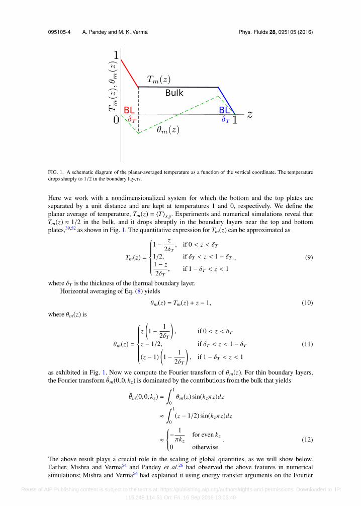
FIG. 1. A schematic diagram of the planar-averaged temperature as a function of the vertical coordinate. The temperaturedrops sharply to 1/2 in the boundary layers.

Here we work with a nondimensionalized system for which the bottom and the top plates areseparated by a unit distance and are kept at temperatures 1 and 0, respectively. We define theplanar average of temperature, Tm(z) = ⟨T⟩xy. Experiments and numerical simulations reveal thatTm(z) ≈ 1/2 in the bulk, and it drops abruptly in the boundary layers near the top and bottomplates,39,52 as shown in Fig. 1. The quantitative expression for Tm(z) can be approximated as

Tm(z) =

1 − z2δT

, if 0 < z < δT

1/2, if δT < z < 1 − δT1 − z2δT

, if 1 − δT < z < 1

, (9)

where δT is the thickness of the thermal boundary layer.Horizontal averaging of Eq. (8) yields

θm(z) = Tm(z) + z − 1, (10)

where θm(z) is

θm(z) =

z(1 − 1

2δT

), if 0 < z < δT

z − 1/2, if δT < z < 1 − δT

(z − 1)(1 − 1

2δT

), if 1 − δT < z < 1

(11)

as exhibited in Fig. 1. Now we compute the Fourier transform of θm(z). For thin boundary layers,the Fourier transform θm(0,0, kz) is dominated by the contributions from the bulk that yields

θm(0,0, kz) = 1

0θm(z) sin(kzπz)dz

≈ 1

0(z − 1/2) sin(kzπz)dz

≈

− 1πkz

for even kz

0 otherwise. (12)

The above result plays a crucial role in the scaling of global quantities, as we will show below.Earlier, Mishra and Verma54 and Pandey et al.26 had observed the above features in numericalsimulations; Mishra and Verma54 had explained it using energy transfer arguments on the Fourier

Reuse of AIP Publishing content is subject to the terms at: https://publishing.aip.org/authors/rights-and-permissions. Downloaded to IP:

115.248.114.51 On: Fri, 16 Sep 2016 13:06:40

095105-5 A. Pandey and M. K. Verma Phys. Fluids 28, 095105 (2016)

modes θ(2n,0,2n). A consequence of Eq. (12) is that the entropy spectrum

Eθ(k) =

k≤k′<k+1

12|θ(k′)|2 (13)

exhibits a dual branch—k−2 corresponding to Eq. (12) as the first branch, and a second branch forthe rest of the θ modes.26,54

It is interesting to note that the corresponding velocity mode, uz(0,0, kz) = 0 because of theincompressibility condition k · u(0,0, kz) = kzuz(0,0, kz) = 0. Also, ux(0,0, kz) = uy(0,0, kz) = 0 inthe absence of a mean flow along the horizontal direction. Hence for k = (0,0, kz) modes, themomentum equation yields

0 = − ikσ(k)ρ0

+ αgθ(k)z (14)

or dσm(z)/dz = ρ0αgθm. The dynamics of the remaining set of Fourier modes is governed by themomentum equation as

∂u(k)∂t+ i

p+q=k

[k · u(q)]u(p) = − ikσres(k)ρ0

+ αgθres(k)z − νk2u(k), (15)

where

θ = θres + θm, (16)σ = σres + σm. (17)

Hence, the modes θm(0,0, kz) and σm(0,0, kz) do not couple with the velocity modes in the mo-mentum equation, but θres and σres do.

In Sec. IV, we will quantify the large-scale velocity in RBC.

IV. UNIVERSAL FORMULA FOR U OR PÉCLET NUMBER

We derive an expression for the large-scale velocity U from the momentum equation [Eq. (1)].According to this equation, the material acceleration Du/Dt of a fluid element results from thepressure gradient, buoyancy, and the viscous force. Under steady state, we assume that ⟨∂u/∂t⟩ ≈ 0,hence, a dimensional analysis of the momentum equation yields

c1U2

d= c2

U2

d+ c3αgθres − c4ν

Ud2 , (18)

where ci’s are dimensionless coefficients. We observe in our numerical simulations (to be discussedlater) that the pressure gradient provides the acceleration to a fluid parcel whereas the viscous forceopposes the motion. Therefore we choose the sign of c2 same as that of c1, and the sign of c4 hasbeen chosen opposite to those of c1 and c2. In RBC, buoyancy provides additional acceleration;hence, c3 has the same sign as c1 and c2.

As discussed in Sec. III, the momentum equation contains θres = θ − θm, not θ. The coefficientsare defined as

c1 =|u · ∇u|U2/d

,

c2 =|∇σ |res/ρ0

U2/d,

c3 = |θres/∆|,c4 =

|∇2u|U/d2 . (19)

We will show later that ci’s are the functions of Ra and Pr that yields very interesting and nontrivialscaling relations. Note that typical dimensional arguments in fluid mechanics assume ci’s to beconstants, which is valid for free or unbounded turbulence.

Reuse of AIP Publishing content is subject to the terms at: https://publishing.aip.org/authors/rights-and-permissions. Downloaded to IP:

115.248.114.51 On: Fri, 16 Sep 2016 13:06:40

095105-6 A. Pandey and M. K. Verma Phys. Fluids 28, 095105 (2016)

Multiplication of Eq. (18) with d3/κ2 yields

c1Pe2 = c2Pe2 + c3RaPr − c4PePr, (20)

whose solution is

Pe =−c4Pr +

c2

4Pr2 + 4(c1 − c2)c3RaPr

2(c1 − c2) . (21)

Now we can compute the Péclet number using Eq. (21) given ci(Pr,Ra). We compute these coefficientsin Secs. V–VII. We remark that Pe could be a function of geometrical factors and aspect ratio.

In the viscous regime, the nonlinear term, u · ∇u, and the pressure gradient, −∇σ, are muchsmaller than the buoyancy and the viscous terms, hence in this regime

c3RaPr − c4PePr ≈ 0, (22)

which yields

Pe ≈ c3

c4Ra. (23)

We can deduce the properties under the turbulent regime by ignoring the viscous term in Eq. (20),which yields

c1Pe2 ≈ c2Pe2 + c3RaPr. (24)

The solution of the above equation is

Pe ≈

c3

|c1 − c2|RaPr. (25)

The above two limiting expressions of Pe can be derived from Eq. (21). We obtain turbulent regimewhen

Ra ≫c2

4Pr4c3|c1 − c2| (26)

and viscous regime for Ra ≪ c24Pr/(4c3|c1 − c2|). We will examine these cases once we deduce the

forms of ci’s using numerical simulations.In Sec. V, we compute the coefficients ci’s using our numerical simulation. Then we predict the

functional dependence of Pe(Ra,Pr).

V. NUMERICAL SIMULATION AND RESULTS

We perform RBC simulations by solving Eqs. (4)-(6) in a three-dimensional unit box forPr = 1,6.8, and 102 and Ra between 106 and 5 × 108 using an open-source finite-volume codeOF.55 We employ no-slip boundary condition for the velocity field at all the walls. For thetemperature field, we impose isothermal condition on the top and bottom plates, and adiabaticcondition at the vertical walls. The time stepping is performed using the second-order Crank-Nicolson method. Total number of grid points in our simulations vary from 603 to 2563 with finergrids employed near the boundary layers.56,57 We employ nonuniform mesh with higher concen-tration of grid points, from 4 to 6, near the boundaries. We validate our code by comparing theNusselt number with those computed in earlier numerical simulations and experiments. We showthat our results are grid-independent by showing that for Pr = 1 and Ra = 108, the Nusselt numbersfor 1003 and 2563 grids are close to each other within 3%. Figure 2 shows the temperature field ina vertical xz-plane at y = 0.4 for Pr = 1,6.8,102, and Ra = 5 × 107. Figures 2(b) and 2(c) exhibitmushroom-shaped sharper plumes, characteristics of a large Prandtl number RBC.2

Table I summarizes our simulation parameters, as well as the Péclet and Nusselt numbers,and kmaxηθ. For most of our runs, kmaxηθ ≥ 1, where ηθ is the Batchelor scale. The Batchelorscale ηθ = (κ3/ϵu)1/4 is related to the Kolmogorov scale ηu as ηθ = ηuPr−3/4. For Pr ≥ 1, ηθ ≤ ηu,

Reuse of AIP Publishing content is subject to the terms at: https://publishing.aip.org/authors/rights-and-permissions. Downloaded to IP:

115.248.114.51 On: Fri, 16 Sep 2016 13:06:40

095105-7 A. Pandey and M. K. Verma Phys. Fluids 28, 095105 (2016)

FIG. 2. For the no-slip boundary condition, the instantaneous temperature field in a vertical cross section at y = 0.4 forRa= 5×107 and (a) Pr= 1, (b) Pr= 6.8, and (c) Pr= 102. The flow structures or plumes get sharper as Pr increases.

TABLE I. Details of our simulations with no-slip boundary condition: N 3 is the total number of grid points.

Pr Ra N 3 Nu Pe kmaxηθ Pr Ra N 3 Nu Pe kmaxηθ

1 1 × 106 603 8.0 146.1 3.8 6.8 5 × 106 603 13.1 413.6 1.41 2 × 106 603 10.0 211.3 3.0 6.8 1 × 107 803 16.2 608.6 1.51 5 × 106 603 13.4 340.3 2.3 6.8 2 × 107 803 20.3 903.2 1.21 1 × 107 803 16.3 485.4 2.4 6.8 5 × 107 803 27.7 1536 0.81 2 × 107 803 20.2 687.4 1.9 102 1 × 106 603 8.5 190.7 1.21 5 × 107 803 26.8 1103 1.5 102 2 × 106 603 11.2 278.2 0.91 1 × 108 1003 32.9 1554 1.4 102 5 × 106 603 14.5 500.0 0.71 1 × 108 2563 31.9 1537 3.5 102 1 × 107 803 17.1 704.2 0.71 5 × 108 2563 51.2 3408 2.1 102 2 × 107 803 20.7 1044 0.66.8 1 × 106 603 8.4 182.7 2.3 102 5 × 107 803 27.7 1826 0.46.8 2 × 106 603 9.9 252.8 1.9 . . . . . . . . . . . . . . . . . .

FIG. 3. For the no-slip boundary condition, the comparison of the rms values of u ·∇u, (−∇σ)res, αgθresz, and ν∇2u as afunction of Ra for (a) Pr= 1 and (b) Pr= 102. The shaded region of panel (a) corresponds to the turbulent regime, while allthe runs of Pr= 102 belong to the viscous regime.

and therefore, the mean grid spacing should be smaller than ηθ. We continue the simulation tillit reaches statistical steady state, and then we compute averages of the rms values of |u · ∇u|,|(−∇σ)res|, |αgθresz|, and |ν∇2u|. We compute these quantities by first taking a volume average overthe entire box and then taking a time average. We perform these computations for a wide range of Prand Ra and plot them as a function of Ra in Fig. 3 for Pr = 1 and Pr = 100. The Ra-dependence of|u · ∇u|, |(−∇σ)res|, |αgθresz|, and |ν∇2u| is listed in Table II.

We observe that for Pr = 1 and Ra near 108 [the shaded region of Fig. 3(a)], the nonlinear term(|u · ∇u|) and the pressure gradient (|∇σ |) are much larger than the viscous and the buoyancy terms.

Reuse of AIP Publishing content is subject to the terms at: https://publishing.aip.org/authors/rights-and-permissions. Downloaded to IP:

115.248.114.51 On: Fri, 16 Sep 2016 13:06:40

095105-8 A. Pandey and M. K. Verma Phys. Fluids 28, 095105 (2016)

TABLE II. Scaling of various terms of the momentum equation (scaled asκ2/d3) for the no-slip boundary condition. The errors in the exponents areapproximately 0.02.

Turbulent regime Viscous regime

|u ·∇u| Ra1.2 Ra1.3

|(−∇σ)res| Ra1.1 Ra1.3

|αgθres| Ra0.87 Ra0.82

|ν∇2u| Ra0.87 Ra0.82

FIG. 4. For the no-slip boundary condition, the relative strengths of the forces acting on a fluid parcel. In the turbulentregime, the acceleration u ·∇u is provided primarily by the pressure gradient. In the viscous regime, the buoyancy and theviscous force dominate the pressure gradient, and they balance each other.

TABLE III. Functional dependence of the coefficients ci’s on Ra and Prunder the no-slip boundary condition.

c1 1.5Ra0.10Pr−0.06 c3 0.75Ra−0.15Pr−0.05

c2 1.6Ra0.09Pr−0.08 c4 20Ra0.24Pr−0.08

It is evident from the fact that the Reynolds number for Ra = 5 × 107,108,5 × 108 is approximately1103, 1537, and 3408, respectively. In the other limit, for Pr = 100 [Fig. 3(b)], the viscous force andbuoyancy are always larger than the nonlinear term and the pressure gradient. We depict the forcebalance in Fig. 4. Our numerical results are consistent with the intuitive pictures of the turbulent andviscous flows.

Using the rms values of the above quantities, we deduce that the functional dependence ofci’s is of the form listed in Table III. Following the similar approach as by Lam et al.21 and Xiaet al.38 to determine the functional dependence of Re(Ra,Pr) and Nu(Ra,Pr), respectively, we firstdetermine the Ra dependence of ci’s for Pr = 1,6.8, and 102 and find that the scaling exponentsare nearly similar for these Prandtl numbers. Then we determine the Pr dependence of ci’s forRa = 2 × 107. Combining these results, we obtain the functional dependence of ci’s, which are listedin Table III; the errors in the exponents of ci’s are / 0.01, except for the c4 − Ra scaling wherethe error is approximately 0.1. We also obtain nearly the same prefactors and exponents by fittingthe coefficients with the least square method. Clearly, ci’s are the weak functions of Pr, but theirdependence on Ra is reasonably strong so as to affect the Pe scaling significantly. Please note thatthe exponents of ci − Ra scaling depend weakly on the Prandtl number. Therefore the exponents inTable III are chosen as the average exponent for all the Prandtl numbers. In Fig. 5, we plot ci’s as afunction of Pr for Ra = 2 × 107 that exhibits approximately constant values. In Fig. 6, we exhibit thevariation of ci’s with Ra for Pr = 1,6.8, and 102.

Reuse of AIP Publishing content is subject to the terms at: https://publishing.aip.org/authors/rights-and-permissions. Downloaded to IP:

115.248.114.51 On: Fri, 16 Sep 2016 13:06:40

095105-9 A. Pandey and M. K. Verma Phys. Fluids 28, 095105 (2016)

FIG. 5. For the no-slip boundary condition, the variation of ci’s with Pr for Ra= 2×107. All the coefficients decrease weaklywith the increase of the Prandtl number.

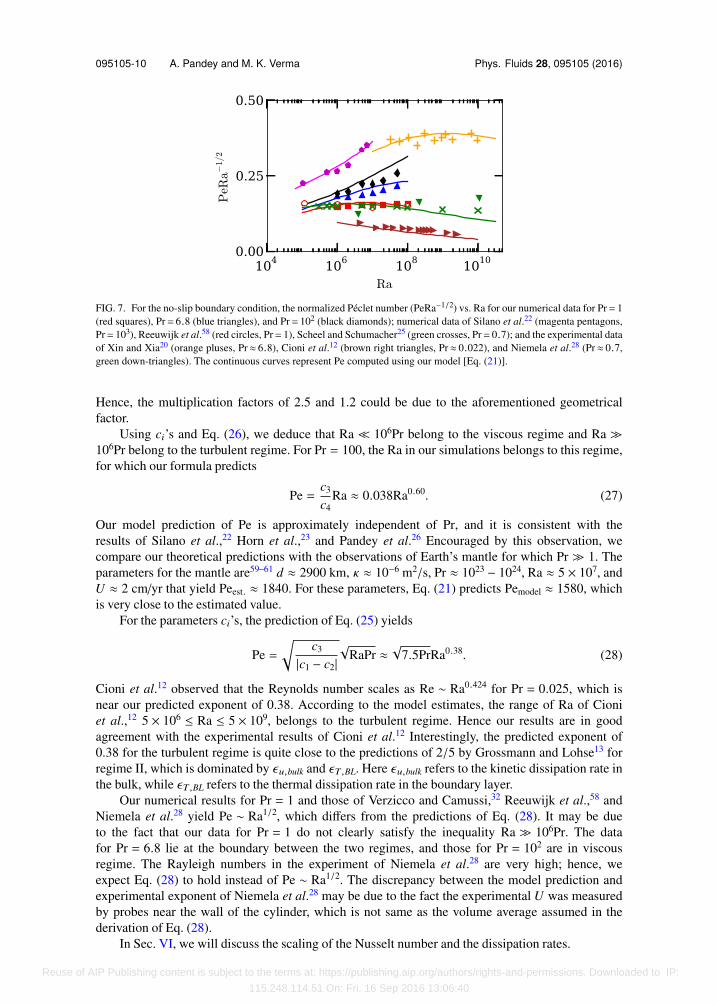
In Fig. 7, we plot the normalized Péclet number, PeRa−1/2, computed using our simulationdata for Pr = 1,6.8,102. The figure also contains the numerical results of Silano et al.22 (Pr = 103),Reeuwijk et al.58 (Pr = 1), Scheel and Schumacher25 (Pr = 0.7), and the experimental results ofXin and Xia20 (water, Pr ≈ 6.8), Cioni et al.12 (mercury, Pr ≈ 0.022), and Niemela et al.28 (helium,Pr ≈ 0.7). The continuous curves of Fig. 7 are the analytically computed Pe using Eq. (21) withthe coefficients ci’s listed in Table III. We observe that the theoretical predictions of Eq. (21) matchquite well with the numerical and experimental results, thus exhibiting usefulness of the model. Thepredictions of Eq. (21) for Pr = 0.022 and Pr = 6.8 have been multiplied with 2.5 and 1.2, respec-tively, to fit the experimental results from Cioni et al.12 and Xin and Xia.20 The correspondencebetween our predictions and the past experimental and numerical results shows that Pe is the func-tion of Pr and Ra, and it depends weakly on the geometrical factor and aspect ratio. Cioni et al.12

and Xin and Xia20 performed their experiments on cylinder, while our prediction is for a cube.

FIG. 6. For the no-slip boundary condition, the coefficients ci’s as a function of Ra. c1,c2, and c4 increase with increasingRa, whereas c3 decreases. The scaling exponents are nearly the same for all the Prandtl numbers. Legend applies to all theplots.

Reuse of AIP Publishing content is subject to the terms at: https://publishing.aip.org/authors/rights-and-permissions. Downloaded to IP:

115.248.114.51 On: Fri, 16 Sep 2016 13:06:40

095105-10 A. Pandey and M. K. Verma Phys. Fluids 28, 095105 (2016)

FIG. 7. For the no-slip boundary condition, the normalized Péclet number (PeRa−1/2) vs. Ra for our numerical data for Pr= 1(red squares), Pr= 6.8 (blue triangles), and Pr= 102 (black diamonds); numerical data of Silano et al.22 (magenta pentagons,Pr= 103), Reeuwijk et al.58 (red circles, Pr= 1), Scheel and Schumacher25 (green crosses, Pr= 0.7); and the experimental dataof Xin and Xia20 (orange pluses, Pr≈ 6.8), Cioni et al.12 (brown right triangles, Pr≈ 0.022), and Niemela et al.28 (Pr≈ 0.7,green down-triangles). The continuous curves represent Pe computed using our model [Eq. (21)].

Hence, the multiplication factors of 2.5 and 1.2 could be due to the aforementioned geometricalfactor.

Using ci’s and Eq. (26), we deduce that Ra ≪ 106Pr belong to the viscous regime and Ra ≫106Pr belong to the turbulent regime. For Pr = 100, the Ra in our simulations belongs to this regime,for which our formula predicts

Pe =c3

c4Ra ≈ 0.038Ra0.60. (27)

Our model prediction of Pe is approximately independent of Pr, and it is consistent with theresults of Silano et al.,22 Horn et al.,23 and Pandey et al.26 Encouraged by this observation, wecompare our theoretical predictions with the observations of Earth’s mantle for which Pr ≫ 1. Theparameters for the mantle are59–61 d ≈ 2900 km, κ ≈ 10−6 m2/s, Pr ≈ 1023 − 1024, Ra ≈ 5 × 107, andU ≈ 2 cm/yr that yield Peest. ≈ 1840. For these parameters, Eq. (21) predicts Pemodel ≈ 1580, whichis very close to the estimated value.

For the parameters ci’s, the prediction of Eq. (25) yields

Pe =

c3

|c1 − c2|√

RaPr ≈√

7.5PrRa0.38. (28)

Cioni et al.12 observed that the Reynolds number scales as Re ∼ Ra0.424 for Pr = 0.025, which isnear our predicted exponent of 0.38. According to the model estimates, the range of Ra of Cioniet al.,12 5 × 106 ≤ Ra ≤ 5 × 109, belongs to the turbulent regime. Hence our results are in goodagreement with the experimental results of Cioni et al.12 Interestingly, the predicted exponent of0.38 for the turbulent regime is quite close to the predictions of 2/5 by Grossmann and Lohse13 forregime II, which is dominated by ϵu,bulk and ϵT ,BL. Here ϵu,bulk refers to the kinetic dissipation rate inthe bulk, while ϵT ,BL refers to the thermal dissipation rate in the boundary layer.

Our numerical results for Pr = 1 and those of Verzicco and Camussi,32 Reeuwijk et al.,58 andNiemela et al.28 yield Pe ∼ Ra1/2, which differs from the predictions of Eq. (28). It may be dueto the fact that our data for Pr = 1 do not clearly satisfy the inequality Ra ≫ 106Pr. The datafor Pr = 6.8 lie at the boundary between the two regimes, and those for Pr = 102 are in viscousregime. The Rayleigh numbers in the experiment of Niemela et al.28 are very high; hence, weexpect Eq. (28) to hold instead of Pe ∼ Ra1/2. The discrepancy between the model prediction andexperimental exponent of Niemela et al.28 may be due to the fact the experimental U was measuredby probes near the wall of the cylinder, which is not same as the volume average assumed in thederivation of Eq. (28).

In Sec. VI, we will discuss the scaling of the Nusselt number and the dissipation rates.

Reuse of AIP Publishing content is subject to the terms at: https://publishing.aip.org/authors/rights-and-permissions. Downloaded to IP:

115.248.114.51 On: Fri, 16 Sep 2016 13:06:40

095105-11 A. Pandey and M. K. Verma Phys. Fluids 28, 095105 (2016)

VI. SCALING OF VISCOUS TERM, NUSSELT NUMBER, AND DISSIPATION RATES

The dependence of ci’s on Ra and Pr, which is due to the wall effects, affects the scaling ofother bulk quantities, e.g., dissipation rates and Nusselt number. We list some of the effects below.

A. Reynolds number revisited

For an unbounded or free turbulence, the ratio of the nonlinear term, u · ∇u, and the viscousterm is the Reynolds number Ud/ν. But this is not the case for RBC. The ratio

Nonlinear termViscous term

=|u · ∇u||ν∇2u| =

Udν

c1

c4∼ ReRa−0.14. (29)

Thus, for the same U,L, and ν, RBC has a weaker nonlinearity compared to the free or unboundedturbulence. This effect is purely due to the walls or the boundary layers.

B. Nusselt number scaling

In RBC, the flow is anisotropic due to the presence of buoyancy, which leads to a convectiveheat transport, quantified using Nusselt number,1,2,4 as

Nu =κ∆/d + ⟨uzθres⟩V

κ∆/d= 1 +

uzdκ

θres

∆

V

= 1 + Cuθres⟨u′2z ⟩1/2V ⟨θ′2res⟩1/2

V , (30)

where ⟨⟩V stands for a volume average, u′z = uzd/κ, θ ′res = θres/∆, and the normalized correlationfunction between the vertical velocity and the residual temperature fluctuation24 is

Cuθres =⟨u′zθ ′res⟩V

⟨u′2z ⟩1/2V ⟨θ′2res⟩1/2

V

. (31)

We compute the above quantities using the numerical data for various Ra and Pr. In Fig. 8, we plotthe normalized Nusselt number, NuRa−0.30, vs. Ra for our results, as well as earlier numerical22,40,42

and experimental results.12,20,38,62 The plot indicates that the Nusselt number exponent is close to0.30, and it is in good agreement with the earlier results for whom the exponents range from 0.27 to0.33.

The deviation of the exponent from 1/2 (ultimate regime9) is due to nontrivial correlation Cuθres

between uz and ⟨θres⟩. In Table IV, we list the scaling of Nu and Cuθres in the turbulent and viscous

FIG. 8. For the no-slip boundary condition, the normalized Nusselt number (NuRa−0.30) vs. Ra. Experimental data: Xiaet al.38 (Pr= 205, black pluses; Pr= 818, black left-pointing triangles), Cioni et al.12 (4 < Pr < 8.6, burlywood horizontalhexagons), Zhou et al.62 (5.2 < Pr < 7, blue stars), Xin and Xia20 (Pr≃ 7, blue circles). Numerical data: our data (Pr= 1,red squares; Pr= 6.8, blue triangles; Pr= 102, black diamonds), Silano et al.22 (Pr= 102, red crosses and Pr= 103, magentapentagons), Stevens et al.40 (Pr= 0.7, downward green triangles), and Scheel et al.42 (Pr= 0.7, pink vertical hexagons). Thedashed line represents Nu= 0.13Ra0.30.

Reuse of AIP Publishing content is subject to the terms at: https://publishing.aip.org/authors/rights-and-permissions. Downloaded to IP:

115.248.114.51 On: Fri, 16 Sep 2016 13:06:40

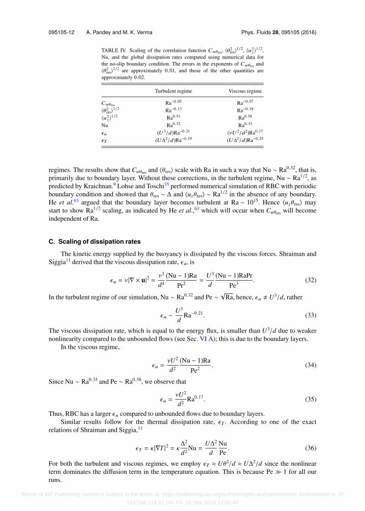
095105-12 A. Pandey and M. K. Verma Phys. Fluids 28, 095105 (2016)

TABLE IV. Scaling of the correlation function Cuθres, ⟨θ2res⟩1/2, ⟨u2

z⟩1/2,Nu, and the global dissipation rates computed using numerical data forthe no-slip boundary condition. The errors in the exponents of Cuθres and⟨θ2

res⟩1/2 are approximately 0.01, and those of the other quantities areapproximately 0.02.

Turbulent regime Viscous regime

Cuθres Ra−0.05 Ra−0.07

⟨θ2res⟩1/2 Ra−0.13 Ra−0.18

⟨u2z⟩1/2 Ra0.51 Ra0.58

Nu Ra0.32 Ra0.33

ϵu (U3/d)Ra−0.21 (νU2/d2)Ra0.17

ϵT (U∆2/d)Ra−0.19 (U∆2/d)Ra−0.25

regimes. The results show that Cuθres and ⟨θres⟩ scale with Ra in such a way that Nu ∼ Ra0.32, that is,primarily due to boundary layer. Without these corrections, in the turbulent regime, Nu ∼ Ra1/2, aspredicted by Kraichnan.9 Lohse and Toschi35 performed numerical simulation of RBC with periodicboundary condition and showed that θres ∼ ∆ and ⟨uzθres⟩ ∼ Ra1/2 in the absence of any boundary.He et al.63 argued that the boundary layer becomes turbulent at Ra ∼ 1015. Hence ⟨uzθres⟩ maystart to show Ra1/2 scaling, as indicated by He et al.,63 which will occur when Cuθres will becomeindependent of Ra.

C. Scaling of dissipation rates

The kinetic energy supplied by the buoyancy is dissipated by the viscous forces. Shraiman andSiggia11 derived that the viscous dissipation rate, ϵu, is

ϵu = ν |∇ × u|2 = ν3

d4

(Nu − 1)RaPr2 =

U3

d(Nu − 1)RaPr

Pe3 . (32)

In the turbulent regime of our simulation, Nu ∼ Ra0.32 and Pe ∼√

Ra, hence, ϵu , U3/d, rather

ϵu ∼U3

dRa−0.21. (33)

The viscous dissipation rate, which is equal to the energy flux, is smaller than U3/d due to weakernonlinearity compared to the unbounded flows (see Sec. VI A); this is due to the boundary layers.

In the viscous regime,

ϵu =νU2

d2

(Nu − 1)RaPe2 . (34)

Since Nu ∼ Ra0.33 and Pe ∼ Ra0.58, we observe that

ϵu =νU2

d2 Ra0.17. (35)

Thus, RBC has a larger ϵu compared to unbounded flows due to boundary layers.Similar results follow for the thermal dissipation rate, ϵT . According to one of the exact

relations of Shraiman and Siggia,11

ϵT = κ |∇T |2 = κ∆2

d2 Nu =U∆2

dNuPe

. (36)

For both the turbulent and viscous regimes, we employ ϵT ≈ Uθ2/d ≈ U∆2/d since the nonlinearterm dominates the diffusion term in the temperature equation. This is because Pe ≫ 1 for all ourruns.

Reuse of AIP Publishing content is subject to the terms at: https://publishing.aip.org/authors/rights-and-permissions. Downloaded to IP:

115.248.114.51 On: Fri, 16 Sep 2016 13:06:40

095105-13 A. Pandey and M. K. Verma Phys. Fluids 28, 095105 (2016)

Hence, substitution of the expressions for Pe and Nu in the above equation yields the followingϵT for the turbulent regime of our simulations:

ϵT ∼U∆2

dRa−0.19, (37)

but

ϵT ∼U∆2

dRa−0.25 (38)

for the viscous regime. The above Ra-dependent corrections are also due to the boundary layers. Inthe turbulent regime, for Pr = 1, the ratio of the nonlinear term of the temperature equation and thethermal diffusion term is

u · ∇θκ∇2θ

=c5

c6

Udκ∼ Ra−0.30Pe, (39)

since

c5 =|u · ∇θ |Uθ/d

∼ Ra0.09,

c6 =|∇2θ |θ/d2 ∼ Ra0.39. (40)

Thus, the nonlinearity in the temperature equation [Eq. (2)] of RBC is weaker than the correspond-ing term in unbounded flow (e.g., passive scalar in a periodic box). Consequently the entropy flux isweaker than that for unbounded flows, which is the reason for the behavior of Eqs. (37) and (38).

We numerically compute the following normalized dissipation rates:

Cϵu,1 =ϵu

U3/d=

(Nu − 1)RaPrPe3 ∼ Ra−0.21Pr (turbulent regime), (41)

Cϵu,2 =ϵu

νU2/d2 =(Nu − 1)Ra

Pe2 ∼ Ra0.17 (viscous regime), (42)

CϵT =ϵT

Uθ2/d=

NuPe∼ Ra−0.25, (43)

which are plotted in Fig. 9. We observe that Cϵu,1/Pr ∼ Ra−0.22±0.02 and Ra−0.25±0.03 for Pr = 1and 6.8, respectively, which are in good agreement with Eq. (41). The exponents for Cϵu,2 are0.22 ± 0.01 and 0.19 ± 0.02 for Pr = 6.8 and 102, respectively, with reasonable accordance withEq. (35) for Pr = 102. For the thermal dissipation rate, we observe CϵT ∼ Ra−0.32±0.02 scaling forPr = 1,6.8, and 102 consistent with the above scaling. Table IV lists the Ra-dependence of thedissipation rates in the turbulent and viscous regimes.

FIG. 9. The normalized dissipation rates for the no-slip boundary condition: (a)Cϵu,1/Pr, (b)Cϵu,2, and (c)CϵT as functionsof Ra for Pr= 1 (red squares), Pr= 6.8 (blue triangles), and Pr= 102 (black diamonds). The best fits to the data are depictedas solid lines.

Reuse of AIP Publishing content is subject to the terms at: https://publishing.aip.org/authors/rights-and-permissions. Downloaded to IP:

115.248.114.51 On: Fri, 16 Sep 2016 13:06:40

095105-14 A. Pandey and M. K. Verma Phys. Fluids 28, 095105 (2016)

We estimate the dissipation rate (product of the dissipation rate and the appropriate volume) inthe bulk, Du,bulk, and in the boundary layer, Du,BL. Their ratio is

Du,BL

Du,bulk≈

(ϵu,BL)(2Aδu)(ϵu,bulk)(Ad − 2Aδu) ≈

(2νU2/δ2

u

U3/d

)δud

≈ 2d/δuRe≈ 2Re−1/2 (44)

since δu/d ∼ Re−1/2.64 Here A is the area of the horizontal plates, and δu is the thickness of theviscous boundary layers at the top and bottom plates. Since the dissipation takes place near boththe plates, we include a factor 2 here. Note that we do not substitute the weak Ra dependence ofEqs. (33) and (35) as an approximation. From Eq. (44) we deduce that Du,BL ≪ Du,bulk for large Re.However in the viscous regime, the boundary layer extends to the whole region (2δu ≈ d); hence,Du,BL dominates Du,bulk.

Earlier, Grossmann and Lohse13–15 worked out the scaling of the Reynolds and Nusselt num-bers by invoking the exact relations of Shraiman and Siggia11 and using the fact that the totaldissipation is a sum of those in the bulk and in the boundary layers (Du,bulk and Du,BL, respec-tively). They employed ϵu,bulk = U3/d, ϵT ,bulk = U∆2/d, ϵu,BL = νU2/δ2

u, and ϵT ,BL = κ∆2/δ2T , and

then equated one of the expressions in the appropriate regimes. They also employed corrections forlarge Pr and small Pr cases. Our model discussed in this paper is an alternative to that of GL with anattempt to highlight the anisotropic effects arising due to the boundary layers that yield ϵu , U3/dand ϵT , U∆2/d. Note that we report a single formula for Pe in comparison to the eight expressionsof Grossman and Lohse13 for various limiting cases.

From the above derivation it is apparent that the boundary layers of RBC have significant ef-fects on the large-scale quantities; consequently the flow behavior in RBC is very different from theunbounded fluid turbulence for which we employ homogeneous and isotropic formalism. In partic-ular, for a free turbulence under the isotropy assumption, ⟨u′zθ ′res⟩V = 0, hence the nonzero Cuθres forRBC is purely due to the walls or boundary layers. To relate to the scaling in the ultimate regime, weconjecture that Cuθres, θ

′res, and ci’s would become independent of Ra due to the detachment of the

boundary layer, hence Nu ∼ ⟨u′2z ⟩1/2 ∼ Ra1/2, as predicted by Kraichnan.9 Note that for a nonzeroNu, Cuθres must be finite, contrary to the predictions for isotropic turbulence for which Cuθres = 0.We need further experimental inputs as well as numerical simulations at very large Ra to test theabove conjecture.

Here we end our discussion on RBC with the no-slip boundary condition. In Sec. VII, we willdiscuss the scaling relations for RBC with the free-slip boundary condition.

VII. RESULTS OF RBC WITH FREE-SLIP BOUNDARY CONDITION

In this section, we will study the scaling of Péclet number under free-slip boundary condition.Towards this objective we perform RBC simulations with free-slip walls for a set of Prandtl andRayleigh numbers and compute the strengths of the nonlinear term, pressure gradient, buoyancy,and the viscous force, and the corresponding coefficients ci’s defined in Sec. IV. After this wecompute the Péclet number as a function of Pr and Ra. The procedure is identical to that describedfor the no-slip boundary condition.

We perform direct numerical simulations for Pr = 0.02,1,4.38,102,103, and ∞, and Rayleighnumbers between 105 and 2 × 108 in a three-dimensional unit box using a pseudo-spectral codeT.65 For the velocity field, we employ free-slip boundary condition at all the walls, and for thetemperature field, the isothermal condition at the top and bottom plates, and the adiabatic conditionat the vertical walls. We use the fourth-order Runge-Kutta (RK4) method for time discretizationand 2/3 rule to dealiase the fields. We start our simulations for lower Ra using random initialvalues for the velocity and temperature fields and then take the steady-state fields as the initialcondition to simulate for higher Rayleigh numbers. We employ 643 to 5123 grids and ensure thatthe Kolmogorov (ηu) and the Batchelor (ηθ) lengths are larger than the mean distance between twoadjacent grid points for each simulation. The details of simulation parameters are given in Table V.

Reuse of AIP Publishing content is subject to the terms at: https://publishing.aip.org/authors/rights-and-permissions. Downloaded to IP:

115.248.114.51 On: Fri, 16 Sep 2016 13:06:40

095105-15 A. Pandey and M. K. Verma Phys. Fluids 28, 095105 (2016)

TABLE V. Details of our simulations with the stress-free boundary condition. The quantities are same as in Table I, exceptη is the Kolmogorov length scale (ηu) for Pr= 0.02.

Pr Ra N 3 Nu Pe kmaxη Pr Ra N 3 Nu Pe kmaxη

0.02 1 × 105 2563 4.93 4.02 × 101 4.6 102 1 × 106 1283 20.8 7.49 × 102 1.90.02 2 × 105 2563 5.74 5.28 × 101 3.7 102 2 × 106 2563 29.0 1.23 × 103 3.00.02 5 × 105 5123 7.21 7.71 × 101 5.4 102 5 × 106 2563 39.2 2.15 × 103 2.20.02 1 × 106 5123 8.65 1.01 × 102 4.3 102 1 × 107 2563 45.8 3.21 × 103 1.70.02 2 × 106 5123 10.7 1.41 × 102 3.4 102 2 × 107 2563 58.0 5.00 × 103 1.41 1 × 106 643 18.5 4.68 × 102 3.0 102 5 × 107 5123 77.4 8.70 × 103 2.01 2 × 106 643 21.9 6.07 × 102 2.5 103 1 × 106 2563 21.5 7.54 × 102 2.11 5 × 106 1283 28.4 8.84 × 102 3.7 103 2 × 106 2563 27.1 1.16 × 103 1.71 1 × 107 1283 32.6 1.16 × 103 3.0 103 5 × 106 2563 36.0 2.04 × 103 1.21 2 × 107 1283 39.5 1.57 × 103 2.4 103 1 × 107 5123 45.3 3.09 × 103 2.01 5 × 107 2563 49.1 2.36 × 103 3.6 103 2 × 107 5123 54.1 4.29 × 103 1.61 1 × 108 2563 60.1 3.11 × 103 2.9 103 5 × 107 5123 75.2 8.03 × 103 1.24.38 1 × 106 1283 21.5 6.98 × 102 4.1 103 1 × 108 5123 91.4 1.25 × 104 0.94.38 2 × 106 1283 26.4 9.65 × 102 1.6 ∞ 5 × 106 2563 35.3 2.03 × 103 7.04.38 5 × 106 1283 33.9 1.47 × 103 2.4 ∞ 1 × 107 2563 43.6 3.10 × 103 5.64.38 1 × 107 1283 41.0 1.96 × 103 1.9 ∞ 2 × 107 2563 54.4 4.46 × 103 4.54.38 2 × 107 2563 48.5 2.61 × 103 3.2 ∞ 5 × 107 2563 72.4 7.95 × 103 3.34.38 5 × 107 2563 62.3 3.88 × 103 2.4 ∞ 1 × 108 2563 92.3 1.33 × 104 2.6. . . . . . . . . . . . . . . . . . ∞ 2 × 108 5123 113 1.92 × 104 4.2

Figure 10 demonstrates the temperature field in a vertical cross section of the box at y = 0.4. Thetemperature field is diffusive for Pr = 0.02, whereas the field becomes plume-dominated for largerPrandtl numbers.2

We compute the rms values of |u · ∇u|, |(−∇σ)res|, |αgθresz|, and |ν∇2u| for Pr = 1 and 103.These values are plotted as a function of Ra in Fig. 11, and their Ra-dependence is given inTable VI. From the numerical data we can deduce the following:

1. In the turbulent regime (for Pr = 1 of Fig. 11(a)), the acceleration is dominated by the pressuregradient; the buoyancy and viscous terms are quite weak in comparison. This feature is sameas that for the no-slip boundary condition (see Sec. V). However, for the free-slip boundarycondition, both vertical and horizontal accelerations are significant (see Fig. 12(a)).

2. In the viscous regime (for Pr = 103 of Fig. 11(b)), the nonlinear term is weak, and (−∇σ)res,αgθresz, and ν∇2u balance each other as shown in Fig. 12(b). Interestingly the pressure gradientopposes the motion. We will revisit this issue in the following discussion. Note that for theno-slip boundary condition, the nonlinear term and the pressure gradient are weak (see Sec. V).

FIG. 10. For the free-slip boundary condition, the temperature field in a vertical plane at y = 0.4 for (a) Pr= 0.02,Ra= 2×106, (b) Pr= 1,Ra= 5×107, and (c) Pr= 102,Ra= 5×107. Thermal structures become sharper with increasing Prandtlnumber.

Reuse of AIP Publishing content is subject to the terms at: https://publishing.aip.org/authors/rights-and-permissions. Downloaded to IP:

115.248.114.51 On: Fri, 16 Sep 2016 13:06:40

095105-16 A. Pandey and M. K. Verma Phys. Fluids 28, 095105 (2016)

FIG. 11. For the free-slip boundary condition, comparison of the rms values of u ·∇u, (−∇σ)res, αgθresz, and ν∇2u as afunction of Ra (a) in the turbulent regime (Pr= 1) and (b) in viscous regime (Pr= 103).

TABLE VI. Rayleigh number dependence of various terms of the momen-tum equation (scaled as κ2/d3) for the free-slip boundary condition. Theerrors in the exponents are approximately 0.02.

Turbulent regime Viscous regime

|u ·∇u| Ra1.1 Ra1.3

|(−∇σ)res| Ra1.0 Ra0.86

|αgθres| Ra0.89 Ra0.86

|ν∇2u| Ra0.96 Ra0.89

FIG. 12. For the free-slip boundary condition, the relative strengths of the forces acting on a fluid parcel. In turbulent regime,the acceleration u ·∇u is provided primarily by the pressure gradient, both in parallel and perpendicular directions. In viscousregime, the buoyancy is balanced by the pressure gradient and the viscous force along z; in the perpendicular direction, thepressure gradient balances the viscous force.

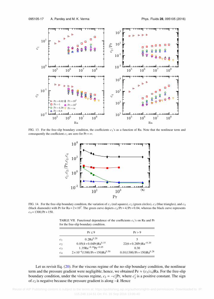
After the computation of each of the terms of the momentum equation, we compute the coef-ficients ci’s that have been defined in Sec. IV. The ci’s have been plotted in Fig. 13 as a functionof Ra, and in Fig. 14 as a function of Pr, and their functional form is tabulated in Table VII. Theci’s for the free-slip boundary condition differ in certain ways from those for the no-slip boundarycondition. For the viscous regime (here large Pr) of free-slip flows, −∇σ is significant. For theconsistency of Eq. (20), we require that c1 = 0 and c2 ∝ Pr in order to cancel Pr in the Pr → ∞regime. This is the reason we write c2 = −c′2Pr under the free-slip boundary condition. For verylarge Pr, the linear term of c2 dominates its constant counterpart. Note that for the no-slip boundarycondition in the viscous limit, −∇σ ≈ 0, and the viscous force and the buoyancy cancel each other.Hence, the no-slip and the free-slip boundary conditions yield different results.

Reuse of AIP Publishing content is subject to the terms at: https://publishing.aip.org/authors/rights-and-permissions. Downloaded to IP:

115.248.114.51 On: Fri, 16 Sep 2016 13:06:40

095105-17 A. Pandey and M. K. Verma Phys. Fluids 28, 095105 (2016)

FIG. 13. For the free-slip boundary condition, the coefficients ci’s as a function of Ra. Note that the nonlinear term andconsequently the coefficient c1 are zero for Pr=∞.

FIG. 14. For the free-slip boundary condition, the variation of c1 (red squares), c2 (green circles), c3 (blue triangles), and c4(black diamonds) with Pr for Ra= 2×107. The green curve depicts c2/Pr= 4/Pr+0.04, whereas the black curve representsc4= 1300/Pr+150.

TABLE VII. Functional dependence of the coefficients ci’s on Ra and Prfor the free-slip boundary condition.

Pr ≤ 9 Pr > 9

c1 0.2Ra0.20 5c2 0.05(4+0.04Pr)Ra0.15 22(6+0.28Pr)Ra−0.20

c3 1.35Ra−0.10Pr−0.05 0.30c4 2×10−4(1300/Pr+150)Ra0.50 0.01(1300/Pr+150)Ra0.28

Let us revisit Eq. (20). For the viscous regime of the no-slip boundary condition, the nonlinearterm and the pressure gradient were negligible; hence, we obtained Pe ≈ (c3/c4)Ra. For the free-slipboundary condition, under the viscous regime, c2 = −c′2Pr, where c′2 is a positive constant. The signof c2 is negative because the pressure gradient is along −z. Hence

Reuse of AIP Publishing content is subject to the terms at: https://publishing.aip.org/authors/rights-and-permissions. Downloaded to IP:

115.248.114.51 On: Fri, 16 Sep 2016 13:06:40

095105-18 A. Pandey and M. K. Verma Phys. Fluids 28, 095105 (2016)

FIG. 15. For the free-slip boundary condition, (a) the normalized Péclet number (PeRa−1/2) vs. Ra. The continuous curvesrepresent analytically computed Pe, which are approximately close to the numerical results. (b) The normalized Nusseltnumber (NuRa−0.30) as a function of Ra. For small and moderate Pr, Pe∼Ra0.45 and Nu∼Ra0.27, and for very large Prandtlnumbers, Pe∼Ra0.60 and Nu∼Ra0.32.

TABLE VIII. Summary of the scalings for free-slip boundary condition.Quantities are same as those in Table IV.

Turbulent regime Viscous regime

Cuθres Ra−0.06 Ra−0.17

⟨θ2res⟩1/2 Ra−0.10 Ra−0.12

⟨u2z⟩1/2 Ra0.43 Ra0.61

Nu Ra0.27 Ra0.32

ϵu U3/d (νU2/d2)Ra0.10

ϵT (U∆2/d)Ra−0.15 (U∆2/d)Ra−0.29

c′2Pe2 + c4Pe − c3Ra = 0, (45)

which yields

Pe =−c4 +

c2

4 + 4c′2c3Ra

2c′2. (46)

Note that the above Pe is independent of Pr as observed in numerical simulations.26 In the abovederivation, c2 ∝ Pr is an important ingredient.

In Fig. 15(a) we plot the normalized Péclet number PeRa−1/2 computed for various Pr. Here wealso plot the analytically computed Pe [Eq. (21)] with ci’s from Table VII as continuous curves. Weobserve that our formula fits quite well with the numerical results. In addition, we also compute Nu,θres, Cuθres, and dissipation rates. The functional dependence of these quantities with Ra is listed inTable VIII. Almost all the features are similar to those of the no-slip boundary condition except thatϵu ∝ U3/d, similar to unbounded flow, which may be due to weak viscous boundary layer for thefree-slip boundary condition. In Fig. 15(b) we plot the normalized Nusselt number computed for thefree-slip simulations. As can be observed from the figure, the Nusselt number increases with Prandtlnumber up to Pr = 102 and then it becomes approximately constant.

In summary, the scaling of large-scale quantities for the no-slip and free-slip boundary condi-tions has many similarities, but there are certain critical differences.

VIII. CONCLUSIONS

In this paper we derive a general formula for the Péclet number from the momentum equation.The general formula involves four coefficients that are determined using the numerical data. Thepredictions from our formula match with most of the past experimental and numerical results. Our

Reuse of AIP Publishing content is subject to the terms at: https://publishing.aip.org/authors/rights-and-permissions. Downloaded to IP:

115.248.114.51 On: Fri, 16 Sep 2016 13:06:40

095105-19 A. Pandey and M. K. Verma Phys. Fluids 28, 095105 (2016)

derivation is very different from that of Grossmann and Lohse13–15 who use the exact relations ofShraiman and Siggia.11 Also, GL’s formalism provides 8 different formulae for various limitingcases, but we provide a single formula, whose coefficients are determined using numerical data.

In our paper we also find several other interesting results, which are listed below:

1. In RBC, the planar average of temperature drops sharply near the boundary layers, and it re-mains approximately a constant in the bulk. A consequence of the above observation is that theFourier transform of the average temperature θm exhibits θm(0,0, kz) = −1/(πkz); hence, theentropy spectrum has a prominent branch Eθ(k) ∼ k−2. The above spectrum has been reportedearlier by Mishra and Verma54 and Pandey et al.26

2. The modes θm(0,0, kz) do not couple with the velocity modes in the momentum equation.Instead, the momentum equation involves θres = θ − θm. It has an important consequence on thescaling of the Péclet and Nusselt numbers.

3. The Nusselt number Nu = 1 + Cuθres⟨u2z⟩1/2

V ⟨θ2res⟩1/2

V . The Ra dependence of Cuθres, uz, and θres

yields corrections from the ultimate regime scaling Nu ∼ Ra1/2 to the experimentally realizedbehavior Nu ∼ Ra0.3.

4. For the no-slip boundary condition, we observe that

Nonlinear termViscous term

=|u · ∇u||ν∇2u| =

Udν

c1

c4∼ ReRa−0.14, (47)

where c1 ∼ Ra0.10 and c4 ∼ Ra0.24. Thus in RBC, the nonlinear term is weaker than that in freeturbulence. This is due to the wall effect. The numerical data also reveal that in the turbu-lent regime, the viscous dissipation rate or the Kolmogorov energy flux ϵu ∼ (U3/d)Ra−0.21,consistent with the suppression of nonlinearity in RBC. Similarly, the thermal dissipation rate,ϵT ∼ (U∆2/d)Ra−0.19.

5. In the viscous regime of RBC, ϵu ∼ (νU2/d2)Ra0.17, thus the viscous dissipation rate isenhanced compared to unbounded flow.

6. Under the free-slip boundary condition, the behavior remains roughly the same as the no-slipboundary condition. The three main differences between the free-slip and no-slip boundaryconditions are as follows:

(a) The pressure gradient plays an important role in the viscous regime under the free-slipboundary condition, unlike the no-slip case.

(b) For the free-slip boundary condition, the horizontal components of the pressure gradientand viscous terms are significant, contrary to the no-slip case.

(c) For the free-slip case, ϵu ∼ (U3/d) because of the weaker viscous boundary layer. How-ever for the no-slip case, ϵu ∼ (U3/d)Ra−0.21.

In summary, we present the properties of large-scale quantities in RBC, with a focus on thePéclet number scaling. These results are very useful for modeling convection in interiors andatmospheres of the planets and stars, as well as in engineering applications.

ACKNOWLEDGMENTS

We thank Abhishek Kumar and Anando G. Chatterjee for discussions and help in simulations.We are grateful to the anonymous referees for important suggestions and comments on our manu-script. The simulations were performed on the HPC system and Chaos cluster of IIT Kanpur, India,and S-II supercomputer of KAUST, Saudi Arabia. This work was supported by ResearchGrant No. SERB/F/3279/2013-14 from the Science and Engineering Research Board, India.

1 G. Ahlers, S. Grossmann, and D. Lohse, “Heat transfer and large scale dynamics in turbulent Rayleigh-Bénard convection,”Rev. Mod. Phys. 81, 503–537 (2009).

2 F. Chillà and J. Schumacher, “New perspectives in turbulent Rayleigh-Bénard convection,” Eur. Phys. J. E 35, 58 (2012).3 E. D. Siggia, “High Rayleigh number convection,” Annu. Rev. Fluid Mech. 26, 137 (1994).4 K. Q. Xia, “Current trends and future directions in turbulent thermal convection,” Theor. Appl. Mech. Lett. 3, 052001 (2013).5 D. Lohse and K. Q. Xia, “Small-scale properties of turbulent Rayleigh-Bénard convection,” Annu. Rev. Fluid Mech. 42,

335–364 (2010).6 J. K. Bhattacharjee, Convection and Chaos in Fluids (World Scientific, Singapore, 1987).

Reuse of AIP Publishing content is subject to the terms at: https://publishing.aip.org/authors/rights-and-permissions. Downloaded to IP:

115.248.114.51 On: Fri, 16 Sep 2016 13:06:40

095105-20 A. Pandey and M. K. Verma Phys. Fluids 28, 095105 (2016)

7 W. V. R. Malkus, “The heat transport and spectrum of thermal turbulence,” Proc. R. Soc. London, Ser. A 225, 196–212(1954).

8 W. V. R. Malkus, “Discrete transitions in turbulent convection,” Proc. R. Soc. London, Ser. A 225, 185–195 (1954).9 R. H. Kraichnan, “Turbulent thermal convection at arbitrary Prandtl number,” Phys. Fluids 5, 1374 (1962).

10 B. Castaing, G. Gunaratne, L. Kadanoff, A. Libchaber, and F. Heslot, “Scaling of hard thermal turbulence in Rayleigh-Bénardconvection,” J. Fluid Mech. 204, 1–30 (1989).

11 B. I. Shraiman and E. D. Siggia, “Heat transport in high-Rayleigh-number convection,” Phys. Rev. A 42, 3650–3653 (1990).12 S. Cioni, S. Ciliberto, and J. Sommeria, “Strongly turbulent Rayleigh-Bénard convection in mercury: Comparison with

results at moderate Prandtl number,” J. Fluid Mech. 335, 111–140 (1997).13 S. Grossmann and D. Lohse, “Scaling in thermal convection: a unifying theory,” J. Fluid Mech. 407, 27 (2000).14 S. Grossmann and D. Lohse, “Thermal convection for large Prandtl numbers,” Phys. Rev. Lett. 86, 3316 (2001).15 S. Grossmann and D. Lohse, “Prandtl and Rayleigh number dependence of the Reynolds number in turbulent thermal

convection,” Phys. Rev. E 66, 016305 (2002).16 S. Grossmann and D. Lohse, “Fluctuations in turbulent Rayleigh-Bénard convection: The role of plumes,” Phys. Fluids 16,

4462 (2004).17 S. Grossmann and D. Lohse, “Multiple scaling in the ultimate regime of thermal convection,” Phys. Fluids 23, 045108

(2011).18 R. Stevens, E. P. Poel, S. Grossmann, and D. Lohse, “The unifying theory of scaling in thermal convection: The updated

prefactors,” J. Fluid Mech. 730, 295–308 (2013).19 M. Sano, X. Z. Wu, and A. Libchaber, “Turbulence in helium-gas free convection,” Phys. Rev. A 40, 6421–6430 (1989).20 Y. B. Xin and K. Q. Xia, “Boundary layer length scales in convective turbulence,” Phys. Rev. E 56, 3010–3015 (1997).21 S. Lam, X.-D. Shang, S.-Q. Zhou, and K.-Q. Xia, “Prandtl number dependence of the viscous boundary layer and the

Reynolds numbers in Rayleigh-Bénard convection,” Phys. Rev. E 65, 066306 (2002).22 G. Silano, K. R. Sreenivasan, and R. Verzicco, “Numerical simulations of Rayleigh-Bénard convection for Prandtl numbers

between 10−1 and 104 and Rayleigh numbers between 105 and 109,” J. Fluid Mech. 662, 409–446 (2010).23 S. Horn, O. Shishkina, and C. Wagner, “On non-Oberbeck-Boussinesq effects in three dimensional Rayleigh-Bénard convec-

tion in glycerol,” J. Fluid Mech. 724, 175–202 (2013).24 M. K. Verma, P. K. Mishra, A. Pandey, and S. Paul, “Scalings of field correlations and heat transport in turbulent convection,”

Phys. Rev. E 85, 016310 (2012).25 J. D. Scheel and J. Schumacher, “Local boundary layer scales in turbulent Rayleigh-Bénard convection,” J. Fluid Mech.

758, 373 (2014).26 A. Pandey, M. K. Verma, and P. K. Mishra, “Scalings of heat flux and energy spectrum for very large Prandtl number

convection,” Phys. Rev. E 89, 023006 (2014).27 X. L. Qiu and P. Tong, “Onset of coherent oscillations in turbulent Rayleigh-Bénard convection,” Phys. Rev. Lett. 87, 094501

(2001).28 J. J. Niemela, L. Skrbek, K. R. Sreenivasan, and R. J. Donnelly, “The wind in confined thermal convection,” J. Fluid Mech.

449, 169 (2001).29 R. Kerr, “Rayleigh number scaling in numerical convection,” J. Fluid Mech. 310, 139–179 (1996).30 X. Chavanne, F. Chillà, B. Castaing, B. Hébral, B. Chabaud, and J. Chaussy, “Observation of the ultimate regime in

Rayleigh-Bénard convection,” Phys. Rev. Lett. 79, 3648–3651 (1997).31 R. Camussi and R. Verzicco, “Convective turbulence in mercury: Scaling laws and spectra,” Phys. Fluids 10, 516 (1998).32 R. Verzicco and R. Camussi, “Prandtl number effects in convective turbulence,” J. Fluid Mech. 383, 55–73 (1999).33 J. Glazier, T. Segawa, A. Naert, and M. Sano, “Evidence against ‘ultrahard’ thermal turbulence at very high Rayleigh

numbers,” Nature 398, 307–310 (1999).34 J. J. Niemela, L. Skrbek, K. R. Sreenivasan, and R. J. Donnelly, “Turbulent convection at very high Rayleigh numbers,”

Nature 404, 837–840 (2000).35 D. Lohse and F. Toschi, “Ultimate state of thermal convection,” Phys. Rev. Lett. 90, 034502 (2003).36 P. E. Roche, B. Castaing, B. Chabaud, and B. Hébral, “Observation of the 1/2 power law in Rayleigh-Bénard convection,”

Phys. Rev. E 63, 045303(R) (2001).37 J. J. Niemela and K. R. Sreenivasan, “Confined turbulent convection,” J. Fluid Mech. 481, 355–384 (2003).38 K.-Q. Xia, S. Lam, and S.-Q. Zhou, “Heat-flux measurement in high-Prandtl-number turbulent Rayleigh-Bénard convec-

tion,” Phys. Rev. Lett. 88, 064501 (2002).39 O. Shishkina and A. Thess, “Mean temperature profiles in turbulent Rayleigh-Bénard convection of water,” J. Fluid Mech.

633, 449–460 (2009).40 R. Stevens, R. Verzicco, and D. Lohse, “Radial boundary layer structure and Nusselt number in Rayleigh-Bénard convec-

tion,” J. Fluid Mech. 643, 495–507 (2010).41 R. Stevens, D. Lohse, and R. Verzicco, “Prandtl and Rayleigh number dependence of heat transport in high Rayleigh number

thermal convection,” J. Fluid Mech. 688, 31–43 (2011).42 J. D. Scheel, E. Kim, and K. R. White, “Thermal and viscous boundary layers in turbulent Rayleigh-Bénard convection,”

J. Fluid Mech. 711, 281–305 (2012).43 G. Ahlers, D. Funfschilling, and E. Bodenschatz, “Transitions in heat transport by turbulent convection at Rayleigh numbers

up to 1015,” New J. Phys. 11, 123001 (2009).44 G. Ahlers, X. He, D. Funfschilling, and E. Bodenschatz, “Heat transport by turbulent Rayleigh-Bénard convection for

Pr ≃ 0.8 and 3 × 1012 . Ra . 1015: aspect ratio γ = 0.50,” New J. Phys. 14, 103012 (2012).45 M. R. Cholemari and J. H. Arakeri, “Axially homogeneous, zero mean flow buoyancy-driven turbulence in a vertical pipe,”

J. Fluid Mech. 621, 69–102 (2009).46 X. He, D. Funfschilling, E. Bodenschatz, and G. Ahlers, “Heat transport by turbulent Rayleigh-Bénard convection for

Pr ≃ 0.8 and 4 × 1011 . Ra . 2 × 1014: ultimate-state transition for aspect ratio Γ = 1.00,” New J. Phys. 14, 063030(2012).

Reuse of AIP Publishing content is subject to the terms at: https://publishing.aip.org/authors/rights-and-permissions. Downloaded to IP:

115.248.114.51 On: Fri, 16 Sep 2016 13:06:40

095105-21 A. Pandey and M. K. Verma Phys. Fluids 28, 095105 (2016)

47 X. He, E. Bodenschatz, and G. Ahlers, “Azimuthal diffusion of the large-scale-circulation plane, and absence of significantnon-Boussinesq effects, in turbulent convection near the ultimate-state transition,” J. Fluid Mech. 791, R3 (2016).

48 P. Urban, V. Musilova, and L. Skrbek, “Efficiency of heat transfer in turbulent Rayleigh-Bénard convection,” Phys. Rev.Lett. 107, 014302 (2011).

49 P. Urban, P. Hanzelka, T. Kralik, V. Musilova, A. Srnka, and L. Skrbek, “Effect of boundary layers asymmetry on heattransfer efficiency in turbulent Rayleigh-Bénard convection at very high Rayleigh numbers,” Phys. Rev. Lett. 109, 154301(2012).

50 L. Skrbek and P. Urban, “Has the ultimate state of turbulent thermal convection been observed?,” J. Fluid Mech. 785, 270–282(2015).

51 S. Ashkenazi and V. Steinberg, “High Rayleigh number turbulent convection in a gas near the gas-liquid critical point,”Phys. Rev. Lett. 83, 3641–3644 (1999).

52 M. S. Emran and J. Schumacher, “Fine-scale statistics of temperature and its derivatives in convective turbulence,” J. FluidMech. 611, 13 (2008).

53 M. S. Emran and J. Schumacher, “Conditional statistics of thermal dissipation rate in turbulent Rayleigh-Bénard convection,”Eur. Phys. J. E 35, 12108 (2012).

54 P. K. Mishra and M. K. Verma, “Energy spectra and fluxes for Rayleigh-Bénard convection,” Phys. Rev. E 81, 056316(2010).

55 OpenFOAM, Openfoam: The open source CFD toolbox, 2015, http://www.openfoam.org.56 G. Grötzbach, “Spatial resolution requirement for direct numerical simulation of the Rayleigh-Bénard convection,”

J. Comput. Phys. 49, 241–264 (1983).57 O. Shishkina, R. Stevens, S. Grossmann, and D. Lohse, “Boundary layer structure in turbulent thermal convection and its

consequences for the required numerical resolution,” New J. Phys. 12, 075022 (2010).58 M. van Reeuwijk, H. J. J. Jonker, and K. Hanjalic, “Wind and boundary layers in Rayleigh-Bénard convection. I. Analysis

and modeling,” Phys. Rev. E 77, 036311 (2008).59 G. Schubert, D. L. Turcotte, and P. Olson, Mantle Convection in the Earth and Planets (Cambridge University Press, Cam-

bridge, UK, 2001).60 D. L. Turcotte and G. Schubert, Geodynamics (Cambridge University Press, Cambridge, UK, 2002).61 A. Galsa, M. Herein, L. Lenkey, M. P. Farkas, and G. Taller, “Effective buoyancy ratio: A new parameter for characterizing

thermo-chemical mixing in the earth’s mantle,” Solid Earth 6, 93–102 (2015).62 Q. Zhou, B. F. Liu, C. M. Li, and B. C. Zhong, “Aspect ratio dependence of heat transport by turbulent Rayleigh-Bénard

convection in rectangular cells,” J. Fluid Mech. 710, 260–276 (2012).63 X. He, D. Funfschilling, H. Nobach, E. Bodenschatz, and G. Ahlers, “Transition to the ultimate state of turbulent Rayleigh-

Bénard convection,” Phys. Rev. Lett. 108, 024502 (2012).64 L. D. Landau and E. M. Lifshitz, Fluid Mechanics (Pergamon, Oxford, 1987).65 M. K. Verma, A. G. Chatterjee, K. S. Reddy, R. K. Yadav, S. Paul, M. Chandra, and R. Samtaney, “Benchmarking and

scaling studies of a pseudospectral code Tarang for turbulence simulations,” Pramana 81, 617–629 (2013).

Reuse of AIP Publishing content is subject to the terms at: https://publishing.aip.org/authors/rights-and-permissions. Downloaded to IP:

115.248.114.51 On: Fri, 16 Sep 2016 13:06:40