Scaling observations of surface waves in the Beaufort Sea

1Elementa: Science of the Anthropocene • 4: 000097 • doi: 10.12952/journal.elementa.000097elementascience.org

Scaling observations of surface waves in the Beaufort SeaScaling observations of surface waves in the Beaufort Sea

Madison Smith1* • Jim Thomson1

1Applied Physics Laboratory, University of Washington, Seattle, United States*[email protected]

AbstractThe rapidly changing Arctic sea ice cover affects surface wave growth across all scales. Here, in situ measurements of waves, observed from freely-drifting buoys during the 2014 open water season, are interpreted using open water distances determined from satellite ice products and wind forcing time series measured in situ with the buoys. A significant portion of the wave observations were found to be limited by open water distance (fetch) when the wind duration was sufficient for the conditions to be considered stationary. The scaling of wave energy and frequency with open water distance demonstrated the indirect effects of ice cover on regional wave evolution. Waves in partial ice cover could be similarly categorized as distance-limited by applying the same open water scaling to determine an ‘effective fetch’. The process of local wave generation in ice appeared to be a strong function of the ice concentration, wherein the ice cover severely reduces the effective fetch. The wave field in the Beaufort Sea is thus a function of the sea ice both locally, where wave growth primarily occurs in the open water between floes, and regionally, where the ice edge may provide a more classic fetch limitation. Observations of waves in recent years may be indicative of an emerging trend in the Arctic Ocean, where we will observe increasing wave energy with decreasing sea ice extent.

IntroductionThe average summer sea ice extent in the Arctic Ocean has significantly decreased in recent decades. In fact, the previously perennial Arctic sea ice cover may now be entering a seasonal regime comparable to that of the Antarctic (Martin et al., 2014). Wave energy and period in the Beaufort Sea region have increased during the open water season as a result, representing a transition towards swell dominated wave conditions (Wang et al., 2015). An unprecedentedly large wave event was measured in the Beaufort Sea in 2012, with significant wave height reaching five meters (Thomson and Rogers, 2014). The increase of wave energy in the partially ice-covered Arctic Ocean, particularly during such storm events, may contribute to the further breakup of sea ice (Kohout et al., 2014). This feedback accelerates the predicted timeline to an ice-free Arctic summer, and motivates study of the dependence of Arctic Ocean surface waves on sea ice coverage.

Surface waves are generated by winds acting for a duration of time over a distance of the ocean (commonly known as the fetch). Wave growth is generally limited by either the duration or the distance, allowing categorization into two idealized growth types: duration-limited growth, and distance- (or fetch) limited growth. Although this simplistic categorization does not account for the unsteady winds commonly observed in situ, the two idealized cases provide valuable insight into the physical process of wave evolution. The relationships are described using nondimensional variables for wave energy, wave frequency, open water distance, and wind duration:

2 2

16 4

s (1)

= fe (2)

Domain Editor-in-ChiefJody W. Deming, University of Washington

Guest EditorJeremy Wilkinson, British Antarctic Survey

Knowledge DomainOcean Science

Article TypeResearch Article

Part of an Elementa Special FeatureMarginal ice zone processes in the summertime Arctic

Received: September 17, 2015Accepted: March 2, 2016Published: April 14, 2016

Scaling observations of surface waves in the Beaufort Sea

2Elementa: Science of the Anthropocene • 4: 000097 • doi: 10.12952/journal.elementa.000097

=2 (3)

= (4)

where g is gravitational acceleration, Hs is significant wave height, U is wind speed (commonly taken at ten-meter height, U10), fe is energy-weighted average frequency, x is dimensional open water distance, and t is wind duration (Young, 1999).

The dependence of wave energy on open water distance has been well illustrated in the absence of ice. The idealized case for distance-limited growth occurs when a constant wind blows perpendicular to and away from a coastline for a sufficiently long period of time that the wave characteristics have equilibrated. Here, the wave field is a direct function of the distance from the coast. Empirical studies across a range of conditions have shown that wave energy scales well with distance. When fit to the equation E = Aχa, values of A generally range from 1.6 × 10-7 to 1.3 × 10-6, and values of a range from 0.75 to 1.00 (Young, 1999). We expect these conventional fetch laws to apply in the open waters of the Arctic Ocean, where open water distance may be from either land or the ice edge.

The idealized case for duration-limited growth begins with a calm sea and a sufficiently large expanse of open water for no distance limitation to occur. A steady wind that is fast enough to cause significant drag on the ocean surface, over about 5 m/s, will cause wave height to gradually increase (Young, 1999). Ocean waves outside of the coastal region are generally thought to be mostly duration-limited, as a result of the large distances available for wave generation. However, there are few sets of truly duration-limited ocean wave data, as natural winds are rarely constant for a significant period of time. There have been a number of proposed metrics for wind duration (Young, 1999; Mitsuyasu and Rikiishyi, 1978). However, these metrics all fail to capture the complexities of wind patterns. Only a few studies have examined duration-limited waves under either precise field conditions or in the laboratory. In reality, many ocean waves are limited by both distance and duration. Few, if any, studies have examined waves simultaneously limited by both distance and duration.

The marginal ice zone (MIZ) is the dynamic region near the edge of the ice pack where there is a mixture of ice floes, open water, and brash ice. Wave energy in this region is highly variable; wave heights are generally reduced from the open water, but large waves may persist. The penetration of waves from open water into the MIZ, including the dissipation and scattering of waves, has been a focus of research for many years (Squire et al., 1995; Squire, 2007, and references therein). Recent work has found that storm waves in the Arctic Ocean can propagate further into the ice than previously believed (Li et al., 2015). Additionally, waves can be generated locally by winds within partial ice cover. Masson and LeBlond (1989) used an analytic model of wind-wave generation in sparse ice cover to show that very short fetch-limited waves can be generated in the MIZ. Since the early studies of wave generation in ice, there has been little research revisiting this subject, and much is still unknown about wave generation and growth in ice (Squire, 2007).

A recent paper showed that nondimensional scalings of wave energy with open water distance apply for much of the 2012 open water season in the Beaufort Sea region (Thomson and Rogers, 2014). Here, we use a new data set (2014) to explore the nuances of distance limitation with improved temporal and spatial coverage. In particular, we examine the constraint of waves by sea ice, including analysis in partial ice cover. The wave measurement and calculation of open water distances are described below. We then present results and analyses, and discuss wave evolution and our reanalysis of the 2012 data set used in Thomson and Rogers (2014).

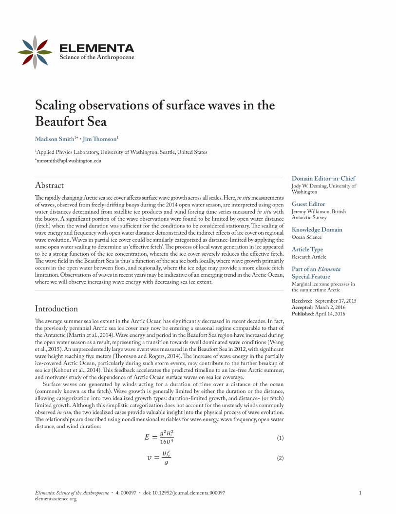
MethodsData collectionWave data were collected in the Beaufort Sea during the 2014 open water season using three Surface Wave Instrument Floats with Tracking (SWIFTs). SWIFTs are freely-drifting buoys that collect observations in ten-minute bursts at the top of each hour, and burst results are transmitted hourly via Iridium satellite antenna. SWIFTs 10 and 11 were deployed on July 27 from the R/V Ukpik roughly 100 km north of Alaska. They followed approximately the same path until September 1, when SWIFT 10 was caught in partial ice cover until September 15. Both buoys were recovered from the R/V Norseman II between September 28–29, 2014. SWIFT 15 was deployed and recovered from the R/V Araon from August 5 to 17, 2014, and was in partial ice cover the entirety of its deployment. Drift tracks of the SWIFTs are shown in Figure 1.

The wave-following reference frame of the SWIFT buoy allows wave spectra to be obtained from ocean surface velocities. The motion of the platform is measured using a GPS receiver (Microstrain 3DM-GX3-35) at 4 Hz, with a horizontal velocity precision of 0.05 m/s. Horizontal velocity vectors are decomposed into mean and wave orbital velocity components that are used to infer wave energy spectra (Herbers et al., 2012). The natural frequency of the buoy, with a period of 1.3 seconds, is damped by a small heave plate



to allow observations of wave motions from low frequency swells to high frequency wind waves. Wave energy spectra were calculated from ensemble averaging of fast Fourier transform (FFT) with an overlap of 50%. Significant wave height (Hs) and energy-weighted average period (Te) were obtained from the wave energy spectra. Significant wave height was determined in the frequency domain as four times the square root of the zeroth-moment of the wave spectra, m0 (i.e., the area under the wave spectra), or Hs = 4 √ 0. Energy-weighted average period was determined as the inverse of the energy-weighted frequency ( fe ), Te =

1fe

, with fe =

∑ Efm0

. Nondimensional wave energy and frequency were determined from Equations 1 and 2.

Wind speed, wind direction, and air temperature were collected at 1-meter mast height with an Airmar PB200 ultrasonic anemometer. Wind speeds were corrected to ten-meter wind speeds (U10) by assuming a logarithmic profile, where U10 = 1.35U1 (Benschop, 1996). Turbulent velocity profiles were measured using either a down-looking or High Resolution up-looking Nortek Aquadopp Doppler profiler in the lower hull. Additionally, photos were taken at 0.25 Hz during data collection bursts from a mast-mounted uCAM serial camera. A more detailed description of the SWIFT platform can be found in Thomson (2012). Time series of measured wind speed, significant wave height, energy-weighted period, and peak wave direction are shown in Figure 2. The anemometer and lower hull were lost from SWIFT 10 on September 15 as it exited the ice. As wind speed and wave directions are missing after this time, Navy Global Environmental Model (NAVGEM) wind speeds and wave direction were used instead (Hogan et al., 2014) and are differentiated in the figure by open circles.

Open water distance estimatesOpen water distances were estimated using a branched approach, differentiating between distances associated with waves measured in areas of open ocean and partial ice cover. Images from the camera onboard the SWIFT were used to determine whether measurements were taken in ice-free or partially ice-covered ocean (see Figures 3 and 4). Timelapse videos made from these images during the observations of SWIFT 10 and SWIFT 15 in partial ice are available as supplemental material (Videos S1 and S2).

When the onboard SWIFT images confirmed the absence of sea ice locally, open water distances were estimated using the daily 4 km National Ice Center’s (NIC) Multisensor Snow and Ice Mapping System (IMS) product, which uses a threshold of 15% ice concentration to determine the presence of ice (National Ice Center, 2008). The IMS product is produced from a human analysis of all available satellite image products, including visible, passive microwave, synthetic aperture radar (SAR), and radar scatterometer images, as well as snow mapping algorithms and other ancillary data, in order to give a relatively high resolution view of Arctic sea ice on a given day. The open water distance was calculated as the distance along the peak wave direction from the buoy to a land or ice boundary (Donelan et al., 1985). An example of the estimation of distance is shown in Figure 3 for SWIFT 11 on September 24, where the magenta line is the open water distance, x = 34 km. The nondimensional open water distance (χ) was then calculated using Equation 3. The relationship of nondimensional wave energy (E; Equation 1) and nondimensional open water distance in the Beaufort Sea was obtained using a least squares regression to the data.

Figure 1 Tracks of SWIFT drifters in the Beaufort Sea.

Thick colored lines mark the tracks of SWIFTs 11 (blue), 10 (red), and 15 (yellow). SWIFTs 11 and 10 were deployed from July 27 to September 29, and SWIFT 15 was deployed from August 5 to 17. Shown over fraction of sea ice cover on September 1, A, from AMSR2 sea ice product (Beitsch et al., 2013).doi: 10.12952/journal.elementa.000097.f001



When partial ice conditions were indicated by the SWIFT photos, nondimensional open water distance in the ice (χice) is determined using the fit from open water conditions. Nondimensional energy was calculated using the significant wave height, as in Equation 1. Then, the least squares regression relating nondimensional energy to nondimensional distance in open water was applied to find ‘effective’ nondimensional distance.

Estimates of χice were interpreted using the local percent ice concentration. The Advanced Microwave Scanning Radiometer 2 (AMSR2) passive microwave daily product from the University of Bremen (Beitsch et al., 2013), generated at a 6.25 km resolution using the ASI ice algorithm, was used to estimate ice cover as an average of all non-zero ice concentrations within a 30-km radius of the SWIFT location. Although the small field of view and low image resolution make it impossible to determine ice concentration from the onboard SWIFT images, they were used to qualitatively validate AMSR2 estimates. Figure 4 illustrates the estimation of ice concentration using AMSR2 for SWIFT 15, with validation from the SWIFT image.

Figure 3 Example calculation of open water distance.

Calculation of open water distance (fetch) for SWIFT 11 on September 24. Image taken from SWIFT confirms no local ice cover. Ice extent from NIC IMS product was used to calculate distance to the ice edge (magenta) in the peak wave direction. Here, fetch is x = 34 km.doi: 10.12952/journal.elementa.000097.f003

Figure 2 Wind and wave time series.

Time series of sea surface measurements during 2014 open water season from SWIFTs: (a) wind speed corrected to 10 m, (b) significant wave height, (c) energy-weighted wave period, and (d) peak wave direction (from 0 degrees North). Stars indicate winds from NAVGEM model outputs. Open circles indicate wave measurements made in partial ice cover.doi: 10.12952/journal.elementa.000097.f002

07/27 08/03 08/10 08/17 08/24 08/31 09/07 09/14 09/21 09/28 10/050

5

10

15

20W

ind

sp

ee

d,

U1

0 (

m/s

)

SWIFT 11SWIFT 10SWIFT 10 - NAVGEMSWIFT 15

07/27 08/03 08/10 08/17 08/24 08/31 09/07 09/14 09/21 09/28 10/050

1

2

3

4

5

Sig

wa

ve

he

igh

t, H

s (

m)

SWIFT 11SWIFT 10SWIFT 10 - iceSWIFT 15 - ice

07/27 08/03 08/10 08/17 08/24 08/31 09/07 09/14 09/21 09/28 10/05Time

4

6

8

10

En

erg

y-w

eig

hte

d p

erio

d,

Te (

s)

07/27 08/03 08/10 08/17 08/24 08/31 09/07 09/14 09/21 09/28 10/05Time

0

100

200

300

Wa

ve

dire

ctio

n (°)

(a)

(b)

(c)

(d)



We were also able to obtain concentrations from high-resolution Radarsat-2 (RS2) images for two cases in which images were collocated with SWIFT 10 in partial ice. RS2 images were thresholded with a level of 0.1 to separate ice floes from open water, and the portion of ice floes in a 30-km radius of the SWIFT was calculated. Error estimates in ice cover fraction were calculated as the standard deviation of ice concentration within the 30-km radius.

Results and analysesThe time series of winds and waves in Figure 2 show the range of conditions observed throughout the study period. Local ten-meter winds (Figure 2a) varied from just under 1 m/s to nearly 15 m/s. A few nonphysical wind measurements were removed in quality control. Two notable storms were captured, in early August and late September. Maximum wave heights (Figure 2b) occurred on September 28, at the end of the September storm, with a peak significant wave height of 4.6 m measured by SWIFT 11. Wave heights during the early August storm reached nearly 4 m. The wave characteristics from SWIFTs 10 and 11 roughly paralleled each other until September 1, when SWIFT 10 entered the MIZ (Figure 1). SWIFT 10 was in partial ice cover during the first two weeks of September, and SWIFT 15 was in ice the entirety of its mid-August deployment. These ice conditions were confirmed by the SWIFT onboard images (Videos S1 and S2). Wave characteristics measured in partial ice (indicated in the figure by open circles) have noticeably reduced significant wave heights and increased wave periods. Energy-weighted wave period in ice-free regions fluctuates between about 4 and 7 seconds, and reaches nearly 10 seconds in the ice (Figure 2c). Peak wave direction (Figure 2d) is primarily clustered around 100°, or approximately from the east.

Open water distancesDimensional open water distances derived using IMS ice extents are shown in Figure 5a. Here, we show all distances for both distance- and duration-limited wave conditions. The seasonal cycle of ice retreat and advance is evident, as open water distances increased towards mid-September and then began to decrease. This cycle corresponds with the measured minimum sea ice extent in this region, on September 16 (Fetterer et al., 2002). Additionally, the period of lowest ice extent corresponds to the greatest variability in open water distance.

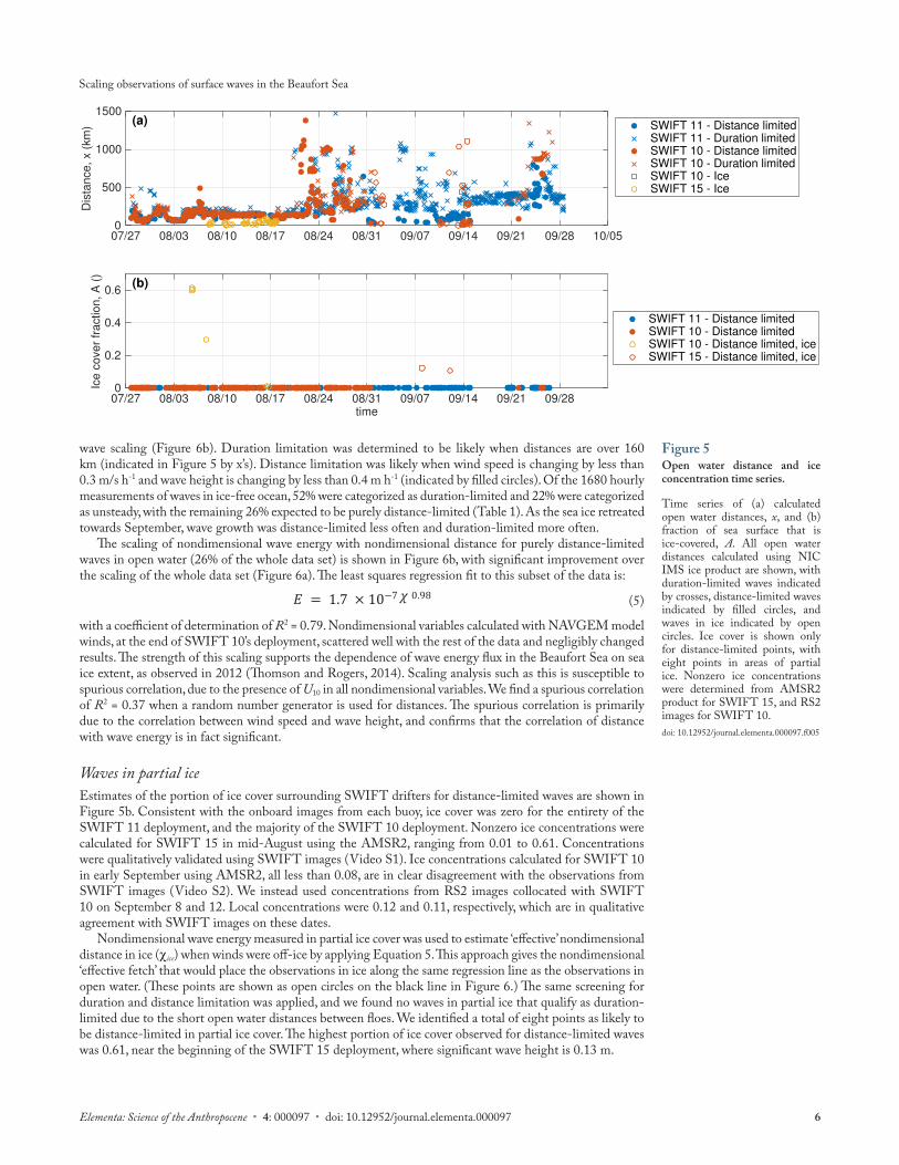
In Figure 6, we present scalings of wave energy with open water distance. The scaling in Figure 6a includes all distances determined, regardless of the limitation categorization as described below (i.e., 100% of the data set). The slope of the fit is χ0.88, with the coefficient of determination R2 = 0.64. A majority of the points with the largest errors are from the end of August, when there were large changes in wind speed and open water distance over short time scales. Nonstationarity in conditions resulted in poor correlation between open water distance and wave energy.

Exclusion of duration-limited conditionsBased on the descriptions of ideal duration- and distance-limited wave growth, we used an empirical approach to determine waves most likely to be duration-limited and distance-limited. We identified the waves that are most likely to be duration-limited as those with a large distance for wave generation and local wind speed greater than 5 m/s. From the remaining waves, distance limitation was most likely for waves with relatively stable wind speed and wave height. We empirically determined the cutoffs for minimum open water distance and maximum rate of change of wind speed and wave height by maximizing the fit of the distance-limited

Figure 4 Example calculation of local ice concentration.

Fraction of local sea ice cover, A, from AMSR2 for SWIFT 15 on August 6. Local ice concentration was determined by averaging nonzero ice concentrations within a 30-km radius of SWIFT. Here, local ice concentration was calculated as 0.60. Image taken from SWIFT qualitatively confirms this estimate.doi: 10.12952/journal.elementa.000097.f004



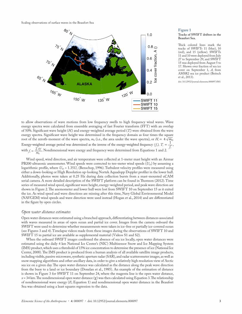
wave scaling (Figure 6b). Duration limitation was determined to be likely when distances are over 160 km (indicated in Figure 5 by x’s). Distance limitation was likely when wind speed is changing by less than 0.3 m/s h-1 and wave height is changing by less than 0.4 m h-1 (indicated by filled circles). Of the 1680 hourly measurements of waves in ice-free ocean, 52% were categorized as duration-limited and 22% were categorized as unsteady, with the remaining 26% expected to be purely distance-limited (Table 1). As the sea ice retreated towards September, wave growth was distance-limited less often and duration-limited more often.

The scaling of nondimensional wave energy with nondimensional distance for purely distance-limited waves in open water (26% of the whole data set) is shown in Figure 6b, with significant improvement over the scaling of the whole data set (Figure 6a). The least squares regression fit to this subset of the data is:

= 1.7 × 10 �−7 0.98 (5)

with a coefficient of determination of R2 = 0.79. Nondimensional variables calculated with NAVGEM model winds, at the end of SWIFT 10’s deployment, scattered well with the rest of the data and negligibly changed results. The strength of this scaling supports the dependence of wave energy flux in the Beaufort Sea on sea ice extent, as observed in 2012 (Thomson and Rogers, 2014). Scaling analysis such as this is susceptible to spurious correlation, due to the presence of U10 in all nondimensional variables. We find a spurious correlation of R2 = 0.37 when a random number generator is used for distances. The spurious correlation is primarily due to the correlation between wind speed and wave height, and confirms that the correlation of distance with wave energy is in fact significant.

Waves in partial iceEstimates of the portion of ice cover surrounding SWIFT drifters for distance-limited waves are shown in Figure 5b. Consistent with the onboard images from each buoy, ice cover was zero for the entirety of the SWIFT 11 deployment, and the majority of the SWIFT 10 deployment. Nonzero ice concentrations were calculated for SWIFT 15 in mid-August using the AMSR2, ranging from 0.01 to 0.61. Concentrations were qualitatively validated using SWIFT images (Video S1). Ice concentrations calculated for SWIFT 10 in early September using AMSR2, all less than 0.08, are in clear disagreement with the observations from SWIFT images (Video S2). We instead used concentrations from RS2 images collocated with SWIFT 10 on September 8 and 12. Local concentrations were 0.12 and 0.11, respectively, which are in qualitative agreement with SWIFT images on these dates.

Nondimensional wave energy measured in partial ice cover was used to estimate ‘effective’ nondimensional distance in ice (χice) when winds were off-ice by applying Equation 5. This approach gives the nondimensional ‘effective fetch’ that would place the observations in ice along the same regression line as the observations in open water. (These points are shown as open circles on the black line in Figure 6.) The same screening for duration and distance limitation was applied, and we found no waves in partial ice that qualify as duration-limited due to the short open water distances between floes. We identified a total of eight points as likely to be distance-limited in partial ice cover. The highest portion of ice cover observed for distance-limited waves was 0.61, near the beginning of the SWIFT 15 deployment, where significant wave height is 0.13 m.

Figure 5 Open water distance and ice concentration time series.

Time series of (a) calculated open water distances, x, and (b) fraction of sea surface that is ice-covered, A. All open water distances calculated using NIC IMS ice product are shown, with duration-limited waves indicated by crosses, distance-limited waves indicated by filled circles, and waves in ice indicated by open circles. Ice cover is shown only for distance-limited points, with eight points in areas of partial ice. Nonzero ice concentrations were determined from AMSR2 product for SWIFT 15, and RS2 images for SWIFT 10.doi: 10.12952/journal.elementa.000097.f005

07/27 08/03 08/10 08/17 08/24 08/31 09/07 09/14 09/21 09/28 10/050

500

1000

1500

Dis

tance, x (

km

) SWIFT 11 - Distance limitedSWIFT 11 - Duration limitedSWIFT 10 - Distance limitedSWIFT 10 - Duration limitedSWIFT 10 - IceSWIFT 15 - Ice

07/27 08/03 08/10 08/17 08/24 08/31 09/07 09/14 09/21 09/28time

0

0.2

0.4

0.6

Ice c

over

fraction, A

()

SWIFT 11 - Distance limitedSWIFT 10 - Distance limitedSWIFT 10 - Distance limited, iceSWIFT 15 - Distance limited, ice

(a)

(b)



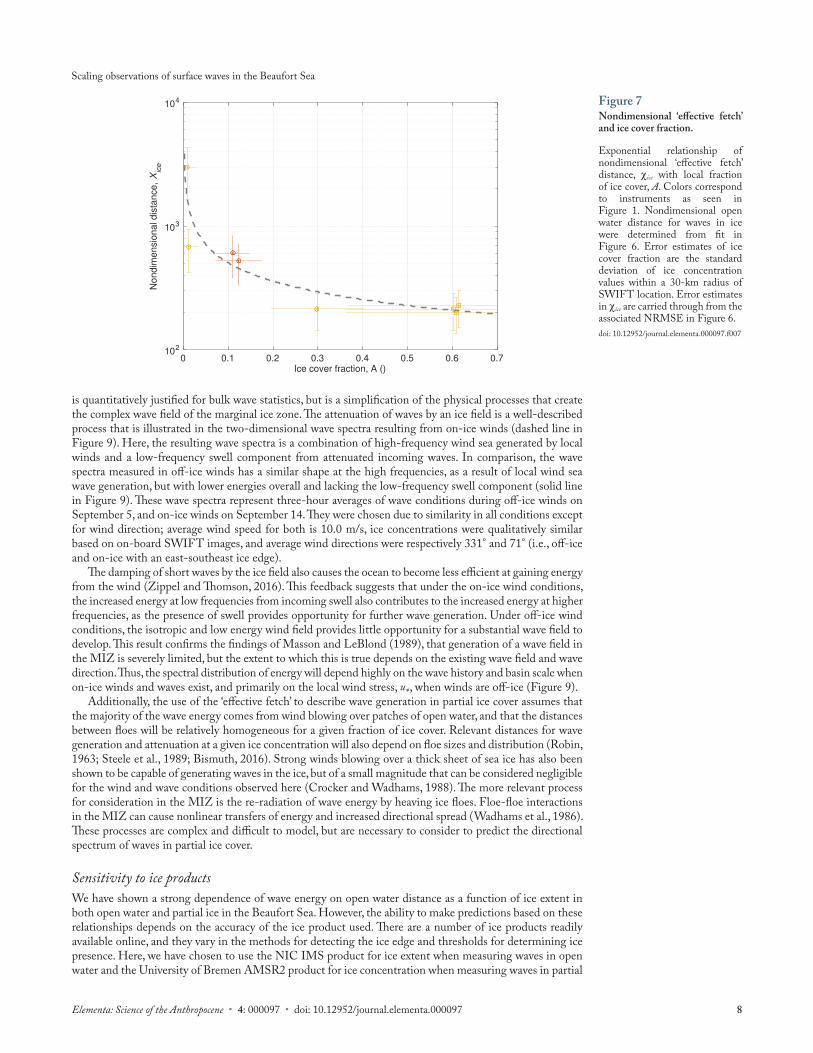
Comparison of the nondimensional ‘effective fetch’ in ice for distance-limited waves, χice, with local fraction of ice cover determined from AMSR2 and RS2 ice products, A, is shown in Figure 7. This comparison suggests that the ‘effective fetch’ rapidly decays with increasing ice fraction. Using a simple least squares regression to a power-law, the coefficient of determination is R2 = 0.82, and the relationship is:

= 162 −0.49� (6)

DiscussionWave evolutionThe observed relatively good correlation of the scaling of all open water wave measurements, regardless of qualification as distance- or duration-limited, indicates that the basin scale is often a limiting factor in open water wave development (i.e., that waves are rarely purely duration-limited; Figure 6a). The improvement of the regression by screening waves for duration limitation, wind stationarity, and ice absence does, however, shows a more nuanced dependence on open water distance (and one which is more consistent with true fetch limitation).

This result is similarly seen in the scaling of nondimensional open water distance (Equation 3) with nondimensional frequency (Equation 2), where there is an even stronger correlation of R2 = 0.87 (Figure 8). The trend is fit by the equation v = 4.0χ−0.33, which compares well with previous results from a fetch limitation experiment in Lake Ontario, where a fit of v = 1.85χ−0.23 was found (Donelan et al., 1985). The nondimensional frequency can be seen as an analog for the inverse wave age, where wave age is Teg

2πU10. Te is energy-weighted

average period and U10 is ten-meter wind speed, as earlier defined. The scaling then indicates that longer open water distances correspond with older waves. As the Arctic Ocean basin scale becomes larger with increased ice retreat, the wave field will be dominated by more mature swell waves. Older swell waves are likely to have come from further away in the basin, and thus are less correlated with local wind conditions.

While the energy balance governing ocean waves in open water depends on winds, nonlinear interactions, and breaking dissipation, the presence of sea ice introduces scattering and additional dissipation, and may also alter the wind, nonlinear interactions, and breaking dependencies themselves (Li et al., 2015; Zippel and Thomson, 2016). The use of the ‘effective fetch’ to describe waves generated in partially ice-covered ocean

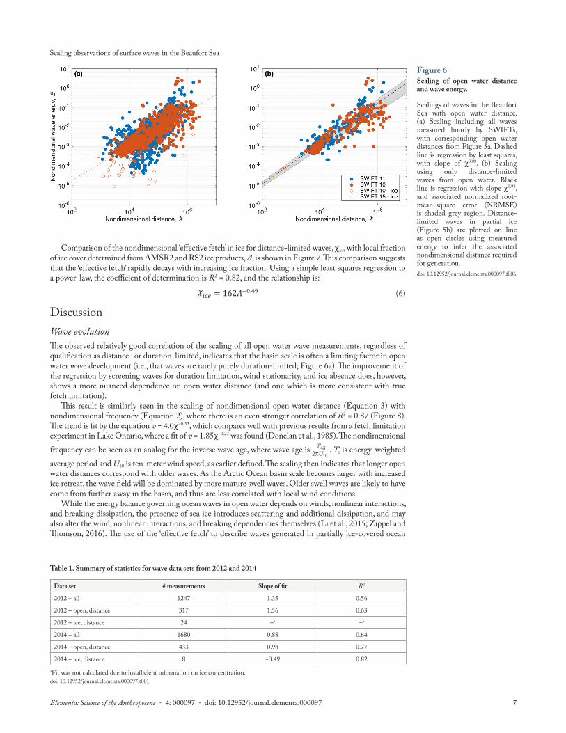
Table 1. Summary of statistics for wave data sets from 2012 and 2014

Data set # measurements Slope of fit R2

2012 – all 1247 1.35 0.56

2012 – open, distance 317 1.56 0.63

2012 – ice, distance 24 –a –a

2014 – all 1680 0.88 0.64

2014 – open, distance 433 0.98 0.77

2014 – ice, distance 8 −0.49 0.82aFit was not calculated due to insufficient information on ice concentration.doi: 10.12952/journal.elementa.000097.t001

Figure 6 Scaling of open water distance and wave energy.

Scalings of waves in the Beaufort Sea with open water distance. (a) Scaling including all waves measured hourly by SWIFTs, with corresponding open water distances from Figure 5a. Dashed line is regression by least squares, with slope of χ0.88. (b) Scaling using only distance-limited waves from open water. Black line is regression with slope χ0.98, and associated normalized root-mean-square error (NRMSE) is shaded grey region. Distance-limited waves in partial ice (Figure 5b) are plotted on line as open circles using measured energy to infer the associated nondimensional distance required for generation.doi: 10.12952/journal.elementa.000097.f006



is quantitatively justified for bulk wave statistics, but is a simplification of the physical processes that create the complex wave field of the marginal ice zone. The attenuation of waves by an ice field is a well-described process that is illustrated in the two-dimensional wave spectra resulting from on-ice winds (dashed line in Figure 9). Here, the resulting wave spectra is a combination of high-frequency wind sea generated by local winds and a low-frequency swell component from attenuated incoming waves. In comparison, the wave spectra measured in off-ice winds has a similar shape at the high frequencies, as a result of local wind sea wave generation, but with lower energies overall and lacking the low-frequency swell component (solid line in Figure 9). These wave spectra represent three-hour averages of wave conditions during off-ice winds on September 5, and on-ice winds on September 14. They were chosen due to similarity in all conditions except for wind direction; average wind speed for both is 10.0 m/s, ice concentrations were qualitatively similar based on on-board SWIFT images, and average wind directions were respectively 331° and 71° (i.e., off-ice and on-ice with an east-southeast ice edge).

The damping of short waves by the ice field also causes the ocean to become less efficient at gaining energy from the wind (Zippel and Thomson, 2016). This feedback suggests that under the on-ice wind conditions, the increased energy at low frequencies from incoming swell also contributes to the increased energy at higher frequencies, as the presence of swell provides opportunity for further wave generation. Under off-ice wind conditions, the isotropic and low energy wind field provides little opportunity for a substantial wave field to develop. This result confirms the findings of Masson and LeBlond (1989), that generation of a wave field in the MIZ is severely limited, but the extent to which this is true depends on the existing wave field and wave direction. Thus, the spectral distribution of energy will depend highly on the wave history and basin scale when on-ice winds and waves exist, and primarily on the local wind stress, u* , when winds are off-ice (Figure 9).

Additionally, the use of the ‘effective fetch’ to describe wave generation in partial ice cover assumes that the majority of the wave energy comes from wind blowing over patches of open water, and that the distances between floes will be relatively homogeneous for a given fraction of ice cover. Relevant distances for wave generation and attenuation at a given ice concentration will also depend on floe sizes and distribution (Robin, 1963; Steele et al., 1989; Bismuth, 2016). Strong winds blowing over a thick sheet of sea ice has also been shown to be capable of generating waves in the ice, but of a small magnitude that can be considered negligible for the wind and wave conditions observed here (Crocker and Wadhams, 1988). The more relevant process for consideration in the MIZ is the re-radiation of wave energy by heaving ice floes. Floe-floe interactions in the MIZ can cause nonlinear transfers of energy and increased directional spread (Wadhams et al., 1986). These processes are complex and difficult to model, but are necessary to consider to predict the directional spectrum of waves in partial ice cover.

Sensitivity to ice productsWe have shown a strong dependence of wave energy on open water distance as a function of ice extent in both open water and partial ice in the Beaufort Sea. However, the ability to make predictions based on these relationships depends on the accuracy of the ice product used. There are a number of ice products readily available online, and they vary in the methods for detecting the ice edge and thresholds for determining ice presence. Here, we have chosen to use the NIC IMS product for ice extent when measuring waves in open water and the University of Bremen AMSR2 product for ice concentration when measuring waves in partial

Figure 7 Nondimensional ‘effective fetch’ and ice cover fraction.

Exponential relationship of nondimensional ‘effective fetch’ distance, χice with local fraction of ice cover, A. Colors correspond to instruments as seen in Figure 1. Nondimensional open water distance for waves in ice were determined from fit in Figure 6. Error estimates of ice cover fraction are the standard deviation of ice concentration values within a 30-km radius of SWIFT location. Error estimates in χice are carried through from the associated NRMSE in Figure 6.doi: 10.12952/journal.elementa.000097.f007

0 0.1 0.2 0.3 0.4 0.5 0.6 0.7Ice cover fraction, A ()

102

103

104

Nondim

ensio

nal dis

tance,

Xic

e



ice cover, both of which utilize the ASI algorithm. These products were chosen based on product resolution, accessibility, and prevalence in relevant literature. Both methods have demonstrated skill at estimating ice coverage in the Arctic Ocean, and are capable of detecting thin and deteriorating ice as they are composites of multiple ice detection methods.

However, the disagreement of both IMS and AMSR2 ice products with observed ice conditions from the SWIFT mast camera and RS2 images on a number of occasions indicates that a bias exists on the local scale. The error estimates of ice concentration (Figure 7) range from 2% at low ice concentrations to 24% at high ice concentrations. In partially ice-covered oceans, small changes in the fraction of ice cover can significantly impact both generation and attenuation of wave energy. A recently published discussion of sea ice concentration products shows that the bias of ASI, utilized in the AMSR2 product used for SWIFT 15, is relatively high compared to other algorithms (Ivanova et al., 2015). The atmospheric interference at this frequency from clouds, particularly common in the MIZ, provides a significant source of error. Predictions of waves in ice-covered oceans might be improved by using ice concentration algorithms such as Bristol or CalVal with relatively low bias and standard deviation (Ivanova et al., 2015). Nonetheless, scalings presented here of open water waves based on distances from both IMS and AMSR2 ice products are successful, supporting previous indications that these readily available ice products are sufficient for large-scale prediction of waves in ice-free areas of the Arctic Ocean.

102 103 104 105 106 107

Nondimensional distance, X

10-2

10-1

100

Nondim

ensio

nal energ

y-w

eig

hte

d f

requency, ν

SWIFT 11SWIFT 10

Figure 8 Scaling of open water distance and frequency.

Scaling of waves in the Beaufort Sea, using nondimensional energy-weighted frequency versus nondimensional open water distance. Dashed line shows logarithmic regression to data with a slope of χ−0.33.doi: 10.12952/journal.elementa.000097.f008

Figure 9 Wave spectra in ice.

Wave spectral measurements from SWIFT 10 during off-ice wind conditions (solid line), where wave field is composed primarily of waves generated in partial ice cover by the ‘effective fetch’ between floes, and during on-ice wind conditions (dashed line), where wave signal is composed of both waves generated in partial ice and a low-frequency swell component from open water. Spectral measurements represent 3-hour averages.doi: 10.12952/journal.elementa.000097.f009

0.1 0.15 0.2 0.25 0.3 0.35 0.4 0.45Frequency (Hz)

10-5

10-4

10-3

10-2

10-1

100

101

En

erg

y (

m2/H

z)

Off ice windsOn ice winds



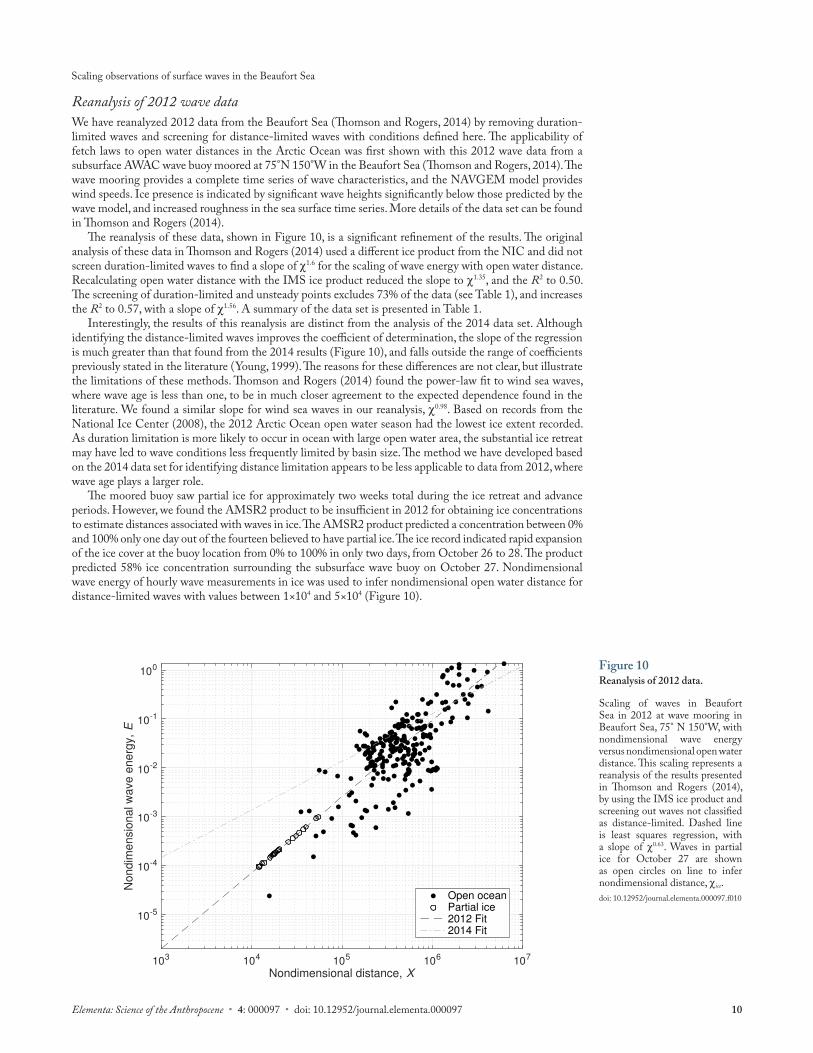
Reanalysis of 2012 wave dataWe have reanalyzed 2012 data from the Beaufort Sea (Thomson and Rogers, 2014) by removing duration-limited waves and screening for distance-limited waves with conditions defined here. The applicability of fetch laws to open water distances in the Arctic Ocean was first shown with this 2012 wave data from a subsurface AWAC wave buoy moored at 75°N 150°W in the Beaufort Sea (Thomson and Rogers, 2014). The wave mooring provides a complete time series of wave characteristics, and the NAVGEM model provides wind speeds. Ice presence is indicated by significant wave heights significantly below those predicted by the wave model, and increased roughness in the sea surface time series. More details of the data set can be found in Thomson and Rogers (2014).

The reanalysis of these data, shown in Figure 10, is a significant refinement of the results. The original analysis of these data in Thomson and Rogers (2014) used a different ice product from the NIC and did not screen duration-limited waves to find a slope of χ1.6 for the scaling of wave energy with open water distance. Recalculating open water distance with the IMS ice product reduced the slope to χ1.35, and the R2 to 0.50. The screening of duration-limited and unsteady points excludes 73% of the data (see Table 1), and increases the R2 to 0.57, with a slope of χ1.56. A summary of the data set is presented in Table 1.

Interestingly, the results of this reanalysis are distinct from the analysis of the 2014 data set. Although identifying the distance-limited waves improves the coefficient of determination, the slope of the regression is much greater than that found from the 2014 results (Figure 10), and falls outside the range of coefficients previously stated in the literature (Young, 1999). The reasons for these differences are not clear, but illustrate the limitations of these methods. Thomson and Rogers (2014) found the power-law fit to wind sea waves, where wave age is less than one, to be in much closer agreement to the expected dependence found in the literature. We found a similar slope for wind sea waves in our reanalysis, χ0.98. Based on records from the National Ice Center (2008), the 2012 Arctic Ocean open water season had the lowest ice extent recorded. As duration limitation is more likely to occur in ocean with large open water area, the substantial ice retreat may have led to wave conditions less frequently limited by basin size. The method we have developed based on the 2014 data set for identifying distance limitation appears to be less applicable to data from 2012, where wave age plays a larger role.

The moored buoy saw partial ice for approximately two weeks total during the ice retreat and advance periods. However, we found the AMSR2 product to be insufficient in 2012 for obtaining ice concentrations to estimate distances associated with waves in ice. The AMSR2 product predicted a concentration between 0% and 100% only one day out of the fourteen believed to have partial ice. The ice record indicated rapid expansion of the ice cover at the buoy location from 0% to 100% in only two days, from October 26 to 28. The product predicted 58% ice concentration surrounding the subsurface wave buoy on October 27. Nondimensional wave energy of hourly wave measurements in ice was used to infer nondimensional open water distance for distance-limited waves with values between 1×104 and 5×104 (Figure 10).

Figure 10 Reanalysis of 2012 data.

Scaling of waves in Beaufort Sea in 2012 at wave mooring in Beaufort Sea, 75° N 150°W, with nondimensional wave energy versus nondimensional open water distance. This scaling represents a reanalysis of the results presented in Thomson and Rogers (2014), by using the IMS ice product and screening out waves not classified as distance-limited. Dashed line is least squares regression, with a slope of χ0.63. Waves in partial ice for October 27 are shown as open circles on line to infer nondimensional distance, χice.doi: 10.12952/journal.elementa.000097.f010

103 104 105 106 107

Nondimensional distance, X

10-5

10-4

10-3

10-2

10-1

100

Nondim

ensio

nal w

ave e

nerg

y,

E

Open oceanPartial ice2012 Fit2014 Fit



Additionally, hourly wave measurements believed to be in 58% ice cover lie well above the line fit to nondimensional distance and ice concentration, in Figure 7. We hypothesize that this result is due to a difference in ice cover type, as these waves were measured during freezing conditions of ice advance. Wave spectra showed a high amount of damping at low frequencies (not shown), suggesting the possibility of shuga or frazil ice. This result illustrates the limitation of this method for sea ice types other than the brash ice identified in the 2014 measurements. A different relationship between ice cover and wave energy likely exists during ice freezing and advance.

ConclusionsWe have demonstrated a significant exponential relationship between the nondimensional wave energy and open water distances across the Beaufort Sea. Waves measured in both 2012 and 2014 in this region indicate that the hard ice edge limits fetch in a conventional manner. Scatter in the dataset indicates that the ocean rarely behaves in a purely distance-limited manner and will also be limited by wind duration. An empirical screening for relatively stationary winds and waves suggests that the likelihood of distance limitation decreases later in the summer and may decrease with reduced ice extent in general. Wave field observations during this year may be indicative of the new trend for waves in the emerging Arctic Ocean; with decreasing ice cover predicted, we are likely to observe more wave energy. The emergence of mature swell waves is notable, because these waves carry more energy flux (for a given height) and penetrate further into sea ice (e.g., Wadhams et al., 1988).

Wave energy in the Beaufort Sea is also controlled by sea ice extent in areas of partial ice cover. As originally suggested by Masson and LeBlond (1989) we observed that wind in the marginal ice zone is capable of generating very short, fetch-limited waves. In an MIZ with off-ice winds, wave generation is then a local process: waves are never duration-limited and are largely controlled by the distance between ice floes. Ice concentration, though not a perfect physical indicator of distance between floes, can be successfully used to indicate an ‘effective fetch’. When winds are on-ice, local generation of waves across the ‘effective fetch’ will be observed in addition to incident and attenuated waves from open water.

Application of this result is limited by the ice products presently available, which are sufficient for determining large scale ice extent, but not for local ice concentration and distance between floes. Currently, wave forecasts in ice by Wave-Watch 3 (WW3) simply scale inputs by the ice concentration. We have shown how the treatment of wind input can be improved in partial ice cover using the ice concentration, where wave energy is a function of open water distance between floes. However, it is clear that the physics of short, distance-limited waves in ice will not be described solely by the ice concentration. Physically accurate wave models will need to consider the interaction of waves and ice for wave scattering and regeneration. Additionally, the open water distance for wave generation in partial ice depends on the geometry of floes and floe size distribution. Efforts are currently being made to obtain better floe size distribution estimates from satellite images, which will serve to improve our understanding of wave generation in fractional ice cover (Zhang et al., 2015).

ReferencesBeitsch A, Kaleschke L, Kern S. 2013. AMSR2 ASI 3.125 km sea ice concentration data. University of Hamburg, Germany:

Institute of Oceanography. //ftp-projects.zmaw.de/seaice/.Benschop H. 1996. Windsnelheidsmetingen op zeestations en kuststations: Her-leiding waarden windsnelheid naar

10-meter niveau. Koninklijk Nederlands Meteorologisch Instituut Technical Report 188.Bismuth E. 2016. Interactions vagues-glace dans l’estuaire et le golfe du Saint-Laurent. Masters Thesis. Université du

Québec à Rimouski.Crocker GB, Wadhams P. 1988. Observations of wind-generated waves in Antarctic fast ice. J Phys Oceanogr 18: 1292.Donelan MA, Hamilton J, Hui WH. 1985. Directional spectra of wind-generated waves. P Roy Soc Lond A Mat 315(1534):

509–562.Fetterer F, Knowles K, Meier W, Savoie M. 2002. Sea Ice Index. Boulder, Colorado USA: National Snow and Ice Data

Center. http://dx.doi.org/10.7265/N5QJ7F7W. Updated daily.Herbers THC, Jessen PF, Janssen TT, Colbert DB, MacMahan JH. 2012. Observing ocean surface waves with GPS-tracked

buoys. J Atmos Ocean Tech 29: 944–959.Hogan T, Liu M, Ridout J, Peng M, Whitcomb T, et al. 2014. The Navy Global Environmental Model. Oceanography

27(3): 116–125.Ivanova N, Pedersen LT, Tonboe RT, Kern S, Heygster G, et al. 2015. Satellite passive microwave measurements of sea ice

concentration: An optimal algorithm and challenges. Cryosphere 9: 1797–1817.Kohout AL, Williams MJM, Dean SM, Meylan MH. 2014. Storm-induced sea-ice breakup and the implications for ice

extent. Nature 509: 604–607.Li J, Kohout AL, Shen HH. 2015. Comparison of wave propogation through ice covers in calm and storm conditions.

Geophys Res Lett 42.Martin T, Steele M, Zhang J. 2014. Seasonality and long-term trends of Arctic Ocean surface stress in a model. J Geophys

Res-Oceans 119.



Masson D, LeBlond PH. 1989. Spectral evolution of wind-generated surface gravity waves in a dispersed ice field. J Fluid Mech 202: 42–81.

Mitsuyasu H, Rikiishyi K. 1978. The growth of duration-limited wind waves. J Fluid Mech 85(4): 705–730.National Ice Center. 2008. IMS daily Northern Hemisphere snow and ice analysis at 1 km, 4 km, and 24 km resolutions.

Boulder, CO: National Snow and Ice Data Center. Digital Media. Updated daily.Robin GDQ. 1963. Wave propagation through fields of pack ice. P Roy Soc Lond A Mat 255(1057): 313–339.Squire V. 2007. Of ocean waves and sea-ice revisited. Cold Reg Sci Technol 49: 110–133.Squire V, Dugan J, Wadhams P, Rottier P, Liu A. 1995. Of ocean waves and sea-ice. Annu Rev Fluid Mech 27: 115–168.Steele M, Morison JH, Untersteiner N. 1989. The partition of air-ice-ocean momentum exchange as a function of ice

concentration, floe size, and draft. J Geophys Res 94(C9): 12739–12750.Thomson J. 2012. Wave breaking dissipation observed with “SWIFT” drifters. J Atmos Ocean Tech 29: 1866–1882.Thomson J, Rogers WE. 2014. Swell and sea in the emerging Arctic Ocean. Geophys Res Lett 14(9): 3136–3140.Wadhams P, Squire VA, Dougal DJ, Goodman J, Cowan AM, et al. 1988. The attenuation rates of ocean waves in the

marginal ice zone. J Geophys Res-Oceans 93(C6): 6799–6818.Wadhams P, Squire VA, Ewing JA, Pascal RW. 1986. The effect of the marginal ice zone on the directional wave spectrum

of the ocean. J Phys Oceanogr 16: 358–376.Wang XL, Feng Y, Swail VR, Cox A. 2015. Historical changes in the Beaufort-Chukchi-Bering Seas surface winds and

waves, 1971–2013. J Clim.Young I. 1999. Wind Generated Ocean Waves. Elsevier. (Ocean Engineering, vol. 2).Zhang J, Schweiger A, Steele M, Stern H. 2015. Sea ice floe size distribution in the marginal ice zone: Theory and numerical

experiments. J Geophys Res-Oceans 120(5): 3484–3498.Zippel S, Thomson J. 2016. Air-sea interactions in the marginal ice zone. Elem Sci Anth 4: 000095. doi: 10.12952/journal.

elementa.000095

Contributions• Contributed to conception and design: JT• Contributed to acquisition of data: JT, MS• Contributed to analysis and interpretation of data: MS, JT• Drafted and/or revised the article: MS, JT• Approved the submitted version for publication: JT, MS

AcknowledgmentsJoe Talbert and Alex DeKlerk designed, built, and deployed SWIFT drifters. The crews of the R/V Ukpik and R/V Norseman II assisted with deployment and recovery of SWIFTs 10 and 11. Craig Lee and the crew of the R/V Araon deployed SWIFT 15. Erick Rogers provided NAVGEM winds. Luc Rainville assisted with processing of ice products and satellite imagery. RadarSat2 images were provided by Hans Graber and Alexis Denton at the University of Miami.

Funding informationFunded by the Office of Naval Research (N00014-12-1-0113) as part of the Marginal Ice Zone program.

Competing interestsThe authors have no competing interests, as defined by Elementa, that might be perceived to influence the research presented in this manuscript.

Supplemental material• Video S1. Timelapse video of photos from SWIFT 15 mast-mounted serial camera showing deployment period in

partial ice Photos were taken at 0.25 Hz during hourly data collection from August 6 to August 18.

Video images were used for qualitative validation of satellite-derived ice concentrations. (MP4) doi: 10.12952/journal.elementa.000097.s001

• Video S2. Timelapse video of photos from SWIFT 10 mast-mounted serial camera showing period in partial ice cover

Photos were taken at 0.25 Hz during hourly data collection from September 1 to September 15, 2014. Video images were used for qualitative validation of satellite-derived ice concentrations. (MOV) doi: 10.12952/journal.elementa.000097.s002

Data accessibility statementSWIFT data available online: http://www.apl.uw.edu/swift

Copyright© 2016 Smith and Thomson. This is an open-access article distributed under the terms of the Creative Commons Attribution License, which permits unrestricted use, distribution, and reproduction in any medium, provided the original author and source are credited.

Scaling observations of surface waves in the Beaufort Sea

Documents