Bioreactor Scale-Up and CFD CFD- Computational Fluid Dynamics

Welcome message from author
This document is posted to help you gain knowledge. Please leave a comment to let me know what you think about it! Share it to your friends and learn new things together.
Transcript
Bioreactor Scale-Up and CFD
CFD- Computational Fluid Dynamics
What is Scale-up?
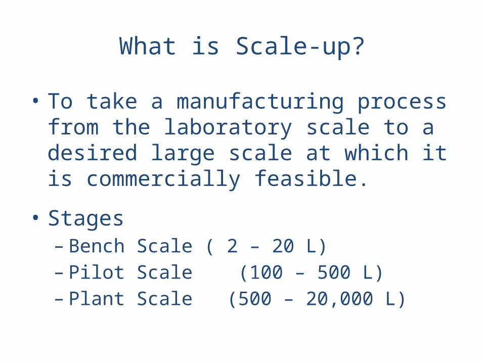
• To take a manufacturing process from the laboratory scale to a desired large scale at which it is commercially feasible.
• Stages– Bench Scale ( 2 – 20 L)– Pilot Scale (100 – 500 L)– Plant Scale (500 – 20,000 L)
What is Scale-up?
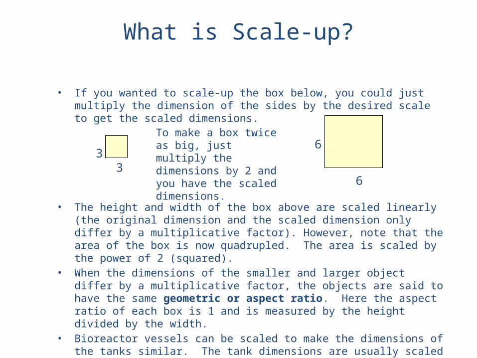
• If you wanted to scale-up the box below, you could just multiply the dimension of the sides by the desired scale to get the scaled dimensions.
• The height and width of the box above are scaled linearly (the original dimension and the scaled dimension only differ by a multiplicative factor). However, note that the area of the box is now quadrupled. The area is scaled by the power of 2 (squared).
• When the dimensions of the smaller and larger object differ by a multiplicative factor, the objects are said to have the same geometric or aspect ratio. Here the aspect ratio of each box is 1 and is measured by the height divided by the width.
• Bioreactor vessels can be scaled to make the dimensions of the tanks similar. The tank dimensions are usually scaled linearly, however the resulting tank volume does not scale linearly.
33 6
6
To make a box twice as big, just multiply the dimensions by 2 and you have the scaled dimensions.
What is Scale-up?
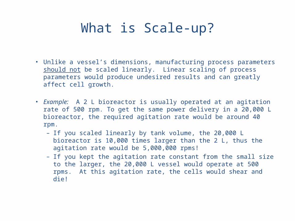
• Unlike a vessel’s dimensions, manufacturing process parameters should not be scaled linearly. Linear scaling of process parameters would produce undesired results and can greatly affect cell growth.
• Example: A 2 L bioreactor is usually operated at an agitation rate of 500 rpm. To get the same power delivery in a 20,000 L bioreactor, the required agitation rate would be around 40 rpm. – If you scaled linearly by tank volume, the 20,000 L bioreactor is 10,000 times larger than the 2 L, thus the agitation rate would be 5,000,000 rpms!
– If you kept the agitation rate constant from the small size to the larger, the 20,000 L vessel would operate at 500 rpms. At this agitation rate, the cells would shear and die!
Vessel Geometry
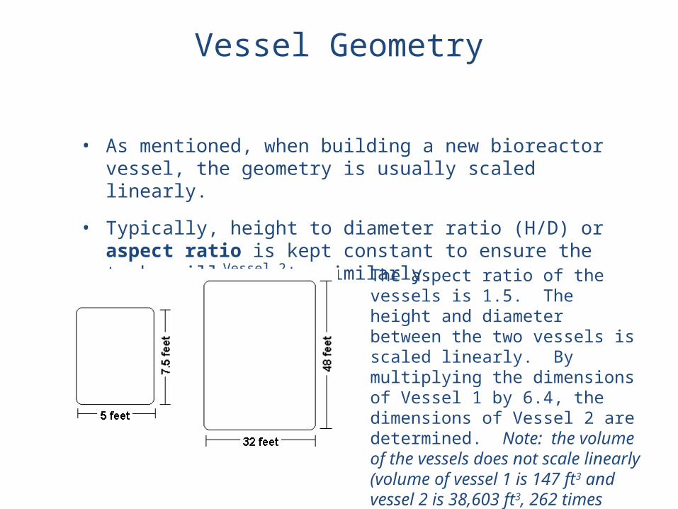
• As mentioned, when building a new bioreactor vessel, the geometry is usually scaled linearly.
• Typically, height to diameter ratio (H/D) or aspect ratio is kept constant to ensure the tanks will operate similarly.
Vessel 1
Vessel 2 The aspect ratio of the vessels is 1.5. The height and diameter between the two vessels is scaled linearly. By multiplying the dimensions of Vessel 1 by 6.4, the dimensions of Vessel 2 are determined. Note: the volume of the vessels does not scale linearly (volume of vessel 1 is 147 ft3 and vessel 2 is 38,603 ft3, 262 times larger.)
Process Parameters
• To scale-up a manufacturing process from one bioreactor to another, the process parameters are scaled based on the following :
• Agitation-based scaling parameters
• Gassing-based scaling parameters
Process Parameters
• Agitation-based scaling parameters:– Mixing Time– Power Input per Volume (P/V)– Tip Speed– Notes: These three parameters are all dependent on agitation
rate, so all three cannot be held constant when scaling-up. For example:
Keeping mixing time constant might cause a high P/V that the cells cannot handle.
Scaling based on constant tip speed might cause a low agitation rate that will not deliver oxygen adequately.
- Thus all three scaling parameters must be evaluated and the final scale-up agitation rate must produce acceptable values for all three parameters.
Process Parameters
• Gassing-based scaling parameters– Vessel Volumes per Minute, VVM– Superficial Gas Velocity, Vs– Note: The two gas flow rate scaling parameters are both
dependent on the dimensions of the vessel. Scaling based on one will greatly affect the other.
Agitation Speed: Scale-up Based on Mixing Time
• Mixing time is the amount of time it takes the bioreactor to create a homogeneous environment.
• Mixing time is usually measured by adding a concentrated salt solution to the bioreactor full of water and recording the conductivity (salt concentration) until it reaches a steady value. The elapsed time from introduction of the salt solution to achieving a constant conductivity reading in the bioreactor is the mixing time.
• Mixing time is important. When adding components such as feed or base to the bioreactor, you want to ensure that they mix in a timely manner. This way local regions of high or low pH and/or nutrients are not formed.
• Proper mixing time also ensures adequate oxygen delivery to the cells.
Agitation Speed: Scale-up Based on Mixing Time
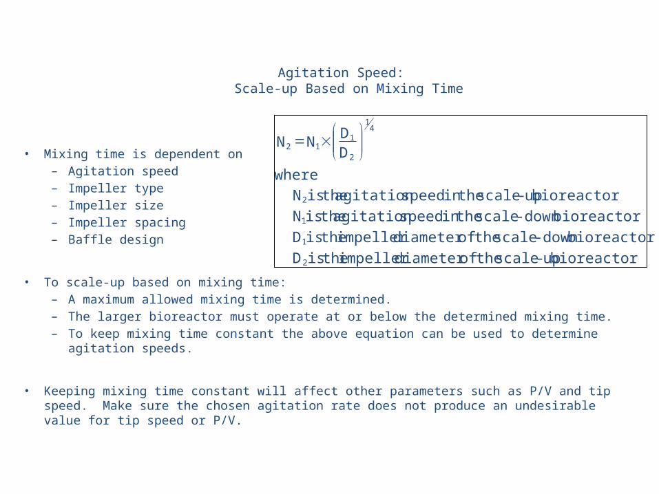
• Mixing time is dependent on– Agitation speed– Impeller type– Impeller size– Impeller spacing– Baffle design
• To scale-up based on mixing time:– A maximum allowed mixing time is determined.– The larger bioreactor must operate at or below the determined mixing time.– To keep mixing time constant the above equation can be used to determine
agitation speeds.
• Keeping mixing time constant will affect other parameters such as P/V and tip speed. Make sure the chosen agitation rate does not produce an undesirable value for tip speed or P/V.
bioreactor up-scale the of diameter impeller the is D bioreactor down-scale the of diameter impeller the is D
bioreactor down-scale the in speed agitation the is N bioreactor up-scale the in speed agitation the is N
whereDDNN
2
1
1
2
41
2
112 ÷÷ø
öççè
æ´=
Agitation Speed: Scale-up Based on P/V
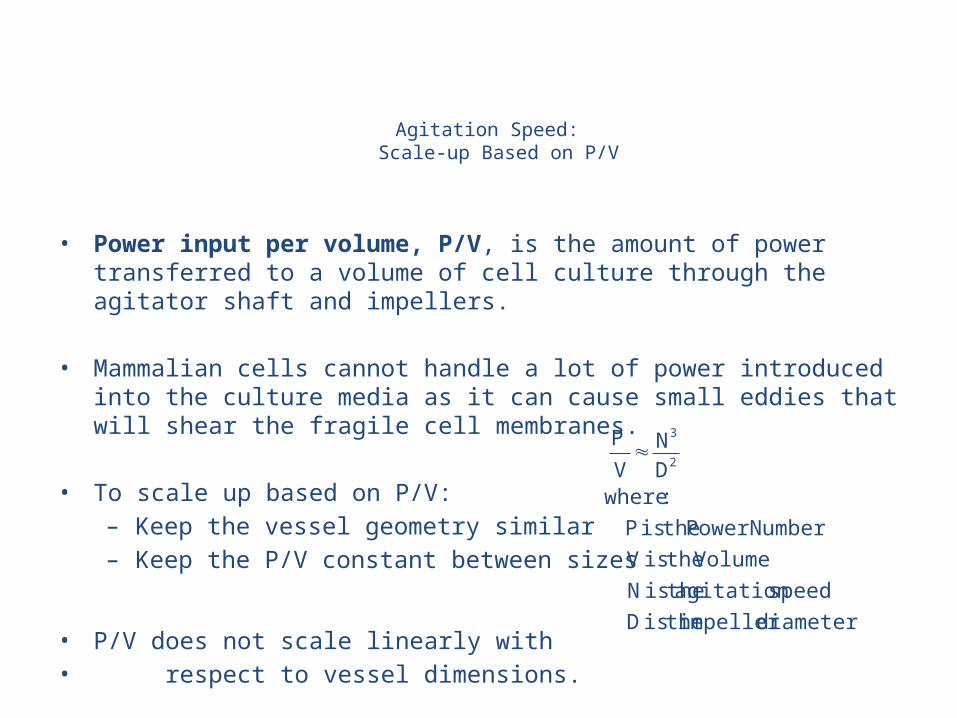
• Power input per volume, P/V, is the amount of power transferred to a volume of cell culture through the agitator shaft and impellers.
• Mammalian cells cannot handle a lot of power introduced into the culture media as it can cause small eddies that will shear the fragile cell membranes.
• To scale up based on P/V:– Keep the vessel geometry similar – Keep the P/V constant between sizes
• P/V does not scale linearly with • respect to vessel dimensions.
diameterimpeller theis D speedagitation theis N
Volume theis V NumberPower theis P
:whereDN
VP
2
3»
Agitation Speed: Scale-up Based on P/V
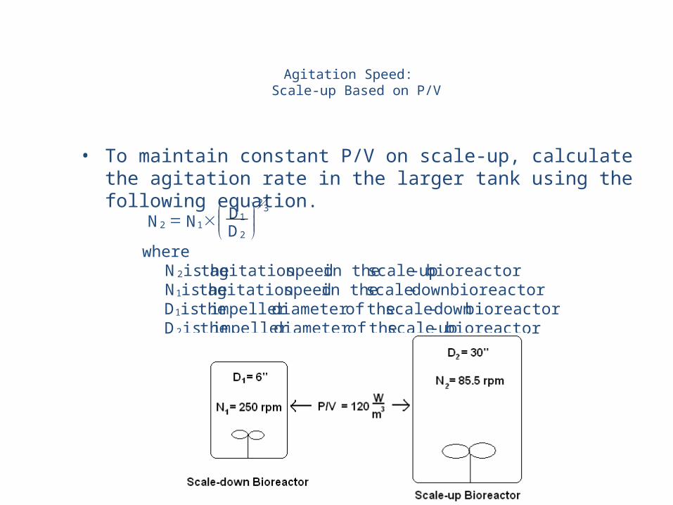
• To maintain constant P/V on scale-up, calculate the agitation rate in the larger tank using the following equation.
bioreactor up-scale theofdiameter impeller theis D bioreactordown -scale theofdiameter impeller theis D
bioreactordown -scale in the speedagitation theis N bioreactor up-scale in the speedagitation theis N
whereDDNN
2
1
1
2
32
21
12 ÷÷øö
ççèæ´=
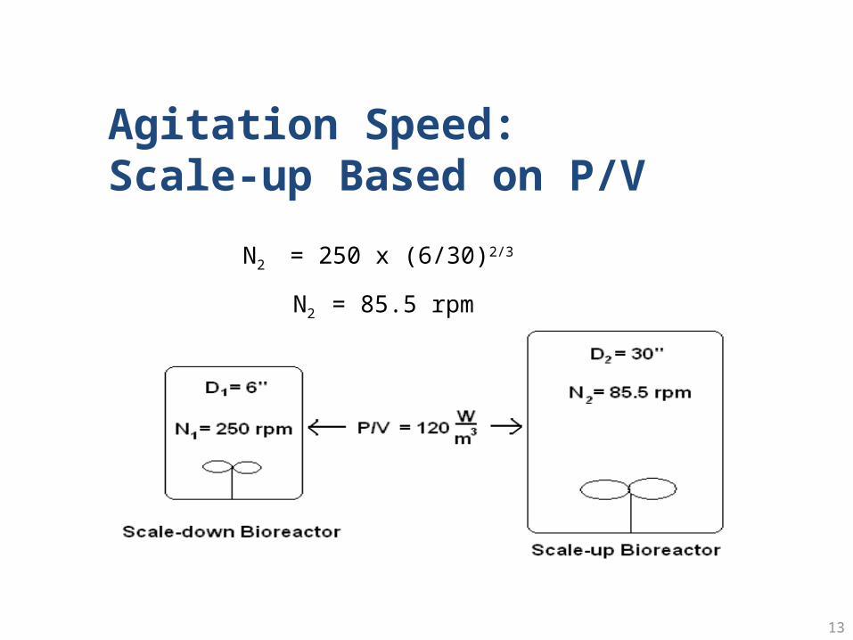
13
N2 = 250 x (6/30)2/3
N2 = 85.5 rpm
Agitation Speed: Scale-up Based on P/V
Agitation Speed: Scale-up Based on Tip Speed
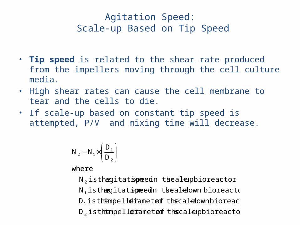
• Tip speed is related to the shear rate produced from the impellers moving through the cell culture media.
• High shear rates can cause the cell membrane to tear and the cells to die.
• If scale-up based on constant tip speed is attempted, P/V and mixing time will decrease.
bioreactor up-scale theofdiameter impeller theis D bioreactordown -scale theofdiameter impeller theis D
bioreactordown -scale in the speedagitation theis N bioreactor up-scale in the speedagitation theis N
whereDDNN
2
1
1
2
2
112 ÷÷
ø
öççè
æ´=
Gas Flow Rate: Scale-up Based on VVM
• Vessel Volumes per Minute, VVM, means the volume of gas flow (usually measured in slpm, standard liters per minute) per bioreactor volume per minute.
• Scaling-up the gas flow rate is necessary to ensure that enough oxygen will be supplied to the cells
• VVM is dependent on the volume of the vessel.• Typically cell culture processes maintain
around 0.1 – 0.2 VVM. This means that a 100 L vessel would have a maximum gas flow rate around 20 slpm.
Gas Flow Rate: Scale-up Based on Superficial Gas Velocity
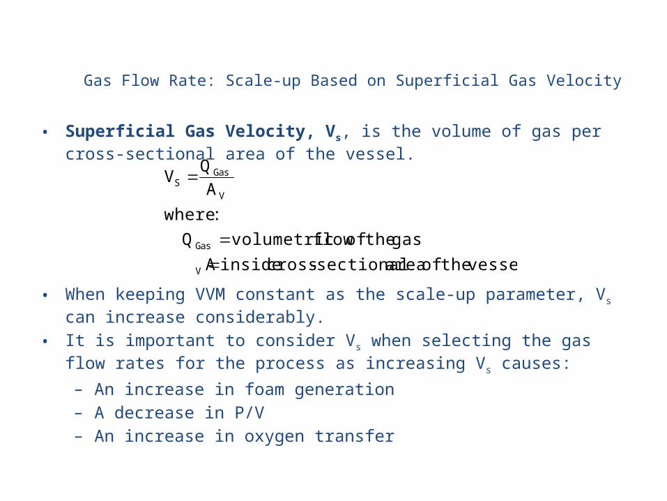
• Superficial Gas Velocity, Vs, is the volume of gas per cross-sectional area of the vessel.
• When keeping VVM constant as the scale-up parameter, Vs can increase considerably.
• It is important to consider Vs when selecting the gas flow rates for the process as increasing Vs causes:– An increase in foam generation– A decrease in P/V– An increase in oxygen transfer
vessel the of area sectional-cross inside Agas the offlow volumetric Q
:whereAQ V
V
Gas
V
GasS
==
=
Scale-Up Review
• Overall, scaling up process parameters is tricky.
• Each scale-up parameter is dependent on another. Scaling-up based on constant P/V will affect the mixing time and the tip speed in the bioreactor. As well, for gas flow rates, scaling-up on constant Vs will affect the VVM.
• Not one scale-up process is correct; the technical transfer team must study the effect of each scale-up parameter on the process to ensure there are no adverse effects.
Computational Fluid Dynamics
19
Computational Fluid Dynamics
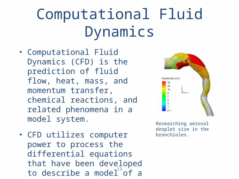
• Computational Fluid Dynamics (CFD) is the prediction of fluid flow, heat, mass, and momentum transfer, chemical reactions, and related phenomena in a model system.
• CFD utilizes computer power to process the differential equations that have been developed to describe a model of a system
Researching aerosol droplet size in the bronchioles.
20
History and Application of CFD
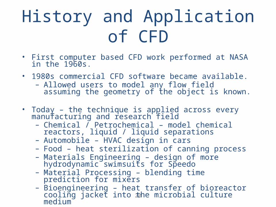
• First computer based CFD work performed at NASA in the 1960s.
• 1980s commercial CFD software became available.– Allowed users to model any flow field assuming the geometry of the object is known.
• Today – the technique is applied across every manufacturing and research field– Chemical / Petrochemical – model chemical reactors, liquid / liquid separations
– Automobile – HVAC design in cars– Food – heat sterilization of canning process– Materials Engineering – design of more hydrodynamic swimsuits for Speedo
– Material Processing – blending time prediction for mixers
– Bioengineering – heat transfer of bioreactor cooling jacket into the microbial culture medium
21
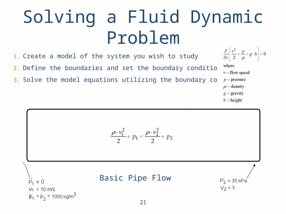
Solving a Fluid Dynamic Problem
Basic Pipe Flow
1. Create a model of the system you wish to study2. Define the boundaries and set the boundary conditions.3. Solve the model equations utilizing the boundary conditions.
Velocity at the exit of the pipe = 5.5 m/s2
22
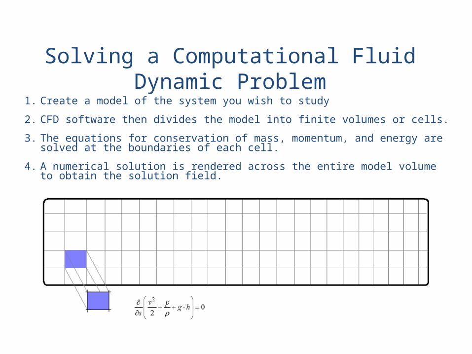
Solving a Computational Fluid Dynamic Problem
1. Create a model of the system you wish to study2. CFD software then divides the model into finite volumes or cells.3. The equations for conservation of mass, momentum, and energy are
solved at the boundaries of each cell. 4. A numerical solution is rendered across the entire model volume
to obtain the solution field.
Basic Pipe Flow
23
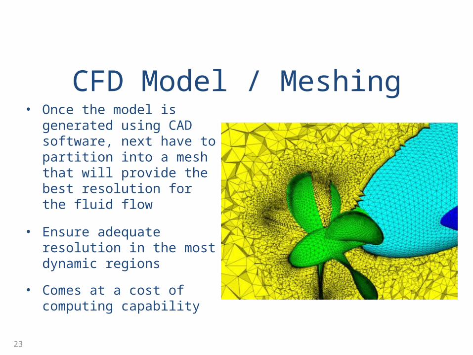
CFD Model / Meshing• Once the model is
generated using CAD software, next have to partition into a mesh that will provide the best resolution for the fluid flow
• Ensure adequate resolution in the most dynamic regions
• Comes at a cost of computing capability
24
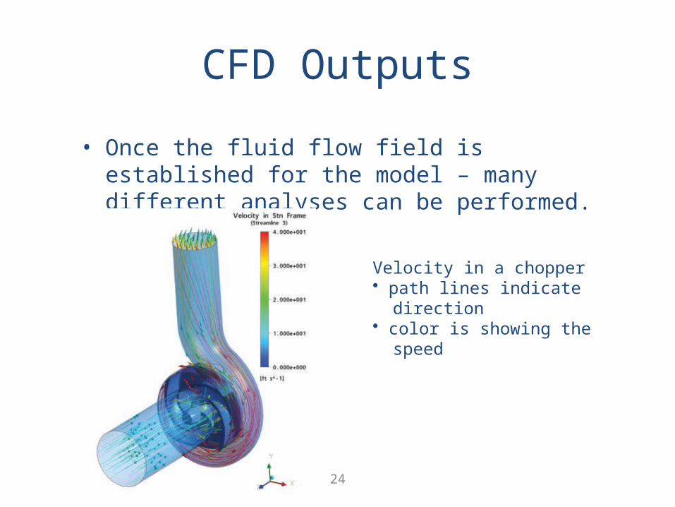
• Once the fluid flow field is established for the model – many different analyses can be performed.
Velocity in a chopper• path lines indicate direction• color is showing the speed
CFD Outputs
25
CFD Outputs
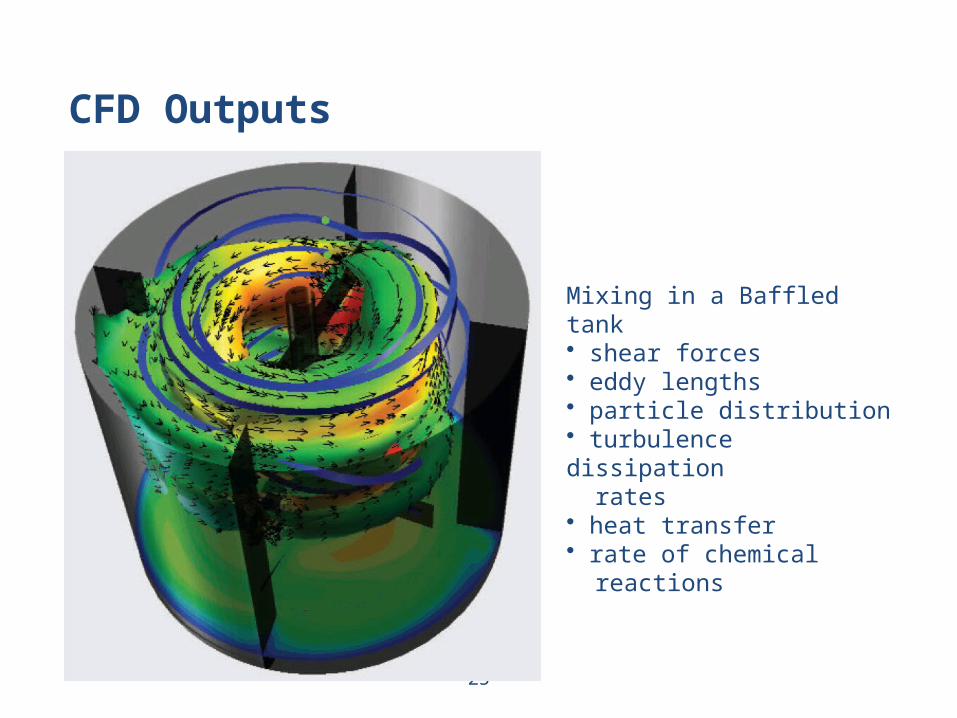
Mixing in a Baffled tank• shear forces• eddy lengths• particle distribution• turbulence dissipation rates• heat transfer• rate of chemical reactions
26
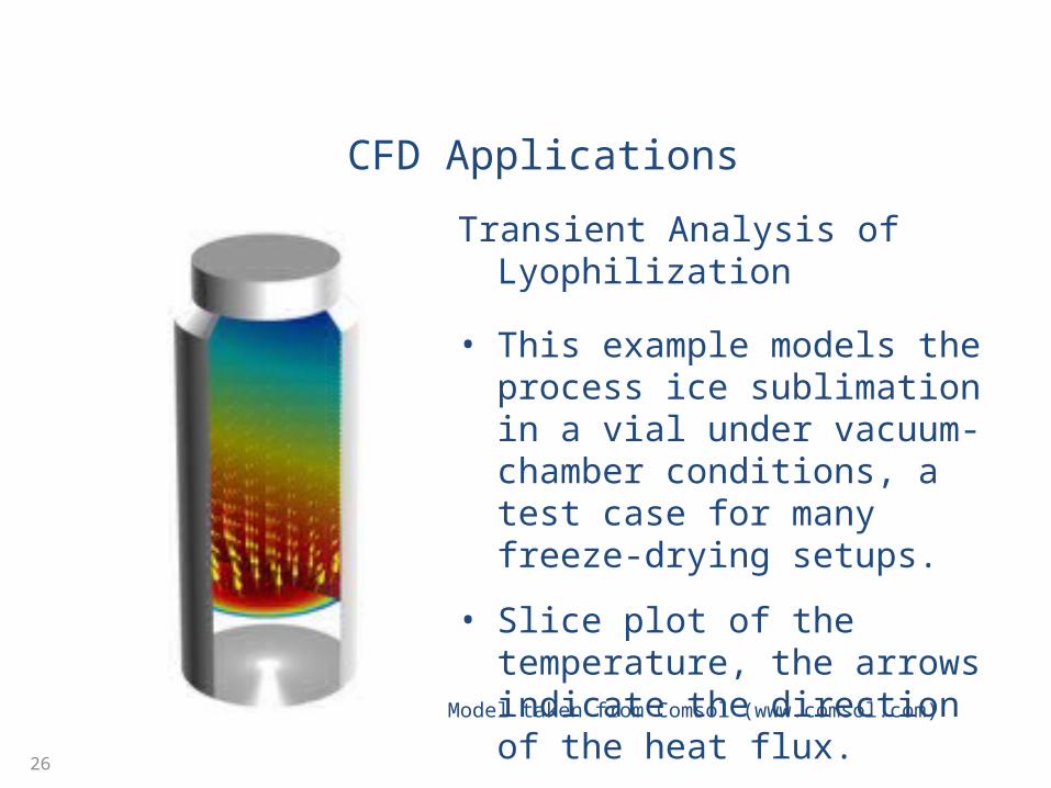
CFD ApplicationsTransient Analysis of Lyophilization
• This example models the process ice sublimation in a vial under vacuum-chamber conditions, a test case for many freeze-drying setups.
• Slice plot of the temperature, the arrows indicate the direction of the heat flux.
Model taken from Comsol (www.comsol.com)
27
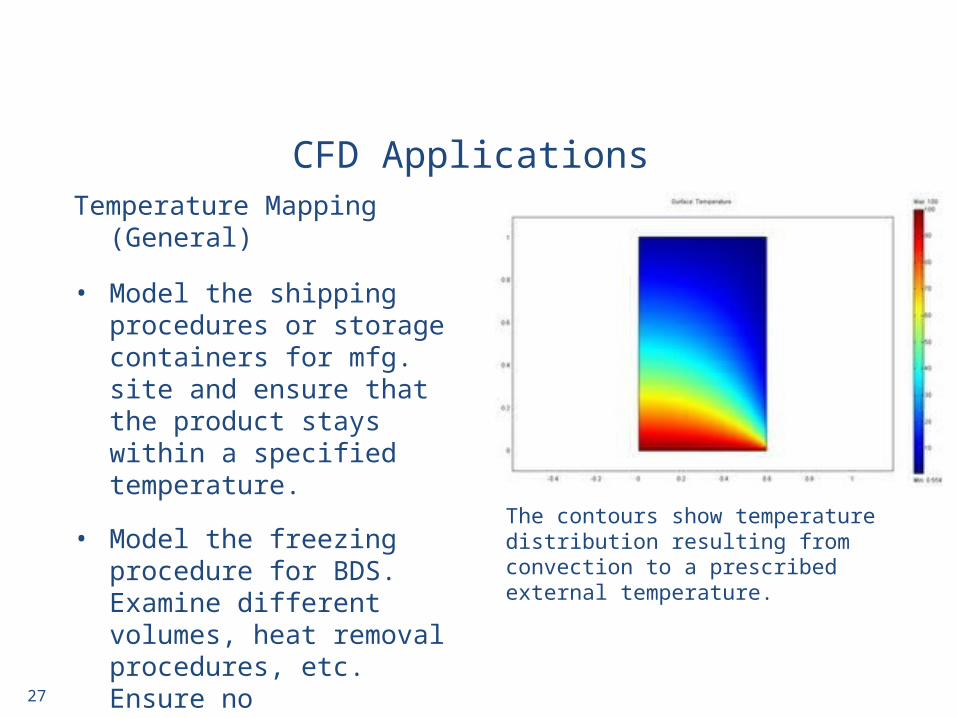
CFD ApplicationsTemperature Mapping
(General)
• Model the shipping procedures or storage containers for mfg. site and ensure that the product stays within a specified temperature.
• Model the freezing procedure for BDS. Examine different volumes, heat removal procedures, etc. Ensure no crystallization of the product occurs.
The contours show temperature distribution resulting from convection to a prescribed external temperature.
28
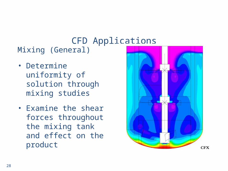
CFD ApplicationsMixing (General)
• Determine uniformity of solution through mixing studies
• Examine the shear forces throughout the mixing tank and effect on the product
CFD Helping Scale-up Issues
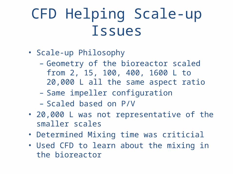
• Scale-up Philosophy– Geometry of the bioreactor scaled from 2, 15, 100, 400, 1600 L to 20,000 L all the same aspect ratio
– Same impeller configuration– Scaled based on P/V
• 20,000 L was not representative of the smaller scales
• Determined Mixing time was criticial• Used CFD to learn about the mixing in the bioreactor
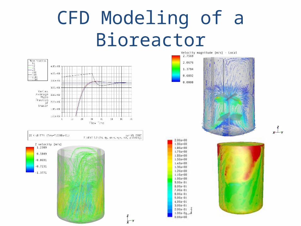
CFD Modeling of a Bioreactor
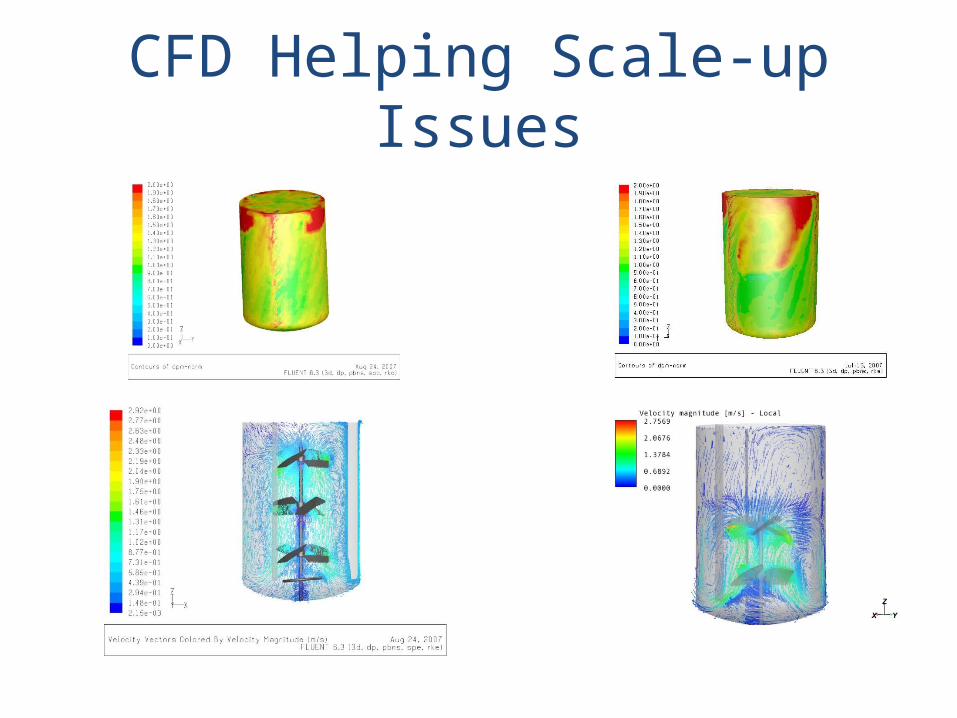
CFD Helping Scale-up Issues
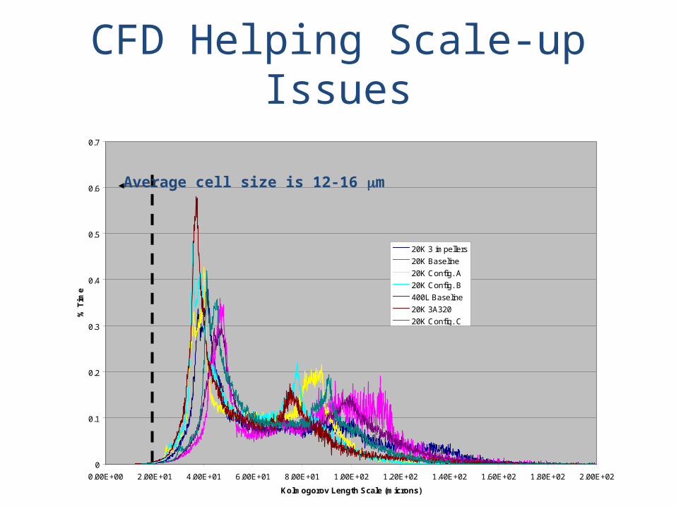
CFD Helping Scale-up Issues
0
0.1
0.2
0.3
0.4
0.5
0.6
0.7
0.00E+00 2.00E+01 4.00E+01 6.00E+01 8.00E+01 1.00E+02 1.20E+02 1.40E+02 1.60E+02 1.80E+02 2.00E+02Kolm ogorov Length Scale (m icrons)
% Time
20K 3 im pellers20K Baseline20K Config. A 20K Config. B400L Baseline20K 3A32020K Config. C
Average cell size is 12-16 mm
33
Overall Benefit of CFD• Able to develop a virtual model of your system of study
• Perform virtual experiments in the model that are difficult to perform in the actual system
• Allows one to evaluate many changes, configurations, and set-up in minimal time
• Gain a picture of the 3D space that is difficult to quantify experimentally
34
Drawbacks of CFD• Need CAD experience – develop the model
• Need the meshing knowledge• Need fluid dynamics experience – develop the equations for what you are wanting to model
• Need a lot of computing capacity
• Many consultants working in this field to help companies reach their goals!
Related Documents


