arXiv:1104.4991v1 [cond-mat.stat-mech] 26 Apr 2011 S CALE I NVARIANT A VALANCHES : AC RITICAL C ONFUSION Osvanny Ramos ∗ Laboratoire PMMH, ESPCI, CNRS UMR 7636, 10 rue Vauquelin, 75231 Paris Cedex 05, France. Laboratoire PMCN, Universit´ e Lyon 1, CNRS UMR 5586, 43 Bld. du 11 novembre 1918, 69622 Villeurbanne, France November 7, 2018 Abstract The “Self-organized criticality” (SOC), introduced in 1987 by Bak, Tang and Wiesenfeld, was an attempt to explain the 1/f noise, but it rapidly evolved towards a more ambitious scope: explaining scale invariant avalanches. In two decades, phe- nomena as diverse as earthquakes, granular piles, snow avalanches, solar flares, su- perconducting vortices, sub-critical fracture, evolution, and even stock market crashes have been reported to evolve through scale invariant avalanches. The theory, based on the key axiom that a critical state is an attractor of the dynamics, presented an expo- nent close to −1 (in two dimensions) for the power-law distribution of avalanche sizes. However, the majority of real phenomena classified as SOC present smaller exponents, i.e., larger absolute values of negative exponents, a situation that has provoked a lot of confusion in the field of scale invariant avalanches. The main goal of this chapter is to shed light on this issue. The essential role of the exponent value of the power-law distribution of avalanche sizes is discussed. The exponent value controls the ratio of small and large events, the energy balance –required for stationary systems– and the critical properties of the dynamics. A condition of criticality is introduced. As the ex- ponent value decreases, there is a decrease of the critical properties, and consequently the system becomes, in principle, predictable. Prediction of scale invariant avalanches in both experiments and simulations are presented. Other sources of confusion as the use of logarithmic scales, and the avalanche dynamics in well established critical systems, are also revised; as well as the influence of dissipation and disorder in the “self-organization” of scale invariant dynamics. PACS 05.65.+b, 91.30.Ab, 45.70.-n, 45.70.Ht * E-mail: [email protected]

Welcome message from author
This document is posted to help you gain knowledge. Please leave a comment to let me know what you think about it! Share it to your friends and learn new things together.
Transcript
arX
iv:1
104.
4991
v1 [
cond
-mat
.sta
t-m
ech]
26
Apr
201
1
SCALE I NVARIANT AVALANCHES :A CRITICAL CONFUSION
Osvanny Ramos∗
Laboratoire PMMH, ESPCI, CNRS UMR 7636,10 rue Vauquelin, 75231 Paris Cedex 05, France.
Laboratoire PMCN, Universite Lyon 1, CNRS UMR 5586,43 Bld. du 11 novembre 1918, 69622 Villeurbanne, France
November 7, 2018
Abstract
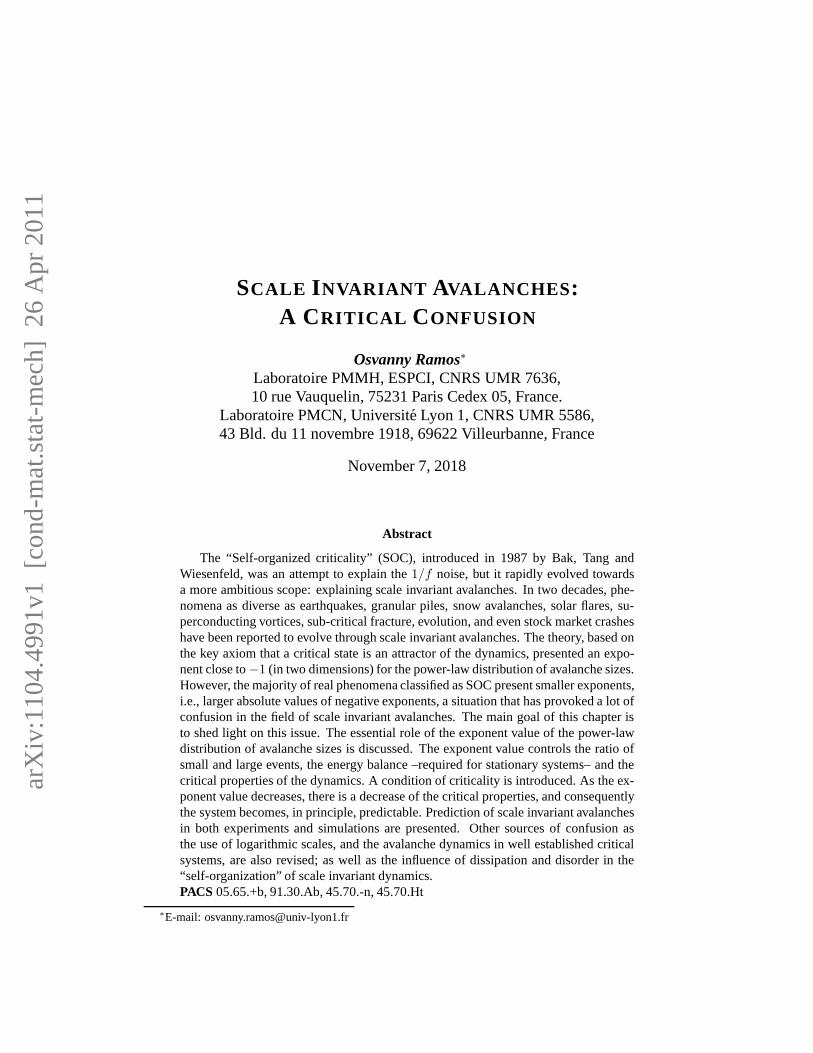
The “Self-organized criticality” (SOC), introduced in 1987 by Bak, Tang andWiesenfeld, was an attempt to explain the1/f noise, but it rapidly evolved towardsa more ambitious scope: explaining scale invariant avalanches. In two decades, phe-nomena as diverse as earthquakes, granular piles, snow avalanches, solar flares, su-perconducting vortices, sub-critical fracture, evolution, and even stock market crasheshave been reported to evolve through scale invariant avalanches. The theory, based onthe key axiom that a critical state is an attractor of the dynamics, presented an expo-nent close to−1 (in two dimensions) for the power-law distribution of avalanche sizes.However, the majority of real phenomena classified as SOC present smaller exponents,i.e., larger absolute values of negative exponents, a situation that has provoked a lot ofconfusion in the field of scale invariant avalanches. The main goal of this chapter isto shed light on this issue. The essential role of the exponent value of the power-lawdistribution of avalanche sizes is discussed. The exponentvalue controls the ratio ofsmall and large events, the energy balance –required for stationary systems– and thecritical properties of the dynamics. A condition of criticality is introduced. As the ex-ponent value decreases, there is a decrease of the critical properties, and consequentlythe system becomes, in principle, predictable. Predictionof scale invariant avalanchesin both experiments and simulations are presented. Other sources of confusion asthe use of logarithmic scales, and the avalanche dynamics inwell established criticalsystems, are also revised; as well as the influence of dissipation and disorder in the“self-organization” of scale invariant dynamics.PACS05.65.+b, 91.30.Ab, 45.70.-n, 45.70.Ht
∗E-mail: [email protected]

2 O. Ramos
Keywords: avalanches, scale invariance, Self-organized Criticality, avalanche predic-tion.
1. Introduction
“But he hasn’t got anything on,” a little child said.Hans Christian Andersen inThe Emperor’s New Clothes
Scale invariance pervades nature, both in space and time. Inspace, it is revealedthrough the ubiquity of fractal structures; and in time, with the presence of scale invari-ant avalanches. Avalanches can be seen as sudden liberations of energy which has beenaccumulated very slowly1; and phenomena as diverse as earthquakes [1, 2, 3], granularpiles [4, 5, 6, 7, 8, 9, 11, 11, 12], snow avalanches [13], solar flares [14], superconductingvortices [15, 16, 17, 18], sub-critical fracture [19], evolution [20], and even stock marketcrashes [21] have been reported to evolve through scale invariant avalanches. The signatureof the scale invariance corresponds to a power-law in the distribution of avalanche sizes,however, the exponents of the power-laws present in generaldifferent values. In 1987, PerBak and co-workers introduced the “Self-organized criticality” (SOC) as an explanationof scale invariance in nature [22]. The SOC proposes a mapping between scale invariantavalanches and critical phenomena, with the key axiom that the critical state is an attrac-tor of the dynamics, provoking the self-organization of thesystem towards a critical state[23, 24].
However, the axiomatic manner in which the base of the theorywas introduced, setSOC as a theory to be proved more than as a theory to develop. Many theoretical studiesfocused on mapping SOC into the formalism of critical points[25, 26, 27]; others, ondeveloping models displaying SOC behavior [1, 15, 20], increasing the members of the SOCfamily. However, the number of experiments were rather small, and they focused mainly onvalidating the theory, where the main goal was to find power-law distributions of avalanches[4, 5, 6, 7]. The original work presented an exponent close to−1 (in two dimensions),while many of the experimental and numerical results displayed smaller values, i.e., largerabsolute values of negative exponents. Regardless this difference, they were classified asSOC, having as a “heritage” all the critical properties of the original model, thus bringing alot of confusion to the field of scale invariant avalanches. The main goal of this chapter isto shed light on this issue.
The essential role of the exponent of the power-law in the dynamics is the first subjectof discussion. The exponent value controls the ratio of small and large events, the energybalance –required for stationary systems– and the criticalproperties of the dynamics. Thecauses and consequences of a logarithmic scale, which is a source of confusion affecting thedistribution of earthquakes, are also discussed in this first part of the chapter. The secondpart corresponds to the analysis of avalanches in a well established critical system: theIsing model. In the third part, the study focuses on the critical properties of scale invariantavalanches, where a condition of criticality is introduced. In phenomena evolving throughpower-law distributed avalanches, a critical behavior leads to the unpredictability of the
1A more general definition of avalanches is introduced in section 3.1.1..
Scale Invariant Avalanches: A Critical Confusion 3
dynamics [24]. However, as the exponent of the power-law decreases, there is a decreaseof the critical properties, and consequently the system becomes, in principle, predictable.Prediction of scale invariant avalanches in both experiments and simulations are presentedin the fourth part of the chapter. In the last part, the influence of dissipation and disorder inthe “self-organization” of scale invariant dynamics is also discussed.
2. Classification of Scale Invariant Avalanches
2.1. Fractals and scale invariant avalanches: the role of the exponent value
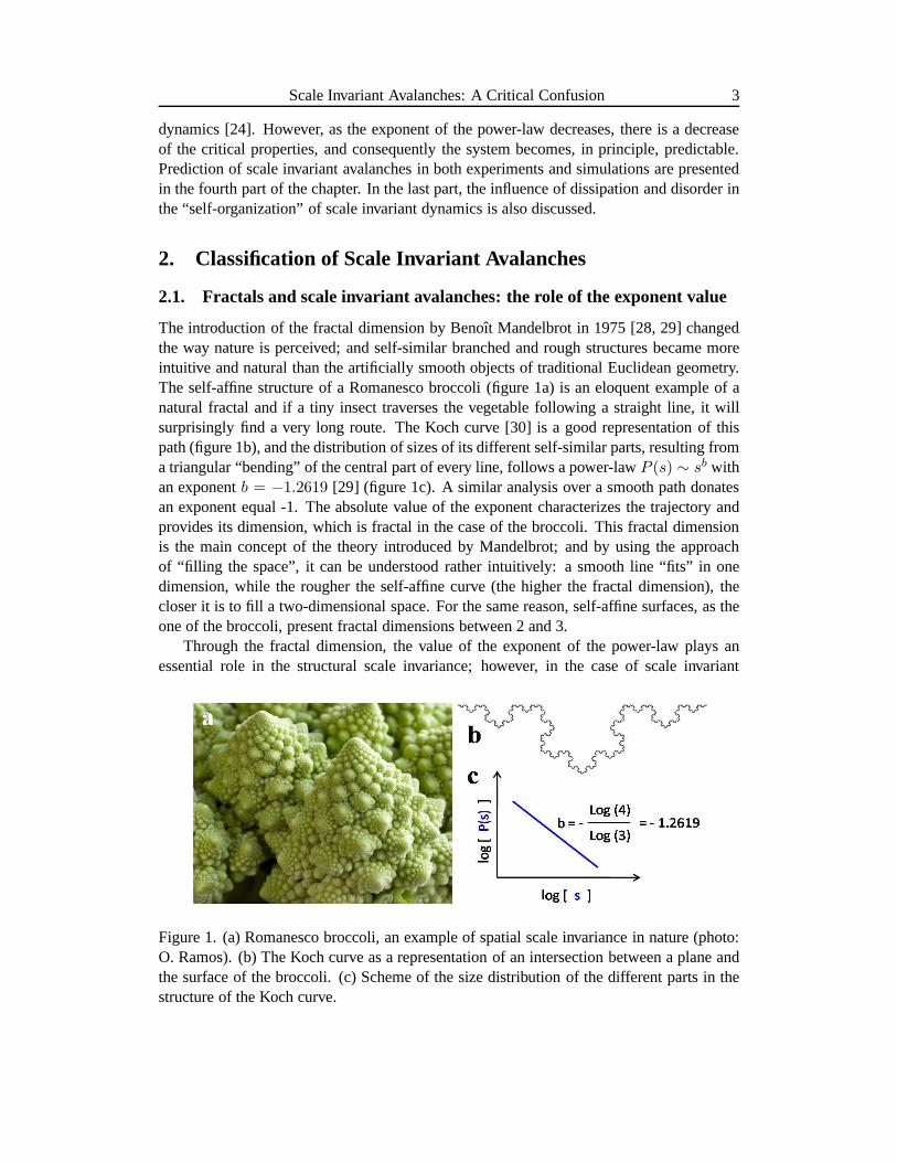
The introduction of the fractal dimension by Benoıt Mandelbrot in 1975 [28, 29] changedthe way nature is perceived; and self-similar branched and rough structures became moreintuitive and natural than the artificially smooth objects of traditional Euclidean geometry.The self-affine structure of a Romanesco broccoli (figure 1a)is an eloquent example of anatural fractal and if a tiny insect traverses the vegetablefollowing a straight line, it willsurprisingly find a very long route. The Koch curve [30] is a good representation of thispath (figure 1b), and the distribution of sizes of its different self-similar parts, resulting froma triangular “bending” of the central part of every line, follows a power-lawP (s) ∼ sb withan exponentb = −1.2619 [29] (figure 1c). A similar analysis over a smooth path donatesan exponent equal -1. The absolute value of the exponent characterizes the trajectory andprovides its dimension, which is fractal in the case of the broccoli. This fractal dimensionis the main concept of the theory introduced by Mandelbrot; and by using the approachof “filling the space”, it can be understood rather intuitively: a smooth line “fits” in onedimension, while the rougher the self-affine curve (the higher the fractal dimension), thecloser it is to fill a two-dimensional space. For the same reason, self-affine surfaces, as theone of the broccoli, present fractal dimensions between 2 and 3.
Through the fractal dimension, the value of the exponent of the power-law plays anessential role in the structural scale invariance; however, in the case of scale invariant
Figure 1. (a) Romanesco broccoli, an example of spatial scale invariance in nature (photo:O. Ramos). (b) The Koch curve as a representation of an intersection between a plane andthe surface of the broccoli. (c) Scheme of the size distribution of the different parts in thestructure of the Koch curve.
4 O. Ramos
avalanches, the relevance of the exponent is much less understood. The earthquake dy-namics is the phenomenon that normally comes to people’s minds as the example of scaleinvariance in the temporal domain. Regardless the value of the exponent of the power-lawdistribution, the interpretation of scale invariance is limited to the absence of characteristicavalanches, and the existence of many small events and a few very large ones. Temporal re-lations between events are sometimes wrongly added to the interpretation, considering thatthere is no correlation between the different avalanches. The logarithmic scale in whichthe Gutenberg-Richter law was originally introduced [31] has also created confusion in thevalue of the exponent for the distribution of earthquakes, and consequently the implicationsof this value in the dynamics of scale invariant avalanches.Further down two examples withdifferent exponents will clarify that, as in the case of fractal structures, the exponent of thepower-law distributiondoesplay a central role in the dynamics of scale invariant avalanches.However, first we will analyze how to classify scale invariant phenomena, where the his-torical use of a logarithmic scale has added some confusion to the interpretation of scaleinvariant avalanches.
2.2. The origin of logarithmic scales
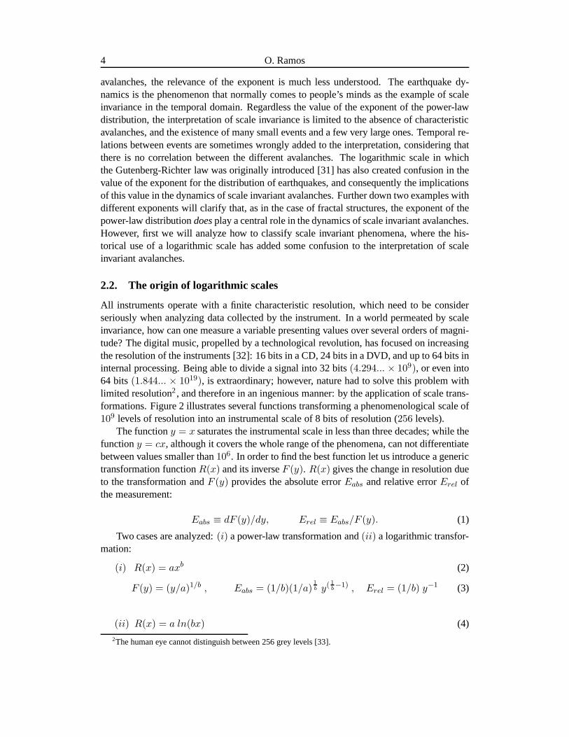
All instruments operate with a finite characteristic resolution, which need to be considerseriously when analyzing data collected by the instrument.In a world permeated by scaleinvariance, how can one measure a variable presenting values over several orders of magni-tude? The digital music, propelled by a technological revolution, has focused on increasingthe resolution of the instruments [32]: 16 bits in a CD, 24 bits in a DVD, and up to 64 bits ininternal processing. Being able to divide a signal into 32 bits (4.294... × 109), or even into64 bits(1.844... × 1019), is extraordinary; however, nature had to solve this problem withlimited resolution2, and therefore in an ingenious manner: by the application ofscale trans-formations. Figure 2 illustrates several functions transforming a phenomenological scale of109 levels of resolution into an instrumental scale of 8 bits of resolution (256 levels).
The functiony = x saturates the instrumental scale in less than three decades; while thefunctiony = cx, although it covers the whole range of the phenomena, can notdifferentiatebetween values smaller than106. In order to find the best function let us introduce a generictransformation functionR(x) and its inverseF (y). R(x) gives the change in resolution dueto the transformation andF (y) provides the absolute errorEabs and relative errorErel ofthe measurement:
Eabs ≡ dF (y)/dy, Erel ≡ Eabs/F (y). (1)
Two cases are analyzed:(i) a power-law transformation and(ii) a logarithmic transfor-mation:
(i) R(x) = axb (2)
F (y) = (y/a)1/b , Eabs = (1/b)(1/a)1
b y(1
b−1) , Erel = (1/b) y−1 (3)
(ii) R(x) = a ln(bx) (4)
2The human eye cannot distinguish between 256 grey levels [33].
Scale Invariant Avalanches: A Critical Confusion 5
F (y) = (1/b) exp(y/a) , Eabs = (1/ab) exp(y/a) , Erel = 1/a (5)
In the case of the power-law transformation, the absolute error depends on the valueof the exponent. Forb = 1 (linear case)Eabs is constant, forb > 1 it decreases with themeasured value, thus the larger the value the more accurate the measurement. Forb < 1,the absolute error increases with the measured value. If a phenomenon occurs over severalorders of magnitude, only the caseb < 1 can fulfil an instrumental scale with limitedresolution. In the three cases the relative error decreaseswith the measured value. As aconsequence, in the situation of a fractal structure as the one presented in figure 1; thelarger the measured field, the larger the number of sublevelsresolved by the measurement.Following this reasoning, if a digital camera is used as the instrument of measurement,as the camera moves apart in order to capture a larger structure, the number of pixels ofthe camera have to increase, a situation that is normal and common when one uses a tapemeasure: in order to measure a larger structure, the tape is enlarged and the number ofunits of measurement increase; thus the relative error decreases. This effect introducesa scale during the process of measurement, and allows knowing the size of the structurethrough the analysis of the relative error; thus, a power-law transformation “breaks” thescale invariance. However, the logarithmic transformation keeps constant the relative error.By using the same example, the resolution of the camera does not change when the cameramoves apart, and there are no differences between two imagestaken at different scales. Inthis sense a logarithmic transformation respects the scaleinvariance, and this is the mainreason for using this scale transformation in the classification of scale invariant phenomena.
Another reason is historical. In 1856 the English astronomer Norman R. Pogson pro-posed the current form of classification of the stars in different magnitudes in relation to thelogarithm of their brightness [34]. He based the system on the work of Ptolemy [35], whoprobably based his work on the writings of the ancient Greek astronomer Hipparchus [36].In 1860 the experimental psychologist Gustav T. Fechner proposed a logarithmic relation
100 101 102 103 104 105 106 107 108 109
0
50
100
150
200
250
y = cx
y = x
y = aln(x)
y (s
cale
of t
he in
stru
men
t)
x (scale of the phenomenon)
y = x
b
Figure 2. Different scale transformation from a phenomenonwith 109 levels of resolutioninto an instrumental scale of 8 bits of resolution.a = 256/ln(109); b = ln(256)/ln(109);c = 256/109.
6 O. Ramos
between the intensity of the sensation and the stimulus thatcauses it [37]; so the thoughtlogarithmic response of the human eye3 was responsible for the logarithmic nature of thestellar scale. In 1935 Charles F. Richter and Beno Gutenbergproposed a logarithmic scaleto describe the earthquake’s strength [39]. The name magnitude for this measurement camefrom Richter’s childhood interest in Astronomy [40]; and the scale matches in some degreethe earlier Mercalli intensity scale [41], which quantifiedthe effects of an earthquake basedon human perception.
2.3. Classifying scale invariant avalanches
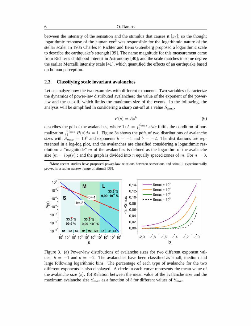
Let us analyze now the two examples with different exponents. Two variables characterizethe dynamics of power-law distributed avalanches: the value of the exponent of the power-law and the cut-off, which limits the maximum size of the events. In the following, theanalysis will be simplified in considering a sharp cut-off ata valueSmax.
P (s) = Asb (6)
describes the pdf of the avalanches, where1/A =∫ Smax
1 sbds fulfils the condition of nor-malization
∫ Smax
1 P (s)ds = 1. Figure 3a shows the pdfs of two distributions of avalanchesizes withSmax = 109 and exponentsb = −1 andb = −2. The distributions are rep-resented in a log-log plot, and the avalanches are classifiedconsidering a logarithmic res-olution: a “magnitude”m of the avalanches is defined as the logarithm of the avalanchesize[m = log(s)]; and the graph is divided inton equally spaced zones ofm. Forn = 3,
3More recent studies have proposed power-law relations between sensations and stimuli, experimentallyproved in a rather narrow range of stimuli [38].
-2,0 -1,8 -1,6 -1,4 -1,2 -1,0
0,00
0,02
0,04
0,06
0,08
0,10
0,12
0,14
100 101 102 103 104 105 106 107 108 109
10-18
10-15
10-12
10-9
10-6
10-3
100
<s>/Sm
ax
b
Smax = 103 Smax = 104 Smax = 106 Smax = 109
M1 M2 M3S3S2S1
b=-1 9,99 10-5 %
L3L2
99,9 % 9,99 10-2 %
33,3 %
33,3 %
LM
P(s)
s
S
33,3 %
L1
b=-2
Figure 3. (a) Power-law distributions of avalanche sizes for two different exponent val-ues: b = −1 and b = −2. The avalanches have been classified as small, medium andlarge following logarithmic bins. The percentage of each type of avalanche for the twodifferent exponents is also displayed. A circle in each curve represents the mean value ofthe avalanche size〈s〉. (b) Relation between the mean value of the avalanche size and themaximum avalanche sizeSmax as a function ofb for different values ofSmax.
Scale Invariant Avalanches: A Critical Confusion 7
avalanches smaller thanm = 3 are considered small(S), those lying betweenm = 3 andm = 6 are medium(M), and those greater thanm = 6 are large(L).
2.3.1. Integrated probability
The main confusion related to the logarithmic scale is a consequence of the fact that dur-ing the measurement, an integration has been already performed, which is well describedthrough the integrated probability:PInt(s, k) =
∫ kss As′bds calculates the probability of
having an avalanche with size in the interval betweens andks. Due to the properties of theintegral, the integrated probability is also a power-law with an exponentb+ 1.
PInt(s, k) =ln(ks)− ln(s)
ln(Smax)=
ln(k)
ln(Smax), b = −1 (7)
PInt(s, k) =(kb+1 − 1)sb+1
(Sb+1max − 1)
≃ (1− kb+1)sb+1 , − 2 ≤ b < −1 (8)
The calculations performed with a value ofk = 103 give the probabilities of the S, Mand L avalanches shown in the graph of figure 3a. Forb = −1 the integrated probabilityis constant and equal to1/n, so the three types of avalanches have the same probabilityequal to1/3. In the same manner, consideringk = 10, the graph can be divided intodecades: 9 zones equispaced inm that can be denominated as S1, S2, S3, M1, M2, M3,and L1, L2, L3 (shown in the graph), all of them with equal probability 1/9. This situation,which evidently results from the logarithmic scale of measurement, is very far from thecommon interpretation of many small events and only a few very large ones; and in orderto illustrate it more clearly, let us imagine the scenario ofthe distribution of earthquakeswith an exponent equal to−1: the consideration that one earthquake is happening everysecond gives in average one earthquake of magnitude between2 and 3 (S3 in our scale)every9th second, but also a catastrophic quake of magnitude between 8and 9 (L3 in ourscale) every9th second. Fortunately, many real phenomena with catastrophic consequenceshave smaller exponents in their pdfs.
For b = −2, PInt(s, k) = (1 − k−1)/s. Every decade the probability decreases bya factor 10. As a consequence, the probabilities of having a small avalanche is0.999;9.99 × 10⁻⁵ for a medium size avalanche; and only9.99 × 10−7 for a large event (figure3a). Again, if we imagine the scenario of the distribution ofearthquakes with an exponentequal to−2: the consideration that one earthquake is happening every second gives onaverage one minor earthquake of magnitude between 2 and 3 (S3in our scale) every111seconds, one moderate of magnitude between 5 and 6 (M3 in our scale) every1.11 × 105
seconds (30,8 hours), and a catastrophic quake of magnitudebetween 8 and 9 (L3 in ourscale) every1.11 × 108 seconds (3,5 years).
2.3.2. Mean value of avalanche size
Another relevant quantity signaling the key role of the exponent of the power-law, corre-sponds to the mean value of the size distribution of the avalanches〈s〉 =
∫ Smax
1 sP (s)ds.
〈s〉 =Smax − 1
ln(Smax), b = −1 (9)
8 O. Ramos
〈s〉 =(b+ 1)
(b+ 2)
S(b+2)max − 1
S(b+1)max − 1
, − 2 < b < −1 (10)
〈s〉 =ln(Smax)
1− S−1max
, b = −2 (11)
The mean value of the avalanche size is related to both the response of the system to aperturbation, and the energy balance in the dynamics. In thefigure 3a, whereSmax = 109,the values of〈s〉 correspond to4.8 × 107 and20.7 for b = −1 andb = −2 respectively.These values are represented by a circle in each curve.
The value of〈s〉 corresponds to the average response of the system to a perturbation,under the consideration that small perturbations can provoke the overcoming of local thresh-olds and thus the triggering of avalanches. In average, the system is delivering an avalancheof size〈s〉; so in terms of avalanche production, this is equivalent to generate an avalancheof size 〈s〉 in every event of the dynamics. In the particular case of〈s〉 proportional tothe system size, the situation can be interpreted as critical: in average a perturbation pro-vokes a response proportional to the system size. However, the fact that the dimension ofthe avalanche is smaller than the dimension of the system, adds some complexity to theanalysis of the criticality through the avalanche size distribution, which will be discussed insection 4.1.1.
2.3.3. Energy balance in slowly driven systems
As mentioned in the introduction, avalanches are defined as sudden liberation of energythat has been accumulated very slowly. This indicates that the energy is injected in smallportions, and that there is a separation between the drive ofthe system (slow) and theavalanche duration (rapid). At every single time interval,it is possible to define an injectedenergy, an avalanche of a particular size, and a dissipated energy. If the system is in astationary state, the average energy injected to the systemin every time interval has to beequal to the average dissipated energy. Consequently, the average dissipated energy has tobe small,
〈Einjected〉 = 〈Edissip〉. (12)
Many of the models dealing with scale invariant avalanches are non-dissipative in thebulk, and the energy is liberated through the boundaries of the system [22]. However, theystill refer as avalanches the local processes related to rearrangements in the bulk of thesystem, with no energy cost. As the avalanche production is not directly related to thedissipation of energy, these systems can have a large value of 〈s〉 and still present a smallaverage value of the dissipated energy〈Edissip〉.
However, the vast majority of real phenomena are dissipative. Considering that
〈Einjected〉 ∼ Smin << Smax, and 〈Edissip〉 = α〈s〉, (13)
whereα is a dissipation coefficient,
α〈s〉 << Smax. (14)
Scale Invariant Avalanches: A Critical Confusion 9
The larger the avalanche size, the larger the dissipation; and as a consequence, largevalues of〈s〉 are forbidden for dissipative slowly driven system. Figure3b shows the re-lation 〈s〉/Smax for different b values, indicating that large values ofb (close to−1) areforbidden for dissipative slowly driven system.
The previous analysis did not consider the existence of avalanches of size zero (let uscall themzeroavalanches), where the addition of energy to the system provokes no responsein terms of avalanches (s < Smin). In order to compensate the energy lost for an averagenon-zeroavalanche〈s〉, the system needs a numbernS0 of zeroavalanches proportional toα〈s〉/Smin. For smallb values, and thus smallα〈s〉, nS0 can be the consequence of a lackof resolution in the measurement.
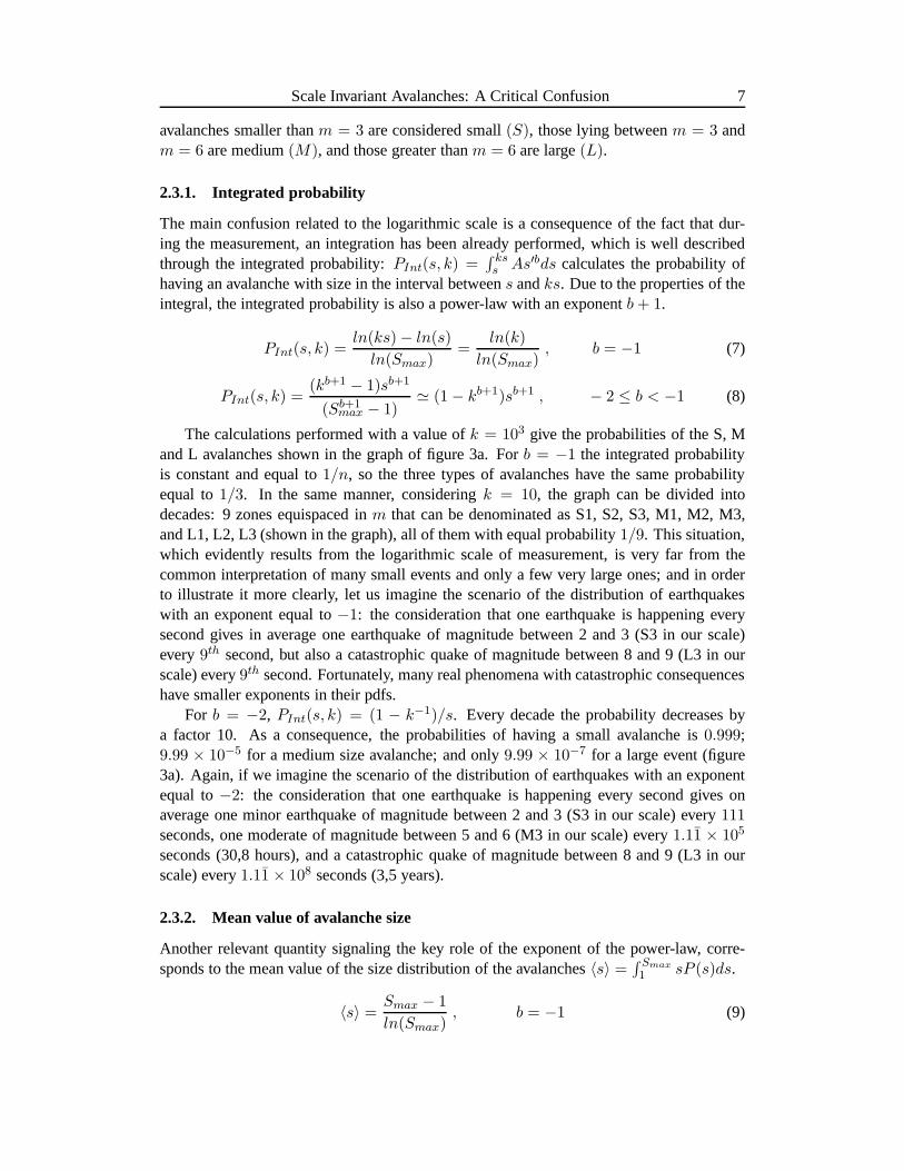
2.3.4. The distribution of earthquakes
The Gutenberg-Richter law [31] is the best known example of scale invariant avalanches.However, many studies from the Statistical Physics point ofview have not considered thefact that the original distribution was measured in a logarithmic scale, which provokes achange equal -1 in the measured exponent [2, 42]. Other reports attribute this change to acumulative manner in the definition of the probability [43],which is mathematically correct,but it is not the right interpretation; and it brings confusion to the Geological community[44].
2 3 4 5 6 7 8 9
100
101
102
103
104
105
106
Freq
uenc
y (E
arth
quak
es /
year
)
Magnitude
A B C PInt(1s) PInt(0,21s)
s=-1
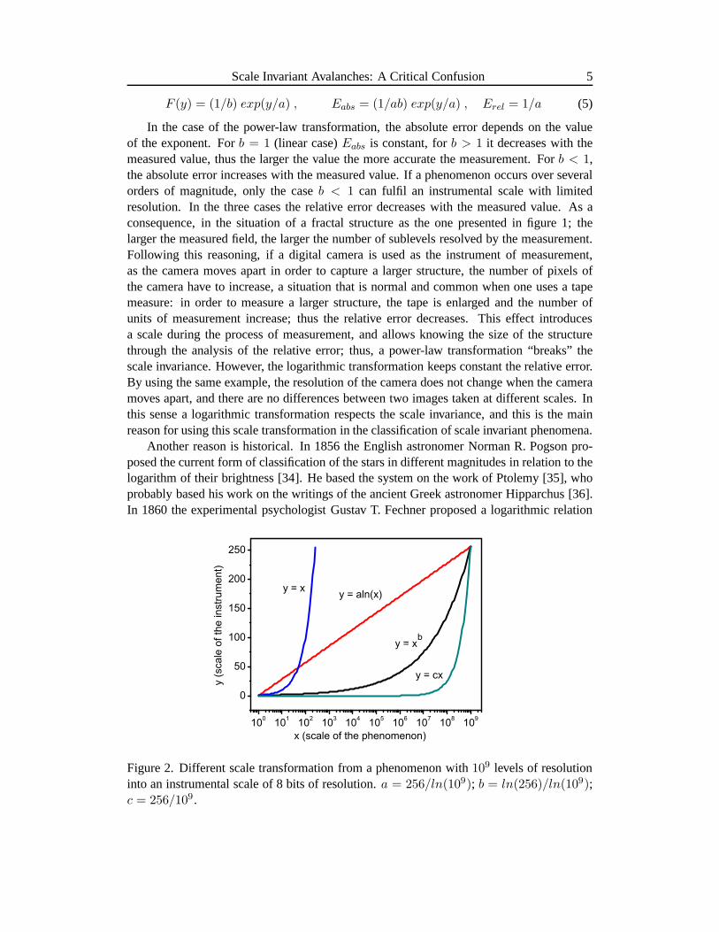
Figure 4. Frequency of earthquake occurrence worldwide. Data from the U.S. GeologicalSurvey [45]: (A) Based on observations since 1900. (B) Basedon observations since 1990.(C) Estimated. A solid line with slopes = −1 serves a a guide. The solutions of theIntegrated probability forb = −2, considering that one earthquake occurs every second,and every 0.21 seconds, are also displayed.
Figure 4 displays the frequency of earthquake occurrence worldwide. The fact that theresults are presented in intervals of magnitude indicates that the distribution corresponds tothe integrated probabilityPInt(ML), whereML is the local magnitude. The graph showsthat log[Pint(ML)] ∼ −ML. By substitutingML into the definitions

10 O. Ramos
ML ≡ log(A) + const (15)
ML ≡ 2/3 log(E) + const (16)
whereA (wave amplitude) is the maximum excursion of the Wood-Anderson seismograph,according to the original work of Richter [39], andE the energy released by a quake, onegetsPInt(AL, 10) ∼ A−1 andPInt(EL, 10) ∼ E−2/3. By adding−1 to the values of theexponents in the integrated probability, as discussed earlier (section 2.3.1.), it is possible toobtain the distributions of earthquakes in terms ofA andE:
P (A) ∼ A−2, P (E) ∼ E−5/3 (17)
In order to illustrate the integrated probability for the distributions of figure 3 (sec-tion 2.3.1.), the consideration of one earthquake happening every second was used. Theresults of this assumption for the caseb = −2 are plotted in figure 4, and they are a lit-tle lower than the real values. However, the same analysis under the consideration of oneearthquake occurring every0.21 seconds fits quite well the real data (figure 4).
3. Avalanches in Critical Phenomena
The original motivation of this section was to study the properties of the scale invariantavalanches in well established critical systems, in order to compare them with the SOCavalanches. As discussed in the introduction, the SOC borrowed the concept of criticalpoint of equilibrium phase transitions in order to describetheir uncorrelated power-law dis-tributed avalanches. The termcritical in the avalanche context has been presented throughthe fact that at any moment a minor perturbation can trigger aresponse (avalanche) of anysize and duration, a behavior that is linked to a divergence of the correlation length in theoriginal numerical model of SOC: the BTW model [22]. Many dissipative phenomena in-volving avalanches distributed according to power-laws have been treated as critical systems[23, 24]; however, recent studies have shown different systems evolving through power-lawdistributed avalanches in a non-critical behavior [12, 46,47], which has motivated the anal-ysis of the avalanche dynamics in a well established critical scenario: a second order phasetransition.
In Physics, the classical scenario of critical phenomena takes place during a second or-der phase transition [48]. The text-book example is the transition where a permanent magnetloses its magnetism: its magnetic properties cease when thetemperature is increased abovea certain critical temperatureTc. Below this temperature, a majority of spins point in thesame direction, creating a magnetic field. Large fluctuations in spins do not occur at lowtemperatures, thus the system will remain unchanged. Abovethe critical temperature thespins’ directions are random and change direction randomly, frequently and individually.The system is already disordered, therefore, no large-scale changes will happen; there is nooverall magnetic field. However, at the critical temperature itself, large fluctuations occurand different snapshots of the system show different patterns - but all of the patterns willbe statistically similar, in that clusters of aligned spinsare surrounded by areas with spinsoriented in the opposite direction. The clusters are of all sizes and their distribution follows
Scale Invariant Avalanches: A Critical Confusion 11
a power-law [49]. Four characteristic of this critical state will be used in our analysis alongthis chapter:
a) Divergence of the correlation length (ξ): The temporal average of the spatial auto-correlation function
〈CAs(d, t)〉t =
⟨
∑
f(x, y)f(x′, y′)− 〈f(x, y)〉2∑
(f(x, y)− 〈f(x, y)〉)2
⟩
t
(18)
wheref(x, y) represents the structure of the system (in two dimensions) andd correspondsto the distance between(x, y) and(x′, y′), can generally be fitted (∀T 6= Tc) as an expo-nential decay in the form
〈CAs(d, t)〉t ∼ exp(−d/ξ). (19)
At the critical point, the correlation lengthξ is proportional to the linear size of thesystemL (diverging in an infinite system). The temporal average is necessary because thecalculus is performed in a snapshot of the dynamics (a microstate), and any physical mea-sure implies an average over many different microstates, which is equivalent to a temporalaverage if the system is ergodic [50].
b) Divergence of the correlation time (τ ): The temporal autocorrelation function
CAt(t) =
∑
f(ti)f(ti + t)− 〈f(ti)〉2
∑
(f(ti)− 〈f(ti)〉)2(20)
can be fitted as an exponential decay in the form
CAt(t) ∼ exp(−t/τ). (21)
Far from the critical point, the correlation timeτ is small, so the system will quicklyrecover from a perturbation. At the critical point,τ diverges due to the fact that the systemhesitates between the two states, and perturbations can move the system away from itsequilibrium state during long periods of time. As a result, the dynamics turns slow, aphenomenon which is known ascritical slowing down(CSD) [50].
c) Both ξ andτ present power-law dependencies with the reduced temperature Tr =(T − Tc)/Tc in the wayξ = |Tr|
−ν andτ = |Tr|−zν ; and thus they relate to each other
throughτ = ξz. ν is called acritical exponentand is an attribute of the Ising model.Phenomena with the same critical exponents belong to the same universality class. Theexponentz is often called the dynamic exponent. It gives a way to quantify the CSD and itdepends on the algorithm, i.e., it depends on the type of dynamics [50].
d) As the size of the system increases, the transition between the two states becomessharper, and it is infinitely sharp in an infinite system [50].
3.1. Avalanches6= fluctuations
3.1.1. Simulation: the Ising model
In this subsection, the dynamics of avalanches is studied ina well established critical sys-tem: the Ising model, which is certainly the most thoroughlyresearched model in the whole
12 O. Ramos
of statistical physics. It is a model of a magnet, and consists of a lattice where every siterepresents a spin of unit magnitude taking two values±1 as an indication of the only twopossible directions to point: “up” or “down”. The spins interact with their nearest neigh-bors and the magnetizationM is the sum over all the spins. For two or more dimensionsthe system shows a second order phase transition at a critical temperatureTc (Tc = 2.269in two dimensions) from a ferromagnetic to a paramagnetic state when the temperature isincreased, and in two dimensions the model is analytically solved [51]. The behavior ofthe average fluctuations of the magnetization is well known,and it defines the magneticsusceptibility, as well as its relation with the correlation function. The fluctuations of themagnetization (M − 〈M〉) have also been studied [52], and their pdf is reported to be uni-versal [53]. It presents an exponential tail on one side, anda rapid falloff on the other side.However, in the scenario of SOC systems, instead of analyzing the fluctuations of the mag-nitudes, the standard is to define avalanches, corresponding to relative differences betweenconsecutive states. Therefore, the definition of avalanches presented in the introduction,which is relative to slowly driven system, has been extendedto differences between equi-spaced values in the time series of the measured variable. In the case of the Ising model,they corresponds to jumps in the magnetization between two consecutive microstates. Smallsimulations, both in size and in running time, will be sufficient to illustrate the dynamics ofavalanches in this critical scenario.
The simulations take place in a128 × 128 lattice with periodic boundary conditions,and compute106 Monte Carlo steps (MCS) after105 thermalization steps. Both Metropolis[55] and Wolff [56] algorithms are implemented consideringno external magnetic field.Thus the energy of the system reads asE = −J
∑N〈i,j〉 sisj whereJ = 1 is a coupling
constant and〈i, j〉 indicates that the sum is over nearest neighbors only. In theMetropolisalgorithm one MCS consists ofN = (128)2 events where one random spin is selected, andflipped (si = −si) if exp(−∆E/KT ) is larger or equal to a random number between 0 and1. ∆E is the change in energy due to the flip of the spin, and K is considered equal to 1, sothe temperature T is presented as an adimensional magnitude. In the Wolff algorithm, one
1,8 2,0 2,2 2,4 2,6 2,8
0,0
0,2
0,4
0,6
0,8
1,0
0
2
4
6
8
10
|m| Wolff |m| Met.
|m|
T
Wolff Met.
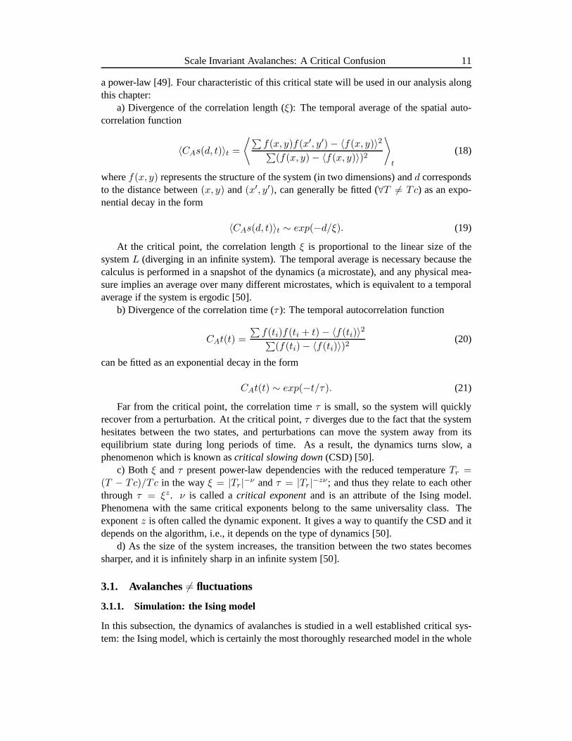
Figure 5. Average of the absolute value of the magnetizationper spin and correlation lengthfor both Metropolis and Wolff algorithms at different temperatures.
Scale Invariant Avalanches: A Critical Confusion 13
MCS consists of building up a cluster of flipped spins. Starting from flipping one spin at arandom position, its neighbors will become part of the growing cluster ifexp(−2J/KT ) issmaller than a random number between 0 and 1.
The average of the absolute value of the magnetization per spin m, and the value ofthe correlation lengthξ are shown in figure 5. The correlation length has been extractedfollowing the eqs. 18 and 19:
〈C(r)〉t =
⟨ ∑Nd(i,j)=r(sisj)−m2
∑Nd(i,j)=r(si|sj| −m)2
⟩
t
(22)
〈C(r)〉t ∼ exp(−r/ξ). (23)
The correlation function has been calculated by using periodic boundary conditions,through an average of values taken every thousand MCS, and the sum is over those sitesthat are separated from each other by a distance equal tor. Both algorithms give verysimilar results on the averages of the physical magnitudes,with a peak in the correlationlength coinciding with the phase transition.
The behavior of the fluctuations for the Wolf algorithm is presented in figure 6. Forvery low temperatures two symmetric Gaussian distributions (GDs) in the pdf of the mag-netization indicate the two symmetric ordered states in thesystem (not shown in the graph).
-0,1 0,0 0,1
0
8k
16k
24k
32k
-0,8 -0,4 0,0 0,4
0
2k
4k
6k
8k
-0,8 -0,4 0,0 0,4 0,80
2k
4k
6k
-0,8 -0,4 0,0 0,4 0,8
0
4k
8k
12k
16k
-0,2 0,0 0,2
0
4k
8k
12k
16k
-0,2 0,0 0,2
0
4k
8k
12k
16kd
T=2,2
e
b
T=2,6Tc=2,269
PD
F
m-<m>|m|-<|m|>|m|-<|m|>
mm
PD
F
m
a c
f
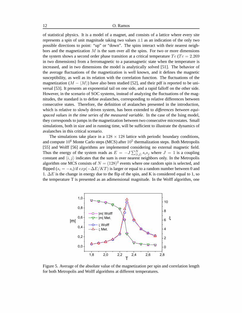
Figure 6. (a-c) Distribution of the magnetization for the Wolff algorithm at different temper-atures. At the critical point, the distribution for the Metropolis algorithm is also displayed(b), presenting an asymmetric behavior. (d, e) Distribution of the fluctuations of the absolutevalue of the magnetization for the Wolf algorithm at different temperatures. (f) Distributionof the fluctuations of the magnetization for the Wolff algorithm at T=2.6.
14 O. Ramos
As the temperature increases, the two GDs approach each other (figure 6a) and a smallasymmetry starts to be noticed at the low frequencies in the pdf of the fluctuations of theabsolute value of the magnetization (figure 6d). At the critical point, the two GDs start tomerge forming the universal Gumbel distribution reporter by Bramwellet. al. in the pdf ofthe fluctuations of the absolute value of the magnetization [53, 54] (figure 6e). This Gumbeldistribution of the fluctuations has been used by different experiments as an indication ofthe criticality of the system [57, 58]. For high temperatures we can considerthat the twoGDs have perfectly merged, and there is a Gaussian behavior of the fluctuation of the mag-netization (figure 6f). In the case of the Metropolis algorithm only one side of the graph (a)will be explored by the system in a finite time (either positive or negative magnetization).The asymmetry displayed by the Metropolis algorithm in the graph (b) is a consequence ofits slow dynamics, as it will be discussed further down.106 MCS are not enough for thesystem to spend on average the same “time” in symmetrical areas of the phase space (with107 MCS both algorithms have given the same result). The other graphs (c−f ) are the samefor both algorithms; consequently, they give the same results concerning the fluctuations ofthe absolute value of the magnetization.
0 2000 4000 60000
2k
4k
6k
8k
-400 -200 0 2000
6k
12k
18k
Number of flips
T=1.8
T=2.2
T=2.269
T=2.3 T=2.7
b
T=2.269PD
F
Size of the avalanches
T=1.8
T=2.2
T=2.3
T=2.7
a
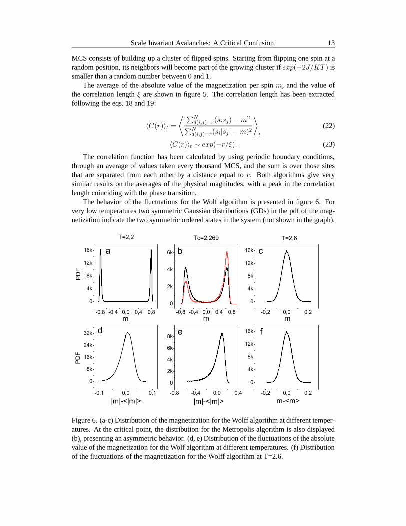
Figure 7. a) Distribution of the jumps in the magnetization (avalanches) for different tem-peratures (T) with the Metropolis algorithm. The curves correspond to T values between1.8 and 2.7 with spacings of 0.1, and also the critical point:Tc = 2.269. b) Distributions offlips for different temperatures.
The distributions of the jumps ofM (avalanches) and the distributions of flips for theMetropolis algorithm are displayed in figure 7. The avalanches follow a Gaussian for everymeasured T, and the distributions widen as T increases (figure 7a). The distributions of flips(figure 7b) also follow Gaussian distributions, with their mean values increasing with T andstandard deviations having a maximum at the critical valueTc = 2.269.
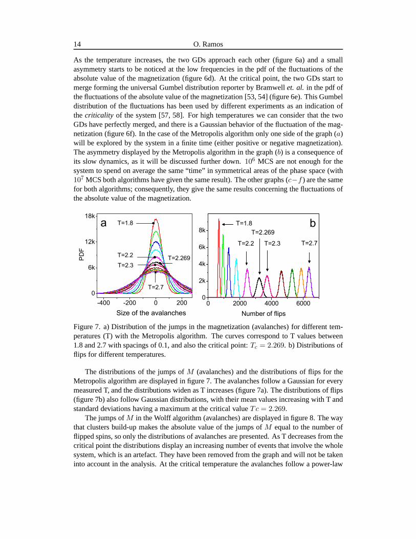
The jumps ofM in the Wolff algorithm (avalanches) are displayed in figure 8. The waythat clusters build-up makes the absolute value of the jumpsof M equal to the number offlipped spins, so only the distributions of avalanches are presented. As T decreases from thecritical point the distributions display an increasing number of events that involve the wholesystem, which is an artefact. They have been removed from thegraph and will not be takeninto account in the analysis. At the critical temperature the avalanches follow a power-law
Scale Invariant Avalanches: A Critical Confusion 15
100 101 102 103 104
10-1
100
101
102
103
104
105
100 101 102 103 104
100
101
102
103
104
105
b
Tc=2,269 T=2,3 T=2,4 T=2,5 T=2,6 T=2,7
Size of the avalanches
Tc=2,269 T=2,2 T=2,1 T=2,0 T=1,9 T=1,8
PD
F
Size of the avalanches
b=-1,1
a
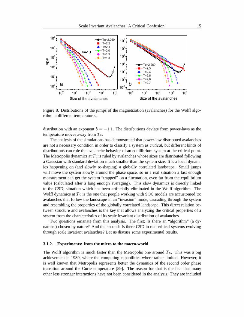
Figure 8. Distributions of the jumps of the magnetization (avalanches) for the Wolff algo-rithm at different temperatures.
distribution with an exponentb = −1.1. The distributions deviate from power-laws as thetemperature moves away fromTc.
The analysis of the simulations has demonstrated that power-law distributed avalanchesare not a necessary condition in order to classify a system ascritical, but different kinds ofdistributions can rule the avalanche behavior of an equilibrium system at the critical point.The Metropolis dynamics atTc is ruled by avalanches whose sizes are distributed followinga Gaussian with standard deviation much smaller than the system size. It is a local dynam-ics happening on (and slowly re-shaping) a globally correlated landscape. Small jumpswill move the system slowly around the phase space, so in a real situation a fast enoughmeasurement can get the system “trapped” on a fluctuation, even far from the equilibriumvalue (calculated after a long enough averaging). This slowdynamics is directly linkedto the CSD, situation which has been artificially eliminatedin the Wolff algorithm. TheWolff dynamics atTc is the one that people working with SOC models are accustomedto:avalanches that follow the landscape in an “invasion” mode,cascading through the systemand resembling the properties of the globally correlated landscape. This direct relation be-tween structure and avalanches is the key that allows analyzing the critical properties of asystem from the characteristics of its scale invariant distribution of avalanches.
Two questions emanate from this analysis. The first: Is therean “algorithm” (a dy-namics) chosen by nature? And the second: Is there CSD in realcritical systems evolvingthrough scale invariant avalanches? Let us discuss some experimental results.
3.1.2. Experiments: from the micro to the macro-world
The Wolff algorithm is much faster than the Metropolis one aroundTc. This was a bigachievement in 1989, where the computing capabilities where rather limited. However, itis well known that Metropolis represents better the dynamics of the second order phasetransition around the Curie temperature [59]. The reason for that is the fact that manyother less stronger interactions have not been considered in the analysis. They are included

16 O. Ramos
-10 -5 0 51
10
100
1k
10k
-10 -5 0 5 10
0
1k
2k
3k
4k
-10 -5 0 5
0
1k
2k
3k
4k
5k
P-<P>
b
=1 =2 =3 =5 =10 =100
P(t)-P(t+ )
PD
F
P-<P>
a
Figure 9. a) Distribution of the fluctuations of the total power injected to the motors of therotatory disks in a turbulent flow experiment. Inset: The same function in log-lin axes, inorder to enhance the asymmetry of the Gumbel. b) Distributions of avalanches for differentτ values.
in something denominatedthermal bathwhich tries to equilibrate the dynamics. Recentexperiments have focused on the non-gaussian (Gumbel) distribution of fluctuations closeto the Freedericksz transition, a second order phase transition in a liquid crystal [57], andthey have also confirmed the Gaussian character of the avalanche distributions close to thecritical point [60]. However, if the system is kept at a low temperature (belowTc) andan external magnetic field is applied, the spins try to align themselves with the externalfield, and a reorganization of the magnetics domains takes place. This reorganization isnot a smooth process, but is composed of small bursts or avalanches distributed followinga power-law; a phenomenon which has been widely studied fromthe avalanche context[61, 62, 63] and is known as the Barkhausen effect [64].
Moving towards the macro-world, a turbulent flow is another phenomenon where non-gaussian fluctuations have been reported [54, 65]: two coaxial disks counter-rotate at a fixedvelocity generating a swirling flow in the gap between them. The power required to keepa constant velocity of the disks (through a feedback loop) ismeasured and the fluctuationsof the power correspond to the variable of analysis. If the experiment is performed insidea cylinder coaxial with the disks but with a diameter much larger than the disks’ diameter,the fluctuations of the total power follow a Gaussian distribution. However, if the diameterof the cylinder is only slightly larger than the disks’ diameter, the fluctuations of the totalpower follow a Gumbel distribution.The data presented in [54] have been reanalyzed forthis chapter (courtesy of J.-F. Pinton): avalanches have been defined as relative differencesbetween two points separated a time intervalτ in the time series of total power. Whilethe fluctuations of the total power display a Gumbel distribution (figure 9a), interpreted asa signature of a critical scenario; the avalanches follow a Gaussian distribution for all thedifferentτ values (figure 9b). A remarkable difference in relation to the Ising model is thefact that the standard deviations of the Gaussian distributions are comparable to the widthof the Gumbel. By following the same reasoning used in the Ising model, the Gumbel canbe explained as the merging of the two Gaussian distributions of the fluctuations of theindividual disks due to the confinement, which reduces the number of degrees of freedom
Scale Invariant Avalanches: A Critical Confusion 17
−5 0 5 10
10−4
10−2
100
Y=(V−⟨V⟩)/σ
P(Y
)
10−1
100
101
10−2
10−1
100
101
P(S
/⟨S⟩)
S/⟨S⟩
v=0.057mm/sv=0.094mm/sv=0.134mm/sv=0.185mm/sv=0.225mm/s
P∝ X−αe−X/ξS
α=1.00 ± 0.06ξ
S=4.3 ± 1.4
ba
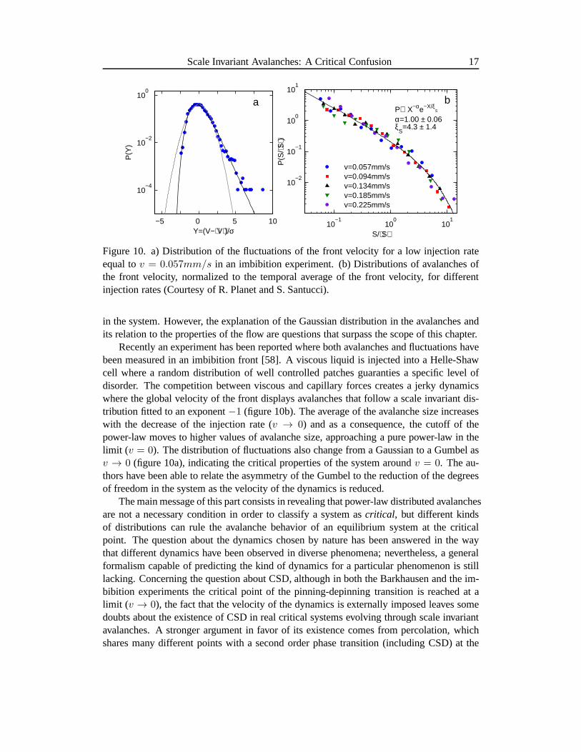
Figure 10. a) Distribution of the fluctuations of the front velocity for a low injection rateequal tov = 0.057mm/s in an imbibition experiment. (b) Distributions of avalanches ofthe front velocity, normalized to the temporal average of the front velocity, for differentinjection rates (Courtesy of R. Planet and S. Santucci).
in the system. However, the explanation of the Gaussian distribution in the avalanches andits relation to the properties of the flow are questions that surpass the scope of this chapter.
Recently an experiment has been reported where both avalanches and fluctuations havebeen measured in an imbibition front [58]. A viscous liquid is injected into a Helle-Shawcell where a random distribution of well controlled patchesguaranties a specific level ofdisorder. The competition between viscous and capillary forces creates a jerky dynamicswhere the global velocity of the front displays avalanches that follow a scale invariant dis-tribution fitted to an exponent−1 (figure 10b). The average of the avalanche size increaseswith the decrease of the injection rate (v → 0) and as a consequence, the cutoff of thepower-law moves to higher values of avalanche size, approaching a pure power-law in thelimit (v = 0). The distribution of fluctuations also change from a Gaussian to a Gumbel asv → 0 (figure 10a), indicating the critical properties of the system aroundv = 0. The au-thors have been able to relate the asymmetry of the Gumbel to the reduction of the degreesof freedom in the system as the velocity of the dynamics is reduced.
The main message of this part consists in revealing that power-law distributed avalanchesare not a necessary condition in order to classify a system ascritical, but different kindsof distributions can rule the avalanche behavior of an equilibrium system at the criticalpoint. The question about the dynamics chosen by nature has been answered in the waythat different dynamics have been observed in diverse phenomena; nevertheless, a generalformalism capable of predicting the kind of dynamics for a particular phenomenon is stilllacking. Concerning the question about CSD, although in both the Barkhausen and the im-bibition experiments the critical point of the pinning-depinning transition is reached at alimit (v → 0), the fact that the velocity of the dynamics is externally imposed leaves somedoubts about the existence of CSD in real critical systems evolving through scale invariantavalanches. A stronger argument in favor of its existence comes from percolation, whichshares many different points with a second order phase transition (including CSD) at the
18 O. Ramos
percolation threshold, and where the avalanches are power-law distributed [66]. Anotherthing to retain from this part is the value of the exponent of the power-law displayed by awell established critical system in two dimensions.
4. Criticality in Scale Invariant Avalanches
4.1. Models without spatial structure
After the introduction in 1987 of the SOC [22] as a new critical phenomenon occurring ina class of dissipative coupled systems triggered by temporal fluctuations, many differentapproaches have been used in order to describe its dynamics.The first one corresponded tothecritical branching process[25].
P2
P1
P0
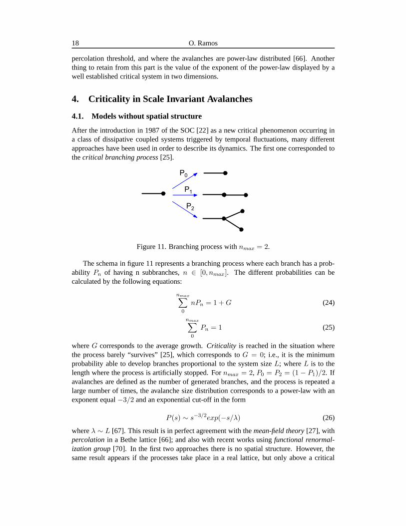
Figure 11. Branching process withnmax = 2.
The schema in figure 11 represents a branching process where each branch has a prob-ability Pn of having n subbranches,n ∈ [0, nmax]. The different probabilities can becalculated by the following equations:
nmax∑
0
nPn = 1 +G (24)
nmax∑
0
Pn = 1 (25)
whereG corresponds to the average growth.Criticality is reached in the situation wherethe process barely “survives” [25], which corresponds toG = 0; i.e., it is the minimumprobability able to develop branches proportional to the system sizeL; whereL is to thelength where the process is artificially stopped. Fornmax = 2, P0 = P2 = (1 − P1)/2. Ifavalanches are defined as the number of generated branches, and the process is repeated alarge number of times, the avalanche size distribution corresponds to a power-law with anexponent equal−3/2 and an exponential cut-off in the form
P (s) ∼ s−3/2exp(−s/λ) (26)
whereλ ∼ L [67]. This result is in perfect agreement with themean-field theory[27], withpercolationin a Bethe lattice [66]; and also with recent works usingfunctional renormal-ization group[70]. In the first two approaches there is no spatial structure. However, thesame result appears if the processes take place in a real lattice, but only above a critical
Scale Invariant Avalanches: A Critical Confusion 19
dimensiondc. The higher the dimension, the less the probability for a branch to form aloop; and this absence of loops is a necessary conditions that makes the calculation pos-sible. Unfortunately,dc = 4 for the branching process [68, 69], and for the functionalrenormalization group [70]. For percolationdc = 6 [66]. However, in real situations of twoand three dimensions the results are different, and we will find values smaller than -3/2 forthe critical exponents.
4.1.1. The role of dissipation and the structure of the avalanches
Although the solution displayed by eq. 26 works for spatial dimensions beyond the realworld, it is very useful both for setting the lower limit to the critical exponents to -3/2, andfor understanding the main concepts through discussion on an analytic base. By settinga negative value toG in eq. 24 it is possible to simulate the effect of the dissipation dur-ing the branching process: At every branching occasion, theprobability is lower than thecritical one; and as a result the average length of the branches decreases. The solution ofthe avalanche size distribution has the same shape (eq. 26),but with the difference thatλdecreases with the dissipation, results that have also beenreported in a Bethe lattice [71].Dissipation reduces the size of the avalanches, and as a consequence the linear size of themean avalanche is not proportional to the linear size of the system.λ is normally consid-ered as the correlation lengthξ, with the implication that the system is critical only in theconservative case.
There is a general belief that a dynamic of power-law distributed avalanches is a signa-ture of a critical scenario (independently of the value of the exponent), and that the existenceof a cut-off is the indication of the loose of critical properties. This consideration is basedon the fact that, regardless the value of the exponent, eventually an avalanche is reachingthe system size (st ∼ L). However, in the analysis of the correlation length in section 3.,the necessity of the temporal average has been presented. A particular avalanche (st) corre-sponds to a “microstate” in the dynamics, and a temporal average is needed in order to getthe values of the physical magnitudes. Let us analyze this indetail:
The correlation lengthξ has been defined in the eqs. 18 and 19; and thecriticality of asystem has been introduced as the divergence of the correlation length (ξ ∼ L). The anal-ysis of the Wolff algorithm in section 3.1.1. has shown a strong relation between structureand avalanche dynamics, suggesting that in a dynamics of scale invariant avalanches, it ispossible to measure thecriticality of the system through the average value of the avalanchesizes:
〈s〉1/dA ∼ L, (27)
wheredA corresponds to the fractal dimension of the avalanche in a system of dimensiondS , and volumeV ∼ LdS . From eq. 10 one gets〈s〉 ∼ Sb+2
max; therefore,
S(bc+2)/dAmax ∼ L ∼ V 1/dS ≥ S1/dS
max , (28)
(bc + 2)dS ≥ dA. (29)
A larger value of the exponentb provokes a larger value of〈s〉, and consequently itdelivers larger avalanche sizes. By following the same principle of the branching process,
20 O. Ramos
where the criticality was defined as the lower probability able to form branches reachingthe system size, it seems possible to choose the smallerbc. Consequently,
(bc + 2)dS = dA. (30)
The relation 30 links the critical exponentbc to the difference between the fractal dimen-sion of the avalanche and the dimension of the system. IfdA = dS , the critical exponent isequal to−1. In two and three dimensions, where the critical exponents in percolation [66]correspond to−187/91 + 1 = −1.05 and−1.18, respectively; the relation 30 gives thevalues ofdA = 1.9 (dS = 2) anddA = 2.46 (dS = 3), while the values presented by [66]correspond todA = 91/48 = 1.89 (dS = 2) anddA = 2.53 (dS = 3). Although for twoand three dimensions it seems to work, for the critical dimensiondS = 6, the relation givesa ratiodS/dA = 2, while the reported one is3/2 [66].
4.2. Avalanches in two and three dimensions
Above the critical dimension, different approaches have shown that the critical exponentof scale invariant avalanches corresponds to−3/2. Dissipation moves the cut-offs towardssmall avalanche size values, provoking a decrease in the mean value of avalanche sizes〈s〉,thus breaking the criticality of the system. In two and threedimensions the situation is morecomplex: there is no universality in the values of the critical exponents, and dissipation canhave different effects on the distribution, either changing the cut-off of the distribution [58]or decreasing the exponent of the power-law [1].
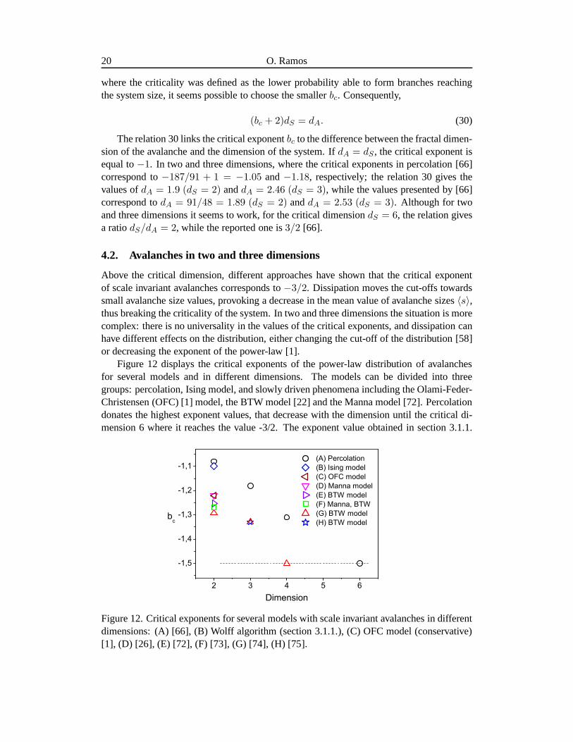
Figure 12 displays the critical exponents of the power-law distribution of avalanchesfor several models and in different dimensions. The models can be divided into threegroups: percolation, Ising model, and slowly driven phenomena including the Olami-Feder-Christensen (OFC) [1] model, the BTW model [22] and the Mannamodel [72]. Percolationdonates the highest exponent values, that decrease with thedimension until the critical di-mension 6 where it reaches the value -3/2. The exponent valueobtained in section 3.1.1.
2 3 4 5 6
-1,5
-1,4
-1,3
-1,2
-1,1 (A) Percolation (B) Ising model (C) OFC model (D) Manna model (E) BTW model (F) Manna, BTW (G) BTW model (H) BTW model
bc
Dimension
Figure 12. Critical exponents for several models with scaleinvariant avalanches in differentdimensions: (A) [66], (B) Wolff algorithm (section 3.1.1.), (C) OFC model (conservative)[1], (D) [26], (E) [72], (F) [73], (G) [74], (H) [75].
Scale Invariant Avalanches: A Critical Confusion 21
by the avalanche distribution in the Ising model (Wolff algorithm) is also displayed and itshows a value close to Percolation in two dimensions. The group of slowly driven phe-nomena in two dimensions shows values approximately in the interval (−1.3,−1.2), wherethere is also a report indicating universality with an exponent−1.27 between two of the pre-sented models [73]. For three dimensions there are much lessstudies, but some numericalresults indicate a critical exponent equal to−1.33 for the BTW model. As mentioned ear-lier, the critical dimension for slowly driven phenomena is4 [27]. Following the relation 30,the different exponents must be related to the structure of the avalanches, in particular theirfractal dimensions.
The lowest value of the critical exponent for the avalanchesin slowly driven systemscorresponds to−3/2 and takes place in dimension 4 (or superior). In three dimensionsthe results indicate a value equal to−1.33 and in two dimensions let us take−1.27 asthe paradigm. However, the majority of real phenomena evolving through scale invariantavalanches present much lower exponents: earthquakes (b = −2), granular avalanches (b =−1.6) [12], superconducting vortices (b = −1.6) [15, 16, 17, 18], solar flares (b = −1.8)[14], subcritical fracture (b = −1.5) [19], and so on. Why do these phenomena “move”apart from the critical values of their respective dimensions? Dissipation is one possibleanswer.
The Olami-Feder-Christensen (OFC) model of earthquakes isa nonconservative modelthat mimics the behavior of two tectonic plates, and is able to tune the exponent of thepower-law distribution of avalanches by modifying the degree of dissipation in the system[1]. Recent and still unpublished results in granular piles(the continuation of [12]) haveshown the same tendency displayed by the OFC model: a decrease in the value of the ex-ponent of the power-law distribution of avalanche sizes as dissipation increases. However,a quantitative relation between the dissipation and the exponent of the power-law is stilllacking. Some reports have analyzed the effect of dissipation on the critical properties inthe OFC model [76, 77, 78] and also in a more general framework[79]. The results showcritical properties only in the conservative case; but again, a formalism linking the exponent
-2,0 -1,9 -1,8 -1,7 -1,6 -1,5 -1,4 -1,3
10-5
10-4
10-3
10-2
10-1
100
-2,0 -1,9 -1,8 -1,7 -1,6 -1,5 -1,4 -1,3 -1,2
10-5
10-4
10-3
10-2
10-1
100
<s>/
Smax
-1,2
7 +2
<s>/
Smax
-1,3
3 +2
b
Smax=103
Smax=104
Smax=106
Smax=109
d=3d=2
b
Smax=103
Smax=104
Smax=106
Smax=109
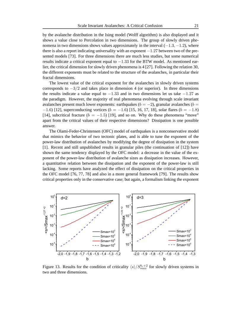
Figure 13. Results for the condition of criticality〈s〉/Sbc+2max for slowly driven systems in
two and three dimensions.
22 O. Ramos
of the power-law to the critical properties of the system is still missing. From the eqs. 27and 28 it is possible to get a condition of criticality for scale invariant avalanches:
〈s〉
Sbc+2max
∼ 1 (31)
with the considerations ofbc = −1.27 andbc = −1.33 for two and three dimensions re-spectively, in the case of slowly driven systems. The results of this condition of criticalityare displayed in figure 13, where the system separates exponentially from the critical situa-tion as the exponentb decreases. For a given exponent the decrease grows linearlywith themaximum avalanche sizeSmax.
In section 2.3.3. an energy balance limited the SOC in forbidding large values ofb (closeto −1) for dissipative slowly driven system. Now the results indicate that as the exponentdecreases, which in different systems is a consequence of the dissipations, the system losesits critical properties. The combination of both results restrict SOC to conservative andcritical models, like the original BTW one. This argument isin agreement with recentresults in avalanche prediction, which is the main subject of the next section.
5. Towards Prediction and Control
Several works have claimed the unpredictable character of phenomena evolving throughscale invariant avalanches (earthquakes, granular piles,solar flares, stock markets, etc) as aconsequence of their classification as critical systems [44, 80]. However, in the last section ithas been suggested that those systems are not critical, which is expressed in the small valueof the exponent of their power-laws compared to the criticalexponent at their respectivedimensions. If they are not critical, they are, in principle, predictable; a fact that has beenrecently proved in both experiments and simulations.
5.1. Predicting scale invariant avalanches
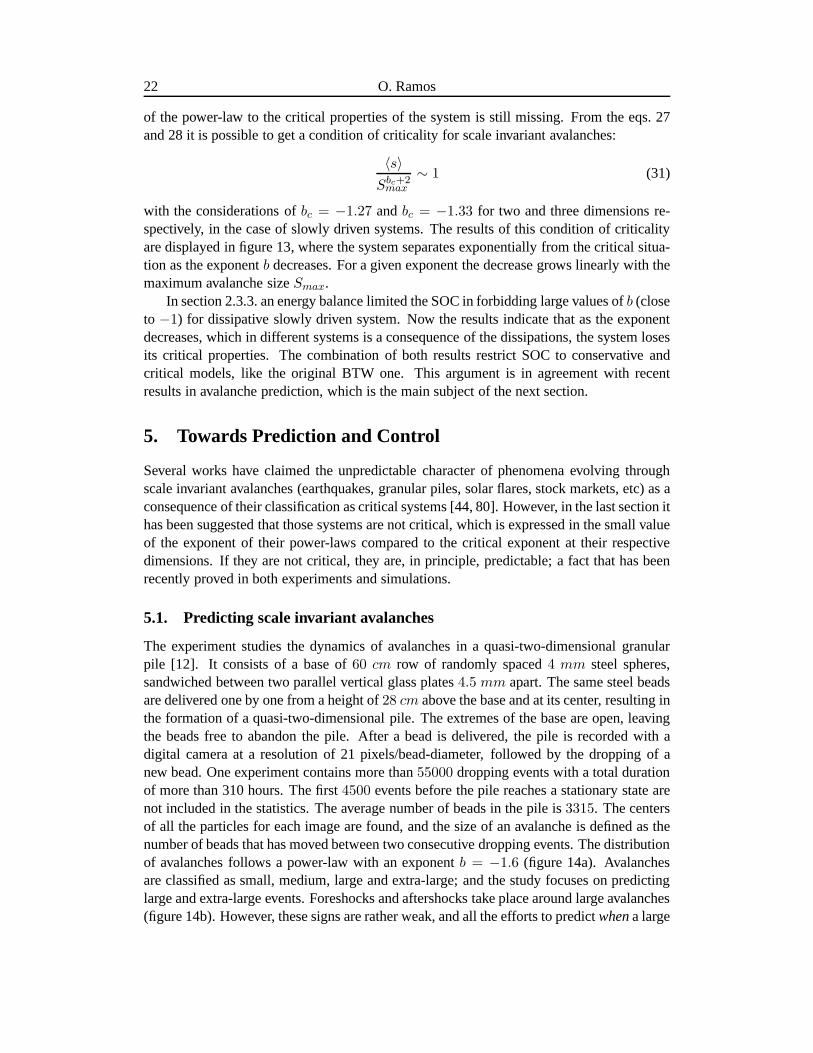
The experiment studies the dynamics of avalanches in a quasi-two-dimensional granularpile [12]. It consists of a base of60 cm row of randomly spaced4 mm steel spheres,sandwiched between two parallel vertical glass plates4.5 mm apart. The same steel beadsare delivered one by one from a height of28 cm above the base and at its center, resulting inthe formation of a quasi-two-dimensional pile. The extremes of the base are open, leavingthe beads free to abandon the pile. After a bead is delivered,the pile is recorded with adigital camera at a resolution of 21 pixels/bead-diameter,followed by the dropping of anew bead. One experiment contains more than55000 dropping events with a total durationof more than 310 hours. The first4500 events before the pile reaches a stationary state arenot included in the statistics. The average number of beads in the pile is3315. The centersof all the particles for each image are found, and the size of an avalanche is defined as thenumber of beads that has moved between two consecutive dropping events. The distributionof avalanches follows a power-law with an exponentb = −1.6 (figure 14a). Avalanchesare classified as small, medium, large and extra-large; and the study focuses on predictinglarge and extra-large events. Foreshocks and aftershocks take place around large avalanches(figure 14b). However, these signs are rather weak, and all the efforts to predictwhena large
Scale Invariant Avalanches: A Critical Confusion 23
-200 -100 0 100 200
15
20
25
220225230
100 101 102 103
100
101
102
103
104
Aftershocks
Ave
rage
ava
lanc
he s
ize
Time (dropping events)
Foreshocks
XL
4 %
b
b=-1,6 0,8 %
15,4 %
L
M
Num
ber o
f eve
nts
Avalanche size (number of beads)
S61,2 %
a
Figure 14. (a) Distribution of avalanche size for the granular experiment (circles). Thesepoints have been averaged with a logarithmic binning (diamonds) and they follow a power-law with an exponentb = −1.6. Avalanches have been classified as small (S), medium (M),large (L) and extra-large (XL). The percentage of occurrence of each type of avalanche isalso displayed. (b) The average of the avalanche size arounda large event (L) presents weaksigns of foreshocks and aftershocks.
avalanche is going to happen did not succeed: the analysis ofthe time series does not allowthe prediction of large events.
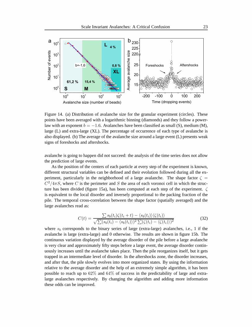
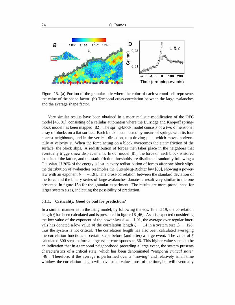
As the position of the centers of each particle at every step of the experiment is known,different structural variables can be defined and their evolution followed during all the ex-periment, particularly in the neighborhood of a large avalanche. The shape factorζ =C2/4πS, whereC is the perimeter andS the area of each voronoi cell in which the struc-ture has been divided (figure 15a), has been computed at each step of the experiment.ζis equivalent to the local disorder and inversely proportional to the packing fraction of thepile. The temporal cross-correlation between the shape factor (spatially averaged) and thelarge avalanches read as:
C(t) =
∑
sb(ti)ζ(ti + t)− 〈sb(ti)〉〈ζ(ti)〉√
∑
(sb(ti)− 〈sb(ti)〉)2∑
(ζ(ti)− 〈ζ(ti)〉)2(32)
wheresb corresponds to the binary series of large (extra-large) avalanches, i.e., 1 if theavalanche is large (extra-large) and 0 otherwise. The results are shown in figure 15b. Thecontinuous variation displayed by the average disorder of the pile before a large avalancheis very clear and approximately fifty steps before a large event, the average disorder contin-uously increases until the avalanche takes place. Then the pile reorganizes itself, but it getstrapped in an intermediate level of disorder. In the aftershocks zone, the disorder increases,and after that, the pile slowly evolves into more organized states. By using the informationrelative to the average disorder and the help of an extremelysimple algorithm, it has beenpossible to reach up to62% and64% of success in the predictability of large and extra-large avalanches respectively. By changing the algorithm and adding more informationthese odds can be improved.
24 O. Ramos
Figure 15. (a) Portion of the granular pile where the color ofeach voronoi cell representsthe value of the shape factor. (b) Temporal cross-correlation between the large avalanchesand the average shape factor.
Very similar results have been obtained in a more realistic modification of the OFCmodel [46, 81], consisting of a cellular automaton where theBurridge and Knopoff spring-block model has been mapped [82]. The spring-block model consists of a two dimensionalarray of blocks on a flat surface. Each block is connected by means of springs with its fournearest neighbours, and in the vertical direction, to a driving plate which moves horizon-tally at velocityv. When the force acting on a block overcomes the static friction of thesurface, the block slips. A redistribution of forces then takes place in the neighbors thateventually triggers new displacements. In our model [81], the force on each block is storedin a site of the lattice, and the static friction thresholds are distributed randomly following aGaussian. If20% of the energy is lost in every redistribution of forces afterone block slips,the distribution of avalanches resembles the Gutenberg-Richter law [83], showing a power-law with an exponentb = −1.91. The cross-correlation between the standard deviation ofthe force and the binary series of large avalanches donates aresult very similar to the onepresented in figure 15b for the granular experiment. The results are more pronounced forlarger system sizes, indicating the possibility of prediction.
5.1.1. Criticality. Good or bad for prediction?
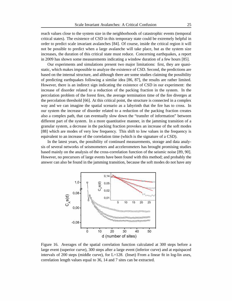
In a similar manner as in the Ising model, by following the eqs. 18 and 19, the correlationlengthξ has been calculated and is presented in figure 16 [46]. As it isexpected consideringthe low value of the exponent of the power-lawb = −1.91, the average over regular inter-vals has donated a low value of the correlation lengthξ = 14 in a system sizeL = 128;thus the system is not critical. The correlation length has also been calculated averagingthe correlation functions at certain steps before (and after) a large event. The value ofξcalculated 300 steps before a large event corresponds to 36.This higher value seems to bean indication that in a temporal neighborhood preceding a large event, the system presentscharacteristics of a critical state, which has been denominated “temporal critical state”[46]. Therefore, if the average is performed over a “moving”and relatively small timewindow, the correlation length will have small values most of the time, but will eventually
Scale Invariant Avalanches: A Critical Confusion 25
reach values close to the system size in the neighborhoods ofcatastrophic events (temporalcritical states). The existence of CSD in this temporary state could be extremely helpful inorder to predict scale invariant avalanches [84]. Of course, inside the critical region it willnot be possible to predict when a large avalanche will take place, but as the system sizeincreases, the duration of this critical state must reduce.Concerning earthquakes, a reportin 2009 has shown some measurements indicating a window duration of a few hours [85].
Our experiments and simulations present two major limitations: first, they are quasi-static, which makes impossible to analyze the existence of CSD. Second, the predictions arebased on the internal structure, and although there are somestudies claiming the possibilityof predicting earthquakes following a similar idea [86, 87], the results are rather limited.However, there is an indirect sign indicating the existenceof CSD in our experiment: theincrease of disorder related to a reduction of the packing fraction in the system. In thepercolation problem of the forest fires, the average termination time of the fire diverges atthe percolation threshold [66]. At this critical point, thestructure is connected in a complexway and we can imagine the spatial scenario as a labyrinth that the fire has to cross. Inour system the increase of disorder related to a reduction ofthe packing fraction createsalso a complex path, that can eventually slow down the “transfer of information” betweendifferent part of the system. In a more quantitative manner,in the jamming transition of agranular system, a decrease in the packing fraction provokes an increase of the soft modes[88] which are modes of very low frequency. This shift to low values in the frequency isequivalent to an increase of the correlation time (which is the signature of a CSD).
In the latest years, the possibility of continued measurements, storage and data analy-sis of several networks of seismometers and accelerometershas brought promising studiesbased mainly on the analysis of the cross-correlation function of the seismic noise [89, 90].However, no precursors of large events have been found with this method; and probably theanswer can also be found in the jamming transition, because the soft modes do not have any
0 10 20 30 40 50
-0,08
0,00
0,08
1,0
5 10 15 20 250,01
0,02
0,05
0,14
d (number of sites)
CAs(
d)
CAs(
d)
Figure 16. Averages of the spatial correlation function calculated at 300 steps before alarge event (superior curve), 300 steps after a large event (inferior curve) and at equispacedintervals of 200 steps (middle curve), for L=128. (Inset) From a linear fit in log-lin axes,correlation length values equal to 36, 14 and 7 sites can be extracted.
26 O. Ramos
influence on the elastic properties of the medium.
5.2. The origin of Scale invariant avalanches
The origin of the temporal scale invariance in nature has been a question of debate for morethan two decades [24, 91, 92]. Being able to group many different phenomena (earthquakes,granular avalanches, solar flares, stock markets, etc) intothe same kind of dynamics, wherecatastrophic events and small events are explained by the same principles, was an extraor-dinary achievement of the SOC. However, the axiomatic manner in which the base of thetheory was introduced, related to the existence of a critical state as an attractor of the dy-namics, set SOC as a theory to be proved more than as a theory todevelop. This hasprovoked that several relevant questions concerning scaleinvariant avalanches have neverbeen formulated in a direct manner; the influence of the dissipation and the influence of thedisorder in the “self-organization” are examples of these questions.
Although there is not quantitative results about the two proposed questions, two decadesof work on the subject have left some hints about them: the effect of the dissipation onmodifying the exponent of the power-law has already been discussed in section 4.2.; andnow let us analyze the influence of the disorder in the “self-organization” towards scaleinvariant avalanches. Two cases are going to be discussed: agranular pile and an earthquakemodel. In these situations (as well as all the other SOC systems) an energy gap controlsthe limits of the dynamics, i.e., the largest amount of dissipated energy. In the granularpile two angles define the energy gap: the subcritical angle and the supercritical angle [93].In ideal conditions (little disorder and large friction) a trivial periodic behavior rules thedynamics [4, 94, 95, 96], charging and discharging the energy gap. In the earthquake model[1, 81] there is some elastic energy stored in every site of a lattice, which is limited by localthresholds related to a static friction coefficient. The largest possible avalanche happenswhen all the sites have reached their thresholds and, with the trivial condition of a flatdistribution of thresholds, a trivial periodic behavior also rules the dynamics.
Disorder
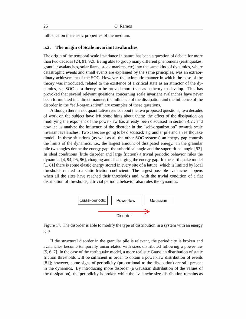
GaussianPower-lawQuasi-periodic
Figure 17. The disorder is able to modify the type of distribution in a system with an energygap.
If the structural disorder in the granular pile is relevant,the periodicity is broken andavalanches become temporally uncorrelated with sizes distributed following a power-law[5, 6, 7]. In the case of the earthquake model, a more realistic Gaussian distribution of staticfriction thresholds will be sufficient in order to obtain a power-law distribution of events[81]; however, some signs of periodicity (proportional to the dissipation) are still presentin the dynamics. By introducing more disorder (a Gaussian distribution of the values ofthe dissipation), the periodicity is broken while the avalanche size distribution remains as
Scale Invariant Avalanches: A Critical Confusion 27
a power-law. Nevertheless, increasing the values of the standard deviation of the Gaussiandistribution will lead to the removal of the power-law behavior [81]. These simulationswere focused on the SOC behavior; thus no more disorder was introduced after the ruptureof the scale invariance; though it is evident that if a disorder is artificially increased, aGaussian distribution behavior must be obtained. A simple example will be not respectingthe separation of scales (drive and dissipation) required for a scale invariant behavior, andto drive continually a granular pile. The result will be a continuous flow and a Gaussianbehavior will be obtained.
Predicting scale invariant avalanches in natural phenomena (particularly earthquakes),is one of the biggest challenges of today’s science. However, predicting catastrophic avalanchesit is not the final solution to this problem. The question to address is more practical: Is itpossible to control scale invariant avalanches? The simplest solution in order to break thescale invariance is theearly triggering, which is currently used in snow avalanches and innumerical models [97] to avoid large accumulations leadingto catastrophic events. Un-derstanding the role of dissipation, disorder, and other factors linked to the organizationof a system into a dynamics of scale invariant avalanches, can be essential in the futuredevelopment of tools leading to the control of catastrophicavalanches.
6. Conclusion
The essential role of the exponent value of the power-law distribution of avalanche sizeshas been discussed. The exponent value controls the proportion between small and largeevents in the dynamics. For an exponentb = −1, for example, the probability of largeand small events is the same (considering a logarithmic resolution). As the exponent valuedecreases (increases in absolute value), smaller events have more weight in the dynamics.This is also presented in the value of〈s〉, related to the energy balance in the system, andforbidding exponents close tob = −1 for slowly driven systems. The exponent value alsocontrols the critical properties of the system through thecondition of criticality〈s〉/Sbc+2
max
wherebc corresponds to the critical exponent for slowly driven systems, withbc ∼ −1.27andbc ∼ −1.33 in two and three dimensions respectively.
The causes, consequences, as well as some history of the logarithmic scale have alsobeen presented. The logarithmic scale is the only scale thatrespects the scale invarianceduring the measurement. The fact that an integration is performed during the measurementchanges the value of the exponent in+1 unit, which has provoked some confusion in theinterpretation of the distribution of earthquakes. However, it has been shown that a power-law with an exponentb = −2, and the consideration of one earthquake occurring every0.21 seconds, fits quite well the real data.
Simulation on a well established critical system (the Isingmodel) has revealed thatpower-law distributed avalanches are not a necessary condition in order to classify a sys-tem ascritical, but different kinds of distributions can rule the avalanche behavior of anequilibrium system at the critical point: A “Metropolis” algorithm displayed avalanchesdistributed following a Gaussian, while the “Wolff” algorithm presented a scale invariantdynamics with a critical exponentb = −1.1. Different experiments have shown differentkind of dynamics.
28 O. Ramos
Real scale invariant phenomena (earthquakes, granular piles, solar flares, etc) normallypresent exponent values far from the critical ones, and simulations and table experimentssuggest that dissipation is the cause of these low values. Asthe exponent moves apart fromthe the critical value, thecondition of criticality indicates that the system is loosing thecritical properties, thus it becomes, in principle, predictable. Prediction of scale invariantavalanches has been achieved both in a quasi-two-dimensional granular pile (b = −1.6)and in an earthquake model (b = −1.91). The correlation lengthξ has been calculated inthe earthquake model showing a low value when the correlation function is averaged overthe whole dynamics (or non correlated events). However, ifξ is calculated averaging thecorrelation function over a small time window, it presents small values most of the time, buteventually it reaches values proportional to the system size preceding catastrophic events,a situation denominated“temporal critical state”. The analysis of this temporal state caneventually be used to forecast real catastrophic avalanches.
The influence of dissipation and disorder in the “self-organization” of scale invariantdynamics have been discussed in a qualitative manner. However, quantitative studies arestill missing. These studies can eventually have an impact in the prediction and control ofreal catastrophic avalanches.
7. Acknowledgments
I am pleased to thank N. Arnesen and O. Duran for proofreadingthe manuscript; E. Alt-shuler, S. Ciliberto, O. Duran, P. Holdsworth, K. J. Maløy,T. Roscilde, S. Santucci and L.Vanel for useful discussions; J.-F. Pinton for sharing someexperimental data; R. Planet andS. Santucci for providing the figure 10; and C. Creton and A. Lindner for a lot of supportduring the writing of this chapter. I am also pleased to thankHenrik Jeldtoft Jensen, whoreviewed the manuscript and made very useful comments. Thiswork has been financed bythe European project MODIFY.
References
[1] Olami, Z.; Feder, H. J. S.; Christensen, K.Phys. Rev. Lett.1992, 68, 1244.
[2] Bak, P.; Tang C.J. Geophys. Res.1989, 94 (15) 635.
[3] Jagla, E. A.Phys. Rev. E2010, 81, 046117.
[4] Held, A. et al.Phys. Rev. Lett.1990, 65, 1120.
[5] Frette, V. et al.Nature1996, 379, 49.
[6] Altshuler, E.; Ramos, O.; Martınez, C.; Flores, L. E.; Noda, C.Phys. Rev. Lett.2001,86, 5490.
[7] Aegerter, C. M.; Gunther, R.; Wijngaarden, R. J.Phys. Rev. E2003, 67, 051306.
[8] Costello, R. M. et al.Phys. Rev. E2003, 67, 041304.
Scale Invariant Avalanches: A Critical Confusion 29
[9] Nerone, N.; Aguirre, M. A.; Calvo, A.; Bideau, D.; Ippolito, I. Phys. Rev. E2003, 67,011302.
[10] Aegerter, C. M.; Lorincz, K. A.; Welling, M. S.; Wijngaarden, R. J.Phys. Rev. Lett.2004, 92, 058702.
[11] Lorincz, K. A.; Wijngaarden, R. J.Phys. Rev. E2007, 76, 040301(R).
[12] Ramos, O.; Altshuler, E.; Maløy, K. J.Phys. Rev. Lett.2009, 102, 078701.
[13] Birkeland, K. W.; Landry, C. C.Geophys. Res. Lett.2002, 29 (11), 1554.
[14] Hamon, D.; Nicodemi, M.; Jensen, H. J.Astron. Astrophys.2002, 387, 326334.
[15] Bassler, K.; Paczuski, M.Phys. Rev. Lett.1998, 81, 37613764.
[16] Altshuler, E.; Johansen, T. H.Rev. Mod. Phys.2004, 76, 471487.
[17] Altshuler, E. et al.Phys. Rev. B2004, 70, 140505(R).
[18] Altshuler, E. et al.Physica C2004, 501, 408-410.
[19] Santucci, S.; Vanel, L.; Ciliberto, S.Phys. Rev. Lett.2004, 93, 095505
[20] Sneppen, K.; Bak, P.; Flyvbjerg, H.; Jensen, M. H.PNAS1995, 92, 5209.
[21] Lee, Y.; Nunes Amaral, L. A.; Canning, D.; Meyer, M.; Stanley, H. E.Phys. Rev. Lett.1998, 81, 3275.
[22] Bak, P.; Tang C.; Wiesenfeld K.Phys. Rev. Lett.1987, 59, 381-384.
[23] Jensen, H. J.Self-Organized Criticality, Emergent Complex Behavior inPhysical andBiological Systems;Cambridge Univ. Press: Cambridge, 1998.
[24] Bak, P.How Nature works-The Science of Self-organized Criticality; Oxford Univ.Press: Oxford, 1997.
[25] Alstrøm, P.Phys. Rev. A1988, 38, 4905-4906.
[26] Pietronero, L.; Vespignani, A.; Zapperi, S.Phys. Rev. Lett.1994, 72, 1690.
[27] Vespignani, A.; Zapperi, S.Phys. Rev. Lett.1997, 78, 4793-4796.
[28] Mandelbrot, B. B.Les Objets fractals, forme, hasard et dimension;Flammarion:Paris, 1975.
[29] Mandelbrot, B. B.The Fractal Geometry of Nature;W. H. Freeman & Co: San Fran-cisco, CA, 1982.
[30] Koch, H. V. In Classics on Fractals;Edgar, G. A.; Ed.; Addison-Wesley, ReadingMA, 1993.
[31] Gutenberg, B.; Richter, C. F.Ann. Geophys.1956, 9, 1-15.
30 O. Ramos
[32] Peek, J. B. H.; Bergmans, J. W. M.; Haaren, J. A. M. M.; Toolenaar, F.; Stan, S.G. Origins and Successors of the Compact Disc;Eindhoven, 2009; Philips ResearchBook Series, Vol. 11.
[33] Russ, J. C.The image processing handbook;CRS Press: Boca Raton, FL, 2002; pp23.
[34] Pogson, N. R.Mon. Not. R. Astron. Soc.1856, 17, 12-15.
[35] Ptolemy. First printed inAlmagestum Cl. Ptolemei;Venice, 1515.
[36] Toomer, G. T. InDictionary of Scientific Biography;Gillespie, C. C.; Ed.; CharlesScribner, New York, 1978; Vol. 15, pp 207-224.
[37] Fechner, G. T.Elemente der Psychophysik;Breitkopf und Hartel Leipzig, 1860.
[38] Stevens, S. S.Science1961, 133, 8086.
[39] Richter, C. F.Bull. Seismol. Soc. Am.1935, 25, 1-32.
[40] Los Angeles Times. (October 01, 1985) Charles F. Richter Dies; Earthquake ScalePioneer.
[41] Richter, C. F.Elementary Seismology;W. H. Freeman & Co: San Francisco, CA,1958; pp 135-149; 650-653.
[42] Sethna, J. P.Statistical Mechanics: Entropy, Order Parameters, and Complexity;Clarendon press: Oxford, 2009; pp 265.
[43] Bak, P.; Christensen, K.; Danon, L.; Scanlon, T.Phys. Rev. Lett.2002, 88, 178501.
[44] Main, I. Nature Debate 25 February to 8 April (1999).http://www.nature.com/nature/debates/earthquake/equake frameset.html
[45] U.S. Geological Survey (2010). Earthquake Facts and Statistics.http://earthquake.usgs.gov/earthquakes/eqarchives/year/eqstats.php
[46] Ramos, O.Tectonophysics2010, 485 321-326.
[47] Pruesner, G.; Peters, O.Phys. Rev. E2006, 73, 025106(R).
[48] Stanley, H. E.Introduction to Phase Transitions and Critical Phenomena;OxfordUniv. Press: New York, 1987.
[49] Clusel, M.; Fortin, J.-Y.; Holdsworth, P. C. W.Phys. Rev. E2004, 70, 046112.
[50] Newman, M. E. J.; Barkema, G. T.Monte Carlo Methods in Statistical Physics;Ox-ford Univ. Press: New York, 1999.
[51] Onsager, L.Phys. Rev.1944, 65, 117.
[52] Stauffer, D.Int. J. Mod. Phys. C1998, 9, 562.
Scale Invariant Avalanches: A Critical Confusion 31
[53] Bramwell, S. T. et al.Phys. Rev. Lett.2000, 84, 3744.
[54] Bramwell, S. T.; Holdsworth, P. C. W.; Pinton, J.-F.Nature1998, 396, 552.
[55] Metropolis, N. et al.J. Chem. Phys.1953, 21, 1087.
[56] Wolff, U. Phys. Rev. Lett.1989, 62, 361.
[57] Joubaud, S.; Petrosyan, A.; Ciliberto, S.; Garnier, N.B. Phys. Rev. Lett.2008, 100,180601.
[58] Planet, R.; Santucci, S.; Ortın, J.Phys. Rev. Lett.2009, 102, 094502.
[59] Dunlavy, M. J.; Venus, D.Phys. Rev. B2005, 71, 144406.
[60] Ciliberto, S. Private communication.
[61] Sethna, J. P.; Dahmen, K. A.; Myers, C. R. InScale Invariance and Beyond;Dubrulle,B.; Graner, F.; Sornette, D.; Ed.; Springer, Berlin, 1997, Les Houches Workshop,March 10-14, pp 87.
[62] Sethna, J. P.; Dahmen, K. A.; Myers, C. R.Nature2001, 410, 242.
[63] Zapperi, S.; Cizeau, P.; Durin, G.; Stanley, H. E.Phys. Rev. B1998, 58, 63536366.
[64] Barkhausen, H.Z Phys.1919, 20, 401.
[65] Labbe, R.; Pinton, J.-F.; Fauve, S.J. Phys. II France1996, 6, 1099-1110.
[66] Stauffer, D; Aharony, A.Introduction to Percolation Theory;Taylor & Francis: Lon-don, 1994.
[67] Harris, T. E.The theory of branching processes;Springer-Verlag: Berlin, 1963.
[68] Obukhov, S. P. InRandom Fluctuations and Pattern Growth;Stanley, H. E.; Os-trowsky, N.; Ed.; Kluwer, Dordrecht, 1988.
[69] Dıaz-Guilera, A.Europhys. Lett.1994, 26, 177.
[70] Le Doussal, P.; Wiese, K. J.Phys. Rev. E2009, 79, 051106.
[71] Lauritsen, K. B.; Zapperi, S.; Stanley, H. E.Phys. Rev. E1996, 54, 2483-2488.
[72] Manna, S. S.J. Stat. Phys.1990, 59, 509.
[73] Chessa, A.; Stanley, H. E.; Vespignani, A.; Zapperi, S.Phys. Rev. E1999, 59, R12-R15.
[74] Lubeck, S.; Usadel, K. D.Phys. Rev. E1997, 56, 5138-5143.
[75] Tang. C.; Bak, P.Phys. Rev. Lett.1998, 60, 2347-2350.
[76] Carvalho, J. X. de; Prado, C. P. C.Phys. Rev. Lett.2000, 84, 4006.
32 O. Ramos
[77] Miller, G.; Boulter, C. J.Phys. Rev. E2002, 66, 016123.
[78] Xia, J.; Gould, H.; Klein, W.; Rundle, J. B.Phys. Rev. E2008, 77, 031132.
[79] Bonachela, J. A.; Munoz, M. A.J. Stat. Mech.2009, P09009, 1742-5468.
[80] R. J. Geller, R. J.; Jackson, D. D.; Kagan, Y. Y.; Mulargia, F.Science1997, 275, 1616.
[81] Ramos, O.; Altshuler, E.; Maløy, K. J.Phys. Rev. Lett.2006, 96, 098501.
[82] Burridge, R.; Knopoff, L.J. Geophys. Res. Bull. Seismol. Soc. Am.1967, 57, 341.
[83] Christensen, K.; Olami, Z.J. Geophys. Res.1992, 97, B6, 8729-8735.
[84] Scheffer, M. et al.Nature2009, 461, 53-59.
[85] Manshour, P. et al.Phys. Rev. Lett.2009, 102, 014101.
[86] Crampin, S.; Gao, Y.; Peacock, S.Geology2008, 36, 427-430.
[87] Crampin, S.; Gao, YGeophysical Journal International2010, 180, 1124.
[88] Wyart, M.; Silbert. L. E.; Nagel, S. R.; Witten, T. A.Phys. Rev. E2005, 72, 051306.
[89] Brenguier, F. et al.Science2008, 321, 1478.
[90] Brenguier, F. et al.Nature Geoscience2008, 1, 126.
[91] Vespignani, A.; Zapperi, S.Phys. Rev. E1998, 57, 6345.
[92] Reed, W. J.; Hughes, B. D.Phys. Rev. E2002, 66, 067103.
[93] Daerr, A.; Douady, S.Nature1999, 399, 241.
[94] Jaeger, H. M.; Liu, C.; Nagel.; S. R.Phys. Rev. Lett.1989, 62, 4043.
[95] Rosendahl, J.; Vekic, M.; Kelley J.Phys. Rev. E1993, 47, 14011404.
[96] Rosendahl, J.; Vekic, M.; Rutledge J. E.Phys. Rev. Lett.1994, 73, 537540.
[97] Cajueiro, D. O.; Andrade, R. F. S.Phys. Rev. E2010, 81, 015102(R).
Related Documents

![arXiv:1502.04383v3 [cs.CV] 16 Jul 2016 · 2016. 7. 19. · 1 arXiv:1502.04383v3 [cs.CV] 16 Jul 2016. Pose r Invariant Face Recognition (PIFR) Algorithms Face Matching profile half](https://static.cupdf.com/doc/110x72/5fdd44d75ec6946e6157dac5/arxiv150204383v3-cscv-16-jul-2016-2016-7-19-1-arxiv150204383v3-cscv.jpg)


![arXiv:1504.04338v1 [math.CV] 16 Apr 2015 · arXiv:1504.04338v1 [math.CV] 16 Apr 2015 BOUNDARY MULTIPLIERS OF A FAMILY OF MOBIUS INVARIANT FUNCTION¨ SPACES GUANLONG BAO AND JORDI](https://static.cupdf.com/doc/110x72/5f7b4fff8c891c00121fec72/arxiv150404338v1-mathcv-16-apr-2015-arxiv150404338v1-mathcv-16-apr-2015.jpg)


![Computing a categorical GromovWitten invariant arXiv:1706 ...andreic/publications/CatGWEll.pdf · arXiv:1706.09912v2 [math.AG] 11 Jul 2017 Computing a categorical GromovWitten invariant](https://static.cupdf.com/doc/110x72/5ff09e03c26eae3310726ec5/computing-a-categorical-gromovwitten-invariant-arxiv1706-andreicpublications.jpg)