Scalable Load Balancing Techniques for Parallel Computers

Scalable Load Balancing Techniques for Parallel Computers�Vipin Kumar and Ananth Y. GramaDepartment of Computer Science,University of MinnesotaMinneapolis, MN 55455andVempaty Nageshwara RaoDepartment of Computer ScienceUniversity of Central FloridaOrlando, Florida 32816AbstractIn this paper we analyze the scalability of a number of load balancing algorithms which canbe applied to problems that have the following characteristics : the work done by a processorcan be partitioned into independent work pieces; the work pieces are of highly variable sizes;and it is not possible (or very di�cult) to estimate the size of total work at a given processor.Such problems require a load balancing scheme that distributes the work dynamically amongdi�erent processors.Our goal here is to determine the most scalable load balancing schemes for di�erent archi-tectures such as hypercube, mesh and network of workstations. For each of these architectures,we establish lower bounds on the scalability of any possible load balancing scheme. We presentthe scalability analysis of a number of load balancing schemes that have not been analyzedbefore. This gives us valuable insights into their relative performance for di�erent problem andarchitectural characteristics. For each of these architectures, we are able to determine nearoptimal load balancing schemes. Results obtained from implementation of these schemes in thecontext of the Tautology Veri�cation problem on the Ncube/2TM 1 multicomputer are used tovalidate our theoretical results for the hypercube architecture. These results also demonstratethe accuracy and viability of our framework for scalability analysis.1 IntroductionLoad balancing is perhaps the central aspect of parallel computing. Before a problem can be exe-cuted on a parallel computer, the work to be done has to be partitioned among di�erent processors.Due to uneven processor utilization, load imbalance can cause poor e�ciency. This paper investi-gates the problem of load balancing in multiprocessors for those parallel algorithms that have thefollowing characteristics.�This work was supported by Army Research O�ce grant # 28408-MA-SDI to the University of Minnesota andby the Army High Performance Computing Research Center at the University of Minnesota.1Ncube/2 is a trademark of the Ncube Corporation. 1

� The work available at any processor can be partitioned into independent work pieces as longas it is more than some non-decomposable unit.� The cost of splitting and transferring work to another processor is not excessive. (i:e: the costassociated with transferring a piece of work is much less than the computation cost associatedwith it.)� A reasonable work splitting mechanism is available; i.e., if work w at one processor is par-titioned in 2 parts w and (1 � )w, then 1 � � > > �, where � is an arbitrarily smallconstant.� It is not possible (or is very di�cult) to estimate the size of total work at a given processor.Although, in such parallel algorithms, it is easy to partition the work into arbitrarily manyparts, these parts can be of widely di�ering sizes. Hence after an initial distribution of work amongP processors, some processors may run out of work much sooner than others; therefore a dynamicbalancing of load is needed to transfer work from processors that have work to processors that areidle. Since none of the processors (that have work) know how much work they have, load balancingschemes which require this knowledge (eg. [17, 19]) are not applicable. The performance of a loadbalancing scheme is dependent upon the degree of load balance achieved and the overheads due toload balancing.Work created in the execution of many tree search algorithms used in arti�cial intelligenceand operations research [22, 31] and many divide-and-conquer algorithms [16] satisfy all the re-quirements stated above. As an example, consider the problem of searching a state-space tree indepth-�rst fashion to �nd a solution. The state space tree can be easily split up into many partsand each part can be assigned to a di�erent processor. Although it is usually possible to come upwith a reasonable work splitting scheme [29], di�erent parts can be of radically di�erent sizes, andin general there is no way of estimating the size of a search tree.A number of dynamic load balancing strategies that are applicable to problems with these char-acteristics have been developed [3, 7, 8, 10, 28, 29, 30, 33, 35, 36, 40, 41]. Many of these schemeshave been experimentally tested on some physical parallel architectures. From these experimen-tal results, it is di�cult to ascertain relative merits of di�erent schemes. The reason is that theperformance of di�erent schemes may be impacted quite di�erently by changes in hardware char-acteristics (such as interconnection network, CPU speed, speed of communication channels etc.),number of processors, and the size of the problem instance being solved [21]. Hence any conclu-sions drawn on a set of experimental results are invalidated by changes in any one of the aboveparameters. Scalability analysis of a parallel algorithm and architecture combination is very usefulin extrapolating these conclusions [14, 15, 21, 23]. It may be used to select the best architecture -algorithm combination for a problem under di�erent constraints on the growth of the problem sizeand the number of processors. It may be used to predict the performance of a parallel algorithmand a parallel architecture for a large number of processors from the known performance on fewerprocessors. Scalability analysis can also predict the impact of changing hardware technology on theperformance, and thus helps in designing better parallel architectures for solving various problems.Kumar and Rao have developed a scalability metric, called isoe�ciency , which relates theproblem size to the number of processors necessary for an increase in speedup in proportion to the2

number of processors used [23]. An important feature of isoe�ciency analysis is that it succinctlycaptures the e�ects of characteristics of the parallel algorithm as well as the parallel architectureon which it is implemented, in a single expression. The isoe�ciency metric has been found tobe quite useful in characterizing scalability of a number of algorithms [13, 25, 34, 37, 42, 43]. Inparticular, Kumar and Rao used isoe�ciency analysis to characterize the scalability of some loadbalancing schemes on the shared-memory, ring and hypercube architectures[23] and validated itexperimentally in the context of the 15-puzzle problem.Our goal here is to determine the most scalable load balancing schemes for di�erent architecturessuch as hypercube, mesh and network of workstations. For each architecture, we establish lowerbounds on the scalability of any possible load balancing scheme. We present the scalability analysisof a number of load balancing schemes that have not been analyzed before. From this we gainvaluable insights about which schemes can be expected to perform better under what problem andarchitecture characteristics. For each of these architectures, we are able to determine near optimalload balancing schemes. In particular, some of the algorithms analyzed here for hypercubes aremore scalable than those presented in [23]. Results obtained from implementation of these schemesin the context of the Tautology Veri�cation problem on the Ncube/2TM multicomputer are usedto validate our theoretical results for the hypercube architecture. The paper also demonstrates theaccuracy and viability of our framework for scalability analysis.Section 2 introduces the various terms used in the analysis. Section 3 presents the isoe�ciencymetric used for evaluating scalability. Section 4 reviews receiver initiated load balancing schemes,which are analyzed in Section 5. Section 6 presents sender initiated schemes and discusses theirscalability. Section 7 addresses the e�ect of variable work transfer cost on overall scalability. Section8 presents experimental results. Section 9 contains summary of results and suggestions for futurework.Some parts of this paper have appeared in [11] and [24].2 De�nitions and AssumptionsIn this section, we introduce some assumptions and basic terminology necessary to understand theisoe�ciency analysis.1. Problem size W : the amount of essential computation (i:e:, the amount of computation doneby the best sequential algorithm) that needs to be performed to solve a problem instance.2. Number of processors P : number of identical processors in the ensemble being used to solvethe given problem instance.3. Unit Computation time Ucalc: the time taken for one unit of work. In parallel depth-�rstsearch, the unit of work is a single node expansion.4. Computation time Tcalc: is the sum of the time spent by all processors in useful computation.(Useful computation is that computation that would also have been performed by the bestsequential algorithm.) Clearly, since in solving a problem instance, we need to do W units ofwork, and each unit of work takes Ucalc time,3

Tcalc = Ucalc �W5. Running time TP : the execution time on a P processor ensemble.6. Overhead To: the sum of the time spent by all processors in communicating with otherprocessors, waiting for messages, time in starvation, etc. For a single processor, To = 0.Clearly, Tcalc + To = P � TP7. Speedup S: the ratio TcalcTP .It is the e�ective gain in computation speed achieved by using P processors in parallel on agiven instance of a problem.8. E�ciency E: the speedup divided by P . E denotes the e�ective utilization of computingresources. E = SP = TcalcTP � P= TcalcTcalc + To = 11 + ToTcalc9. Unit Communication time Ucomm: the mean time taken for getting some work from anotherprocessor. Ucomm depends upon the size of the message transferred, the distance betweenthe donor and the requesting processor, and the communication speed of the underlyinghardware. For simplicity, in the analysis of Sections 5 and 6, we assume that the messagesize is �xed. Later, in Section 7, we demonstrate the e�ect of variable message sizes on theoverall performance of the schemes.3 Isoe�ciency function : A measure of scalabilityIf a parallel algorithm is used to solve a problem instance of a �xed size, then the e�ciencydecreases as number of processors P increases. The reason is that the total overhead increaseswith P . For many parallel algorithms, for a �xed P , if the problem size W is increased, then thee�ciency becomes higher (and approaches 1), because the total overhead grows slower than W .For these parallel algorithms, the e�ciency can be maintained at a desired value (between 0 and1) with increasing number of processors, provided the problem size is also increased. We call suchalgorithms scalable parallel algorithms.Note that for a given parallel algorithm, for di�erent parallel architectures, the problem sizemay have to increase at di�erent rates w.r.t. P in order to maintain a �xed e�ciency. The rateat which W is required to grow w.r.t. P to keep the e�ciency �xed is essentially what determinesthe degree of scalability of the parallel algorithm for a speci�c architecture. For example, if Wis required to grow exponentially w.r.t. P , then the algorithm-architecture combination is poorly4

scalable. The reason for this is that in this case it would be di�cult to obtain good speedups on thearchitecture for a large number of processors, unless the problem size being solved is enormouslylarge. On the other hand, ifW needs to grow only linearly w.r.t. P , then the algorithm-architecturecombination is highly scalable and can easily deliver linearly increasing speedups with increasingnumber of processors for reasonable increments in problem sizes. If W needs to grow as f(P ) tomaintain an e�ciency E, then f(P ) is de�ned to be the isoe�ciency function for e�ciency Eand the plot of f(P ) w.r.t. P is de�ned to be the isoe�ciency curve for e�ciency E.As shown in [21], an important property of a linear isoe�ciency function, is that the problem sizecan be increased linearly with the number of processors while maintaining a �xed execution time ifand only if the isoe�ciency function is �(P ). Also, parallel systems with near linear isoe�cienciesenable us to solve increasingly di�cult problem instances in only moderately greater time. This isimportant in many domains (e:g: real time systems) in which we have only �nite time in which tosolve problems.A lower bound on any isoe�ciency function is that asymptotically, it should be at least linear.This follows from the fact that all problems have a sequential (i:e: non decomposable) component.Hence any algorithm which shows a linear isoe�ciency on some architecture is optimally scalableon that architecture. Algorithms with isoe�ciencies of O(P logc P ), for small constant c, are alsoreasonably optimal for practical purposes. For a more rigorous discussion on the isoe�ciency metricand scalability analysis, the reader is referred to [23, 21].3.1 Lower bounds on isoe�ciency functions for load balancing algorithms fordi�erent architecturesFor some algorithm - architecture combinations, it is possible to obtain a tighter lower boundthan O(P ) on the isoe�ciency. Consider a problem whose run time on a parallel architecture(comprising of P processors ) is given by TP . By de�nition, speedup for this problem is given byTcalcTP and e�ciency by TcalcP�TP . Thus for e�ciency to be a constant, TcalcP�TP must be constant andthus Tcalc should grow as �(P � TP ). Since Tcalc = W � Ucalc, W should also grow as �(P � TP ).Thus, if TP has a lower bound of (G(P )), we have a lower bound of (P �G(P )) on the on theisoe�ciency function.For the hypercube architecture, it takes at least (logP ) time for the work to propagate toall the processors (since the farthest processors are logP hops away). Thus the execution time forany load balancing algorithm running on a hypercube is lower bounded by (logP ). Hence theisoe�ciency function has a lower bound of (P log P ). On a mesh, it would take (pP ) time forthe work to propagate to all processors and consequently the lower bound on isoe�ciency is givenby (P 1:5). For the network of workstations, since for all processors to get work, there have to beat least P messages, and these have to be sent sequentially over the network, the execution time islower bounded by (P ) and the lower bound on isoe�ciency is given by (P 2).4 Receiver Initiated Load Balancing AlgorithmsIn this section, we brie y review receiver initiated load balancing algorithms that are analyzedin section 5. Many of these schemes have been presented in the context of speci�c architectures[28, 8, 29, 30, 40]. These schemes are characterized by the fact that the work splitting is performed5

'& $%'& $%'& $%'& $%

@@@@@@@@@@@I�����������6

?6

� -?

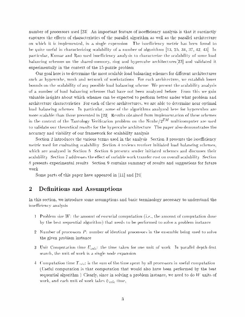
request it for work.Select a processor and Processor idle.Processor active.Got a reject.Issued a request. Got work.work.Finished available

Service any pending messages.Do a �xed amount of work.Service any pending messages.

Figure 1: State diagram describing the generic parallel formulation.only when an idle processor (receiver) requests for work. In all these schemes, when a processorruns out of work, it generates a request for work. The selection of the target of this work requestis what di�erentiates all these di�erent load balancing schemes. The selection of the target for awork request should be such as to minimize the total number of work requests and transfers as wellas load imbalance among processors.The basic load balancing algorithm is shown in the state diagram in Figure 4. At any giveninstant of time, some of the processors are busy (i:e: they have work) and the others are idle (i:e:they are trying to get work). An idle processor selects another processor as a target and sends it awork request. If the idle processor receives some work from the target processor, it becomes busy. Ifit receives a reject message (implying that there was no work available at the requested processor),it selects another target and sends it a work request. This is repeated until the processor gets work,or all the processors become idle. While in the idle state, if a processor receives a work request, itreturns a reject message.In the busy state, the processor does a �xed amount of work and checks for any pending6

work� request messages. If a work� request message was received then the work available at theprocessor is partitioned into two parts and one of the parts is given to the requesting processor. Iftoo little work is available, then a reject message is sent. When a processor exhausts its own work,it goes into the idle state.A termination detection algorithm runs in the background. This signals termination whenevera solution is found or all processors run out of work.4.1 Asynchronous Round Robin (ARR)In this scheme, each processor maintains an independent variable target. Whenever a processorruns out of work, it reads the value of this target and sends a work request to that particularprocessor. The value of the target is incremented (modulo P ) each time its value is read and awork request sent out. Initially, for each processor, the value of target is set to ((p+ 1)moduloP )where p is its processor identi�cation number. Note that work requests can be generated by eachprocessor independent of the other processors; hence the scheme is simple, and has no bottlenecks.However it is possible that work requests made by di�erent processors around the same time maybe sent to the same processor. This is not desirable since ideally work requests should be spreaduniformly over all processors that have work.4.2 Nearest Neighbor (NN)In this scheme a processor, on running out of work, sends a work request to its immediate neighborsin a round robin fashion. For example, on a hypercube, a processor will send requests only to itslogP neighbors. For networks in which distance between all pairs of processors is the same, thisscheme is identical to the Asynchronous Round Robin scheme. This scheme ensures locality ofcommunication for both work requests and actual work transfers. A potential drawback of thescheme is that localized concentration of work takes a longer time to get distributed to other faraway processors.4.3 Global Round Robin (GRR)Let a global variable called TARGET be stored in processor 0. Whenever a processor needs work,it requests and gets the value of TARGET; and processor 0 increments the value of this variableby 1 (modulo P ) before responding to another request. The processor needing work now sendsa request to the processor whose number is given by the value read from TARGET (i.e., the onesupplied by processor 0). This ensures that successive work requests originating in the system aredistributed evenly over all processors. A potential drawback of this scheme is that there will becontention for accessing the value of TARGET.4.4 GRR with Message combining. (GRR-M)This scheme is a modi�ed version of GRR that avoids contention over accessing TARGET. In thisscheme, all the requests to read the value of TARGET at processor 0 are combined at intermediateprocessors. Thus the total number of requests that have to be handled by processor 0 is greatlyreduced. This technique of performing atomic increment operations on a shared variable, TARGET,7

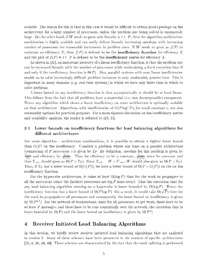
is essentially a software implementation of the fetch-and-add operation of [6]. To the best of ourknowledge, GRR-M has not been used for load balancing by any other researcher.We illustrate this scheme by describing its implementation for a hypercube architecture. Figure4.5 describes the operation of GRR-M for a hypercube multicomputer with P = 8. Here, we embeda spanning tree on the hypercube rooted at processor zero. This can be obtained by complimentingthe bits of processor identi�cation numbers in a particular sequence. We shall use the low to highsequence. Every processor is at a leaf of the spanning tree. When a processor wants to atomicallyread and increment TARGET, it sends a request up the spanning tree towards processor zero. Aninternal node of the spanning tree holds a request from one of its children for at most � time beforeit is sent to its parent. If a request comes from the other child within this time, it is combinedand sent up as a single request. If i represents the number of increments combined, the resultingincrement on TARGET is i and returned value for read is previous value of target. This is illustratedby the �gure where the total requested increment is 5 and the original value of TARGET, i:e: x,percolates down the tree. The individual messages combined are stored in a table until the requestis granted. When read value of TARGET is sent back to an internal node, two values are sent downto the left and right children if the value corresponds to a combined message. The two values canbe determined from the entries in the table corresponding to increments by the two sons.A similar implementation can be formulated for other architectures.4.5 Random Polling (RP).This is the simplest load balancing strategy where a processor requests a randomly selected pro-cessor for work each time it runs out of work. The probability of selection of any processor is thesame.4.6 Scheduler Based Load Balancing (SB)This scheme was proposed in [30] in the context of depth �rst search for test generation in VLSICAD applications. In this scheme, a processor is designated as a scheduler. The scheduler maintainsa queue (i:e: a FIFO list) called DONOR, of all possible processors which can donate work. InitiallyDONOR contains just one processor which has all the work. Whenever a processor goes idle, itsends a request to the scheduler. The scheduler then deletes this processor from the DONOR queue,and polls the processors in DONOR in a round robin fashion until it gets work from one of theprocessors. At this point, the recipient processor is placed at the tail of the queue and the workreceived by the scheduler is forwarded to the requesting processor.Like GRR, for this scheme too, successive work requests are sent to di�erent processors. How-ever, unlike GRR, a work request is never sent to any processor which is known to have no work.The performance of this scheme can be degraded signi�cantly by the fact that all messages ( includ-ing messages containing actual work ) are routed through the scheduler. This poses an additionalbottleneck for work transfer. Hence we modi�ed this scheme slightly so that the poll was still gen-erated by the scheduler but the work was transferred directly to the requesting processor insteadof being routed through the scheduler. If the polled processor happens to be idle, it returns a`reject' message to the scheduler indicating that it has no work to share. On receiving a `reject',the scheduler gets the next processor from the DONOR queue and generates another poll. It should8

l llllllll llll ll

h hh hh hhhPPPPPPPPPPi SSSSSSo AAAAK�� ����� �� ��7�� ���JJJJJJ] �� ���

�� �� �� ��1 ��� ��� ����� �����/ ����� AAAAUSSSSSSw������JJJJJJ������ � PPPPPPPPPPPq���������) AAAAAA������AAAAAA������LLLLLL������BBBBBB����� \\\\\\\������TTTTTTT PPPPPPPPPPP!!!!!!!!!!���� ������������

2 113 11 x+3 x+4x+3x+2 x+2x+2x+1x+1 11

211x x xAfter increment operation, TARGET = x+5.Initially TARGET = x.111110101100011010001000

100 110100010000000000

111101 100 110010011001 000

Figure 2: Illustration of message combining on an 8 processor hypercube.9

be clear to the reader that the modi�ed scheme has a strictly better performance compared to theoriginal scheme. This was also experimentally veri�ed by us.5 Scalability Analysis of Receiver Initiated Load Balancing Al-gorithmsTo analyze the scalability of a load balancing scheme, we need to compute To which is the extra workdone by the parallel formulation. Extra work done in any load balancing is due to communicationoverheads (i:e: time spent in requesting for work and sending work), idle time (when processor iswaiting for work), time spent in termination detection, contention over shared resources etc.For the receiver initiated schemes, the idle time is subsumed by the communication overheadsdue to work requests and transfers. This follows from the fact that as soon as a processor becomesidle, it selects a target for a work request and issues a request. The total time that it remains idleis the time taken for this message to reach the target and for the reply to arrive. At this point,either the processor becomes busy or it generates another work request. Thus the communicationoverhead gives the order of time that a processor is idle.The framework for setting upper bounds on overheads due to the communication overhead ispresented in Section 5.1. For isoe�ciency terms due to termination, we can show the followingresults. In the case of a network of workstations, we can implement a ring termination scheme,which can be implemented in �(P ) time. This contributes an isoe�ciency term of �(P 2). For ahypercube, we can embed a tree into the hypercube and termination tokens propagate up the tree.It can be shown that this contributes an isoe�ciency term of �(P log P ). In the case of a mesh,we can propagate termination tokens along rows �rst and then along columns. This techniquecontributes an isoe�ciency term of �(P 1:5). In each of these cases, the isoe�ciency term is of thesame asymptotic order as the lower bound derived in Section 3.1.5.1 A General Framework for Computing Upper Bounds on CommunicationDue to the dynamic nature of the load balancing algorithms being analyzed, it is very di�cultto come up with a precise expression for the total communication overheads. In this Section, wereview a framework of analysis that provides us with an upper bound on these overheads. Thistechnique was originally developed in the context of Parallel Depth First Search in [8, 23].We have seen that communication overheads are caused by work requests and work transfers.The total number of work transfers can only be less than the total number of work requests;hence the total number of work requests weighted with the total cost of one work request andcorresponding work transfer de�nes an upper bound on the total communication overhead. Forsimplicity, in the rest of this section, we assume constant message sizes; hence the cost associatedwith all the work requests generated de�nes an upper bound on the total communication overheads.In all the techniques being analyzed here, the total work is dynamically partitioned among theprocessors and processors work on disjoint parts independently, each executing the piece of workit is assigned. Initially an idle processor polls around for work and when it �nds a processor withwork of size Wi, the work Wi is split into disjoint pieces of size Wj and Wk . As stated in theintroduction, the partitioning strategy can be assumed to satisfy the following property -10

There is a constant � > 0 such that Wj > �Wi and Wk > �Wi .Recall that in a transfer, work (w) available in a processor is split into two parts (�w and(1��)w) and one part is taken away by the requesting processor. Hence after a transfer neither ofthe two processors (donor and requester) have more than (1��)w work ( note that � is always lessthan or equal to 0.5 ). The process of work transfer continues until work available in every processoris less than �. At any given time, there is some processor that has the maximum workload of allprocessors. Whenever a processor receives a request for work, its local workload becomes smaller(unless it is already less than �). If every processor is requested for work at least once, then we canbe sure that the maximum work at any of the processors has come down at least by a factor of(1� �). Let us assume that in every V(P) requests made for work, every processor in the systemis requested at least once. Clearly, V (P ) � P . In general, V(P) depends on the load balancingalgorithm. Initially processor 0 has W units of work, and all other processors have no work.After V (P ) requests maximum work available in any processor is less than (1� �)WAfter 2V (P ) requests maximum work available in any processor is less than (1� �)2W... After (log 11�� W� )V (P ) requests maximum work available in any processor is less than �.Hence total number of requests � V (P ) log 11�� WTo ' Ucomm � V (P ) log 11�� W (upper bound)Tcalc = UcalcWEfficiency = 11 + ToTcalc= 11 + Ucomm�V (P ) log 11�� WUcalc�WSolving this for isoe�ciency term due to communication gives us the relationW � UcommUcalc V (P ) logWW = O(V (P ) logW ) (1)The isoe�ciency de�ned by this term is the overall isoe�ciency of the parallel system if itasymptotically dominates all other terms (due to reasons other than the communication overhead).5.2 Computation of V(P) for various load balancing schemesClearly, it can be seen that V (P ) is �(P ) for GRR and GRR-M, and as shown in [8, 23] it isO(P 2) for Asynchronous Round Robin techniques. The worst case for Asynchronous Round Robintechniques is realized when all processors generate successive work requests at almost identicalinstances of time and the initial value of counters at all processors is almost identical. Considerthe following (worst case) scenario. Assume that processor P � 1 had all the work and the localcounters of all the other processors (0 to P � 2) were pointing to processor 0. In such a case,for processor P � 1 to receive a work request, one processor may have to request up to P � 111

processors and the remaining P � 2 processors in the meantime might have generated up to P � 2work requests (all processors except processor P � 1 and itself). Thus V (P ) in this case is given by(P � 1) + (P � 2)(P � 2), i.e. O(P 2). The readers must note that this is only an upper bound onthe value of V (P ), and the actual value of V (P ) is between P and P 2. For NN, V (P ) is unboundedfor architectures such as the hypercube. That is why isoe�ciency functions for NN are determinedin [23] using a di�erent technique.Random PollingIn the worst case, the value of V (P ) is unbounded for random polling. Here we present an averagecase analysis for computing the value of V (P ).Consider a system of P boxes. In each trial a box is picked up at random and marked o�. Weare interested in mean number of trials required to mark all the boxes. In our algorithm, each trialconsists of a processor requesting another processor selected at random for work.Let F (i; P ) represent a state of the system where i of the P boxes have been marked and i � Phave not been marked. Since the next box to be marked is picked at random, there is iP chancethat it will be a marked box and P�iP chance that it will be an unmarked box. Hence the systemremains in F (i; P ) with a probability of iP and transits to F (i + 1; P ) with a probability of P�iP .Let f(i; P ) denote the average number of trials needed to change from state F (i; P ) to F (P; P ).Obviously, V (P ) = f(0; P ).We have f(i; P ) = iP (1 + f(i; P )) + P � iP (1 + f(i+ 1; P ))P � iP f(i; P ) = 1 + P � iP f(i+ 1; P )f(i; P ) = PP � i + f(i+ 1; P )Hence, f(0; P ) = P ? �i=P�1i=0 1P � i= P ? �i=Pi=1 1i= P ? HPwhere HP denotes the harmonic mean of �rst P natural numbers. Since we have HP ' 1:69ln(P )(where ln(P ) denotes natural logarithm i:e: base e of P), we have V (P ) = �(P log P ). This valueof V(P) will be used to compute the isoe�ciency of RP on di�erent architectures.Scheduler Based Load BalancingFor this scheme, it can be seen that the length of the potential work donors can never exceed thetotal number of processors. At any given time, the processors that are not on the DONOR queueare known to have no work. Hence, the total maximum work at any processor in the system can bereduced by a factor of (1��) by issuing each of these processors a work request. Since a processor,on getting work is added to the end of the queue, and since the processors already in the DONORqueue are polled in a round robin fashion, it can be seen that no processor will be requested for12

work twice in a time interval when another busy processor was not requested even once. Since atany given point of time, this queue can not contain more than P processor (since duplication of aprocessor is not possible) P forms an upper bound on the number of requests that need to be madefor each processor with work to be requested at least once. Thus V (P ) is O(P ).5.3 Analysis of Receiver Initiated Load Balancing Algorithms for HypercubeHere we present analyses for all the schemes introduced in section 4 with the exception of NN.Scalability analysis for NN was presented in [23]. Some of the techniques analyzed here have betterscalability than the NN, and have near optimal isoe�ciency functions.In this section, we assume that work can be transferred through �xed size messages. The e�ectof relaxing this assumption is presented in Section 7.For a hypercube, the average distance between any randomly chosen pair of processors is�(logP ). On actual machines however, this asymptotic relation might not accurately describecommunication characteristics for the practical range of processors, and a more precise analysismay be required. Section 5.3.6 presents such an analysis and investigates the impact of actualcommunication parameters for the Ncube/2TM on the overall scalability of these schemes.In this section, we perform analysis with the asymptotic value of Ucomm = �(logP ).Equation 1 thus reduces to W = O(V (P ) logP logW )Substituting W into the the right hand side of the same equation, we getW = O(V (P ) logP log(V (P ) logP logW ))W = O(V (P ) logP log(V (P )) + V (P ) logP log logP + V (P ) logP log logW )Ignoring the double log terms, we get,W = O(V (P ) logP log(V (P ))) (2)5.3.1 Asynchronous Round RobinThis is a completely distributed algorithm, there is no contention for shared resources and theisoe�ciency is determined only by the communication overhead. As discussed in section 5.2, V (P )in the worst case is O(P 2). Substituting this into Equation 2, this scheme has an isoe�ciencyfunction of O(P 2 log2 P ).5.3.2 Global Round RobinFrom Section 5.2, V (P ) = �(P ) for this scheme. Substituting into Equation 2, this scheme has anisoe�ciency function of O(P log2 P ) because of communication overheads.In this scheme, a global variable is accessed repeatedly. This can cause contention. Since thenumber of times this variable is accessed is equal to the total number of work requests, it is givenby O(V (P ) logW ) (read and increment operations) over the entire execution. If processors aree�ciently utilized, then the total time of execution is �(W=P ). Assume that while solving some13

speci�c problem instance of size W on P processors, there is no contention. Clearly, in this case,W=P is much more than the total time over which the shared variable is accessed (which is givenby O(V (P ) logW )). Now, as we increase the number of processors, the total time of execution (i:e: W=P ) decreases but the number of times the shared variable is accessed increases. There isthus a crossover point beyond which the shared variable access will become a bottleneck and theoverall runtime cannot be reduced further. This bottleneck can be eliminated by increasing W ata rate such that the ratio between W=P and O(V (P ) logW ) remains the same.This gives the following isoe�ciency term,WP � V (P ) logWor WP � P logWor W � O(P 2 log P )Thus since the isoe�ciency due to contention asymptotically dominates the isoe�ciency due tocommunication overhead, the overall isoe�ciency is given by O(P 2 logP ).5.3.3 GRR with Message CombiningFor this scheme, it was shown in Section 5.2 that each increment on TARGET takes �(� logP )communication time and so, communication time for each request is �(� logP ). Also, V (P ) =�(P ), hence from Equation 2, this strategy has an isoe�ciency of O(�P log2 P ). Increasing �results in better message combining, but leads to larger overall latency and higher overhead inprocessing requests in the spanning tree. Smaller values of � result in lower degree of messagecombining; consequently contention for access to TARGET will begin to dominate and in thelimiting case, its isoe�ciency will be the same as that for GRR. The value of � thus has to bechosen to balance all these factors.5.3.4 Random PollingIn Section 5.2, we had shown that for the case where an idle processor requests a random processorfor work, V (P ) = �(P logP ). Substituting values of Ucomm and V (P ) into Equation 1, this schemehas an isoe�ciency function of O(P log3 P ).5.3.5 Scheduler Based Load BalancingFrom Section 5.2, V (P ) for this scheme is O(P ). Plugging this value into Equation 2, we can seethat isoe�ciency due to communication overhead is O(P log2 P ). Also, it can be shown from ananalysis similar to that for GRR that the isoe�ciency due to contention is given by O(P 2 logP ).The overall isoe�ciency of the scheme is thus given by O(P 2 logP ).14

5.3.6 E�ect of Speci�c Machine Characteristics on Isoe�ciency.Asymptotic communication costs can di�er from actual communication costs in available range ofprocessors. In such cases, it is necessary to consider a more precise expression for the communicationcost.We illustrate this for a 1024 node Ncube/2TM , which we also use in our experimental validation.The Ncube/2TM is a hypercube multicomputer having the cut-through message routing feature. Forsuch a machine, the time taken to communicate a message of size m words over the communicationnetwork between a pair of processors which are d hops apart is given by ts +m� tw + d� th. Herets, tw and th represent the message startup time, per-word transfer time, and the per-hop timerespectively. For the simpli�ed case, since we assume �xed size messages, the communication timecan be written as k+ d� th, where k is a constant. For the hypercube architecture, the maximumdistance between any pair of processors is logP . Hence, a more precise expression for Ucomm isgiven by k + th � logP .For the 1024 processor Ncube/2TM , ts, tw and th are approximately 100 �s,2 �s per 4 byte wordand 2 �s respectively. In the experiments reported in Section 8, the size of a message carrying workis approximately 500 bytes (this �gure is actually a function of the amount of work transferred).Thus, ts +m� tw � 350�s and for communication between farthest pair of nodes, d = log P = 10(for P = 1024) and d� th � 20�s. Clearly ts +m� tw dominates d� th even for communicationbetween farthest processors. Consequently, the message transfer time is approximately given byts +m� tw which is a constant if we assume a constant message size m.Hence for practical con�gurations of Ncube/2TM , Ucomm is �(1) instead of �(logP ) for ARR,GRR, RP and SB. Since for both RP and ARR, the dominant isoe�ciency term is due to commu-nication overheads, reducing Ucomm to �(1) has the e�ect of decreasing the isoe�ciencies of boththese schemes by a log factor. For such machines, the isoe�ciencies of RP and ARR are thus givenby O(P log2 P ) and O(P 2 logP ), respectively. However, since the dominant isoe�ciency term inboth GRR and SB is due to contention, which is not a�ected by this machine characteristic, theisoe�ciency of both of these schemes remains O(P 2 log P ). Ucomm is still �(logP ) for GRR-M. Thereason is that in the absence of message combining hardware, we have to stop the request for read-ing the value of TARGET at each intermediate step and allow for latency for message combining.Consequently, the overall isoe�ciency of this scheme remains unchanged at O(P log2 P ).We can thus see that machine speci�c characteristics even for a given architecture have asigni�cant e�ect on overall scalability of di�erent schemes.5.4 Analysis of Receiver Initiated Load Balancing Algorithms for a network ofworkstationsIn this section, we analyze the scalability of these schemes on a network of workstations. Thenetwork of workstations under consideration for analysis are assumed to be connected on a standardCarrier Sense Multiple Access (CSMA) Ethernet. Here, the time to deliver a message of �xed sizebetween any pair of processors is the same. The total bandwidth of the Ethernet is limited and sothis imposes an upper limit on the number of messages that can be handled in a given period oftime. As the number of processors increases, the total tra�c on the network also increases causingcontention over the Ethernet. 15

For this architecture, Ucomm is given by �(1). Substituting into Equation 1 , we get,W � O(V (P ) logW )Simplifying this as in Section 5.3, we getW � O(V (P ) log(V (P ))) (3)5.4.1 Asynchronous Round RobinFrom Section 5.2, V (P ) is O(P 2). Substituting into Equation 3, this scheme has an isoe�ciency ofO(P 2 log P ) due to communication overheads.For isoe�ciency term due to bus contention, we use an analysis similar to one used for analyzingcontention in GRR for the hypercube. The total number of messages on the network over the entireexecution is given by O(V (P ) logW ). If processors are e�ciently utilized, the total time of executionis �(W=P ). By an argument similar to one used for contention analysis for GRR on a hypercube,W must grow at least at a rate such that the ratio of these two terms (i:e: O(V (P ) logW ) and�(W=P )) remains the same.Thus for isoe�ciency, we have, WP � V (P ) logWor WP � P 2 logWSolving this equation for isoe�ciency, we getW � O(P 3 log P )Since this is the dominant of the two terms, it also de�nes the isoe�ciency function for thisscheme.5.4.2 Global Round RobinFor this case, from Section 5.2, V (P ) is �(P ). Substituting into Equation 3, this scheme has anisoe�ciency of O(P logP ) due to communication overheads. We now consider the isoe�ciency dueto contention at processor 0. We had seen that processor 0 has to handle V (P ) logW requests in�(W=P ) time. Equating the amount of work with the number of messages, we get an isoe�ciencyterm of W � O(P 2 logP ). By a similar analysis, it can be shown that the isoe�ciency due to buscontention is also given by W � O(P 2 logP ). Thus the overall isoe�ciency of this scheme is givenby O(P 2 logP ).5.4.3 Random PollingHere, from Section 5.2, V (P ) = �(P logP ). Substituting this value into Equation 3, this schemehas an isoe�ciency of O(P log2 P ) due to communication overheads.16

For isoe�ciency term due to bus contention, as before, we equate the total number of messagesthat have to be sent on the bus against the time. We had seen that the total number of messages isgiven by O(V (P ) logW ) and the time (assuming e�cient usage) �(W=P ). Thus for isoe�ciency,WP � V (P ) logWor WP � P logP logWSolving this equation for isoe�ciency, we getW � O(P 2 log2 P )Thus, since the isoe�ciency due to bus contention asymptotically dominates the isoe�ciencydue to communication overhead, the overall isoe�ciency is given by O(P 2 log2 P ).E�ect of number of messages on Ucomm.The readers may contend that the assumption of Ucomm being a constant is valid only when there arefew messages in the system and network tra�c is limited. In general, the time for communicationof a message would depend on the amount of tra�c in the network. It is true that as the numberof messages generated over a network in a �xed period of time increases, the throughput decreases(and consequently Ucomm increases). However, in the analysis, we keep the number of messagesgenerated in the system in unit time to be a constant. We derive isoe�ciency due to contentionon the network by equating W=P (which is the e�ective time of computation) with the totalnumber of messages (V (P ) logW ). By doing this, we essentially force the number of messagesgenerated per unit time to be a constant. In such a case, the message transfer time (Ucomm) canindeed be assumed to be a constant. Higher e�ciencies are obtained for su�ciently large problemsizes. For such problems, the number of messages generated per unit time of computation is lower.Consequently Ucomm also decreases. In particular, for high enough e�ciencies, Ucomm will be closeto the optimal limit imposed by the network bandwidth.Table 1 shows the isoe�ciency functions for di�erent receiver initiated schemes for variousarchitectures. The results in boldface were derived in [23]. Others were either derived in Section5, Appendix A, or can be derived by a similar analysis. Table 2 presents a summary of the variousoverheads for load balancing over a network of workstations and their corresponding isoe�ciencyterms.6 Sender Initiated Load Balancing AlgorithmsIn this section, we discuss load balancing schemes in which work splitting is sender initiated. Inthese schemes, the generation of subtasks is independent of the work requests from idle processors.These subtasks are delivered to processors needing them, either on demand (i:e:, when they areidle) [10] or without demand [33, 36, 35]. 17

Scheme! ARR NN GRR GRR-M RP Lower BoundArch#SM O(P2 logP) O(P2 logP) O(P2 logP) O(P logP) O(P log2 P ) O(P )Cube O(P 2 log2 P ) (Plog2 1+1�2 ) O(P 2 log P ) O(P log2 P ) O(P log3 P ) O(P log P )Ring O(P3 logP) (KP) O(P2 logP) O(P 2 log2 P ) O(P 2)Mesh O(P 2:5 log P ) (KpP ) O(P 2 log P ) O(P 1:5 log P ) O(P 1:5 log2 P ) O(P 1:5)WS O(P 3 log P ) O(P 3 log P ) O(P 2 log P ) O(P 2 log2 P ) O(P 2)Table 1: Scalability results of receiver initiated load balancing schemes for shared memory (SM),cube, ring, mesh and a network of workstations (WS).Arch. Overheads! Communication Contention (shared data) Contention (bus) Isoe�ciencyScheme#ARR O(P 2) O(P 3 log P ) O(P 3 log P )WS GRR O(P ) O(P 2 log P ) O(P 2 log P ) O(P 2 log P )RP O(P log2 P ) O(P 2 log2 P ) O(P 2 log2 P )ARR O(P 2 log2 P ) O(P 2 log2 P )H-cube GRR O(P log2 P ) O(P 2 log P ) O(P 2 log P )RP O(P log3 P ) O(P log3 P )Table 2: Various overheads for load balancing over a network of workstations (WS) and hypercubes(H-cube) and their corresponding isoe�ciency terms.18

6.1 Single Level Load Balancing (SL)This scheme balances the load among processors by dividing the task into a large number ofsubtasks such that each processor is responsible for processing more than one subtask. In doing soit statistically assures that the total amount of work at each processor is roughly the same. The taskof subtask generation is handled by a designated processor called MANAGER. The MANAGERgenerates a speci�c number of subtasks and gives them one by one to the requesting processorson demand. Since the MANAGER has to generate subtasks fast enough to keep all the otherprocessors busy, subtask generation forms a bottleneck and consequently this scheme does not havea good scalability.The scalability of this scheme can be analyzed as follows. Assume that we need to generate ksubtasks, and the generation of each of these subtasks takes time �. Also, let the average subtasksize be given by z. Thus, z = W=k. Clearly k = (P ) since the number of subtasks has to beat least of the order of the number of processors. It can also be seen that z is given by (P ).This follows from the fact that in a P processor system, on the average, P work request messageswill arrive in �(z) time. Hence, to avoid subtask generation from being a bottleneck, we have togenerate at least P subtasks in time �(z). Since the generation of each of these takes � time, zhas to grow at a rate higher than �(�P ). Now, since W = k � z, substituting lower bounds for kand z, we get the isoe�ciency function to be W = (P 2). Furuichi et. al. [10] present a similaranalysis to predict speedup and e�ciency. This analysis does not consider the idle time incurred byprocessors between making a work request and receiving work. Even though this time is di�erentfor di�erent architectures such as the mesh, cube etc., it can be shown that the overall scalabilityis still (P 2) for these architectures.In general, subtask sizes (z) can be of widely di�ering sizes. Kimura and Ichiyoshi present adetailed analysis in [20] for the case in which subtasks can be of random sizes. They show that inthis case, the isoe�ciency of SL is given by �(P 2 logP ).6.2 Multi Level Load Balancing (ML)This scheme tries to circumvent the subtask generation bottleneck [10] of SL through multiple levelsubtask generation. In this scheme, all processors are arranged in the form of an m-ary tree ofdepth l. The task of super-subtask generation is given to the root processor. It divides the taskinto super-subtasks and distributes them to its successor processors on demand. These processorssubdivide the super-subtasks into subtasks and distribute them to successor processors on request.The leaf processors repeatedly request work from their parents as soon as they �nish previouslyreceived work. A leaf processor is allocated to another subtask generator when its designatedsubtask generator runs out of work. For l = 1, ML and SL become identical.For ML utilizing an l level distribution scheme, it has been shown in [20] that the isoe�ciencyis given by �(P l+1l (logP ) l+12 ). These isoe�ciency functions were derived by assuming that thecost of work transfers between any pair of processors is �(1). The overall e�ciency and hence theisoe�ciency of these schemes will be impacted adversely if the communication cost depends on thedistance between communicating processors. As discussed in Section 5.3.6, for the Ncube/2TM ,the assumption of a constant communication cost (�(1)) is reasonable, and hence these scalabilityrelations hold for practical con�gurations of this machine.19

For a two level scheme, the isoe�ciency is therefore �(P 32 (logP ) 32 ) and for a three level distri-bution scheme, it is given by �(P 43 (logP )2). Scalability analysis of these schemes indicates thatisoe�ciency of these schemes can be improved to a certain extent by going to higher numbers oflevels but the improvement is marginal and takes e�ect only at very large number of processors.For instance, P 43 (logP )2 > P 32 (logP ) 32 only for P > 1024.6.3 Randomized AllocationA number of techniques using randomized allocation have been presented in the context of paralleldepth �rst search of state space trees [33, 36, 35]. In depth �rst search of trees, the expansion of anode corresponds to performing a certain amount of useful computation and generation of successornodes, which can be treated as subtasks.In the Randomized Allocation Strategy proposed by Shu and Kale [36], every time a node isexpanded, all of the newly generated successor nodes are assigned to randomly chosen processors.The random allocation of subtasks ensures a degree of load balance over the processors. There arehowever some practical di�culties with the implementation of this scheme. Since for each nodeexpansion, there is a communication step, the e�ciency is limited by the ratio of time for a singlenode expansion to the time for a single node expansion and communication to a randomly chosenprocessor. Hence applicability of this scheme is limited to problems for which the total computationassociated with each node is much larger than the communication cost associated with transferringit. This scheme also requires a linear increase in the cross section communication bandwidth withrespect to P ; hence it is not practical for large number of processors on any practical architecture(eg: cube, mesh, networks of workstations). For practical problems, in depth �rst search, it is muchcheaper to incrementally build the state associated with each node rather than copy and/or createthe new node from scratch [39, 4]. This also introduces additional ine�ciency. Further, the memoryrequirement at a processor is potentially unbounded, as a processor may be required to store anarbitrarily large number of work pieces during execution. In contrast, for all other load balancingschemes discussed up to this point, the memory requirement of parallel depth �rst search remainssimilar to that of serial depth �rst search.Ranade [33] presents a variant of the above scheme for execution on butter y networks or hy-percubes. This scheme uses a dynamic algorithm to embed nodes of a binary search tree into abutter y network. The algorithm works by partitioning the work at each level into two parts andsending them over to the two sons (processors) in the network. Any patterns in work splittingand distributions are randomized by introducing dummy successor nodes. This serves to ensure adegree of load balance between processors. The author shows that the time taken for parallel treesearch of a tree with M nodes on P processors is given by O(M=P + log P ) with a high degreeof probability. This corresponds to an optimal isoe�ciency of O(P log P ) for a hypercube. Thisscheme has a number of advantages over Shu's scheme for hypercube architectures. By localizingall communications, the communication overhead is reduced by a log factor here. (Note that com-municating a �xed length message between a randomly chosen pair of processors in a hypercubetakes O(logP ) time.) Hence, Ranade's scheme is physically realizable on arbitrarily large hyper-cube architectures. To maintain the depth-�rst nature of search, nodes are assigned priorities andare maintained in local heaps at each processor. This adds an additional overhead of managingheaps, but may help in reducing the overall memory requirement. Apart from these, all the other20

restrictions on applicability of this scheme are the same as those for Shu and Kale's [36] scheme.The problem of performing a communication for each node expansion can be alleviated byenforcing a granularity control over the partitioning and transferring process [29, 36]. It is , however,not clear whether mechanisms for e�ective granularity control can be derived for highly irregularstate space trees. One possible method [29] of granularity control works by not giving away nodesbelow a certain \cuto�" depth. Search below this depth is done sequentially. This clearly reducesthe number of communications. The major problem with this mechanism of granularity control isthat subtrees below the cuto� depth can be of widely di�ering sizes. If the cuto� depth is too deep,then it may not result in larger average grain size and if it is too shallow, subtrees to be searchedsequentially may be too large and of widely di�ering sizes.7 E�ect of Variable Work Transfer Cost on ScalabilityIn the analysis presented in previous sections, we have assumed that the cost of transferring workis independent of the amount of work transferred. However, there are problems for which thework transfer cost is a function of the amount of work transferred. Instances of such problems arefound in tree search applications for domains where strong heuristics are available [38]. For suchapplications, the search space is polynomial in nature and the size of the stack used to transfer workvaries signi�cantly with the amount of work transferred. In this section, we demonstrate the e�ectof variable work transfer costs for the case where the cost of transferring w units of work variesas pw for the GRR load balancing scheme. We present analysis for the hypercube and networkof workstations. Analysis for other architectures and load balancing schemes can be carried outsimilarly.We perform the analysis in the same framework as presented in Section 5. The upper boundon the total number of work requests is computed. Since the total number of actual work transferscan only be less than the total number of requests, the upper bound also applies to the number ofwork transfers. Considered in conjunction with the communication cost associated with each workpiece, this speci�es an upper bound on the total communication overhead. Note that by using theupper bound on the number of requests to specify an upper bound on the number of work transfers,we are actually setting a loose upper bound on the total communication overhead. This is becauseof the fact that the total number of work transfers may actually be much less than the number ofrequests.7.1 Hypercube ArchitectureFrom our analysis in Section 5.1, we know that after the ith round of V (P ) requests, the maximumwork available at any processor is less than (1� �)iW . Hence, if the size of a work message variedas pw where w was the amount of work transferred, then w = O((1 � �)iW ) and Ucomm at theith step is given by O(logPpw), i:e: O(logPq(1� �)iW ). Since O(logW ) such iterations arerequired, the total communication cost is given by:To = �logWi=1 Ucomm � V (P )To = �logWi=1 q(1� �)iW � logP � P21

To = (P logP )�logWi=1 q(1� �)iWTo = (P logP )pW�logWi=1 q(1� �)iLet p(1� �) = a. Clearly a � 1.We have, To = (P logP )pW�logWi=1 aiTo = (P logP )pW a� alogW+11� aSince alogW+1 approaches 0 for large W , a�alogW+11�a approaches a constant value.Thus, To = O((P logP )pW )So, the isoe�ciency due to communication is given by equating the total communication over-head with the total amount or work. Thus,W = O(P logPpW )or W = O(P 2 log2 P )The isoe�ciency term due to contention is still the same, i:e: O(P 2 logP ), and so the overallisoe�ciency of the scheme in this case is now given by W � O(P 2 log2 P ). We can see that inthis case, the overall isoe�ciency function has increased due to the dependence of cost of worktransferred on the amount of work transferred thus resulting in poorer scalabilities.7.2 Network of WorkstationsFor a network of workstations, we know that the message transfer time for a �xed length messageis �(1). Thus for communicating a message of size �(pw), communication cost Ucomm = �(pw).As before, To = �logWi=1 Ucomm � V (P )Substituting Ucomm and V (P ), we get, To � �logWi=1 pw � PTo � P�logWi=1 q(1� �)iWTo � PpW�logWi=1 q(1� �)iThe summation term has been shown to approach a constant value as W increases. Therefore,To = O(PpW )Equating To with W for isoe�ciency, we get22

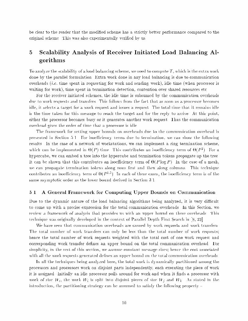
W = O(PpW )or W = O(P 2)Thus isoe�ciency due to communication overheads is given by W � O(P 2). The term corre-sponding to accessing the shared variable TARGET remains unchanged, and is given byO(P 2 logP ).For isoe�ciency due to contention on shared bus, we have to balance the time for computation withthe total time required to process the required number of messages on the Ethernet. Since all mes-sages have to be sent sequentially, the total time for processing all messages is of the same orderas the total communication overhead. Thus, we have, W=P � O(PpW ) or W � O(P 4). Wecan see that this term clearly dominates the communication overhead term, therefore, the overallisoe�ciency for this case is given by W � O(P 4). This should be compared with the isoe�ciencyvalue of O(P 2 logP ), which we had obtained under the �xed message size assumption.From the above sample cases, it is evident that the cost of work transfer has a signi�cantbearing on the overall scalability of a given scheme on a given architecture. Thus, it becomes veryimportant to analyze the application area to determine what assumptions can be made on the sizeof the work transfer message.8 Experimental Results and DiscussionHere we report on the experimental evaluation of the eight schemes. All the experiments were doneon a second generation NcubeTM in the context of the Satis�ability problem [5]. The Satis�abilityproblem consists of testing the validity of boolean formulae. Such problems arise in areas such asVLSI design and theorem proving among others [2, 5]. The problem is \given a boolean formulacontaining binary variables in disjunctive normal form, �nd out if it is unsatis�able". The Davisand Putnam algorithm [5] presents a fast and e�cient way of solving this problem. The algorithmessentially works by performing a depth �rst search of the binary tree formed by true/false assign-ments to the literals. Thus the maximum depth of the tree cannot exceed the number of literals.The algorithm works as follows: select a literal, assign it a value true, remove all clauses where thisliteral appears in the non-negated form, remove the literal from all clauses where this appears inthe negated form. This de�nes a single forward step. Using this step, search through all literalsby assigning values true (as described) and false (invert the roles of the negated and non-negatedforms) until such time as either the clause set becomes satis�able or we have explored all possibleassignments. Even if a formula is unsatis�able, only a small subset of the 2n combinations possiblewill actually be explored. For instance, for a 65 variable problem, the total number of combinationspossible is 265 ( approximately 3:69� 1019) but only about 107 nodes are actually expanded in atypical problem instance. The search tree for this problem is highly pruned in a nonuniform fashionand any attempt to simply partition the tree statically results in extremely poor load balance.We implemented the Davis-Putnam algorithm, and incorporated the load balancing algorithmsdiscussed in Sections 4, and 6.1 and 6.2 into it. This program was run on several unsatis�ableinstances. By choosing unsatis�able instances, we ensured that the number of nodes expanded by23

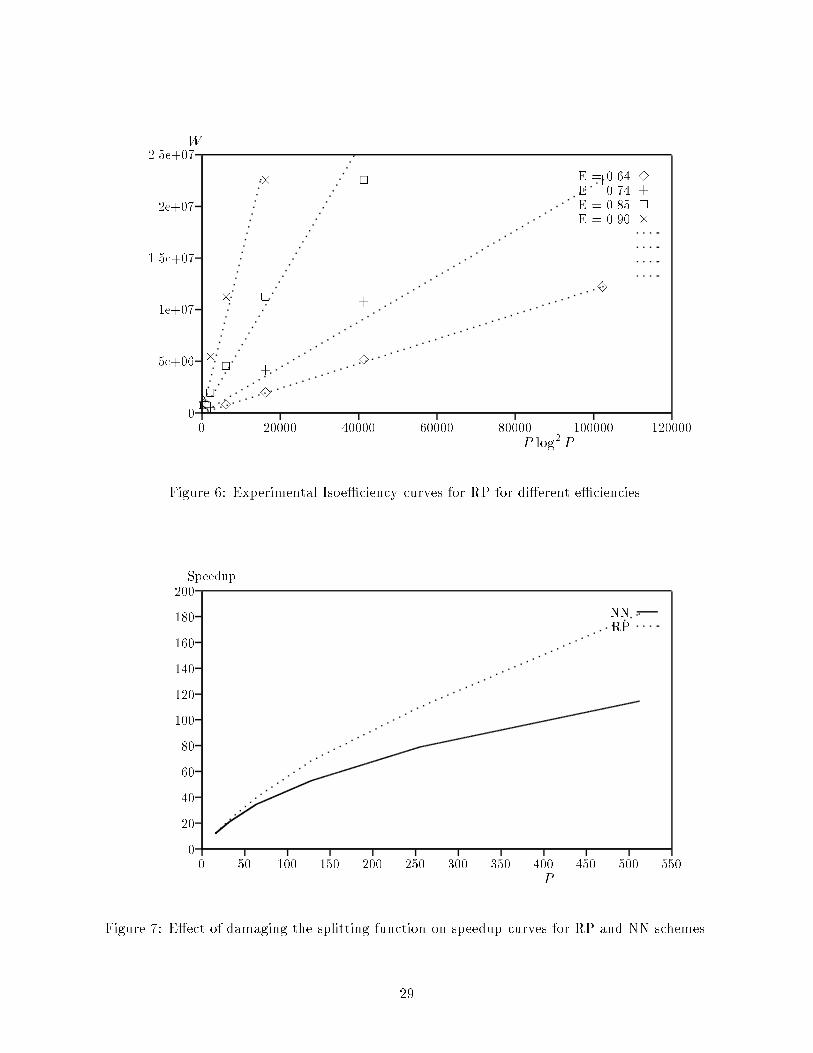
the parallel formulation was exactly the same as that by the sequential one, and any speedup losswas only due to the overheads of load balancing.In the various problem instances that the program was tested on, the total number of nodesin the tree varied between approximately 100 thousand and 10 million. The depth of the treegenerated (which is equal to the number of variables in the formula) varied between 35 and 65variables. The speedups were calculated with respect to the optimum sequential execution timefor the same problems. Average speedups were calculated by taking the ratio of the cumulativetime to solve all the problems in parallel using a given number of processors to the correspondingcumulative sequential time. On a given number of processors, the speedup and e�ciency werelargely determined by the tree size (which is roughly proportional to the sequential runtime).Thus, speedup on similar sized problems were quite similar.All schemes were tested over a sample set of 5 problem instances in the speci�ed size range.Tables 3 and 5 show average speedup obtained in parallel algorithm for solving the instances of thesatis�ability problem using eight di�erent load balancing techniques. Figures 8 and 8 present graphscorresponding to the speedups obtained. Graphs corresponding to NN and SB schemes have notbeen drawn. This is because they are nearly identical to RP and GRR schemes respectively. Table4 presents the total number of work requests made in the case of random polling and messagecombining for a speci�c problem. Figure 8 presents the corresponding graph and compares thenumber of messages generated with O(P log2 P ) and O(P logP ) for random polling and messagecombining respectively.Our analysis had shown that GRR-M has the best isoe�ciency for the hypercube architecture.However, the reader would note that even though the message combining scheme results in thesmallest number of requests, the speedup obtained is similar to that for RP. This is because softwaremessage combining on Ncube/2TM is quite expensive, and, this di�erence between the number ofwork requests made in load balancing schemes is not high enough. It is clear from the analysisin Section 5 and the trend in our experimental results, that this di�erence will widen for moreprocessors. Hence for larger number of processors, message combining scheme would eventuallyoutperform the other schemes. In the presence of message combining hardware, the log factorreduction in the number of messages causes a signi�cant reduction in overheads and consequentlythis scheme can be expected to perform better than the others even for a moderate number ofprocessors.Experimental results show that NN performs slightly better than RP. Recall that the isoef-�ciency of NN is �(P r), where r is determined by the quality of the splitting function (bettersplitting functions result in smaller values of r). In the context of the 15 puzzle, in [29], r wasdetermined to be 1.57. For up to 1024 processors, NN and RP have very similar performance.However, for higher values of P , P log2 P would become smaller than P r and RP would outperformNN. The exact crossover point is determined by the value of r, which depends on the quality ofthe splitting function. Appendix B analyzes the e�ect of the quality of the splitting function onoverall scalability of NN and RP. It is shown that the scalability of the NN scheme degrades muchfaster than RP as the quality of the splitting function deteriorates. Thus for domains where goodsplitting functions are not available, RP would be uniformly better than NN.To clearly demonstrate the e�ect of quality of splitting function on the scalability of RP andNN, we test the e�ect of damaging the splitting function on both of these schemes. Figure 824

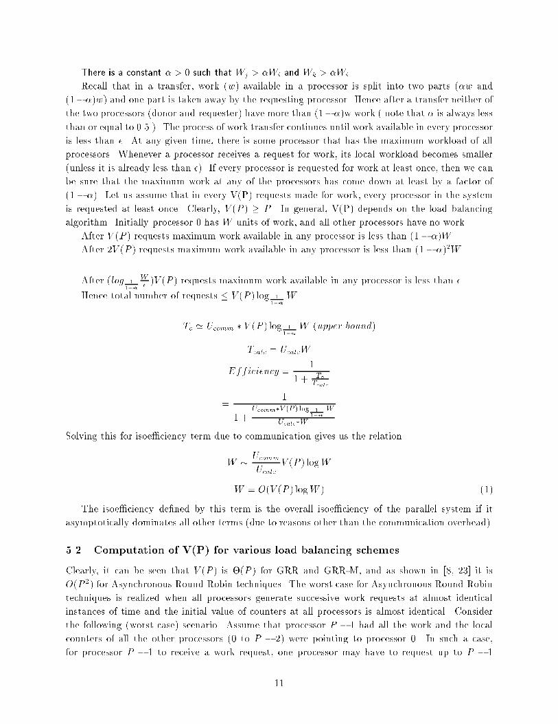
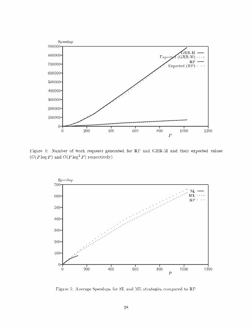
shows the experimental results comparing the speedup curves for RP and NN schemes with adamaged splitting function. It can be seen here that though with the original splitting function,NN marginally outperformed RP, it performs signi�cantly worse for poorer splitting functions. Thisis in perfect conformity with expected theoretical results.From our experiments, we observe that the performance of GRR and SB load balancing schemesis very similar. As shown analytically, both of these schemes have identical isoe�ciency functions.Since the isoe�ciency of these schemes is O(P 2 logP ), performance of these schemes deterioratesvery rapidly after 256 processors. Good speedups can be obtained for P > 256, only for very largeproblem instances. Neither of these schemes is thus useful for larger systems. Our experimentalresults also show ARR (Asynchronous Round Robin) to be more scalable than these two schemes,but signi�cantly less scalable than RP, NN or GRR-M. The readers should note that although theisoe�ciency of ARR is O(P 2 log2 P ) and that of GRR is O(P 2 log P ), ARR performs better thanGRR. The reason for this is that P 2 log2 P is only an upper bound which is derived using V (P ) =O(P 2). This value of V (P ) is only a loose upper bound for ARR. In contrast, the value of V (P )used for GRR (�(P )) is a tight bound.For the case of sender initiated load balancing, (SL and ML) the cuto� depths have been �ne-tuned for optimum performance. ML is implemented for l = 2, as for less than 1024 processorsl = 3 does not provide any improvements. It is clear from the speedup results presented in Table5 that the single level load balancing scheme has a very poor scalability. Though this schemeoutperforms the multilevel load balancing scheme for small number of processors, the subtaskgeneration bottleneck sets in for larger number of processors and performance degradation of singlelevel scheme is rapid after this point. The exact crossover point is determined by the problem size,values of parameters chosen and architecture dependent constants. Comparing the isoe�ciencyfunction for a two level load distribution, (given by �(P 32 (logP ) 32 )) with corresponding functionsfor RP and GRR-M which are given by O(P log3 P ) and O(P log2 P ), we see that, asymptotically,RP and GRR-M should both perform better than two level sender based distribution scheme. Ourexperimental results are thus in perfect conformity with expected analytical results.To demonstrate the accuracy of the isoe�ciency functions in Table 1, we experimentally verifythe isoe�ciency of the RP technique (the selection of this technique was arbitrary). As a part ofthis experiment, we ran 30 di�erent problem instances varying in size from 100 thousand nodesto 10 million nodes on a range of processors. Speedups and e�ciencies were computed for eachof these. Data points with same e�ciency for di�erent problem sizes and number of processorswere then grouped together. Where identical e�ciency points were not available, the problemsize was computed by averaging over points with e�ciencies in the neighborhood of the requiredvalue. This data is presented in Figure 8, which plots the problem size W against P log2 P forvalues of e�ciency equal to 0.9, 0.85, 0.74 and 0.64. Also note the two data points for which exactvalues of problem sizes are not available for corresponding e�ciencies. Instead we have plotted aneighboring point. We expect the points corresponding to the exact e�ciency to be collinear withthe others. We had seen in Section 5 that the isoe�ciency of the RP scheme was O(P log3 P ).We had further seen in Section 5.3.6 that due to large message startup time for the Ncube/2TM ,e�ective isoe�ciency of RP is O(P log2 P ) when P is not very large. Thus, analytically, the pointscorresponding to the same e�ciency on the said graph must be collinear. We can see from Figure8 that the points are indeed collinear, which clearly shows that the isoe�ciency of the RP scheme25

Scheme! ARR GRR-M RP NN GRR SBP#8 7.506 7.170 7.524 7.493 7.384 7.27816 14.936 14.356 15.000 14.945 14.734 14.51832 29.664 28.283 29.814 29.680 29.291 28.87564 57.721 56.310 58.857 58.535 57.729 57.025128 103.738 107.814 114.645 114.571 110.754 109.673256 178.92 197.011 218.255 217.127 184.828 184.969512 259.372 361.130 397.585 397.633 155.051 162.7981024 284.425 644.383 660.582 671.202Table 3: Average Speedups for Receiver Initiated Load Balancing strategies.Scheme! GRR-M RPP#8 260 56216 661 201332 1572 510664 3445 15060128 8557 46056256 17088 136457512 41382 3826951024 72874 885872Table 4: Number of requests generated for GRR-M and RP.is indeed what was theoretically derived. This demonstrates that it is indeed possible to accuratelyestimate the isoe�ciency of a parallel algorithm and establishes its viability as a useful tool inevaluating parallel system.9 Summary of Results and Future WorkThe scalability analysis of various load balancing schemes has provided valuable insights into therelative performance and suitability of these schemes for di�erent architectures.For the hypercube, our analysis shows that GRR-M, RP and NN schemes are more scalablethan ARR, GRR and SB; hence, they are expected to perform better for higher number of pro-cessors. Asymptotically, GRR-M has the best isoe�ciency of the three; but in the absence ofmessage combining hardware, the high constant of proportionality can cause GRR-M to performpoorer than RP and NN for moderate number of processors. In our experiments, GRR-M performssimilar to RR and NN for up to 1024 processors on the Ncube/2TM which does not have message26

Scheme! RP SL MLP#8 7.524 7.510 7.31516 15.000 14.940 14.40632 29.814 29.581 28.24664 58.857 52.239 56.003128 114.645 79.101 106.881256 218.255 192.102512 397.585 357.5151024 660.582 628.801Table 5: Speedups for Sender Initiated Load Balancing strategies in comparison to RP.

01002003004005006007000 200 400 600 800 1000 1200

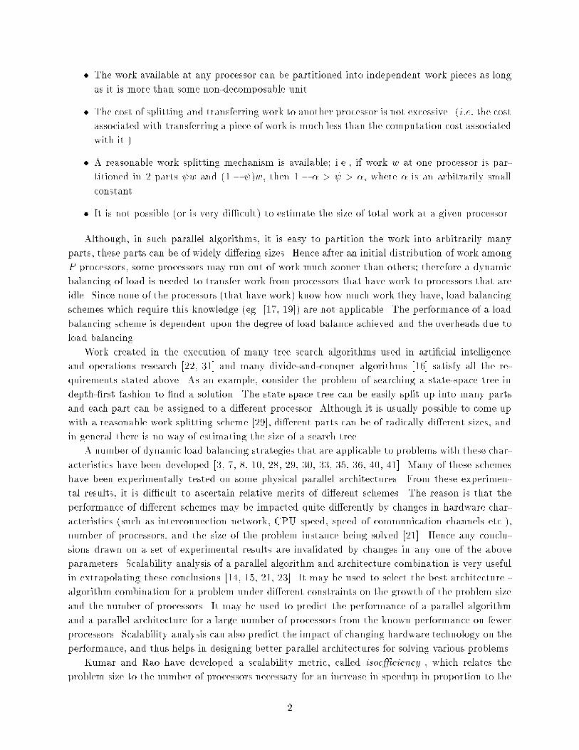
SpeedupP

ARRGRRGRR-MRPFigure 3: Average Speedups for Receiver Initiated Load Balancing Strategies.27

01000002000003000004000005000006000007000008000009000000 200 400 600 800 1000 1200

SpeedupP

GRR-MExpected (GRR-M)RPExpected (RP)Figure 4: Number of work requests generated for RP and GRR-M and their expected values(O(P log P ) and O(P log2 P ) respectively).

01002003004005006007000 200 400 600 800 1000 1200

SpeedupP

SLMLRPFigure 5: Average Speedups for SL and ML strategies compared to RP.28

05e+061e+071.5e+072e+072.5e+070 20000 40000 60000 80000 100000 120000

WP log2 P

E = 0.64 33 3 3 3E = 0.74 +

+ + + +E = 0.85 222 2 2 2 E = 0.90 ���� �

�Figure 6: Experimental Isoe�ciency curves for RP for di�erent e�ciencies.

0204060801001201401601802000 50 100 150 200 250 300 350 400 450 500 550

SpeedupP

NNRPFigure 7: E�ect of damaging the splitting function on speedup curves for RP and NN schemes.29

combining hardware. However, from the number of communication messages, it can be inferredthat, asymptotically, as P grows, GRR-M can eventually be expected to outperform RP and NNeven on the Ncube/2TM . Between RP and NN, RP has an asymptotically better scalability. Thus,with increasing number of processors, RP is expected to outperform NN. RP is also relativelyinsensitive to degradation of work splitting functions compared to NN. In our experiments, NNhas been observed to perform slightly better than RP. This is attributed to the high quality ofthe splitting function and the moderate number of processors. Our experiments show that with apoorer splitting function, NN performs consistently poorer than RP even for very small number ofprocessors.Scalability analysis indicates that SB has a performance similar to that of GRR even though SBgenerates fewer work requests by not requesting any processors that are known to be idle. The poorscalability of both of these schemes indicates that neither of these are e�ective for larger numberof processors. These conclusions have been experimentally validated.The sender based scheme, ML, has been shown to have reasonable scalability, and has only aslightly worse performance compared to RP in our experiments. A major drawback of this scheme isthat it requires the �ne tuning of a number of parameters to obtain best possible performance. Therandom allocation scheme for the hypercube presented in [33] has an isoe�ciency of O(P logP ),which is optimal. However, for many problems, the maximum obtainable e�ciency of this schemehas an upper bound much less than 1. This bound can be improved, and made closer to 1 by usinge�ective methods for granularity control; but it is not clear if such mechanisms can be derived forpractical applications. Also the memory requirements of these schemes are not well understood.In contrast, the best known receiver initiated scheme for the hypercube has an isoe�ciency ofO(P log2 P ), and its per-processor memory requirement is the same as that for corresponding serialimplementations.All the sender initiated schemes analyzed here use a di�erent work transfer mechanism comparedto the receiver initiated schemes. For instance, in the context of tree search, sender based schemesgive the current state itself as a piece of work, whereas stack splitting and transfer is the commonwork transfer mechanism for receiver initiated schemes. The sender-based transfer mechanismis more e�cient for problems for which the state description itself is very small but the stacksmay grow very deep and stack splitting may become expensive. In addition, if the machine hasa low message startup time (startup time component of the message passing time between twoprocessors), the time required to communicate a stack may become a sensitive function of the stacksize, which in turn may become large. In such domains, sender based schemes may potentiallyperform better than receiver based schemes.A network of workstations provides us with a cheap and universally available platform forparallelizing applications. Several applications have been parallelized to run on a small numberof workstations [1, 26]. For example, in [1] an implementation of parallel depth �rst branch andbound for VLSI oorplan optimization is presented. Linear speedups were obtained on up to 16processors. The essential part of this branch-and-bound algorithm is a scalable load balancingtechnique. Our scalability analysis can be used to investigate the viability of using a much largernumber of workstations for solving this problem. Recall that GRR has an overall isoe�ciency ofO(P 2 log P ) for this platform. Hence, if we had 1024 workstations on the network, we can obtainthe same e�ciency on a problem instance which is 10240 times bigger compared to a problem30

instance being run on 16 processors (10240 = 10242 log 1024162 log 16 ). This result is of signi�cance, as itindicates that it is indeed possible to obtain good e�ciencies with large number of workstations.Scalability analysis also sheds light on the degree of scalability of such a system with respect toother parallel architectures such as hypercube and mesh multicomputers. For instance, the bestapplicable technique implemented on a hypercube has an isoe�ciency function ofO(P log2 P ). Withthis isoe�ciency, we would be able to get identical e�ciencies as those obtained on 16 processorsby increasing the problem size 400 fold (which is 1024log2 102416 log2 16 ). We can thus see that it is possibleto obtain good e�ciencies even with smaller problems on the hypercube. We can thus concludefrom isoe�ciency functions that the hypercube o�ers a much more scalable platform compared tothe network of workstations for this problem.For the mesh architecture, we have analytically shown GRR-M and RP to have the best scal-ability. These are given by O(P 1:5 logP ) and O(P 1:5 log2 P ) respectively. These �gures indicatethat these schemes are less scalable than their corresponding formulations for hypercube connectednetworks. However, it must be noted that GRR-M is within a log factor of the lower bound onisoe�ciency for mesh architectures, given by P 1:5. Thus this scheme is near optimal for mesharchitecture.Speedup �gures of individual load balancing schemes can change with technology dependentfactors such as the CPU speed, the speed of communication channels etc. These performancechanges can be easily predicted using isoe�ciency analysis. For instance, if each of the CPUs of aparallel processor were made faster by a factor of 10, then Ucomm=Ucalc would increase by a factorof 10. From our analysis in Section 5.1, we can see that we would have to increase the size of ourproblem instance by a factor of 10 to be able to obtain the same e�ciency. On the other hand,increasing communication speed by a factor of 10 would enable us to obtain the same e�ciencyon problem instances a tenth the size of the original problem size. This shows that the impactof changes in technology dependent factors is moderate. These can, however, be quite drastic forother algorithms such as FFT [13] and Matrix algorithms [12]. Being able to make such predictionsis one of the signi�cant advantages of isoe�ciency analysis.Two problem characteristics, communication coupling between subtasks and the ability to es-timate work size, de�ne a spectrum of application areas. Di�erent load balancing strategies areneeded for di�erent points in this spectrum. In this paper, we have analyzed the point where thereis no communication coupling and its not possible to estimate work size. It would be interesting toinvestigate optimal load balancing schemes for other points in this spectrum. For instance, there isanother class of problems where the amount of work associated with a subtask can be determinedbut there is a very de�nite pattern of communication between subtasks. Examples can be found inscienti�c computations involving the solution of partial di�erential equations.Dynamic load Balancing algorithms for SIMD processors are of a very di�erent nature comparedto those for MIMD architectures [9, 27, 32, 18]. Due to architectural constraints in SIMD machines,load balancing needs to be done on a global scale. In contrast, on MIMD machines, load can bebalanced among a small subset of processors while the others are busy doing work. Further, inmassively parallel SIMD machines, computations are of a �ne granularity, hence communication tocomputation tradeo�s are very di�erent compared to MIMD machines. Hence, the load balancingschemes developed for MIMD architectures may not perform well on SIMD architectures. Analysissimilar to that used in this paper has been used to understand the scalability of di�erent load31

balancing schemes for SIMD architectures and to determine best schemes [18].Appendix AAnalysis of Load Balancing Algorithms for Mesh ArchitecturesHere we analyze the isoe�ciency function for the above schemes on the mesh architecture.Asynchronous Round RobinAs before, for this case, V (P ) = O(P 2). Ucomm for this architecture is �(pP ). Substituting these values of Ucommand V (P ) into Equation 1, the isoe�ciency for this scheme is given by O(P 2:5 log P ).Global Round RobinFor isoe�ciency due to communication overhead, V (P ) = O(P ) and Ucomm = �(pP ). Substituting these values intoEquation 1, the isoe�ciency due to communication overheads is O(P 1:5 log P ).For isoe�ciency due to contention, as discussed before, we need to equate the work at each processor (assuminge�cient distribution) with number of messages that need to be processed by processor 0 during this time. Thus forisoe�ciency, WP � V (P ) logWor WP � P logWSolving this equation for isoe�ciency, we getW = O(P 2 log P )Thus since the isoe�ciency due to contention asymptotically dominates the isoe�ciency due to communicationoverhead, the overall isoe�ciency is given by O(P 2 log P ).GRR-MFrom Section 5.2, we have V (P ) = �(P ). Also, message combining can be performed by propagating a work requestleft up to column 0 of the mesh and then propagating it up to processor 0. In this way, each increment on the variableTARGET takes �(�pP ), where � is the time allowed for message combining at each intermediate processor. Thus,Ucomm = �(�pP ).Substituting these values into Equation 1, the isoe�ciency due to communication overheads isO(P 1:5 log P ). Since we have no contention this term de�nes the overall isoe�ciency of this scheme.Random Polling on a MeshAs before, V (P ) = �(P log P ) and Ucomm = �(pP ). Substituting these values of Ucomm and V (P ) into Equation 1,this scheme has an isoe�ciency function of O(P 1:5 log2 P ).Appendix BE�ect of Quality of Splitting Function on Scalability.Our theoretical analysis shows that the isoe�ciency functions for RP and NN schemes are O(P log 11�� P � log22 P )and (P log2 1+ 1�2 ) respectively. 32

For RP, thus, W � O(P log 11�� P � log22 P )� O(P log2 Plog2 11�� P � log22 P )Now, 11� � = 1 + �+ �2 + ::::and for � << 1, 11�� � 1 + �. Substituting in relation for W, we get,W � O(P log2 Plog2(1 + �) � log22 P )Also, loge(1 + �) = �� �22 + �33 :::Again, for � << 1, we can neglect higher powers of �, andloge(1 + �) � �Substituting in relation for W, we get, W � O( 1� � P log3 P ) (4)Similarly, for the case of NN, W � (P log2 1+ 1�2 )� (P log2 2�( 1+ 1�4 ))� (P 1+log2( 1+ 1�4 ))� (P � P log2( 1+ 1�4 ))Thus we get W � (P � P log2 1��2) (5)Now consider Equations 4 and 5. On damaging the splitting function so as to reduce � by a factor of 2, isoe�ciencyfor RP increases by a factor of 2 whereas that for NN increases by a factor of P. This clearly demonstrates that thescalability of NN is signi�cantly degraded by a poor splitting function.AcknowledgementsThe authors sincerely acknowledge Dr. Robert Benner at Sandia National Labs for providing uswith access to the 1024 node Ncube/2TM . Vivek Sarin and Anshul Gupta provided many helpfulcomments on the earlier drafts of this paper. The idea of software message combining on thehypercube was suggested by Chuck Seitz. The authors also acknowledge the constructive commentsand suggestions by the referees.References[1] S. Arvindam, Vipin Kumar, and V. Nageshwara Rao. Floorplan optimization on multiprocessors. In Proceedingsof the 1989 International Conference on Computer Design (ICCD-89), 1989. Also published as MCC TechReport ACT-OODS-241-89.[2] S. Arvindam, Vipin Kumar, and V. Nageshwara Rao. E�cient parallel algorithms for search problems: Appli-cations in vlsi cad. In Proceedings of the Frontiers 90 Conference on Massively Parallel Computation, October1990. 33

[3] S. Arvindam, Vipin Kumar, V. Nageshwara Rao, and Vineet Singh. Automatic test pattern generation onmultiprocessors. Parallel Computing, 17, number 12:1323{1342, December 1991.[4] E. Charniak and D. McDermott. Introduction to Arti�cial Intelligence. Addison Wesley, 1985.[5] M. Davis, G. Logeman, and D. Loveland. A machine program for theorem proving. Communications of theACM, 5, number 7, 1962.[6] A. Gottlieb et al. The NYU ultracomputer - designing a MIMD, shared memory parallel computer. IEEETransactions on Computers, pages 175{189, February 1983.[7] Chris Ferguson and Richard Korf. Distributed tree search and its application to alpha-beta pruning. In Pro-ceedings of the 1988 National Conference on Arti�cial Intelligence, August 1988.[8] Raphael A. Finkel and Udi Manber. DIB - a distributed implementation of backtracking. ACM Trans. of Progr.Lang. and Systems, 9 No. 2:235{256, April 1987.[9] Roger Frye and Jacek Myczkowski. Exhaustive search of unstructured trees on the connection machine. InThinking Machines Corporation Technical Report, 1990.[10] M. Furuichi, K. Taki, and N. Ichiyoshi. A multi-level load balancing scheme for or-parallel exhaustive searchprograms on the multi-psi. In Proceedings of the 2nd ACM SIGPLAN Symposium on Principles and Practice ofParallel Programming, 1990. pp.50-59.[11] Ananth Grama, Vipin Kumar, and V. Nageshwara Rao. Experimental evaluation of load balancing techniquesfor the hypercube. In Proceedings of the Parallel Computing 91 Conference, 1991.[12] Anshul Gupta and Vipin Kumar. The scalability of Matrix Multiplication Algorithms on parallel computers.Technical Report TR 91-54, Computer Science Department, University of Minnesota, Minneapolis, MN 55455,1991.[13] Anshul Gupta and Vipin Kumar. The scalability of FFT on parallel computers. In Proceedings of the Frontiers90 Conference on Massively Parallel Computation, October 1990. An extended version of the paper will appearin IEEE Transactions on Parallel and Distributed Systems, 1993.[14] John L. Gustafson. Reevaluating Amdahl's Law. Communications of the ACM, 31(5):532{533, 1988.[15] John L. Gustafson, Gary R. Montry, and Robert E. Benner. Development of parallel methods for a 1024-processorhypercube. SIAM Journal on Scienti�c and Statistical Computing, 9 No. 4:609{638, 1988.[16] Ellis Horowitz and Sartaj Sahni. Fundamentals of Computer Algorithms. Computer Science Press, Rockville,Maryland, 1978.[17] L. V. Kale. Comparing the performance of two dynamic load distribution methods. In Proceedings of Interna-tional conference on Parallel Processing, pages 8{12, 1988.[18] George Karypis and Vipin Kumar. Unstructured Tree Search on SIMD Parallel Computers. Technical Report92{21, Computer Science Department, University of Minnesota, 1992. A short version of this paper appears inthe Proceedings of Supercomputing 1992 Conference, November 1992.[19] R. Keller and F. Lin. Simulated performance of a reduction based multiprocessor. IEEE Computers, July 19841984.[20] Kouichi Kimura and Ichiyoshi Nobuyuki. Probabilistic analysis of the e�ciency of the dynamic load distribution.In Proceedings of 1991 Distributed Memory and Concurrent Computers, 1991.[21] Vipin Kumar and Anshul Gupta. Analyzing the scalability of parallel algorithms and architectures: A survey.In Proceedings of the 1991 International Conference on Supercomputing, June 1991. also appear as an invitedpaper in the Proc. of 29th Annual Allerton Conference on Communuication, Control and Computing, Urbana,IL,October 1991.[22] Vipin Kumar, Dana Nau, and Laveen Kanal. General branch-and-bound formulation for and/or graph and gametree search. In Laveen Kanal and Vipin Kumar, editors, Search in Arti�cial Intelligence. Springer-Verlag, NewYork, 1988.[23] Vipin Kumar and V. Nageshwara Rao. Parallel depth-�rst search, part II: Analysis. International Journal ofParallel Programming, 16 (6):501{519, 1987. 34

[24] Vipin Kumar and V. Nageshwara Rao. Load balancing on the hypercube architecture. In Proceedings of the1989 Conference on Hypercubes, Concurrent Computers and Applications, pages 603{608, 1989.[25] Vipin Kumar and Vineet Singh. Scalability of Parallel Algorithms for the All-Pairs Shortest Path Problem: ASummary of Results. In Proceedings of the International Conference on Parallel Processing, 1990. Extended ver-sion appears in Journal of Parallel and Distributed Processing (special issue on massively parallel computation),Volume 13, 124-138, 1991.[26] Kai Li. Ivy: A shared virtual memory system for parallel computing. In Proceedings of International conferenceon Parallel Processing: Vol II, pages 94{101, 1988.[27] A. Mahanti and C. Daniels. Simd parallel heuristic search. To appear in Arti�cial Intelligence, 1992.[28] B. Monien and O. Vornberger. Parallel processing of combinatorial search trees. In Proceedings of InternationalWorkshop on Parallel Algorithms and Architectures, May 1987.[29] V. Nageshwara Rao and Vipin Kumar. Parallel depth-�rst search, part I: Implementation. International Journalof Parallel Programming, 16 (6):479{499, 1987.[30] Srinivas Patil and Prithviraj Banerjee. A parallel branch and bound algorithm for test generation. In IEEETransactions on Computer Aided Design, Vol. 9, No. 3, March 1990.[31] Judea Pearl. Heuristics - Intelligent Search Strategies for Computer Problem Solving. Addison-Wesley, Reading,MA, 1984.[32] C. Powley, R. Korf, and C. Ferguson. Ida* on the connection machine. To appear in Arti�cial Intelligence, 1992.[33] Abhiram Ranade. Optimal speedup for backtrack search on a butter y network. In Proceedings of the ThirdACM Symposium on Parallel Algorithms and Architectures, 1991.[34] S. Ranka and S. Sahni. Hypercube Algorithms for Image Processing and Pattern Recognition. Springer-Verlag,New York, 1990.[35] Vikram Saletore and L. V. Kale. Consistent linear speedup to a �rst solution in parallel state-space search. InProceedings of the 1990 National Conference on Arti�cial Intelligence, pages 227{233, August 1990.[36] Wei Shu and L. V. Kale. A dynamic scheduling strategy for the chare-kernel system. In Proceedings of Super-computing 89, pages 389{398, 1989.[37] Vineet Singh, Vipin Kumar, Gul Agha, and Chris Tomlinson. Scalability of parallel sorting on mesh multicom-puters. International Journal of Parallel Programming, 20 (2), 1991. A short version of this paper appears inthe Proceedings of the Fifth International Parallel Processing Symposium, 1991.[38] Douglas R. Smith. Random trees and the analysis of branch and bound proceedures. Journal of the ACM, 31No. 1, 1984.[39] Nageshwara Rao Vempaty, Vipin Kumar, and Richard Korf. Analysis of heuristic search algorithms. In Pro-ceedings of the National Conf. on Arti�cial Intelligenc e (AAAI-91), 1991.[40] Benjamin W. Wah, G.J. Li, and C. F. Yu. Multiprocessing of combinatorial search problems. IEEE Computers,June 1985 1985.[41] Benjamin W. Wah and Y.W. Eva Ma. Manip - a multicomputer architecture for solving combinatorial extremum-search problems. IEEE Transactions on Computers, c{33, May 1984.[42] Jinwoon Woo and Sartaj Sahni. Hypercube computing : connected components. Journal of Supercomputing,1991.[43] Jinwoon Woo and Sartaj Sahni. Computing biconnected components on a hypercube. Journal of Supercomputing,June 1991. 35