UNIVERSITY OF CALIFORNIA Santa Barbara Scalable Graph Algorithms in a High-Level Language Using Primitives Inspired by Linear Algebra A Dissertation submitted in partial satisfaction of the requirements for the degree of Doctor of Philosophy in Computer Science by Adam Lugowski Committee in Charge: Professor John R. Gilbert, Chair Professor Ben Zhao Professor Xifeng Yan September 2014

Welcome message from author
This document is posted to help you gain knowledge. Please leave a comment to let me know what you think about it! Share it to your friends and learn new things together.
Transcript
UNIVERSITY OF CALIFORNIASanta Barbara
Scalable Graph Algorithms in a High-LevelLanguage Using Primitives Inspired by Linear
Algebra
A Dissertation submitted in partial satisfactionof the requirements for the degree of
Doctor of Philosophy
in
Computer Science
by
Adam Lugowski
Committee in Charge:
Professor John R. Gilbert, Chair
Professor Ben Zhao
Professor Xifeng Yan
September 2014
The Dissertation ofAdam Lugowski is approved:
Professor Ben Zhao
Professor Xifeng Yan
Professor John R. Gilbert, Committee Chairperson
September 2014
Scalable Graph Algorithms in a High-Level Language Using Primitives Inspired
by Linear Algebra
Copyright © 2014
by
Adam Lugowski
iii
To my supportive parents and Nupur.
iv
Acknowledgements
I’m very grateful to be able to do my dissertation work at a great institution
like UCSB.
I’d especially like to thank my advisor, John Gilbert. His patience and superb
mentorship taught me the art and science of research. His masterful command of
the English language taught me the value of good presentation. I’m also grateful
for his willingness to mark up endless drafts of papers and theses with his signature
purple pen.
I also wish to thank my committee, Ben Zhao and Xifeng Yan. They have
provided me with valuable feedback that helped guide my research in the right
direction.
Many thanks also go to Aydın Buluç, who provided me with a great base
to work from, and for his ongoing support in making the KDT project possible.
Similarly, I want to thank Steve Reinhardt for his collaboration on KDT. His
insights, patience, and skill were invaluable on the KDT project. I owe a debt to
Shoaib Kamil and Armando Fox, for bringing their insights, direction, code, and
ideas to make the KDT and SEJITS integration work possible.
I also wish to thank Leonid Oliker, Sam Williams, and Aydın Buluç for giving
me the opportunity to intern at Lawrence Berkeley National Lab. It’s an honor
to work on our projects at that prestigious institution.
v
The help of David Mizell, Steve Reinhardt and my labmate Kevin Deweese
were instrumental in making our iterative algorithm in SPARQL work possible.
Research is a group effort; in that vein the lab discussions, collaborations, and
general support from my current and former lab mates proved invaluable. I thank
Aydın, Varad Deshmukh, Kevin Deweese, Veronika Strnadova, Victor Amelkin,
and Viral Shah for that.
Many people also helped with the less visible tasks that made my dissertation
work possible. I wish to thank Paul Weakliem, Jason Riedy, Stefan Boeriu, and
the staff at NERSC for help in getting access to the various machines that my
work benefitted from. I’d also like to thank the fine staff from the Computer
Science department office for making the administrative tasks so easy.
Finally I wish to thank my fellow graduate students for making these years
such a joy.
vi

Curriculum Vitæ
Adam Lugowski
Education
2012 Master of Science in Computer Science, UC Santa Barbara
2006 Bachelor of Science in Computer Science and Mathematics, Purdue
University
Experience
2009-2014 Graduate Research Assistant, UC Santa Barbara
2012 Summer Intern, Lawrence Berkeley National Labs
2005 Interns for Indiana (IFI) intern, Seyet LLC
2005 Interns for Indiana (IFI) intern, Vasc-Alert LLC
2004 Intern, Caterpillar Inc.
2003-2004 Intern, Delphi-Delco Verification Lab
2003 Undergraduate TA, Purdue University
2001-2003 Intern, Micro Data Base Systems
Selected Publications
Adam Lugowski, David Alber, Aydõn BuluŊ, John R Gilbert,
Steve Reinhardt, Yun Teng and Andrew Waranis: “A Flexible
vii
Open-Source Toolbox for Scalable Complex Graph Analysis", In
Proceedings of the Twelfth SIAM International Conference on
Data Mining (SDM12), April 2012.
Adam Lugowski, Aydõn BuluŊ, John Gilbert and Steve Rein-
hardt: “Scalable Complex Graph Analysis with the Knowledge
Discovery Toolbox", In IEEE International Conference on Acous-
tics, Speech, and Signal Processing (ICASSP), March 2012.
Aydõn BuluŊ, Erika Duriakova, Armando Fox, John R Gilbert,
Shoaib Kamil, Adam Lugowski, Leonid Oliker and Samuel Williams:
“High-Productivity and High-Performance Analysis of Filtered
Semantic Graphs", In 27th IEEE International Symposium on
Parallel and Distributed Processing (IPDPS 2013), May 2013.
Kevin Deweese, John R Gilbert, Adam Lugowski and Steve Rein-
hardt: “Graph Clustering in SPARQL", In SIAM Workshop on
Network Science, 2013.
Robert W. Techentin, Barry K. Gilbert, Adam Lugowski, Kevin
Deweese, John R. Gilbert, Eric Dull, Mike Hinchey, Steven P.
Reinhardt: “Implementing Iterative Algorithms with SPARQL",
In EDBT/ICDT Workshops, 2014.
viii
Adam Lugowski, John R Gilbert: “Efficient Sparse Matrix-Matrix
Multiplication on Multicore Architectures", In Sixth SIAM Work-
shop on Combinatorial Scientific Computing (CSC14), July 2014.
Adam Lugowski, Shoaib Kamil, Aydõn BuluŊ, Samuel Williams,
Erika Duriakova, Leonid Oliker, Armando Fox, John R. Gilbert:
“Parallel Processing of Filtered Queries in Attributed Semantic
Graphs", Accepted to JPDC.
ix
Abstract
Scalable Graph Algorithms in a High-Level LanguageUsing Primitives Inspired by Linear Algebra
Adam Lugowski
This dissertation advances the state of the art for scalable high-performance
graph analytics and data mining using the language of linear algebra. Many
graph computations suffer poor scalability due to their irregular nature and low
operational intensity. A small but powerful set of linear algebra primitives that
specifically target graph and data mining applications can expose sufficient coarse-
grained parallelism to scale to thousands of processors.
In this dissertation we advance existing distributed memory approaches in two
important ways. First, we observe that data scientists and domain experts know
their analysis and mining problems well, but suffer from little HPC experience. We
describe a system that presents the user with a clean API in a high-level language
that scales from a laptop to a supercomputer with thousands of cores. We utilize a
Domain-Specific Embedded Language with Selective Just-In-Time Specialization
to ensure a negligible performance impact over the original distributed memory
low-level code. The high-level language enables ease of use, rapid prototyping,
and additional features such as on-the-fly filtering, runtime-defined objects, and
exposure to a large set of third-party visualization packages.
x
The second important advance is a new sparse matrix data structure and set of
algorithms. We note that shared memory machines are dominant both in stand-
alone form and as nodes in distributed memory clusters. This thesis offers the
design of a new sparse-matrix data structure and set of parallel algorithms, a
reusable implementation in shared memory, and a performance evaluation that
shows significant speed and memory usage improvements over competing pack-
ages. Our method also offers features such as in-memory compression, a low-cost
transpose, and chained primitives that do not materialize the entire intermediate
result at any one time. We focus on a scalable, generalized, sparse matrix-matrix
multiplication algorithm. This primitive is used extensively in many graph algo-
rithms such as betweenness centrality, graph clustering, graph contraction, and
subgraph extraction.
Professor John R. Gilbert
Dissertation Committee Chair
xi
Contents
Acknowledgements v
Curriculum Vitæ vii
Abstract x
List of Figures xvi
List of Tables xxii
1 Introduction 11.1 The Landscape of Graph Analytics . . . . . . . . . . . . . . . . . 21.2 Graph Algorithms in the Language of Linear Algebra . . . . . . . 41.3 Outline of Thesis . . . . . . . . . . . . . . . . . . . . . . . . . . . 5
2 Basic Architecture of the Knowledge Discovery Toolbox 72.1 Introduction . . . . . . . . . . . . . . . . . . . . . . . . . . . . . . 72.2 Architecture and Context . . . . . . . . . . . . . . . . . . . . . . 122.3 Related Work . . . . . . . . . . . . . . . . . . . . . . . . . . . . . 152.4 Examples of use . . . . . . . . . . . . . . . . . . . . . . . . . . . . 16
2.4.1 Breadth-First Search . . . . . . . . . . . . . . . . . . . . . 172.4.2 Betweenness Centrality . . . . . . . . . . . . . . . . . . . . 222.4.3 PageRank . . . . . . . . . . . . . . . . . . . . . . . . . . . 262.4.4 Belief Propagation . . . . . . . . . . . . . . . . . . . . . . 292.4.5 Markov Clustering . . . . . . . . . . . . . . . . . . . . . . 312.4.6 Peer-Pressure Clustering . . . . . . . . . . . . . . . . . . . 322.4.7 Mini-workflow Example . . . . . . . . . . . . . . . . . . . 33
2.5 High Level Language Interface . . . . . . . . . . . . . . . . . . . . 35
xii
2.5.1 High Productivity for Graph Analysis . . . . . . . . . . . . 352.5.2 Organization of the Fundamental Classes . . . . . . . . . . 362.5.3 Semantic Graphs . . . . . . . . . . . . . . . . . . . . . . . 38
2.6 HPC Computational Engines . . . . . . . . . . . . . . . . . . . . 402.6.1 Combinatorial BLAS . . . . . . . . . . . . . . . . . . . . . 402.6.2 Evolution of KDT . . . . . . . . . . . . . . . . . . . . . . . 42
2.7 Conclusion . . . . . . . . . . . . . . . . . . . . . . . . . . . . . . . 43
3 Attributed Semantic Graphs and Filters 453.1 Introduction . . . . . . . . . . . . . . . . . . . . . . . . . . . . . . 453.2 Semantic Graph Example . . . . . . . . . . . . . . . . . . . . . . 453.3 KDT Design . . . . . . . . . . . . . . . . . . . . . . . . . . . . . . 483.4 Customizability: Supporting Attributes for Vertices and Edges . . 50
3.4.1 Datatypes . . . . . . . . . . . . . . . . . . . . . . . . . . . 503.4.2 Computation . . . . . . . . . . . . . . . . . . . . . . . . . 533.4.3 In-place Graph Filtering . . . . . . . . . . . . . . . . . . . 55
3.5 Performance . . . . . . . . . . . . . . . . . . . . . . . . . . . . . . 563.6 Conclusion . . . . . . . . . . . . . . . . . . . . . . . . . . . . . . . 57
4 Eliminating Python Callback Overhead with JIT Specialization 584.1 Introduction . . . . . . . . . . . . . . . . . . . . . . . . . . . . . . 584.2 Background . . . . . . . . . . . . . . . . . . . . . . . . . . . . . . 64
4.2.1 Filters As Scalar Semiring Operations . . . . . . . . . . . . 664.2.2 KDT Filters in Python . . . . . . . . . . . . . . . . . . . . 68
4.3 SEJITS Translation of Filters and Semiring Operations . . . . . . 744.3.1 Python Syntax for the DSLs . . . . . . . . . . . . . . . . . 754.3.2 Translating User-Defined Filters and Semiring Operations 774.3.3 Implementation in C++ . . . . . . . . . . . . . . . . . . . . 80
4.4 Attributes defined in Python and exposed to C++ . . . . . . . . . 824.4.1 Motivation . . . . . . . . . . . . . . . . . . . . . . . . . . . 824.4.2 Challenge . . . . . . . . . . . . . . . . . . . . . . . . . . . 834.4.3 Structure Declaration . . . . . . . . . . . . . . . . . . . . . 844.4.4 Memory Handling . . . . . . . . . . . . . . . . . . . . . . . 844.4.5 PDOs and SEJITS . . . . . . . . . . . . . . . . . . . . . . 854.4.6 Limitations . . . . . . . . . . . . . . . . . . . . . . . . . . 85
4.5 Experimental Design . . . . . . . . . . . . . . . . . . . . . . . . . 864.5.1 Algorithms Considered . . . . . . . . . . . . . . . . . . . . 864.5.2 Test Data Sets . . . . . . . . . . . . . . . . . . . . . . . . 874.5.3 Architectures . . . . . . . . . . . . . . . . . . . . . . . . . 90
4.6 A Roofline model of BFS . . . . . . . . . . . . . . . . . . . . . . . 91
xiii
4.7 Experimental Results . . . . . . . . . . . . . . . . . . . . . . . . . 974.7.1 Performance Effects of Permeability . . . . . . . . . . . . . 974.7.2 Performance Effects of Specialization . . . . . . . . . . . . 984.7.3 Parallel Scaling . . . . . . . . . . . . . . . . . . . . . . . . 1004.7.4 Performance on the Real Data Set . . . . . . . . . . . . . . 111
4.8 Results From Hardware Performance Counters . . . . . . . . . . . 1134.9 Related Work . . . . . . . . . . . . . . . . . . . . . . . . . . . . . 1194.10 Conclusion . . . . . . . . . . . . . . . . . . . . . . . . . . . . . . . 122
5 Shared Memory Sparse Matrix-Sparse Matrix Multiplication 1245.1 Introduction . . . . . . . . . . . . . . . . . . . . . . . . . . . . . . 1245.2 Quadtree Representation . . . . . . . . . . . . . . . . . . . . . . . 1255.3 Pair-List Matrix Multiplication Algorithm . . . . . . . . . . . . . 129
5.3.1 Symbolic Phase . . . . . . . . . . . . . . . . . . . . . . . . 1315.3.2 Symbolic Phase Example . . . . . . . . . . . . . . . . . . . 1345.3.3 Computational Phase . . . . . . . . . . . . . . . . . . . . . 1385.3.4 Post Processing . . . . . . . . . . . . . . . . . . . . . . . . 142
5.4 Choice of Division Threshold . . . . . . . . . . . . . . . . . . . . . 1435.5 Experiments and Comparisons . . . . . . . . . . . . . . . . . . . . 146
5.5.1 Experimental Design . . . . . . . . . . . . . . . . . . . . . 1465.5.2 Results . . . . . . . . . . . . . . . . . . . . . . . . . . . . . 1515.5.3 Code Comparisons . . . . . . . . . . . . . . . . . . . . . . 152
5.6 Discussion and Future Work . . . . . . . . . . . . . . . . . . . . . 1605.7 Conclusion . . . . . . . . . . . . . . . . . . . . . . . . . . . . . . . 162
6 Complex Graph Algorithms in a Database Query Language 1636.1 Introduction . . . . . . . . . . . . . . . . . . . . . . . . . . . . . . 1636.2 Our Selected Clustering Algorithm . . . . . . . . . . . . . . . . . 1646.3 Clustering Application . . . . . . . . . . . . . . . . . . . . . . . . 165
6.3.1 Datasets . . . . . . . . . . . . . . . . . . . . . . . . . . . 1656.3.2 Peer Pressure in SPARQL . . . . . . . . . . . . . . . . . . 1686.3.3 Discussion . . . . . . . . . . . . . . . . . . . . . . . . . . . 171
6.4 Workflow and Implementation . . . . . . . . . . . . . . . . . . . . 1726.4.1 Implementation in HTML/JavaScript . . . . . . . . . . . . 1726.4.2 Conversion Stage . . . . . . . . . . . . . . . . . . . . . . . 1736.4.3 Algorithm Stage . . . . . . . . . . . . . . . . . . . . . . . . 1756.4.4 Results Stage . . . . . . . . . . . . . . . . . . . . . . . . . 175
6.5 Results . . . . . . . . . . . . . . . . . . . . . . . . . . . . . . . . . 1766.5.1 Test Data . . . . . . . . . . . . . . . . . . . . . . . . . . . 1776.5.2 BTER Data . . . . . . . . . . . . . . . . . . . . . . . . . . 179
xiv
6.5.3 Smackdown Data . . . . . . . . . . . . . . . . . . . . . . . 1806.6 Conclusion . . . . . . . . . . . . . . . . . . . . . . . . . . . . . . . 181
7 Conclusions 182
Bibliography 183
Appendices 193
A QuadMat Experimental Data 194
B Systems 201B.1 Neumann . . . . . . . . . . . . . . . . . . . . . . . . . . . . . . . 201B.2 Mirasol . . . . . . . . . . . . . . . . . . . . . . . . . . . . . . . . . 201B.3 Hopper . . . . . . . . . . . . . . . . . . . . . . . . . . . . . . . . . 201B.4 Carver . . . . . . . . . . . . . . . . . . . . . . . . . . . . . . . . . 202
xv
List of Figures
2.1 An example graph analysis mini-workflow in KDT. . . . . . . . . 82.2 KDT code implementing the mini-workflow illustrated in Figure 2.1. 102.3 A notional iterative analytic workflow, in which KDT is used tobuild the graph and perform the complex analysis at steps 2 and 3. . . 112.4 The architecture of Knowledge Discovery Toolbox. The top-layermethods are primarily used by domain experts, and include centralityand cluster for semantic graphs. The middle-layer methods are pri-marily used by graph-algorithm developers to implement the top-layermethods. KDT is layered on top of Combinatorial BLAS. . . . . . . . 132.5 Two steps of breadth-first search, starting from vertex 7, usingsparse matrix-sparse vector multiplication with “max” in place of “+”. . 172.6 Speed comparison of the KDT and pure CombBLAS implemen-tations of Graph500. BFS was performed on a scale 29 input graphwith 500M vertices and 8B edges. The units on the vertical axis areGigaTEPS, or 109 traversed edges per second. The small discrepan-cies between KDT and CombBLAS are largely artifacts of the networkpartition granted to the job. KDT’s overhead is negligible. . . . . . . . 212.7 Performance comparison of KDT and PBGL breadth-first search.The reported numbers are in MegaTEPS, or 106 traversed edges persecond. The graphs are Graph500 RMAT graphs as described in the text. 232.8 Performance of betweenness centrality in KDT on synthetic power-law graphs (see Section 2.4.1). The units on the vertical axis are MegaTEPS,or 106 traversed edges per second. The black line shows ideal linear scal-ing for the scale 18 graph. The x-axis is in logarithmic scale. Our currentbackend requires a square number of processors. . . . . . . . . . . . . . 25
xvi
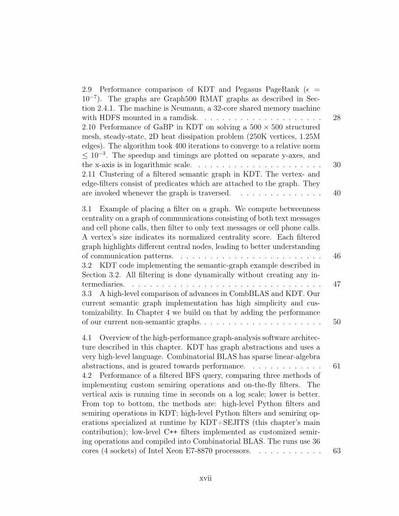
2.9 Performance comparison of KDT and Pegasus PageRank (ε =10−7). The graphs are Graph500 RMAT graphs as described in Sec-tion 2.4.1. The machine is Neumann, a 32-core shared memory machinewith HDFS mounted in a ramdisk. . . . . . . . . . . . . . . . . . . . . 282.10 Performance of GaBP in KDT on solving a 500 × 500 structuredmesh, steady-state, 2D heat dissipation problem (250K vertices, 1.25Medges). The algorithm took 400 iterations to converge to a relative norm≤ 10−3. The speedup and timings are plotted on separate y-axes, andthe x-axis is in logarithmic scale. . . . . . . . . . . . . . . . . . . . . . 302.11 Clustering of a filtered semantic graph in KDT. The vertex- andedge-filters consist of predicates which are attached to the graph. Theyare invoked whenever the graph is traversed. . . . . . . . . . . . . . . 40
3.1 Example of placing a filter on a graph. We compute betweennesscentrality on a graph of communications consisting of both text messagesand cell phone calls, then filter to only text messages or cell phone calls.A vertex’s size indicates its normalized centrality score. Each filteredgraph highlights different central nodes, leading to better understandingof communication patterns. . . . . . . . . . . . . . . . . . . . . . . . . 463.2 KDT code implementing the semantic-graph example described inSection 3.2. All filtering is done dynamically without creating any in-termediaries. . . . . . . . . . . . . . . . . . . . . . . . . . . . . . . . . 473.3 A high-level comparison of advances in CombBLAS and KDT. Ourcurrent semantic graph implementation has high simplicity and cus-tomizability. In Chapter 4 we build on that by adding the performanceof our current non-semantic graphs. . . . . . . . . . . . . . . . . . . . . 50
4.1 Overview of the high-performance graph-analysis software architec-ture described in this chapter. KDT has graph abstractions and uses avery high-level language. Combinatorial BLAS has sparse linear-algebraabstractions, and is geared towards performance. . . . . . . . . . . . . 614.2 Performance of a filtered BFS query, comparing three methods ofimplementing custom semiring operations and on-the-fly filters. Thevertical axis is running time in seconds on a log scale; lower is better.From top to bottom, the methods are: high-level Python filters andsemiring operations in KDT; high-level Python filters and semiring op-erations specialized at runtime by KDT+SEJITS (this chapter’s maincontribution); low-level C++ filters implemented as customized semir-ing operations and compiled into Combinatorial BLAS. The runs use 36cores (4 sockets) of Intel Xeon E7-8870 processors. . . . . . . . . . . . 63
xvii
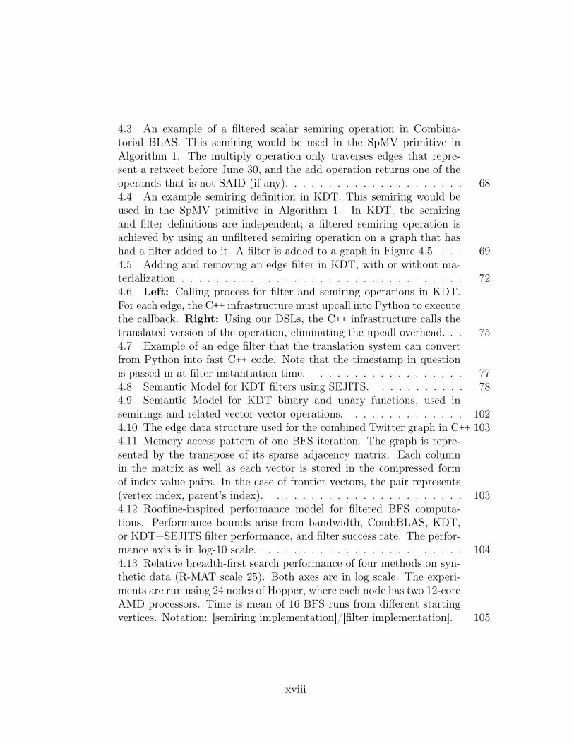
4.3 An example of a filtered scalar semiring operation in Combina-torial BLAS. This semiring would be used in the SpMV primitive inAlgorithm 1. The multiply operation only traverses edges that repre-sent a retweet before June 30, and the add operation returns one of theoperands that is not SAID (if any). . . . . . . . . . . . . . . . . . . . . 684.4 An example semiring definition in KDT. This semiring would beused in the SpMV primitive in Algorithm 1. In KDT, the semiringand filter definitions are independent; a filtered semiring operation isachieved by using an unfiltered semiring operation on a graph that hashad a filter added to it. A filter is added to a graph in Figure 4.5. . . . 694.5 Adding and removing an edge filter in KDT, with or without ma-terialization. . . . . . . . . . . . . . . . . . . . . . . . . . . . . . . . . . 724.6 Left: Calling process for filter and semiring operations in KDT.For each edge, the C++ infrastructure must upcall into Python to executethe callback. Right: Using our DSLs, the C++ infrastructure calls thetranslated version of the operation, eliminating the upcall overhead. . . 754.7 Example of an edge filter that the translation system can convertfrom Python into fast C++ code. Note that the timestamp in questionis passed in at filter instantiation time. . . . . . . . . . . . . . . . . . 774.8 Semantic Model for KDT filters using SEJITS. . . . . . . . . . . 784.9 Semantic Model for KDT binary and unary functions, used insemirings and related vector-vector operations. . . . . . . . . . . . . . 1024.10 The edge data structure used for the combined Twitter graph in C++ 1034.11 Memory access pattern of one BFS iteration. The graph is repre-sented by the transpose of its sparse adjacency matrix. Each columnin the matrix as well as each vector is stored in the compressed formof index-value pairs. In the case of frontier vectors, the pair represents(vertex index, parent’s index). . . . . . . . . . . . . . . . . . . . . . . 1034.12 Roofline-inspired performance model for filtered BFS computa-tions. Performance bounds arise from bandwidth, CombBLAS, KDT,or KDT+SEJITS filter performance, and filter success rate. The perfor-mance axis is in log-10 scale. . . . . . . . . . . . . . . . . . . . . . . . . 1044.13 Relative breadth-first search performance of four methods on syn-thetic data (R-MAT scale 25). Both axes are in log scale. The experi-ments are run using 24 nodes of Hopper, where each node has two 12-coreAMD processors. Time is mean of 16 BFS runs from different startingvertices. Notation: [semiring implementation]/[filter implementation]. 105
xviii
4.14 Relative maximal independent set performance of four methods onsynthetic data (Erdős-Rényi scale 22). y-axis uses a log scale. The runsuse 36 cores of Intel Xeon E7-8870 processors. Time is mean of 16 runs.Notation: [semiring implementation]/[filter implementation]. . . . . . . 1064.15 Parallel ‘strong scaling’ results of filtered BFS on Mirasol, withvarying filter permeability on a synthetic data set (R-MAT scale 22).Both axes are in log-scale, time is in seconds (mean of 16 runs from differ-ent starting vertices). Single core Python/Python and Python/SEJITSruns did not finish in a reasonable time to report. Notation: [semiringimplementation]/[filter implementation]. . . . . . . . . . . . . . . . . . 1074.16 Parallel ‘strong scaling’ results of filtered MIS on Mirasol, withvarying filter permeability on a synthetic data set (Erdős-Rényi scale22). Both axes are in log-scale, time is in seconds (mean of 16 runs).Notation: [semiring implementation]/[filter implementation]. . . . . . 1084.17 Parallel ‘strong scaling’ results of filtered BFS on Hopper, withvarying filter permeability on a synthetic data set (R-MAT scale 25).Both axes are in log-scale, time is in seconds (mean of 16 runs from dif-ferent starting vertices). Notation: [semiring implementation]/[filter im-plementation]. . . . . . . . . . . . . . . . . . . . . . . . . . . . . . . . . 1094.18 Parallel ‘weak scaling’ results of filtered BFS on Hopper, using 1%percent permeability. y-axis is in log scale, time is in seconds. From topto bottom, the methods are: high-level Python filters and semiring oper-ations in KDT; high-level Python filters and semiring operations special-ized at runtime by KDT+SEJITS; low-level C++ filters implemented ascustomized semiring operations and compiled into Combinatorial BLAS. 1104.19 Relative filtered breadth-first search performance of three methodson real Twitter data. The y-axis is in seconds on a log scale. The runsuse 16 cores of Intel Xeon E7-8870 processors. . . . . . . . . . . . . . . 1124.20 PAPI performance counters vs. time (in µs), showing (a) total in-structions, (b) L1 instruction cache misses, (c) L1 data cache misses, and(d) total L2 misses. BFS on Scale 22 graph with 100% permeable filter,repeated 16 times from starting vertex 1726462. P=9 on Mirasol. Eachpoint is a counter value for a single process in a single BFS iteration.Table 4.6 offers a summary of the same data in tabular form. . . . . . 1144.21 PAPI performance counters vs. time (in µs). BFS on Scale 22graph with 10% permeable filter, repeated 16 times from starting vertex1291427. P=9 on Mirasol. Each point is a counter value for a singleprocess in a single BFS iteration. Table 4.7 offers a summary of thesame data in tabular form. . . . . . . . . . . . . . . . . . . . . . . . . . 117
xix
5.1 Computation of a result block using a list of pairwise block multi-plications. . . . . . . . . . . . . . . . . . . . . . . . . . . . . . . . . . . 1265.2 Quadtree of an adjacency matrix of a power law graph. This ismatrix A in our running example in Figure 5.6. . . . . . . . . . . . . . 1285.3 Quadtree of an adjacency matrix of an Erdős-Rényi graph. This ismatrix B in our running example in Figure 5.6. . . . . . . . . . . . . . 1295.4 Illustration of Equation (5.3). . . . . . . . . . . . . . . . . . . . . 1325.5 Division mismatch: a leaf block is paired with an inner block. Ashadow subdivision of the leaf block yields an inner block that resolvesthe mismatch and allows another recursive step. . . . . . . . . . . . . . 1345.6 The running example. We wish to multiply an RMAT matrix withan adjacency matrix of an Erdős-Rényi graph. The quadtree for theRMAT is shown in Figure 5.2, and the ER in Figure 5.3. . . . . . . . . 1355.7 Example Trace I: The root symbolic task applies the recursive case.The next recursive symbolic task has a mix of inner block and leaves, soperforms a shadow subdivide. The next recursion are all leaf tasks, soare turned into compute tasks. . . . . . . . . . . . . . . . . . . . . . . 1365.8 Example Trace II: Trace that requires 3 levels of symbolic tasks. . 1375.9 Speedup compared to CSparse for CombBLAS and QuadMat on 1,4, 16, 36, and 64 threads. Y-axis is in log scale. Note that the machinehas 40 cores, so the 64 thread results are using multiple threads per core. 1525.10 Strong scaling of normal QuadMat. Each line shows the speedupfor a particular problem when more threads are used. . . . . . . . . . 1575.11 Strong scaling comparison of normal QuadMat with a special ver-sion with increased arithmetic intensity to show impact of memory ef-fects. . . . . . . . . . . . . . . . . . . . . . . . . . . . . . . . . . . . . 1585.12 Breakdown of time spent in each part of the algorithm on a singlecore. The green ‘SPA Arithmetic & Storage’ portion represents the in-ner block product computation. The blue ‘Column Organize’ proportionaccounts for the time to generate and combine column organizers. Thered ‘Symbolic Phase’ is dominated by shadow block creation. Miscel-laneous code such as destructors and TBB overhead go into the black‘Other’ portion. . . . . . . . . . . . . . . . . . . . . . . . . . . . . . . . 159
6.1 One iteration of the PeerPressure clustering algorithm. We haveincluded JavaScript references to graphName and i variables, which de-note the user’s choice of graph name and algorithm iteration, respectively. 1706.2 A query which creates “hasLink” edges between two rows of a tableif their Column 11 values are within 5 of each other. . . . . . . . . . . 174
xx
6.3 Sankey diagram visualization of clustering. Nodes on the left areindividual clusters (labeled with cluster ID, which is derived from arowID), nodes on the right are tables. The thickness of a link betweena cluster and a table is proportional to the number of rows of that tablein that cluster. . . . . . . . . . . . . . . . . . . . . . . . . . . . . . . . 1766.4 Query used for Sankey diagram. . . . . . . . . . . . . . . . . . . 1776.5 A screenshot of our SPARQL over HTTP webpage. Output foreach section is printed above each horizontal line. . . . . . . . . . . . . 178
A.1 FLOPS, or nonzero arithmetic operations per second, for each ofthe problems listed in Tables A.1 and A.2. Each set of five CombBLASand QuadMat bars correspond to 1, 4, 16, 36 and 64 threads, while theCSparse bar is a single thread. The machine has 40 cores capable of 80concurrent threads. The height of each bar indicates the mean of 5 runs;the error bars mark the fastest and slowest runs. . . . . . . . . . . . . 199
xxi
List of Tables
4.1 Overheads of using the filtering DSL. . . . . . . . . . . . . . . . . 814.2 Sizes (vertex and edge counts) of different combined twitter graphs. 894.3 Statistics about the largest strongly connected components of thetwitter graphs . . . . . . . . . . . . . . . . . . . . . . . . . . . . . . . . 894.4 Statistics about the filtered BFS runs on the R-MAT graph of Scale23 (M: million) . . . . . . . . . . . . . . . . . . . . . . . . . . . . . . . 954.5 Breakdown of the volume of data movement by memory accesspattern and operation. . . . . . . . . . . . . . . . . . . . . . . . . . . . 954.6 PAPI measurements for 100% filter, showing (Time_usec) totaltime, (TOT_INS) total instructions, (L1_ICM) L1 instruction cachemisses, (L1_DCM) L1 data cache misses, and (L2_TCM) total L2misses. All values are the mean of 96 points (9 processes × 16 repeats).Figure 4.20 is a visual representation of this data. . . . . . . . . . . . . 1154.7 PAPI measurements for 10% filter, showing (Time_usec) totaltime, (TOT_INS) total instructions, (L1_ICM) L1 instruction cachemisses, (L1_DCM) L1 data cache misses, and (L2_TCM) total L2misses. All values are the mean of 96 points (9 processes × 16 repeats).Figure 4.21 is a visual representation of this data. . . . . . . . . . . . . 116
5.1 Dataset categories. Each SpGEMM problem’s name specifies thematrix used and the operation. The matrix name is a concatenation ofBase, Scale, and RP from this table. The operation is denoted by asuffix from Section 5.5.1. . . . . . . . . . . . . . . . . . . . . . . . . . 149
A.1 The Problems - Matrix Squares. Colors in the visual representationof nonzero distribution indicate density. Green and red hues representmore nonzeros. All matrices here and in Table A.2 share the same colorscale. . . . . . . . . . . . . . . . . . . . . . . . . . . . . . . . . . . . . . 195
xxii
A.2 The Problems - Algebraic Multigrid Contractions, Permutations,and Submatrix Extractions. Colors in the visual representation of nonzerodistribution indicate density. Green and red hues represent more nonze-ros. All matrices here and in Table A.1 share the same color scale. . . . 196A.3 Matrix Square elapsed time in seconds, mean of 5 runs. The ma-chine has 40 cores capable of 80 concurrent threads. . . . . . . . . . . 197A.4 Algebraic Multigrid Contraction, Permutation, and Submatrix Ex-traction elapsed time in seconds, mean of 5 runs. The machine has 40cores capable of 80 concurrent threads. . . . . . . . . . . . . . . . . . 198A.5 Problem statistics extracted using an instrumented build of Quad-Mat run with one thread. Detailed analysis of this data is in Sec-tions 5.5.3 and 5.5.3. The division threshold is chosen to balance par-allelism with minimization of total block count (reduce hypersparseblocks). The same very preliminary choice algorithm is used for allproblems. Relatively poor QuadMat performance on some problems isexplained by two factors. Poor scaling can be due to insufficient poten-tial parallelism (threshold too large). Poor computational performance(torus squares, all permutations and submatrix extractions) is due tolow A organizer lookup utility (threshold too small). . . . . . . . . . . 200
xxiii
Chapter 1
Introduction
Analysis of very large graphs has become indispensable in fields ranging from
genomics and biomedicine to financial services, marketing, national security, and
many others. In many applications the requirements are moving beyond relatively
simple filtering and aggregation queries to complex graph algorithms involving
clustering, shortest-path searches, centrality, and so on. These complex graph
algorithms typically require high-performance computing resources to be feasible
on large graphs. However, users and developers of complex graph algorithms
are hampered by the lack of a flexible, scalable, reusable infrastructure for high-
performance computational graph analytics.
In this thesis we show that high performance computation on very large graphs
is enabled by efficient implementations of interfaces to algebraic primitives.
1
Chapter 1. Introduction
1.1 The Landscape of Graph Analytics
Many packages have answered the call for an HPC graph analysis toolkit.
Their approaches, scalability, and applicability vary significantly.
Pregel [78] wraps the “think like a vertex” principle in a bulk synchronous
model. In each iteration a vertex may send and receive messages to and from other
vertices, perform computation, and vote whether to halt. Pregel is an internal
Google project built with massive scale and fault-tolerance in mind. Giraph [7] is
an open source counterpart.
GraphLab [69] also follows the “think like a vertex” style. Users write vertex
code in a domain-specific language (DSL), while GraphLab handles the distribu-
tion between nodes and the parallelism. GraphLab is targeted at iterative sparse
graph algorithms in the machine learning domain.
LEMON [33] is a C++ template library that supplies graph concepts, methods
that operate on those concepts, and pre-made complete algorithms. LEMON is
powerful and is easy to learn, but it is purely sequential.
Java Universal Network/Graph framework (JUNG) [87] is a very flexible Java
graph library whose healthy set of algorithms and visualization tools make it a
good prototyping platform.
2
Chapter 1. Introduction
The sequential Boost Graph Library (BGL) [100] takes its inspiration from
the Standard Template Library. BGL recognizes that there is no one-size-fits-all
graph data structure, so it provides a variety of containers and algorithms that
work on abstract containers. The Parallel Boost Graph Library (PBGL) [50] is
a distributed memory extension of BGL that retains the latter’s large algorithm
library by building distributed variants of BGL’s containers.
Pegasus [55] is a package built on top of MapReduce that uses a primitive
similar to matrix-vector multiplication, called GIM-V. This primitive expresses
vertex-centered computations that combine data from neighboring edges and ver-
tices. Pegasus is a good fit when the graph is extracted from a MapReduce cloud,
at the cost of MapReduce’s significant overhead.
The MultiThreaded Graph Library (MTGL) [14] follows a design similar to the
PBGL, but with kernels written to take advantage of the massively multithreaded
Cray ThreadStorm processors used in the Cray XMT and Urika systems. The
MTGL introduces extremely parallel methods to traverse graphs which work very
well on the XMT, but may not translate to more conventional machines.
YarcData’s Urika [112] is a ThreadStorm-based dedicated SPARQL appliance
that provides a SQL-like query interface to search for patterns in very large graphs.
Urika takes advantage of the unique abilities of its processor to handle queries that
are very inefficient on conventional hardware.
3
Chapter 1. Introduction
1.2 Graph Algorithms in the Language of Linear
Algebra
Our work builds on the idea that linear-algebraic primitives provide a strong
foundation for scalable parallel graph algorithms.
Many traditional approaches to graph description and computation result in
algorithms that are limited by memory latency, with many cache misses and low
computational intensity. In contrast, the definitions of linear algebraic operations
provide natural paths to both partitioning of data and parallelizing computation.
More importantly, the well-structured data access patterns of linear algebraic
primitives allow code that is limited by bandwidth rather than latency [57].
The list of graph algorithms that have been implemented with linear alge-
braic primitives is long. It includes breadth first search [57], betweenness cen-
trality [24], shortest paths and spanning trees [57], peer pressure clustering [57],
PageRank [88], maximal independent set [57] (by variation of Luby’s algorithm [71]),
graph contraction [57], triangle counting [44], and triangle enumeration [45].
Formally, matrix and vector operations involve linear algebra over a semiring [46].
The most familiar semiring is the field of real numbers with the operations (+,×),
but there are many others. The choice of semiring is important to the implemen-
4
Chapter 1. Introduction
tation of graph algorithms in linear algebra. Some formulations use the (+,×)
semiring, some use the tropical (min,+), some use others.
Since graphs are rarely complete, sparse data structures and algorithms are
used to represent what is abstractly a 2-D adjacency array. We distinguish between
a sparse matrix (which is an algebraic object) and a sparse array (which is a data
structure). A sparse matrix algorithm can be implemented using a sparse array,
but a sparse array does not require existence of an explicit identity element and
allows mixing different semirings on the same data structure.
1.3 Outline of Thesis
The remaining chapters cover five significant contributions.
In Chapter 2, we describe the motivation for and architecture of the Knowledge
Discovery Toolbox (KDT) [72]. KDT’s main goal is to expose a scalable high-
performance infrastructure to Domain Experts, that is, people familiar with a
particular applied problem but who are not skilled high-performance computing
(HPC) programmers. Thus KDT has three main layers targeted at three distinct
groups. The foundation is laid by HPC Experts who are able to write scalable
and flexible primitives in a high-performance language. Algorithm Experts craft
5
Chapter 1. Introduction
algorithms using the exposed primitives in a high-productivity language. Finally,
Domain Experts use the algorithms to solve their problems.
Attributed semantic graphs are important in many workloads [?], but are dif-
ficult to express in traditional linear algebraic packages. In Chapter 3 we describe
KDT’s support for user-defined attributes, and the design of a powerful, flexi-
ble, and computationally inexpensive on-the-fly graph filtering system built on
predicates.
KDT’s primitive functions are customizable through a callback mechanism
that enables user-defined semirings and filter predicates, among many other uses.
Like the rest of KDT user code, these callbacks are written in a high-productivity
language. In Chapter 4 we describe our method to ensure that callbacks are not
a performance bottleneck.
In Chapter 5 we describe a new sparse matrix data structure called QuadMat,
and a shared-memory parallel sparse matrix-sparse matrix multiplication algo-
rithm. Sparse matrix multiplication forms the foundation of many graph algo-
rithms, but this work also has applications that go beyond graph algorithms.
SPARQL, as implemented in the Urika appliance, provides a very effective
way to perform local queries, while linear algebraic algorithms are particularly well
suited to calculating global metrics. In Chapter 6 we explore a method to compute
a global metric, PeerPressure clustering, using SPARQL as the underlying engine.
6
Chapter 2
Basic Architecture of theKnowledge Discovery Toolbox
This chapter is based on a paper published in SDM’12 [72].
2.1 Introduction
This chapter provides an introduction to the Knowledge Discovery Toolbox,
its architecture, and how it is meant to be used.
In many applications, the requirements for analysis of large graphs are moving
beyond relatively simple filtering and aggregation queries to complex graph al-
gorithms involving clustering (which may depend on machine learning methods),
shortest-path computations, and so on. These complex graph algorithms typically
require high-performance computing resources to be feasible on large graphs. How-
ever, users and developers of complex graph algorithms are hampered by the lack
7
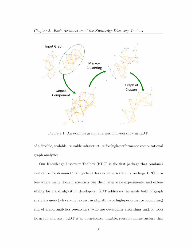
Chapter 2. Basic Architecture of the Knowledge Discovery Toolbox
Largest Component
Graph of Clusters
Markov Clustering
Input Graph
Figure 2.1: An example graph analysis mini-workflow in KDT.
of a flexible, scalable, reusable infrastructure for high-performance computational
graph analytics.
Our Knowledge Discovery Toolbox (KDT) is the first package that combines
ease of use for domain (or subject-matter) experts, scalability on large HPC clus-
ters where many domain scientists run their large scale experiments, and exten-
sibility for graph algorithm developers. KDT addresses the needs both of graph
analytics users (who are not expert in algorithms or high-performance computing)
and of graph analytics researchers (who are developing algorithms and/or tools
for graph analysis). KDT is an open-source, flexible, reusable infrastructure that
8
Chapter 2. Basic Architecture of the Knowledge Discovery Toolbox
implements a set of key graph operations with excellent performance on standard
computing hardware.
The principal contribution of this chapter is the introduction of a graph anal-
ysis package which is useful to domain experts and algorithm designers alike.
Graph analysis packages that are entirely written in very-high level languages
such as Python perform poorly. On the other hand, simply wrapping an existing
high-performance package into a higher level language impedes user productiv-
ity because it exposes the underlying package’s lower-level abstractions that were
intentionally optimized for speed.
KDT uses high-performance kernels from the Combinatorial BLAS [24]; but
KDT is a great deal more than just a Python wrapper for a high-performance
backend library. Instead it is a higher-level library with real graph primitives that
does not require knowledge of how to map graph operations to a low-level high
performance language (linear algebra in our case). It uses a distributed memory
framework to scale from a laptop to a supercomputer consisting of hundreds of
nodes. It is highly customizable to fit users’ problems.
Our design activates a virtuous cycle between algorithm developers and domain
experts. High-level domain experts create demand for algorithm implementations
while lower-level algorithm designers are provided with a user base for their code.
Domain experts use graph abstractions and existing routines to develop new ap-
9
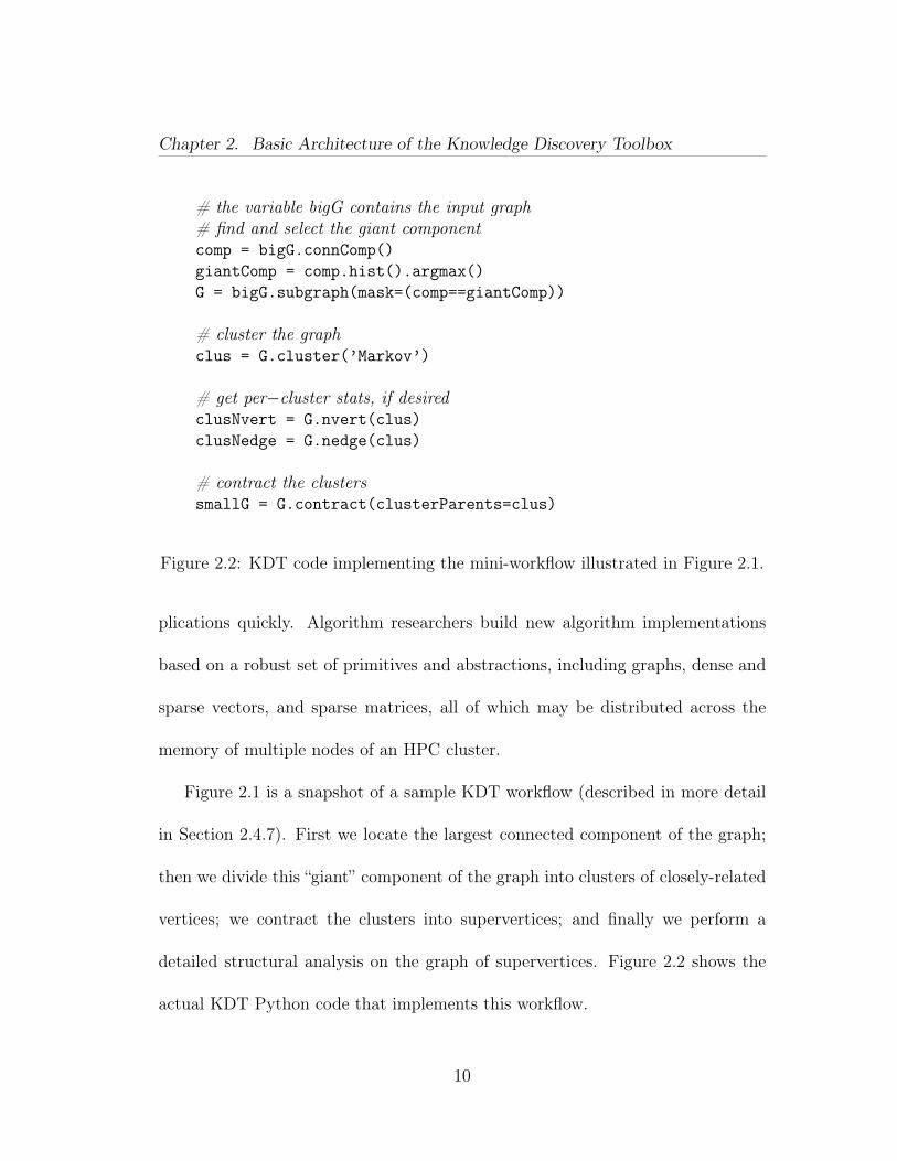
Chapter 2. Basic Architecture of the Knowledge Discovery Toolbox
# the variable bigG contains the input graph# find and select the giant componentcomp = bigG.connComp()giantComp = comp.hist().argmax()G = bigG.subgraph(mask=(comp==giantComp))
# cluster the graphclus = G.cluster(’Markov’)
# get per−cluster stats, if desiredclusNvert = G.nvert(clus)clusNedge = G.nedge(clus)
# contract the clusterssmallG = G.contract(clusterParents=clus)
Figure 2.2: KDT code implementing the mini-workflow illustrated in Figure 2.1.
plications quickly. Algorithm researchers build new algorithm implementations
based on a robust set of primitives and abstractions, including graphs, dense and
sparse vectors, and sparse matrices, all of which may be distributed across the
memory of multiple nodes of an HPC cluster.
Figure 2.1 is a snapshot of a sample KDT workflow (described in more detail
in Section 2.4.7). First we locate the largest connected component of the graph;
then we divide this “giant” component of the graph into clusters of closely-related
vertices; we contract the clusters into supervertices; and finally we perform a
detailed structural analysis on the graph of supervertices. Figure 2.2 shows the
actual KDT Python code that implements this workflow.
10
Chapter 2. Basic Architecture of the Knowledge Discovery Toolbox
KDT
Data filtering
technologies
Build input graph
Analyze graph
Cull relevant data
Interpret results
Graph viz
engine
3 2 1 4
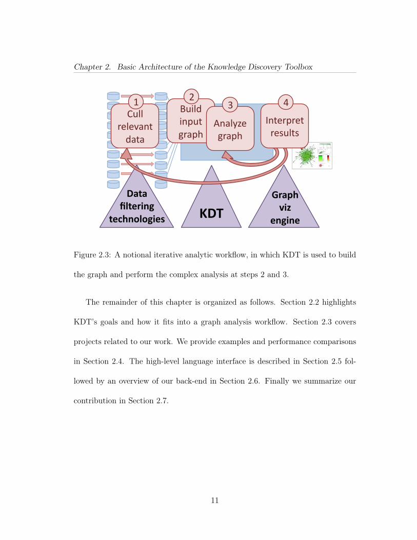
Figure 2.3: A notional iterative analytic workflow, in which KDT is used to build
the graph and perform the complex analysis at steps 2 and 3.
The remainder of this chapter is organized as follows. Section 2.2 highlights
KDT’s goals and how it fits into a graph analysis workflow. Section 2.3 covers
projects related to our work. We provide examples and performance comparisons
in Section 2.4. The high-level language interface is described in Section 2.5 fol-
lowed by an overview of our back-end in Section 2.6. Finally we summarize our
contribution in Section 2.7.
11
Chapter 2. Basic Architecture of the Knowledge Discovery Toolbox
2.2 Architecture and Context
A repeated theme in discussions with likely user communities for complex
graph analysis is that the domain expert analyzing a graph often does not know
in advance exactly what questions he or she wants to ask of the data. Therefore,
support for interactive trial-and-error use is essential.
Figure 2.3 sketches a high-level analytical workflow that consists of (1) culling
possibly relevant data from a data store (possibly disk files, a distributed database,
or streaming data) and cleansing it; (2) constructing the graph; (3) performing
complex analysis of the graph; and (4) interpreting key portions or subgraphs of
the result graph. Based on the results of step 4, the user may finish, loop back to
step 3 to analyze the same data differently, or loop back to step 1 to select other
data to analyze.
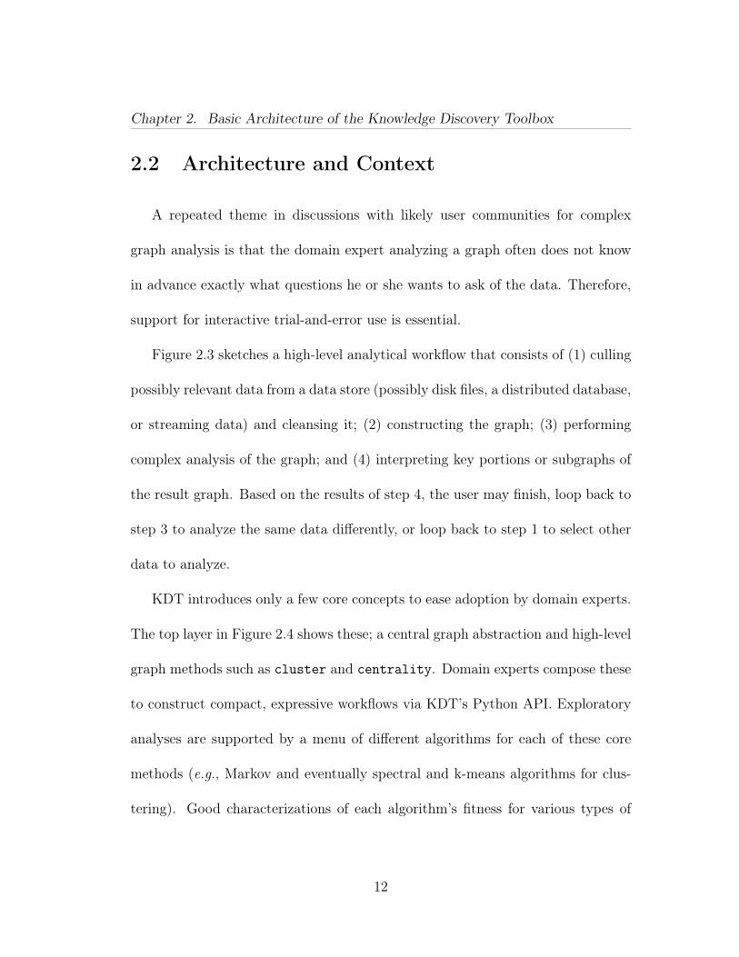
KDT introduces only a few core concepts to ease adoption by domain experts.
The top layer in Figure 2.4 shows these; a central graph abstraction and high-level
graph methods such as cluster and centrality. Domain experts compose these
to construct compact, expressive workflows via KDT’s Python API. Exploratory
analyses are supported by a menu of different algorithms for each of these core
methods (e.g., Markov and eventually spectral and k-means algorithms for clus-
tering). Good characterizations of each algorithm’s fitness for various types of
12
Chapter 2. Basic Architecture of the Knowledge Discovery Toolbox
Ranking pageRank
centrality(‘approxBC’)
DiGraph HyGraph
Building blocks
Clustering cluster(‘Markov’)
contract
Vec
Semiring methods (SpMV, SpGEMM)
Complex methods
Sparse-‐matrix classes/methods (e.g., Apply, EWiseApply, Reduce)
Underlying infrastructure (Combinatorial BLAS)
Mat • bfsTree,neighbor • degree,subgraph • load,UFget • +, -‐, sum, scale • generators
• toDiGraph • load, Ufget • bfsTree • degree
• SpMV • SpGEMM • load, save, eye • reduce, scale • EWiseApply, []
• max, norm,sort • abs, any, ceil • range, ones • EWiseApply,[]
other/future connComp triangles
Figure 2.4: The architecture of Knowledge Discovery Toolbox. The top-layer
methods are primarily used by domain experts, and include centrality and
cluster for semantic graphs. The middle-layer methods are primarily used by
graph-algorithm developers to implement the top-layer methods. KDT is layered
on top of Combinatorial BLAS.
very large data are rare and so most target users will not know in advance which
algorithms will work well for their data. We expect the set of high-level methods
to evolve over time.
The high-level methods are supported by a small number of carefully chosen
building blocks. KDT is targeted to analyze large graphs for which parallel execu-
13
Chapter 2. Basic Architecture of the Knowledge Discovery Toolbox
tion in distributed memory is vital, so its primitives are tailored to work on entire
collections of vertices and edges. As the middle layer in Figure 2.4 illustrates,
these include directed graphs (DiGraph), hypergraphs (HyGraph), and matrices
and vectors (Mat, Vec). The building blocks support lower-level graph and sparse
matrix methods (for example, degree, bfsTree, and SpGEMM). This is the level at
which the graph algorithm developer or researcher programs KDT.
Our current computational engine is Combinatorial BLAS [24] (shortened to
CombBLAS), which gives excellent and highly scalable performance on distributed-
memory HPC clusters. It forms the bottom layer of our software stack.
Knowledge discovery is a new and rapidly changing field, so KDT’s architec-
ture fosters extensibility. For example, a new clustering algorithm can easily be
added to the cluster routine, reusing most of the existing interface. This makes it
easy for the user to adopt a new algorithm merely by changing the algorithm ar-
gument. Since KDT is open-source (available at http://kdt.sourceforge.net),
algorithm researchers can look at existing methods to understand implementation
details, to tweak algorithms for their specific needs, or to guide the development
of new methods.
14
Chapter 2. Basic Architecture of the Knowledge Discovery Toolbox
2.3 Related Work
KDT combines a high-level language environment, to make both domain users
and algorithm developers more productive, with a high-performance computa-
tional engine to allow scaling to massive graphs. Several other research systems
provide some of these features, though we believe that KDT is the first to integrate
them all.
Titan [103] is a component-based pipeline architecture for ingestion, process-
ing, and visualization of informatics data that can be coupled to various high-
performance computing platforms. Pegasus [55] is a graph-analysis package that
uses MapReduce [31] in a distributed-computing setting. Pegasus uses a general-
ized sparse matrix-vector multiplication primitive called GIM-V, much like KDT’s
SpMV, to express vertex-centered computations that combine data from neighbor-
ing edges and vertices. This style of programming is called “think like a vertex”
in Pregel [78], a distributed-computing graph API. In traditional scientific com-
puting terminology, these are all BLAS-2 level operations; neither Pegasus nor
Pregel currently includes KDT’s BLAS-3 level SpGEMM “friends of friends” primi-
tive. BLAS-3 operations are higher level primitives that enable more optimizations
and generally deliver superior performance. Pregel’s C++ API targets efficiency-
15
Chapter 2. Basic Architecture of the Knowledge Discovery Toolbox
layer programmers, a different audience than the non-parallel-computing-expert
domain experts (scientists and analysts) targeted by KDT.
Libraries for high-performance computation on large-scale graphs include the
Parallel Boost Graph Library [50], the Combinatorial BLAS [24], and the Multi-
threaded Graph Library [14]. All of these libraries target efficiency-layer program-
mers, with lower-level language bindings and more explicit control over primitives.
GraphLab [69] is an example of an application-specific system for parallel
graph computing, in the domain of machine learning algorithms. Unlike KDT,
GraphLab runs only on shared-memory architectures.
2.4 Examples of use
In this section, we describe experiences using the KDT abstractions as graph-
analytic researchers, implementing complex algorithms intended as part of KDT
itself (breadth-first search, betweenness centrality, PageRank, Gaussian belief
propagation, and Markov clustering), and as graph-analytic users, implementing
a mini-workflow.
16
Chapter 2. Basic Architecture of the Knowledge Discovery Toolbox
1 1
1 1 1 1 1
1 1 1 1
1 7
7 7 7
7 7 7
3 4 5
4
4
5
4
7 7 7 5
1 1
1 1 1 1 1
1 1 1 1
1
fin fout G parents
×
×
=
=
root
1st Fron6er
2nd Fron6er fi = i
1 2
3
4 7
6
5
new
1 2
3
4 7
6
5
new
old
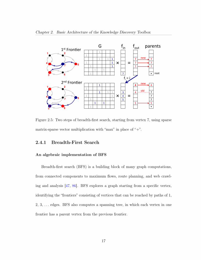
Figure 2.5: Two steps of breadth-first search, starting from vertex 7, using sparse
matrix-sparse vector multiplication with “max” in place of “+”.
2.4.1 Breadth-First Search
An algebraic implementation of BFS
Breadth-first search (BFS) is a building block of many graph computations,
from connected components to maximum flows, route planning, and web crawl-
ing and analysis [47, 86]. BFS explores a graph starting from a specific vertex,
identifying the “frontiers” consisting of vertices that can be reached by paths of 1,
2, 3, . . . edges. BFS also computes a spanning tree, in which each vertex in one
frontier has a parent vertex from the previous frontier.
17
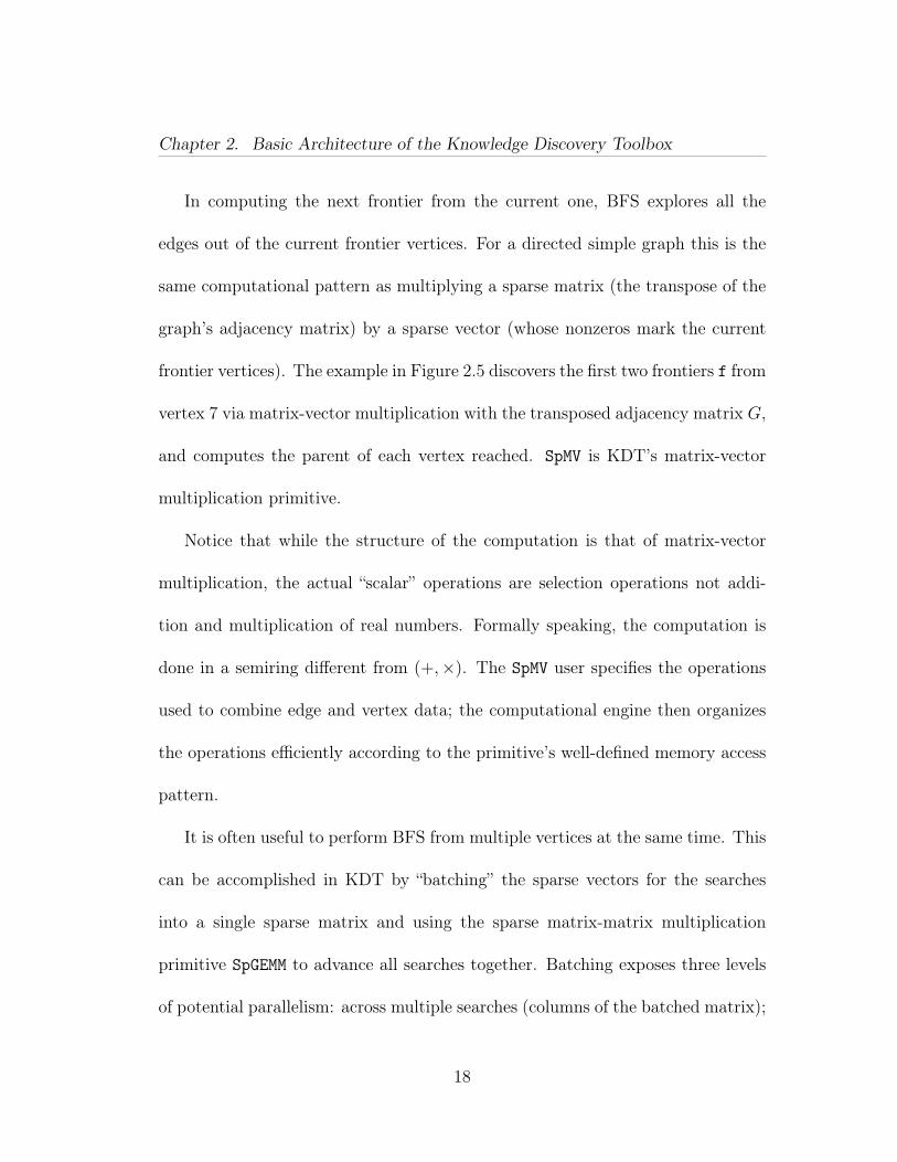
Chapter 2. Basic Architecture of the Knowledge Discovery Toolbox
In computing the next frontier from the current one, BFS explores all the
edges out of the current frontier vertices. For a directed simple graph this is the
same computational pattern as multiplying a sparse matrix (the transpose of the
graph’s adjacency matrix) by a sparse vector (whose nonzeros mark the current
frontier vertices). The example in Figure 2.5 discovers the first two frontiers f from
vertex 7 via matrix-vector multiplication with the transposed adjacency matrix G,
and computes the parent of each vertex reached. SpMV is KDT’s matrix-vector
multiplication primitive.
Notice that while the structure of the computation is that of matrix-vector
multiplication, the actual “scalar” operations are selection operations not addi-
tion and multiplication of real numbers. Formally speaking, the computation is
done in a semiring different from (+,×). The SpMV user specifies the operations
used to combine edge and vertex data; the computational engine then organizes
the operations efficiently according to the primitive’s well-defined memory access
pattern.
It is often useful to perform BFS from multiple vertices at the same time. This
can be accomplished in KDT by “batching” the sparse vectors for the searches
into a single sparse matrix and using the sparse matrix-matrix multiplication
primitive SpGEMM to advance all searches together. Batching exposes three levels
of potential parallelism: across multiple searches (columns of the batched matrix);
18
Chapter 2. Basic Architecture of the Knowledge Discovery Toolbox
across multiple frontier vertices in each search (rows of the batched matrix or
columns of the transposed adjacency matrix); and across multiple edges out of a
single high-degree frontier vertex (rows of the transposed adjacency matrix). The
Combinatorial BLAS SpGEMM implementation exploits all three levels of parallelism
when appropriate.
The Graph500 Benchmark
The intent of the Graph500 benchmark [49] is to rank computer systems by
their capability for basic graph analysis just as the Top500 list [83] ranks systems
by capability for floating-point numerical computation. The benchmark measures
the speed of a computer performing a BFS on a specified input graph in traversed
edges per second (TEPS). The benchmark graph is a synthetic undirected graph
with vertex degrees approximating a power law, generated by the RMAT [66]
algorithm. The size of the benchmark graph is measured by its scale, the base-2
logarithm of the number of vertices; the number of edges is about 16 times the
number of vertices. The RMAT generation parameters are a = 0.59, b = c =
0.19, d = 0.05, resulting in graphs with highly skewed degree distributions and
a low diameter. We symmetrize the input to model undirected graphs, but we
only count the edges traversed in the original graph for TEPS calculation, despite
visiting the symmetric edges as well.
19
Chapter 2. Basic Architecture of the Knowledge Discovery Toolbox
We have implemented the Graph500 code in KDT, including the parallel graph
generator, the BFS itself, and the validation required by the benchmark specifi-
cation. Per the spec, the validation consists of a set of consistency checks of the
BFS spanning tree. The checks verify that the tree spans an entire connected
component of the graph, that the tree has no cycles, that tree edges connect ver-
tices whose BFS levels differ by exactly one, and that every edge in the connected
component has endpoints whose BFS levels differ by at most one. All of these
checks are simple to perform with KDT’s elementwise operators and SpMV.
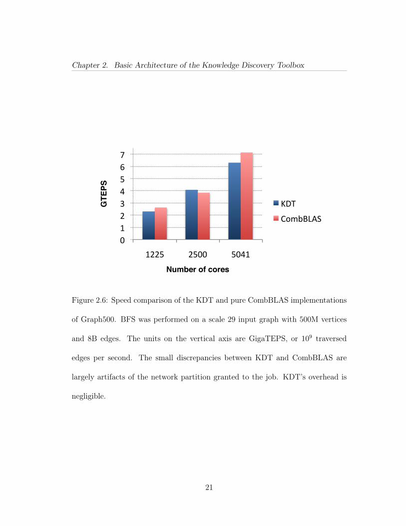
Figure 2.6 gives Graph500 TEPS scores for both KDT and for a custom
C++ code that calls the Combinatorial BLAS engine directly. Both runs are per-
formed on the Hopper machine at NERSC, which is a Cray XE6. Each XE6
node has two twelve-core 2.1 Ghz AMD Opteron processors, connected to the
Cray Gemini interconnect. The C++ portions of KDT are compiled with GNU
C++ compiler v4.5, and the Python interpreter is version 2.7. We utilized all the
cores in each node during the experiments. In other words, an experiment on p
cores ran on dp/24e nodes. The two-dimensional parallel BFS algorithm used by
Combinatorial BLAS is detailed elsewhere [26].
We see that KDT introduces negligible overhead; its performance is identical to
CombBLAS, up to small discrepancies that are artifacts of the network partition
granted to the job. The absolute TEPS scores are competitive; the purpose-built
20
Chapter 2. Basic Architecture of the Knowledge Discovery Toolbox
0 1 2 3 4 5 6 7
1225 2500 5041
GTE
PS!
Number of cores!
KDT
CombBLAS
Figure 2.6: Speed comparison of the KDT and pure CombBLAS implementations
of Graph500. BFS was performed on a scale 29 input graph with 500M vertices
and 8B edges. The units on the vertical axis are GigaTEPS, or 109 traversed
edges per second. The small discrepancies between KDT and CombBLAS are
largely artifacts of the network partition granted to the job. KDT’s overhead is
negligible.
21
Chapter 2. Basic Architecture of the Knowledge Discovery Toolbox
application used for the official June 2011 Graph500 submission for NERSC’s
Hopper has a TEPS rating about 4 times higher (using 8 times more cores), while
KDT is reusable for a variety of graph-analytic workflows.
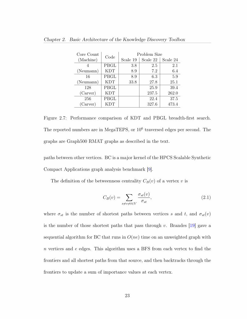
We compare KDT’s BFS against a PBGL BFS implementation in two envi-
ronments. Neumann is a shared memory machine composed of eight quad-core
AMD Opteron 8378 processors. It used version 1.47 of the Boost library, Python
2.4.3, and both PBGL and KDT were compiled with GCC 4.1.2. Carver is an
IBM iDataPlex system with 400 compute nodes, each node having two quad-core
Intel Nehalem processors. Carver used version 1.45 of the Boost library, Python
2.7.1, and both codes were compiled with Intel C++ compiler version 11.1. The
test data consists of scale 19 to 24 RMAT graphs. We did not use Hopper in these
experiments as PBGL failed to compile on the Cray platform.
The comparison results are presented in Figure 2.7. We observe that on this
example KDT is significantly faster than PBGL both in shared and distributed
memory, and that in distributed memory KDT exhibits robust scaling with in-
creasing processor count.
2.4.2 Betweenness Centrality
Betweenness centrality (BC) [39] is a widely accepted importance measure for
the vertices of a graph, where a vertex is “important” if it lies on many shortest
22
Chapter 2. Basic Architecture of the Knowledge Discovery Toolbox
Core Count Code Problem Size(Machine) Scale 19 Scale 22 Scale 24
4 PBGL 3.8 2.5 2.1(Neumann) KDT 8.9 7.2 6.4
16 PBGL 8.9 6.3 5.9(Neumann) KDT 33.8 27.8 25.1
128 PBGL 25.9 39.4(Carver) KDT 237.5 262.0
256 PBGL 22.4 37.5(Carver) KDT 327.6 473.4
Figure 2.7: Performance comparison of KDT and PBGL breadth-first search.
The reported numbers are in MegaTEPS, or 106 traversed edges per second. The
graphs are Graph500 RMAT graphs as described in the text.
paths between other vertices. BC is a major kernel of the HPCS Scalable Synthetic
Compact Applications graph analysis benchmark [9].
The definition of the betweenness centrality CB(v) of a vertex v is
CB(v) =∑
s 6=v 6=t∈V
σst(v)
σst, (2.1)
where σst is the number of shortest paths between vertices s and t, and σst(v)
is the number of those shortest paths that pass through v. Brandes [19] gave a
sequential algorithm for BC that runs in O(ne) time on an unweighted graph with
n vertices and e edges. This algorithm uses a BFS from each vertex to find the
frontiers and all shortest paths from that source, and then backtracks through the
frontiers to update a sum of importance values at each vertex.
23
Chapter 2. Basic Architecture of the Knowledge Discovery Toolbox
The quadratic running time of BC is prohibitive for large graphs, so one typi-
cally computes an approximate BC by performing BFS only from a sampled subset
of vertices [10].
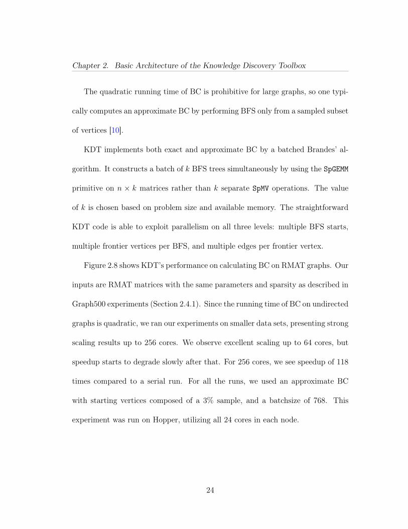
KDT implements both exact and approximate BC by a batched Brandes’ al-
gorithm. It constructs a batch of k BFS trees simultaneously by using the SpGEMM
primitive on n × k matrices rather than k separate SpMV operations. The value
of k is chosen based on problem size and available memory. The straightforward
KDT code is able to exploit parallelism on all three levels: multiple BFS starts,
multiple frontier vertices per BFS, and multiple edges per frontier vertex.
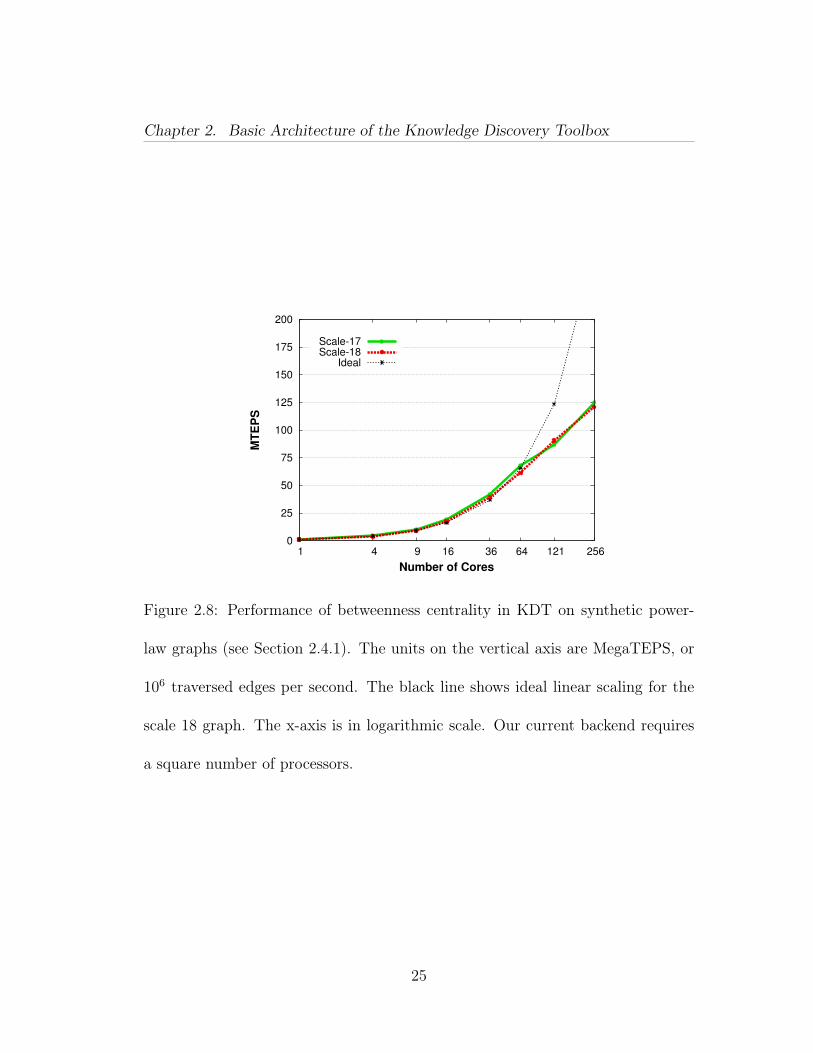
Figure 2.8 shows KDT’s performance on calculating BC on RMAT graphs. Our
inputs are RMAT matrices with the same parameters and sparsity as described in
Graph500 experiments (Section 2.4.1). Since the running time of BC on undirected
graphs is quadratic, we ran our experiments on smaller data sets, presenting strong
scaling results up to 256 cores. We observe excellent scaling up to 64 cores, but
speedup starts to degrade slowly after that. For 256 cores, we see speedup of 118
times compared to a serial run. For all the runs, we used an approximate BC
with starting vertices composed of a 3% sample, and a batchsize of 768. This
experiment was run on Hopper, utilizing all 24 cores in each node.
24
Chapter 2. Basic Architecture of the Knowledge Discovery Toolbox
0
25
50
75
100
125
150
175
200
1 4 9 16 36 64 121 256
MT
EP
S
Number of Cores
Scale-17
Scale-18
Ideal
Figure 2.8: Performance of betweenness centrality in KDT on synthetic power-
law graphs (see Section 2.4.1). The units on the vertical axis are MegaTEPS, or
106 traversed edges per second. The black line shows ideal linear scaling for the
scale 18 graph. The x-axis is in logarithmic scale. Our current backend requires
a square number of processors.
25
Chapter 2. Basic Architecture of the Knowledge Discovery Toolbox
2.4.3 PageRank
PageRank [88] computes vertex relevance by modeling the actions of a “random
surfer”. At each vertex (i.e., web page) the surfer either traverses a randomly-
selected outbound edge (i.e., link) of the current vertex, excluding self loops, or the
surfer jumps to a randomly-selected vertex in the graph. The probability that the
surfer chooses to traverse an outbound edge is controlled by the damping factor,
d. A typical damping factor in practice is 0.85. The output of the algorithm is
the probability of finding the surfer visiting a particular vertex at any moment,
which is the stationary distribution of the Markov chain that describes the surfer’s
moves.
KDT computes PageRank by iterating the Markov chain, beginning by ini-
tializing vertex probabilities P0(v) = 1/n for all vertices v in the graph, where n
is the number of vertices and the subscript denotes the iteration number. The
algorithm updates the probabilities iteratively by computing
Pk+1(v) =1− dn
+ d∑
u∈Adj−(v)
Pk(u)
|Adj+(u)|, (2.2)
where Adj−(u) and Adj+(u) are the sets of inbound and outbound vertices adjacent
to u. Vertices with no outbound edges are treated as if they link to all vertices.
After removing self loops from the graph, KDT evaluates (2.2) simultaneously
for all vertices using the SpMV primitive. The iteration process stops when the
26
Chapter 2. Basic Architecture of the Knowledge Discovery Toolbox
1-norm of the difference between consecutive iterates drops below a default or, if
supplied, user-defined stopping threshold ε.
We compare the PageRank implementations which ship with KDT and Pega-
sus in Figure 2.9. The dataset is composed of scale 19 and 21 directed RMAT
graphs with isolated vertices removed. The scale 19 graph contains 335K ver-
tices and 15.5M edges, the scale 21 graph contains 1.25M vertices and 63.5M
edges and the convergence criteria is ε = 10−7. The test machine is Neumann
(a 32-core shared memory machine, same hardware and software configuration
as in Section 2.4.1). We used Pegasus 2.0 running on Hadoop 0.20.204 and Sun
JVM 1.6.0_13. We directly compare KDT core counts with maximum MapRe-
duce task counts despite this giving Pegasus an advantage (each task typically
shows between 110%-190% CPU utilization). We also observed that mounting
the Hadoop Distributed Filesystem in a ramdisk provided Pegasus with a speed
boost on the order of 30%. Despite these advantages we still see that KDT is two
orders of magnitude faster.
Both implementations are fundamentally based on an SpMV operation, but
Pegasus performs it via a MapReduce framework. MapReduce allows Pegasus to
be able to handle huge graphs that do not fit in RAM. However, the penalty for
this ability is the need to continually touch disk for every intermediate operation,
parsing and writing intermediate data from/to strings, global sorts, and spawning
27
Chapter 2. Basic Architecture of the Knowledge Discovery Toolbox
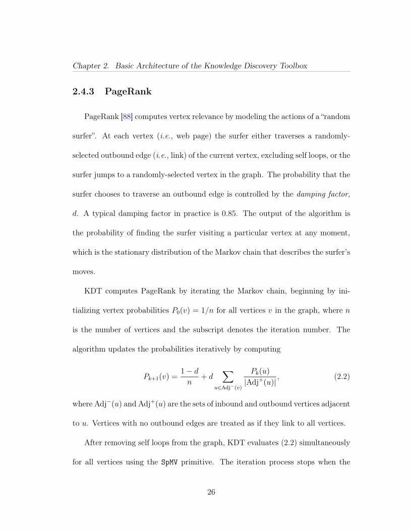
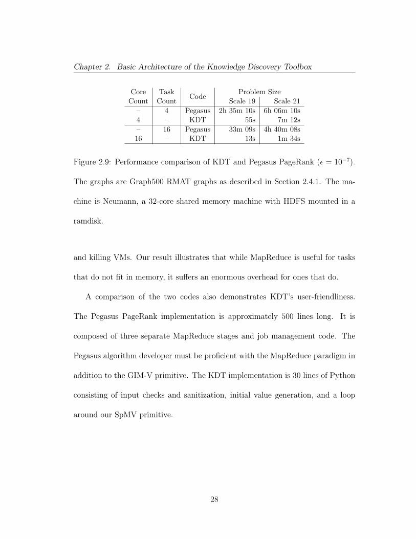
Core Task Code Problem SizeCount Count Scale 19 Scale 21
– 4 Pegasus 2h 35m 10s 6h 06m 10s4 – KDT 55s 7m 12s– 16 Pegasus 33m 09s 4h 40m 08s16 – KDT 13s 1m 34s
Figure 2.9: Performance comparison of KDT and Pegasus PageRank (ε = 10−7).
The graphs are Graph500 RMAT graphs as described in Section 2.4.1. The ma-
chine is Neumann, a 32-core shared memory machine with HDFS mounted in a
ramdisk.
and killing VMs. Our result illustrates that while MapReduce is useful for tasks
that do not fit in memory, it suffers an enormous overhead for ones that do.
A comparison of the two codes also demonstrates KDT’s user-friendliness.
The Pegasus PageRank implementation is approximately 500 lines long. It is
composed of three separate MapReduce stages and job management code. The
Pegasus algorithm developer must be proficient with the MapReduce paradigm in
addition to the GIM-V primitive. The KDT implementation is 30 lines of Python
consisting of input checks and sanitization, initial value generation, and a loop
around our SpMV primitive.
28
Chapter 2. Basic Architecture of the Knowledge Discovery Toolbox
2.4.4 Belief Propagation
Belief Propagation (BP) is a so-called “message passing” algorithm for per-
forming inference on graphical models such as Bayesian networks [113]. Graphical
models are used extensively in machine learning, where each random variable is
represented as a vertex and the conditional dependencies among random variables
are represented as edges. BP calculates the approximate marginal distribution for
each unobserved vertex, conditional on any observed vertices.
Gaussian Belief Propagation (GaBP) is a version of the BP algorithm in which
the underlying distributions are modeled as Gaussian [15]. GaBP can be used to
iteratively solve symmetric positive definite systems of linear equations Ax = b,
and thus is a potential candidate for solving linear systems that arise within KDT.
Although BP is applicable to much more general settings (and is not necessarily
the method of choice for solving a linear equation system), GaBP is often used as
a performance benchmark for BP implementations.
We implemented GaBP in KDT and used it to solve a steady-state thermal
problem on an unstructured mesh. The algorithm converged after 11 iterations
on the Schmid/thermal2 problem that has 1.2 million vertices and 8.5 million
edges [29].
We demonstrate strong scaling using steady-state 2D heat dissipation problems
in Figure 2.10. The k × k 2D grids yield graphs with k2 vertices and 5k2 edges.
29
Chapter 2. Basic Architecture of the Knowledge Discovery Toolbox
0
1000
2000
3000
4000
5000
6000
4 16 36 64 121 256 529 0
10
20
30
40
50
60
Seco
nd
s
Sp
eed
up
Number of Cores
Time (s)Speedup
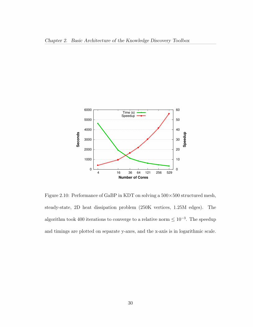
Figure 2.10: Performance of GaBP in KDT on solving a 500×500 structured mesh,
steady-state, 2D heat dissipation problem (250K vertices, 1.25M edges). The
algorithm took 400 iterations to converge to a relative norm ≤ 10−3. The speedup
and timings are plotted on separate y-axes, and the x-axis is in logarithmic scale.
30
Chapter 2. Basic Architecture of the Knowledge Discovery Toolbox
We observed linear scaling with increasing problem size and were able to solve
a k = 4000 problem in 31 minutes on 256 cores. Parallel scaling is sub-linear
because GaBP is an iterative algorithm with low arithmetic intensity which makes
it bandwidth (to RAM) bound. The above experiments were run on Hopper, but
we observed similar scaling on the Neumann shared memory machine.
We compared our GaBP implementation with GraphLab’s GaBP on our shared
memory system. The problem set was composed of structured and unstructured
meshes ranging from hundreds of edges to millions. KDT’s time to solution com-
pared favorably with GraphLab on problems with more than 10,000 edges.
2.4.5 Markov Clustering
Markov Clustering (MCL) [105] is used in computational biology to discover
the members of protein complexes [35, 20], in linguistics to separate the related
word clusters of homonyms [34], and to find circles of trust in social network
graphs [89, 82]. MCL finds clusters by postulating that a random walk that visits
a dense cluster will probably visit many of its vertices before leaving.
The basic algorithm operates on the graph’s adjacency matrix. It iterates a
sequence of steps called expansion, inflation, normalization and pruning. The ex-
pansion step discovers friends-of-friends by raising the matrix to a power (typically
2). Inflation separates low- and high-weight edges by raising the individual matrix
31
Chapter 2. Basic Architecture of the Knowledge Discovery Toolbox
elements to a power which can vary from about 2 to 20, higher values producing
finer clusters. This has the effect of both strengthening flow inside clusters and
weakening it between clusters. The matrix is scaled to be column-stochastic by
a normalization step. The pruning step is one key to MCL’s efficiency because it
preserves sparsity. Our implementation prunes elements which fall below a thresh-
old though other pruning strategies are possible. These steps are repeated until
convergence, then the clusters are identified. The standard, and KDT’s default,
method is to identify the connected components of the pruned graph as clusters.
The KDT Markov clustering method provides sensible defaults for all parameters
and options, but allows the user to override them if desired.
2.4.6 Peer-Pressure Clustering
Peer Pressure is a clustering algorithm based on the observation that for a
given graph clustering the cluster assignment of a vertex will be the same as that
of most of its neighbors.
The algorithm starts with a base case of an initial cluster assignment, such
as each vertex being in its own cluster. Each iteration performs an election at
each vertex to select which cluster that vertex should belong to at the end of
the iteration. The votes are the cluster assignments of its neighbors. Ties are
settled by selecting the lowest cluster ID to maintain determinism, but can be
32
Chapter 2. Basic Architecture of the Knowledge Discovery Toolbox
settled arbitrarily. The algorithm converges when two consecutive iterations have
a (tunably) small difference between them.
This algorithm can take up to O(# of vertices) iterations in pathological cases,
however it typically converges in a small number of iterations (on the order of five
to ten) on well-clustered graphs.
This algorithm is also known by the name Label Propagation [92] in the physics
literature. Boldi et. al. [16] extend that work with Layered Label Propagation
which accepts a parameter γ which selects between large relatively sparse clusters
and small relatively dense clusters.
RDF/SPARQL Implementation
Chapter ?? is about our Peer Pressure implementation in RDF/SPARQL for
YarcData’s uRiKA appliance.
2.4.7 Mini-workflow Example
End-to-end graph analysis workflows vary greatly between domains, between
problems, and likely even between individual analysts; we do not attempt to
describe them here. However, we can identify some smaller mini-workflows as
being close enough to real workflows to serve as examples. One mini-workflow,
33
Chapter 2. Basic Architecture of the Knowledge Discovery Toolbox
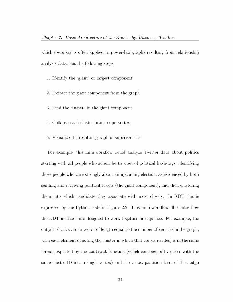
which users say is often applied to power-law graphs resulting from relationship
analysis data, has the following steps:
1. Identify the “giant” or largest component
2. Extract the giant component from the graph
3. Find the clusters in the giant component
4. Collapse each cluster into a supervertex
5. Visualize the resulting graph of supervertices
For example, this mini-workflow could analyze Twitter data about politics
starting with all people who subscribe to a set of political hash-tags, identifying
those people who care strongly about an upcoming election, as evidenced by both
sending and receiving political tweets (the giant component), and then clustering
them into which candidate they associate with most closely. In KDT this is
expressed by the Python code in Figure 2.2. This mini-workflow illustrates how
the KDT methods are designed to work together in sequence. For example, the
output of cluster (a vector of length equal to the number of vertices in the graph,
with each element denoting the cluster in which that vertex resides) is in the same
format expected by the contract function (which contracts all vertices with the
same cluster-ID into a single vertex) and the vertex-partition form of the nedge
34
Chapter 2. Basic Architecture of the Knowledge Discovery Toolbox
function. The output of this example workflow for a tiny input graph is illustrated
in Figure 2.1.
2.5 High Level Language Interface
2.5.1 High Productivity for Graph Analysis
KDT targets a demanding environment – domain experts exploring novel very
large graphs with hard-to-specify goals. Today this requires knowledge in so many
domains that only the most talented, cross-disciplinary, and well-funded groups
succeed. KDT aims not only to enable these (non-graph-expert) domain experts
to analyze very large graphs quickly but also to accelerate the work of graph-
algorithm researchers developing the next generation of algorithms attacking the
inherent combinatorial wall of graph analysis.
KDT delivers high productivity to domain experts by limiting the number of
new concepts and by providing powerful abstractions for both data and meth-
ods. For instance, the DiGraph class implements directed graphs for distributed
memory, hiding the details of how the directed graph is represented in distributed
memory. Similarly, KDT users use the cluster method to cluster a graph’s
vertices by an (initially brief) menu of algorithms. Detailed algorithm-specific
options such as the expansion and inflation factors for Markov clustering default
35
Chapter 2. Basic Architecture of the Knowledge Discovery Toolbox
to appropriate values for the typical user but enable more knowledgeable users to
exercise more control if needed. Those wanting even more control are provided
with methods that are too detailed for many domain experts. These include access
to well optimized linear algebraic methods and additional graph methods such as
bfsTree and normalizeEdgeWeights
Our experience implementing the primary methods of KDT may illustrate the
productivity of this approach. One of us implemented exact betweenness cen-
trality in Python using serial SciPy. Moving that code to run in a distributed
parallel manner with KDT required changing the initial definitions of (e.g. vari-
able arrays), but much of the core code (e.g. multiplying and adding intermediate
matrices) did not change. The changes took only 11 hours of programming time
for the BC routine itself. The resulting code runs correctly and scales effec-
tively to hundreds of cores. Similarly, after initial explorations to understand the
Markov Clustering algorithm and KDT well, an undergraduate student produced
our Markov Clustering routine in only six hours.
2.5.2 Organization of the Fundamental Classes
KDT’s productivity benefits extend beyond simply providing an opaque set of
built-in graph algorithms. The provided set of algorithms also serve as guides for
36
Chapter 2. Basic Architecture of the Knowledge Discovery Toolbox
users who want to implement their own graph algorithms based on our extensible
primitives.
As Figure 2.4 illustrates, the kdt Python module exposes two types of classes:
graph objects and their supporting linear algebraic objects. It includes classes
representing directed graphs (DiGraph), hypergraphs (HyGraph), as well as sparse
matrices (Mat) and sparse and dense vectors (Vec). Computation is performed
using a set of pre-defined patterns:
• Matrix-Matrix multiplication (SpGEMM), Matrix-Vector multiplication (SpMV)
• Element-wise (EWiseApply)
• Querying operations (Count, Reduce, Find)
• Indexing and Assignment (SubsRef, SpAsgn)
These operations are the key to KDT’s scalability. Each one is implemented for
parallel execution and accepts user-defined callbacks that act similarly to visitors.
The pre-defined access patterns allow considerable scalability and account for the
bulk of processing time. This allows KDT code to appear serial yet have parallel
semantics.
The sparse matrix and vector classes that support the graph classes are exposed
to allow complex matrix analysis techniques (e.g., spectral methods). Directed
graphs are represented using an n × n sparse adjacency matrix. Hypergraphs
37
Chapter 2. Basic Architecture of the Knowledge Discovery Toolbox
use an n ×m rectangular incidence matrix. Note that bipartite graphs can also
be represented with a hypergraph. A graph’s edge attributes are represented as
the matrix’s element values while vertex attributes are stored in vectors of length
matching the matrix dimension. KDT’s matrices and vectors can be of several
types including boolean for connectivity only, floating point, and custom objects.
User-defined callbacks can take several forms. KDT operations accept unary,
binary and n-ary operations, predicates, and semiring functions. Each one may
be a built-in function or a user-written Python callback or wrapped C routine for
speed.
Taken together, these building blocks and finished algorithms provide KDT
with a high degree of power and flexibility.
2.5.3 Semantic Graphs
Users found that the initial release of KDT lacked support for semantic graphs,
i.e. graphs whose vertices and edges have types. Semantic graphs are valuable
when data is of disparate types (e.g. link data about communication via email,
Twitter, and Facebook) and considering different types of data together delivers
better insight. The KDT semantic graph interface enables on the fly selection of
vertices and edges via user-defined callbacks. Computations are only performed
on selected vertices and edges. In some situations the graph is very large and the
38
Chapter 2. Basic Architecture of the Knowledge Discovery Toolbox
user wants to select most of the graph, in which case materializing the selected
graph is wasteful of memory; in other cases the user wants to select only a small
portion of the graph, in which case materializing the smaller graph may be more
efficient. The KDT semantic graph operations appear to be a dual for SQL’s
ability to push certain computations onto the database.
The subsequent KDT release (v0.2) defines the notion of a filter. A filter deter-
mines whether or not a particular vertex or edge is included in the computation.
Our filter design relies on three basic principles.
1. A user-defined predicate determines whether or not a vertex or edge exists
in the filtered graph.
2. Multiple user-defined predicates can be stacked and the filters they define
are applied in the order they are added to the graph. Thus, both users and
algorithm developers can use filters.
3. All graph operations respect the filter. This ensures that algorithms can be
written without taking filters into consideration at all, thus greatly easing
their design.
For example, assume that a graph contains link data about communication
between employees via email, Twitter, and Facebook, and that a user wants to
39
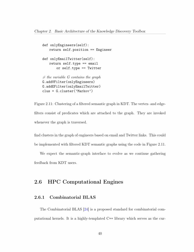
Chapter 2. Basic Architecture of the Knowledge Discovery Toolbox
def onlyEngineers(self):return self.position == Engineer
def onlyEmailTwitter(self):return self.type == email
or self.type == Twitter
# the variable G contains the graphG.addVFilter(onlyEngineers)G.addEFilter(onlyEmailTwitter)clus = G.cluster(’Markov’)
Figure 2.11: Clustering of a filtered semantic graph in KDT. The vertex- and edge-
filters consist of predicates which are attached to the graph. They are invoked
whenever the graph is traversed.
find clusters in the graph of engineers based on email and Twitter links. This could
be implemented with filtered KDT semantic graphs using the code in Figure 2.11.
We expect the semantic-graph interface to evolve as we continue gathering
feedback from KDT users.
2.6 HPC Computational Engines
2.6.1 Combinatorial BLAS
The Combinatorial BLAS [24] is a proposed standard for combinatorial com-
putational kernels. It is a highly-templated C++ library which serves as the cur-
40
Chapter 2. Basic Architecture of the Knowledge Discovery Toolbox
rent KDT backend. It offers a small set of linear algebraic kernels that can be
used as building blocks for the most common graph-analytic algorithms. Graph
abstractions can be built on top of its sparse matrices, taking advantage of its ex-
isting best practices for handling parallelism in sparse linear algebra. Its flexibility
comes from the arbitrary operations that it supports. The user, or in this case
the KDT implementor, specifies the add and multiply routines in matrix-matrix
and matrix-vector operations, or unary and binary functions for element-wise op-
erations. The main data structures are distributed sparse matrices and vectors,
which are distributed in a two-dimensional processor grid for scalability.
We use the publicly available MPI reference implementation of the Combi-
natorial BLAS as our computational engine. We extended its interface in order
to provide further capabilities, such as fully-distributed (to all the processors)
sparse vectors, sparse matrix-sparse vector multiplication, and routines akin to
MATLAB®’s sparse and find.
The primary KDT abstractions are different from Combinatorial BLAS ab-
stractions. CombBLAS exposes distributed-memory dense and sparse vectors and
sparse matrices and key operations on them, mostly linear algebra, required to
implement combinatorial problems. KDT exposes graph abstractions such as di-
rected graphs, and graph operations such as ranking vertices (e.g., betweenness
centrality or PageRank), clustering, and finding neighbors within k hops of a set
41
Chapter 2. Basic Architecture of the Knowledge Discovery Toolbox
of vertices; the underlying linear algebraic implementation is not immediately
visible. This shift in abstractions between the linear-algebra worldview and the
graph worldview is one of the primary contributions of KDT. It creates usability
for domain experts while retaining performance and customizability.
2.6.2 Evolution of KDT
The design of KDT intentionally separates its user-level language and interface
from its computational engine. This allows us to extend KDT easily along at least
two axes: an architectural axis, and a capability axis.
On the architectural axis, we intend KDT to map readily to computational
engines that provide the functionality of Combinatorial BLAS on different plat-
forms. We and our collaborators are currently working on two such engines: one
for manycore shared-address-space architectures, and one for more loosely coupled
distributed-computing cloud architectures. We are also contemplating engines
that will be able to use more specialized hardware, including GPUs, FPGAs, and
massively multithreaded architectures like Cray XMT [58].
On the capability axis, we are extending the set of algorithms and primitives
that underlie KDT in various ways. Numerical computational primitives such as
linear equation solvers and spectral analysis (computing eigenvalues, singular val-
ues, eigenvectors, etc.) are useful in many data analysis settings, and fit naturally
42
Chapter 2. Basic Architecture of the Knowledge Discovery Toolbox
into KDT’s parallel sparse matrix paradigm. We are also exploring some other
classes of graph primitives—for example, the visitor paradigm of the Boost Graph
Library and its relatives [100, 62, 50, 14].
In many cases, enhancing KDT’s capabilities means interfacing KDT to exist-
ing high-performance computational libraries; for example, an upcoming release
of KDT is planned to include the numerical PARPACK library [79, 63] in its com-
putational engine, and high-quality high-performance libraries for other numerical
computations exist [68, 52, 56].
One of our goals is to use the KDT API as a high-level interface to other
existing high-performance graph libraries (such as The MultiThreaded Graph Li-
brary [14] and Parallel Boost Graph Library [50]) and representations (such as
STINGER [8]). We expect that KDT’s high-level language interface will evolve
to permit different graph libraries to be used as back ends; we view the current
high-level Python specification as a starting point and we are actively soliciting
feedback from users and developers to help us guide its evolution.
2.7 Conclusion
The Knowledge Discovery Toolbox makes truly scalable graph analysis ac-
cessible in a high-level language to both domain experts and developers of graph
43
Chapter 2. Basic Architecture of the Knowledge Discovery Toolbox
analytics. The two key ingredients are a core set of graph abstractions (and accom-
panying Python API) providing flexibility and simplicity, and a high-performance
computational back end providing scalable performance for graphs in excess of
10 billion edges on HPC clusters. KDT version 0.2, released in 2012, implements
the core architecture, which are shown here to enable rapid development of both
highly performant graph-analytic workflows and the underlying graph-analytic op-
erations themselves. The performance of KDT approaches that of efficiency-level
applications while being reusable for a variety of graph-analytic workflows. In cur-
rent work, we are extending both KDT’s capabilities and the range of hardware
and software platforms on which it can be used.
44
Chapter 3
Attributed Semantic Graphs andFilters
This chapter is based on a paper published in ICASSP’12 [73].
3.1 Introduction
This chapter describes features of KDT that support graphs with attributes
on both edges and vertices (so-called semantic graphs), the design of KDT’s fil-
tering mechanism, and how these changes meet the criteria of customizability and
performance.
3.2 Semantic Graph Example
Consider the example of a social network where information is known about
cell-phone calls and text messages. To understand the patterns of communication
45
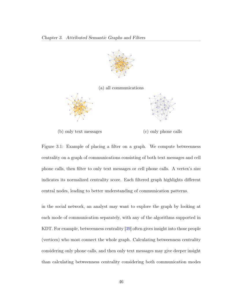
Chapter 3. Attributed Semantic Graphs and Filters
(a) all communications
(b) only text messages (c) only phone calls
Figure 3.1: Example of placing a filter on a graph. We compute betweenness
centrality on a graph of communications consisting of both text messages and cell
phone calls, then filter to only text messages or cell phone calls. A vertex’s size
indicates its normalized centrality score. Each filtered graph highlights different
central nodes, leading to better understanding of communication patterns.
in the social network, an analyst may want to explore the graph by looking at
each mode of communication separately, with any of the algorithms supported in
KDT. For example, betweenness centrality [39] often gives insight into those people
(vertices) who most connect the whole graph. Calculating betweenness centrality
considering only phone calls, and then only text messages may give deeper insight
than calculating betweenness centrality considering both communication modes
46
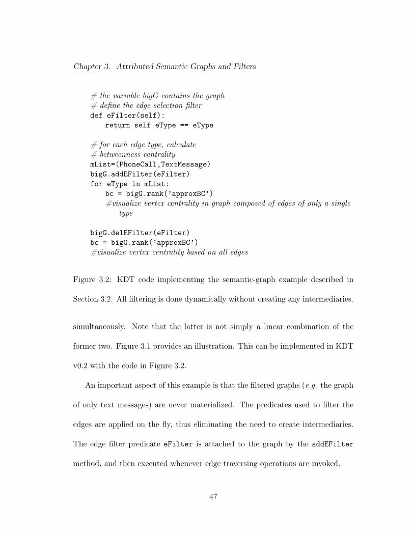
Chapter 3. Attributed Semantic Graphs and Filters
# the variable bigG contains the graph# define the edge selection filterdef eFilter(self):
return self.eType == eType
# for each edge type, calculate# betweenness centralitymList=(PhoneCall,TextMessage)bigG.addEFilter(eFilter)for eType in mList:
bc = bigG.rank(’approxBC’)#visualize vertex centrality in graph composed of edges of only a single
type
bigG.delEFilter(eFilter)bc = bigG.rank(’approxBC’)#visualize vertex centrality based on all edges
Figure 3.2: KDT code implementing the semantic-graph example described in
Section 3.2. All filtering is done dynamically without creating any intermediaries.
simultaneously. Note that the latter is not simply a linear combination of the
former two. Figure 3.1 provides an illustration. This can be implemented in KDT
v0.2 with the code in Figure 3.2.
An important aspect of this example is that the filtered graphs (e.g. the graph
of only text messages) are never materialized. The predicates used to filter the
edges are applied on the fly, thus eliminating the need to create intermediaries.
The edge filter predicate eFilter is attached to the graph by the addEFilter
method, and then executed whenever edge traversing operations are invoked.
47
Chapter 3. Attributed Semantic Graphs and Filters
This example has analogues in life sciences, where the different edges might
be protein-protein or protein-DNA interactions.
3.3 KDT Design
We build on our previous work on the Combinatorial BLAS (or CombBLAS
for short) [24] by utilizing it as our initial backend. The CombBLAS is a pro-
posed standard for combinatorial computational kernels. It is a highly-templated
C++ library. It offers a small set of linear algebraic kernels that can be used as
building blocks for the most common graph-analytic algorithms. Graph abstrac-
tions can be built on top of its sparse matrices, taking advantage of its existing
best practices for handling parallelism in sparse linear algebra. Its flexibility
comes from the arbitrary operations that it supports. The user, or in this case
the KDT implementor, specifies the add and multiply routines in matrix-matrix
and matrix-vector operations, or unary and binary functions for element-wise op-
erations. The main data structures are distributed sparse matrices and vectors,
which are distributed in a two-dimensional processor grid for scalability.
KDT transforms the linear algebra primitives into graph primitives. The
graph’s edges are collectively stored in a matrix, and vertex attributes are stored in
a vector. Sparse matrix-vector multiplication (SpMV) and sparse matrix-matrix
48
Chapter 3. Attributed Semantic Graphs and Filters
multiplication (SpGEMM) become KDT’s graph traversal primitives, where user
code in the add and multiply semiring routines defines the function of the traver-
sal. Element-wise operations become edge and vertex visitors. The main benefit
of this approach is that traditional graph frameworks are latency-bound whereas
linear algebra primitives are bandwidth bound. The latter is far more scalable.
Our first KDT release (described in Chapter 2) focused on providing key ab-
stractions on data structures and algorithms (e.g. digraphs, rank, cluster) and
the supporting infrastructure (vectors, matrices, Python bindings). Our goal was
to be able to deliver our world-class CombBLAS performance with conceptual
simplicity and user-friendly design. We did not focus on extending the graph
abstractions; instead we supported only floating-point attributes on both vertices
and edges.
The progression of capabilities of CombBLAS and KDT is illustrated in Figure
3.3.
49
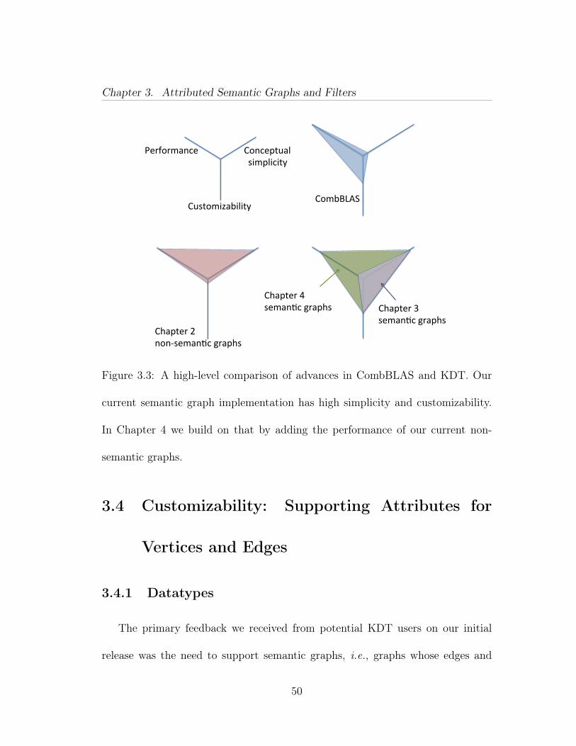
Chapter 3. Attributed Semantic Graphs and Filters
Chapter 3 seman-c graphs
Performance
Customizability
Conceptual simplicity
CombBLAS
Chapter 2 non-‐seman-c graphs
Chapter 4 seman-c graphs
Figure 3.3: A high-level comparison of advances in CombBLAS and KDT. Our
current semantic graph implementation has high simplicity and customizability.
In Chapter 4 we build on that by adding the performance of our current non-
semantic graphs.
3.4 Customizability: Supporting Attributes for
Vertices and Edges
3.4.1 Datatypes
The primary feedback we received from potential KDT users on our initial
release was the need to support semantic graphs, i.e., graphs whose edges and
50
Chapter 3. Attributed Semantic Graphs and Filters
vertices have attributes on them. The needed support consisted of two primary
changes to KDT: the ability to create graphs with edge objects more complex than
the single 64-bit data element of our first release (and similarly vectors with vertex
objects more complex than the 64-bit element), and the ability to customize KDT
operations to filter or compute on elements of the edge and vertex objects. These
changes must be made balanced with the conceptual simplicity and performance
requirements.
Our filter design relies on three basic principles.
1. A user-defined predicate determines whether or not a vertex or edge exists
in the filtered graph
2. Multiple user-defined predicates can be stacked and the filters they define
are applied in the order they are added to the graph. Thus, both users and
algorithm developers can use filters.
3. All graph operations respect the filter. This ensures that algorithms can be
written without taking filters into consideration at all, thus greatly easing
their design.
Two performance issues constrain the semantic-graph design in KDT. First,
KDT is targeted at complex graph analytics, which usually traverse the graph
more than simple analytics. These traversals are time-consuming, so to avoid
51
Chapter 3. Attributed Semantic Graphs and Filters
a catastrophic performance decrease when using semantic graphs in KDT, the
semantic-graph mechanisms must support computations that require only mini-
mally (and ideally no) more passes over the graph than the non-semantic case.
Second, because of the traversal-intensive nature of complex graph analytics and
the fact that in-memory operation is typically much faster than on-disk operation,
frugal memory use will enable much larger problems to be solved. Specifically,
when a user filters a graph to operate on only certain types of edges or vertices,
avoiding the materialization of the intermediate graph will typically be a large sav-
ing in memory consumption. KDT’s semantic-graph mechanisms strive to achieve
this.
Given that KDT interfaces are via Python, a natural target for customizable
data structures would be a fully general Python object. Unfortunately, Python
objects are so general that even their size might not remain constant during their
lifetime. KDT’s dependence on the Combinatorial BLAS, a C++ package, re-
quires a set of statically-typed and statically-sized objects known at compile time,
which does not lend itself to straightforward support of general run-time definable
Python objects. In practice, less-general structures targeted at semantic graphs
provide the support needed for many semantic-graph problems; e.g., STINGER
[8] has been proposed as a common graph data structure.
52
Chapter 3. Attributed Semantic Graphs and Filters
We are continually relaxing our requirements for what an attribute can be.
Our original implementation used simple 64-bit floating point scalar values as the
only supported attribute types.
KDT v0.2 provides two statically-defined object types, Obj1 and Obj2, which
are motivated by STINGER. Unlike STINGER, however, our users may modify
the object types, albeit in C++ at KDT compile time. Each object type, as well as
scalars, can be used for either edge or vertex attributes. With this data-structure
flexibility comes some additional user responsibility in defining how the elements
of the objects are used, i.e., how the load function will fill the members of the
object from data values in an input file, overload operators if desired, etc.
As described in Chapter 4, a later version of KDT supports arbitrary object
types defined by the user in Python. These objects are subject to the restriction
that they do not change structure (size or makeup) during execution and that all
elements of a matrix or vector (i.e. any particular graph) must have all attributes
of the same type. These restrictions allow us to keep our high-performance com-
munication methods, and are common in high-performance Python packages.
3.4.2 Computation
Computations on the edge and vertex objects consist of three types: semirings
that perform the elemental calculation that occurs at each position of a dot prod-
53
Chapter 3. Attributed Semantic Graphs and Filters
uct corresponding to a single step in a graph traversal (such as + or min), element-
wise functions that define the behavior of elemental operations on edges or ver-
tices, and filter predicates that return a Boolean True value for each vertex or
edge to be retained in the computation.
KDT’s breadth-first search function is an illustrative example. For a graph
with no attributes, at each step the fringe vertices that were newly encountered on
the previous step have their out-edges examined. If a previously unvisited vertex
is encountered, the source vertex of the edge to the new vertex is remembered as
the parent (in case of multiple edges from fringe vertices to the new vertex, the
highest-numbered source vertex is remembered).
The semiring multiply operation visits an edge; the add operation consolidates
multiple edges coming into a single vertex (using a max operation in our example).
Element-wise operations are used to determine if a vertex is newly discovered, for
updates to the parents, and for pruning the frontier of discovered vertices.
Applying a filter to either the edges or vertices effectively removes the fil-
tered elements from the graph. For example, a user may want to calculate a
time-dependent path operation for just CellPhone edges, and the time-dependent
operation itself may filter edges based on their start times.
54
Chapter 3. Attributed Semantic Graphs and Filters
3.4.3 In-place Graph Filtering
In addition to the three filter principles listed in Section 3.4.1, we take the step
of implementing filters at a high level. Our backend can thus be designed without
explicit support for filtering, greatly simplifying its implementation. Our backend
supports operations that fall into three basic categories. We have element-wise
operations of the form ei = f(ei), operations to select elements based on a pred-
icate (eg. Count), and semiring operations (SpMV, SpGEMM). Each operation
supports filters without altering its basic implementation.
The element-wise operations can be filtered by introducing a “shim” function
s(x) that traverses the filter predicate stack and determines if the element x is
kept or not. If not, s(x) returns x and the result is a no-op. If x passes the filter
then the user’s operation is called and s(x) = f(x).
The predicate operations can be filtered with a similar shim. The filter stack
essentially prepends additional logical AND terms to the user’s predicate.
SpMV and SpGEMM operations using semirings are both filtered in the mul-
tiply step. If either element is filtered out then the multiply becomes a no-op, as
if it didn’t happen at all. The SpGEMM case can again be implemented with a
simple shim in the multiply operation. The SpMV case is more complex because
of the semantics of the vector’s filter. A filter on the vector means that vertices
of the graph are filtered. If a vertex is filtered out then all edges incident to it
55
Chapter 3. Attributed Semantic Graphs and Filters
must also be filtered out. In the SpMV data pattern, the multiply operation only
has the values of vertices at the tails of the edges, but not the heads. A naïve
application of the vertex filter would not filter out edges whose heads are incident
to a vertex which is filtered out. A solution is to turn the vertex filter into an edge
filter by adding a boolean flag to each edge. The vertex filter is applied once to
the vector, and its result is broadcast along the rows and columns of the matrix.
The SpMV’s multiply operation can now filter on just an edge filter.
3.5 Performance
A key performance aspect is the ability to run user code efficiently in the most
inner loops of the framework. The ideal solution is to efficiently execute code
written by the user in the high level language (Python). This, however, introduces
the performance penalty of calling into an interpreter for every operation.
An alternative solution is to pre-define a set of composable primitives which are
implemented in the fast low-level language but exposed in the high level one. The
user then composes their operation from these primitives. We found this approach
to provide near hard-coded speed and approximately 80X performance benefits
over calling Python code because the callback into the interpreter is eliminated.
The price is reduced ease of use.
56
Chapter 3. Attributed Semantic Graphs and Filters
A superior approach is to run code written in Python at C speeds. This is
the goal of SEJITS [27], which provides a translation and compilation framework
for Python which automatically accelerates repeated operations. It translates the
operation to C++, compiles it, then calls the native code instead of the original
Python code. The heavy-lifting task of optimization is left to the C++ compiler
so the SEJITS framework itself is very lightweight. Chapter 4 describes our work
on using SEJITS to accelerate KDT.
3.6 Conclusion
We demonstrated KDT’s increasing flexibility in the types of graphs it can
represent and operations it supports. Namely we described arbitrary attributes
on vertices and edges, and custom user-defined operations for writing graph al-
gorithms using high-performance patterns. We also introduced the ability to fil-
ter graphs in-place without incurring additional storage requirements. We also
showed that despite their customizability and user-friendliness, these operations
can still be efficiently performed.
57
Chapter 4
Eliminating Python CallbackOverhead with JIT Specialization
This chapter is based on a paper submitted to JPDC [77]. It is an extension
of papers published in IPDPS’13 [21] and PACT’12 [23].
4.1 Introduction
Large-scale graph analytics is a central requirement of bioinformatics, finance,
social network analysis, national security, and many other fields that deal with “big
data”. Going beyond simple searches, analysts use high-performance computing
systems to execute complex graph algorithms on large corpora of data. Often, a
large semantic graph is built up over time, with the graph vertices representing
entities of interest and the edges representing relationships of various kinds—
58
Chapter 4. Eliminating Python Callback Overhead with JIT Specialization
for example, social network connections, financial transactions, or interpersonal
contacts.
In a semantic graph, edges and/or vertices are labeled with attributes that
might represent a timestamp, a type of relationship, or a mode of communication.
An analyst (i.e. a user of graph analytics) may want to run a complex workflow
over a large graph, but wish to only use those graph edges whose attributes pass
a filter defined by the analyst.
In this chapter we expand KDT’s semantic graph facilities as outlined in Chap-
ter 3. We develop support for arbitrary object types and improve KDT’s callback
performance.
Filters act to enable or disable KDT’s action (the semiring operations) based
on the attributes that label individual edges or vertices. The programmer’s abil-
ity to specify custom filters and semirings directly in a high-level language like
Python is crucial to ensure high-productivity and customizability of graph anal-
ysis software. This chapter presents new work that allows KDT users to define
filters and semirings in Python without paying the performance penalty of upcalls
to Python.
Filters raise performance issues for large-scale graph analysis. In many ap-
plications it is prohibitively expensive to run a filter across an entire graph data
corpus, and produce (“materialize”) a new filtered graph as a temporary object
59
Chapter 4. Eliminating Python Callback Overhead with JIT Specialization
for analysis. In addition to the obvious storage problems with materialization,
the time spent during materialization is typically not amortized by many graph
queries because the user modifies the query (or just the filter) during interactive
data analysis. The alternative is to filter edges and vertices “on the fly” during
execution of the complex graph algorithm. A graph algorithms expert can im-
plement an efficient on-the-fly filter as a set of primitive Combinatorial BLAS
operations coded in C/C++ and incur a significant productivity hit. Conversely,
filters written at the KDT level, as predicate callbacks in Python, are productive,
but incur a significant performance penalty.
Our solution to this challenge is to apply Selective Just-In-Time Specialization
(SEJITS) techniques [27]. We define two semantic-graph-specific domain-specific
languages (DSL): one for filters and one for the user-defined scalar semiring oper-
ations for flexibly implementing custom graph algorithms. Both DSLs are subsets
of Python, and they use SEJITS to implement the specialization necessary for
filters and semirings written in that subset to execute efficiently as low-level C++
code. Unlike writing a compiler for the full Python language, implementing our
DSLs requires much less effort due to their domain-specific nature. On the other
hand, our use of existing SEJITS infrastructure preserves the high-level nature of
expressing computations in Python without forcing users to write C++ code.
60
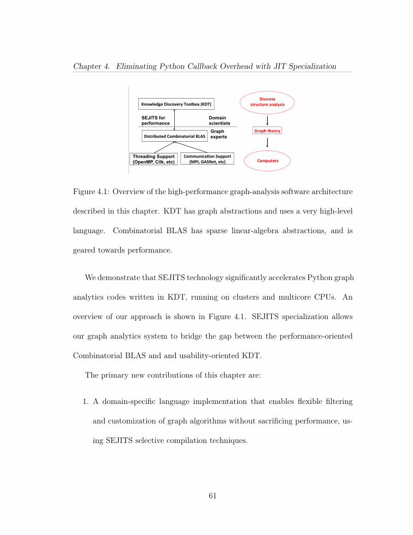
Chapter 4. Eliminating Python Callback Overhead with JIT Specialization
!"#$%&'&(#'%)$')%&(*+*,-#"#(
.%*/0('0&1%-(
213/)'&%#(2133)+"$*41+(5)//1%'(
6789:(.;5<&':(&'$=(
!"#'%">)'&?(213>"+*'1%"*,(@A;5(
Threading Support (OpenMP, Cilk, etc)
Graph experts
Domain scientists
B+1C,&?D&(!"#$1E&%-(F11,>1G(6B!F=(
SEJITS for performance
Graph Analysis Methodology
Figure 4.1: Overview of the high-performance graph-analysis software architecture
described in this chapter. KDT has graph abstractions and uses a very high-level
language. Combinatorial BLAS has sparse linear-algebra abstractions, and is
geared towards performance.
We demonstrate that SEJITS technology significantly accelerates Python graph
analytics codes written in KDT, running on clusters and multicore CPUs. An
overview of our approach is shown in Figure 4.1. SEJITS specialization allows
our graph analytics system to bridge the gap between the performance-oriented
Combinatorial BLAS and and usability-oriented KDT.
The primary new contributions of this chapter are:
1. A domain-specific language implementation that enables flexible filtering
and customization of graph algorithms without sacrificing performance, us-
ing SEJITS selective compilation techniques.
61
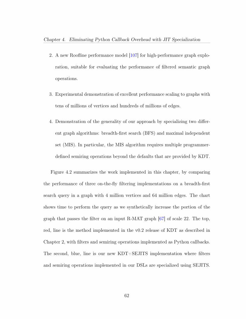
Chapter 4. Eliminating Python Callback Overhead with JIT Specialization
2. A new Roofline performance model [107] for high-performance graph explo-
ration, suitable for evaluating the performance of filtered semantic graph
operations.
3. Experimental demonstration of excellent performance scaling to graphs with
tens of millions of vertices and hundreds of millions of edges.
4. Demonstration of the generality of our approach by specializing two differ-
ent graph algorithms: breadth-first search (BFS) and maximal independent
set (MIS). In particular, the MIS algorithm requires multiple programmer-
defined semiring operations beyond the defaults that are provided by KDT.
Figure 4.2 summarizes the work implemented in this chapter, by comparing
the performance of three on-the-fly filtering implementations on a breadth-first
search query in a graph with 4 million vertices and 64 million edges. The chart
shows time to perform the query as we synthetically increase the portion of the
graph that passes the filter on an input R-MAT graph [67] of scale 22. The top,
red, line is the method implemented in the v0.2 release of KDT as described in
Chapter 2, with filters and semiring operations implemented as Python callbacks.
The second, blue, line is our new KDT+SEJITS implementation where filters
and semiring operations implemented in our DSLs are specialized using SEJITS.
62
Chapter 4. Eliminating Python Callback Overhead with JIT Specialization
0.1
1
10
1% 10% 100%
Me
an
BF
S T
ime
(se
co
nd
s,
log
sca
le)
Filter Permeability
KDTKDT+SEJITS
CombBLAS
Figure 4.2: Performance of a filtered BFS query, comparing three methods of
implementing custom semiring operations and on-the-fly filters. The vertical
axis is running time in seconds on a log scale; lower is better. From top to
bottom, the methods are: high-level Python filters and semiring operations in
KDT; high-level Python filters and semiring operations specialized at runtime
by KDT+SEJITS (this chapter’s main contribution); low-level C++ filters im-
plemented as customized semiring operations and compiled into Combinatorial
BLAS. The runs use 36 cores (4 sockets) of Intel Xeon E7-8870 processors.
This new implementation shows minimal overhead and comes very close to the
performance of native Combinatorial BLAS, which is in the third, gold line.
The rest of the chapter is organized as follows. Section 4.2 gives background
on the graph-analytical systems our work targets and builds upon. Section 4.3
is the technical heart of the chapter, which describes how we meet performance
challenges by using selective, embedded, just-in-time specialization. Section 4.4
63
Chapter 4. Eliminating Python Callback Overhead with JIT Specialization
presents Python-defined objects that enable the user to declare attribute types
directly in Python, enabling a broad set of applications. Section 4.6 proposes
a theoretical model that can be used to evaluate the performance of our imple-
mentations, giving “Roofline” bounds on the performance of breadth-first search
in terms of architectural parameters of a parallel machine, and the permeability
of the filter (that is, the percentage of edges that pass the filter). Section 4.5
gives details about the experimental setting and Section 4.7 presents our experi-
mental results. In Section 4.8, we precisely analyze the performance implications
of selective just-in translation using hardware performance counters. We survey
related work in Section 4.9. Section 4.10 gives our conclusions and some remarks
on future directions and problems.
4.2 Background
Running Example: Throughout the chapter, we will use a running example
query to show how different implementations of filters and semiring operations ex-
press the query and compare their performance executing it. We consider a graph
whose vertices are Twitter users, and whose edges represent two different types of
relationships between users. In the first type, one user “follows” another; in the
second type, one user “retweets” another user’s tweet. Each retweet edge carries
64
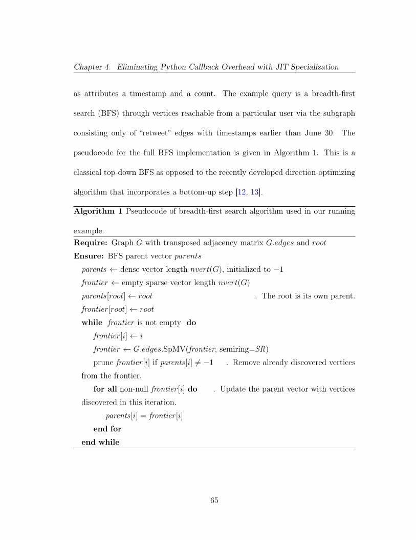
Chapter 4. Eliminating Python Callback Overhead with JIT Specialization
as attributes a timestamp and a count. The example query is a breadth-first
search (BFS) through vertices reachable from a particular user via the subgraph
consisting only of “retweet” edges with timestamps earlier than June 30. The
pseudocode for the full BFS implementation is given in Algorithm 1. This is a
classical top-down BFS as opposed to the recently developed direction-optimizing
algorithm that incorporates a bottom-up step [12, 13].
Algorithm 1 Pseudocode of breadth-first search algorithm used in our running
example.Require: Graph G with transposed adjacency matrix G.edges and root
Ensure: BFS parent vector parents
parents ← dense vector length nvert(G), initialized to −1frontier ← empty sparse vector length nvert(G)
parents [root]← root . The root is its own parent.
frontier [root]← root
while frontier is not empty do
frontier [i]← i
frontier ← G.edges.SpMV(frontier, semiring=SR)
prune frontier [i] if parents [i] 6= −1 . Remove already discovered vertices
from the frontier.
for all non-null frontier [i] do . Update the parent vector with vertices
discovered in this iteration.
parents [i] = frontier [i]
end for
end while
65
Chapter 4. Eliminating Python Callback Overhead with JIT Specialization
4.2.1 Filters As Scalar Semiring Operations
In this section, we show how a filter can be implemented below the KDT
level, as a user-specified semiring operation in the C++/MPI Combinatorial BLAS
library that underlies KDT. This is a path to high performance at the cost of
usability: the analyst must translate the graph-attribute definition of the filter
into low-level C++ code for custom semiring scalar operations in Combinatorial
BLAS.
The Combinatorial BLAS (CombBLAS for short) views graph computations as
sparse matrix computations using various algebraic semirings, such as the tropical
(min,+) semiring for shortest paths, or the real (+,*) semiring/field for numerical
computation. A semiring consists of a set of ‘scalars’, and two operations called
‘addition’ and ‘multiplication’. The semiring additive identity (SAID for short) is
also the multiplicative annihilator. The addition operation is commutative, and
both multiplication and addition are associative. Speaking generally about graph
algorithms, the ‘scalars’ are the edge and vertex data (attributes), ‘multiplica-
tion’ determines how the data on a sequence of edges are combined to represent a
path, and ‘addition’ determines how to combine two or more parallel paths. The
scalar multiply function is called for each edge examination, making it a suitable
candidate to embed the filtering logic. Two fundamental kernels in CombBLAS,
sparse matrix-vector multiplication (SpMV) and sparse matrix-matrix multiplica-
66
Chapter 4. Eliminating Python Callback Overhead with JIT Specialization
tion (SpGEMM), both use semirings to explore the graph by expanding existing
frontier(s) by a single hop.
The expert user can define new semirings and operations on them in C++
at the CombBLAS level, but most KDT users do not have the expertise for this.
Figure 4.3 shows the semiring for our running example of BFS on a Twitter graph.
The usual semiring multiply for BFS is select2nd, which returns the second value
it is passed; the multiply operation is modified to only return the second value
if the filter succeeds. At the lowest levels of SpMV, SpGEMM, and the other
CombBLAS primitive, the return value of the scalar multiply is checked against
SAID (in this example, the default constructed ParentType object is the additive
identity), and the returned object is retained only if it does not match the SAID.
Filters written as semiring operations in C++ can have high performance be-
cause the filter itself is a local operation that uses only the data on one edge,
and the number of calls to the filter operations is asymptotically the same as the
minimum necessary calls to the semiring scalar multiply, which itself is called once
per edge examination. The filtered multiply returns SAID if the predicate is not
satisfied.
67
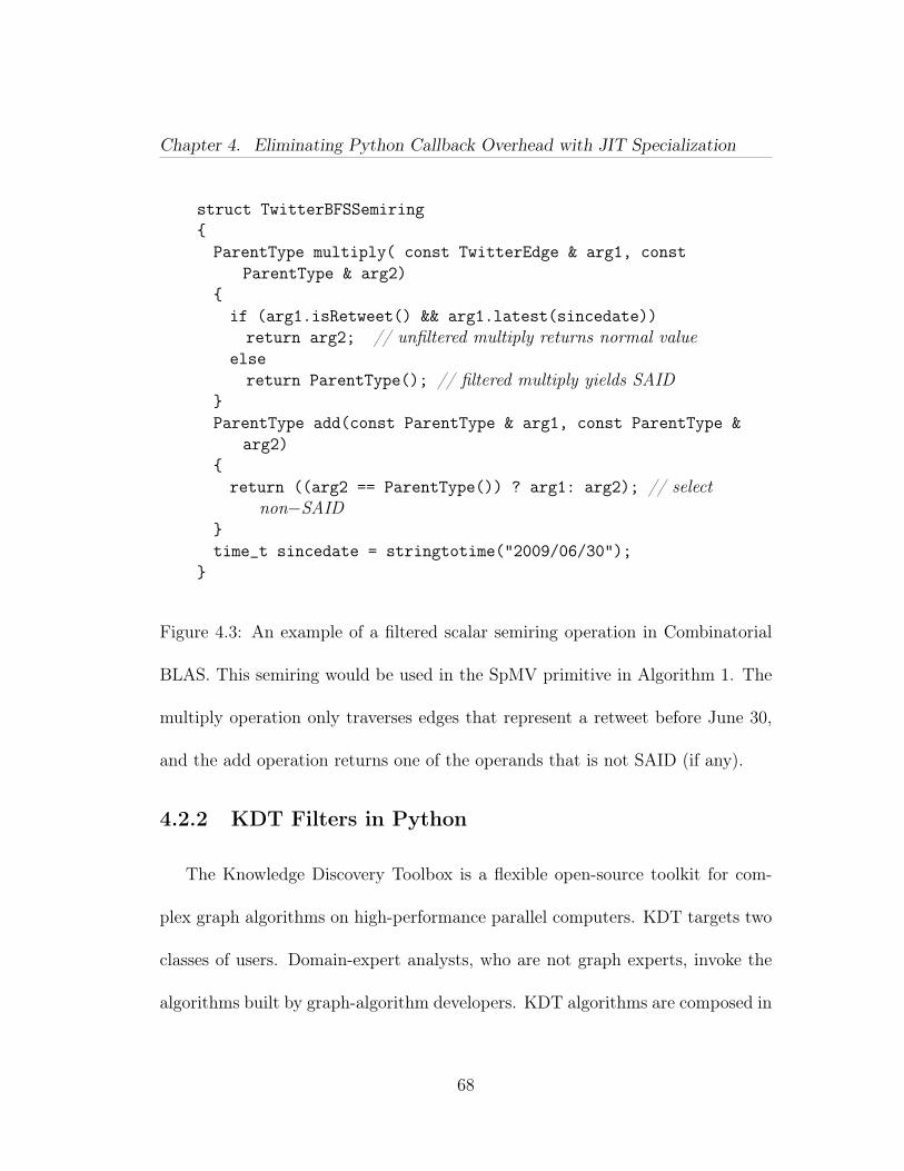
Chapter 4. Eliminating Python Callback Overhead with JIT Specialization
struct TwitterBFSSemiring{ParentType multiply( const TwitterEdge & arg1, const
ParentType & arg2){if (arg1.isRetweet() && arg1.latest(sincedate))return arg2; // unfiltered multiply returns normal value
elsereturn ParentType(); // filtered multiply yields SAID
}ParentType add(const ParentType & arg1, const ParentType &
arg2){return ((arg2 == ParentType()) ? arg1: arg2); // select
non−SAID}time_t sincedate = stringtotime("2009/06/30");
}
Figure 4.3: An example of a filtered scalar semiring operation in Combinatorial
BLAS. This semiring would be used in the SpMV primitive in Algorithm 1. The
multiply operation only traverses edges that represent a retweet before June 30,
and the add operation returns one of the operands that is not SAID (if any).
4.2.2 KDT Filters in Python
The Knowledge Discovery Toolbox is a flexible open-source toolkit for com-
plex graph algorithms on high-performance parallel computers. KDT targets two
classes of users. Domain-expert analysts, who are not graph experts, invoke the
algorithms built by graph-algorithm developers. KDT algorithms are composed in
68
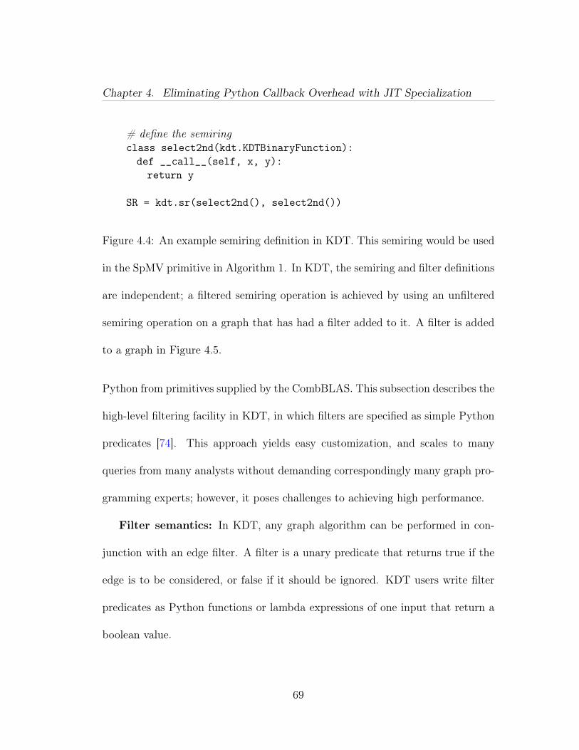
Chapter 4. Eliminating Python Callback Overhead with JIT Specialization
# define the semiringclass select2nd(kdt.KDTBinaryFunction):def __call__(self, x, y):return y
SR = kdt.sr(select2nd(), select2nd())
Figure 4.4: An example semiring definition in KDT. This semiring would be used
in the SpMV primitive in Algorithm 1. In KDT, the semiring and filter definitions
are independent; a filtered semiring operation is achieved by using an unfiltered
semiring operation on a graph that has had a filter added to it. A filter is added
to a graph in Figure 4.5.
Python from primitives supplied by the CombBLAS. This subsection describes the
high-level filtering facility in KDT, in which filters are specified as simple Python
predicates [74]. This approach yields easy customization, and scales to many
queries from many analysts without demanding correspondingly many graph pro-
gramming experts; however, it poses challenges to achieving high performance.
Filter semantics: In KDT, any graph algorithm can be performed in con-
junction with an edge filter. A filter is a unary predicate that returns true if the
edge is to be considered, or false if it should be ignored. KDT users write filter
predicates as Python functions or lambda expressions of one input that return a
boolean value.
69
Chapter 4. Eliminating Python Callback Overhead with JIT Specialization
Using a filter does not require any change in the code for the graph algorithm.
For example, KDT code for betweenness centrality or for breadth-first search is
the same whether or not the input semantic graph is filtered. Instead, the filtering
occurs in the low-level primitives. Our design allows all current and future KDT
algorithms to support filters without additional effort on the part of algorithm
designers. To implement our running example we define the semiring in Figure 4.4.
In Figure 4.5 we define an edge filter and add it to the graph.
It is possible in KDT to add multiple filters to a graph. The result is a nested
filter whose predicate is a lazily-evaluated “logical and” of the individual filter
predicates. Filters are evaluated in the order they are added. Multiple filter
support allows both end users and algorithm designers to use filters for their own
purposes.
Filtering approaches: KDT supports two approaches for filtering semantic
graphs:
• Materializing filter: When a filter is placed on a graph (or matrix or vector),
the entire graph is traversed and a copy is made that includes only edges
that pass the filter. We refer to this approach as materializing the filtered
graph.
70
Chapter 4. Eliminating Python Callback Overhead with JIT Specialization
• On-the-fly filter: No copy of the graph/matrix/vector is made. Rather,
every primitive operation (e.g. semiring scalar multiply and add) applies the
filter to its inputs when called. Roughly speaking, every primitive operation
accesses the graph through the filter and behaves as if the filtered-out edges
were not present.
Both materializing and on-the-fly filters have their place; neither is superior in
every situation. For example, materialization may be more efficient when running
many analyses on a well-defined small subset of a large graph. On the other hand,
materialization may be impossible if the graph already fills most of memory; and
materialization may be much more expensive than on-the-fly filtering for a query
whose filter restricts it to a localized neighborhood and thus does not even touch
most of the graph. Indeed, an analyst who needs to modify and fine-tune a filter
while exploring data may not be willing to wait for materialization at every step.
A key focus of this chapter is on-the-fly filtering and making it more efficient.
Our experiments demonstrate that materializing the subgraph can take as much
as 18 times the time of performing a single BFS on the largest of the real twitter
datasets. In this comparison, both materialization (an embarrassingly parallel
task) and the BFS are run in parallel using 36 cores of Intel Xeon E7-8870.
Implementation details: Filtering a semiring operation requires the semir-
ing scalar multiply to be able to return “null”, in the sense that the result should
71
Chapter 4. Eliminating Python Callback Overhead with JIT Specialization
# G is a kdt.DiGraphclass TwitterFilter(kdt.KDTUnaryPredicate):def __call__(self, e):return (e.count > 0 and e.latest <
str_to_date("2009/06/30"))
earlyRetweetsOnly = TwitterFilter()
G.addEFilter(earlyRetweetsOnly)G.e.materializeFilter() # omit this line for on−the−fly filtering
# perform some operations or queries on G, such as BFS
G.delEFilter(earlyRetweetsOnly)
Figure 4.5: Adding and removing an edge filter in KDT, with or without materi-
alization.
be the same as if the multiply never occurred. In semiring terms, the multiply
operation must return the SAID. CombBLAS treats SAID the same as any other
value. However, CombBLAS uses a sparse data structure to represent the graph
as an adjacency matrix—and, formally speaking, SAID is the implicit value of
any matrix entry not stored explicitly.
CombBLAS ensures that SAID is never stored as an explicit value in a sparse
structure. This corresponds to Matlab’s convention that explicit zeros are never
stored in sparse matrices [42], and differs from the convention in the CSparse
sparse matrix package [28]. Note that SAID need not be “zero”: for example, in
72
Chapter 4. Eliminating Python Callback Overhead with JIT Specialization
the min-plus semiring used for shortest path computations, SAID is ∞. Indeed,
it is possible for a single graph or matrix to be used with different underlying
semirings whose operations use different SAIDs.
We benchmarked several approaches to representing, manipulating, and re-
turning SAID values from semiring scalar operations. It is crucial for usability to
allow filters to be ignorant of the semiring they are applied to; therefore, return-
ing a SAID needs to be an out-of-band signal. We pair each basic semiring scalar
operation with a returnedSAID() predicate which is called after the scalar opera-
tion. We use a predicate instead of a flag because the predicate can be optimized
out by the compiler for unfiltered operations.
The result is a clean implementation of on-the-fly filters: filtering a semiring
simply requires a small adapter code in the semiring multiply() function that
calls the filter predicate on both operands. If the predicate returns false for either
operand then the adapter causes returnedSAID() to return true. Otherwise the
semiring’s callback is called and its value returned.
73
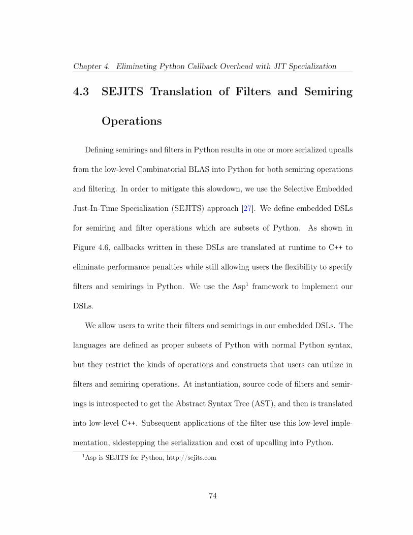
Chapter 4. Eliminating Python Callback Overhead with JIT Specialization
4.3 SEJITS Translation of Filters and Semiring
Operations
Defining semirings and filters in Python results in one or more serialized upcalls
from the low-level Combinatorial BLAS into Python for both semiring operations
and filtering. In order to mitigate this slowdown, we use the Selective Embedded
Just-In-Time Specialization (SEJITS) approach [27]. We define embedded DSLs
for semiring and filter operations which are subsets of Python. As shown in
Figure 4.6, callbacks written in these DSLs are translated at runtime to C++ to
eliminate performance penalties while still allowing users the flexibility to specify
filters and semirings in Python. We use the Asp1 framework to implement our
DSLs.
We allow users to write their filters and semirings in our embedded DSLs. The
languages are defined as proper subsets of Python with normal Python syntax,
but they restrict the kinds of operations and constructs that users can utilize in
filters and semiring operations. At instantiation, source code of filters and semir-
ings is introspected to get the Abstract Syntax Tree (AST), and then is translated
into low-level C++. Subsequent applications of the filter use this low-level imple-
mentation, sidestepping the serialization and cost of upcalling into Python.1Asp is SEJITS for Python, http://sejits.com
74
Chapter 4. Eliminating Python Callback Overhead with JIT Specialization
KDT Algorithm
CombBLAS Primi4ve
Filter (Py)
Python
C++
Semiring (Py) KDT Algorithm
CombBLAS Primi4ve Filter (C++)
Semiring (C++)
Standard KDT KDT+SEJITS
SEJITS Transla4on
Filter (Py)
Semiring (Py)
Figure 4.6: Left: Calling process for filter and semiring operations in KDT. For
each edge, the C++ infrastructure must upcall into Python to execute the callback.
Right: Using our DSLs, the C++ infrastructure calls the translated version of the
operation, eliminating the upcall overhead.
Although KDT is our target platform in this work, our specialization approach
can be used to accelerate other graph processing systems with similar performance
challenges. In the next sections, we define our domain-specific languages and show
several examples of using them from Python.
4.3.1 Python Syntax for the DSLs
We choose to implement two separate DSLs to clearly express and restrict
the kinds of computations that can be done with each; for example, filters require
boolean return values, while semiring operations require return values that are one
of the vertex or edge types. Separating out the languages and their forms allows
75
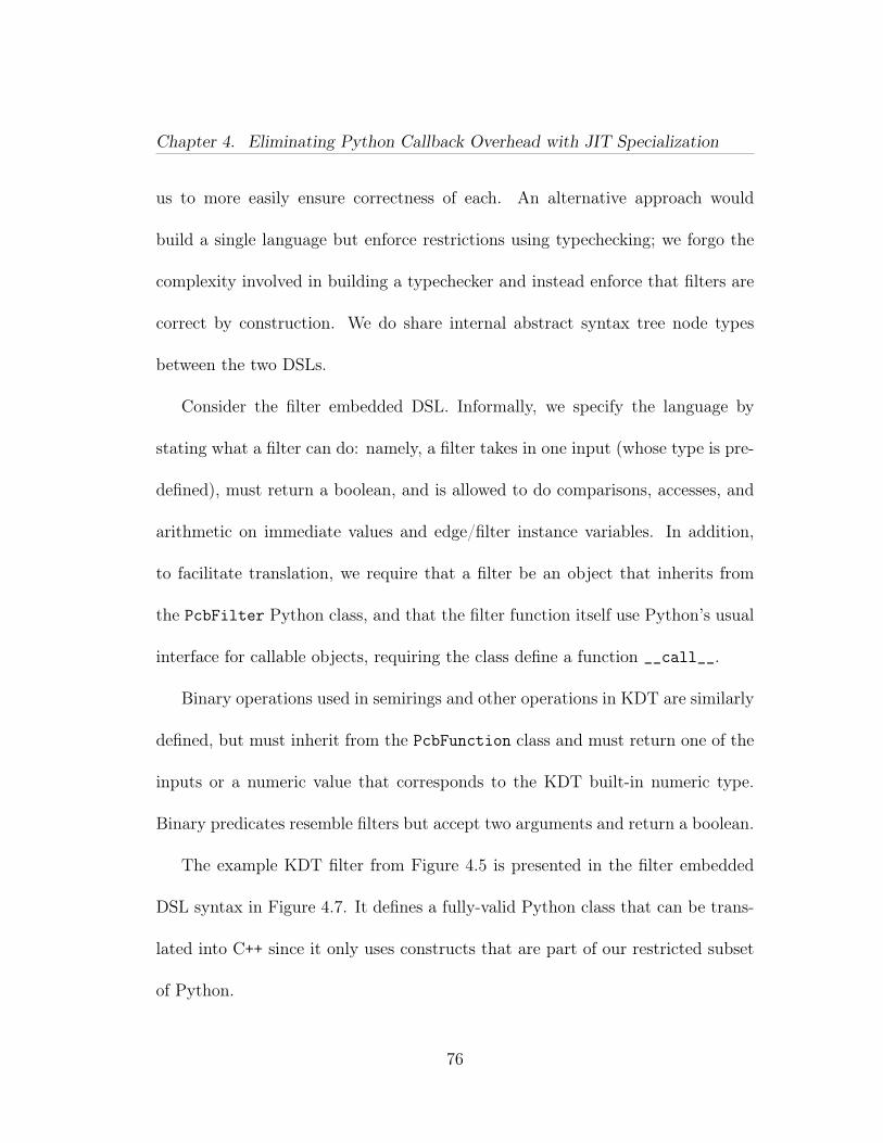
Chapter 4. Eliminating Python Callback Overhead with JIT Specialization
us to more easily ensure correctness of each. An alternative approach would
build a single language but enforce restrictions using typechecking; we forgo the
complexity involved in building a typechecker and instead enforce that filters are
correct by construction. We do share internal abstract syntax tree node types
between the two DSLs.
Consider the filter embedded DSL. Informally, we specify the language by
stating what a filter can do: namely, a filter takes in one input (whose type is pre-
defined), must return a boolean, and is allowed to do comparisons, accesses, and
arithmetic on immediate values and edge/filter instance variables. In addition,
to facilitate translation, we require that a filter be an object that inherits from
the PcbFilter Python class, and that the filter function itself use Python’s usual
interface for callable objects, requiring the class define a function __call__.
Binary operations used in semirings and other operations in KDT are similarly
defined, but must inherit from the PcbFunction class and must return one of the
inputs or a numeric value that corresponds to the KDT built-in numeric type.
Binary predicates resemble filters but accept two arguments and return a boolean.
The example KDT filter from Figure 4.5 is presented in the filter embedded
DSL syntax in Figure 4.7. It defines a fully-valid Python class that can be trans-
lated into C++ since it only uses constructs that are part of our restricted subset
of Python.
76
Chapter 4. Eliminating Python Callback Overhead with JIT Specialization
class MyFilter(PcbFilter):def __init__(self, ts):self.ts = ts
def __call__(self, e):# if it is a retweet edgeif (e.isRetweet and
# and it is before our initialized timestampe.latest < self.ts):
return Trueelse:return False
Figure 4.7: Example of an edge filter that the translation system can convert
from Python into fast C++ code. Note that the timestamp in question is passed
in at filter instantiation time.
4.3.2 Translating User-Defined Filters and Semiring Oper-
ations
In the Asp framework for SEJITS embedded DSLs, the most important mech-
anism for ensuring correct translations is to create an intermediate representation,
called the semantic model, which defines the semantics of valid translatable ob-
jects. AST nodes from parsing Python are translated into this intermediate form
as a first step of translation, and most of the logic for checking whether the defini-
tion is translatable is executed in this first phase. To be clear, this representation
77
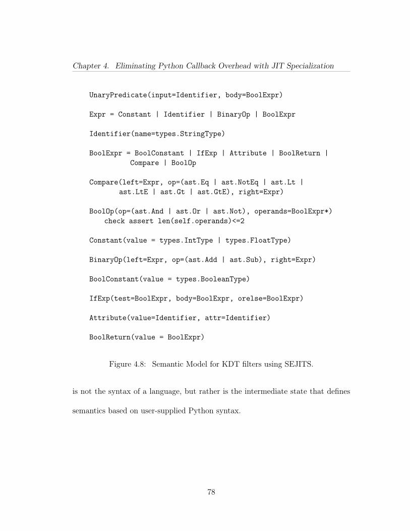
Chapter 4. Eliminating Python Callback Overhead with JIT Specialization
UnaryPredicate(input=Identifier, body=BoolExpr)
Expr = Constant | Identifier | BinaryOp | BoolExpr
Identifier(name=types.StringType)
BoolExpr = BoolConstant | IfExp | Attribute | BoolReturn |Compare | BoolOp
Compare(left=Expr, op=(ast.Eq | ast.NotEq | ast.Lt |ast.LtE | ast.Gt | ast.GtE), right=Expr)
BoolOp(op=(ast.And | ast.Or | ast.Not), operands=BoolExpr*)check assert len(self.operands)<=2
Constant(value = types.IntType | types.FloatType)
BinaryOp(left=Expr, op=(ast.Add | ast.Sub), right=Expr)
BoolConstant(value = types.BooleanType)
IfExp(test=BoolExpr, body=BoolExpr, orelse=BoolExpr)
Attribute(value=Identifier, attr=Identifier)
BoolReturn(value = BoolExpr)
Figure 4.8: Semantic Model for KDT filters using SEJITS.
is not the syntax of a language, but rather is the intermediate state that defines
semantics based on user-supplied Python syntax.
78
Chapter 4. Eliminating Python Callback Overhead with JIT Specialization
In filters and semirings, the user may wish to inspect fields of the input data
types, do comparisons, and perhaps perform arithmetic with fields. Consequently
our semantic model allows these operations.
On the other hand, we want to (as much as possible) prevent users from
writing code that does not conform to our assumptions; although we could use
analysis for this, it is much simpler to construct the languages in a manner that
prevents users from writing non-conformant code in either embedded DSL. If the
filter or semiring operation does not fit into our language, we run it in the usual
fashion, by doing upcalls into pure Python, after outputting a warning. Thus,
if the user writes their code correctly, they achieve fast performance, otherwise
the user experience is no worse than before— the code still runs, just not at fast
speed.
The semantic models are shown in Figures 4.8 and 4.9. We have defined it
to make it easy to write filters and operations that are “correct by construction”;
that is, if they fit into the semantic model, they follow the restrictions of what can
be translated. For example, for filters, we require that the return be provably a
boolean (by forcing the BoolReturn node to have a boolean body), and that there
be either a single input or two inputs (either UnaryPredicate or BinaryPredicate).
The semantic model for semiring operations ensures the returned item is one of
the inputs or an elemental type understood by KDT.
79
Chapter 4. Eliminating Python Callback Overhead with JIT Specialization
We define tree transformations that dictate how Python AST nodes are trans-
lated into semantic model nodes. For example, the Python function definition
for __call__ is translated into a UnaryPredicate node in the case of the filter
embedded DSL. Similarly, in the filter embedded DSL, the transformation checks
whether the body of the return statement is provably a boolean and returns a
BooleanReturn node.
After the code is translated into instances of the semantic model, the rest
of the translation is straightforward, utilizing Asp’s infrastructure for converting
semantic models into backend code. For many of these transformations, defaults
built into Asp are sufficient; for example, we leverage the default translation for
constant numbers and therefore do not need to define the transform. The end
result of conversion is source code containing the function in a private namespace
plus some glue code, described in the next section. This source is passed to
CodePy, which compiles it into a small dynamically linked library that is then
automatically loaded into the running interpreter.
4.3.3 Implementation in C++
We modify the C++ portion of KDT’s callback mechanism which is based
on pointers to Python functions. We add an additional function pointer that
is checked before executing the upcall to Python. This function pointer is set
80
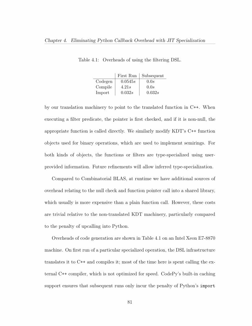
Chapter 4. Eliminating Python Callback Overhead with JIT Specialization
Table 4.1: Overheads of using the filtering DSL.
First Run SubsequentCodegen 0.0545s 0.0sCompile 4.21s 0.0sImport 0.032s 0.032s
by our translation machinery to point to the translated function in C++. When
executing a filter predicate, the pointer is first checked, and if it is non-null, the
appropriate function is called directly. We similarly modify KDT’s C++ function
objects used for binary operations, which are used to implement semirings. For
both kinds of objects, the functions or filters are type-specialized using user-
provided information. Future refinements will allow inferred type-specialization.
Compared to Combinatorial BLAS, at runtime we have additional sources of
overhead relating to the null check and function pointer call into a shared library,
which usually is more expensive than a plain function call. However, these costs
are trivial relative to the non-translated KDT machinery, particularly compared
to the penalty of upcalling into Python.
Overheads of code generation are shown in Table 4.1 on an Intel Xeon E7-8870
machine. On first run of a particular specialized operation, the DSL infrastructure
translates it to C++ and compiles it; most of the time here is spent calling the ex-
ternal C++ compiler, which is not optimized for speed. CodePy’s built-in caching
support ensures that subsequent runs only incur the penalty of Python’s import
81
Chapter 4. Eliminating Python Callback Overhead with JIT Specialization
statement. On a multi-processor machine, only one process performs the compi-
lation; the remaining ones load the cached version when that single compilation
finishes.
4.4 Attributes defined in Python and exposed to
C++
4.4.1 Motivation
The attribute types of vertices and edges should ideally be declared in Python,
especially when the application requires several graphs with different edge and/or
vertex datatypes. Consider the analysis of multi-modal brain networks (also
known as connectomes). In this application, data from multiple modalities, such
as fMRI, DTI, EEG, and PET, are collected for the patient’s brain. Representing
these data sources as graphs and using graph analysis has been instrumental in
characterizing neurodegenerative diseases. The co-registration of these modali-
ties requires the application to handle multiple graphs with different edge/vertex
types. For example, the temporal and spatial resolution of fMRI and EEG data
are incompatible [84], requiring different vertex types. Similarly, the voxel cor-
relations in fMRI and DTI are defined differently, requiring different edge types.
82
Chapter 4. Eliminating Python Callback Overhead with JIT Specialization
The ability to declare edge and vertex types dynamically in Python allows co-
analysis of different brain networks and overcomes the limitations of using a single
modality [64], and we plan to leverage our described methodology for forthcoming
investigations of computational neuropathology.
4.4.2 Challenge
We wish to enable the user to declare attribute types in Python. However,
in order to obtain high-performance we must meet some CombBLAS and MPI
requirements. CombBLAS’s architecture requires that all elements of a matrix
or vector must have the same type and size. These elements, or Python-Defined
Objects (PDOs), must have the following properties:
• Self contained: no external references, object must be able to be copied by
value (i.e. with memcpy).
• Object is declared and accessed in Python, memory is allocated in C++.
• Python-defined structure must be able to be operated on in C++
KDT 0.3 introduces just such a scheme. We declare a structure in Python
that is then placed within a buffer of raw bytes. In other words, we turn C++
objects Obj1 and Obj2 into void* buffers which are in effect typecast to the
Python-defined type at runtime.
83
Chapter 4. Eliminating Python Callback Overhead with JIT Specialization
4.4.3 Structure Declaration
Python’s ctypes interface is used to call into C libraries. Since some C func-
tions operate on struct datatypes, ctypes includes mechanisms to declare a
C struct in Python. ctypes exposes C primitive datatypes such as c_int or
c_double which can be composed together into a struct which is binary com-
patible with compiled C code on that particular system. We expose a subset of
ctypes’s datatypes to the KDT user to use to declare a Python-Defined Object’s
data members.
Python access to the PDO is handled via ctypes’s hooks, which enable the
structure to behave like any Python object. Python operators can be declared
using Python’s standard operator definition machinery.
A simple example of a custom edge type is a PDO version of the structure in
Figure 4.10, as follows:
class TwitterEdge(Structure):_fields_ = [("follower", c_bool),
("latest", c_uint64), # time_t("count", c_short)]
4.4.4 Memory Handling
CombBLAS is not aware that it is working with a Python-Defined Object;
instead, what it sees is a byte buffer of a fixed size. Therefore, all memory for
84
Chapter 4. Eliminating Python Callback Overhead with JIT Specialization
PDOs is allocated by CombBLAS. Pointers to this memory are passed to the
callbacks, which then use ctypes’s mechanisms to create a Python object backed
by the CombBLAS buffer. The PDO is then accessible in the Python callback.
4.4.5 PDOs and SEJITS
For SEJITS to support the PDO it must be able to access the PDO’s memory
in the same way as the Python operations would. Luckily ctypes declares the
structure in precisely such a way. We translate all PDO structs used by a spe-
cialized callback into C and add the declarations to the SEJITS-generated C++
module. The callback’s parameters are the buffer objects, Obj1 and/or Obj2. We
add code to extract the buffers and typecast them to references to the particular
structs that the buffers correspond to.
The rest of the C++ specialized callback can now operate on the buffer as if it
were a struct.
4.4.6 Limitations
Our approach has some limitations, namely that we can only support the
intersection of Python and C++ language features. In particular, data members
and their types must be declared ahead of time. The declaration is decidedly
85
Chapter 4. Eliminating Python Callback Overhead with JIT Specialization
C-style, and any duck-typed definitions will be lost. The PDO must not contain
any pointers or references.
CombBLAS requires that the datatypes must be copyable by value for MPI
communication, so no copy constructors are called. In addition, the size of the
buffers must be declared at compile time. Our scheme allows an unlimited number
of different PDO types to be declared in a single program, but each one must fit
into one of a handful different buffer sizes.
4.5 Experimental Design
This section describes the graph algorithms used in our experiments, the
benchmark matrices we used to test the algorithms, and the machines on which we
ran our tests. KDT version 0.3 is enabled with the SEJITS techniques described
in this chapter, and is freely available at http://kdt.sourceforge.net.
4.5.1 Algorithms Considered
Our first algorithm is a filtered graph traversal. Given a vertex of interest, it
determines the number of hops required to reach every other vertex using only
those retweet edges timestamped earlier than a given date. The filter in this case
is a boolean predicate on edge attributes that defines the types and timestamps
86
Chapter 4. Eliminating Python Callback Overhead with JIT Specialization
of the edges to be used. The query is a breadth-first search (BFS) on the graph
that ignores edges that do not pass the filter.
Our second query is to find the maximal independent set (MIS) of this graph.
MIS finds a subset of vertices such that no two members of the subset are con-
nected to each other and all other vertices outside MIS are connected to at least
one member of the MIS. Since MIS is defined on an undirected graph, we first
ignore edge directions, then we execute Luby’s randomized parallel algorithm [70]
implemented in KDT. The filter is the same as in the first query.
4.5.2 Test Data Sets
We evaluate our techniques on both algorithms using synthetically-generated
graphs and those that are based on real data sets. Our BFS experiments using the
synthetic data are generated based on the R-MAT model [67] that can generate
graphs with a highly skewed degree distribution. An R-MAT graph of scale N
has 2N vertices and approximately edgefactor ·2N edges. In our tests, edgefactor
is 16, and R-MAT seed parameters a, b, c, and d are 0.57, 0.19, 0.19, and 0.05.
After generating this non-semantic (boolean) graph, edge payloads are artificially
introduced with timestamp values generated using the Mersenne Twister pseudo-
random number generator [80]. A simple threshold controls filter permeability.
We use a fixed seed so that the experiments are reproducible and all codes work
87
Chapter 4. Eliminating Python Callback Overhead with JIT Specialization
on the same problem. The edge type is the same as the Twitter edge type
described in the next paragraph in order to be consistent between experiments on
real and synthetic data. Our MIS experiments use Erdős-Rényi graphs [37] with an
edgefactor of 4 because the MIS algorithm on R-MAT graphs completes in very
few steps due to high coupling and would not yield a meaningful performance
analysis.
Our real data graphs are based on social network interactions, using anonymized
Twitter data [60, 111]. In our Twitter graphs, edges can represent two different
types of interactions. The first interaction is the “following” relationship, where
an edge from vertex vi to vj implies that vi is following vj (note that these direc-
tions are consistent with the common authority-hub definitions in the World Wide
Web). The second interaction encodes an abbreviated “retweet” relationship: an
edge from vi to vj implies that vi has mentioned vj at least once in tweets. The
edge also keeps the count of such tweets as well as the last tweet date if the count
is larger than one.
The tweets occurred in the period of June-December of 2009. To allow scaling
studies, we created subsets of these tweets based on the date they occur. The
small dataset contains tweets from the first two weeks of June, the medium dataset
contains tweets from June and July, the large dataset contains tweets dated June
through September, and finally the huge dataset contains all the tweets from June
88
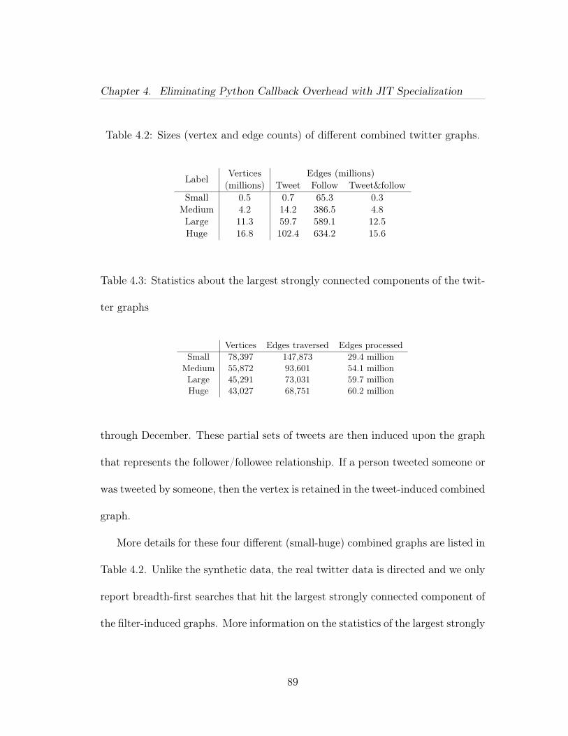
Chapter 4. Eliminating Python Callback Overhead with JIT Specialization
Table 4.2: Sizes (vertex and edge counts) of different combined twitter graphs.
Label Vertices Edges (millions)(millions) Tweet Follow Tweet&follow
Small 0.5 0.7 65.3 0.3Medium 4.2 14.2 386.5 4.8Large 11.3 59.7 589.1 12.5Huge 16.8 102.4 634.2 15.6
Table 4.3: Statistics about the largest strongly connected components of the twit-
ter graphs
Vertices Edges traversed Edges processedSmall 78,397 147,873 29.4 million
Medium 55,872 93,601 54.1 millionLarge 45,291 73,031 59.7 millionHuge 43,027 68,751 60.2 million
through December. These partial sets of tweets are then induced upon the graph
that represents the follower/followee relationship. If a person tweeted someone or
was tweeted by someone, then the vertex is retained in the tweet-induced combined
graph.
More details for these four different (small-huge) combined graphs are listed in
Table 4.2. Unlike the synthetic data, the real twitter data is directed and we only
report breadth-first searches that hit the largest strongly connected component of
the filter-induced graphs. More information on the statistics of the largest strongly
89
Chapter 4. Eliminating Python Callback Overhead with JIT Specialization
connected components of the graphs can be found in Table 4.3. Processed edge
count includes both the edges that pass the filter and the edges that are filtered
out.
4.5.3 Architectures
To evaluate our methodology, we examine graph analysis behavior on Mirasol,
an Intel Nehalem-based machine, as well as Hopper, a Cray XE6 supercomputer
at NERSC. Mirasol is a single node platform composed of four Intel Xeon E7-
8870 processors. Each socket has ten cores running at 2.4 GHz, and supports
two-way simultaneous multithreading (20 thread contexts per socket). The cores
are connected to a very large 30 MB L3 cache via a ring architecture. The sus-
tained STREAM [81] bandwidth is about 30 GB/s per socket. The machine has
256 GB of DDR3-1066 DRAM. We utilize a flat MPI programming modeling using
OpenMPI 1.4.3 with GCC C++ compiler version 4.4.5, and Python 2.6.6.
Hopper is a Cray XE6 massively parallel processing (MPP) system, built from
dual-socket 12-core “Magny-Cours” Opteron compute nodes. Each socket (multi-
chip module) has two 6-core chips, so a node can be viewed as a four-chip com-
pute configuration with strong NUMA properties. Each Opteron chip contains
six super-scalar, out-of-order cores capable of completing one (dual-slot) SIMD
add and one SIMD multiply per cycle. Additionally, each core has private 64 KB
90
Chapter 4. Eliminating Python Callback Overhead with JIT Specialization
L1 and 512 KB low-latency L2 caches. The six cores on a chip share a 6MB L3
cache and dual DDR3-1333 memory controllers capable of providing an average
STREAM bandwidth of 12GB/s per chip. Each pair of compute nodes shares
one Gemini network chip that collectively form a 3D torus. We use Cray’s MPI
implementation, which is based on MPICH2, and compile our code with GCC
C++ compiler version 4.6.2 and Python 2.7. Complicating our experiments, some
compute nodes of this MPP do not contain a compiler. To remedy this, we en-
sured that a compute node with access to the requisite compilers was used to build
the KDT+SEJITS filters, since the on-the-fly compilation mechanism requires at
least one MPI process be able to call the compilation toolchain.
4.6 A Roofline model of BFS
The Roofline model [107] is a visually intuitive representation of the perfor-
mance characteristics of a kernel on a specific machine. It uses bound and bottle-
neck analysis to delineate performance bounds arising from bandwidth or compute
limits and has been demonstrated to show that performance of many HPC ker-
nels is well-correlated with STREAM bandwidth. Unfortunately, the traditional
HPC application characteristics (massive parallelism, streaming memory access)
and even metrics (flops per byte) are often antithetical to the computational chal-
91
Chapter 4. Eliminating Python Callback Overhead with JIT Specialization
lenges found in linear algebra-based graph algorithms. To remedy this, we extend
the Roofline model to quantify the performance bounds of BFS as a function of
optimization and filter success rate. Doing so allowed us to separate the effects of
computation from data movement and express performance as a function of Filter
Permeability — the percentage of edges that pass the filter — and thus explain
the performance benefit of the technology demonstrated in this paper.
In order to model BFS performance, we decouple in-core compute limits (fil-
ter and semiring performance as measured in processed edges per second) from
memory access performance. The in-core filter performance limits were derived
by extracting the relevant CombBLAS, KDT, and SEJITS+KDT versions of the
kernels and applying them to arrays that fit in each core’s cache. We run the edge
processing inner kernels 10,000 times (as opposed to once) to amortize any mem-
ory system related effects to get the in-core compute limits. The compute limit
decreases with increasing permeability because two operations must be performed
for an edge that passes the filter as opposed to the one operation for an edge that
does not.
Analogous to arithmetic intensity, we can quantify the average number of bytes
we must transfer from DRAM per edge we process — bytes per processed edge.
To do so, we must not only estimate data movement, but also effective bandwidth
for each operation. In the following analysis, the indices are 8 bytes and the
92
Chapter 4. Eliminating Python Callback Overhead with JIT Specialization
edge payload is 16 bytes. BFS exhibits three memory access patterns which are
illustrated in Figure 4.11. First, there is a unit-stride streaming access pattern
arising from access of the vertex pointers (this is amortized by degree) as well as
the creation of the sparse output vector that acts as the new frontier (the gather
step in Figure 4.11). The latter incurs 32 bytes of traffic per traversed edge in
write-allocate caches assuming the edge was not filtered. Second, access to the
adjacency list follows a stanza-like memory access pattern. That is, small blocks
(stanzas) of consecutive elements are fetched from effectively random locations in
memory. These stanzas are typically less than the mean degree, due to two rea-
sons. The first reason is the heavy-tailed degree distribution that is characteristic
of many real world graph instances, which applies to both sequential and parallel
settings regardless of the data decomposition. In heavy-tailed distributions, the
median is smaller than mean. The second reason only applies to the parallel set-
ting and it is due to per-processor subgraphs being sparser than the full graph for
the 2D decomposition (also called hypersparsity [25]). The stanza related traffic
corresponds to approximately 24 bytes (16 for payload and 8 for index) of DRAM
traffic per processed edge. Finally, updates to the list of visited vertices (the
scatter/accumulate step in Figure 4.11) and the indirections when accessing the
graph data structure exhibit a memory access pattern in which effectively random
8 byte elements are updated (assuming the edge was not filtered). Similarly, each
93
Chapter 4. Eliminating Python Callback Overhead with JIT Specialization
visited vertex generates 24 bytes of random access traffic to follow indirections on
the graph structure before being able to access its edges.
In order to quantify these bandwidths, which we expect to be quite different
than STREAM, we wrote a custom micro-benchmark that provides stanza-like
memory access patterns (read or update) with spatial locality varying from 8
bytes (random access) to the size of the array (i.e. asymptotically the STREAM
benchmark).
The memory bandwidth requirements depend on the number of edges pro-
cessed (examined), number of edges traversed (that pass the filter), and the num-
ber of vertices in the frontier over all iterations. For instance, an update to the
list of visited vertices only happens if the edge actually passes the filter. Typi-
cally, the number of edges traversed is roughly equal to the permeability of the
filter times the number of edges processed. To get a more accurate estimate, we
collected statistics from one of the synthetically generated R-MAT graphs that
are used in our experiments. These statistics are summarized in Table 4.4. Simi-
larly, we quantify the volume of data movement by operation and memory access
type (random, stanza-like, and streaming) noting the corresponding bandwidth
on Mirasol, our Intel Xeon E7-8870 test system (see Section 4.5), in Table 4.5.
Combining Tables 4.4 and 4.5, we calculate the average number of processed edges
94
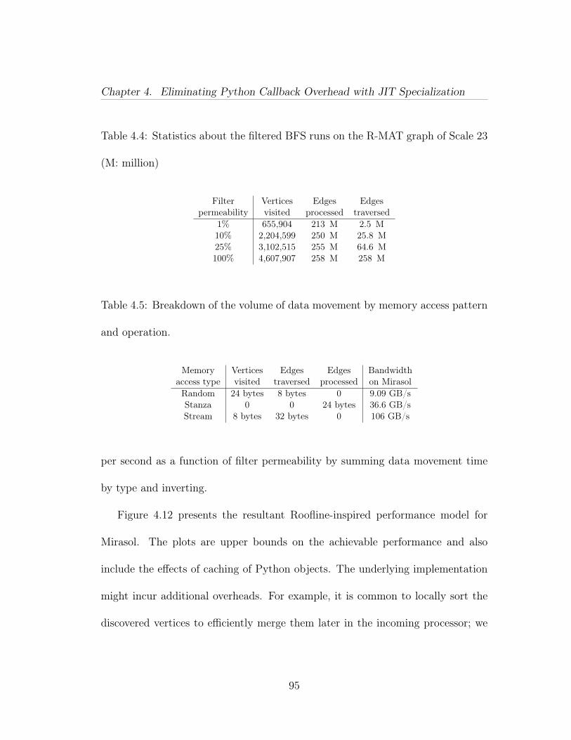
Chapter 4. Eliminating Python Callback Overhead with JIT Specialization
Table 4.4: Statistics about the filtered BFS runs on the R-MAT graph of Scale 23
(M: million)
Filter Vertices Edges Edgespermeability visited processed traversed
1% 655,904 213 M 2.5 M10% 2,204,599 250 M 25.8 M25% 3,102,515 255 M 64.6 M100% 4,607,907 258 M 258 M
Table 4.5: Breakdown of the volume of data movement by memory access pattern
and operation.
Memory Vertices Edges Edges Bandwidthaccess type visited traversed processed on MirasolRandom 24 bytes 8 bytes 0 9.09 GB/sStanza 0 0 24 bytes 36.6 GB/sStream 8 bytes 32 bytes 0 106 GB/s
per second as a function of filter permeability by summing data movement time
by type and inverting.
Figure 4.12 presents the resultant Roofline-inspired performance model for
Mirasol. The plots are upper bounds on the achievable performance and also
include the effects of caching of Python objects. The underlying implementation
might incur additional overheads. For example, it is common to locally sort the
discovered vertices to efficiently merge them later in the incoming processor; we
95
Chapter 4. Eliminating Python Callback Overhead with JIT Specialization
do not account for this overhead as it is not an essential step of the algorithm.
Neither access to MPI buffers nor MPI performance was taken into account.
The Roofline model selects ceilings by optimization, and bounds performance
by their minimum. We select a filter implementation (pure Python KDT, KDT+SEJITS,
or CombBLAS) and look for the minimum between that filter implementation’s
limit and the weighted DRAM bandwidth limit. We observe a pure Python KDT
filter will be the bottleneck in a BFS computation as it cannot sustain performance
(edges per second) at the rate the processor can move edges on-chip. Conversely,
the DRAM bandwidth performance limit is about 5× lower than the CombBLAS
in-core performance limit. Ultimately, the performance of a SEJITS specialized
filter is sufficiently fast to ensure a BFS implementation will be bandwidth-bound.
This crucial observation explains why KDT+SEJITS performance is so close to
CombBLAS performance in practice (as shown later in Section 4.7) even though
its in-core performance is about 2.6× slower.
This Roofline model serves as an excellent surrogate for the performance we
observe in practice in Figure 4.2 and generally in Section 4.7. Specifically, it
methodologically explains the smaller (≈40×) gap we observe between SEJITS
and pure Python KDT performances for BFS as opposed to over 140× suggested
by the in-core compute limits. The actual performance difference is the gap be-
tween the DRAM bandwidth limit and the KDT in-core compute limit because
96
Chapter 4. Eliminating Python Callback Overhead with JIT Specialization
the SEJITS Roofline is the lower of the bandwidth-bound and in-core compute-
bound lines. Due to the aforementioned data movement effects that we did not
account for (such as sorting and MPI buffers), the model suggests a slightly higher
bandwidth-bound line, hence a slightly bigger gap than what we observe in prac-
tice.
4.7 Experimental Results
In this section we use [semiring implementation]/[filter implementation] no-
tation to describe the various implementation combinations we compare. For
example, Python/SEJITS means that only the filter is specialized with SEJITS
but the semiring is in pure Python (not specialized).
4.7.1 Performance Effects of Permeability
Figure 4.13 shows the relative distributed-memory performance of four meth-
ods in performing breadth-first search on a graph with 32 million vertices and
512 million edges, with varying filter permeability. The structure of the input
graph is an R-MAT of scale 25, and the edges are artificially introduced so that
the specified percentage of edges pass the filter. These experiments are run on
Hopper using 576 MPI processes with one MPI process per core. The figure shows
97
Chapter 4. Eliminating Python Callback Overhead with JIT Specialization
that the SEJITS/SEJITS KDT implementation (blue line) closely tracks Comb-
BLAS performance (gold line), with the gap between it and the Python/Python
KDT implementation (red line) shrinking as permeability increases. This is ex-
pected because as the permeability increases, both implementations approach the
bandwidth bound regime as suggested by the Roofline model in Section 4.6.
A similar but more condensed figure, showing the performance effects of per-
meability on Mirasol (Figure 4.2) is in Section 4.1. There, KDT+SEJITS is the
same as SEJITS/SEJITS. The effects of permeability on the MIS performance are
shown in Figure 4.14 and reflect the BFS findings.
Since low permeability (1-10%) cases incur less memory traffic, Python over-
heads (KDT algorithms are implemented in Python) as well as the function pointer
chasing of the SEJITS approach leave a noticeable overhead over CombBLAS. This
is not the case for high-permeability filters where the extra memory traffic largely
eliminates CombBLAS’s advantage, as observed in the shrinking gap between the
blue and the gold lines in Figures 4.13 and 4.14 as permeability increases.
4.7.2 Performance Effects of Specialization
Since SEJITS specializes both the filter and the semiring operations, we discuss
the effects of each specialization separately in this section.
98
Chapter 4. Eliminating Python Callback Overhead with JIT Specialization
All of the performance plots show that the performance of SEJITS/SEJITS
(where both the filter and the semiring is specialized with SEJITS) is very close to
the CombBLAS performance, showing that our specialization approach success-
fully bridges the performance gap between Python and the low-level CombBLAS.
The Python/SEJITS case is typically slower than the SEJITS/SEJITS case, with
the gap depending on the permeability. More selective filters make semiring spe-
cialization less relevant because as the permeability increases, more edges pass the
filter and more semiring operations are performed, making Python based semiring
operations the bottleneck. In the BFS case, shown in Figure 4.15, Python/SE-
JITS is 3−4× slower than SEJITS/SEJITS when permeability is 100% due to the
high number of semiring operations, but only 20− 30% slower when permeability
is 1%. By going from 1% (Figure 4.15a) to 100% (Figure 4.15d), the green line
separates from the other blue and gold lines and approaches the red line.
The performance of the MIS case, shown in Figure 4.16, is more sensitive to
semiring translation, even for low permeabilities. The semiring operation in the
MIS application is more computationally intensive, because each vertex needs to
find its neighbor with the minimum label as opposed to just propagating its value
as in the BFS case. Therefore, specializing semirings becomes more important in
MIS.
99
Chapter 4. Eliminating Python Callback Overhead with JIT Specialization
4.7.3 Parallel Scaling
Parallel scalability is key to enabling analysis of very large graphs in a reason-
able amount of time. The parallel scaling of our approach is shown in Figures 4.15
and 4.16 for lower concurrencies on Mirasol. CombBLAS achieves remarkable scal-
ing with increasing process counts, while SEJITS translated filters and semirings
closely track its performance and scaling.
Parallel scaling studies of BFS at higher concurrencies is run on Hopper, using
the scale 25 synthetic R-MAT data set. Figure 4.17 shows the comparative perfor-
mance of KDT on-the-fly filters (Python/Python), SEJITS filter translation only
(Python/SEJITS), SEJITS translation of both filters and semirings (SEJITS/SE-
JITS), and CombBLAS, with 1% and 100% filter permeability. The SEJITS/SE-
JITS result tracks CombBLAS closely, except for the largest core counts with 1%
permeability. This difference is because the BFS time is so short that the small
fixed overhead of importing the SEJITS-compiled filter predicates and semirings
is not amortized.
Finally, we show weak scaling results on Hopper using 1% filter permeability
(other cases experienced similar performance). In this run, shown in Figure 4.18,
each MPI process is responsible for approximately 11 million original edges (hence
22 million edges after symmetrization). More concretely, 121-concurrency runs are
obtained on a scale 23 R-MAT graph, 576-concurrency runs are obtained on scale
100
Chapter 4. Eliminating Python Callback Overhead with JIT Specialization
25 R-MAT graph, and 2025-concurrency runs are obtained on scale 27 R-MAT
graph (1 billion edges). The KDT curve is mostly flat (only 9% deviation) due to
its in-core computational bottlenecks, while SEJITS+KDT and CombBLAS shows
higher deviations (54% and 62%, respectively) from a perfect flat line. However,
these deviations are expected on a large scale BFS run and are experienced on
similar architectures [26]. The results demonstrate that our SEJITS approach does
not impede scalability to thousands of processors, compared to a high-performance
library like CombBLAS.
101
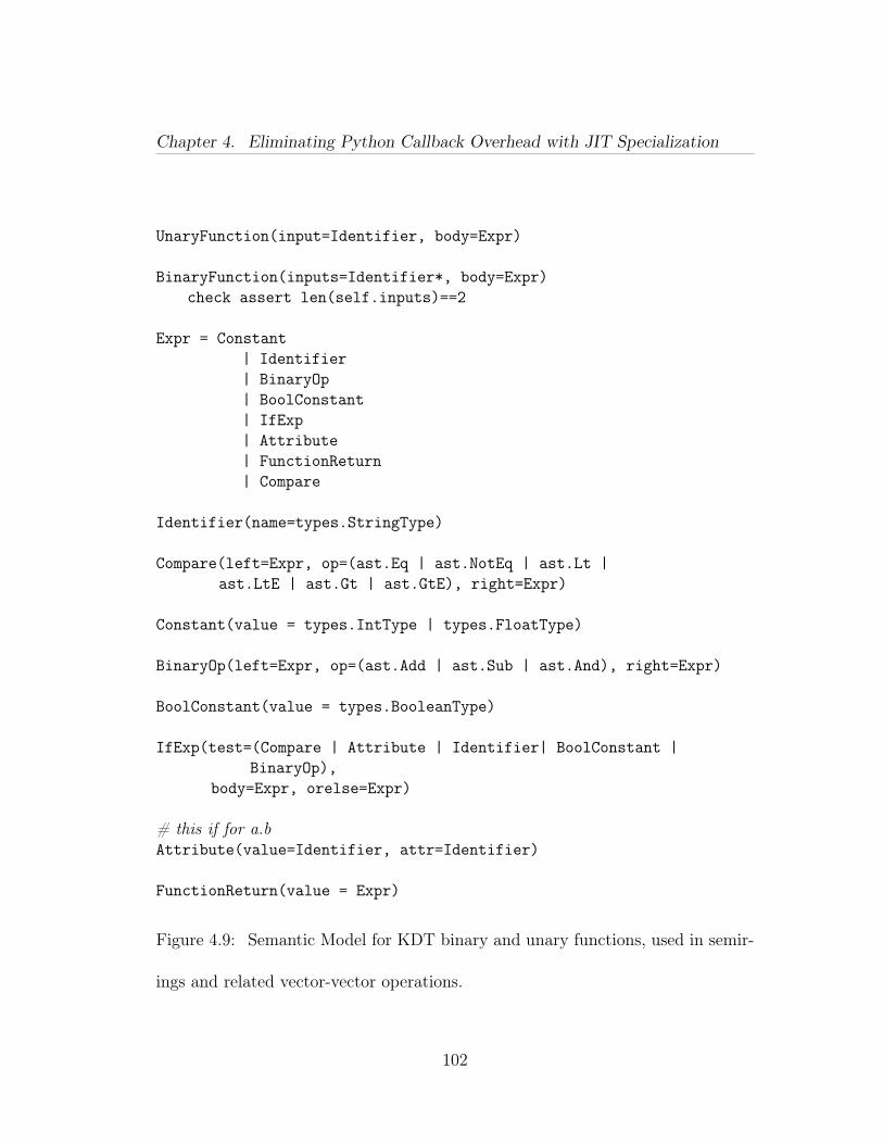
Chapter 4. Eliminating Python Callback Overhead with JIT Specialization
UnaryFunction(input=Identifier, body=Expr)
BinaryFunction(inputs=Identifier*, body=Expr)check assert len(self.inputs)==2
Expr = Constant| Identifier| BinaryOp| BoolConstant| IfExp| Attribute| FunctionReturn| Compare
Identifier(name=types.StringType)
Compare(left=Expr, op=(ast.Eq | ast.NotEq | ast.Lt |ast.LtE | ast.Gt | ast.GtE), right=Expr)
Constant(value = types.IntType | types.FloatType)
BinaryOp(left=Expr, op=(ast.Add | ast.Sub | ast.And), right=Expr)
BoolConstant(value = types.BooleanType)
IfExp(test=(Compare | Attribute | Identifier| BoolConstant |BinaryOp),
body=Expr, orelse=Expr)
# this if for a.bAttribute(value=Identifier, attr=Identifier)
FunctionReturn(value = Expr)
Figure 4.9: Semantic Model for KDT binary and unary functions, used in semir-
ings and related vector-vector operations.
102
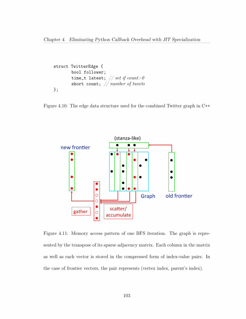
Chapter 4. Eliminating Python Callback Overhead with JIT Specialization
struct TwitterEdge {bool follower;time_t latest; // set if count>0short count; // number of tweets
};
Figure 4.10: The edge data structure used for the combined Twitter graph in C++
Graph&
gather& sca,er/&accumulate&
old&fron5er&
new&fron5er&
(stanza9like)&
Figure 4.11: Memory access pattern of one BFS iteration. The graph is repre-
sented by the transpose of its sparse adjacency matrix. Each column in the matrix
as well as each vector is stored in the compressed form of index-value pairs. In
the case of frontier vectors, the pair represents (vertex index, parent’s index).
103
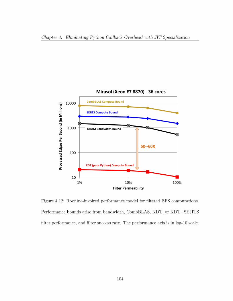
Chapter 4. Eliminating Python Callback Overhead with JIT Specialization
10#
100#
1000#
10000#
1%# 10%# 100%#
Processed(Ed
ges(P
er(Secon
d((in
(Millions)(
Filter(Permeability(
Mirasol((Xeon(E7(8870)(<(36(cores(
CombBLAS(Compute(Bound(
SEJITS(Compute(Bound(
DRAM(Bandwidth(Bound(
KDT((pure(Python)(Compute(Bound(
50<<60X(
Figure 4.12: Roofline-inspired performance model for filtered BFS computations.
Performance bounds arise from bandwidth, CombBLAS, KDT, or KDT+SEJITS
filter performance, and filter success rate. The performance axis is in log-10 scale.
104
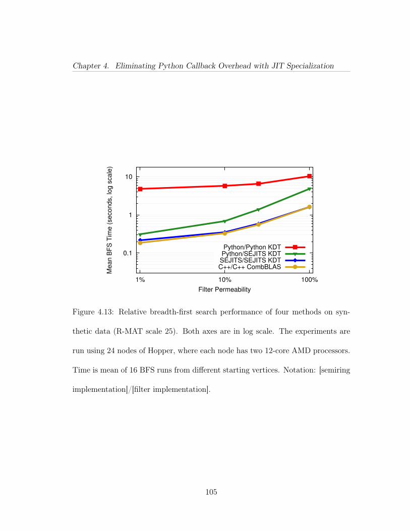
Chapter 4. Eliminating Python Callback Overhead with JIT Specialization
0.1
1
10
1% 10% 100%
Me
an
BF
S T
ime
(se
co
nd
s,
log
sca
le)
Filter Permeability
Python/Python KDTPython/SEJITS KDTSEJITS/SEJITS KDTC++/C++ CombBLAS
Figure 4.13: Relative breadth-first search performance of four methods on syn-
thetic data (R-MAT scale 25). Both axes are in log scale. The experiments are
run using 24 nodes of Hopper, where each node has two 12-core AMD processors.
Time is mean of 16 BFS runs from different starting vertices. Notation: [semiring
implementation]/[filter implementation].
105
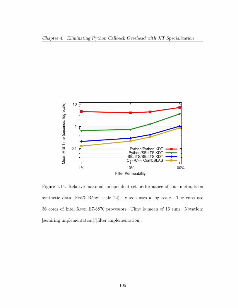
Chapter 4. Eliminating Python Callback Overhead with JIT Specialization
0.1
1
10
1% 10% 100%
Me
an
MIS
Tim
e (
se
co
nd
s,
log
sca
le)
Filter Permeability
Python/Python KDTPython/SEJITS KDTSEJITS/SEJITS KDTC++/C++ CombBLAS
Figure 4.14: Relative maximal independent set performance of four methods on
synthetic data (Erdős-Rényi scale 22). y-axis uses a log scale. The runs use
36 cores of Intel Xeon E7-8870 processors. Time is mean of 16 runs. Notation:
[semiring implementation]/[filter implementation].
106
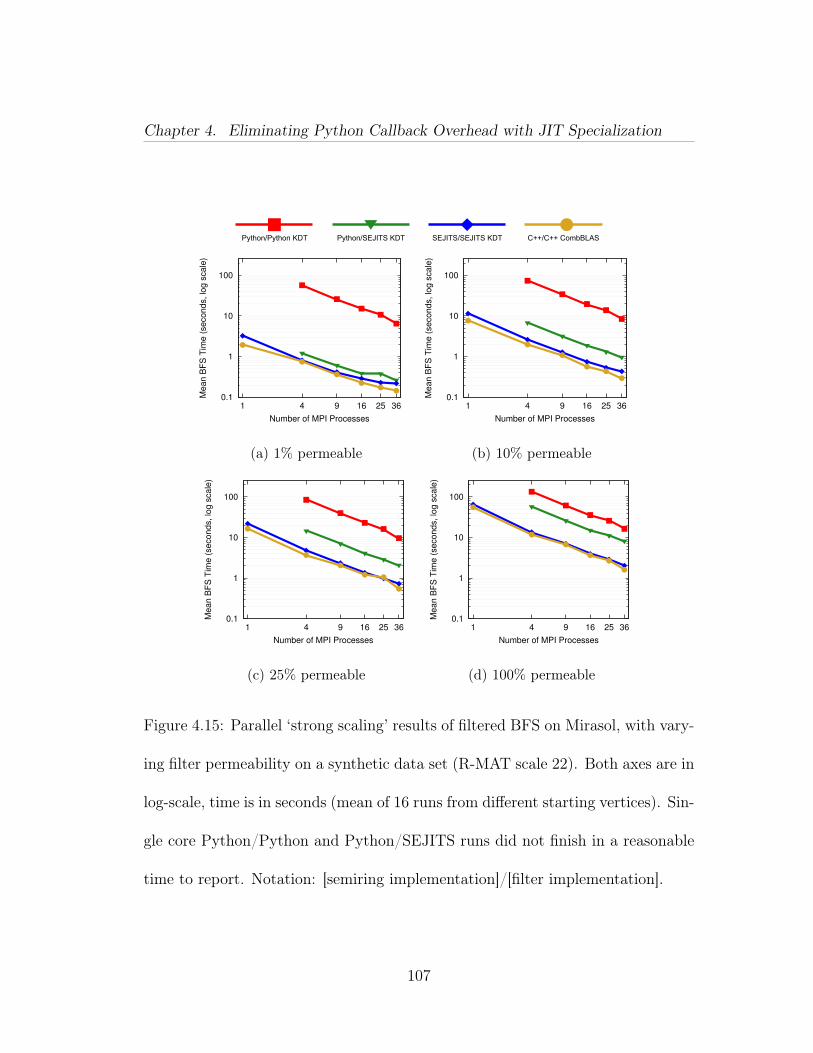
Chapter 4. Eliminating Python Callback Overhead with JIT Specialization
Python/Python KDT Python/SEJITS KDT SEJITS/SEJITS KDT C++/C++ CombBLAS
0.1
1
10
100
1 4 9 16 25 36
Mean B
FS
Tim
e (
seconds, lo
g s
cale
)
Number of MPI Processes
(a) 1% permeable
0.1
1
10
100
1 4 9 16 25 36
Mean B
FS
Tim
e (
seconds, lo
g s
cale
)Number of MPI Processes
(b) 10% permeable
0.1
1
10
100
1 4 9 16 25 36
Mean B
FS
Tim
e (
seconds, lo
g s
cale
)
Number of MPI Processes
(c) 25% permeable
0.1
1
10
100
1 4 9 16 25 36
Mean B
FS
Tim
e (
seconds, lo
g s
cale
)
Number of MPI Processes
(d) 100% permeable
Figure 4.15: Parallel ‘strong scaling’ results of filtered BFS on Mirasol, with vary-
ing filter permeability on a synthetic data set (R-MAT scale 22). Both axes are in
log-scale, time is in seconds (mean of 16 runs from different starting vertices). Sin-
gle core Python/Python and Python/SEJITS runs did not finish in a reasonable
time to report. Notation: [semiring implementation]/[filter implementation].
107
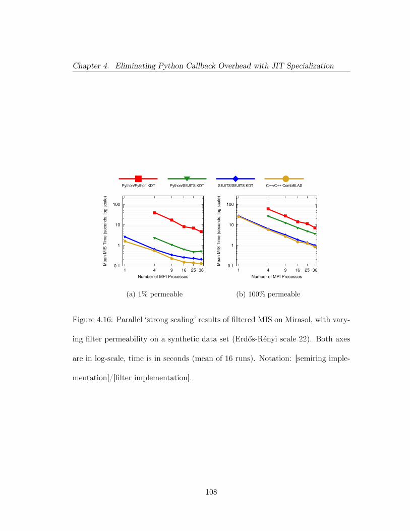
Chapter 4. Eliminating Python Callback Overhead with JIT Specialization
Python/Python KDT Python/SEJITS KDT SEJITS/SEJITS KDT C++/C++ CombBLAS
0.1
1
10
100
1 4 9 16 25 36
Mean M
IS T
ime (
seconds, lo
g s
cale
)
Number of MPI Processes
(a) 1% permeable
0.1
1
10
100
1 4 9 16 25 36
Mean M
IS T
ime (
seconds, lo
g s
cale
)
Number of MPI Processes
(b) 100% permeable
Figure 4.16: Parallel ‘strong scaling’ results of filtered MIS on Mirasol, with vary-
ing filter permeability on a synthetic data set (Erdős-Rényi scale 22). Both axes
are in log-scale, time is in seconds (mean of 16 runs). Notation: [semiring imple-
mentation]/[filter implementation].
108
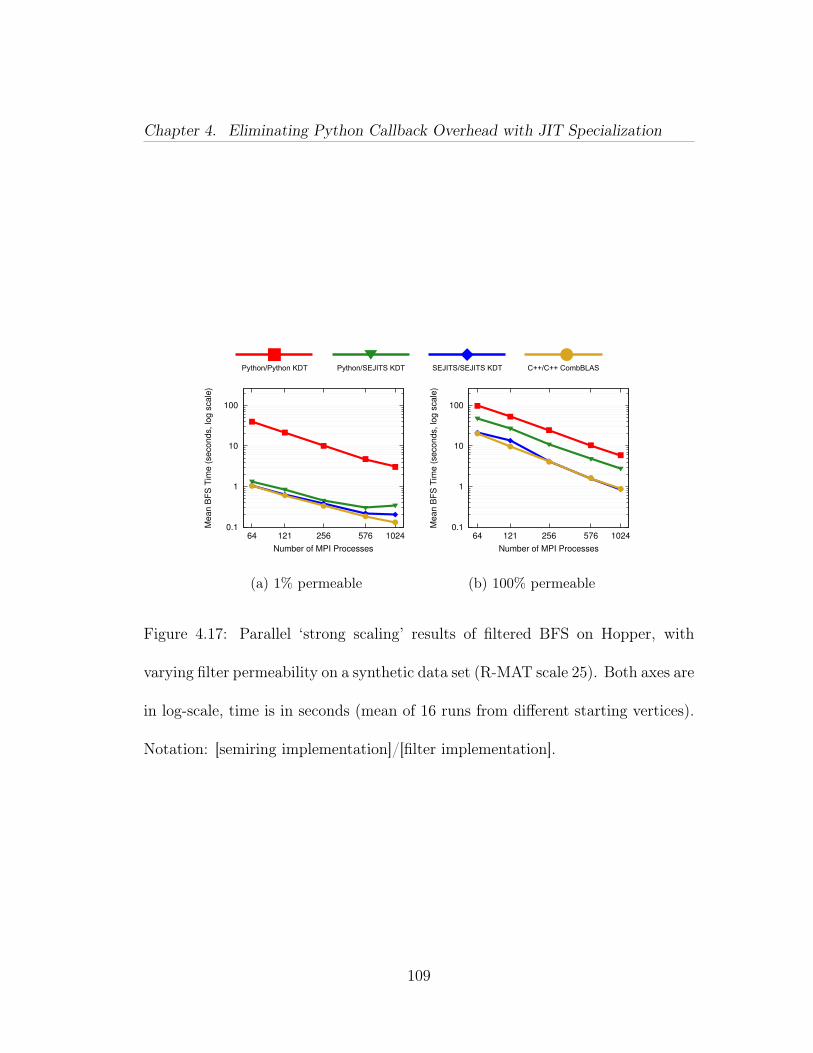
Chapter 4. Eliminating Python Callback Overhead with JIT Specialization
Python/Python KDT Python/SEJITS KDT SEJITS/SEJITS KDT C++/C++ CombBLAS
0.1
1
10
100
64 121 256 576 1024
Mean B
FS
Tim
e (
seconds, lo
g s
cale
)
Number of MPI Processes
(a) 1% permeable
0.1
1
10
100
64 121 256 576 1024
Mean B
FS
Tim
e (
seconds, lo
g s
cale
)
Number of MPI Processes
(b) 100% permeable
Figure 4.17: Parallel ‘strong scaling’ results of filtered BFS on Hopper, with
varying filter permeability on a synthetic data set (R-MAT scale 25). Both axes are
in log-scale, time is in seconds (mean of 16 runs from different starting vertices).
Notation: [semiring implementation]/[filter implementation].
109
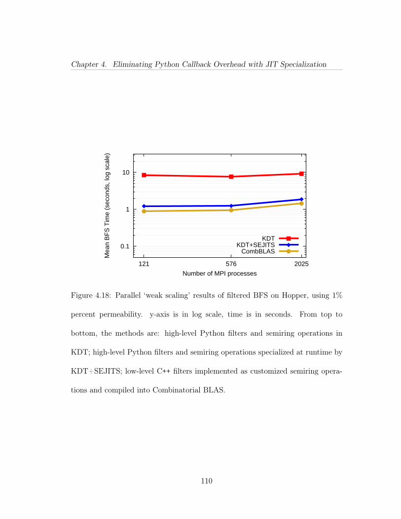
Chapter 4. Eliminating Python Callback Overhead with JIT Specialization
0.1
1
10
121 576 2025
Mea
n B
FS
Tim
e (s
econ
ds, l
og s
cale
)
Number of MPI processes
KDTKDT+SEJITS
CombBLAS
Figure 4.18: Parallel ‘weak scaling’ results of filtered BFS on Hopper, using 1%
percent permeability. y-axis is in log scale, time is in seconds. From top to
bottom, the methods are: high-level Python filters and semiring operations in
KDT; high-level Python filters and semiring operations specialized at runtime by
KDT+SEJITS; low-level C++ filters implemented as customized semiring opera-
tions and compiled into Combinatorial BLAS.
110
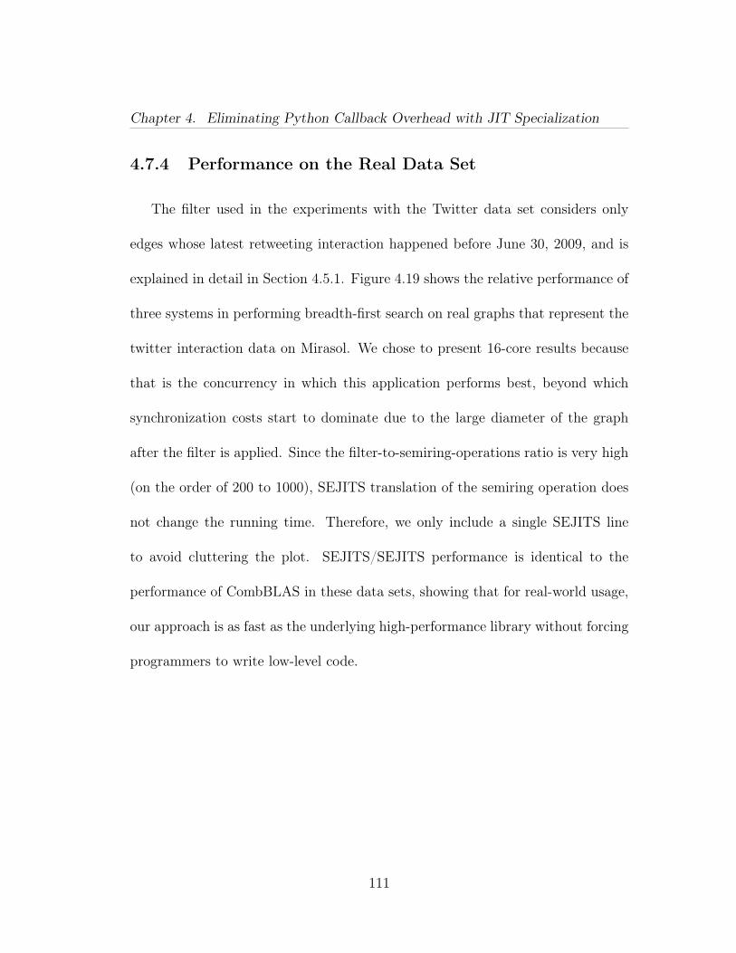
Chapter 4. Eliminating Python Callback Overhead with JIT Specialization
4.7.4 Performance on the Real Data Set
The filter used in the experiments with the Twitter data set considers only
edges whose latest retweeting interaction happened before June 30, 2009, and is
explained in detail in Section 4.5.1. Figure 4.19 shows the relative performance of
three systems in performing breadth-first search on real graphs that represent the
twitter interaction data on Mirasol. We chose to present 16-core results because
that is the concurrency in which this application performs best, beyond which
synchronization costs start to dominate due to the large diameter of the graph
after the filter is applied. Since the filter-to-semiring-operations ratio is very high
(on the order of 200 to 1000), SEJITS translation of the semiring operation does
not change the running time. Therefore, we only include a single SEJITS line
to avoid cluttering the plot. SEJITS/SEJITS performance is identical to the
performance of CombBLAS in these data sets, showing that for real-world usage,
our approach is as fast as the underlying high-performance library without forcing
programmers to write low-level code.
111
Chapter 4. Eliminating Python Callback Overhead with JIT Specialization
0.1
1
10
small medium large huge
Me
an
BF
S T
ime
(se
co
nd
s,
log
sca
le)
Twitter Input Graph
Python/Python KDTSEJITS/SEJITS KDTC++/C++ CombBLAS
Figure 4.19: Relative filtered breadth-first search performance of three methods
on real Twitter data. The y-axis is in seconds on a log scale. The runs use 16
cores of Intel Xeon E7-8870 processors.
112
Chapter 4. Eliminating Python Callback Overhead with JIT Specialization
4.8 Results From Hardware Performance Coun-
ters
The Performance Application Programming Interface (PAPI) library [4] pro-
vides direct access to low-level performance counters. These counters can measure
performance attributes of a particular program execution. For example, PAPI
counters can be used to measure the total number of instructions executed, or the
total number of cache misses (L1 or L2, data or instruction).
Our study incorporates several PAPI performance counters to gain a detailed
analysis of the performance benefits of KDT+SEJITS over Python KDT. We
are particularly interested in the PAPI_TOT_INS (total instructions completed),
PAPI_L1_ICM (number of L1 instruction cache misses), PAPI_L1_DCM (number of
L1 data cache misses), and PAPI_L2_TCM (number of L2 total cache misses). Ad-
ditional experiments with L3 cache misses did not provide any additional insights
that were not already captured in the L2 cache analysis.
Performance counters were examined for our breadth-first search program on
a scale 22 RMAT graph as described in Section 4.5, using both 10% and 100%
permeable on-the-fly filters, repeating a BFS from a single starting vertex 16 times.
These tests were conducted on Mirasol using 9 MPI processes, ensuring that all
processes are placed on a single socket. Note that each part of each BFS iteration
113
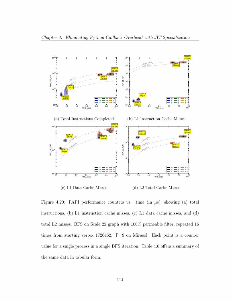
Chapter 4. Eliminating Python Callback Overhead with JIT Specialization
0.0 0.5 1.0 1.5 2.0 2.5 3.0TIME_usec 1e7
109
1010
1011
1012
PAPI_TOT_INS
IPC=2
.0
IPC=1
.0
IPC=0
.5
SpMV 3SEJITS
SpMV 4SEJITS
SpMV 4Python
SpMV 3Python
p 0
p 1
p 2
p 3
p 4
p 5
p 6
p 7
p 8
(a) Total Instructions Completed
0.0 0.5 1.0 1.5 2.0 2.5 3.0TIME_usec 1e7
104
105
106
107
108
109
1010
PAPI_L1
_ICM
5000 MB/s10000 MB/s
SpMV 3SEJITS
SpMV 4SEJITS
SpMV 4Python
SpMV 3Python
p 0
p 1
p 2
p 3
p 4
p 5
p 6
p 7
p 8
(b) L1 Instruction Cache Misses
0.0 0.5 1.0 1.5 2.0 2.5 3.0TIME_usec 1e7
107
108
109
PAPI_L1_D
CM
1000 MB/s
2000 MB/s
SpMV 3SEJITS
SpMV 4SEJITS
SpMV 4Python
SpMV 3Python
p 0
p 1
p 2
p 3
p 4
p 5
p 6
p 7
p 8
(c) L1 Data Cache Misses
0.0 0.5 1.0 1.5 2.0 2.5 3.0TIME_usec 1e7
106
107
108
109
PAPI_L2
_TCM
250 MB
/s500
MB/s
1000 M
B/s
SpMV 3SEJITS
SpMV 4SEJITS
SpMV 4Python
SpMV 3Python
p 0
p 1
p 2
p 3
p 4
p 5
p 6
p 7
p 8
(d) L2 Total Cache Misses
Figure 4.20: PAPI performance counters vs. time (in µs), showing (a) total
instructions, (b) L1 instruction cache misses, (c) L1 data cache misses, and (d)
total L2 misses. BFS on Scale 22 graph with 100% permeable filter, repeated 16
times from starting vertex 1726462. P=9 on Mirasol. Each point is a counter
value for a single process in a single BFS iteration. Table 4.6 offers a summary of
the same data in tabular form.
114
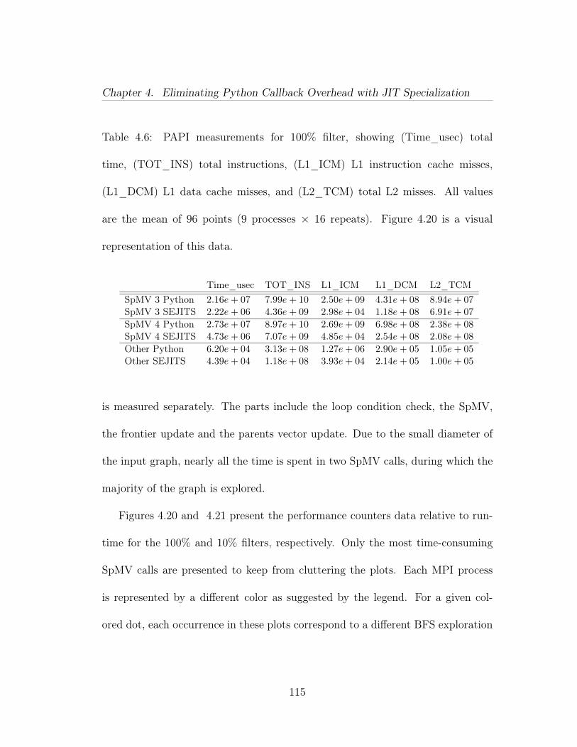
Chapter 4. Eliminating Python Callback Overhead with JIT Specialization
Table 4.6: PAPI measurements for 100% filter, showing (Time_usec) total
time, (TOT_INS) total instructions, (L1_ICM) L1 instruction cache misses,
(L1_DCM) L1 data cache misses, and (L2_TCM) total L2 misses. All values
are the mean of 96 points (9 processes × 16 repeats). Figure 4.20 is a visual
representation of this data.
Time_usec TOT_INS L1_ICM L1_DCM L2_TCMSpMV 3 Python 2.16e+ 07 7.99e+ 10 2.50e+ 09 4.31e+ 08 8.94e+ 07SpMV 3 SEJITS 2.22e+ 06 4.36e+ 09 2.98e+ 04 1.18e+ 08 6.91e+ 07
SpMV 4 Python 2.73e+ 07 8.97e+ 10 2.69e+ 09 6.98e+ 08 2.38e+ 08SpMV 4 SEJITS 4.73e+ 06 7.07e+ 09 4.85e+ 04 2.54e+ 08 2.08e+ 08
Other Python 6.20e+ 04 3.13e+ 08 1.27e+ 06 2.90e+ 05 1.05e+ 05Other SEJITS 4.39e+ 04 1.18e+ 08 3.93e+ 04 2.14e+ 05 1.00e+ 05
is measured separately. The parts include the loop condition check, the SpMV,
the frontier update and the parents vector update. Due to the small diameter of
the input graph, nearly all the time is spent in two SpMV calls, during which the
majority of the graph is explored.
Figures 4.20 and 4.21 present the performance counters data relative to run-
time for the 100% and 10% filters, respectively. Only the most time-consuming
SpMV calls are presented to keep from cluttering the plots. Each MPI process
is represented by a different color as suggested by the legend. For a given col-
ored dot, each occurrence in these plots correspond to a different BFS exploration
115
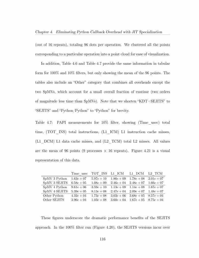
Chapter 4. Eliminating Python Callback Overhead with JIT Specialization
(out of 16 repeats), totaling 96 dots per operation. We clustered all the points
corresponding to a particular operation into a point cloud for ease of visualization.
In addition, Table 4.6 and Table 4.7 provide the same information in tabular
form for 100% and 10% filters, but only showing the mean of the 96 points. The
tables also include an “Other” category that combines all overheads except the
two SpMVs, which account for a small overall fraction of runtime (two orders
of magnitude less time than SpMVs). Note that we shorten “KDT+SEJITS” to
“SEJITS” and “Python/Python” to “Python” for brevity.
Table 4.7: PAPI measurements for 10% filter, showing (Time_usec) total
time, (TOT_INS) total instructions, (L1_ICM) L1 instruction cache misses,
(L1_DCM) L1 data cache misses, and (L2_TCM) total L2 misses. All values
are the mean of 96 points (9 processes × 16 repeats). Figure 4.21 is a visual
representation of this data.
Time_usec TOT_INS L1_ICM L1_DCM L2_TCMSpMV 3 Python 1.63e+ 07 5.97e+ 10 1.86e+ 09 1.78e+ 08 2.01e+ 07SpMV 3 SEJITS 6.58e+ 05 1.08e+ 09 2.46e+ 04 2.48e+ 07 1.66e+ 07
SpMV 4 Python 9.61e+ 06 3.59e+ 10 1.13e+ 09 1.14e+ 08 1.67e+ 07SpMV 4 SEJITS 5.39e+ 05 8.13e+ 08 2.47e+ 04 2.09e+ 07 1.48e+ 07
Other Python 4.32e+ 04 1.73e+ 08 3.03e+ 06 3.68e+ 05 8.57e+ 04Other SEJITS 3.96e+ 04 1.03e+ 08 3.60e+ 04 1.67e+ 05 8.75e+ 04
These figures underscore the dramatic performance benefits of the SEJITS
approach. In the 100% filter run (Figure 4.20), the SEJITS versions incur over
116
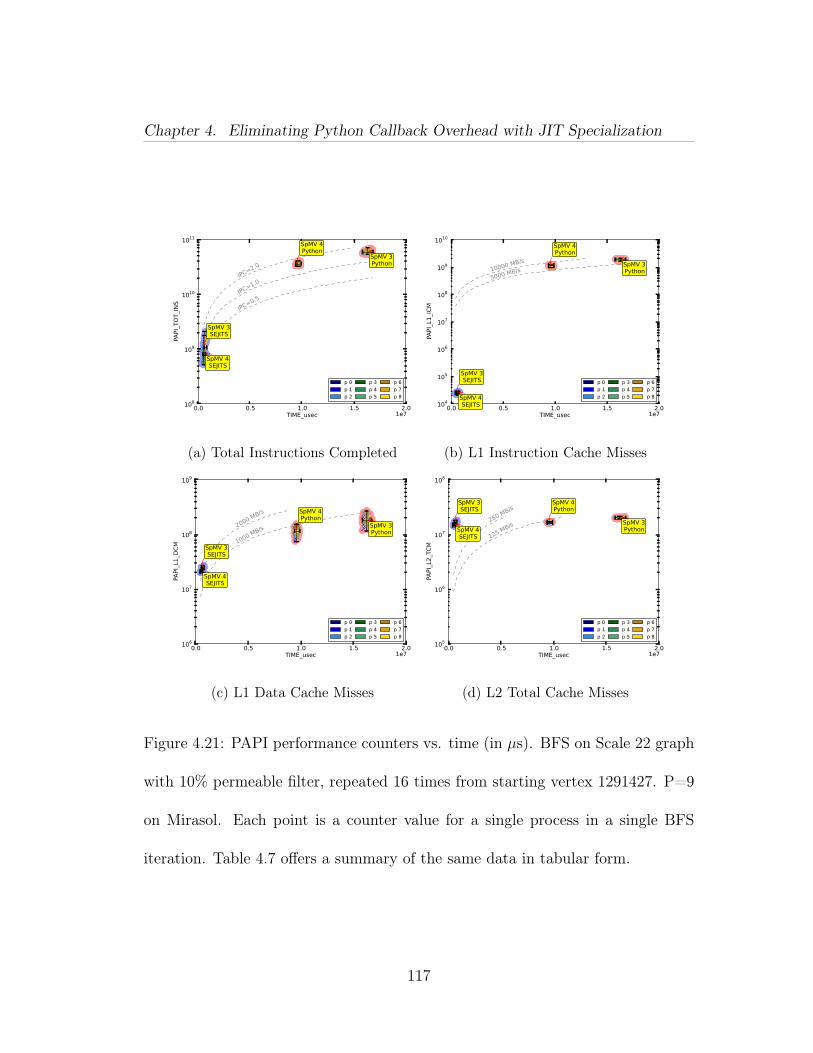
Chapter 4. Eliminating Python Callback Overhead with JIT Specialization
0.0 0.5 1.0 1.5 2.0TIME_usec 1e7
108
109
1010
1011
PAPI_TOT_INS
IPC=2
.0
IPC=1
.0
IPC=0
.5
SpMV 3SEJITS
SpMV 4SEJITS
SpMV 4Python
SpMV 3Python
p 0
p 1
p 2
p 3
p 4
p 5
p 6
p 7
p 8
(a) Total Instructions Completed
0.0 0.5 1.0 1.5 2.0TIME_usec 1e7
104
105
106
107
108
109
1010
PAPI_L1
_ICM
5000 MB/s10000 MB/s
SpMV 3SEJITS
SpMV 4SEJITS
SpMV 4Python
SpMV 3Python
p 0
p 1
p 2
p 3
p 4
p 5
p 6
p 7
p 8
(b) L1 Instruction Cache Misses
0.0 0.5 1.0 1.5 2.0TIME_usec 1e7
106
107
108
109
PAPI_L1_D
CM 10
00 MB
/s2000 MB
/s
SpMV 3SEJITS
SpMV 4SEJITS
SpMV 4Python
SpMV 3Python
p 0
p 1
p 2
p 3
p 4
p 5
p 6
p 7
p 8
(c) L1 Data Cache Misses
0.0 0.5 1.0 1.5 2.0TIME_usec 1e7
105
106
107
108
PAPI_
L2_T
CM
125 M
B/s25
0 MB/s
SpMV 3SEJITS
SpMV 4SEJITS
SpMV 4Python
SpMV 3Python
p 0
p 1
p 2
p 3
p 4
p 5
p 6
p 7
p 8
(d) L2 Total Cache Misses
Figure 4.21: PAPI performance counters vs. time (in µs). BFS on Scale 22 graph
with 10% permeable filter, repeated 16 times from starting vertex 1291427. P=9
on Mirasol. Each point is a counter value for a single process in a single BFS
iteration. Table 4.7 offers a summary of the same data in tabular form.
117
Chapter 4. Eliminating Python Callback Overhead with JIT Specialization
an order of magnitude fewer total instruction completions, as well as four orders
of magnitude fewer L1 instruction cache misses. The Python callbacks require a
wrapper object, while their SEJITS counterparts do not. This results in a further
half-order of magnitude fewer L1 data cache misses. The benefits are even larger
for the 10% filter run, as shown in Figure 4.21. The L2 total cache misses are
nearly same for both approaches, indicating that the majority of the performance
impact between SEJITS and pure Python approaches is captured within the L1
cache. This can be visually observed in the L2 total cache misses (d) plots,
where the SEJITS and Python clusters for SpMV 3 and SpMV 4 are on the same
horizontal line.
The only performance cost for SEJITS is the JIT compilation, incurred on
the first execution of a kernel which uses SEJITS callbacks. All our kernels use a
SEJITS callback, which amounts to about 20 seconds for just the first iteration.
Since the results of the JIT compilation are cached even between independent
jobs, this cost is only paid the first time the script is run.
118
Chapter 4. Eliminating Python Callback Overhead with JIT Specialization
4.9 Related Work
Graph Algorithm Packages
Pegasus [55] is a graph-analysis package that uses MapReduce [31] in a distributed-
computing setting. Other cloud-based graph analysis systems include GPS [94],
and Apache Hama [3], and Giraph [2]. Redekopp et al. [93] recently studied
performance optimizations for such cloud-based graph platforms.
Pegasus [55], uses a generalized matrix-vector multiplication primitive called
GIM-V, much like KDT’s SpMV, to express vertex-centered computations that com-
bine data from neighboring edges and vertices. In Pegasus, the semiring multiply
is referred to as combine2 and the semiring add is referred to as combineAll,
followed by an assign operation.
Powergraph [48] advocates a similar GAS (gather-apply-scatter) abstraction
for graph-parallel computations. This style of programming is called “think like
a vertex” in Pregel [78], a distributed-computing graph API. In traditional scien-
tific computing terminology, these are all BLAS-2 level operations; none of these
aforementioned systems currently include KDT’s BLAS-3 level SpGEMM “friends
of friends” primitive. BLAS-3 operations are higher level primitives that enable
more optimizations and generally deliver superior performance. Both Pegasus and
119
Chapter 4. Eliminating Python Callback Overhead with JIT Specialization
Powergraph require the application to be written in a relative low-level language
(Java and C++, respectively) and neither supports filtering.
Other libraries for high-performance computation on large-scale graphs include
the Parallel Boost Graph Library (PBGL) [50], the Combinatorial BLAS [24],
Georgia Tech’s SNAP [11], and the Multithreaded Graph Library (MTGL) [14].
These are all written in C/C++ and with the exception of the PBGL and MTGL
do not include explicit filter support. The first two support distributed memory
as well as shared memory while the latter two require a shared address space.
PBGL and MTGL provides generic filter support via visitor functions. PBGL
also supports an explicit FilteredGraph concept. Since PBGL and MTGL are
written in C++ with heavy use of template mechanisms, they are not conceptually
simple to use by domain scientists. By contrast, our approach targets usability
by specializing algorithms from a high-productivity language.
SPARQL [91] is a query language for Resource Description Framework (RDF) [61],
which supports semantic graph database queries. The existing database engines
that implement SPARQL and RDF handle filtering based queries efficiently but
they are not as effective for running traversal based tightly-coupled graph com-
putations scalably in parallel environments.
The closest previous work is Green Marl [53], a domain specific language (DSL)
for small-world graph exploration that runs on GPUs and multicore CPUs with-
120
Chapter 4. Eliminating Python Callback Overhead with JIT Specialization
out support for distributed machines (though such support is planned). Green
Marl supports a very different programming model than KDT. In Green Marl,
programmers iterate over nodes/edges or access them in specific traversal orders;
work can be accomplished within a traversal or iteration step. KDT’s under-
lying linear algebra abstraction allows graph algorithms to be implemented by
customizing generic high-performance primitives of CombBLAS. In addition, the
approach of Green Marl is to use an external DSL that has a different syntax and
compiler than the rest of an application; KDT allows users to write their entire
application in Python.
JIT Compilation of DSLs
Embedded DSLs [38] for domain-specific computations have a rich history,
including DSLs that are compiled instead of interpreted [65]. Abstract Syntax
Tree introspection for such DSLs has been used most prominently for database
queries in ActiveRecord [1], part of the Ruby on Rails framework.
The approach applied here, which uses AST introspection combined with tem-
plates, was first applied to stencil algorithms and data parallel constructs [27],
and subsequently to a number of domains including linear algebra and Gaussian
mixture modeling [54].
121
Chapter 4. Eliminating Python Callback Overhead with JIT Specialization
Finally, general JIT approaches for Python such as PyPy [5] do not offer the
advantages of embedded DSLs such as domain-specific optimizations and the lack
of need to perform detailed domain analysis.
4.10 Conclusion
The KDT graph analytics system achieves customizability through user-defined
filters, high performance through the use of a scalable parallel library, and concep-
tual simplicity through appropriate graph abstractions expressed in a high-level
language.
We have shown that the performance impact of expressing filters in a high-
level language like Python can be mitigated by Selective Embedded Just-in-Time
Specialization. In particular, we have shown that our embedded DSLs for filters
and semirings enable Python code to achieve comparable performance to a pure
C++ implementation. In addition, we provide users with the ability to define
new vertex and edge types from Python, yet still obtain the same high perfor-
mance. A Roofline analysis shows that specialization enables filtering to move
from being compute-bound to memory-bandwidth-bound. Further performance-
counter-based analysis shows that the SEJITS performance gains are due to a
combination of executing fewer instructions and the ability to avoid data move-
122
Chapter 4. Eliminating Python Callback Overhead with JIT Specialization
ment for object wrappers during computation. We demonstrated our approach on
both real-world data and large synthetic datasets. Our approach scales to graphs
on the order of hundreds of millions of edges, and to machines with thousands of
processors, suggesting that our methodology can be applied to even more com-
putationally intensive graph analysis tasks in the future. Ultimately, the ability
to both attain high performance and scale to thousands of cores for most cases
makes it possible for domain scientists to efficiently utilize large-scale clusters and
supercomputers.
In future work we will further generalize our DSL to support a larger subset of
Python, as well as expanding SEJITS support beyond filtering and semiring op-
erations to cover more KDT primitives. An open question is whether CombBLAS
performance can be pushed closer to the bandwidth limit by eliminating internal
data structure overheads.
123
Chapter 5
Shared Memory SparseMatrix-Sparse MatrixMultiplication
This chapter is based on a technical report [75] and an extended abstract
published in CSC’14 [76].
5.1 Introduction
Sparse matrix-matrix multiplication (or SpGEMM ) is a key primitive in some
graph algorithms (using various semirings) [57] and in numeric problems such
as algebraic multigrid [98]. Multicore shared memory systems can solve very
large problems [99], or can be part of a hybrid shared/distributed memory high-
performance architecture.
124
Chapter 5. Shared Memory Sparse Matrix-Sparse Matrix Multiplication
Two-dimensional decompositions are broadly used in state-of-the-art methods
for both dense [104] and sparse [22, 24] matrices. Quadtree matrix decompositions
and algorithms have a long history [40, 41, 95, 109, 110], including recursive matrix
multiplication [108].
In this chapter we describe a new sparse matrix data structure and the first
highly-parallel sparse matrix-matrix multiplication algorithm designed specifically
for shared memory.
5.2 Quadtree Representation
Our basic data structure is a 2D quadtree matrix decomposition. Unlike pre-
vious work that continues the quadtree until elements become leaves, we instead
terminate the quadtree early and store the elements in large leaf blocks. This
arrangement brings the best of both worlds; the quadtree provides isolation and
chunking, and the large leaf blocks provide locality and a way to amortize tree
costs.
There are many answers to the question of when to stop subdivision. We use
a simple strategy: subdivide until either leaf nnz or leaf size in bytes is below a
threshold. This threshold can be fixed or dynamically chosen to provide sufficient
parallelism for a particular matrix on a particular machine. The former approach
125
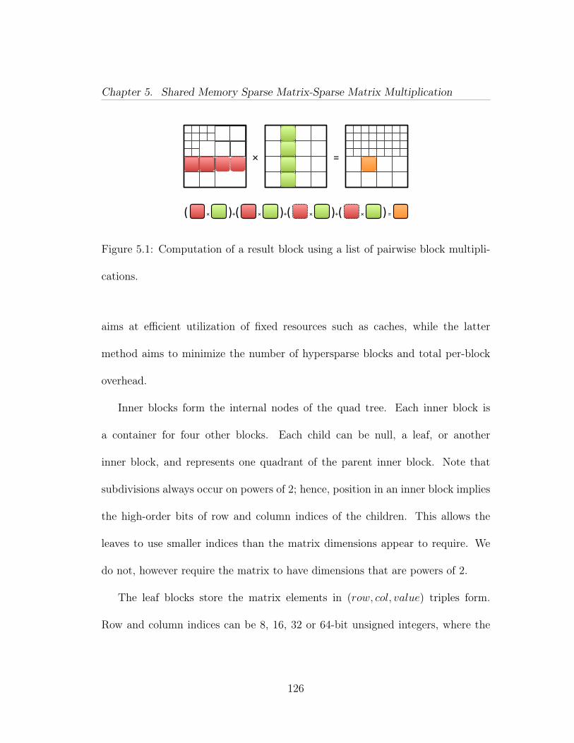
Chapter 5. Shared Memory Sparse Matrix-Sparse Matrix Multiplication
× =
× )+( ) = × × × ( )+( )+(
Figure 5.1: Computation of a result block using a list of pairwise block multipli-
cations.
aims at efficient utilization of fixed resources such as caches, while the latter
method aims to minimize the number of hypersparse blocks and total per-block
overhead.
Inner blocks form the internal nodes of the quad tree. Each inner block is
a container for four other blocks. Each child can be null, a leaf, or another
inner block, and represents one quadrant of the parent inner block. Note that
subdivisions always occur on powers of 2; hence, position in an inner block implies
the high-order bits of row and column indices of the children. This allows the
leaves to use smaller indices than the matrix dimensions appear to require. We
do not, however require the matrix to have dimensions that are powers of 2.
The leaf blocks store the matrix elements in (row, col, value) triples form.
Row and column indices can be 8, 16, 32 or 64-bit unsigned integers, where the
126
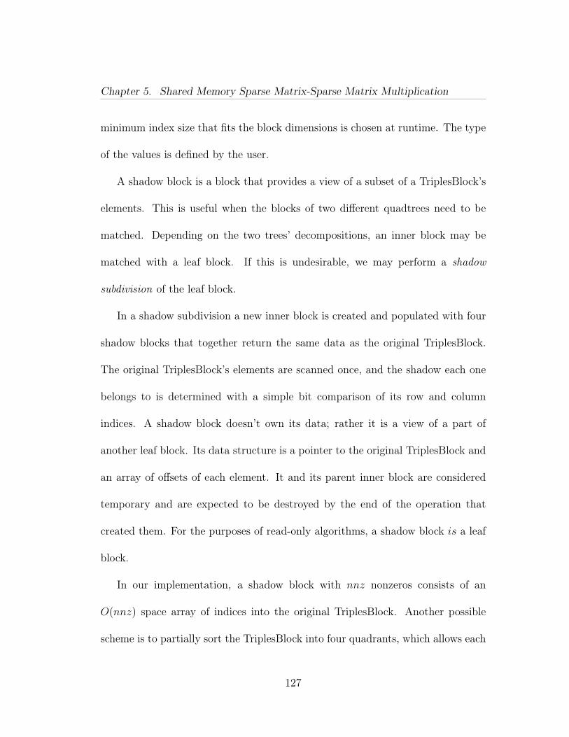
Chapter 5. Shared Memory Sparse Matrix-Sparse Matrix Multiplication
minimum index size that fits the block dimensions is chosen at runtime. The type
of the values is defined by the user.
A shadow block is a block that provides a view of a subset of a TriplesBlock’s
elements. This is useful when the blocks of two different quadtrees need to be
matched. Depending on the two trees’ decompositions, an inner block may be
matched with a leaf block. If this is undesirable, we may perform a shadow
subdivision of the leaf block.
In a shadow subdivision a new inner block is created and populated with four
shadow blocks that together return the same data as the original TriplesBlock.
The original TriplesBlock’s elements are scanned once, and the shadow each one
belongs to is determined with a simple bit comparison of its row and column
indices. A shadow block doesn’t own its data; rather it is a view of a part of
another leaf block. Its data structure is a pointer to the original TriplesBlock and
an array of offsets of each element. It and its parent inner block are considered
temporary and are expected to be destroyed by the end of the operation that
created them. For the purposes of read-only algorithms, a shadow block is a leaf
block.
In our implementation, a shadow block with nnz nonzeros consists of an
O(nnz) space array of indices into the original TriplesBlock. Another possible
scheme is to partially sort the TriplesBlock into four quadrants, which allows each
127
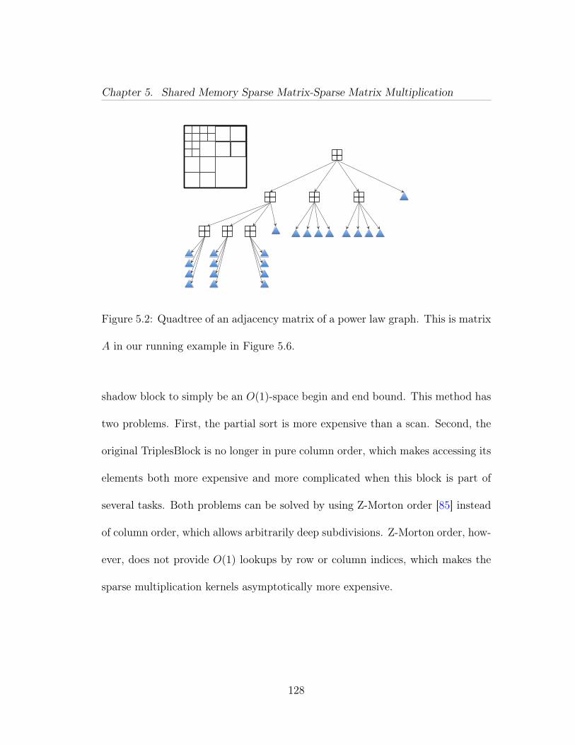
Chapter 5. Shared Memory Sparse Matrix-Sparse Matrix Multiplication
Figure 5.2: Quadtree of an adjacency matrix of a power law graph. This is matrix
A in our running example in Figure 5.6.
shadow block to simply be an O(1)-space begin and end bound. This method has
two problems. First, the partial sort is more expensive than a scan. Second, the
original TriplesBlock is no longer in pure column order, which makes accessing its
elements both more expensive and more complicated when this block is part of
several tasks. Both problems can be solved by using Z-Morton order [85] instead
of column order, which allows arbitrarily deep subdivisions. Z-Morton order, how-
ever, does not provide O(1) lookups by row or column indices, which makes the
sparse multiplication kernels asymptotically more expensive.
128
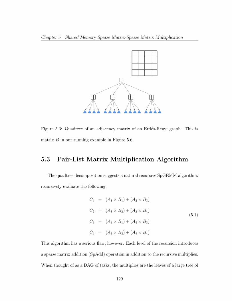
Chapter 5. Shared Memory Sparse Matrix-Sparse Matrix Multiplication
Figure 5.3: Quadtree of an adjacency matrix of an Erdős-Rényi graph. This is
matrix B in our running example in Figure 5.6.
5.3 Pair-List Matrix Multiplication Algorithm
The quadtree decomposition suggests a natural recursive SpGEMM algorithm:
recursively evaluate the following:
C4 = (A1 ×B1) + (A2 ×B3)
C2 = (A1 ×B2) + (A2 ×B4)
C3 = (A3 ×B1) + (A4 ×B3)
C4 = (A3 ×B2) + (A4 ×B4)
(5.1)
This algorithm has a serious flaw, however. Each level of the recursion introduces
a sparse matrix addition (SpAdd) operation in addition to the recursive multiplies.
When thought of as a DAG of tasks, the multiplies are the leaves of a large tree of
129
Chapter 5. Shared Memory Sparse Matrix-Sparse Matrix Multiplication
SpAdds. The number of SpAdds each block is involved in is equal to its depth in
the tree. Unfortunately, there is no known method to perform an SpAdd in time
proportional to only the FLOPs required. Instead, the total time of all additions
is proportional to total FLOPs plus the size of the operands times the height of
the tree. The add tree therefore imposes an unwanted log factor and becomes a
significant bottleneck. Our algorithm reformulates the operations such that the
SpAdds can be inlined into the leaf multiplies.
The algorithm consists of a symbolic phase and a computational phase. The
symbolic phase generates an execution strategy, and the computational phase
carries out that strategy. Each phase is itself a set of parallel tasks. We are
willing to temporarily reorganize data on-the-fly, and discard the changes after
use. This extra work does not add to the asymptotic complexity.
The source of parallelism of both phases comes from the recursive structure of
the quadtree of C. Each internal node yields a symbolic phase task, and each leaf
yields a computational phase task.
We choose to formulate a DAG of tasks and let a scheduling framework map
those tasks to threads. Our algorithm does not perform scheduling; rather, we
use a standard scheduling framework such as TBB, Cilk, or OpenMP.
130
Chapter 5. Shared Memory Sparse Matrix-Sparse Matrix Multiplication
5.3.1 Symbolic Phase
The symbolic phase divides computation of C = A×B into compute tasks such
that each compute task owns (is the only writer to) a particular block of C and
is supplied with a list of all the operands it needs to perform the multiplication.
Let Cown be a leaf block in C, and pairlist be the list of pairs of leaf blocks
from A and B whose block inner product is Cown:
Cown =∑|pairlist|
i=1Ai ×Bi (5.2)
The blocks Ai and Bi may be original leaf blocks or shadow blocks. The sym-
bolic phase recursively determines all the Cown and corresponding pairlist. Equa-
tion (5.2) still contains additions, but in Section 5.3.3 we describe a method to
evaluate (5.2) without explicit SpAdd steps.
To provide intuition for what we wish to accomplish, consider a dense β × β
grid of blocks instead of a quadtree. The result matrix will contain β2 blocks,
each one the result of a block inner product between the corresponding block row
of A and block column of B. The ith block in the block row of A is matched with
the ith block in the block column of B in this block inner product. Therefore,
we describe this block inner product with a list, named pairlist, with length β of
pairs of blocks.
131
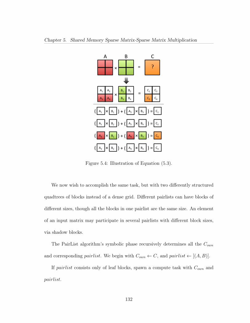
Chapter 5. Shared Memory Sparse Matrix-Sparse Matrix Multiplication
= C1 C2
C3 C4
A1 A2
A3 A4 ×
B1 B2
B3 B4
× =
B A C
C4 × ) + ( ) = × ( B4 A4 B2 A3
C1 × ) + ( ) = × ( B3 A2 B1 A1
C2 × ) + ( ) = × ( B4 A2 B2 A1
C3 × ) + ( ) = × ( B3 A4 B1 A3
?
Figure 5.4: Illustration of Equation (5.3).
We now wish to accomplish the same task, but with two differently structured
quadtrees of blocks instead of a dense grid. Different pairlists can have blocks of
different sizes, though all the blocks in one pairlist are the same size. An element
of an input matrix may participate in several pairlists with different block sizes,
via shadow blocks.
The PairList algorithm’s symbolic phase recursively determines all the Cown
and corresponding pairlist. We begin with Cown ← C, and pairlist← [(A,B)].
If pairlist consists only of leaf blocks, spawn a compute task with Cown and
pairlist.
132
Chapter 5. Shared Memory Sparse Matrix-Sparse Matrix Multiplication
If all the blocks in pairlist are divided, we divide Cown into four children with
one quadrant each and recurse, rephrasing divided C = A×B using (5.2):
C1 = [(A1, B1), (A2, B3)]
C2 = [(A1, B2), (A2, B4)]
C3 = [(A3, B1), (A4, B3)]
C4 = [(A3, B2), (A4, B4)]
(5.3)
In total, each recursive call receives a Cown and an entire list of pairs of blocks.
For every pair in pairlist, insert two pairs into each child’s pairlist according to
the respective line in (5.3). Each child’s pairlist is twice as long as the parent’s
pairlist, but totals only 4 sub-blocks to the parent’s 8.
If pairlist includes both divided blocks and leaf blocks, we temporarily divide
the leaves until all blocks in pairlist are equally divided. This temporary division
creates shadow blocks as described in Section 5.2. Shadow subdivision resolves any
differences in quadtree depth between the operands. It allows the symbolic phase
to recurse until only leaves remain, which lets the compute phase only operate on
leaves. See Figure 5.5 for an example. The shadow blocks persist only until the
end of the SpGEMM.
133
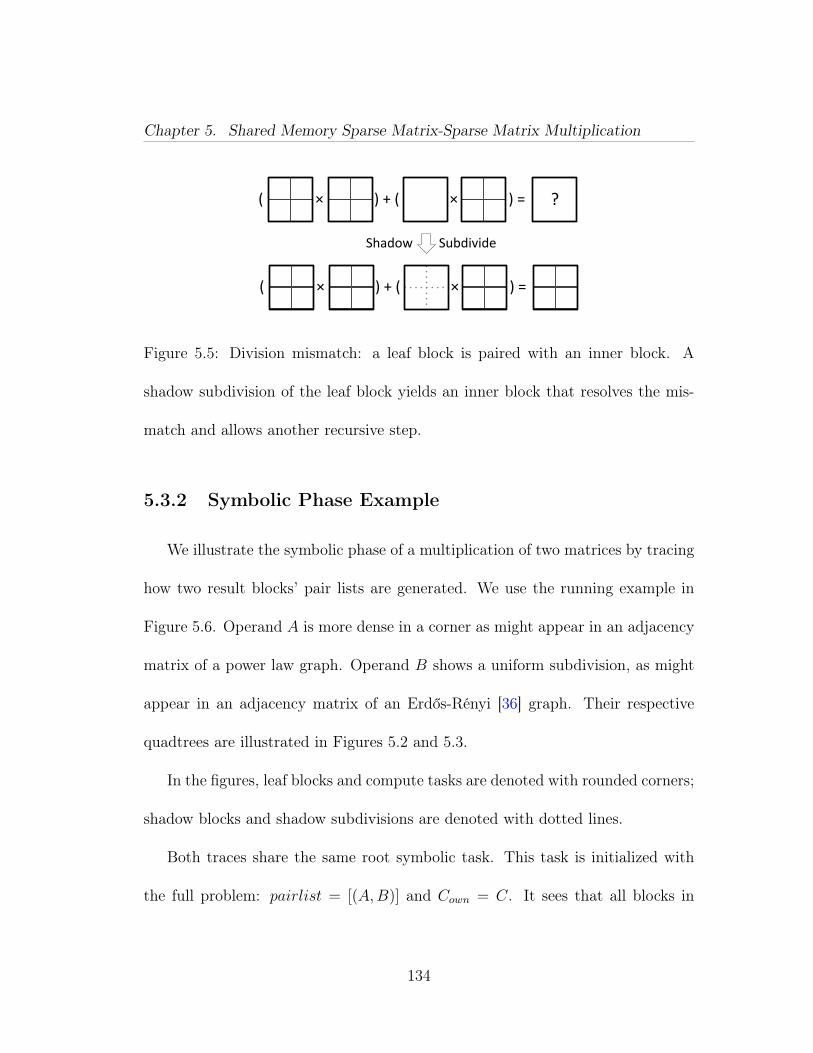
Chapter 5. Shared Memory Sparse Matrix-Sparse Matrix Multiplication
?
Shadow Subdivide
× ) + ( ) = × (
× ) + ( ) = × (
Figure 5.5: Division mismatch: a leaf block is paired with an inner block. A
shadow subdivision of the leaf block yields an inner block that resolves the mis-
match and allows another recursive step.
5.3.2 Symbolic Phase Example
We illustrate the symbolic phase of a multiplication of two matrices by tracing
how two result blocks’ pair lists are generated. We use the running example in
Figure 5.6. Operand A is more dense in a corner as might appear in an adjacency
matrix of a power law graph. Operand B shows a uniform subdivision, as might
appear in an adjacency matrix of an Erdős-Rényi [36] graph. Their respective
quadtrees are illustrated in Figures 5.2 and 5.3.
In the figures, leaf blocks and compute tasks are denoted with rounded corners;
shadow blocks and shadow subdivisions are denoted with dotted lines.
Both traces share the same root symbolic task. This task is initialized with
the full problem: pairlist = [(A,B)] and Cown = C. It sees that all blocks in
134
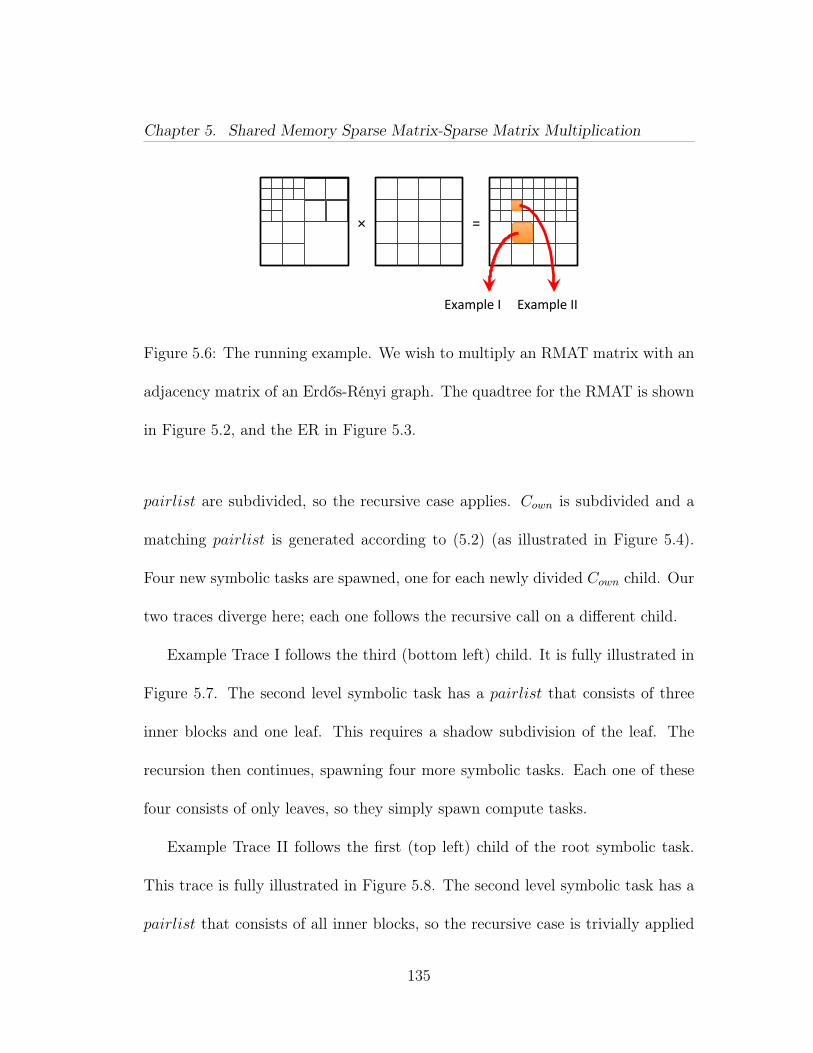
Chapter 5. Shared Memory Sparse Matrix-Sparse Matrix Multiplication
× =
Example II Example I
Figure 5.6: The running example. We wish to multiply an RMAT matrix with an
adjacency matrix of an Erdős-Rényi graph. The quadtree for the RMAT is shown
in Figure 5.2, and the ER in Figure 5.3.
pairlist are subdivided, so the recursive case applies. Cown is subdivided and a
matching pairlist is generated according to (5.2) (as illustrated in Figure 5.4).
Four new symbolic tasks are spawned, one for each newly divided Cown child. Our
two traces diverge here; each one follows the recursive call on a different child.
Example Trace I follows the third (bottom left) child. It is fully illustrated in
Figure 5.7. The second level symbolic task has a pairlist that consists of three
inner blocks and one leaf. This requires a shadow subdivision of the leaf. The
recursion then continues, spawning four more symbolic tasks. Each one of these
four consists of only leaves, so they simply spawn compute tasks.
Example Trace II follows the first (top left) child of the root symbolic task.
This trace is fully illustrated in Figure 5.8. The second level symbolic task has a
pairlist that consists of all inner blocks, so the recursive case is trivially applied
135
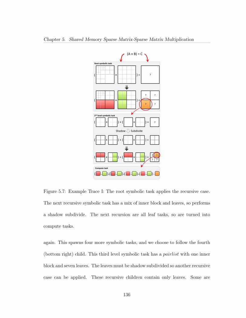
Chapter 5. Shared Memory Sparse Matrix-Sparse Matrix Multiplication
(A × B) = C
Compute task
× ) + ( ) = × (
× ) + ( ) = × ( ?
2nd level symbolic task
? ?
? ?
× ) = ?
? ?
× ) =
Root symbolic task
(
(
?
?
Shadow Subdivide
× ) + ( ) = × (
× )+( ) = × × × ( )+( )+(
Figure 5.7: Example Trace I: The root symbolic task applies the recursive case.
The next recursive symbolic task has a mix of inner block and leaves, so performs
a shadow subdivide. The next recursion are all leaf tasks, so are turned into
compute tasks.
again. This spawns four more symbolic tasks, and we choose to follow the fourth
(bottom right) child. This third level symbolic task has a pairlist with one inner
block and seven leaves. The leaves must be shadow subdivided so another recursive
case can be applied. These recursive children contain only leaves. Some are
136
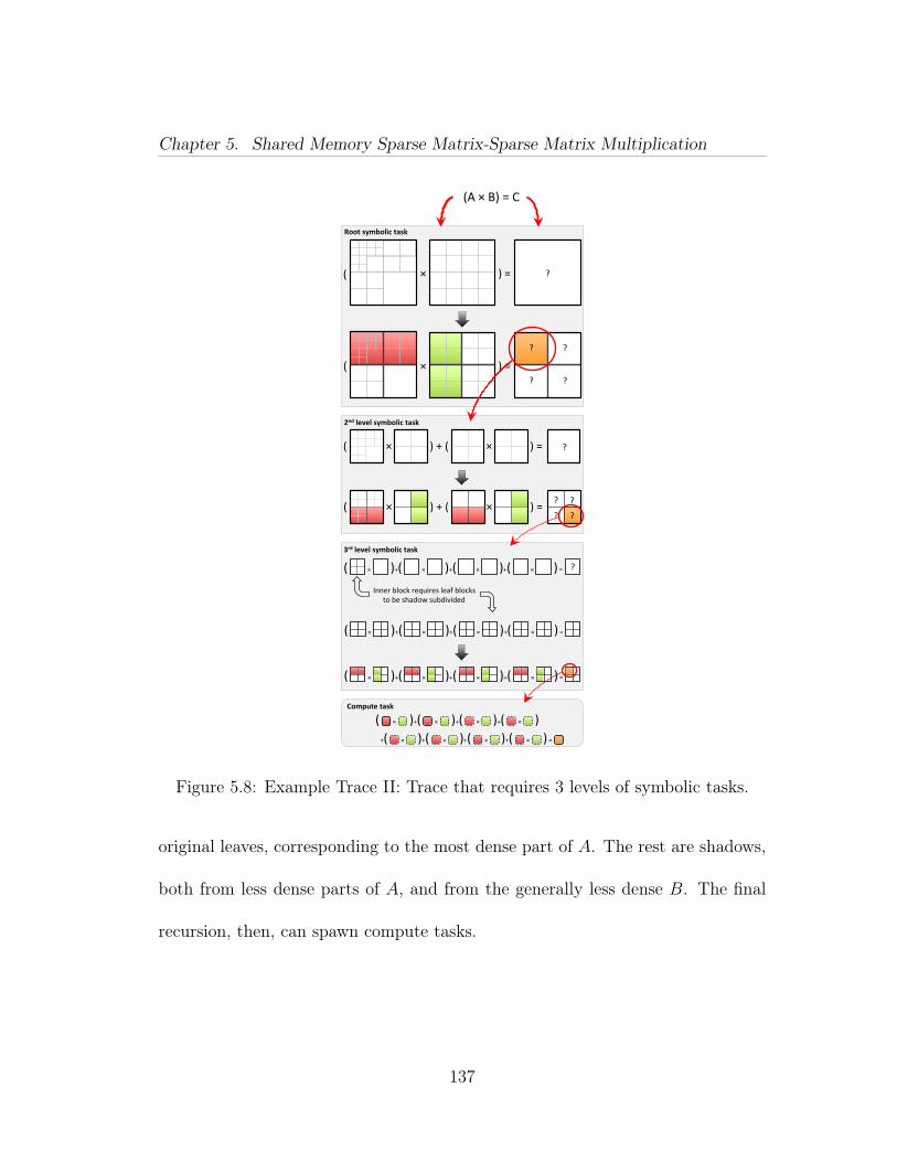
Chapter 5. Shared Memory Sparse Matrix-Sparse Matrix Multiplication
(A × B) = C
× )+( ) × × × ( )+( )+( × )+( ) = × × × )+( )+( +(
Compute task
× )+( ) = × × × ( )+( )+( Inner block requires leaf blocks
to be shadow subdivided
× )+( ) = × × × ( )+( )+(
?
× )+( ) = × × × ( )+( )+(
3rd level symbolic task
× ) + ( ) = × ( ?
2nd level symbolic task
× ) = ?
? ?
× ) =
Root symbolic task
(
(
?
?
× ) + ( ) = × ( ? ?
? ?
Figure 5.8: Example Trace II: Trace that requires 3 levels of symbolic tasks.
original leaves, corresponding to the most dense part of A. The rest are shadows,
both from less dense parts of A, and from the generally less dense B. The final
recursion, then, can spawn compute tasks.
137
Chapter 5. Shared Memory Sparse Matrix-Sparse Matrix Multiplication
5.3.3 Computational Phase
This phase consists of tasks that each compute one block inner product (5.2).
We present the final approach in Algorithm 2 and describe it below. Observe that
each compute task is lock-free because it only reads from the blocks in pairlist
and only writes to Cown.
We extend Gustavson’s sequential sparse matrix multiplication algorithm [51].
Gustavson computes the product of column j of B and A using a “sparse accu-
mulator”, or SPA. The SPA can be thought of as a dense auxiliary vector, or hash
map, that efficiently accumulates sparse updates to a single column of Cown. Gus-
tavson’s algorithm reads both A and B column-by-column, but their columns are
selected differently. The algorithm reads the non-empty columns of B in order,
but performs random lookups of columns in A. To facilitate these access patterns
for our (row, col, value) triples storage, we organize the column-sorted triples. A
column organizer is an auxiliary structure that allows quick access to particular
columns of a block. Due to different access patterns for blocks A and B, we
organize them differently.
138
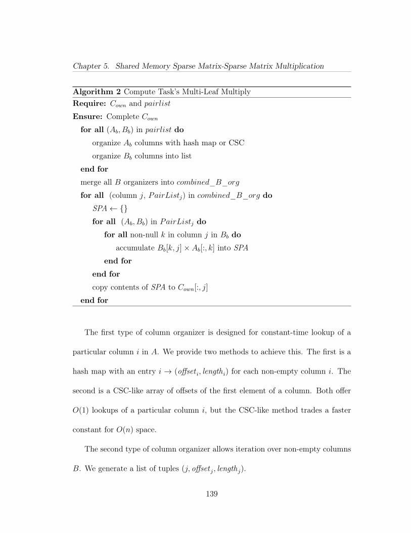
Chapter 5. Shared Memory Sparse Matrix-Sparse Matrix Multiplication
Algorithm 2 Compute Task’s Multi-Leaf MultiplyRequire: Cown and pairlist
Ensure: Complete Cown
for all (Ab, Bb) in pairlist do
organize Ab columns with hash map or CSC
organize Bb columns into list
end for
merge all B organizers into combined_B_org
for all (column j, PairListj) in combined_B_org do
SPA← {}for all (Ab, Bb) in PairListj do
for all non-null k in column j in Bb do
accumulate Bb[k, j]× Ab[:, k] into SPA
end for
end for
copy contents of SPA to Cown[:, j]
end for
The first type of column organizer is designed for constant-time lookup of a
particular column i in A. We provide two methods to achieve this. The first is a
hash map with an entry i → (offset i, length i) for each non-empty column i. The
second is a CSC-like array of offsets of the first element of a column. Both offer
O(1) lookups of a particular column i, but the CSC-like method trades a faster
constant for O(n) space.
The second type of column organizer allows iteration over non-empty columns
B. We generate a list of tuples (j, offset j, lengthj).
139
Chapter 5. Shared Memory Sparse Matrix-Sparse Matrix Multiplication
All column organizers are generated with a single scan of only the column
indices. Therefore each one takes linear time to generate. For maximum paral-
lelism, the organizers can be generated in each compute task. This means each
block is organized many times, once by each compute task it is used in. This cost
is negligible for small to medium matrices, but can be greatly reduced by caching
the organizers.
The column organizers allow us to efficiently use Gustavson’s algorithm on
our triples to evaluate the multiplies in (5.2). We show that if all pairwise block
multiplies in a computational task are performed simultaneously then they can
be interleaved in such a fashion that the addition step is inlined into the multiply
step.
The key to this inlining is the SPA. Gustavson uses the SPA to accumulate
the sparse updates to a single column j of Cown. Observe that in a blocked
algorithm every non-null column j in any B in the pair list will lead to its own
SPA for column j of that pair’s partial result. The add step’s only function is to
accumulate all the partial column j results into one. Our key contribution is to
do all updates to column j together, allowing us to use the same SPA for them
all. Since there are no further updates to column j, no add step is necessary.
Another way to picture this process is to observe that the A blocks represent a
short-and-fat slice of the matrix A, and the B blocks represent a tall-and-skinny
140
Chapter 5. Shared Memory Sparse Matrix-Sparse Matrix Multiplication
slice of the matrix B. Cown is the inner product of these two slices. When the
slices are thought of as whole matrices, this inner product already handles the
addition properly. Our contribution can be thought of as virtually merging the A
and B blocks into such slices.
Our addition to Gustavson is a mechanism that combines columns j from all
blocks Bi in pairlist to present a view of the entire column j from matrix B. This
organizer combiner is like the second column organizer, but generalized to cover
the non-empty columns in all blocks B instead of just one. We accomplish this
with a structure that combines the B organizers with the property that all entries
of column j are together.
We supply two ways to implement an organizer combiner. First is an ordered
multi-map of j → (B source, offset). We fill the multimap from each B organizer.
The second is a dense 2D array of the same entries as the multi-map values. This
method escapes a log n insert time at the cost of higher space usage.
Our extensions to Gustavson therefore consist of column organizers, a column
organizer combiner, and finally an interleaving of inner products of multiple block
pairs.
We draw the reader’s attention to a pattern in our auxiliary data structures:
we provide two versions for each structure that requires random access. The
traditional implementations of these structures use a dense array (like CSC column
141
Chapter 5. Shared Memory Sparse Matrix-Sparse Matrix Multiplication
pointers or a dense vector SPA), and are the only part of the QuadMat data
structure and SpGEMM implementation that depend on the matrix dimensions
m or n. This approach works superbly for matrices with dimensions small enough
for these structures to fit in available memory. However, we wish to break this
dependency in order to support huge matrix dimensions. We therefore always
provide an alternative structure that has the same O() time complexity (but with
a higher constant) that does not depend on the matrix dimensions. The choice of
which version to use is made at runtime.
Our dense SPA is similar to the traditional one [43]. It consists of two arrays
of length m. The first, vals is the actual values (such as doubles). The second is
an array of full/empty bits. Lastly, a used_elements array lists the i where vals [i]
is full. Our alternative SPA implementation uses a hashmap i→ (val) instead of
the dense arrays.
5.3.4 Post Processing
The symbolic and compute phases produce a valid result, but this result might
not be subdivided appropriately. If this is undesirable, a post-processing phase can
correct the problem.
If a resulting block is too dense, i.e. its nnz > threshold, it needs to be subdi-
vided. A subdivision resembles a shadow subdivide, but the result is permanent.
142
Chapter 5. Shared Memory Sparse Matrix-Sparse Matrix Multiplication
This subdivision can be done by a single task as soon as the compute task finishes
building the result.
If a resulting block is too sparse, i.e. the total nnz of it and its siblings
≤ threshold, it needs to be coalesced with its siblings in the quadtree. Coalescing
is the opposite of subdivision and can only be attempted after all children of a
result inner block are computed. Coalescing also needs to be performed recursively
up the quadtree; it is possible that the entire result matrix is nearly empty and
needs to be coalesced into a single block.
5.4 Choice of Division Threshold
QuadMat has a tuning parameter in the form of the subdivision strategy. In
this work it is the value of the division threshold as explained in Section 5.2.
In our experiments, we decided to avoid hand-tuning individual SpGEMM
problems by using a one-size-fits-all algorithm to choose a threshold for a partic-
ular problem. We only allow ourselves to use information known at the start of
the problem, namely the processing environment and the dimensions and nonzero
count of the operands. An optimal algorithm is a matter of ongoing research, but
for the purposes of these experiments we make an educated guess and choose a
division threshold=max(50k, largest_nnz/80).
143
Chapter 5. Shared Memory Sparse Matrix-Sparse Matrix Multiplication
The choice of division threshold has wide ramifications. The threshold de-
termines the parallelism of the computation. At one extreme, if we set the
threshold=nnz, the entire matrix is one single leaf block and potential paral-
lelism is 1. At the other extreme we have a very small threshold with immense
potential parallelism due to the fact that the compute blocks are independent.
This, however, leads to an increase in the number of blocks and block overhead,
mainly column organization, and an increase in the likelihood that each block is
hypersparse (nnz � n).
The increased cost of column organization is mainly due to the fact that this
preliminary work does not yet implement organizer caching. Observe that each
block is used in many compute tasks. Without caching, each compute task per-
forms its own organization of its operands. This leads to duplicate work, and
becomes significant on some problems with small thresholds. This is the primary
reason why we chose a relatively large threshold. When ongoing work in caching
is complete we expect to be able to remove this restriction.
A smaller division threshold also leads to each block becoming less dense. To
illustrate, assume that matrix M with dimensions n has an average of c nonzeros
per column, or nnz = cn. As we divide each column into b blocks, each block
owns c/b column nonzeros. As b increases with the division threshold, the nonzero
count of each block approaches 0 and the block becomes hypersparse.
144
Chapter 5. Shared Memory Sparse Matrix-Sparse Matrix Multiplication
Hypersparse blocks have two important consequences. First, the dense struc-
tures (organizers, SPA) that depend on n and not on nnz become inefficient.
CombBLAS solves this problem by using a Doubly-Compressed Sparse Columns
(DCSC) datastructure, which is CSC with the column pointers compressed.
Second, hypersparse block inner products have lower utility for every lookup
intoA. Recall that the heart of the compute phase is “accumulateBb[k, j]× Ab[:, k]
into SPA”. In an undivided M each nonzero with row k in B will look up column
k in A once. This column may be empty (a miss), but assume it has c nonzeros.
The algorithm then accumulates all c elements into the SPA. If we do the same
on a divided M , column k is now in b parts. In total, there will now be b lookups
instead of one, but the same number of accumulation operations to amortize the
cost.
The hypersparse effect can be reduced with prevention and mitigation. Pre-
vention means increasing the division threshold. In practice this likely means that
the optimal division threshold is the maximum one that provides enough potential
parallelism. This implies a threshold that depends on the number of threads used;
we did not pursue this in our reported experiments. In qualitative experiments,
however, we notice an increase in performance on low thread counts with higher
thresholds.
145
Chapter 5. Shared Memory Sparse Matrix-Sparse Matrix Multiplication
The hypersparse effect can be mitigated by reducing the cost of a lookup miss.
If the lookup is in cache then it can incur minimal penalty. Ongoing organizer
work should address this with a hierarchal organizer (similar to DCSC) that allows
many lookup misses to fail quickly using the same (cached) memory locations. A
smaller threshold results in smaller blocks, and therefore a larger portion of the
organizer can be in cache.
5.5 Experiments and Comparisons
5.5.1 Experimental Design
We implemented our algorithm in C++, using the Threading Building Blocks
(TBB) framework [90] for task parallelism. We compare it to the fastest serial
and parallel codes available. We use an Intel Westmere-EX machine with four
E7-8870 @ 2.40GHz processors for a total of 40 physical cores and 80 threads.
The machine has 256 GB RAM.
Codes
We compare against the leading serial code, CSparse [30], and the parallel code
Combinatorial BLAS [24]. For this paper, we only consider SpGEMM kernels.
146
Chapter 5. Shared Memory Sparse Matrix-Sparse Matrix Multiplication
CSparse is a small sparse matrix package written in C. It includes implemen-
tations for a wide range of sparse matrix algorithms that are either asymptotically
optimal or fast in practice. The primary drawback to CSparse is that it is single
threaded. Nevertheless, it is considered a leading sparse matrix code and offers a
strong benchmark.
The Combinatorial BLAS (CombBLAS) is a library written in highly-templated
C++ and MPI that offers a small set of linear algebraic kernels that can be used as
building blocks for the most common graph-analytic algorithms. Graph abstrac-
tions can be built on top of its sparse matrices, taking advantage of its existing best
practices for handling parallelism in sparse linear algebra. The main data struc-
tures are sparse matrices and vectors which are distributed in a two-dimensional
processor grid for scalability. This means that the CombBLAS requires a square
number of processes. CombBLAS is written for distributed memory, but we com-
pare our shared-memory code with it as it is a leading parallel SpGEMM code.
Datasets
We present a set of problems that consist of a single sparse matrix multiplica-
tion A× B or a triple product A× B × C. We generate three types of matrices,
and two randomly permuted variants, to serve as the base of our problem set as
described in Table 5.1.
147
Chapter 5. Shared Memory Sparse Matrix-Sparse Matrix Multiplication
Kronecker product (RMAT) matrices [66] approximate a power-law degree dis-
tribution among vertices. We use quadrant edge probabilities of [.57, .19, .19, .05]
and a fill factor of 16. We also symmetrize the matrix to model an undirected
graph. Each RMAT is labeled with its scale, where the dimensions of the matrix
are n = 2scale. The maximum possible nnz is 32n; however due to a large number
of collisions in the dense regions the actual number can be substantially less.
We generate adjacency matrices for Erdős-Rényi graphs with similar vertex
and edge counts to our RMAT graphs. Each ER graph has n = 2scale vertices and
about 32n edges.
A 3D torus mesh serves to represent 3D geometic mesh applications. A mesh
size of d contains d3 vertices, each with a connection to its six neighbors and itself.
Therefore, the sparse matrix has dimension d3 with 7d3 nonzeros.
Finally we consider a simple algebraic multigrid application. We consider
a 3D rectahedral mesh of dimension d, with d3 cells, which performs a linear
combination of its 27 neighbors.
Each dataset has a scale parameter as described. For the RMAT and torus
datasets we also include a randomly-permuted variant, denoted with a RP suffix.
This variant shows the effect of nonzero distribution. To ensure compatibility
with all codes, all datasets only contain numeric elements of type double.
148
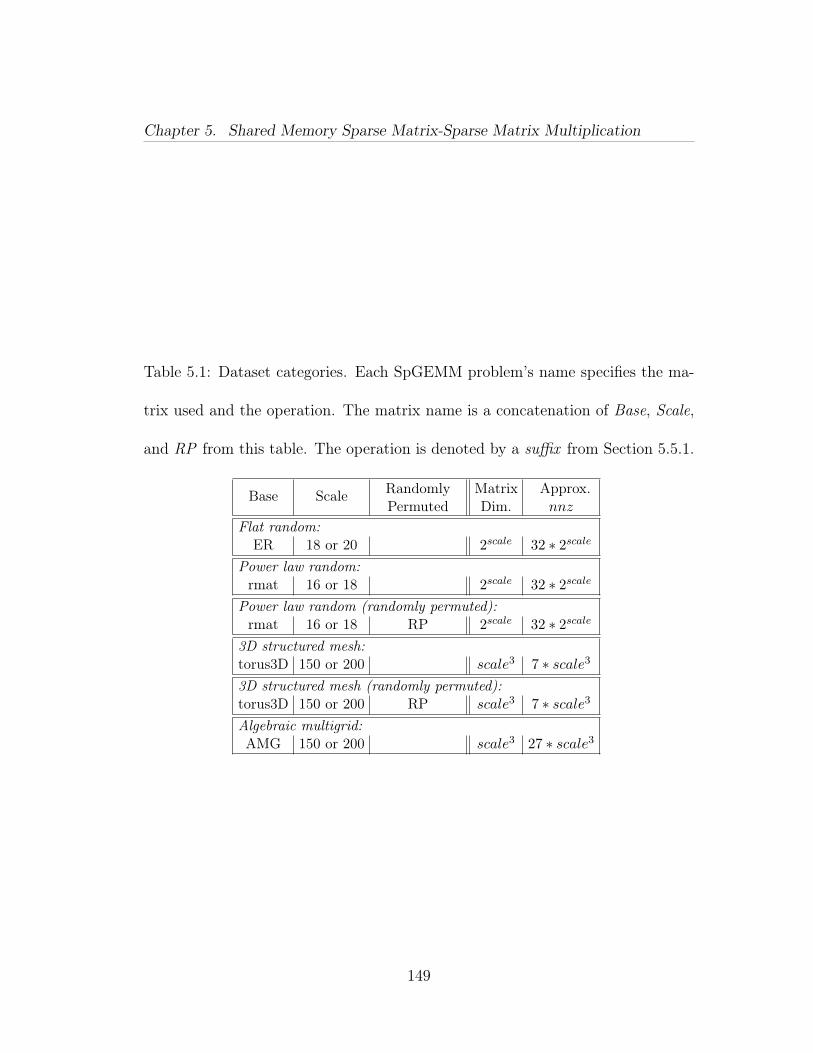
Chapter 5. Shared Memory Sparse Matrix-Sparse Matrix Multiplication
Table 5.1: Dataset categories. Each SpGEMM problem’s name specifies the ma-
trix used and the operation. The matrix name is a concatenation of Base, Scale,
and RP from this table. The operation is denoted by a suffix from Section 5.5.1.
Base Scale RandomlyPermuted
MatrixDim.
Approx.nnz
Flat random:ER 18 or 20 2scale 32 ∗ 2scale
Power law random:rmat 16 or 18 2scale 32 ∗ 2scale
Power law random (randomly permuted):rmat 16 or 18 RP 2scale 32 ∗ 2scale
3D structured mesh:torus3D 150 or 200 scale3 7 ∗ scale3
3D structured mesh (randomly permuted):torus3D 150 or 200 RP scale3 7 ∗ scale3
Algebraic multigrid:AMG 150 or 200 scale3 27 ∗ scale3
149

Chapter 5. Shared Memory Sparse Matrix-Sparse Matrix Multiplication
Problems
We generate SpGEMM problems from the datasets in several ways, each
marked by a distinct suffix to the dataset name:
1. Suffix _sq: We square the matrix.
2. Suffix _perm: We randomly permute the matrix rows by left multiplying it
by a generated random permutation matrix.
3. Suffix _sub: We select half the rows and half the columns of the matrix by
a triple product. This operation is also called SpRef.
4. Suffix _cont: Finally, we generate a set of three matrices that approximate
the contraction step of algebraic multigrid. We contract a dimension d
matrix with d3 cells to a dimension d/2 matrix with d3/8 cells. This entails
a R× A× P triple product.
The complete set of problems is described in Tables A.1 and A.2 in Ap-
pendix A.
Measurements
For each problem we calculate the number of non-zero arithmetic operations
(floating-point multiplies and additions) that occur. We then run each code/num-
ber of cores combination and record the elapsed time.
150
Chapter 5. Shared Memory Sparse Matrix-Sparse Matrix Multiplication
This data allows us to make a variety of comparisons. We can determine serial
efficiency by looking at the p = 1 results. We can determine strong scaling by
comparing increasing processor counts on the same problem, or weak scaling by
comparing larger generated problems on the same number of processors. We can
also compare to the serial CSparse code to determine when parallelism becomes
profitable.
Additionally, we probe QuadMat by profiling its behavior on one core.
5.5.2 Results
We ran QuadMat with blocksize threshold=max(50k, largest_nnz/80), with
a naïve index caching implementation, no post-processing phase, and only dense
versions of auxiliary data structures. The raw elapsed times for each problem are
listed in Tables A.3 and A.4 in Appendix A.
We analyze QuadMat’s performance from several angles. First, we get a broad
overview of the performance of all codes by comparing them to each other. We
then explore the effect of nonzero distribution on the runtimes, and the effect of
threshold choice on scalability. Finally we profile QuadMat execution.
151
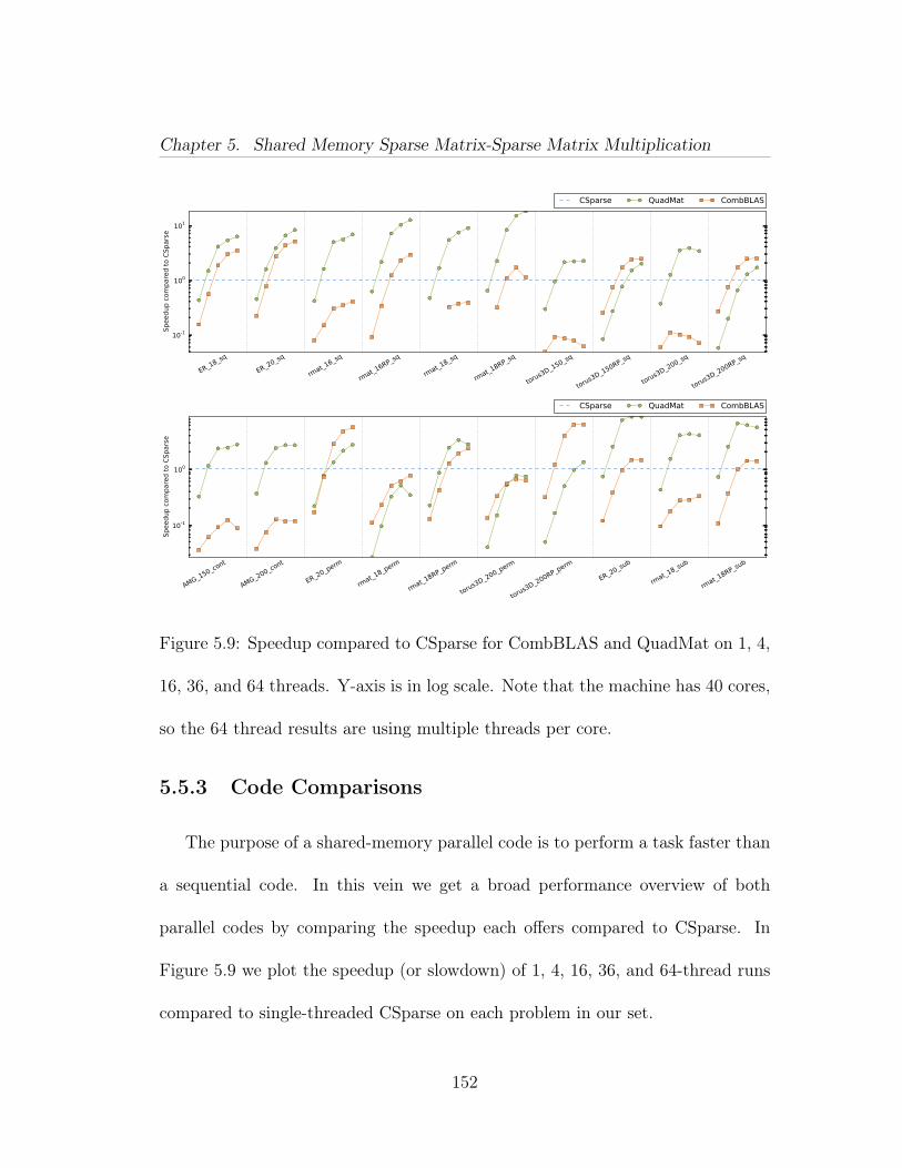
Chapter 5. Shared Memory Sparse Matrix-Sparse Matrix Multiplication
ER_18
_sq
ER_20
_sq
rmat_
16_sq
rmat_
16RP_s
q
rmat_
18_sq
rmat_
18RP_s
q
torus3
D_150_s
q
torus3
D_150R
P_sq
torus3
D_200_s
q
torus3
D_200R
P_sq
10-1
100
101
Speedup c
om
pare
d to C
Spars
e
CSparse QuadMat CombBLAS
AMG_150_c
ont
AMG_200_c
ont
ER_20
_perm
rmat_
18_pe
rm
rmat_
18RP_p
erm
torus3
D_200_p
erm
torus3
D_200R
P_perm
ER_20
_sub
rmat_
18_su
b
rmat_
18RP_s
ub
10-1
100
Speedup c
om
pare
d to C
Spars
e
CSparse QuadMat CombBLAS
Figure 5.9: Speedup compared to CSparse for CombBLAS and QuadMat on 1, 4,
16, 36, and 64 threads. Y-axis is in log scale. Note that the machine has 40 cores,
so the 64 thread results are using multiple threads per core.
5.5.3 Code Comparisons
The purpose of a shared-memory parallel code is to perform a task faster than
a sequential code. In this vein we get a broad performance overview of both
parallel codes by comparing the speedup each offers compared to CSparse. In
Figure 5.9 we plot the speedup (or slowdown) of 1, 4, 16, 36, and 64-thread runs
compared to single-threaded CSparse on each problem in our set.
152
Chapter 5. Shared Memory Sparse Matrix-Sparse Matrix Multiplication
We see many strengths of QuadMat and some weaknesses. QuadMat’s strongest
performance is on ER and RMAT matrix squares, and the AMG contraction and
submatrix extraction triple products. In 13 out of 20 problems QuadMat matches
CSparse performance with four cores or fewer. QuadMat shows good speedup
on the remaining problems, and does not match the CSparse sequential time on
only two out of 20 problems. This shows that there are clearly some significant
bottlenecks remaining.
We plot the same data as absolute values, namely FLOPS (or nonzero arith-
metic operations per second) achieved. Figure A.1 plots the same 1, 4, 16, 36,
and 64-thread runs for CombBLAS and QuadMat, but they can now be directly
compared to the FLOPS achieved by single-threaded CSparse. We observe that
on some problems all codes suffer reduced FLOPS, while all are faster on others.
The gap is large, two orders of magnitude.
Effects of Nonzero Distribution
We compare the effect of nonzero distribution on the various codes. This is
most evident when the same problem is available in a highly structured and a
randomly permuted form, namely torus squares. CSparse and QuadMat both
perform better on the structured version, CombBLAS on the randomized version.
There are two primary reasons for this.
153
Chapter 5. Shared Memory Sparse Matrix-Sparse Matrix Multiplication
Both CSparse and QuadMat use a dense lookup table for the columns (CSC
and CSC-like dense organizer, respectively). This makes sequential reads of the
columns very efficient. This locality is lost when the matrix is randomly permuted,
and FLOPS performance approaches that of the ER squares.
The hypersparse algorithm used by CombBLAS does not allow it to benefit
from this locality as much, so it is less affected by its loss. On the other hand,
CombBLAS uses a uniform block decomposition so the narrow-banded torus gives
a very unbalanced computational load. The random permutation provides a nearly
uniform nonzero distribution which allows CombBLAS to scale very well. Indeed
we see this effect in all problems; CombBLAS performs well on problems that
offer good load balancing and less well on ones that do not.
While load balance has a much weaker effect on QuadMat, we observe that
QuadMat struggles when the left factor is much more sparse and random than
the right factor, such as the permutation problems.
To help explain why sparse left factors are a performance bottleneck, we mea-
sure the observed utility of A organizer lookups. As described in Section 5.4, our
inner product computation performs lookups into A’s column organizer. The cost
of each miss (empty column) is amortized by the number of nonzero elements
discovered by hits. Each hit discovers at least one element.
154
Chapter 5. Shared Memory Sparse Matrix-Sparse Matrix Multiplication
We instrumented QuadMat to measure the total number of organizer lookups,
the number of hits, and the number of nonzeros discovered through each hit.
Dividing the latter by the total number of lookups gives us the lookup utility. Note
that these measured numbers are specific to each particular block decomposition
and will change with a different division threshold. See Table A.5 in Appendix A.
We quickly observe a pattern. QuadMat has good computational performance
on problems with high lookup utility and poor performance on problems with low
lookup utility. Indeed the worst performing permutation problems have terrible
lookup utility because nearly all lookups miss (due to the sparseness of the per-
mutation matrix) and the hits discover the minimum one element. This is the
hypersparse block effect.
CombBLAS is not affected by poor lookup utility because its hypersparse
sequential kernel does not perform lookups. In ongoing work we try to get the
best of both worlds. We mitigate the cost of the misses by switching to a DCSC-
like organizer on hypersparse blocks. Our design also permits us to selectively
perform the hypersparse algorithm on some block pairs then combine that result
with results using our Gustavson-derived kernel.
155
Chapter 5. Shared Memory Sparse Matrix-Sparse Matrix Multiplication
Strong Scaling
We are interested in what our code does on the same problem when it is given
more resources. In Figure 5.10 we plot the speedup of QuadMat on two to 36
cores. On a single socket laptop with 4 cores and 8 threads we see excellent
scaling even with two threads per core, but on our larger machine we see much
less benefit from multiple threads per core.
We observe excellent scaling with 2 and 4 threads on all problems, and good
scaling with 9 threads on most problems. Thread counts above 9 bring mixed
performance; most problems continue scaling; some stay about the same. We
hypothesize two reasons: insufficient parallelism and memory effects.
Our profile statistics in Table A.5 include the total compute task work (total
number of seconds) and the span (longest individual task). The ratio of those
two times is our potential parallelism. We see that for our chosen division thresh-
old, some problems (particularly AMG contraction) are indeed constrained by
insufficient potential parallelism.
To explore memory effects, we performed a set of runs in which we artificially
inflated the cost of arithmetic operations by looping them 5,000 times. This dras-
tically reduces the effects of memory latency, bandwidth, and caches. Figure 5.11
shows the results for three problems, comparing the speedup of the normal code
with the one with inflated arithmetic.
156
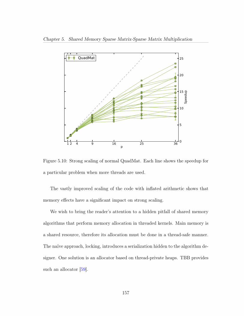
Chapter 5. Shared Memory Sparse Matrix-Sparse Matrix Multiplication
1 2 4 9 16 25 36p
0
5
10
15
20
25
Speedup
QuadMat
Figure 5.10: Strong scaling of normal QuadMat. Each line shows the speedup for
a particular problem when more threads are used.
The vastly improved scaling of the code with inflated arithmetic shows that
memory effects have a significant impact on strong scaling.
We wish to bring the reader’s attention to a hidden pitfall of shared memory
algorithms that perform memory allocation in threaded kernels. Main memory is
a shared resource, therefore its allocation must be done in a thread-safe manner.
The naïve approach, locking, introduces a serialization hidden to the algorithm de-
signer. One solution is an allocator based on thread-private heaps. TBB provides
such an allocator [59].
157
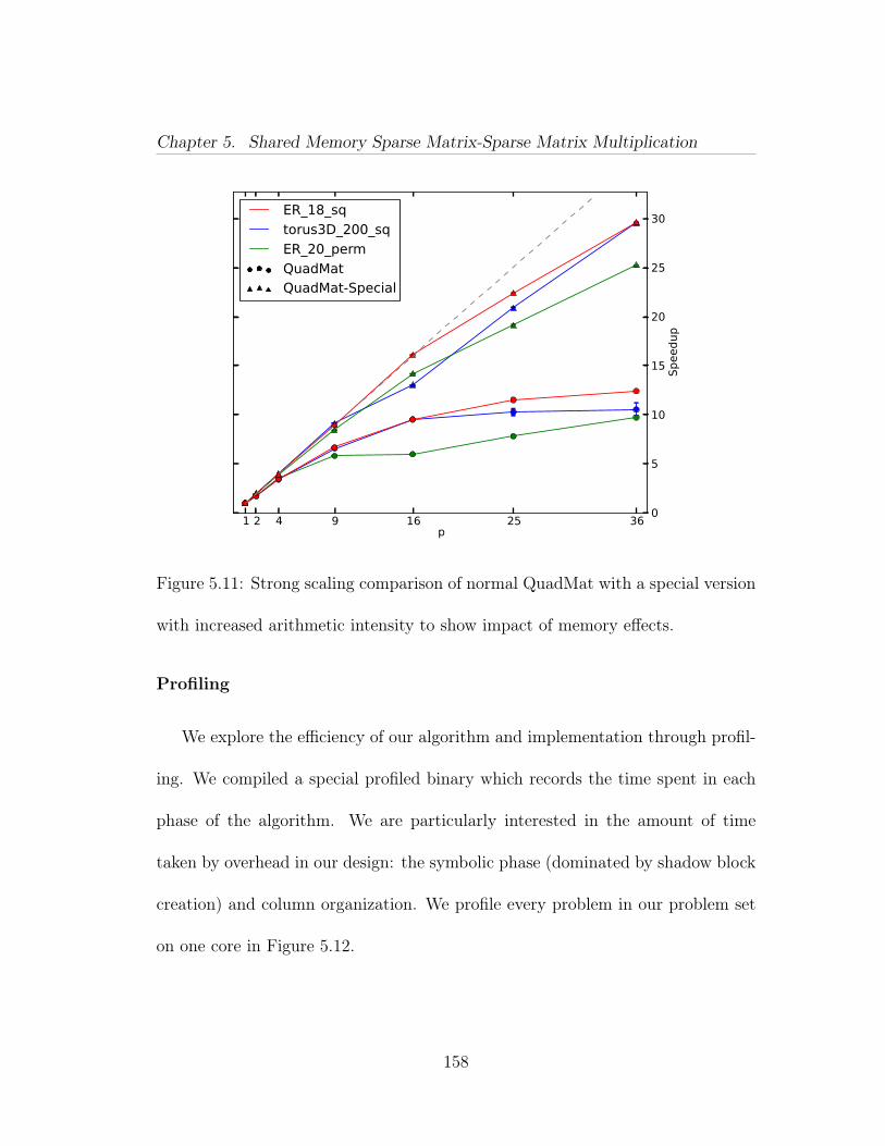
Chapter 5. Shared Memory Sparse Matrix-Sparse Matrix Multiplication
1 2 4 9 16 25 36p
0
5
10
15
20
25
30
Speedup
ER_18_sq
torus3D_200_sq
ER_20_perm
QuadMatQuadMat-Special
Figure 5.11: Strong scaling comparison of normal QuadMat with a special version
with increased arithmetic intensity to show impact of memory effects.
Profiling
We explore the efficiency of our algorithm and implementation through profil-
ing. We compiled a special profiled binary which records the time spent in each
phase of the algorithm. We are particularly interested in the amount of time
taken by overhead in our design: the symbolic phase (dominated by shadow block
creation) and column organization. We profile every problem in our problem set
on one core in Figure 5.12.
158
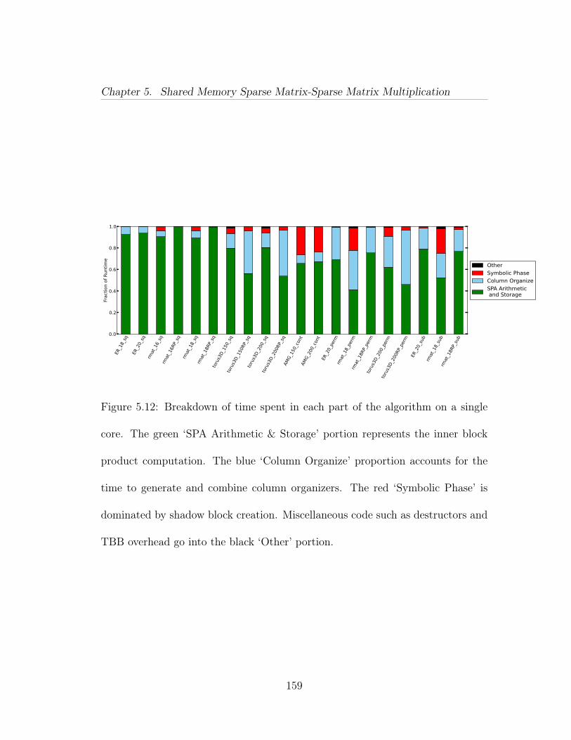
Chapter 5. Shared Memory Sparse Matrix-Sparse Matrix Multiplication
ER_18_sq
ER_20_sq
rmat_16_sq
rmat_16RP_sq
rmat_18_sq
rmat_18RP_sq
torus3D_150_sq
torus3D_150RP_sq
torus3D_200_sq
torus3D_200RP_sq
AMG_150_cont
AMG_200_cont
ER_20_perm
rmat_18_perm
rmat_18RP_perm
torus3D_200_perm
torus3D_200RP_perm
ER_20_sub
rmat_18_sub
rmat_18RP_sub
0.0
0.2
0.4
0.6
0.8
1.0
Fraction of Runtime
OtherSymbolic PhaseColumn OrganizeSPA Arithmetic and Storage
Figure 5.12: Breakdown of time spent in each part of the algorithm on a single
core. The green ‘SPA Arithmetic & Storage’ portion represents the inner block
product computation. The blue ‘Column Organize’ proportion accounts for the
time to generate and combine column organizers. The red ‘Symbolic Phase’ is
dominated by shadow block creation. Miscellaneous code such as destructors and
TBB overhead go into the black ‘Other’ portion.
159
Chapter 5. Shared Memory Sparse Matrix-Sparse Matrix Multiplication
The profile data shows that the symbolic phase, dominated by shadow block
creation, is not a significant portion of the runtime. The time spent in the symbolic
phase is less than 5% of runtime in all but four problems; the maximum is 25%.
Recall that this preliminary implementation includes only a naïve implementa-
tion of organizer caching. The need for efficient organization and organizer reuse
is suggested by the profile data; column organization accounts for between 15 and
45% of runtime for all but ER and RMAT square problems.
5.6 Discussion and Future Work
Our results show that, despite room for improvement, our algorithm has ex-
cellent performance and scaling. It offers significant speedup on some problems,
and we have strong leads on how to improve the cases where it does not.
Interestingly, the problems that QuadMat excels on are also the ones that are
sometimes considered the most difficult in the graph community: ones with a
small number of high-degree vertices.
Our continuing work includes two main improvements that should significantly
reduce or eliminate QuadMat’s weaknesses: organizer caching and a hierarchical
A-side organizer. These improvements should provide more latitude in automati-
cally choosing a good division threshold.
160
Chapter 5. Shared Memory Sparse Matrix-Sparse Matrix Multiplication
Our algorithm has potential to be extended in several ways.
We envision a triple product primitive that does not materialize the entire
intermediate product at any one time. This can be accomplished by merging the
two SpGEMMs’ symbolic phases. When done carefully with added destructor
tasks, the portions of the intermediate product needed for a portion of the second
SpGEMM can be materialized, used, and destroyed.
We also believe that the quadtree intermediate structure and triples leaf stor-
age enables computing AT ×B with similar complexity to A×B.
Additionally, we plan to take advantage of the block decomposition to use
serialization coupled with compression algorithms for savings in both memory
and memory bandwidth.
We may be able to save extra post-processing work by merging the subdivide
or coalesce step with the compute phase. This is a great application for auto-
tuning, as the appropriate choice needs to be made at runtime and according to
the actual workload.
We also emphasize that our leaf blocks provide a triples interface, but do not
mandate triples storage as an implementation. This enables features such as dense
blocks or generator blocks that emit triples but do not store them.
161
Chapter 5. Shared Memory Sparse Matrix-Sparse Matrix Multiplication
5.7 Conclusion
In conclusion, we summarize the key contributions of the design of our quadtree
sparse matrix multiplication algorithm:
• A method for elimination of explicit SpAdd operations that offers a signifi-
cant reduction in work for block-based SpGEMM.
• A split between symbolic and computational phases with temporary on-the-
fly data reorganization for simpler operations.
• An algorithm description that divides work into small tasks that can be
scheduled on any number of threads by third-party frameworks.
• A quadtree of triples blocks datastructure that has significant flexibility with
manageable overhead.
• A preliminary implementation that demonstrates these benefits.
162
Chapter 6
Complex Graph Algorithms in aDatabase Query Language
This chapter is based on a (second-place winning) entry to the YarcData Graph
Analytics Challenge [6]. An abridged version is published in SIAM Workshop
on Network Science [32]. A paper published in EBT/ICT Workshops [102] also
contains portions of this work.
6.1 Introduction
SPARQL is a powerful query language similar to SQL that operates on graphs
specified in the RDF format. RDF graphs are composed of triples, where each
triple consists of a subject, predicate, and object and specifies a directed edge
from subject to object with attribute predicate.
163
Chapter 6. Complex Graph Algorithms in a Database Query Language
SPARQL provides a rich way to query local neighborhoods. Our motivation
is to find a way to combine this with a global graph metric: clustering.
The driving application is clustering large clinical datasets, to help identify
potential disease causes. Autism researchers need to understand the underlying
causes of autism spectrum disorders, based on data from genetic (e.g., SNPs in
the GABA and glutamate pathways), medical history (diagnoses, prescriptions,
provider visits, including pre-natal/infant, esp. infant brain MRIs), environmental
(e.g., carcinogens, household chemicals), family medical history (i.e., parental psy-
chiatric history), and early-childhood intervention-strategy domains. In practice,
the patient base consists of thousands of individuals, with roughly 1M relation-
ships per patient [?].
6.2 Our Selected Clustering Algorithm
Peer Pressure [57, pp. 59-68] [97] is a clustering algorithm based on the ob-
servation that for a given graph clustering the cluster assignment of a vertex will
be the same as that of most of its neighbors.
The algorithm starts with an initial cluster assignment, such as each vertex
being in its own cluster. Each iteration performs an election at each vertex to
select which cluster that vertex should belong to at the end of the iteration. The
164
Chapter 6. Complex Graph Algorithms in a Database Query Language
votes are the cluster assignments of its neighbors. Ties are settled by selecting
the lowest cluster ID to maintain determinism, but could be settled arbitrarily.
The algorithm converges when two consecutive iterations have a (tunably) small
difference between them. Typically this leads to five to ten iterations on well-
clustered graphs.
This algorithm is also known by the name Label Propagation [92] in the physics
literature. Boldi et. al. [16] extend that work with Layered Label Propagation,
which accepts a parameter γ that selects between large relatively sparse clusters
and small relatively dense clusters.
6.3 Clustering Application
The design of the queries we use to implement Peer Pressure in SPARQL is
informed by the layout of the data we wish to cluster. We therefore first describe
our dataset, then the algorithm implementation.
6.3.1 Datasets
Clinical autism datasets are in general proprietary and protected by privacy
laws. Therefore, as a surrogate, we target our code for a dataset from the Mayo
165
Chapter 6. Complex Graph Algorithms in a Database Query Language
Clinic “Smackdown” project [101]. This dataset was synthesized by combining
data from various real-world sources to represent the nature of health-care records.
Despite being synthetic, this data was not freely available to outside researchers
such as ourselves for the majority of the project duration. We therefore chose to
benchmark our code using the cluster-realistic synthesis work of Pinar et al. [96].
We tailored our generator to produce data in a similar format to Smackdown.
Once we gained access to Smackdown data we were able to tailor our code to
work with it.
Smackdown data
The Smackdown data is a collection of database tables taken from public
sources (such as data.gov) which are then linked together to form a structure that
is subjectively similar to the clinical Autism data. The tables chosen have no par-
ticular meaning; they range from timezone information to air traffic networks and
botanical datasets. Their semantics are not important, in fact they are artificially
augmented with foreign keys that link tables together in an arbitrary way. While
a US Post Office location may have nothing to do with a flower, in aggregate these
links make the whole structure resemble the clinical Autism data such that it is
useful for testing.
The overall organization of the tables is as follows.
166
Chapter 6. Complex Graph Algorithms in a Database Query Language
• The data itself is all public, and comes from data.gov.
• There are on the order of 200-300 different SQL tables.
• Tables have between 15 and 60 columns.
• Tables have row counts anywhere from hundreds of thousands to tens of
millions.
• Each table has between 1 and 15 foreign keys.
The primary dataset is called dogdb-2G, as its size is about 2GB when stored
in a SQL database. The team at Mayo found this too small compared to their real
dataset, so they decided to augment the data with random rows generated using
a scheme that maintains the value distribution of the original dataset. Using this
method they have generated 20GB, 50GB, 80GB and 100GB datasets.
These SQL tables are converted to RDF to work on uRiKA. The 2G dataset
has 39M triples. The 100GB dataset has 5.6B triples with an uncompressed RDF
filesize size of 850GB.
The RDF is structured as follows:
• Each table is identified by a URI, with links to a Class.
• Each table column (identified by URI) contains two triples that declare the
column and link it to its table:
167
Chapter 6. Complex Graph Algorithms in a Database Query Language
– ?colURI <rdf:type> <rdf:Property> .
– ?colURI <rdf:label> "Table label" .
• Each table row has a URI (primary key).
• Each value in the table consists of a triple with a literal value: ?rowID
?colURI value .
• The foreign keys link two rows from different tables: ?rowID_tbl1 <xxx_Key_n>
?rowID_tbl2
• The column URI contains the string “Col” and foreign key URI “Key”.
Our goal is to cluster rows within a table but to also follow the foreign keys to
find clusters that span multiple tables. These clusters would show links between
multiple tables, helping the scientist link multiple potential factors for Autism.
6.3.2 Peer Pressure in SPARQL
The SPARQL implementation of Peer Pressure is relatively straight forward.
The algorithm maintains the clustering assignment of each vertex as its only state.
We store this state by creating RDF triples to represent an “inCluster” relation-
ship. We reuse names of existing vertices in the graph as cluster IDs, as the
IDs themselves are arbitrary and only have to be unique. A graph vertex would
168
Chapter 6. Complex Graph Algorithms in a Database Query Language
then be said to be in a particular cluster if there is an RDF triple specifying an
“inCluster” edge between the vertex and the cluster ID.
The cluster election at a vertex is equivalent to counting the number of length-
two paths between that vertex, one of its neighbors, and that neighbor’s cluster
ID (via an “inCluster” edge). The winner of the election is found by grouping
these paths by cluster ID, counting them, and selecting the cluster ID with the
maximum count.
Once the election is complete, we construct new edges between vertices and
their new clusters.
Since Peer Pressure is an iterative algorithm, the election and assignment need
to be performed multiple times to reach convergence. Our approach is to construct
actual RDF triples for each cluster assignment, then store them in a named graph
for retrieval by the election query of the next iteration. Once convergence is
reached the clustering can be read from the final named graph.
The query in Figure 6.1 is what one iteration’s election query looks like in
SPARQL. The query uses nested subqueries which tally the votes using a GROUP
BY and COUNT, and find the winner using a MAX.
This particular query only clusters edges with a “hasLink” relationship. This
relationship marks edges that passed the similarity metric, as embodied in the
initialization query mentioned earlier. The “hasLink” edges are stored in a separate
169
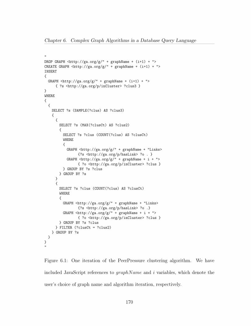
Chapter 6. Complex Graph Algorithms in a Database Query Language
"DROP GRAPH <http://ga.org/g/" + graphName + (i+1) + ">CREATE GRAPH <http://ga.org/g/" + graphName + (i+1) + ">INSERT{GRAPH <http://ga.org/g/" + graphName + (i+1) + ">
{ ?s <http://ga.org/p/inCluster> ?clus3 }}WHERE{{SELECT ?s (SAMPLE(?clus) AS ?clus3){{SELECT ?s (MAX(?clusCt) AS ?clus2){SELECT ?s ?clus (COUNT(?clus) AS ?clusCt)WHERE{GRAPH <http://ga.org/g/" + graphName + "Links>
{?s <http://ga.org/p/hasLink> ?o . }GRAPH <http://ga.org/g/" + graphName + i + ">
{ ?o <http://ga.org/p/inCluster> ?clus }} GROUP BY ?s ?clus
} GROUP BY ?s}{SELECT ?s ?clus (COUNT(?clus) AS ?clusCt)WHERE{GRAPH <http://ga.org/g/" + graphName + "Links>
{?s <http://ga.org/p/hasLink> ?o .}GRAPH <http://ga.org/g/" + graphName + i + ">
{ ?o <http://ga.org/p/inCluster> ?clus }} GROUP BY ?s ?clus
} FILTER (?clusCt = ?clus2)} GROUP BY ?s
}}"
Figure 6.1: One iteration of the PeerPressure clustering algorithm. We have
included JavaScript references to graphName and i variables, which denote the
user’s choice of graph name and algorithm iteration, respectively.
170
Chapter 6. Complex Graph Algorithms in a Database Query Language
named graph, and the result of each iteration of the algorithm is stored in its own
named graph as well. Each stored iteration consists of only the “inCluster” edges,
and there is only one such edge per vertex. Therefore, depending on average
degree, each stored iteration is small compared to the total number of triples in
the original graph. We compare results of consecutive iterations with each other
to determine convergence.
Note that our driver code is written in JavaScript to run queries remotely (see
Section 6.4). We kept references to our JavaScript variables, graphName and i,
which denote the name of the graph and the iteration count, respectively.
6.3.3 Discussion
We believe that Peer Pressure is a good fit for a SPARQL-based implementa-
tion because its inherently local nature fits well with the SPARQL paradigm. The
heart of the algorithm, the election, has natural analogues in SPARQL aggregate
functions. We also observe that our queries are highly dependent on large joins,
which give uRiKA an advantage over its competition (See Section 6.5).
We note that our approach to the Peer Pressure algorithm, i.e. keeping algo-
rithm state and iterating, makes possible a wide variety of other graph algorithms
to be performed using SPARQL queries. For example, breadth-first search could
be implemented using a similar approach, with state maintained by adding links
171
Chapter 6. Complex Graph Algorithms in a Database Query Language
to “nFrontier” and “discovered” edges as the queries traverse the graph. More
complex state schemes could enable algorithms such as PageRank and Between-
ness Centrality.
6.4 Workflow and Implementation
We have divided our workflow into three distinct steps: Conversion, Cluster
Algorithm, Results. Each is described below. SPARQL backends typically have
an interface similar to SQL: individual queries are sent to the engine and results
returned. This can occur at a manual administration console, or it can be scripted
using a database connection interface. We chose to implement our workflow in
an HTML+JavaScript webpage which guides the user through the steps and can
automate query execution.
6.4.1 Implementation in HTML/JavaScript
Our Peer Pressure implementation consists of several queries per iteration. We
chose to combine all these queries into a JavaScript function whose only logic is
a loop.
172
Chapter 6. Complex Graph Algorithms in a Database Query Language
The script is pointed at a SPARQL endpoint such as uRiKA or Apache Fuseki.
A single click of a button automatically runs all the Peer Pressure queries in the
right order and stops upon convergence.
We found it useful to automate some of the other steps of the workflow as
well. A large portion of the data preparation is also be done via this webpage.
The results can be fetched through several pre-made aggregation queries.
Apart from user friendliness, a benefit of using HTML/JavaScript is that it
allows easy formatting and visualization. A screenshot of our (admittedly crude
and developer-oriented) interface is in Figure 6.5.
6.4.2 Conversion Stage
Our Peer Pressure clustering implementation does not work on the data di-
rectly, instead it follows explicit “hasLink” relationships as denoted by a triple
with a “hasLink” predicate. As such, we need a step which converts the raw data
into these relationships.
The conversion means that edges are created between table rows that are
similar “enough”. In fact, this means that this step is one of the main ways that
the scientist influences the computation. The scientist must find specify what
they deem to be a good similarity metric for a particular table or even a particular
173
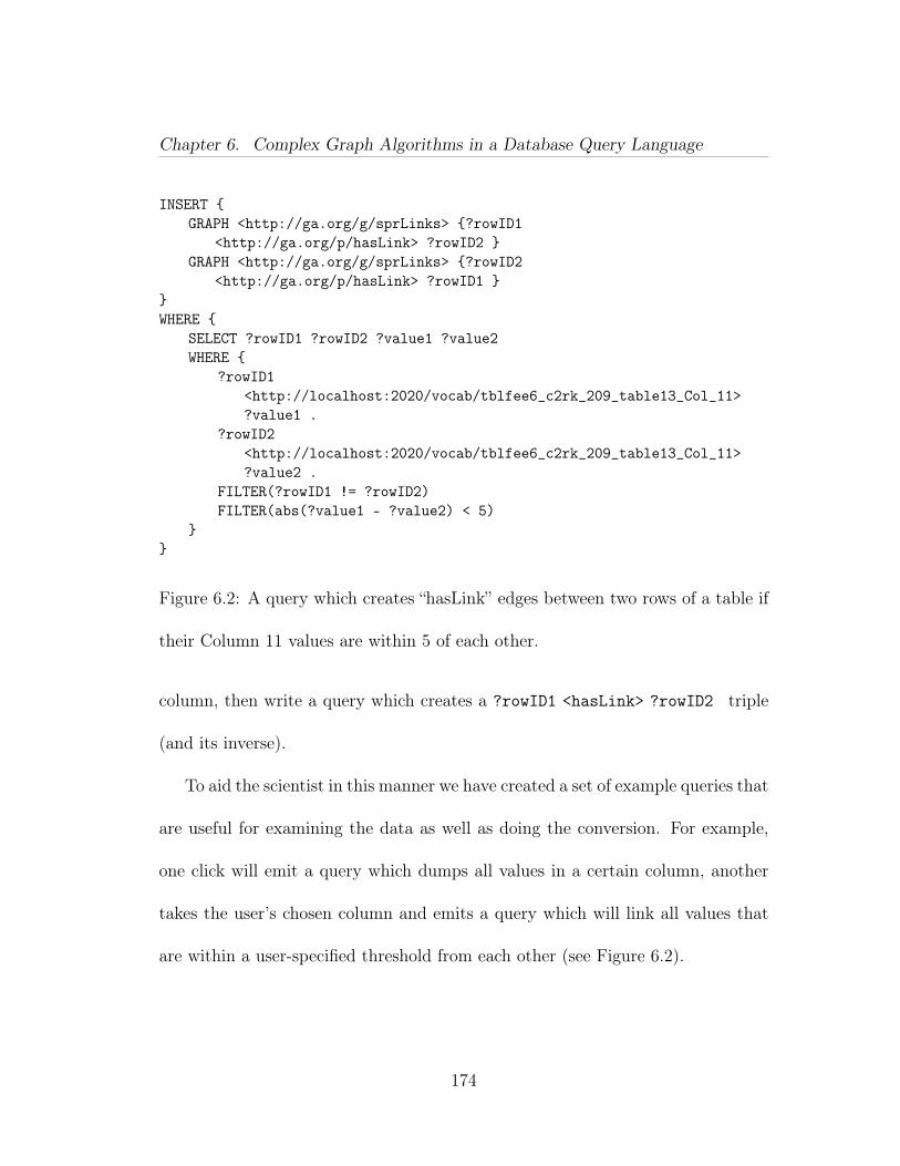
Chapter 6. Complex Graph Algorithms in a Database Query Language
INSERT {GRAPH <http://ga.org/g/sprLinks> {?rowID1
<http://ga.org/p/hasLink> ?rowID2 }GRAPH <http://ga.org/g/sprLinks> {?rowID2
<http://ga.org/p/hasLink> ?rowID1 }}WHERE {
SELECT ?rowID1 ?rowID2 ?value1 ?value2WHERE {
?rowID1<http://localhost:2020/vocab/tblfee6_c2rk_209_table13_Col_11>?value1 .
?rowID2<http://localhost:2020/vocab/tblfee6_c2rk_209_table13_Col_11>?value2 .
FILTER(?rowID1 != ?rowID2)FILTER(abs(?value1 - ?value2) < 5)
}}
Figure 6.2: A query which creates “hasLink” edges between two rows of a table if
their Column 11 values are within 5 of each other.
column, then write a query which creates a ?rowID1 <hasLink> ?rowID2 triple
(and its inverse).
To aid the scientist in this manner we have created a set of example queries that
are useful for examining the data as well as doing the conversion. For example,
one click will emit a query which dumps all values in a certain column, another
takes the user’s chosen column and emits a query which will link all values that
are within a user-specified threshold from each other (see Figure 6.2).
174
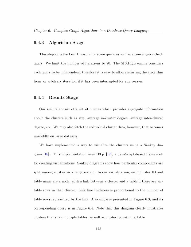
Chapter 6. Complex Graph Algorithms in a Database Query Language
6.4.3 Algorithm Stage
This step runs the Peer Pressure iteration query as well as a convergence check
query. We limit the number of iterations to 20. The SPARQL engine considers
each query to be independent, therefore it is easy to allow restarting the algorithm
from an arbitrary iteration if it has been interrupted for any reason.
6.4.4 Results Stage
Our results consist of a set of queries which provides aggregate information
about the clusters such as size, average in-cluster degree, average inter-cluster
degree, etc. We may also fetch the individual cluster data; however, that becomes
unwieldly on large datasets.
We have implemented a way to visualize the clusters using a Sankey dia-
gram [18]. This implementation uses D3.js [17], a JavaScript-based framework
for creating visualizations. Sankey diagrams show how particular components are
split among entities in a large system. In our visualization, each cluster ID and
table name are a node, with a link between a cluster and a table if there are any
table rows in that cluster. Link line thickness is proportional to the number of
table rows represented by the link. A example is presented in Figure 6.3, and its
corresponding query is in Figure 6.4. Note that this diagram clearly illustrates
clusters that span multiple tables, as well as clustering within a table.
175
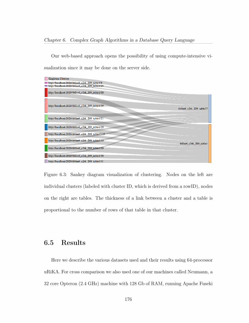
Chapter 6. Complex Graph Algorithms in a Database Query Language
Our web-based approach opens the possibility of using compute-intensive vi-
sualization since it may be done on the server side.
Figure 6.3: Sankey diagram visualization of clustering. Nodes on the left are
individual clusters (labeled with cluster ID, which is derived from a rowID), nodes
on the right are tables. The thickness of a link between a cluster and a table is
proportional to the number of rows of that table in that cluster.
6.5 Results
Here we describe the various datasets used and their results using 64-processor
uRiKA. For cross comparison we also used one of our machines called Neumann, a
32 core Opteron (2.4 GHz) machine with 128 Gb of RAM, running Apache Fuseki
176
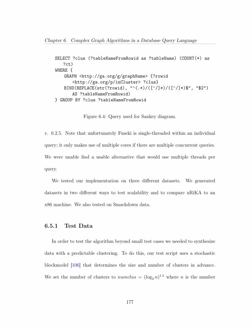
Chapter 6. Complex Graph Algorithms in a Database Query Language
SELECT ?clus (?tableNameFromRowid as ?tableName) (COUNT(*) as?ct)
WHERE {GRAPH <http://ga.org/g/graphName> {?rowid
<http://ga.org/p/inCluster> ?clus}BIND(REPLACE(str(?rowid), "^(.*)/([^/]*)/([^/]*)$", "$2")
AS ?tableNameFromRowid)} GROUP BY ?clus ?tableNameFromRowid
Figure 6.4: Query used for Sankey diagram.
v. 0.2.5. Note that unfortunately Fuseki is single-threaded within an individual
query; it only makes use of multiple cores if there are multiple concurrent queries.
We were unable find a usable alternative that would use multiple threads per
query.
We tested our implementation on three different datasets. We generated
datasets in two different ways to test scalability and to compare uRiKA to an
x86 machine. We also tested on Smackdown data.
6.5.1 Test Data
In order to test the algorithm beyond small test cases we needed to synthesize
data with a predictable clustering. To do this, our test script uses a stochastic
blockmodel [106] that determines the size and number of clusters in advance.
We set the number of clusters to numclus = (log2 n)1.5 where n is the number
177
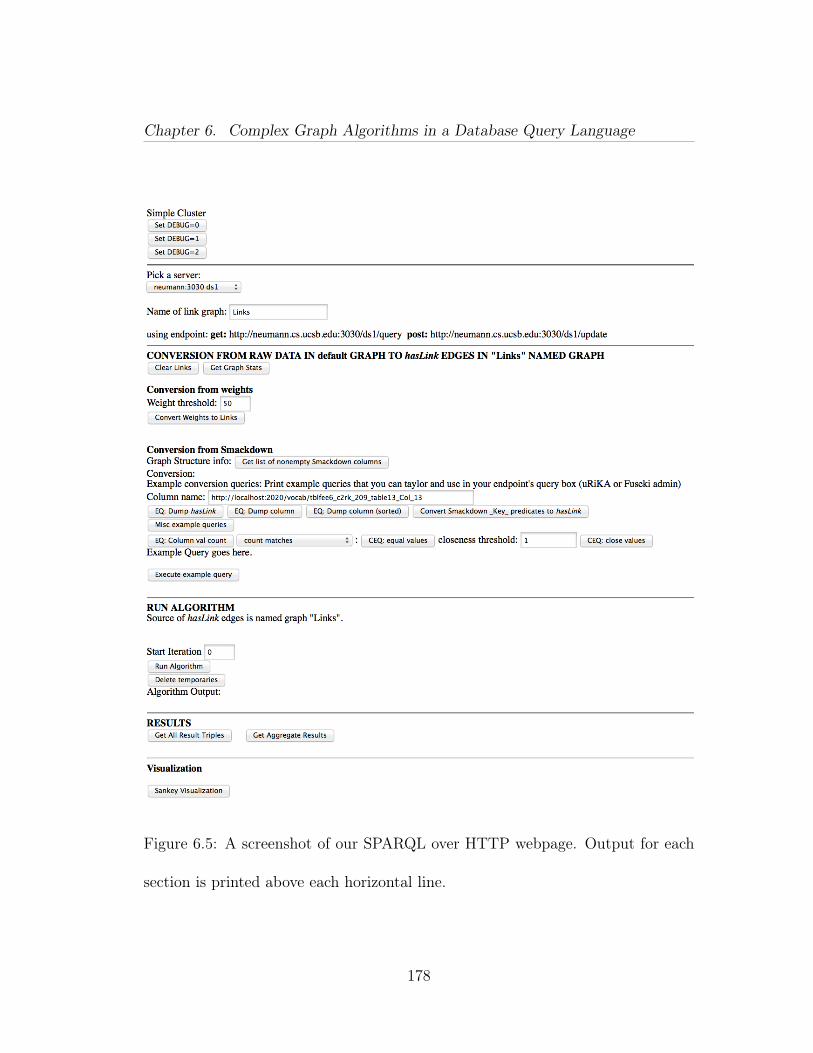
Chapter 6. Complex Graph Algorithms in a Database Query Language
Figure 6.5: A screenshot of our SPARQL over HTTP webpage. Output for each
section is printed above each horizontal line.
178
Chapter 6. Complex Graph Algorithms in a Database Query Language
of vertices. The generator then considers all edge pairs and adds intercluster
edges with probability 0.02 and intracluster edges with probability 0.1. Thus the
clustering algorithm should find the desired clusters with high probability. The
data we generated contained 100,000 vertices and 15,736,484 triples. The triples
were assigned a random similarity measure as described above to test the threshold
conversion query. On uRiKA the clustering converged in 5 iterations after 200.2
seconds. On Neumann the first update alone took about 9 hours with the first
iteration completing in just under 12 hours. The whole algorithm did not finish.
6.5.2 BTER Data
The BTER data was generated using the Matlab generator written by Pinar
et al. [96]. We then wrote a script to convert the result of this generator into RDF
triples. The parameters we used in the generator along with specifying a power-
law degree distribution are γ = 2, maxdegree = 100, ρinit = 0.99, ρdecay = 0.8.
The BTER dataset we used contained 1,643,915 vertices and 7,332,102 triples.
On uRiKA this graph did not converge as the maximum number of iterations is
20, but it did complete these iterations in 3 hours, 9 minutes.
179
Chapter 6. Complex Graph Algorithms in a Database Query Language
6.5.3 Smackdown Data
Working with the full Smackdown data posed a challenge. The amount of data
is vast, and we only had access to it for a relatively short time. We loaded a small
(100,000 triple) subset of the 2G dataset on our Fuseki machine and were able to
debug our script with it. We discovered that this made debugging our queries and
driver script much easier, as uRiKA does not provide a way to kill a query that’s
unexpectedly too slow (at least to end users).
We experimented with the 20G dataset (1.3B triples) on uRiKA. We discovered
several difficulties that are not clear on smaller datasets.
First, every query takes a very long time, no matter how simple it is. We
discovered that this is largely due to the fact that even though our queries narrow
down their operands to a relatively small subset of the entire graph, the entire
graph is still traversed. We came up with several potential solutions, such as
using named graphs to shard the data into chunks. For example, each table or
even column can have its own named graph. This would mean that the conversion
queries would operate on a very small subset of the graph.
Second, the need for “hasLink” edges between similar rows results in a potential
quadratic expansion. While this was obvious from the start, this property began
to pose significant problems on the large dataset. Specifically, even if the result
has been narrowed down, the computation is still very expensive. We are exploring
180
Chapter 6. Complex Graph Algorithms in a Database Query Language
ways to alleviate this problem, such as using explicit groups and intermediate links
to reduce the amount of “hasLink” edges. This requires changing the PeerPressure
queries to support groups, which is ongoing work.
6.6 Conclusion
We have managed to create an entire workflow solution for clustering RDF
graphs using SPARQL. This is an important result because it shows that a global
graph metric like clustering can be implemented in SPARQL. We also propose
that our method is easily extendible to other graph algorithms not previously
available to SPARQL users.
We’ve also shown that uRiKA really shines on a variety of queries as compared
to x86 servers. This has allowed us to cluster very large RDF graphs, something
not possible on lesser hardware.
We’ve also shown that an HTML/JavaScript driver has multiple advantages.
It allows automation of boilerplate tasks, makes data exploration simpler, and
allows for easy visualization. It makes a scientist’s life easier.
181
Chapter 7
Conclusions
This thesis advances the state of the art in computation on very large graphs
by enabling efficient implementations of interfaces to algebraic primitives.
We have put non-HPC expert graph analysts at the forefront. We bring them
flexible primitives and algorithms exposed in a high productivity language, with-
out compromising on performance or scalability.
We also contribute a new sparse matrix datastructure and sparse matrix mul-
tiplication algorithm to better take advantage of large shared memory machines
or nodes in hybrid clusters.
182
Bibliography
[1] Active Record - Object-Relation Mapping Put on Rails. http://ar.rubyonrails.org, 2012.
[2] Apache Gigraph. http://giraph.apache.org, 2013.
[3] Apache Hama. http://hama.apache.org, 2013.
[4] Performance Application Programming Interface (PAPI). http://icl.cs.utk.edu/papi/, 2013.
[5] PyPy. http://pypy.org, 2013.
[6] YarcData Graph Analytics Challenge, April 2013.
[7] C. Avery. Giraph: large-scale graph processing infrastructure on hadoop.Proceedings of Hadoop Summit. Santa Clara, USA, 2011.
[8] D. Bader, J. Berry, A. Amos-Binks, D. Chavarría-Miranda, C. Hastings,K. Madduri, and S. Poulos. STINGER: Spatio-Temporal Interaction Net-works and Graphs (STING) extensible representation. Georgia Institute ofTechnology, Tech. Rep, 2009.
[9] D. Bader, J. Gilbert, J. Kepner, D. Koester, E. Loh, K. Madduri, B. Mann,and T. Meuse. HPCS Scalable Synthetic Compact Applications #2.http://graphanalysis.org/benchmark.
[10] D. Bader, S. Kintali, K. Madduri, and M. Mihail. Approximating Between-ness Centrality. In A. Bonato and F. Chung, editors, Algorithms and Mod-els for the Web-Graph, volume 4863 of Lecture Notes in Computer Science,pages 124–137. Springer Berlin/Heidelberg, 2007.
[11] D. A. Bader and K. Madduri. SNAP, small-world network analysis andpartitioning: An open-source parallel graph framework for the exploration of
183
Bibliography
large-scale networks. In Proc. IEEE Int. Symposium on Parallel&DistributedProcessing, pages 1–12, 2008.
[12] S. Beamer, K. Asanović, and D. Patterson. Direction-optimizing breadth-first search. Scientific Programming, 21(3):137–148, 2013.
[13] S. Beamer, A. Buluç, K. Asanovic, and D. Patterson. Distributed memorybreadth-first search revisited: Enabling bottom-up search. In Proceedings ofthe 2013 IEEE 27th International Symposium on Parallel and DistributedProcessing Workshops and PhD Forum, pages 1618–1627. IEEE ComputerSociety, 2013.
[14] J. Berry, B. Hendrickson, S. Kahan, and P. Konecny. Software and Algo-rithms for Graph Queries on Multithreaded Architectures. In Proc. Work-shop on Multithreaded Architectures and Applications. IEEE Press, 2007.
[15] D. Bickson. Gaussian Belief Propagation: Theory and Application. CoRR,abs/0811.2518, 2008.
[16] P. Boldi, M. Rosa, M. Santini, and S. Vigna. Layered label propagation: amultiresolution coordinate-free ordering for compressing social networks. InProceedings of the 20th international conference on World wide web - WWW’11, pages 587–596, New York, New York, USA, 2011. ACM Press.
[17] M. Bostock. Data-driven documents (d3.js), a visualization framework forinternet browsers running javascript, 2012.
[18] M. Bostock. Sankey diagrams, May 2012.http://bost.ocks.org/mike/sankey/.
[19] U. Brandes. A Faster Algorithm for Betweenness Centrality. J. Math.Sociol., 25(2):163–177, 2001.
[20] S. Brohée and J. van Helden. Evaluation of clustering algorithms for protein-protein interaction networks. BMC Bioinformatics, 7:488, 2006.
[21] A. Buluç, E. Duriakova, A. Fox, J. R. Gilbert, S. Kamil, A. Lugowski,L. Oliker, and S. Williams. High-productivity and high-performance anal-ysis of filtered semantic graphs. In 27th IEEE International Symposium onParallel and Distributed Processing (IPDPS 2013), May 2013.
[22] A. Buluç, J. T. Fineman, M. Frigo, J. R. Gilbert, and C. E. Leiserson. Par-allel sparse matrix-vector and matrix-transpose-vector multiplication using
184
Bibliography
compressed sparse blocks. In Proc. 21st Symp. on Parallelism in Algorithmsand Arch., 2009.
[23] A. Buluç, A. Fox, J. R. Gilbert, S. Kamil, A. Lugowski, L. Oliker, andS. Williams. High-performance analysis of filtered semantic graphs. InProceedings of the 21st international conference on Parallel architecturesand compilation techniques, PACT ’12, pages 463–464, New York, NY, USA,2012. ACM. extended abstract.
[24] A. Buluç and J. Gilbert. The Combinatorial BLAS: Design, implemen-tation, and applications. The International Journal of High PerformanceComputing Applications, 25(4):496–509, 2011.
[25] A. Buluç and J. R. Gilbert. On the Representation and Multiplication ofHypersparse Matrices. In Proc. IPDPS, April 2008.
[26] A. Buluç and K. Madduri. Parallel breadth-first search on distributed mem-ory systems. In Proc. Supercomputing, 2011.
[27] B. Catanzaro, S. Kamil, Y. Lee, K. Asanović, J. Demmel, K. Keutzer,J. Shalf, K. Yelick, and A. Fox. SEJITS: Getting Productivity and Per-formance With Selective Embedded JIT Specialization. In PMEA, 2009.
[28] T. Davis. Direct Methods for Sparse Linear Systems (Fundamentals of Al-gorithms 2). Society for Industrial and Applied Mathematics, Philadelphia,PA, 2006.
[29] T. Davis and Y. Hu. The University of Florida Sparse Matrix Collection.ACM Transactions on Mathematical Software, to appear, 2011.
[30] T. A. Davis. Direct Methods for Sparse Linear Systems. SIAM, Philadelphia,Sept 2006.
[31] J. Dean and S. Ghemawat. MapReduce: simplified data processing on largeclusters. In Proc. 6th Symposium on Operating System Design and Imple-mentation, pages 137–149, Berkeley, CA, USA, 2004. USENIX Association.
[32] K. Deweese, J. R. Gilbert, A. Lugowski, and S. Reinhardt. Graph clusteringin sparql. In SIAM Workshop on Network Science, 2013.
[33] B. Dezső, A. Jüttner, and P. Kovács. Lemon–an open source c++ graph tem-plate library. Electronic Notes in Theoretical Computer Science, 264(5):23–45, 2011.
185
Bibliography
[34] B. Dorow. A Graph Model for Words and their Meanings. PhD thesis,Universität Stuttgart, 2006.
[35] A. Enright, S. Van Dongen, and C. Ouzounis. An efficient algorithm forlarge-scale detection of protein families. Nucl. Acids Res., 30(7):1575–1584,2002.
[36] P. Erdős and A. Rényi. On the evolution of random graphs. In Publicationof the Mathematical Institute of the Hungarian Academy of Sciences, pages17–61, 1960.
[37] P. Erdős and A. Rényi. On random graphs. Publicationes Mathematicae,6(1):290–297, 1959.
[38] M. Fowler. Domain Specific Languages. Addison-Wesley Professional, 2010.
[39] L. Freeman. A Set of Measures of Centrality Based on Betweenness. So-ciometry, 40(1):35–41, 1977.
[40] J. D. Frens and D. S. Wise. Auto-blocking matrix-multiplication or trackingBLAS3 performance from source code. SIGPLAN Not., 32(7):206–216, June1997.
[41] J. D. Frens and D. S. Wise. QR factorization with Morton-ordered quadtreematrices for memory re-use and parallelism. In Proceedings of the NinthACM SIGPLAN Symposium on Principles and Practice of Parallel Pro-gramming, PPoPP ’03, pages 144–154, New York, NY, USA, 2003. ACM.
[42] J. Gilbert, C. Moler, and R. Schreiber. Sparse matrices in MATLAB: Designand implementation. SIAM J. Matrix Anal. Appl, 13:333–356, 1992.
[43] J. Gilbert, C. Moler, and R. Schreiber. Sparse matrices in MATLAB: Designand implementation. SIAM Journal on Matrix Analysis and Applications,13(1):333–356, 1992.
[44] J. R. Gilbert. Sparse matrices and graphs: There and back again. Talkgiven at SVG 70, Stanford, 1 2014.
[45] J. R. Gilbert. xxxxxxx. Talk given at Graph Algorithms Building BlocksWorkshop (GABB’14) in conjunction with IPDPS’14, 5 2014.
[46] J. S. Golan. Semirings and their Applications. Springer, 1999.
186
Bibliography
[47] A. Goldberg and R. Werneck. Computing Point-to-Point Shortest Pathsfrom External Memory. In Proc. 7th Workshop on Algorithm Engineeringand Experiments (ALENEX05), pages 26–40, 2005.
[48] J. E. Gonzalez, Y. Low, H. Gu, D. Bickson, and C. Guestrin. PowerGraph:Distributed graph-parallel computation on natural graphs. In Proceedingsof the 10th USENIX Symposium on Operating Systems Design and Imple-mentation (OSDI), pages 17–30, 2012.
[49] Graph500. http://www.graph500.org.
[50] D. Gregor and A. Lumsdaine. The Parallel BGL: A Generic Library forDistributed Graph Computations. In Proc. Workshop on Parallel/High-Performance Object-Oriented Scientific Computing (POOSC’05), 2005.
[51] F. G. Gustavson. Two fast algorithms for sparse matrices: Multiplicationand permuted transposition. ACM Trans. Math. Softw., 4(3):250–269, 1978.
[52] M. A. Heroux, R. A. Bartlett, V. E. Howle, R. J. Hoekstra, J. J. Hu, T. G.Kolda, R. B. Lehoucq, K. R. Long, R. P. Pawlowski, E. T. Phipps, A. G.Salinger, H. K. Thornquist, R. S. Tuminaro, J. M. Willenbring, A. Williams,and K. S. Stanley. An Overview of the Trilinos Project. ACM Trans. Math.Softw., 31:397–423, September 2005.
[53] S. Hong, H. Chafi, E. Sedlar, and K. Olukotun. Green-Marl: a DSL foreasy and efficient graph analysis. In Proceedings of the seventeenth inter-national conference on Architectural Support for Programming Languagesand Operating Systems, ASPLOS ’12, pages 349–362, New York, NY, 2012.ACM.
[54] S. Kamil, D. Coetzee, S. Beamer, H. Cook, E. Gonina, J. Harper, J. Morlan,and A. Fox. Portable parallel performance from sequential, productive,embedded domain specific languages. In PPoPP’12, 2012.
[55] U. Kang, C. Tsourakakis, and C. Faloutsos. PEGASUS: A Peta-Scale GraphMining System - Implementation and Observations. In Data Mining, 2009.ICDM’09. Ninth IEEE International Conference on, pages 229–238. IEEE,2009.
[56] G. Karypis, K. Schloegel, and V. Kumar. ParMETIS: Parallel Graph Par-titioning and Sparse Matrix Ordering Library. Technical report, Dept. ofComputer Science, University of Minnesota, 1997.
187
Bibliography
[57] J. Kepner and J. R. Gilbert, editors. Graph Algorithms in the Language ofLinear Algebra. Society for Industrial and Applied Mathematics, 2011.
[58] P. Konecny. Introducing the Cray XMT. Cray User Group meeting (CUG),2007.
[59] A. Kukanov and M. J. Voss. The foundations for scalable multi-core softwarein Intel Threading Building Blocks. Intel Technology Journal, 11(4):309 –322, 2007.
[60] H. Kwak, C. Lee, H. Park, and S. Moon. What is Twitter, a social networkor a news media? In WWW ’10: Proceedings of the 19th internationalconference on World wide web, pages 591–600, New York, NY, USA, 2010.ACM.
[61] O. Lassila and R. Swick. Resource Description Framework (RDF) Modeland Syntax Specification. W3c recommendation, W3C, Feb 1999.
[62] L. Lee, A. Lumsdaine, and J. Siek. The Boost GraphLibrary: User Guide and Reference Manual, 2002.www.osl.iu.edu/publications/Year/2002.complete.php.
[63] R. Lehoucq, D. Sorensen, and C. Yang. ARPACK Users’ Guide: Solution ofLarge Scale Eigenvalue Problems with Implicitly Restarted Arnoldi Methods.SIAM, 1998.
[64] X. Lei, X. Ostwald, J. Hu, C. Qiu, C. Porcaro, A. P. Bagshaw, and D. Yao.Multimodal functional network connectivity: an EEG-fMRI fusion in net-work space. PloS one, 6(9):e24642, 2011.
[65] D. Leijen and E. Meijer. Domain specific embedded compilers. In Proc.Conference on Domain-Specific Languages, DSL’99, pages 9–9, Berkeley,CA, 1999. USENIX.
[66] J. Leskovec, D. Chakrabarti, J. Kleinberg, and C. Faloutsos. Realistic,Mathematically Tractable Graph Generation and Evolution, Using Kro-necker Multiplication. In PKDD, pages 133–145. Springer, 2005.
[67] J. Leskovec, D. Chakrabarti, J. Kleinberg, and C. Faloutsos. Realistic,Mathematically Tractable Graph Generation and Evolution, Using Kro-necker Multiplication. In PKDD, pages 133–145, 2005.
[68] X. Li, J. Demmel, J. Gilbert, L. Grigori, and M. Shao. SuperLU Users’Guide, 2010.
188
Bibliography
[69] Y. Low, J. Gonzalez, A. Kyrola, D. Bickson, C. Guestrin, and J. Hellerstein.GraphLab: A New Parallel Framework for Machine Learning. In Conferenceon Uncertainty in Artificial Intelligence (UAI), Catalina Island, California,July 2010.
[70] M. Luby. A simple parallel algorithm for the maximal independent setproblem. In Proc. ACM symposium on Theory of computing, STOC ’85,pages 1–10, New York, NY, 1985. ACM.
[71] M. Luby. A simple parallel algorithm for the maximal independent setproblem. SIAM journal on computing, 15(4):1036–1053, 1986.
[72] A. Lugowski, D. Alber, A. Buluç, J. R. Gilbert, S. Reinhardt, Y. Teng,and A. Waranis. A flexible open-source toolbox for scalable complex graphanalysis. In Proceedings of the Twelfth SIAM International Conference onData Mining (SDM12), pages 930–941, April 2012.
[73] A. Lugowski, A. Buluç, J. Gilbert, and S. Reinhardt. Scalable complex graphanalysis with the knowledge discovery toolbox. In International Conferenceon Acoustics, Speech, and Signal Processing (ICASSP), 2012.
[74] A. Lugowski, A. Buluç, J. Gilbert, and S. Reinhardt. Scalable ComplexGraph Analysis with the Knowledge Discovery Toolbox. In Int. Conferenceon Acoustics, Speech, and Signal Processing, 2012.
[75] A. Lugowski and J. R. Gilbert. Efficient sparse matrix-matrix multiplicationon multicore architectures. Technical Report UCSB/CS-2014-04, ComputerScience Dept., University of California, Santa Barbara, May 2014.
[76] A. Lugowski and J. R. Gilbert. Efficient sparse matrix-matrix multiplicationon multicore architectures. In SIAM Workshop on Combinatorial ScientificComputing (CSC14), July 2014.
[77] A. Lugowski, S. Kamil, A. Buluç, S. Williams, E. Duriakova, L. Oliker,A. Fox, and J. R. Gilbert. Parallel processing of filtered queries in attributedsemantic graphs. Journal of Parallel and Distributed Computing (JPDC),Accepted.
[78] G. Malewicz, M. Austern, A. Bik, J. Dehnert, I. Horn, N. Leiser, and G. Cza-jkowski. Pregel: A System for Large-Scale Graph Processing. In Proceedingsof the 2010 International Conference on Management of Data, SIGMOD ’10,pages 135–146, New York, NY, USA, 2010. ACM.
189
Bibliography
[79] K. Maschho and D. Sorensen. A portable implementation of ARPACK fordistributed memory parallel architectures. In Proceedings of the CopperMountain Conference on Iterative Methods, pages 9–13, April 1996.
[80] M. Matsumoto and T. Nishimura. Mersenne twister: a 623-dimensionallyequidistributed uniform pseudo-random number generator. ACM Transac-tions on Modeling and Computer Simulation (TOMACS), 8(1):3–30, 1998.
[81] J. D. McCalpin. STREAM: Sustainable Memory Bandwidth in High Per-formance Computers. http://www.cs.virginia.edu/stream/.
[82] J. McPherson, K.-L. Ma, and M. Ogawa. Discovering Parametric Clustersin Social Small-World Graphs. In Proceedings of the 2005 ACM symposiumon Applied computing, SAC ’05, pages 1231–1238, New York, NY, USA,2005. ACM.
[83] H. Meuer, E. Strohmaier, J. Dongarra, and H. Simon. Top500 supercom-puter sites. In Proc. SC2001, pages 10–16, 2001. http://www.top500.org.
[84] A. Meyer-Lindenberg. From maps to mechanisms through neuroimaging ofschizophrenia. Nature, 468(7321):194–202, 2010.
[85] G. M. Morton. A computer oriented geodetic data base and a new techniquein file sequencing. Technical report, IBM, Ottawa, Canada, 1966.
[86] M. Najork and J. L. Wiener. Breadth-First Search Crawling Yields High-Quality Pages. In Proceedings of the 10th International Conference on WorldWide Web, WWW ’01, pages 114–118, New York, NY, USA, 2001. ACM.
[87] J. O’Madadhain, D. Fisher, P. Smyth, S. White, and Y.-B. Boey. Analysisand visualization of network data using jung. Journal of Statistical Software,10(2):1–35, 2005.
[88] L. Page, S. Brin, R. Motwani, and T. Winograd. The PageRank CitationRanking: Bringing Order to the Web. Technical Report 1999-66, StanfordInfoLab, November 1999. Previous number = SIDL-WP-1999-0120.
[89] A. Petróczi, T. Nepusz, and F. Bazsó. Measuring tie-strength in virtualsocial networks. CONNECTIONS - the official journal of the InternationalNetwork for Social Network Analysis, 27(2):49–57, 2006.
[90] C. Pheatt. Intel threading building blocks. J. Comput. Sci. Coll., 23(4):298–298, Apr. 2008.
190
Bibliography
[91] E. Prud’hommeaux and A. Seaborne. SPARQL query language for RDF(working draft). Technical report, W3C, March 2007.
[92] U. N. Raghavan, R. Albert, and S. Kumara. Near linear time algorithm todetect community structures in large-scale networks. Physical Review E -Statistical, Nonlinear and Soft Matter Physics, 76(3 Pt 2):036106, 2007.
[93] M. Redekopp, Y. Simmhan, and V. Prasanna. Optimizations and analysisof bsp graph processing models on public clouds. In 27th IEEE Interna-tional Symposium on Parallel Distributed Processing (IPDPS), pages 203–214, 2013.
[94] S. Salihoglu and J. Widom. Gps: a graph processing system. In SSDBM,page 22, 2013.
[95] H. Samet. The quadtree and related hierarchical data structures. ComputingSurveys, 16(2):187–260, 1984.
[96] C. Seshadhri, T. G. Kolda, and A. Pinar. Community Structure and Scale-Free Collections of Erdös-Rényi Graphs. Phys. Rev. E, 85:056109, May2012.
[97] V. B. Shah. An Interactive System for Combinatorial Scientific Computingwith an Emphasis on Programmer Productivity. PhD thesis, University ofCalifornia, Santa Barbara, June 2007.
[98] Y. Shapira. Matrix-based Multigrid: Theory and Applications. Springer,2003.
[99] J. Shun and G. E. Blelloch. Ligra: A lightweight graph processing frameworkfor shared memory. SIGPLAN Not., 48(8):135–146, Feb. 2013.
[100] J. Siek, A. Lumsdaine, and L. Lee. Boost Graph Library, 2001.http://www.boost.org/libs/graph/doc/index.html.
[101] R. Techentin, D. Foti, S. Al-Saffar, P. Li, E. Daniel, B. Gilbert, andD. Holmes. Characterization of a semi-synthetic dataset for big-data se-mantic analysis. In 18th IEEE High Performance Extreme Computing Con-ference (HPEC 2014) (to appear), 2014.
[102] R. W. Techentin, B. K. Gilbert, A. Lugowski, K. Deweese, J. R. Gilbert,E. Dull, M. Hinchey, and S. P. Reinhardt. Implementing iterative algorithmswith sparql. In EDBT/ICDT Workshops, pages 216–223, 2014.
191
Bibliography
[103] Titan Informatics Toolkit. http://titan.sandia.gov.
[104] R. A. Van De Geijn and J. Watts. Summa: Scalable universal matrix mul-tiplication algorithm. Concurrency: Practice and Experience, 9(4):255–274,1997.
[105] S. van Dongen. Graph Clustering via a Discrete Uncoupling Process. SIAMJ. Matrix Anal. Appl, 30(1):121–141, 2008.
[106] Y. J. Wang and G. Y. Wong. Stochastic blockmodels for directed graphs.Journal of the American Statistical Association, 82(397):8–19, 1987.
[107] S. Williams, A. Waterman, and D. Patterson. Roofline: an insightful vi-sual performance model for multicore architectures. Communications of theACM, 52(4):65–76, 2009.
[108] D. S. Wise. Representing matrices as quadtrees for parallel processors: Ex-tended abstract. SIGSAM Bull., 18(3):24–25, Aug. 1984.
[109] D. S. Wise and J. Franco. Costs of quadtree representation of nondensematrices. Journal of Parallel and Distributed Computing, 9(3):282 – 296,1990.
[110] D. S. Wise, J. D. Frens, Y. Gu, and G. A. Alexander. Language support forMorton-order matrices. SIGPLAN Not., 36(7):24–33, June 2001.
[111] J. Yang and J. Leskovec. Patterns of temporal variation in online media. InProc. ACM Int. Conference on Web search and Data Mining, WSDM ’11,pages 177–186, New York, NY, USA, 2011. ACM.
[112] YarcData LLC, a Cray Company. Urika graph-analytic appliance, 2014.
[113] J. Yedidia, W. Freeman, and Y. Weiss. Understanding Belief Propagationand its Generalizations. Exploring artificial intelligence in the new millen-nium, 8:236–239, 2003.
192
Appendices
193
Appendix A
QuadMat Experimental Data
. . .
194
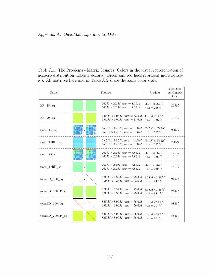
Appendix A. QuadMat Experimental Data
Table A.1: The Problems - Matrix Squares. Colors in the visual representation ofnonzero distribution indicate density. Green and red hues represent more nonze-ros. All matrices here and in Table A.2 share the same color scale.
Name Factors ProductNon-ZeroArithmetic
Ops.
ER_18_sq ×262K × 262K, nnz = 8.39M262K × 262K, nnz = 8.39M
262K × 262Knnz = 268M
269M
ER_20_sq ×1.05M×1.05M , nnz = 33.6M1.05M×1.05M , nnz = 33.6M
1.05M×1.05Mnnz = 1.07G
1.07G
rmat_16_sq ×65.5K × 65.5K, nnz = 1.83M65.5K × 65.5K, nnz = 1.83M
65.5K × 65.5Knnz = 365M
2.15G
rmat_16RP_sq ×65.5K × 65.5K, nnz = 1.83M65.5K × 65.5K, nnz = 1.83M
65.5K × 65.5Knnz = 365M
2.15G
rmat_18_sq ×262K × 262K, nnz = 7.65M262K × 262K, nnz = 7.65M
262K × 262Knnz = 3.04G
16.1G
rmat_18RP_sq ×262K × 262K, nnz = 7.65M262K × 262K, nnz = 7.65M
262K × 262Knnz = 3.04G
16.1G
torus3D_150_sq ×3.38M×3.38M , nnz = 23.6M3.38M×3.38M , nnz = 23.6M
3.38M×3.38Mnnz = 84.4M
246M
torus3D_150RP_sq ×3.38M×3.38M , nnz = 23.6M3.38M×3.38M , nnz = 23.6M
3.38M×3.38Mnnz = 84.4M
246M
torus3D_200_sq ×8.00M×8.00M , nnz = 56.0M8.00M×8.00M , nnz = 56.0M
8.00M×8.00Mnnz = 200M
584M
torus3D_200RP_sq ×8.00M×8.00M , nnz = 56.0M8.00M×8.00M , nnz = 56.0M
8.00M×8.00Mnnz = 200M
584M
195
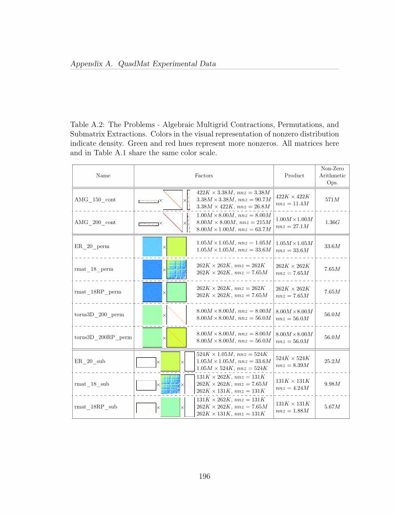
Appendix A. QuadMat Experimental Data
Table A.2: The Problems - Algebraic Multigrid Contractions, Permutations, andSubmatrix Extractions. Colors in the visual representation of nonzero distributionindicate density. Green and red hues represent more nonzeros. All matrices hereand in Table A.1 share the same color scale.
Name Factors ProductNon-ZeroArithmetic
Ops.
AMG_150_cont × ×422K × 3.38M , nnz = 3.38M3.38M×3.38M , nnz = 90.7M3.38M × 422K, nnz = 26.8M
422K × 422Knnz = 11.4M
571M
AMG_200_cont × ×1.00M×8.00M , nnz = 8.00M8.00M × 8.00M , nnz = 215M8.00M×1.00M , nnz = 63.7M
1.00M×1.00Mnnz = 27.1M
1.36G
ER_20_perm ×1.05M×1.05M , nnz = 1.05M1.05M×1.05M , nnz = 33.6M
1.05M×1.05Mnnz = 33.6M
33.6M
rmat_18_perm ×262K × 262K, nnz = 262K262K × 262K, nnz = 7.65M
262K × 262Knnz = 7.65M
7.65M
rmat_18RP_perm ×262K × 262K, nnz = 262K262K × 262K, nnz = 7.65M
262K × 262Knnz = 7.65M
7.65M
torus3D_200_perm ×8.00M×8.00M , nnz = 8.00M8.00M×8.00M , nnz = 56.0M
8.00M×8.00Mnnz = 56.0M
56.0M
torus3D_200RP_perm ×8.00M×8.00M , nnz = 8.00M8.00M×8.00M , nnz = 56.0M
8.00M×8.00Mnnz = 56.0M
56.0M
ER_20_sub × ×524K × 1.05M , nnz = 524K1.05M×1.05M , nnz = 33.6M1.05M × 524K, nnz = 524K
524K × 524Knnz = 8.39M
25.2M
rmat_18_sub × ×131K × 262K, nnz = 131K262K × 262K, nnz = 7.65M262K × 131K, nnz = 131K
131K × 131Knnz = 4.24M
9.98M
rmat_18RP_sub × ×131K × 262K, nnz = 131K262K × 262K, nnz = 7.65M262K × 131K, nnz = 131K
131K × 131Knnz = 1.88M
5.67M
196
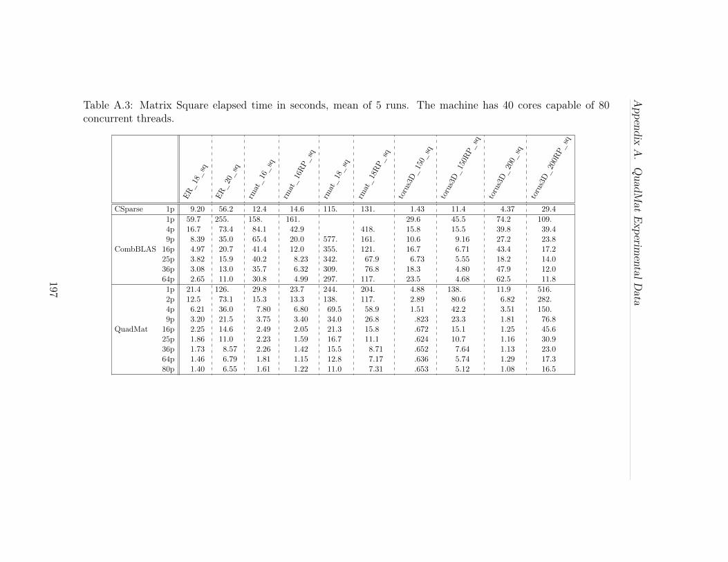
Appendix
A.
QuadM
atE
xperimentalD
ataTable A.3: Matrix Square elapsed time in seconds, mean of 5 runs. The machine has 40 cores capable of 80concurrent threads.
ER_18_sq
ER_20_sq
rmat_16_sq
rmat_16RP_
sq
rmat_18_sq
rmat_18RP_
sq
torus3D_150_
sq
torus3D_150R
P_sq
torus3D_200_
sq
torus3D_200R
P_sq
CSparse 1p 9.20 56.2 12.4 14.6 115. 131. 1.43 11.4 4.37 29.4
CombBLAS
1p 59.7 255. 158. 161. 29.6 45.5 74.2 109.4p 16.7 73.4 84.1 42.9 418. 15.8 15.5 39.8 39.49p 8.39 35.0 65.4 20.0 577. 161. 10.6 9.16 27.2 23.816p 4.97 20.7 41.4 12.0 355. 121. 16.7 6.71 43.4 17.225p 3.82 15.9 40.2 8.23 342. 67.9 6.73 5.55 18.2 14.036p 3.08 13.0 35.7 6.32 309. 76.8 18.3 4.80 47.9 12.064p 2.65 11.0 30.8 4.99 297. 117. 23.5 4.68 62.5 11.8
QuadMat
1p 21.4 126. 29.8 23.7 244. 204. 4.88 138. 11.9 516.2p 12.5 73.1 15.3 13.3 138. 117. 2.89 80.6 6.82 282.4p 6.21 36.0 7.80 6.80 69.5 58.9 1.51 42.2 3.51 150.9p 3.20 21.5 3.75 3.40 34.0 26.8 .823 23.3 1.81 76.816p 2.25 14.6 2.49 2.05 21.3 15.8 .672 15.1 1.25 45.625p 1.86 11.0 2.23 1.59 16.7 11.1 .624 10.7 1.16 30.936p 1.73 8.57 2.26 1.42 15.5 8.71 .652 7.64 1.13 23.064p 1.46 6.79 1.81 1.15 12.8 7.17 .636 5.74 1.29 17.380p 1.40 6.55 1.61 1.22 11.0 7.31 .653 5.12 1.08 16.5
197
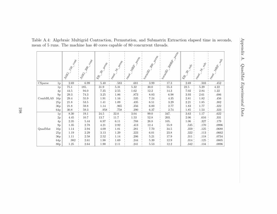
Appendix
A.
QuadM
atE
xperimentalD
ataTable A.4: Algebraic Multigrid Contraction, Permutation, and Submatrix Extraction elapsed time in seconds,mean of 5 runs. The machine has 40 cores capable of 80 concurrent threads.
AMG_150_
cont
AMG_200_
cont
ER_20_perm
rmat_18_perm
rmat_18RP_
perm
torus3D_200_
perm
torus3D_200R
P_perm
ER_20_sub
rmat_18_sub
rmat_18RP_
sub
CSparse 1p 2.69 6.99 5.40 .583 .681 3.99 17.3 2.69 .503 .452
CombBLAS
1p 75.1 185. 31.9 5.31 5.32 30.0 55.3 22.5 5.29 4.224p 44.5 94.0 7.35 2.55 1.62 12.2 14.3 7.02 2.84 1.229p 29.3 74.3 3.25 1.86 .873 8.83 6.98 3.93 2.61 .68616p 29.4 55.9 1.91 1.16 .535 7.24 4.35 2.81 1.82 .45625p 21.8 53.5 1.41 1.09 .435 6.51 3.29 2.21 1.85 .38236p 21.8 59.8 1.14 .965 .356 6.00 2.77 1.83 1.77 .32264p 30.8 59.3 .958 .758 .290 6.37 2.74 1.85 1.53 .323
QuadMat
1p 8.30 19.1 24.5 22.0 3.04 99.0 347. 3.63 1.17 .6222p 4.45 10.7 13.7 11.7 1.53 52.8 203. 2.06 .616 .3314p 2.35 5.44 6.97 6.11 .788 26.8 105. 1.06 .327 .1799p 1.35 2.78 4.21 2.92 .413 12.4 55.9 .535 .170 .099616p 1.14 2.94 4.09 1.81 .281 7.70 34.5 .359 .125 .068825p 1.19 2.29 3.13 1.29 .223 6.01 23.8 .322 .113 .066236p 1.11 2.58 2.52 1.14 .206 5.21 17.9 .311 .118 .073464p .982 2.61 1.98 1.69 .244 5.39 12.9 .314 .125 .080580p 1.25 2.64 1.90 2.11 .241 5.53 12.2 .342 .134 .0896
198
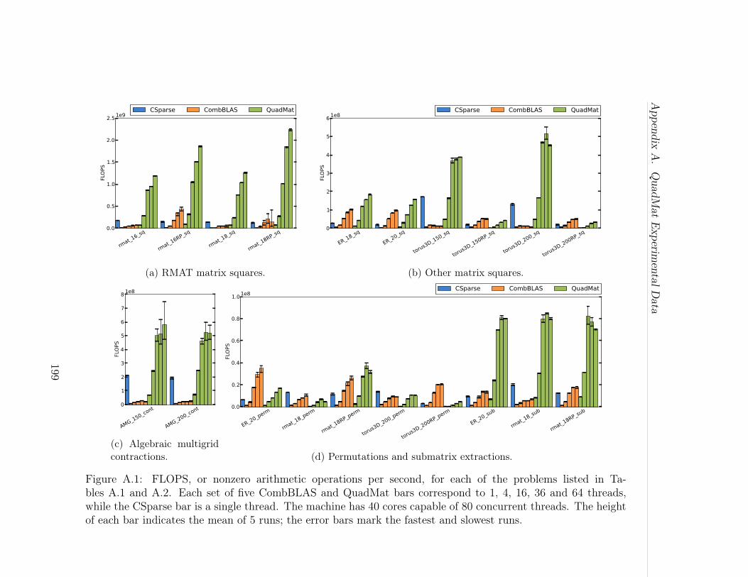
Appendix
A.
QuadM
atE
xperimentalD
ata
rmat_
16_sq
rmat_
16RP_sq
rmat_
18_sq
rmat_
18RP_sq
0.0
0.5
1.0
1.5
2.0
2.5
FLOPS
1e9CSparse CombBLAS QuadMat
(a) RMAT matrix squares.
ER_18
_sq
ER_20
_sq
torus3
D_150_s
q
torus3
D_150R
P_sq
torus3
D_200_s
q
torus3
D_200R
P_sq
0
1
2
3
4
5
6
FLO
PS
1e8CSparse CombBLAS QuadMat
(b) Other matrix squares.
AMG_150_c
ont
AMG_200_c
ont
0
1
2
3
4
5
6
7
8
FLOPS
1e8
(c) Algebraic multigridcontractions.
ER_20
_perm
rmat_
18_pe
rm
rmat_
18RP_pe
rm
torus3
D_200_p
erm
torus3
D_200RP_p
erm
ER_20
_sub
rmat_
18_su
b
rmat_
18RP_su
b0.0
0.2
0.4
0.6
0.8
1.0
FLOPS
1e8CSparse CombBLAS QuadMat
(d) Permutations and submatrix extractions.
Figure A.1: FLOPS, or nonzero arithmetic operations per second, for each of the problems listed in Ta-bles A.1 and A.2. Each set of five CombBLAS and QuadMat bars correspond to 1, 4, 16, 36 and 64 threads,while the CSparse bar is a single thread. The machine has 40 cores capable of 80 concurrent threads. The heightof each bar indicates the mean of 5 runs; the error bars mark the fastest and slowest runs.
199
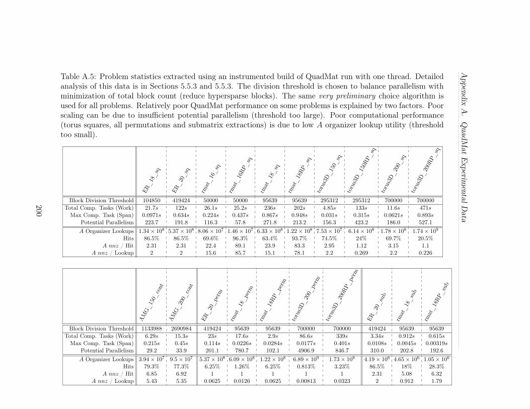
Appendix
A.
QuadM
atE
xperimentalD
ataTable A.5: Problem statistics extracted using an instrumented build of QuadMat run with one thread. Detailedanalysis of this data is in Sections 5.5.3 and 5.5.3. The division threshold is chosen to balance parallelism withminimization of total block count (reduce hypersparse blocks). The same very preliminary choice algorithm isused for all problems. Relatively poor QuadMat performance on some problems is explained by two factors. Poorscaling can be due to insufficient potential parallelism (threshold too large). Poor computational performance(torus squares, all permutations and submatrix extractions) is due to low A organizer lookup utility (thresholdtoo small).
ER_18_sq
ER_20_sq
rmat_16_sq
rmat_16RP_
sq
rmat_18_sq
rmat_18RP_
sq
torus3D_150_
sq
torus3D_150R
P_sq
torus3D_200_
sq
torus3D_200R
P_sq
Block Division Threshold 104850 419424 50000 50000 95639 95639 295312 295312 700000 700000
Total Comp. Tasks (Work) 21.7s 122s 26.1s 25.2s 236s 202s 4.85s 133s 11.6s 471sMax Comp. Task (Span) 0.0971s 0.634s 0.224s 0.437s 0.867s 0.948s 0.031s 0.315s 0.0621s 0.893s
Potential Parallelism 223.7 191.8 116.3 57.8 271.8 213.2 156.3 423.2 186.0 527.1
A Organizer Lookups 1.34× 10⁸ 5.37× 10⁸ 8.06× 10⁷ 1.46× 10⁷ 6.33× 10⁸ 1.22× 10⁸ 7.53× 10⁷ 6.14× 10⁸ 1.78× 10⁸ 1.74× 10⁹
Hits 86.5% 86.5% 69.6% 96.3% 63.4% 93.7% 74.5% 24% 69.7% 20.5%A nnz / Hit 2.31 2.31 22.4 89.1 23.9 83.3 2.95 1.12 3.15 1.1
A nnz / Lookup 2 2 15.6 85.7 15.1 78.1 2.2 0.269 2.2 0.226
AMG_150_
cont
AMG_200_
cont
ER_20_perm
rmat_18_perm
rmat_18RP_
perm
torus3D_200_
perm
torus3D_200R
P_perm
ER_20_sub
rmat_18_sub
rmat_18RP_
sub
Block Division Threshold 1133988 2690984 419424 95639 95639 700000 700000 419424 95639 95639
Total Comp. Tasks (Work) 6.29s 15.3s 23s 17.6s 2.9s 86.6s 339s 3.34s 0.912s 0.615sMax Comp. Task (Span) 0.215s 0.45s 0.114s 0.0226s 0.0284s 0.0177s 0.401s 0.0108s 0.0045s 0.00319s
Potential Parallelism 29.2 33.9 201.1 780.7 102.1 4906.9 846.7 310.0 202.8 192.6
A Organizer Lookups 3.94× 10⁷ 9.5× 10⁷ 5.37× 10⁸ 6.09× 10⁸ 1.22× 10⁸ 6.89× 10⁹ 1.73× 10⁹ 4.19× 10⁶ 4.65× 10⁶ 1.05× 10⁶
Hits 79.3% 77.3% 6.25% 1.26% 6.25% 0.813% 3.23% 86.5% 18% 28.3%A nnz / Hit 6.85 6.92 1 1 1 1 1 2.31 5.08 6.32
A nnz / Lookup 5.43 5.35 0.0625 0.0126 0.0625 0.00813 0.0323 2 0.912 1.79
200
Appendix B
Systems
The experimental results presented in this work have been conducted on severalmachines. They are described here.
B.1 NeumannNeumann is a shared memory machine composed of eight quad-core AMD
Opteron 8378 processors. 16 GB of DRAM is attached to each socket, for a totalof 128 GB in a NUMA arrangement.
Neumann is the CSC lab machine and is located at UCSB.
B.2 MirasolMirasol is a single node platform composed of four Intel Xeon E7-8870 proces-
sors. Each socket has ten cores running at 2.4 GHz, and supports two-way simul-taneous multithreading (20 thread contexts per socket). The cores are connectedto a 30 MB L3 cache via a ring architecture. The sustained stream bandwidth isabout 30 GB/s per socket. The machine has 256 GB 1067 MHz DDR3 RAM.
Mirasol is located at Georgia Tech.
B.3 HopperHopper is a Cray XE6 massively parallel processing (MPP) system, built
from dual-socket 12-core “Magny-Cours” Opteron compute nodes. In reality, eachsocket (multichip module) has two 6-core chips, and so a node can be viewed asa four-chip compute configuration with strong NUMA properties. Each Opteron
201
Appendix B. Systems
chip contains six super-scalar, out-of-order cores capable of completing one (dual-slot) SIMD add and one SIMD multiply per cycle. Additionally, each core hasprivate 64 KB L1 and 512 KB low-latency L2 caches. The six cores on a chip sharea 6MB L3 cache and dual DDR3-1333 memory controllers capable of providingan average STREAM[81] bandwidth of 12GB/s per chip. Each pair of computenodes shares one Gemini network chip, which collectively form a 3D torus.
Hopper is located at NERSC.
B.4 CarverCarver is an IBM iDataPlex system with 400 compute nodes, each node having
two quad-core Intel Nehalem processors. The interconnect is Infiniband.Carver is located at NERSC.
202
Related Documents