Department of Automatic Control Scalable Frequency Control in Electric Power Systems Johan Lindberg

Welcome message from author
This document is posted to help you gain knowledge. Please leave a comment to let me know what you think about it! Share it to your friends and learn new things together.
Transcript

Department of Automatic Control
Scalable Frequency Control in Electric Power Systems
Johan Lindberg

MSc Thesis TFRT-6115 ISSN 0280-5316
Department of Automatic Control Lund University Box 118 SE-221 00 LUND Sweden
© 2020 by Johan Lindberg. All rights reserved. Printed in Sweden by Tryckeriet i E-huset Lund 2020

Abstract
In an effort to curb climate change, the electric power system in many countries istransitioning from fossil fuels to more renewable power sources such as wind. Atthe same time, other countries are decommissioning their old nuclear power, andreplacing it with wind power. When replacing synchronous machines with windpower the inertia in the system is decreased. If nothing is done about this the perfor-mance of electric power grids will deteriorate. For example, the frequency deviationat a disturbance in power balance will increase.
In this thesis the effects of more wind power in the Swedish electric power sys-tem was investigated. This was carried out by building two models of the Swedishelectric power system in Matlab Simulink®. The first model was a one node repre-sentation of the Swedish system, and the second was a two node representation. Forthe two models both today’s system, and a future scenario without nuclear powerwas tested. Simulations with different losses of generation were preformed and theresults examined. The usage of wind turbines for frequency control was investi-gated. To do this, 10% of the power in the wind was curtailed to enable increasedpower output when needed. A controller was introduced for the wind turbine, withthe grid frequency as the measurement signal. This was tested for different amountsof the wind turbines contributing to the frequency control. The stability of the twonode model was also investigated with theory for distributed control. The effects ofreplacing nuclear power with wind power in Sweden was also investigated by simu-lations in the existing Nordic 32 model, implemented in the dynamic power systemsimulation software PSS®E.
The different simulations, and the control theory, showed that if more windpower is being built without controlling the frequency of the grid, the performanceat a disturbance will deteriorate as the inertia in the system is reduced. If wind tur-bines are used for frequency control the performance can be significantly improved,and actually preform better than today’s system (with nuclear power), with no fre-quency control from wind turbines.
3


Acknowledgements
I would like to thank my supervisors Richard Pates, Daniel Karlsson, Olof Samuels-son and Daria Madjidian for helping me with my thesis. I would especially like tothank them for all the comments along the way and always being there when Iwanted to discuss some ideas. I would also like to thank all the people at the De-partment of Automatic Control and at DNV GL who have helped me throughoutthis thesis. Finally, I would like to stress that I have felt very welcomed both at thecontrol department at LTH and at DNV GL and I really appreciate that I have feltlike a part of both teams.
5


Contents
1. Introduction 91.1 General background and energy transition . . . . . . . . . . . . 91.2 Frequency stability and requirements . . . . . . . . . . . . . . . 101.3 Objectives and limitations of this thesis . . . . . . . . . . . . . . 131.4 Outline of the report . . . . . . . . . . . . . . . . . . . . . . . . 14
2. Theoretical background 152.1 Swing equation . . . . . . . . . . . . . . . . . . . . . . . . . . 152.2 Wind power . . . . . . . . . . . . . . . . . . . . . . . . . . . . 202.3 Power grid models . . . . . . . . . . . . . . . . . . . . . . . . . 222.4 Distributed conditions . . . . . . . . . . . . . . . . . . . . . . . 24
3. Method 273.1 Simplified Matlab®and Simulink®models . . . . . . . . . . . . 283.2 Model of generation sources and loads in Matlab® . . . . . . . . 363.3 Linear analysis . . . . . . . . . . . . . . . . . . . . . . . . . . . 443.4 PSS®E model . . . . . . . . . . . . . . . . . . . . . . . . . . . 46
4. Results 544.1 One node Matlab®simulation . . . . . . . . . . . . . . . . . . . 544.2 Two node Matlab®simulation . . . . . . . . . . . . . . . . . . . 624.3 Linear analysis . . . . . . . . . . . . . . . . . . . . . . . . . . . 684.4 PSS®E results . . . . . . . . . . . . . . . . . . . . . . . . . . . 72
5. Discussion 776. Conclusion 817. Future work 82Bibliography 838. Appendix 1 Plots of some of the Simulink®simulations 869. Appendix 2 Matlab®simulations with no backlash 92
9.1 One node model . . . . . . . . . . . . . . . . . . . . . . . . . . 929.2 Two node model . . . . . . . . . . . . . . . . . . . . . . . . . . 98
10. Appendix 3 Complementing PSS®E simulation results 104
7


1Introduction
1.1 General background and energy transition
In an effort to curb climate change, our society is transitioning from an energy sec-tor with high fossil fuel dependency, to a more electrified energy sector, where asubstantial amount of our energy will be provided by wind and solar plants. Thistransition must continue if the goal of stopping climate change is to be achieved[Masson-Delmotte et al., 2018]. Sweden has, for example, set a target that 100% ofelectricity generation should come from renewable sources by 2040 [ENERGY USEIN SWEDEN]. Sweden has barely any electric power production from fossil fuels,but a substantial part comes form nuclear power. In 2019 a total of 64 478 GWh ofelectric energy was generated by nuclear units in Sweden [Elstatistik - Statistik helalandet per månad 2019(xls)]. Nuclear power is greenhouse gas emissions free, butnot considered renewable. If Sweden is to reach 100% renewable electricity produc-tion by 2040, the current nuclear stations must be taken out of service. The currentnuclear units are in many cases reaching the end of their lifetime, and are at the mo-ment planned to all be decommissioned around 2040 [Strålsäkerhatsmyndigheten -Kärnkraft]. At the end of 2019, one of the nuclear station in Ringhals was closed,and another will close at the end of 2020.
One of the main obstacles to this energy transition is the weather-dependentvariability and uncertainty in wind and solar power, leading to the likely imbalancebetween production and consumption at many times. Another problem arises whenthe AC power injected to the electric power grid comes from inverters without anynatural inertia. If there is an unexpected loss of generation or loss of load, thiscould lead to a large decrease or increase in network frequency. Because of this,some nations, e.g. Ireland, have set hard limits on the proportion of the power thatcan be delivered by non-synchronous machines. In Ireland’s case, the System Non-Synchronous Penetration is not allowed to exceed 65% at any time [OperationalConstraints Update 29/03/2019]. However, this is the current limit. It has risen fromlower limits and could potentially continue to rise.
To be able to cope with these unexpected events and to maintain a stable net-work frequency, one approach is to develop a control strategy mimicking the inertia
9

Chapter 1. Introduction
in present day synchronous machines [J. Driesen, 2008]. Alternatively a controlstrategy that can keep the grid within present day frequency limits in a situationwith low inertia is needed. With such a control strategy, it could be possible to nothave any of the current limits on the use of renewable energy sources based oninverter injected power. Alternatively, to have significantly higher limits than thecurrent hard limits, without losing the robustness these present limits are set up tomaintain.
Conventionally wind turbines produce the maximum power possible and injectit into the system. If the goal of 100% renewable electric power is to be achievedin Sweden a large part of the power will come from wind power. With wind powerbeing a large part of the non-synchronous generation the frequency control wouldbenefit if they could contribute. If a wind turbine is going to be able to contributeto frequency control, some of the power in the wind must be curtailed in normaloperation to allow for more power to be produced when needed [Elorza et al., 2019].
1.2 Frequency stability and requirements
Frequency stability is the ability to maintain a stable AC frequency in a power gridin the event of an extreme disturbance between the balance of production and con-sumption [Kundur, 1994]. An extreme disturbance is, for example, the loss of an theentire capacity of a generating station, or the loss of all lines coming from a gener-ating station, switching station or substation. A major disturbance can also arise ifthere is a significant loss of load from a large load centre [Kundur, 1994].
The nominal frequency in Sweden and the Nordic power grid is 50 Hz, andthe normal frequency band is 50± 0.1 Hz. The frequency quality in Sweden andthe Nordic synchronous system has deteriorated in the last years. This has beenindicated by more minutes outside the normal frequency band than a couple of yearsago. The ambition is that the frequency should not be outside it more than a total of10 000 minutes per year, which corresponds to 1.9% of the time [Robert Eriksson,2017].
The Swedish electric power grid and the Nordic synchronoussystemThe Swedish power grid is a part of the Nordic synchronous system. The Nordicsynchronous system consists of Sweden, Norway, Finland and eastern Denmark(Zealand, Bornholm and the islands south of Zealand). The Swedish TSO (trans-mission system operator) Svenska kraftnät is responsible for the operation of theSwedish power grid. The other countries in the Nordic synchronous area have theirown TSOs and together they are responsible for the operation of the Nordic syn-chronous system. The Nordic synchronous system is connected to the continentalEuropean synchronous system, the Baltic synchronous system and from 2021 the
10
1.2 Frequency stability and requirements
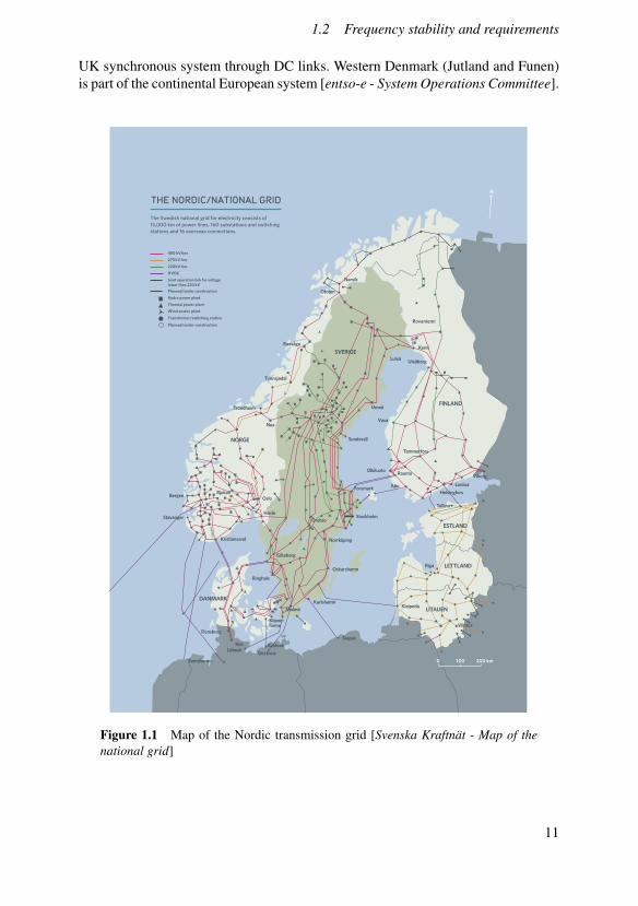
UK synchronous system through DC links. Western Denmark (Jutland and Funen)is part of the continental European system [entso-e - System Operations Committee].
(300
kV
)
R tock
Ringhals
K pe -ham
Göteborg
almöKarlshamn
Norrköping
Örebro
Oskarshamn
HasleStavanger
Bergen RjukanOslo
Stockholm
Nea
Trondheim
Tunnsjødal
Umeå
Sundsvall
Røssåga
Ofoten
Narvik
SVERIGE
NORGE
FINLAND
Loviisa
OlkiluotoViborg
Kristiansand
Rauma
Forsmark
0 100 200 km
Luleå
Vasa
Tammerfors
Kemi
Uleåborg
KielLübeck
Slupsk
Eemshaven
N
Klaipeda
Riga
Vilnius
ESTLAND
Tallinn
LETTLAND
Helsingfors
Flensburg
DANMARK
Åbo
Rovaniemi
LITAUEN
os
nn
M
ö
Güstrow
THE NORDIC/NATIONAL GRID
15,000 km of power lines, 160 substations and switchingThe Swedish national grid for electricity consists of
stations and 16 overseas connections.
00 kV line
2 5 kV line
20 kV line
VDC
4
7
2
H
Joint operation link for voltagelower than 220 kVPlanned/under construction
Hydro power plant
Thermal power plant
Planned/under construction
Transformer/switching station
Wind power plant
Figure 1.1 Map of the Nordic transmission grid [Svenska Kraftnät - Map of thenational grid]
11

Chapter 1. Introduction
The Swedish system is split up into 4 so called elec-tricity areas, with different prices for trading electricity.Electricity area 1 (Luleå) is the northernmost, electricityarea 2 (Sundsvall) follows after, and then electricity area3 (Stockholm) and 4 (Malmö) are in the south [SvenskaKraftnät - The control room]. A rough sketch of the ar-eas can be seen to the right [Storuman enegi AB - Omjämförpriser]. Most of the hydro power in Sweden islocated in area 1 and 2, and the two areas produce moreelectric power than they consume. Area 3 has all the nu-clear power, but since it has the highest consumption itis a net consumer. Area 4 has little production, and isa net consumer of electric power [Elstatistik - Statistikper elområde och timme, 2019(xls)]. Wind power gen-eration is spread out in all areas, but with most of thegeneration coming from the 2 geographically largest ar-eas (2 and 3). Because of the imbalance between whereelectric power is generated and where it is consumed, anextensive transmission network is needed. In Figure 1.1 the Swedish transmissionnetwork can be seen.
The frequency control in the Nordic synchronous system is organised in a setof terms. These terms are; FFR (Fast Frequency Reserve), FCR-N (Frequency Con-tainment Reserve Normal), FCR-D (Frequency Containment Reserve Disturbed),aFRR (automatic Frequency Restoration Reserve) and mFRR (manual FrequencyRestoration Reserve). The FRR is an automatic support to handle fast frequencychanges in low inertia situations. The FCR-N is an automatic power support to sta-bilise the frequency for small differences in consumption and production of electricpower. It is automatically activated within a 0.1 Hz deviation from the nominal fre-quency, has a volume of 200 MW for Sweden and should be activated to 63% within1 minute and 100% within 3 minutes. The FCR-D is also an automatic power sup-port that should stabilize the frequency at disturbances. It is activated automaticallyif the frequency goes below 49.90 Hz, has a volume of 400 MW for Sweden andshould be activated to 50% within 5 seconds after the frequency is below 49.90 Hzand to 100% within 30 seconds. The aFFR is an automatic power support that resetsthe frequency to 50 Hz by changing power output from the generators. It is acti-vated by an automatic central control signal, has a volume of 150 MW and shouldbe 100% activated within 2 minutes if needed. Finally, the mFRR has the samefunction as the aFRR, but is activated manually by demand from Svenska kraftnät,to relieve all the automatically activated frequency control. From the demand fromSvenska kraftnät the mFRR should be activated within 15 minutes. How this is doneand which generators is activated is decided by trade and market agreements [Sven-ska Kraftnät - Information om stödtjänster] [Svenska Kraftnät - Översiktlig kravbildför reserver].
12

1.3 Objectives and limitations of this thesis
1.3 Objectives and limitations of this thesis
The objective of this thesis was to investigate the frequency behaviour after a majorloss of generation for different amounts of frequency control performed by wind tur-bines. The wind turbines should only act on the signals in that place, i.e no commu-nications between different parts of the grid should be used. This was done by sim-ulation of a fault in several models of the Swedish power grid. The first model usedwas a one node model implemented in Matlab Simulink®. The second model usedin this thesis was a two node model, also implemented in Matlab Simulink®. Thethird most sophisticated model used was a pre-implemented model called Nordic32, with 32 transmission nodes. The Nordic 32 model was implemented in a dy-namic power system simulation software called PSS®E.
The one and two nodes models were highly simplified models based on his-toric data of the Swedish power system. The aim of these models was not to createa perfect representation of the Swedish electric power system, but rather to createmodels that were reasonable to investigate tendencies in the frequency behaviour,with different amounts of frequency control by wind turbines. This thesis is onlyconceptual. Therefore the results should not be taken as predictions about the actualSwedish or Nordic power system, but rather as indications of what might happen,and what might be the effects of using wind turbines for frequency control. A sig-nificant limitation in the Simulink®simulations was that only the Swedish powersystem was considered, despite its close connection to the Nordic synchronous sys-tem. Since this work only is conceptual it will not express the control of frequencyin terms of FFR, FCR-N, FCR-D, aFRR or mFRR.
Both in the Matlab®simulations and in the PSS®E simulation a present case anda future scenario was investigated. In the future scenario in the Matlab®and in thePSS®E simulation no storage was considered and the load was equal to today’s situ-ation. There are concerns about lower inertia, and also about a possible lower load-frequency dependency in the future electric power system. Only the effect of lowerinertia was investigated in this thesis and not a lower load frequency dependency.Another limitation in the future scenario in this thesis was that no transmissionlines were altered in the Nordic 32 model. Further restrictions in this report is thatonly the initial, automatic frequency recovery is considered, and no consideration istaken to the economic aspects of the operations of a power grid or generators.
From the two node Simulink®model a linear analysis was performed inMatlab®to investigate if any insight could be obtained by checking stability con-ditions for distributed control.
13

Chapter 1. Introduction
1.4 Outline of the report
• In Chapter 2 the theories and mathematical formulas needed for the rest ofthe report are presented. This chapter could either be read before reading thefollowing chapters, or be used as a look up for the theory when reading theother chapters.
• Chapter 3 explains how the different models were obtained and how the sim-ulations were performed.
• In Chapter 4 the results of the simulations are presented and briefly com-mented.
• Chapter 5 then reflects on the result and its implications.
• In the appendices some more results, relating to the ones in Chapter 4 arepresented. These results were not considered core results, and were omittedin Chapter 4 to not make it too cramped.
14

2Theoretical background
In this chapter the theoretical background needed for the rest of the report will bepresented. It will cover the impact of inertia on the frequency in a power grid, andexplain how a wind turbine works. Furthermore, this chapter will present the powergrid modelling used in the thesis and the distributed control theory that was used toinvestigate stability.
2.1 Swing equation
Swing equation for one synchronous machineFor a synchronous machine the swing equation can be derived as follows from New-tons second law
Jd2θ(t)
dt2 = Tm(t)−Te(t). (2.1)
In the above equation, θ is the rotor angle of the synchronous machine in radians,Tm is the mechanical torque, minus mechanical losses, being applied by the primemover, and Te the electric torque arising from the electro-magnetic coupling withthe grid. Multiplying both sides with the angular velocity ω of the machine we get
Jω(t)d2θ(t)
dt2 = Jω(t)dω(t)
dt= (Tm(t)−Te(t))ω(t) = Pm(t)−Pe(t). (2.2)
It is conventional to use Hz rather than radians per second and per units (pu) quan-tities, so we introduce ω(t) = 2π f (t) and the inertia constant
H =stored kinetic energy at synchronous speed
generator VA rating=
12 Jω2
0
Srated. (2.3)
Here ω0 is the nominal (steady state) angular frequency. Equation (2.2) can be trans-formed to
15

Chapter 2. Theoretical background
2Hω2
0ω(t)
dω(t)dt
=2Hf 20
f (t)d f (t)
dt=
Pm(t)−Pe(t)Srated
= Pm,pu(t)−Pe,pu(t), (2.4)
where f0 is the nominal (steady state) frequency in Hz, Pm,pu(t) and Pe,pu(t) are themechanical power and electric power in per unit. Linearising around the steady statefrequency f0 where f (t) d f (t)
d ≈ f0∆ fdt and only looking at the deviation from f0 with
∆ f (t) = f (t)− f0 gives the following linearised equation
2Hf0
d∆ f (t)dt
= Pm,pu(t)−Pe,pu(t). (2.5)
Swing equation for one node with several synchronousmachines.If multiple synchronous machines are connected at the same bus, each can be mod-elled as in the single machine case.
2Hi
f0
d∆ fi(t)dt
= Pm,pu,i(t)−Pe,pu,i(t) (2.6)
Furthermore, for many generators to be able to produce power for the loads in a busthey must rotate with the same frequency. Also, it can be assumed that all generatorsin a bus swing coherently (the angular velocities of the rotors of the different ma-chines are identical).1 This means that ∆ fi(t)
dt are the same for all i [Robert Eriksson,2017]. Then all the powers can be added in the following way
1 Assume that all generators are rotating with the same frequency at a time instance t0 and that ingenerator i Pm,pu,i(t0) = Pe,pu,i(t0). In that case d∆ fi(t0)
dt = 0. If the mechanical power of the generator
i suddenly decreases at time t1 by a small amount, when d∆ fi(t1)dt < 0. This will lead to that ∆ fi(t)
decreases for this specific generator. Assume further that the frequency of all other generators in thebus are not affected. The phase of generator i in relation to the other generators in the bus, who’sphases are the same since they are all rotating with the same nominal frequency, is given by
∆θi(t) =∫ t
t12π∆ fi(t)dt. (2.7)
After t1 the phase of generator i is falling behind the others. When this happens the electric torqueacting on generator i will decrease due to that the electromagnetic forces in the generator are smallerwhen the rotor of the geneator is lagging the grid phase angle [J. Duncan Glover, 2010]. This issometimes referred to as the damping torque. Since the electric power is proportional to the torquethis too will decrease. Because of this, if ∆θi < 0 the electric power acting on generator i will beless than the mechanical power. Then d∆ fi(t1)
dt > 0 and both ∆ fi(t) and ∆θi(t) will increase until theyreach the same value as as the other generators in the bus i.e. 0. If instead there would be a smallincrease in mechanical power, the same dynamics would happen but with opposite signs.
16

2.1 Swing equation
∑i
2Hi
f0
d∆ fi(t)dt
= ∑i(Pm,pu,i(t)−Pe,pu,i(t))
⇔ 2Hf0
d∆ f (t)dt
= Pm,pu,(t)−Pe,pu,(t). (2.8)
where
H = ∑i
Hi and Pm,pu,(t)−Pe,pu,(t) = ∑i(Pm,pu,i(t)−Pe,pu,i(t)). (2.9)
In this way all generators in a bus are modelled as one large generator. Theelectric power produced by the generators in a bus is consumed by loads connectedto that bus. The electric power consumed can be assumed to be non frequency de-pendent, to a large extent. However, often a part of the load is frequency depen-dent. This can for example be AC motors connected to the grid with electric powerconsumption proportional to the speed of rotation. Given this, the per unit electricpower can be divided into one constant part and one proportional part dependingon the frequency deviation from the stationary frequency, just like is done by Sven-ska kraftnät in [Robert Eriksson, 2017] Pe,pu(t) = P0
e,pu + k∆ f (t). By inserting thisequation (2.8) becomes
2Hf0
d∆ f (t)dt
= Pm,pu,(t)−P0e,pu,− k∆ f (t). (2.10)
In a one node system the transfer function from difference in power to deviationfrom the stationary frequency becomes
∆ f (s) =f0
2Hs+ k f0∆Ppu(s) =
f0/Srated
2Hs+ k f0∆P(s). (2.11)
In the above (in a slight abuse of notation), ∆ f (s), ∆Ppu(s) and ∆P(s) are the Laplaceversions of ∆ f (t), ∆Ppu(t) and ∆P(t). Here ∆Ppu(t) = Pm,pu,(t)−P0
e,pu, and ∆P(t)is the same function without per unit base. The left part of equation (2.11) is thetransfer function from per unit power deviation to frequency deviation. This is thesame model that is used by Svenska kraftnät in [Robert Eriksson, 2017] and [MikkoKuivaniemi, 2017]. The right part of equation (2.11) is the same equation withoutper unit base. This is a transfer function from a power deviation in Watts to fre-quency deviation in Hz, from the linearisation point (nominal operation point).
Frequency response and inertiaIn synchronous machines connected to the electric power grid there are a lot ofheavy parts rotating at high speed. The inertia constant is defined as the storedkinetic energy divided by the rated power. It is a measurement of how long the
17

Chapter 2. Theoretical background
kinetic energy from these rotating masses could be used to procure the rated electricpower, before all kinetic energy is used up. In a bus with many generators the inertiaconstant can be interpreted as the time the kinetic energy stored in all the rotatinggenerators and turbines can deliver the total power produced from the bus, if no newmechanical power was added to any of the turbines in that bus.
Equation (2.11) is derived from the balance between the mechanical power ap-plied to a generator, and the electric taken out to the grid. The same equation holdswhen looking at frequency deviation as a result of power imbalance between elec-tric power produced by a group of generators in a node, and the electric powerconsumed by the loads in that node. A common way to investigate the frequencybehaviour is to look at the step response, for a step in power. The step is defined as∆P(t) = 0 for t < 0. At time t = 0 ∆P(t) takes a step of height ∆Pf inal and remainsat this value. This corresponds to the loss of a load if ∆P(t) is a positive step. If in-stead a loss of generation would occur this corresponds to a negative step in ∆P(t).From equation (2.11) it can be seen that if more power is produced than consumedin the grid, the frequency will go up, and if more power is consumed than produced,the frequency will go down. The most severe case in an electric grid is often theloss of a big generator unit. This is because the largest generator is often larger thanthe largest load unit in a grid. If a loss of generation occurs then the frequency willdecrease. If nothing is done to compensate for the loss of generation, by the finalvalue theorem, the frequency deviation from f0 will be [Hägglund, 2019]:
∆ f f inal ≈1
Sratedk∆Pf inal . (2.12)
This is because if the load is frequency dependent with dependency k a new equi-librium will eventually occur. Since equation (2.11) is the result of a linearisationaround f0 equation (2.12) is only approximate. Insight to the initial behaviour canbe obtained from the initial value theorem. In particular [Hägglund, 2019],
d∆ f (0)dt
=f0/Srated
2H∆Pf inal . (2.13)
Remember that ∆Pf inal is the power difference without control effort. The conclu-sion from this is that the larger value of H the less steep slope of the initial trajectoryof the frequency responses. A large inertia gives the control strategies time to acti-vate the generators with frequency control resources that are still on-line. In Table2.1 the inertia constant for different types of generators are listed [Ørum et al.,2015].
From Table 2.1, it is clear that the inertia will decrease in a future energy systemwith nuclear generation replaced by wind and solar production. There exists severaltypes of wind turbines, and the inertia listed in Table 2.1 is for the type described inthe coming wind power section. In Figure 2.1 the frequency response of three simplepower systems with the same rated power but different inertia are plotted. The plotsare for the same loss of generation. In these simple systems a simple controller is
18

2.1 Swing equation
Table 2.1 Inertia constants of different types of generators
Generator type H [s]Nuclear 6.3
Other thermal 4Hydro 3Wind 0Solar 0
acting on the generators that are still in operation to recover the lost power. In theright picture in Figure 2.1 the initial derivative, calculated from equation (2.13), areplotted for the three step responses.
0 5 10 15 20 25 30−0.5
−0.25
0
Time s
freq
uenc
yde
viat
ion
H=3H=5H=7
−1 0 1 2 3 4
−0.2
−0.1
0
Time s
H=3H=5H=7
Figure 2.1 Frequency response of a simple system with different inertia constants.
The lowest value of the frequency during a loss of generation is called the fre-quency nadir. In Figure 2.1 it can be seen that a lower inertia in the system gives alower frequency nadir.
Droop controlIn the event of a loss of a generator, the remaining generators must compensatefor the unit lost. It is desirable that the remaining units that can change their elec-tric power output to compensate for the lost generator, according to their sizes. Inthis way the burden is split evenly. A common way to do this is by droop control[Kundur, 1994]. The droop constant epis defined by
ep :=∆ f/ f0
∆Pgenerator/Sn,generator. (2.14)
The droop constant determines how much a generator with droop control willchange its power output (∆Pgenerator) for a given frequency deviation, form the nom-
19

Chapter 2. Theoretical background
inal frequency. The droop constant is included in the control as an internal feedback,restricting the input to the controller, and at the event of a lost generator the gener-ators with droop control will only try to compensate relative to its rated power. Tosee the structure of the droop control see Figure 3.4, in the Method Chapter. Often aPI controller is used for controlling the frequency. The PI controller is acting on thelinearised system, meaning that for no frequency deviation the PI controller outputis zero, when the frequency deviates from f0 the PI controller sends a signal to addpower to the constant, scheduled power. The droop internal feedback has the effectof limiting the PI controller, effectively limiting the DC gain to 1/ep. This gives astationary error in the initial frequency control. It is common to set the droop con-stant in the range 2-12% [Robert Eriksson, 2017]. The droop constant is a relativevalue of how much the generator output changes in relation to frequency deviation.For example, if ep = 5%, then for a loss of 5% of the frequency (5% of 50 Hz is2.5 Hz) a generator with droop control for frequency control would try to increaseits power output by 100%. Or, at a deviation of 0.5 Hz from the nominal frequencygenerators with droop control would increase their power outputs by 20%. Sincethere are dynamics in the generator and in the power system this is what wouldhappen after the frequency nadir in the new steady state with a frequency differentfrom the nominal frequency. If there was no droop in the system, fast respondinggenerators would compensate for all the lost generation before the slower ones hadtime to act. Note that a system with droop control at its generators will not auto-matically return to the nominal frequency after a loss of generation. After the auto-matic response, secondary frequency control can be activated, either automaticallyor manually, to compensate for the lost generator. The way this is done is decidedby previous agreements and trade deals [Svenska kraftnät - Störningsreserven]. Anew generator is started or already on-line generators get a new scheduled poweroutputs. This will eventually bring the frequency back to the operational 50 Hz andtake over the extra production from the generators that automatically respondeddirectly after the fault.
2.2 Wind power
Available wind powerAssuming a constant wind speed u the power of the wind Pw in a cross section ofthe atmosphere is given by [J.F Manwell, 2009]
Pw(u) =12
ρAu3. (2.15)
In this equation ρ is the density of the air, u is the wind speed and A is the crosssection area, perpendicular to the the wind direction. This model assumed that thewind speed is constant through the whole cross section. In reality the wind speed isoften higher further from the ground [J.F Manwell, 2009].
20

2.2 Wind power
The portion of the power that a wind turbine can extract from the power in thewind is denoted by the power coefficient CP = Power produced by the wind turbine
Available power in the wind = Pwt (u)Pw(u)
The theoretical maximum power that a turbine can extract is given by the Betz limit,named after the person who first derived it. The Betz limit can be calculated to beCP,max = 16/27≈ 0.6. This theoretical maximum power coefficient assumes that thewhole area is covered by an infinite amount of blades with zero drag and frictioni.e. an actuator disk [J.F Manwell, 2009]. If one instead looks at a 3 blade windturbine with drag taken into account the theoretical CP,max is slightly above 0.5 andis very dependent on the ratio of lift vs drag. [J.F Manwell, 2009]. CP,max of thewind turbine used throughout this thesis is 0.4866.
Operation of a wind turbineIn this section the operation of an upwind, three bladed, horizontal axis, variablespeed and pitch controlled wind turbine with a gearbox and an inverter for connec-tion to the power grid will be explained. This type of turbine is the most commonlyused for large scale wind power generation.
The operation of a wind turbine can be divided into four different regions ofoperation. At very low wind speeds the friction and other resistances are higherthan the power a turbine can extract from the wind. In this situation the turbine isturned off and doesn’t produce any electric power. This is often referred to as region1 [J.F Manwell, 2009]. In region 1 the mechanical brakes are activated to make surethat the turbine doesn’t move for gusts in the wind.
After the cut-in wind speed, the brakes are released and the turbine controlleris designed to try to maximise the power output from the wind turbine. If the windcontinues to increase, the wind turbine will eventually reach its rated power. Thisis the power its generator and mechanical components were designed to be able totake. The wind speed at which the wind turbine reaches its rated power is calledthe rated wind speed. When a wind turbine operates between cut-in and rated windspeeds it is said to be operating in region 2 [J.F Manwell, 2009]. In this operatingregion the power output varies with the wind speed.
If the wind is above the rated wind speed the turbine could theoretically producemore electric power than the generator and shaft can manage. In steady state, thetorque from the rotor side of the generator and the electric torque from the grid mustbe equal. To make sure that the torques on the shaft and generator aren’t too largethe blades are pitched to let some of the wind past the blades so that the mechanicaltorque doesn’t exceed the rated torque. This region of operation is often referred toas region 3. In a modern wind turbine, the controller tries to maintain the electricpower output to the rated power, by ’pitching to feather’ to not catch all the wind itpotentially could. ’Pitch to feather’ means turning the blades a little more upwindthan the ideal for caching all the power in the wind. Another way is to ’pitch tostall’, which means that the blades are pitched with an angle more in line with therotation, than the angle catching the most wind power. This would lead to higher
21
Chapter 2. Theoretical background
flap-wise torques compared to pitch to feather, and therefore pitch to feather is thepredominant technique used [J.F Manwell, 2009].
If the wind speed is above the cut-out speed the wind turbine is shut down. Thisis due to safety and to make sure that the turbines don’t break down from too highforces and stresses. This region is often referred to as region 4 [J.F Manwell, 2009].In this region, the turbine is facing upwind and the blades are pitched to not takeany power from the wind i.e. roughly 90 degrees. The pitching angles are activelycontrolled to be able to withstand sudden gusts. Together with the pitching of theblades, the breaks are also activated to make sure that the turbine doesn’t start torotate. These two procedures make sure that the turbine is standing still in highwinds, and doesn’t produce any electric power.
2.3 Power grid models
National and international networks for power transmission are generally threephase AC networks [Kundur, 1994] [J. Duncan Glover, 2010]. However, when per-forming power flow calculations three phase networks are often represented by asingle line equivalent [J. Duncan Glover, 2010]. Once the single line flows havebeen determined, one can then transform the results back to the actual voltages, cur-rents and phases in the three phase grid. However, when doing large scale powerflow calculations the single line equivalent is often the only one used. When oneis designing the individual components and generators the conversion back to thethree phase system is more important. In this report only the single line equivalentwill be used. The reason for this is that the loss of a generator is a symmetric faultaffecting the three phases equally.
Steady state power flow solutionsOnce a single line equivalent network is obtained, one often wants to know thesteady state power flow in the network. In order to specify the steady state flows,four variables per bus must be determined. Typically at each bus two of these quan-tities are specified. The objective of the power flow analysis is to find the remain-ing variables at each bus, subject to transmission line constraints. The quantities inquestion are active power (P), reactive power (Q), voltage (V) and phase angle (φ ).
In power networks, three types of buses are considered:
• PQ-bus
• PV-bus
• Swing-bus/Slack-bus
The PQ-bus is often called load bus and has a specified active and reactive powerexchange with the network. The PV-bus is often called generator bus and has fixed
22

2.3 Power grid models
active power injection and fixed voltage. These are, as the name suggests, connectedto a generator with fixed voltage and specified active power generation. The swing-bus is usually chosen as the largest generator bus. This bus has fixed voltage and afixed phase angle (often set to zero). The angles of all other buses are then definedin relation to this swing-bus [J. Duncan Glover, 2010]. The swing-bus can gener-ate/absorb active and reactive power to make sure that there is a balance in electricpower. In a network, lines and transformers often have an impact on the voltagesand phases in the buses, and active and reactive power exchange between them. Theline and transformer parameters determine how they will affect the system for agiven situation. Therefore, the power flow solution is not trivial.
To get the steady-state power flow an iterative numerical solution is often used.In the PV-buses active power and voltage are known while reactive power and thephase angle are unknown. These unknown values are set to an initial guess, or tothe previously calculated values in the optimisation iteration. In the PQ-buses activeand reactive power are known and angle and voltages are guessed in a similar wayto the PV-buses. The swing-bus has its phase angle set to zero and voltage set to thespecified voltage, while active and reactive power are guessed. Then an optimisa-tion method, such as the Newton-Rapson method or an SDP relaxation technique isused to determine the unknown variables. If the Newton-Rapson method is used ititeratively get a better and better guess for the next iteration, if the first guess wasclose enough to the solution. The SDP relaxation gets the correct variables in thefirst calculation, if it is tight. Once the difference in values between two iterationsare below a pre-set threshold the iterations stop and the values in the last iterationare considered to be the solution to the power flow [J. Duncan Glover, 2010]. Asolution to this optimisation is the steady-state power flow with a consistent set ofphase angles, voltages and reactive and active power. This solution can then be usedas a starting point for a dynamic simulation.
Transmission linesThe active and reactive power delivered to the receiving end of a transmission lineare given by the following equations [J. Duncan Glover, 2010]:
PR =VRVS
Z′cos(θZ−φ)− AV 2
RZ′
cos(θZ−θA)
QR =VRVS
Z′sin(θZ−φ)− AV 2
RZ′
sin(θZ−θA) (2.16)
Here VR and VS is the voltage magnitude of the bus at the receiving respectivelysending end of the line. The variable φ is the difference in voltage phase anglebetween the receiving and sending end voltages. Z′ and A are line parameter con-stants that arise from the line resistance, conductance, inductance and capacitance.Z′ and A are here real numbers and θZ and θA are their associated phasor angles,
23

Chapter 2. Theoretical background
see [J. Duncan Glover, 2010] chapter 5. A normal approximation is to look at alossless line. For high-voltage transmission this often gives a good approximation,especially when only looking at active power and frequency variation. For a losslessline Z′ = X ′, θA = 0◦, θZ = 90◦ . Thus, equation (2.16) for active power becomes:
PR =VRVS
X ′cos(90◦−φ)− AV 2
RX ′
cos(90◦) =VRVS
X ′sin(φ) = Pmax · sin(φ) (2.17)
Here X ′ is the line reactance. In a lossless line the maximum power transmittedis when the phase difference between the sending and receiving nodes is 90◦. Ifthe phase angle would be larger than 90◦ the power transmitted would be smallerthan the one at 90◦ and the system would become unstable. Due to the instabilityof the system once the phase angle becomes more than 90◦, a transmission line isalways operated at a phase angle smaller than 90◦ with margins to the maximumtransmitted power [Kundur, 1994]. Since the line is lossless the received and sentactive power are equal.
2.4 Distributed conditions
When determining the stability of a system with feedback the Nyquist curve ofthe open loop (system without feedback) is often studied. In Figure 2.2 a simpleblock diagram is shown, with constant negative feedback k. If the open loop transferfunction is marginally stable, i.e. all poles are in the left half plane and any poleson the imaginary axis are simple (not more than one in the same location), thenthe closed loop system is stable if the Nyquist curve of Gopen loop does not encirclethe point −1/k [Hägglund, 2019]. Most often k = 1. In Figure 2.3 an example of aNyquist plot with curves can be seen.
Figure 2.2 Simple block diagram of a SISO system with constant feedback k.
24

2.4 Distributed conditions
−2 −1 0 1
−3
−2
−1
0
1
Figure 2.3 Example of a two simple Nyquist plots where the blue system fulfilsthe Nyquist criterion and is stable with feedback -1, while the the red system doesn’tfulfil the Nyquist criterion and would be unstable with feedback.
We now present a general system that is interconnected through feedback.
Yi(s) = Pi(s)(Ui(s)+Di(s)), i ∈ {1, . . . ,n}U(s) =−K(Y (s)+E(s)) (2.18)
In the above, each Pi(s) is a scalar transfer function, K is a n× n matrix withreal entries, and Di(s) and Ei(s) are disturbances. Also, Y (s) = [Y1(s), . . . ,Yn(s)]>,U(s) = [U1(s), . . . ,Un(s)]> and E(s) = [E1(s), . . . ,En(s)]>.
Figure 2.4 Block diagram describing equation (2.18)
25

Chapter 2. Theoretical background
The following theorem shows that the interconnection in (2.18) is stable when-ever the transfer functions Pi(s) are marginally stable2 , and the matrix K is symmet-ric and positive semi-definite, with largest eigenvalue k [R. Pates, 2019] (Theorem1).
THEOREM 1Assume that P1(s), . . . ,Pn(s), are marginally stable, and the matrix K is symmet-ric and positive semi-definite, with largest eigenvalue k. If there exists a θ ∈(−π/2,π/2) such that ∀ω ≥ 0 and ∀i ∈ {1, . . . ,n}
Re[e jθ (Pi( jω)+1/k)]> 0
then the feedback interconnection in equation (2.18) is marginally stable. 2
Remark 1: In power systems where the transmission between buses is the matrixK, K is always symmetric. This is due to that power is always taken from one busand delivered to another in the system. For symmetric matrices the eigenvalues arealways real.
Remark 2: In a power system model there is always one pole in the origin inthe closed loop transfer function. This corresponds to the non-uniqueness of theindividual phases in the phase difference in the transmission of equation (2.17). Itcan be shown that all other poles lie strictly inside the left half plane.
Here follows a geometrical interpretation of the theorem above. The Nyquistplot of each Pi(s) (the plot of Pi( jω) in the complex plane) is moved 1/k to theright. If there exists an angle θ ∈ (−π/2,π/2) by which all the moved Nyquistplots can be rotated around the origin and all be in the strictly positive half plane,for all positive ω , then the interconnection is stable.
An equivalent interpretation is that there exists a straight line going through−1/k for which all the Nyquist plots of all Pi(s) are to the right of, for positive ω .
2 Here by margianlly stability, we mean that the closed loop transfer function from disturbances (E(s)and D(s)) to the internal signals (Y (s) and U(s)) is marginally stable. That is, the matrix transferfunction [
(1+PK)−1 (1+PK)−1PK(1+PK)−1 K(1+PK)−1P
](2.19)
has poles in the closed left half plane and any imaginary axis poles are simple (i.e. "the gang of four"are marginally stabel
26

3Method
The objective of this thesis is to investigate the impact of the transition from nuclearto wind in the Swedish power grid, and to provide insight into the design of controlsystems for wind turbines to support frequency stability. To do this a wide range ofscenarios and models were developed to test the stability of the grid under differentoperating conditions. In this chapter the details of these models and scenarios arepresented.
Simulation modelsIn this thesis three models of the Swedish electric power grid were designed andused to investigate the performance of controllers. The simplest model was a singlenode model, implemented in Matlab Simulink®, of the power grid, meaning thatall transmissions were ignored. This one node model is heavily based in the onenode model used by Svenska kraftnät in [Mikko Kuivaniemi, 2017] and [RobertEriksson, 2017] and uses equation (2.11). The next model used was a two nodemodel in Matlab®splitting Sweden in a northern and southern node. Between thetwo nodes power could be transported on a single transmission line. In the two mod-els in Matlab®only active power was considered. The two models in Matlab®onlytakes into account the relation between active power and frequency, excluding e.g.voltage and reactive power.
The final and most sophisticated model used in this report was the Nordic 32model [Stubbe, 1995] [Thierry Van Cutsem, 2015]. The Nordic 32 model was pre-implemented in the dynamic power system simulation software PSS®E (often writ-ten PSS/E) from Siemens [Siemens PSS®E – high-performance transmission plan-ning and analysis software]. In this PSS®E model not only frequency and activepowers were simulated, but also voltages and reactive powers, as well as the dy-namics of generators according to the predefined model.
Disturbances and performance metricsIn this project, the deviation of the system frequency as a result of the loss of gener-ators were investigated for different amounts of wind power and different levels of
27

Chapter 3. Method
control. In the simulations the response after the loss of 2 different generators wereinvestigated. These two generators correspond to the largest nuclear unit in Sweden,Oskarshamn O3, and Sweden’s largest hydro power generator, "Gigantic Gerhard"(also known as G5) at Harsprånget hydro station in the Lule river. Gigantic Gerhardhas an installed capacity of 450 MW, while Oskarshamn O3 has a net effect of 1450MW [Vattenfall - Harsprånget] [okg - Oskarshamn 3] [Robert Eriksson, 2017]. Os-karshamn 3 was chosen because it is the largest generator unit in the Nordic system,and often used for simulation of a large disturbance [Mikko Kuivaniemi, 2017]. Gi-gantic Gerhard was chosen to investigate a major disturbance in the northern partof Sweden. Since Gigantic Gerhard is the largest hydro power unit it is the largestgenerator that can be disconnected in the northern part of Sweden.
From every Matlab®simulation a couple of key values were stored for compari-son. These values were the frequency nadir (the lowest value of the frequency) and ameasurement of the recovery time. The recovery time was defined as the time it tookfor the frequency to reach within a deviation from the steady state frequency of +/-10% of the difference between the frequency nadir and the steady state frequencyand stay there for the remaining time. For example, if the frequency nadir is -1 Hzand the steady state frequency after the fault is -0.1 Hz the measurement of the re-covery time is the time it takes for the frequency to arrive into the interval -0.01 Hzto -0.19 Hz and stay there for the remaining time. The reason for this choice of re-covery time is that it can be applied to disturbances of different sizes and still give acomparable value. The values of the inertia constants in the nodes were also storedfor the different simulations as well as the percentage of the total power comingfrom wind power. The results of the PSS®E simulation are presented as graphs withthe development over time. Graphs of some typical cases in the Matlab®simulationsare presented in Appendix 1.
3.1 Simplified Matlab®and Simulink®models
In this project two simplified Simulink®models were developed in Matlab®, to aidwith analysis and design. In control it is common to use a simplified model such asa linearisation for the control design. Only the Swedish electric power system wasconsidered in this project. This means that the synchronous connections to Norway,Finland and eastern Denmark were not included. All the DC links from the Nordicsystem were also excluded. This means that the simulation results generated forthe loss of the two different generators cannot be directly compared with historicdata for corresponding faults. Furthermore, the simulation models for the individualcomponents are highly simplified, and therefore the results should be taken with apinch of salt. Instead, one should compare the difference in results between differentsimulations to each other to get an understanding of in what way the actual systemwould behave for different amounts of wind power and level of control.
28

3.1 Simplified Matlab®and Simulink®models
Present day scenarioDepending on time of year and weather, the electric power consumed in Swedenvaries. To get a representative model to work with, the power produced and con-sumed were based on the average of the year 2019 with data from [Elstatistik -Statistik per elområde och timme, 2019(xls)] and [Elstatistik - Statistik hela landetper månad 2019(xls)]. In the two node model, the Swedish power grid was split ina northern node and a southern node. The northern node corresponds to electric-ity area 1 and 2 and the southern node corresponds to electricity area 3 and 4. In[Elstatistik - Statistik per elområde och timme, 2019(xls)] the power produced byeach type of production and in which area is presented for every hour of 2019. Thisinformation was used to determine the average power production over the year andis presented in Table 3.1.
Since the solar power was so small, the power generated was included in thewind power. However, this still resulted in the same percentages (44% and 56%) forwind power in the northern and southern parts.
Table 3.1 Average Power produced and consumed in total and the percentages forthe areas
Load/Type of generation Average power (MW) Area 1 & 2 Area 3 & 4Load 18 070 23% 77%
Hydro power 7432 82% 18%Nuclear power 7360 0% 100%
Other thermal (heat) power 942 17% 83%Wind power 2272 44% 56%Solar power 29.3 5% 95%
Two Simulink®models were constructed according to the description in thecoming sections. The simulations were then executed for different wind speeds anddifferent amounts of the wind turbines contributing to frequency control. The windsspeeds in question were 2, 3, 4, 5, 6, 7, 8, 9, 10, 11, 12, 13 and 26 m/s. The reasonfor this choice has to do with the different regions of operation. The cut-in windspeed of the wind turbine used is 3 m/s, the rated wind speed is 11.4 m/s and thecut-out wind speed is 25 m/s. One of the wind speeds is below the cut-in speed, oneis above the cut-out. There are several wind speeds in region 2 of the turbine, sincethis is the region where the production is wind dependent, then there are 2 in region3. For other wind speeds in region 3 the results were very similar to the results of 13m/s since the production is almost identical and therefore not included in the finalsimulations.
In Sweden there was about 9000 MW of installed wind capacity at the end of2019, and this is projected to grow significantly in the future [Svensk Vindenergi –Swedish Wind Energy Association, SWEA: Statistics and forecast]. In the modelsused in the Matlab®simulations, all wind turbines were represented by a standard5 MW wind turbine (see the coming section on the modelling of the wind power).
29

Chapter 3. Method
This means that the number of wind turbines were calculated to 1 800 in the presentday scenario.
Wind turbines produce different amount of power depending on the wind speed.To take this into account the simulations were initialised in the following way:
1. The load in the different nodes were set according to Table 3.1
2. The amount of nuclear power and other thermal power in the different nodeswere set to the values from Table 3.1
3. The amount of wind power produced was calculated from 2.15 multiplied byCp at that wind speed from the Cp table given in [SimWindFarm - SimplifiedNREL5MW turbine for Simulink]. Given the known number of wind turbinesin each nodes from Table 3.1 the total wind power in the different nodes werecalculated.
4. The amount of hydro power was calculated by taking the difference of theconsumption and the production of all other sources.
Future scenarioIn the future scenario considered in this thesis all the nuclear power in Sweden hasbeen replaced by wind power. To estimate how many turbines this would require the2019 wind production was scaled up. The total installed capacity of wind power in2019 is 9000 MW [Svensk Vindenergi – Swedish Wind Energy Association, SWEA:Statistics and forecast], however this produces an average of 2272 MW over thewhole year [Elstatistik - Statistik per elområde och timme, 2019(xls)]. This corre-sponds to that the wind turbines on average produces 25.2% of their rated power.Since solar power was excluded from the model, and its average power generatedwas included in wind power this adds up to 2300 MW on average produced froma potential of 9000 MW, which is 25.6%. For more motivation to this choice con-cerning the solar power see the section on the wind turbine model in section 4.2.
In the future scenario it is assumed that the wind turbines will produce the sameaverage power in relation to installed capacity. For wind turbines to produce, on av-erage, the same amount of wind power as they do today and also replace the averagenuclear power, an addition of 320% would need to be added. This corresponds toadding 28800 MW of installed wind power. Then the wind turbines would on aver-age produce 9660 MW, which covers the total average wind power, nuclear powerand solar power in Table 3.1. This is just the average case, but water could be savedin the reservoirs during windy days to then produce power during less windy days.
Further, it was assumed that the power consumption will be the same in the fu-ture. This could easily be changed, but keeping it constant facilitates the comparisonbetween present and future scenarios.
If all nuclear power is decommissioned in the future scenario, the simulation oflosing Oskarshamn 3 cannot be made. Instead, to to have something comparable,
30

3.1 Simplified Matlab®and Simulink®models
the models of the future will simulate what happens at the loss of a wind park with290 wind turbines. A wind farm with 290 wind turbines has an installed capacity of1450 MW, the same as the 1450 MW of Oskarshamn 3. If a single unit with ratedpower 1450 MW has been allowed to exist in the system, then an offshore windfarm of a similar size and with only one connection could be allowed in a futurescenario. This large offshore wind farm is placed in the southern node in the twonode system, just as Oskarshamn 3 is in the present day system.
In the two node model, the amount of load, hydro power, nuclear power, otherthermal power and wind power are split according to Table 3.1. In the future sce-nario it is assumed that the construction of wind power will be distributed in thesame way as in the present situation, i.e. 56% in the southern node, and 44% in thenorthern node.
In Sweden, the installed capacity of hydro power stations above 20 MW is16630 MW [Info on Svensk vattenkraft - Övrsikt Sverige]. In the future scenariothat the wind in all of Sweden is above cut-out wind speed, or below cut-in windspeed, the installed hydro power and average non-nuclear thermal power from Table3.1 cannot deliver enough power to the system. There are several possible solutionsto this conundrum. One could be that there is storage in the future. This is very likelyto be the case, since there will be many days with a lot of wind power generated thatcan be bought cheaply to later be sold when the demand is high. However, in thisproject storage is not included in the study and will therefore not be added to thiscase. Another solution could be to import power from other countries. Since onlySweden is considered in this report this is not done, even though Norway with all itshydro power, would likely have been able to contribute. Another thing to consideris all the small hydro power stations that generate below 20 MW. These have beenexcluded in this thesis since they in general don’t have reservoirs, and thereforecan’t control the frequency in the grid. There is also the possibility that there is norunning water in these small hydro stations. The event that the wind speed is belowcut-in in all of Sweden is very unlikely, but if it would happen, it would be during atime of a high pressure system, and it therefore can be the case that there has beenvery little rain before. If on the other hand the wind speed would be above the cut-out wind speed in all of Sweden, that storm would likely have been accompaniedby a lot of rain. Nevertheless, these small hydro stations are not included.
A final way to solve this problem is to increase the power generated by non-nuclear thermal power plants. At an average they produce 942 MW during 2019.The most power produced by non-nuclear thermal power plans in 2019 was 2126MW [Elstatistik - Statistik hela landet per månad 2019(xls)]. Since an event with nowind power would easily have been anticipated by meteorologists, the non-nuclearthermal power could have been increased in advance. If in the Matlab®simulationthe needed hydro power was above the installed 16330 MW, the following wasdone to compensate. 1000 MW minus the total wind power produced was added tothe non-nuclear thermal power, and then the same amount was subtracted form thehydro power. In this way there was enough hydro power to be able to cover the loss
31

Chapter 3. Method
of Gigantic Gerhard. Since there was no wind power the loss of 290 turbines wouldnot be a problem. In this way non-nuclear thermal power would at maximum be1942 MW, below the maximum of 2019. By doing this the simulation would haveenough power available to cover the load of 18070 MW with 16630 MW of installedhydro power capable of frequency control and 1942 MW non-nuclear thermal powerand the event of losing 450 MW from Gigantic Gerhard. One might argue that thisonly covers the average load case. However, this simulation is of the average caseof a simplified model, and in a more accurate model the other solutions mentionedcould be applied to solve the problem at a higher load.
Single node modelThe simplest model derived in this report was a single node model of the Swedishelectric power grid. It was modelled in Matlab Simulink®according to Figure 3.1.In this model, all generators and loads were directly connected to the same node.Power production of the same type was lumped together in one big unit correspond-ing to the total production. All loads were simulated using one big load correspond-ing to all the load in the system. From the output block the data collected could besaved for analysis.
Figure 3.1 The Simulink®model of the one node model of the Swedish power grid.
To model the system inertia and the relation between power difference and fre-quency, equation (2.11) was used and is introduced here again:
∆ f (s) =f0/Ssystem
2Hs+ k f0∆P(s) (3.1)
The total power of the system (Ssystem) is the same as the load in the simulations,i.e. 18070 MW.
32

3.1 Simplified Matlab®and Simulink®models
The values for the other constants are given in [Robert Eriksson, 2017] and[Mikko Kuivaniemi, 2017] and are summarised in Table 3.2.
Table 3.2 Constants used in the model of frequency response due to system inertia.
Variable name Property Numerical valuef0 Nominal grid frequency 50 Hz
Haverage Average inertia constant of the system 4.5 sk Average load frequency dependency 1%/Hz
The inertia of 4.5 seconds is the average inertia in the present day system. Dueto that the power mix is always different (as an effect of the amount of consumption,weather and time of the year) the inertia is not the same all the time. In Table 2.1, thedifferent inertia of different power sources can be seen. Form some pre-calculationsof the one node model, it was found that the average wind power production fromTable 3.1 was achieved at the wind speed of about 7.3 m/s.
To get the inertia in a certain situation, the kinetic energy in the system neededto be calculated. Knowing the powers of each type of production the kinetic en-ergy contribution from each generation type can be calculated by Kinetic Energy =Power · Inertia of that production type. The inertia for each production type wastaken from Table 2.1. From the kinetic energy of all the generation, the inertia of thesystem could be calculated by System Inertia = Total kinetic energy
Total power in the sytem . The total powerin the one node system is the same as the load.
In Sweden, the installed capacity of hydro power stations above 20 MW is16630 MW [Info on Svensk vattenkraft - Övrsikt Sverige]. Unlike nuclear power, hy-dro power stations are not always operating at their rated power (maximum power)when connected to the grid. At the same time, all hydro power stations are notalways running together at low intensity. To understand how much hydro stationscontribute to the total kinetic energy in the system while not adding more power,some calculations were made. From [Robert Eriksson, 2017] it is known that theinertia in the Swedish system is on average 4.5 s. At the same time, the wind speedthat corresponds to the average wind power generation is 7.3 m/s. When simplyletting the power generated form hydro power multiplied by the inertia constant ofhydro power contribute to the kinetic energy, the system inertia is less than 4.5 s. Ifinstead the rated power of all hydro power was multiplied by the inertia constant ofhydro power, the inertia of the whole system became larger than 4.5 s.
To get a system inertia of 4.5 s for the average case with wind speed 7.3 m/sand load 18070 MW, the hydro power generated plus 1/3 of the remaining availablepower from hydro power was needed to get the kinetic energy giving 4.5 s system in-ertia. This corresponds to that 7432 MW was generated form hydro power stationsat 100% and that generators corresponding to producing (16630 - 7432)/3=3066MW were rotating at their rated rotational speed. For the generators rotating andcontributing to the kinetic energy, but not to the power production, this corresponds
33

Chapter 3. Method
to that the power from the water is enough to overcome all friction, but not to gen-erate any electric power to the grid. Most likely the hydro power is not acting thisway to give the power and inertia of the average present day system. However, thisis a way to model and take into account that more hydro power generators are activeand not running at their maximum power than would be needed if all generators thatare active and running at 100%. This way of modelling also lets the model take intoaccount that it is likely that hydro turbines will contribute to adding inertia in thesystem when there is a lot of wind power as well as not contributing as much extrawhen there is a lot of hydro power already active in the system.
This way of modelling that hydro stations are not running at rated power isperhaps not the best way to do it, but it gives the model a starting positions equal tothe average present day system. It also creates a behaviour for less and more windas well as the future scenario that is in line with a reasonable way of operating thepower system.
Figure 3.2 The Simulink®model of the two node model of the Swedish powergrid.The arrows going out to the right are for plotting and data collection.
34

3.1 Simplified Matlab®and Simulink®models
Two node modelThe second most simple model was a two node model according to Figure 3.2.The component models in the two node model, were just like the ones in the onenode model implemented in Simulink®. However, in the two node model, Swedenhas been divided in one node corresponding to the north of Sweden and one cor-responding to the south. The northern node corresponds to electricity area 1 and 2and the southern node corresponds to the electricity area 3 and 4. Between the twonodes a model of transmission was put in place.
Just like in the one node case, the average case was studied. The amount of loadand different types of generation was split between the northern and southern nodeaccording to Table 3.1. The two nodes were modelled in the same way as two smallone node models with the transmission added as an extra power source/sink.
The rated powers of the two nodes, Sn or Srated , were calculated as the gen-erating powers of all the generation in the two nodes added together. This meansthat Sn,north = Phydro,north+Pwind,north +Pother thermal,north and Sn,south = Phydro,south +Pwind,south +Pnuclear +Pother thermal,south in
∆ fnorth(s) =f0/Sn,north
2Hnorth · s+ k f0∆Pnorth(s) ∆ fsouth(s) =
f0/Sn,south
2Hsouth · s+ k f0∆Psouth(s)
(3.2)The inertia constants are calculated in the same way as described before for the
one node model, and is more of a measurement of the kinetic energy in the twonodes in relation to the power they are producing. This way of modelling sees allthe generators in the two nodes as one massive generator from the perspective ofthe derivation of equation (2.11). Here, just as in the one node model, k = 1%/Hz.The load-frequency dependency is assumed to be the same in the two nodes. InFigure 3.3 the Simulink®model of the southern node in the two node system canbe seen. The northern node looks similar, but with the difference that there is nonuclear power, and the power from the transmission line adds with negative sign inthe summation.
35

Chapter 3. Method
Figure 3.3 The Simulink®model of the southern node in the two node simulation.
3.2 Model of generation sources and loads in Matlab®
Model of hydro powerIn the one node model, all of Sweden’s hydro power was modelled as one largeunit. The model used was the same as the one used in the entso-e reports [RobertEriksson, 2017] and [Mikko Kuivaniemi, 2017]. In Figure 3.4 one can see an il-lustration of the hydro power model that was used in Simulink®This is the sameas one used in [Mikko Kuivaniemi, 2017] and [Robert Eriksson, 2017]. The valueof all the constants are given in Table 3.3. P_hydro is the initial power from hydropower at the start if the simulation. In the water dynamics block T_ws is actuallyT_w·s, with s being the Laplace variable and T_w being the name of the constant,even if it is not that clear in the block. The loss of the generator Gigantic Gerhard ismodelled as a step of -450 MW as well as that the rated power of all hydro poweris reduced with the same amount. In Figure 3.4 the leftmost step-block goes from 1to (S_n_hydro-450·106)/S_n_hydro at the time of the loss of Gigantic Gerhard andthe right step-block is negative step of 450 MW. Before the loss of any generator allpowers are in balance and only P_hydro is non-zero in the summation. In the eventof a loss of a synchronous machine, the inertia in the system is reduced with theamount that said machine contributed with. This is taken into account in the sim-ulation by not including the kinetic energy of the generator that will be lost whencalculating the inertia. I.e the inertia after the loss is used both before and after theloss of generation. Since the system is initialized in balance this does not affect thesimulation before the loss of generation.
36

3.2 Model of generation sources and loads in Matlab®
Figure 3.4 The Simulink®model used to model the hydro power in the one nodeMatlab®model.
The numerical values used in the the simulation were collected from [RobertEriksson, 2017] and [Mikko Kuivaniemi, 2017] and are given in Table 3.3. In themodel that was used hydro power plant was modelled with a first order servo foropening the gate to allow more flow. The dynamics of the water flow is a non-minimum phase system. The reason for this is that once the controller of the hydropower plant wants to increase the output power it has to open the gates more. Whendoing so the pressure at the turbines decrease initially until the flow through thepenstock from the reservoir has increased to the new desired value. Because of thesame reason, when the controller would like to decrease the power production it hasto close the gates a little and then the pressure will initially increase before the flowthrough the penstock has decreased.
This will lead to that when hydro power plans try to bring back the frequencyto the desired value of 50 Hz the frequency will initially further decrease/increasedue to the initial inverse response of power output. This behaviour limits how fastfrequency control from a hydro power plant can act. In a power system, with lowerinertia the derivative of the frequency will be steeper for a given power loss. Sincethe response time of a hydro power plant is inherently limited by the non-minimumphase dynamics, it won’t be able to act faster than today, and the frequency nadir
37

Chapter 3. Method
will be lower than with present day levels of inertia [Kundur, 1994].Droop control is included as an internal feedback in the system from the servo
of the gate. In the model of the hydro power there is backlash. This backlash is inthe gate controlling the water flow. In the simulations presented in chapter 5 Resultsbacklash is included. However, when doing the linear analysis non-linearities likebacklash and saturations cannot be included. In Appendix 2 the results of the sim-ulations without backlash can be seen and from these one can find that the systemwithout backlash in the hydro power is very similar to the system with. The sim-ulations also showed that it is slightly easier to control the system with backlashthan without since the backlash compensates for some of the non-minimum phasedynamics. This was noted by a slightly better frequency nadir.
In the two node model, the same hydro power model was used in the northernand southern node, but with the rated power split according to Table 3.1 (and theinitial power output split between the two nodes according to the same percentages).
Table 3.3 Constants used in the hydro power model
Variable name Property Numerical valueSn,hydro Rated power of all hydro power 16.63 GVAPhydro Average active power form hydro power 7.43 GW
Ts Gate servo time constant 0.2 sTw Water way time constant 1.5 sb Backlash constant 0.005 and 0
Rmax Max rate of gate opening/closing change 0.1 pu/sGmax Gate servo saturation upper limit 1 puGmin Gate servo saturation lower limit 0 puKP Proportional gain in PI controller 3KI Integral gain in PI controller 0.2ep Droop 5%
Model of a wind turbineIn this report, wind turbines were modelled according to one of several possibleconfigurations. The configuration used is an upwind, three bladed, horizontal axis,variable speed and pitch controlled wind turbine, with a gearbox and an inverterfor the connection to the power grid. This type of turbine is the most commonlyused for large scale wind turbines [J.F Manwell, 2009]. The specific turbine modelthat was used was the 5 MW reference turbine, developed by the US National Re-newable Energy Laboratory (NREL) [Jonkman et al., 2009]. This wind turbine wasprimarily developed for off-shore use, but for simplicity in the models it was usedfor both on-shore and off-shore since it is a realistic model of the existing tech-nologies in both cases. A pre-implemented Simulink®model of the NREL 5 MWwind turbine was used. This turbine was implemented in the EU’s Aeolus project[SimWindFarm - Simplified NREL5MW turbine for Simulink]. In Figure 3.5, the
38

3.2 Model of generation sources and loads in Matlab®
Simulink®implementations of the wind power block can be seen. The wind tur-bine block is from [SimWindFarm - Simplified NREL5MW turbine for Simulink]. Tokeep things simple, the actual wind acting on the turbine blades was assumed to beequal to the wind measured at the nacelle. In Table 3.4 some of the characteristicproperties of the NREL 5 MW wind turbine can be found.
Figure 3.5 The Simulink®model used to model the wind power in the one nodeMatlab®model.
Table 3.4 Characteristic properties of the NREL 5 MW wind turbine [Jonkman etal., 2009]
Rating 5 MWRotor Orientation, Configuration Upwind, 3 Blades
Control Variable Speed, Collective PitchDrivetrain High Speed, Multiple-Stage Gearbox
Rotor, Hub Diameter 126 m, 3 mHub Height 90 m
Cut-In, Rated, Cut-Out Wind Speed 3 m/s, 11.4 m/s, 25 m/sCut-In, Rated Rotor Speed 6.9 rpm, 12.1 rpm
Rated Tip Speed 80 m/sOverhang, Shaft Tilt, Precone 5 m, 5º, 2.5º
Rotor Mass 110,000 kgNacelle Mass 240,000 kgTower Mass 347,460 kg
39

Chapter 3. Method
The key objective of the project was to investigate how performing frequencycontrol with different amounts of the wind turbines affected the behaviour of thepower grid. This was done by having two parallel wind turbines in the wind turbineblock, one with control, and one without. The wind turbine without control wassimply trying to deliver a specified, constant, amount of power. In operation region 2the initial target power output was calculated from equation (2.15) multiplied by thepower coefficient Cp at that wind speed. The power coefficients were collected froma table of power coefficients given in the model from [SimWindFarm - SimplifiedNREL5MW turbine for Simulink]. When the wind speed was between rated windspeed and cut-out speed, the initial target power was equal to the rated power 5MW. If the wind speed was below cut-in speed or above cut-out the initial powerwas set to zero. In the future scenario the installed capacity of wind power is largerthan the load. For some wind speeds below the rated wind speed, and between ratedand cut-out wind speeds, all the wind turbines would produce more power thanneeded. In these situations the turbines split evenly on the production.
The other wind turbine in the wind turbine block had a controller deciding thedesired power output from the wind turbine. The controller architecture is shownin Figure 3.6. The initial target power output was set in the same way as for thewind turbine without control. The controller is designed in a similar way to thecontroller acting on the hydro turbines. Just like for the hydro turbines, there is aPI controller in per unit. By first dividing the frequency deviation with the nominalfrequency, and then multiplying the output by the rated power (i.e. the power at therated wind speed) the PI controller was acting on a dimensionless signal (unit lessand normalized). Just like in the hydro power controller the PI controller was actingon the deviation from the steady-state (the linearisation point). Like for the hydropower controller there is droop control applied to the wind turbine, and the droopconstant acts on the deviation from the planned active power in an internal loop. Tomake sure that the controller stays within the achievable limits, a saturation was setin place together with an anti wind-up loop.
The reason why a PI controller was chosen in the Matlab®models was becausethis was the only type of controller that could be implemented in the wind turbineused in the PSS®E model. Since the results of these models will be compared, theymust have the same controller. The frequency signal can in general be very noisy,especially in a node with only one or several wind turbines. The high noise is dueto the small inertia in the node. Therefore a derivative part in a controller at a realwind turbine would worsen the performance. With a low pass filter, this could likelybe improved. However, since the signal in the Simulink®model was without noise,this could not be investigated and was therefore omitted.
For the wind turbine to be able to produce more power (to compensate for theloss of a generator) it must be able to take more power from the wind. A windturbine can only do so if some of the wind power is curtailed at normal operation[Elorza et al., 2019]. The traditional way a wind turbine is operated is by producingthe maximal power possible until it reaches the rated power [J.F Manwell, 2009].
40

3.2 Model of generation sources and loads in Matlab®
Figure 3.6 The controller in Simulink®used for the wind turbine
In this project 10% of the wind power was curtailed before the fault for the windturbines with control. This is the same level that has previously been suggestedby e.g. [Elorza et al., 2019]. This curtailment was done by setting the initial controlsignal 10% lower than the maximum power output from the turbine in that situation.
By changing the value of the constant ’part_control’ in the interval between0 and 1, the amount of the wind power that is used for frequency control can bechanged. In the simulation, the values 0, 0.25, 0.5 0.75 and 1 were applied. In thetwo node model, the percentage of wind turbines controlling the frequency was setto the same value in both nodes. To get the power from all the wind turbines ina node, the power output from one wind turbine was multiplied by the number ofwind turbines in that node. To split the power generated from wind turbines in thetwo node model the number of wind turbines in each node was calculated from thevalues in Table 3.1.
In the simulations, the wind turbines in the two nodes always acted on the samewind speed in both nodes. This was done to limit the number of different simulationsexecuted.
Exclusion of solar power The reason solar power was not included in the modelwas because it had such a small contribution to the total power mix in Sweden (seeTable 3.1). The solar power produced was instead included in the wind turbines. Thereason for this was that solar power, just as wind power, has zero inertia. If curtailed,solar PVs can respond very quickly since there are no mechanical movements in asolar PV cell. All the dynamics would be power electronics, and these act essentiallyinstantaneously in comparison to mechanical changes [Mallada, 2016]. Therefore,to give solar power the slow dynamics of wind power when trying to compensatefor lost power in the system will if anything make the system harder to control.
Model of nuclear and other thermal powerThe nuclear and other thermal power were modelled as constant power productions.This means that the power produced does not depend on the frequency of the grid.In the two node model, all the nuclear power was placed in the southern node. In the
41

Chapter 3. Method
future scenarios tested, the nuclear power was set to zero. The non-nuclear thermalpower in the future was assumed to be the same as present. In Sweden, almost noneof the other thermal power is from fossil fuels, but rather it is from the burning of leftover wood products and residual waste [Energiföretagen - Kraftvärme]. Thereforeit is unlikely that the amount of non-nuclear thermal power will decrease rapidlyover the coming years, since these sources are still available. Rather, it is expectedthat more will be built as nuclear stations are decommissioned [Energiföretagen -Kraftvärme]. In the simulation of a future scenario under low wind conditions morenon-nuclear thermal power was used than the average in Table 3.1. However, thisincrease was still less than the installed capacity, as discussed in the Future scenariosection, in 4.1.
The loss of Oskarshamn 3 was modelled as a negative step of 1450 MW in thenuclear and other thermal power block. In Figure 3.7, the nuclear and other thermalblock in Simulink®can be seen. Just like in the loss of hydro power the inertia usedin the simulation was the one after the loss of Oskarshamn 3. The power output ofthis block is not frequency dependent in the simulations. In the two node model,the corresponding block in the northern node only has an other thermal componentaccording to Table 3.1.
Figure 3.7 The Simulink®model used to model the nuclear and other thermalpower in the one node Matlab®model.
Model of the loadParts of the load in an electric system are frequency dependent. The classic ex-ample is AC motors with load torque depending on rotor speed, that use the fre-quency of the grid directly (the rotational speed is proportional to the AC frequencyof the grid). This frequency dependency can be added in the model in two ways.One way is to include a part in the load block that is dependent on the frequency,and another part that isn’t. Then the transfer function from power difference to fre-quency will only be an integrator. The other way is to let the load block be constantand instead have the frequency dependency in the transfer function from powerdifference to frequency difference, in accordance with the derivation of equation
42

3.2 Model of generation sources and loads in Matlab®
(2.11). The later approach was used in this project, thus the load is a constant in theSimulink®models.
Model of transmissionIn the two node model of the Swedish power grid, the transmission between thenorthern and southern nodes was modelled as a lossless line on the form of equation(2.17). Here the angle φ is the phase difference between the northern and southernnode in the model. The individual phases are calculated by first multiplying the fre-quency deviation from the nominal frequency in both nodes with 2π . This convertsthe frequencies to angular frequency. Then, the angular frequencies are integratedto get the angle in the two nodes. The angle φ in equation (2.17) is the differencebetween the two phases. In a more sophisticated modelling of a power grid volt-ages are taken into account. In this model the voltages magnitudes are assumed tobe constant. Usually the phase in a bus is assigned to the voltage, but neverthelessthe phase of a node is the integration of the frequency deviation from the nominalfrequency.
The maximum power flow between electricity area 2 and 3 during the timesspan 2005 to 2014 was 7300 MW [“NETWORK DEVELOPMENT PLAN 2016– 2025” 2015]. The maximum allowed power transfer capacity between electricityarea 2 and 3 is also 7300 MW according to the Nordic power trading platform NordPool [Nord Pool - Transmission capacity prognosis]. Since one would not operatea transmission line close to the maximum capacity, the maximum theoretical trans-mission is probably larger than 7300 MW. Also, when only using the very simplemodel of a transmission line in equation (2.17), one can see that the power trans-mitted for angles close to 90 ◦ doesn’t differ that much. The value of the phasedifference φ is a result of the power balance in the two nodes. This means that thephase difference φ is very sensitive to changes in transmission near the theoreticalmaximum. In a real power grid there are stabilisers in place, but that is not includedin this very simple model. For these reasons, an assumption was made. It was as-sumed that the high transmission of 7300 MW happened at a 60◦ phase difference.The theoretical maximum power transmitted would then be above 7300 MW (i.e.P max
transmission = 7300/sin(60◦) MW ≈ 7300 · 1.15 MW = 8400 MW). In Figure 3.8the Simulink®implementation of the transmission line can be seen.
In the future scenario there can theoretically be times when there is no wind inany of the nodes (although this is very unlikely in practice). In this case, the hydropower would have to run almost at its total installed capacity, and the non-nuclearthermal power would have to increase as discussed in the section 4.1, Future sce-nario. In such a situation, the amount of power needed to be transported form thenorthern node to the southern would be about 9450 MW. Therefore the maximumpower that could be transmitted between the nodes has to increase. For the samereason as discussed in the present scenario the theoretical maximal power transmis-sion was set to 1.15 times this maximal future operating transmission. This means
43

Chapter 3. Method
Figure 3.8 The Simulink®model used to model the power transmission betweenthe northern ans southern node Matlab®model.
that there would have to be built more transmission capacity if all nuclear power isdecommissioned and replaced by wind power.
3.3 Linear analysis
The distributed conditions were applied on the two node model in Matlab®. Be-tween the two nodes there was transmission. The transmission is dependent on thethe phase difference between the two nodes. Therefore the open loop of the twonodes to be investigative is the system from input power to output phase of the twonodes. To get the linear transfer functions from external power input to a node to itsphase the transfer functions of all of all sub components needed to be obtained. Thelinear analysis only looks at the deviation from the linearisation point. This meansthat only power sources that could change its power output in the simulation wasincluded in the linear analysis. For the hydro power the linear transfer function wasobtained from the block diagram in Figure 3.4 with the non-linearities backlash andsaturation removed.
To get a linear transfer function of the wind turbine the linear analysis tool inSimulink®was used. This was done by placing two linear analysis point in the windpower block in the Simulink®model. An input perturbation point was placed atwhat is called "P ref" in Figure 3.5 and an output measurement point at the outputpower of the wind turbine block. Then the linear analysis tool was used by pressing"Analysis"→ "Control Design"→ "Linear Analysis". From this a transfer functioncould be obtained for the wind turbine model. A transfer function was obtained foreach wind speed that was investigated in the simulations.
The the transfer functions that were obtained were discrete and of high orderwith many pole-zero cancellations. To get transfer functions without pole-zero can-cellation minimal realization was used with a tolerance of 10−4. Since all othertransfer functions used in the simulations were expressed on continuous form thediscrete wind turbine models were converted to continuous transfer functions.
Once all the linear transfer functions were obtained. The transfer functions onthe form in equation (2.18) and Theorem 1 were derived. These were derived using
44

3.3 Linear analysis
the transfer functions presented in the models of the generation and using the trans-fer function from power difference to frequency deviation i.e. equation (3.2). Thesefunctions include the controllers, both for hydro power and for wind power, withdroop control.
The power that is transferred between the two nodes is given by equation (2.17),i.e. Ptransmission =Pmax
transmit sin(φnorth−φsouth). The maximum power that can be trans-mitted is Pmax
transmit . Equation (2.17) is a non-linear equation and in order to performthe linear analysis it must be linearised. The linearised equation of the transmissionis given by
Ptransmission = Pmaxtransmit cos(φnorth,0−φsouth,0) · (φnorth−φsouth) (3.3)
with the phases given in radians. The maximum transmission feedback of the phasedifference in the interval (−π/2,π/2) is when (φnorth,0− φsouth,0) = 0. If the in-terconnected system is stable according to Theorem 1 for the maximum feedback,i.e Ptransmission = Pmax
transmit · (φnorth−φsouth) it will be stable for all other linearisationpoints. Figure 3.9 shows the matrix form of the of the transmission as a feedbackbetween the two nodes. PN is the transfer function from power input in the northernnode to phase angle of the northern node. PS is the corresponding transfer functionfor the southern node.
Figure 3.9 Block Diagram of the north and south nodes interconnected throughtransmission as a feedback. The upper picture is the result straight from the lineari-sation of transmission and the lower one is after matrix manipulation to get it on theform of K in Theorem 1.
[1 −1−1 1
]has the the largest eigenvalue of 2. Therefore the k in Theorem 1 is
45

Chapter 3. Method
Figure 3.10 Two examples of Nyquist diagrams and the condition in Theorem 1for a stable interconnected system. The figure to the left violates the condition andthe figure to the right fulfils the condition as indicated by the straight, green line.
2 ·Pmaxtransmit for the two node system. This means that if the Nyquist plot of PN and
PS does not encircle the point −1/(2 ·Pmaxtransmit) and there exists a line going through
−1/(2 ·Pmaxtransmit) that the two Nyquist plots always are to the right of, then the inter-
connected system is stable. One way of thinking about this is that the interconnectedsystem is a combination of its two components, and if the Nyquist plots of both ofthese always are on the right side of the a line, there is no combination of PN and PSthat can encircle −1/(2 ·Pmax
transmit).In Figure 3.10 there is an example of when the criterion for stability in Theorem
1 is fulfilled and an example of when it is not. Theorem 1 is only a sufficient con-dition for stability. The interconnected system can thus be stable despite violatingthe condition in Theorem 1. When plotting the the Nyquist curves the system wasnormalized with 2 ·Pmax
transmit . This made -1 the point −1/(2 ·Pmaxtransmit).
3.4 PSS®E model
The most sophisticated model used in this thesis was a model of mainly the Swedishpower grid called the Nordic 32 model. The Nordic 32 model was first implementedin PSS®E in 1995 [Stubbe, 1995]. Since then it has been modified several times.One of the later modifications were done in 2015 [Thierry Van Cutsem, 2015]. TheNordic 32 model first consisted of 32 nodes. The model used in this thesis is from[Thierry Van Cutsem, 2015], and consists of of a transmission network of 32 buses.11 of these are at 130 kV, 2 at 220 kV and 19 at 400 kV. To this transmission network20 generator buses and 22 load buses are connected. The generator buses and loadbuses have one generator and one load connected to each, respectively.
A very important thing to take into account is that the Nordic 32 model is not anexact model of the Nordic power grid. Rather it is a model with similar characteris-tics as the Nordic power grid. In Figure 3.12, the structure of the 400 kV part of the
46

3.4 PSS®E model
Nordic 32 model can be seen, and in Figure 3.11 the full system can be seen.
Figure 3.11 The full Nordic 32 model [Thierry Van Cutsem, 2015]
47

Chapter 3. Method
Figure 3.12 The structure of the 400 kV transmission network of the Nordic 32model [Stubbe, 1995]
From the Figures 1.1, 3.11 and 3.12, together with the location of loads and gen-erators of different sizes, a geographical interpretation was made and is presentedin 3.13. Since the Nordic 32 model is only a model with similar characteristics tothe actual Nordic power grid, this geographical interpretation should only work asrough estimate. In this rough estimate, the External part can be interpreted as thehydro power in Norway and/or the the nuclear power in Finland. One indicator thatthe Nordic 32 model is not equivalent to the Nordic or Swedish power grid is thatthe sum of all the rated power of all generators except the two in the External regionis 11520 MW. The rated power of all hydro power in Sweden is 16630 MW [Info onSvensk vattenkraft - Övrsikt Sverige]. The rated power of all nuclear power stationsin Sweden is currently 7740 MW [World Nuclear Association - Nuclear Power inSweden] after the closure of Ringhals 2 at the end of 2019. Ringhals 2 had a netcapacity of 900 MW, meaning that in 2019, the installed capacity of nuclear power
48

3.4 PSS®E model
was 8640 MW. The maximum other thermal power produced in Sweden 2019 was2126 MW [Elstatistik - Statistik hela landet per månad 2019(xls)]. If the other ther-mal power was operated at rated power, this adds up to a rated power of about 27400MVA. This is about 2.4 times larger than the rated power in the PSS®E. In this com-parison, wind power and solar power was excluded since there are no generators ofthis type in the PSS®E model from [Thierry Van Cutsem, 2015]. This means that tocompare a loss of generation to the actual Swedish power system, the loss must be2-3 times smaller than the simulation in Matlab®.
In Figure 3.13 buses 4071 and 4072 have been located to the west of the restof the system, i.e. in Norway, just like in Figure 3.12. The swing-bus in the Nordic32 model is the generator connected to bus 4072, i.e. generator g20 in the Externalarea. All other generators are connected via PV-buses to the transmission buses. Theloads are all connected to the transmission buses via PQ-buses. In the geographicalinterpretation, bus 4047 is around Uppsala, bus 4051 is at Oskarshamn, bus 4062 isclose to Varberg, and bus 4063 is in Skåne. These locations are also the locations ofthe nuclear power plants in Sweden. However, since 1995 Barsebäck nuclear stationin Skåne has been decommissioned.
Present day SimulationsIn the present day simulations, the aim was to investigate the frequency responseafter the losses of something equivalent to the loss of Oskarshamn 3 and GiganticGerhard that had been investigated in the Matlab®simulations.
This was done by first opening the case file from [Thierry Van Cutsem, 2015],the so called sav file. First, a check was done to see that the power flow solution wascorrect. This was done by attempting to solve the case using fixed slope decoupledNewton-Raphson. Generator g16 has a rated power of 600 MW. That is roughlyequivalent to Oskarshamn 3 in relation to the different total rated powers of thetwo systems. Bus 4011 was identified to roughly be Luleälv/Gällivare, where Har-språnget is located. To get an equivalent of Gigantic Gerhard in the PSS®E model,the generator g9 had to be split. Generator g9 originally generated 669 MW activepower and 203 Mvar reactive power. Its MVA base was 1000 MVA. Generator g9was split in g9 with a lower active power of 444 MW and a power base of 670 MVA,and g9A with a power base of 330 MVA and a scheduled active power output of 225MW. This is half of Gigantic Gerhard in the real system, and since the systems areroughly scaled 1:2.4, this is a slightly larger generator in PSS®E than Gigantic Ger-hard in the real system. The reactive power was split with 136 Mvar in the reducedg9, and 67 Mvar in g9A. Once the split had been done, the case was solved in thesame way as before and saved.
49

Chapter 3. Method
-27
8,0
-80
,9
-27
8,0
-80
,9
-14
44
,1
-33
9,3
14
44
,1
41
1,8
40724072
1,1422,6
1,05
1
1
1
12
0,8
-29
,6-1
20
,7
-0,9
1
-37
4,6
-11
7,3
37
7,4
80
,5
1
-57
9,3
-14
4,3
58
2,6
14
0,1
-10
60
,0
-27
0,7
10
60
,0
41
9,3
-67
2,3
10
6,2
-67
2,3
10
6,2
-0,0
-76
,3
0,0
78
,2
-10
60
,0
-16
2,7
10
60
,0
30
5,9
40634063
1,1420,8
40624062
1,1421,1
1,05
1
1
40614061
1,0413,3
40414041
1,0416,4
SW
-216,7
40514051
1,1424,1
40444044
1,0411,3
40424042
1,0412,4
40434043
1,0410,9S
W
-21
1,0
40464046
1,0411,0
40474047
1,1421,4
SW
-10
5,6
1,05
1
1
1,05
1
1
15
9,6
-68
,7
-15
8,2
-60
,8
1
-61
9,9
-20
9,9
-56
9,8
95
,0
77
9,6
-60
,2
-76
8,1
93
,41
-63
9,4
67
,8
12
2,0
-39
,6
-12
1,8
9,2
1
-72
1,1
77
,7
64
9,6
-42
,9
-64
1,7
58
,91
645,0
-11,5
-633,4
30,81
-53
0,0
8,8
530,0
61,0
1,05
1
1
-34
1,8
-88
,8
34
4,0
46
,21
-23
3,5
-15
,8
23
5,0
-68
,71
-23
3,5
-15
,8
23
5,0
-68
,72
-60
0,0
-16
8,0
600,0
249,6
1,05
1
1
SW
-11
2,4
-34
0,6
-50
,1
35
2,9
-12
3,4
1
10
0,5
-11
6,9
-10
0,0
-11
,32
10
0,5
-11
6,9
-10
0,0
-11
,31
43
5,2
-13
4,6
-43
1,4
10
8,2
1
43
5,2
-13
4,6
-43
1,4
10
8,2
2
40454045
1,0417,4
10
60
,0
41
9,3
-31
0,0
-64
,3
31
0,0
10
9,3
70
0,4
-17
4,8
27
00
,4
-17
4,8
1
40324032
1,0414,6
40424042
1,0412,4 1
40314031
1,0410,3
1,05
1
1
-80
7,4
25
9,3
-80
7,4
25
9,3
95
7,5
-17
7,9
-94
8,5
23
5,5
1
-61
9,9
-20
9,9
61
9,9
30
5,1
1,05
1
1
60
4,2
-17
1,4
-56
9,8
95
,01
-40
8,7
3,5
1
-63
9,4
67
,8
1
75
3,0
-67
,61
40224022
1,0394,9
40124012
1,0408,32
98
,9
-13
1,4
-60
0,0
-17
2,5
60
0,0
24
9,8
1,05
1
1
SW
10
4,2
78
8,6
59
,2
-76
4,2
48
,11
83
6,2
-93
,6
1
83
6,2
-93
,6
2
34
2,2
-10
1,6
-61
0,8
-14
,4
1
41
5,1
-68
,96
82
,7
-12
9,2
-25
0,0
-48
,0
25
0,0
81
,1
1,05
1
1-8
47
,8
24
6,1
1
40214021
1,0415,4
1
28
0,2
-22
7,0
2
28
0,2
-22
7,0
-30
0,0
-10
8,4
30
0,0
13
9,3
40114011
1,0410,0
40714071
1,0417,2S
W
43
5,1
1,05
1
1
-29
4,5
16
,11
-44
3,5
-76
,3
44
3,5
12
3,9
1,05
1
1
-22
5,0
-36
,9
22
5,0
61
,7
1,05
1
1
-40
0,0
-17
6,3
40
0,0
20
1,4
1,05
1
1-3
41
,0
90
,2
1
62
6,2
46
,7
269,6
-128,6
-266,0
11,1
1
89
4,3
27
,8
1
14
44
,1
41
1,8
R
50020G20
1,015,3
1
10
60
,0
30
5,9
R
1
53
0,0
61
,0R
1
60
0,0
24
9,6
R
1
35
0,0
14
5,7
R
1
17
0,0
72
,4R
0,0
78
,2R
1
50018G18
1,015,5
50017G17
1,015,1
50016G16
1,115,8
1,015,7
50013G13
1,015,3
50006G6
1,015,1
50007G7
1,015,2
1
10
60
,0
41
9,3
R
1
62
0,0
30
5,1
H
50015G15
1,015,7
50012G12
1,015,2
1,015,7
50014G14
1,015,5
1
25
0,0
81
,1R
1
20
0,0
70
,7R
1
40
0,0
36
,1R
1
75
0,0
24
9,5
R
60
0,0
87
,7R
1
60
0,0
24
9,8
H
50011G11
1,015,3
50012G123
10
,0
10
9,3
H
1
50005G5
1,015,4
50004G4
1,015,5
50008G8
50001G1
1,116,0
50010G10
1,015,2
1
30
0,0
21
,6R
1
55
0,0
-15
,0R
1
60
0,0
87
,7R
1
30
0,0
13
9,3
R
1
40
0,0
11
2,8
R
1
40
0,0
20
1,4
R
50002G2
1,115,8
50003G3
1,115,9
50001G1
50019G19
1,015,4
50026WIND BUS
1,015,4
50025WIND BUS
1,015,0
50009G9
1,015,0
44
3,5
12
3,9
R
1
500091G9A
1,015,0
22
5,0
61
,7R
1
-20
00
,0
-39
6,1
20
00
,0
50
1,1
1
20
00
,0
39
6,1
72LOAD 4072
1,019,9
1
1,05
1
50
1,1
1
30
0,0
83
,8
-89
9,9
-25
4,6
89
9,9
30
4,0
1
90
0,0
25
4,6
-100,0
-44,0
10
0,0
50
,1
1
10
0,0
44
,0
-69
9,9
-21
1,8
69
9,9
25
0,7
1
70
0,0
21
1,8
1
54
0,0
13
1,4
-330,0
-71,0 33
0,0
90
,1
-839,9
-252,0
83
9,9
30
1,2
1
33
0,0
71
,0
1
84
0,0
25
2,0
-26
0,0
-83
,8
26
0,0
10
0,4
1
26
0,0
83
,8
1
40
0,0
12
7,4
-54
0,0
-13
1,45
40
,0
16
0,7
-59
0,0
-26
4,6
59
0,0
30
0,2
63LOAD 4063
59
0,0
26
4,6
1
1,020,0
1
1,03
1
62LOAD 4062
1,019,9
43LOAD 4043
1,019,8
1
1,02
1
47LOAD 4047
1,019,8
11,0
4
1
46LOAD 4046
1,019,8
1
1,02
1
41LOAD 4041
1,019,7
1
1,04
1
5LOAD 1043
1,019,7
2LOAD 1042
1,020,0
4LOAD 1044
1,019,8
3LOAD 1043
1,019,7
1LOAD 1041
60
0,0
14
8,2
1
1,019,7
1 1
1
1 0,9
9
1
1
1,01
1
42LOAD 4042
1,019,7
72
0,0
19
0,4
1
51LOAD 4051
1,019,8
80
0,0
25
8,2
1
-50
0,0
-12
2,55
00
,0
14
9,6
1
1,03
161LOAD 4061
1,019,8
50
0,0
12
2,5
1
-40
0,0
-12
7,4
40
0,0
15
0,2
1
1,03
1
-300
,0-8
3 ,83
00
,0
10
0,1
1
1,04
1
-71
9,9
-19
0,4
71
9,9
23
1,1
1
1
1
-80
0,0
-25
8,2
80
0,0
30
3,1
1
1,05
1
-59
9,9
-14
8,2
59
9,9
18
0,9
1
1
1
1
1
10
0,0
24
,7
1
20
0,0
39
,6
-20
0,0
-39
,6
20
0,0
50
,1
-10
0,0
-24
,7
10
0,0
30
,1
31LOAD 2031
1,019,9
32LOAD 2032
1,019,9
1
1,01
1
1
1,06
1
-28
0,0
-79
,9
28
0,0
95
,4
1
28
0,0
79
,9
1
20
0,0
68
,8
-30
0,0
-83
,8
30
0,0
10
0,2
1
30
0,0
83
,8
22LOAD 1022
1,019,8
1
1,04
1
1,020,0
12LOAD 1012
1,019,9
1
1,05
1
20
0,0
68
,8
-30
0,0
-83
,8
30
0,0
10
0,1
1
30
0,0
83
,8
11LOAD 1011
1,020,0
71LOAD 4071
1,019,9
1
1,03
1
-20
0,0
-68
,8
20
0,0
80
,0
1
1,04
1
-100
,0-3
4,4
10
0,0
40
,1
1
1,04
1
13LOAD 1013
1,019,9
10
0,0
34
,4
1
1
-1,0
2,7
1,0
-8,6
2
-1,0
2,7
1,0
-8,6
-35
0,0
-92
,7
350,0
145,71
-19
8,6
68
,4
20
2,8
-35
,8
2
-19
8,6
68
,4
20
2,8
-35
,8
-17
0,0
-47
,5
17
0,0
72
,4
10451045
1,0130,2
10441044
1,0129,4
SW
-19
8,3
10421042
1,0131,5
10431043
1,0132,2
1,0
5
1
11,05
1
1
SW
-20
6,9
-62
3,8
-7,0
62
3,8
46
,3
1
1,0
3
B
-62
3,8
-7,0
62
3,8
46
,3
1
1,0
3
A
22
,1
-2,7
-21
,8
-2,0
1
SW
-20
0,5
-50
1,2
-8,7
50
1,2
33
,7
1
1,04
A
-50
1,2
-8,7
50
1,2
33
,7
1
1,04
B
-15
1,3
3,9
15
3,6
8,6
2
-15
1,3
3,9
15
3,6
8,6
1
-14
8,7
30
,91
52
,1
-5,6
2
SW
-25
0,3
-14
8,7
30
,9
15
2,1
-5,6
1
10411041
1,0130,1
-20
0,0
-45
,3
20
0,0
70
,7
1
20
0,0
-0,8
-18
8,7
73
,0
2
20
0,0
-0,8
-18
8,7
73
,0
-40
0,0
1,7
40
0,0
36
,1
-60
0,0
-27
,3
60
0,0
87
,7
10221022
1,0135,8
SW
-54
,6
10211021
1,0133,9
1,05
1
1
1
1
1
10121012
1,1137,6
1
1
1
-26
4,9
58
,71
-26
4,9
58
,72
82
9,7
-19
0,3
-82
9,7
24
2,0
1
0,95
1
297,4
-141,6
-297,4
153,5
1
0, 93
1
60
0,0
87
,7
10111011
1,1137,9
10131013
1,1137,0
10141014
1,1138,9-5
50
,0
72
,8
55
0,0
-15
,0
1
1
1
-40
0,0
-92
,5
40
0,0
11
2,8
1,05
1
1
27
4,1
-1,5
27
4,1
-1,5
-30
0,0
-1,4
30
0,0
21
,6
1
1
1
-19
8,4
5,3
20
0,9
11
,3
2
-19
8,4
5,3
20
0,9
11
,3
1
-29
0,4
79
,6
29
8,4
-24
,62
-29
0,4
79
,6
29
8,4
-24
,61
38
0,7
-23
9,1
-38
0,7
25
3,5
1
0,95
1
-75
0,0
-14
9,5
75
0,0
24
9,5
-26
6,7
10
,5
27
5,0
49
,7
1
43
3,5
-51
,1
-43
3,5
73
,1
-26
6,7
10
,5
27
5,0
49
,7
2
20312031
1,0224,0
1
1
1
20322032
1,1234,6
1,05
1
1
1
Figure 3.13 Single line diagram of the Nordic 32 model in PSS®E. The blue busesand transmission lines are 400 kV while the green are 130 kV and 220 kV. Theblue generator buses (blue dots between generator and transformer symbols) all havenominal voltage 15 kV.
50
3.4 PSS®E model
When the new sav case had been created and solved, it was modified to handlea dynamic simulation according to the steps in [“Advanced Power System Analysis- An Introduction to PSS®E” 2019]. From [Thierry Van Cutsem, 2015], a dynamicsdata file was also collected. This file contained a dynamic model of all the generatorsin the sav case. After defining the output, the simulation was started and run for onesecond. Then generator g16 was set out of service, and the simulation was continuedto 50 seconds. The data was saved in an .out file. Once the simulation of the loss ofg16 was done, the sav case was opened again, nullifying the changes in the model,and the process was repeated for the loss of generator g9A.
Future scenario SimulationThe future scenario that was investigated was one in which all nuclear power hasbeen decommissioned, and the number of wind turbines has been increased to com-pensate for this. There are many ways in which this can be done in. To prevent theresults in this project from becoming too dependent on the modifications made tomake the future scenario, only the following changes were made. No transmissionlines were added, removed or changed. The generators g15, g16 and g18 were con-verted to wind farms. Generator g17 was not converted, even though this generatorwas identified to be a nuclear station. The reason for this was that if all generatorsg15 to g18 were converted to wind turbines, that would be equivalent to the systemonly having wind generation from Uppsala (Forsmark) and south, connected to the400 kV transmission network. This is not reasonable, since the non-nuclear thermalpower will most likely be left in the system (like waste burning for combined heatand power plants, or scrap wood from the tree industry). Furthermore, the hydrostations in the southern part of Sweden are not included. The two generators g6and g7 in the 130 kV part of the transmission system in the southern part are rathersmall in comparison to the generators g15 to g18, and can not compensate for all ofthis. Since there is only one generator bus connected to each transmission bus in theNordic 32 model, that generator has the characteristics of all the generators in thatarea together.
Generator g16 is the one that corresponds to Oskarshamn 3. In the future sce-nario in Matlab®, the dynamic response of the loss of a wind park of the same ratedpower as Oskarshamn 3 was simulated. To do the similar simulation in PSS®E, g16had to be converted to a wind park. All the transmission lines were unchanged inthe Nordic 32 model for the future scenario. This was made to make a fault in thesame bus the most comparable between the scenarios. Among the remaining threegenerators that were associated with some nuclear power, g17 was in the middle.This is the reason why g17 was not altered in the future scenario. By keeping themiddlemost one, the dynamics and inertia of this generator would be most repre-sentative of a system with a little contribution in several buses. This is not perfect,but the contribution would be the most evenly spread in the southern part of Swe-den, compared to if g15 or g18 would be kept in its present state. Furthermore, the
51

Chapter 3. Method
area around Gothenburg is a rather industrial area, with several smaller hydro powerstations and non-nuclear thermal power generation.
In the future scenario in the Matlab®models, more wind power was added inthe north, not only in the south. Since the hydro stations in the north are not ex-pected to be decommissioned, they were all kept. The only way to add the extrawind power was to add new generators in the model. Two generator buses with con-nected wind generators were added, one in bus 1014 and the other in bus 4011. Byplacing them in these two buses, the wind generation was put both in the 400 kVtransmission network, and in the 130 kV part of the transmission network. The twowind power generators were both set to a scheduled active power of 400 MW. Thisdoesn’t give the same distribution of wind power as in Table 3.1, but it was whatthe current transmission network could take, without being to close to its limits.With the added power generation and none removed, the result was that power wasexported to the External region and the swing bus produced a little less in the futurescenario than in the present, in the steady state power flow. The voltage in the windgenerator at bus 1014 was set to 1.03 pu, and the wind generator at bus 4011 to ascheduled voltage of 1.00 pu. This was to make sure that the wind power generatorsgenerated approximately the same reactive power in relation to their active poweras the generators close by. The reactive power from the wind generators were (aftersolving the case) 113 Mvar (at bus 1014) and 201 Mvar (at bus 4011). The addedwind generators can be seen in Figure 3.13 as the leftmost generator in bus 4011(the only bus with 3 generators) and the leftmost generator in bus 1014 (the leftmostbus in the northernmost 130 kV subsystem). When the new wind power generatorswere added, they were added with transformers. All the old generators in the sys-tem had 15 kV scheduled voltage. Therefore the wind power generators also gotthis, and the voltage was transformed up to 130 kV and 400 kV respectively. Thetransformers were of the same type, and had the same transformer parameters asthe other transformers in the model. The transformers for the wind power gener-ators were Delta-Delta, with 0.15 pu impedance on the transformer winding base,and no resistance.
If a too large change was attempted in the PSS®E sav case, and then solved,the system would not converge to a power flow solution. Therefore the addition ofnew generators was done in several steps. Between each step the case was solved inthe same way as described before. Then the next step was taken until the two 400MW wind generators were successfully added. When converting g15, g16 and g18,no intermediate steps were needed since the the output powers of these generatorswere unchanged. The dynamic simulation was then performed in the same way asdescribed for the present day simulation.
Wind generator models and some parameters The generator model for a windgenerator used in PSS®E is called WT4G2 with an electric model called WT4E1.These two models were found in [Siemens Power Technologies International -PSS®E 34.2.0 MODEL LIBRARY 2017]. WT4G2 is a generic model of a wind
52

3.4 PSS®E model
turbine of type 4 i.e. variable speed, pitch control, full inverter connection. WT4G2models the dynamics of the wind turbine model. WT4E1 models the generator andthe inverter connecting the wind turbine to the grid. In WT4E1 the controller param-eters for controlling the frequency with active power can be set. All other parametervalues for both WT4E1 and WT4G2 were collected from [Energy Systems Integra-tion Group - WT4 Generic Wind Model], where standard parameter of the PSS®Emodels were listed. More information about the models can be found in [SiemensPower Technologies International - PSS®E 34.2.0 MODEL LIBRARY 2017]. Thisgave a generic type 4 wind turbine model with frequency control. Note that this isnot the NREL 5 MW wind turbine that was used in the Matlab ®simulations.
53

4Results
The results of the different simulations and analysis are presented in this chapter.First, the results from the one node and two node Matlab ®simulations are presentedas tables. Then the results from the linear analysis and distributed conditions will bepresented. Lastly, the graphs depicting frequency response for different disturbancesin the PSS®E simulations are shown.
Several different PI controllers for the wind turbines were tested. They weretested in the one and two node Matlab®simulations and in the PSS®E simu-lations. They were tested for all the different wind speeds considered in theMatlab®simulations and the different disturbances in the PSS®E simulations. ThePI controller that turned out to perform the best was the one on the following form
C(s) = Kp +Ki
swith Kp = 4.0 and Ki = 0.2. (4.1)
This controller was put in the PI block in the Simulink®model in Figure 3.6 and inthe proportional gain and integrator gain for active power regulation in the dynamicWT4E1 model in PSS®E. In PSS®E the same controller was put on all the windpower models.
4.1 One node Matlab®simulation
In the following tables the result of the one node Matlab®simulation for the differ-ent cases are presented. All of the results presented here are with backlash in thehydro power. In Appendix 2 the corresponding results of the simulations withoutany backlash can be found. The cases to be presented are the following:
• Present average scenario with the loss of Oskarshamn 3 (Table 4.1)
• Present average scenario with the loss of Gigantic Gerhard (Table 4.2)
• The future scenario described in section 3.1 with the loss of a wind park with290 turbines (Table 4.3)
54

4.1 One node Matlab®simulation
• The future scenario described in section 3.1 with the loss of Gigantic Gerhard(Table 4.5)
When doing the simulations it was discovered that in the future scenario, whenwind speeds reached 9 m/s and above, only the constant thermal and wind powerwas needed to produced the electric power needed to supply the load. Since therewere no connections to any other power system the wind turbines had to curtailsome of the wind to not produce more electric power than consumed in the system.This means that when the wind reached the rated wind speed a lot of the power inthe wind was curtailed. Therefore, a loss of 290 wind turbines doesn’t result in theloss of 1450 MW of power. Rather it results in a loss of 660 MW.
To be able to compare the loss of wind power to the loss of Oskarshamn 3 anadditional simulation was made. In this simulation 640 wind turbines were lost andthe frequency response analysed. At the two wind speeds in operation region 3 ofthe turbines this resulted in a loss of 1450 MW. The table containing the simulationresults of this case is presented in Table 4.4. This extra simulation was only includedfor comparability between the loss of Oskarshamn 3 and a large wind park. A windpark with 640 turbines corresponds has an installed capacity of 3200 MW. A windpark of this size, with only one connection to the grid, is unlikely to be built in thefuture, but a large wind park with several connections might be built.
To facilitate the readability of the results the numbers presented in the tableshave different colours depending on performance. There are 5 different colours thenumbers can have. These are dark red, red, brown-green, green, dark green wheredark red is the worst performance and dark green is the best. Dark red is only usedif the simulation had not converged to a frequency at the end of the simulation time(300 s after the fault) and was thus labelled as in f for infinite.
The colours of the different numbers do not represent that the results complywith any limits or today’s standards. Rather the colours only show the relative per-formance compared to the others in that simulation.1 Therefore the colours shouldbe used to quickly identify the relative performance compared to the other simu-lations for the same type of scenario and fault. From the colours one can see thetendencies of the impact to different levels of control and different wind speeds.
In Table 4.1 and 4.2 the results of the present day simulation for the loss ofOskarshamn 3 and Gigantic Gerhard can be seen. From these two tables one can seethat as the wind speed increases the performance with no frequency control fromwind turbines in general worsens, especially for the higher wind speeds. For the
1 To set the colours the average frequency nadir, and the average time it took for the frequency to reachwithin ±10% of the final frequency and stay there, in relation the frequency nadir, were calculatedfor each type of simulation. The colours were given as a result of the deviation from the averageof both the frequency nadir and the settling time. Higher emphasis was put on the frequency nadir.Brown-green was for results close to average, greener meant that the result was above average andthe two red was for below average. In the case of the loss of a wind park in the future scenario thepower lost was different for different wind speeds. Therefore, the colours were given in relation tothe average on that line.
55
Chapter 4. Results
lower wind speeds with no frequency control from the wind turbines the frequencynadir is fairly similar. For higher wind speeds, under the wind that wind turbinesreach operation region 4 the inertia in the system decrease as more and more powerin the system is generated by wind turbines and less comes from hydro power. Withmore of the wind turbines contributing to the frequency control the frequency nadirgets smaller in magnitude, i.e a smaller negative value. At the same time, in someof the cases, the recovery time increases with more control. This is likely becauseof when the magnitude of the nadir is smaller, the region ±10% around the finalvalue becomes smaller too, and this it can take longer time to reach. Since there isbacklash in the hydro power the recovery time can be slightly sporadic dependingon how the backlash happened to affect the system close to where it would reachwithin ±10% of the final frequency value.
In the results of the future scenario simulations in Tables 4.3 to 4.5 the sametendencies can be seen. With no or little frequency control from the wind turbinesthe frequency nadir has a large magnitude. This magnitude increases with windspeed, as inertia goes down. If a higher percentage of the wind turbines acts withfrequency control the magnitude of the frequency nadir is reduced. The settling timeis however not changed much for the simulations that converge. Rather the settlingtime seems to go up as the magnitude of the nadir goes down. This is likely due tothe smaller region of frequencies that are within ±10% of the final frequency.
In Table 4.3 and 4.4 the results for 2 m/s and 26 m/s are omitted. This is becauseat these wind speeds no electric power was produced by the wind turbines.
In Table 4.5 the simulations at 9-13 m/s were omitted since at these wind speedsno power was produced by hydro power. In the future cases with wind speeds be-tween 9 and 13 m/s all power was produced by the thermal power plants and windturbines. However, one third of the installed hydro power was still considered to bespinning without producing any power to the grid as described in Chapter 4. Enoughwater was let through to the turbines to let them overcome friction and rotate, butnot enough to let them produce any electric power. This gave a contribution to theinertia in the system from the hydro units, but no contribution to the power balance.
In the future scenario with the loss of wind power, hydro power was still part ofthe frequency control in the wind speeds 9 to 13 m/s. This meant that before the lossof generation the power from the hydro units to the system was zero, but non-zeroafter. For this to be able to happen in a real scenario some hydro power turbinesmust be already rotating before the loss of wind power.
When comparing present and future simulation one can see that with very littlefrequency control from wind turbines the performance can be really bad, especiallyat high wind speeds. However, with wind turbines doing frequency control the per-formance can be comparable to the corresponding present case without control, oreven better, despite the significant lower inertia.
56

4.1 One node Matlab®simulation
Table 4.1 Table of the frequency nadir and recovery time in the present scenario,one node simulation, with the loss of Oskarshamn 3 for different wind speeds anddifferent amounts of the wind turbines contributing to frequency control. The inertiaof the system after the loss of power, and the percentage of the total power that isproduced by wind turbines, at that particular wind speed are also presented.
Wind Amount of control of the wind turbines Inertia WindSpeed 0% 25% 50% 75% 100% H Power
−1.63Hz −1.63Hz −1.63Hz −1.63Hz −1.63Hz2m/s
37.8s 37.8s 37.8s 37.8s 37.8s4.27s 0.0%
−1.63Hz −1.63Hz −1.63Hz −1.63Hz −1.63Hz3m/s
37.8s 39.2s 34.8s 32.5s 32.2s4.26s 0.2%
−1.63Hz −1.63Hz −1.63Hz −1.62Hz −1.62Hz4m/s
37.7s 35.0s 33.2s 33.6s 33.7s4.25s 1.0%
−1.63Hz −1.63Hz −1.63Hz −1.62Hz −1.61Hz5m/s
37.0s 35.8s 33.5s 33.4s 33.7s4.20s 3.1%
−1.64Hz −1.64Hz −1.62Hz −1.61Hz −1.59Hz6m/s
36.1s 36.7s 34.0s 33.1s 33.7s4.13s 6.7%
−1.65Hz −1.64Hz −1.62Hz −1.59Hz −1.57Hz7m/s
35.0s 35.9s 34.8s 33.6s 33.4s4.04s 11.4%
−1.69Hz −1.65Hz −1.61Hz −1.57Hz −1.53Hz8m/s
33.8s 34.9s 35.8s 34.4s 33.8s3.92s 17.2%
−1.72Hz −1.66Hz −1.61Hz −1.55Hz −1.50Hz9m/s
32.3s 33.8s 34.6s 35.4s 34.7s3.79s 23.6%
−1.77Hz −1.68Hz −1.61Hz −1.53Hz −1.46Hz10m/s
30.9s 32.9s 34.1s 35.1s 35.9s3.65s 30.6%
−1.82Hz −1.71Hz −1.61Hz −1.52Hz −1.43Hz11m/s
29.1s 31.7s 33.7s 35.2s 36.2s3.50s 37.8%
−1.86Hz −1.74Hz −1.62Hz −1.51Hz −1.40Hz12m/s
28.2s 30.3s 33.3s 35.4s 37.0s3.35s 45.3%
−1.87Hz −1.74Hz −1.62Hz −1.51Hz −1.40Hz13m/s
28.4s 30.3s 33.3s 35.4s 37.0s3.35s 45.3%
26m/s−1.63Hz −1.63Hz −1.63Hz −1.63Hz −1.63Hz
4.27s 0.0%38.0s 38.0s 38.0s 38.0s 38.0s
57

Chapter 4. Results
Table 4.2 Table of the frequency nadir and recovery time in the present day sce-nario one node simulation, with the loss of Gigantic Gerhard for different windspeeds and different amounts of control of the wind speeds. The inertia of the sys-tem, and the percentage of the total power that is produced by wind turbines, at thatparticular wind speed also presented.
Wind Amount of control of the wind turbines Inertia WindSpeed 0% 25% 50% 75% 100% H Power
−0.51Hz −0.51Hz −0.51Hz −0.51Hz −0.51Hz2m/s
28.8s 28.8s 28.8s 28.8s 28.8s4.70s 0.0%
−0.51Hz −0.51Hz −0.51Hz −0.51Hz −0.51Hz3m/s
28.7s 28.9s 28.8s 28.5s 30.4s4.69s 0.2%
−0.51Hz −0.51Hz −0.50Hz −0.50Hz −0.50Hz4m/s
28.5s 30.1s 30.6s 30.4s 31.5s4.68s 1.0%
−0.50Hz −0.50Hz −0.50Hz −0.49Hz −0.48Hz5m/s
27.8s 30.2s 30.7s 30.4s 32.0s4.63s 3.1%
−0.49Hz −0.49Hz −0.48Hz −0.47Hz −0.45Hz6m/s
26.3s 30.5s 31.0s 30.6s 33.1s4.56s 6.7%
−0.50Hz −0.48Hz −0.46Hz −0.44Hz −0.41Hz7m/s
25.1s 31.0s 31.4s 31.6s 35.2s4.47s 11.4%
−0.51Hz −0.47Hz −0.44Hz −0.40Hz −0.37Hz8m/s
29.0s 32.1s 32.2s 33.9s 38.9s4.35s 17.2%
−0.52Hz −0.46Hz −0.42Hz −0.37Hz −0.33Hz9m/s
36.2s 34.2s 33.1s 32.5s 38.3s4.22s 23.6%
−0.53Hz −0.46Hz −0.40Hz −0.36Hz −0.33Hz10m/s
53.9s 38.7s 35.6s 33.4s 31.5s4.08s 30.6%
−0.55Hz −0.46Hz −0.41Hz −0.37Hz −0.34Hz11m/s
48.7s 39.7s 36.2s 34.6s 33.3s3.93s 37.8%
−0.57Hz −0.47Hz −0.42Hz −0.38Hz −0.34Hz12m/s
43.4s 45.6s 38.0s 35.8s 34.4s3.78s 45.3%
−0.57Hz −0.47Hz −0.42Hz −0.38Hz −0.34Hz13m/s
43.4s 45.6s 38.0s 35.8s 34.4s3.78s 45.3%
26m/s−0.51Hz −0.51Hz −0.51Hz −0.51Hz −0.51Hz
4.70s 0.0%28.8s 28.8s 28.8s 28.8s 28.8s
58

4.1 One node Matlab®simulation
Table 4.3 Table of the frequency nadir and recovery time in the future scenario,one node simulation, with the loss of 290 wind turbines for different wind speedsand different amounts of the wind turbines contributing to frequency control. Theinertia of the system after the loss of power, and the percentage of the total powerthat is produced by wind turbines, at that particular wind speed are also presented.
Wind Amount of control of the wind turbines Inertia WindSpeed 0% 25% 50% 75% 100% H Power
- - - - -2m/s
- - - - -3.13s 0.0%
−0.03Hz −0.02Hz −0.01Hz −0.01Hz −0.00Hz3m/s
52.6s 68.2s 92.9s in f s 50.8s3.10s 0.8%
−0.06Hz −0.06Hz −0.05Hz −0.03Hz −0.01Hz4m/s
57.4s 51.9s 56.9s 68.5s 50.7s2.94s 4.1%
−0.15Hz −0.13Hz −0.09Hz −0.05Hz −0.03Hz5m/s
37.2s 35.1s 48.0s 49.5s 47.6s2.76s 13.1%
−0.35Hz −0.26Hz −0.18Hz −0.11Hz −0.08Hz6m/s
61.2s 32.4s 40.8s 44.0s 42.1s2.46s 28.0%
−0.71Hz −0.49Hz −0.33Hz −0.20Hz −0.14Hz7m/s
77.1s 33.7s 35.7s 40.5s 37.5s2.06s 48.0%
−1.74Hz −0.93Hz −0.62Hz −0.36Hz −0.23Hz8m/s
in f s 32.6s 38.0s 37.5s 33.1s1.57s 72.1%
−2.30Hz −1.00Hz −0.57Hz −0.32Hz −0.25Hz9m/s
in f s in f s 40.1s 38.3s 40.4s1.12s 94.8%
−2.30Hz −1.00Hz −0.57Hz −0.32Hz −0.25Hz10m/s
in f s in f s 40.1s 38.3s 40.4s1.12s 94.8%
−2.29Hz −1.00Hz −0.57Hz −0.32Hz −0.25Hz11m/s
in f s in f s 40.1s 38.3s 40.4s1.12s 94.8%
−2.29Hz −1.00Hz −0.57Hz −0.31Hz −0.25Hz12m/s
in f s in f s 40.1s 38.3s 40.4s1.12s 94.8%
−2.29Hz −1.00Hz −0.57Hz −0.31Hz −0.25Hz13m/s
in f s in f s 40.1s 38.3s 40.4s1.12s 94.8%
26m/s- - - - -
3.13s 0.0%- - - - -
59

Chapter 4. Results
Table 4.4 Table of the frequency nadir and recovery time in the future scenario,one node simulation, with the loss of 640 wind turbines for different wind speedsand different amounts of the wind turbines contributing to frequency control. Theinertia of the system after the loss of power, and the percentage of the total powerthat is produced by wind turbines, at that particular wind speed are also presented.
Wind Amount of control of the wind turbines Inertia WindSpeed 0% 25% 50% 75% 100% H Power
- - - - -2m/s
- - - - -3.13s 0.0%
−0.04Hz −0.04Hz −0.04Hz −0.04Hz −0.03Hz3m/s
46.6s 60.3s 62.3s 64.8s 68.2s3.10s 0.8%
−0.11Hz −0.11Hz −0.10Hz −0.09Hz −0.08Hz4m/s
66.9s 37.4s 47.6s 50.7s 51.7s2.94s 4.1%
−0.31Hz −0.29Hz −0.26Hz −0.22Hz −0.19Hz5m/s
72.2s 30.8s 35.0s 40.7s 44.7s2.76s 13.1%
−0.73Hz −0.64Hz −0.56Hz −0.48Hz −0.40Hz6m/s
48.6s 32.9s 34.6s 36.8s 39.3s2.46s 28.0%
−1.48Hz −1.26Hz −1.10Hz −0.93Hz −0.77Hz7m/s
65.6s 33.2s 34.1s 36.4s 38.2s2.06s 48.0%
−3.29Hz −2.44Hz −2.12Hz −1.81Hz −1.49Hz8m/s
in f s 29.2s 33.4s 36.2s 38.0s1.57s 72.1%
−4.22Hz −2.86Hz −2.43Hz −2.01Hz −1.60Hz9m/s
in f s in f s 34.7s 36.9s 38.9s1.12s 94.8%
−4.21Hz −2.86Hz −2.43Hz −2.01Hz −1.60Hz10m/s
in f s in f s 34.5s 36.9s 38.8s1.12s 94.8%
−4.21Hz −2.86Hz −2.42Hz −2.01Hz −1.60Hz11m/s
in f s in f s 34.5s 36.9s 38.8s1.12s 94.8%
−4.21Hz −2.85Hz −2.42Hz −2.01Hz −1.60Hz12m/s
in f s in f s 34.5s 36.9s 38.8s1.12s 94.8%
−4.21Hz −2.85Hz −2.42Hz −2.01Hz −1.60Hz13m/s
in f s in f s 34.5s 36.9s 38.8s1.12s 94.8%
- - - - -26m/s
- - - - -3.13s 0.0%
60

4.1 One node Matlab®simulation
Table 4.5 Table of the frequency nadir and recovery time in the future scenario,one node simulation, with the loss of Gigantic Gerhard for different wind speeds anddifferent amounts of the wind turbines contributing to frequency control. The inertiaof the system after the loss of power, and the percentage of the total power that isproduced by wind turbines, at that particular wind speed are also presented.
Wind Amount of control of the wind turbines Inertia WindSpeed 0% 25% 50% 75% 100% H Power
−0.65Hz −0.65Hz −0.65Hz −0.65Hz −0.65Hz2m/s
36.1s 36.1s 36.1s 36.1s 36.1s3.06s 0.0%
−0.65Hz −0.65Hz −0.65Hz −0.65Hz −0.64Hz3m/s
35.6s 24.8s 34.5s 35.9s 36.1s3.03s 0.8%
−0.66Hz −0.66Hz −0.65Hz −0.64Hz −0.63Hz4m/s
33.5s 32.6s 35.1s 35.8s 36.1s2.90s 4.1%
−0.69Hz −0.67Hz −0.63Hz −0.59Hz −0.55Hz5m/s
39.4s 34.6s 33.9s 35.3s 35.9s2.69s 13.1%
−0.78Hz −0.68Hz −0.59Hz −0.50Hz −0.41Hz6m/s
46.8s 33.7s 34.7s 36.9s 39.7s2.38s 28.0%
−0.95Hz −0.72Hz −0.54Hz −0.37Hz −0.22Hz7m/s
80.6s 31.0s 38.0s 39.0s 43.2s1.98s 48.0%
−1.63Hz −0.82Hz −0.49Hz −0.27Hz −0.20Hz8m/s
in f s 31.4s 39.2s 35.7s 34.2s1.49s 72.1%
- - - - -9m/s
- - - - -1.12s 94.8%
- - - - -10m/s
- - - - -1.12s 94.8%
- - - - -11m/s
- - - - -1.12s 94.8%
- - - - -12m/s
- - - - -1.12s 94.8%
- - - - -13m/s
- - - - -1.12s 94.8%
26m/s−0.65Hz −0.65Hz −0.65Hz −0.65Hz −0.65Hz
3.06s 0.0%36.2s 36.2s 36.2s 36.2s 36.2s
61

Chapter 4. Results
4.2 Two node Matlab®simulation
In the following tables the results of the two node Matlab®simulation for the dif-ferent cases are presented. All the results presented here are with backlash in thehydro power. In Appendix 2 the corresponding results of the simulations withoutany backlash can be found. For the same reasons as described in the previous sec-tion the simulation results of the loss of 640 wind turbines will also be presented.The cases to be presented are the following:
• Present average scenario with the loss of Oskarshamn 3 (Table 4.6)
• Present average scenario with the loss of Gigantic Gerhard (Table 4.7)
• The future scenario described in section 3.1 with the loss of a wind park with290 turbines (Table 4.8)
• The future scenario described in section 3.1 with the loss of a wind park with640 turbines (Table 4.9)
• The future scenario described in section 3.1 with the loss of Gigantic Gerhard(Table 4.10)
The different colours of the values in the tables were assigned in the same wayas described for the one node simulations. In the tables only one frequency nadirand one settling time is presented despite there being two nodes with individualfrequency responses. The value of the nadir presented is the lowest of the two nodesand the settling time is the longest of the two. The frequency of the two nodesfollowed each other rather closely and thus it would be redundant to present boththe values for the two nodes. Furthermore, it is the lowest frequency nadir in asystem that is the worst and therefore that one should be reported.
The inertia of the two nodes are also in Table 4.6 to 4.10, with the upper beingthe inertia in the northern node and the lower the inertia of the southern node. Theinertia constants were calculated as described in the Chapter 4, by dividing the totalkinetic energy with the scheduled electric power output of all generators in that nodeThe inertia constants presented here are the inertias after the loss of generation.
Just like in the one node stimulations there were no simulations for the loss ofa wind park at 2 and 26 m/s, and no simulation of a loss of hydro power for windspeeds 9-13 m/s in the future scenarios. In Table 4.8 there is an outlier in the settlingtime at 3 m/s for 75% of the wind turbines contributing to frequency control. Thereason for this outlier was that the loss of power was very small. After the fault (andalso before) there were small oscillation in the system due to the backlash in thehydro and the PI controllers in both the hydro power and in the wind power.
62

4.2 Two node Matlab®simulation
Table 4.6 Table of the frequency nadir and recovery time in the present scenario,two node simulation, with the loss of Oskarshamn 3 for different wind speeds anddifferent amounts of the wind turbines contributing to frequency control. The inertiaof the system after the loss of power, and the percentage of the total power that isproduced by wind turbines, at that particular wind speed are also presented.
Wind Amount of control of wind turbines Hnorth WindSpeed 0% 25% 50% 75% 100% Hsouth Power
−1.65Hz −1.65Hz −1.65Hz −1.65Hz −1.65Hz 3.70s2m/s
36.4s 36.4s 36.4s 36.4s 36.4s 4.73s0.0%
−1.65Hz −1.65Hz −1.65Hz −1.65Hz −1.65Hz 3.70s3m/s
37.4s 39.0s 35.6s 32.9s 32.0s 4.73s0.2%
−1.65Hz −1.65Hz −1.65Hz −1.65Hz −1.64Hz 3.70s4m/s
37.3s 35.1s 33.2s 33.5s 33.7s 4.69s1.0%
−1.65Hz −1.65Hz −1.65Hz −1.64Hz −1.63Hz 3.69s5m/s
36.8s 36.0s 33.6s 33.3s 33.7s 4.61s3.1%
−1.66Hz −1.65Hz −1.64Hz −1.63Hz −1.61Hz 3.67s6m/s
35.9s 37.0s 34.1s 33.1s 33.6s 4.48s6.7%
−1.67Hz −1.66Hz −1.63Hz −1.61Hz −1.58Hz 3.64s7m/s
34.9s 35.8s 34.8s 33.7s 33.4s 4.31s11.4%
−1.70Hz −1.67Hz −1.63Hz −1.59Hz −1.55Hz 3.60s8m/s
33.7s 34.7s 35.7s 34.4s 33.9s 4.12s17.2%
−1.77Hz −1.71Hz −1.66Hz −1.60Hz −1.55Hz 3.55s9m/s
31.7s 33.2s 34.2s 35.1s 34.9s 3.92s23.6%
−1.79Hz −1.71Hz −1.64Hz −1.57Hz −1.49Hz 3.49s10m/s
30.7s 32.6s 33.9s 34.9s 36.0s 3.73s30.6%
−1.84Hz −1.73Hz −1.64Hz −1.55Hz −1.46Hz 3.42s11m/s
29.0s 31.6s 33.7s 35.1s 36.2s 3.54s37.8%
−1.87Hz −1.75Hz −1.64Hz −1.53Hz −1.42Hz 3.32s12m/s
28.0s 30.3s 33.3s 35.4s 37.0s 3.36s45.3%
−1.88Hz −1.75Hz −1.64Hz −1.53Hz −1.42Hz 3.32s13m/s
28.1s 30.3s 33.3s 35.4s 37.0s 3.36s45.3%
26m/s−1.65Hz −1.65Hz −1.65Hz −1.65Hz −1.65Hz 3.70s
36.8s 36.8s 36.8s 36.8s 36.8s 4.73s0.0%
The overall behaviour of the simulation results is that the more wind power thereis in the system, with little frequency control from the wind turbines, the worse thebehaviour is. With more wind power contributing to the frequency control the betterthe result is. The improvement in performance when letting more wind turbinescontribute to the frequency control is the largest at higher wind speeds.
63

Chapter 4. Results
Table 4.7 Table of the frequency nadir and recovery time in the present scenario,two node simulation, with the loss of Gigantic Gerhard for different wind speeds anddifferent amounts of the wind turbines contributing to frequency control. The inertiaof the system after the loss of power, and the percentage of the total power that isproduced by wind turbines, at that particular wind speed are also presented.
Wind Amount of control of wind turbines Hnorth WindSpeed 0% 25% 50% 75% 100% Hsouth Power
−0.53Hz −0.53Hz −0.53Hz −0.53Hz −0.53Hz 3.54s2m/s
29.3s 29.3s 29.3s 29.3s 29.3s 5.66s0.0%
−0.52Hz −0.52Hz −0.52Hz −0.52Hz −0.52Hz 3.53s3m/s
29.4s 29.2s 29.1s 29.0s 29.0s 5.65s0.2%
−0.52Hz −0.52Hz −0.51Hz −0.51Hz −0.51Hz 3.53s4m/s
29.1s 30.3s 30.9s 31.0s 31.1s 5.61s1.0%
−0.51Hz −0.51Hz −0.51Hz −0.50Hz −0.49Hz 3.52s5m/s
28.2s 30.4s 31.0s 31.0s 31.7s 5.51s3.1%
−0.51Hz −0.51Hz −0.49Hz −0.48Hz −0.46Hz 3.49s6m/s
26.7s 30.7s 31.2s 31.2s 32.7s 5.36s6.7%
−0.51Hz −0.50Hz −0.47Hz −0.45Hz −0.43Hz 3.45s7m/s
26.0s 31.2s 31.6s 31.4s 34.7s 5.17s11.4%
−0.52Hz −0.48Hz −0.45Hz −0.42Hz −0.38Hz 3.40s8m/s
29.9s 32.4s 32.5s 33.1s 38.0s 4.95s17.2%
−0.55Hz −0.49Hz −0.44Hz −0.40Hz −0.36Hz 3.34s9m/s
43.0s 35.5s 34.2s 33.1s 35.8s 4.72s23.6%
−0.55Hz −0.48Hz −0.42Hz −0.38Hz −0.35Hz 3.27s10m/s
52.1s 39.7s 36.7s 34.3s 33.0s 4.49s30.6%
−0.57Hz −0.48Hz −0.43Hz −0.39Hz −0.35Hz 3.17s11m/s
47.3s 41.2s 36.6s 35.2s 33.9s 4.27s37.8%
−0.58Hz −0.49Hz −0.43Hz −0.39Hz −0.36Hz 3.05s12m/s
43.2s 45.2s 38.0s 35.9s 34.7s 4.06s45.3%
−0.59Hz −0.48Hz −0.43Hz −0.39Hz −0.36Hz 3.05s13m/s
43.2s 45.2s 38.0s 35.9s 34.6s 4.06s45.3%
26m/s−0.53Hz −0.53Hz −0.53Hz −0.53Hz −0.53Hz 3.54s
29.4s 29.4s 29.4s 29.4s 29.4s 5.66s0.0%
64

4.2 Two node Matlab®simulation
Table 4.8 Table of the frequency nadir and recovery time in the future scenario,two node simulation, with the loss of 290 wind turbines for different wind speedsand different amounts of the wind turbines contributing to frequency control. Theinertia of the system after the loss of power, and the percentage of the total powerthat is produced by wind turbines, at that particular wind speed are also presented.
Wind Amount of control of wind turbines Hnorth WindSpeed 0% 25% 50% 75% 100% Hsouth Power
- - - - - 3.05s2m/s
- - - - - 3.38s0.0%
−0.03Hz −0.02Hz −0.01Hz −0.01Hz −0.00Hz 3.04s3m/s
52.7s 68.3s 93.4s in f s 51.5s 3.30s0.8%
−0.06Hz −0.06Hz −0.05Hz −0.03Hz −0.01Hz 2.96s4m/s
57.8s 52.1s 56.9s 67.5s 50.5s 2.90s4.1%
−0.15Hz −0.13Hz −0.09Hz −0.05Hz −0.03Hz 2.89s5m/s
37.2s 35.3s 48.2s 49.5s 47.6s 2.39s13.1%
−0.35Hz −0.26Hz −0.18Hz −0.11Hz −0.08Hz 2.77s6m/s
61.7s 32.4s 40.6s 44.1s 42.0s 1.80s28.0%
−0.69Hz −0.50Hz −0.34Hz −0.21Hz −0.15Hz 2.58s7m/s
76.9s 33.9s 35.7s 40.9s 37.3s 1.27s48.0%
−10.05Hz −0.93Hz −0.63Hz −0.38Hz −0.25Hz 2.26s8m/s
in f s 32.6s 38.2s 37.5s 35.4s 0.85s72.1%
−2.33Hz −1.01Hz −0.59Hz −0.34Hz −0.28Hz 1.84s9m/s
in f s in f s 39.9s 38.2s 39.2s 0.58s94.8%
−2.33Hz −1.01Hz −0.59Hz −0.34Hz −0.28Hz 1.84s10m/s
in f s in f s 39.9s 38.2s 39.2s 0.58s94.8%
−2.33Hz −1.01Hz −0.58Hz −0.34Hz −0.28Hz 1.84s11m/s
in f s in f s 39.9s 38.2s 39.2s 0.58s94.8%
−2.33Hz −1.01Hz −0.58Hz −0.34Hz −0.28Hz 1.84s12m/s
in f s in f s 39.9s 38.2s 39.2s 0.58s94.8%
−2.33Hz −1.01Hz −0.58Hz −0.34Hz −0.28Hz 1.84s13m/s
in f s in f s 39.9s 38.2s 39.2s 0.58s94.8%
26m/s- - - - - 3.05s- - - - - 3.38s
0.0%
In the future scenario with a wind speed of 8 m/s and zero contribution of windpower to the frequency, the phase angle between the northern and southern nodebecame more than 90◦, and the frequency of the northern and southern node splitfrom each other after the fault. For the future scenarios with wind speeds 9-13 m/sin Table 4.8 and 4.9 and no frequency control by wind turbines, there was no hydropower before the fault and thus there was no inverse step response of the power out-put right after the fault. This is the reason for the lower magnitude of the frequencydeviation, compared to at 8 m/s in the same scenarios. However, after the fault hy-dro power was started and tried to control the frequency back to the nominal, but
65

Chapter 4. Results
Table 4.9 Table of the frequency nadir and recovery time in the future scenario,two node simulation, with the loss of 640 wind turbines for different wind speedsand different amounts of the wind turbines contributing to frequency control. Theinertia of the system after the loss of power, and the percentage of the total powerthat is produced by wind turbines, at that particular wind speed are also presented.
Wind Amount of control of wind turbines Hnorth WindSpeed 0% 25% 50% 75% 100% Hsouth Power
- - - - - 3.05s2m/s
- - - - - 3.38s0.0%
−0.04Hz −0.04Hz −0.04Hz −0.04Hz −0.03Hz 3.04s3m/s
152.6s 60.4s 62.4s 64.9s 67.5s 3.30s0.8%
−0.11Hz −0.11Hz −0.10Hz −0.09Hz −0.08Hz 2.96s4m/s
66.3s 37.8s 47.8s 50.8s 51.7s 2.90s4.1%
−0.31Hz −0.30Hz −0.26Hz −0.23Hz −0.19Hz 2.89s5m/s
72.3s 30.7s 35.5s 40.9s 44.7s 2.39s13.1%
−0.74Hz −0.65Hz −0.57Hz −0.49Hz −0.41Hz 2.77s6m/s
48.8s 33.2s 34.6s 36.9s 39.5s 1.80s28.0%
−1.46Hz −1.27Hz −1.11Hz −0.95Hz −0.79Hz 2.58s7m/s
65.6s 33.1s 34.2s 36.4s 38.4s 1.27s48.0%
−11.56Hz −2.45Hz −2.14Hz −1.83Hz −1.52Hz 2.26s8m/s
in f s 29.9s 33.2s 36.2s 38.1s 0.85s72.1%
−4.31Hz −2.87Hz −2.44Hz −2.03Hz −1.64Hz 1.84s9m/s
in f s in f s 34.6s 36.8s 38.8s 0.58s94.8%
−4.31Hz −2.87Hz −2.43Hz −2.02Hz −1.63Hz 1.84s10m/s
in f s in f s 34.7s 36.8s 38.7s 0.58s94.8%
−4.31Hz −2.87Hz −2.43Hz −2.02Hz −1.63Hz 1.84s11m/s
in f s in f s 34.7s 36.8s 38.8s 0.58s94.8%
−4.31Hz −2.86Hz −2.43Hz −2.02Hz −1.63Hz 1.84s12m/s
in f s in f s 34.7s 36.8s 38.7s 0.58s94.8%
−4.31Hz −2.86Hz −2.43Hz −2.02Hz −1.63Hz 1.84s13m/s
in f s in f s 34.7s 36.8s 38.8s 0.58s94.8%
26m/s- - - - - 3.05s- - - - - 3.38s
0.0%
that resulted in oscillations. The same thing happened for 25% of the wind turbinescontributing to the frequency control, but with smaller amplitudes.
Table 4.10 shows the results of the simulation in the future scenario with the lossof Gigantic Gerhard. Just like in the one node model there is no hydro power activefor wind speeds 9-13 m/s. For wind speeds 3 and 4 m/s there is no improvementin the reduction of the frequency nadir or settling time with increased amount ofcontrol, rather the two quantities are increased. This is opposite to what the resultsat the loss of a wind farm showed. A possible explanation to this is that most of thewind power is in the southern node, while the loss of generation was in the northern
66

4.2 Two node Matlab®simulation
Table 4.10 Table of the frequency nadir and recovery time in the future scenario,two node simulation, with the loss of Gigantic Gerhard for different wind speeds anddifferent amounts of the wind turbines contributing to frequency control. The inertiaof the system after the loss of power, and the percentage of the total power that isproduced by wind turbines, at that particular wind speed are also presented.
Wind Amount of control of wind turbines Hnorth WindSpeed 0% 25% 50% 75% 100% Hsouth Power
−0.40Hz −0.40Hz −0.40Hz −0.40Hz −0.40Hz 2.95s2m/s
37.4s 37.4s 37.4s 37.4s 37.4s 3.38s0.0%
−0.41Hz −0.41Hz −0.42Hz −0.43Hz −0.44Hz 2.94s3m/s
36.7s 21.6s 29.2s 30.6s 72.8s 3.30s0.8%
−0.42Hz −0.45Hz −0.49Hz −0.53Hz −0.57Hz 2.88s4m/s
34.1s 26.9s 31.5s 33.7s 35.2s 2.96s4.1%
−0.69Hz −0.67Hz −0.63Hz −0.59Hz −0.55Hz 2.79s5m/s
39.6s 34.6s 34.0s 35.4s 35.9s 2.39s13.1%
−0.78Hz −0.68Hz −0.59Hz −0.50Hz −0.41Hz 2.66s6m/s
47.1s 33.8s 34.7s 36.9s 39.8s 1.80s28.0%
−0.92Hz −0.72Hz −0.54Hz −0.37Hz −0.22Hz 2.45s7m/s
80.6s 30.9s 38.0s 39.1s 43.3s 1.27s48.0%
−9.45Hz −0.82Hz −0.49Hz −0.27Hz −0.20Hz 2.12s8m/s
in f s 31.2s 39.3s 36.2s 34.9s 0.85s72.1%
- - - - - 1.84s9m/s
- - - - - 0.58s94.8%
- - - - - 1.84s10m/s
- - - - - 0.58s94.8%
- - - - - 1.84s11m/s
- - - - - 0.58s94.8%
- - - - - 1.84s12m/s
- - - - - 0.58s94.8%
- - - - - 1.84s13m/s
- - - - - 0.58s94.8%
26m/s−0.40Hz −0.40Hz −0.40Hz −0.40Hz −0.40Hz 2.95s
37.4s 37.4s 37.4s 37.4s 37.4s 3.38s0.0%
node. By increasing the amounts of wind turbines that contributes to frequencycontrol the system is proportionally getting more frequency control in the southernnode. For a disturbance in the northern node, at a high transmission levels, thismight worsen the performance.
67

Chapter 4. Results
4.3 Linear analysis
In Figure 4.1 the Bode diagram of the NREL 5 MW wind turbine from input desiredpower output to actual power output is shown. The implementation from [SimWind-Farm - Simplified NREL5MW turbine for Simulink] gave a discrete transfer func-tion. The dynamic behaviour of the 5 MW wind turbine differs slightly dependingon wind speed. In Figure 4.1 the Bode diagram of the wind turbine is plotted from3 m/s to 13 m/s. The transfer functions of the slower wind speeds are in light green.For higher wind speed the colour of the transfer function moves to darker green thenorange and eventually red.
10−2
10−1
100
Mag
nitu
de(a
bs)
10−1 100 101 102 103−180
−135
−90
−45
0
Phas
e(d
eg)
Figure 4.1 Bode diagram of the discrete NREL 5 MW wind turbine model forwind speeds 3-13 m/s. The transfer functions of the lower wind speeds are in lightgreen. For higher wind speed the colour of the transfer function moves to darkergreen then orange and eventually red.
One can see in Figure 4.1 that the transfer function of the wind turbine is roughlya low pass filter, with a small nudge around 15 rad/s. This nudge is the smallestfor low wind speeds and largest for wind speeds around 10 m/s. For the highest
68
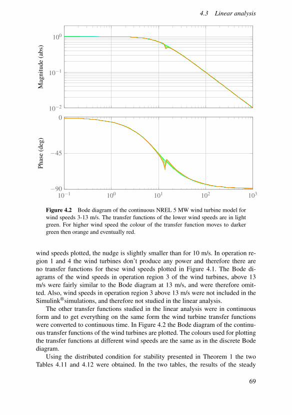
4.3 Linear analysis
10−2
10−1
100M
agni
tude
(abs
)
10−1 100 101 102 103−90
−45
0
Phas
e(d
eg)
Figure 4.2 Bode diagram of the continuous NREL 5 MW wind turbine model forwind speeds 3-13 m/s. The transfer functions of the lower wind speeds are in lightgreen. For higher wind speed the colour of the transfer function moves to darkergreen then orange and eventually red.
wind speeds plotted, the nudge is slightly smaller than for 10 m/s. In operation re-gion 1 and 4 the wind turbines don’t produce any power and therefore there areno transfer functions for these wind speeds plotted in Figure 4.1. The Bode di-agrams of the wind speeds in operation region 3 of the wind turbines, above 13m/s were fairly similar to the Bode diagram at 13 m/s, and were therefore omit-ted. Also, wind speeds in operation region 3 above 13 m/s were not included in theSimulink®simulations, and therefore not studied in the linear analysis.
The other transfer functions studied in the linear analysis were in continuousform and to get everything on the same form the wind turbine transfer functionswere converted to continuous time. In Figure 4.2 the Bode diagram of the continu-ous transfer functions of the wind turbines are plotted. The colours used for plottingthe transfer functions at different wind speeds are the same as in the discrete Bodediagram.
Using the distributed condition for stability presented in Theorem 1 the twoTables 4.11 and 4.12 were obtained. In the two tables, the results of the steady
69

Chapter 4. Results
state before any loss of generation and after the different cases of loss of generationare summarised. A slot is only labelled "Stable" if it satisfied Theorem 1 both forthe system before and after the loss of generations. For today’s case the loss ofgenerations were Oskarshamn 3 and Gigantic Gerhard. For the future scenario theloss of generation was the loss of a 290 turbine wind park, a 640 turbine windpark and Gigantic Gerhard. The linearisations were done in all of these situationsand the interconnected two node system was checked against Theorem 1. Since themodels used were all linear the main difference between before and after a faultwere the inertias and the amount of still on-line generators that was contributing tofrequency control. Since Theorem 1 only gives a sufficient condition for stability,the interconnected system can still be stable despite not satisfying Theorem 1. Justas mentioned in section 3.3 the feedback matrix K in Theorem 1 is Pmax
transmit
[1 −1−1 1
]with largest eigenvalue 2 ·Pmax
transmit .When checking Theorem 1 for the future system the Nyquist curves of PN and
PS both encircled the point −1/(2 ·Pmaxtransmit) for the cases; wind speed 6 m/s, 0%
of the wind turbines contributing to frequency control and after the loss of 290wind turbines, 640 wind turbines and Gigantic Gerhard. This also happened for awind speed of 7 m/s and 25% of the wind turbines contribution to frequency con-trol after the loss of 640 wind turbines and Gigantic Gerhard. However, if insteadlooking at −1/(2 ·Pmax
transmit cos(φnorth,0− φsouth,0)) both PN and PS did not encirclethis point. −1/(2 ·Pmax
transmit cos(φnorth,0−φsouth,0)) is the actual linearised transmis-sion feedback of the phase difference in the interconnected system. By looking atthe Nyquist curves in relation to −1/(2 ·Pmax
transmit) the worst case is examined. IfTheorem 1 is satisfied for −1/(2 ·Pmax
transmit) it is satisfied for all the different lev-els of transmission, this means that the linearised system is guaranteed to be stablealso for the dynamic behaviour right after the loss of generation. However, the sim-ulations of the future scenarios, of the wind speeds and amounts of wind turbinecontributing to frequency control in question, shows that the system is not unstablefor these situations.
70

4.3 Linear analysis
Table 4.11 The results of the linear analysis in today’s situation for Pmaxtransmit
Wind Amount of control of the wind turbines WindSpeed 0% 25% 50% 75% 100% Power2m/s Can’t tell Can’t tell Can’t tell Can’t tell Can’t tell 0.0%3m/s Can’t tell Can’t tell Can’t tell Can’t tell Can’t tell 0.2%4m/s Can’t tell Can’t tell Can’t tell Can’t tell Can’t tell 1.0%5m/s Can’t tell Can’t tell Can’t tell Can’t tell Can’t tell 3.1%6m/s Can’t tell Can’t tell Can’t tell Can’t tell Can’t tell 6.7%7m/s Can’t tell Can’t tell Can’t tell Can’t tell Can’t tell 11.4%8m/s Can’t tell Can’t tell Can’t tell Can’t tell Can’t tell 17.2%9m/s Can’t tell Can’t tell Can’t tell Can’t tell Can’t tell 23.6%
10m/s Can’t tell Can’t tell Can’t tell Stable Stable 30.6%11m/s Stable Stable Stable Stable Stable 37.8%12m/s Stable Stable Stable Stable Stable 45.3%13m/s Stable Stable Stable Stable Stable 45.3%26m/s Can’t tell Can’t tell Can’t tell Can’t tell Can’t tell 0.0%
Table 4.12 The results of the linear analysis in the future scanrio for Pmaxtransmit
Wind Amount of control of the wind turbines WindSpeed 0% 25% 50% 75% 100% Power2m/s Can’t tell Can’t tell Can’t tell Can’t tell Can’t tell 0.0%3m/s Can’t tell Can’t tell Can’t tell Can’t tell Can’t tell 0.8%4m/s Can’t tell Can’t tell Can’t tell Can’t tell Can’t tell 4.1%5m/s Can’t tell Can’t tell Can’t tell Can’t tell Can’t tell 13.1%6m/s Can’t tell Can’t tell Can’t tell Can’t tell Can’t tell 28.0%7m/s Can’t tell Can’t tell Can’t tell Can’t tell Can’t tell 48.0%8m/s Can’t tell Can’t tell Can’t tell Can’t tell Can’t tell 72.1%9m/s Can’t tell Can’t tell Stable Stable Stable 94.8%
10m/s Can’t tell Can’t tell Stable Stable Stable 94.8%11m/s Can’t tell Can’t tell Stable Stable Stable 94.8%12m/s Can’t tell Can’t tell Stable Stable Stable 94.8%13m/s Can’t tell Can’t tell Stable Stable Stable 94.8%26m/s Can’t tell Can’t tell Can’t tell Can’t tell Can’t tell 0.0%
71

Chapter 4. Results
4.4 PSS®E results
In this section the the frequency response of the loss of generators will be presentedfor the 400 kV buses in the Nordic 32 model. These buses are the ones in blue inFigure 3.13. In Appendix 3 PSS®E, the frequency response of the buses at 130 kVand 220 kV are shown. The voltages of all the buses and the active and reactivepower generated form all the generators can also be found in Appendix 3 PSS®E.
The frequency responses for all the 400 kV buses are plotted in the same graphfor a given scenario. This is because it would be redundant to plot the frequencyof each bus separately since they all generally follow the same pattern. To givean understanding of the geographical differences, the buses have different coloursin the figure depending on where they are in the system. The external buses areplotted in green. The other buses are plotted in a scale from blue to red. The bluestare the northernmost buses and the reddest are the southernmost. From north tosouth in Figure 3.13 (the one line diagram drawn in PSS®E), the buses are assignedcolours on a sliding scale from blue to red. Since the Nordic 32 model is not anexact representation of the Swedish or Nordic power grid one must remember thatFigure 3.13 is not an exact representation. However, the overall distribution of theregions given in Figure 3.11 and 3.12 are in line with the distribution in 3.13, so thecolour scaling can still give some insight to the behaviour in the north and south.The southern buses were drawn last in the plots and thus they are on top of the morenorthern buses. In the buses in the middle the roughly equal mix of red and blue inthe colour of the graphs gives a more purple colour.
0 5 10 15 20 25 30 35 40 45 50−0.15
−0.1
−0.05
0
0.05
0.1
Time s
Freq
uenc
yde
viat
ion
Hz
Figure 4.3 Frequency response of the 400 kV buses in today’s scenario, with theloss of generator g16 at time one second.
72

4.4 PSS®E results
0 5 10 15 20 25 30 35 40 45 50−0.15
−0.1
−0.05
0
0.05
0.1
Time s
Freq
uenc
yde
viat
ion
Hz
Figure 4.4 Frequency response of the 400 kV buses in the future scenario withoutfrequency control from the wind power generators, with the loss of generator g16 attime one second. The spikes in the plots are not predicted frequency at these time in-stances, but rather indications that PSS®E had problems performing the simulation.
In all the future simulations there are some spikes in the frequency responses,and also in the voltage and power responses at some time instances. These outliersin the output from the simulations were accompanied by messages about the "sim-ulation not converging" at these time instances. The spikes are rather an indicationof that PSS®E had problems performing the simulations, than that these spikes aresomething to expect in the real electric power system.
In Figure 4.3 the frequency response in the today’s case can be seen with theloss of generator g16, which was identified to correspond to Oskarshamn 3. In thissimulation the Nordic 32 model would not be able to cope with the loss of generatorg16, which can be seen as a rise in oscillations from about 5 seconds after the fault.Right after the loss of g16 the frequency went up in all the buses. This is not ex-plained by the simple first order transfer function model between power differenceand frequency deviation in equation (2.11). This is likely due to the instant voltageloss that can be seen in Figure 10.3 in Appendix 3. The voltage in the buses dropsimmediately after the loss of generator g16 and then quickly recovers some of thevoltage to be around a new lower average than before the fault. The voltage dropis the strongest in buses close to generator g16. Right after the loss of generatorg16 the reactive power of the generators still on-line rises quickly. After the initialsmall increase in frequency the average frequency follows the expected curve witha frequency nadir and a recovery. However, oscillations start to grow quickly andthe system seems to become unstable with larger oscillation as time passes.
73

Chapter 4. Results
0 5 10 15 20 25 30 35 40 45 50−0.15
−0.1
−0.05
0
0.05
0.1
Time s
Fequ
ency
devi
atio
nH
z
Figure 4.5 Frequency response of the 400 kV buses in the future scenario withfrequency control from the wind power generators, with the loss of generator g16 attime one second. The spikes in the plots are not predicted frequency at these time in-stances, but rather indications that PSS®E had problems performing the simulation.
0 5 10 15 20 25 30 35 40 45 50−0.3
−0.25
−0.2
−0.15
−0.1
−0.05
0
Time s
Freq
uenc
yde
viat
ion
Hz
Figure 4.6 Frequency response of the 400 kV buses in today’s scenario, with theloss of generator g9A at time one second.
74

4.4 PSS®E results
0 5 10 15 20 25 30 35 40 45 50−0.3
−0.25
−0.2
−0.15
−0.1
−0.05
0
Time s
Freq
uenc
yde
viat
ion
Hz
Figure 4.7 Frequency response of the 400 kV buses in the future scenario withoutfrequency control from the wind power generators, with the loss of generator g9A attime one second. The spikes in the plots are not predicted frequency at these time in-stances, but rather indications that PSS®E had problems performing the simulation.
0 5 10 15 20 25 30 35 40 45 50−0.3
−0.25
−0.2
−0.15
−0.1
−0.05
0
Time s
Freq
uenc
yde
viat
ion
Hz
Figure 4.8 Frequency response of the 400 kV buses in the future scenario withfrequency control from the wind power generators, with the loss of generator g9A attime one second. The spikes in the plots are not predicted frequency at these time in-stances, but rather indications that PSS®E had problems performing the simulation.
75

Chapter 4. Results
The frequency response of the future scenario in PSS®E without any frequencycontrol from the wind power generators, with the loss of g16 at time 1 second,can be seen in Figure 4.4. Also here the frequency initially goes up. However, itthen stays above the nominal frequency. The equation (2.11) cannot explain thisbehaviour. However, the voltage drops more significantly according to Figure 10.8and there is a significant increase in reactive power from the generators. Just like inthe present scenario, at the loss of generator g16, there are oscillation with growingamplitudes that eventually will make the system unstable.
If instead the controller with Kp = 4.0 and Ki = 0.2 was applied the frequencyresponse of the loss of generator g16 was slightly different. The frequency deviationof the 400 kV buses can be seen over the 50 second simulation time in Figure4.5. This response is slightly better, but still not good enough. It seems like thesystem would still become unstable with growing amplitudes of the oscillations offrequency deviation.
In Figure 4.6 the frequency in the present scenario can be seen with the loss ofgenerator g9A. This frequency behaviour looks much more like the the responsesin Figure 2.1. The response is very different from the present response at the lossof g16. To begin with, the loss of g9A is much smaller than the loss of g16, andthe generator g9A is connected to the rest of g9 that can contribute to the frequencycontrol.
The frequency deviation in the future scenario with the loss of g9A, withoutany frequency control from the wind power generators, is shown in Figure 4.7. Itlooks similar in shape to the present scenario, but with a lower frequency nadir andoscillations that starts to grow over time. The system would clearly not be stable forthis case since there is no sign of the oscillations dying out, rather the opposite.
If the wind turbines in the future scenario are contributing to frequency controlthe loss of generator g9A in the PSS®E model has the frequency deviation afterthe fault according to Figure 4.8 in the 400 kV buses. This frequency behaviourlooks much better than the behaviour without frequency control from the wind tur-bines. It is still not a perfect result since there are oscillations that don’t seem to bedecreasing in amplitude at the end of the simulation time.
76

5Discussion
Both the one node and two node Matlab®simulations indicates that if the nuclearpower stations would be decommissioned, and more wind turbines would be builtwithout contributing to the frequency control, the Swedish power system will pre-form worse in the future and possibly not be able to cope with a loss of generator ofa size that it can today. On the other hand, if wind turbines are contributing to fre-quency control in the future, the simulations indicate that the system can cope withthe same amount of loss of generation with similar performance, or even better. Theimprovement in performance, for a larger amount of wind turbines contributing tofrequency control, is the most at times with a lot of wind power.
From these results a reasonable strategy could be to let wind turbines operatelike they do today at low amounts of wind power in the system, and at high amountsof wind power they could be used for frequency control by curtailing some wind.From an economic perspective this would also make sense. If there are a lot of windturbines in the future the price of electricity would be very low during days with alot of wind because many wind turbine operators could produce the electricity. Inthis case the companies that owns wind power could curtail some of the wind andinstead sell the the service of contributing to frequency containment reserve. Todaymostly hydro power contributes to the frequency containment reserve. If the hydropower plants don’t have to contribute to the frequency containment reserve theycan save water in their reservoirs for days when they get better paid for the power.Since wind turbines can’t save the energy it would therefore be more economicallyreasonable to use as little hydro power as possible and instead use wind turbines forthe frequency containment reserve. During days with little wind power there wouldinstead be a lot of hydro power active and these could then, just like today, make upmost of the frequency containment reserve.
Storage was not included in this thesis, but in a future with a lot of wind turbinesthe price of electricity will likely be low on windy days and high on less windy days.Therefore, there could definitely be a market for this in the a future with a lot of windpower. Storage of power can be done in several different ways. For example it canbe done with batteries, fuel cells and pumped hydro. There is a lot of active hydropower in the Nordic system today. As was seen in the future scenario simulations in
77

Chapter 5. Discussion
Matlab®, wind power can at windy days produce more power than consumed, if it isincreased by 320%, to replace the nuclear generation. In a case like that, just to notuse hydro power is not enough to store energy. With pumped hydro, water can bepumped from a lower reservoir to a higher one when electric power is abundant, andthen let the water run down, powering a generator when electric power is needed.Hydrogen could also be used for storage of power. At times with a lot of availableelectric power hydrogen can be produced and stored. Then, at times of low poweravailability fuel cells can be used to turn the hydrogen, and oxygen in the air, toelectric power and water.
In this thesis the effects of using wind turbines for frequency control have beenstudied. It was concluded that the performance would worsen in the future if windturbines don’t contribute to frequency control and the inertia is reduced. However,an alternative way to counter this would be to add inertia in another way. This canfor example be done by using flywheels. By using a flywheel energy can be stored inthe same way as in a rotating generator, i.e. as kinetic energy of rotating masses, byhaving it electromagnetically coupled to the grid. If the frequency of the grid woulddecrease the flywheel would slow down, thus converting some of the mechanicalenergy to electric power. This is often called a synchronous compensator. However,when a flywheel is rotating, energy is lost both in friction and through the Coriolisforce, from the rotation of earth. A way to minimize these effects is to use magneticbearings for holding the flywheel, let it rotate in vacuum to limit the air resistanceand to let it rotate in line with the earth’s axle of rotation [Amyriar and Pullen,2017].
In the Matlab®simulation only Sweden was modelled even though Sweden istightly connected to the Nordic synchronous system. In a more accurate model thiswould have been taken into account. The reason only Sweden was modelled wasbecause of the easy access to historic data in Sweden. Further, a two node modelcan be seen as rather representative for the Swedish power system, because of thegeographical shape of Sweden. For a full Nordic model a two node approximationwould not be as representative.
Further, when building the Matlab®model of the Swedish power grid electricityarea 1 and 2 were added together in the northern node and electricity area 3 and 4were added together in the southern. Since the data exists for all these four nodes afour node model could have been built just like the two node model.
In the two node simulations the same wind speed was used in both the nodes.This was done to limit the amount of simulations. A better coverage of the differ-ent situations could have been obtained if the wind speeds were different in thetwo nodes. However, the objective of the Matlab®simulations was to investigate thetendencies of the behaviour, depending on different amounts of the wind turbinescontributing to frequency control, under different amounts of wind power in thesystem. This could still be done with the same wind speed in both nodes. If one isinterested in knowing the dynamics more accurately, and the actual consequencesof more wind turbines in the Swedish power system a more detailed model than the
78

Chapter 5. Discussion
ones used in the Matlab®simulations is needed.In the future scenario in the Matlab®simulations it was assumed the load-
frequency dependency will be the same in the future as today. With more and moreelectric devices using an inverter between the grid and the device, like convertercontrolled induction machines, this might not be the case in the future.
The linear analysis tool used in this report is a rather blunt tool. It can only sayif something is guaranteed to be stable. The simulations shows that there are maycases when the performance of the system was rather good, but the linear analysiscouldn’t say that it was stable. Further, to say that a system is stable is not the sameas to say that it performs good. For example, if there would be a power imbalancein the Matlab®model between consumed and produced electric power, without anyfrequency control from any of the generating sources, the frequency would end upat a new frequency according to equation (2.12). This is if the linear model couldstill be considered to be valid. This situation would be considered stable from acontrol sense, even though the frequency could deviate a lot from the nominal, andthe linearisation might not be valid any more. At the same time, the distributedcondition for stability only investigates if the combined system could fall outsidethe necessary conditions for stability at the maximum feedback transfer of power.The system might very well fulfil the distributed conditions for stability at the actualtransmission.
When performing the linear analysis it was discovered that the main obstacleagainst satisfying Theorem 1 was in the transfer function of the northern node. It issuspected that the non-minimum phase dynamics in the hydro power is the reasonfor this. In the linear analysis the model for hydro power was the same as in thesimulation. This model was obtained from Svenska kraftnät in [Robert Eriksson,2017] and [Robert Eriksson, 2017]. In this modelling of the hydro it is assumed thatall hydro power stations act to control the frequency. If instead a smaller amountof the hydro power actually contributes to the frequency control the non-minimumphase dynamics would not be that significant and thus more situations might sat-isfy the distributed condition of Theorem 1. In the two node simulation the actualpower transmitted is known since the model is very simple. The great advantagewith the distributed condition is that it can be applied when the exact power trans-mitted isn’t known. From the discussion in section 3.3 it is known that the steadysate power flow solution is not trivial for more detailed power grid. By looking atthe maximum powers that can be transmitted in a system a check can be done tosee if stability is guaranteed. Buses in the system that don’t fulfil the distributedcondition of Theorem 1 can then be further investigated. A great advantage of usingthe distributed condition is when connecting a new bus, for example a new windturbine. It can then be guaranteed that this new bus does not risk any of the stabilityin the already existing system and a controller at that wind turbine can be designedso that the bus satisfies Theorem 1. The way the distributed condition of Theorem1 was used in this thesis is not where is has the most potential. Here it was used ontwo large nodes with lumped together generating sources.
79

Chapter 5. Discussion
What the distributed condition in Theorem 1 basically tests for all nodes (whichby themselves are stable) is if the power transmission to and from that node has theability to disturbed the node more that the node can stabilise. If all nodes are stablewithout any transmission and the transmissions to and from all nodes are not enoughto disturb the nodes more than they can handle, then the total system is guaranteedto be stable.
In the unchanged model in PSS®E model from [Thierry Van Cutsem, 2015]there are stabilisers put in place on all generators. The stabilisers used are IEEESTand these help stabilise the voltage in the system. When implementing the windpower generators there was no possibility to give them stabilisers. Therefore, whenconverting generators g15, g16 and g18 to wind generators the stabilisers associ-ated with these generators were effectively removed. This can be a reason for theoscillation that occur in all the PSS®E simulation with wind power generators.
The wind generator models already existing in PSS®E are not developed tosupport frequency control, since wind turbines are not conventionally used for fre-quency control. Therefore, using them for frequency control as has been done in thisthesis is not unproblematic. This can be a reason why the PSS®E simulations withwind turbines behaved so unexpectedly, in particular in the future scenario with theloss of generator g16 and no frequency control from the wind generators.
In the plots for active power in the future scenario, there is not much differ-ence between the active power generated from wind generators, with or withoutfrequency control from wind power. This was very unexpected and does not at allresemble what was found in the Matlab®simulations. On the other hand, the windgeneration does differ in reactive power output for the case with and without control.Further, especially for the loss of generator g9A, there was a major improvementin the frequency response after the loss of generator g9A when the wind generatorscontributed to frequency control, compared to when they didn’t (see Figure 4.7 and4.8). Further investigation into this is thus needed to conclude how wind turbinescan improve the performance of a system if they contribute with frequency control.
In Figure 4.3 the present case frequency response of the loss of generator g16 isshown. Already the present case simulation could not cope with the loss of generatorg16, so trying to simulate what would happen in a case with much less inertia in thesystem might not have been the best approach. Rather an approach similar to theone taken for the generator g9A could have been good, i.e. splitting the generator intwo and simulate the loss of just one of these.
80

6Conclusion
Even though the results are not showing exactly the same thing they are all indicat-ing in the same direction. With more power in a power system coming from windpower the inertia goes down and the system preforms worse than today. With fre-quency control from wind turbines this worsened behaviour can be improved, andit is worth looking into this for a future with more wind power in the total mix.The Simulink®simulations and the distributed condition show that the future sys-tem has the ability to actually perform better than today’s system if wind turbinesare used for frequency control, despite the reduced inertia. This is because hydropower generators are inherently limited to act fast because of the non-minimumphase dynamics of water flow. Wind turbines don’t have this disadvantage and canthus act much faster. The PSS®E simulations also showed improvident when usingwind turbines for frequency control, although not as conclusive.
81

7Future work
This thesis only looked at the effects of lower inertia in the system from non-synchronous machines in the electric power grid, and if frequency control fromwind turbines could overcome the difficulties. Another aspect to look into is the ef-fect of reduced load-frequency dependency in a future system. This was chosen notto be done in this thesis.
The simulations done in Matlab®and the Simulink®models were very simpli-fied. To get a more detailed understanding of the future scenario presented a moredetailed model would be needed. In the PSS®E simulations a pre-defined modelof a wind generator was used. This model has not been developed to be used forfrequency control. Therefore, to develop a wind generator model and use this insimilar simulation as was done in this thesis could be of interest.
In all parts of the process only PI controllers with droop control were consid-ered. The reason for this was that wind generator model in PSS®E only had PIcontroller as an option. A study of other types of controllers could give better re-sults. However, this should be accompanied by more detailed models to get a moreaccurate simulation result. Once a well performing control strategy for a more ac-curate model has been obtained a future task can also be to express it in terms ofthe way frequency control is organized today i.e. in terms of FFR, FCR-N, FCR-D,aFRR and mFRR.
In the Matlab®simulations only a 10% curtailment of output power was investi-gated. Further work could be done by investigating other possible curtailments, andsee if this affects the performance. Another interesting topic would be to look intoif the frequency stability is affected by gusts in the wind.
The distributed conditions were only applied to the linear models. A more de-tailed understanding could be to instead look at a non-linear model and investigateregions of attractions, e.g. the systems ability to recover power difference and getthe frequency back to a tolerable region after a major loss of generation.
82

Bibliography
“Advanced Power System Analysis - An Introduction to PSS®E” (2019). ChalmersUniversity of Technology.
Amyriar, M. E. and K. R. Pullen (2017). “A review of flywheel energy storagesystem technologies and their applications”. MDPI.
Elorza, I., C. Calleja, and A. Pujana-Arrese (2019). “On wind turbine power deltacontrol”. MDPI.
Elstatistik - Statistik hela landet per månad 2019(xls). Accessed: 2020-06-11. URL:https://www.svk.se/aktorsportalen/elmarknad/kraftsystemdata/elstatistik/.
Elstatistik - Statistik per elområde och timme, 2019(xls). Accessed: 2020-07-15. URL: https : / / www . svk . se / aktorsportalen / elmarknad /kraftsystemdata/elstatistik/.
Energiföretagen - Kraftvärme. Accessed: 2020-07-28. URL: https : / / www .energiforetagen.se/energifakta/kraftvarme/.
Energy Systems Integration Group - WT4 Generic Wind Model. Accessed: 2020-06-10. URL: https://www.esig.energy/wiki-main-page/wt4-generic-wind-model/#Generator.2FConverter_Model_.28WT4G.29.
ENERGY USE IN SWEDEN. Accessed: 2020-01-24. URL: \url{https : / /sweden.se/nature/energy-use-in-sweden/}.
entso-e - System Operations Committee. Accessed: 2020-08-02. URL: https://www.entsoe.eu/about/system-operations/.
Hägglund, T. (2019). REGLERTEKNIK AK Föreläsningar. Institutionen för Re-glerteknik, Lunds Tekniska Högskola.
Info on Svensk vattenkraft - Övrsikt Sverige. Accessed: 2020-07-26. URL: https://vattenkraft.info/?page=5.
J. Driesen, K. (2008). “Virtual synchronous generators”. IEEE.J. Duncan Glover Mulukutla S. Sarma, T. J. O. (2010). Power System Analysis and
Design. Cengage Learning.
83

Bibliography
J.F Manwell, J. M. A. R. (2009). Wind Energy Explained. Wiley.Jonkman, J., S. Butterfield, W. Musial, and G. Scott (2009). “Definition of a 5-
mw reference wind turbine for offshore system development”. Technical ReportNREL/TP-500-38060.
Kundur, P. (1994). Power System Stability and Control. R.R. Donnelley and SonsCompany.
Mallada, E. (2016). “Idroop: a dynamic droop controller to decouple power grid’ssteady-state and dynamic performance”. IEEE 55th Conference on Decision andControl (CDC).
Masson-Delmotte, V., P. Zhai, H.-O. Pörtner, D. Roberts, J. Skea, P. Shukla, W A.Pirani, Moufouma-Okia, C. Péan, R. Pidcock, S. Connors, J. Matthews, Y. Chen,X. Zhou, M. Gomis, E. Lonnoy, T. Maycock, M. Tignor, and T. W. (eds.) (2018).Global Warming of 1.5°C. An IPCC Special Report on the impacts of globalwarming of 1.5°C above pre-industrial levels and related global greenhousegas emission pathways, in the context of strengthening the global response tothe threat of climate change, sustainable development. IPCC.
Mikko Kuivaniemi Niklas Modig, R. E. (2017). “Fcr-d design of requirements”.entso-e.
“NETWORK DEVELOPMENT PLAN 2016 – 2025” (2015). Svenska kraftnät.Nord Pool - Transmission capacity prognosis. Accessed: 2020-07-28. URL: https:
//www.nordpoolgroup.com/Market-data1/Dayahead/Capacities1/new- transmission- capacity- prognosis/SE/daily- week- ahead/?view=table.
okg - Oskarshamn 3. Accessed: 2020-07-25. URL: https://www.okg.se/sv/Karnkraft/Anlaggningar/Oskarshamn-3/.
Operational Constraints Update 29/03/2019. Accessed: 2020-01-24, EirGrid plc,the Transmission System Operator (TSO) for Ireland, and SONI Limited, theTSO for Northern Ireland. URL: \url{http://www.eirgridgroup.com/site-files/library/EirGrid/Operational-Constraints-Update-Mar_2019.pdf}.
R. Pates, E. M. (2019). Robust Scale-Free Synthesis for Frequency Control in PowerSystems. arXiv:1804.00729 [math.OC].
Robert Eriksson Niklas Modig, A. W. (2017). “Fcr-n design of requirements”.entso-e.
Siemens Power Technologies International - PSS®E 34.2.0 MODEL LIBRARY(2017).
Siemens PSS®E – high-performance transmission planning and analysis software.Accessed: 2020-06-05. URL: https://new.siemens.com/global/en/products/energy/services/transmission- distribution- smart-grid/consulting-and-planning/pss-software/pss-e.html.
84
Bibliography
SimWindFarm - Simplified NREL5MW turbine for Simulink. Accessed: 2020-03-05.URL: \url{ict-aeolus.eu/SimWindFarm/index.html}.
Storuman enegi AB - Om jämförpriser. Accessed: 2020-08-15. URL: https://www.storumanenergi.se/om-jamforpriser/.
Strålsäkerhatsmyndigheten - Kärnkraft. Accessed: 2020-07-23. URL: https://www.stralsakerhetsmyndigheten.se/omraden/karnkraft/.
Stubbe, M (1995). “Long term dynamics phase ii - final report”. CIGRE Task Force38.02.08.
Svensk Vindenergi – Swedish Wind Energy Association, SWEA: Statistics and fore-cast. Accessed: 2020-07-15. URL: https://svenskvindenergi.org/wp-content / uploads / 2020 / 02 / Statistics - and - forecast - Svensk -Vindenergi-feb-2020-FINAL.pdf.
Svenska Kraftnät - Information om stödtjänster. Accessed: 2020-08-19. URL:https://www.svk.se/aktorsportalen/elmarknad/information-om-stodtjanster/.
Svenska Kraftnät - Map of the national grid. Accessed: 2020-07-28. URL: https://www.svk.se/siteassets/drift-av-stamnatet/bilder/map-of-the-national-grid.pdf.
Svenska kraftnät - Störningsreserven. Accessed: 2020-07-24. URL: https://www.svk.se/aktorsportalen/elmarknad/information-om-stodtjanster/storningsreserven/.
Svenska Kraftnät - The control room. Accessed: 2020-08-02. URL: https://www.svk.se/en/national-grid/the-control-room/.
Svenska Kraftnät - Översiktlig kravbild för reserver. Accessed: 2020-08-19. URL:https : / / www . svk . se / siteassets / aktorsportalen / elmarknad /information-om-reserver/reservmarknader.pdf.
Thierry Van Cutsem Mevludin Glavic, W. R. (2015). “Test systems for voltage sta-bility analysis and security assessment”. IEEE Power & Energy Society Techni-cal report PES-TR19.
Vattenfall - Harsprånget. Accessed: 2020-07-25. URL: https://powerplants.vattenfall.com/harspranget.
World Nuclear Association - Nuclear Power in Sweden. Accessed: 2020-07-28.URL: https : / / www . world - nuclear . org / information - library /country-profiles/countries-o-s/sweden.aspx.
Ørum, E., M. Kuivaniemi, Minna, Laasonen, A. I. Bruseth, E. A. Jansson, A.Danell, K. Elkington, and N. Modig (2015). “Nordic report future system in-ertia”. entso-e.
85

8Appendix 1 Plots of some ofthe Simulink®simulations
In this appendix plots of the frequency and power from the different types of gen-eration are shown. The generation labelled "Thermal" is nuclear power and otherthermal. The situations plotted are the two node simumulations with backlash inthe hydro power at a wind speed of 7 m/s with 0%, 50% and 100% of the windturbines contributing to frequency control. 7 m/s was chosen because it is close tothe average wind speed in the present system, and is in the middle of the differentwind speed investigated in the Simulink®simulations. In the figures the uppermostplot is for 0% of the wind turbines contributing to frequency control, the middle iswhen 50% of the wind turbines contributing, and the bottommost is when all windturbines contribute to frequency control. The situations plotted are the following.
• The loss of Oskarshamn 3 at time 0 in today’s system (Figure 8.1)
• The loss of Gigantic Gerhard at time 0 in today’s system (Figure 8.2)
• The loss of 290 5 MW wind turbines at time 0 in the future scenario system(Figure 8.3)
• The loss of 640 5 MW wind turbines at time 0 in the future scenario system(Figure 8.4)
• The loss of Gigantic Gerhard at time 0 in future scenario system (Figure 8.5)
86

Chapter 8. Appendix 1 Plots of some of the Simulink®simulations
−1.5
−1
−0.5
0Fr
eque
ncy
devi
atio
nH
z
NorthSouth
0 5 10 15 20 25 30 35 40 45 500
0.4
0.8
1.2·104
Pow
erM
W
ThermalHydroWind
−1.5
−1
−0.5
0
Freq
uenc
yde
viat
ion
Hz
NorthSouth
0 5 10 15 20 25 30 35 40 45 500
0.4
0.8
1.2·104
Pow
erM
W
ThermalHydroWind
−1.5
−1
−0.5
0
Freq
uenc
yde
viat
ion
Hz
NorthSouth
0 5 10 15 20 25 30 35 40 45 500
0.4
0.8
1.2·104
Time s
Pow
erM
W
ThermalHydroWind
Figure 8.1 Simulation result with the loss of Oskarshamn 3 at time 0 in today’ssystem. The plots are order of amount of wind turbines doing frequency control(0%, 50% and 100%). 87

Chapter 8. Appendix 1 Plots of some of the Simulink®simulations
−1.5
−1
−0.5
0Fr
eque
ncy
devi
atio
nH
z
NorthSouth
0 5 10 15 20 25 30 35 40 45 500
0.4
0.8
1.2·104
Pow
erM
W
ThermalHydroWind
−1.5
−1
−0.5
0
Freq
uenc
yde
viat
ion
Hz
NorthSouth
0 5 10 15 20 25 30 35 40 45 500
0.4
0.8
1.2·104
Pow
erM
W
ThermalHydroWind
−1.5
−1
−0.5
0
Freq
uenc
yde
viat
ion
Hz
NorthSouth
0 5 10 15 20 25 30 35 40 45 500
0.4
0.8
1.2·104
Time s
Pow
erM
W
ThermalHydroWind
Figure 8.2 Simulation result with the loss of Gigantic Gerhard at time 0 in today’ssystem. The plots are order of amount of wind turbines doing frequency control (0%,50% and 100%).88

Chapter 8. Appendix 1 Plots of some of the Simulink®simulations
−1.5
−1
−0.5
0Fr
eque
ncy
devi
atio
nH
z
NorthSouth
0 5 10 15 20 25 30 35 40 45 500
0.4
0.8
1.2·104
Pow
erM
W
ThermalHydroWind
−1.5
−1
−0.5
0
Freq
uenc
yde
viat
ion
Hz
NorthSouth
0 5 10 15 20 25 30 35 40 45 500
0.4
0.8
1.2·104
Pow
erM
W
ThermalHydroWind
−1.5
−1
−0.5
0
Freq
uenc
yde
viat
ion
Hz
NorthSouth
0 5 10 15 20 25 30 35 40 45 500
0.4
0.8
1.2·104
Time s
Pow
erM
W
ThermalHydroWind
Figure 8.3 Simulation result with the loss of 290 wind turbines at time 0 in the fu-ture scenario system. The plots are order of amount of wind turbines doing frequencycontrol (0%, 50% and 100%). 89

Chapter 8. Appendix 1 Plots of some of the Simulink®simulations
−1.5
−1
−0.5
0Fr
eque
ncy
devi
atio
nH
z
NorthSouth
0 5 10 15 20 25 30 35 40 45 500
0.4
0.8
1.2·104
Pow
erM
W
ThermalHydroWind
−1.5
−1
−0.5
0
Freq
uenc
yde
viat
ion
Hz
NorthSouth
0 5 10 15 20 25 30 35 40 45 500
0.4
0.8
1.2·104
Pow
erM
W
ThermalHydroWind
−1.5
−1
−0.5
0
Freq
uenc
yde
viat
ion
Hz
NorthSouth
0 5 10 15 20 25 30 35 40 45 500
0.4
0.8
1.2·104
Time s
Pow
erM
W
ThermalHydroWind
Figure 8.4 Simulation result with the loss of 640 wind turbines at time 0 in the fu-ture scenario system. The plots are order of amount of wind turbines doing frequencycontrol (0%, 50% and 100%).90

Chapter 8. Appendix 1 Plots of some of the Simulink®simulations
−1.5
−1
−0.5
0Fr
eque
ncy
devi
atio
nH
z
NorthSouth
0 5 10 15 20 25 30 35 40 45 500
0.4
0.8
1.2·104
Pow
erM
W
ThermalHydroWind
−1.5
−1
−0.5
0
Freq
uenc
yde
viat
ion
Hz
NorthSouth
0 5 10 15 20 25 30 35 40 45 500
0.4
0.8
1.2·104
Pow
erM
W
ThermalHydroWind
−1.5
−1
−0.5
0
Freq
uenc
yde
viat
ion
Hz
NorthSouth
0 5 10 15 20 25 30 35 40 45 500
0.4
0.8
1.2·104
Time s
Pow
erM
W
ThermalHydroWind
Figure 8.5 Simulation result with the loss of Gigantic Gerhard at time 0 in the fu-ture scenario system. The plots are order of amount of wind turbines doing frequencycontrol (0%, 50% and 100%). 91

9Appendix 2Matlab®simulations with nobacklash
In section 4.1 and 4.2 the simulation results of the one node and two nodeMatlab®simulations were presented. In the Simulink®model used there was back-lash in the hydro power model. In the linear analysis non-linearities like backlashand saturations were omitted. In the following appendix the results of the one andtwo node Matlab®simulations without backlash in the hydro power model are pre-sented. The stimulations are the same that was done in the model with backlash.
The reason for including these results in the report is to show that the modelused in the simulations for the results in section 4.1 and 4.2 are very similar to theones used for the linear analysis, with respect to performance. The main differenceis that the recovery time is less sporadic than with backlash in the hydro power. Oneinteresting result that was found in the simulations with and without backlash is thatthe system without backlash in the hydro power is slightly more difficult to controlafter a major loss of generation. The reason for this is that the backlash slightlycompensates for the non-minimum phase dynamics.
9.1 One node model
In the following tables the result of the one node Matlab®simulation, without back-lash, are presented. The cases presented are the following:
• Present average scenario with the loss of Oskarshamn 3 (Table 9.1)
• Present average scenario with the loss of Gigantic Gerhard (Table 9.2)
• The future scenario described in section 3.1 with the loss of a wind park with290 turbines (Table 9.3)
92

9.1 One node model
Table 9.1 Table of the frequency nadir and recovery time in the present scenario,one node simulation, with the loss of Oskarshamn 3 for different wind speeds anddifferent amounts of the wind turbines contributing to frequency control. The inertiaof the system after the loss of power, and the percentage of the total power that isproduced by wind turbines, at that particular wind speed are also presented.
Wind Amount of control of the wind turbines Inertia WindSpeed 0% 25% 50% 75% 100% H Power
−1.59Hz −1.59Hz −1.59Hz −1.59Hz −1.59Hz2m/s
35.4s 35.4s 35.4s 35.4s 35.4s4.27s 0.0%
−1.59Hz −1.59Hz −1.59Hz −1.59Hz −1.59Hz3m/s
35.5s 35.2s 34.9s 34.5s 34.0s4.26s 0.2%
−1.59Hz −1.59Hz −1.59Hz −1.59Hz −1.58Hz4m/s
35.4s 35.3s 35.2s 35.2s 35.1s4.25s 1.0%
−1.61Hz −1.60Hz −1.59Hz −1.58Hz −1.58Hz5m/s
35.3s 35.2s 35.2s 35.2s 35.2s4.20s 3.1%
−1.62Hz −1.61Hz −1.59Hz −1.57Hz −1.56Hz6m/s
35.1s 35.2s 35.2s 35.2s 35.3s4.13s 6.7%
−1.64Hz −1.62Hz −1.59Hz −1.56Hz −1.53Hz7m/s
34.9s 35.1s 35.2s 35.4s 35.5s4.04s 11.4%
−1.67Hz −1.63Hz −1.59Hz −1.54Hz −1.50Hz8m/s
34.6s 35.0s 35.2s 35.5s 35.7s3.92s 17.2%
−1.71Hz −1.65Hz −1.59Hz −1.53Hz −1.47Hz9m/s
34.2s 34.8s 35.2s 35.6s 35.9s3.79s 23.6%
−1.75Hz −1.67Hz −1.59Hz −1.52Hz −1.44Hz10m/s
33.8s 34.6s 35.2s 35.8s 36.2s3.65s 30.6%
−1.79Hz −1.69Hz −1.60Hz −1.50Hz −1.41Hz11m/s
33.4s 34.4s 35.2s 35.9s 36.6s3.50s 37.8%
−1.84Hz −1.73Hz −1.61Hz −1.49Hz −1.38Hz12m/s
32.9s 34.2s 35.2s 36.1s 37.0s3.35s 45.3%
−1.84Hz −1.73Hz −1.61Hz −1.49Hz −1.38Hz13m/s
32.9s 34.2s 35.2s 36.1s 37.0s3.35s 45.3%
26m/s−1.59Hz −1.59Hz −1.59Hz −1.59Hz −1.59Hz
4.27s 0.0%35.5s 35.5s 35.5s 35.5s 35.5s
• The future scenario described in section 3.1 with the loss of a wind park with640 turbines (Table 9.4)
• The future scenario described in section 3.1 with the loss of Gigantic Gerhard(Table 9.5)
The comments about the results in chapter 5.1 are also valid for the results here.
93

Chapter 9. Appendix 2 Matlab®simulations with no backlash
Table 9.2 Table of the frequency nadir and recovery time in the present scenario,one node simulation, with the loss of Gigantic Gerhard for different wind speeds anddifferent amounts of the wind turbines contributing to frequency control. The inertiaof the system after the loss of power, and the percentage of the total power that isproduced by wind turbines, at that particular wind speed are also presented.
Wind Amount of control of the wind turbines Inertia WindSpeed 0% 25% 50% 75% 100% H Power
−0.47Hz −0.47Hz −0.47Hz −0.47Hz −0.47Hz2m/s
36.7s 36.7s 36.7s 36.7s 36.7s4.70s 0.0%
−0.47Hz −0.47Hz −0.47Hz −0.47Hz −0.47Hz3m/s
36.7s 36.3s 36.1s 35.9s 35.8s4.69s 0.2%
−0.47Hz −0.47Hz −0.47Hz −0.47Hz −0.47Hz4m/s
36.7s 36.3s 36.2s 36.0s 36.0s4.68s 1.0%
−0.48Hz −0.47Hz −0.46Hz −0.46Hz −0.45Hz5m/s
36.6s 36.4s 36.4s 36.3s 36.3s4.63s 3.1%
−0.48Hz −0.47Hz −0.45Hz −0.44Hz −0.42Hz6m/s
36.4s 36.6s 36.7s 36.9s 37.0s4.56s 6.7%
−0.49Hz −0.46Hz −0.43Hz −0.41Hz −0.38Hz7m/s
36.2s 36.8s 37.2s 37.6s 38.0s4.47s 11.4%
−0.49Hz −0.45Hz −0.42Hz −0.38Hz −0.35Hz8m/s
36.1s 37.0s 37.9s 38.9s 40.2s4.35s 17.2%
−0.50Hz −0.45Hz −0.40Hz −0.36Hz −0.32Hz9m/s
35.8s 37.4s 38.4s 38.9s 38.8s4.22s 23.6%
−0.51Hz −0.45Hz −0.40Hz −0.36Hz −0.33Hz10m/s
35.5s 36.7s 36.9s 37.4s 37.8s4.08s 30.6%
−0.52Hz −0.46Hz −0.41Hz −0.37Hz −0.33Hz11m/s
35.1s 35.9s 36.6s 37.1s 37.5s3.93s 37.8%
−0.53Hz −0.47Hz −0.41Hz −0.37Hz −0.34Hz12m/s
34.7s 35.5s 36.2s 36.7s 37.2s3.78s 45.3%
−0.53Hz −0.47Hz −0.41Hz −0.37Hz −0.34Hz13m/s
34.7s 35.5s 36.2s 36.7s 37.2s3.78s 45.3%
26m/s−0.47Hz −0.47Hz −0.47Hz −0.47Hz −0.47Hz
4.70s 0.0%36.7s 36.7s 36.7s 36.7s 36.7s
94

9.1 One node model
Table 9.3 Table of the frequency nadir and recovery time in the future scenario,one node simulation, with the loss of 290 wind turbines for different wind speedsand different amounts of the wind turbines contributing to frequency control. Theinertia of the system after the loss of power, and the percentage of the total powerthat is produced by wind turbines, at that particular wind speed are also presented.
Wind Amount of control of wind turbines Inertia WindSpeed 0% 25% 50% 75% 100% H Power
- - - - -2m/s
- - - - -3.13s 0.0%
−0.01Hz −0.01Hz −0.00Hz −0.00Hz −0.00Hz3m/s
32.0s 36.9s 39.8s 37.5s 38.2s3.10s 0.8%
−0.04Hz −0.03Hz −0.02Hz −0.01Hz −0.01Hz4m/s
31.4s 36.6s 39.6s 37.6s 37.9s2.94s 4.1%
−0.13Hz −0.10Hz −0.07Hz −0.04Hz −0.04Hz5m/s
30.8s 36.2s 39.3s 37.5s 37.4s2.76s 13.1%
−0.31Hz −0.23Hz −0.15Hz −0.10Hz −0.08Hz6m/s
29.8s 35.5s 38.7s 37.3s 36.7s2.46s 28.0%
−0.63Hz −0.46Hz −0.30Hz −0.19Hz −0.14Hz7m/s
41.2s 34.5s 37.9s 37.2s 35.5s2.06s 48.0%
−1.26Hz −0.91Hz −0.59Hz −0.35Hz −0.23Hz8m/s
in f s 34.4s 36.6s 37.0s 33.7s1.57s 72.1%
−2.27Hz −0.97Hz −0.55Hz −0.32Hz −0.25Hz9m/s
in f s in f s 37.3s 36.4s 37.8s1.12s 94.8%
−2.27Hz −0.97Hz −0.55Hz −0.32Hz −0.25Hz10m/s
in f s in f s 37.3s 36.4s 37.8s1.12s 94.8%
−2.27Hz −0.97Hz −0.55Hz −0.32Hz −0.25Hz11m/s
in f s in f s 37.3s 36.4s 37.8s1.12s 94.8%
−2.27Hz −0.97Hz −0.55Hz −0.31Hz −0.25Hz12m/s
in f s in f s 37.3s 36.4s 37.8s1.12s 94.8%
−2.27Hz −0.97Hz −0.55Hz −0.31Hz −0.25Hz13m/s
in f s in f s 37.3s 36.4s 37.8s1.12s 94.8%
- - - - -26m/s
- - - - -3.13s 0.0%
95

Chapter 9. Appendix 2 Matlab®simulations with no backlash
Table 9.4 Table of the frequency nadir and recovery time in the future scenario,one node simulation, with the loss of 640 wind turbines for different wind speedsand different amounts of the wind turbines contributing to frequency control. Theinertia of the system after the loss of power, and the percentage of the total powerthat is produced by wind turbines, at that particular wind speed are also presented.
Wind Amount of control of the wind turbines Inertia WindSpeed 0% 25% 50% 75% 100% H Power
- - - - -2m/s
- - - - -3.13s 0.0%
−0.02Hz −0.01Hz −0.01Hz −0.01Hz −0.01Hz3m/s
32.0s 34.7s 36.1s 37.2s 38.4s3.10s 0.8%
−0.09Hz −0.08Hz −0.07Hz −0.06Hz −0.05Hz4m/s
31.4s 34.4s 35.9s 37.1s 38.3s2.94s 4.1%
−0.30Hz −0.26Hz −0.22Hz −0.19Hz −0.15Hz5m/s
30.8s 34.0s 35.8s 37.0s 38.3s2.76s 13.1%
−0.69Hz −0.61Hz −0.53Hz −0.44Hz −0.36Hz6m/s
29.8s 33.3s 35.4s 36.9s 38.2s2.46s 28.0%
−1.40Hz −1.23Hz −1.06Hz −0.89Hz −0.73Hz7m/s
41.2s 32.4s 35.0s 36.7s 38.2s2.06s 48.0%
−2.77Hz −2.41Hz −2.08Hz −1.76Hz −1.44Hz8m/s
in f s 30.2s 34.4s 36.6s 38.4s1.57s 72.1%
−4.19Hz −2.83Hz −2.40Hz −1.98Hz −1.58Hz9m/s
in f s in f s 34.9s 37.0s 39.0s1.12s 94.8%
−4.19Hz −2.83Hz −2.40Hz −1.98Hz −1.58Hz10m/s
in f s in f s 34.9s 37.0s 39.0s1.12s 94.8%
−4.19Hz −2.83Hz −2.40Hz −1.98Hz −1.57Hz11m/s
in f s in f s 34.9s 37.0s 39.0s1.12s 94.8%
−4.18Hz −2.83Hz −2.40Hz −1.98Hz −1.57Hz12m/s
in f s in f s 34.9s 37.0s 39.0s1.12s 94.8%
−4.18Hz −2.83Hz −2.40Hz −1.98Hz −1.57Hz13m/s
in f s in f s 34.8s 37.0s 39.0s1.12s 94.8%
- - - - -26m/s
- - - - -3.13s 0.0%
96

9.1 One node model
Table 9.5 Table of the frequency nadir and recovery time in the future scenario,one node simulation, with the loss of Gigantic Gerhard for different wind speeds anddifferent amounts of the wind turbines contributing to frequency control. The inertiaof the system after the loss of power, and the percentage of the total power that isproduced by wind turbines, at that particular wind speed are also presented.
Wind Amount of control of the wind turbines Inertia WindSpeed 0% 25% 50% 75% 100% H Power
−0.61Hz −0.61Hz −0.61Hz −0.61Hz −0.61Hz2m/s
31.1s 31.1s 31.1s 31.1s 31.1s3.06s 0.0%
−0.62Hz −0.61Hz −0.61Hz −0.61Hz −0.61Hz3m/s
31.0s 30.6s 33.4s 34.7s 35.0s3.03s 0.8%
−0.64Hz −0.62Hz −0.61Hz −0.60Hz −0.59Hz4m/s
30.1s 33.1s 33.7s 34.4s 34.8s2.90s 4.1%
−0.68Hz −0.64Hz −0.60Hz −0.55Hz −0.51Hz5m/s
30.9s 33.6s 34.9s 35.6s 36.1s2.69s 13.1%
−0.74Hz −0.65Hz −0.56Hz −0.46Hz −0.37Hz6m/s
29.7s 33.6s 35.7s 37.1s 38.4s2.38s 28.0%
−0.88Hz −0.69Hz −0.51Hz −0.34Hz −0.21Hz7m/s
41.1s 33.5s 37.9s 40.5s 39.8s1.98s 48.0%
−1.18Hz −0.80Hz −0.48Hz −0.27Hz −0.20Hz8m/s
in f s 33.8s 36.5s 35.1s 34.0s1.49s 72.1%
- - - - -9m/s
- - - - -1.12s 94.8%
- - - - -10m/s
- - - - -1.12s 94.8%
- - - - -11m/s
- - - - -1.12s 94.8%
- - - - -12m/s
- - - - -1.12s 94.8%
- - - - -13m/s
- - - - -1.12s 94.8%
26m/s−0.61Hz −0.61Hz −0.61Hz −0.61Hz −0.61Hz
3.06s 0.0%31.2s 31.2s 31.2s 31.2s 31.2s
97

Chapter 9. Appendix 2 Matlab®simulations with no backlash
9.2 Two node model
In the following tables the result of the two node Matlab®simulation, without back-lash, are presented. The cases presented are the following:
• Present average scenario with the loss of Oskarshamn 3 (Table 9.6)
• Present average scenario with the loss of Gigantic Gerhard (Table 9.7)
• The future scenario described in section 3.1 with the loss of a wind park with290 turbines (Table 9.8)
• The future scenario described in section 3.1 with the loss of a wind park with640 turbines (Table 9.9)
• The future scenario described in section 3.1 with the loss of Gigantic Gerhard(Table 9.10)
The comments about the results in section 4.2 are also valid for the results here.
98

9.2 Two node model
Table 9.6 Table of the frequency nadir and recovery time in the present scenario,two node simulation, with the loss of Oskarshamn 3 for different wind speeds anddifferent amounts of the wind turbines contributing to frequency control. The inertiaof the system after the loss of power, and the percentage of the total power that isproduced by wind turbines, at that particular wind speed are also presented.
Wind Amount of control of wind turbines Hnorth WindSpeed 0% 25% 50% 75% 100% Hsouth Power
−1.62Hz −1.62Hz −1.62Hz −1.62Hz −1.62Hz 3.70s2m/s
36.4s 36.4s 36.4s 36.4s 36.4s 4.73s0.0%
−1.61Hz −1.61Hz −1.61Hz −1.61Hz −1.61Hz 3.70s3m/s
35.3s 35.1s 34.9s 34.5s 34.0s 4.73s0.2%
−1.62Hz −1.61Hz −1.61Hz −1.61Hz −1.61Hz 3.70s4m/s
35.3s 35.2s 35.1s 35.1s 35.1s 4.69s1.0%
−1.63Hz −1.62Hz −1.61Hz −1.60Hz −1.60Hz 3.69s5m/s
35.2s 35.1s 35.1s 35.2s 35.2s 4.61s3.1%
−1.64Hz −1.63Hz −1.61Hz −1.59Hz −1.58Hz 3.67s6m/s
35.1s 35.1s 35.2s 35.2s 35.3s 4.48s6.7%
−1.66Hz −1.64Hz −1.61Hz −1.58Hz −1.55Hz 3.64s7m/s
34.8s 35.0s 35.2s 35.4s 35.5s 4.31s11.4%
−1.69Hz −1.65Hz −1.61Hz −1.57Hz −1.52Hz 3.60s8m/s
34.5s 34.9s 35.2s 35.5s 35.7s 4.12s17.2%
−1.76Hz −1.70Hz −1.64Hz −1.58Hz −1.52Hz 3.55s9m/s
33.9s 34.6s 35.1s 35.5s 35.9s 3.92s23.6%
−1.77Hz −1.70Hz −1.62Hz −1.55Hz −1.47Hz 3.49s10m/s
33.7s 34.5s 35.2s 35.7s 36.2s 3.73s30.6%
−1.82Hz −1.72Hz −1.62Hz −1.53Hz −1.44Hz 3.42s11m/s
33.2s 34.3s 35.2s 35.9s 36.6s 3.54s37.8%
−1.86Hz −1.74Hz −1.62Hz −1.51Hz −1.40Hz 3.32s12m/s
32.8s 34.1s 35.1s 36.1s 37.0s 3.36s45.3%
−1.86Hz −1.74Hz −1.62Hz −1.51Hz −1.40Hz 3.32s13m/s
32.8s 34.1s 35.1s 36.1s 37.0s 3.36s45.3%
26m/s−1.62Hz −1.62Hz −1.62Hz −1.62Hz −1.62Hz 3.70s
35.6s 35.6s 35.6s 35.6s 35.6s 4.73s0.0%
99

Chapter 9. Appendix 2 Matlab®simulations with no backlash
Table 9.7 Table of the frequency nadir and recovery time in the present scenario,two node simulation, with the loss of Gigantic Gerhard for different wind speeds anddifferent amounts of the wind turbines contributing to frequency control. The inertiaof the system after the loss of power, and the percentage of the total power that isproduced by wind turbines, at that particular wind speed are also presented.
Wind Amount of control of wind turbines Hnorth WindSpeed 0% 25% 50% 75% 100% Hsouth Power
−0.50Hz −0.50Hz −0.50Hz −0.50Hz −0.50Hz 3.54s2m/s
37.9s 37.9s 37.9s 37.9s 37.9s 5.66s0.0%
−0.49Hz −0.49Hz −0.49Hz −0.49Hz −0.49Hz 3.53s3m/s
36.4s 36.1s 36.0s 35.9s 35.8s 5.65s0.2%
−0.49Hz −0.48Hz −0.48Hz −0.48Hz −0.48Hz 3.53s4m/s
36.5s 36.2s 36.1s 36.0s 35.9s 5.61s1.0%
−0.49Hz −0.48Hz −0.48Hz −0.47Hz −0.46Hz 3.52s5m/s
36.4s 36.3s 36.3s 36.3s 36.3s 5.51s3.1%
−0.49Hz −0.48Hz −0.46Hz −0.45Hz −0.43Hz 3.49s6m/s
36.2s 36.4s 36.6s 36.8s 37.0s 5.36s6.7%
−0.50Hz −0.48Hz −0.45Hz −0.42Hz −0.40Hz 3.45s7m/s
36.0s 36.6s 37.1s 37.6s 38.0s 5.17s11.4%
−0.51Hz −0.47Hz −0.43Hz −0.40Hz −0.36Hz 3.40s8m/s
35.8s 36.9s 37.8s 38.8s 40.1s 4.95s17.2%
−0.54Hz −0.48Hz −0.43Hz −0.39Hz −0.35Hz 3.34s9m/s
35.2s 37.0s 38.1s 38.6s 38.6s 4.72s23.6%
−0.53Hz −0.47Hz −0.42Hz −0.38Hz −0.35Hz 3.27s10m/s
35.1s 36.4s 36.8s 37.1s 37.4s 4.49s30.6%
−0.55Hz −0.48Hz −0.42Hz −0.39Hz −0.35Hz 3.17s11m/s
34.8s 35.7s 36.2s 36.8s 37.2s 4.27s37.8%
−0.55Hz −0.48Hz −0.43Hz −0.39Hz −0.36Hz 3.05s12m/s
34.6s 35.4s 36.0s 36.5s 36.9s 4.06s45.3%
−0.55Hz −0.48Hz −0.43Hz −0.39Hz −0.36Hz 3.05s13m/s
34.6s 35.4s 36.0s 36.4s 36.9s 4.06s45.3%
26m/s−0.50Hz −0.50Hz −0.50Hz −0.50Hz −0.50Hz 3.54s
36.7s 36.7s 36.7s 36.7s 36.7s 5.66s0.0%
100

9.2 Two node model
Table 9.8 Table of the frequency nadir and recovery time in the future scenario,two node simulation, with the loss of 290 wind turbines for different wind speedsand different amounts of the wind turbines contributing to frequency control. Theinertia of the system after the loss of power, and the percentage of the total powerthat is produced by wind turbines, at that particular wind speed are also presented.
Wind Amount of control of wind turbines Hnorth WindSpeed 0% 25% 50% 75% 100% Hsouth Power
- - - - - 3.05s2m/s
- - - - - 3.38s0.0%
−0.01Hz −0.01Hz −0.00Hz −0.00Hz −0.00Hz 3.04s3m/s
31.8s 37.0s 40.2s 39.1s 38.8s 3.30s0.8%
−0.04Hz −0.03Hz −0.02Hz −0.01Hz −0.01Hz 2.96s4m/s
31.2s 36.6s 39.6s 38.4s 37.5s 2.90s4.1%
−0.14Hz −0.10Hz −0.07Hz −0.05Hz −0.04Hz 2.89s5m/s
30.8s 36.3s 39.4s 38.4s 36.9s 2.39s13.1%
−0.32Hz −0.24Hz −0.16Hz −0.11Hz −0.09Hz 2.77s6m/s
29.8s 35.6s 38.7s 38.0s 36.0s 1.80s28.0%
−0.64Hz −0.47Hz −0.32Hz −0.21Hz −0.15Hz 2.58s7m/s
41.2s 34.5s 38.1s 37.7s 35.0s 1.27s48.0%
−9.89Hz −0.92Hz −0.61Hz −0.38Hz −0.25Hz 2.26s8m/s
in f s 34.2s 36.7s 37.4s 34.6s 0.85s72.1%
−2.32Hz −0.99Hz −0.58Hz −0.34Hz −0.28Hz 1.84s9m/s
in f s in f s 37.2s 36.1s 36.8s 0.58s94.8%
−2.32Hz −0.99Hz −0.58Hz −0.34Hz −0.28Hz 1.84s10m/s
in f s in f s 37.2s 36.1s 36.8s 0.58s94.8%
−2.32Hz −0.99Hz −0.58Hz −0.34Hz −0.28Hz 1.84s11m/s
in f s in f s 37.2s 36.1s 36.8s 0.58s94.8%
−2.31Hz −0.98Hz −0.58Hz −0.34Hz −0.28Hz 1.84s12m/s
in f s in f s 37.2s 36.1s 36.8s 0.58s94.8%
−2.32Hz −0.98Hz −0.58Hz −0.34Hz −0.28Hz 1.84s13m/s
in f s in f s 37.2s 36.1s 36.7s 0.58s94.8%
26m/s- - - - - 3.05s- - - - - 3.38s
0.0%
101

Chapter 9. Appendix 2 Matlab®simulations with no backlash
Table 9.9 Table of the frequency nadir and recovery time in the future scenario,two node simulation, with the loss of 640 wind turbines for different wind speedsand different amounts of the wind turbines contributing to frequency control. Theinertia of the system after the loss of power, and the percentage of the total powerthat is produced by wind turbines, at that particular wind speed are also presented.
Wind Amount of control of wind turbines Hnorth WindSpeed 0% 25% 50% 75% 100% Hsouth Power
- - - - - 3.05s2m/s
- - - - - 3.38s0.0%
−0.02Hz −0.02Hz −0.01Hz −0.01Hz −0.01Hz 3.04s3m/s
31.8s 34.7s 36.2s 37.4s 38.7s 3.30s0.8%
−0.09Hz −0.08Hz −0.07Hz −0.06Hz −0.05Hz 2.96s4m/s
31.2s 34.3s 36.0s 37.2s 38.6s 2.90s4.1%
−0.31Hz −0.27Hz −0.23Hz −0.20Hz −0.16Hz 2.89s5m/s
30.8s 34.1s 35.9s 37.1s 38.4s 2.39s13.1%
−0.70Hz −0.62Hz −0.54Hz −0.46Hz −0.38Hz 2.77s6m/s
29.8s 33.3s 35.5s 36.9s 38.4s 1.80s28.0%
−1.41Hz −1.24Hz −1.07Hz −0.91Hz −0.76Hz 2.58s7m/s
41.2s 32.4s 35.0s 36.7s 38.2s 1.27s48.0%
−11.45Hz −2.43Hz −2.11Hz −1.80Hz −1.49Hz 2.26s8m/s
in f s 30.2s 34.5s 36.7s 38.7s 0.85s72.1%
−4.29Hz −2.85Hz −2.41Hz −2.00Hz −1.62Hz 1.84s9m/s
in f s in f s 34.9s 37.0s 39.3s 0.58s94.8%
−4.29Hz −2.85Hz −2.41Hz −2.00Hz −1.61Hz 1.84s10m/s
in f s in f s 34.9s 37.0s 39.2s 0.58s94.8%
−4.29Hz −2.84Hz −2.40Hz −2.00Hz −1.61Hz 1.84s11m/s
in f s in f s 34.9s 37.0s 39.3s 0.58s94.8%
−4.29Hz −2.84Hz −2.40Hz −2.00Hz −1.61Hz 1.84s12m/s
in f s in f s 34.9s 37.0s 39.2s 0.58s94.8%
−4.29Hz −2.84Hz −2.40Hz −2.00Hz −1.61Hz 1.84s13m/s
in f s in f s 34.9s 37.0s 39.2s 0.58s94.8%
26m/s- - - - - 3.05s- - - - - 3.38s
0.0%
102

9.2 Two node model
Table 9.10 Table of the frequency nadir and recovery time in the future scenario,two node simulation, with the loss of Gigantic Gerhard for different wind speeds anddifferent amounts of the wind turbines contributing to frequency control. The inertiaof the system after the loss of power, and the percentage of the total power that isproduced by wind turbines, at that particular wind speed are also presented.
Wind Amount of control of wind turbines Hnorth WindSpeed 0% 25% 50% 75% 100% Hsouth Power
−0.39Hz −0.39Hz −0.39Hz −0.39Hz −0.39Hz 2.95s2m/s
31.9s 31.9s 31.9s 31.9s 31.9s 3.38s0.0%
−0.39Hz −0.40Hz −0.41Hz −0.42Hz −0.42Hz 2.94s3m/s
31.7s 30.3s 31.3s 31.6s 31.8s 3.30s0.8%
−0.40Hz −0.44Hz −0.48Hz −0.52Hz −0.56Hz 2.88s4m/s
31.0s 31.6s 32.8s 33.6s 34.3s 2.96s4.1%
−0.68Hz −0.64Hz −0.60Hz −0.56Hz −0.52Hz 2.79s5m/s
31.0s 33.7s 34.9s 35.6s 36.1s 2.39s13.1%
−0.74Hz −0.65Hz −0.56Hz −0.47Hz −0.37Hz 2.66s6m/s
29.8s 33.6s 35.7s 37.1s 38.4s 1.80s28.0%
−0.87Hz −0.69Hz −0.51Hz −0.34Hz −0.22Hz 2.45s7m/s
41.1s 33.5s 37.9s 40.5s 40.0s 1.27s48.0%
−9.65Hz −0.80Hz −0.48Hz −0.27Hz −0.21Hz 2.12s8m/s
in f s 33.7s 36.5s 35.2s 33.9s 0.85s72.1%
- - - - - 1.84s9m/s
- - - - - 0.58s94.8%
- - - - - 1.84s10m/s
- - - - - 0.58s94.8%
- - - - - 1.84s11m/s
- - - - - 0.58s94.8%
- - - - - 1.84s12m/s
- - - - - 0.58s94.8%
- - - - - 1.84s13m/s
- - - - - 0.58s94.8%
26m/s−0.39Hz −0.39Hz −0.39Hz −0.39Hz −0.39Hz 2.95s
31.9s 31.9s 31.9s 31.9s 31.9s 3.38s0.0%
103

10Appendix 3 ComplementingPSS®E simulation results
In the results in section 4.3 the frequencies of the 400 kV buses in the PSS®Esimulation of the Nordic 32 model were presented. In this appendix the frequenciesof the 220 kV and the 130 kV buses are presented for the different simulations.In this appendix the voltages of the 400 kV buses, 220 kV and 130 kV buses arealso presented. Finally, for every simulation the active and reactive power of thegenerators are presented.
The single line diagram in Figure 3.13 was used for deciding the colours of thefrequencies in the 400 kV buses. The same figure is introduced here again in Figure10.1 for easy access. In the plots of the voltage in the 400 kV buses, the same coloursthat were used for the different buses in section 4.3, for the frequencies, are usedfor the bus voltages. These colours were; green for buses in the External area, thensliding from blue in the north to red in the south for the rest of the transmissionbuses. For buses at with 220 kV and 130 kV other colours were used. For busesin northernmost subsystem the colour was set to blue. For the two subsystems alittle further south, green and yellow were given. In the southernmost subsystem thecolours were all red. These colours were used when plotting the frequencies and thevoltages in the buses with 220 and 130 kV. The unit used for frequencies was Hzand for voltages pu.
Active and reactive powers from the generators were also plotted in this ap-pendix. These were plotted in pu on a 100 MVA base. The colours given to thedifferent generators were once again green in the External area and from blue in thenorth of Sweden to red in the south. Note that generators with a specific colour isnot necessarily exactly where a 400 kV bus with the same colour is located in Fig-ure 10.1, but always close by. In the active and reactive power plots all generatorswere included, both the ones connected to the 400 kV buses and the ones connectedto 220 kV and 130 kV. In the future scenario with wind turbines in the system. Thewind turbines in the northern part of Sweden were turquoise and in the south pink.This was to be able to differ them from the other, conventional, generators.
104

Chapter 10. Appendix 3 Complementing PSS®E simulation results
-27
8,0
-80
,9
-27
8,0
-80
,9
-14
44
,1
-33
9,3
14
44
,1
41
1,8
40724072
1,1422,6
1,05
1
1
1
12
0,8
-29
,6-1
20
,7
-0,9
1
-37
4,6
-11
7,3
37
7,4
80
,5
1
-57
9,3
-14
4,3
58
2,6
14
0,1
-10
60
,0
-27
0,7
10
60
,0
41
9,3
-67
2,3
10
6,2
-67
2,3
10
6,2
-0,0
-76
,3
0,0
78
,2
-10
60
,0
-16
2,7
10
60
,0
30
5,9
40634063
1,1420,8
40624062
1,1421,1
1,05
1
1
40614061
1,0413,3
40414041
1,0416,4
SW
-216,7
40514051
1,1424,1
40444044
1,0411,3
40424042
1,0412,4
40434043
1,0410,9S
W
-21
1,0
40464046
1,0411,0
40474047
1,1421,4
SW
-10
5,6
1,05
1
1
1,05
1
1
15
9,6
-68
,7
-15
8,2
-60
,8
1
-61
9,9
-20
9,9
-56
9,8
95
,0
77
9,6
-60
,2
-76
8,1
93
,41
-63
9,4
67
,8
12
2,0
-39
,6
-12
1,8
9,2
1
-72
1,1
77
,7
64
9,6
-42
,9
-64
1,7
58
,91
645,0
-11,5
-633,4
30,81
-53
0,0
8,8
530,0
61,0
1,05
1
1
-34
1,8
-88
,8
34
4,0
46
,21
-23
3,5
-15
,8
23
5,0
-68
,71
-23
3,5
-15
,8
23
5,0
-68
,72
-60
0,0
-16
8,0
600,0
249,6
1,05
1
1
SW
-11
2,4
-34
0,6
-50
,1
35
2,9
-12
3,4
1
10
0,5
-11
6,9
-10
0,0
-11
,32
10
0,5
-11
6,9
-10
0,0
-11
,31
43
5,2
-13
4,6
-43
1,4
10
8,2
1
43
5,2
-13
4,6
-43
1,4
10
8,2
2
40454045
1,0417,4
10
60
,0
41
9,3
-31
0,0
-64
,3
31
0,0
10
9,3
70
0,4
-17
4,8
27
00
,4
-17
4,8
1
40324032
1,0414,6
40424042
1,0412,4 1
40314031
1,0410,3
1,05
1
1
-80
7,4
25
9,3
-80
7,4
25
9,3
95
7,5
-17
7,9
-94
8,5
23
5,5
1
-61
9,9
-20
9,9
61
9,9
30
5,1
1,05
1
1
60
4,2
-17
1,4
-56
9,8
95
,01
-40
8,7
3,5
1
-63
9,4
67
,8
1
75
3,0
-67
,61
40224022
1,0394,9
40124012
1,0408,32
98
,9
-13
1,4
-60
0,0
-17
2,5
60
0,0
24
9,8
1,05
1
1
SW
10
4,2
78
8,6
59
,2
-76
4,2
48
,11
83
6,2
-93
,6
1
83
6,2
-93
,6
2
34
2,2
-10
1,6
-61
0,8
-14
,4
1
41
5,1
-68
,96
82
,7
-12
9,2
-25
0,0
-48
,0
25
0,0
81
,1
1,05
1
1-8
47
,8
24
6,1
1
40214021
1,0415,4
1
28
0,2
-22
7,0
2
28
0,2
-22
7,0
-30
0,0
-10
8,4
30
0,0
13
9,3
40114011
1,0410,0
40714071
1,0417,2S
W
43
5,1
1,05
1
1
-29
4,5
16
,11
-44
3,5
-76
,3
44
3,5
12
3,9
1,05
1
1
-22
5,0
-36
,9
22
5,0
61
,7
1,05
1
1
-40
0,0
-17
6,3
40
0,0
20
1,4
1,05
1
1-3
41
,0
90
,2
1
62
6,2
46
,7
269,6
-128,6
-266,0
11,1
1
89
4,3
27
,8
1
14
44
,1
41
1,8
R
50020G20
1,015,3
1
10
60
,0
30
5,9
R
1
53
0,0
61
,0R
1
60
0,0
24
9,6
R
1
35
0,0
14
5,7
R
1
17
0,0
72
,4R
0,0
78
,2R
1
50018G18
1,015,5
50017G17
1,015,1
50016G16
1,115,8
1,015,7
50013G13
1,015,3
50006G6
1,015,1
50007G7
1,015,2
1
10
60
,0
41
9,3
R
1
62
0,0
30
5,1
H
50015G15
1,015,7
50012G12
1,015,2
1,015,7
50014G14
1,015,5
1
25
0,0
81
,1R
1
20
0,0
70
,7R
1
40
0,0
36
,1R
1
75
0,0
24
9,5
R
60
0,0
87
,7R
1
60
0,0
24
9,8
H
50011G11
1,015,3
50012G123
10
,0
10
9,3
H
1
50005G5
1,015,4
50004G4
1,015,5
50008G8
50001G1
1,116,0
50010G10
1,015,2
1
30
0,0
21
,6R
1
55
0,0
-15
,0R
1
60
0,0
87
,7R
1
30
0,0
13
9,3
R
1
40
0,0
11
2,8
R
1
40
0,0
20
1,4
R
50002G2
1,115,8
50003G3
1,115,9
50001G1
50019G19
1,015,4
50026WIND BUS
1,015,4
50025WIND BUS
1,015,0
50009G9
1,015,0
44
3,5
12
3,9
R
1
500091G9A
1,015,0
22
5,0
61
,7R
1
-20
00
,0
-39
6,1
20
00
,0
50
1,1
1
20
00
,0
39
6,1
72LOAD 4072
1,019,9
1
1,05
1
50
1,1
1
30
0,0
83
,8
-89
9,9
-25
4,6
89
9,9
30
4,0
1
90
0,0
25
4,6
-100,0
-44,0
10
0,0
50
,1
1
10
0,0
44
,0
-69
9,9
-21
1,8
69
9,9
25
0,7
1
70
0,0
21
1,8
1
54
0,0
13
1,4
-330,0
-71,0 33
0,0
90
,1
-839,9
-252,0
83
9,9
30
1,2
1
33
0,0
71
,0
1
84
0,0
25
2,0
-26
0,0
-83
,8
26
0,0
10
0,4
1
26
0,0
83
,8
1
40
0,0
12
7,4
-54
0,0
-13
1,45
40
,0
16
0,7
-59
0,0
-26
4,6
59
0,0
30
0,2
63LOAD 4063
59
0,0
26
4,6
1
1,020,0
1
1,03
1
62LOAD 4062
1,019,9
43LOAD 4043
1,019,8
1
1,02
1
47LOAD 4047
1,019,8
11,0
4
1
46LOAD 4046
1,019,8
1
1,02
1
41LOAD 4041
1,019,7
1
1,04
1
5LOAD 1043
1,019,7
2LOAD 1042
1,020,0
4LOAD 1044
1,019,8
3LOAD 1043
1,019,7
1LOAD 1041
60
0,0
14
8,2
1
1,019,7
1 1
1
1 0,9
9
1
1
1,01
1
42LOAD 4042
1,019,7
72
0,0
19
0,4
1
51LOAD 4051
1,019,8
80
0,0
25
8,2
1
-50
0,0
-12
2,55
00
,0
14
9,6
1
1,03
161LOAD 4061
1,019,8
50
0,0
12
2,5
1
-40
0,0
-12
7,4
40
0,0
15
0,2
1
1,03
1
-300
,0-8
3 ,83
00
,0
10
0,1
1
1,04
1
-71
9,9
-19
0,4
71
9,9
23
1,1
1
1
1
-80
0,0
-25
8,2
80
0,0
30
3,1
1
1,05
1
-59
9,9
-14
8,2
59
9,9
18
0,9
1
1
1
1
1
10
0,0
24
,7
1
20
0,0
39
,6
-20
0,0
-39
,6
20
0,0
50
,1
-10
0,0
-24
,7
10
0,0
30
,1
31LOAD 2031
1,019,9
32LOAD 2032
1,019,9
1
1,01
1
1
1,06
1
-28
0,0
-79
,9
28
0,0
95
,4
1
28
0,0
79
,9
1
20
0,0
68
,8
-30
0,0
-83
,8
30
0,0
10
0,2
1
30
0,0
83
,8
22LOAD 1022
1,019,8
1
1,04
1
1,020,0
12LOAD 1012
1,019,9
1
1,05
1
20
0,0
68
,8
-30
0,0
-83
,8
30
0,0
10
0,1
1
30
0,0
83
,8
11LOAD 1011
1,020,0
71LOAD 4071
1,019,9
1
1,03
1
-20
0,0
-68
,8
20
0,0
80
,0
1
1,04
1
-100
,0-3
4,4
10
0,0
40
,1
1
1,04
1
13LOAD 1013
1,019,9
10
0,0
34
,4
1
1
-1,0
2,7
1,0
-8,6
2
-1,0
2,7
1,0
-8,6
-35
0,0
-92
,7
350,0
145,71
-19
8,6
68
,4
20
2,8
-35
,8
2
-19
8,6
68
,4
20
2,8
-35
,8
-17
0,0
-47
,5
17
0,0
72
,4
10451045
1,0130,2
10441044
1,0129,4
SW
-19
8,3
10421042
1,0131,5
10431043
1,0132,2
1,0
5
1
11,05
1
1
SW
-20
6,9
-62
3,8
-7,0
62
3,8
46
,3
1
1,0
3
B
-62
3,8
-7,0
62
3,8
46
,3
1
1,0
3
A
22
,1
-2,7
-21
,8
-2,0
1
SW
-20
0,5
-50
1,2
-8,7
50
1,2
33
,7
1
1,04
A
-50
1,2
-8,7
50
1,2
33
,7
1
1,04
B
-15
1,3
3,9
15
3,6
8,6
2
-15
1,3
3,9
15
3,6
8,6
1
-14
8,7
30
,91
52
,1
-5,6
2
SW
-25
0,3
-14
8,7
30
,9
15
2,1
-5,6
1
10411041
1,0130,1
-20
0,0
-45
,3
20
0,0
70
,7
1
20
0,0
-0,8
-18
8,7
73
,0
2
20
0,0
-0,8
-18
8,7
73
,0
-40
0,0
1,7
40
0,0
36
,1
-60
0,0
-27
,3
60
0,0
87
,7
10221022
1,0135,8
SW
-54
,6
10211021
1,0133,9
1,05
1
1
1
1
1
10121012
1,1137,6
1
1
1
-26
4,9
58
,71
-26
4,9
58
,72
82
9,7
-19
0,3
-82
9,7
24
2,0
1
0,95
1
297,4
-141,6
-297,4
153,5
1
0, 93
1
60
0,0
87
,7
10111011
1,1137,9
10131013
1,1137,0
10141014
1,1138,9-5
50
,0
72
,8
55
0,0
-15
,0
1
1
1
-40
0,0
-92
,5
40
0,0
11
2,8
1,05
1
1
27
4,1
-1,5
27
4,1
-1,5
-30
0,0
-1,4
30
0,0
21
,6
1
1
1
-19
8,4
5,3
20
0,9
11
,3
2
-19
8,4
5,3
20
0,9
11
,3
1
-29
0,4
79
,6
29
8,4
-24
,62
-29
0,4
79
,6
29
8,4
-24
,61
38
0,7
-23
9,1
-38
0,7
25
3,5
1
0,95
1
-75
0,0
-14
9,5
75
0,0
24
9,5
-26
6,7
10
,5
27
5,0
49
,7
1
43
3,5
-51
,1
-43
3,5
73
,1
-26
6,7
10
,5
27
5,0
49
,7
2
20312031
1,0224,0
1
1
1
20322032
1,1234,6
1,05
1
1
1
Figure 10.1 Single line diagram of the Nordic 32 model in PSS®E. The blue busesand transmission lines are 400 kV while the green are 130 kV and 220 kV. Theblue generator buses (blue dots between generator and transformer symbols) all havenominal voltage 15 kV.
105

Chapter 10. Appendix 3 Complementing PSS®E simulation results
From the frequency plots of the 220 kV and 130 kV buses it seems like greenarea (bus 1021 and 1022) is a place where oscillations start and then grows in therest of the grid. For more comments about the different simulations see the resultsin section 4.3.
Current case - loss of generator g16
0 5 10 15 20 25 30 35 40 45 50−0.15
−0.1
−0.05
0
0.05
0.1
Time s
Freq
uenc
yde
viat
ion
Hz
Figure 10.2 Frequency response of the 220 kV and 130 kV buses in today’s sce-nario, with the loss of generator g16 at time one second.
106

Chapter 10. Appendix 3 Complementing PSS®E simulation results
0 5 10 15 20 25 30 35 40 45 500.9
0.95
1
1.05
1.1
Time s
Volta
gepu
Figure 10.3 Voltage response of the 400 kV buses in today’s scenario, with theloss of generator g16 at time one second.
0 5 10 15 20 25 30 35 40 45 500.9
0.95
1
1.05
1.1
Time s
Volta
gepu
Figure 10.4 Voltage response of the 220 kV and 130 kV buses in today’s scenario,with the loss of generator g16 at time one second.
107

Chapter 10. Appendix 3 Complementing PSS®E simulation results
0 5 10 15 20 25 30 35 40 45 500
5
10
15
20
25
Time s
Act
ive
pow
erpu
Figure 10.5 Active power (in pu on a 100 MVA base) in the different generatorsin today’s scenario, with the loss of generator g16 at time one second.
0 5 10 15 20 25 30 35 40 45 50
0
2
4
6
8
Time s
Rea
ctiv
epo
wer
pu
Figure 10.6 Reactive power (in pu on a 100 MVA base) in the different generatorsin today’s scenario, with the loss of generator g16 at time one second.
108

Chapter 10. Appendix 3 Complementing PSS®E simulation results
Future scenario - loss of generator g16 with no frequencycontrol from the wind generators
0 5 10 15 20 25 30 35 40 45 50−0.15
−0.1
−0.05
0
0.05
0.1
Time s
Freq
uenc
yde
viat
ion
Hz
Figure 10.7 Frequency response of the 220 kV and 130 kV buses in the futurescenario, without any frequency control from the wind generators, and with the lossof generator g16 at time one second.
109

Chapter 10. Appendix 3 Complementing PSS®E simulation results
0 5 10 15 20 25 30 35 40 45 500.9
0.95
1
1.05
1.1
Time s
Volta
gepu
Figure 10.8 Voltage response of the 400 kV buses in the future scenario, withoutany frequency control from the wind generators, and with the loss of generator g16at time one second.
0 5 10 15 20 25 30 35 40 45 500.9
0.95
1
1.05
1.1
Time s
Volta
gepu
Figure 10.9 Voltage response of the 220 kV and 130 kV buses in the future sce-nario, without any frequency control from the wind generators, and with the loss ofgenerator g16 at time one second.
110

Chapter 10. Appendix 3 Complementing PSS®E simulation results
0 5 10 15 20 25 30 35 40 45 500
5
10
15
20
25
Time s
Act
ive
pow
erpu
Figure 10.10 Active power (in pu on a 100 MVA base) in the different generatorsin the future scenario, without any frequency control from the wind generators, withthe loss of generator g16 at time one second.
0 5 10 15 20 25 30 35 40 45 50
0
2
4
6
8
Time s
Rea
ctiv
epo
wer
pu
Figure 10.11 Reactive power (in pu on a 100 MVA base) in the different generatorsin the future scenario, without any frequency control from the wind generators, withthe loss of generator g16 at time one second.
111

Chapter 10. Appendix 3 Complementing PSS®E simulation results
Future scenario - loss of generator g16 with frequency controlfrom the wind generators
0 5 10 15 20 25 30 35 40 45 50−0.15
−0.1
−0.05
0
0.05
0.1
Time s
Freq
uenc
yde
viat
ion
Hz
Figure 10.12 Frequency response of the 220 kV and 130 kV buses in the futurescenario, with frequency control from the wind generators, and with the loss of gen-erator g16 at time one second.
112
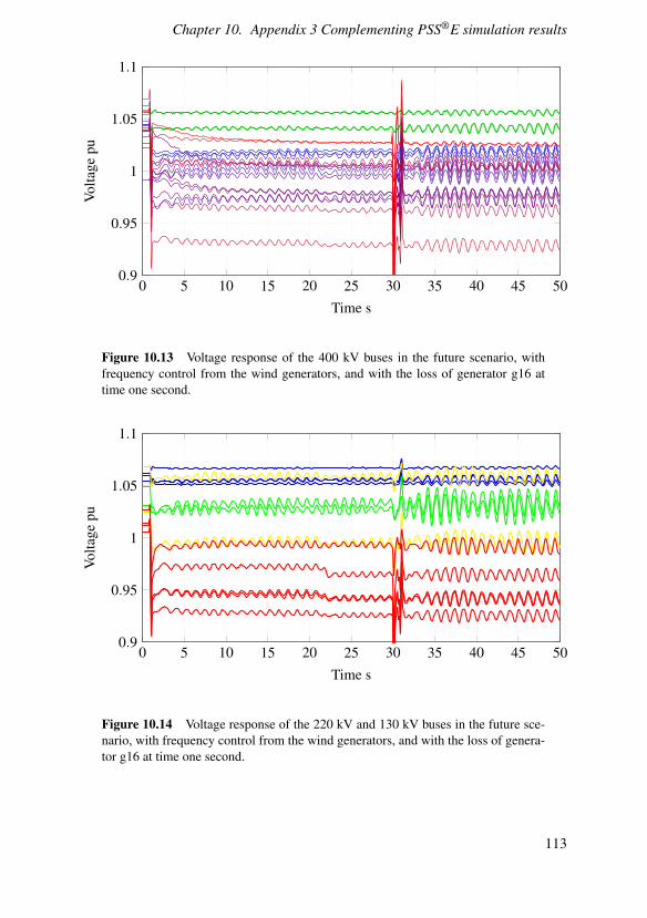
Chapter 10. Appendix 3 Complementing PSS®E simulation results
0 5 10 15 20 25 30 35 40 45 500.9
0.95
1
1.05
1.1
Time s
Volta
gepu
Figure 10.13 Voltage response of the 400 kV buses in the future scenario, withfrequency control from the wind generators, and with the loss of generator g16 attime one second.
0 5 10 15 20 25 30 35 40 45 500.9
0.95
1
1.05
1.1
Time s
Volta
gepu
Figure 10.14 Voltage response of the 220 kV and 130 kV buses in the future sce-nario, with frequency control from the wind generators, and with the loss of genera-tor g16 at time one second.
113

Chapter 10. Appendix 3 Complementing PSS®E simulation results
0 5 10 15 20 25 30 35 40 45 500
5
10
15
20
25
Time s
Act
ive
pow
erpu
Figure 10.15 Active power (in pu on a 100 MVA base) in the different generatorsin the future scenario, with frequency control from the wind generators, with the lossof generator g16 at time one second.
0 5 10 15 20 25 30 35 40 45 50
0
2
4
6
8
Time s
Rea
ctiv
epo
wer
pu
Figure 10.16 Reactive power (in pu on a 100 MVA base) in the different generatorsin the future scenario, with frequency control from the wind generators, with the lossof generator g16 at time one second.
114

Chapter 10. Appendix 3 Complementing PSS®E simulation results
Current day case - loss of generator g9A
0 5 10 15 20 25 30 35 40 45 50−0.3
−0.25
−0.2
−0.15
−0.1
−0.05
0
Time s
Freq
uenc
yde
viat
ion
Hz
Figure 10.17 Frequency response of the 220 kV and 130 kV buses in today’s sce-nario, with the loss of generator g9A at time one second.
115

Chapter 10. Appendix 3 Complementing PSS®E simulation results
0 5 10 15 20 25 30 35 40 45 500.9
0.95
1
1.05
1.1
Time s
Volta
gepu
Figure 10.18 Voltage response of the 400 kV buses in today’s scenario, with theloss of generator g9A at time one second.
0 5 10 15 20 25 30 35 40 45 500.9
0.95
1
1.05
1.1
Time s
Volta
gepu
Figure 10.19 Voltage response of the 220 kV and 130 kV buses in today’s scenario,with the loss of generator g9A at time one second.
116

Chapter 10. Appendix 3 Complementing PSS®E simulation results
0 5 10 15 20 25 30 35 40 45 500
5
10
15
20
25
Time s
Act
ive
pow
erpu
Figure 10.20 Active power (in pu on a 100 MVA base) in the different generatorsin today’s scenario, with the loss of generator g9A at time one second.
0 5 10 15 20 25 30 35 40 45 50
0
2
4
6
8
Time s
Rea
ctiv
epo
wer
pu
Figure 10.21 Reactive power (in pu on a 100 MVA base) in the different generatorsin today’s scenario, with the loss of generator g9A at time one second.
117

Chapter 10. Appendix 3 Complementing PSS®E simulation results
Future scenario - loss of generator g9A with no frequencycontrol from the wind generators
0 5 10 15 20 25 30 35 40 45 50−0.3
−0.25
−0.2
−0.15
−0.1
−0.05
0
Time s
Freq
uenc
yde
viat
ion
Hz
Figure 10.22 Frequency response of the 220 kV and 130 kV buses in the futurescenario, without any frequency control from the wind generators, and with the lossof generator g9A at time one second.
118
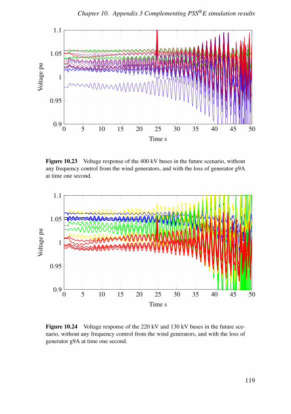
Chapter 10. Appendix 3 Complementing PSS®E simulation results
0 5 10 15 20 25 30 35 40 45 500.9
0.95
1
1.05
1.1
Time s
Volta
gepu
Figure 10.23 Voltage response of the 400 kV buses in the future scenario, withoutany frequency control from the wind generators, and with the loss of generator g9Aat time one second.
0 5 10 15 20 25 30 35 40 45 500.9
0.95
1
1.05
1.1
Time s
Volta
gepu
Figure 10.24 Voltage response of the 220 kV and 130 kV buses in the future sce-nario, without any frequency control from the wind generators, and with the loss ofgenerator g9A at time one second.
119

Chapter 10. Appendix 3 Complementing PSS®E simulation results
0 5 10 15 20 25 30 35 40 45 500
5
10
15
20
25
Time s
Act
ive
pow
erpu
Figure 10.25 Active power (in pu on a 100 MVA base) in the different generatorsin the future scenario, without any frequency control from the wind generators, withthe loss of generator g9A at time one second.
0 5 10 15 20 25 30 35 40 45 50
0
2
4
6
8
Time s
Rea
ctiv
epo
wer
pu
Figure 10.26 Reactive power (in pu on a 100 MVA base) in the different generatorsin the future scenario, without any frequency control from the wind generators, withthe loss of generator g9A at time one second.
120
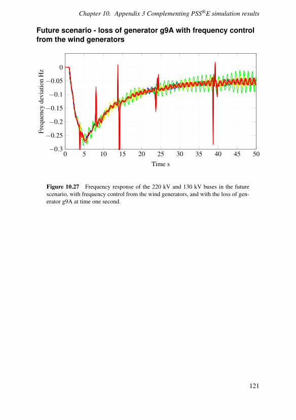
Chapter 10. Appendix 3 Complementing PSS®E simulation results
Future scenario - loss of generator g9A with frequency controlfrom the wind generators
0 5 10 15 20 25 30 35 40 45 50−0.3
−0.25
−0.2
−0.15
−0.1
−0.05
0
Time s
Freq
uenc
yde
viat
ion
Hz
Figure 10.27 Frequency response of the 220 kV and 130 kV buses in the futurescenario, with frequency control from the wind generators, and with the loss of gen-erator g9A at time one second.
121

Chapter 10. Appendix 3 Complementing PSS®E simulation results
0 5 10 15 20 25 30 35 40 45 500.9
0.95
1
1.05
1.1
Time s
Volta
gepu
Figure 10.28 Voltage response of the 400 kV buses in the future scenario, withfrequency control from the wind generators, and with the loss of generator g9A attime one second.
0 5 10 15 20 25 30 35 40 45 500.9
0.95
1
1.05
1.1
Time s
Volta
gepu
Figure 10.29 Voltage response of the 220 kV and 130 kV buses in the future sce-nario, with frequency control from the wind generators, and with the loss of genera-tor g9A at time one second.
122

Chapter 10. Appendix 3 Complementing PSS®E simulation results
0 5 10 15 20 25 30 35 40 45 500
5
10
15
20
25
Time s
Act
ive
pow
erpu
Figure 10.30 Active power (in pu on a 100 MVA base) in the different generatorsin the future scenario, with frequency control from the wind generators, with the lossof generator g9A at time one second.
0 5 10 15 20 25 30 35 40 45 50
0
2
4
6
8
Time s
Rea
ctiv
epo
wer
pu
Figure 10.31 Reactive power (in pu on a 100 MVA base) in the different generatorsin the future scenario, with frequency control from the wind generators, with the lossof generator g9A at time one second.
123


Document name
Date of issue
Document Number
Author(s) Supervisor
Title and subtitle
Abstract
Keywords
Classification system and/or index terms (if any)
Supplementary bibliographical information
ISSN and key title ISBN
Language Number of pages Recipient’s notes
Security classification
Related Documents