Scalability of Planning Before, planning algorithms could synthesize about 6 – 10 action plans in minutes Significant scale-up in the last 6-7 years.

Scalability of Planning

Before, planning algorithms could synthesize about 6 – 10 action plans in minutes

Significant scale-up in the last 6-7 years

Now, we can synthesize 100 action plans in seconds.

Realistic encodings of Munich airport!

The primary revolution in planning in the recent years has been domain-independent heuristics to scale up plan synthesis

Problem is Search Control!!!

…and now for a ring-side retrospective

Relevance, Rechabililty & Heuristics

• Progression takes “applicability” of actions into account

– Specifically, it guarantees that every state in its search queue is reachable

• ..but has no idea whether the states are relevant (constitute progress towards top-level goals)

• SO, heuristics for progression need to help it estimate the “relevance” of the states in the search queue

• Regression takes “relevance” of actions into account

– Specifically, it makes sure that every state in its search queue is relevant

• .. But has not idea whether the states (more accurately, state sets) in its search queue are reachable

• SO, heuristics for regression need to help it estimate the “reachability” of the states in the search queue

Reachability: Given a problem [I,G], a (partial) state S is called reachable if there is a sequence [a1,a2,…,ak] of actions which when executed from state I will lead to a state where S holdsRelevance: Given a problem [I,G], a state S is called relevant if there is a sequence [a1,a2,…,ak] of actions which when executedfrom S will lead to a state satisfying (Relevance is Reachability from goal state)

Since relevance is nothing but reachability from goal state, reachability analysis can form the basis for good heuristics

Reachability through progression

p

pq

pr

ps

pqr

pq

pqs

psq

ps

pst

A1A2

A3

A2A1A3

A1A3

A4

[ECP, 1997]

Planning Graph Basics– Envelope of Progression Tree

(Relaxed Progression)• Linear vs. Exponential Growth

– Reachable states correspond to subsets of proposition lists

– BUT not all subsets are states

• Can be used for estimating non-reachability

– If a state S is not a subset of kth level prop list, then it is definitely not reachable in k steps

p

pq

pr

ps

pqr

pq

pqs

p

psq

ps

pst

pqrs

pqrst

A1A2

A3

A2A1A3

A1A3

A4

A1A2

A3

A1

A2A3A4 [ECP, 1997]

Planning Graph Basics– Envelope of Progression Tree

(Relaxed Progression)• Linear vs. Exponential Growth

– Reachable states correspond to subsets of proposition lists

– BUT not all subsets are states

• Can be used for estimating non-reachability

– If a state S is not a subset of kth level prop list, then it is definitely not reachable in k steps

p

pq

pr

ps

pqr

pq

pqs

p

psq

ps

pst

pqrs

pqrst

A1A2

A3

A2A1A3

A1A3

A4

A1A2

A3

A1

A2A3A4 [ECP, 1997]

Don’t look at curved lines for now…

Have(cake)~eaten(cake)

~Have(cake)eaten(cake)Eat

No-op

No-op

Have(cake)eaten(cake)

bake

~Have(cake)eaten(cake)

Have(cake)~eaten(cake)

Eat

No-op

Have(cake)~eaten(cake)

Graph has leveled off, when the prop list has not changed from the previous iteration

The note that the graph has leveled off now since the last two Prop lists are the same (we could actually have stopped at the

Previous level since we already have all possible literals by step 2)

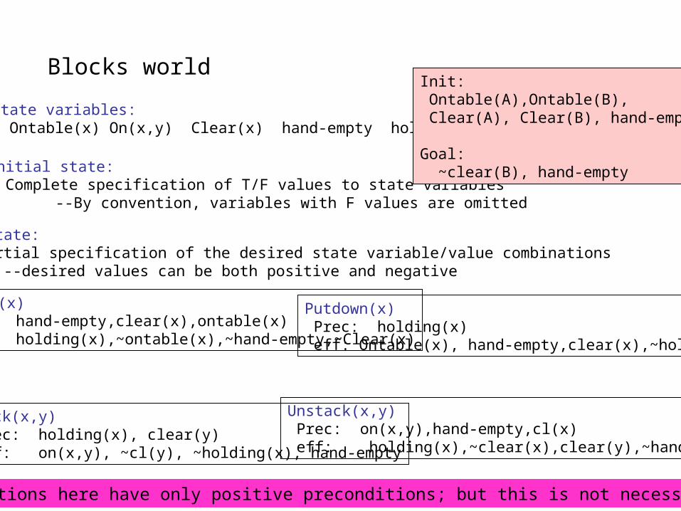
Blocks world

State variables: Ontable(x) On(x,y) Clear(x) hand-empty holding(x)

Stack(x,y) Prec: holding(x), clear(y) eff: on(x,y), ~cl(y), ~holding(x), hand-empty

Unstack(x,y) Prec: on(x,y),hand-empty,cl(x) eff: holding(x),~clear(x),clear(y),~hand-empty

Pickup(x) Prec: hand-empty,clear(x),ontable(x) eff: holding(x),~ontable(x),~hand-empty,~Clear(x)

Putdown(x) Prec: holding(x) eff: Ontable(x), hand-empty,clear(x),~holding(x)

Initial state: Complete specification of T/F values to state variables

--By convention, variables with F values are omitted

Goal state: A partial specification of the desired state variable/value combinations --desired values can be both positive and negative

Init: Ontable(A),Ontable(B), Clear(A), Clear(B), hand-empty

Goal: ~clear(B), hand-empty

All the actions here have only positive preconditions; but this is not necessary

onT-A

onT-B

cl-A

cl-B

he

Pick-A

Pick-B

onT-A

onT-B

cl-A

cl-B

he

h-A

h-B

~cl-A

~cl-B

~he

onT-A

onT-B

cl-A

cl-B

he

Pick-A

Pick-B

onT-A

onT-B

cl-A

cl-B

he

h-A

h-B

~cl-A

~cl-B

~he

St-A-B

St-B-A

Ptdn-A

Ptdn-B

Pick-A

onT-A

onT-B

cl-A

cl-B

he

h-Ah-B

~cl-A

~cl-B

~he

on-A-B

on-B-A

Pick-B

Estimating the cost of achieving individual literals (subgoals)

Idea: Unfold a data structure called “planning graph” as follows:

1. Start with the initial state. This is called the zeroth level proposition list 2. In the next level, called first level action list, put all the actions whose preconditions are true in the initial state -- Have links between actions and their preconditions 3. In the next level, called first level propostion list, put: Note: A literal appears at most once in a proposition list. 3.1. All the effects of all the actions in the previous level. Links the effects to the respective actions. (If multiple actions give a particular effect, have multiple links to that effect from all those actions) 3.2. All the conditions in the previous proposition list (in this case zeroth proposition list). Put persistence links between the corresponding literals in the previous proposition list and the current proposition list.*4. Repeat steps 2 and 3 until there is no difference between two consecutive proposition lists. At that point the graph is said to have “leveled off”

The next 2 slides show this expansion upto two levels

Using the planning graph to estimate the cost of single literals:

1. We can say that the cost of a single literal is the index of the first proposition level in which it appears. --If the literal does not appear in any of the levels in the currently expanded planning graph, then the cost of that literal is: -- l+1 if the graph has been expanded to l levels, but has not yet leveled off -- Infinity, if the graph has been expanded (basically, the literal cannot be achieved from the current initial state)

Examples: h({~he}) = 1 h ({On(A,B)}) = 2 h({he})= 0

How about sets of literals? see next slide

onT-A

onT-B

cl-A

cl-B

he

Pick-A

Pick-B

onT-A

onT-B

cl-A

cl-B

he

h-A

h-B

~cl-A

~cl-B

~he

St-A-B

St-B-A

Ptdn-A

Ptdn-B

Pick-A

onT-A

onT-B

cl-A

cl-B

he

h-Ah-B

~cl-A

~cl-B

~he

on-A-B

on-B-A

Pick-B

Estimating reachability of sets

We can estimate cost of a set of literals in three ways:• Make independence assumption

• H(p,q,r)= h(p)+h(q)+h(r) • if we define the cost of a set of literals in terms

of the level where they appear together• h-lev({p,q,r})= The index of the first level of the PG where

p,q,r appear together• so, h({~he,h-A}) = 1

• Compute the length of a “relaxed plan” to supporting all the literals in the set S, and use it as the heuristic (**) hrelax

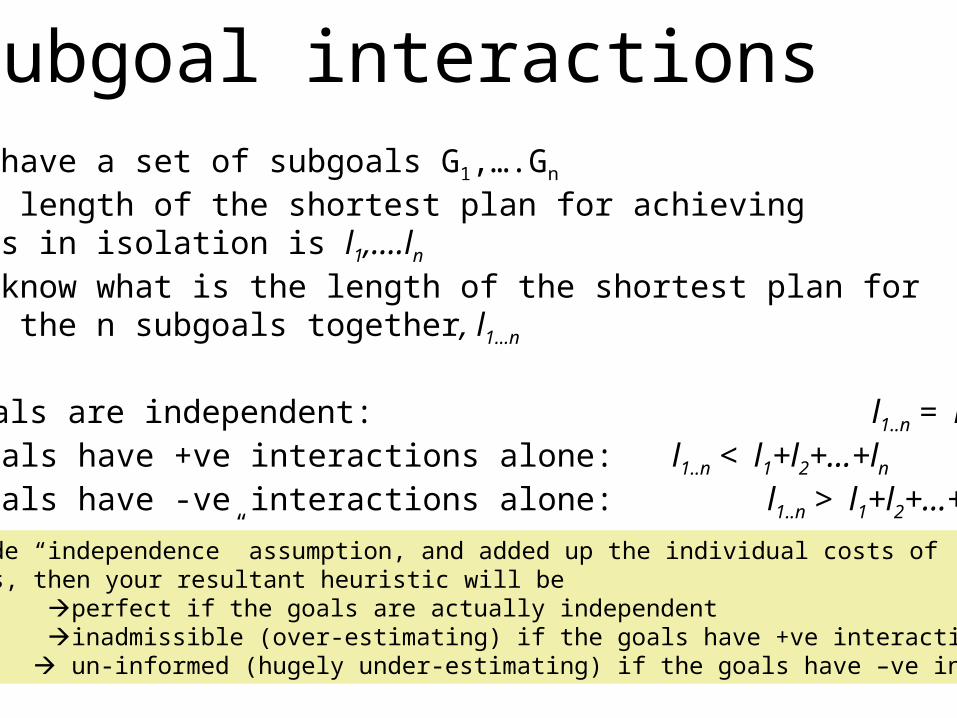
Subgoal interactionsSuppose we have a set of subgoals G1,….Gn

Suppose the length of the shortest plan for achieving the subgoals in isolation is l1,….ln We want to know what is the length of the shortest plan for achieving the n subgoals together, l1…n

If subgoals are independent: l1..n = l1+l2+…+ln If subgoals have +ve interactions alone: l1..n < l1+l2+…+ln If subgoals have -ve interactions alone: l1..n > l1+l2+…+ln

If you made “independence” assumption, and added up the individual costs of subgoals, then your resultant heuristic will be perfect if the goals are actually independent inadmissible (over-estimating) if the goals have +ve interactions un-informed (hugely under-estimating) if the goals have –ve interactions

“Relaxed plan”• Suppose you want to find a relaxed

plan for supporting literals g1…gm on a k-length PG. You do it this way:

– Start at kth level. Pick an action for supporting each gi (the actions don’t have to be distinct—one can support more than one goal). Let the actions chosen be {a1…aj}

– Take the union of preconditions of a1…aj. Let these be the set p1…pv.

– Repeat the steps 1 and 2 for p1…pv—continue until you reach init prop list.

• The plan is called “relaxed” because you are assuming that sets of actions can be done together without negative interactions.

onT-A

onT-B

cl-A

cl-B

he

Pick-A

Pick-B

onT-A

onT-B

cl-A

cl-B

he

h-A

h-B

~cl-A

~cl-B

~he

St-A-B

St-B-A

Ptdn-A

Ptdn-B

Pick-A

onT-A

onT-B

cl-A

cl-B

he

h-Ah-B

~cl-A

~cl-B

~he

on-A-B

on-B-A

Pick-B

No backtracking needed!

Optimal relaxed plan is still NP-hard

onT-A

onT-B

cl-A

cl-B

he

Pick-A

Pick-B

onT-A

onT-B

cl-A

cl-B

he

h-A

h-B

~cl-A

~cl-B

~he

St-A-B

St-B-A

Ptdn-A

Ptdn-B

Pick-A

onT-A

onT-B

cl-A

cl-B

he

h-Ah-B

~cl-A

~cl-B

~he

on-A-B

on-B-A

Pick-B

Relaxed plan for our blocks example

h-ind; h-lev; h-relax

• H-lev is lower than or equal to h-relax

• H-ind is larger than or equal to H-lev

• H-lev is admissible

• H-relax is not admissible unless you find optimal relaxed plan– Which is NP-Hard..

Planning Graphs for heuristics

Construct planning graph(s) at each search node Extract relaxed plan to achieve goal for

heuristic

p5

q5

r5

p6

opq

opr

o56

p

5

pqr56

opq

opr

o56

pqrst567

ops

oqt

o67

q

5

qtr56

oqt

oqr

o56

qtrsp567

oqs

otp

o67r

5

rqp56

orq

orp

o56

rqpst567

ors

oqt

o67p

6

pqr67

opq

opr

o67

pqrst678

ops

oqt

o78

1

3

4

1

3

o12

o34

2

1

3

4

5

o12

o34

o23

o45

2

3

4

5

3

5

o34

o56

3

4

5

o34

o45

o56

6 6

7

o67

1

5

1

5

o12

o56

2

1

3

5

o12

o23

o56

2

6 6

7

o67

GoG

GoG

GoG

GoG

GoG

1

3

3

5

1

5

h( )=5

--4/19 lecture ended here--

Slides beyond this were not discussed in the class

onT-A

onT-B

cl-A

cl-B

he

Pick-A

Pick-B

onT-A

onT-B

cl-A

cl-B

he

h-A

h-B

~cl-A

~cl-B

~he

St-A-B

St-B-A

Ptdn-A

Ptdn-B

Pick-A

onT-A

onT-B

cl-A

cl-B

he

h-Ah-B

~cl-A

~cl-B

~he

on-A-B

on-B-A

Pick-B

onT-A

onT-B

cl-A

cl-B

he

Pick-A

Pick-B

onT-A

onT-B

cl-A

cl-B

he

h-A

h-B

~cl-A

~cl-B

~he

St-A-B

St-B-A

Ptdn-A

Ptdn-B

Pick-A

onT-A

onT-B

cl-A

cl-B

he

h-Ah-B

~cl-A

~cl-B

~he

on-A-B

on-B-A

Pick-B

onT-A

onT-B

cl-A

cl-B

he

Pick-A

Pick-B

onT-A

onT-B

cl-A

cl-B

he

h-A

h-B

~cl-A

~cl-B

~he

St-A-B

St-B-A

Ptdn-A

Ptdn-B

Pick-A

onT-A

onT-B

cl-A

cl-B

he

h-Ah-B

~cl-A

~cl-B

~he

on-A-B

on-B-A

Pick-B

onT-A

onT-B

cl-A

cl-B

he

Pick-A

Pick-B

onT-A

onT-B

cl-A

cl-B

he

h-A

h-B

~cl-A

~cl-B

~he

St-A-B

St-B-A

Ptdn-A

Ptdn-B

Pick-A

onT-A

onT-B

cl-A

cl-B

he

h-Ah-B

~cl-A

~cl-B

~he

on-A-B

on-B-A

Pick-B

Progression Regression

How do we use reachability heuristics for regression?

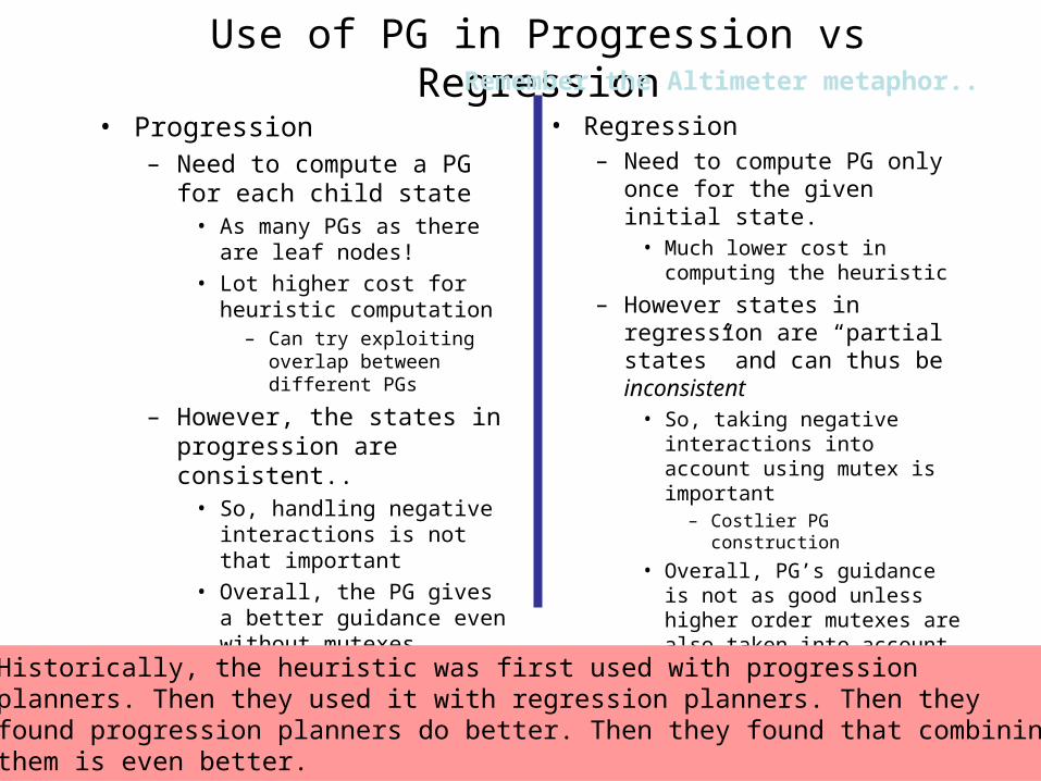
Use of PG in Progression vs Regression

• Progression– Need to compute a PG for

each child state• As many PGs as there are

leaf nodes!• Lot higher cost for heuristic

computation– Can try exploiting overlap

between different PGs

– However, the states in progression are consistent..

• So, handling negative interactions is not that important

• Overall, the PG gives a better guidance even without mutexes

• Regression– Need to compute PG only

once for the given initial state.

• Much lower cost in computing the heuristic

– However states in regression are “partial states” and can thus be inconsistent

• So, taking negative interactions into account using mutex is important

– Costlier PG construction

• Overall, PG’s guidance is not as good unless higher order mutexes are also taken into accountHistorically, the heuristic was first used with progression

planners. Then they used it with regression planners. Then theyfound progression planners do better. Then they found that combining them is even better.

Remember the Altimeter metaphor..

What if actions have non-uniform costs?

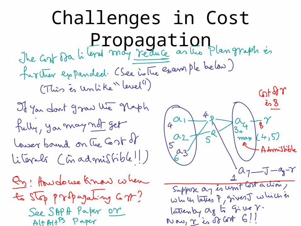
Challenges in Cost Propagation

Cost of a set of literals?

• We can compute a relaxed plan to support those literals– It is clear now that optimal relaxed plan will be

NP-hard– Greedy approaches could be used

• Support the goals using the actions that have the lowest propagated cost

PGs for reducing actions

• If you just use the action instances at the final action level of a leveled PG, then you are guaranteed to preserve completeness

– Reason: Any action that can be done in a state that is even possibly reachable from init state is in that last level

– Cuts down branching factor significantly

– Sometimes, you take more risky gambles:• If you are considering the goals {p,q,r,s}, just look at the actions that appear

in the level preceding the first level where {p,q,r,s} appear for the first time without Mutex.

Negative Interactions• To better account for -ve interactions, we need to start looking into

feasibility of subsets of literals actually being true together in a proposition level.

• Specifically,in each proposition level, we want to mark not just which individual literals are feasible, – but also which pairs, which triples, which quadruples, and which

n-tuples are feasible. (It is quite possible that two literals are independently feasible in level k, but not feasible together in that level)

• The idea then is to say that the cost of a set of S literals is the index of the first level of the planning graph, where no subset of S is marked infeasible

• The full scale mark-up is very costly, and makes the cost of planning graph construction equal the cost of enumerating the full progres sion search tree.

– Since we only want estimates, it is okay if talk of feasibility of upto k-tuples• For the special case of feasibility of k=2 (2-sized subsets), there are

some very efficient marking and propagation procedures. – This is the idea of marking and propagating mutual exclusion relations.

Don’t look at curved lines for now…

Have(cake)~eaten(cake)

~Have(cake)eaten(cake)Eat

No-op

No-op

Have(cake)eaten(cake)

bake

~Have(cake)eaten(cake)

Have(cake)~eaten(cake)

Eat

No-op

Have(cake)~eaten(cake)

Graph has leveled off, when the prop list has not changed from the previous iteration

The note that the graph has leveled off now since the last two Prop lists are the same (we could actually have stopped at the

Previous level since we already have all possible literals by step 2)

Level-off definition? When neither propositions nor mutexes change between levels

•Rule 1. Two actions a1 and a2 are mutex if

(a)both of the actions are non-noop actions or

(b) a1 is any action supporting P, and a2 either needs ~P, or gives ~P.

(c) some precondition of a1 is marked mutex with some precondition of a2

Rule 2. Two propositions P1 and P2 are marked mutex if all actions supporting P1 are pair-wise mutex with all actions supporting P2.

Mutex Propagation Rules

Serial graph

interferene

Competing needs

This one is not listed in the text

onT-A

onT-B

cl-A

cl-B

he

Pick-A

Pick-B

onT-A

onT-B

cl-A

cl-B

he

h-A

h-B

~cl-A

~cl-B

~he

onT-A

onT-B

cl-A

cl-B

he

Pick-A

Pick-B

onT-A

onT-B

cl-A

cl-B

he

h-A

h-B

~cl-A

~cl-B

~he

St-A-B

St-B-A

Ptdn-A

Ptdn-B

Pick-A

onT-A

onT-B

cl-A

cl-B

he

h-Ah-B

~cl-A

~cl-B

~he

on-A-B

on-B-A

Pick-B

Level-based heuristics on planning graph with mutex relations

hlev({p1, …pn})= The index of the first level of the PG where p1, …pn appear together and no pair of them are marked mutex. (If there is no such level, then hlev is set to l+1 if the PG is expanded to l levels, and to infinity, if it has been expanded until it leveled off)

We now modify the hlev heuristic as follows

This heuristic is admissible. With this heuristic, we have a much better handle on both +ve and -ve interactions. In our example, this heuristic gives the following reasonable costs:

h({~he, cl-A}) = 1h({~cl-B,he}) = 2 h({he, h-A}) = infinity (because they will be marked mutex even in the final level of the leveled PG)

Works very well in practice

H({have(cake),eaten(cake)}) = 2