Scalability of an Unstructured Grid Continuous Galerkin Based Hurricane Storm Surge Model

Scalability of an Unstructured GridContinuous Galerkin Based Hurricane Storm

Surge Model

S. Tanaka1)∗, S. Bunya2), J.J. Westerink3), C. Dawson4),R.A. Luettich, Jr.5)

1) Assistant Research Professor,

Environmental Fluid Dynamics Laboratories,

Department of Civil Engineering and Geological Sciences,

University of Notre Dame, Notre Dame, IN, U.S.A.2) Consultant, Science and Safety Policy Research Division,

Mitsubishi Research Institute, Inc.,

Chiyoda-ku, Tokyo, Japan3) Professor, Environmental Fluid Dynamics Laboratories,

Department of Civil Engineering and Geological Sciences,

University of Notre Dame, Notre Dame, IN, U.S.A.4) Professor, Institute for Computational Engineering and Sciences,

The University of Texas at Austin, Austin, TX, U.S.A.5) Professor, Institute of Marine Sciences,

University of North Carolina at Chapel Hill,

Morehead City, NC, U.S.A.

Running Head:Scalability of Continuous Galerkin Based Hurricane Storm

Surge Model

SubmittedJanuary 20, 2010

In Revised FormJune 22, 2010

Journal of Scientific Computing

∗Corresponding author: Seizo Tanaka,Environmental Fluid Dynamics Laboratories,Department of Civil Engineering and Geological Sciences,156 Fitzpatrick Hall, Notre Dame, IN, 46556, U.S.A.,tel:(574)631-3864, fax:(574)631-9236,e-mail: [email protected]

1

Abstract

This paper evaluates the parallel performance and scalability of an

unstructured grid Shallow Water Equation (SWE) hurricane storm

surge model. We use the ADCIRC model, which is based on the

generalized wave continuity equation continuous Galerkin method,

within a parallel computational framework based on domain decom-

position and the MPI (Message Passing Interface) library. We mea-

sure the performance of the model run implicitly and explicitly on

various grids. We analyze the performance as well as accurracy with

various spatial and temporal discretizations. We improve the output

writing performance by introducing sets of dedicated writer cores.

Performance is measured on the Texas Advanced Computing Center

Ranger machine. A high resolution 9,314,706 finite element node grid

with 1s time steps can complete a day of real time hurricane storm

surge simulation in less than 20 min of computer wall clock time, us-

ing 16,384 cores with sets of dedicated writer cores.

Keywords : parallel computing, scaling, shallow water equations,

hurricane storm surge model, finite element method, forecasting

2

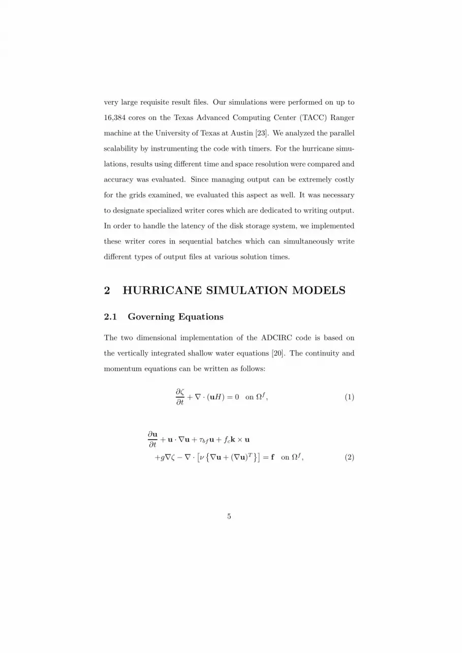
1 INTRODUCTION

Hurricane storm surge is a low probabity but high impact disaster that

can result in massive destruction of coastal infrastructure and significant

loss of human life. Recent storms such as Katrina (2005), Rita (2005), Ike

(2008) and Nargis (2008) have led to devastating damage. Hurricane storm

surge and the resulting water levels and currents involve a wide range of

processes as well as scales. Storm surge is regionally and locally generated

in the coastal ocean, in inland waterbodies and over coastal floodplains

and moves through rivers, inlets and channels. Storm surge is driven and

affected by tides, river flows, wind waves, winds and atmospheric pressure.

The simulation of hurricane storm surge is a powerful tool used to evalu-

ate risk, design hurricane protection systems, analyze the physics of storms,

and plan evacuations [1]. These simulations must be fast and accurate in

order to estimate the water level and current environment and assess the

potential of risk and damage. In particular, within the realm of forcasting,

two to four days of real time simulation must be completed within an hour

of computer wall clock time in order to be useful to emergency planners.

However, realistic solutions require the use of high resolution computa-

tional grids that express complicated domain shapes, detailed topography,

geographical features, bathymetry and flow structures. High resolution

grids require significant memory and computational time. The rapid de-

velopment of multi-CPU/core parallel architectures with fast networks has

dramatically improved the potential for large scale simulations with fast

turnaround. In order to take advantage of these parallel computational

platforms, it is critical that the computations be scalable. As we increase

3

the number of cores, we must consider both the time of the computation

and the time required for managing and processing the necessary output

files.

The ADCIRC model has been extensively used to model hurricane storm

surge along the U.S. East and Gulf coasts by the U.S. Army Corps of

Engineers and the Federal Emergency Management Agency for the devel-

opment of flood risk mitigation systems, flood risk evaluation, and surge

forecasting. ADCIRC, a community developed model, is a two and three

dimensional coastal ocean hydrodynamic model implemented using both

continuous Galerkin (CG) and discontinuous Galerkin (DG) finite element

solutions [2]-[15]. The application of basin to channel scale domains using

unstructured grids with highly localized resolution is ideal for modeling

the riverine, tidal, wind wave, wind, and atmospheric pressure driven flows

during a hurricane event. The resulting solutions are both accurate and

robust on a wide range of scales and flow phenomena [16]-[22]. For these

high resolution computations, ADCIRC has been implemented in paral-

lel using domain decomposition and the MPI (Message Passing Interface)

communication library.

In this paper, we report on the scalability of CG based explicit and

implicit implementations of ADCIRC in two space dimensions when com-

puting tides and storm surge using large high resolution grids. The number

of finite element nodes for the cases examined varies between 254,565 and

9,314,706, with three degrees of freedom computed at every finite element

node every 0.5 second to 2 seconds. We measure parallel scalability on

different resolution grids, compare temporal and spatial accuracy for both

the implicit and explicit solutions, and evaluate the costs of outputting the

4

very large requisite result files. Our simulations were performed on up to

16,384 cores on the Texas Advanced Computing Center (TACC) Ranger

machine at the University of Texas at Austin [23]. We analyzed the parallel

scalability by instrumenting the code with timers. For the hurricane simu-

lations, results using different time and space resolution were compared and

accuracy was evaluated. Since managing output can be extremely costly

for the grids examined, we evaluated this aspect as well. It was necessary

to designate specialized writer cores which are dedicated to writing output.

In order to handle the latency of the disk storage system, we implemented

these writer cores in sequential batches which can simultaneously write

different types of output files at various solution times.

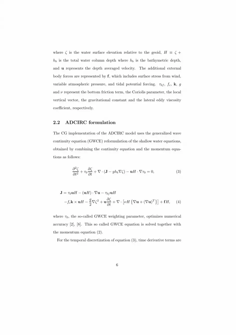
2 HURRICANE SIMULATION MODELS

2.1 Governing Equations

The two dimensional implementation of the ADCIRC code is based on

the vertically integrated shallow water equations [20]. The continuity and

momentum equations can be written as follows:

∂ζ

∂t+ ∇ · (uH) = 0 on Ωf , (1)

∂u

∂t+ u · ∇u + τbfu + fck × u

+g∇ζ −∇ ·[

ν

∇u + (∇u)T]

= f on Ωf , (2)

5

where ζ is the water surface elevation relative to the geoid, H ≡ ζ +

hb is the total water column depth where hb is the bathymetric depth,

and u represents the depth averaged velocity. The additional external

body forces are represented by f , which includes surface stress from wind,

variable atmospheric pressure, and tidal potential forcing. τbf , fc, k, g

and ν represent the bottom friction term, the Coriolis parameter, the local

vertical vector, the gravitational constant and the lateral eddy viscosity

coefficient, respectively.

2.2 ADCIRC formulation

The CG implementation of the ADCIRC model uses the generalized wave

continuity equation (GWCE) reformulation of the shallow water equations,

obtained by combining the continuity equation and the momentum equa-

tions as follows:

∂2ζ

∂t2+ τ0

∂ζ

∂t+ ∇ · (J − ghb∇ζ) − uH · ∇τ0 = 0, (3)

J = τ0uH − (uH) · ∇u − τbfuH

−fck × uH −g

2∇ζ2 + u

∂ζ

∂t+ ∇ ·

[

νH

∇u + (∇u)T]

+ fH, (4)

where τ0, the so-called GWCE weighting parameter, optimizes numerical

accuracy [2], [8]. This so called GWCE equation is solved together with

the momentum equation (2).

For the temporal discretization of equation (3), time derivative terms are

6

treated as follows:

∂2ζ

∂t2=

ζn+1− 2ζn + ζn−1

∆t2, (5)

∂ζ

∂t=

ζn+1− ζn−1

2∆t, (6)

where n denotes the time level and ∆t is the time step size. The variable

ζ is weighted over three time levels as follows:

ζ = α1ζn+1 + α2ζ

n + α3ζn−1, (7)

α1 + α2 + α3 = 1, (8)

where αi is a parameter to control acurracy and stability. The variables J,

u, f are treated explicitly as known terms in this time step level [8].

The temporal discretization of momentum equation (2) is explicit except

for the Coriolis term. The time derivative term and velocity in the bottom

friction term and Coriolis force term are treated as:

∂u

∂t=

un+1

− un

∆t, (9)

u =1

2

(

un+1 + u

n)

. (10)

The standard Galerkin finite element method is applied for the spatial

discretization of equations (3) and (2). The linear C0 continuous element

7

is used for both ζ and u.

After the discretization for time and space above, we obtain the following

set of linear equations:

(

1

∆t2M +

1

2∆tM τ0

+ α1Dhb

)

∆Zn+1

=

(

1

∆t2M −

1

2∆tM τ0

− (α1 + α2)Dhb

)

∆Zn

+ DhbZ

n−1 + Zn, (11)

(

1

∆t+

τbf

2

)

MLUn+1 +

fc

2ML

(

k × Un+1

)

=

(

1

∆t−

τbf

2

)

MLUn−

fc

2ML (k × U

n) + Un, (12)

where Z, U represent the nodal vector(s) of ζ, u. ∆(:)n+1 indicates the

difference on this time step level. Zn, U

n are known nodal vectors on

this time level. Normally, we solve the GWCE implicitly and we set the

temporal control parameters to α1 = α2 = α3 = 13 . Equation (11) is solved

using a conjugate gradient iterative solver with diagonal scaling system

based on Compressed Row Storage (CRS) [24]. The discrete momentum

equations (12) are solved explicitly and apply a lumped mass matrix, ML,

and are therefore matrix free. Details are discussed in [8]. We designate

this scheme as the implicit solution in this paper. On the other hand, if

we set the temporal control parameters in equation (11) to α1 = α3 = 0,

α2 = 1, we can solve the discrete GWCE system explicitly using the lumped

mass matrix in the GWCE. This results in an entirely matrix free solution

for both ζ and u, reducing both computational time and memory. We

designate this as the explicit solution.

8

2.3 Code parallelization

The ADCIRC parallel computation is based on a domain decomposition

paradigm. The computational domain is divided into sub-domains with

one overlapping layer of finite elements between adjacent sub-domains as

shown as Figure 1. Each sub-domain is allocated to an individual core.

METIS [25], which is based on graph theory, is used as the domain de-

composer. For the parallel computation, two types of inter-subdomain and

inter-core communication are required. Communication is necessary be-

tween the neighboring sub-domains to complete the correct assembly of

the subdomain nodal matrices and vectors and to ensure that all subdo-

main vectors match the global vectors. The data on the inside node of the

overlapping layer is sent to the neighboring sub-domain, and the data on

the external edge of the layer is received from the neighboring sub-domain.

In addition, communication among all sub-domains is required to calculate

a summation over the entire global domain. This communication step is

necessary for the dot product in the iterative solver in order to evaluate

the residual norm of the solution. There are two dot products in each

conjugate gradient iteration and generally 10-15 iterations are required to

reach convergence. Therefore, the implicit solution requires 20 to 30 global

communication procedures in one time step. On the other hand, this global

communication procedure does not appear in the explicit solution.

For these communications, MPI (Message Passing Interface) is used.

Specifically for communication between adjacent subdomains, MPI ISEND

and MPI IRECV are used in both the implicit and explicit solution, while

MPI ALLREDUCE is used for the necessary global communication for the

9

https://www.researchgate.net/publication/202924228_Multilevel_k-way_Partitioning_Scheme_for_Irregular_Graphs?el=1_x_8&enrichId=rgreq-699a7a74-3ee1-4933-8981-f4fa921f9a77&enrichSource=Y292ZXJQYWdlOzIyNTQxNzM5MTtBUzoxMDI2NTUxMTIyNTM0NTVAMTQwMTQ4NjI5NTg0Mg==

implicit solution.

2.4 Application of sequential batches of dedicated writer

cores

Our standard implementation of managing output simply consists of a glob-

alization process of output from all cores to core number 0 (C0) which then

writes the information to the disk storage system. On machines such as the

CRAY XT3 (Sapphire, [26]) and the CRAY XT4 (Jade, [27]), the procedure

works well, largely due to the high level output caching and output data

management by the operating system. On TACC’s Lonestar and Ranger

machines, the standard output procedure takes considerable time, often

more than doubling the wall clock time. The problem is that the output

file data is as large as approximately 100 Bytes per finite element node

per output time interval, which amounts to approximately 1.0 GBytes per

output time interval for a grid with 9,314,706 nodes when writing surface

water elevations, water velocities, atmospheric pressure, and wind speeds.

A typical output time interval is 15 to 30 minutes. The time required to

write this data to the disk array is large, sometimes substantially exceed-

ing the actual computational time required between output time intervals.

The problem is aggravated when using large numbers of cores.

Figure 2 shows the time schedule for the computation and writing proce-

dure using the standard output procedure for two output files. All cores are

compute cores, and the results of each sub-domain are gathered to compute

core number 0 (C0). Core C0 then outputs the result to the disk storage

system. The other compute cores can not proceed to the next time step

10

until core C0 finishes writing the results.

We therefore investigated the use of dedicated writer cores to reduce the

total wall clock time for the simulation which includes the computation time

in addition to the required file writing time. The specialized writer cores

do not handle any portion of the actual finite element computation and

have no assigned sub-domain. These cores devote themselves to collecting

the output data from all the compute cores, globalizing the necessary files

and then writing these files to the disk storage system.

The time schedule of the dedicated writer core algorithm is shown in

Figure 3. The compute cores can move to the next step immediately after

they have sent their results to the specialized writer cores. We can have

one writer core handling all output files, or one writer core per output

file, effectively distributing the output load. The writer cores output the

results to the disk array while the compute cores proceed with the finite

element computation. If the output time is longer than the simulation

time, the compute cores do have to wait until the writer cores finish writing

because the compute cores cannot send their data. For this situation, we

simply have to use a larger total number of writer cores than the number

of output files. Figure 4 shows a case with four writer cores for two output

files. Defining the sequential batches of writer cores allows each batch

to complete the writing process over several writing output time intervals.

When a batch of writer cores completes the writing procedure, they become

available to handle another set of output files. The compute cores can send

the result data to the next batch of writer cores without stopping.

We note that for all implementations of the dedicated writer cores, the

time required to send data to the appropriate writer cores interrupts the

11

computation. However the computation is not slowed down by the time

needed to do the actual writing to the disk storage system, which is sub-

stantially longer than the data collection and globalization time.

2.5 Flow of the computation

The flow chart of the computation is shown in Figure 5. The computation

during a time step can be detailed as follows:

1) The left hand side matrix and right hand side vector of equation (11)

are calculated and solved using a conjugate gradient method in the

implicit solution. For the explicit solution, the left hand side matrix

uses a lumped mass matrix (i.e. terms only on the diagonal) and is

therefore matrix free.

2) If the domain has a lateral moving boundary, a wet/dry judgment is

required to update the active wet finite elements. For the implicit

solution, a global Allreduce is required to determine if elements have

changed from wet to dry or dry to wet so that this information can

be used to reconstruct and solve the global matrix. No such call is

necessary for the explicit solution.

3) The right hand side vector of equation (12) is calculated and the

system is solved using a lumped mass matrix, resulting in a matrix

free solution for velocity.

4) The computed results are output to the disk storage system at re-

quired output intervals.

5) The time step loop 1)∼4) is repeated until the final time step.

12

2.6 Computer system specifications

We used the Sun Blade cluster based supercomputer Ranger at TACC at

the University of Texas at Austin [23]. Ranger has 3,936 compute nodes,

each node has four quadcore AMD Opteron 8356 processors for a total of

62,976 cores. All compute nodes are interconnected with a 1GB/s Infini-

Band network. The specifications of each compute node are shown in Table

1. CentOS 4.8(x86 64) is used as the operating system, and we used PGI

Fortran 4.2.1 and MVAPICH 1.0 as the Fortran compiler and MPI Library.

3 Performance Benchmarks

3.1 Benchmark problems

We used two different base grids in order to evaluate the performance of

both the implicit and explicit implementation of the CG GWCE based AD-

CIRC solution. The first is the SL15 grid which was developed to evaluate

tidal, riverine, wind wave and hurricane induced storm surge response in

coastal Louisiana and Mississippi [21][22]. The model applies a finite ele-

ment grid with elements that range between 30m and 24km. The model

considers finite elements changing from wet to dry or dry to wet states

simulating a lateral wetting and drying moving boundary. In addition,

the model incorporates flow overtopping weirs handled as internal barrier

boundaries. The second grid is the EC2001 model which was developed to

study tides in the western North Atlantic, Gulf of Mexico and Caribbean

Sea and applies finite elements ranging between 150m and 24km [19]. The

EC2001 model does not include the wetting and drying process or internal

13

barrier boundaries.

The SL15x01 grid, shown in Figure 6, applies large elements in deep

ocean water, an intermediate level of resolution on continental shelves and

a high level of resolution in coastal Louisiana and Mississippi, the region

of specific interest. Figure 6 also shows a sample domain decomposition,

the bold lines designating the borders of the 1,024 sub-domains. The areal

extent of the sub-domains varies dramatically and is inversely proportional

to grid size. The EC2001 grid, shown in Figure 7, shows less variabil-

ity in grid size and therefore more uniformity in the areal coverage of the

sub-domains. We refined these two base grids into higher resolution im-

plementations by dividing the base grid elements into 4 and 16 elements

as illustrated in Figure 8. We use x01, x04 and x16 as suffixes of the grid

names to differentiate the grids with the original and indicate the level of

increased resolution. The grids and the total number of nodes and elements

are summarized in Table 2.

In order to study CG ADCIRC’s parallel performance and scalability,

tidal simulations were performed on the SL15x01, x04 and the EC2001x01,

x04, x16 grids. Hurricane storm surge simulations were carried out for

the SL15x01, x04 grids to quantify temporal and spatial accuracy and

to compare the results of the implicit and explicit solutions. The latter

simulations were also used to quantify the performance of the standard

output and dedicated writer core output options.

3.2 Parallel performance

In order to measure the parallel performance of the CG implementation of

ADCIRC, tidal flow simulations were carried out on Ranger. Output file

14

writing was suppressed for these simulations. We measured the wall clock

time using 16 to 16,384 cores for 6 hours of real time simulation. A time

step, ∆t = 1s was used for the SL15x01 grid, and 0.5s was used for the

SL15x04 grid in order to maintain stability as well as accuracy. Table 3

summarizes runtime information for the implicit and the explicit solutions

on the SL15x01 and SL15x04 grids. The wall clock times presented in this

table and the related figures are normalized to 1day of simulation using a

1s time step. Figure 9 shows a comparison of the wall clock times of the

implicit and the explicit solutions for both grids as a function of the total

number of cores. We can see that wall clock time is inversely proportional

to the number of cores over a wide range of cores. We note that the slopes of

these curves often exceed the ideal slope of minus one over a range of cores.

This is largely related to caching efficiencies which are most consistently

noted in the increased rate of scaling between 256 and 512 cores for both

the implicit and explicit solutions of the SL15x01 grid, and between 1024

and 2048 cores for the implicit and explicit solutions of the SL15x04 grid.

Ultimately the ideal scaling on all the grids is lost although this occurs

later for the larger SL15x04 grid and also occurs later and more slowly for

the explicit solution as compared to the implicit solution. Furthermore, we

note that the explicit solution is about twice as fast as the implicit solution

on a per time step basis from a small number of cores until the curves start

to tail off, at which point the difference becomes larger.

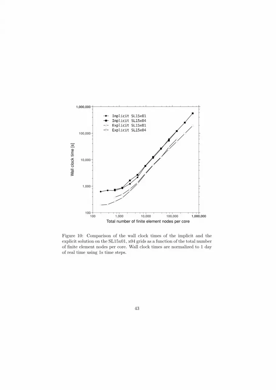
Figure 10 highlights these features by plotting wall clock times against

the number of finite element nodes per core. Again the wall clock time

is normalized to 1day of simulation using a 1s time step. We note that

now the performance of the SL15x01 and SL15x04 grids is very similar for

15

the implicit solution as it is for the explicit solution. Overall performance

appears to be controlled by the number of finite element nodes per core for

each of these solutions. We note approximately ideal scaling for all solutions

with the better than ideal scaling between 4,500 and 9,000 finite element

nodes per core, corresponding to the aforementioned caching efficiencies.

Degradation in ideal scaling occurs quite rapidly for the implicit solution

at about 2,200 finite element nodes per core and much more slowly for the

explicit solution at about 1,100 finite element nodes per core. Thus both

solutions exhibit weak scaling, i.e. the implicit solutions for the two grids

overlay each other as do the explicit solutions. Furthermore, strong scaling

characteristics for individual solutions are sustained until about 1,100 to

2,200 finite element nodes per core although the degradation in ideal scaling

is much slower for the explicit solution.

Figure 11 shows the parallel speedup obtained when doubling the number

of cores in intervals between 16 and 16,384 plotted as a function of the total

number of finite element nodes per core. Parallel speedup achieved when

doubling the number of cores is defined as:

Parallel SpeedupN2c=

TimeNc

TimeN2c

, (13)

where Nc is the total number of cores and N2c is twice the number of cores.

The ideal parallel speedup is equal to 2.0. Between 300,000 and 10,000 finite

element nodes per core, the ideal speedup is achieved and often episodically

improved upon, due to improvements in caching and memory access. At

4500 finite element nodes per core, reflecting the scaling between 9000 and

4500 finite element nodes per core, we note a consistent boost beyond

16

ideal speedup for all solutions, reflecting significant improvements in cache

utilization that occur in this range of finite element nodes per core. For

fewer than 2,200 finite element nodes per core, a degradation in efficiency

occurs at various rates.

A detailed analysis of the core utilization for the SL15x04 grid is pre-

sented for the implicit and explicit solution in Figure 12 and 13 respec-

tively. The total wall clock time, the wall clock time of the solution of

the continuity equation, the momentum equations, the wetting and dry-

ing judgment, the local communication (Send and Receive), and the global

communication (Allreduce) are shown for the implicit solution as a func-

tion of the total number of cores. Identical information is shown for the

explicit solution with the exception of the global communication time which

is not required for the explicit solution. We note that for the implicit so-

lution both the total solution time, continuity equation solution time and

the wetting/drying judgment exhibit degradation in scalability with large

numbers of cores while the momentum equation solution sees only a mod-

est reduction in scalability at 8,192 cores. More importantly while the

local communication sees some limited growth at 4,096 cores, the global

communication time sees steady increases over the entire range of cores.

In fact, the global communication time becomes a dominating contributor

to the total time as the total number of cores grows. We note that there

may be some effect of the timers on the recorded simulation times. The

explicit solution in Figure 13 shows perfect scaling for both the continu-

ity equation and the momentum equation solution time up to 8,192 cores

and then a degradation in the scaling efficiency. While there is no global

communication, there is a slow down in the rate of decrease in the local

17

communication at about 4,096 cores.

The global communication (Allreduce) time increases with the number

of cores and this influence appears in the time for the continuity equation

solution as well as for the wetting and drying judgment procedure in the

implicit method. On the other hand, the explicit solution, which does not

include the Allreduce communication, retains good scalability. However,

even the explicit solution exhibits an eventual degradation in scalability.

This degradation was also seen in the explicit solution of the momentum

equation in our implicit solution procedure. This reduction in scalability

is caused by a reduction in scaling efficiency of the local communications

time as well as the increase in the relative number of overlapping sub-

domain finite element nodes, as measured by the ratio of the total number

of finite element nodes summed over all sub-domains to the total number

of finite element nodes in the original grid. Figure 14 shows this ratio and

indicates the importance of the number of additional overlapping finite

element nodes as the number of finite element nodes per core decreases

below 1,000 to 2,000.

We now compare tidal simulations run with the EC2001 grids for one day

using time steps: ∆t = 2.0s for the EC2001x01 grid; 1.0s for the EC2001x04

grid; and 0.5s for the EC2001x16 grid. Table 4 summarizes runtime infor-

mation for the implicit and the explicit solutions on the EC2001x01, x04

and x16 grids. The wall clock time shown in this table and the related

figures are also normalized to 1day of simulation using a 1s time step. We

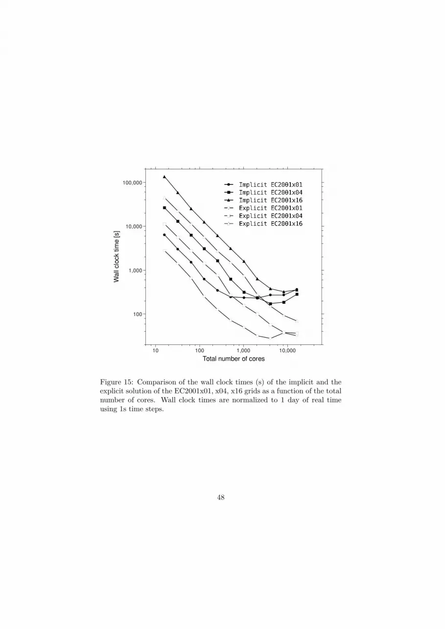
compare wall clock times as a function of the number of cores in Figure 15.

We note the linear or better than linear scaling caused by the cache effect.

The most pronounced manifestation of the cache effect occurs between 64

18

and 128 cores for the EC2001x01 grid; between 256 and 512 cores for the

EC2001x04 grid; and between 1,024 and 2,048 cores for the EC2001x16

grid. Ultimately all solutions lose strong scaling. However weak scaling is

evident in that the more finite element nodes a grid has, the longer it main-

tains its scaling. Furthermore, the explicit solutions maintain their scaling

much longer than the implicit solutions, and the performance improvement

as compared to the implicit solution becomes larger as the solutions’ scal-

ablity start to tail off. The implicit solution loses ideal scaling before 512

cores on the EC2001x01 grid, before 2,048 cores on the x04 grid, and be-

fore 8,192 cores on the x16 grid. After that, the wall clock times on all

grids increase to similar times, which is the effect of the increasing global

Allreduce communication times, the effect of local communications, as well

as the increasing numbers of overlapping finite element nodes. The explicit

solution loses scalability before 4,096 cores on the EC2001x01 grid, before

8,192 cores on x04 grid, and before 16,384 cores on x16 grid. The saturation

of wall clock time occurs at higher number of cores due to the increase in

the total number of finite element nodes originating from the overlapping

sub-domains as well as local communication time.

Figure 16 shows that all EC2001 grids behave similarly for the implicit

and explicit solutions when wall clock time is measured using the number

of finite element nodes per core. We again note that the explicit solution

is about twice as fast as the implicit solution, that all solutions have a well

defined cache boost, and that the explicit solution scales much longer than

the implicit solution. Figure 17 plots the parallel speed up as a function

of the number of finite element nodes per core. Both Figure 16 and Figure

17 suggest that for the EC2001 computations, the cache boost occurs at

19

about 2000 finite element nodes per core, reflecting that a boost occurs

somewhere between 4000 and 2000 finite element nodes per core. The op-

timal cache boost for the SL15 grids occured at approximately double that

number of finite element nodes per core, although the discrete doubling

increments make the exact boost points difficult to determine. In addition,

the scalability is sustained longer for the EC2001 computations than for

the SL15 computations. The reduction in scalability occurs below 1000

finite element nodes per core and is caused by a slow down in the scal-

ing of the local communication time as well as the increase in the relative

number of overlapping sub-domain finite element nodes. Figure 18 shows

this ratio and indicates the importance of the number of additional over-

lapping finite element nodes as the number of finite element nodes per core

decreases below 1,000. We also note that the EC2001 computations are

about twice faster than the SL15 computations on a wall clock time per

finite element node per core basis. The shift in the optimal cache boost,

the difference in simulation times, and the delayed reduction in scalability

reflect the fact that the SL15 computations include wetting and drying,

have much smaller finite elements, and include internal barrier boundaries.

This implies stronger nonlinear terms, resetting matrices, and more itera-

tions for the Conjugate Gradient matrix solver (for the implicit solution).

In addition, the wetting and drying algorithm and the internal barrier logic

require substantial computing time.

3.3 Comparison of results

In order to evaluate the time stepping accuracy, spatial accuracy, as well

as the difference between the implicit and explicit solution, we examine

20

the differences between the various solutions for a simulation of the storm

surge that developed during Hurricane Katrina [21][22].

First, in order to check the stability and accuracy of the time discretiza-

tions, we show a comparison of the water surface elevations near the peak

of the storm surge using different time step sizes for the SL15x01 grid. Fig-

ure 19 shows the distribution of water surface elevation and forcing wind

velocity vectors as the storm is developing the peak storm surge on the

SL15x01 grid for the implicit solution. Figure 20 shows the difference in

water surface elevation using an implicit solution with 1s and 0.5s time

steps, and Figure 21 shows the difference in elevation using an explicit so-

lution with 1s and 0.5s time steps. In these figures, there are no significant

differences in the numerical solutions and we can conclude that the selected

time steps are stable and accurate.

Next, we show a comparison of water surface elevations on grids with

different spatial resolutions. Figure 22 shows the difference in water eleva-

tion between the SL15x01 grid and SL15x04 grid for the implicit solution,

and Figure 23 shows this difference for the explicit solution. We used a

0.5s time step for both the SL15x01 grid and the SL15x04 grid. We note

that in the regions marked I in Figure 22,23 there are differences in the lim-

ited blue areas where the SL15x04 grid solution is larger than the SL15x01

grid solution. These areas have very shallow flow depths and have recently

been subject to the wetting and drying moving boundary. The wetting

and drying process converges as element size reduces and is therefore bet-

ter represented by the finer SL15x04 grid. Thus the SL15x01 grid needs a

higher density of elements around these areas. There is also a very limited

underprediction in the SL15x01 grid in region II, where overtopping weir

21

flow, computed using internal barrier boundary conditions, is greater in

the finer SL15x04 grid. Again the finer grid solution improves the solution.

Region III is at the interface of wind blowing water away from a levee and

gradient driven high water pushing its way towards the same levee. This

also represents a wet and dry interface which is again better represented

by the higher resolution grid.

Finally, we note that the spatial errors between the lower and higher

resolution SL15x01 and SL15x04 grids are essentially identical for implicit

and explicit solutions. A comparison between the implicit and explicit so-

lutions reflects this and we can not see significant differences between these

solutions with the exception of small regions near wet and dry interfaces,

as shown in Figure 24.

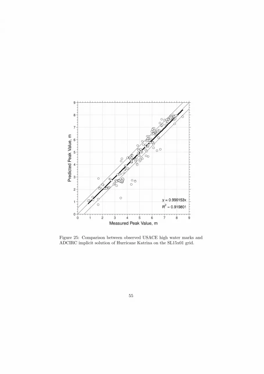
3.4 Model Validation

The SL15 model has been extensively validated against available tide, river

flow - stage, and hurricane Katrina and Rita high water mark (HWM) and

hydrograph data [21][22]. The hurricane hindcasts were forced with tides

on the Atlantic open ocean boundary, tidal potential functions that are de-

rived from solar and lunar gravitational forces, riverine flows, atmospheric

pressure, wind fields, and wind wave forces. The wind wave forcing is com-

puted through two way couplings to nested wave models and is especially

important in wave transformation zones. The SL15x01 grid applied in this

paper is an incremental refinement of the earlier SL15 model and has been

revalidated by simulating Hurricane Katrina using optimized data assimi-

lated wind fields [21]. Figures 25 and 26 compare the computed high water

during Hurricane Katrina to data collected by the U.S. Army Corps of

22

Engineers as well as by URS Corporation for the Federal Emergency Man-

agement Agency (FEMA) [28] [29]. The collected HWM’s are distributed

throughout coastal and inland southeastern Louisiana and Mississippi. The

figures indicate that there is essentially no bias (with best fit slopes of 0.99

and 1.02) and that there is a close fit between the computed and measured

data (with correlation coefficients squared equal to 0.92 and 0.94 respec-

tively).

3.5 File writing performance

In order to measure the performance of the dedicated writer cores, the

Hurricane Katrina storm surge simulation [21][22] was benchmarked with

the various writing options described in section 2.4. The wall clock times

were measured for a three hour real time simulation on the SL15x04 grid

with four output files (water surface elevation, the two components of the

velocity vector, the two components of the wind forcing vector, and atmo-

spheric pressure). Each output file was written to every fifteen minutes of

real time simulation (every 1,800 time steps) for all finite element nodes

on the global grid. Table 5 shows the wall clock times of the implicit and

explicit solution using 1,024 cores and 8,192 cores with no output, standard

output, with 1 dedicated writer core, 2 dedicated writer cores, 4 dedicated

writer cores, and 8 dedicated writer cores organized in 2 sequential batches.

In this table, the number inside of the parentheses shows the communica-

tion time used in writing the four output files, specifically the time required

for the compute cores to send the result data to the writer cores.

Figure 27 shows the wall clock times for the implicit solution. The stan-

dard output option, which uses one compute core as the data output col-

23

lector and writer, almost doubles the wall clock time due to disk array

latency. In this figure, the significant improvement achieved using the ded-

icated writer core algorithm is seen compared with the standard output

option. We note that the actual required writing time of the implicit solu-

tion with 1,024 cores using either 1, 2, 4, and 8 writer cores is less than the

computation time for any given output time interval. For the 8,192 core

case the actual required writing time to the four output files exceeds the

computation wall clock time for the output interval as the parallel scaling

has dramatically reduced (by a factor of 3.86) the computation wall clock

time. Therefore more dedicated writer cores are needed; in this case, two

suffices.

The explicit solution case shown in Figure 28 needs even more dedicated

writer cores for effective file output. For the 1,024 core case, the total run

time almost triples when the standard output option is used. We note that

the required total writing time is the same as for the implicit 1,024 core

case (approximately 1,085 seconds), but that the relative proportion of the

total run spent writing is larger. The use of one writer core is therefore

insufficient since the computation time between output intervals is smaller

than the total required writing time. Therefore at least two writer cores are

required. As can be seen in Figure 28 and Table 5, distributing the writing

process on two or more dedicated writer cores dramatically improves overall

performance. The explicit solution with 8,192 total cores exhibits the most

dramatic slow down when the standard output option is used, by more than

a factor of 12. It is clear that the scalable performance of this simulation is

destroyed by the file writing process. The 8,192 core explicit computation

time is in fact 7.3 times faster than the 1,024 core computation time while

24

the total required file output time is still about 1050 seconds for both

simulations. As noted in Figure 28 and Table 5, we now require 8 writer

cores organized in two sequential batches, which are simultaneously writing

2 sets of output files, to achieve improvements in the total wall clock time.

We note that the best total time with the 2 sequential batches of 4 writer

cores still exceeds the total simulation time without any writing. This is

due to the fact that the output data send time from the compute cores to

the writer cores (which varies between about 60 seconds and 112 seconds)

is asynchronous and is performed by the compute cores which can not be

computing while performing this operation as was illustrated in Figure 4.

Furthermore we note from Table 5 that the data send time does not scale,

either with the number of compute cores, or the number of writer cores.

The ideal time then is the no output time plus the data send time. This

is almost achieved, as seen in Table 5, although there is a discrepancy

between the best total time and the ideal time which varies between 5

seconds (for the 8,192 core, explicit case) and 97 seconds (for the 8,192

core, implicit case). This is likely related to data send time syncronization

which can be related to the variable data load that must be transmitted

and the congestion of network traffic.

4 CONCLUSIONS

The scalability of the continuous Galerkin implementation of the ADCIRC

unstructured grid shallow water equation model was measured for various

forcing function scenarios and on different resolution grids. Both implicit

and explicit implementations were examined. The implicit code shows

25

strong scaling on the TACC Ranger machine with up to about 2,000 finite

element nodes per core. The code also exhibits weak scaling with scalability

being sustained as long as the problem size is increased and at least 2,000

finite element nodes per core are used. The explicit solution is at least

twice as fast as the implicit solution on a per finite element node basis and

exhibits better and longer scalability since this solution does not require

the global communication that limits the scalability of the implicit solu-

tion. Ultimately as the number of finite element nodes per core decrease, all

solutions exhibit a deterioration in scalability due to local communication

times as well as a significant increase in the number of additional overlap-

ping finite element nodes at the subdomain interfaces. Finally, both the

implicit and explicit solutions experience a substantial cache boost when

between 2,000 and 4,000 finite element nodes per core are specified.

It is apparent that the required large scalar and vector output files for

water levels, currents, wind speed and atmospheric pressure can destroy

scalability and dramatically increase wall clock times. A dedicated writer

core algorithm was proposed for effective output file writing in order to

improve the total performance of the simulation with large and/or frequent

output file access. The writer core algorithm can use sequential batches of

writer cores so that sets of output files at sequential times can be written

synchronously. The dedicated writer cores contributed to the dramatic

improvement in simulation times effectively almost regaining simulation

times with no output with the exception of the required global data transfer

time between the compute cores and the dedicated writer cores which does

not scale.

It appears that the explicit solutions are an excellent choice for improving

26

wall clock times and sustaining scalability for large grids when a large

number of processors are available. The explicit solution may also be an

attractive option when performing simulations on a system with relatively

slow communications links. Comparisons between the implicit and explicit

solutions indicate that the solutions are almost identical when time steps

are selected that are sufficiently small to ensure accuracy and stability.

It is also clear that wall clock times can be achieved that allow the

CG ADCIRC model to be used for forecasting hurricane storm surge. A

9,314,706 finite element node grid with 1s time steps can complete a day

of real time simulation in between 200 and 400 wall clock seconds for the

computation plus approximately 400s of output communication time using

16,384 cores and the sequential batch dedicated writer core algorithm to

output water surface elevations, velocities, winds, and pressure every 30

min of real time. This suggests that a very high resolution simulation can

be achieved in less than 20 min of wall clock time per day of real time

simulation, well within forecasting time window requirements. Larger fi-

nite element grids can also be used due to the weak scaling characteristics

and the continued development of output file management which can help

further reduce the file output communication times.

Acknowledgements

This work was supported by awards from the National Science Founda-

tion (OCI-0749015, OCI-0746232, DMS-0620696, DMS-0620697 and DMS-

0620791) and the Office of Naval Research (N00014-06-1-0285). Compu-

tational resources were provided in part by awards from TACC and the

TeraGrid project (TGDMS080016N).

27

References

[1] Resio, D.T. and Westerink, J.J. (2008). Hurricanes and the Physics of

Surges. Physics Today, 61, 9, 33-38.

[2] Kolar, R.L., Westerink, J.J., Cantekin, M.E. and Blain, C.A. (1994).

Aspects of nonlinear simulations using shallow-water models based on

the wave continuity equation. Computers and Fluids, 23, 523-528.

[3] Luettich, R.A., Hu, S. and Westerink, J.J. (1994). Development of

the direct stress solution technique for three dimensional hydrody-

namic models using finite elements. International Journal for Numer-

ical Methods in Fluids, 19, 295-319.

[4] Grenier, R.R., Luettich, R.A. and Westerink, J.J. (1995). A compar-

ison of the nonlinear frictional characteristics of two-dimensional and

three-dimensional models of a shallow tidal embayment. Journal of

Geophysical Research, 100, C7, 13719-13735.

[5] Kolar, R.L., Gray, W.G. and Westerink, J.J. (1996). Boundary con-

ditions in shallow water models - an alternative implementation for

finite element codes. International Journal for Numerical Methods in

Fluids, 22, 603-618.

[6] Atkinson, J.H., Westerink, J.J. and Hervouet, J.M. (2004). Similarities

between the quasi-bubble and the generalized wave continuity equa-

tion solutions to the shallow water equations. International Journal

for Numerical Methods in Fluids, 45, 689-714.

[7] Atkinson, J.H., Westerink, J.J., Luettich, R.A. (2004). Two-

dimensional dispersion analyses of finite element approximations to the

28

shallow water equations. International Journal for Numerical Methods

in Fluids, 45, 715-749.

[8] Luettich, R.A. and Westerink, J.J. (2004). Formulation and Numerical

Implementation of the 2D/3D ADCIRC Finite Element Model Version

44.XX; http://adcirc.org/adcirc theory 2004 12 08.pdf

[9] Dawson, C., Westerink, J.J., Feyen, J.C. and Pothina, D. (2006). Con-

tinuous, discontinuous and coupled discontinuous-continuous Galerkin

finite element methods for the shallow water equations. International

Journal for Numerical Methods in Fluids, 52, 63-88.

[10] Kubatko, E.J., Westerink, J.J. and Dawson, C. (2006). hp discontin-

uous Galerkin methods for advection dominated problems in shallow

water flow. Computer Methods in Applied Mechanics and Engineering,

196, 437-451.

[11] Kubatko, E.J., Westerink, J.J. and Dawson, C. (2007). Semi-discrete

discontinuous Galerkin methods and stage exceeding order strong sta-

bility preserving Runge-Kutta time discretizations. Journal of Com-

putational Physics, 222, 832-848.

[12] Kubatko, E.J., Dawson, C. and Westerink, J.J. (2008). Time step

restrictions for Runge-Kutta discontinuous Galerkin methods on tri-

angular grids. Journal Computational Physics, 227, 9697-9710.

[13] Kubatko, E.J., Bunya, S., Dawson, C., Westerink, J.J. and Mirabito

C. (2009). A performance comparison of continuous and discontinuous

finite element shallow water models. Journal of Scientific Computing.

40, 315-339.

29

[14] Bunya, S., Kubatko, E.J., Westerink, J.J. and Dawson, C. (2009).

A wetting and drying treatment for the Runge-Kutta discontinuous

Galerkin solution to the shallow water equations. Computer Methods

in Applied Mechanics and Engineering, 198, 1548-1562.

[15] Kubatko, E.J., Bunya, S., Dawson, C. and Westerink, J.J. (2009).

Dynamic p-adaptive Runge-Kutta discontinuous Galerkin methods for

the shallow water equations. Computer Methods in Applied Mechanics

and Engineering, 198, 1766-1774.

[16] Westerink, J.J., Luettich, R.A. and J.C. Muccino, J.C. (1994). Mod-

eling tides in the western North Atlantic using unstructured graded

grids. Tellus, 46A, 178-199.

[17] Blain, C.A., Westerink, J.J. and Luettich, R.A. (1994). The influence

of domain size on the response characteristics of a hurricane storm

surge model. Journal of Geophysical Research, 99, C9, 18467-18479.

[18] Blain, C.A., Westerink, J.J. and Luettich, R.A. (1998). Grid conver-

gence studies for the prediction of hurricane storm surge. International

Journal for Numerical Methods in Fluids, 26, 369-401.

[19] Mukai, A., Westerink, J.J., Luettich, R.A. and Mark, D. (2002). East-

coast 2001: A tidal constituent database for the western North At-

lantic, Gulf of Mexico, and Caribbean Sea. Tec. Rep. ERDC/CHL

TR-02-24, U.S.Army Corps of Engineers, 25.

[20] Westerink, J.J., Luettich, R.A., Feyen, J.C., Atkinson, J.H., Dawson,

C., Roberts, H.J., Powell, M.D., Dunion, J.P., Kubatko, E.J., Pourta-

heri, H. (2008). A basin to channel scale unstructured grid hurricane

30

storm surge model applied to Southern Louisiana. Monthly Weather

Review, 136, 3, 833-864.

[21] Bunya, S., Dietrich, J.C., Westerink, J.J., Ebersole, B.A., Smith, J.M.,

Atkinson, J.H., Jensen, R., Resio, D.T., Luettich, R.A., Dawson, C.,

Cardone, V.J., Cox, A.T., Powell, M.D., Westerink, H.J., Roberts,

H.J. (2009). A high resolution coupled riverine flow tide, wind, wind

wave and storm surge model for Southern Louisiana and Mississippi:

part I - model development and validation. Monthly Weather Review,

DOI: 10.1175/2009MWR2907.1, in press.

[22] Dietrich, J.C., Bunya, S., Westerink, J.J., Ebersole, B.A., Smith, J.M.,

Atkinson, J.H., Jensen, R., Resio, D.T., Luettich, R.A., Dawson, C.,

Cardone, V.J., Cox, A.T., Powell, M.D., Westerink, H.J., Roberts,

H.J. (2009). A high resolution coupled riverine flow tide, wind, wind

wave and storm surge model for Southern Louisiana and Mississippi:

part II - synoptic description and analyses of hurricane Katrina and

Rita. Monthly Weather Review, DOI: 10.1175/2009MWR2906.1, in

press.

[23] http://www.tacc.utexas.edu/

[24] Kincaid, D.R., Respess, J.R., Young, D.M. and Grimes, R.G. (1982).

ITPACK 2C: A Fortran package for solving large sparse linear sys-

tems by adaptive accelerated iterative methods, ACM Transactions

on Mathematical Software, 8, No.3.

31

[25] Karypis, G. and Kumar, V. (1998). Multilevel k-way partitioning

scheme for irregular graphs. Journal of Parallel and Distributed Com-

puting. 48, No.1. 96-129.

[26] http://www.erdc.hpc.mil/systemNews/Cray XT3/home

[27] http://www.erdc.hpc.mil/systemNews/Cray XT4/home

[28] URS, (2006). Final coastal and riverine high-water marks collection

for Hurricane Katrina in Louisiana. FEMA-1603-DR-LA, Task Orders

412 and 419, Federal Emergency Management Agency, Washington

DC, 76pp.

[29] Ebersole, B.A., Westerink, J.J., Resio, D.T., and Dean, R.G. (2007).

Performance Evaluation of the New Orleans and Southeast Louisiana

Hurricane Protection System, Volume IV - The Storm. Final Report of

the Interagency Performance Evaluation Task Force, U.S. Army Corps

of Engineers, Washington, D.C., 263 pp.

32

Table 1: Specifications of TACC Ranger compute nodes

Sun Blade x6420 CPU 4 Quadcore AMD Opteron 8356

Memory 16×2GB DDR2-667 ECC-reg

AMD Opteron 8356 Frequency 2.3 GHz

Architecture AMD K10 (Barcelona)

L1-Cache 64+64KB per core

L2-Cache 512KB per core

L3-Cache 2048KB on die shared

Table 2: Finite element grids

Grid name Nnode Nelem he Wet/Dry Internal Barrier

SL15x01 2,351,832 4,611,048 30 m yes yes

SL15x04 9,314,706 18,444,184 15 m yes yes

EC2001x01 254,565 492,179 200 m no no

EC2001x04 1,001,418 1,968,716 100 m no no

EC2001x16 3,971,661 7,874,864 50 m no no

*Nnode: total number of nodes, Nelem: total number of elements, he: minimumelement size

33

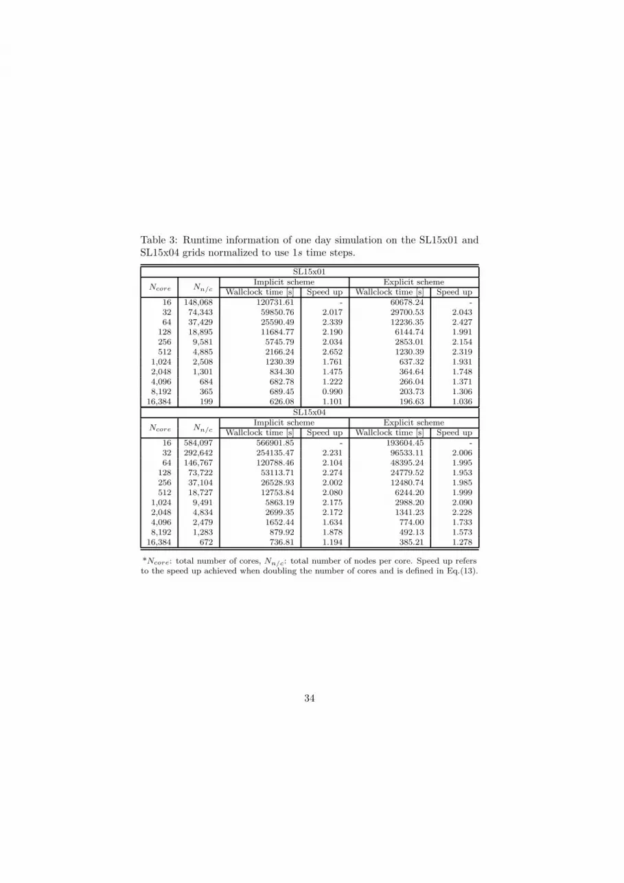
Table 3: Runtime information of one day simulation on the SL15x01 andSL15x04 grids normalized to use 1s time steps.

SL15x01

Ncore Nn/cImplicit scheme Explicit scheme

Wallclock time [s] Speed up Wallclock time [s] Speed up16 148,068 120731.61 - 60678.24 -32 74,343 59850.76 2.017 29700.53 2.04364 37,429 25590.49 2.339 12236.35 2.427

128 18,895 11684.77 2.190 6144.74 1.991256 9,581 5745.79 2.034 2853.01 2.154512 4,885 2166.24 2.652 1230.39 2.319

1,024 2,508 1230.39 1.761 637.32 1.9312,048 1,301 834.30 1.475 364.64 1.7484,096 684 682.78 1.222 266.04 1.3718,192 365 689.45 0.990 203.73 1.306

16,384 199 626.08 1.101 196.63 1.036

SL15x04



128 73,722 53113.71 2.274 24779.52 1.953256 37,104 26528.93 2.002 12480.74 1.985512 18,727 12753.84 2.080 6244.20 1.999

1,024 9,491 5863.19 2.175 2988.20 2.0902,048 4,834 2699.35 2.172 1341.23 2.2284,096 2,479 1652.44 1.634 774.00 1.7338,192 1,283 879.92 1.878 492.13 1.573

16,384 672 736.81 1.194 385.21 1.278

*Ncore: total number of cores, Nn/c: total number of nodes per core. Speed up refersto the speed up achieved when doubling the number of cores and is defined in Eq.(13).

34

Table 4: Runtime information of one day simulation on the EC2001x01,x04 and x16 grids normalized to use 1s time steps.

EC2001x01



128 2,107 625.45 2.428 251.22 2.637256 1,088 344.49 1.816 127.25 1.974512 567 245.86 1.401 72.33 1.759

1,024 302 234.96 1.046 49.91 1.4492,048 165 230.44 1.020 31.66 1.5774,096 92 270.93 0.851 27.71 1.1428,192 54 274.43 0.987 37.25 0.744

16,384 34 363.68 0.755 32.23 1.156

EC2001x04



128 8,059 3081.70 2.059 1416.87 1.955256 4,094 1635.11 1.885 770.18 1.840512 2,094 628.21 2.603 271.07 2.841

1,024 1,083 316.92 1.982 156.66 1.7302,048 566 236.33 1.341 101.73 1.5404,096 302 170.90 1.383 56.73 1.7938,192 165 185.71 0.920 38.03 1.491

16,384 93 282.04 0.658 36.82 1.033

EC2001x16



128 31,486 12520.63 2.015 5683.99 1.986256 15,873 6149.89 2.036 2760.32 2.059512 8,035 3125.73 1.968 1506.56 1.832

1,024 4,088 1593.64 1.961 754.09 1.9982,048 2,094 637.40 2.500 282.16 2.6734,096 1,084 380.80 1.674 150.97 1.8698,192 568 323.35 1.178 94.14 1.604

16,384 303 356.81 0.906 70.03 1.344

*Ncore: total number of cores, Nn/c: total number of nodes per core. Speed up refersto the speed up achieved when doubling the number of cores and is defined in Eq.(13).

35

Table 5: Wall clock times of three hour hurricane simulation with fouroutput files written every 15 min of simulation time and communication(send/receive) time used for writing (in parenthesis).

no output standard 1 wcore 2 wcore 4 wcore 8 wcore ideal

Implicit 1506.27 2590.86 1583.30 1611.09 1598.07 1612.17 15731,024 (63.19) (63.91) (66.39) (66.98)

Implicit 390.18 1467.59 977.18 549.76 504.42 576.17 4818,192 (89.24) (88.56) (90.75) (88.50)

Explicit 679.93 1767.81 1033.56 837.01 869.16 865.71 7921,024 (95.98) (94.38) (102.88) (112.17)

Explicit 92.86 1134.85 974.49 536.57 356.83 186.47 1818,192 (85.24) (78.22) (81.62) (88.50)

36

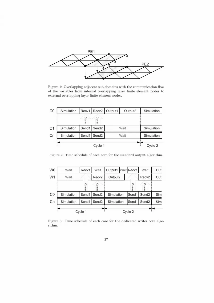
Figure 1: Overlapping adjacent sub-domains with the communication flowof the variables from internal overlapping layer finite element nodes toexternal overlapping layer finite element nodes.

Figure 2: Time schedule of each core for the standard output algorithm.

Figure 3: Time schedule of each core for the dedicated writer core algo-rithm.

37

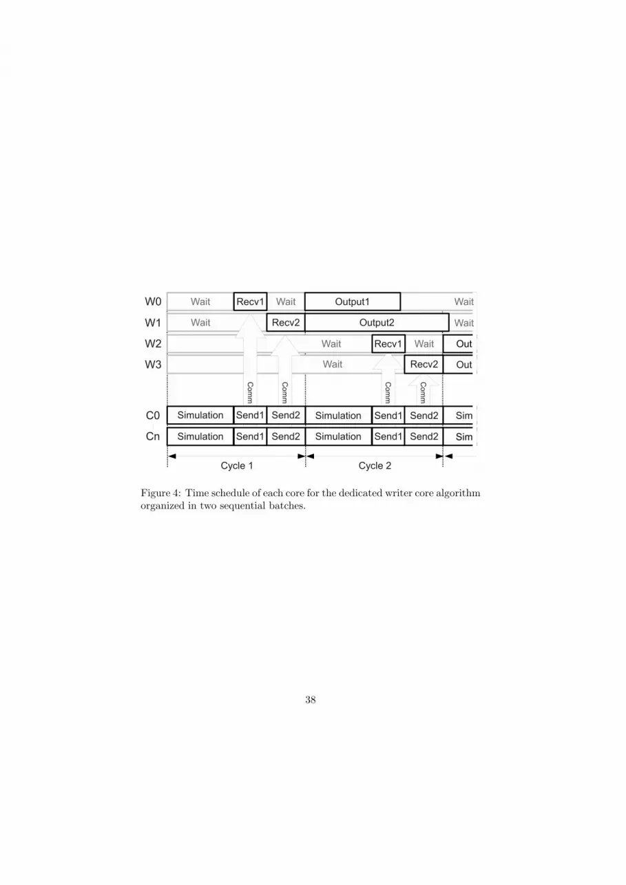
Figure 4: Time schedule of each core for the dedicated writer core algorithmorganized in two sequential batches.

38

Figure 5: Flow chart of the simulation.

39

Figure 6: SL15x01 grid colored by finite element size and the borders of1,024 subdomains.

40

Figure 7: EC2001x01 grid colored by finite element size and the borders of1,024 subdomains.

x01 x04 x16

Figure 8: Refinement of grids.

41

Wall clock tim

e [s]

100

1,000

10,000

100,000

1,000,0001,000,000

Total number of cores

10 100 1,000 10,000

Figure 9: Comparison of the wall clock times (s) of the implicit and theexplicit solution on the SL15x01, x04 grids as a function of the total numberof cores. Wall clock times are normalized to 1 day of real time using 1stime steps.

42

Wall clock tim

e [s]

100

1,000

10,000

100,000

1,000,0001,000,000

Total number of finite element nodes per core

100 1,000 10,000 100,000 1,000,0001,000,000

Figure 10: Comparison of the wall clock times of the implicit and theexplicit solution on the SL15x01, x04 grids as a function of the total numberof finite element nodes per core. Wall clock times are normalized to 1 dayof real time using 1s time steps.

43

Para

llel speed up

0.5

1.0

1.5

2.0

2.5

3.0

3.5


100 1,000 10,000 100,000 1,000,0001,000,000

Figure 11: Parallel speed up resulting from core doubling for implicit andexplicit solutions of the SL15x01, x04 grids as a function of the total numberof finite element nodes per core.

44

Wall clock tim

e [s]

100

1,000

10,000

100,000


100 1,000 10,000

Figure 12: Component computational times of the implicit solution of theSL15x04 grid.

45

Wall clock tim

e [s]

100

1,000

10,000

100,000


100 1,000 10,000

Figure 13: Component computational times of the explicit solution of theSL15x04 grid.

46

Ratio of the total number nodes of sub-d

omains

1.00

1.20

1.40


100 1,000 10,000 100,000 1,000,0001,000,000

Figure 14: The ratio of the sum of the total number of finite element nodeson all sub-domains to the original number of finite element nodes in theglobal grid for the SL15 grids as a function of the total number of finiteelement nodes per core.

47

Wall clock tim

e [s]

100

1,000

10,000

100,000


10 100 1,000 10,000

Figure 15: Comparison of the wall clock times (s) of the implicit and theexplicit solution of the EC2001x01, x04, x16 grids as a function of the totalnumber of cores. Wall clock times are normalized to 1 day of real timeusing 1s time steps.

48

Wall clock tim

e [s]

100

1,000

10,000

100,000


10 100 1,000 10,000 100,000 1,000,0001,000,000

Figure 16: Comparison of the wall clock times of the implicit and theexplicit solution on the EC2001x01, x04, x16 grids as a function of the totalnumber of finite element nodes per core. Wall clock times are normalizedto 1 day of real time using 1s time steps.

49

Para

llel speed up

0.5

1.0

1.5

2.0

2.5

3.0

3.5


10 100 1,000 10,000 100,000 1,000,0001,000,000

Figure 17: Parallel speed up resulting from core doubling for implicit andexplicit solutions of the EC2001x01, x04, x16 grids as a function of thetotal number of finite element nodes per core.

50

Ratio of the total number nodes of sub-d

omains

1.00

1.50

2.00

2.50


10 100 1,000 10,000 100,000 1,000,0001,000,000

Figure 18: The ratio of the sum of the total number of finite element nodeson all sub-domains to the original number of finite element nodes in theglobal grid for the EC2001 grids as a function of the total number of finiteelement nodes per core.

51

Figure 19: Water surface elevation (m) and wind velocity vectors (m/s)near the peak of the storm surge.

Figure 20: Difference in water surface elevations (m) between 1.0s and 0.5stime step implicit solutions of the SL15x01 grid.

52

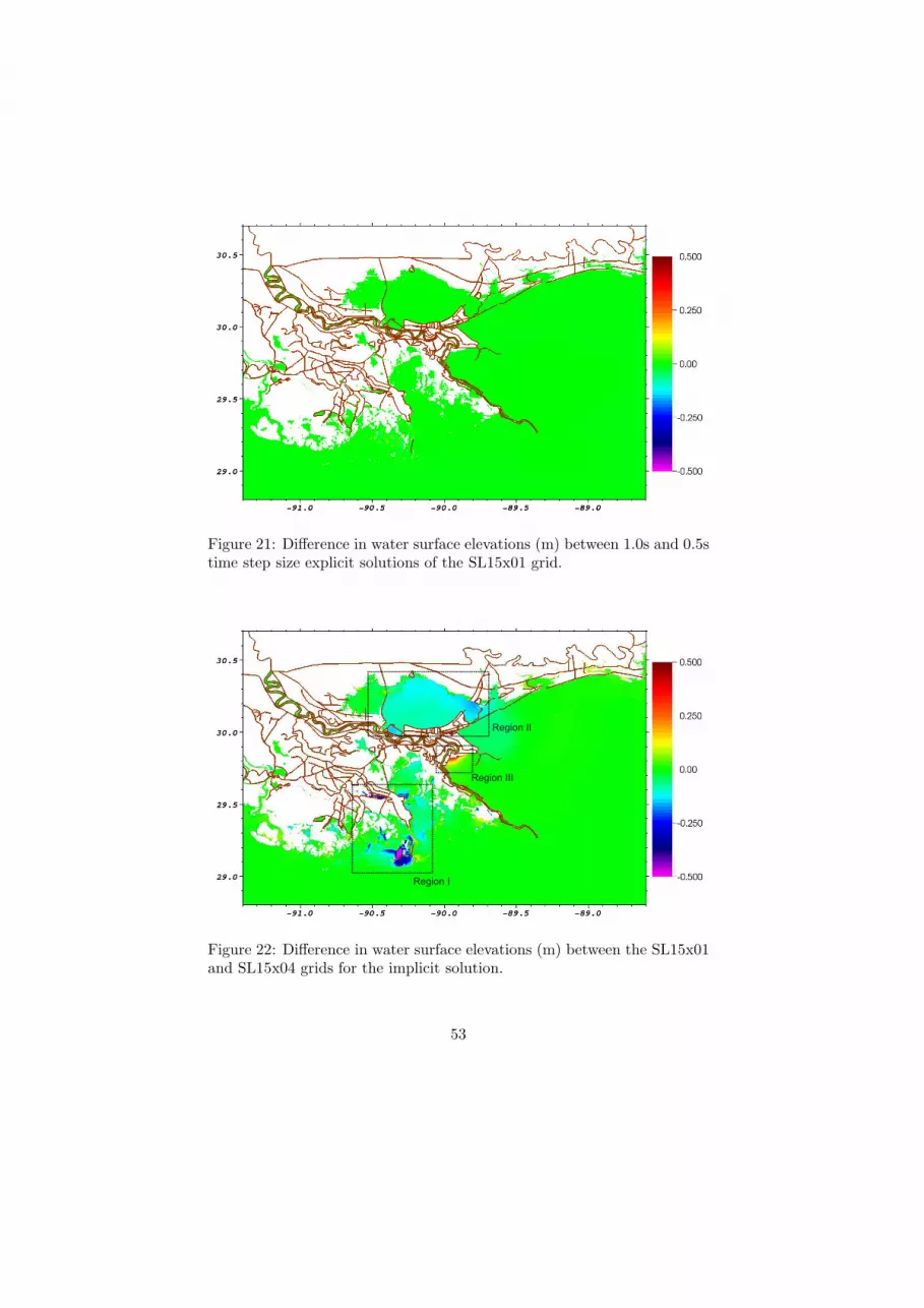
Figure 21: Difference in water surface elevations (m) between 1.0s and 0.5stime step size explicit solutions of the SL15x01 grid.

Figure 22: Difference in water surface elevations (m) between the SL15x01and SL15x04 grids for the implicit solution.

53

Figure 23: Difference in water surface elevations (m) between the SL15x01and SL15x04 grid for the explicit solution.

Figure 24: Difference in water surface elevations (m) between the implicitsolution and explicit solution of the SL15x01 grid.

54

Pre

dicted P

eak V

alue, m

0

1

2

3

4

5

6

7

8

9

Measured Peak Value, m

0 1 2 3 4 5 6 7 8 9

Figure 25: Comparison between observed USACE high water marks andADCIRC implicit solution of Hurricane Katrina on the SL15x01 grid.

55

Pre

dicted P

eak V

alue, m

0

1

2

3

4

5

6

7

8

9

Measured Peak Value, m

0 1 2 3 4 5 6 7 8 9

Figure 26: Comparison between observed URS high water marks and AD-CIRC implicit solution of Hurricane Katrina on the SL15x01 grid.

56

Wall clock tim

e [s]

0

500

1,000

1,500

2,000

2,500

3,000

1,024 cores

Wall clock tim

e [s]

0

500

1,000

1,500

2,000

2,500

3,000

8,192 cores

Figure 27: Performance of writing algorithms for the implicit solution ofthe SL15x04 grid; comparison of no output, standard output, with 1 dedi-cated writer core, 2 dedicated writer cores, 4 dedicated writer cores, and 8dedicated writer cores organized in 2 batches.

57

Wall clock tim

e [s]

0

500

1,000

1,500

2,000

2,500

3,000

1,024 cores

Wall clock tim

e [s]

0

500

1,000

1,500

2,000

2,500

3,000

8,192 cores

Figure 28: Performance of writing algorithms for the explicit solution ofthe SL15x04 grid; comparison of no output, standard output, with 1 dedi-cated writer core, 2 dedicated writer cores, 4 dedicated writer cores, and 8dedicated writer cores organized in 2 batches.

58

Scalability of an Unstructured Grid Continuous Galerkin Based Hurricane Storm Surge Model

Documents