CHAPTER FOURTEEN SIMPLE LINEAR REGRESSION MULTIPLE CHOICE QUESTIONS In the following multiple choice questions, circle the correct answer. 1. The standard error is the a. t-statistic squared b. square root of SSE c. square root of SST d. square root of MSE Answer: d 2. If MSE is known, you can compute the a. r square b. coefficient of determination c. standard error d. all of these alternatives are correct Answer: c 3. In regression analysis, which of the following is not a required assumption about the error term ? a. The expected value of the error term is one. b. The variance of the error term is the same for all values of X. c. The values of the error term are independent. d. The error term is normally distributed. Answer: a 4. A regression analysis between sales (Y in $1000) and advertising (X in dollars) resulted in the following equation = 30,000 + 4 X 1

Welcome message from author
This document is posted to help you gain knowledge. Please leave a comment to let me know what you think about it! Share it to your friends and learn new things together.
Transcript
CHAPTER FOURTEENSIMPLE LINEAR REGRESSION
MULTIPLE CHOICE QUESTIONS
In the following multiple choice questions, circle the correct answer.
1. The standard error is the a. t-statistic squaredb. square root of SSEc. square root of SSTd. square root of MSEAnswer: d
2. If MSE is known, you can compute thea. r squareb. coefficient of determinationc. standard errord. all of these alternatives are correctAnswer: c
3. In regression analysis, which of the following is not a required assumption about the error term ?a. The expected value of the error term is one.b. The variance of the error term is the same for all values of X.c. The values of the error term are independent.d. The error term is normally distributed.Answer: a
4. A regression analysis between sales (Y in $1000) and advertising (X in dollars) resulted in the following equation
= 30,000 + 4 X
The above equation implies that ana. increase of $4 in advertising is associated with an increase of $4,000 in salesb. increase of $1 in advertising is associated with an increase of $4 in salesc. increase of $1 in advertising is associated with an increase of $34,000 in salesd. increase of $1 in advertising is associated with an increase of $4,000 in salesAnswer: d
5. Regression analysis is a statistical procedure for developing a mathematical equation that describes howa. one independent and one or more dependent variables are related
1
2 Chapter Fourteen
b. several independent and several dependent variables are relatedc. one dependent and one or more independent variables are relatedd. None of these alternatives is correct.Answer: c
6. In a simple regression analysis (where Y is a dependent and X an independent variable), if the Y intercept is positive, thena. there is a positive correlation between X and Yb. if X is increased, Y must also increasec. if Y is increased, X must also increased. None of these alternatives is correct.Answer: d
7. In regression analysis, the variable that is being predicted is thea. dependent variableb. independent variablec. intervening variabled. is usually xAnswer: a
8. The equation that describes how the dependent variable (y) is related to the independent variable (x) is calleda. the correlation modelb. the regression modelc. correlation analysisd. None of these alternatives is correct.Answer: b
9. In regression analysis, the independent variable is a. used to predict other independent variablesb. used to predict the dependent variablec. called the intervening variabled. the variable that is being predictedAnswer: b
10. Larger values of r2 imply that the observations are more closely grouped about thea. average value of the independent variablesb. average value of the dependent variablec. least squares lined. originAnswer: c
11. In a regression model involving more than one independent variable, which of the following tests must be used in order to determine if the relationship between the dependent variable and the set of independent variables is significant?a. t test

Simple Linear Regression 3
b. F testc. Either a t test or a chi-square test can be used.d. chi-square testAnswer: b
12. In simple linear regression analysis, which of the following is not true?a. The F test and the t test yield the same results.b. The F test and the t test may or may not yield the same results.c. The relationship between X and Y is represented by means of a straight line.d. The value of F = t2.Answer: b
13. Correlation analysis is used to determinea. the equation of the regression lineb. the strength of the relationship between the dependent and the independent
variablesc. a specific value of the dependent variable for a given value of the independent
variabled. None of these alternatives is correct.Answer: b
14. In a regression and correlation analysis if r2 = 1, then a. SSE must also be equal to oneb. SSE must be equal to zeroc. SSE can be any positive valued. SSE must be negativeAnswer: b
15. In a regression and correlation analysis if r2 = 1, then a. SSE = SSTb. SSE = 1c. SSR = SSEd. SSR = SSTAnswer: d
16. In the case of a deterministic model, if a value for the independent variable is specified, then thea. exact value of the dependent variable can be computedb. value of the dependent variable can be computed if the same units are usedc. likelihood of the dependent variable can be computedd. None of these alternatives is correct.Answer: a
17. In a regression analysis if SSE = 200 and SSR = 300, then the coefficient of determination isa. 0.6667
4 Chapter Fourteen
b. 0.6000c. 0.4000d. 1.5000Answer: b
18. If the coefficient of determination is equal to 1, then the coefficient of correlationa. must also be equal to 1b. can be either -1 or +1c. can be any value between -1 to +1d. must be -1Answer: b
19. In a regression analysis, the variable that is being predicted a. must have the same units as the variable doing the predictingb. is the independent variablec. is the dependent variabled. usually is denoted by xAnswer: c
20. Regression analysis was applied between demand for a product (Y) and the price of the product (X), and the following estimated regression equation was obtained.
= 120 - 10 X
Based on the above estimated regression equation, if price is increased by 2 units, then demand is expected toa. increase by 120 unitsb. increase by 100 unitsc. increase by 20 unitsd. decease by 20 unitsAnswer: d
21. The coefficient of correlationa. is the square of the coefficient of determinationb. is the square root of the coefficient of determinationc. is the same as r-squared. can never be negativeAnswer: b
22. If the coefficient of determination is a positive value, then the regression equationa. must have a positive slopeb. must have a negative slopec. could have either a positive or a negative sloped. must have a positive y interceptAnswer: c

Simple Linear Regression 5
23. If the coefficient of correlation is 0.8, the percentage of variation in the dependent variable explained by the variation in the independent variable isa. 0.80%b. 80%c. 0.64%d. 64%Answer: d
24. In regression and correlation analysis, if SSE and SST are known, then with this information thea. coefficient of determination can be computedb. slope of the line can be computedc. Y intercept can be computedd. x intercept can be computedAnswer: a
25. In regression analysis, if the independent variable is measured in pounds, the dependent variablea. must also be in poundsb. must be in some unit of weightc. can not be in poundsd. can be any unitsAnswer: d
26. If there is a very weak correlation between two variables, then the coefficient of determination must bea. much larger than 1, if the correlation is positiveb. much smaller than 1, if the correlation is negativec. much larger than oned. None of these alternatives is correct.Answer: d
27. SSE can never bea. larger than SSTb. smaller than SSTc. equal to 1d. equal to zeroAnswer: a
28. If the coefficient of correlation is a positive value, then the slope of the regression linea. must also be positiveb. can be either negative or positivec. can be zerod. can not be zeroAnswer: a

6 Chapter Fourteen
29. If the coefficient of correlation is a negative value, then the coefficient of determinationa. must also be negativeb. must be zeroc. can be either negative or positived. must be positiveAnswer: d
30. It is possible for the coefficient of determination to bea. larger than 1b. less than onec. less than -1d. None of these alternatives is correct.Answer: b
31. If two variables, x and y, have a good linear relationship, thena. there may or may not be any causal relationship between x and yb. x causes y to happenc. y causes x to happend. None of these alternatives is correct.Answer: a
32. If the coefficient of determination is 0.81, the coefficient of correlationa. is 0.6561b. could be either + 0.9 or - 0.9c. must be positived. must be negativeAnswer: b
33. A least squares regression linea. may be used to predict a value of y if the corresponding x value is givenb. implies a cause-effect relationship between x and yc. can only be determined if a good linear relationship exists between x and yd. None of these alternatives is correct.Answer: a
34. If all the points of a scatter diagram lie on the least squares regression line, then the coefficient of determination for these variables based on this data isa. 0b. 1c. either 1 or -1, depending upon whether the relationship is positive or negatived. could be any value between -1 and 1Answer: b
35. If a data set has SSR = 400 and SSE = 100, then the coefficient of determination

Simple Linear Regression 7
isa. 0.10b. 0.25c. 0.40d. 0.80Answer: d
36. Compared to the confidence interval estimate for a particular value of y (in a linear regression model), the interval estimate for an average value of y will bea. narrowerb. widerc. the samed. None of these alternatives is correct.Answer: a
37. A regression analysis between sales (in $1000) and price (in dollars) resulted in the following equation
= 50,000 - 8X
The above equation implies that ana. increase of $1 in price is associated with a decrease of $8 in salesb. increase of $8 in price is associated with an increase of $8,000 in salesc. increase of $1 in price is associated with a decrease of $42,000 in salesd. increase of $1 in price is associated with a decrease of $8000 in salesAnswer: d
38. In a regression analysis if SST = 500 and SSE = 300, then the coefficient of determination isa. 0.20b. 1.67c. 0.60d. 0.40Answer: d
39. Regression analysis was applied between sales (in $1000) and advertising (in $100) and the following regression function was obtained.
= 500 + 4 X
Based on the above estimated regression line if advertising is $10,000, then the point estimate for sales (in dollars) isa. $900b. $900,000c. $40,500d. $505,000
8 Chapter Fourteen
Answer: b
40. The coefficient of correlationa. is the square of the coefficient of determinationb. is the square root of the coefficient of determinationc. is the same as r-squared. can never be negativeAnswer: b
41. If the coefficient of correlation is 0.4, the percentage of variation in the dependent variable explained by the variation in the independent variablea. is 40%b. is 16%.c. is 4%d. can be any positive valueAnswer: b
42. In regression analysis if the dependent variable is measured in dollars, the independent variablea. must also be in dollarsb. must be in some units of currencyc. can be any unitsd. can not be in dollarsAnswer: c
43. If there is a very weak correlation between two variables then the coefficient of correlation must bea. much larger than 1, if the correlation is positiveb. much smaller than 1, if the correlation is negativec. any value larger than 1d. None of these alternatives is correct.Answer: d
44. If the coefficient of correlation is a negative value, then the coefficient of determinationa. must also be negativeb. must be zeroc. can be either negative or positived. must be positiveAnswer: d
45. A regression analysis between demand (Y in 1000 units) and price (X in dollars) resulted in the following equation
= 9 - 3X

Simple Linear Regression 9
The above equation implies that if the price is increased by $1, the demand is expected toa. increase by 6 unitsb. decrease by 3 unitsc. decrease by 6,000 unitsd. decrease by 3,000 unitsAnswer: d
46. In a regression analysis if SST=4500 and SSE=1575, then the coefficient of determination isa. 0.35b. 0.65c. 2.85d. 0.45Answer: b
47. Regression analysis was applied between sales (in $10,000) and advertising (in $100) and the following regression function was obtained.
Y = 50 + 8 X
Based on the above estimated regression line if advertising is $1,000, then the point estimate for sales (in dollars) isa. $8,050b. $130c. $130,000d. $1,300,000Answer: d
48. If the coefficient of correlation is a positive value, thena. the intercept must also be positiveb. the coefficient of determination can be either negative or positive, depending
on the value of the slopec. the regression equation could have either a positive or a negative sloped. the slope of the line must be positiveAnswer: d
49. If the coefficient of determination is 0.9, the percentage of variation in the dependent variable explained by the variation in the independent variablea. is 0.90%b. is 90%.c. is 0.81%d. can be any positive valueAnswer: b
50. Regression analysis was applied between sales (Y in $1,000) and advertising (X
10 Chapter Fourteen
in $100), and the following estimated regression equation was obtained.
= 80 + 6.2 X
Based on the above estimated regression line, if advertising is $10,000, then the point estimate for sales (in dollars) isa. $62,080b. $142,000c. $700d. $700,000Answer: d
Exhibit 14-1The following information regarding a dependent variable (Y) and an independent variable (X) is provided.
Y X4 23 14 46 38 5
SSE = 6SST = 16
51. Refer to Exhibit 14-1. The least squares estimate of the Y intercept isa. 1b. 2c. 3d. 4Answer: b
52. Refer to Exhibit 14-1. The least squares estimate of the slope isa. 1b. 2c. 3d. 4Answer: a
53. Refer to Exhibit 14-1. The coefficient of determination isa. 0.7096b. - 0.7906c. 0.625d. 0.375Answer: c
Simple Linear Regression 11
54. Refer to Exhibit 14-1. The coefficient of correlation isa. 0.7096b. - 0.7906c. 0.625d. 0.375Answer: a
55. Refer to Exhibit 14-1. The MSE isa. 1b. 2c. 3d. 4Answer: b
Exhibit 14-2You are given the following information about y and x.
y xDependent Variable Independent Variable
5 14 23 32 41 5
56. Refer to Exhibit 14-2. The least squares estimate of b1 equalsa. 1b. -1c. 6d. 5Answer: b
57. Refer to Exhibit 14-2. The least squares estimate of b0 equalsa. 1b. -1c. 6d. 5Answer: c
58. Refer to Exhibit 14-2. The point estimate of y when x = 10 isa. -10b. 10c. -4d. 4Answer: c
12 Chapter Fourteen
59. Refer to Exhibit 14-2. The sample correlation coefficient equalsa. 0b. +1c. -1d. -0.5Answer: c
60. Refer to Exhibit 14-2. The coefficient of determination equalsa. 0b. -1c. +1d. -0.5Answer: c
Exhibit 14-3You are given the following information about y and x.
y xDependent Variable Independent Variable
12 43 67 26 4
61. Refer to Exhibit 14-3. The least squares estimate of b1 equalsa. 1b. -1c. -11d. 11Answer: b
62. Refer to Exhibit 14-3. The least squares estimate of b0 equalsa. 1b. -1c. -11d. 11Answer: d
63. Refer to Exhibit 14-3. The sample correlation coefficient equalsa. -0.4364b. 0.4364c. -0.1905d. 0.1905Answer: a

Simple Linear Regression 13
64. Refer to Exhibit 14-3. The coefficient of determination equalsa. -0.4364b. 0.4364c. -0.1905d. 0.1905Answer: d
Exhibit 14-4Regression analysis was applied between sales data (in $1,000s) and advertising data (in $100s) and the following information was obtained.
Ŷ= 12 + 1.8 x
n = 17SSR = 225SSE = 75Sb1 = 0.2683
65. Refer to Exhibit 14-4. Based on the above estimated regression equation, if advertising is $3,000, then the point estimate for sales (in dollars) is a. $66,000b. $5,412c. $66d. $17,400Answer: a
66. Refer to Exhibit 14-4. The F statistic computed from the above data isa. 3b. 45c. 48d. 50Answer: b
67. Refer to Exhibit 14-4. To perform an F test, the p-value isa. less than .01b. between .01 and .025c. between .025 and .05d. between .05 and 0.1Answer: d
68. Refer to Exhibit 14-4. The t statistic for testing the significance of the slope isa. 1.80b. 1.96c. 6.709d. 0.555Answer: c

14 Chapter Fourteen
69. Refer to Exhibit 14-4. The critical t value for testing the significance of the slope at 95% confidence isa. 1.753b. 2.131c. 1.746d. 2.120Answer: b
Exhibit 14-5The following information regarding a dependent variable (Y) and an independent variable (X) is provided.
Y X1 12 23 34 45 5
70. Refer to Exhibit 14-5. The least squares estimate of the Y intercept isa. 1b. 0c. -1d. 3Answer: b
71. Refer to Exhibit 14-5. The least squares estimate of the slope isa. 1b. -1c. 0d. 3Answer: a
72. Refer to Exhibit 14-5. The coefficient of correlation isa. 0b. -1c. 0.5d. 1Answer: d
73. Refer to Exhibit 14-5. The coefficient of determination isa. 0b. -1c. 0.5d. 1
Simple Linear Regression 15
Answer: d
74. Refer to Exhibit 14-5. The MSE isa. 0b. -1c. 1d. 0.5Answer: a
Exhibit 14-6For the following data the value of SSE = 0.4130.
y xDependent Variable Independent Variable
15 417 623 217 4
75. Refer to Exhibit 14-6. The slope of the regression equation isa. 18b. 24c. 0.707d. -1.5Answer: d
76. Refer to Exhibit 14-6. The y intercept isa. -1.5b. 24c. 0.50d. -0.707Answer: b
77. Refer to Exhibit 14-6. The total sum of squares (SST) equalsa. 36b. 18c. 9d. 1296Answer: a
78. Refer to Exhibit 14-6. The coefficient of determination (r2) equalsa. 0.7071b. -0.7071c. 0.5d. -0.5Answer: c

16 Chapter Fourteen
Exhibit 14-7You are given the following information about y and x.
y xDependent Variable Independent Variable
5 47 69 2
11 4
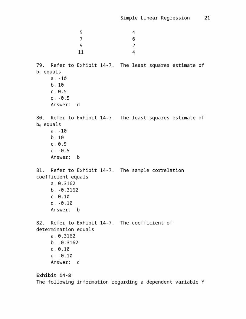
79. Refer to Exhibit 14-7. The least squares estimate of b1 equalsa. -10b. 10c. 0.5d. -0.5Answer: d
80. Refer to Exhibit 14-7. The least squares estimate of b0 equalsa. -10b. 10c. 0.5d. -0.5Answer: b
81. Refer to Exhibit 14-7. The sample correlation coefficient equalsa. 0.3162b. -0.3162c. 0.10d. -0.10Answer: b
82. Refer to Exhibit 14-7. The coefficient of determination equalsa. 0.3162b. -0.3162c. 0.10d. -0.10Answer: c
Exhibit 14-8The following information regarding a dependent variable Y and an independent variable X is provided
X = 90 = -156Y = 340 = 234n = 4 = 1974SSR = 104
Simple Linear Regression 17
83. Refer to Exhibit 14-8. The total sum of squares (SST) isa. -156b. 234c. 1870d. 1974Answer: d
84. Refer to Exhibit 14-8. The sum of squares due to error (SSE) isa. -156b. 234c. 1870d. 1974Answer: c
85. Refer to Exhibit 14-8. The mean square error (MSE) isa. 1870b. 13c. 1974d. 233.75Answer: d
86. Refer to Exhibit 14-8. The slope of the regression equation isa. -0.667b. 0.667c. 40d. -40Answer: a
87. Refer to Exhibit 14-8. The Y intercept isa. -0.667b. 0.667c. 40d. -40Answer: c
88. Refer to Exhibit 14-8. The coefficient of correlation isa. -0.2295b. 0.2295c. 0.0527d. -0.0572Answer: a
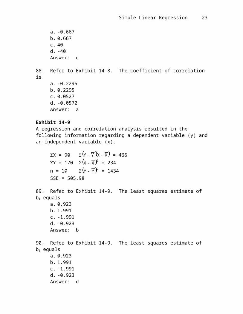
Exhibit 14-9A regression and correlation analysis resulted in the following information regarding a dependent variable (y) and an independent variable (x).
18 Chapter Fourteen
X = 90 = 466Y = 170 = 234n = 10 = 1434SSE = 505.98
89. Refer to Exhibit 14-9. The least squares estimate of b1 equalsa. 0.923b. 1.991c. -1.991d. -0.923Answer: b
90. Refer to Exhibit 14-9. The least squares estimate of b0 equalsa. 0.923b. 1.991c. -1.991d. -0.923Answer: d
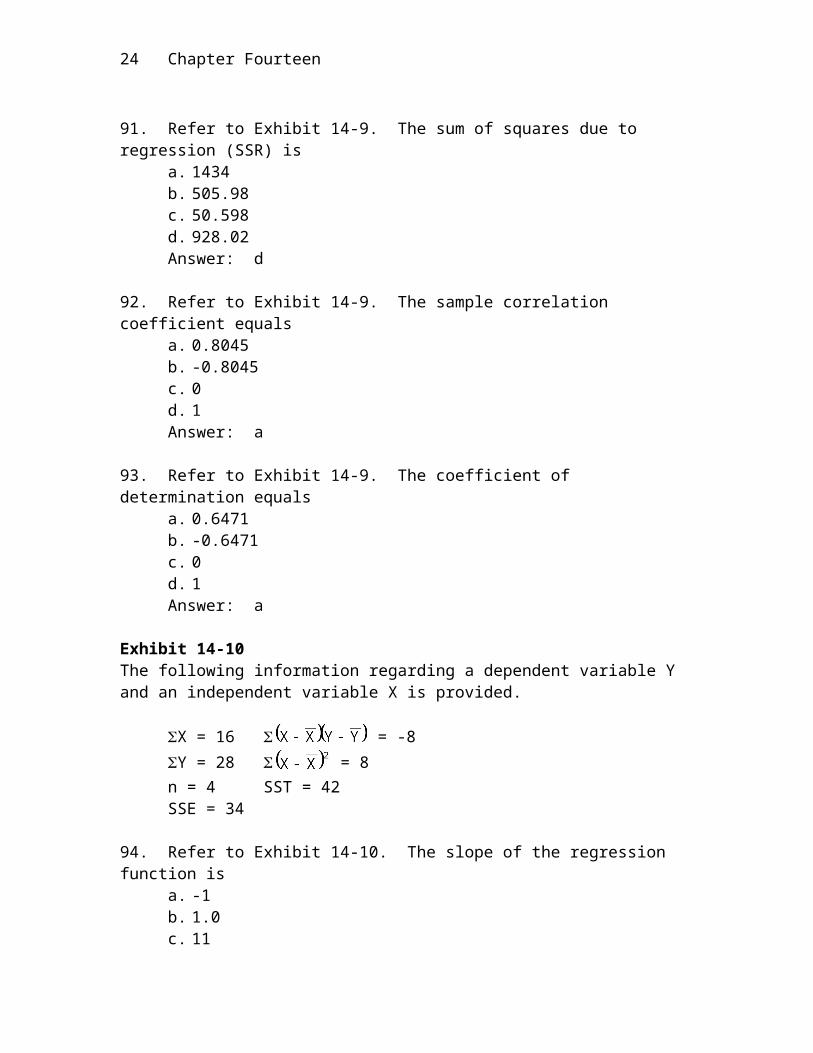
91. Refer to Exhibit 14-9. The sum of squares due to regression (SSR) isa. 1434b. 505.98c. 50.598d. 928.02Answer: d
92. Refer to Exhibit 14-9. The sample correlation coefficient equalsa. 0.8045b. -0.8045c. 0d. 1Answer: a
93. Refer to Exhibit 14-9. The coefficient of determination equalsa. 0.6471b. -0.6471c. 0d. 1Answer: a
Exhibit 14-10The following information regarding a dependent variable Y and an independent variable X is provided.
X = 16 = -8
Simple Linear Regression 19
Y = 28 = 8n = 4 SST = 42SSE = 34
94. Refer to Exhibit 14-10. The slope of the regression function isa. -1b. 1.0c. 11d. 0.0Answer: a
95. Refer to Exhibit 14-10. The Y intercept isa. -1b. 1.0c. 11d. 0.0Answer: c
96. Refer to Exhibit 14-10. The coefficient of determination isa. 0.1905b. -0.1905c. 0.4364d. -0.4364Answer: a
97. Refer to Exhibit 14-10. The coefficient of correlation isa. 0.1905b. -0.1905c. 0.4364d. -0.4364Answer: d
98. Refer to Exhibit 14-10. The MSE isa. 17b. 8c. 34d. 42Answer: a
99. Refer to Exhibit 14-10. The point estimate of Y when X = 3 isa. 11b. 14c. 8d. 0Answer: c
20 Chapter Fourteen
100. Refer to Exhibit 14-10. The point estimate of Y when X = -3 isa. 11b. 14c. 8d. 0Answer: b
Simple Linear Regression 21
PROBLEMS
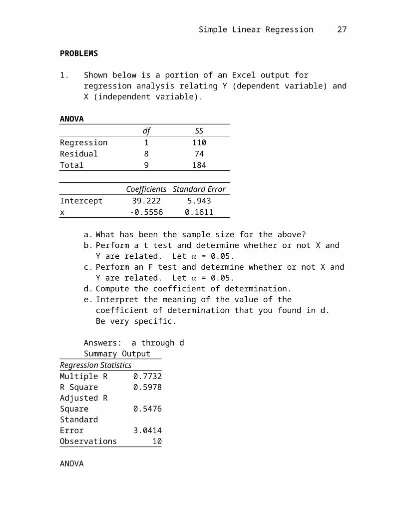
1. Shown below is a portion of an Excel output for regression analysis relating Y (dependent variable) and X (independent variable).
ANOVA df SS
Regression 1 110Residual 8 74Total 9 184
Coefficients Standard ErrorIntercept 39.222 5.943x -0.5556 0.1611
a. What has been the sample size for the above?b. Perform a t test and determine whether or not X and Y are related. Let =
0.05.c. Perform an F test and determine whether or not X and Y are related. Let =
0.05.d. Compute the coefficient of determination. e. Interpret the meaning of the value of the coefficient of determination that you
found in d. Be very specific.
Answers: a through dSummary Output
Regression StatisticsMultiple R 0.7732R Square 0.5978Adjusted R Square 0.5476Standard Error 3.0414Observations 10
ANOVA df SS MS F Significance F
Regression 1 110 110 11.892 0.009Residual 8 74 9.25Total 9 184
Coefficients Standard Error t Stat P-valueIntercept 39.222 5.942 6.600 0.000x -0.556 0.161 -3.448 0.009

22 Chapter Fourteen
e. 59.783% of the variability in Y is explained by the variability in X.
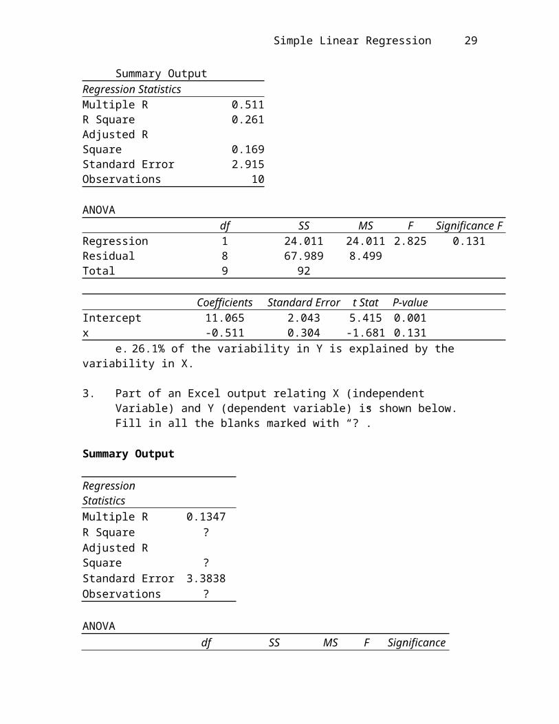
2. Shown below is a portion of a computer output for regression analysis relating Y (dependent variable) and X (independent variable).
ANOVA df SS
Regression 1 24.011Residual 8 67.989
Coefficients Standard ErrorIntercept 11.065 2.043x -0.511 0.304
a. What has been the sample size for the above?b. Perform a t test and determine whether or not X and Y are related. Let =
0.05.c. Perform an F test and determine whether or not X and Y are related. Let =
0.05.d. Compute the coefficient of determination. e. Interpret the meaning of the value of the coefficient of determination that you
found in d. Be very specific.
Answers: a through dSummary Output
Regression StatisticsMultiple R 0.511R Square 0.261Adjusted R Square 0.169Standard Error 2.915Observations 10
ANOVA df SS MS F Significance F
Regression 1 24.011 24.011 2.825 0.131Residual 8 67.989 8.499Total 9 92
Coefficients Standard Error t Stat P-valueIntercept 11.065 2.043 5.415 0.001x -0.511 0.304 -1.681 0.131
e. 26.1% of the variability in Y is explained by the variability in X.
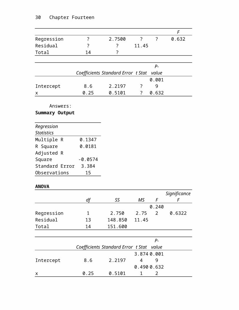
3. Part of an Excel output relating X (independent Variable) and Y (dependent vari-
Simple Linear Regression 23
able) is shown below. Fill in all the blanks marked with “?”.
Summary Output
Regression Statistics Multiple R 0.1347R Square ?Adjusted R Square ?Standard Error 3.3838Observations ?
ANOVA
df SS MS FSignificance
FRegression ? 2.7500 ? ? 0.632Residual ? ? 11.45Total 14 ?
Coefficients Standard Error t StatP-
value Intercept 8.6 2.2197 ? 0.0019x 0.25 0.5101 ? 0.632
Answers:Summary Output
Regression Statistics Multiple R 0.1347R Square 0.0181Adjusted R Square -0.0574Standard Error 3.384Observations 15
ANOVA
df SS MS FSignificance
FRegression 1 2.750 2.75 0.2402 0.6322Residual 13 148.850 11.45Total 14 151.600
Coefficients Standard Error t StatP-
value Intercept 8.6 2.2197 3.8744 0.0019
24 Chapter Fourteen
x 0.25 0.5101 0.4901 0.6322
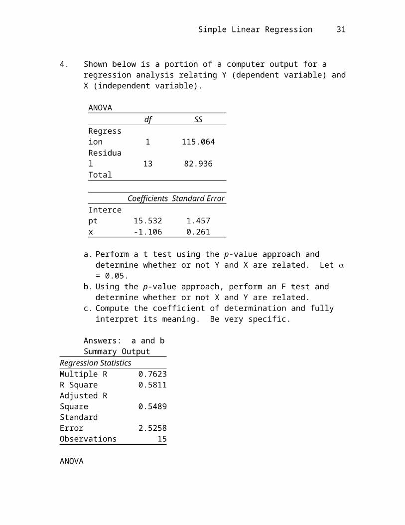
4. Shown below is a portion of a computer output for a regression analysis relating Y (dependent variable) and X (independent variable).
ANOVA df SS
Regression 1 115.064Residual 13 82.936Total
Coefficients Standard ErrorIntercept 15.532 1.457x -1.106 0.261
a. Perform a t test using the p-value approach and determine whether or not Y and X are related. Let = 0.05.
b. Using the p-value approach, perform an F test and determine whether or not X and Y are related.
c. Compute the coefficient of determination and fully interpret its meaning. Be very specific.
Answers: a and bSummary Output
Regression StatisticsMultiple R 0.7623R Square 0.5811Adjusted R Square 0.5489Standard Error 2.5258Observations 15
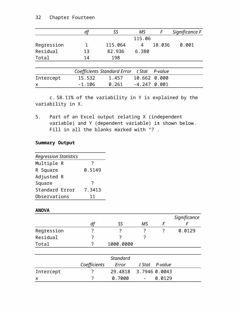
ANOVA df SS MS F Significance F
Regression 1 115.064 115.064 18.036 0.001Residual 13 82.936 6.380Total 14 198
Coefficients Standard Error t Stat P-valueIntercept 15.532 1.457 10.662 0.000x -1.106 0.261 -4.247 0.001
c. 58.11% of the variability in Y is explained by the variability in X.

Simple Linear Regression 25
5. Part of an Excel output relating X (independent variable) and Y (dependent variable) is shown below. Fill in all the blanks marked with “?”.
Summary Output
Regression Statistics Multiple R ?R Square 0.5149Adjusted R Square ?Standard Error 7.3413Observations 11
ANOVA
df SS MS FSignificance
FRegression ? ? ? ? 0.0129Residual ? ? ?Total ? 1000.0000
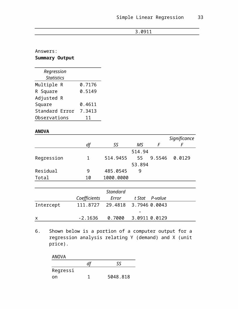
Coefficients Standard Error t Stat P-value Intercept ? 29.4818 3.7946 0.0043x ? 0.7000 -3.0911 0.0129
Answers:Summary Output
Regression Statistics Multiple R 0.7176R Square 0.5149Adjusted R Square 0.4611Standard Error 7.3413Observations 11
ANOVA
df SS MS FSignificance
FRegression 1 514.9455 514.9455 9.5546 0.0129Residual 9 485.0545 53.8949Total 10 1000.0000
Coefficients Standard Error t Stat P-value Intercept 111.8727 29.4818 3.7946 0.0043

26 Chapter Fourteen
x -2.1636 0.7000 -3.0911 0.0129
6. Shown below is a portion of a computer output for a regression analysis relating Y (demand) and X (unit price).
ANOVA df SS
Regression 1 5048.818Residual 46 3132.661Total 47 8181.479
Coefficients Standard ErrorIntercept 80.390 3.102X -2.137 0.248
a. Perform a t test and determine whether or not demand and unit price are related. Let = 0.05.
b. Perform an F test and determine whether or not demand and unit price are related. Let = 0.05.
c. Compute the coefficient of determination and fully interpret its meaning. Be very specific.
d. Compute the coefficient of correlation and explain the relationship between demand and unit price.
Answers: a and bSummary Output
Regression StatisticsMultiple R 0.786R Square 0.617Adjusted R Square 0.609Standard Error 8.252Observations 48
ANOVA df SS MS F Significance F
Regression 1 5048.818 5048.818 74.137 0.000Residual 46 3132.661 68.101Total 47 8181.479
Coefficients Standard Error t Stat P-valueIntercept 80.390 3.102 25.916 0.000X -2.137 0.248 -8.610 0.000
c. R2 = 0.617; 61.7% of the variability in demand is explained by the variability in price.
Simple Linear Regression 27
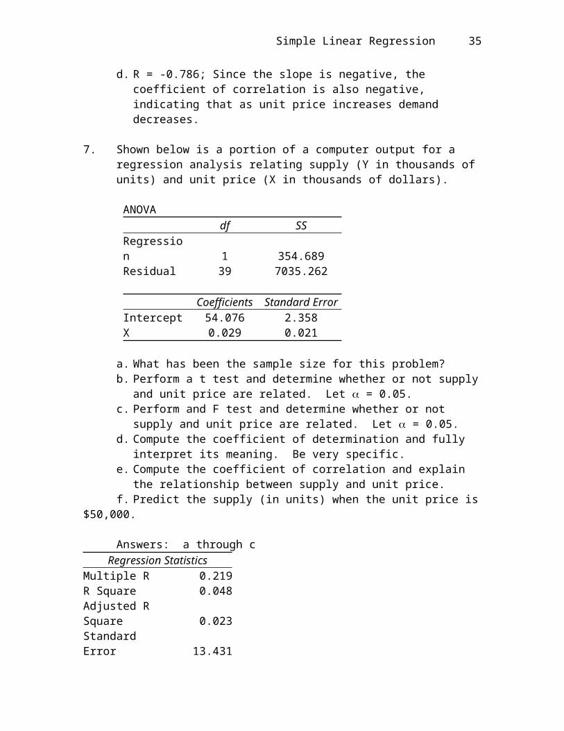
d. R = -0.786; Since the slope is negative, the coefficient of correlation is also negative, indicating that as unit price increases demand decreases.
7. Shown below is a portion of a computer output for a regression analysis relating supply (Y in thousands of units) and unit price (X in thousands of dollars).
ANOVA df SS
Regression 1 354.689Residual 39 7035.262
Coefficients Standard ErrorIntercept 54.076 2.358X 0.029 0.021
a. What has been the sample size for this problem?b. Perform a t test and determine whether or not supply and unit price are
related. Let = 0.05.c. Perform and F test and determine whether or not supply and unit price are
related. Let = 0.05.d. Compute the coefficient of determination and fully interpret its meaning. Be
very specific.e. Compute the coefficient of correlation and explain the relationship between
supply and unit price.f. Predict the supply (in units) when the unit price is $50,000.
Answers: a through cRegression Statistics
Multiple R 0.219R Square 0.048Adjusted R Square 0.023Standard Error 13.431Observations 41
ANOVA df SS MS F Significance F
Regression 1 354.689 354.689 1.966 0.169Residual 39 7035.262 180.391Total 40 7389.951
Coefficients Standard Error t Stat P-valueIntercept 54.076 2.358 22.938 0.000X 0.029 0.021 1.402 0.169

28 Chapter Fourteen
d. R2 = 0.048; 4.8% of the variability in supply is explained by the variability in price.
e. R = 0.219; Since the slope is positive, as unit price increases so does supply.f. supply = 54.076 + .029(50) = 55.526 (55,526 units)
8. Given below are five observations collected in a regression study on two variables x (independent variable) and y (dependent variable).
x y2 46 79 89 9
a. Develop the least squares estimated regression equation.b. At 95% confidence, perform a t test and determine whether or not the slope is
significantly different from zero.c. Perform an F test to determine whether or not the model is significant. Let
= 0.05.d. Compute the coefficient of determination.
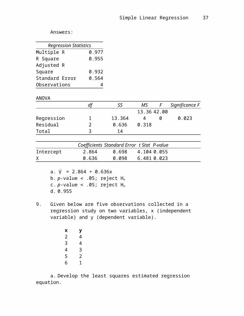
Answers:
Regression StatisticsMultiple R 0.977R Square 0.955Adjusted R Square 0.932Standard Error 0.564Observations 4
ANOVA df SS MS F Significance F
Regression 1 13.364 13.364 42.000 0.023Residual 2 0.636 0.318Total 3 14
Coefficients Standard Error t Stat P-valueIntercept 2.864 0.698 4.104 0.055X 0.636 0.098 6.481 0.023
a. = 2.864 + 0.636xb. p-value .05; reject Ho
c. p-value .05; reject Ho
d. 0.955
Simple Linear Regression 29
9. Given below are five observations collected in a regression study on two variables, x (independent variable) and y (dependent variable).
x y2 43 44 35 26 1
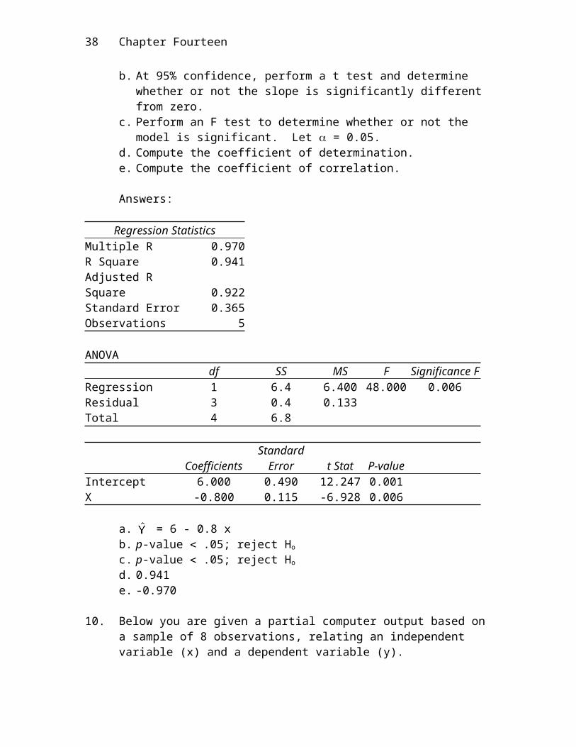
a. Develop the least squares estimated regression equation.b. At 95% confidence, perform a t test and determine whether or not the slope is
significantly different from zero.c. Perform an F test to determine whether or not the model is significant. Let
= 0.05.d. Compute the coefficient of determination.e. Compute the coefficient of correlation.
Answers:
Regression StatisticsMultiple R 0.970R Square 0.941Adjusted R Square 0.922Standard Error 0.365Observations 5
ANOVA df SS MS F Significance F
Regression 1 6.4 6.400 48.000 0.006Residual 3 0.4 0.133Total 4 6.8
Coefficients Standard Error t Stat P-valueIntercept 6.000 0.490 12.247 0.001X -0.800 0.115 -6.928 0.006
a. = 6 - 0.8 xb. p-value .05; reject Ho
c. p-value .05; reject Ho
d. 0.941e. -0.970
30 Chapter Fourteen
10. Below you are given a partial computer output based on a sample of 8 observations, relating an independent variable (x) and a dependent variable (y).
Coefficient Standard ErrorIntercept 13.251 10.77
X 0.803 0.385
Analysis of Variance
SOURCE SSRegressionError (Residual) 41.674Total 71.875
a. Develop the estimated regression line.b. At = 0.05, test for the significance of the slope.c. At = 0.05, perform an F test.d. Determine the coefficient of determination.
Answers:a. = 13.251 + 0.803xb. t = 2.086; p-value is between .05 and .1 (critical t = 2.447); do not reject Ho
c. F = 4.348; p-value is between .05 and .1 (critical F = 5.99); do not reject Ho
d. 0.42
11. Below you are given a partial computer output based on a sample of 7 observations, relating an independent variable (x) and a dependent variable (y).
Coefficient Standard ErrorIntercept -9.462 7.032
x 0.769 0.184
Analysis of Variance
SOURCE SSRegression 400Error (Residual) 138
a. Develop the estimated regression line.b. At = 0.05, test for the significance of the slope.c. At = 0.05, perform an F test.d. Determine the coefficient of determination.
Answers:a. = -9.462 + 0.769xb. t = 4.17; p-value .01; reject Ho
Simple Linear Regression 31
c. F = 17.39; p-value .01; reject Ho
d. 0.743
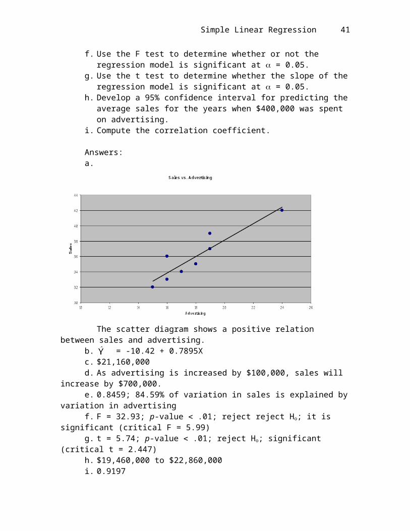
12. The following data represent a company's yearly sales volume and its advertising expenditure over a period of 8 years.
(Y) (X)Sales in Advertising
Millions of Dollars in ($10,000)15 3216 3318 3517 3416 3619 3719 3924 42
a. Develop a scatter diagram of sales versus advertising and explain what it shows regarding the relationship between sales and advertising.
b. Use the method of least squares to compute an estimated regression line between sales and advertising.
c. If the company's advertising expenditure is $400,000, what are the predicted sales? Give the answer in dollars.
d. What does the slope of the estimated regression line indicate?e. Compute the coefficient of determination and fully interpret its meaning.f. Use the F test to determine whether or not the regression model is significant
at = 0.05.g. Use the t test to determine whether the slope of the regression model is
significant at = 0.05.h. Develop a 95% confidence interval for predicting the average sales for the
years when $400,000 was spent on advertising.i. Compute the correlation coefficient.
Answers:a.
32 Chapter Fourteen
The scatter diagram shows a positive relation between sales and advertising.b. = -10.42 + 0.7895Xc. $21,160,000d. As advertising is increased by $100,000, sales will increase by $700,000.e. 0.8459; 84.59% of variation in sales is explained by variation in advertisingf. F = 32.93; p-value .01; reject reject Ho; it is significant (critical F = 5.99)g. t = 5.74; p-value .01; reject Ho; significant (critical t = 2.447)h. $19,460,000 to $22,860,000i. 0.9197
13. Given below are five observations collected in a regression study on two variables x (independent variable) and y (dependent variable).
x y10 720 530 440 250 1
a. Develop the least squares estimated regression equationb. At 95% confidence, perform a t test and determine whether or not the slope is
significantly different from zero.c. Perform an F test to determine whether or not the model is significant. Let
= 0.05.d. Compute the coefficient of determination.e. Compute the coefficient of correlation.
Answers:
Simple Linear Regression 33
a. = 8.3 – 0.15xb. t = -15; p-value < .01 (almost zero); reject Ho (critical t = 3.18)c. F = 225; p-value .01 (almost zero); reject Ho (critical F = 10.13)d. 0.9868e. 0.9934
14. Below you are given a partial computer output based on a sample of 14 observations, relating an independent variable (x) and a dependent variable (y).
Predictor Coefficient Standard ErrorConstant 6.428 1.202
X 0.470 0.035
Analysis of Variance
SOURCE SSRegression 958.584Error (Residual)Total 1021.429
a. Develop the estimated regression line.b. At = 0.05, test for the significance of the slope.c. At = 0.05, perform an F test.d. Determine the coefficient of determination.e. Determine the coefficient of correlation.
Answers:a. = 6.428 + 0.47xb. t = 13.529; p-value .01 (almost zero); reject Ho (critical t = 2.179)c. F = 183.04; p-value .01 (almost zero); reject Ho (critical F = 4.75)d. 0.938e. 0.968
15. Below you are given a partial computer output based on a sample of 21 observations, relating an independent variable (x) and a dependent variable (y).
Predictor Coefficient Standard ErrorConstant 30.139 1.181
X -0.252 0.022
Analysis of Variance
SOURCE SSRegression 1,759.481Error 259.186

34 Chapter Fourteen
a. Develop the estimated regression line.b. At = 0.05, test for the significance of the slope.c. At = 0.05, perform an F test.d. Determine the coefficient of determination.e. Determine the coefficient of correlation.
Answers:a. = 30.139 - 0.252xb. t = -11.357; p-value .01 (almost zero); reject Ho (critical t = 2.093)c. F = 128.982; p-value .01 (almost zero); reject Ho (critical F = 4.38)d. 0.872e. -0.934
16. An automobile dealer wants to see if there is a relationship between monthly sales and the interest rate. A random sample of 4 months was taken. The results of the sample are presented below. The estimated least squares regression equation is
Y XMonthly Sales Interest Rate (In Percent)
22 9.220 7.610 10.445 5.3
a. Obtain a measure of how well the estimated regression line fits the data.b. You want to test to see if there is a significant relationship between the
interest rate and monthly sales at the 1% level of significance. State the null and alternative hypotheses.
c. At 99% confidence, test the hypotheses.d. Construct a 99% confidence interval for the average monthly sales for all
months with a 10% interest rate.e. Construct a 99% confidence interval for the monthly sales of one month with
a 10% interest rate.
Answers:a. R2 = 0.8687b. H0: 1 = 0
Ha: 1 0c. test statistic t = -3.64; p-value is between .05 and .10 (critical t = 9.925); do
not reject H0
d. -33.151 to 58.199; therefore, 0 to 58.199e. -67.068 to 92.116; therefore, 0 to 92.116
17. Max believes that the sales of coffee at his coffee shop depend upon the weather.
Simple Linear Regression 35
He has taken a sample of 5 days. Below you are given the results of the sample.
Cups of Coffee Sold Temperature350 50200 60210 70100 8060 9040 100
a. Which variable is the dependent variable?b. Compute the least squares estimated line.c. Compute the correlation coefficient between temperature and the sales of
coffee.d. Is there a significant relationship between the sales of coffee and temperature?
Use a .05 level of significance. Be sure to state the null and alternative hypotheses.
e. Predict sales of a 90 degree day.
Answers:a. Salesb. = 605.714 - 5.943Xc. 0.95197d. H0: 1 = 0
Ha: 1 0t = -6.218; p-value < .01; reject Ho (critical t = 2.776)
e. 70.8 or 71 cups
18. Researchers have collected data on the hours of television watched in a day and the age of a person. You are given the data below.
Hours of Television Age1 453 304 223 256 5
a. Determine which variable is the dependent variable.b. Compute the least squares estimated line.c. Is there a significant relationship between the two variables? Use a .05 level
of significance. Be sure to state the null and alternative hypotheses.d. Compute the coefficient of determination. How would you interpret this
value?
Answers:

36 Chapter Fourteen
a. Hours of Televisionb. = 6.564 - 0.1246Xc. H0: 1 = 0
Ha: 1 0t = -12.018; p-value < .01; reject H0 (critical t = 3.18)
d. 0.98 (rounded); 98 % of variation in hours of watching television is explained by variation in age.
19. Given below are seven observations collected in a regression study on two variables, X (independent variable) and Y (dependent variable).
X Y2 123 96 87 78 67 59 2
a. Develop the least squares estimated regression equation.b. At 95% confidence, perform a t test and determine whether or not the slope is
significantly different from zero.c. Perform an F test to determine whether or not the model is significant. Let
= 0.05.d. Compute the coefficient of determination.
Answers:a. Ŷ = 13.75 -1.125Xb. t = -5.196; p-value < .01; reject Ho (critical t = 2.571)c. F = 27; p-value .01; reject Ho (critical F = 6.61)d. 0.844
20. The owner of a retail store randomly selected the following weekly data on profits and advertising cost.
Week Advertising Cost ($) Profit ($)1 0 2002 50 2703 250 4204 150 3005 125 325
a. Write down the appropriate linear relationship between advertising cost and profits. Which is the dependent variable? Which is the independent variable?
b. Calculate the least squares estimated regression line.
Simple Linear Regression 37
c. Predict the profits for a week when $200 is spent on advertising.d. At 95% confidence, test to determine if the relationship between advertising
costs and profits is statistically significant.e. Calculate the coefficient of determination.
Answers:a. E(Y) = 0 + 1 where Y is profit and X is advertising costb. = 210.0676 + 0.80811Xc. $371.69d. t = 6.496; p-value .01; reject Ho; relationship is significant (critical t =
3.182)e. 0.9336
21. The owner of a bakery wants to analyze the relationship between the expenditure of a customer and the customer's income. A sample of 5 customers is taken and the following information was obtained.
Y XExpenditure Income (In Thousands)
.45 2010.75 195.40 227.80 255.60 14
The least squares estimated line is = 4.348 + 0.0826 X.a. Obtain a measure of how well the estimated regression line fits the data.b. You want to test to see if there is a significant relationship between
expenditure and income at the 5% level of significance. Be sure to state the null and alternative hypotheses.
c. Construct a 95% confidence interval estimate for the average expenditure for all customers with an income of $20,000.
d. Construct a 95% confidence interval estimate for the expenditure of one customer whose income is $20,000.
Answers:a. R2 = 0.0079b. H0: 1 = 0
Ha: 1 0t = 0.154; p-value 0.1; do not reject H0; (critical t = 3.182)
c. 0.185 to 12.185d. -9.151 to 21.151
22. Below you are given information on annual income and years of college education.
38 Chapter Fourteen
Income (In Thousands) Years of College28 040 336 228 148 4
a. Develop the least squares regression equation.b. Estimate the yearly income of an individual with 6 years of college education.c. Compute the coefficient of determination.d. Use a t test to determine whether the slope is significantly different from zero.
Let = 0.05.e. At 95% confidence, perform an F test and determine whether or not the model
is significant.
Answers:a. = 25.6 + 5.2Xb. $56,800c. 0.939d. t = 6.789; p-value .01; reject Ho; significant (critical t = 3.182e. F = 46.091; p-value .01; reject Ho; significant (critical F = 10.13)
23. Below you are given information on a woman's age and her annual expenditure on purchase of books.
Age Annual Expenditure ($)18 21022 18021 22028 280
a. Develop the least squares regression equation.b. Compute the coefficient of determination.c. Use a t test to determine whether the slope is significantly different from zero.
Let = 0.05.d. At 95% confidence, perform an F test and determine whether or not the model
is significant.
Answers:a. = 54.834 + 7.536Xb. R2 = 0.568c. t = 1.621; p-value 0.1; do not reject Ho; not significant (critical t = 4.303)d. F = 2.628; p-value 0.1; do not reject Ho; not significant (critical F = 18.51)
24. The following sample data contains the number of years of college and the current annual salary for a random sample of heavy equipment salespeople.

Simple Linear Regression 39
Years of College Annual Income (In Thousands)2 202 233 254 263 281 294 273 304 334 35
a. Which variable is the dependent variable? Which is the independent variable?b. Determine the least squares estimated regression line.c. Predict the annual income of a salesperson with one year of college.d. Test if the relationship between years of college and income is statistically
significant at the .05 level of significance.e. Calculate the coefficient of determination.f. Calculate the sample correlation coefficient between income and years of
college. Interpret the value you obtain.
Answers:a. Y (dependent variable) is annual income and X (independent variable) is
years of collegeb. = 21.6 + 2Xc. $23,600d. The relationship is not statistically significant since t = 1.51; p-value 0.1
(critical t = 2.306)e. 0.222f. 0.471; there is a positive correlation between years of college and annual
income
25. The following data shows the yearly income (in $1,000) and age of a sample of seven individuals.
Income (in $1,000) Age20 1824 2024 2325 3426 2427 2734 27
a. Develop the least squares regression equation.

40 Chapter Fourteen
b. Estimate the yearly income of a 30-year-old individual.c. Compute the coefficient of determination.d. Use a t test to determine whether the slope is significantly different from zero.
Let = 0.05.e. At 95% confidence, perform an F test and determine whether or not the model
is significant.
Answers:a. = 16.204 + 0.3848Xb. $27,748c. 0.2266d. t = 1.21; p-value 0.1; not significant (critical t = 2.571)e. F = 1.46; p-value 0.1; not significant (critical F = 6.61)
26. The following data show the results of an aptitude test (Y) and the grade point average of 10 students.
Aptitude TestScore (Y) GPA (X)
26 1.831 2.328 2.630 2.434 2.838 3.041 3.444 3.240 3.643 3.8
a. Develop a least squares estimated regression line.b. Compute the coefficient of determination and comment on the strength of the
regression relationship.c. Is the slope significant? Use a t test and let = 0.05.d. At 95% confidence, test to determine if the model is significant (i.e., perform
an F test).
Answers:a. = 8.171 + 9.4564Xb. 0.83; there is a fairly strong relationshipc. t = 6.25; p-value .01; it is significant (critical t = 2.306)d. F = 39.07; p-value .01; it is significant (critical F = 5.32)
27. Shown below is a portion of the computer output for a regression analysis relating sales (Y in millions of dollars) and advertising expenditure (X in thousands of dollars).
Simple Linear Regression 41
Predictor Coefficient Standard ErrorConstant 4.00 0.800
X 0.12 0.045
Analysis of Variance
SOURCE DF SSRegression 1 1,400Error 18 3,600
a. What has been the sample size for the above?b. Perform a t test and determine whether or not advertising and sales are
related. Let = 0.05.c. Compute the coefficient of determination.d. Interpret the meaning of the value of the coefficient of determination that you
found in Part c. Be very specific.e. Use the estimated regression equation and predict sales for an advertising
expenditure of $4,000. Give your answer in dollars.
Answers:a. 20b. t = 2.66; p-value is between 0.01 and 0.02; they are related (critical t = 2.101)c. R2 = 0.28d. 28% of variation in sales is explained by variation in advertising expenditure.e. $4,480,000
28. A company has recorded data on the daily demand for its product (Y in thousands of units) and the unit price (X in hundreds of dollars). A sample of 15 days demand and associated prices resulted in the following data.
X = 75 = -59Y = 135 = 94 = 100SSE = 62.9681
a. Using the above information, develop the least-squares estimated regression line and write the equation.
b. Compute the coefficient of determination.c. Perform an F test and determine whether or not there is a significant
relationship between demand and unit price. Let = 0.05.d. Would the demand ever reach zero? If yes, at what price would the demand
be zero?
Answers:a. = 12.138 – 0.6277

42 Chapter Fourteen
b. R2 = 0.3703c. F = 7.65; p-value is between .01 and .025; reject Ho and conclude that demand
and unit price are related (critical F = 4.67)d. Yes, at $1,934