SAS/STAT ® 12.3 User’s Guide High-Performance Procedures

Welcome message from author
This document is posted to help you gain knowledge. Please leave a comment to let me know what you think about it! Share it to your friends and learn new things together.
Transcript
SAS/STAT® 12.3User’s GuideHigh-Performance Procedures

The correct bibliographic citation for this manual is as follows: SAS Institute Inc. 2013. SAS/STAT® 12.3 User’s Guide:High-Performance Procedures. Cary, NC: SAS Institute Inc.
SAS/STAT® 12.3 User’s Guide: High-Performance Procedures
Copyright © 2013, SAS Institute Inc., Cary, NC, USA
All rights reserved. Produced in the United States of America.
For a hard-copy book: No part of this publication may be reproduced, stored in a retrieval system, or transmitted, in any form orby any means, electronic, mechanical, photocopying, or otherwise, without the prior written permission of the publisher, SASInstitute Inc.
For a web download or e-book: Your use of this publication shall be governed by the terms established by the vendor at the timeyou acquire this publication.
The scanning, uploading, and distribution of this book via the Internet or any other means without the permission of the publisher isillegal and punishable by law. Please purchase only authorized electronic editions and do not participate in or encourage electronicpiracy of copyrighted materials. Your support of others’ rights is appreciated.
U.S. Government Restricted Rights Notice: Use, duplication, or disclosure of this software and related documentation by theU.S. government is subject to the Agreement with SAS Institute and the restrictions set forth in FAR 52.227-19, CommercialComputer Software–Restricted Rights (June 1987).
SAS Institute Inc., SAS Campus Drive, Cary, North Carolina 27513.
July 2013
SAS provides a complete selection of books and electronic products to help customers use SAS® software to its fullest potential.For more information about our e-books, e-learning products, CDs, and hard-copy books, visit support.sas.com/bookstore orcall 1-800-727-3228.
SAS® and all other SAS Institute Inc. product or service names are registered trademarks or trademarks of SAS Institute Inc. inthe USA and other countries. ® indicates USA registration.
Other brand and product names are registered trademarks or trademarks of their respective companies.

ContentsChapter 1. Introduction . . . . . . . . . . . . . . . . . . . . . . . . . . . 1Chapter 2. Shared Concepts and Topics . . . . . . . . . . . . . . . . . . . . . 5Chapter 3. Shared Statistical Concepts . . . . . . . . . . . . . . . . . . . . . 39Chapter 4. The HPGENSELECT Procedure . . . . . . . . . . . . . . . . . . . 71Chapter 5. The HPLOGISTIC Procedure . . . . . . . . . . . . . . . . . . . . 127Chapter 6. The HPLMIXED Procedure . . . . . . . . . . . . . . . . . . . . . 185Chapter 7. The HPNLMOD Procedure . . . . . . . . . . . . . . . . . . . . . 227Chapter 8. The HPREG Procedure . . . . . . . . . . . . . . . . . . . . . . . 263Chapter 9. The HPSPLIT Procedure . . . . . . . . . . . . . . . . . . . . . . 309
Subject Index 345
Syntax Index 353

iv
Credits and Acknowledgments
Credits
DocumentationEditing Anne Baxter, Ed Huddleston
Documentation Support Tim Arnold
SoftwareThe procedures in this book were implemented by the following members of the development staff. Programdevelopment includes design, programming, debugging, support, and documentation. In the following list,the names of the developers who currently provide primary support are listed first; other developers andprevious developers are also listed.
HPGENSELECT Gordon JohnstonHPLMIXED Tianlin Wang, Biruk GebramariamHPLOGISTIC Robert E. Derr, Oliver SchabenbergerHPNLMOD Marc Kessler, Oliver SchabenbergerHPREG Robert CohenHPSPLIT Joseph PingenotHigh-performance computing foundation Steve E. KruegerHigh-performance analytics foundation Robert Cohen, Georges H. Guirguis, Trevor
Kearney, Richard Knight, Gang Meng, OliverSchabenberger, Charles Shorb, Tom P. Weber
Numerical routines Georges H. Guirguis
The following people contribute with their leadership and support: Chris Bailey, Tanya Balan, David Pope,Oliver Schabenberger, Renee Sciortino.
TestingJack Berry, Tim Carter, Enzo D’Andreti, Girija Gavankar, Greg Goodwin, Dright Ho, Seungho Huh, GerardoHurtado, Cheryl LeSaint, Yu Liang, Jim McKenzie, Jim Metcalf, Huiping Miao, Bengt Pederson, JaymieShanahan, Fouad Younan.

Internationalization TestingFeng Gao, Alex(Wenqi) He, David Li, Frank(Jidong) Wang, Lina Xu.
Technical SupportPhil Gibbs
AcknowledgmentsMany people make significant and continuing contributions to the development of SAS software products.
The final responsibility for the SAS System lies with SAS alone. We hope that you will always let us knowyour opinions about the SAS System and its documentation. It is through your participation that SAS softwareis continuously improved.
vi
Chapter 1
Introduction
ContentsOverview of SAS/STAT High-Performance Procedures . . . . . . . . . . . . . . . . . . . . 1About This Book . . . . . . . . . . . . . . . . . . . . . . . . . . . . . . . . . . . . . . . . 1
Chapter Organization . . . . . . . . . . . . . . . . . . . . . . . . . . . . . . . . . . 1Typographical Conventions . . . . . . . . . . . . . . . . . . . . . . . . . . . . . . . 2Options Used in Examples . . . . . . . . . . . . . . . . . . . . . . . . . . . . . . . . 2
Online Documentation . . . . . . . . . . . . . . . . . . . . . . . . . . . . . . . . . . . . . 3SAS Technical Support Services . . . . . . . . . . . . . . . . . . . . . . . . . . . . . . . . 3
Overview of SAS/STAT High-Performance ProceduresSAS/STAT high-performance procedures provide predictive modeling tools that have been specially developedto take advantage of parallel processing in both multithreaded single-machine mode and distributed multiple-machine mode. Predictive modeling methods include regression, logistic regression, generalized linearmodels, linear mixed models, nonlinear models, and decision trees. The procedures provide model selection,dimension reduction, and identification of important variables whenever this is appropriate for the analysis.
In addition to the high-performance statistical procedures described in this book, SAS/STAT includes high-performance utility procedures, which are described in Base SAS Procedures Guide: High-Performance Pro-cedures. You can run all these procedures in single-machine mode without licensing SAS High-PerformanceStatistics. However, to run these procedures in distributed mode, you must license SAS High-PerformanceStatistics.
About This BookThis book assumes that you are familiar with Base SAS software and with the books SAS Language Reference:Concepts and Base SAS Procedures Guide. It also assumes that you are familiar with basic SAS Systemconcepts, such as using the DATA step to create SAS data sets and using Base SAS procedures (such as thePRINT and SORT procedures) to manipulate SAS data sets.
Chapter OrganizationThis book is organized as follows:

2 F Chapter 1: Introduction
Chapter 1, this chapter, provides an overview of SAS/STAT high-performance procedures.
Chapter 2, “Shared Concepts and Topics,” describes the modes in which SAS/STAT high-performanceprocedures can execute.
Chapter 3, “Shared Statistical Concepts,” describes common syntax elements that are supported by SAS/STAThigh-performance procedures.
Subsequent chapters describe the individual procedures. These chapters appear in alphabetical order byprocedure name. Each chapter is organized as follows:
• The “Overview” section provides a brief description of the analysis provided by the procedure.
• The “Getting Started” section provides a quick introduction to the procedure through a simple example.
• The “Syntax” section describes the SAS statements and options that control the procedure.
• The “Details” section discusses methodology and other topics, such as ODS tables.
• The “Examples” section contains examples that use the procedure.
• The “References” section contains references for the methodology.
Typographical ConventionsThis book uses several type styles for presenting information. The following list explains the meaning of thetypographical conventions used in this book:
roman is the standard type style used for most text.
UPPERCASE ROMAN is used for SAS statements, options, and other SAS language elements whenthey appear in the text. However, you can enter these elements in your own SASprograms in lowercase, uppercase, or a mixture of the two.
UPPERCASE BOLD is used in the “Syntax” sections’ initial lists of SAS statements and options.
oblique is used in the syntax definitions and in text to represent arguments for which yousupply a value.
VariableName is used for the names of variables and data sets when they appear in the text.
bold is used to for matrices and vectors.
italic is used for terms that are defined in the text, for emphasis, and for references topublications.
monospace is used for example code. In most cases, this book uses lowercase type for SAScode.
Options Used in ExamplesMost of the output shown in this book is produced with the following SAS System options:

Online Documentation F 3
options linesize=80 pagesize=500 nonumber nodate;
The HTMLBLUE style is used to create the HTML output and graphs that appear in the online documentation.A style template controls stylistic elements such as colors, fonts, and presentation attributes. The styletemplate is specified in the ODS HTML statement as follows:
ods html style=HTMLBlue;
If you run the examples, your output might be slightly different, because of the SAS System options you useand the precision that your computer uses for floating-point calculations.
Online DocumentationThis documentation is available online with the SAS System. To access documentation for the SAS/STAThigh-performance procedures from the SAS windowing environment, select Help from the main menu andthen select SAS Help and Documentation. On the Contents tab, expand the SAS Products, SAS/STAT,and SAS/STAT User’s Guide: High-Performance Procedures items. Then expand chapters and click onsections. You can search the documentation by using the Search tab.
You can also access the documentation by going to http://support.sas.com/documentation.
SAS Technical Support ServicesThe SAS Technical Support staff is available to respond to problems and answer technical questions re-garding the use of high-performance procedures. Go to http://support.sas.com/techsup for moreinformation.

4
Chapter 2
Shared Concepts and Topics
ContentsOverview . . . . . . . . . . . . . . . . . . . . . . . . . . . . . . . . . . . . . . . . . . . . 5Processing Modes . . . . . . . . . . . . . . . . . . . . . . . . . . . . . . . . . . . . . . . . 6
Single-Machine Mode . . . . . . . . . . . . . . . . . . . . . . . . . . . . . . . . . . 6Distributed Mode . . . . . . . . . . . . . . . . . . . . . . . . . . . . . . . . . . . . . 6Symmetric and Asymmetric Distributed Modes . . . . . . . . . . . . . . . . . . . . . 7Controlling the Execution Mode with Environment Variables and Performance State-
ment Options . . . . . . . . . . . . . . . . . . . . . . . . . . . . . . . . . . 7Determining Single-Machine Mode or Distributed Mode . . . . . . . . . . . . . . . . 9
Alongside-the-Database Execution . . . . . . . . . . . . . . . . . . . . . . . . . . . . . . . 13Alongside-LASR Distributed Execution . . . . . . . . . . . . . . . . . . . . . . . . . . . . 16Running High-Performance Analytical Procedures Alongside a SAS LASR Analytic Server
in Distributed Mode . . . . . . . . . . . . . . . . . . . . . . . . . . . . . . . . . . . 17Starting a SAS LASR Analytic Server Instance . . . . . . . . . . . . . . . . . . . . . 17Associating a SAS Libref with the SAS LASR Analytic Server Instance . . . . . . . . 18Running a High-Performance Analytical Procedure Alongside the SAS LASR Analytic
Server Instance . . . . . . . . . . . . . . . . . . . . . . . . . . . . . . . . . 18Terminating a SAS LASR Analytic Server Instance . . . . . . . . . . . . . . . . . . . 19
Alongside-LASR Distributed Execution on a Subset of the Appliance Nodes . . . . . . . . . 19Running High-Performance Analytical Procedures in Asymmetric Mode . . . . . . . . . . . 19
Running in Symmetric Mode . . . . . . . . . . . . . . . . . . . . . . . . . . . . . . 20Running in Asymmetric Mode on One Appliance . . . . . . . . . . . . . . . . . . . . 21Running in Asymmetric Mode on Distinct Appliances . . . . . . . . . . . . . . . . . 22
Alongside-HDFS Execution . . . . . . . . . . . . . . . . . . . . . . . . . . . . . . . . . . 25Alongside-HDFS Execution by Using the SASHDAT Engine . . . . . . . . . . . . . 25Alongside-HDFS Execution by Using the Hadoop Engine . . . . . . . . . . . . . . . 27
Output Data Sets . . . . . . . . . . . . . . . . . . . . . . . . . . . . . . . . . . . . . . . . 31Working with Formats . . . . . . . . . . . . . . . . . . . . . . . . . . . . . . . . . . . . . 32PERFORMANCE Statement . . . . . . . . . . . . . . . . . . . . . . . . . . . . . . . . . . 34
OverviewThis chapter describes the modes of execution in which SAS high-performance analytical procedures canexecute. If you have SAS/STAT installed, you can run any procedure in this book on a single machine.
6 F Chapter 2: Shared Concepts and Topics
However, to run procedures in this book in distributed mode, you must also have SAS High-PerformanceStatistics software installed. For more information about these modes, see the next section.
This chapter provides details of how you can control the modes of execution and includes the syntax for thePERFORMANCE statement, which is common to all high-performance analytical procedures.
Processing Modes
Single-Machine ModeSingle-machine mode is a computing model in which multiple processors or multiple cores are controlledby a single operating system and can access shared resources, such as disks and memory. In this book,single-machine mode refers to an application running multiple concurrent threads on a multicore machinein order to take advantage of parallel execution on multiple processing units. More simply, single-machinemode for high-performance analytical procedures means multithreading on the client machine.
All high-performance analytical procedures are capable of running in single-machine mode, and this is thedefault mode when a procedure runs on the client machine. The procedure uses the number of CPUs (cores)on the machine to determine the number of concurrent threads. High-performance analytical procedures usedifferent methods to map core count to the number of concurrent threads, depending on the analytic task.Using one thread per core is not uncommon for the procedures that implement data-parallel algorithms.
Distributed ModeDistributed mode is a computing model in which several nodes in a distributed computing environmentparticipate in the calculations. In this book, the distributed mode of a high-performance analytical procedurerefers to the procedure performing the analytics on an appliance that consists of a cluster of nodes. Thisappliance can be one of the following:
• a database management system (DBMS) appliance on which the SAS High-Performance Analyticsinfrastructure is also installed
• a cluster of nodes that have the SAS High-Performance Analytics infrastructure installed but no DBMSsoftware installed
Distributed mode has several variations:
• Client-data (or local-data) mode: The input data for the analytic task are not stored on the appliance orcluster but are distributed to the distributed computing environment by the SAS High-PerformanceAnalytics infrastructure when the procedure runs.
• Alongside-the-database mode: The data are stored in the distributed database and are read from theDBMS in parallel into a high-performance analytical procedure that runs on the database appliance.
Symmetric and Asymmetric Distributed Modes F 7
• Alongside-HDFS mode: The data are stored in the Hadoop Distributed File System (HDFS) andare read in parallel from the HDFS. This mode is available if you install the SAS High-PerformanceDeployment of Hadoop on the appliance or when you configure a Cloudera 4 Hadoop deployment on theappliance to operate with the SAS High-Performance Analytics infrastructure. For more informationabout installing the SAS High-Performance Deployment of Hadoop, see the SAS High-PerformanceAnalytics Infrastructure: Installation and Configuration Guide.
• Alongside-LASR mode: The data are loaded from a SAS LASR Analytic Server that runs on theappliance.
Symmetric and Asymmetric Distributed ModesSAS high-performance analytical procedures can run alongside the database or alongside HDFS in asymmetricmode. The primary reason for providing the asymmetric mode is to enable you to manage and house dataon one appliance (the data appliance) and to run the high-performance analytical procedure on a secondappliance (the computing appliance). You can also run in asymmetric mode on a single appliance thatfunctions as both the data appliance and the computing appliance. This enables you to run alongside thedatabase or alongside HDFS, where computations are done on a different set of nodes from the nodes thatcontain the data. The following subsections provide more details.
Symmetric ModeWhen SAS high-performance analytical procedures run in symmetric distributed mode, the data applianceand the computing appliance must be the same appliance. Both the SAS Embedded Process and the high-performance analytical procedures execute in a SAS process that runs on the same hardware where theDBMS process executes. This is called symmetric mode because the number of nodes on which the DBMSexecutes is the same as the number of nodes on which the high-performance analytical procedures execute.The initial data movement from the DBMS to the high-performance analytical procedure does not cross nodeboundaries.
Asymmetric ModeWhen SAS high-performance analytical procedures run in asymmetric distributed mode, the data applianceand computing appliance are usually distinct appliances. The high-performance analytical procedures executein a SAS process that runs on the computing appliance. The DBMS and a SAS Embedded Process runon the data appliance. Data are requested by a SAS data feeder that runs on the computing appliance andcommunicates with the SAS Embedded Process on the data appliance. The SAS Embedded Process transfersthe data in parallel to the SAS data feeder that runs on each of the nodes of the computing appliance. This iscalled asymmetric mode because the number of nodes on the data appliance does not need to be the same asthe number of nodes on the computing appliance.
Controlling the Execution Mode with Environment Variables andPerformance Statement OptionsYou control the execution mode by using environment variables or by specifying options in the PERFOR-MANCE statement in high-performance analytical procedures, or by a combination of these methods.
8 F Chapter 2: Shared Concepts and Topics
The important environment variables follow:
• grid host identifies the domain name system (DNS) or IP address of the appliance node to which theSAS High-Performance Statistics software connects to run in distributed mode.
• installation location identifies the directory where the SAS High-Performance Statistics software isinstalled on the appliance.
• data server identifies the database server on Teradata appliances as defined in the hosts file on the client.This data server is the same entry that you usually specify in the SERVER= entry of a LIBNAMEstatement for Teradata. For more information about specifying LIBNAME statements for Teradata andother engines, see the DBMS-specific section of SAS/ACCESS for Relational Databases: Referencefor your engine.
• grid mode specifies whether the high-performance analytical procedures execute in symmetric orasymmetric mode. Valid values for this variable are 'sym' for symmetric mode and 'asym' forasymmetric mode. The default is symmetric mode.
You can set an environment variable directly from the SAS program by using the OPTION SET= command.For example, the following statements define three variables for a Teradata appliance (the grid mode is thedefault symmetric mode):
option set=GRIDHOST ="hpa.sas.com";option set=GRIDINSTALLLOC="/opt/TKGrid";option set=GRIDDATASERVER="myserver";
Alternatively, you can set the parameters in the PERFORMANCE statement in high-performance analyticalprocedures. For example:
performance host ="hpa.sas.com"install ="/opt/TKGrid"dataserver="myserver";
The following statements define three variables that are needed to run asymmetrically on a computingappliance.
option set=GRIDHOST ="compute_appliance.sas.com";option set=GRIDINSTALLLOC="/opt/TKGrid";option set=GRIDMODE ="asym";
Alternatively, you can set the parameters in the PERFORMANCE statement in high-performance analyticalprocedures. For example:
performance host ="compute_appliance.sas.com"install ="/opt/TKGrid"gridmode ="asym"
A specification in the PERFORMANCE statement overrides a specification of an environment variablewithout resetting its value. An environment variable that you set in the SAS session by using an OPTIONSET= command remains in effect until it is modified or until the SAS session terminates.
Determining Single-Machine Mode or Distributed Mode F 9
Specifying a data server is necessary only on Teradata systems when you do not explicitly set the gridmodeenvironment variable or specify the GRIDMODE= option in the PERFORMANCE statement. The dataserver specification depends on the entries in the (client) hosts file. The file specifies the server (suffixed bycop and a number) and an IP address. For example:
myservercop1 33.44.55.66
The key variable that determines whether a high-performance analytical procedure executes in single-machineor distributed mode is the grid host. The installation location and data server are needed to ensure that aconnection to the grid host can be made, given that a host is specified. This book assumes that the installationlocation and data server (if necessary) have been set by your system administrator.
The following sets of SAS statements are functionally equivalent:
proc hpreduce;reduce unsupervised x:;performance host="hpa.sas.com";
run;
option set=GRIDHOST="hpa.sas.com";proc hpreduce;
reduce unsupervised x:;run;
Determining Single-Machine Mode or Distributed ModeHigh-performance analytical procedures use the following rules to determine whether they run in single-machine mode or distributed mode:
• If a grid host is not specified, the analysis is carried out in single-machine mode on the client machinethat runs the SAS session.
• If a grid host is specified, the behavior depends on whether the execution is alongside the databaseor alongside HDFS. If the data are local to the client (that is, not stored in the distributed database orHDFS on the appliance), you need to use the NODES= option in the PERFORMANCE statementto specify the number of nodes on the appliance or cluster that you want to engage in the analysis.If the procedure executes alongside the database or alongside HDFS, you do not need to specify theNODES= option.
The following example shows single-machine and client-data distributed configurations for a data set of100,000 observations that are simulated from a logistic regression model. The following DATA step generatesthe data:
data simData;array _a{8} _temporary_ (0,0,0,1,0,1,1,1);array _b{8} _temporary_ (0,0,1,0,1,0,1,1);array _c{8} _temporary_ (0,1,0,0,1,1,0,1);

10 F Chapter 2: Shared Concepts and Topics
do obsno=1 to 100000;x = rantbl(1,0.28,0.18,0.14,0.14,0.03,0.09,0.08,0.06);a = _a{x};b = _b{x};c = _c{x};x1 = int(ranuni(1)*400);x2 = 52 + ranuni(1)*38;x3 = ranuni(1)*12;lp = 6. -0.015*(1-a) + 0.7*(1-b) + 0.6*(1-c) + 0.02*x1 -0.05*x2 - 0.1*x3;y = ranbin(1,1,(1/(1+exp(lp))));output;
end;drop x lp;
run;
The following statements run PROC HPLOGISTIC to fit a logistic regression model:
proc hplogistic data=simData;class a b c;model y = a b c x1 x2 x3;
run;
Figure 2.1 shows the results from the analysis.
Figure 2.1 Results from Logistic Regression in Single-Machine Mode
The HPLOGISTIC Procedure
Performance Information
Execution Mode Single-MachineNumber of Threads 4
Model Information
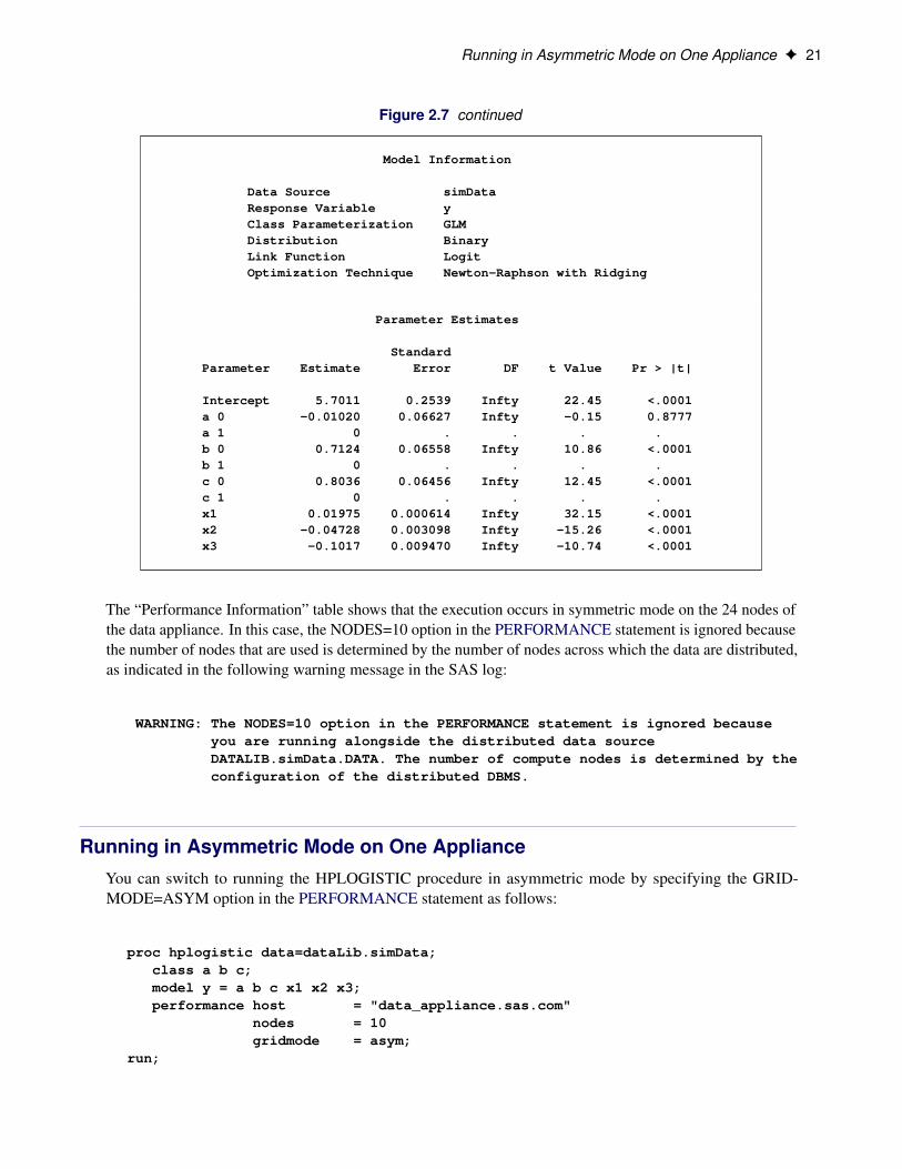
Data Source WORK.SIMDATAResponse Variable yClass Parameterization GLMDistribution BinaryLink Function LogitOptimization Technique Newton-Raphson with Ridging

Determining Single-Machine Mode or Distributed Mode F 11
Figure 2.1 continued
Parameter Estimates
StandardParameter Estimate Error DF t Value Pr > |t|
Intercept 5.7011 0.2539 Infty 22.45 <.0001a 0 -0.01020 0.06627 Infty -0.15 0.8777a 1 0 . . . .b 0 0.7124 0.06558 Infty 10.86 <.0001b 1 0 . . . .c 0 0.8036 0.06456 Infty 12.45 <.0001c 1 0 . . . .x1 0.01975 0.000614 Infty 32.15 <.0001x2 -0.04728 0.003098 Infty -15.26 <.0001x3 -0.1017 0.009470 Infty -10.74 <.0001
The entries in the “Performance Information” table show that the HPLOGISTIC procedure runs in single-machine mode and uses four threads, which are chosen according to the number of CPUs on the clientmachine. You can force a certain number of threads on any machine that is involved in the computationsby specifying the NTHREADS option in the PERFORMANCE statement. Another indication of executionon the client is the following message, which is issued in the SAS log by all high-performance analyticalprocedures:
NOTE: The HPLOGISTIC procedure is executing on the client.
The following statements use 10 nodes (in distributed mode) to analyze the data on the appliance; resultsappear in Figure 2.2:
proc hplogistic data=simData;class a b c;model y = a b c x1 x2 x3;performance host="hpa.sas.com" nodes=10;
run;
Figure 2.2 Results from Logistic Regression in Distributed Mode
The HPLOGISTIC Procedure
Performance Information
Host Node hpa.sas.comExecution Mode DistributedGrid Mode SymmetricNumber of Compute Nodes 10Number of Threads per Node 24

12 F Chapter 2: Shared Concepts and Topics
Figure 2.2 continued
Model Information
Data Source WORK.SIMDATAResponse Variable yClass Parameterization GLMDistribution BinaryLink Function LogitOptimization Technique Newton-Raphson with Ridging
Parameter Estimates
StandardParameter Estimate Error DF t Value Pr > |t|
Intercept 5.7011 0.2539 Infty 22.45 <.0001a 0 -0.01020 0.06627 Infty -0.15 0.8777a 1 0 . . . .b 0 0.7124 0.06558 Infty 10.86 <.0001b 1 0 . . . .c 0 0.8036 0.06456 Infty 12.45 <.0001c 1 0 . . . .x1 0.01975 0.000614 Infty 32.15 <.0001x2 -0.04728 0.003098 Infty -15.26 <.0001x3 -0.1017 0.009470 Infty -10.74 <.0001
The specification of a host causes the “Performance Information” table to display the name of the host nodeof the appliance. The “Performance Information” table also indicates that the calculations were performed ina distributed environment on the appliance. Twenty-four threads on each of 10 nodes were used to performthe calculations—for a total of 240 threads.
Another indication of distributed execution on the appliance is the following message, which is issued in theSAS log by all high-performance analytical procedures:
NOTE: The HPLOGISTIC procedure is executing in the distributedcomputing environment with 10 worker nodes.
You can override the presence of a grid host and force the computations into single-machine mode byspecifying the NODES=0 option in the PERFORMANCE statement:
proc hplogistic data=simData;class a b c;model y = a b c x1 x2 x3;performance host="hpa.sas.com" nodes=0;
run;
Figure 2.3 shows the “Performance Information” table. The numeric results are not reproduced here, but theyagree with the previous analyses, which are shown in Figure 2.1 and Figure 2.2.

Alongside-the-Database Execution F 13
Figure 2.3 Single-Machine Mode Despite Host Specification
The HPLOGISTIC Procedure
Performance Information
Execution Mode Single-MachineNumber of Threads 4
The “Performance Information” table indicates that the HPLOGISTIC procedure executes in single-machinemode on the client. This information is also reported in the following message, which is issued in the SASlog:
NOTE: The HPLOGISTIC procedure is executing on the client.
In the analysis shown previously in Figure 2.2, the data set Work.simData is local to the client, and theHPLOGISTIC procedure distributed the data to 10 nodes on the appliance. The High-Performance Analyticsinfrastructure does not keep these data on the appliance. When the procedure terminates, the in-memoryrepresentation of the input data on the appliance is freed.
When the input data set is large, the time that is spent sending client-side data to the appliance might dominatethe execution time. In practice, transfer speeds are usually lower than the theoretical limits of the networkconnection or disk I/O rates. At a transfer rate of 40 megabytes per second, sending a 10-gigabyte data setto the appliance requires more than four minutes. If analytic execution time is in the range of seconds, the“performance” of the process is dominated by data movement.
The alongside-the-database execution model, unique to high-performance analytical procedures, enables youto read and write data in distributed form from the database that is installed on the appliance.
Alongside-the-Database ExecutionHigh-performance analytical procedures interface with the distributed database management system (DBMS)on the appliance in a unique way. If the input data are stored in the DBMS and the grid host is the appliancethat houses the data, high-performance analytical procedures create a distributed computing environment inwhich an analytic process is co-located with the nodes of the DBMS. Data then pass from the DBMS to theanalytic process on each node. Instead of moving across the network and possibly back to the client machine,the data pass locally between the processes on each node of the appliance.
Because the analytic processes on the appliance are separate from the database processes, the technique isreferred to as alongside-the-database execution in contrast to in-database execution, where the analytic codeexecutes in the database process.
In general, when you have a large amount of input data, you can achieve the best performance fromhigh-performance analytical procedures if execution is alongside the database.

14 F Chapter 2: Shared Concepts and Topics
Before you can run alongside the database, you must distribute the data to the appliance. The followingstatements use the HPDS2 procedure to distribute the data set Work.simData into the mydb database on thehpa.sas.com appliance. In this example, the appliance houses a Greenplum database.
option set=GRIDHOST="hpa.sas.com";libname applianc greenplm
server ="hpa.sas.com"user =XXXXXXpassword=YYYYYdatabase=mydb;
proc datasets lib=applianc nolist; delete simData;proc hpds2 data=simData
out =applianc.simData(distributed_by='distributed randomly');performance commit=10000 nodes=all;data DS2GTF.out;
method run();set DS2GTF.in;
end;enddata;
run;
If the output table applianc.simData exists, the DATASETS procedure removes the table from the Greenplumdatabase because a DBMS does not usually support replacement operations on tables.
Note that the libref for the output table points to the appliance. The data set option informs the HPDS2procedure to distribute the records randomly among the data segments of the appliance. The statements thatfollow the PERFORMANCE statement are the DS2 program that copies the input data to the output datawithout further transformations.
Alongside-the-Database Execution F 15
Because you loaded the data into a database on the appliance, you can use the following HPLOGISTICstatements to perform the analysis on the appliance in the alongside-the-database mode. These statementsare almost identical to the first PROC HPLOGISTIC example in the previous section, which executed insingle-machine mode.
proc hplogistic data=applianc.simData;class a b c;model y = a b c x1 x2 x3;
run;
The subtle differences are as follows:
• The grid host environment variable that you specified in an OPTION SET= command is still in effect.
• The DATA= option in the high-performance analytical procedure uses a libref that identifies the datasource as being housed on the appliance. This libref was specified in a prior LIBNAME statement.
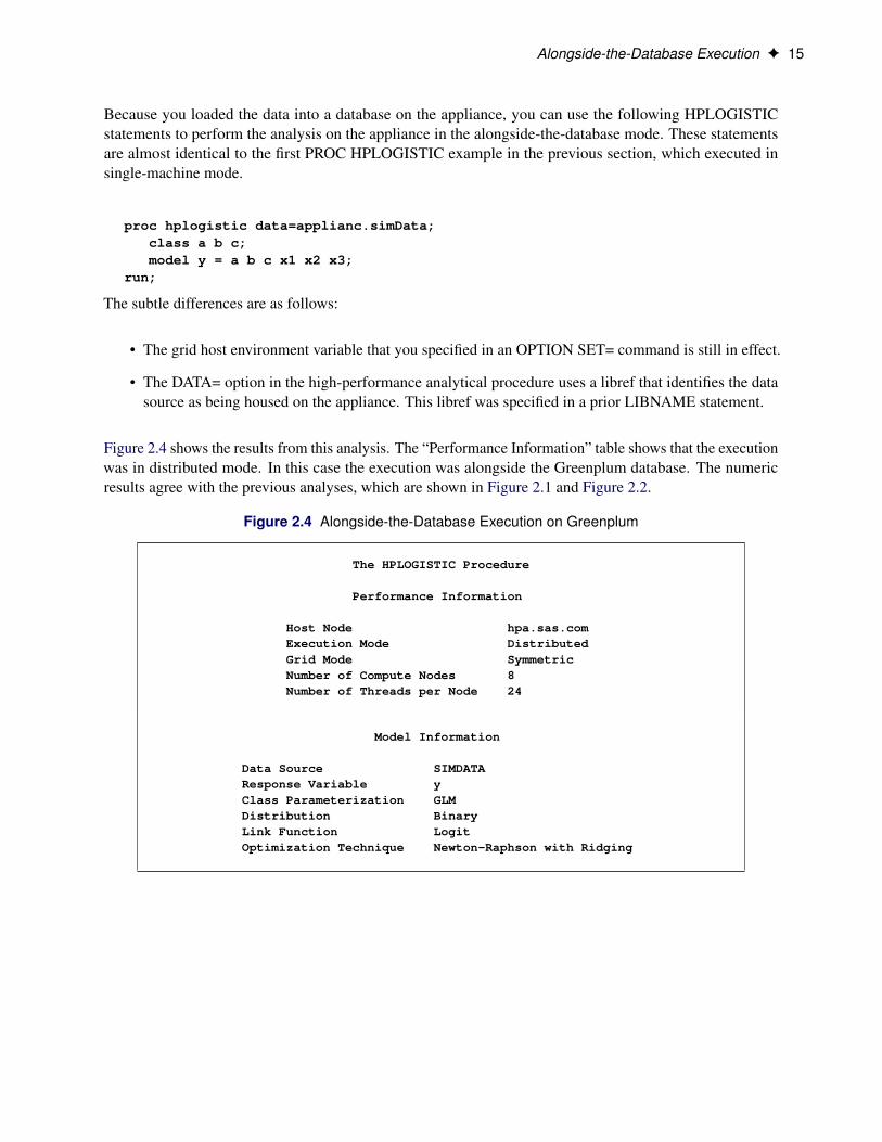
Figure 2.4 shows the results from this analysis. The “Performance Information” table shows that the executionwas in distributed mode. In this case the execution was alongside the Greenplum database. The numericresults agree with the previous analyses, which are shown in Figure 2.1 and Figure 2.2.
Figure 2.4 Alongside-the-Database Execution on Greenplum
The HPLOGISTIC Procedure
Performance Information
Host Node hpa.sas.comExecution Mode DistributedGrid Mode SymmetricNumber of Compute Nodes 8Number of Threads per Node 24
Model Information
Data Source SIMDATAResponse Variable yClass Parameterization GLMDistribution BinaryLink Function LogitOptimization Technique Newton-Raphson with Ridging
16 F Chapter 2: Shared Concepts and Topics
Figure 2.4 continued
Parameter Estimates
StandardParameter Estimate Error DF t Value Pr > |t|
Intercept 5.7011 0.2539 Infty 22.45 <.0001a 0 -0.01020 0.06627 Infty -0.15 0.8777a 1 0 . . . .b 0 0.7124 0.06558 Infty 10.86 <.0001b 1 0 . . . .c 0 0.8036 0.06456 Infty 12.45 <.0001c 1 0 . . . .x1 0.01975 0.000614 Infty 32.15 <.0001x2 -0.04728 0.003098 Infty -15.26 <.0001x3 -0.1017 0.009470 Infty -10.74 <.0001
When high-performance analytical procedures execute symmetrically alongside the database, any nonzerospecification of the NODES= option in the PERFORMANCE statement is ignored. If the data are readalongside the database, the number of compute nodes is determined by the layout of the database and cannotbe modified. In this example, the appliance contains 16 nodes. (See the “Performance Information” table.)
However, when high-performance analytical procedures execute asymmetrically alongside the database, thenumber of compute nodes that you specify in the PERFORMANCE statement can differ from the number ofnodes across which the data are partitioned. For an example, see the section “Running High-PerformanceAnalytical Procedures in Asymmetric Mode” on page 19.
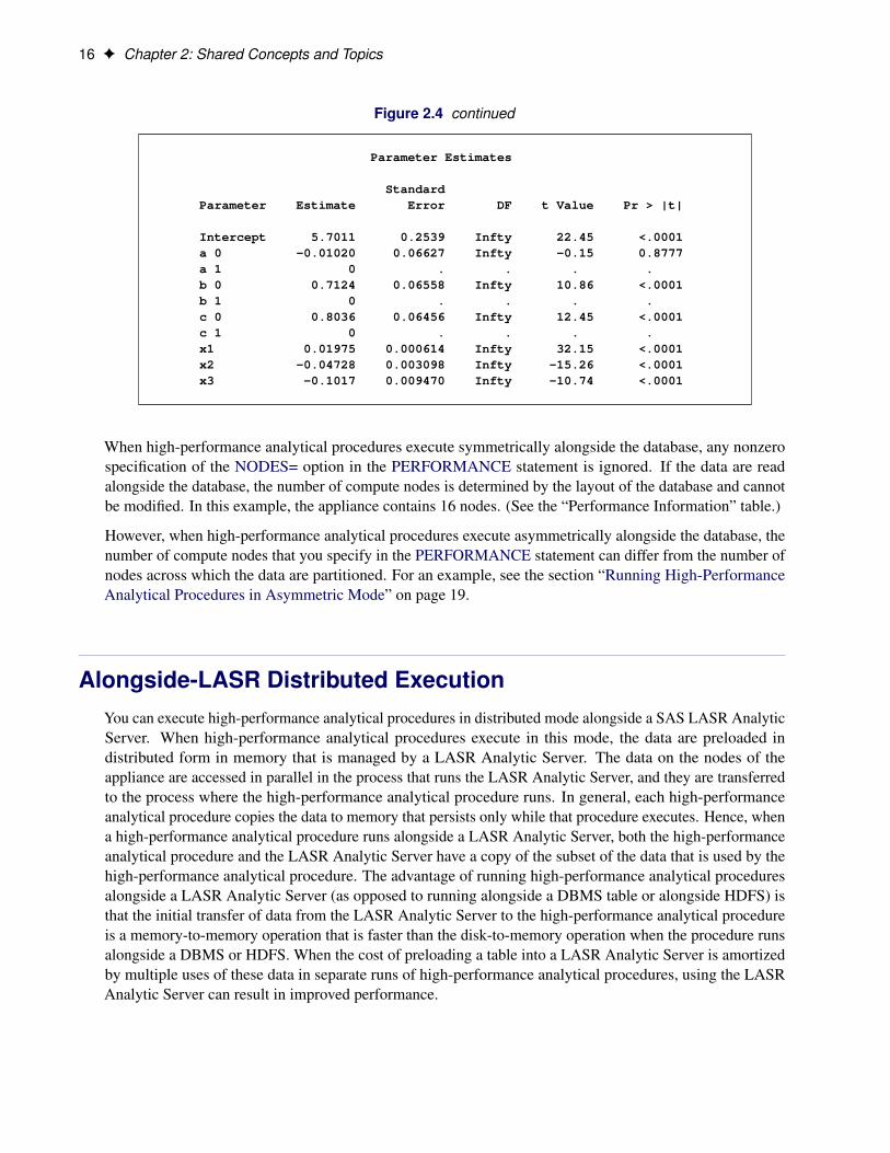
Alongside-LASR Distributed ExecutionYou can execute high-performance analytical procedures in distributed mode alongside a SAS LASR AnalyticServer. When high-performance analytical procedures execute in this mode, the data are preloaded indistributed form in memory that is managed by a LASR Analytic Server. The data on the nodes of theappliance are accessed in parallel in the process that runs the LASR Analytic Server, and they are transferredto the process where the high-performance analytical procedure runs. In general, each high-performanceanalytical procedure copies the data to memory that persists only while that procedure executes. Hence, whena high-performance analytical procedure runs alongside a LASR Analytic Server, both the high-performanceanalytical procedure and the LASR Analytic Server have a copy of the subset of the data that is used by thehigh-performance analytical procedure. The advantage of running high-performance analytical proceduresalongside a LASR Analytic Server (as opposed to running alongside a DBMS table or alongside HDFS) isthat the initial transfer of data from the LASR Analytic Server to the high-performance analytical procedureis a memory-to-memory operation that is faster than the disk-to-memory operation when the procedure runsalongside a DBMS or HDFS. When the cost of preloading a table into a LASR Analytic Server is amortizedby multiple uses of these data in separate runs of high-performance analytical procedures, using the LASRAnalytic Server can result in improved performance.
Starting a SAS LASR Analytic Server Instance F 17
Running High-Performance Analytical Procedures Alongsidea SAS LASR Analytic Server in Distributed ModeThis section provides an example of steps that you can use to start and load data into a SAS LASR AnalyticServer instance and then run high-performance analytical procedures alongside this LASR Analytic Serverinstance.
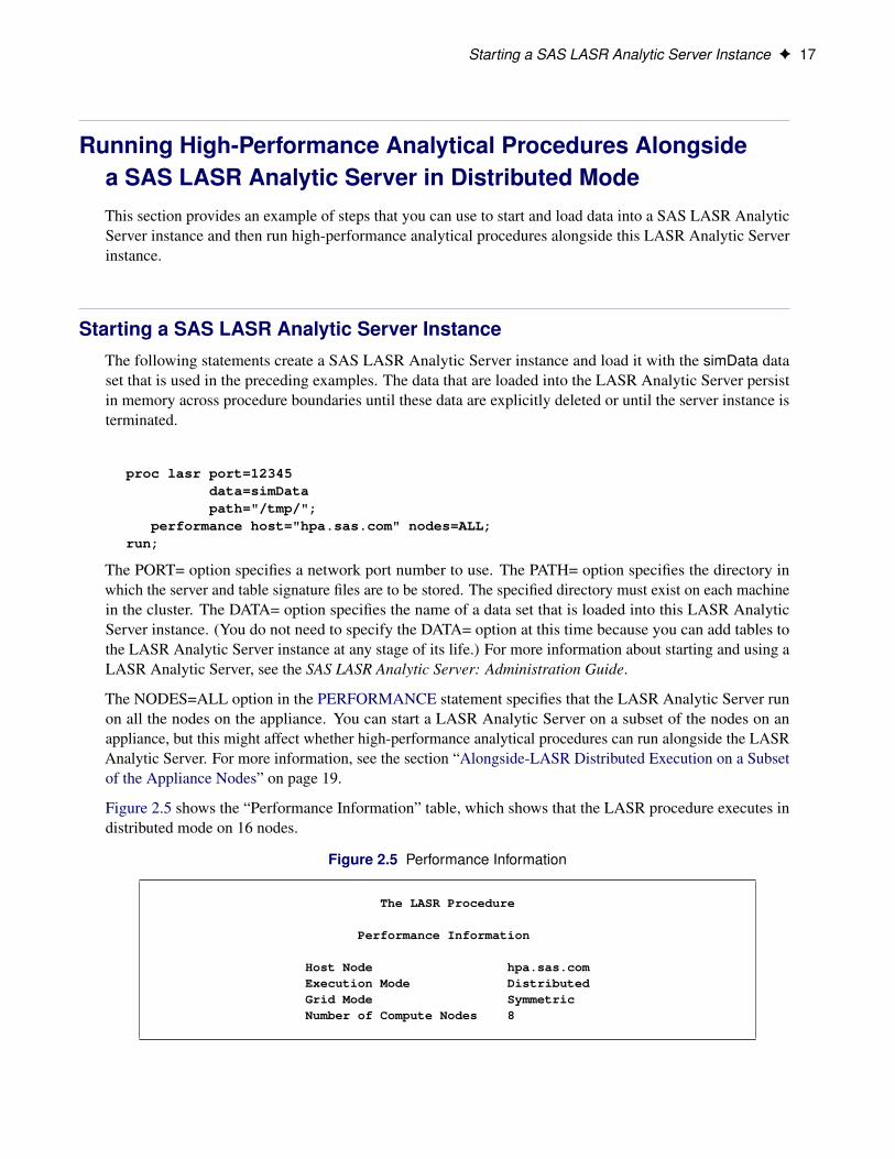
Starting a SAS LASR Analytic Server InstanceThe following statements create a SAS LASR Analytic Server instance and load it with the simData dataset that is used in the preceding examples. The data that are loaded into the LASR Analytic Server persistin memory across procedure boundaries until these data are explicitly deleted or until the server instance isterminated.
proc lasr port=12345data=simDatapath="/tmp/";
performance host="hpa.sas.com" nodes=ALL;run;
The PORT= option specifies a network port number to use. The PATH= option specifies the directory inwhich the server and table signature files are to be stored. The specified directory must exist on each machinein the cluster. The DATA= option specifies the name of a data set that is loaded into this LASR AnalyticServer instance. (You do not need to specify the DATA= option at this time because you can add tables tothe LASR Analytic Server instance at any stage of its life.) For more information about starting and using aLASR Analytic Server, see the SAS LASR Analytic Server: Administration Guide.
The NODES=ALL option in the PERFORMANCE statement specifies that the LASR Analytic Server runon all the nodes on the appliance. You can start a LASR Analytic Server on a subset of the nodes on anappliance, but this might affect whether high-performance analytical procedures can run alongside the LASRAnalytic Server. For more information, see the section “Alongside-LASR Distributed Execution on a Subsetof the Appliance Nodes” on page 19.
Figure 2.5 shows the “Performance Information” table, which shows that the LASR procedure executes indistributed mode on 16 nodes.
Figure 2.5 Performance Information
The LASR Procedure
Performance Information
Host Node hpa.sas.comExecution Mode DistributedGrid Mode SymmetricNumber of Compute Nodes 8
18 F Chapter 2: Shared Concepts and Topics
Associating a SAS Libref with the SAS LASR Analytic Server InstanceThe following statements use a LIBNAME statement that associates a SAS libref (named MyLasr) withtables on the server instance as follows:
libname MyLasr sasiola port=12345;
The SASIOLA option requests that the MyLasr libref use the SASIOLA engine, and the PORT= valueassociates this libref with the appropriate server instance. For more information about creating a libref thatuses the SASIOLA engine, see the SAS LASR Analytic Server: Administration Guide.
Running a High-Performance Analytical Procedure Alongside the SASLASR Analytic Server InstanceYou can use the MyLasr libref to specify the input data for high-performance analytical procedures. You canalso create output data sets in the SAS LASR Analytic Server instance by using this libref to request that theoutput data set be held in memory by the server instance as follows:
proc hplogistic data=MyLasr.simData;class a b c;model y = a b c x1 x2 x3;output out=MyLasr.simulateScores pred=PredictedProbabliity;
run;
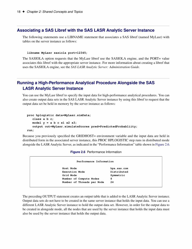
Because you previously specified the GRIDHOST= environment variable and the input data are held indistributed form in the associated server instance, this PROC HPLOGISTIC step runs in distributed modealongside the LASR Analytic Server, as indicated in the “Performance Information” table shown in Figure 2.6.
Figure 2.6 Performance Information
Performance Information
Host Node hpa.sas.comExecution Mode DistributedGrid Mode SymmetricNumber of Compute Nodes 8Number of Threads per Node 24
The preceding OUTPUT statement creates an output table that is added to the LASR Analytic Server instance.Output data sets do not have to be created in the same server instance that holds the input data. You can use adifferent LASR Analytic Server instance to hold the output data set. However, in order for the output data tobe created in alongside mode, all the nodes that are used by the server instance that holds the input data mustalso be used by the server instance that holds the output data.

Terminating a SAS LASR Analytic Server Instance F 19
Terminating a SAS LASR Analytic Server InstanceYou can continue to run high-performance analytical procedures and add and delete tables from the SASLASR Analytic Server instance until you terminate the server instance as follows:
proc lasr term port=12345;run;
Alongside-LASR Distributed Execution on a Subset of theAppliance NodesWhen you run PROC LASR to start a SAS LASR Analytic Server, you can specify the NODES= option in aPERFORMANCE statement to control how many nodes the LASR Analytic Server executes on. Similarly,a high-performance analytical procedure can execute on a subset of the nodes either because you specifythe NODES= option in a PERFORMANCE statement or because you run alongside a DBMS or HDFSwith an input data set that is distributed on a subset of the nodes on an appliance. In such situations, if ahigh-performance analytical procedure uses nodes on which the LASR Analytic Server is not running, thenrunning alongside LASR is not supported. You can avoid this issue by specifying the NODES=ALL in thePERFORMANCE statement when you use PROC LASR to start the LASR Analytic Server.
Running High-Performance Analytical Procedures inAsymmetric ModeThis section provides examples of how you can run high-performance analytical procedures in asymmetricmode. It also includes examples that run in symmetric mode to highlight differences between the modes.For a description of asymmetric mode, see the section “Symmetric and Asymmetric Distributed Modes” onpage 7.
Asymmetric mode is commonly used when the data appliance and the computing appliance are distinctappliances. In order to be able to use an appliance as a data provider for high-performance analyticalprocedures that run in asymmetric mode on another appliance, it is not necessary that SAS High-PerformanceStatistics be installed on the data appliance. However, it is essential that a SAS Embedded Process be installedon the data appliance and that SAS High-Performance Statistics be installed on the computing appliance.
The following examples use a 24-node data appliance named “data_appliance.sas.com,” which houses aTeradata DBMS and has a SAS Embedded Process installed. Because SAS High-Performance Statisticsis also installed on this appliance, it can be used to run high-performance analytical procedures in bothsymmetric and asymmetric modes.
20 F Chapter 2: Shared Concepts and Topics
The following statements load the simData data set of the preceding sections onto the data appliance:
libname dataLib teradataserver ="tera2650"user =XXXXXXpassword=YYYYYdatabase=mydb;
data dataLib.simData;set simData;
run;
NOTE: You can provision the appliance with data even if SAS High-Performance Statistics software is notinstalled on the appliance.
The following subsections show how you can run the HPLOGISTIC procedure symmetrically and asymmet-rically on a single data appliance and asymmetrically on distinct data and computing appliances.
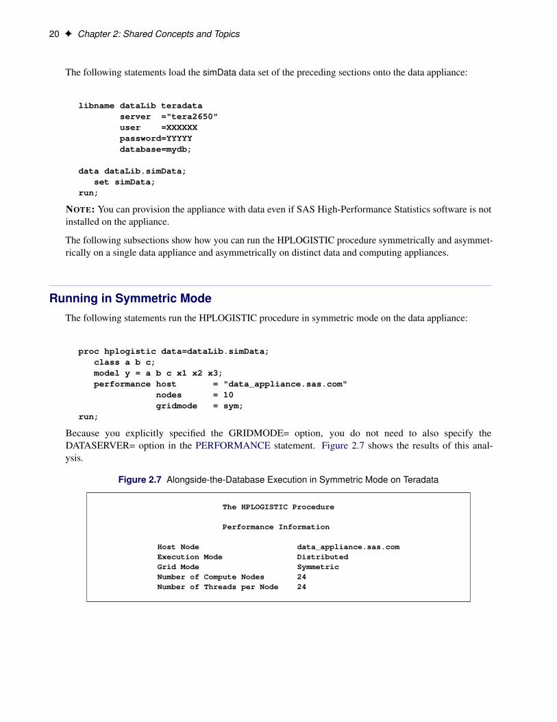
Running in Symmetric ModeThe following statements run the HPLOGISTIC procedure in symmetric mode on the data appliance:
proc hplogistic data=dataLib.simData;class a b c;model y = a b c x1 x2 x3;performance host = "data_appliance.sas.com"
nodes = 10gridmode = sym;
run;
Because you explicitly specified the GRIDMODE= option, you do not need to also specify theDATASERVER= option in the PERFORMANCE statement. Figure 2.7 shows the results of this anal-ysis.
Figure 2.7 Alongside-the-Database Execution in Symmetric Mode on Teradata
The HPLOGISTIC Procedure
Performance Information
Host Node data_appliance.sas.comExecution Mode DistributedGrid Mode SymmetricNumber of Compute Nodes 24Number of Threads per Node 24
Running in Asymmetric Mode on One Appliance F 21
Figure 2.7 continued
Model Information
Data Source simDataResponse Variable yClass Parameterization GLMDistribution BinaryLink Function LogitOptimization Technique Newton-Raphson with Ridging
Parameter Estimates
StandardParameter Estimate Error DF t Value Pr > |t|
Intercept 5.7011 0.2539 Infty 22.45 <.0001a 0 -0.01020 0.06627 Infty -0.15 0.8777a 1 0 . . . .b 0 0.7124 0.06558 Infty 10.86 <.0001b 1 0 . . . .c 0 0.8036 0.06456 Infty 12.45 <.0001c 1 0 . . . .x1 0.01975 0.000614 Infty 32.15 <.0001x2 -0.04728 0.003098 Infty -15.26 <.0001x3 -0.1017 0.009470 Infty -10.74 <.0001
The “Performance Information” table shows that the execution occurs in symmetric mode on the 24 nodes ofthe data appliance. In this case, the NODES=10 option in the PERFORMANCE statement is ignored becausethe number of nodes that are used is determined by the number of nodes across which the data are distributed,as indicated in the following warning message in the SAS log:
WARNING: The NODES=10 option in the PERFORMANCE statement is ignored becauseyou are running alongside the distributed data sourceDATALIB.simData.DATA. The number of compute nodes is determined by theconfiguration of the distributed DBMS.
Running in Asymmetric Mode on One ApplianceYou can switch to running the HPLOGISTIC procedure in asymmetric mode by specifying the GRID-MODE=ASYM option in the PERFORMANCE statement as follows:
proc hplogistic data=dataLib.simData;class a b c;model y = a b c x1 x2 x3;performance host = "data_appliance.sas.com"
nodes = 10gridmode = asym;
run;
22 F Chapter 2: Shared Concepts and Topics
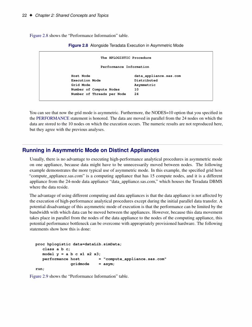
Figure 2.8 shows the “Performance Information” table.
Figure 2.8 Alongside Teradata Execution in Asymmetric Mode
The HPLOGISTIC Procedure
Performance Information
Host Node data_appliance.sas.comExecution Mode DistributedGrid Mode AsymmetricNumber of Compute Nodes 10Number of Threads per Node 24
You can see that now the grid mode is asymmetric. Furthermore, the NODES=10 option that you specified inthe PERFORMANCE statement is honored. The data are moved in parallel from the 24 nodes on which thedata are stored to the 10 nodes on which the execution occurs. The numeric results are not reproduced here,but they agree with the previous analyses.
Running in Asymmetric Mode on Distinct AppliancesUsually, there is no advantage to executing high-performance analytical procedures in asymmetric modeon one appliance, because data might have to be unnecessarily moved between nodes. The followingexample demonstrates the more typical use of asymmetric mode. In this example, the specified grid host“compute_appliance.sas.com” is a computing appliance that has 15 compute nodes, and it is a differentappliance from the 24-node data appliance “data_appliance.sas.com,” which houses the Teradata DBMSwhere the data reside.
The advantage of using different computing and data appliances is that the data appliance is not affected bythe execution of high-performance analytical procedures except during the initial parallel data transfer. Apotential disadvantage of this asymmetric mode of execution is that the performance can be limited by thebandwidth with which data can be moved between the appliances. However, because this data movementtakes place in parallel from the nodes of the data appliance to the nodes of the computing appliance, thispotential performance bottleneck can be overcome with appropriately provisioned hardware. The followingstatements show how this is done:
proc hplogistic data=dataLib.simData;class a b c;model y = a b c x1 x2 x3;performance host = "compute_appliance.sas.com"
gridmode = asym;run;
Figure 2.9 shows the “Performance Information” table.
Running in Asymmetric Mode on Distinct Appliances F 23
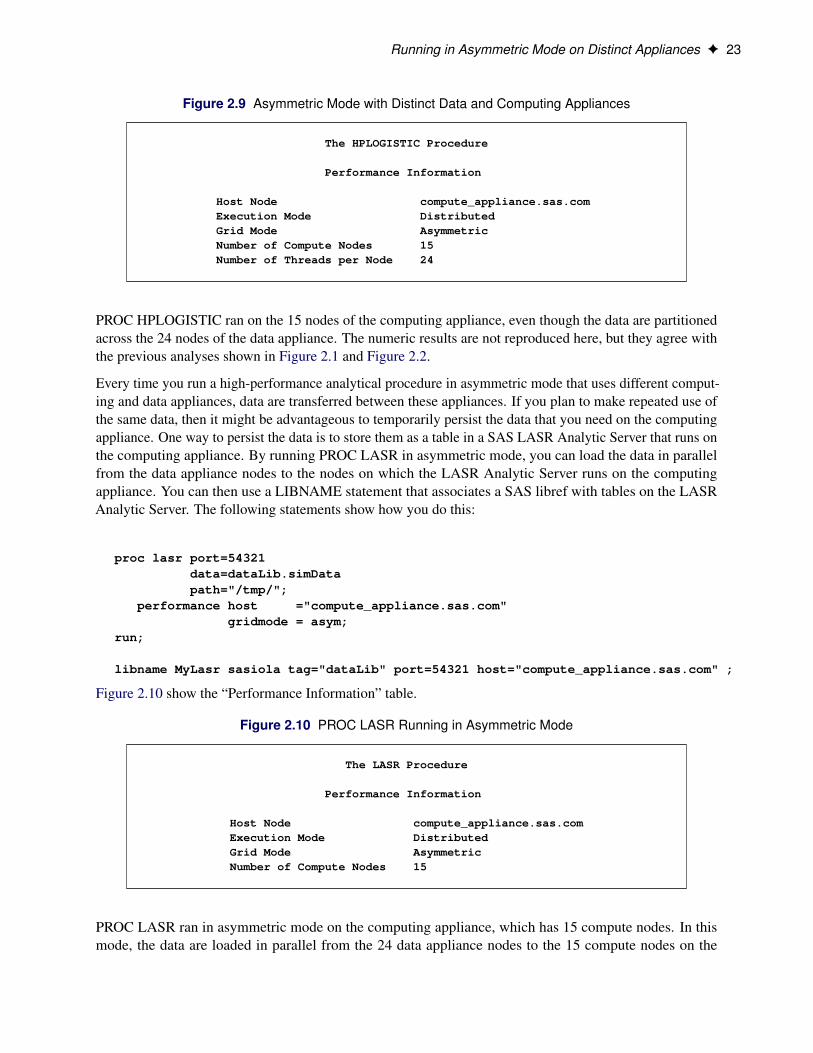
Figure 2.9 Asymmetric Mode with Distinct Data and Computing Appliances
The HPLOGISTIC Procedure
Performance Information
Host Node compute_appliance.sas.comExecution Mode DistributedGrid Mode AsymmetricNumber of Compute Nodes 15Number of Threads per Node 24
PROC HPLOGISTIC ran on the 15 nodes of the computing appliance, even though the data are partitionedacross the 24 nodes of the data appliance. The numeric results are not reproduced here, but they agree withthe previous analyses shown in Figure 2.1 and Figure 2.2.
Every time you run a high-performance analytical procedure in asymmetric mode that uses different comput-ing and data appliances, data are transferred between these appliances. If you plan to make repeated use ofthe same data, then it might be advantageous to temporarily persist the data that you need on the computingappliance. One way to persist the data is to store them as a table in a SAS LASR Analytic Server that runs onthe computing appliance. By running PROC LASR in asymmetric mode, you can load the data in parallelfrom the data appliance nodes to the nodes on which the LASR Analytic Server runs on the computingappliance. You can then use a LIBNAME statement that associates a SAS libref with tables on the LASRAnalytic Server. The following statements show how you do this:
proc lasr port=54321data=dataLib.simDatapath="/tmp/";
performance host ="compute_appliance.sas.com"gridmode = asym;
run;
libname MyLasr sasiola tag="dataLib" port=54321 host="compute_appliance.sas.com" ;
Figure 2.10 show the “Performance Information” table.
Figure 2.10 PROC LASR Running in Asymmetric Mode
The LASR Procedure
Performance Information
Host Node compute_appliance.sas.comExecution Mode DistributedGrid Mode AsymmetricNumber of Compute Nodes 15
PROC LASR ran in asymmetric mode on the computing appliance, which has 15 compute nodes. In thismode, the data are loaded in parallel from the 24 data appliance nodes to the 15 compute nodes on the
24 F Chapter 2: Shared Concepts and Topics
computing appliance. By default, all the nodes on the computing appliance are used. You can use theNODES= option in the PERFORMANCE statement to run the LASR Analytic Server on a subset of thenodes on the computing appliance. If you omit the GRIDMODE=ASYM option from the PERFORMANCEstatement, PROC LASR still runs successfully but much less efficiently. The Teradata access engine transfersthe simData data set to a temporary table on the client, and the High-Performance Analytics infrastructurethen transfers these data from the temporary table on the client to the grid nodes on the computing appliance.
After the data are loaded into a LASR Analytic Server that runs on the computing appliance, you can runhigh-performance analytical procedures alongside this LASR Analytic Server. Because these proceduresrun on the same computing appliance where the LASR Analytic Server is running, it is best to run theseprocedures in symmetric mode, which is the default or can be explicitly specified in the GRIDMODE=SYMoption in the PERFORMANCE statement. The following statements provide an example. The OUTPUTstatement creates an output data set that is held in memory by the LASR Analytic Server. The data appliancehas no role in executing these statements.
proc hplogistic data=MyLasr.simData;class a b c;model y = a b c x1 x2 x3;output out=MyLasr.myOutputData pred=myPred;performance host = "compute_appliance.sas.com";
run;
The following note, which appears in the SAS log, confirms that the output data set is created successfully:
NOTE: The table DATALIB.MYOUTPUTDATA has been added to the LASR Analytic Serverwith port 54321. The Libname is MYLASR.
You can use the dataLib libref that you used to load the data onto the data appliance to create an outputdata set on the data appliance. In order for this output to be directly written in parallel from the nodes ofthe computing appliance to the nodes of the data appliance, you need to run the HPLOGISTIC procedurein asymmetric mode by specifying the GRIDMODE=ASYM option in the PERFORMANCE statement asfollows:
proc hplogistic data=MyLasr.simData;class a b c;model y = a b c x1 x2 x3;output out=dataLib.myOutputData pred=myPred;performance host = "compute_appliance.sas.com"
gridmode = asym;run;
The following note, which appears in the SAS log, confirms that the output data set is created successfully onthe data appliance:
NOTE: The data set DATALIB.myOutputData has 100000 observations and 1 variables.
When you run a high-performance analytical procedure on a computing appliance and either read data fromor write data to a different data appliance, it is important to run the high-performance analytical proceduresin asymmetric mode so that the Read and Write operations take place in parallel without any movement ofdata to and from the SAS client. If you omit running the preceding PROC HPLOGISTIC step in asymmetricmode, then the output data set would be created much less efficiently: the output data would be movedsequentially to a temporary table on the client, after which the Teradata access engine sequentially wouldwrite this table to the data appliance.
Alongside-HDFS Execution F 25
When you no longer need the data in the SAS LASR Analytic Server, you should terminate the server instanceas follows:
proc lasr term port=54321;performance host="compute_appliance.sas.com";
run;
If you configured Hadoop on the computing appliance, then you can create output data tables that are storedin the HDFS on the computing appliance. You can do this by using the SASHDAT engine as described in thesection “Alongside-HDFS Execution” on page 25.
Alongside-HDFS ExecutionRunning high-performance analytical procedures alongside HDFS shares many features with running along-side the database. You can execute high-performance analytical procedures alongside HDFS by using eitherthe SASHDAT engine or the Hadoop engine.
You use the SASHDAT engine to read and write data that are stored in HDFS in a proprietary SASHDATformat. In SASHDAT format, metadata that describe the data in the Hadoop files are included with thedata. This enables you to access files in SASHDAT format without supplying any additional metadata.Additionally, you can also use the SASHDAT engine to read data in CSV (comma-separated value) format,but you need supply metadata that describe the contents of the CSV data. The SASHDAT engine provideshighly optimized access to data in HDFS that are stored in SASHDAT format.
The Hadoop engine reads data that are stored in various formats from HDFS and writes data to HDFS inCSV format. This engine can use metadata that are stored in Hive, which is a data warehouse that suppliesmetadata about data that are stored in Hadoop files. In addition, this engine can use metadata that you createby using the HDMD procedure.
The following subsections provide details about using the SASHDAT and Hadoop engines to executehigh-performance analytical procedures alongside HDFS.
Alongside-HDFS Execution by Using the SASHDAT EngineIf the grid host is a cluster that houses data that have been distributed by using the SASHDAT engine, thenhigh-performance analytical procedures can analyze those data in the alongside-HDFS mode. The proceduresuse the distributed computing environment in which an analytic process is co-located with the nodes of thecluster. Data then pass from HDFS to the analytic process on each node of the cluster.
Before you can run a procedure alongside HDFS, you must distribute the data to the cluster. The followingstatements use the SASHDAT engine to distribute to HDFS the simData data set that was used in the previoustwo sections:
option set=GRIDHOST="hpa.sas.com";
libname hdatLib sashdatpath="/hps";
26 F Chapter 2: Shared Concepts and Topics
data hdatLib.simData (replace = yes) ;set simData;
run;
In this example, the GRIDHOST is a cluster where the SAS Data in HDFS Engine is installed. If a data set thatis named simData already exists in the hps directory in HDFS, it is overwritten because the REPLACE=YESdata set option is specified. For more information about using this LIBNAME statement, see the section“LIBNAME Statement for the SAS Data in HDFS Engine” in the SAS LASR Analytic Server: AdministrationGuide.
The following HPLOGISTIC procedure statements perform the analysis in alongside-HDFS mode. Thesestatements are almost identical to the PROC HPLOGISTIC example in the previous two sections, whichexecuted in single-machine mode and alongside-the-database distributed mode, respectively.
proc hplogistic data=hdatLib.simData;class a b c;model y = a b c x1 x2 x3;
run;
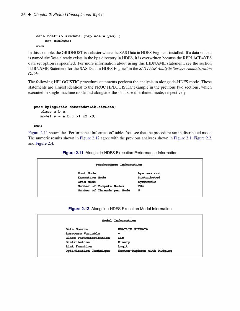
Figure 2.11 shows the “Performance Information” table. You see that the procedure ran in distributed mode.The numeric results shown in Figure 2.12 agree with the previous analyses shown in Figure 2.1, Figure 2.2,and Figure 2.4.
Figure 2.11 Alongside-HDFS Execution Performance Information
Performance Information
Host Node hpa.sas.comExecution Mode DistributedGrid Mode SymmetricNumber of Compute Nodes 206Number of Threads per Node 8
Figure 2.12 Alongside-HDFS Execution Model Information
Model Information
Data Source HDATLIB.SIMDATAResponse Variable yClass Parameterization GLMDistribution BinaryLink Function LogitOptimization Technique Newton-Raphson with Ridging
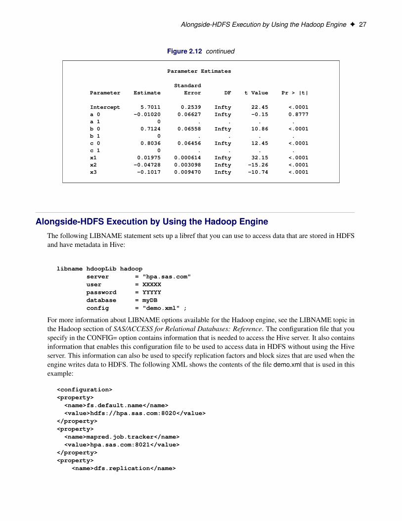
Alongside-HDFS Execution by Using the Hadoop Engine F 27
Figure 2.12 continued
Parameter Estimates
StandardParameter Estimate Error DF t Value Pr > |t|
Intercept 5.7011 0.2539 Infty 22.45 <.0001a 0 -0.01020 0.06627 Infty -0.15 0.8777a 1 0 . . . .b 0 0.7124 0.06558 Infty 10.86 <.0001b 1 0 . . . .c 0 0.8036 0.06456 Infty 12.45 <.0001c 1 0 . . . .x1 0.01975 0.000614 Infty 32.15 <.0001x2 -0.04728 0.003098 Infty -15.26 <.0001x3 -0.1017 0.009470 Infty -10.74 <.0001
Alongside-HDFS Execution by Using the Hadoop EngineThe following LIBNAME statement sets up a libref that you can use to access data that are stored in HDFSand have metadata in Hive:
libname hdoopLib hadoopserver = "hpa.sas.com"user = XXXXXpassword = YYYYYdatabase = myDBconfig = "demo.xml" ;
For more information about LIBNAME options available for the Hadoop engine, see the LIBNAME topic inthe Hadoop section of SAS/ACCESS for Relational Databases: Reference. The configuration file that youspecify in the CONFIG= option contains information that is needed to access the Hive server. It also containsinformation that enables this configuration file to be used to access data in HDFS without using the Hiveserver. This information can also be used to specify replication factors and block sizes that are used when theengine writes data to HDFS. The following XML shows the contents of the file demo.xml that is used in thisexample:
<configuration><property>
<name>fs.default.name</name><value>hdfs://hpa.sas.com:8020</value>
</property><property>
<name>mapred.job.tracker</name><value>hpa.sas.com:8021</value>
</property><property>
<name>dfs.replication</name>

28 F Chapter 2: Shared Concepts and Topics
<value>1</value></property><property>
<name>dfs.block.size</name><value>33554432</value>
</property></configuration>
The following DATA step uses the Hadoop engine to distribute to HDFS the simData data set that was usedin the previous sections. The engine creates metadata for the data set in Hive.
data hdoopLib.simData;set simData;
run;
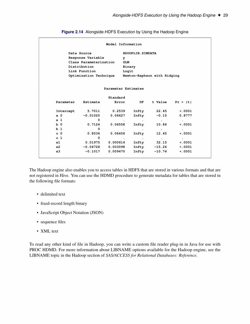
After you have loaded data or if you are accessing preexisting data in HDFS that have metadata in Hive,you can access this data alongside HDFS by using high-performance analytics procedures. The followingHPLOGISTIC procedure statements perform the analysis in alongside-HDFS mode. These statements aresimilar to the PROC HPLOGISTIC example in the previous sections. However, whenever you use theHadoop engine, you must execute the analysis in asymmetric mode to cause the execution to occur alongsideHDFS.
proc hplogistic data=hdoopLib.simData;class a b c;model y = a b c x1 x2 x3;performance host = "compute_appliance.sas.com"
gridmode = asym;run;
Figure 2.13 shows the “Performance Information” table. You see that the procedure ran asymmetrically indistributed mode. The numeric results shown in Figure 2.14 agree with the previous analyses.
Figure 2.13 Alongside-HDFS Execution by Using the Hadoop Engine
The HPLOGISTIC Procedure
Performance Information
Host Node compute_appliance.sas.comExecution Mode DistributedGrid Mode AsymmetricNumber of Compute Nodes 15Number of Threads per Node 24
Alongside-HDFS Execution by Using the Hadoop Engine F 29
Figure 2.14 Alongside-HDFS Execution by Using the Hadoop Engine
Model Information
Data Source HDOOPLIB.SIMDATAResponse Variable yClass Parameterization GLMDistribution BinaryLink Function LogitOptimization Technique Newton-Raphson with Ridging
Parameter Estimates
StandardParameter Estimate Error DF t Value Pr > |t|
Intercept 5.7011 0.2539 Infty 22.45 <.0001a 0 -0.01020 0.06627 Infty -0.15 0.8777a 1 0 . . . .b 0 0.7124 0.06558 Infty 10.86 <.0001b 1 0 . . . .c 0 0.8036 0.06456 Infty 12.45 <.0001c 1 0 . . . .x1 0.01975 0.000614 Infty 32.15 <.0001x2 -0.04728 0.003098 Infty -15.26 <.0001x3 -0.1017 0.009470 Infty -10.74 <.0001
The Hadoop engine also enables you to access tables in HDFS that are stored in various formats and that arenot registered in Hive. You can use the HDMD procedure to generate metadata for tables that are stored inthe following file formats:
• delimited text
• fixed-record length binary
• JavaScript Object Notation (JSON)
• sequence files
• XML text
To read any other kind of file in Hadoop, you can write a custom file reader plug-in in Java for use withPROC HDMD. For more information about LIBNAME options available for the Hadoop engine, see theLIBNAME topic in the Hadoop section of SAS/ACCESS for Relational Databases: Reference.
30 F Chapter 2: Shared Concepts and Topics
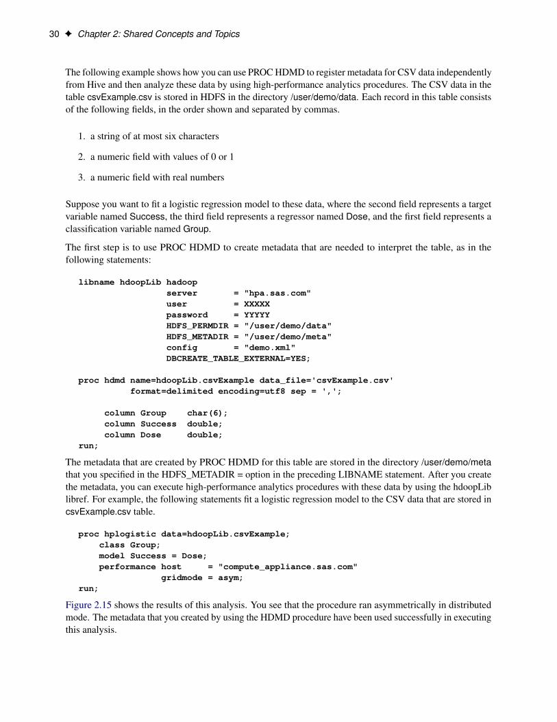
The following example shows how you can use PROC HDMD to register metadata for CSV data independentlyfrom Hive and then analyze these data by using high-performance analytics procedures. The CSV data in thetable csvExample.csv is stored in HDFS in the directory /user/demo/data. Each record in this table consistsof the following fields, in the order shown and separated by commas.
1. a string of at most six characters
2. a numeric field with values of 0 or 1
3. a numeric field with real numbers
Suppose you want to fit a logistic regression model to these data, where the second field represents a targetvariable named Success, the third field represents a regressor named Dose, and the first field represents aclassification variable named Group.
The first step is to use PROC HDMD to create metadata that are needed to interpret the table, as in thefollowing statements:
libname hdoopLib hadoopserver = "hpa.sas.com"user = XXXXXpassword = YYYYYHDFS_PERMDIR = "/user/demo/data"HDFS_METADIR = "/user/demo/meta"config = "demo.xml"DBCREATE_TABLE_EXTERNAL=YES;
proc hdmd name=hdoopLib.csvExample data_file='csvExample.csv'format=delimited encoding=utf8 sep = ',';
column Group char(6);column Success double;column Dose double;
run;
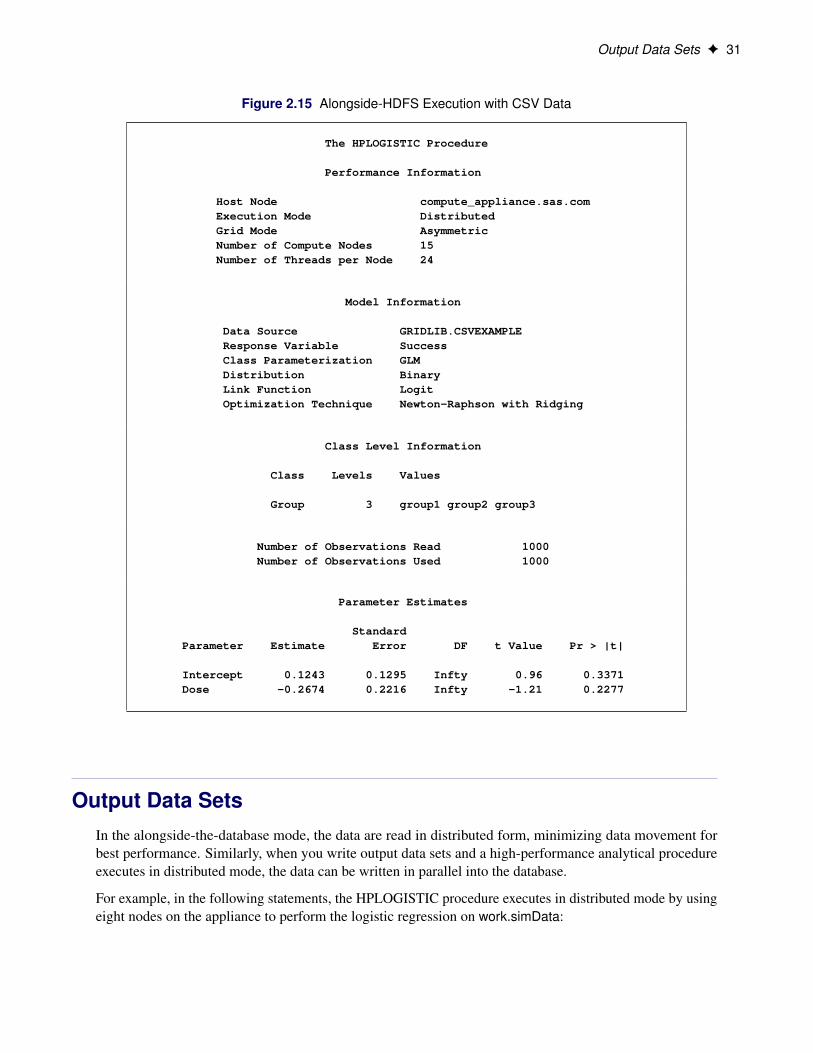
The metadata that are created by PROC HDMD for this table are stored in the directory /user/demo/metathat you specified in the HDFS_METADIR = option in the preceding LIBNAME statement. After you createthe metadata, you can execute high-performance analytics procedures with these data by using the hdoopLiblibref. For example, the following statements fit a logistic regression model to the CSV data that are stored incsvExample.csv table.
proc hplogistic data=hdoopLib.csvExample;class Group;model Success = Dose;performance host = "compute_appliance.sas.com"
gridmode = asym;run;
Figure 2.15 shows the results of this analysis. You see that the procedure ran asymmetrically in distributedmode. The metadata that you created by using the HDMD procedure have been used successfully in executingthis analysis.
Output Data Sets F 31
Figure 2.15 Alongside-HDFS Execution with CSV Data
The HPLOGISTIC Procedure
Performance Information
Host Node compute_appliance.sas.comExecution Mode DistributedGrid Mode AsymmetricNumber of Compute Nodes 15Number of Threads per Node 24
Model Information
Data Source GRIDLIB.CSVEXAMPLEResponse Variable SuccessClass Parameterization GLMDistribution BinaryLink Function LogitOptimization Technique Newton-Raphson with Ridging
Class Level Information
Class Levels Values
Group 3 group1 group2 group3
Number of Observations Read 1000Number of Observations Used 1000
Parameter Estimates
StandardParameter Estimate Error DF t Value Pr > |t|
Intercept 0.1243 0.1295 Infty 0.96 0.3371Dose -0.2674 0.2216 Infty -1.21 0.2277
Output Data SetsIn the alongside-the-database mode, the data are read in distributed form, minimizing data movement forbest performance. Similarly, when you write output data sets and a high-performance analytical procedureexecutes in distributed mode, the data can be written in parallel into the database.
For example, in the following statements, the HPLOGISTIC procedure executes in distributed mode by usingeight nodes on the appliance to perform the logistic regression on work.simData:
32 F Chapter 2: Shared Concepts and Topics
proc hplogistic data=simData;class a b c;model y = a b c x1 x2 x3;id a;output out=applianc.simData_out pred=p;performance host="hpa.sas.com" nodes=8;
run;
The output data set applianc.simData_out is written in parallel into the database. Although the data are fedon eight nodes, the database might distribute the data on more nodes.
When a high-performance analytical procedure executes in single-machine mode, all output objects arecreated on the client. If the libref of the output data sets points to the appliance, the data are transferred to thedatabase on the appliance. This can lead to considerable performance degradation compared to execution indistributed mode.
Many procedures in SAS software add the variables from the input data set when an observationwise outputdata set is created. The assumption of high-performance analytical procedures is that the input data sets canbe large and contain many variables. For performance reasons, the output data set contains the following:
• variables that are explicitly created by the statement
• variables that are listed in the ID statement
• distribution keys or hash keys that are transferred from the input data set
Including this information enables you to add to the output data set information necessary for subsequentSQL joins without copying the entire input data set to the output data set.
Working with FormatsYou can use SAS formats and user-defined formats with high-performance analytical procedures as you canwith other procedures in the SAS System. However, because the analytic work is carried out in a distributedenvironment and might depend on the formatted values of variables, some special handling can improve theefficiency of work with formats.
High-performance analytical procedures examine the variables that are used in an analysis for association withuser-defined formats. Any user-defined formats that are found by a procedure are transmitted automaticallyto the appliance. If you are running multiple high-performance analytical procedures in a SAS session andthe analysis variables depend on user-defined formats, you can preprocess the formats. This step involvesgenerating an XML stream (a file) of the formats and passing the stream to the high-performance analyticalprocedures.
Working with Formats F 33
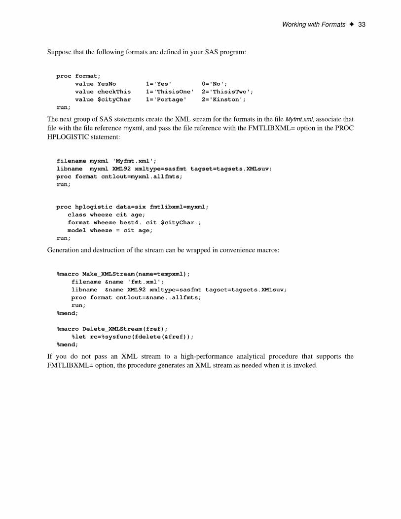
Suppose that the following formats are defined in your SAS program:
proc format;value YesNo 1='Yes' 0='No';value checkThis 1='ThisisOne' 2='ThisisTwo';value $cityChar 1='Portage' 2='Kinston';
run;
The next group of SAS statements create the XML stream for the formats in the file Myfmt.xml, associate thatfile with the file reference myxml, and pass the file reference with the FMTLIBXML= option in the PROCHPLOGISTIC statement:
filename myxml 'Myfmt.xml';libname myxml XML92 xmltype=sasfmt tagset=tagsets.XMLsuv;proc format cntlout=myxml.allfmts;run;
proc hplogistic data=six fmtlibxml=myxml;class wheeze cit age;format wheeze best4. cit $cityChar.;model wheeze = cit age;
run;
Generation and destruction of the stream can be wrapped in convenience macros:
%macro Make_XMLStream(name=tempxml);filename &name 'fmt.xml';libname &name XML92 xmltype=sasfmt tagset=tagsets.XMLsuv;proc format cntlout=&name..allfmts;run;
%mend;
%macro Delete_XMLStream(fref);%let rc=%sysfunc(fdelete(&fref));
%mend;
If you do not pass an XML stream to a high-performance analytical procedure that supports theFMTLIBXML= option, the procedure generates an XML stream as needed when it is invoked.
34 F Chapter 2: Shared Concepts and Topics
PERFORMANCE StatementPERFORMANCE < performance-options > ;
The PERFORMANCE statement defines performance parameters for multithreaded and distributed comput-ing, passes variables that describe the distributed computing environment, and requests detailed results aboutthe performance characteristics of a high-performance analytical procedure.
You can also use the PERFORMANCE statement to control whether a high-performance analytical procedureexecutes in single-machine or distributed mode.
You can specify the following performance-options in the PERFORMANCE statement:
COMMIT=nrequests that the high-performance analytical procedure write periodic updates to the SAS log whenobservations are sent from the client to the appliance for distributed processing.
High-performance analytical procedures do not have to use input data that are stored on the appliance.You can perform distributed computations regardless of the origin or format of the input data, providedthat the data are in a format that can be read by the SAS System (for example, because a SAS/ACCESSengine is available).
In the following example, the HPREG procedure performs LASSO variable selection where the inputdata set is stored on the client:
proc hpreg data=work.one;model y = x1-x500;selection method=lasso;performance nodes=10 host='mydca' commit=10000;
run;
In order to perform the work as requested using 10 nodes on the appliance, the data set Work.Oneneeds to be distributed to the appliance.
High-performance analytical procedures send the data in blocks to the appliance. Whenever the numberof observations sent exceeds an integer multiple of the COMMIT= size, a SAS log message is produced.The message indicates the actual number of observations distributed, and not an integer multiple of theCOMMIT= size.
DATASERVER=“name”specifies the name of the server on Teradata systems as defined through the hosts file and as used inthe LIBNAME statement for Teradata. For example, assume that the hosts file defines the server forTeradata as follows:
myservercop1 33.44.55.66
Then a LIBNAME specification would be as follows:

PERFORMANCE Statement F 35
libname TDLib teradata server=myserver user= password= database= ;
A PERFORMANCE statement to induce running alongside the Teradata server would specify thefollowing:
performance dataserver="myserver";
The DATASERVER= option is not required if you specify the GRIDMODE=option in the PERFOR-MANCE statement or if you set the GRIDMODE environment variable.
Specifying the DATASERVER= option overrides the GRIDDATASERVER environment variable.
DETAILSrequests a table that shows a timing breakdown of the procedure steps.
GRIDHOST=“name”HOST=“name”
specifies the name of the appliance host in single or double quotation marks. If this option is specified,it overrides the value of the GRIDHOST environment variable.
GRIDMODE=SYM | ASYMMODE=SYM | ASYM
specifies whether the high-performance analytical procedure runs in symmetric (SYM) mode orasymmetric (ASYM) mode. The default is GRIDMODE=SYM. For more information about thesemodes, see the section “Symmetric and Asymmetric Distributed Modes” on page 7.
If this option is specified, it overrides the GRIDMODE environment variable.
GRIDTIMEOUT=sTIMEOUT=s
specifies the time-out in seconds for a high-performance analytical procedure to wait for a connectionto the appliance and establish a connection back to the client. The default is 120 seconds. If jobsare submitted to the appliance through workload management tools that might suspend access to theappliance for a longer period, you might want to increase the time-out value.
INSTALL=“name”INSTALLLOC=“name”
specifies the directory in which the shared libraries for the high-performance analytical procedureare installed on the appliance. Specifying the INSTALL= option overrides the GRIDINSTALLLOCenvironment variable.
LASRSERVER=“path”LASR=“path”
specifies the fully qualified path to the description file of a SAS LASR Analytic Server instance. Ifthe input data set is held in memory by this LASR Analytic Server instance, then the procedure runsalongside LASR. This option is not needed to run alongside LASR if the DATA= specification of theinput data uses a libref that is associated with a LASR Analytic Server instance. For more information,see the section “Alongside-LASR Distributed Execution” on page 16 and the SAS LASR AnalyticServer: Administration Guide.
36 F Chapter 2: Shared Concepts and Topics
NODES=ALL | n
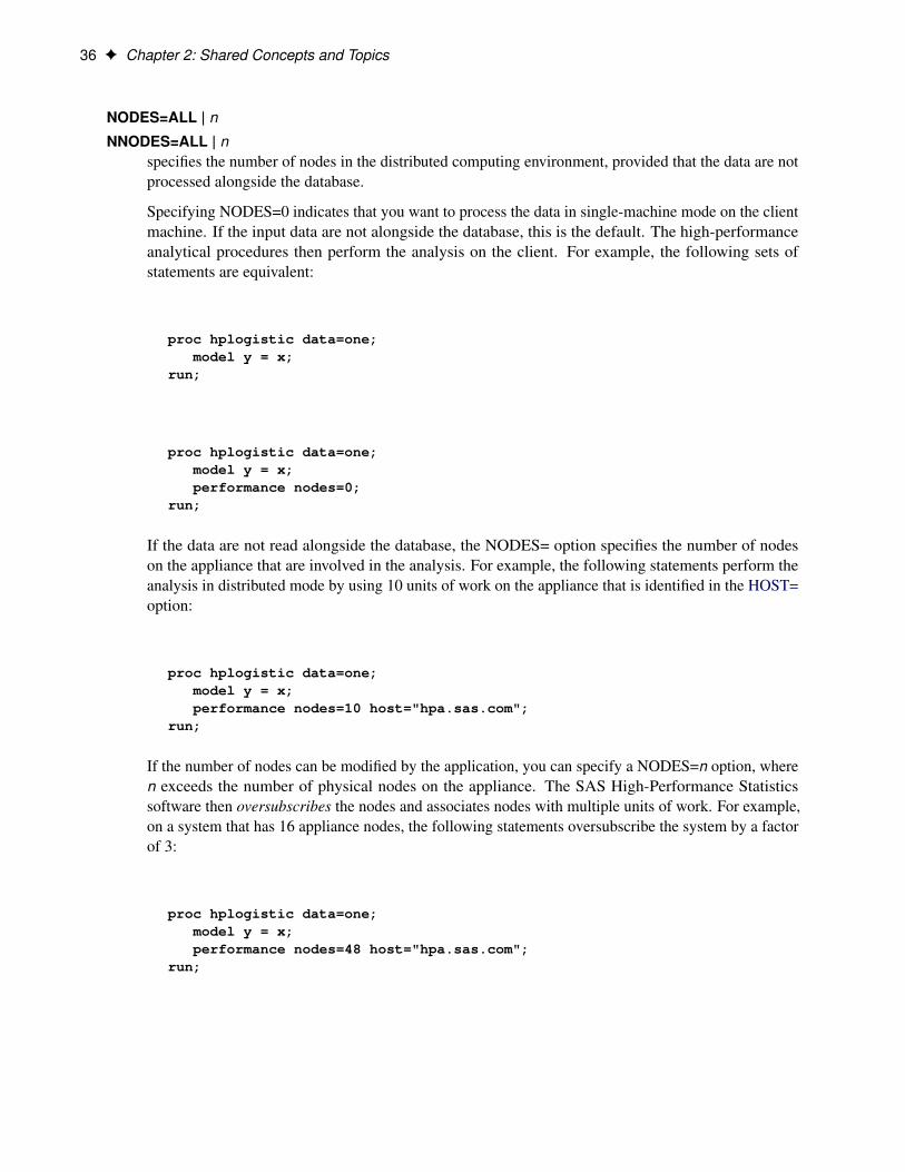
NNODES=ALL | nspecifies the number of nodes in the distributed computing environment, provided that the data are notprocessed alongside the database.
Specifying NODES=0 indicates that you want to process the data in single-machine mode on the clientmachine. If the input data are not alongside the database, this is the default. The high-performanceanalytical procedures then perform the analysis on the client. For example, the following sets ofstatements are equivalent:
proc hplogistic data=one;model y = x;
run;
proc hplogistic data=one;model y = x;performance nodes=0;
run;
If the data are not read alongside the database, the NODES= option specifies the number of nodeson the appliance that are involved in the analysis. For example, the following statements perform theanalysis in distributed mode by using 10 units of work on the appliance that is identified in the HOST=option:
proc hplogistic data=one;model y = x;performance nodes=10 host="hpa.sas.com";
run;
If the number of nodes can be modified by the application, you can specify a NODES=n option, wheren exceeds the number of physical nodes on the appliance. The SAS High-Performance Statisticssoftware then oversubscribes the nodes and associates nodes with multiple units of work. For example,on a system that has 16 appliance nodes, the following statements oversubscribe the system by a factorof 3:
proc hplogistic data=one;model y = x;performance nodes=48 host="hpa.sas.com";
run;
PERFORMANCE Statement F 37
Usually, it is not advisable to oversubscribe the system because the analytic code is optimized fora certain level of multithreading on the nodes that depends on the CPU count. You can specifyNODES=ALL if you want to use all available nodes on the appliance without oversubscribing thesystem.
If the data are read alongside the distributed database on the appliance, specifying a nonzero valuefor the NODES= option has no effect. The number of units of work in the distributed computingenvironment is then determined by the distribution of the data and cannot be altered. For example, ifyou are running alongside an appliance with 24 nodes, the NODES= option in the following statementsis ignored:
libname GPLib greenplm server=gpdca user=XXX password=YYYdatabase=ZZZ;
proc hplogistic data=gplib.one;model y = x;performance nodes=10 host="hpa.sas.com";
run;
NTHREADS=n
THREADS=nspecifies the number of threads for analytic computations and overrides the SAS system optionTHREADS | NOTHREADS. If you do not specify the NTHREADS= option, the number of threads isdetermined based on the number of CPUs on the host on which the analytic computations execute. Thealgorithm by which a CPU count is converted to a thread count is specific to the high-performanceanalytical procedure. Most procedures create one thread per CPU for the analytic computations.
By default, high-performance analytical procedures execute in multiple concurrent threads unlessmultithreading has been turned off by the NOTHREADS system option or you force single-threadedexecution by specifying NTHREADS=1. The largest number that can be specified for n is 256.Individual high-performance analytical procedures can impose more stringent limits if called for byalgorithmic considerations.
NOTE: The SAS system options THREADS | NOTHREADS apply to the client machine on which theSAS high-performance analytical procedures execute. They do not apply to the compute nodes in adistributed environment.

38
Chapter 3
Shared Statistical Concepts
ContentsCommon Features of SAS High-Performance Statistical Procedures . . . . . . . . . . . . . 40Syntax Common to SAS High-Performance Statistical Procedures . . . . . . . . . . . . . . 40
CLASS Statement . . . . . . . . . . . . . . . . . . . . . . . . . . . . . . . . . . . . 40FREQ Statement . . . . . . . . . . . . . . . . . . . . . . . . . . . . . . . . . . . . . 44ID Statement . . . . . . . . . . . . . . . . . . . . . . . . . . . . . . . . . . . . . . . 44SELECTION Statement . . . . . . . . . . . . . . . . . . . . . . . . . . . . . . . . . 45VAR Statement . . . . . . . . . . . . . . . . . . . . . . . . . . . . . . . . . . . . . . 50WEIGHT Statement . . . . . . . . . . . . . . . . . . . . . . . . . . . . . . . . . . . 50
Levelization of Classification Variables . . . . . . . . . . . . . . . . . . . . . . . . . . . . 50Specification and Parameterization of Model Effects . . . . . . . . . . . . . . . . . . . . . 52
Effect Operators . . . . . . . . . . . . . . . . . . . . . . . . . . . . . . . . . . . . . 53Bar and At Sign Operators . . . . . . . . . . . . . . . . . . . . . . . . . . . 54Colon, Dash, and Double Dash Operators . . . . . . . . . . . . . . . . . . . 55
GLM Parameterization of Classification Variables and Effects . . . . . . . . . . . . . 55Intercept . . . . . . . . . . . . . . . . . . . . . . . . . . . . . . . . . . . . . 56Regression Effects . . . . . . . . . . . . . . . . . . . . . . . . . . . . . . . 56Main Effects . . . . . . . . . . . . . . . . . . . . . . . . . . . . . . . . . . 56Interaction Effects . . . . . . . . . . . . . . . . . . . . . . . . . . . . . . . 57Nested Effects . . . . . . . . . . . . . . . . . . . . . . . . . . . . . . . . . . 58Continuous-Nesting-Class Effects . . . . . . . . . . . . . . . . . . . . . . . 58Continuous-by-Class Effects . . . . . . . . . . . . . . . . . . . . . . . . . . 59General Effects . . . . . . . . . . . . . . . . . . . . . . . . . . . . . . . . . 59
Reference Parameterization . . . . . . . . . . . . . . . . . . . . . . . . . . . . . . . 60Model Selection . . . . . . . . . . . . . . . . . . . . . . . . . . . . . . . . . . . . . . . . . 61
Methods . . . . . . . . . . . . . . . . . . . . . . . . . . . . . . . . . . . . . . . . . 61Full Model Fitted . . . . . . . . . . . . . . . . . . . . . . . . . . . . . . . . 61Forward Selection . . . . . . . . . . . . . . . . . . . . . . . . . . . . . . . 61Backward Elimination . . . . . . . . . . . . . . . . . . . . . . . . . . . . . 63Stepwise Selection . . . . . . . . . . . . . . . . . . . . . . . . . . . . . . . 64Forward-Swap Selection . . . . . . . . . . . . . . . . . . . . . . . . . . . . 66Least Angle Regression . . . . . . . . . . . . . . . . . . . . . . . . . . . . . 67Lasso Selection . . . . . . . . . . . . . . . . . . . . . . . . . . . . . . . . . 67Adaptive Lasso Selection . . . . . . . . . . . . . . . . . . . . . . . . . . . . 68
References . . . . . . . . . . . . . . . . . . . . . . . . . . . . . . . . . . . . . . . . . . . 69
40 F Chapter 3: Shared Statistical Concepts
Common Features of SAS High-Performance StatisticalProceduresSAS high-performance statistical procedures behave in many ways like other procedures in the SAS System.This chapter provides details about and describes common syntax elements that are supported by manyhigh-performance statistical procedures. Any deviation by a high-performance statistical procedure from thecommon syntax is documented in the specific chapter for the procedure.
Syntax Common to SAS High-Performance StatisticalProcedures
CLASS StatementCLASS variable < (options) >: : : < variable < (options) > > < / global-options > ;
The CLASS statement names the classification variables to be used as explanatory variables in the analysis.These variables enter the analysis not through their values, but through levels to which the unique valuesare mapped. For more information about these mappings, see the section “Levelization of ClassificationVariables” on page 50.
If a CLASS statement is specified, it must precede the MODEL statement in high-performance statisticalprocedures that support a MODEL statement.
If the procedure permits a classification variable as a response (dependent variable or target), the responsedoes not need to be specified in the CLASS statement.
You can specify options either as individual variable options or as global-options. You can specify optionsfor each variable by enclosing the options in parentheses after the variable name. You can also specifyglobal-options for the CLASS statement by placing them after a slash (/). Global-options are applied to allthe variables that are specified in the CLASS statement. If you specify more than one CLASS statement,the global-options that are specified in any one CLASS statement apply to all CLASS statements. However,individual CLASS variable options override the global-options.
You can specify the following values for either an option or a global-option:
DESCENDING
DESCreverses the sort order of the classification variable. If both the DESCENDING and ORDER= optionsare specified, high-performance statistical procedures order the categories according to the ORDER=option and then reverse that order.
CLASS Statement F 41
ORDER=DATA | FORMATTED | INTERNAL
ORDER=FREQ | FREQDATA | FREQFORMATTED | FREQINTERNALspecifies the sort order for the levels of classification variables. This ordering determines whichparameters in the model correspond to each level in the data. By default, ORDER=FORMATTED.For ORDER=FORMATTED and ORDER=INTERNAL, the sort order is machine-dependent. WhenORDER=FORMATTED is in effect for numeric variables for which you have supplied no explicitformat, the levels are ordered by their internal values.
The following table shows how high-performance statistical procedures interpret values of the ORDER=option.
Value of ORDER= Levels Sorted By
DATA Order of appearance in the input data setFORMATTED External formatted values, except for numeric
variables that have no explicit format, which aresorted by their unformatted (internal) values
FREQ Descending frequency count (levels that havemore observations come earlier in the order)
FREQDATA Order of descending frequency count, and withincounts by order of appearance in the input data setwhen counts are tied
FREQFORMATTED Order of descending frequency count, and withincounts by formatted value when counts are tied
FREQINTERNAL Order of descending frequency count, and withincounts by unformatted (internal) value whencounts are tied
INTERNAL Unformatted value
For more information about sort order, see the chapter about the SORT procedure in Base SASProcedures Guide and the discussion of BY-group processing in SAS Language Reference: Concepts.
REF=’level’ | keyword
REFERENCE=’level’ | keywordspecifies the reference level that is used when you specify PARAM=REFERENCE. For an individual(but not a global) variable REF= option, you can specify the level of the variable to use as the referencelevel. Specify the formatted value of the variable if a format is assigned. For a REF= option orglobal-option, you can use one of the following keywords. The default is REF=LAST.
FIRST designates the first ordered level as reference.
LAST designates the last ordered level as reference.
If you choose a reference level for any CLASS variable, all variables are parameterized in the referenceparameterization for computational efficiency. In other words, high-performance statistical proceduresapply a single parameterization method to all classification variables.
Suppose that the variable temp has three levels ('hot', 'warm', and 'cold') and that the variablegender has two levels ('M' and 'F'). The following statements fit a logistic regression model:
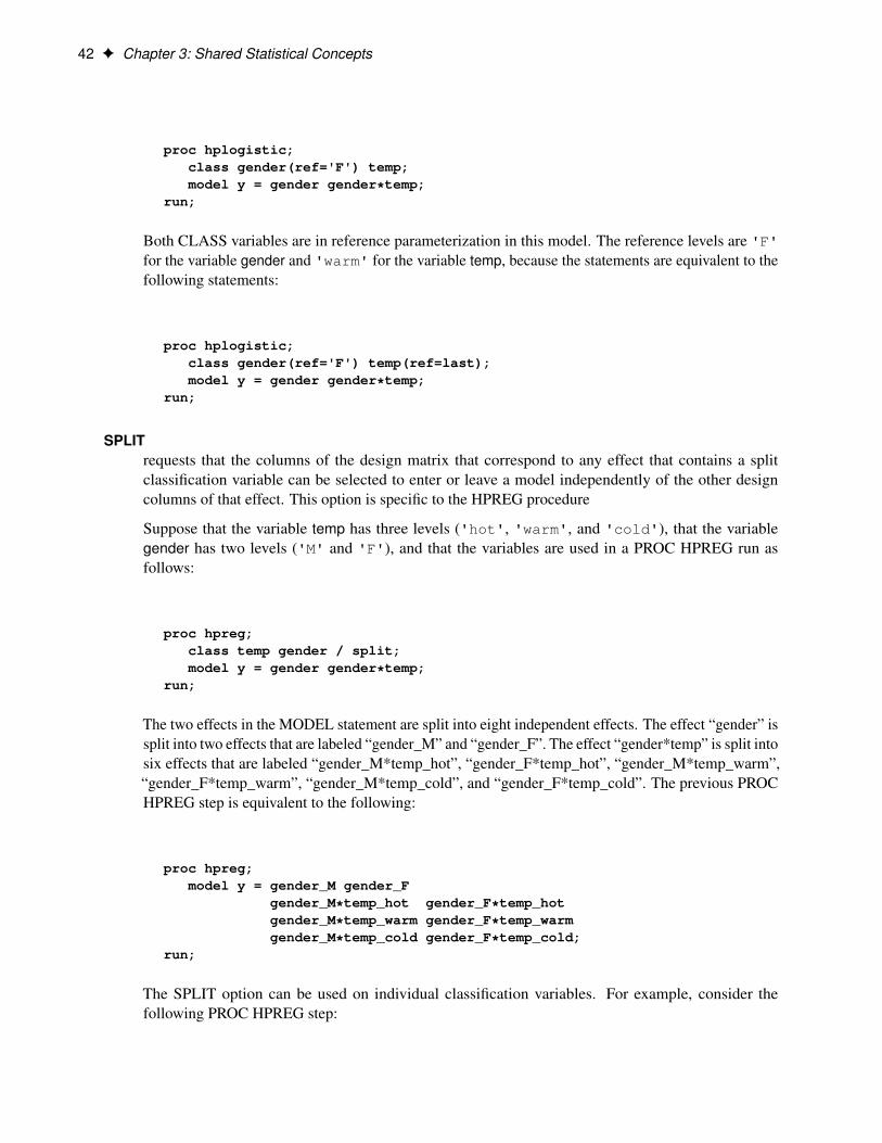
42 F Chapter 3: Shared Statistical Concepts
proc hplogistic;class gender(ref='F') temp;model y = gender gender*temp;
run;
Both CLASS variables are in reference parameterization in this model. The reference levels are 'F'for the variable gender and 'warm' for the variable temp, because the statements are equivalent to thefollowing statements:
proc hplogistic;class gender(ref='F') temp(ref=last);model y = gender gender*temp;
run;
SPLITrequests that the columns of the design matrix that correspond to any effect that contains a splitclassification variable can be selected to enter or leave a model independently of the other designcolumns of that effect. This option is specific to the HPREG procedure
Suppose that the variable temp has three levels ('hot', 'warm', and 'cold'), that the variablegender has two levels ('M' and 'F'), and that the variables are used in a PROC HPREG run asfollows:
proc hpreg;class temp gender / split;model y = gender gender*temp;
run;
The two effects in the MODEL statement are split into eight independent effects. The effect “gender” issplit into two effects that are labeled “gender_M” and “gender_F”. The effect “gender*temp” is split intosix effects that are labeled “gender_M*temp_hot”, “gender_F*temp_hot”, “gender_M*temp_warm”,“gender_F*temp_warm”, “gender_M*temp_cold”, and “gender_F*temp_cold”. The previous PROCHPREG step is equivalent to the following:
proc hpreg;model y = gender_M gender_F
gender_M*temp_hot gender_F*temp_hotgender_M*temp_warm gender_F*temp_warmgender_M*temp_cold gender_F*temp_cold;
run;
The SPLIT option can be used on individual classification variables. For example, consider thefollowing PROC HPREG step:

CLASS Statement F 43
proc hpreg;class temp(split) gender;model y = gender gender*temp;
run;
In this case, the effect “gender” is not split and the effect “gender*temp” is split into three effects,which are labeled “gender*temp_hot”, “gender*temp_warm”, and “gender*temp_cold”. Furthermore,each of these three split effects now has two parameters that correspond to the two levels of “gender.”The PROC HPREG step is equivalent to the following:
proc hpreg;class gender;model y = gender gender*temp_hot gender*temp_warm gender*temp_cold;
run;
You can specify the following global-options:
MISSINGtreats missing values (“.”, “.A”, . . . , “.Z” for numeric variables and blanks for character variables) asvalid values for the CLASS variable.
If you do not specify the MISSING option, observations that have missing values for CLASS variablesare removed from the analysis, even if the CLASS variables are not used in the model formulation.
PARAM=keywordspecifies the parameterization method for the classification variable or variables. You can specify thefollowing keywords:
GLM specifies a less-than-full-rank reference cell coding. This parameterization is used in, forexample, the GLM, MIXED, and GLIMMIX procedures in SAS/STAT.
REFERENCE specifies a reference cell encoding. You can choose the reference value by specifyingan option for a specific variable or set of variables in the CLASS statement, or designatethe first or last ordered value by specifying a global-option. The default is REF=LAST.
For example, suppose that the variable temp has three levels ('hot', 'warm', and'cold'), that the variable gender has two levels ('M' and 'F'), and that the variables areused in a CLASS statement as follows:
class gender(ref='F') temp / param=ref;
Then 'F' is used as the reference level for gender and 'warm' is used as the referencelevel for temp.
The GLM parameterization is the default. For more information about how parameterization ofclassification variables affects the construction and interpretation of model effects, see the section“Specification and Parameterization of Model Effects” on page 52.

44 F Chapter 3: Shared Statistical Concepts
TRUNCATE< =n >specifies the truncation width of formatted values of CLASS variables when the optional n is specified.
If n is not specified, the TRUNCATE option requests that classification levels be determined by usingno more than the first 16 characters of the formatted values of CLASS variables.
FREQ StatementFREQ variable ;
The variable in the FREQ statement identifies a numeric variable in the data set that contains the frequency ofoccurrence for each observation. High-performance statistical procedures that support the FREQ statementtreat each observation as if it appeared f times, where f is the value of the FREQ variable for the observation.If the frequency value is not an integer, it is truncated to an integer. If the frequency value is less than 1or missing, the observation is not used in the analysis. When the FREQ statement is not specified, eachobservation is assigned a frequency of 1.
ID StatementID variables ;
The ID statement lists one or more variables from the input data set that are transferred to output data setsthat are created by high-performance statistical procedures, provided that the output data set contains one(or more) records per input observation. For example, when an OUTPUT statement is used to produceobservationwise scores or prediction statistics, ID variables are added to the output data set.
By default, high-performance statistical procedures do not include all variables from the input data setin output data sets. In the following statements, a logistic regression model is fit and then scored. Theinput and output data are stored in the Greenplum database. The output data set contains three columns (p,account, trans_date) where p is computed during the scoring process and the account and transaction dateare transferred from the input data set. (High-performance statistical procedures also transfer any distributionkeys from the input to the output data.)
libname GPLib greenplm server=gpdca user=XXX password=YYYdatabase=ZZZ;
proc hplogistic data=gplib.myData;class a b;model y = a b x1-x20;output out=gplib.scores pred=p;id account trans_date;
run;
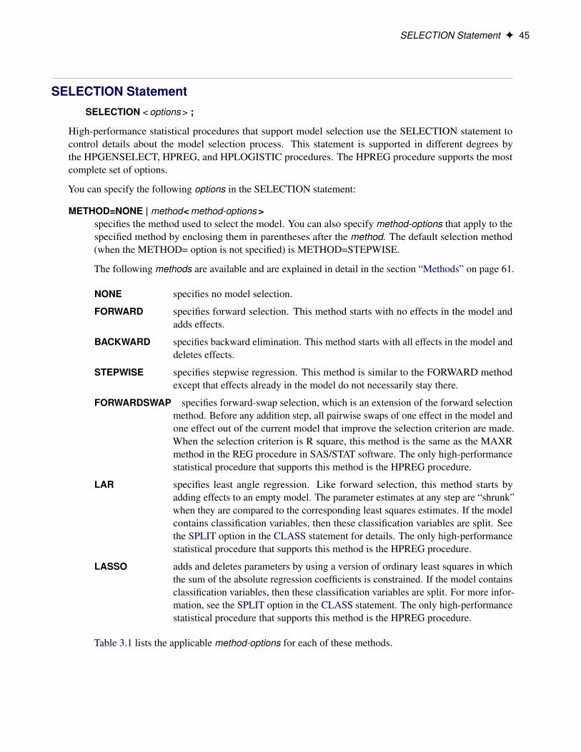
SELECTION Statement F 45
SELECTION StatementSELECTION < options > ;
High-performance statistical procedures that support model selection use the SELECTION statement tocontrol details about the model selection process. This statement is supported in different degrees bythe HPGENSELECT, HPREG, and HPLOGISTIC procedures. The HPREG procedure supports the mostcomplete set of options.
You can specify the following options in the SELECTION statement:
METHOD=NONE | method< method-options >specifies the method used to select the model. You can also specify method-options that apply to thespecified method by enclosing them in parentheses after the method. The default selection method(when the METHOD= option is not specified) is METHOD=STEPWISE.
The following methods are available and are explained in detail in the section “Methods” on page 61.
NONE specifies no model selection.
FORWARD specifies forward selection. This method starts with no effects in the model andadds effects.
BACKWARD specifies backward elimination. This method starts with all effects in the model anddeletes effects.
STEPWISE specifies stepwise regression. This method is similar to the FORWARD methodexcept that effects already in the model do not necessarily stay there.
FORWARDSWAP specifies forward-swap selection, which is an extension of the forward selectionmethod. Before any addition step, all pairwise swaps of one effect in the model andone effect out of the current model that improve the selection criterion are made.When the selection criterion is R square, this method is the same as the MAXRmethod in the REG procedure in SAS/STAT software. The only high-performancestatistical procedure that supports this method is the HPREG procedure.
LAR specifies least angle regression. Like forward selection, this method starts byadding effects to an empty model. The parameter estimates at any step are “shrunk”when they are compared to the corresponding least squares estimates. If the modelcontains classification variables, then these classification variables are split. Seethe SPLIT option in the CLASS statement for details. The only high-performancestatistical procedure that supports this method is the HPREG procedure.
LASSO adds and deletes parameters by using a version of ordinary least squares in whichthe sum of the absolute regression coefficients is constrained. If the model containsclassification variables, then these classification variables are split. For more infor-mation, see the SPLIT option in the CLASS statement. The only high-performancestatistical procedure that supports this method is the HPREG procedure.
Table 3.1 lists the applicable method-options for each of these methods.
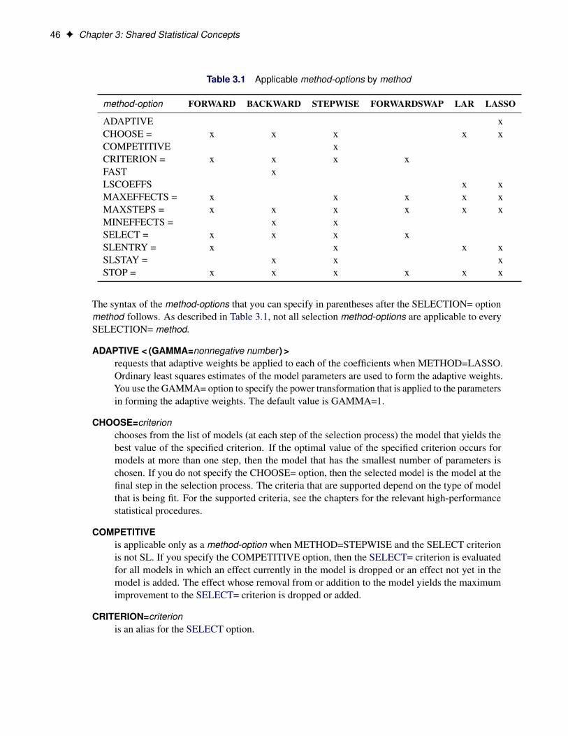
46 F Chapter 3: Shared Statistical Concepts
Table 3.1 Applicable method-options by method
method-option FORWARD BACKWARD STEPWISE FORWARDSWAP LAR LASSO
ADAPTIVE xCHOOSE = x x x x xCOMPETITIVE xCRITERION = x x x xFAST xLSCOEFFS x xMAXEFFECTS = x x x x xMAXSTEPS = x x x x x xMINEFFECTS = x xSELECT = x x x xSLENTRY = x x x xSLSTAY = x x xSTOP = x x x x x x
The syntax of the method-options that you can specify in parentheses after the SELECTION= optionmethod follows. As described in Table 3.1, not all selection method-options are applicable to everySELECTION= method.
ADAPTIVE < (GAMMA=nonnegative number ) >requests that adaptive weights be applied to each of the coefficients when METHOD=LASSO.Ordinary least squares estimates of the model parameters are used to form the adaptive weights.You use the GAMMA= option to specify the power transformation that is applied to the parametersin forming the adaptive weights. The default value is GAMMA=1.
CHOOSE=criterionchooses from the list of models (at each step of the selection process) the model that yields thebest value of the specified criterion. If the optimal value of the specified criterion occurs formodels at more than one step, then the model that has the smallest number of parameters ischosen. If you do not specify the CHOOSE= option, then the selected model is the model at thefinal step in the selection process. The criteria that are supported depend on the type of modelthat is being fit. For the supported criteria, see the chapters for the relevant high-performancestatistical procedures.
COMPETITIVEis applicable only as a method-option when METHOD=STEPWISE and the SELECT criterionis not SL. If you specify the COMPETITIVE option, then the SELECT= criterion is evaluatedfor all models in which an effect currently in the model is dropped or an effect not yet in themodel is added. The effect whose removal from or addition to the model yields the maximumimprovement to the SELECT= criterion is dropped or added.
CRITERION=criterionis an alias for the SELECT option.
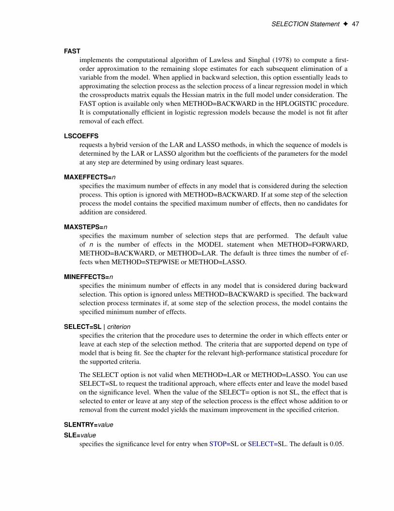
SELECTION Statement F 47
FASTimplements the computational algorithm of Lawless and Singhal (1978) to compute a first-order approximation to the remaining slope estimates for each subsequent elimination of avariable from the model. When applied in backward selection, this option essentially leads toapproximating the selection process as the selection process of a linear regression model in whichthe crossproducts matrix equals the Hessian matrix in the full model under consideration. TheFAST option is available only when METHOD=BACKWARD in the HPLOGISTIC procedure.It is computationally efficient in logistic regression models because the model is not fit afterremoval of each effect.
LSCOEFFSrequests a hybrid version of the LAR and LASSO methods, in which the sequence of models isdetermined by the LAR or LASSO algorithm but the coefficients of the parameters for the modelat any step are determined by using ordinary least squares.
MAXEFFECTS=nspecifies the maximum number of effects in any model that is considered during the selectionprocess. This option is ignored with METHOD=BACKWARD. If at some step of the selectionprocess the model contains the specified maximum number of effects, then no candidates foraddition are considered.
MAXSTEPS=nspecifies the maximum number of selection steps that are performed. The default valueof n is the number of effects in the MODEL statement when METHOD=FORWARD,METHOD=BACKWARD, or METHOD=LAR. The default is three times the number of ef-fects when METHOD=STEPWISE or METHOD=LASSO.
MINEFFECTS=nspecifies the minimum number of effects in any model that is considered during backwardselection. This option is ignored unless METHOD=BACKWARD is specified. The backwardselection process terminates if, at some step of the selection process, the model contains thespecified minimum number of effects.
SELECT=SL | criterionspecifies the criterion that the procedure uses to determine the order in which effects enter orleave at each step of the selection method. The criteria that are supported depend on type ofmodel that is being fit. See the chapter for the relevant high-performance statistical procedure forthe supported criteria.
The SELECT option is not valid when METHOD=LAR or METHOD=LASSO. You can useSELECT=SL to request the traditional approach, where effects enter and leave the model basedon the significance level. When the value of the SELECT= option is not SL, the effect that isselected to enter or leave at any step of the selection process is the effect whose addition to orremoval from the current model yields the maximum improvement in the specified criterion.
SLENTRY=value
SLE=valuespecifies the significance level for entry when STOP=SL or SELECT=SL. The default is 0.05.

48 F Chapter 3: Shared Statistical Concepts
SLSTAY=value
SLS=valuespecifies the significance level for staying in the model when STOP=SL or SELECT=SL. Thedefault is 0.05.
STOP=SL | NONE | criterionspecifies a criterion that is used to stop the selection process. The criteria that are supporteddepend on the type of model that is being fit. For information about the supported criteria, seethe chapter about the relevant high-performance statistical procedure.
If you do not specify the STOP= option but do specify the SELECT= option, then the criterionspecified in the SELECT= option is also used as the STOP= criterion.
If you specify STOP=NONE, then the selection process stops if no suitable add or drop candidatescan be found or if a size-based limit is reached. For example, if you specify STOP=NONEMAXEFFECTS=5, then the selection process stops at the first step that produces a model withfive effects.
When STOP=SL, selection stops at the step where the significance level of the candidate forentry is greater than the SLENTRY= value for addition steps when METHOD=FORWARD orMETHOD=STEPWISE and where the significance level of the candidate for removal is greaterthan the SLSTAY= value when METHOD=BACKWARD or METHOD=STEPWISE.
If you specify a criterion other than SL for the STOP= option, then the selection process stopsif the selection process produces a local extremum of this criterion or if a size-based limit isreached. For example, if you specify STOP=AIC MAXSTEPS=5, then the selection processstops before step 5 if the sequence of models has a local minimum of the AIC criterion beforestep 5. The determination of whether a local minimum is reached is made on the basis of a stophorizon. The default stop horizon is 3, but you can change it by using the STOPHORIZON=option. If the stop horizon is n and the STOP= criterion at any step is better than the stop criterionat the next n steps, then the selection process terminates.
DETAILS=NONE | SUMMARY | ALL
DETAILS=STEPS< CANDIDATES(ALL | n) >specifies the level of detail to be produced about the selection process. The default is DE-TAILS=SUMMARY.
The DETAILS=ALL and DETAILS=STEPS options produce the following output:
• tables that provide information about the model that is selected at each step of the selectionprocess.
• entry and removal statistics for inclusion or exclusion candidates at each step. By default, onlythe top 10 candidates at each step are shown. If you specify STEPS(CANDIDATES(n)), then thebest n candidates are shown. If you specify STEPS(CANDIDATES(ALL)), then all candidatesare shown.
• a selection summary table that shows by step the effect that is added to or removed from themodel in addition to the values of the SELECT, STOP, and CHOOSE criteria for the resultingmodel.
• a stop reason table that describes why the selection process stopped.
SELECTION Statement F 49
• a selection reason table that describes why the selected model was chosen.
• a selected effects table that lists the effects that are in the selected model.
The DETAILS=SUMMARY option produces only the selection summary, stop reason, selection reason,and selected effects tables.
HIERARCHY=NONE | SINGLE | SINGLECLASSspecifies whether and how the model hierarchy requirement is applied. This option also controlswhether a single effect or multiple effects are allowed to enter or leave the model in one step. Youcan specify that only classification effects, or both classification and continuous effects, be subject tothe hierarchy requirement. The HIERARCHY= option is ignored unless you also specify one of thefollowing options: METHOD=FORWARD, METHOD=BACKWARD, or METHOD=STEPWISE.
Model hierarchy refers to the requirement that, for any term to be in the model, all model effects thatare contained in the term must be present in the model. For example, in order for the interaction A*Bto enter the model, the main effects A and B must be in the model. Likewise, neither effect A nor effectB can leave the model while the interaction A*B is in the model.
You can specify the following values:
NONE specifies that model hierarchy not be maintained. Any single effect can enter orleave the model at any given step of the selection process.
SINGLE specifies that only one effect enter or leave the model at one time, subject to themodel hierarchy requirement. For example, suppose that the model contains themain effects A and B and the interaction A*B. In the first step of the selectionprocess, either A or B can enter the model. In the second step, the other main effectcan enter the model. The interaction effect can enter the model only when bothmain effects have already entered. Also, before A or B can be removed from themodel, the A*B interaction must first be removed. All effects (CLASS and interval)are subject to the hierarchy requirement.
SINGLECLASS is the same as HIERARCHY=SINGLE except that only CLASS effects are subjectto the hierarchy requirement.
The default value is HIERARCHY=NONE.
SELECTION=NONE | BACKWARD | FORWARD | FORWARDSWAP | STEPWISE | LAR | LASSOis an alias for the METHOD= option.
STOPHORIZON=nspecifies the number of consecutive steps at which the STOP= criterion must worsen in order for alocal extremum to be detected. The default value is STOPHORIZON=3. The stop horizon value isignored if you also specify STOP=NONE or STOP=SL. For example, suppose that STOP=AIC andthe sequence of AIC values at steps 1 to 6 of a selection are 10, 7, 4, 6, 5, 2. If STOPHORIZON=2,then the AIC criterion is deemed to have a local minimum at step 3 because the AIC value at the nexttwo steps are greater than the value 4 that occurs at step 3. However, if STOPHORIZON=3, then thevalue at step 3 is not deemed to be a local minimum because the AIC value at step 6 is lower than theAIC value at step 3.
50 F Chapter 3: Shared Statistical Concepts
VAR StatementVAR variable-list ;
Some high-performance statistical procedures (in particular procedures that do not support a MODELstatement) use a VAR statement to identify numerical variables for the analysis.
WEIGHT StatementWEIGHT variable ;
The variable in the WEIGHT statement is used as a weight to perform a weighted analysis of the data.Observations with nonpositive or missing weights are not included in the analysis. If a WEIGHT statement isnot included, all observations that are used in the analysis are assigned a weight of 1.
Levelization of Classification VariablesA classification variable enters the statistical analysis or model not through its values but through its levels.The process of associating values of a variable with levels is termed levelization.
During the process of levelization, observations that share the same value are assigned to the same level.The manner in which values are grouped can be affected by the inclusion of formats. The sort order of thelevels can be determined by specifying the ORDER= option in the procedure statement. In high-performancestatistical procedures, you can also control the sorting order separately for each variable in the CLASSstatement.
Consider the data on nine observations in Table 3.2. The variable A is integer-valued, and the variable X isa continuous variable that has a missing value for the fourth observation. The fourth and fifth columns ofTable 3.2 apply two different formats to the variable X.
Table 3.2 Example Data for Levelization
Obs A x FORMATx 3.0
FORMATx 3.1
1 2 1.09 1 1.12 2 1.13 1 1.13 2 1.27 1 1.34 3 . . .5 3 2.26 2 2.36 3 2.48 2 2.57 4 3.34 3 3.38 4 3.34 3 3.39 4 3.14 3 3.1

Levelization of Classification Variables F 51
By default, levelization of the variables groups the observations by the formatted value of the variable, exceptfor numerical variables for which no explicit format is provided. Numerical variables for which no explicitformat is provided are sorted by their internal value. The levelization of the four columns in Table 3.2 leadsto the level assignment in Table 3.3.
Table 3.3 Values and Levels
A X FORMAT x 3.0 FORMAT x 3.1Obs Value Level Value Level Value Level Value Level
1 2 1 1.09 1 1 1 1.1 12 2 1 1.13 2 1 1 1.1 13 2 1 1.27 3 1 1 1.3 24 3 2 . . . . . .5 3 2 2.26 4 2 2 2.3 36 3 2 2.48 5 2 2 2.5 47 4 3 3.34 7 3 3 3.3 68 4 3 3.34 7 3 3 3.3 69 4 3 3.14 6 3 3 3.1 5
The sort order for the levels of CLASS variables can be specified in the ORDER= option in the CLASSstatement.
When ORDER=FORMATTED (which is the default) is in effect for numeric variables for which you havesupplied no explicit format, the levels are ordered by their internal values. To order numeric class levels thathave no explicit format by their BEST12. formatted values, you can specify the BEST12. format explicitlyfor the CLASS variables.
Table 3.4 shows how values of the ORDER= option are interpreted.
Table 3.4 Interpretation of Values of ORDER= Option
Value of ORDER= Levels Sorted By
DATA Order of appearance in the input data set
FORMATTED External formatted value, except for numeric variablesthat have no explicit format, which are sorted by theirunformatted (internal) value
FREQ Descending frequency count (levels that have the mostobservations come first in the order)
INTERNAL Unformatted value
FREQDATA Order of descending frequency count, and within countsby order of appearance in the input data set when countsare tied
FREQFORMATTED Order of descending frequency count, and within countsby formatted value when counts are tied
FREQINTERNAL Order of descending frequency count, and within countsby unformatted (internal) value when counts are tied
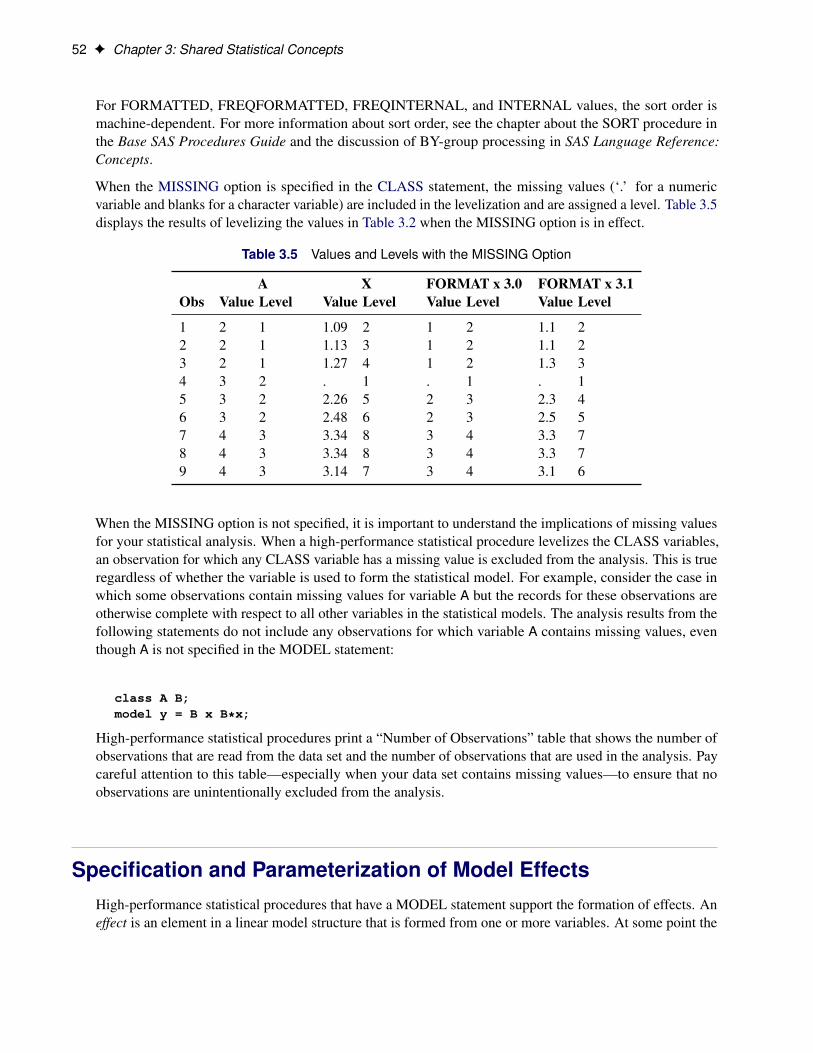
52 F Chapter 3: Shared Statistical Concepts
For FORMATTED, FREQFORMATTED, FREQINTERNAL, and INTERNAL values, the sort order ismachine-dependent. For more information about sort order, see the chapter about the SORT procedure inthe Base SAS Procedures Guide and the discussion of BY-group processing in SAS Language Reference:Concepts.
When the MISSING option is specified in the CLASS statement, the missing values (‘.’ for a numericvariable and blanks for a character variable) are included in the levelization and are assigned a level. Table 3.5displays the results of levelizing the values in Table 3.2 when the MISSING option is in effect.
Table 3.5 Values and Levels with the MISSING Option
A X FORMAT x 3.0 FORMAT x 3.1Obs Value Level Value Level Value Level Value Level
1 2 1 1.09 2 1 2 1.1 22 2 1 1.13 3 1 2 1.1 23 2 1 1.27 4 1 2 1.3 34 3 2 . 1 . 1 . 15 3 2 2.26 5 2 3 2.3 46 3 2 2.48 6 2 3 2.5 57 4 3 3.34 8 3 4 3.3 78 4 3 3.34 8 3 4 3.3 79 4 3 3.14 7 3 4 3.1 6
When the MISSING option is not specified, it is important to understand the implications of missing valuesfor your statistical analysis. When a high-performance statistical procedure levelizes the CLASS variables,an observation for which any CLASS variable has a missing value is excluded from the analysis. This is trueregardless of whether the variable is used to form the statistical model. For example, consider the case inwhich some observations contain missing values for variable A but the records for these observations areotherwise complete with respect to all other variables in the statistical models. The analysis results from thefollowing statements do not include any observations for which variable A contains missing values, eventhough A is not specified in the MODEL statement:
class A B;model y = B x B*x;
High-performance statistical procedures print a “Number of Observations” table that shows the number ofobservations that are read from the data set and the number of observations that are used in the analysis. Paycareful attention to this table—especially when your data set contains missing values—to ensure that noobservations are unintentionally excluded from the analysis.
Specification and Parameterization of Model EffectsHigh-performance statistical procedures that have a MODEL statement support the formation of effects. Aneffect is an element in a linear model structure that is formed from one or more variables. At some point the
Effect Operators F 53
statistical representations of these models involve linear structures such as
Xˇ
or
Xˇ C Z
The model matrices X and Z are formed according to effect construction rules.
Procedures that also have a CLASS statement support the rich set of effects that is discussed in this section.In order to correctly interpret the results from a statistical analysis, you need to understand how construction(parameterization) rules apply to regression-type models, whether these are linear models in the HPREGprocedure or generalized linear models in the HPLOGISTIC procedure.
Effects are specified by a special notation that uses variable names and operators. There are two typesof variables: classification (or CLASS) variables and continuous variables. Classification variables canbe either numeric or character and are specified in a CLASS statement. For more information, see thesection “Levelization of Classification Variables” on page 50. An independent variable that is not declared inthe CLASS statement is assumed to be continuous. For example, the heights and weights of subjects arecontinuous variables.
Two primary operators (crossing and nesting) are used for combining the variables, and several additionaloperators are used to simplify effect specification. Operators are discussed in the section “Effect Operators”on page 53.
High-performance statistical procedures that have a CLASS statement support a general linear model (GLM)parameterization and a reference parameterization for the classification variables. The GLM parameterizationis the default for all high-performance statistical procedures. For more information, see the sections “GLMParameterization of Classification Variables and Effects” on page 55 and “Reference Parameterization” onpage 60.
Effect OperatorsTable 3.6 summarizes the operators that are available for selecting and constructing effects. These operatorsare discussed in the following sections.
Table 3.6 Available Effect Operators
Operator Example Description
Interaction A*B Crosses the levels of the effectsNesting A(B) Nests A levels within B levelsBar operator A | B | C Specifies all interactionsAt sign operator A | B | C@2 Reduces interactions in bar effectsDash operator A1-A10 Specifies sequentially numbered variablesColon operator A: Specifies variables with common prefixDouble dash operator A- -C Specifies sequential variables in data set order
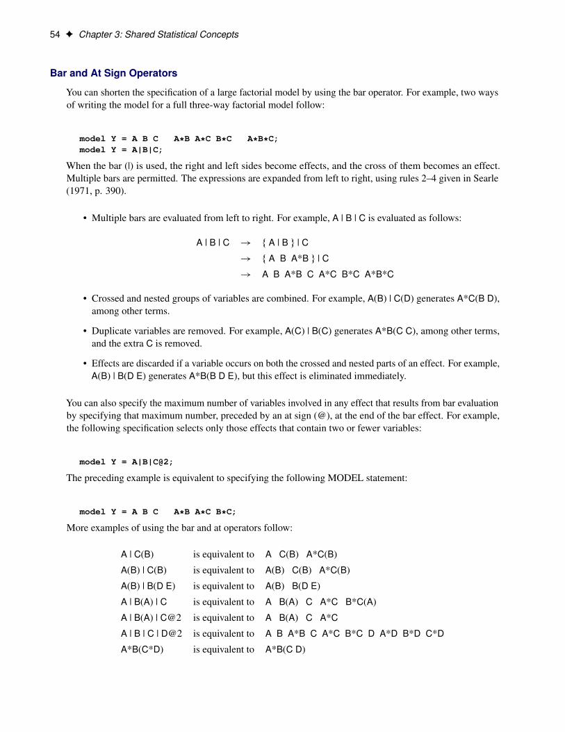
54 F Chapter 3: Shared Statistical Concepts
Bar and At Sign Operators
You can shorten the specification of a large factorial model by using the bar operator. For example, two waysof writing the model for a full three-way factorial model follow:
model Y = A B C A*B A*C B*C A*B*C;model Y = A|B|C;
When the bar (|) is used, the right and left sides become effects, and the cross of them becomes an effect.Multiple bars are permitted. The expressions are expanded from left to right, using rules 2–4 given in Searle(1971, p. 390).
• Multiple bars are evaluated from left to right. For example, A | B | C is evaluated as follows:
A | B | C ! f A | B g | C
! f A B A*B g | C
! A B A*B C A*C B*C A*B*C
• Crossed and nested groups of variables are combined. For example, A(B) | C(D) generates A*C(B D),among other terms.
• Duplicate variables are removed. For example, A(C) | B(C) generates A*B(C C), among other terms,and the extra C is removed.
• Effects are discarded if a variable occurs on both the crossed and nested parts of an effect. For example,A(B) | B(D E) generates A*B(B D E), but this effect is eliminated immediately.
You can also specify the maximum number of variables involved in any effect that results from bar evaluationby specifying that maximum number, preceded by an at sign (@), at the end of the bar effect. For example,the following specification selects only those effects that contain two or fewer variables:
model Y = A|B|C@2;
The preceding example is equivalent to specifying the following MODEL statement:
model Y = A B C A*B A*C B*C;
More examples of using the bar and at operators follow:
A | C(B) is equivalent to A C(B) A*C(B)
A(B) | C(B) is equivalent to A(B) C(B) A*C(B)
A(B) | B(D E) is equivalent to A(B) B(D E)
A | B(A) | C is equivalent to A B(A) C A*C B*C(A)
A | B(A) | C@2 is equivalent to A B(A) C A*C
A | B | C | D@2 is equivalent to A B A*B C A*C B*C D A*D B*D C*D
A*B(C*D) is equivalent to A*B(C D)
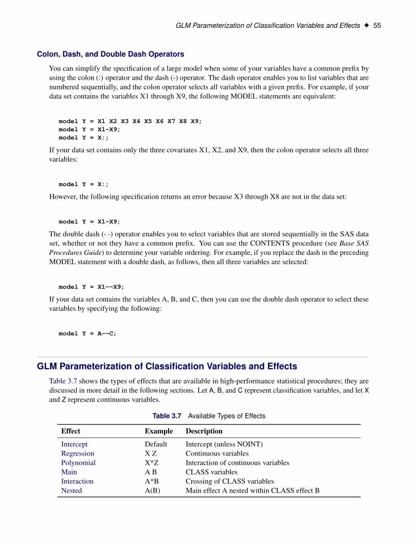
GLM Parameterization of Classification Variables and Effects F 55
Colon, Dash, and Double Dash Operators
You can simplify the specification of a large model when some of your variables have a common prefix byusing the colon (:) operator and the dash (-) operator. The dash operator enables you to list variables that arenumbered sequentially, and the colon operator selects all variables with a given prefix. For example, if yourdata set contains the variables X1 through X9, the following MODEL statements are equivalent:
model Y = X1 X2 X3 X4 X5 X6 X7 X8 X9;model Y = X1-X9;model Y = X:;
If your data set contains only the three covariates X1, X2, and X9, then the colon operator selects all threevariables:
model Y = X:;
However, the following specification returns an error because X3 through X8 are not in the data set:
model Y = X1-X9;
The double dash (- -) operator enables you to select variables that are stored sequentially in the SAS dataset, whether or not they have a common prefix. You can use the CONTENTS procedure (see Base SASProcedures Guide) to determine your variable ordering. For example, if you replace the dash in the precedingMODEL statement with a double dash, as follows, then all three variables are selected:
model Y = X1--X9;
If your data set contains the variables A, B, and C, then you can use the double dash operator to select thesevariables by specifying the following:
model Y = A--C;
GLM Parameterization of Classification Variables and EffectsTable 3.7 shows the types of effects that are available in high-performance statistical procedures; they arediscussed in more detail in the following sections. Let A, B, and C represent classification variables, and let Xand Z represent continuous variables.
Table 3.7 Available Types of Effects
Effect Example Description
Intercept Default Intercept (unless NOINT)Regression X Z Continuous variablesPolynomial X*Z Interaction of continuous variablesMain A B CLASS variablesInteraction A*B Crossing of CLASS variablesNested A(B) Main effect A nested within CLASS effect B
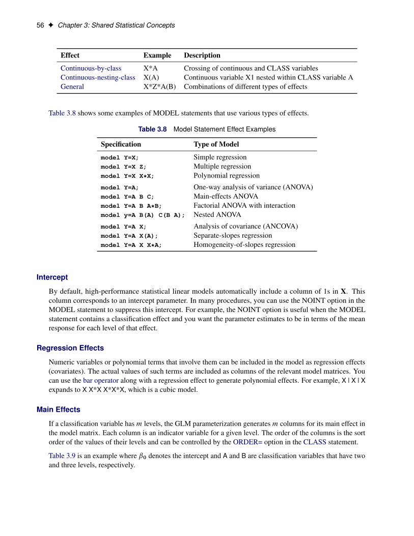
56 F Chapter 3: Shared Statistical Concepts
Effect Example Description
Continuous-by-class X*A Crossing of continuous and CLASS variablesContinuous-nesting-class X(A) Continuous variable X1 nested within CLASS variable AGeneral X*Z*A(B) Combinations of different types of effects
Table 3.8 shows some examples of MODEL statements that use various types of effects.
Table 3.8 Model Statement Effect Examples
Specification Type of Model
model Y=X; Simple regressionmodel Y=X Z; Multiple regressionmodel Y=X X*X; Polynomial regression
model Y=A; One-way analysis of variance (ANOVA)model Y=A B C; Main-effects ANOVAmodel Y=A B A*B; Factorial ANOVA with interactionmodel y=A B(A) C(B A); Nested ANOVA
model Y=A X; Analysis of covariance (ANCOVA)model Y=A X(A); Separate-slopes regressionmodel Y=A X X*A; Homogeneity-of-slopes regression
Intercept
By default, high-performance statistical linear models automatically include a column of 1s in X. Thiscolumn corresponds to an intercept parameter. In many procedures, you can use the NOINT option in theMODEL statement to suppress this intercept. For example, the NOINT option is useful when the MODELstatement contains a classification effect and you want the parameter estimates to be in terms of the meanresponse for each level of that effect.
Regression Effects
Numeric variables or polynomial terms that involve them can be included in the model as regression effects(covariates). The actual values of such terms are included as columns of the relevant model matrices. Youcan use the bar operator along with a regression effect to generate polynomial effects. For example, X | X | Xexpands to X X*X X*X*X, which is a cubic model.
Main Effects
If a classification variable has m levels, the GLM parameterization generates m columns for its main effect inthe model matrix. Each column is an indicator variable for a given level. The order of the columns is the sortorder of the values of their levels and can be controlled by the ORDER= option in the CLASS statement.
Table 3.9 is an example where ˇ0 denotes the intercept and A and B are classification variables that have twoand three levels, respectively.
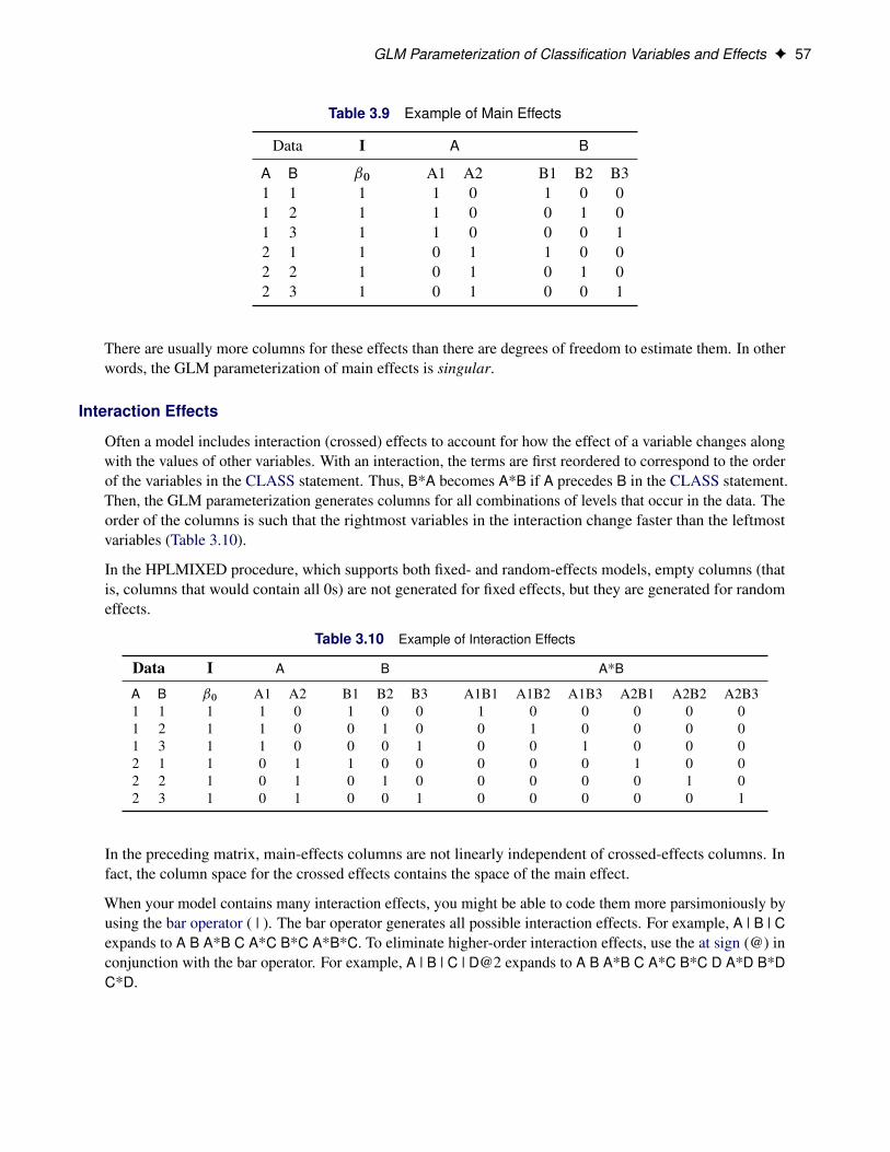
GLM Parameterization of Classification Variables and Effects F 57
Table 3.9 Example of Main Effects
Data I A B
A B ˇ0 A1 A2 B1 B2 B31 1 1 1 0 1 0 01 2 1 1 0 0 1 01 3 1 1 0 0 0 12 1 1 0 1 1 0 02 2 1 0 1 0 1 02 3 1 0 1 0 0 1
There are usually more columns for these effects than there are degrees of freedom to estimate them. In otherwords, the GLM parameterization of main effects is singular.
Interaction Effects
Often a model includes interaction (crossed) effects to account for how the effect of a variable changes alongwith the values of other variables. With an interaction, the terms are first reordered to correspond to the orderof the variables in the CLASS statement. Thus, B*A becomes A*B if A precedes B in the CLASS statement.Then, the GLM parameterization generates columns for all combinations of levels that occur in the data. Theorder of the columns is such that the rightmost variables in the interaction change faster than the leftmostvariables (Table 3.10).
In the HPLMIXED procedure, which supports both fixed- and random-effects models, empty columns (thatis, columns that would contain all 0s) are not generated for fixed effects, but they are generated for randomeffects.
Table 3.10 Example of Interaction Effects
Data I A B A*B
A B ˇ0 A1 A2 B1 B2 B3 A1B1 A1B2 A1B3 A2B1 A2B2 A2B31 1 1 1 0 1 0 0 1 0 0 0 0 01 2 1 1 0 0 1 0 0 1 0 0 0 01 3 1 1 0 0 0 1 0 0 1 0 0 02 1 1 0 1 1 0 0 0 0 0 1 0 02 2 1 0 1 0 1 0 0 0 0 0 1 02 3 1 0 1 0 0 1 0 0 0 0 0 1
In the preceding matrix, main-effects columns are not linearly independent of crossed-effects columns. Infact, the column space for the crossed effects contains the space of the main effect.
When your model contains many interaction effects, you might be able to code them more parsimoniously byusing the bar operator ( | ). The bar operator generates all possible interaction effects. For example, A | B | Cexpands to A B A*B C A*C B*C A*B*C. To eliminate higher-order interaction effects, use the at sign (@) inconjunction with the bar operator. For example, A | B | C | D@2 expands to A B A*B C A*C B*C D A*D B*DC*D.
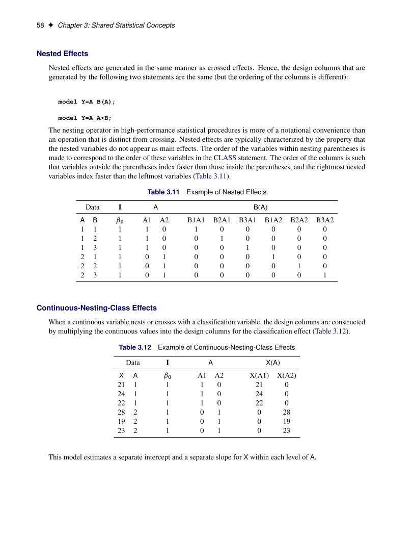
58 F Chapter 3: Shared Statistical Concepts
Nested Effects
Nested effects are generated in the same manner as crossed effects. Hence, the design columns that aregenerated by the following two statements are the same (but the ordering of the columns is different):
model Y=A B(A);
model Y=A A*B;
The nesting operator in high-performance statistical procedures is more of a notational convenience thanan operation that is distinct from crossing. Nested effects are typically characterized by the property thatthe nested variables do not appear as main effects. The order of the variables within nesting parentheses ismade to correspond to the order of these variables in the CLASS statement. The order of the columns is suchthat variables outside the parentheses index faster than those inside the parentheses, and the rightmost nestedvariables index faster than the leftmost variables (Table 3.11).
Table 3.11 Example of Nested Effects
Data I A B(A)
A B ˇ0 A1 A2 B1A1 B2A1 B3A1 B1A2 B2A2 B3A21 1 1 1 0 1 0 0 0 0 01 2 1 1 0 0 1 0 0 0 01 3 1 1 0 0 0 1 0 0 02 1 1 0 1 0 0 0 1 0 02 2 1 0 1 0 0 0 0 1 02 3 1 0 1 0 0 0 0 0 1
Continuous-Nesting-Class Effects
When a continuous variable nests or crosses with a classification variable, the design columns are constructedby multiplying the continuous values into the design columns for the classification effect (Table 3.12).
Table 3.12 Example of Continuous-Nesting-Class Effects
Data I A X(A)
X A ˇ0 A1 A2 X(A1) X(A2)21 1 1 1 0 21 024 1 1 1 0 24 022 1 1 1 0 22 028 2 1 0 1 0 2819 2 1 0 1 0 1923 2 1 0 1 0 23
This model estimates a separate intercept and a separate slope for X within each level of A.
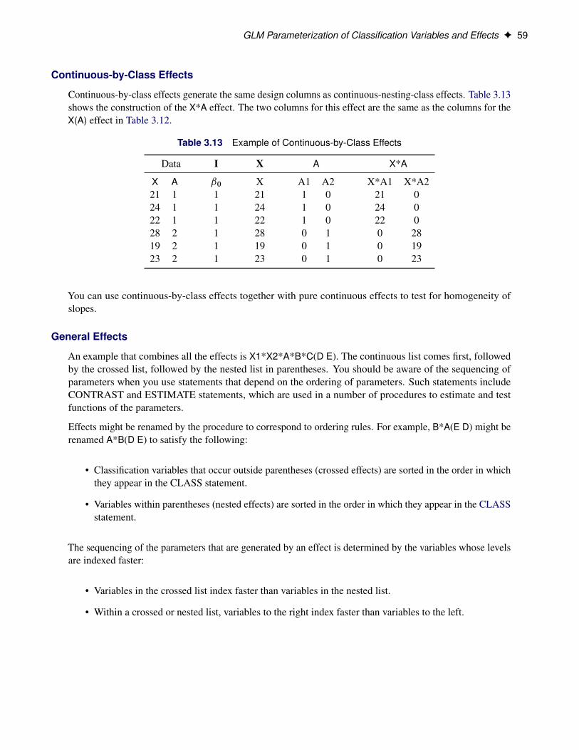
GLM Parameterization of Classification Variables and Effects F 59
Continuous-by-Class Effects
Continuous-by-class effects generate the same design columns as continuous-nesting-class effects. Table 3.13shows the construction of the X*A effect. The two columns for this effect are the same as the columns for theX(A) effect in Table 3.12.
Table 3.13 Example of Continuous-by-Class Effects
Data I X A X*A
X A ˇ0 X A1 A2 X*A1 X*A221 1 1 21 1 0 21 024 1 1 24 1 0 24 022 1 1 22 1 0 22 028 2 1 28 0 1 0 2819 2 1 19 0 1 0 1923 2 1 23 0 1 0 23
You can use continuous-by-class effects together with pure continuous effects to test for homogeneity ofslopes.
General Effects
An example that combines all the effects is X1*X2*A*B*C(D E). The continuous list comes first, followedby the crossed list, followed by the nested list in parentheses. You should be aware of the sequencing ofparameters when you use statements that depend on the ordering of parameters. Such statements includeCONTRAST and ESTIMATE statements, which are used in a number of procedures to estimate and testfunctions of the parameters.
Effects might be renamed by the procedure to correspond to ordering rules. For example, B*A(E D) might berenamed A*B(D E) to satisfy the following:
• Classification variables that occur outside parentheses (crossed effects) are sorted in the order in whichthey appear in the CLASS statement.
• Variables within parentheses (nested effects) are sorted in the order in which they appear in the CLASSstatement.
The sequencing of the parameters that are generated by an effect is determined by the variables whose levelsare indexed faster:
• Variables in the crossed list index faster than variables in the nested list.
• Within a crossed or nested list, variables to the right index faster than variables to the left.
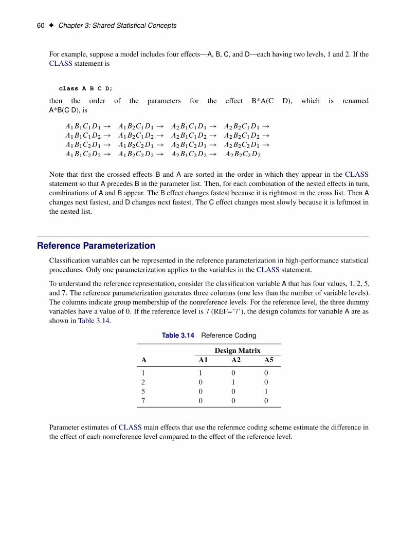
60 F Chapter 3: Shared Statistical Concepts
For example, suppose a model includes four effects—A, B, C, and D—each having two levels, 1 and 2. If theCLASS statement is
class A B C D;
then the order of the parameters for the effect B*A(C D), which is renamedA*B(C D), is
A1B1C1D1 ! A1B2C1D1 ! A2B1C1D1 ! A2B2C1D1 !
A1B1C1D2 ! A1B2C1D2 ! A2B1C1D2 ! A2B2C1D2 !
A1B1C2D1 ! A1B2C2D1 ! A2B1C2D1 ! A2B2C2D1 !
A1B1C2D2 ! A1B2C2D2 ! A2B1C2D2 ! A2B2C2D2
Note that first the crossed effects B and A are sorted in the order in which they appear in the CLASSstatement so that A precedes B in the parameter list. Then, for each combination of the nested effects in turn,combinations of A and B appear. The B effect changes fastest because it is rightmost in the cross list. Then Achanges next fastest, and D changes next fastest. The C effect changes most slowly because it is leftmost inthe nested list.
Reference ParameterizationClassification variables can be represented in the reference parameterization in high-performance statisticalprocedures. Only one parameterization applies to the variables in the CLASS statement.
To understand the reference representation, consider the classification variable A that has four values, 1, 2, 5,and 7. The reference parameterization generates three columns (one less than the number of variable levels).The columns indicate group membership of the nonreference levels. For the reference level, the three dummyvariables have a value of 0. If the reference level is 7 (REF=’7’), the design columns for variable A are asshown in Table 3.14.
Table 3.14 Reference Coding
Design MatrixA A1 A2 A5
1 1 0 0
2 0 1 0
5 0 0 1
7 0 0 0
Parameter estimates of CLASS main effects that use the reference coding scheme estimate the difference inthe effect of each nonreference level compared to the effect of the reference level.

Model Selection F 61
Model Selection
MethodsThe model selection methods implemented in high-performance statistical procedures are specified in theMETHOD= option in the SELECTION statement. The following methods are available, although specificprocedures might support only a subset of these methods. Furthermore, the examples in this section refer tofit criteria that might not be supported by a specific procedure.
Full Model Fitted
When METHOD=NONE, the complete model that is specified in the MODEL statement is used to fit themodel, and no effect selection is done.
Forward Selection
METHOD=FORWARD specifies the forward selection technique, which begins with just the intercept andthen sequentially adds the effect that most improves the fit. The process terminates when no significantimprovement can be obtained by adding any effect.
In the traditional implementation of forward selection, the statistic that is used to determine whether to addan effect is the significance level of a hypothesis test that reflects an effect’s contribution to the model if it isincluded. At each step, the effect that is most significant is added. The process stops when the significancelevel for adding any effect is greater than some specified entry significance level.
An alternative approach to address the critical problem of when to stop the selection process is to assess thequality of the models that are produced by the forward selection method and choose the model from thissequence that “best” balances goodness of fit against model complexity. You can use several criteria for thispurpose. These criteria fall into two groups—information criteria and criteria that are based on out-of-sampleprediction performance.
You use the CHOOSE= option to specify the criterion for selecting one model from the sequence of modelsproduced. If you do not specify a CHOOSE= criterion, then the model at the final step is the selected model.
For example, if you specify the following statement, then forward selection terminates at the step where noeffect can be added at the 0:2 significance level:
selection method=forward(select=SL choose=AIC SLE=0.2);
However, the selected model is the first one that has the minimum value of Akaike’s information criterion. Insome cases, this minimum value might occur at a step much earlier than the final step. In other cases, the AICmight start increasing only if more steps are performed—that is, a larger value is used for the significancelevel for entry. If you want to minimize AIC, then too many steps are performed in the former case and toofew in the latter case. To address this issue, high-performance statistical procedures enable you to specifya stopping criterion by using the STOP= option. When you specify a stopping criterion, forward selectioncontinues until a local extremum of the stopping criterion in the sequence of models generated is reached. Tobe deemed a local extremum, a criterion value at a given step must be better than its value at the next n steps,
62 F Chapter 3: Shared Statistical Concepts
where n is known as the “stop horizon.” By default, the stop horizon is three steps, but you can change thisby specifying the STOPHORIZON= option.
For example, if you specify the following statement, then forward selection terminates at the step wherethe effect to be added at the next step would produce a model that has an AIC statistic larger than the AICstatistic of the current model:
selection method=forward(select=SL stop=AIC) stophorizon=1;
In most cases, provided that the entry significance level is large enough that the local extremum of the namedcriterion occurs before the final step, specifying either of the following statements selects the same model,but more steps are done in the first case:
selection method=forward(select=SL choose=CRITERION);
selection method=forward(select=SL stop=CRITERION);
In some cases, there might be a better local extremum that cannot be reached if you specify the STOP= optionbut can be found if you use the CHOOSE= option. Also, you can use the CHOOSE= option in preference tothe STOP= option if you want to examine how the named criterion behaves as you move beyond the stepwhere the first local minimum of this criterion occurs.
You can specify both the CHOOSE= and STOP= options. You can also use these options together withoptions that specify size-based limits on the selected model. You might want to consider models that aregenerated by forward selection and have at most some fixed number of effects, but select from within this setbased on a criterion that you specify. For example, specifying the following statements requests that forwardselection continue until there are 20 effects in the final model and chooses among the sequence of models theone that has the largest value of the adjusted R-square statistic:
selection method=forward(stop=none maxeffects=20 choose=ADJRSQ);
You can also combine these options to select a model where one of two conditions is met. For example,the following statement chooses whatever occurs first between a local minimum of the sum of squares onvalidation data and a local minimum of the corrected Akaike’s information criterion (AICC):
selection method=forward(stop=AICC choose=VALIDATE);
It is important to keep in mind that forward selection bases the decision about what effect to add at anystep by considering models that differ by one effect from the current model. This search paradigm cannotguarantee reaching a “best” subset model. Furthermore, the add decision is greedy in the sense that the effectthat is deemed most significant is the effect that is added. However, if your goal is to find a model that is bestin terms of some selection criterion other than the significance level of the entering effect, then even thisone step choice might not be optimal. For example, the effect that you would add to get a model that hasthe smallest value of the Mallows’ C.p/ statistic at the next step is not necessarily the same effect that ismost significant based on a hypothesis test. High-performance statistical procedures enable you to specifythe criterion to optimize at each step by using the SELECT= option. For example, the following statementrequests that at each step the effect that is added be the one that produces a model that has the smallest valueof the Mallows’ C.p/ statistic:
Methods F 63
selection method=forward(select=CP);
In the case where all effects are variables (that is, effects with one degree of freedom and no hierarchy), usingADJRSQ, AIC, AICC, BIC, CP, RSQUARE, or SBC as the selection criterion for forward selection producesthe same sequence of additions. However, if the degrees of freedom contributed by different effects are notconstant or if an out-of-sample prediction-based criterion is used, then different sequences of additions mightbe obtained.
You can use the SELECT= option together with the CHOOSE= and STOP= options. If you specify only theSELECT= criterion, then this criterion is also used as the stopping criterion. In the previous example whereonly the selection criterion is specified, not only do effects enter based on the Mallows’ C.p/ statistic, butthe selection terminates when the C.p/ statistic has a local minimum.
You can find discussion and references to studies about criteria for variable selection in Burnham andAnderson (2002), along with some cautions and recommendations.
Examples of Forward Selection SpecificationsThe following statement adds effects that at each step produce the lowest value of the SBC statistic and stopsat the step where adding any effect would increase the SBC statistic:
selection method=forward stophorizon=1;
The following statement adds effects based on significance level and stops when all candidate effects forentry at a step have a significance level greater than the default entry significance level of 0.05:
selection=forward(select=SL);
The following statement adds effects based on significance level and stops at a step where adding any effectincreases the error sum of squares computed on the validation data:
selection=forward(select=SL stop=validation) stophorizon=1;
The following statement adds effects that at each step produce the lowest value of the AIC statistic and stopsat the first step whose AIC value is smaller than the AIC value at the next three steps:
selection=forward(select=AIC);
The following statement adds effects that at each step produce the largest value of the adjusted R-squarestatistic and stops at the step where the significance level that corresponds to the addition of this effect isgreater than 0.2:
selection=forward(select=ADJRSQ stop=SL SLE=0.2);
Backward Elimination
METHOD=BACKWARD specifies the backward elimination technique. This technique starts from the fullmodel, which includes all independent effects. Then effects are deleted one by one until a stopping conditionis satisfied. At each step, the effect that shows the smallest contribution to the model is deleted.

64 F Chapter 3: Shared Statistical Concepts
In the traditional implementation of backward selection, the statistic that is used to determine whether todrop an effect is significance level. At any step, the least significant predictor is dropped and the processcontinues until all effects that remain in the model are significant at a specified stay significance level (SLS).
Just as with forward selection, you can use the SELECT= option to change the criterion that is used to assesseffect contributions. You can also specify a stopping criterion in the STOP= option and use a CHOOSE=option to provide a criterion for selecting among the sequence of models produced. For more information,see the discussion in the section “Forward Selection” on page 61.
Examples of Backward Selection SpecificationsThe following statement removes effects that at each step produce the largest value of the Schwarz Bayesianinformation criterion (SBC) statistic and stops at the step where removing any effect increases the SBCstatistic:
selection method=backward stophorizon=1;
The following statement bases removal of effects on significance level and stops when all candidate effectsfor removal at a step are significant at the default stay significance level of 0.05:
selection method=backward(select=SL);
The following statement bases removal of effects on significance level and stops when all effects in the modelare significant at the 0:1 level. Finally, from the sequence of models generated, the chosen model is the onethat produces the smallest average square error when scored on the validation data:
selection method=backward(select=SL choose=validate SLS=0.1);
The following statement applies in logistic regression models the fast backward technique of Lawless andSinghal (1978), a first-order approximation that has greater numerical efficiency than full backward selection:
selection method=backward(fast);
The fast technique fits an initial full logistic model and a reduced model after the candidate effects have beendropped. On the other hand, full backward selection fits a logistic regression model each time an effect isremoved from the model.
Stepwise Selection
METHOD=STEPWISE specifies the stepwise method, which is a modification of the forward selectiontechnique that differs in that effects already in the model do not necessarily stay there.
In the traditional implementation of stepwise selection method, the same entry and removal significancelevels for the forward selection and backward elimination methods are used to assess contributions of effectsas they are added to or removed from a model. If, at a step of the stepwise method, any effect in the model isnot significant at the SLSTAY= level, then the least significant of these effects is removed from the model andthe algorithm proceeds to the next step. This ensures that no effect can be added to a model while some effectcurrently in the model is not deemed significant. Only after all necessary deletions have been accomplishedcan another effect be added to the model. In this case the effect whose addition is the most significant isadded to the model and the algorithm proceeds to the next step. The stepwise process ends when none of the
Methods F 65
effects outside the model is significant at the SLENTRY= level and every effect in the model is significant atthe SLSTAY= level. In some cases, neither of these two conditions for stopping is met and the sequence ofmodels cycles. In this case, the stepwise method terminates at the end of the cycle.
Just as you can in forward selection and backward elimination, you can use the SELECT= option to changethe criterion that is used to assess effect contributions. You can also use the STOP= option to specify astopping criterion and use a CHOOSE= option to provide a criterion for selecting among the sequence ofmodels produced. For more information, see the section “Forward Selection” on page 61.
For selection criteria other than significance level, high-performance statistical procedures optionally supporta further modification in the stepwise method. In the standard stepwise method, no effect can enter the modelif removing any effect currently in the model would yield an improved value of the selection criterion. In themodification, you can use the COMPETITIVE option to specify that addition and deletion of effects shouldbe treated competitively. The selection criterion is evaluated for all models that are produced by deletingan effect from the current model or by adding an effect to this model. The action that most improves theselection criterion is the action taken.
Examples of Stepwise Selection SpecificationsThe following statement requests stepwise selection based on the SBC criterion:
selection method=stepwise;
First, if removing any effect yields a model that has a lower SBC statistic than the current model, then theeffect that produces the smallest SBC statistic is removed. If removing any effect increases the SBC statistic,then provided that adding some effect lowers the SBC statistic, the effect that produces the model that has thelowest SBC is added.
The following statement requests the traditional stepwise method:
selection=stepwise(select=SL)
First, if the removal of any effect in the model is not significant at the default stay level of 0.05, then theleast significant effect is removed and the algorithm proceeds to the next step. Otherwise, the effect whoseaddition is the most significant is added, provided that it is significant at the default entry level of 0.05.
The following statement requests the traditional stepwise method, where effects enter and leave based onsignificance levels, but with the following extra check: if any effect to be added or removed yields a modelwhose SBC statistic is greater than the SBC statistic of the current model, then the stepwise method terminatesat the current model.
selection method=stepwise(select=SL stop=SBC) stophorizon=1;
In this case, the entry and stay significance levels still play a role because they determine whether an effect isdeleted from or added to the model. This extra check might result in the selection terminating before a localminimum of the SBC criterion is found.
The following statement selects effects to enter or drop as in the previous example except that the significancelevel for entry is now 0:1 and the significance level to stay is 0:08. From the sequence of models produced,the selected model is chosen to yield the minimum AIC statistic:
66 F Chapter 3: Shared Statistical Concepts
selection method=stepwise(select=SL SLE=0.1 SLS=0.08 choose=AIC);
The following statement requests stepwise selection that is based on the AICC criterion and treats additionsand deletions competitively:
selection method=stepwise(select=AICC competitive);
Each step evaluates the AICC statistics that correspond to the removal of any effect in the current modelor the addition of any effect to the current model and chooses the addition or removal that produced theminimum value, provided that this minimum is lower than the AICC statistic of the current model.
The following statement requests stepwise selection that is based on the SBC criterion, treats additions anddeletions competitively, and stops based on the average square error over the validation data:
selection=stepwise(select=SBC competitive stop=VALIDATE);
At any step, SBC statistics that correspond to the removal of any effect from the current model or the additionof any effect to the current model are evaluated. The addition or removal that produces the minimum SBCvalue is made. The average square error on the validation data for the model with this addition or removal isevaluated. The selection stops when the average square error so produced increases for three consecutivesteps.
Forward-Swap Selection
METHOD=FORWARDSWAP specifies the forward-swap selection method, which is an extension of theforward selection method. The forward-swap selection method incorporates steps that improve a model byreplacing an effect in the model with an effect that is not in the model. When the model selection criterion is Rsquare, this method is the same as the maximum R-square improvement (MAXR) method that is implementedin the REG procedure in SAS/STAT software. You cannot use the effect significance level as the selectioncriterion for the forward-swap method.
The forward-swap selection method begins by finding the one-effect model that produces the best value ofthe selection criterion. Then another effect (the one that yields the greatest improvement in the selectioncriterion) is added. After the two-effect model is obtained, each of the effects in the model is compared toeach effect that is not in the model. For each comparison, the forward-swap method determines whetherremoving one effect and replacing it with the other effect improves the selection criterion. After comparingall possible swaps, the forward-swap method makes the swap that produces the greatest improvement in theselection criterion. Comparisons begin again, and the process continues until the forward-swap method findsthat no other swap could improve the selection criterion. Thus, the two-variable model that is produced isconsidered the “best” two-variable model that the technique can find. Another variable is then added to themodel, and the comparing-and-swapping process is repeated to find the “best” three-variable model, and soon.
The difference between the stepwise selection method and the forward-swap selection method is that allswaps are evaluated before any addition is made in the forward-swap method. In the stepwise selectionmethod, the “worst” effect might be removed without considering what adding the “best” remaining effectsmight accomplish. Because the forward-swap method needs to examine all possible pairwise effect swaps ateach step of the selection process, the forward-swap method is much more computationally expensive thanthe stepwise selection method; it might not be appropriate for models that contain a large number of effects.

Methods F 67
Least Angle Regression
METHOD=LAR specifies least angle regression (LAR), which is supported in the HPREG procedure. LARwas introduced by Efron et al. (2004). Not only does this algorithm provide a selection method in its ownright, but with one additional modification, it can be used to efficiently produce LASSO solutions. Justlike the forward selection method, the LAR algorithm produces a sequence of regression models in whichone parameter is added at each step, terminating at the full least squares solution when all parameters haveentered the model.
The algorithm starts by centering the covariates and response and scaling the covariates so that they allhave the same corrected sum of squares. Initially all coefficients are zero, as is the predicted response. Thepredictor that is most correlated with the current residual is determined, and a step is taken in the direction ofthis predictor. The length of this step determines the coefficient of this predictor and is chosen so that someother predictor and the current predicted response have the same correlation with the current residual. At thispoint, the predicted response moves in the direction that is equiangular between these two predictors. Movingin this direction ensures that these two predictors continue to have a common correlation with the currentresidual. The predicted response moves in this direction until a third predictor has the same correlationwith the current residual as the two predictors already in the model. A new direction is determined that isequiangular among these three predictors, and the predicted response moves in this direction until a fourthpredictor, which has the same correlation with the current residual, joins the set. This process continues untilall predictors are in the model.
As in other selection methods, the issue of when to stop the selection process is crucial. You can use theCHOOSE= option to specify a criterion for choosing among the models at each step. You can also use theSTOP= option to specify a stopping criterion. These formulas use the approximation that at step k of theLAR algorithm, the model has k degrees of freedom. See Efron et al. (2004) for a detailed discussion of thisso-called simple approximation.
A modification of LAR selection that is suggested in Efron et al. (2004) uses the LAR algorithm to select theset of covariates in the model at any step, but it uses ordinary least squares regression with just these covariatesto obtain the regression coefficients. You can request this hybrid method by specifying the LSCOEFFSsuboption of METHOD=LAR.
Lasso Selection
Method=LASSO specifies the least absolute shrinkage and selection operator (LASSO) method, whichis supported in the HPREG procedure. LASSO arises from a constrained form of ordinary least squaresregression where the sum of the absolute values of the regression coefficients is constrained to be smallerthan a specified parameter. More precisely let X D .x1; x2; : : : ; xm/ denote the matrix of covariates andlet y denote the response, where the xis have been centered and scaled to have unit standard deviationand mean zero and y has mean zero. Then for a given parameter t , the LASSO regression coefficientsˇ D .ˇ1; ˇ2; : : : ; ˇm/ are the solution to the following constrained optimization problem:
minimizejjy �Xˇjj2 subject tomXjD1
jˇj j � t
Provided that the LASSO parameter t is small enough, some of the regression coefficients are exactly0. Hence, you can view the LASSO as selecting a subset of the regression coefficients for each LASSO
68 F Chapter 3: Shared Statistical Concepts
parameter. By increasing the LASSO parameter in discrete steps, you obtain a sequence of regressioncoefficients in which the nonzero coefficients at each step correspond to selected parameters.
Early implementations (Tibshirani 1996) of LASSO selection used quadratic programming techniques tosolve the constrained least squares problem for each LASSO parameter of interest. Later Osborne, Presnell,and Turlach (2000) developed a “homotopy method” that generates the LASSO solutions for all values of t .Efron et al. (2004) derived a variant of their algorithm for least angle regression that can be used to obtain asequence of LASSO solutions from which all other LASSO solutions can be obtained by linear interpolation.This algorithm for METHOD=LASSO is used in PROC HPREG. It can be viewed as a stepwise procedurewith a single addition to or deletion from the set of nonzero regression coefficients at any step.
As in the other selection methods that are supported by high-performance statistical procedures, you canuse the CHOOSE= option to specify a criterion to choose among the models at each step of the LASSOalgorithm. You can also use the STOP= option to specify a stopping criterion. For more information, seethe discussion in the section “Forward Selection” on page 61. The model degrees of freedom that PROCGLMSELECT uses at any step of the LASSO are simply the number of nonzero regression coefficients in themodel at that step. Efron et al. (2004) cite empirical evidence for doing this but do not give any mathematicaljustification for this choice.
A modification of LASSO selection suggested in Efron et al. (2004) uses the LASSO algorithm to select theset of covariates in the model at any step, but it uses ordinary least squares regression and just these covariatesto obtain the regression coefficients. You can request this hybrid method by specifying the LSCOEFFSsuboption of SELECTION=LASSO.
Adaptive Lasso Selection
Adaptive lasso selection is a modification of lasso selection; in adaptive lasso selection, weights are applied toeach of the parameters in forming the lasso constraint (Zou, 2006). More precisely, suppose that the responsey has mean 0 and the regressors x are scaled to have mean 0 and common standard deviation. Furthermore,suppose that you can find a suitable estimator O of the parameters in the true model and you define a weightvector by w D 1=j Oj , where � 0. Then the adaptive lasso regression coefficients ˇ D .ˇ1; ˇ2; : : : ; ˇm/are the solution to the following constrained optimization problem:
minimizejjy �Xˇjj2 subject tomXjD1
jwjˇj j � t
PROC HPREG uses the solution to the unconstrained least squares problem as the estimator O. This isappropriate unless collinearity is a concern. If the regressors are collinear or nearly collinear, then Zou (2006)suggests using a ridge regression estimate to form the adaptive weights.

References F 69
ReferencesBurnham, K. P., and Anderson, D. R. (2002), Model Selection and Multimodel Inference, Second Edition,New York: Springer-Verlag.
Efron, B., Hastie, T., Johnstone, I., and Tibshirani, R. (2004), “Least Angle Regression (with Discussion),”Annals of Statistics, 32, 407–499.
Lawless, J. F., and Singhal, K. (1978), “Efficient Screening of Nonnormal Regression Models,” Biometrics,34, 318–327.
Osborne, M., Presnell, B., and Turlach, B. (2000), “A New Approach to Variable Selection in Least SquaresProblems,” IMA Journal of Numerical Analysis, 20, 389–404.
Searle, S. R. (1971), Linear Models, New York: John Wiley & Sons.
Tibshirani, R. (1996), “Regression Shrinkage and Selection via the Lasso,” Journal of the Royal StatisticalSociety Series B, 58, 267–288.
Zou, H. (2006), “The Adaptive Lasso and Its Oracle Properties,” Journal of the American StatisticalAssociation, 101, 1418–1429.

70
Chapter 4
The HPGENSELECT Procedure
ContentsOverview: HPGENSELECT Procedure . . . . . . . . . . . . . . . . . . . . . . . . . . . . 72
PROC HPGENSELECT Features . . . . . . . . . . . . . . . . . . . . . . . . . . . . 72PROC HPGENSELECT Contrasted with PROC GENMOD . . . . . . . . . . . . . . 73
Getting Started: HPGENSELECT Procedure . . . . . . . . . . . . . . . . . . . . . . . . . 73Syntax: HPGENSELECT Procedure . . . . . . . . . . . . . . . . . . . . . . . . . . . . . . 79
PROC HPGENSELECT Statement . . . . . . . . . . . . . . . . . . . . . . . . . . . 79CLASS Statement . . . . . . . . . . . . . . . . . . . . . . . . . . . . . . . . . . . . 84CODE Statement . . . . . . . . . . . . . . . . . . . . . . . . . . . . . . . . . . . . . 85FREQ Statement . . . . . . . . . . . . . . . . . . . . . . . . . . . . . . . . . . . . . 85ID Statement . . . . . . . . . . . . . . . . . . . . . . . . . . . . . . . . . . . . . . . 86MODEL Statement . . . . . . . . . . . . . . . . . . . . . . . . . . . . . . . . . . . . 86OUTPUT Statement . . . . . . . . . . . . . . . . . . . . . . . . . . . . . . . . . . . 92PERFORMANCE Statement . . . . . . . . . . . . . . . . . . . . . . . . . . . . . . 94SELECTION Statement . . . . . . . . . . . . . . . . . . . . . . . . . . . . . . . . . 94WEIGHT Statement . . . . . . . . . . . . . . . . . . . . . . . . . . . . . . . . . . . 95ZEROMODEL Statement . . . . . . . . . . . . . . . . . . . . . . . . . . . . . . . . 96
Details: HPGENSELECT Procedure . . . . . . . . . . . . . . . . . . . . . . . . . . . . . . 97Missing Values . . . . . . . . . . . . . . . . . . . . . . . . . . . . . . . . . . . . . . 97Exponential Family Distributions . . . . . . . . . . . . . . . . . . . . . . . . . . . . 97Response Distributions . . . . . . . . . . . . . . . . . . . . . . . . . . . . . . . . . . 98Response Probability Distribution Functions . . . . . . . . . . . . . . . . . . . . . . 99Log-Likelihood Functions . . . . . . . . . . . . . . . . . . . . . . . . . . . . . . . . 102Computational Method: Multithreading . . . . . . . . . . . . . . . . . . . . . . . . . 106Choosing an Optimization Algorithm . . . . . . . . . . . . . . . . . . . . . . . . . . 107
First- or Second-Order Algorithms . . . . . . . . . . . . . . . . . . . . . . . 107Algorithm Descriptions . . . . . . . . . . . . . . . . . . . . . . . . . . . . . 109
Displayed Output . . . . . . . . . . . . . . . . . . . . . . . . . . . . . . . . . . . . . 111ODS Table Names . . . . . . . . . . . . . . . . . . . . . . . . . . . . . . . . . . . . 115
Examples: HPGENSELECT Procedure . . . . . . . . . . . . . . . . . . . . . . . . . . . . 116Example 4.1: Model Selection . . . . . . . . . . . . . . . . . . . . . . . . . . . . . 116Example 4.2: Modeling Binomial Data . . . . . . . . . . . . . . . . . . . . . . . . . 119Example 4.3: Tweedie Model . . . . . . . . . . . . . . . . . . . . . . . . . . . . . . 124
References . . . . . . . . . . . . . . . . . . . . . . . . . . . . . . . . . . . . . . . . . . . 126

72 F Chapter 4: The HPGENSELECT Procedure
Overview: HPGENSELECT ProcedureThe HPGENSELECT procedure is a high-performance procedure that provides model fitting and modelbuilding for generalized linear models. It fits models for standard distributions in the exponential family,such as the normal, Poisson, and Tweedie distributions. In addition, PROC HPGENSELECT fits multinomialmodels for ordinal and nominal responses, and it fits zero-inflated Poisson and negative binomial models forcount data. For all these models, the HPGENSELECT procedure provides forward, backward, and stepwisevariable selection.
PROC HPGENSELECT runs in either single-machine mode or distributed mode.
NOTE: Distributed mode requires SAS High-Performance Statistics.
PROC HPGENSELECT FeaturesThe HPGENSELECT procedure does the following:
• estimates the parameters of a generalized linear regression model by using maximum likelihoodtechniques
• provides model-building syntax in the CLASS statement and the effect-based MODEL statement,which are familiar from SAS/STAT procedures (in particular, the GLM, GENMOD, LOGISTIC,GLIMMIX, and MIXED procedures)
• enables you to split classification effects into individual components by using the SPLIT option in theCLASS statement
• permits any degree of interaction effects that involve classification and continuous variables
• provides multiple link functions
• provides models for zero-inflated count data
• provides cumulative link modeling for ordinal data and generalized logit modeling for unorderedmultinomial data
• enables model building (variable selection) through the SELECTION statement
• provides a WEIGHT statement for weighted analysis
• provides a FREQ statement for grouped analysis
• provides an OUTPUT statement to produce a data set that has predicted values and other observation-wise statistics
Because the HPGENSELECT procedure is a high-performance analytical procedure, it also does the follow-ing:
PROC HPGENSELECT Contrasted with PROC GENMOD F 73
• enables you to run in distributed mode on a cluster of machines that distribute the data and thecomputations
• enables you to run in single-machine mode on the server where SAS is installed
• exploits all the available cores and concurrent threads, regardless of execution mode
For more information, see the section “Processing Modes” on page 6 in Chapter 2, “Shared Concepts andTopics.”
PROC HPGENSELECT Contrasted with PROC GENMODThis section contrasts the HPGENSELECT procedure with the GENMOD procedure in SAS/STAT software.
The CLASS statement in the HPGENSELECT procedure permits two parameterizations: GLM parameter-ization and a reference parameterization. In contrast to the LOGISTIC, GENMOD, and other proceduresthat permit multiple parameterizations, the HPGENSELECT procedure does not mix parameterizationsacross the variables in the CLASS statement. In other words, all classification variables have the sameparameterization, and this parameterization is either GLM parameterization or reference parameterization.The CLASS statement also enables you to split an effect that involves a classification variable into multipleeffects that correspond to individual levels of the classification variable.
The default optimization technique used by the HPGENSELECT procedure is a modification of the Newton-Raphson algorithm with a ridged Hessian. You can choose different optimization techniques (includingfirst-order methods that do not require a crossproducts matrix or Hessian) by specifying the TECHNIQUE=option in the PROC HPGENSELECT statement.
As in the GENMOD procedure, the default parameterization of CLASS variables in the HPGENSELECTprocedure is GLM parameterization. You can change the parameterization by specifying the PARAM= optionin the CLASS statement.
The GENMOD procedure offers a wide variety of postfitting analyses, such as contrasts, estimates, tests ofmodel effects, and least squares means. The HPGENSELECT procedure is limited in postfitting functionalitybecause it is primarily designed for large-data tasks, such as predictive model building, model fitting, andscoring.
Getting Started: HPGENSELECT ProcedureThis example illustrates how you can use PROC HPGENSELECT to perform Poisson regression for countdata. The following DATA step contains 100 observations for a count response variable (Y), a continuousvariable (Total) to be used in a later analysis, and five categorical variables (C1–C5), each of which has fournumerical levels:
data getStarted;input C1-C5 Y Total;datalines;
0 3 1 1 3 2 28.361

74 F Chapter 4: The HPGENSELECT Procedure
2 3 0 3 1 2 39.8311 3 2 2 2 1 17.1331 2 0 0 3 2 12.7690 2 1 0 1 1 29.4640 2 1 0 2 1 4.1521 2 1 0 1 0 0.0000 2 1 1 2 1 20.1991 2 0 0 1 0 0.0000 1 1 3 3 2 53.3762 2 2 2 1 1 31.9230 3 2 0 3 2 37.9872 2 2 0 0 1 1.0820 2 0 2 0 1 6.3231 3 0 0 0 0 0.0001 2 1 2 3 2 4.2170 1 2 3 1 1 26.0841 1 0 0 1 0 0.0001 3 2 2 2 0 0.0002 1 3 1 1 2 52.6401 3 0 1 2 1 3.2572 0 2 3 0 5 88.0662 2 2 1 0 1 15.1963 1 3 1 0 1 11.9553 1 3 1 2 3 91.7903 1 1 2 3 7 232.4173 1 1 1 0 1 2.1243 1 0 0 0 2 32.7623 1 2 3 0 1 25.4152 2 0 1 2 1 42.7533 3 2 2 3 1 23.8542 0 0 2 3 2 49.4381 0 0 2 3 4 105.4490 0 2 3 0 6 101.5360 3 1 0 0 0 0.0003 0 1 0 1 1 5.9372 0 0 0 3 2 53.9521 0 1 0 3 2 23.6861 1 3 1 1 1 0.2872 1 3 0 3 7 281.5511 3 2 1 1 0 0.0002 1 0 0 1 0 0.0000 0 1 1 2 3 93.0090 1 0 1 0 2 25.0551 2 2 2 3 1 1.6910 3 2 3 1 1 10.7193 3 0 3 3 1 19.2792 0 0 2 1 2 40.8022 2 3 0 3 3 72.9240 2 0 3 0 1 10.2163 0 1 2 2 2 87.7732 1 2 3 1 0 0.0003 2 0 3 1 0 0.0003 0 3 0 0 2 62.0161 3 2 2 1 3 36.355
Getting Started: HPGENSELECT Procedure F 75
2 3 2 0 3 1 23.1901 0 1 2 1 1 11.7842 1 2 2 2 5 204.5273 0 1 1 2 5 115.9370 1 1 3 2 1 44.0282 2 1 3 1 4 52.2471 1 0 0 1 1 17.6213 3 1 2 1 2 10.7062 2 0 2 3 3 81.5060 1 0 0 2 2 81.8350 1 2 0 1 2 20.6473 2 2 2 0 1 3.1102 2 3 0 0 1 13.6791 2 2 3 2 1 6.4863 3 2 2 1 2 30.0250 0 3 1 3 6 202.1723 2 3 1 2 3 44.2210 3 0 0 0 1 27.6453 3 3 0 3 2 22.4702 3 2 0 2 0 0.0001 3 0 2 0 1 1.6281 3 1 0 2 0 0.0003 2 3 3 0 1 20.6843 1 0 2 0 4 108.0000 1 2 2 1 1 4.6150 2 3 2 2 1 12.4610 3 2 0 1 3 53.7982 1 1 2 0 1 36.3201 0 3 0 0 0 0.0000 0 3 2 0 1 19.9020 2 3 1 0 0 0.0002 2 2 1 3 2 31.8153 3 3 0 0 0 0.0002 2 1 3 3 2 17.9150 2 3 2 3 2 69.3151 3 1 2 1 0 0.0003 0 1 1 1 4 94.0502 1 1 1 3 6 242.2660 2 0 3 2 1 40.8852 0 1 1 2 2 74.7082 2 2 2 3 2 50.7341 0 2 2 1 3 35.9501 3 3 1 1 1 2.7773 1 2 1 3 5 118.0650 3 2 1 2 0 0.000;
The following statements fit a log-linked Poisson model to these data by using classification effects forvariables C1–C5:
proc hpgenselect data=getStarted;class C1-C5;model Y = C1-C5 / Distribution=Poisson Link=Log;
run;
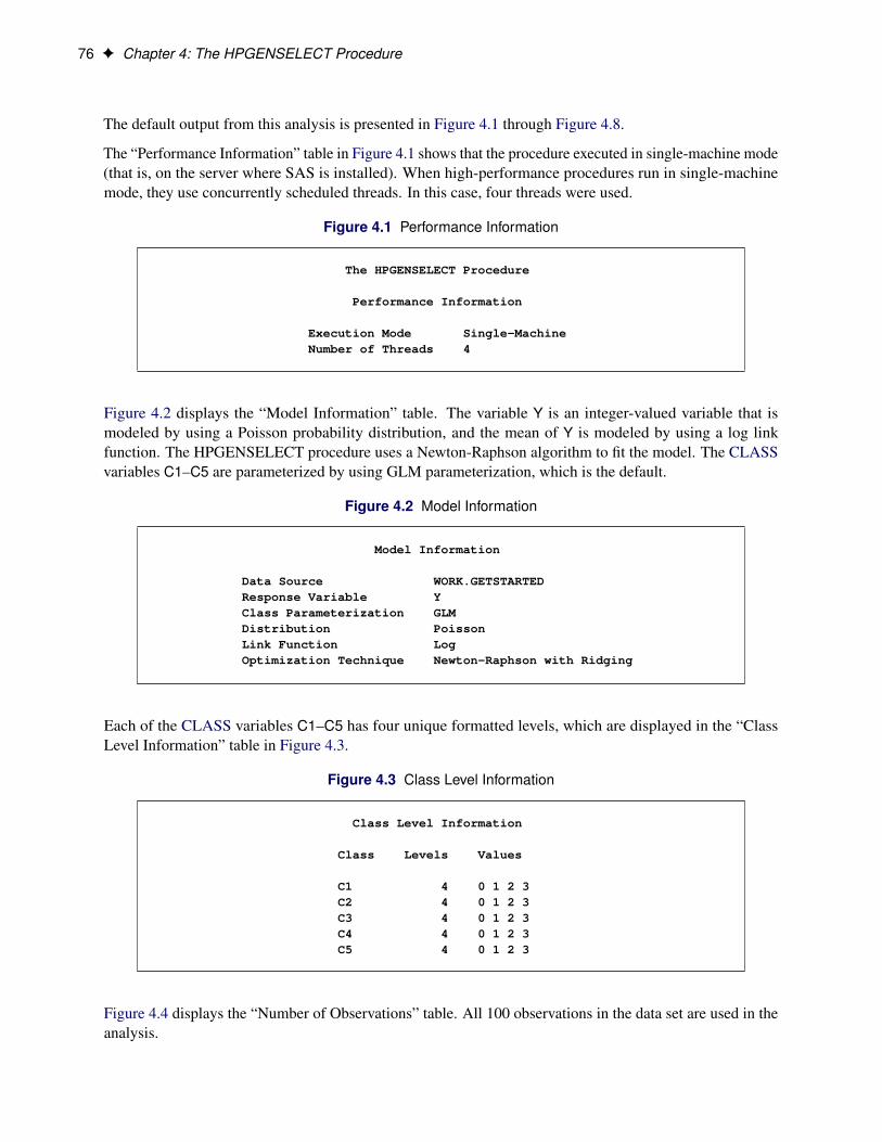
76 F Chapter 4: The HPGENSELECT Procedure
The default output from this analysis is presented in Figure 4.1 through Figure 4.8.
The “Performance Information” table in Figure 4.1 shows that the procedure executed in single-machine mode(that is, on the server where SAS is installed). When high-performance procedures run in single-machinemode, they use concurrently scheduled threads. In this case, four threads were used.
Figure 4.1 Performance Information
The HPGENSELECT Procedure
Performance Information
Execution Mode Single-MachineNumber of Threads 4
Figure 4.2 displays the “Model Information” table. The variable Y is an integer-valued variable that ismodeled by using a Poisson probability distribution, and the mean of Y is modeled by using a log linkfunction. The HPGENSELECT procedure uses a Newton-Raphson algorithm to fit the model. The CLASSvariables C1–C5 are parameterized by using GLM parameterization, which is the default.
Figure 4.2 Model Information
Model Information
Data Source WORK.GETSTARTEDResponse Variable YClass Parameterization GLMDistribution PoissonLink Function LogOptimization Technique Newton-Raphson with Ridging
Each of the CLASS variables C1–C5 has four unique formatted levels, which are displayed in the “ClassLevel Information” table in Figure 4.3.
Figure 4.3 Class Level Information
Class Level Information
Class Levels Values
C1 4 0 1 2 3C2 4 0 1 2 3C3 4 0 1 2 3C4 4 0 1 2 3C5 4 0 1 2 3
Figure 4.4 displays the “Number of Observations” table. All 100 observations in the data set are used in theanalysis.
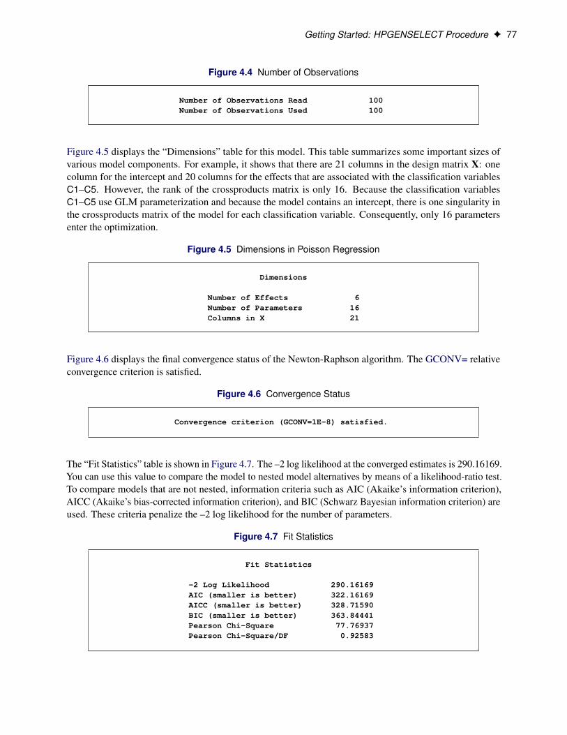
Getting Started: HPGENSELECT Procedure F 77
Figure 4.4 Number of Observations
Number of Observations Read 100Number of Observations Used 100
Figure 4.5 displays the “Dimensions” table for this model. This table summarizes some important sizes ofvarious model components. For example, it shows that there are 21 columns in the design matrix X: onecolumn for the intercept and 20 columns for the effects that are associated with the classification variablesC1–C5. However, the rank of the crossproducts matrix is only 16. Because the classification variablesC1–C5 use GLM parameterization and because the model contains an intercept, there is one singularity inthe crossproducts matrix of the model for each classification variable. Consequently, only 16 parametersenter the optimization.
Figure 4.5 Dimensions in Poisson Regression
Dimensions
Number of Effects 6Number of Parameters 16Columns in X 21
Figure 4.6 displays the final convergence status of the Newton-Raphson algorithm. The GCONV= relativeconvergence criterion is satisfied.
Figure 4.6 Convergence Status
Convergence criterion (GCONV=1E-8) satisfied.
The “Fit Statistics” table is shown in Figure 4.7. The –2 log likelihood at the converged estimates is 290.16169.You can use this value to compare the model to nested model alternatives by means of a likelihood-ratio test.To compare models that are not nested, information criteria such as AIC (Akaike’s information criterion),AICC (Akaike’s bias-corrected information criterion), and BIC (Schwarz Bayesian information criterion) areused. These criteria penalize the –2 log likelihood for the number of parameters.
Figure 4.7 Fit Statistics
Fit Statistics
-2 Log Likelihood 290.16169AIC (smaller is better) 322.16169AICC (smaller is better) 328.71590BIC (smaller is better) 363.84441Pearson Chi-Square 77.76937Pearson Chi-Square/DF 0.92583
78 F Chapter 4: The HPGENSELECT Procedure
The “Parameter Estimates” table in Figure 4.8 shows that many parameters have fairly large p-values,indicating that one or more of the model effects might not be necessary.
Figure 4.8 Parameter Estimates
Parameter Estimates
StandardParameter DF Estimate Error Chi-Square Pr > ChiSq
Intercept 1 0.881903 0.382730 5.3095 0.0212C1 0 1 -0.196002 0.211482 0.8590 0.3540C1 1 1 -0.605161 0.263508 5.2742 0.0216C1 2 1 -0.068458 0.210776 0.1055 0.7453C1 3 0 0 . . .C2 0 1 0.961117 0.255485 14.1521 0.0002C2 1 1 0.708188 0.246768 8.2360 0.0041C2 2 1 0.161741 0.266365 0.3687 0.5437C2 3 0 0 . . .C3 0 1 -0.227016 0.252561 0.8079 0.3687C3 1 1 -0.094775 0.229519 0.1705 0.6797C3 2 1 0.044801 0.238127 0.0354 0.8508C3 3 0 0 . . .C4 0 1 -0.280476 0.263589 1.1322 0.2873C4 1 1 0.028157 0.249652 0.0127 0.9102C4 2 1 0.047803 0.240378 0.0395 0.8424C4 3 0 0 . . .C5 0 1 -0.817936 0.219901 13.8351 0.0002C5 1 1 -0.710596 0.206265 11.8684 0.0006C5 2 1 -0.602080 0.217724 7.6471 0.0057C5 3 0 0 . . .

Syntax: HPGENSELECT Procedure F 79
Syntax: HPGENSELECT ProcedureThe following statements are available in the HPGENSELECT procedure:
PROC HPGENSELECT < options > ;CLASS variable < (options) >: : : < variable < (options) > > < / global-options > ;CODE < options > ;MODEL response< (response-options) > = < effects > < / model-options > ;MODEL events/trials< (response-options) > = < effects > < / model-options > ;OUTPUT < OUT=SAS-data-set >
< keyword < =name > >. . .< keyword < =name > > < / options > ;
PERFORMANCE performance-options ;SELECTION selection-options ;FREQ variable ;ID variables ;WEIGHT variable ;ZEROMODEL < effects >< / zeromodel-options > ;
The PROC HPGENSELECT statement and at least one MODEL statement are required. The CLASSstatement can appear multiple times. If a CLASS statement is specified, it must precede the MODELstatements.
PROC HPGENSELECT StatementPROC HPGENSELECT < options > ;
The PROC HPGENSELECT statement invokes the procedure. Table 4.1 summarizes the available options inthe PROC HPGENSELECT statement by function. The options are then described fully in alphabetical order.
Table 4.1 PROC HPGENSELECT Statement Options
Option Description
Basic OptionsALPHA= Specifies a global significance levelDATA= Specifies the input data setNAMELEN= Limits the length of effect names
Output OptionsCORR Displays the “Parameter Estimates Correlation Matrix” tableCOV Displays the “Parameter Estimates Covariance Matrix” tableITDETAILS Displays the “Iteration History” tableITSELECT Displays the “Iteration History” table when model selection is performedNOPRINT Suppresses ODS outputNOCLPRINT Limits or suppresses the display of classification variable levelsNOSTDERR Suppresses computation of the covariance matrix and standard errors
80 F Chapter 4: The HPGENSELECT Procedure
Table 4.1 continued
Option Description
Optimization OptionsABSCONV= Tunes the absolute function convergence criterionABSFCONV= Tunes the absolute function difference convergence criterionABSGCONV= Tunes the absolute gradient convergence criterionFCONV= Tunes the relative function difference convergence criterionGCONV= Tunes the relative gradient convergence criterionMAXITER= Chooses the maximum number of iterations in any optimizationMAXFUNC= Specifies the maximum number of function evaluations in any optimizationMAXTIME= Specifies the upper limit of CPU time (in seconds) for any optimizationMINITER= Specifies the minimum number of iterations in any optimizationNORMALIZE= Specifies whether the objective function is normalized during optimizationTECHNIQUE= Selects the optimization technique
Tolerance OptionsSINGCHOL= Tunes the singularity criterion for Cholesky decompositionsSINGSWEEP= Tunes the singularity criterion for the sweep operatorSINGULAR= Tunes the general singularity criterion
User-Defined Format OptionsFMTLIBXML= Specifies the file reference for a format stream
You can specify the following options in the PROC HPGENSELECT statement.
ABSCONV=r
ABSTOL=rspecifies an absolute function convergence criterion. For minimization, termination requires f . .k// �r, where is the vector of parameters in the optimization and f .�/ is the objective function. Thedefault value of r is the negative square root of the largest double-precision value, which serves only asa protection against overflow.
ABSFCONV=r < n >
ABSFTOL=r < n >specifies an absolute function difference convergence criterion. For all techniques except NMSIMP,termination requires a small change of the function value in successive iterations:
jf . .k�1// � f . .k//j � r
Here, denotes the vector of parameters that participate in the optimization, and f .�/ is the objectivefunction. The same formula is used for the NMSIMP technique, but .k/ is defined as the vertex thathas the lowest function value and .k�1/ is defined as the vertex that has the highest function value inthe simplex. The default value is r = 0. The optional integer value n specifies the number of successiveiterations for which the criterion must be satisfied before the process can be terminated.
PROC HPGENSELECT Statement F 81
ABSGCONV=r < n >
ABSGTOL=r < n >specifies an absolute gradient convergence criterion. Termination requires the maximum absolutegradient element to be small:
maxjjgj .
.k//j � r
Here, denotes the vector of parameters that participate in the optimization, and gj .�/ is the gradientof the objective function with respect to the j th parameter. This criterion is not used by the NMSIMPtechnique. The default value is r = 1E–8. The optional integer value n specifies the number ofsuccessive iterations for which the criterion must be satisfied before the process can be terminated.
ALPHA=numberspecifies a global significance level for the construction of confidence intervals. The confidence level is1 – number. The value of number must be between 0 and 1; the default is 0.05. You can override thisglobal significance level by specifying the ALPHA= option in the MODEL statement or the ALPHA=option in the OUTPUT statement.
CORRcreates the “Parameter Estimates Correlation Matrix” table. The correlation matrix is computed bynormalizing the covariance matrix†. That is, if �ij is an element of†, then the corresponding elementof the correlation matrix is �ij =�i�j , where �i D
p�i i .
COVcreates the “Parameter Estimates Covariance Matrix” table. The covariance matrix is computed as theinverse of the negative of the matrix of second derivatives of the log-likelihood function with respect tothe model parameters (the Hessian matrix).
DATA=SAS-data-setnames the input SAS data set for PROC HPGENSELECT to use. The default is the most recentlycreated data set.
If the procedure executes in distributed mode, the input data are distributed to memory on the appliancenodes and analyzed in parallel, unless the data are already distributed in the appliance database. Inthat case the procedure reads the data alongside the distributed database. For information about thevarious execution modes, see the section “Processing Modes” on page 6; for information about thealongside-the-database model, see the section “Alongside-the-Database Execution” on page 13.
FCONV=r < n >
FTOL=r < n >specifies a relative function difference convergence criterion. For all techniques except NMSIMP,termination requires a small relative change of the function value in successive iterations:
jf . .k// � f . .k�1//j
jf . .k�1//j� r
Here, denotes the vector of parameters that participate in the optimization, and f .�/ is the objectivefunction. The same formula is used for the NMSIMP technique, but .k/ is defined as the vertex thathas the lowest function value, and .k�1/ is defined as the vertex that has the highest function value inthe simplex.

82 F Chapter 4: The HPGENSELECT Procedure
The default value is r = 2 � �, where � is the machine precision. The optional integer value n specifiesthe number of successive iterations for which the criterion must be satisfied before the process canterminate.
FMTLIBXML=file-refspecifies the file reference for the XML stream that contains the user-defined format definitions. User-defined formats are handled differently in a distributed computing environment than they are in otherSAS products. For information about how to generate an XML stream for your formats, see the section“Working with Formats” on page 32 in Chapter 2, “Shared Concepts and Topics.”
GCONV=r < n >GTOL=r < n >
specifies a relative gradient convergence criterion. For all techniques except CONGRA and NMSIMP,termination requires that the normalized predicted function reduction be small:
g. .k//0ŒH.k/��1g. .k//jf . .k//j
� r
Here, denotes the vector of parameters that participate in the optimization, f .�/ is the objectivefunction, and g.�/ is the gradient. For the CONGRA technique (where a reliable Hessian estimate H isnot available), the following criterion is used:
k g. .k// k22 k s. .k// k2k g. .k// � g. .k�1// k2 jf . .k//j
� r
This criterion is not used by the NMSIMP technique. The default value is r=1E–8. The optional integervalue n specifies the number of successive iterations for which the criterion must be satisfied beforethe process can terminate.
ITDETAILSadds to the “Iteration History” table the current values of the parameter estimates and their gradients.These quantities are reported only for parameters that participate in the optimization. This option isnot available when you perform model selection.
ITSELECTgenerates the “Iteration History” table when you perform a model selection.
MAXFUNC=n
MAXFU=nspecifies the maximum number of function calls in the optimization process. The default values are asfollows, depending on the optimization technique:
• TRUREG, NRRIDG, NEWRAP: n = 125
• QUANEW, DBLDOG: n = 500
• CONGRA: n = 1,000
• NMSIMP: n = 3,000
The optimization can terminate only after completing a full iteration. Therefore, the number of functioncalls that are actually performed can exceed n. You can choose the optimization technique by specifyingthe TECHNIQUE= option.

PROC HPGENSELECT Statement F 83
MAXITER=n
MAXIT=nspecifies the maximum number of iterations in the optimization process. The default values are asfollows, depending on the optimization technique:
• TRUREG, NRRIDG, NEWRAP: n = 50
• QUANEW, DBLDOG: n = 200
• CONGRA: n = 400
• NMSIMP: n = 1,000
These default values also apply when n is specified as a missing value. You can choose the optimizationtechnique by specifying the TECHNIQUE= option.
MAXTIME=rspecifies an upper limit of r seconds of CPU time for the optimization process. The default value isthe largest floating-point double representation of your computer. The time specified by this option ischecked only once at the end of each iteration. Therefore, the actual running time can be longer than r.
MINITER=n
MINIT=nspecifies the minimum number of iterations. The default value is 0. If you request more iterations thanare actually needed for convergence to a stationary point, the optimization algorithms might behavestrangely. For example, the effect of rounding errors can prevent the algorithm from continuing for therequired number of iterations.
NAMELEN=numberspecifies the length to which long effect names are shortened. The default and minimum value is 20.
NOCLPRINT< =number >suppresses the display of the “Class Level Information” table if you do not specify number. If youspecify number, the values of the classification variables are displayed for only those variables whosenumber of levels is less than number. Specifying a number helps to reduce the size of the “Class LevelInformation” table if some classification variables have a large number of levels.
NOPRINTsuppresses the generation of ODS output.
NORMALIZE=YES | NOspecifies whether to normalize the objective function during optimization by the reciprocal of thefrequency count of observations that are used in the analysis. This option affects the values that arereported in the “Iteration History” table. The results that are reported in the “Fit Statistics” are alwaysdisplayed for the nonnormalized log-likelihood function. By default, NORMALIZE = NO.
NOSTDERRsuppresses the computation of the covariance matrix and the standard errors of the regression coef-ficients. When the model contains many variables (thousands), the inversion of the Hessian matrixto derive the covariance matrix and the standard errors of the regression coefficients can be time-consuming.
84 F Chapter 4: The HPGENSELECT Procedure
SINGCHOL=numbertunes the singularity criterion in Cholesky decompositions. The default is 1E4 times the machineepsilon; this product is approximately 1E–12 on most computers.
SINGSWEEP=numbertunes the singularity criterion for sweep operations. The default is 1E4 times the machine epsilon; thisproduct is approximately 1E–12 on most computers.
SINGULAR=numbertunes the general singularity criterion that is applied in sweeps and inversions. The default is 1E4 timesthe machine epsilon; this product is approximately 1E–12 on most computers.
TECHNIQUE=keyword
TECH=keywordspecifies the optimization technique for obtaining maximum likelihood estimates. You can choosefrom the following techniques by specifying the appropriate keyword :
CONGRA performs a conjugate-gradient optimization.
DBLDOG performs a version of double-dogleg optimization.
NEWRAP performs a Newton-Raphson optimization with line search.
NMSIMP performs a Nelder-Mead simplex optimization.
NONE performs no optimization.
NRRIDG performs a Newton-Raphson optimization with ridging.
QUANEW performs a dual quasi-Newton optimization.
TRUREG performs a trust-region optimization
The default value is TECHNIQUE=NRRIDG, except for the Tweedie distribution, for which the defaultvalue is TECHNIQUE=QUANEW.
For more information, see the section “Choosing an Optimization Algorithm” on page 107.
CLASS StatementCLASS variable < (options) >: : : < variable < (options) > > < / global-options > ;
The CLASS statement names the classification variables to be used as explanatory variables in the analysis.The CLASS statement must precede the MODEL statement. You can list the response variable for binary andmultinomial models in the CLASS statement, but this is not necessary.
The CLASS statement is documented in the section “CLASS Statement” on page 40 of Chapter 3, “SharedStatistical Concepts.”
The HPGENSELECT procedure additionally supports the following global-option in the CLASS statement:
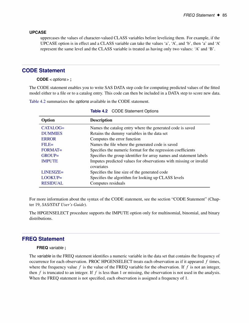
FREQ Statement F 85
UPCASEuppercases the values of character-valued CLASS variables before levelizing them. For example, if theUPCASE option is in effect and a CLASS variable can take the values ‘a’, ‘A’, and ‘b’, then ‘a’ and ‘A’represent the same level and the CLASS variable is treated as having only two values: ‘A’ and ‘B’.
CODE StatementCODE < options > ;
The CODE statement enables you to write SAS DATA step code for computing predicted values of the fittedmodel either to a file or to a catalog entry. This code can then be included in a DATA step to score new data.
Table 4.2 summarizes the options available in the CODE statement.
Table 4.2 CODE Statement Options
Option Description
CATALOG= Names the catalog entry where the generated code is savedDUMMIES Retains the dummy variables in the data setERROR Computes the error functionFILE= Names the file where the generated code is savedFORMAT= Specifies the numeric format for the regression coefficientsGROUP= Specifies the group identifier for array names and statement labelsIMPUTE Imputes predicted values for observations with missing or invalid
covariatesLINESIZE= Specifies the line size of the generated codeLOOKUP= Specifies the algorithm for looking up CLASS levelsRESIDUAL Computes residuals
For more information about the syntax of the CODE statement, see the section “CODE Statement” (Chap-ter 19, SAS/STAT User’s Guide).
The HPGENSELECT procedure supports the IMPUTE option only for multinomial, binomial, and binarydistributions.
FREQ StatementFREQ variable ;
The variable in the FREQ statement identifies a numeric variable in the data set that contains the frequency ofoccurrence for each observation. PROC HPGENSELECT treats each observation as if it appeared f times,where the frequency value f is the value of the FREQ variable for the observation. If f is not an integer,then f is truncated to an integer. If f is less than 1 or missing, the observation is not used in the analysis.When the FREQ statement is not specified, each observation is assigned a frequency of 1.
86 F Chapter 4: The HPGENSELECT Procedure
ID StatementID variables ;
The ID statement lists one or more variables from the input data set that are to be transferred to the outputdata set that is specified in the OUTPUT statement.
For more information, see the section “ID Statement” on page 44 in Chapter 3, “Shared Statistical Concepts.”
MODEL StatementMODEL response < (response-options) > = < effects > < / model-options > ;
MODEL events / trials = < effects > < / model-options > ;
The MODEL statement defines the statistical model in terms of a response variable (the target) or anevents/trials specification. You can also specify model effects that are constructed from variables in the inputdata set, and you can specify options. An intercept is included in the model by default. You can remove theintercept by specifying the NOINT option.
You can specify a single response variable that contains your interval, binary, ordinal, or nominal responsevalues. When you have binomial data, you can specify the events/trials form of the response, where onevariable contains the number of positive responses (or events) and another variable contains the number oftrials. The values of both events and (trials – events) must be nonnegative, and the value of trials must bepositive. If you specify a single response variable that is in a CLASS statement, then the response is assumedto be either binary or multinomial, depending on the number of levels.
For information about constructing the model effects, see the section “Specification and Parameterization ofModel Effects” on page 52 of Chapter 3, “Shared Statistical Concepts.”
There are two sets of options in the MODEL statement. The response-options determine how theHPGENSELECT procedure models probabilities for binary and multinomial data. The model-optionscontrol other aspects of model formation and inference. Table 4.3 summarizes these options.
Table 4.3 MODEL Statement Options
Option Description
Response Variable Options for Binary and Multinomial ModelsDESCENDING Reverses the response categoriesEVENT= Specifies the event categoryORDER= Specifies the sort orderREF= Specifies the reference category
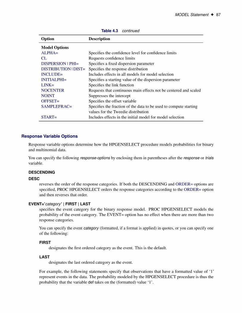
MODEL Statement F 87
Table 4.3 continued
Option Description
Model OptionsALPHA= Specifies the confidence level for confidence limitsCL Requests confidence limitsDISPERSION | PHI= Specifies a fixed dispersion parameterDISTRIBUTION | DIST= Specifies the response distributionINCLUDE= Includes effects in all models for model selectionINITIALPHI= Specifies a starting value of the dispersion parameterLINK= Specifies the link functionNOCENTER Requests that continuous main effects not be centered and scaledNOINT Suppresses the interceptOFFSET= Specifies the offset variableSAMPLEFRAC= Specifies the fraction of the data to be used to compute starting
values for the Tweedie distributionSTART= Includes effects in the initial model for model selection
Response Variable Options
Response variable options determine how the HPGENSELECT procedure models probabilities for binaryand multinomial data.
You can specify the following response-options by enclosing them in parentheses after the response or trialsvariable.
DESCENDING
DESCreverses the order of the response categories. If both the DESCENDING and ORDER= options arespecified, PROC HPGENSELECT orders the response categories according to the ORDER= optionand then reverses that order.
EVENT=’category ’ | FIRST | LASTspecifies the event category for the binary response model. PROC HPGENSELECT models theprobability of the event category. The EVENT= option has no effect when there are more than tworesponse categories.
You can specify the event category (formatted, if a format is applied) in quotes, or you can specify oneof the following:
FIRSTdesignates the first ordered category as the event. This is the default.
LASTdesignates the last ordered category as the event.
For example, the following statements specify that observations that have a formatted value of ‘1’represent events in the data. The probability modeled by the HPGENSELECT procedure is thus theprobability that the variable def takes on the (formatted) value ‘1’.
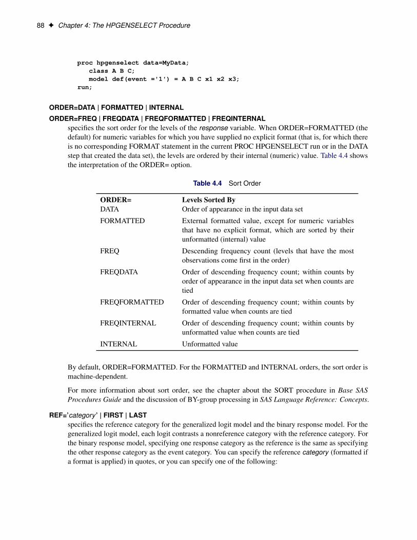
88 F Chapter 4: The HPGENSELECT Procedure
proc hpgenselect data=MyData;class A B C;model def(event ='1') = A B C x1 x2 x3;
run;
ORDER=DATA | FORMATTED | INTERNAL
ORDER=FREQ | FREQDATA | FREQFORMATTED | FREQINTERNALspecifies the sort order for the levels of the response variable. When ORDER=FORMATTED (thedefault) for numeric variables for which you have supplied no explicit format (that is, for which thereis no corresponding FORMAT statement in the current PROC HPGENSELECT run or in the DATAstep that created the data set), the levels are ordered by their internal (numeric) value. Table 4.4 showsthe interpretation of the ORDER= option.
Table 4.4 Sort Order
ORDER= Levels Sorted ByDATA Order of appearance in the input data set
FORMATTED External formatted value, except for numeric variablesthat have no explicit format, which are sorted by theirunformatted (internal) value
FREQ Descending frequency count (levels that have the mostobservations come first in the order)
FREQDATA Order of descending frequency count; within counts byorder of appearance in the input data set when counts aretied
FREQFORMATTED Order of descending frequency count; within counts byformatted value when counts are tied
FREQINTERNAL Order of descending frequency count; within counts byunformatted value when counts are tied
INTERNAL Unformatted value
By default, ORDER=FORMATTED. For the FORMATTED and INTERNAL orders, the sort order ismachine-dependent.
For more information about sort order, see the chapter about the SORT procedure in Base SASProcedures Guide and the discussion of BY-group processing in SAS Language Reference: Concepts.
REF=’category ’ | FIRST | LASTspecifies the reference category for the generalized logit model and the binary response model. For thegeneralized logit model, each logit contrasts a nonreference category with the reference category. Forthe binary response model, specifying one response category as the reference is the same as specifyingthe other response category as the event category. You can specify the reference category (formatted ifa format is applied) in quotes, or you can specify one of the following:
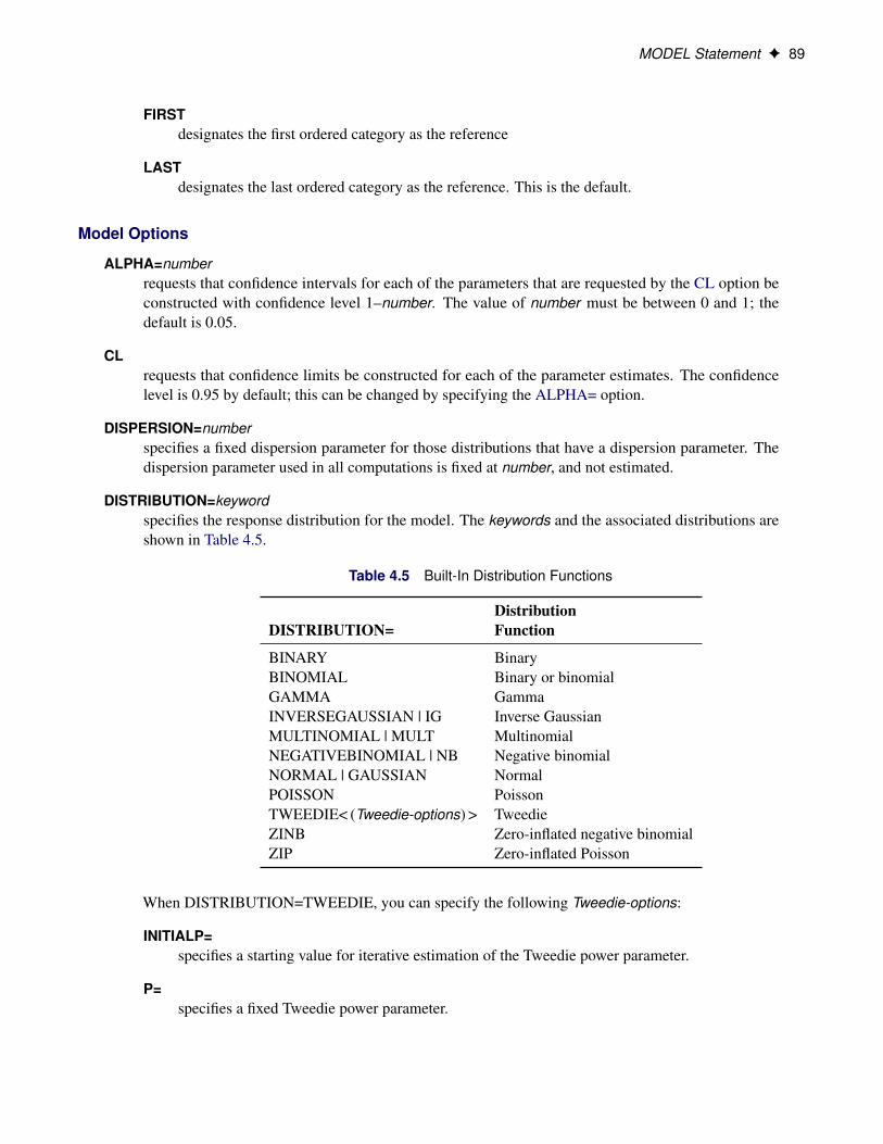
MODEL Statement F 89
FIRSTdesignates the first ordered category as the reference
LASTdesignates the last ordered category as the reference. This is the default.
Model Options
ALPHA=numberrequests that confidence intervals for each of the parameters that are requested by the CL option beconstructed with confidence level 1–number. The value of number must be between 0 and 1; thedefault is 0.05.
CLrequests that confidence limits be constructed for each of the parameter estimates. The confidencelevel is 0.95 by default; this can be changed by specifying the ALPHA= option.
DISPERSION=numberspecifies a fixed dispersion parameter for those distributions that have a dispersion parameter. Thedispersion parameter used in all computations is fixed at number, and not estimated.
DISTRIBUTION=keywordspecifies the response distribution for the model. The keywords and the associated distributions areshown in Table 4.5.
Table 4.5 Built-In Distribution Functions
DistributionDISTRIBUTION= Function
BINARY BinaryBINOMIAL Binary or binomialGAMMA GammaINVERSEGAUSSIAN | IG Inverse GaussianMULTINOMIAL | MULT MultinomialNEGATIVEBINOMIAL | NB Negative binomialNORMAL | GAUSSIAN NormalPOISSON PoissonTWEEDIE< (Tweedie-options) > TweedieZINB Zero-inflated negative binomialZIP Zero-inflated Poisson
When DISTRIBUTION=TWEEDIE, you can specify the following Tweedie-options:
INITIALP=specifies a starting value for iterative estimation of the Tweedie power parameter.
P=specifies a fixed Tweedie power parameter.
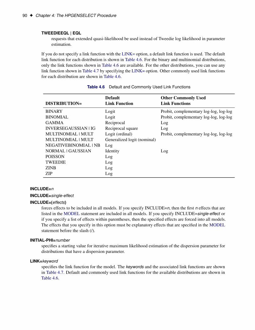
90 F Chapter 4: The HPGENSELECT Procedure
TWEEDIEEQL | EQLrequests that extended quasi-likelihood be used instead of Tweedie log likelihood in parameterestimation.
If you do not specify a link function with the LINK= option, a default link function is used. The defaultlink function for each distribution is shown in Table 4.6. For the binary and multinomial distributions,only the link functions shown in Table 4.6 are available. For the other distributions, you can use anylink function shown in Table 4.7 by specifying the LINK= option. Other commonly used link functionsfor each distribution are shown in Table 4.6.
Table 4.6 Default and Commonly Used Link Functions
Default Other Commonly UsedDISTRIBUTION= Link Function Link Functions
BINARY Logit Probit, complementary log-log, log-logBINOMIAL Logit Probit, complementary log-log, log-logGAMMA Reciprocal LogINVERSEGAUSSIAN | IG Reciprocal square LogMULTINOMIAL | MULT Logit (ordinal) Probit, complementary log-log, log-logMULTINOMIAL | MULT Generalized logit (nominal)NEGATIVEBINOMIAL | NB LogNORMAL | GAUSSIAN Identity LogPOISSON LogTWEEDIE LogZINB LogZIP Log
INCLUDE=n
INCLUDE=single-effect
INCLUDE=(effects)forces effects to be included in all models. If you specify INCLUDE=n, then the first n effects that arelisted in the MODEL statement are included in all models. If you specify INCLUDE=single-effect orif you specify a list of effects within parentheses, then the specified effects are forced into all models.The effects that you specify in this option must be explanatory effects that are specified in the MODELstatement before the slash (/).
INITIAL-PHI=numberspecifies a starting value for iterative maximum likelihood estimation of the dispersion parameter fordistributions that have a dispersion parameter.
LINK=keywordspecifies the link function for the model. The keywords and the associated link functions are shownin Table 4.7. Default and commonly used link functions for the available distributions are shown inTable 4.6.
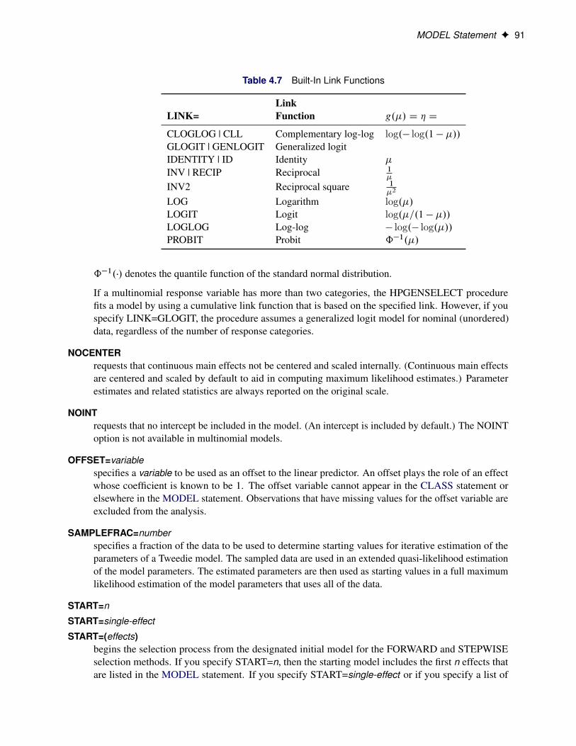
MODEL Statement F 91
Table 4.7 Built-In Link Functions
LinkLINK= Function g.�/ D � D
CLOGLOG | CLL Complementary log-log log.� log.1 � �//GLOGIT | GENLOGIT Generalized logitIDENTITY | ID Identity �
INV | RECIP Reciprocal 1�
INV2 Reciprocal square 1�2
LOG Logarithm log.�/LOGIT Logit log.�=.1 � �//LOGLOG Log-log � log.� log.�//PROBIT Probit ˆ�1.�/
ˆ�1.�/ denotes the quantile function of the standard normal distribution.
If a multinomial response variable has more than two categories, the HPGENSELECT procedurefits a model by using a cumulative link function that is based on the specified link. However, if youspecify LINK=GLOGIT, the procedure assumes a generalized logit model for nominal (unordered)data, regardless of the number of response categories.
NOCENTERrequests that continuous main effects not be centered and scaled internally. (Continuous main effectsare centered and scaled by default to aid in computing maximum likelihood estimates.) Parameterestimates and related statistics are always reported on the original scale.
NOINTrequests that no intercept be included in the model. (An intercept is included by default.) The NOINToption is not available in multinomial models.
OFFSET=variablespecifies a variable to be used as an offset to the linear predictor. An offset plays the role of an effectwhose coefficient is known to be 1. The offset variable cannot appear in the CLASS statement orelsewhere in the MODEL statement. Observations that have missing values for the offset variable areexcluded from the analysis.
SAMPLEFRAC=numberspecifies a fraction of the data to be used to determine starting values for iterative estimation of theparameters of a Tweedie model. The sampled data are used in an extended quasi-likelihood estimationof the model parameters. The estimated parameters are then used as starting values in a full maximumlikelihood estimation of the model parameters that uses all of the data.
START=n
START=single-effect
START=(effects)begins the selection process from the designated initial model for the FORWARD and STEPWISEselection methods. If you specify START=n, then the starting model includes the first n effects thatare listed in the MODEL statement. If you specify START=single-effect or if you specify a list of
92 F Chapter 4: The HPGENSELECT Procedure
effects within parentheses, then the starting model includes those specified effects. The effects that youspecify in the START= option must be explanatory effects that are specified in the MODEL statementbefore the slash (/). The START= option is not available when you specify METHOD=BACKWARDin the SELECTION statement.
OUTPUT StatementOUTPUT < OUT=SAS-data-set >
< keyword < =name > >. . . < keyword < =name > > < / options > ;
The OUTPUT statement creates a data set that contains observationwise statistics that are computed afterthe model is fitted. The variables in the input data set are not included in the output data set to avoid dataduplication for large data sets; however, variables that are specified in the ID statement are included.
If the input data are in distributed form, where accessing data in a particular order cannot be guaranteed, theHPGENSELECT procedure copies the distribution or partition key to the output data set so that its contentscan be joined with the input data.
The computation of the output statistics is based on the final parameter estimates. If the model fit does notconverge, missing values are produced for the quantities that depend on the estimates.
When there are more than two response levels for multinomial data, values are computed only for variablesthat are named by the XBETA and PREDICTED keywords; the other variables have missing values. Thesestatistics are computed for every response category, and the automatic variable _LEVEL_ identifies theresponse category on which the computed values are based. If you also specify the OBSCAT option, then theobservationwise statistics are computed only for the observed response category, as indicated by the value ofthe _LEVEL_ variable.
For observations in which only the response variable is missing, values of the XBETA and PREDICTEDstatistics are computed even though these observations do not affect the model fit. For zero-inflated models,ZBETA and PZERO are also computed. This practice enables predicted mean values or predicted probabilitiesto be computed for new observations.
You can specify the following syntax elements in the OUTPUT statement before the slash (/).
OUT=SAS-data-set
DATA=SAS-data-setspecifies the name of the output data set. If the OUT= (or DATA=) option is omitted, the procedureuses the DATAn convention to name the output data set.
keyword < =name >specifies a statistic to include in the output data set and optionally assigns a name to the variable. Ifyou do not provide a name, the HPGENSELECT procedure assigns a default name based on the typeof statistic requested.
You can specify the following keywords for adding statistics to the OUTPUT data set:
ADJPEARSON | ADJPEARS | STDRESCHIrequests the Pearson residual, adjusted to have unit variance. The adjusted Pearson residualis defined for the ith observation as yi��ip
�V.�i /.1�hi /, where V.�/ is the response distribution
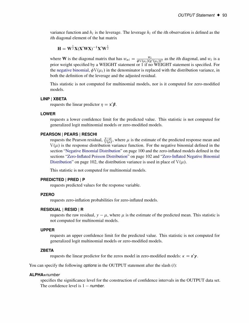
OUTPUT Statement F 93
variance function and hi is the leverage. The leverage hi of the ith observation is defined as theith diagonal element of the hat matrix
H DW12X.X0WX/�1X0W
12
where W is the diagonal matrix that has wei D wi�V.�i /.g 0.�i //2
as the ith diagonal, and wi is aprior weight specified by a WEIGHT statement or 1 if no WEIGHT statement is specified. Forthe negative binomial, �V.�i / in the denominator is replaced with the distribution variance, inboth the definition of the leverage and the adjusted residual.
This statistic is not computed for multinomial models, nor is it computed for zero-modifiedmodels.
LINP | XBETArequests the linear predictor � D x0ˇ.
LOWERrequests a lower confidence limit for the predicted value. This statistic is not computed forgeneralized logit multinomial models or zero-modified models.
PEARSON | PEARS | RESCHIrequests the Pearson residual, y��V.�/ , where � is the estimate of the predicted response mean andV.�/ is the response distribution variance function. For the negative binomial defined in thesection “Negative Binomial Distribution” on page 100 and the zero-inflated models defined in thesections “Zero-Inflated Poisson Distribution” on page 102 and “Zero-Inflated Negative BinomialDistribution” on page 102, the distribution variance is used in place of V.�/.
This statistic is not computed for multinomial models.
PREDICTED | PRED | Prequests predicted values for the response variable.
PZEROrequests zero-inflation probabilities for zero-inflated models.
RESIDUAL | RESID | Rrequests the raw residual, y � �, where � is the estimate of the predicted mean. This statistic isnot computed for multinomial models.
UPPERrequests an upper confidence limit for the predicted value. This statistic is not computed forgeneralized logit multinomial models or zero-modified models.
ZBETArequests the linear predictor for the zeros model in zero-modified models: � D z0 .
You can specify the following options in the OUTPUT statement after the slash (/):
ALPHA=numberspecifies the significance level for the construction of confidence intervals in the OUTPUT data set.The confidence level is 1 � number.
94 F Chapter 4: The HPGENSELECT Procedure
OBSCATrequests (for multinomial models) that observationwise statistics be produced only for the responselevel. If the OBSCAT option is not specified and the response variable has J levels, then the followingoutputs are created: for cumulative link models, J � 1 records are output for every observation inthe input data that corresponds to the J � 1 lower-ordered response categories; for generalized logitmodels, J records are output that correspond to all J response categories.
PERFORMANCE StatementPERFORMANCE < performance-options > ;
You can use the PERFORMANCE statement to control whether the procedure executes in single-machine ordistributed mode. The default is single-machine mode.
You can also use this statement to define performance parameters for multithreaded and distributed computing,and you can request details about performance results.
The PERFORMANCE statement is documented in the section “PERFORMANCE Statement” on page 34 ofChapter 2, “Shared Concepts and Topics.”
SELECTION StatementSELECTION < options > ;
The SELECTION statement performs model selection by examining whether effects should be added to orremoved from the model according to rules that are defined by model selection methods. The statementis fully documented in the section “SELECTION Statement” on page 45 in Chapter 3, “Shared StatisticalConcepts.”
The HPGENSELECT procedure supports the following effect-selection methods in the SELECTION state-ment:
METHOD=NONE results in no model selection. This method fits the full model.
METHOD=FORWARD performs forward selection. This method starts with no effects in themodel and adds effects.
METHOD=BACKWARD performs backward elimination. This method starts with all effects in themodel and deletes effects.
METHOD=STEPWISE performs stepwise regression. This method is similar to the FORWARDmethod except that effects already in the model do not necessarily staythere.
The only effect-selection criterion supported by the HPGENSELECT procedure is SELECT=SL, whereeffects enter and leave the model based on an evaluation of the significance level. To determine this level ofsignificance for each candidate effect, the HPGENSELECT procedure calculates an approximate chi-squaretest statistic.
The following criteria are available for the CHOOSE= option in the SELECT statement:
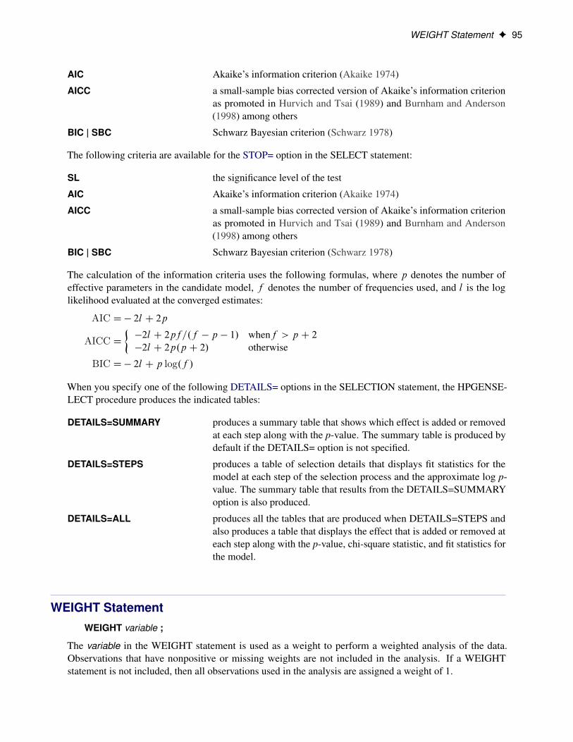
WEIGHT Statement F 95
AIC Akaike’s information criterion (Akaike 1974)
AICC a small-sample bias corrected version of Akaike’s information criterionas promoted in Hurvich and Tsai (1989) and Burnham and Anderson(1998) among others
BIC | SBC Schwarz Bayesian criterion (Schwarz 1978)
The following criteria are available for the STOP= option in the SELECT statement:
SL the significance level of the test
AIC Akaike’s information criterion (Akaike 1974)
AICC a small-sample bias corrected version of Akaike’s information criterionas promoted in Hurvich and Tsai (1989) and Burnham and Anderson(1998) among others
BIC | SBC Schwarz Bayesian criterion (Schwarz 1978)
The calculation of the information criteria uses the following formulas, where p denotes the number ofeffective parameters in the candidate model, f denotes the number of frequencies used, and l is the loglikelihood evaluated at the converged estimates:
AIC D� 2l C 2p
AICC D��2l C 2pf=.f � p � 1/ whenf > p C 2
�2l C 2p.p C 2/ otherwise
BIC D� 2l C p log.f /
When you specify one of the following DETAILS= options in the SELECTION statement, the HPGENSE-LECT procedure produces the indicated tables:
DETAILS=SUMMARY produces a summary table that shows which effect is added or removedat each step along with the p-value. The summary table is produced bydefault if the DETAILS= option is not specified.
DETAILS=STEPS produces a table of selection details that displays fit statistics for themodel at each step of the selection process and the approximate log p-value. The summary table that results from the DETAILS=SUMMARYoption is also produced.
DETAILS=ALL produces all the tables that are produced when DETAILS=STEPS andalso produces a table that displays the effect that is added or removed ateach step along with the p-value, chi-square statistic, and fit statistics forthe model.
WEIGHT StatementWEIGHT variable ;
The variable in the WEIGHT statement is used as a weight to perform a weighted analysis of the data.Observations that have nonpositive or missing weights are not included in the analysis. If a WEIGHTstatement is not included, then all observations used in the analysis are assigned a weight of 1.
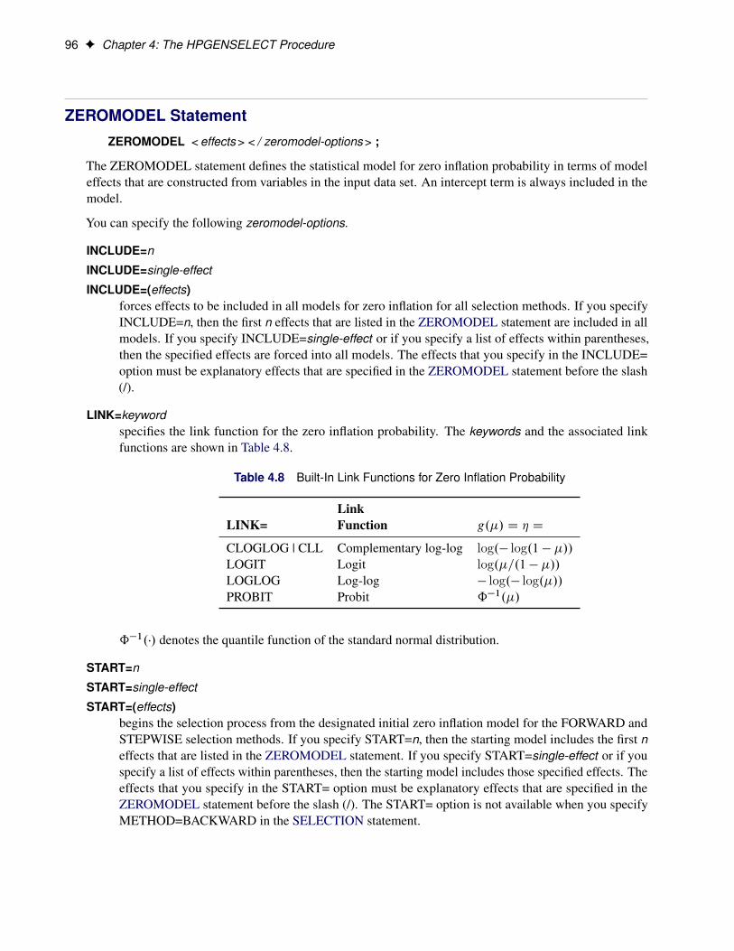
96 F Chapter 4: The HPGENSELECT Procedure
ZEROMODEL StatementZEROMODEL < effects > < / zeromodel-options > ;
The ZEROMODEL statement defines the statistical model for zero inflation probability in terms of modeleffects that are constructed from variables in the input data set. An intercept term is always included in themodel.
You can specify the following zeromodel-options.
INCLUDE=n
INCLUDE=single-effect
INCLUDE=(effects)forces effects to be included in all models for zero inflation for all selection methods. If you specifyINCLUDE=n, then the first n effects that are listed in the ZEROMODEL statement are included in allmodels. If you specify INCLUDE=single-effect or if you specify a list of effects within parentheses,then the specified effects are forced into all models. The effects that you specify in the INCLUDE=option must be explanatory effects that are specified in the ZEROMODEL statement before the slash(/).
LINK=keywordspecifies the link function for the zero inflation probability. The keywords and the associated linkfunctions are shown in Table 4.8.
Table 4.8 Built-In Link Functions for Zero Inflation Probability
LinkLINK= Function g.�/ D � D
CLOGLOG | CLL Complementary log-log log.� log.1 � �//LOGIT Logit log.�=.1 � �//LOGLOG Log-log � log.� log.�//PROBIT Probit ˆ�1.�/
ˆ�1.�/ denotes the quantile function of the standard normal distribution.
START=n
START=single-effect
START=(effects)begins the selection process from the designated initial zero inflation model for the FORWARD andSTEPWISE selection methods. If you specify START=n, then the starting model includes the first neffects that are listed in the ZEROMODEL statement. If you specify START=single-effect or if youspecify a list of effects within parentheses, then the starting model includes those specified effects. Theeffects that you specify in the START= option must be explanatory effects that are specified in theZEROMODEL statement before the slash (/). The START= option is not available when you specifyMETHOD=BACKWARD in the SELECTION statement.

Details: HPGENSELECT Procedure F 97
Details: HPGENSELECT Procedure
Missing ValuesAny observation that has missing values for the response, frequency, weight, offset, or explanatory variablesis excluded from the analysis; however, missing values are valid for response and explanatory variables thatare specified in the MISSING option in the CLASS statement. Observations that have a nonpositive weightor a frequency less than 1 are also excluded.
The estimated linear predictor and the fitted probabilities are not computed for any observation that hasmissing offset or explanatory variable values. However, if only the response value is missing, the linearpredictor and the fitted probabilities can be computed and output to a data set by using the OUTPUTstatement.
Exponential Family DistributionsMany of the probability distributions that the HPGENSELECT procedure fits are members of an exponentialfamily of distributions, which have probability distributions that are expressed as follows for some functionsb and c that determine the specific distribution:
f .y/ D exp�y� � b.�/
�C c.y; �/
�For fixed �, this is a one-parameter exponential family of distributions. The response variable can be discreteor continuous, so f .y/ represents either a probability mass function or a probability density function. Amore useful parameterization of generalized linear models is by the mean and variance of the distribution:
E.Y / D b0.�/
Var.Y / D b00.�/�
In generalized linear models, the mean of the response distribution is related to linear regression parametersthrough a link function,
g.�i / D x0iˇ
for the ith observation, where xi is a fixed known vector of explanatory variables and ˇ is a vector ofregression parameters. The HPGENSELECT procedure parameterizes models in terms of the regressionparameters ˇ and either the dispersion parameter � or a parameter that is related to �, depending on themodel. For exponential family models, the distribution variance is Var.Y / D �V.�/ where V.�/ is avariance function that depends only on �.
The zero-inflated models and the multinomial models are not exponential family models, but they are closelyrelated models that are useful and are included in the HPGENSELECT procedure.

98 F Chapter 4: The HPGENSELECT Procedure
Response DistributionsThe response distribution is the probability distribution of the response (target) variable. The HPGENSELECTprocedure can fit data for the following distributions:
• binary distribution
• binomial distribution
• gamma distribution
• inverse Gaussian distribution
• multinomial distribution (ordinal and nominal)
• negative binomial distribution
• normal (Gaussian) distribution
• Poisson distribution
• Tweedie distribution
• zero-inflated negative binomial distribution
• zero-inflated Poisson distribution
Expressions for the probability distributions (probability density functions for continuous variables orprobability mass functions for discrete variables) are shown in the section “Response Probability DistributionFunctions” on page 99. The expressions for the log-likelihood functions of these distributions are given inthe section “Log-Likelihood Functions” on page 102.
The binary (or Bernoulli) distribution is the elementary distribution of a discrete random variable that cantake on two values that have probabilities p and 1 � p. Suppose the random variable is denoted Y and
Pr.Y D 1/ D pPr.Y D 0/ D 1 � p
The value that is associated with probability p is often termed the event or “success”; the complementaryevent is termed the non-event or “failure.” A Bernoulli experiment is a random draw from a binary distributionand generates events with probability p.
If Y1; � � � ; Yn are n independent Bernoulli random variables, then their sum follows a binomial distribution.In other words, if Yi D 1 denotes an event (success) in the i th Bernoulli trial, a binomial random variableis the number of events (successes) in n independent Bernoulli trials. If you use the events/trials syntax inthe MODEL statement and you specify the DISTRIBUTION=BINOMIAL option, the HPGENSELECTprocedure fits the model as if the data had arisen from a binomial distribution. For example, the followingstatements fit a binomial regression model that has regressors x1 and x2. The variables e and t represent theevents and trials, respectively, for the binomial distribution:
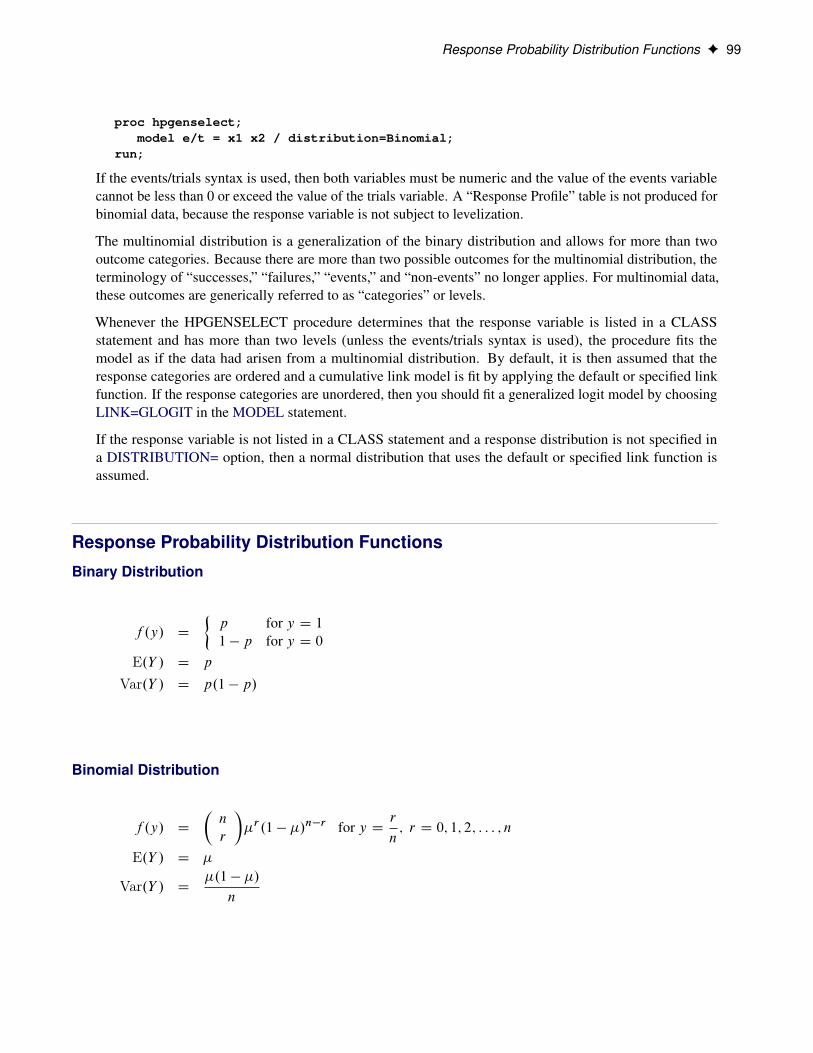
Response Probability Distribution Functions F 99
proc hpgenselect;model e/t = x1 x2 / distribution=Binomial;
run;
If the events/trials syntax is used, then both variables must be numeric and the value of the events variablecannot be less than 0 or exceed the value of the trials variable. A “Response Profile” table is not produced forbinomial data, because the response variable is not subject to levelization.
The multinomial distribution is a generalization of the binary distribution and allows for more than twooutcome categories. Because there are more than two possible outcomes for the multinomial distribution, theterminology of “successes,” “failures,” “events,” and “non-events” no longer applies. For multinomial data,these outcomes are generically referred to as “categories” or levels.
Whenever the HPGENSELECT procedure determines that the response variable is listed in a CLASSstatement and has more than two levels (unless the events/trials syntax is used), the procedure fits themodel as if the data had arisen from a multinomial distribution. By default, it is then assumed that theresponse categories are ordered and a cumulative link model is fit by applying the default or specified linkfunction. If the response categories are unordered, then you should fit a generalized logit model by choosingLINK=GLOGIT in the MODEL statement.
If the response variable is not listed in a CLASS statement and a response distribution is not specified ina DISTRIBUTION= option, then a normal distribution that uses the default or specified link function isassumed.
Response Probability Distribution Functions
Binary Distribution
f .y/ D
�p for y D 11 � p for y D 0
E.Y / D p
Var.Y / D p.1 � p/
Binomial Distribution
f .y/ D
�n
r
��r.1 � �/n�r for y D
r
n; r D 0; 1; 2; : : : ; n
E.Y / D �
Var.Y / D�.1 � �/
n

100 F Chapter 4: The HPGENSELECT Procedure
Gamma Distribution
f .y/ D1
�.�/y
�y�
�
��exp
��y�
�
�for 0 < y <1
� D1
�E.Y / D �
Var.Y / D�2
�
For the gamma distribution, � D 1�
is the estimated dispersion parameter that is displayed in the output. Theparameter � is also sometimes called the gamma index parameter.
Inverse Gaussian Distribution
f .y/ D1p
2�y3�exp
"�1
2y
�y � �
��
�2#for 0 < y <1
� D �2
Var.Y / D ��3
Multinomial Distribution
f .y1; y2; � � � ; yk/ DmŠ
y1Šy2Š � � �ykŠpy11 p
y22 � � �p
ykk
Negative Binomial Distribution
f .y/ D�.y C 1=k/
�.y C 1/�.1=k/
.k�/y
.1C k�/yC1=kfor y D 0; 1; 2; : : :
� D k
E.Y / D �
Var.Y / D �C ��2
For the negative binomial distribution, k is the estimated dispersion parameter that is displayed in the output.

Response Probability Distribution Functions F 101
Normal Distribution
f .y/ D1
p2��
exp��1
2
�y � ��
�2�for �1 < y <1
� D �2
E.Y / D �
Var.Y / D �
Poisson Distribution
f .y/ D�ye��
yŠfor y D 0; 1; 2; : : :
E.Y / D �
Var.Y / D �
Tweedie Distribution
The Tweedie model is a generalized linear model from the exponential family. The Tweedie distribution ischaracterized by three parameters: the mean parameter �, the dispersion �, and the power p. The varianceof the distribution is ��p. For values of p in the range 1 < p < 2, a Tweedie random variable can berepresented as a Poisson sum of gamma distributed random variables. That is,
Y D
NXiD1
Yi
where N has a Poisson distribution that has mean � D �2�p
�.2�p/and the Yi s have independent, identical
gamma distributions, each of which has an expected value E.Yi / D �.2 � p/�p�1 and an index parameter�i D
2�pp�1
.
In this case, Y has a discrete mass at 0, Pr.Y D 0/ D Pr.N D 0/ D exp.��/, and the probability densityof Y f .y/ is represented by an infinite series for y > 0. The HPGENSELECT procedure restricts thepower parameter to satisfy 1:1 <D p for numerical stability in model fitting. The Tweedie distribution doesnot have a general closed form representation for all values of p. It can be characterized in terms of thedistribution mean parameter �, dispersion parameter �, and power parameter p. For more information aboutthe Tweedie distribution, see Frees (2010).
The distribution mean and variance are given by:
E.Y / D �
Var.Y / D ��p
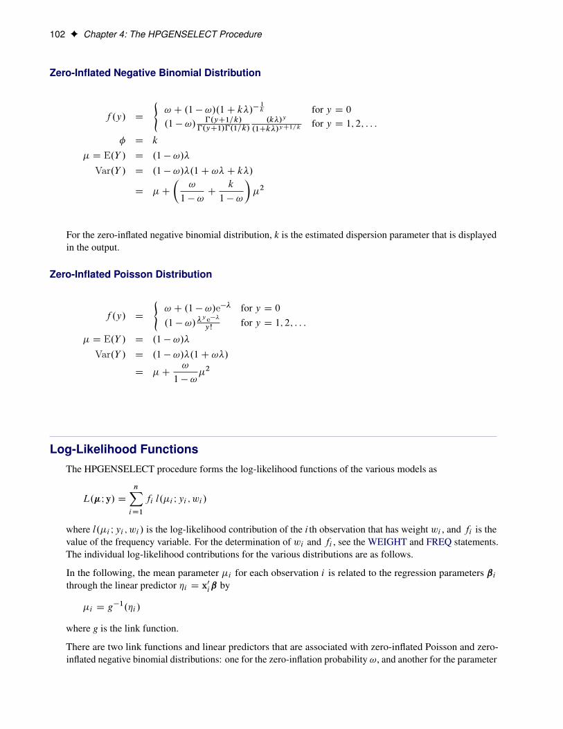
102 F Chapter 4: The HPGENSELECT Procedure
Zero-Inflated Negative Binomial Distribution
f .y/ D
(! C .1 � !/.1C k�/�
1k for y D 0
.1 � !/ �.yC1=k/�.yC1/�.1=k/
.k�/y
.1Ck�/yC1=kfor y D 1; 2; : : :
� D k
� D E.Y / D .1 � !/�
Var.Y / D .1 � !/�.1C !�C k�/
D �C
�!
1 � !C
k
1 � !
��2
For the zero-inflated negative binomial distribution, k is the estimated dispersion parameter that is displayedin the output.
Zero-Inflated Poisson Distribution
f .y/ D
(! C .1 � !/e�� for y D 0.1 � !/�
ye��yŠ
for y D 1; 2; : : :
� D E.Y / D .1 � !/�
Var.Y / D .1 � !/�.1C !�/
D �C!
1 � !�2
Log-Likelihood FunctionsThe HPGENSELECT procedure forms the log-likelihood functions of the various models as
L.�I y/ DnXiD1
fi l.�i Iyi ; wi /
where l.�i Iyi ; wi / is the log-likelihood contribution of the i th observation that has weight wi , and fi is thevalue of the frequency variable. For the determination of wi and fi , see the WEIGHT and FREQ statements.The individual log-likelihood contributions for the various distributions are as follows.
In the following, the mean parameter �i for each observation i is related to the regression parameters ˇithrough the linear predictor �i D x0iˇ by
�i D g�1.�i /
where g is the link function.
There are two link functions and linear predictors that are associated with zero-inflated Poisson and zero-inflated negative binomial distributions: one for the zero-inflation probability !, and another for the parameter
Log-Likelihood Functions F 103
�, which is the Poisson or negative binomial mean if there is no zero-inflation. Each of these parameters isrelated to regression parameters through an individual link function,
�i D x0iˇ�i D z0i
�i .ˇ/ D g�1.�i /
!i . / D h�1.�i /
where h is one of the following link functions that are associated with binary data: complementary log-log,log-log, logit, or probit. These link functions are also shown in Table 4.8.
Binary Distribution
The HPGENSELECT procedure computes the log-likelihood function l.�i .ˇ/Iyi / for the i th binary obser-vation as
�i D x0iˇ
�i .ˇ/ D g�1.�i /
l.�i .ˇ/Iyi / D yi logf�ig C .1 � yi / logf1 � �ig
Here, �i is the probability of an event, and the variable yi takes on the value 1 for an event and the value 0for a non-event. The inverse link function g�1.�/ maps from the scale of the linear predictor �i to the scale ofthe mean. For example, for the logit link (the default),
�i .ˇ/ Dexpf�ig
1C expf�ig
You can control which binary outcome in your data is modeled as the event by specifying the response-options in the MODEL statement, and you can choose the link function by specifying the LINK= option inthe MODEL statement.
If a WEIGHT statement is specified and wi denotes the weight for the current observation, the log-likelihoodfunction is computed as
l.�i .ˇ/Iyi ; wi / D wi l.�i .ˇ/Iyi /
Binomial Distribution
The HPGENSELECT procedure computes the log-likelihood function l.�i .ˇ/Iyi / for the i th binomialobservation as
�i D x0iˇ
�i .ˇ/ D g�1.�i /
l.�i .ˇ/Iyi ; wi / D wi .yi logf�ig C .ni � yi / logf1 � �ig/C wi .logf�.ni C 1/g � logf�.yi C 1/g � logf�.ni � yi C 1/g/
where yi and ni are the values of the events and trials of the i th observation, respectively. �i measuresthe probability of events (successes) in the underlying Bernoulli distribution whose aggregate follows thebinomial distribution.
104 F Chapter 4: The HPGENSELECT Procedure
Gamma Distribution
The HPGENSELECT procedure computes the log-likelihood function l.�i .ˇ/Iyi / for the i th observation as
�i D x0iˇ
�i .ˇ/ D g�1.�i /
l.�i .ˇ/Iyi ; wi / Dwi
�log
�wiyi
��i
��wiyi
��i� log.yi / � log
��
�wi
�
��For the gamma distribution, � D 1
�is the estimated dispersion parameter that is displayed in the output.
Inverse Gaussian Distribution
The HPGENSELECT procedure computes the log-likelihood function l.�i .ˇ/Iyi / for the i th observation as
�i D x0iˇ
�i .ˇ/ D g�1.�i /
l.�i .ˇ/Iyi ; wi / D �1
2
"wi .yi � �i /
2
yi�2�C log
�y3iwi
!C log.2�/
#
where � is the dispersion parameter.
Multinomial Distribution
The multinomial distribution that is modeled by the HPGENSELECT procedure is a generalization of thebinary distribution; it is the distribution of a single draw from a discrete distribution with J possible values.The log-likelihood function for the i th observation is
l.�i I yi ; wi / D wiJXjD1
yij logf�ij g
In this expression, J denotes the number of response categories (the number of possible outcomes) and �ijis the probability that the i th observation takes on the response value that is associated with category j . Thecategory probabilities must satisfy
JXjD1
�j D 1
and the constraint is satisfied by modeling J � 1 categories. In models that have ordered response categories,the probabilities are expressed in cumulative form, so that the last category is redundant. In generalizedlogit models (multinomial models that have unordered categories), one category is chosen as the referencecategory and the linear predictor in the reference category is set to 0.
Log-Likelihood Functions F 105
Negative Binomial Distribution
The HPGENSELECT procedure computes the log-likelihood function l.�i .ˇ/Iyi / for the i th observation as
�i D x0iˇ
�i .ˇ/ D g�1.�i /
l.�i .ˇ/Iyi ; wi / D yi log�k�
wi
�� .yi C wi=k/ log
�1C
k�
wi
�C log
��.yi C wi=k/
�.yi C 1/�.wi=k/
�where k is the negative binomial dispersion parameter that is displayed in the output.
Normal Distribution
The HPGENSELECT procedure computes the log-likelihood function l.�i .ˇ/Iyi / for the i th observation as
�i D x0iˇ
�i .ˇ/ D g�1.�i /
l.�i .ˇ/Iyi ; wi / D �1
2
�wi .yi � �i /
2
�C log
��
wi
�C log.2�/
�where � is the dispersion parameter.
Poisson Distribution
The HPGENSELECT procedure computes the log-likelihood function l.�i .ˇ/Iyi / for the i th observation as
�i D x0iˇ
�i .ˇ/ D g�1.�i /
l.�i .ˇ/Iyi ; wi / D wi Œyi log.�i / � �i � log.yi Š/�
Tweedie Distribution
The Tweedie distribution does not in general have a closed form log-likelihood function in terms of the mean,dispersion, and power parameters. The form of the log-likelihood is
L.�I y/ DnXiD1
fi l.�i Iyi ; wi /
where
l.�i ; yi ; wi / D log.f .yi I�i ; p;�
wi//
and f .y; �; p; �/ is the Tweedie probability distribution, which is described in the section “Tweedie Distri-bution” on page 101. Evaluation of the Tweedie log-likelihood for model fitting is performed numerically asdescribed in Dunn and Smyth (2005, 2008).

106 F Chapter 4: The HPGENSELECT Procedure
Zero-Inflated Negative Binomial Distribution
The HPGENSELECT procedure computes the log-likelihood function l.�i .ˇ/; !i . /Iyi / for the i th obser-vation as
�i D x0iˇ�i D z0i
�i .ˇ/ D g�1.�i /
!i . / D h�1.�i /
l.�i .ˇ/; !i . /Iyi ; wi / D
8ˆ<ˆ:
logŒ!i C .1 � !i /.1C kwi�/�
1k � yi D 0
log.1 � !i /C yi log�k�wi
��.yi C
wik/ log
�1C k�
wi
�C log
��.yiC
wik/
�.yiC1/�.wik/
�yi > 0
where k is the zero-inflated negative binomial dispersion parameter that is displayed in the output.
Zero-Inflated Poisson Distribution
The HPGENSELECT procedure computes the log-likelihood function l.�i .ˇ/; !i . /Iyi / for the i th obser-vation as
�i D x0iˇ�i D z0i
�i .ˇ/ D g�1.�i /
!i . / D h�1.�i /
l.�i .ˇ/; !i . /Iyi ; wi / D
8<:wi logŒ!i C .1 � !i / exp.��i /� yi D 0
wi Œlog.1 � !i /C yi log.�i / � �i � log.yi Š/� yi > 0
Computational Method: MultithreadingThreading refers to the organization of computational work into multiple tasks (processing units that canbe scheduled by the operating system). A task is associated with a thread. Multithreading refers to theconcurrent execution of threads. When multithreading is possible, substantial performance gains can berealized compared to sequential (single-threaded) execution.
The number of threads spawned by the HPGENSELECT procedure is determined by the number of CPUs ona machine and can be controlled in the following ways:
• You can specify the number of CPUs in the CPUCOUNT= SAS system option. For example, if youspecify the following statement, the HPGENSELECT procedure determines threading as if it executedon a system that has four CPUs, regardless of the actual CPU count:

Choosing an Optimization Algorithm F 107
options cpucount=4;
• You can specify the NTHREADS= option in the PERFORMANCE statement to control the number ofthreads. This specification overrides the CPUCOUNT= system option. Specify NTHREADS=1 toforce single-threaded execution.
The number of threads per machine is displayed in the “Dimensions” table, which is part of the default output.The HPGENSELECT procedure allocates one thread per CPU by default.
The tasks that are multithreaded by the HPGENSELECT procedure are primarily defined by dividing thedata that are processed on a single machine among the threads—that is, the HPGENSELECT procedureimplements multithreading through a data-parallel model. For example, if the input data set has 1,000observations and PROC HPGENSELECT is running with four threads, then 250 observations are associatedwith each thread. All operations that require access to the data are then multithreaded. These operationsinclude the following:
• variable levelization
• effect levelization
• formation of the initial crossproducts matrix
• formation of approximate Hessian matrices for candidate evaluation during model selection
• objective function calculation
• gradient calculation
• Hessian calculation
• scoring of observations
In addition, operations on matrices such as sweeps can be multithreaded provided that the matrices areof sufficient size to realize performance benefits from managing multiple threads for the particular matrixoperation.
Choosing an Optimization Algorithm
First- or Second-Order Algorithms
The factors that affect how you choose an optimization technique for a particular problem are complex.Although the default method works well for most problems, you might occasionally benefit from tryingseveral different algorithms.
For many optimization problems, computing the gradient takes more computer time than computing thefunction value. Computing the Hessian sometimes takes much more computer time and memory thancomputing the gradient, especially when there are many decision variables. Unfortunately, optimizationtechniques that do not use some kind of Hessian approximation usually require many more iterations thantechniques that do use a Hessian matrix; as a result, the total run time of these techniques is often longer.
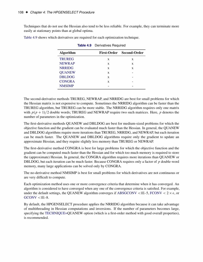
108 F Chapter 4: The HPGENSELECT Procedure
Techniques that do not use the Hessian also tend to be less reliable. For example, they can terminate moreeasily at stationary points than at global optima.
Table 4.9 shows which derivatives are required for each optimization technique.
Table 4.9 Derivatives Required
Algorithm First-Order Second-Order
TRUREG x xNEWRAP x xNRRIDG x xQUANEW x -DBLDOG x -CONGRA x -NMSIMP - -
The second-derivative methods TRUREG, NEWRAP, and NRRIDG are best for small problems for whichthe Hessian matrix is not expensive to compute. Sometimes the NRRIDG algorithm can be faster than theTRUREG algorithm, but TRUREG can be more stable. The NRRIDG algorithm requires only one matrixwith p.p C 1/=2 double words; TRUREG and NEWRAP require two such matrices. Here, p denotes thenumber of parameters in the optimization.
The first-derivative methods QUANEW and DBLDOG are best for medium-sized problems for which theobjective function and the gradient can be evaluated much faster than the Hessian. In general, the QUANEWand DBLDOG algorithms require more iterations than TRUREG, NRRIDG, and NEWRAP, but each iterationcan be much faster. The QUANEW and DBLDOG algorithms require only the gradient to update anapproximate Hessian, and they require slightly less memory than TRUREG or NEWRAP.
The first-derivative method CONGRA is best for large problems for which the objective function and thegradient can be computed much faster than the Hessian and for which too much memory is required to storethe (approximate) Hessian. In general, the CONGRA algorithm requires more iterations than QUANEW orDBLDOG, but each iteration can be much faster. Because CONGRA requires only a factor of p double-wordmemory, many large applications can be solved only by CONGRA.
The no-derivative method NMSIMP is best for small problems for which derivatives are not continuous orare very difficult to compute.
Each optimization method uses one or more convergence criteria that determine when it has converged. Analgorithm is considered to have converged when any one of the convergence criteria is satisfied. For example,under the default settings, the QUANEW algorithm converges if ABSGCONV <1E–5, FCONV < 2 � �, orGCONV <1E–8.
By default, the HPGENSELECT procedure applies the NRRIDG algorithm because it can take advantageof multithreading in Hessian computations and inversions. If the number of parameters becomes large,specifying the TECHNIQUE=QUANEW option (which is a first-order method with good overall properties),is recommended.

Choosing an Optimization Algorithm F 109
Algorithm Descriptions
The following subsections provide details about each optimization technique and follow the same order asTable 4.9.
Trust Region Optimization (TRUREG)The trust region method uses the gradient g. .k// and the Hessian matrix H. .k//; thus, it requires that theobjective function f . / have continuous first- and second-order derivatives inside the feasible region.
The trust region method iteratively optimizes a quadratic approximation to the nonlinear objective functionwithin a hyperelliptic trust region with radius � that constrains the step size that corresponds to the quality ofthe quadratic approximation. The trust region method is implemented based on Dennis, Gay, and Welsch(1981); Gay (1983); Moré and Sorensen (1983).
The trust region method performs well for small- to medium-sized problems, and it does not need manyfunction, gradient, and Hessian calls. However, if the computation of the Hessian matrix is computationallyexpensive, one of the dual quasi-Newton or conjugate gradient algorithms might be more efficient.
Newton-Raphson Optimization with Line Search (NEWRAP)The NEWRAP technique uses the gradient g. .k// and the Hessian matrix H. .k//; thus, it requires that theobjective function have continuous first- and second-order derivatives inside the feasible region.
If second-order derivatives are computed efficiently and precisely, the NEWRAP method can perform wellfor medium-sized to large problems, and it does not need many function, gradient, and Hessian calls.
This algorithm uses a pure Newton step when the Hessian is positive-definite and when the Newton stepreduces the value of the objective function successfully. Otherwise, a combination of ridging and line searchis performed to compute successful steps. If the Hessian is not positive-definite, a multiple of the identitymatrix is added to the Hessian matrix to make it positive-definite (Eskow and Schnabel 1991).
In each iteration, a line search is performed along the search direction to find an approximate optimum of theobjective function. The line-search method uses quadratic interpolation and cubic extrapolation.
Newton-Raphson Ridge Optimization (NRRIDG)The NRRIDG technique uses the gradient g. .k// and the Hessian matrix H. .k//; thus, it requires that theobjective function have continuous first- and second-order derivatives inside the feasible region.
This algorithm uses a pure Newton step when the Hessian is positive-definite and when the Newton stepreduces the value of the objective function successfully. If at least one of these two conditions is not satisfied,a multiple of the identity matrix is added to the Hessian matrix.
Because the NRRIDG technique uses an orthogonal decomposition of the approximate Hessian, each iterationof NRRIDG can be slower than an iteration of the NEWRAP technique, which works with a Choleskydecomposition. However, NRRIDG usually requires fewer iterations than NEWRAP.
The NRRIDG method performs well for small- to medium-sized problems, and it does not require manyfunction, gradient, and Hessian calls. However, if the computation of the Hessian matrix is computationallyexpensive, one of the dual quasi-Newton or conjugate gradient algorithms might be more efficient.
Quasi-Newton Optimization (QUANEW)The dual quasi-Newton method uses the gradient g. .k//, and it does not need to compute second-orderderivatives because they are approximated. It works well for medium-sized to moderately large optimization
110 F Chapter 4: The HPGENSELECT Procedure
problems, where the objective function and the gradient can be computed much faster than the Hessian.However, in general the QUANEW technique requires more iterations than the TRUREG, NEWRAP, andNRRIDG techniques, which compute second-order derivatives. The QUANEW technique provides anappropriate balance between the speed and stability that are required for most generalized linear modelapplications.
The QUANEW technique that is implemented by the HPGENSELECT procedure is the dual quasi-Newtonalgorithm, which updates the Cholesky factor of an approximate Hessian.
In each iteration, a line search is performed along the search direction to find an approximate optimum. Theline-search method uses quadratic interpolation and cubic extrapolation to obtain a step size ˛ that satisfiesthe Goldstein conditions (Fletcher 1987). One of the Goldstein conditions can be violated if the feasibleregion defines an upper limit of the step size. Violating the left-side Goldstein condition can affect thepositive-definiteness of the quasi-Newton update. In that case, either the update is skipped or the iterationsare restarted by using an identity matrix, resulting in the steepest descent or ascent search direction.
Double-Dogleg Optimization (DBLDOG)The double-dogleg optimization method combines the ideas of the quasi-Newton and trust region methods.In each iteration, the double-dogleg algorithm computes the step s.k/ as the linear combination of the steepestdescent or ascent search direction s.k/1 and a quasi-Newton search direction s.k/2 :
s.k/ D ˛1s.k/1 C ˛2s
.k/2
The step is requested to remain within a prespecified trust region radius (Fletcher 1987, p. 107). Thus, theDBLDOG subroutine uses the dual quasi-Newton update but does not perform a line search.
The double-dogleg optimization technique works well for medium-sized to moderately large optimizationproblems, where the objective function and the gradient can be computed much faster than the Hessian. Theimplementation is based on Dennis and Mei (1979); Gay (1983), but it is extended for dealing with boundaryand linear constraints. The DBLDOG technique generally requires more iterations than the TRUREG,NEWRAP, and NRRIDG techniques, which require second-order derivatives; however, each of the DBLDOGiterations is computationally cheap. Furthermore, the DBLDOG technique requires only gradient calls forthe update of the Cholesky factor of an approximate Hessian.
Conjugate Gradient Optimization (CONGRA)Second-order derivatives are not required by the CONGRA algorithm and are not even approximated. TheCONGRA algorithm can be expensive in function and gradient calls, but it requires only O.p/ memoryfor unconstrained optimization. In general, the algorithm must perform many iterations to obtain a precisesolution, but each of the CONGRA iterations is computationally cheap.
The CONGRA algorithm should be used for optimization problems that have large p. For the unconstrainedor boundary-constrained case, the CONGRA algorithm requires only O.p/ bytes of working memory,whereas all other optimization methods require order O.p2/ bytes of working memory. During p successiveiterations, uninterrupted by restarts or changes in the working set, the CONGRA algorithm computes a cycleof p conjugate search directions. In each iteration, a line search is performed along the search direction tofind an approximate optimum of the objective function. The line-search method uses quadratic interpolationand cubic extrapolation to obtain a step size ˛ that satisfies the Goldstein conditions. One of the Goldsteinconditions can be violated if the feasible region defines an upper limit for the step size.
Displayed Output F 111
Nelder-Mead Simplex Optimization (NMSIMP)The Nelder-Mead simplex method does not use any derivatives and does not assume that the objectivefunction has continuous derivatives. The objective function itself needs to be continuous. This technique isquite expensive in the number of function calls, and it might be unable to generate precise results for p � 40.
The original Nelder-Mead simplex algorithm is implemented and extended to boundary constraints. Thisalgorithm does not compute the objective for infeasible points, but it changes the shape of the simplexadapting to the nonlinearities of the objective function. This change contributes to an increased speed ofconvergence and uses a special termination criterion.
Displayed OutputThe following sections describe the output that PROC HPGENSELECT produces by default. The output isorganized into various tables, which are discussed in the order of their appearance.
Performance Information
The “Performance Information” table is produced by default. It displays information about the executionmode. For single-machine mode, the table displays the number of threads used. For distributed mode, thetable displays the grid mode (symmetric or asymmetric), the number of compute nodes, and the number ofthreads per node.
If you specify the DETAILS option in the PERFORMANCE statement, the procedure also produces a“Timing” table in which elapsed times (absolute and relative) for the main tasks of the procedure aredisplayed.
Model Information
The “Model Information” table displays basic information about the model, such as the response variable,frequency variable, link function, and the model category that the HPGENSELECT procedure determinedbased on your input and options. The “Model Information” table also displays the distribution of the datathat is assumed by the HPGENSELECT procedure. For information about how the procedure determines theresponse distribution, see the section “Response Distributions” on page 98.
Class Level Information
The “Class Level Information” table lists the levels of every variable that is specified in the CLASS statement.You should check this information to make sure that the data are correct. You can adjust the order of theCLASS variable levels by specifying the ORDER= option in the CLASS statement. You can suppress the“Class Level Information” table completely or partially by specifying the NOCLPRINT= option in the PROCHPGENSELECT statement.
If the classification variables use reference parameterization, the “Class Level Information” table also displaysthe reference value for each variable.
Number of Observations
The “Number of Observations” table displays the number of observations that are read from the input dataset and the number of observations that are used in the analysis. If a FREQ statement is present, the sum of

112 F Chapter 4: The HPGENSELECT Procedure
the frequencies read and used is displayed. If the events/trials syntax is used, the number of events and trialsis also displayed.
Response Profile
The “Response Profile” table displays the ordered value from which the HPGENSELECT procedure de-termines the probability being modeled as an event in binary models and the ordering of categories inmultinomial models. For each response category level, the frequency that is used in the analysis is reported.You can affect the ordering of the response values by specifying response-options in the MODEL statement.For binary and generalized logit models, the note that follows the “Response Profile” table indicates whichoutcome is modeled as the event in binary models and which value serves as the reference category.
The “Response Profile” table is not produced for binomial data. You can find information about the numberof events and trials in the “Number of Observations” table.
Entry and Removal Candidates
When you specify the DETAILS=ALL or DETAILS=STEPS option in the SELECTION statement, theHPGENSELECT procedure produces “Entry Candidates” and “Removal Candidates” tables that display theeffect names and the values of the criterion that is used to select entering or departing effects at each step ofthe selection process. The effects are displayed in sorted order from best to worst of the selection criterion.
Selection Information
When you specify the SELECTION statement, the HPGENSELECT procedure produces by default a seriesof tables that have information about the model selection. The “Selection Information” table informs youabout the model selection method, selection and stop criteria, and other parameters that govern the selection.You can suppress this table by specifying DETAILS=NONE in the SELECTION statement.
Selection Summary
When you specify the SELECTION statement, the HPGENSELECT procedure produces the “SelectionSummary” table, which contains information about which effects were entered into or removed from themodel at the steps of the model selection process. The p-value for the score chi-square test that led to theremoval or entry decision is also displayed. You can request further details about the model selection stepsby specifying DETAILS=STEPS or DETAILS=ALL in the SELECTION statement. You can suppress thedisplay of the “Selection Summary” table by specifying DETAILS=NONE in the SELECTION statement.
Selection Details
When you specify the DETAILS=ALL option in the SELECTION statement, the HPGENSELECT procedureproduces the “Selection Details” table, which contains information about which effects were entered intoor removed from the model at the steps of the model selection process. The p-value and the chi-square teststatistic that led to the removal or entry decision are also displayed. Fit statistics for the model at the stepsare also displayed.

Displayed Output F 113
Stop Reason
When you specify the SELECTION statement, the HPGENSELECT procedure produces a simple table thattells you why model selection stopped.
Selection Reason
When you specify the SELECTION statement, the HPGENSELECT procedure produces a simple table thattells you why the final model was selected.
Selected Effects
When you specify the SELECTION statement, the HPGENSELECT procedure produces a simple table thattells you which effects were selected to be included in the final model.
Iteration History
For each iteration of the optimization, the “Iteration History” table displays the number of function evaluations(including gradient and Hessian evaluations), the value of the objective function, the change in the objectivefunction from the previous iteration, and the absolute value of the largest (projected) gradient element. Theobjective function used in the optimization in the HPGENSELECT procedure is normalized by default toenable comparisons across data sets that have different sampling intensity. You can control normalization byspecifying the NORMALIZE= option in the PROC HPGENSELECT statement.
If you specify the ITDETAILS option in the PROC HPGENSELECT statement, information about theparameter estimates and gradients in the course of the optimization is added to the “Iteration History” table.To generate the history from a model selection process, specify the ITSELECT option.
Convergence Status
The convergence status table is a small ODS table that follows the “Iteration History” table in the defaultoutput. In the listing it appears as a message that indicates whether the optimization succeeded and whichconvergence criterion was met. If the optimization fails, the message indicates the reason for the failure. Ifyou save the convergence status table to an output data set, a numeric Status variable is added that enablesyou to programmatically assess convergence. The values of the Status variable encode the following:
0 Convergence was achieved, or an optimization was not performed because TECHNIQUE=NONEis specified.
1 The objective function could not be improved.
2 Convergence was not achieved because of a user interrupt or because a limit (such as the max-imum number of iterations or the maximum number of function evaluations) was reached. Tomodify these limits, see the MAXITER=, MAXFUNC=, and MAXTIME= options in the PROCHPGENSELECT statement.
3 Optimization failed to converge because function or derivative evaluations failed at the startingvalues or during the iterations or because a feasible point that satisfies the parameter constraintscould not be found in the parameter space.
114 F Chapter 4: The HPGENSELECT Procedure
Dimensions
The “Dimensions” table displays size measures that are derived from the model and the environment. Itdisplays the number of effects in the model, the number of columns in the design matrix, and the number ofparameters for which maximum likelihood estimates are computed.
Fit Statistics
The “Fit Statistics” table displays a variety of likelihood-based measures of fit. All statistics are presented in“smaller is better” form.
The calculation of the information criteria uses the following formulas, where p denotes the number ofeffective parameters, f denotes the number of frequencies used, and l is the log likelihood evaluated at theconverged estimates:
AIC D� 2l C 2p
AICC D��2l C 2pf=.f � p � 1/ when f > p C 2
�2l C 2p.p C 2/ otherwise
BIC D� 2l C p log.f /
If no FREQ statement is given, f equals n, the number of observations used.
The values displayed in the “Fit Statistics” table are not based on a normalized log-likelihood function.
Parameter Estimates
The “Parameter Estimates” table displays the parameter estimates, their estimated (asymptotic) standarderrors, chi-square statistics, and p-values for the hypothesis that the parameter is 0.
If you request confidence intervals by specifying the CL option in the MODEL statement, confidencelimits for regression parameters are produced for the estimate on the linear scale. Confidence limits for thedispersion parameter of those distributions that possess a dispersion parameter are produced on the log scale,because the dispersion must be greater than 0. Similarly, confidence limits for the power parameter of theTweedie distribution are produced on the log scale.
Parameter Estimates Correlation Matrix
When you specify the CORR option in the PROC HPGENSELECT statement, the correlation matrix of theparameter estimates is displayed.
Parameter Estimates Covariance Matrix
When you specify the COV option in the PROC HPGENSELECT statement, the covariance matrix of theparameter estimates is displayed. The covariance matrix is computed as the inverse of the negative of thematrix of second derivatives of the log-likelihood function with respect to the model parameters (the Hessianmatrix), evaluated at the parameter estimates.
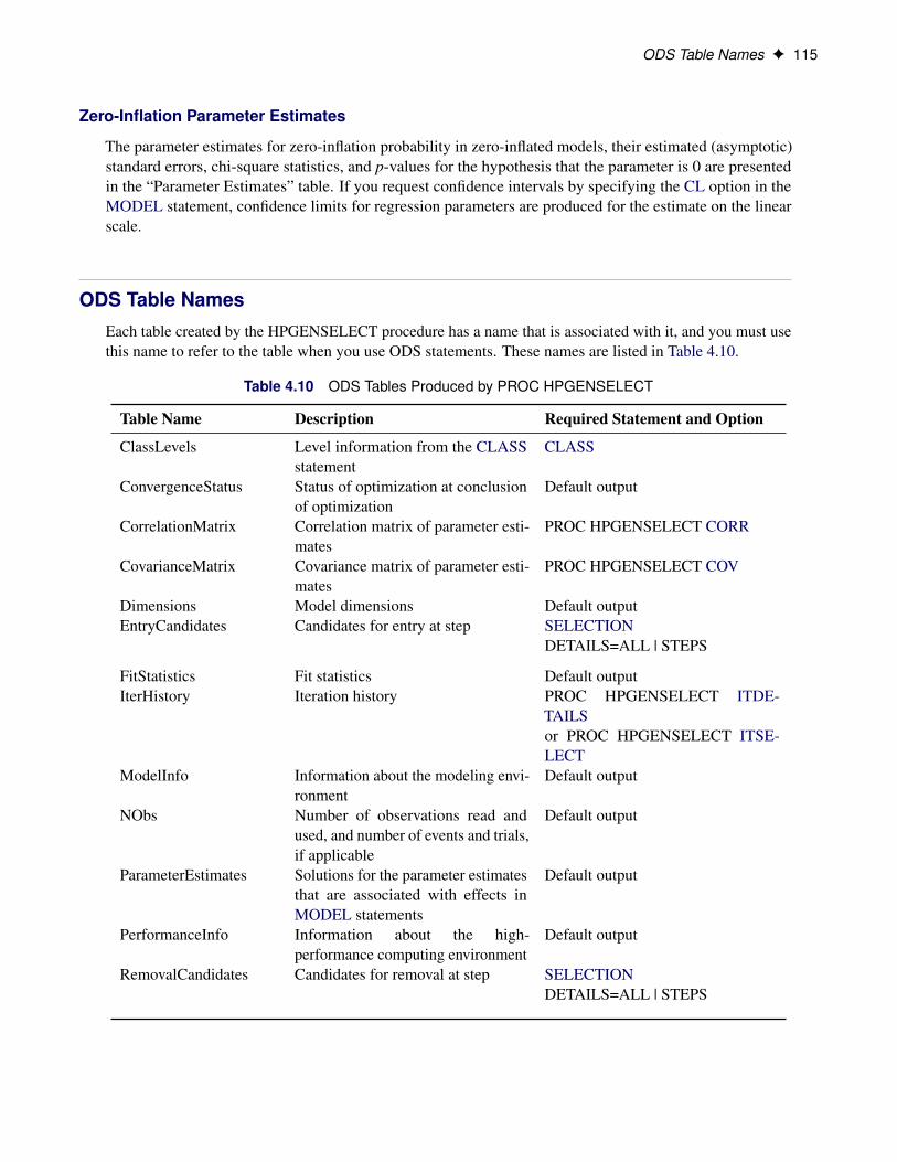
ODS Table Names F 115
Zero-Inflation Parameter Estimates
The parameter estimates for zero-inflation probability in zero-inflated models, their estimated (asymptotic)standard errors, chi-square statistics, and p-values for the hypothesis that the parameter is 0 are presentedin the “Parameter Estimates” table. If you request confidence intervals by specifying the CL option in theMODEL statement, confidence limits for regression parameters are produced for the estimate on the linearscale.
ODS Table NamesEach table created by the HPGENSELECT procedure has a name that is associated with it, and you must usethis name to refer to the table when you use ODS statements. These names are listed in Table 4.10.
Table 4.10 ODS Tables Produced by PROC HPGENSELECT
Table Name Description Required Statement and Option
ClassLevels Level information from the CLASSstatement
CLASS
ConvergenceStatus Status of optimization at conclusionof optimization
Default output
CorrelationMatrix Correlation matrix of parameter esti-mates
PROC HPGENSELECT CORR
CovarianceMatrix Covariance matrix of parameter esti-mates
PROC HPGENSELECT COV
Dimensions Model dimensions Default outputEntryCandidates Candidates for entry at step SELECTION
DETAILS=ALL | STEPS
FitStatistics Fit statistics Default outputIterHistory Iteration history PROC HPGENSELECT ITDE-
TAILSor PROC HPGENSELECT ITSE-LECT
ModelInfo Information about the modeling envi-ronment
Default output
NObs Number of observations read andused, and number of events and trials,if applicable
Default output
ParameterEstimates Solutions for the parameter estimatesthat are associated with effects inMODEL statements
Default output
PerformanceInfo Information about the high-performance computing environment
Default output
RemovalCandidates Candidates for removal at step SELECTIONDETAILS=ALL | STEPS

116 F Chapter 4: The HPGENSELECT Procedure
Table 4.10 continued
Table Name Description Required Statement / Option
ResponseProfile Response categories and the categorythat is modeled in models for binaryand multinomial data
Default output
SelectedEffects List of effects that are selected to beincluded in model
SELECTION
SelectionDetails Details about model selection, includ-ing fit statistics by step
SELECTION DETAILS=ALL
SelectionInfo Information about the settings formodel selection
SELECTION
SelectionReason Reason why the particular model wasselected
SELECTION
SelectionSummary Summary information about modelselection steps
SELECTION
StopReason Reason for termination of model se-lection
SELECTION
Timing Absolute and relative times for tasksperformed by the procedure
PERFORMANCE DETAILS
ZeroParameterEstimates Solutions for the parameter estimatesthat are associated with effects in ZE-ROMODEL statements
ZEROMODEL
Examples: HPGENSELECT Procedure
Example 4.1: Model SelectionThe following HPGENSELECT statements examine the same data that is used in the section “GettingStarted: HPGENSELECT Procedure” on page 73, but they request model selection via the forward selectiontechnique. Model effects are added in the order of their significance until no more effects make a significantimprovement of the current model. The DETAILS=ALL option in the SELECTION statement requests thatall tables that are related to model selection be produced.
The data set getStarted is shown in the section “Getting Started: HPGENSELECT Procedure” on page 73.It contains 100 observations on a count response variable (Y), a continuous variable (Total) to be used inExample 4.3, and five categorical variables (C1–C5), each of which has four numerical levels.
A log-linked Poisson regression model is specified by using classification effects for variables C1–C5. Thefollowing statements request model selection by using the forward selection method:
proc hpgenselect data=getStarted;class C1-C5;model Y = C1-C5 / Distribution=Poisson;selection method=forward details=all;
run;
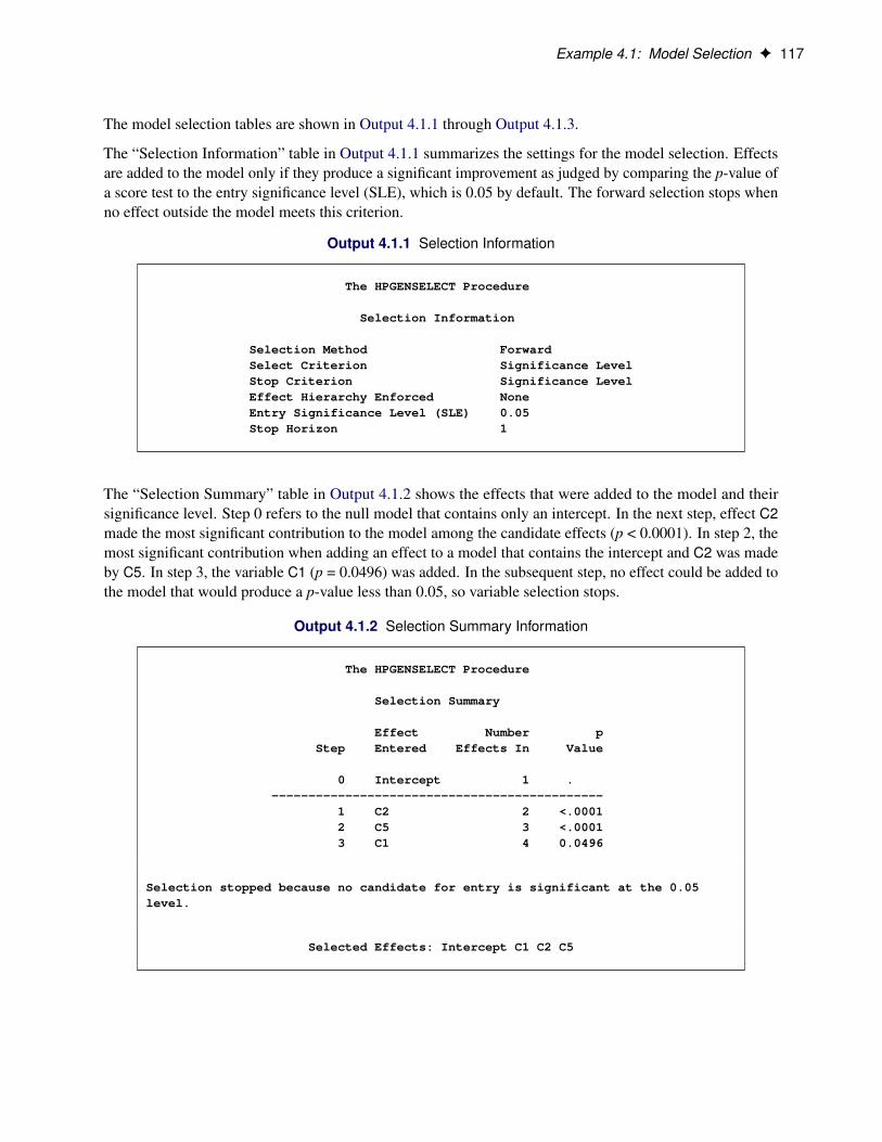
Example 4.1: Model Selection F 117
The model selection tables are shown in Output 4.1.1 through Output 4.1.3.
The “Selection Information” table in Output 4.1.1 summarizes the settings for the model selection. Effectsare added to the model only if they produce a significant improvement as judged by comparing the p-value ofa score test to the entry significance level (SLE), which is 0.05 by default. The forward selection stops whenno effect outside the model meets this criterion.
Output 4.1.1 Selection Information
The HPGENSELECT Procedure
Selection Information
Selection Method ForwardSelect Criterion Significance LevelStop Criterion Significance LevelEffect Hierarchy Enforced NoneEntry Significance Level (SLE) 0.05Stop Horizon 1
The “Selection Summary” table in Output 4.1.2 shows the effects that were added to the model and theirsignificance level. Step 0 refers to the null model that contains only an intercept. In the next step, effect C2made the most significant contribution to the model among the candidate effects (p < 0.0001). In step 2, themost significant contribution when adding an effect to a model that contains the intercept and C2 was madeby C5. In step 3, the variable C1 (p = 0.0496) was added. In the subsequent step, no effect could be added tothe model that would produce a p-value less than 0.05, so variable selection stops.
Output 4.1.2 Selection Summary Information
The HPGENSELECT Procedure
Selection Summary
Effect Number pStep Entered Effects In Value
0 Intercept 1 .---------------------------------------------
1 C2 2 <.00012 C5 3 <.00013 C1 4 0.0496
Selection stopped because no candidate for entry is significant at the 0.05level.
Selected Effects: Intercept C1 C2 C5

118 F Chapter 4: The HPGENSELECT Procedure
The DETAILS=ALL option produces the “Selection Details” table, which provides fit statistics and the valueof the score test chi-square statistic at each step.
Output 4.1.3 Selection Details
Selection Details
Effects Pr >Step Description In Model Chi-Square ChiSq -2 LogL AIC
0 Initial Model 1 350.193 352.1931 C2 entered 2 25.7340 <.0001 324.611 332.6112 C5 entered 3 23.0291 <.0001 303.580 317.5803 C1 entered 4 7.8328 0.0496 295.263 315.263
Selection Details
Step AICC BIC
0 352.234 354.7981 333.032 343.0322 318.798 335.8173 317.735 341.315
Output 4.1.4 displays information about the selected model. Notice that the –2 log likelihood value in the“Fit Statistics” table is larger than the value for the full model in Figure 4.7. This is expected because theselected model contains only a subset of the parameters. Because the selected model is more parsimoniousthan the full model, the information criteria AIC, AICC and BIC are smaller than in the full model, indicatinga better fit.
Output 4.1.4 Fit Statistics
Fit Statistics
-2 Log Likelihood 295.26316AIC (smaller is better) 315.26316AICC (smaller is better) 317.73507BIC (smaller is better) 341.31486Pearson Chi-Square 85.06563Pearson Chi-Square/DF 0.94517
The parameter estimates of the selected model are given in Output 4.1.5. Notice that the effects are listed inthe “Parameter Estimates” table in the order in which they were specified in the MODEL statement and notin the order in which they were added to the model.
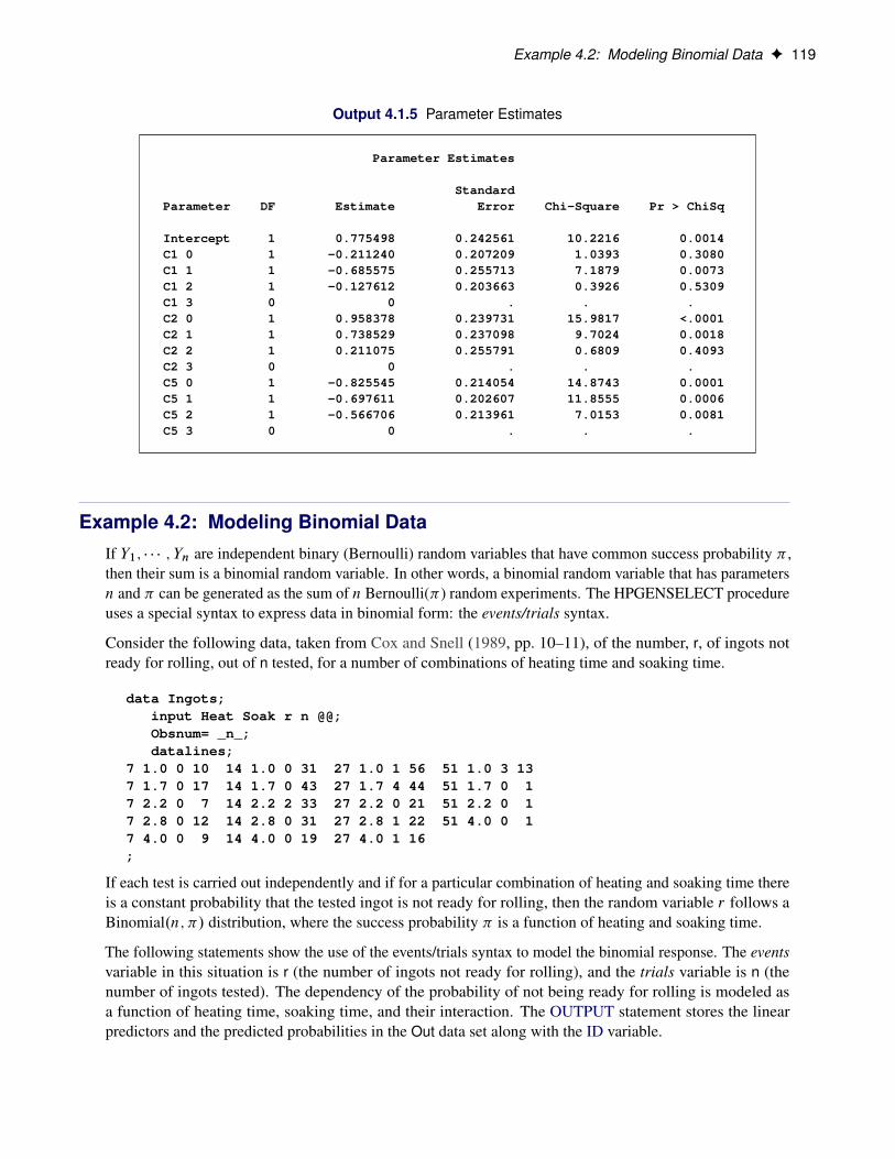
Example 4.2: Modeling Binomial Data F 119
Output 4.1.5 Parameter Estimates
Parameter Estimates
StandardParameter DF Estimate Error Chi-Square Pr > ChiSq
Intercept 1 0.775498 0.242561 10.2216 0.0014C1 0 1 -0.211240 0.207209 1.0393 0.3080C1 1 1 -0.685575 0.255713 7.1879 0.0073C1 2 1 -0.127612 0.203663 0.3926 0.5309C1 3 0 0 . . .C2 0 1 0.958378 0.239731 15.9817 <.0001C2 1 1 0.738529 0.237098 9.7024 0.0018C2 2 1 0.211075 0.255791 0.6809 0.4093C2 3 0 0 . . .C5 0 1 -0.825545 0.214054 14.8743 0.0001C5 1 1 -0.697611 0.202607 11.8555 0.0006C5 2 1 -0.566706 0.213961 7.0153 0.0081C5 3 0 0 . . .
Example 4.2: Modeling Binomial DataIf Y1; � � � ; Yn are independent binary (Bernoulli) random variables that have common success probability � ,then their sum is a binomial random variable. In other words, a binomial random variable that has parametersn and � can be generated as the sum of n Bernoulli(�) random experiments. The HPGENSELECT procedureuses a special syntax to express data in binomial form: the events/trials syntax.
Consider the following data, taken from Cox and Snell (1989, pp. 10–11), of the number, r, of ingots notready for rolling, out of n tested, for a number of combinations of heating time and soaking time.
data Ingots;input Heat Soak r n @@;Obsnum= _n_;datalines;
7 1.0 0 10 14 1.0 0 31 27 1.0 1 56 51 1.0 3 137 1.7 0 17 14 1.7 0 43 27 1.7 4 44 51 1.7 0 17 2.2 0 7 14 2.2 2 33 27 2.2 0 21 51 2.2 0 17 2.8 0 12 14 2.8 0 31 27 2.8 1 22 51 4.0 0 17 4.0 0 9 14 4.0 0 19 27 4.0 1 16;
If each test is carried out independently and if for a particular combination of heating and soaking time thereis a constant probability that the tested ingot is not ready for rolling, then the random variable r follows aBinomial.n; �/ distribution, where the success probability � is a function of heating and soaking time.
The following statements show the use of the events/trials syntax to model the binomial response. The eventsvariable in this situation is r (the number of ingots not ready for rolling), and the trials variable is n (thenumber of ingots tested). The dependency of the probability of not being ready for rolling is modeled asa function of heating time, soaking time, and their interaction. The OUTPUT statement stores the linearpredictors and the predicted probabilities in the Out data set along with the ID variable.
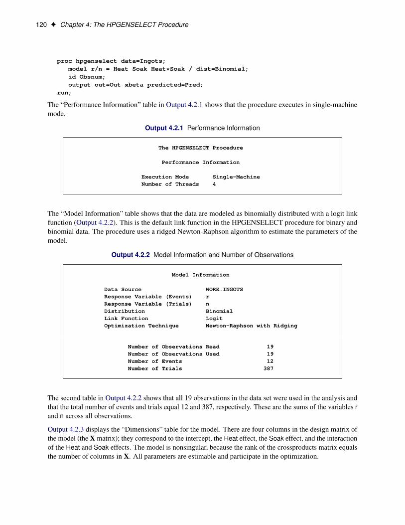
120 F Chapter 4: The HPGENSELECT Procedure
proc hpgenselect data=Ingots;model r/n = Heat Soak Heat*Soak / dist=Binomial;id Obsnum;output out=Out xbeta predicted=Pred;
run;
The “Performance Information” table in Output 4.2.1 shows that the procedure executes in single-machinemode.
Output 4.2.1 Performance Information
The HPGENSELECT Procedure
Performance Information
Execution Mode Single-MachineNumber of Threads 4
The “Model Information” table shows that the data are modeled as binomially distributed with a logit linkfunction (Output 4.2.2). This is the default link function in the HPGENSELECT procedure for binary andbinomial data. The procedure uses a ridged Newton-Raphson algorithm to estimate the parameters of themodel.
Output 4.2.2 Model Information and Number of Observations
Model Information
Data Source WORK.INGOTSResponse Variable (Events) rResponse Variable (Trials) nDistribution BinomialLink Function LogitOptimization Technique Newton-Raphson with Ridging
Number of Observations Read 19Number of Observations Used 19Number of Events 12Number of Trials 387
The second table in Output 4.2.2 shows that all 19 observations in the data set were used in the analysis andthat the total number of events and trials equal 12 and 387, respectively. These are the sums of the variables rand n across all observations.
Output 4.2.3 displays the “Dimensions” table for the model. There are four columns in the design matrix ofthe model (the X matrix); they correspond to the intercept, the Heat effect, the Soak effect, and the interactionof the Heat and Soak effects. The model is nonsingular, because the rank of the crossproducts matrix equalsthe number of columns in X. All parameters are estimable and participate in the optimization.
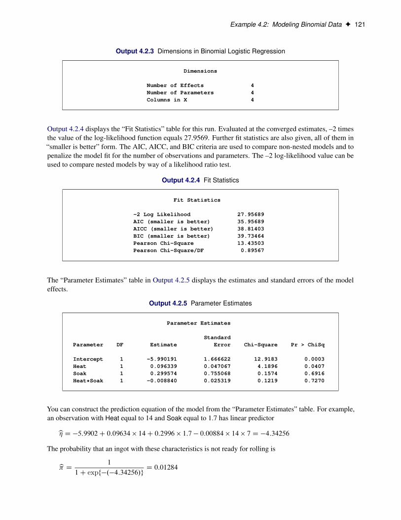
Example 4.2: Modeling Binomial Data F 121
Output 4.2.3 Dimensions in Binomial Logistic Regression
Dimensions
Number of Effects 4Number of Parameters 4Columns in X 4
Output 4.2.4 displays the “Fit Statistics” table for this run. Evaluated at the converged estimates, –2 timesthe value of the log-likelihood function equals 27.9569. Further fit statistics are also given, all of them in“smaller is better” form. The AIC, AICC, and BIC criteria are used to compare non-nested models and topenalize the model fit for the number of observations and parameters. The –2 log-likelihood value can beused to compare nested models by way of a likelihood ratio test.
Output 4.2.4 Fit Statistics
Fit Statistics
-2 Log Likelihood 27.95689AIC (smaller is better) 35.95689AICC (smaller is better) 38.81403BIC (smaller is better) 39.73464Pearson Chi-Square 13.43503Pearson Chi-Square/DF 0.89567
The “Parameter Estimates” table in Output 4.2.5 displays the estimates and standard errors of the modeleffects.
Output 4.2.5 Parameter Estimates
Parameter Estimates
StandardParameter DF Estimate Error Chi-Square Pr > ChiSq
Intercept 1 -5.990191 1.666622 12.9183 0.0003Heat 1 0.096339 0.047067 4.1896 0.0407Soak 1 0.299574 0.755068 0.1574 0.6916Heat*Soak 1 -0.008840 0.025319 0.1219 0.7270
You can construct the prediction equation of the model from the “Parameter Estimates” table. For example,an observation with Heat equal to 14 and Soak equal to 1.7 has linear predictor
b� D �5:9902C 0:09634 � 14C 0:2996 � 1:7 � 0:00884 � 14 � 7 D �4:34256The probability that an ingot with these characteristics is not ready for rolling is
b� D 1
1C expf�.�4:34256/gD 0:01284
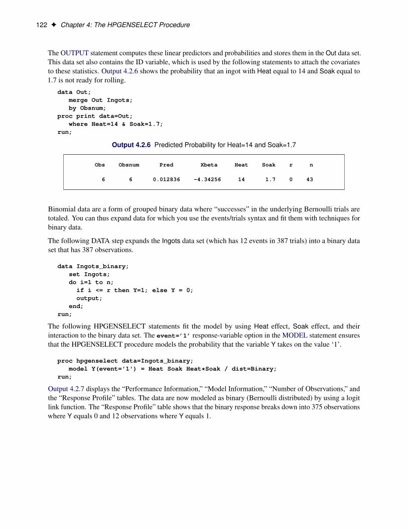
122 F Chapter 4: The HPGENSELECT Procedure
The OUTPUT statement computes these linear predictors and probabilities and stores them in the Out data set.This data set also contains the ID variable, which is used by the following statements to attach the covariatesto these statistics. Output 4.2.6 shows the probability that an ingot with Heat equal to 14 and Soak equal to1.7 is not ready for rolling.
data Out;merge Out Ingots;by Obsnum;
proc print data=Out;where Heat=14 & Soak=1.7;
run;
Output 4.2.6 Predicted Probability for Heat=14 and Soak=1.7
Obs Obsnum Pred Xbeta Heat Soak r n
6 6 0.012836 -4.34256 14 1.7 0 43
Binomial data are a form of grouped binary data where “successes” in the underlying Bernoulli trials aretotaled. You can thus expand data for which you use the events/trials syntax and fit them with techniques forbinary data.
The following DATA step expands the Ingots data set (which has 12 events in 387 trials) into a binary dataset that has 387 observations.
data Ingots_binary;set Ingots;do i=1 to n;
if i <= r then Y=1; else Y = 0;output;
end;run;
The following HPGENSELECT statements fit the model by using Heat effect, Soak effect, and theirinteraction to the binary data set. The event=’1’ response-variable option in the MODEL statement ensuresthat the HPGENSELECT procedure models the probability that the variable Y takes on the value ‘1’.
proc hpgenselect data=Ingots_binary;model Y(event='1') = Heat Soak Heat*Soak / dist=Binary;
run;
Output 4.2.7 displays the “Performance Information,” “Model Information,” “Number of Observations,” andthe “Response Profile” tables. The data are now modeled as binary (Bernoulli distributed) by using a logitlink function. The “Response Profile” table shows that the binary response breaks down into 375 observationswhere Y equals 0 and 12 observations where Y equals 1.
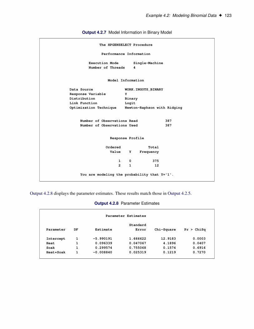
Example 4.2: Modeling Binomial Data F 123
Output 4.2.7 Model Information in Binary Model
The HPGENSELECT Procedure
Performance Information
Execution Mode Single-MachineNumber of Threads 4
Model Information
Data Source WORK.INGOTS_BINARYResponse Variable YDistribution BinaryLink Function LogitOptimization Technique Newton-Raphson with Ridging
Number of Observations Read 387Number of Observations Used 387
Response Profile
Ordered TotalValue Y Frequency
1 0 3752 1 12
You are modeling the probability that Y='1'.
Output 4.2.8 displays the parameter estimates. These results match those in Output 4.2.5.
Output 4.2.8 Parameter Estimates
Parameter Estimates
StandardParameter DF Estimate Error Chi-Square Pr > ChiSq
Intercept 1 -5.990191 1.666622 12.9183 0.0003Heat 1 0.096339 0.047067 4.1896 0.0407Soak 1 0.299574 0.755068 0.1574 0.6916Heat*Soak 1 -0.008840 0.025319 0.1219 0.7270
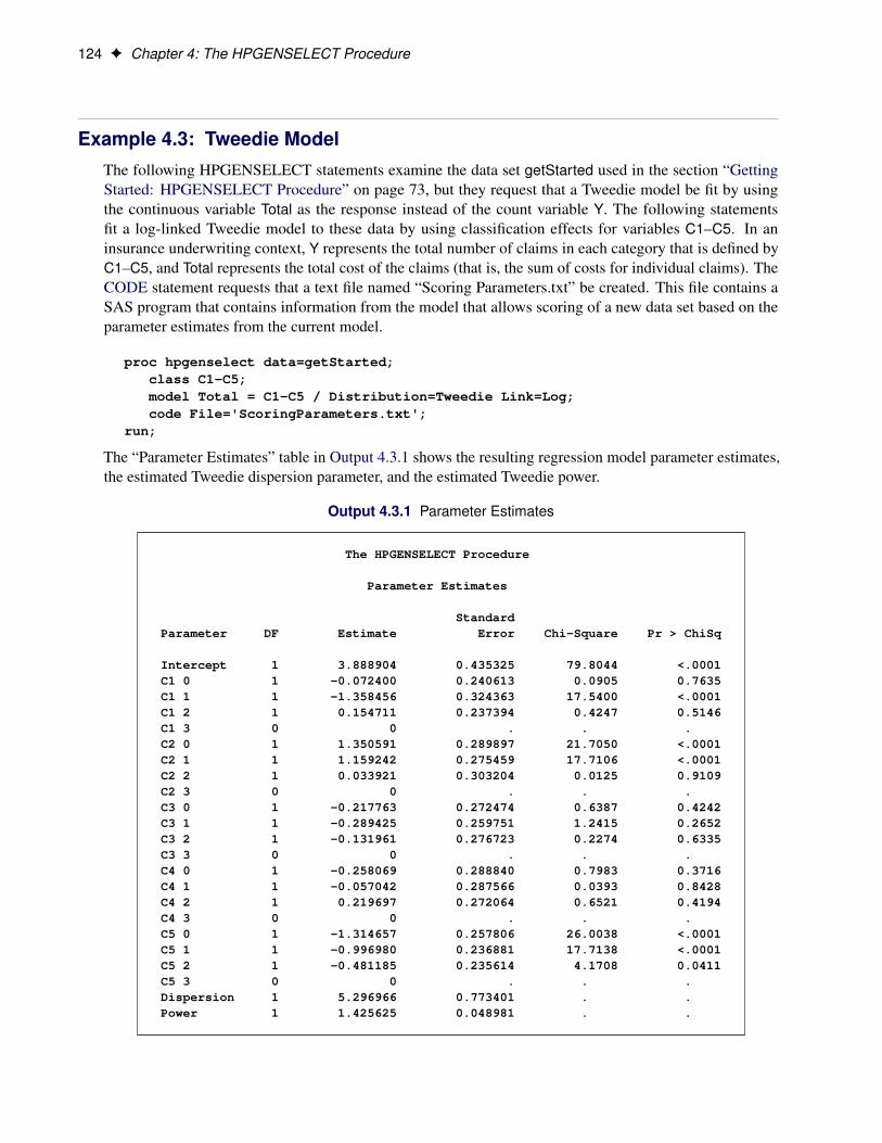
124 F Chapter 4: The HPGENSELECT Procedure
Example 4.3: Tweedie ModelThe following HPGENSELECT statements examine the data set getStarted used in the section “GettingStarted: HPGENSELECT Procedure” on page 73, but they request that a Tweedie model be fit by usingthe continuous variable Total as the response instead of the count variable Y. The following statementsfit a log-linked Tweedie model to these data by using classification effects for variables C1–C5. In aninsurance underwriting context, Y represents the total number of claims in each category that is defined byC1–C5, and Total represents the total cost of the claims (that is, the sum of costs for individual claims). TheCODE statement requests that a text file named “Scoring Parameters.txt” be created. This file contains aSAS program that contains information from the model that allows scoring of a new data set based on theparameter estimates from the current model.
proc hpgenselect data=getStarted;class C1-C5;model Total = C1-C5 / Distribution=Tweedie Link=Log;code File='ScoringParameters.txt';
run;
The “Parameter Estimates” table in Output 4.3.1 shows the resulting regression model parameter estimates,the estimated Tweedie dispersion parameter, and the estimated Tweedie power.
Output 4.3.1 Parameter Estimates
The HPGENSELECT Procedure
Parameter Estimates
StandardParameter DF Estimate Error Chi-Square Pr > ChiSq
Intercept 1 3.888904 0.435325 79.8044 <.0001C1 0 1 -0.072400 0.240613 0.0905 0.7635C1 1 1 -1.358456 0.324363 17.5400 <.0001C1 2 1 0.154711 0.237394 0.4247 0.5146C1 3 0 0 . . .C2 0 1 1.350591 0.289897 21.7050 <.0001C2 1 1 1.159242 0.275459 17.7106 <.0001C2 2 1 0.033921 0.303204 0.0125 0.9109C2 3 0 0 . . .C3 0 1 -0.217763 0.272474 0.6387 0.4242C3 1 1 -0.289425 0.259751 1.2415 0.2652C3 2 1 -0.131961 0.276723 0.2274 0.6335C3 3 0 0 . . .C4 0 1 -0.258069 0.288840 0.7983 0.3716C4 1 1 -0.057042 0.287566 0.0393 0.8428C4 2 1 0.219697 0.272064 0.6521 0.4194C4 3 0 0 . . .C5 0 1 -1.314657 0.257806 26.0038 <.0001C5 1 1 -0.996980 0.236881 17.7138 <.0001C5 2 1 -0.481185 0.235614 4.1708 0.0411C5 3 0 0 . . .Dispersion 1 5.296966 0.773401 . .Power 1 1.425625 0.048981 . .
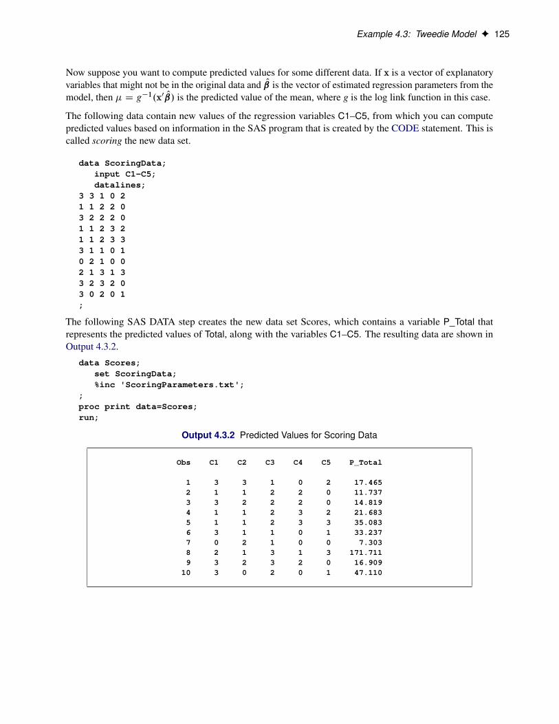
Example 4.3: Tweedie Model F 125
Now suppose you want to compute predicted values for some different data. If x is a vector of explanatoryvariables that might not be in the original data and O is the vector of estimated regression parameters from themodel, then � D g�1.x0 O/ is the predicted value of the mean, where g is the log link function in this case.
The following data contain new values of the regression variables C1–C5, from which you can computepredicted values based on information in the SAS program that is created by the CODE statement. This iscalled scoring the new data set.
data ScoringData;input C1-C5;datalines;
3 3 1 0 21 1 2 2 03 2 2 2 01 1 2 3 21 1 2 3 33 1 1 0 10 2 1 0 02 1 3 1 33 2 3 2 03 0 2 0 1;
The following SAS DATA step creates the new data set Scores, which contains a variable P_Total thatrepresents the predicted values of Total, along with the variables C1–C5. The resulting data are shown inOutput 4.3.2.
data Scores;set ScoringData;%inc 'ScoringParameters.txt';
;proc print data=Scores;run;
Output 4.3.2 Predicted Values for Scoring Data
Obs C1 C2 C3 C4 C5 P_Total
1 3 3 1 0 2 17.4652 1 1 2 2 0 11.7373 3 2 2 2 0 14.8194 1 1 2 3 2 21.6835 1 1 2 3 3 35.0836 3 1 1 0 1 33.2377 0 2 1 0 0 7.3038 2 1 3 1 3 171.7119 3 2 3 2 0 16.909
10 3 0 2 0 1 47.110
126 F Chapter 4: The HPGENSELECT Procedure
References
Akaike, H. (1974), “A New Look at the Statistical Model Identification,” IEEE Transactions on AutomaticControl, AC-19, 716–723.
Burnham, K. P. and Anderson, D. R. (1998), Model Selection and Inference: A Practical Information-Theoretic Approach, New York: Springer-Verlag.
Cox, D. R. and Snell, E. J. (1989), The Analysis of Binary Data, 2nd Edition, London: Chapman & Hall.
Dennis, J. E., Gay, D. M., and Welsch, R. E. (1981), “An Adaptive Nonlinear Least-Squares Algorithm,”ACM Transactions on Mathematical Software, 7, 348–368.
Dennis, J. E. and Mei, H. H. W. (1979), “Two New Unconstrained Optimization Algorithms Which UseFunction and Gradient Values,” Journal of Optimization Theory and Applications, 28, 453–482.
Dunn, P. K. and Smyth, G. K. (2005), “Series Evaluation of Tweedie Exponential Dispersion Model Densities,”Statistics and Computing, 15, 267–280.
Dunn, P. K. and Smyth, G. K. (2008), “Series Evaluation of Tweedie Exponential Dispersion Model Densitiesby Fourier Inversion,” Statistics and Computing, 18, 73–86.
Eskow, E. and Schnabel, R. B. (1991), “Algorithm 695: Software for a New Modified Cholesky Factorization,”ACM Transactions on Mathematical Software, 17, 306–312.
Fletcher, R. (1987), Practical Methods of Optimization, 2nd Edition, Chichester, UK: John Wiley & Sons.
Frees, E. W. (2010), Regression Modeling with Actuarial and Financial Applications, Cambridge: CambridgeUniversity Press.
Gay, D. M. (1983), “Subroutines for Unconstrained Minimization,” ACM Transactions on MathematicalSoftware, 9, 503–524.
Hurvich, C. M. and Tsai, C.-L. (1989), “Regression and Time Series Model Selection in Small Samples,”Biometrika, 76, 297–307.
Moré, J. J. and Sorensen, D. C. (1983), “Computing a Trust-Region Step,” SIAM Journal on Scientific andStatistical Computing, 4, 553–572.
Schwarz, G. (1978), “Estimating the Dimension of a Model,” Annals of Statistics, 6, 461–464.
Chapter 5
The HPLOGISTIC Procedure
ContentsOverview: HPLOGISTIC Procedure . . . . . . . . . . . . . . . . . . . . . . . . . . . . . . 128
PROC HPLOGISTIC Features . . . . . . . . . . . . . . . . . . . . . . . . . . . . . . 128PROC HPLOGISTIC Contrasted with Other SAS Procedures . . . . . . . . . . . . . 129
Getting Started: HPLOGISTIC Procedure . . . . . . . . . . . . . . . . . . . . . . . . . . . 129Binary Logistic Regression . . . . . . . . . . . . . . . . . . . . . . . . . . . . . . . 129
Syntax: HPLOGISTIC Procedure . . . . . . . . . . . . . . . . . . . . . . . . . . . . . . . 136PROC HPLOGISTIC Statement . . . . . . . . . . . . . . . . . . . . . . . . . . . . . 136BY Statement . . . . . . . . . . . . . . . . . . . . . . . . . . . . . . . . . . . . . . 141CODE Statement . . . . . . . . . . . . . . . . . . . . . . . . . . . . . . . . . . . . . 142CLASS Statement . . . . . . . . . . . . . . . . . . . . . . . . . . . . . . . . . . . . 142FREQ Statement . . . . . . . . . . . . . . . . . . . . . . . . . . . . . . . . . . . . . 143ID Statement . . . . . . . . . . . . . . . . . . . . . . . . . . . . . . . . . . . . . . . 143MODEL Statement . . . . . . . . . . . . . . . . . . . . . . . . . . . . . . . . . . . . 143OUTPUT Statement . . . . . . . . . . . . . . . . . . . . . . . . . . . . . . . . . . . 148PERFORMANCE Statement . . . . . . . . . . . . . . . . . . . . . . . . . . . . . . 150SELECTION Statement . . . . . . . . . . . . . . . . . . . . . . . . . . . . . . . . . 150WEIGHT Statement . . . . . . . . . . . . . . . . . . . . . . . . . . . . . . . . . . . 151
Details: HPLOGISTIC Procedure . . . . . . . . . . . . . . . . . . . . . . . . . . . . . . . 152Missing Values . . . . . . . . . . . . . . . . . . . . . . . . . . . . . . . . . . . . . . 152Response Distributions . . . . . . . . . . . . . . . . . . . . . . . . . . . . . . . . . . 152Log-Likelihood Functions . . . . . . . . . . . . . . . . . . . . . . . . . . . . . . . . 153Existence of Maximum Likelihood Estimates . . . . . . . . . . . . . . . . . . . . . . 154Generalized Coefficient of Determination . . . . . . . . . . . . . . . . . . . . . . . . 155The Hosmer-Lemeshow Goodness-of-Fit Test . . . . . . . . . . . . . . . . . . . . . 156Computational Method: Multithreading . . . . . . . . . . . . . . . . . . . . . . . . . 157Choosing an Optimization Algorithm . . . . . . . . . . . . . . . . . . . . . . . . . . 158
First- or Second-Order Algorithms . . . . . . . . . . . . . . . . . . . . . . . 158Algorithm Descriptions . . . . . . . . . . . . . . . . . . . . . . . . . . . . . 159
Displayed Output . . . . . . . . . . . . . . . . . . . . . . . . . . . . . . . . . . . . . 161ODS Table Names . . . . . . . . . . . . . . . . . . . . . . . . . . . . . . . . . . . . 165
Examples: HPLOGISTIC Procedure . . . . . . . . . . . . . . . . . . . . . . . . . . . . . . 166Example 5.1: Model Selection . . . . . . . . . . . . . . . . . . . . . . . . . . . . . 166Example 5.2: Modeling Binomial Data . . . . . . . . . . . . . . . . . . . . . . . . . 170Example 5.3: Ordinal Logistic Regression . . . . . . . . . . . . . . . . . . . . . . . 175Example 5.4: Conditional Logistic Regression for Matched Pairs Data . . . . . . . . 178
References . . . . . . . . . . . . . . . . . . . . . . . . . . . . . . . . . . . . . . . . . . . 182

128 F Chapter 5: The HPLOGISTIC Procedure
Overview: HPLOGISTIC ProcedureThe HPLOGISTIC procedure is a high-performance procedure that fits logistic regression models for binary,binomial, and multinomial data on the SAS appliance.
The HPLOGISTIC procedure fits logistic regression models in the broader sense; the procedure permitsseveral link functions and can handle ordinal and nominal data with more than two response categories(multinomial data).
PROC HPLOGISTIC runs in either single-machine mode or distributed mode.
NOTE: Distributed mode requires SAS High-Performance Statistics.
PROC HPLOGISTIC FeaturesThe HPLOGISTIC procedure estimates the parameters of a logistic regression model by using maximumlikelihood techniques. It also does the following:
• provides model-building syntax with the CLASS and effect-based MODEL statements, which arefamiliar from SAS/STAT analytic procedures (in particular, the GLM, LOGISTIC, GLIMMIX, andMIXED procedures)
• provides response-variable options as in the LOGISTIC procedure
• performs maximum likelihood estimation
• provides multiple link functions
• provides cumulative link models for ordinal data and generalized logit modeling for unordered multi-nomial data
• enables model building (variable selection) through the SELECTION statement
• provides a WEIGHT statement for weighted analysis
• provides a FREQ statement for grouped analysis
• provides an OUTPUT statement to produce a data set with predicted probabilities and other observa-tionwise statistics
Because the HPLOGISTIC procedure is a high-performance analytical procedure, it also does the following:
• enables you to run in distributed mode on a cluster of machines that distribute the data and thecomputations
• enables you to run in single-machine mode on the server where SAS is installed
• exploits all the available cores and concurrent threads, regardless of execution mode
PROC HPLOGISTIC Contrasted with Other SAS Procedures F 129
• performs parallel reads of input data and parallel writes of output data when the data source is theappliance database
For more information, see the section “Processing Modes” on page 6 in Chapter 2, “Shared Concepts andTopics.”
PROC HPLOGISTIC Contrasted with Other SAS ProceduresFor general contrasts, see the section “Common Features of SAS High-Performance Statistical Procedures”on page 40. The following remarks contrast the HPLOGISTIC procedure with the LOGISTIC procedure inSAS/STAT software.
The CLASS statement in the HPLOGISTIC procedure permits two parameterizations: the GLM parameteri-zation and a reference parameterization. In contrast to the LOGISTIC, GENMOD, and other procedures thatpermit multiple parameterizations, the HPLOGISTIC procedure does not mix parameterizations across thevariables in the CLASS statement. In other words, all classification variables have the same parameterization,and this parameterization is either the GLM or reference parameterization.
The default parameterization of CLASS variables in the HPLOGISTIC procedure is the GLM parameteriza-tion. The LOGISTIC procedure uses the EFFECT parameterization for the CLASS variables by default. Ineither procedure, you can change the parameterization with the PARAM= option in the CLASS statement.
The default optimization technique used by the LOGISTIC procedure is Fisher scoring; the HPLOGISTICprocedure uses by default a modification of the Newton-Raphson algorithm with a ridged Hessian. You canchoose different optimization techniques, including first-order methods that do not require a crossproductsmatrix or Hessian, with the TECHNIQUE= option in the PROC HPLOGISTIC statement.
The LOGISTIC procedure offers a wide variety of postfitting analyses, such as contrasts, estimates, tests ofmodel effects, least squares means, and odds ratios. This release of the HPLOGISTIC procedure is limited inpostfitting functionality, since with large data sets the focus is primarily on model fitting and scoring.
The HPLOGISTIC procedure is specifically designed to operate in the high-performance distributed envi-ronment. By default, PROC HPLOGISTIC performs computations in multiple threads. The LOGISTICprocedure executes in a single thread.
Getting Started: HPLOGISTIC Procedure
Binary Logistic RegressionThe following DATA step contains 100 observations on a dichotomous response variable (y), a charactervariable (C), and 10 continuous variables (x1–x10):
data getStarted;input C$ y x1-x10;datalines;D 0 10.2 6 1.6 38 15 2.4 20 0.8 8.5 3.9
130 F Chapter 5: The HPLOGISTIC Procedure
F 1 12.2 6 2.6 42 61 1.5 10 0.6 8.5 0.7D 1 7.7 1 2.1 38 61 1 90 0.6 7.5 5.2J 1 10.9 7 3.5 46 42 0.3 0 0.2 6 3.6E 0 17.3 6 3.8 26 47 0.9 10 0.4 1.5 4.7A 0 18.7 4 1.8 2 34 1.7 80 1 9.5 2.2B 0 7.2 1 0.3 48 61 1.1 10 0.8 3.5 4D 0 0.1 3 2.4 0 65 1.6 70 0.8 3.5 0.7H 1 2.4 4 0.7 38 22 0.2 20 0 3 4.2J 0 15.6 7 1.4 0 98 0.3 0 1 5 5.2J 0 11.1 3 2.4 42 55 2.2 60 0.6 4.5 0.7F 0 4 6 0.9 4 36 2.1 30 0.8 9 4.6A 0 6.2 2 1.8 14 79 1.1 70 0.2 0 5.1H 0 3.7 3 0.8 12 66 1.3 40 0.4 0.5 3.3A 1 9.2 3 2.3 48 51 2.3 50 0 6 5.4G 0 14 3 2 18 12 2.2 0 0 3 3.4E 1 19.5 6 3.7 26 81 0.1 30 0.6 5 4.8C 0 11 3 2.8 38 9 1.7 50 0.8 6.5 0.9I 0 15.3 7 2.2 20 98 2.7 100 0.4 7 0.8H 1 7.4 4 0.5 28 65 1.3 60 0.2 9.5 5.4F 0 11.4 2 1.4 42 12 2.4 10 0.4 1 4.5C 1 19.4 1 0.4 42 4 2.4 10 0 6.5 0.1G 0 5.9 4 2.6 12 57 0.8 50 0.4 2 5.8G 1 15.8 6 3.7 34 8 1.3 90 0.6 2.5 5.7I 0 10 3 1.9 16 80 3 90 0.4 9.5 1.9E 0 15.7 1 2.7 32 25 1.7 20 0.2 8.5 6G 0 11 5 2.9 48 53 0.1 50 1 3.5 1.2J 1 16.8 0 0.9 14 86 1.4 40 0.8 9 5D 1 11 4 3.2 48 63 2.8 90 0.6 0 2.2J 1 4.8 7 3.6 24 1 2.2 20 1 8.5 0.5J 1 10.4 5 2 42 56 1 20 0 3.5 4.2G 0 12.7 7 3.6 8 56 2.1 70 1 4.5 1.5G 0 6.8 1 3.2 30 27 0.6 0 0.8 2 5.6E 0 8.8 0 3.2 2 67 0.7 10 0.4 1 5I 1 0.2 0 2.9 10 41 2.3 60 0.2 9 0.3J 1 4.6 7 3.9 50 61 2.1 50 0.4 3 4.9J 1 2.3 2 3.2 36 98 0.1 40 0.6 4.5 4.3I 0 10.8 3 2.7 28 58 0.8 80 0.8 3 6B 0 9.3 2 3.3 44 44 0.3 50 0.8 5.5 0.4F 0 9.2 6 0.6 4 64 0.1 0 0.6 4.5 3.9D 0 7.4 0 2.9 14 0 0.2 30 0.8 7.5 4.5G 0 18.3 3 3.1 8 60 0.3 60 0.2 7 1.9F 0 5.3 4 0.2 48 63 2.3 80 0.2 8 5.2C 0 2.6 5 2.2 24 4 1.3 20 0 2 1.4F 0 13.8 4 3.6 4 7 1.1 10 0.4 3.5 1.9B 1 12.4 6 1.7 30 44 1.1 60 0.2 6 1.5I 0 1.3 1 1.3 8 53 1.1 70 0.6 7 0.8F 0 18.2 7 1.7 26 92 2.2 30 1 8.5 4.8J 0 5.2 2 2.2 18 12 1.4 90 0.8 4 4.9G 1 9.4 2 0.8 22 86 0.4 30 0.4 1 5.9J 1 10.4 2 1.7 26 31 2.4 10 0.2 7 1.6J 0 13 1 1.8 14 11 2.3 50 0.6 5.5 2.6A 0 17.9 4 3.1 46 58 2.6 90 0.6 1.5 3.2D 1 19.4 6 3 20 50 2.8 100 0.2 9 1.2I 0 19.6 3 3.6 22 19 1.2 0 0.6 5 4.1
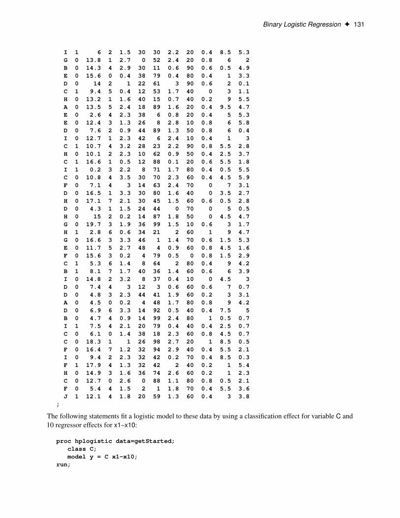
Binary Logistic Regression F 131
I 1 6 2 1.5 30 30 2.2 20 0.4 8.5 5.3G 0 13.8 1 2.7 0 52 2.4 20 0.8 6 2B 0 14.3 4 2.9 30 11 0.6 90 0.6 0.5 4.9E 0 15.6 0 0.4 38 79 0.4 80 0.4 1 3.3D 0 14 2 1 22 61 3 90 0.6 2 0.1C 1 9.4 5 0.4 12 53 1.7 40 0 3 1.1H 0 13.2 1 1.6 40 15 0.7 40 0.2 9 5.5A 0 13.5 5 2.4 18 89 1.6 20 0.4 9.5 4.7E 0 2.6 4 2.3 38 6 0.8 20 0.4 5 5.3E 0 12.4 3 1.3 26 8 2.8 10 0.8 6 5.8D 0 7.6 2 0.9 44 89 1.3 50 0.8 6 0.4I 0 12.7 1 2.3 42 6 2.4 10 0.4 1 3C 1 10.7 4 3.2 28 23 2.2 90 0.8 5.5 2.8H 0 10.1 2 2.3 10 62 0.9 50 0.4 2.5 3.7C 1 16.6 1 0.5 12 88 0.1 20 0.6 5.5 1.8I 1 0.2 3 2.2 8 71 1.7 80 0.4 0.5 5.5C 0 10.8 4 3.5 30 70 2.3 60 0.4 4.5 5.9F 0 7.1 4 3 14 63 2.4 70 0 7 3.1D 0 16.5 1 3.3 30 80 1.6 40 0 3.5 2.7H 0 17.1 7 2.1 30 45 1.5 60 0.6 0.5 2.8D 0 4.3 1 1.5 24 44 0 70 0 5 0.5H 0 15 2 0.2 14 87 1.8 50 0 4.5 4.7G 0 19.7 3 1.9 36 99 1.5 10 0.6 3 1.7H 1 2.8 6 0.6 34 21 2 60 1 9 4.7G 0 16.6 3 3.3 46 1 1.4 70 0.6 1.5 5.3E 0 11.7 5 2.7 48 4 0.9 60 0.8 4.5 1.6F 0 15.6 3 0.2 4 79 0.5 0 0.8 1.5 2.9C 1 5.3 6 1.4 8 64 2 80 0.4 9 4.2B 1 8.1 7 1.7 40 36 1.4 60 0.6 6 3.9I 0 14.8 2 3.2 8 37 0.4 10 0 4.5 3D 0 7.4 4 3 12 3 0.6 60 0.6 7 0.7D 0 4.8 3 2.3 44 41 1.9 60 0.2 3 3.1A 0 4.5 0 0.2 4 48 1.7 80 0.8 9 4.2D 0 6.9 6 3.3 14 92 0.5 40 0.4 7.5 5B 0 4.7 4 0.9 14 99 2.4 80 1 0.5 0.7I 1 7.5 4 2.1 20 79 0.4 40 0.4 2.5 0.7C 0 6.1 0 1.4 38 18 2.3 60 0.8 4.5 0.7C 0 18.3 1 1 26 98 2.7 20 1 8.5 0.5F 0 16.4 7 1.2 32 94 2.9 40 0.4 5.5 2.1I 0 9.4 2 2.3 32 42 0.2 70 0.4 8.5 0.3F 1 17.9 4 1.3 32 42 2 40 0.2 1 5.4H 0 14.9 3 1.6 36 74 2.6 60 0.2 1 2.3C 0 12.7 0 2.6 0 88 1.1 80 0.8 0.5 2.1F 0 5.4 4 1.5 2 1 1.8 70 0.4 5.5 3.6J 1 12.1 4 1.8 20 59 1.3 60 0.4 3 3.8
;
The following statements fit a logistic model to these data by using a classification effect for variable C and10 regressor effects for x1–x10:
proc hplogistic data=getStarted;class C;model y = C x1-x10;
run;

132 F Chapter 5: The HPLOGISTIC Procedure
The default output from this analysis is presented in Figure 5.1 through Figure 5.11.
The “Performance Information” table in Figure 5.1 shows that the procedure executes in single-machinemode—that is, the model is fit on the machine where the SAS session executes. This run of the HPLOGISTICprocedure was performed on a multicore machine with the same number of CPUs as there are threads; that is,one computational thread was spawned per CPU.
Figure 5.1 Performance Information
The HPLOGISTIC Procedure
Performance Information
Execution Mode Single-MachineNumber of Threads 4
Figure 5.2 displays the “Model Information” table. The HPLOGISTIC procedure uses a Newton-Raphsonalgorithm to model a binary distribution for the variable y with a logit link function. The CLASS variable Cis parameterized using the GLM parameterization, which is the default.
Figure 5.2 Model Information
Model Information
Data Source WORK.GETSTARTEDResponse Variable yClass Parameterization GLMDistribution BinaryLink Function LogitOptimization Technique Newton-Raphson with Ridging
The CLASS variable C has 10 unique formatted levels, and these are displayed in the “Class Level Information”table in Figure 5.3.
Figure 5.3 Class Level Information
Class Level Information
Class Levels Values
C 10 A B C D E F G H I J
Figure 5.4 displays the “Number of Observations” table. All 100 observations in the data set are used in theanalysis.
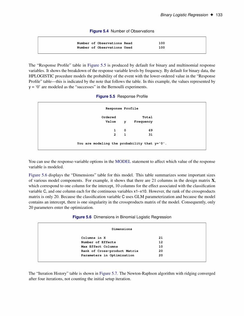
Binary Logistic Regression F 133
Figure 5.4 Number of Observations
Number of Observations Read 100Number of Observations Used 100
The “Response Profile” table in Figure 5.5 is produced by default for binary and multinomial responsevariables. It shows the breakdown of the response variable levels by frequency. By default for binary data, theHPLOGISTIC procedure models the probability of the event with the lower-ordered value in the “ResponseProfile” table—this is indicated by the note that follows the table. In this example, the values represented byy = ‘0’ are modeled as the “successes” in the Bernoulli experiments.
Figure 5.5 Response Profile
Response Profile
Ordered TotalValue y Frequency
1 0 692 1 31
You are modeling the probability that y='0'.
You can use the response-variable options in the MODEL statement to affect which value of the responsevariable is modeled.
Figure 5.6 displays the “Dimensions” table for this model. This table summarizes some important sizesof various model components. For example, it shows that there are 21 columns in the design matrix X,which correspond to one column for the intercept, 10 columns for the effect associated with the classificationvariable C, and one column each for the continuous variables x1–x10. However, the rank of the crossproductsmatrix is only 20. Because the classification variable C uses GLM parameterization and because the modelcontains an intercept, there is one singularity in the crossproducts matrix of the model. Consequently, only20 parameters enter the optimization.
Figure 5.6 Dimensions in Binomial Logistic Regression
Dimensions
Columns in X 21Number of Effects 12Max Effect Columns 10Rank of Cross-product Matrix 20Parameters in Optimization 20
The “Iteration History” table is shown in Figure 5.7. The Newton-Raphson algorithm with ridging convergedafter four iterations, not counting the initial setup iteration.
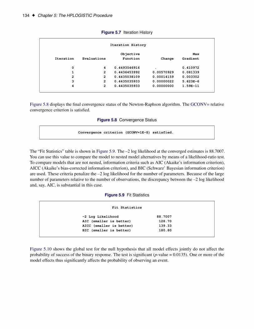
134 F Chapter 5: The HPLOGISTIC Procedure
Figure 5.7 Iteration History
Iteration History
Objective MaxIteration Evaluations Function Change Gradient
0 4 0.4493546916 . 0.4109721 2 0.4436453992 0.00570929 0.0813392 2 0.4435038109 0.00014159 0.0033023 2 0.4435035933 0.00000022 5.623E-64 2 0.4435035933 0.00000000 1.59E-11
Figure 5.8 displays the final convergence status of the Newton-Raphson algorithm. The GCONV= relativeconvergence criterion is satisfied.
Figure 5.8 Convergence Status
Convergence criterion (GCONV=1E-8) satisfied.
The “Fit Statistics” table is shown in Figure 5.9. The –2 log likelihood at the converged estimates is 88.7007.You can use this value to compare the model to nested model alternatives by means of a likelihood-ratio test.To compare models that are not nested, information criteria such as AIC (Akaike’s information criterion),AICC (Akaike’s bias-corrected information criterion), and BIC (Schwarz’ Bayesian information criterion)are used. These criteria penalize the –2 log likelihood for the number of parameters. Because of the largenumber of parameters relative to the number of observations, the discrepancy between the –2 log likelihoodand, say, AIC, is substantial in this case.
Figure 5.9 Fit Statistics
Fit Statistics
-2 Log Likelihood 88.7007AIC (smaller is better) 128.70AICC (smaller is better) 139.33BIC (smaller is better) 180.80
Figure 5.10 shows the global test for the null hypothesis that all model effects jointly do not affect theprobability of success of the binary response. The test is significant (p-value = 0.0135). One or more of themodel effects thus significantly affects the probability of observing an event.
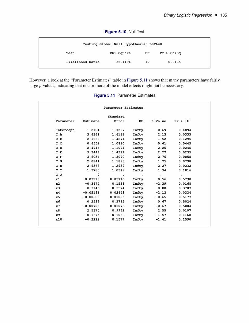
Binary Logistic Regression F 135
Figure 5.10 Null Test
Testing Global Null Hypothesis: BETA=0
Test Chi-Square DF Pr > ChiSq
Likelihood Ratio 35.1194 19 0.0135
However, a look at the “Parameter Estimates” table in Figure 5.11 shows that many parameters have fairlylarge p-values, indicating that one or more of the model effects might not be necessary.
Figure 5.11 Parameter Estimates
Parameter Estimates
StandardParameter Estimate Error DF t Value Pr > |t|
Intercept 1.2101 1.7507 Infty 0.69 0.4894C A 3.4341 1.6131 Infty 2.13 0.0333C B 2.1638 1.4271 Infty 1.52 0.1295C C 0.6552 1.0810 Infty 0.61 0.5445C D 2.4945 1.1094 Infty 2.25 0.0245C E 3.2449 1.4321 Infty 2.27 0.0235C F 3.6054 1.3070 Infty 2.76 0.0058C G 2.0841 1.1898 Infty 1.75 0.0798C H 2.9368 1.2939 Infty 2.27 0.0232C I 1.3785 1.0319 Infty 1.34 0.1816C J 0 . . . .x1 0.03218 0.05710 Infty 0.56 0.5730x2 -0.3677 0.1538 Infty -2.39 0.0168x3 0.3146 0.3574 Infty 0.88 0.3787x4 -0.05196 0.02443 Infty -2.13 0.0334x5 -0.00683 0.01056 Infty -0.65 0.5177x6 0.2539 0.3785 Infty 0.67 0.5024x7 -0.00723 0.01073 Infty -0.67 0.5004x8 2.5370 0.9942 Infty 2.55 0.0107x9 -0.1675 0.1068 Infty -1.57 0.1168x10 -0.2222 0.1577 Infty -1.41 0.1590

136 F Chapter 5: The HPLOGISTIC Procedure
Syntax: HPLOGISTIC ProcedureThe following statements are available in the HPLOGISTIC procedure:
PROC HPLOGISTIC < options > ;BY variables ;CLASS variable < (options) >: : : < variable < (options) > > < / global-options > ;CODE < options > ;FREQ variable ;ID variables ;MODEL response< (response-options) > = < effects > < / model-options > ;MODEL events/trials< (response-options) > = < effects > < / model-options > ;OUTPUT < OUT=SAS-data-set >
< keyword < =name > >. . .< keyword < =name > > < / options > ;
PERFORMANCE performance-options ;SELECTION selection-options ;WEIGHT variable ;
The PROC HPLOGISTIC statement and at least one MODEL statement is required. The CLASS statementcan appear multiple times. If a CLASS statement is specified, it must precede the MODEL statements.
PROC HPLOGISTIC StatementPROC HPLOGISTIC < options > ;
The PROC HPLOGISTIC statement invokes the procedure. Table 5.1 summarizes the available options inthe PROC HPLOGISTIC statement by function. The options are then described fully in alphabetical order.
Table 5.1 PROC HPLOGISTIC Statement Options
Option Description
Basic OptionsALPHA= Specifies a global significance levelDATA= Specifies the input data setNAMELEN= Limits the length of effect names
Options Related to OutputITDETAILS Adds detail information to “Iteration History” tableITSELECT Displays the “Iteration History” table with model selectionNOPRINT Suppresses ODS outputNOCLPRINT Limits or suppresses the display of class levelsNOITPRINT Suppresses generation of the iteration history tableNOSTDERR Suppresses computation of covariance matrix and standard errors
PROC HPLOGISTIC Statement F 137
Table 5.1 continued
Option Description
Options Related to OptimizationABSCONV= Tunes the absolute function convergence criterionABSFCONV= Tunes the absolute function difference convergence criterionABSGCONV= Tunes the absolute gradient convergence criterionFCONV= Tunes the relative function difference convergence criterionGCONV= Tunes the relative gradient convergence criterionMAXITER= Chooses the maximum number of iterations in any optimizationMAXFUNC= Specifies the maximum number of function evaluations in any optimizationMAXTIME= Specifies the upper limit of CPU time (in seconds) for any optimizationMINITER= Specifies the minimum number of iterations in any optimizationNORMALIZE= Specifies whether the objective function is normalized during optimizationTECHNIQUE= Selects the optimization technique
TolerancesSINGCHOL= Tunes the singularity criterion for Cholesky decompositionsSINGSWEEP= Tunes the singularity criterion for the sweep operatorSINGULAR= Tunes the general singularity criterion
User-Defined FormatsFMTLIBXML= Specifies the file reference for a format stream
You can specify the following options in the PROC HPLOGISTIC statement.
ABSCONV=r
ABSTOL=rspecifies an absolute function convergence criterion. For minimization, termination requires f . .k// �r, where is the vector of parameters in the optimization and f .�/ is the objective function. Thedefault value of r is the negative square root of the largest double-precision value, which serves only asa protection against overflows.
ABSFCONV=r < n >
ABSFTOL=r < n >specifies an absolute function difference convergence criterion. For all techniques except NMSIMP,termination requires a small change of the function value in successive iterations:
jf . .k�1// � f . .k//j � r
Here, denotes the vector of parameters that participate in the optimization, and f .�/ is the objectivefunction. The same formula is used for the NMSIMP technique, but .k/ is defined as the vertex withthe lowest function value and .k�1/ is defined as the vertex with the highest function value in thesimplex. The default value is r = 0. The optional integer value n specifies the number of successiveiterations for which the criterion must be satisfied before the process can be terminated.
138 F Chapter 5: The HPLOGISTIC Procedure
ABSGCONV=r < n >
ABSGTOL=r < n >specifies an absolute gradient convergence criterion. Termination requires the maximum absolutegradient element to be small:
maxjjgj .
.k//j � r
Here, denotes the vector of parameters that participate in the optimization, and gj .�/ is the gradientof the objective function with respect to the j th parameter. This criterion is not used by the NMSIMPtechnique. The default value is r=1E–5. The optional integer value n specifies the number of successiveiterations for which the criterion must be satisfied before the process can be terminated.
ALPHA=numberspecifies a global significance level for the construction of confidence intervals. The confidence levelis 1–number. The value of number must be between 0 and 1; the default is 0.05. You can override theglobal specification with the ALPHA= option in the MODEL statement.
DATA=SAS-data-setnames the input SAS data set for PROC HPLOGISTIC to use. The default is the most recently createddata set.
If the procedure executes in distributed mode, the input data are distributed to memory on the appliancenodes and analyzed in parallel, unless the data are already distributed in the appliance database. Inthat case the procedure reads the data alongside the distributed database. For information about thevarious execution modes, see the section “Processing Modes” on page 6; for information about thealongside-the-database model, see the section “Alongside-the-Database Execution” on page 13.
FCONV=r < n >
FTOL=r < n >specifies a relative function difference convergence criterion. For all techniques except NMSIMP,termination requires a small relative change of the function value in successive iterations,
jf . .k// � f . .k�1//j
jf . .k�1//j� r
Here, denotes the vector of parameters that participate in the optimization, and f .�/ is the objectivefunction. The same formula is used for the NMSIMP technique, but .k/ is defined as the vertex withthe lowest function value, and .k�1/ is defined as the vertex with the highest function value in thesimplex.
The default value is r=2 � � where � is the machine precision. The optional integer value n specifiesthe number of successive iterations for which the criterion must be satisfied before the process canterminate.
FMTLIBXML=file-refspecifies the file reference for the XML stream that contains the user-defined format definitions. User-defined formats are handled differently in a distributed computing environment than they are in otherSAS products. See the section “Working with Formats” on page 32 for details about how to generate aXML stream for your formats.
PROC HPLOGISTIC Statement F 139
GCONV=r < n >
GTOL=r < n >specifies a relative gradient convergence criterion. For all techniques except CONGRA and NMSIMP,termination requires that the normalized predicted function reduction be small,
g. .k//0ŒH.k/��1g. .k//jf . .k//j
� r
Here, denotes the vector of parameters that participate in the optimization, f .�/ is the objectivefunction, and g.�/ is the gradient. For the CONGRA technique (where a reliable Hessian estimate H isnot available), the following criterion is used:
k g. .k// k22 k s. .k// k2k g. .k// � g. .k�1// k2 jf . .k//j
� r
This criterion is not used by the NMSIMP technique. The default value is r=1E–8. The optional integervalue n specifies the number of successive iterations for which the criterion must be satisfied beforethe process can terminate.
ITDETAILSadds to the “Iteration History” table the current values of the parameter estimates and their gradients.These quantities are reported only for parameters that participate in the optimization. The ITDETAILSoption is not available with model selection.
ITSELECTgenerates the “Iteration History” table when you perform a model selection.
MAXFUNC=n
MAXFU=nspecifies the maximum number n of function calls in the optimization process. The default values areas follows, depending on the optimization technique:
• TRUREG, NRRIDG, NEWRAP: 125
• QUANEW, DBLDOG: 500
• CONGRA: 1,000
• NMSIMP: 3,000
The optimization can terminate only after completing a full iteration. Therefore, the number of functioncalls that are actually performed can exceed the number that is specified by the MAXFUNC= option.You can choose the optimization technique with the TECHNIQUE= option.
MAXITER=n
MAXIT=nspecifies the maximum number n of iterations in the optimization process. The default values are asfollows, depending on the optimization technique:
• TRUREG, NRRIDG, NEWRAP: 50
140 F Chapter 5: The HPLOGISTIC Procedure
• QUANEW, DBLDOG: 200
• CONGRA: 400
• NMSIMP: 1,000
These default values also apply when n is specified as a missing value. You can choose the optimizationtechnique with the TECHNIQUE= option.
MAXTIME=rspecifies an upper limit of r seconds of CPU time for the optimization process. The default value is thelargest floating-point double representation of your computer. The time specified by the MAXTIME=option is checked only once at the end of each iteration. Therefore, the actual running time can belonger than that specified by the MAXTIME= option.
MINITER=n
MINIT=nspecifies the minimum number of iterations. The default value is 0. If you request more iterationsthan are actually needed for convergence to a stationary point, the optimization algorithms can behavestrangely. For example, the effect of rounding errors can prevent the algorithm from continuing for therequired number of iterations.
NAMELEN=numberspecifies the length to which long effect names are shortened. The default and minimum value is 20.
NOCLPRINT< =number >suppresses the display of the “Class Level Information” table if you do not specify number. If youspecify number, the values of the classification variables are displayed for only those variables whosenumber of levels is less than number. Specifying a number helps to reduce the size of the “Class LevelInformation” table if some classification variables have a large number of levels.
NOITPRINTsuppresses the generation of the “Iteration History” table.
NOPRINTsuppresses the generation of ODS output.
NORMALIZE=YES | NOspecifies whether the objective function should be normalized during the optimization by the reciprocalof the used frequency count. The default is to normalize the objective function. This option affects thevalues reported in the “Iteration History” table. The results reported in the “Fit Statistics” are alwaysdisplayed for the nonnormalized log-likelihood function.
NOSTDERRsuppresses the computation of the covariance matrix and the standard errors of the logistic regressioncoefficients. When the model contains many variables (thousands), the inversion of the Hessianmatrix to derive the covariance matrix and the standard errors of the regression coefficients can betime-consuming.
BY Statement F 141
SINGCHOL=numbertunes the singularity criterion in Cholesky decompositions. The default is 1E7 times the machineepsilon; this product is approximately 1E–9 on most computers.
SINGSWEEP=numbertunes the singularity criterion for sweep operations. The default is 1E7 times the machine epsilon; thisproduct is approximately 1E–9 on most computers.
SINGULAR=numbertunes the general singularity criterion applied by the HPLOGISTIC procedure in sweeps and inversions.The default is 1E7 times the machine epsilon; this product is approximately 1E–9 on most computers.
TECHNIQUE=keyword
TECH=keywordspecifies the optimization technique for obtaining maximum likelihood estimates. You can choosefrom the following techniques by specifying the appropriate keyword :
CONGRA performs a conjugate-gradient optimization.
DBLDOG performs a version of double-dogleg optimization.
NEWRAP performs a Newton-Raphson optimization with line search.
NMSIMP performs a Nelder-Mead simplex optimization.
NONE performs no optimization.
NRRIDG performs a Newton-Raphson optimization with ridging.
QUANEW performs a dual quasi-Newton optimization.
TRUREG performs a trust-region optimization
The default value is TECHNIQUE=NRRIDG.
For more information, see the section “Choosing an Optimization Algorithm” on page 158.
BY StatementBY variables ;
You can specify a BY statement in PROC HPLOGISTIC to obtain separate analyses of observations in groupsthat are defined by the BY variables. When a BY statement appears, PROC HPLOGISTIC expects the inputdata set to be sorted in order of the BY variables. If you specify more than one BY statement, only the lastone specified is used.
If your input data set is not sorted in ascending order, use one of the following alternatives:
• Sort the data by using the SORT procedure and a similar BY statement.
• Specify the NOTSORTED or DESCENDING option in the BY statement for the HPLOGISTICprocedure. The NOTSORTED option does not mean that the data are unsorted but rather that thedata are arranged in groups (according to values of the BY variables) and that these groups are notnecessarily in alphabetical or increasing numeric order.
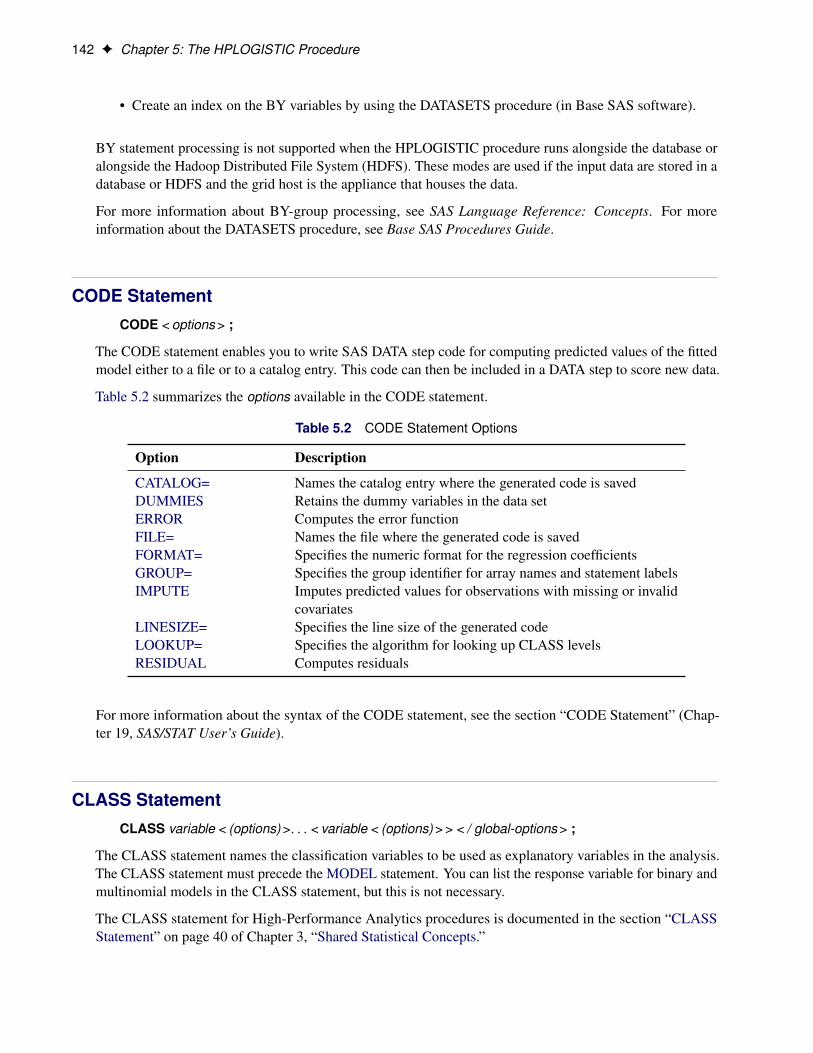
142 F Chapter 5: The HPLOGISTIC Procedure
• Create an index on the BY variables by using the DATASETS procedure (in Base SAS software).
BY statement processing is not supported when the HPLOGISTIC procedure runs alongside the database oralongside the Hadoop Distributed File System (HDFS). These modes are used if the input data are stored in adatabase or HDFS and the grid host is the appliance that houses the data.
For more information about BY-group processing, see SAS Language Reference: Concepts. For moreinformation about the DATASETS procedure, see Base SAS Procedures Guide.
CODE StatementCODE < options > ;
The CODE statement enables you to write SAS DATA step code for computing predicted values of the fittedmodel either to a file or to a catalog entry. This code can then be included in a DATA step to score new data.
Table 5.2 summarizes the options available in the CODE statement.
Table 5.2 CODE Statement Options
Option Description
CATALOG= Names the catalog entry where the generated code is savedDUMMIES Retains the dummy variables in the data setERROR Computes the error functionFILE= Names the file where the generated code is savedFORMAT= Specifies the numeric format for the regression coefficientsGROUP= Specifies the group identifier for array names and statement labelsIMPUTE Imputes predicted values for observations with missing or invalid
covariatesLINESIZE= Specifies the line size of the generated codeLOOKUP= Specifies the algorithm for looking up CLASS levelsRESIDUAL Computes residuals
For more information about the syntax of the CODE statement, see the section “CODE Statement” (Chap-ter 19, SAS/STAT User’s Guide).
CLASS StatementCLASS variable < (options) >: : : < variable < (options) > > < / global-options > ;
The CLASS statement names the classification variables to be used as explanatory variables in the analysis.The CLASS statement must precede the MODEL statement. You can list the response variable for binary andmultinomial models in the CLASS statement, but this is not necessary.
The CLASS statement for High-Performance Analytics procedures is documented in the section “CLASSStatement” on page 40 of Chapter 3, “Shared Statistical Concepts.”
FREQ Statement F 143
The HPLOGISTIC procedure does not support the SPLIT option in the CLASS statement. The HPLOGISTICprocedure additionally supports the following global-option in the CLASS statement:
UPCASEuppercases the values of character-valued CLASS variables before levelizing them. For example, if theUPCASE option is in effect and a CLASS variable can take the values ‘a’, ‘A’, and ‘b’, then ‘a’ and ‘A’represent the same level and the CLASS variable is treated as having only two values: ‘A’ and ‘B’.
FREQ StatementFREQ variable ;
The variable in the FREQ statement identifies a numeric variable in the data set that contains the frequency ofoccurrence for each observation. High-Performance Analytics procedures that support the FREQ statementtreat each observation as if it appeared f times, where the frequency value f is the value of the FREQvariable for the observation. If f is not an integer, then f is truncated to an integer. If f is less than 1or missing, the observation is not used in the analysis. When the FREQ statement is not specified, eachobservation is assigned a frequency of 1.
ID StatementID variables ;
The ID statement lists one or more variables from the input data set that are to be transferred to output datasets created by High-Performance Analytics procedures, provided that the output data set produces one (ormore) records per input observation.
For documentation about the common ID statement in High-Performance Analytics procedures, see thesection “ID Statement” on page 44 in Chapter 3, “Shared Statistical Concepts.”
MODEL StatementMODEL response < (response-options) > = < effects > < / model-options > ;
MODEL events / trials < (response-options) > = < effects > < / model-options > ;
The MODEL statement defines the statistical model in terms of a response variable (the target) or anevents/trials specification, model effects constructed from variables in the input data set, and options. Anintercept is included in the model by default. You can remove the intercept with the NOINT option.
You can specify a single response variable that contains your binary, ordinal, or nominal response values.When you have binomial data, you can specify the events/trials form of the response, where one variablecontains the number of positive responses (or events) and another variable contains the number of trials.Note that the values of both events and (trials – events) must be nonnegative and the value of trials must bepositive.
For information about constructing the model effects, see the section “Specification and Parameterization ofModel Effects” on page 52 of Chapter 3, “Shared Statistical Concepts.”
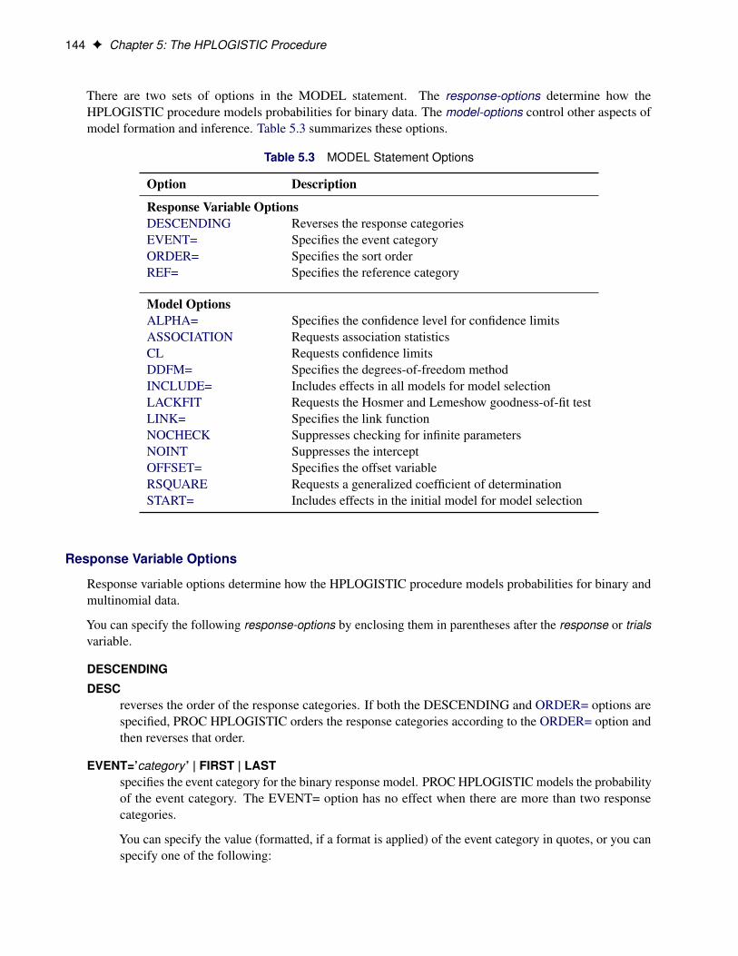
144 F Chapter 5: The HPLOGISTIC Procedure
There are two sets of options in the MODEL statement. The response-options determine how theHPLOGISTIC procedure models probabilities for binary data. The model-options control other aspects ofmodel formation and inference. Table 5.3 summarizes these options.
Table 5.3 MODEL Statement Options
Option Description
Response Variable OptionsDESCENDING Reverses the response categoriesEVENT= Specifies the event categoryORDER= Specifies the sort orderREF= Specifies the reference category
Model OptionsALPHA= Specifies the confidence level for confidence limitsASSOCIATION Requests association statisticsCL Requests confidence limitsDDFM= Specifies the degrees-of-freedom methodINCLUDE= Includes effects in all models for model selectionLACKFIT Requests the Hosmer and Lemeshow goodness-of-fit testLINK= Specifies the link functionNOCHECK Suppresses checking for infinite parametersNOINT Suppresses the interceptOFFSET= Specifies the offset variableRSQUARE Requests a generalized coefficient of determinationSTART= Includes effects in the initial model for model selection
Response Variable Options
Response variable options determine how the HPLOGISTIC procedure models probabilities for binary andmultinomial data.
You can specify the following response-options by enclosing them in parentheses after the response or trialsvariable.
DESCENDING
DESCreverses the order of the response categories. If both the DESCENDING and ORDER= options arespecified, PROC HPLOGISTIC orders the response categories according to the ORDER= option andthen reverses that order.
EVENT=’category ’ | FIRST | LASTspecifies the event category for the binary response model. PROC HPLOGISTIC models the probabilityof the event category. The EVENT= option has no effect when there are more than two responsecategories.
You can specify the value (formatted, if a format is applied) of the event category in quotes, or you canspecify one of the following:
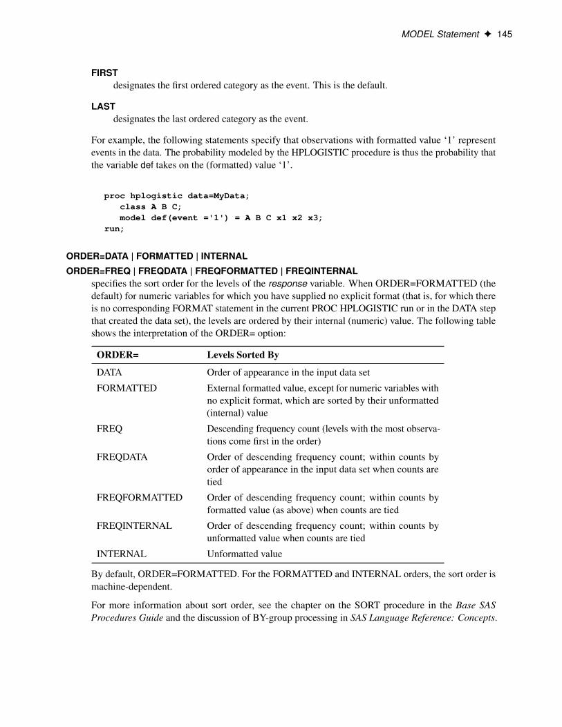
MODEL Statement F 145
FIRSTdesignates the first ordered category as the event. This is the default.
LASTdesignates the last ordered category as the event.
For example, the following statements specify that observations with formatted value ‘1’ representevents in the data. The probability modeled by the HPLOGISTIC procedure is thus the probability thatthe variable def takes on the (formatted) value ‘1’.
proc hplogistic data=MyData;class A B C;model def(event ='1') = A B C x1 x2 x3;
run;
ORDER=DATA | FORMATTED | INTERNAL
ORDER=FREQ | FREQDATA | FREQFORMATTED | FREQINTERNALspecifies the sort order for the levels of the response variable. When ORDER=FORMATTED (thedefault) for numeric variables for which you have supplied no explicit format (that is, for which thereis no corresponding FORMAT statement in the current PROC HPLOGISTIC run or in the DATA stepthat created the data set), the levels are ordered by their internal (numeric) value. The following tableshows the interpretation of the ORDER= option:
ORDER= Levels Sorted By
DATA Order of appearance in the input data set
FORMATTED External formatted value, except for numeric variables withno explicit format, which are sorted by their unformatted(internal) value
FREQ Descending frequency count (levels with the most observa-tions come first in the order)
FREQDATA Order of descending frequency count; within counts byorder of appearance in the input data set when counts aretied
FREQFORMATTED Order of descending frequency count; within counts byformatted value (as above) when counts are tied
FREQINTERNAL Order of descending frequency count; within counts byunformatted value when counts are tied
INTERNAL Unformatted value
By default, ORDER=FORMATTED. For the FORMATTED and INTERNAL orders, the sort order ismachine-dependent.
For more information about sort order, see the chapter on the SORT procedure in the Base SASProcedures Guide and the discussion of BY-group processing in SAS Language Reference: Concepts.

146 F Chapter 5: The HPLOGISTIC Procedure
REF=’category ’ | FIRST | LASTspecifies the reference category for the generalized logit model and the binary response model. For thegeneralized logit model, each logit contrasts a nonreference category with the reference category. Forthe binary response model, specifying one response category as the reference is the same as specifyingthe other response category as the event category. You can specify the value (formatted if a format isapplied) of the reference category in quotes, or you can specify one of the following:
FIRSTdesignates the first ordered category as the reference
LASTdesignates the last ordered category as the reference. This is the default.
Model Options
ALPHA=numberrequests that confidence intervals for each of the parameters be constructed with confidence level1–number. The value of number must be between 0 and 1; the default is 0.05.
ASSOCIATIONdisplays measures of association between predicted probabilities and observed responses. Thesemeasures assess the predictive ability of a model.
Of the n pairs of observations in the data set with different responses, let nc be the number of pairswhere the observation that has the lower ordered response value has a lower predicted probability,let nd be the number of pairs where the observation that has the lower ordered response value has ahigher predicted probability, and let nt D n � nc � nd be the rest. Let N be the sum of observationfrequencies in the data. Then the following statistics are reported:
concordance index C (AUC) D .nc C 0:5nt /=n
Somers’ D (Gini coefficient) D .nc � nd /=n
Goodman-Kruskal gamma D .nc � nd /=.nc C nd /
Kendall’s tau-a D .nc � nd /=.0:5N.N � 1//
Classification of the pairs is carried out by initially binning the predicted probabilities as discussed inthe section “The Hosmer-Lemeshow Goodness-of-Fit Test” on page 156. The concordance index, C, isan estimate of the AUC, which is the area under the receiver operating characteristic (ROC) curve.
CLrequests that confidence limits be constructed for each of the parameter estimates. The confidencelevel is 0.95 by default; this can be changed with the ALPHA= option.
DDFM=RESIDUAL | NONEspecifies how degrees of freedom for statistical inference be determined in the “Parameter EstimatesTable.”
The HPLOGISTIC procedure always displays the statistical tests and confidence intervals in the“Parameter Estimates” tables in terms of a t test and a two-sided probability from a t distribution.With the DDFM= option, you can control the degrees of freedom of this t distribution and therebyswitch between small-sample inference and large-sample inference based on the normal or chi-squaredistribution.

MODEL Statement F 147
The default is DDFM=NONE, which leads to z-based statistical tests and confidence intervals. TheHPLOGISTIC procedure then displays the degrees of freedom in the DF column as Infty, the p-valuesare identical to those from a Wald chi-square test, and the square of the t value equals the Waldchi-square statistic.
If you specify DDFM=RESIDUAL, the degrees of freedom are finite and determined by the number ofusable frequencies (observations) minus the number of nonredundant model parameters. This leads tot-based statistical tests and confidence intervals. If the number of frequencies is large relative to thenumber of parameters, the inferences from the two degrees-of-freedom methods are almost identical.
INCLUDE=n
INCLUDE=single-effect
INCLUDE=(effects)forces effects to be included in all models. If you specify INCLUDE=n, then the first n effects that arelisted in the MODEL statement are included in all models. If you specify INCLUDE=single-effect orif you specify a list of effects within parentheses, then the specified effects are forced into all models.The effects that you specify in the INCLUDE= option must be explanatory effects that are specified inthe MODEL statement before the slash (/).
LACKFIT< (DFREDUCE=r NGROUPS=G) >performs the Hosmer and Lemeshow goodness-of-fit test (Hosmer and Lemeshow 2000) for binaryresponse models.
The subjects are divided into at most G groups of roughly the same size, based on the percentiles ofthe estimated probabilities. You can specify G as any integer greater than or equal to 5; by default,G=10. Let the actual number of groups created be g. The discrepancies between the observed andexpected number of observations in these g groups are summarized by the Pearson chi-square statistic,which is then compared to a chi-square distribution with g–r degrees of freedom. You can specify anonnegative integer r that satisfies g–r � 1; by default, r=2.
A small p-value suggests that the fitted model is not an adequate model. See the section “TheHosmer-Lemeshow Goodness-of-Fit Test” on page 156 for more information.
LINK=keywordspecifies the link function for the model. The keywords and the associated link functions are shown inTable 5.4.
Table 5.4 Built-in Link Functions of the HPLOGISTIC Procedure
LinkLINK= Function g.�/ D � D
CLOGLOG | CLL Complementary log-log log.� log.1 � �//GLOGIT | GENLOGIT Generalized logitLOGIT Logit log.�=.1 � �//LOGLOG Log-log � log.� log.�//PROBIT Probit ˆ�1.�/
For the probit and cumulative probit links, ˆ�1.�/ denotes the quantile function of the standard normaldistribution.
148 F Chapter 5: The HPLOGISTIC Procedure
If the response variable has more than two categories, the HPLOGISTIC procedure fits a model with acumulative link function based on the specified link. However, if you specify LINK=GLOGIT, theprocedure assumes a generalized logit model for nominal (unordered) data, regardless of the numberof response categories.
NOCHECKdisables the checking process that determines whether maximum likelihood estimates of the regressionparameters exist. For more information, see the section “Existence of Maximum Likelihood Estimates”on page 154.
NOINTrequests that no intercept be included in the model. An intercept is included by default. The NOINToption is not available in multinomial models.
OFFSET=variablespecifies a variable to be used as an offset to the linear predictor. An offset plays the role of an effectwhose coefficient is known to be 1. The offset variable cannot appear in the CLASS statement orelsewhere in the MODEL statement. Observations with missing values for the offset variable areexcluded from the analysis.
RSQUARE
R2requests a generalized coefficient of determination (R square, R2) and a scaled version thereof forthe fitted model. The results are added to the “Fit Statistics” table. For more information aboutthe computation of these measures, see the section “Generalized Coefficient of Determination” onpage 155.
START=n
START=single-effect
START=(effects)begins the selection process from the designated initial model for the FORWARD and STEPWISEselection methods. If you specify START=n, then the starting model includes the first n effects thatare listed in the MODEL statement. If you specify START=single-effect or if you specify a list ofeffects within parentheses, then the starting model includes those specified effects. The effects that youspecify in the START= option must be explanatory effects that are specified in the MODEL statementbefore the slash (/). The START= option is not available when you specify METHOD=BACKWARDin the SELECTION statement.
OUTPUT StatementOUTPUT < OUT=SAS-data-set >
< keyword < =name > >. . . < keyword < =name > > < / options > ;
The OUTPUT statement creates a data set that contains observationwise statistics that are computed afterfitting the model. The variables in the input data set are not included in the output data set to avoid dataduplication for large data sets; however, variables specified in the ID statement or COPYVAR= option areincluded.

OUTPUT Statement F 149
If the input data are in distributed form, where access of data in a particular order cannot be guaranteed, theHPLOGISTIC procedure copies the distribution or partition key to the output data set so that its contents canbe joined with the input data.
The output statistics are computed based on the final parameter estimates. If the model fit does not converge,missing values are produced for the quantities that depend on the estimates.
When there are more than two response levels, only variables named by the XBETA and PREDICTEDkeywords have their values computed; the other variables have missing values. These statistics are computedfor every response category, and the automatic variable _LEVEL_ identifies the response category upon whichthe computed values are based. If you also specify the OBSCAT option, then the observationwise statisticsare computed only for the observed response category, as indicated by the value of the _LEVEL_ variable.
For observations in which only the response variable is missing, values of the XBETA and PREDICTEDstatistics are computed even though these observations do not affect the model fit. This enables, for instance,predicted probabilities to be computed for new observations.
You can specify the following syntax elements in the OUTPUT statement before the slash (/).
OUT=SAS-data-set
DATA=SAS-data-setspecifies the name of the output data set. If the OUT= (or DATA=) option is omitted, the procedureuses the DATAn convention to name the output data set.
keyword < =name >specifies a statistic to include in the output data set and optionally names the variable name. If you donot provide a name, the HPLOGISTIC procedure assigns a default name based on the type of statisticrequested.
The following are valid keywords for adding statistics to the OUTPUT data set:
LINP | XBETArequests the linear predictor � D x0ˇ.
PREDICTED | PRED | Prequests predicted values (predicted probabilities of events) for the response variable.
RESIDUAL | RESID | Rrequests the raw residual, y � �, where � is the estimate of the predicted event probability. Thisstatistic is not computed for multinomial models.
PEARSON | PEARS | RESCHIrequests the Pearson residual,
pwn.y=n��/p�.1��/
, where � is the estimate of the predicted eventprobability, w is the weight of the observation, and n is the number of binomial trials (n=1 forbinary observations). This statistic is not computed for multinomial models.
You can specify the following options in the OUTPUT statement after the slash (/):
COPYVAR=variable
COPYVAR=(variables)transfers one or more variables from the input data set to the output data set.
150 F Chapter 5: The HPLOGISTIC Procedure
OBSCATrequests (for multinomial models) that observationwise statistics be produced for the response levelonly. If the OBSCAT option is not specified and the response variable has J levels, then the followingoutputs are created: for cumulative link models, J � 1 records are output for every observation inthe input data that corresponds to the J � 1 lower-ordered response categories; for generalized logitmodels, J records are output that correspond to all J response categories.
PERFORMANCE StatementPERFORMANCE < performance-options > ;
The PERFORMANCE statement defines performance parameters for multithreaded and distributed comput-ing, passes variables about the distributed computing environment, and requests detailed results about theperformance characteristics of the HPLOGISTIC procedure.
With the PERFORMANCE statement you can also control whether the HPLOGISTIC procedure executes insingle-machine mode or distributed mode.
The PERFORMANCE statement for High-Performance Analytics procedures is documented in the section“PERFORMANCE Statement” on page 34
SELECTION StatementSELECTION < options > ;
The SELECTION statement performs model selection by examining whether effects should be added toor removed from the model according to rules defined by model selection methods. The statement is fullydocumented in the section “SELECTION Statement” on page 45 in Chapter 3, “Shared Statistical Concepts.”
The HPLOGISTIC procedure supports the following effect-selection methods in the SELECTION statement:
METHOD=NONE results in no model selection. This method fits the full model.
METHOD=FORWARD performs forward selection. This method starts with no effects in themodel and adds effects.
METHOD=BACKWARD performs backward elimination. This method starts with all effects in themodel and deletes effects.
METHOD=BACKWARD(FAST) performs fast backward elimination. This method starts with all effectsin the model and deletes effects without refitting the model.
METHOD=STEPWISE performs stepwise regression. This method is similar to the FORWARDmethod except that effects already in the model do not necessarily staythere.
The only effect-selection criterion supported by the HPLOGISTIC procedure is SELECT=SL, where effectsenter and leave the model based on an evaluation of the significance level. To determine this level ofsignificance for each candidate effect, the HPLOGISTIC procedure calculates an approximate chi-squarescore test statistic.
WEIGHT Statement F 151
The default criterion for the CHOOSE= and STOP= options in the SELECT statement is the significancelevel of the score test. The following criteria can be specified:
AIC Akaike’s information criterion (Akaike 1974)
AICC a small-sample bias corrected version of Akaike’s information criterionas promoted in, for example, Hurvich and Tsai (1989) and Burnham andAnderson (1998)
BIC | SBC Schwarz’ Bayesian criterion (Schwarz 1978)
SL the significance level of the score test (STOP= only)
The calculation of the information criteria uses the following formulas, where p denotes the number ofeffective parameters in the candidate model, f denotes the number of frequencies used, and l is the loglikelihood evaluated at the converged estimates:
AIC D� 2l C 2p
AICC D��2l C 2pf=.f � p � 1/ whenf > p C 2
�2l C 2p.p C 2/ otherwise
BIC D� 2l C p log.f /
NOTE: If you use the fast backward elimination method, the –2 log likelihood, AIC, AICC, and BIC statisticsare approximated at each step where the model is not refit, and hence do not match the values computedwhen that model is fit outside of the selection routine.
When you specify the DETAILS= option in the SELECTION statement, the HPLOGISTIC procedureproduces the following:
DETAILS=SUMMARY produces a summary table that shows the effect added or removed at eachstep along with the p-value. The summary table is produced by default ifthe DETAILS= option is not specified.
DETAILS=STEPS produces a detailed listing of all candidates at each step and their rankingin terms of the significance level for entry into or removal from the model.
DETAILS=ALL produces the preceding two tables and a table of selection details whichdisplays fit statistics for the model at each step of the selection processand the approximate chi-square score statistic.
WEIGHT StatementWEIGHT variable ;
The variable in the WEIGHT statement is used as a weight to perform a weighted analysis of the data.Observations with nonpositive or missing weights are not included in the analysis. If a WEIGHT statement isnot included, then all observations used in the analysis are assigned a weight of 1.
152 F Chapter 5: The HPLOGISTIC Procedure
Details: HPLOGISTIC Procedure
Missing ValuesAny observation with missing values for the response, frequency, weight, offset, or explanatory variables isexcluded from the analysis; however, missing values are valid for response and explanatory variables that arespecified with the MISSING option in the CLASS statement. Observations with a nonpositive weight or witha frequency less than 1 are also excluded.
The estimated linear predictor and the fitted probabilities are not computed for any observation that hasmissing offset or explanatory variable values. However, if only the response value is missing, the linearpredictor and the fitted probabilities can be computed and output to a data set by using the OUTPUTstatement.
Response DistributionsThe response distribution is the probability distribution of the response (target) variable. The HPLOGISTICprocedure can fit data for the following distributions:
• binary distribution
• binomial distribution
• multinomial distribution
The expressions for the log-likelihood functions of these distributions are given in the next section.
The binary (or Bernoulli) distribution is the elementary distribution of a discrete random variable that cantake on two values with probabilities p and 1 � p. Suppose the random variable is denoted Y and
Pr.Y D 1/ D pPr.Y D 0/ D 1 � p
The value associated with probability p is often termed the event or “success”; the complementary event istermed the non-event or “failure.” A Bernoulli experiment is a random draw from a binary distribution andgenerates events with probability p.
If Y1; � � � ; Yn are n independent Bernoulli random variables, then their sum follows a binomial distribution.In other words, if Yi D 1 denotes an event (success) in the i th Bernoulli trial, a binomial random variable isthe number of events (successes) in n independent Bernoulli trials. If you use the events/trials syntax in theMODEL statement, the HPLOGISTIC procedure fits the model as if the data had arisen from a binomialdistribution. For example, the following statements fit a binomial regression model with regressors x1 and x2.The variables e and t represent the events and trials for the binomial distribution:
Log-Likelihood Functions F 153
proc hplogistic;model e/t = x1 x2;
run;
If the events/trials syntax is used, then both variables must be numeric and the value of the events variablecannot be less than 0 or exceed the value of the trials variable. A “Response Profile” table is not produced forbinomial data, since the response variable is not subject to levelization.
The multinomial distribution is a generalization of the binary distribution and allows for more than twooutcome categories. Because there are more than two possible outcomes for the multinomial distribution, theterminology of “successes,” “failures,” “events,” and “non-events” no longer applies. With multinomial data,these outcomes are generically referred to as “categories” or levels.
Whenever the HPLOGISTIC procedure determines that the response variable has more than two levels (unlessthe events/trials syntax is used), the procedure fits the model as if the data had arisen from a multinomialdistribution. By default, it is then assumed that the response categories are ordered and a cumulative linkmodel is fit by applying the default or specified link function. If the response categories are unordered, thenyou should fit a generalized logit model by choosing LINK=GLOGIT in the MODEL statement.
Log-Likelihood FunctionsThe HPLOGISTIC procedure forms the log-likelihood functions of the various models as
L.�I y/ DnXiD1
fi l.�i Iyi ; wi /
where l.�i Iyi ; wi / is the log-likelihood contribution of the i th observation with weight wi and fi is thevalue of the frequency variable. For the determination of wi and fi , see the WEIGHT and FREQ statements.The individual log-likelihood contributions for the various distributions are as follows.
Binary Distribution
The HPLOGISTIC procedure computes the log-likelihood function l.�i .ˇ/Iyi / for the i th binary observationas
�i D x0iˇ
�i .ˇ/ D g�1.�i /
l.�i .ˇ/Iyi / D yi logf�ig C .1 � yi / logf1 � �ig
Here, �i is the probability of an event, and the variable yi takes on the value 1 for an event and the value 0for a non-event. The inverse link function g�1.�/ maps from the scale of the linear predictor �i to the scale ofthe mean. For example, for the logit link (the default),
�i .ˇ/ Dexpf�ig
1C expf�ig
You can control which binary outcome in your data is modeled as the event with the response-options in theMODEL statement, and you can choose the link function with the LINK= option in the MODEL statement.
154 F Chapter 5: The HPLOGISTIC Procedure
If a WEIGHT statement is given and wi denotes the weight for the current observation, the log-likelihoodfunction is computed as
l.�i .ˇ/Iyi ; wi / D wi l.�i .ˇ/Iyi /
Binomial Distribution
The HPLOGISTIC procedure computes the log-likelihood function l.�i .ˇ/Iyi / for the i th binomial obser-vation as
�i D x0iˇ
�i .ˇ/ D g�1.�i /
l.�i .ˇ/Iyi ; wi / D wi .yi logf�ig C .ni � yi / logf1 � �ig/C wi .logf�.ni C 1/g � logf�.yi C 1/g � logf�.ni � yi C 1/g/
where yi and ni are the values of the events and trials of the i th observation, respectively. �i measuresthe probability of events (successes) in the underlying Bernoulli distribution whose aggregate follows thebinomial distribution.
Multinomial Distribution
The multinomial distribution modeled by the HPLOGISTIC procedure is a generalization of the binarydistribution; it is the distribution of a single draw from a discrete distribution with J possible values. Thelog-likelihood function for the i th observation is thus deceptively simple:
l.�i I yi ; wi / D wiJXjD1
yij logf�ij g
In this expression, J denotes the number of response categories (the number of possible outcomes) and �ij isthe probability that the i th observation takes on the response value associated with category j . The categoryprobabilities must satisfy
JXjD1
�j D 1
and the constraint is satisfied by modeling J � 1 categories. In models with ordered response categories, theprobabilities are expressed in cumulative form, so that the last category is redundant. In generalized logitmodels (multinomial models with unordered categories), one category is chosen as the reference categoryand the linear predictor in the reference category is set to zero.
Existence of Maximum Likelihood EstimatesThe likelihood equation for a logistic regression model does not always have a finite solution. Sometimesthere is a nonunique maximum on the boundary of the parameter space, at infinity. The existence, finiteness,and uniqueness of maximum likelihood estimates for the logistic regression model depend on the patterns ofdata points in the observation space (Albert and Anderson 1984; Santner and Duffy 1986).
Generalized Coefficient of Determination F 155
Consider a binary response model. Let Yj be the response of the jth subject, and let xj be the vector ofexplanatory variables (including the constant 1 that is associated with the intercept). There are three mutuallyexclusive and exhaustive types of data configurations: complete separation, quasi-complete separation, andoverlap.
Complete Separation There is a complete separation of data points if there exists a vector b that correctlyallocates all observations to their response groups; that is,�
b0xj > 0 Yj D 1
b0xj < 0 Yj D 2
This configuration produces nonunique infinite estimates. If the iterative process of maximizingthe likelihood function is allowed to continue, the log likelihood diminishes to 0, and the dispersionmatrix becomes unbounded.
Quasi-complete Separation The data are not completely separable, but there is a vector b such that�b0xj � 0 Yj D 1
b0xj � 0 Yj D 2
and equality holds for at least one subject in each response group. This configuration also yieldsnonunique infinite estimates. If the iterative process of maximizing the likelihood function isallowed to continue, the dispersion matrix becomes unbounded and the log likelihood diminishesto a nonzero constant.
Overlap If neither complete nor quasi-complete separation exists in the sample points, there is an overlapof sample points. In this configuration, the maximum likelihood estimates exist and are unique.
The HPLOGISTIC procedure uses a simple empirical approach to recognize the data configurations that leadto infinite parameter estimates. The basis of this approach is that any convergence method of maximizingthe log likelihood must yield a solution that indicates complete separation, if such a solution exists. Uponconvergence, if the predicted response equals the observed response for every observation, there is a completeseparation of data points.
If the data are not completely separated, if an observation is identified to have an extremely large probability(� 0.95) of predicting the observed response, and if there have been at least eight iterations, then there aretwo possible situations. First, there is overlap in the data set, the observation is an atypical observation of itsown group, and the iterative process stopped when a maximum was reached. Second, there is quasi-completeseparation in the data set, and the asymptotic dispersion matrix is unbounded. If any of the diagonal elementsof the dispersion matrix for the standardized observation vector (all explanatory variables standardized to zeromean and unit variance) exceeds 5,000, quasi-complete separation is declared. If either complete separationor quasi-complete separation is detected, a note is displayed in the procedure output.
Checking for quasi-complete separation is less foolproof than checking for complete separation. If neithertype of separation is discovered and your parameter estimates have large standard errors, then this indicatesthat your data might be separable. The NOCHECK option in the MODEL statement turns off the process ofchecking for infinite parameter estimates.
Generalized Coefficient of DeterminationThe goal of a coefficient of determination, also known as an R-square measure, is to express the agreementbetween a stipulated model and the data in terms of variation in the data explained by the model. In linear
156 F Chapter 5: The HPLOGISTIC Procedure
models, the R-square measure is based on residual sums of squares; because these are additive, a measurebounded between 0 and 1 is easily derived.
In more general models where parameters are estimated by the maximum likelihood principle, Cox andSnell (1989, pp. 208–209) and Magee (1990) proposed the following generalization of the coefficient ofdetermination:
R2 D 1 �
�L.0/
L.b/� 2n
Here, L.0/ is the likelihood of the intercept-only model, L.b/ is the likelihood of the specified model, and ndenotes the number of observations used in the analysis. This number is adjusted for frequencies if a FREQstatement is present and is based on the trials variable for binomial models.
As discussed in Nagelkerke (1991), this generalized R-square measure has properties similar to the coefficientof determination in linear models. If the model effects do not contribute to the analysis, L.b/ approachesL.0/ and R2 approaches zero.
However, R2 does not have an upper limit of 1. Nagelkerke suggested a rescaled generalized coefficient ofdetermination that achieves an upper limit of 1, by dividing R2 by its maximum value,
R2max D 1 � fL.0/g2n
If you specify the RSQUARE option in the MODEL statement, the HPLOGISTIC procedure computes R2
and the rescaled coefficient of determination according to Nagelkerke:
QR2 DR2
R2max
The R2 and QR2 measures are most useful for comparing competing models that are not necessarily nested—that is, models that cannot be reduced to one another by simple constraints on the parameter space. Largervalues of the measures indicate better models.
The Hosmer-Lemeshow Goodness-of-Fit TestTo evaluate the fit of the model, Hosmer and Lemeshow (2000) proposed a statistic that they show, throughsimulation, is distributed as chi-square when there is no replication in any of the subpopulations. Thisgoodness-of-fit test is available only for binary response models.
The unit interval is partitioned into 2,000 equal-sized bins, and each observation i is placed into the bin thatcontains its estimated event probability. This effectively sorts the observations in increasing order of theirestimated event probability.
The observations (and frequencies) are further combined into G groups. By default G=10, but you canspecify G � 5 with the NGROUPS= suboption of the LACKFIT option in the MODEL statement. Let F bethe total frequency. The target frequency for each group is T D bF=G C 0:5c, which is the integer part ofF=G C 0:5. Load the first group (gj ; j D 1) with the first of the 2,000 bins that has nonzero frequency f1,and let the next nonzero bin have a frequency of f . PROC HPLOGISTIC performs the following steps foreach nonzero bin to create the groups:
Computational Method: Multithreading F 157
1. If j D G, then add this bin to group gj .
2. Otherwise, if fj < T and fj C bf=2c � T , then add this bin to group gj .
3. Otherwise, start loading the next group (gjC1) with fjC1 D f , and set j D j C 1.
If the final group gj has frequency fj < T=2, then add these observations to the preceding group. The totalnumber of groups actually created, g, can be less than G.
The Hosmer-Lemeshow goodness-of-fit statistic is obtained by calculating the Pearson chi-square statisticfrom the 2 � g table of observed and expected frequencies. The statistic is written
�2HL D
gXjD1
.Oj � Fj N�j /2
Fj N�j .1 � N�j /
where, for the j th group gj , Fj DPi2gj
fi is the total frequency of subjects, Oj is the total frequencyof event outcomes, and N�j D
Pi2gj
fi bpi=Fj is the average estimated predicted probability of an eventoutcome. Let � be the square root of the machine epsilon divided by 4,000, which is about 2.5E–12. AnyN�j < � is set to �; similarly, any N�j > 1 � � is set to 1 � �.
The Hosmer-Lemeshow statistic is compared to a chi-square distribution with g � r degrees of freedom.You can specify r with the DFREDUCE= suboption of the LACKFIT option in the MODEL statement. Bydefault, r D 2, and to compute the Hosmer-Lemeshow statistic you must have g � r � 1. Large values of�2HL (and small p-values) indicate a lack of fit of the model.
Computational Method: MultithreadingThreading refers to the organization of computational work into multiple tasks (processing units that canbe scheduled by the operating system). A task is associated with a thread. Multithreading refers to theconcurrent execution of threads. When multithreading is possible, substantial performance gains can berealized compared to sequential (single-threaded) execution.
The number of threads spawned by the HPLOGISTIC procedure is determined by the number of CPUs on amachine and can be controlled by specifying the NTHREADS= option in the PERFORMANCE statement.This specification overrides the system option. Specify NTHREADS=1 to force single-threaded execution.The number of threads per machine is displayed in the “Dimensions” table, which is part of the default output.The HPLOGISTIC procedure allocates one thread per CPU by default.
The tasks that are multithreaded by the HPLOGISTIC procedure are primarily defined by dividing thedata processed on a single machine among the threads—that is, the HPLOGISTIC procedure implementsmultithreading through a data-parallel model. For example, if the input data set has 1,000 observations andyou are running with four threads, then 250 observations are associated with each thread. All operations thatrequire access to the data are then multithreaded. These operations include the following:
• variable levelization
• effect levelization
• formation of the initial crossproducts matrix
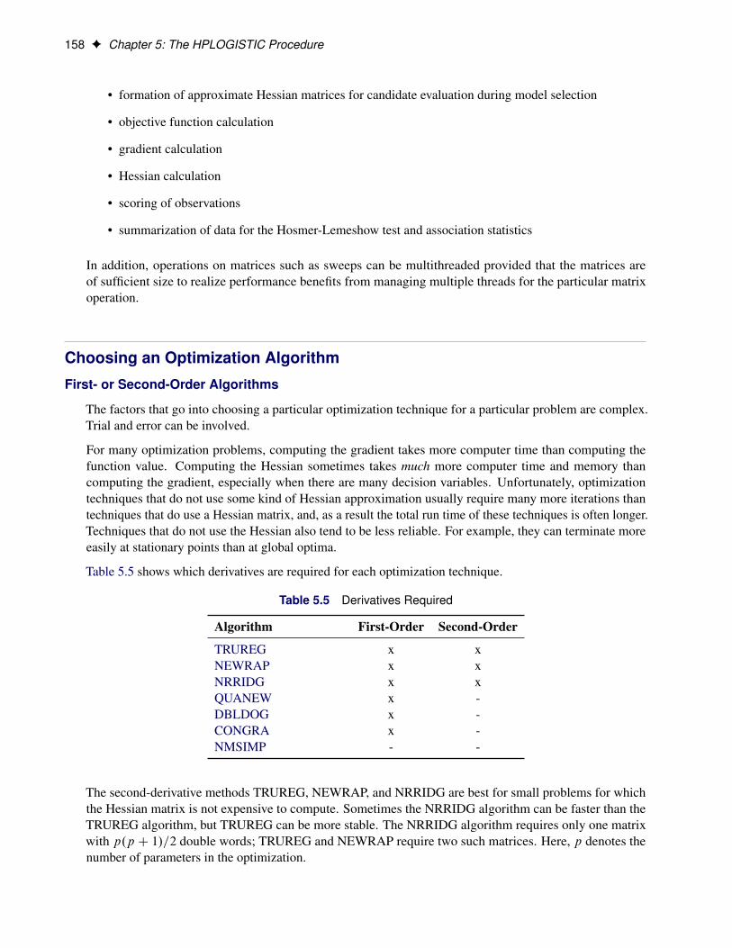
158 F Chapter 5: The HPLOGISTIC Procedure
• formation of approximate Hessian matrices for candidate evaluation during model selection
• objective function calculation
• gradient calculation
• Hessian calculation
• scoring of observations
• summarization of data for the Hosmer-Lemeshow test and association statistics
In addition, operations on matrices such as sweeps can be multithreaded provided that the matrices areof sufficient size to realize performance benefits from managing multiple threads for the particular matrixoperation.
Choosing an Optimization Algorithm
First- or Second-Order Algorithms
The factors that go into choosing a particular optimization technique for a particular problem are complex.Trial and error can be involved.
For many optimization problems, computing the gradient takes more computer time than computing thefunction value. Computing the Hessian sometimes takes much more computer time and memory thancomputing the gradient, especially when there are many decision variables. Unfortunately, optimizationtechniques that do not use some kind of Hessian approximation usually require many more iterations thantechniques that do use a Hessian matrix, and, as a result the total run time of these techniques is often longer.Techniques that do not use the Hessian also tend to be less reliable. For example, they can terminate moreeasily at stationary points than at global optima.
Table 5.5 shows which derivatives are required for each optimization technique.
Table 5.5 Derivatives Required
Algorithm First-Order Second-Order
TRUREG x xNEWRAP x xNRRIDG x xQUANEW x -DBLDOG x -CONGRA x -NMSIMP - -
The second-derivative methods TRUREG, NEWRAP, and NRRIDG are best for small problems for whichthe Hessian matrix is not expensive to compute. Sometimes the NRRIDG algorithm can be faster than theTRUREG algorithm, but TRUREG can be more stable. The NRRIDG algorithm requires only one matrixwith p.p C 1/=2 double words; TRUREG and NEWRAP require two such matrices. Here, p denotes thenumber of parameters in the optimization.
Choosing an Optimization Algorithm F 159
The first-derivative methods QUANEW and DBLDOG are best for medium-sized problems for which theobjective function and the gradient can be evaluated much faster than the Hessian. In general, the QUANEWand DBLDOG algorithms require more iterations than TRUREG, NRRIDG, and NEWRAP, but each iterationcan be much faster. The QUANEW and DBLDOG algorithms require only the gradient to update anapproximate Hessian, and they require slightly less memory than TRUREG or NEWRAP.
The first-derivative method CONGRA is best for large problems for which the objective function and thegradient can be computed much faster than the Hessian and for which too much memory is required to storethe (approximate) Hessian. In general, the CONGRA algorithm requires more iterations than QUANEW orDBLDOG, but each iteration can be much faster. Because CONGRA requires only a factor of p double-wordmemory, many large applications can be solved only by CONGRA.
The no-derivative method NMSIMP is best for small problems for which derivatives are not continuous orare very difficult to compute.
Each optimization method uses one or more convergence criteria that determine when it has converged. Analgorithm is considered to have converged when any one of the convergence criteria is satisfied. For example,under the default settings, the QUANEW algorithm converges if ABSGCONV < 1E–5, FCONV < 2 � �, orGCONV < 1E–8.
By default, the HPLOGISTIC procedure applies the NRRIDG algorithm because it can take advantageof multithreading in Hessian computations and inversions. If the number of parameters becomes large,specifying the TECHNIQUE=QUANEW option, which is a first-order method with good overall properties,is recommended.
Algorithm Descriptions
The following subsections provide details about each optimization technique and follow the same order asTable 5.5.
Trust Region Optimization (TRUREG)The trust region method uses the gradient g. .k// and the Hessian matrix H. .k//; thus, it requires that theobjective function f . / have continuous first- and second-order derivatives inside the feasible region.
The trust region method iteratively optimizes a quadratic approximation to the nonlinear objective functionwithin a hyperelliptic trust region with radius � that constrains the step size that corresponds to the quality ofthe quadratic approximation. The trust region method is implemented based on Dennis, Gay, and Welsch(1981), Gay (1983), and Moré and Sorensen (1983).
The trust region method performs well for small- to medium-sized problems, and it does not need manyfunction, gradient, and Hessian calls. However, if the computation of the Hessian matrix is computationallyexpensive, one of the dual quasi-Newton or conjugate gradient algorithms might be more efficient.
Newton-Raphson Optimization with Line Search (NEWRAP)The NEWRAP technique uses the gradient g. .k// and the Hessian matrix H. .k//; thus, it requires thatthe objective function have continuous first- and second-order derivatives inside the feasible region. Ifsecond-order derivatives are computed efficiently and precisely, the NEWRAP method can perform well formedium-sized to large problems, and it does not need many function, gradient, and Hessian calls.
This algorithm uses a pure Newton step when the Hessian is positive-definite and when the Newton stepreduces the value of the objective function successfully. Otherwise, a combination of ridging and line search

160 F Chapter 5: The HPLOGISTIC Procedure
is performed to compute successful steps. If the Hessian is not positive-definite, a multiple of the identitymatrix is added to the Hessian matrix to make it positive-definite (Eskow and Schnabel 1991).
In each iteration, a line search is performed along the search direction to find an approximate optimum of theobjective function. The line-search method uses quadratic interpolation and cubic extrapolation.
Newton-Raphson Ridge Optimization (NRRIDG)The NRRIDG technique uses the gradient g. .k// and the Hessian matrix H. .k//; thus, it requires that theobjective function have continuous first- and second-order derivatives inside the feasible region.
This algorithm uses a pure Newton step when the Hessian is positive-definite and when the Newton stepreduces the value of the objective function successfully. If at least one of these two conditions is not satisfied,a multiple of the identity matrix is added to the Hessian matrix.
Because the NRRIDG technique uses an orthogonal decomposition of the approximate Hessian, each iterationof NRRIDG can be slower than that of the NEWRAP technique, which works with a Cholesky decomposition.However, NRRIDG usually requires fewer iterations than NEWRAP.
The NRRIDG method performs well for small- to medium-sized problems, and it does not require manyfunction, gradient, and Hessian calls. However, if the computation of the Hessian matrix is computationallyexpensive, one of the dual quasi-Newton or conjugate gradient algorithms might be more efficient.
Quasi-Newton Optimization (QUANEW)The dual quasi-Newton method uses the gradient g. .k//, and it does not need to compute second-orderderivatives because they are approximated. It works well for medium-sized to moderately large optimizationproblems, where the objective function and the gradient can be computed much faster than the Hessian.However, in general the QUANEW technique requires more iterations than the TRUREG, NEWRAP, andNRRIDG techniques, which compute second-order derivatives. The QUANEW technique provides anappropriate balance between the speed and stability required for most nonlinear mixed model applications.
The QUANEW technique implemented by the HPLOGISTIC procedure is the dual quasi-Newton algorithm,which updates the Cholesky factor of an approximate Hessian.
In each iteration, a line search is performed along the search direction to find an approximate optimum. Theline-search method uses quadratic interpolation and cubic extrapolation to obtain a step size ˛ that satisfiesthe Goldstein conditions (Fletcher 1987). One of the Goldstein conditions can be violated if the feasibleregion defines an upper limit of the step size. Violating the left-side Goldstein condition can affect thepositive-definiteness of the quasi-Newton update. In that case, either the update is skipped or the iterationsare restarted with an identity matrix, resulting in the steepest descent or ascent search direction.
Double-Dogleg Optimization (DBLDOG)The double-dogleg optimization method combines the ideas of the quasi-Newton and trust region methods.In each iteration, the double-dogleg algorithm computes the step s.k/ as the linear combination of the steepestdescent or ascent search direction s.k/1 and a quasi-Newton search direction s.k/2 :
s.k/ D ˛1s.k/1 C ˛2s
.k/2
The step is requested to remain within a prespecified trust region radius (Fletcher 1987, p. 107). Thus, theDBLDOG subroutine uses the dual quasi-Newton update but does not perform a line search.
The double-dogleg optimization technique works well for medium-sized to moderately large optimizationproblems, where the objective function and the gradient can be computed much faster than the Hessian.

Displayed Output F 161
The implementation is based on Dennis and Mei (1979) and Gay (1983), but it is extended for dealingwith boundary and linear constraints. The DBLDOG technique generally requires more iterations than theTRUREG, NEWRAP, and NRRIDG techniques, which require second-order derivatives; however, each of theDBLDOG iterations is computationally cheap. Furthermore, the DBLDOG technique requires only gradientcalls for the update of the Cholesky factor of an approximate Hessian.
Conjugate Gradient Optimization (CONGRA)Second-order derivatives are not required by the CONGRA algorithm and are not even approximated. TheCONGRA algorithm can be expensive in function and gradient calls, but it requires only O.p/ memory forunconstrained optimization. In general, many iterations are required to obtain a precise solution, but each ofthe CONGRA iterations is computationally cheap.
The CONGRA subroutine should be used for optimization problems with large p. For the unconstrainedor boundary-constrained case, CONGRA requires only O.p/ bytes of working memory, whereas all otheroptimization methods require order O.p2/ bytes of working memory. During p successive iterations,uninterrupted by restarts or changes in the working set, the conjugate gradient algorithm computes a cycleof p conjugate search directions. In each iteration, a line search is performed along the search direction tofind an approximate optimum of the objective function. The line-search method uses quadratic interpolationand cubic extrapolation to obtain a step size ˛ that satisfies the Goldstein conditions. One of the Goldsteinconditions can be violated if the feasible region defines an upper limit for the step size.
Nelder-Mead Simplex Optimization (NMSIMP)The Nelder-Mead simplex method does not use any derivatives and does not assume that the objectivefunction has continuous derivatives. The objective function itself needs to be continuous. This technique isquite expensive in the number of function calls, and it might be unable to generate precise results for p � 40.
The original Nelder-Mead simplex algorithm is implemented and extended to boundary constraints. Thisalgorithm does not compute the objective for infeasible points, but it changes the shape of the simplexadapting to the nonlinearities of the objective function. This change contributes to an increased speed ofconvergence and uses a special termination criterion.
Displayed OutputThe following sections describe the output that PROC HPLOGISTIC produces. The output is organized intovarious tables, which are discussed in the order of appearance.
Performance Information
The “Performance Information” table is produced by default. It displays information about the executionmode. For single-machine mode, the table displays the number of threads used. For distributed mode, thetable displays the grid mode (symmetric or asymmetric), the number of compute nodes, and the number ofthreads per node.
If you specify the DETAILS option in the PERFORMANCE statement, the procedure also produces a“Timing” table in which elapsed time (absolute and relative) for the main tasks of the procedure are displayed.
162 F Chapter 5: The HPLOGISTIC Procedure
Model Information
The “Model Information” table displays basic information about the model, such as the response variable,frequency variable, link function, and the model category the HPLOGISTIC procedure determined basedon your input and options. The “Model Information” table also displays the distribution of the data that isassumed by the HPLOGISTIC procedure. See the section “Response Distributions” on page 152 for how theprocedure determines the response distribution.
Class Level Information
The “Class Level Information” table lists the levels of every variable specified in the CLASS statement.You should check this information to make sure that the data are correct. You can adjust the order of theCLASS variable levels with the ORDER= option in the CLASS statement. You can suppress the “ClassLevel Information” table completely or partially with the NOCLPRINT= option in the PROC HPLOGISTICstatement.
If the classification variables use reference parameterization, the “Class Level Information” table also displaysthe reference value for each variable.
Number of Observations
The “Number of Observations” table displays the number of observations read from the input data set and thenumber of observations used in the analysis. If a FREQ statement is present, the sum of the frequencies readand used is displayed. If the events/trials syntax is used, the number of events and trials is also displayed.
Response Profile
The “Response Profile” table displays the ordered value from which the HPLOGISTIC procedure determinesthe probability being modeled as an event in binary models and the ordering of categories in multinomialmodels. For each response category level, the frequency used in the analysis is reported. You can affectthe ordering of the response values with the response-options in the MODEL statement. For binary andgeneralized logit models, the note that follows the “Response Profile” table indicates which outcome ismodeled as the event in binary models and which value serves as the reference category.
The “Response Profile” table is not produced for binomial data. You can find information about the numberof events and trials in the “Number of Observations” table.
Selection Information
When you specify the SELECTION statement, the HPLOGISTIC procedure produces by default a series oftables with information about the model selection. The “Selection Information” table informs you about themodel selection method, selection and stop criteria, and other parameters that govern the selection. You cansuppress this table by specifying DETAILS=NONE in the SELECTION statement.
Selection Summary
When you specify the SELECTION statement, the HPLOGISTIC procedure produces the “Selection Sum-mary” table with information about which effects were entered into or removed from the model at the stepsof the model selection process. The p-value for the score chi-square test that led to the removal or entrydecision is also displayed. You can request further details about the model selection steps by specifying
Displayed Output F 163
DETAILS=STEPS or DETAILS=ALL in the SELECTION statement. You can suppress the display of the“Selection Summary” table by specifying DETAILS=NONE in the SELECTION statement.
Stop Reason
When you specify the SELECTION statement, the HPLOGISTIC procedure produces a simple table thattells you why model selection stopped.
Selection Reason
When you specify the SELECTION statement, the HPLOGISTIC procedure produces a simple table thattells you why the final model was selected.
Selected Effects
When you specify the SELECTION statement, the HPLOGISTIC procedure produces a simple table thattells you which effects were selected into the final model.
Iteration History
For each iteration of the optimization, the “Iteration History” table displays the number of function evaluations(including gradient and Hessian evaluations), the value of the objective function, the change in the objectivefunction from the previous iteration and the absolute value of the largest (projected) gradient element. Theobjective function used in the optimization in the HPLOGISTIC procedure is normalized by default to enablecomparisons across data sets with different sampling intensity. You can control normalization with theNORMALIZE= option in the PROC HPLOGISTIC statement.
If you specify the ITDETAILS option in the PROC HPLOGISTIC statement, information about the parameterestimates and gradients in the course of the optimization is added to the “Iteration History” table.
The “Iteration History” table is displayed by default unless you specify the NOITPRINT option or perform amodel selection. To generate the history from a model selection process, specify the ITSELECT option.
Convergence Status
The convergence status table is a small ODS table that follows the “Iteration History” table in the defaultoutput. In the listing it appears as a message that indicates whether the optimization succeeded and whichconvergence criterion was met. If the optimization fails, the message indicates the reason for the failure. Ifyou save the convergence status table to an output data set, a numeric Status variable is added that enablesyou to assess convergence programmatically. The values of the Status variable encode the following:
0 Convergence was achieved, or an optimization was not performed (because TECHNIQUE=NONEis specified).
1 The objective function could not be improved.
2 Convergence was not achieved because of a user interrupt or because a limit was exceeded,such as the maximum number of iterations or the maximum number of function evaluations. Tomodify these limits, see the MAXITER=, MAXFUNC=, and MAXTIME= options in the PROCHPLOGISTIC statement.
164 F Chapter 5: The HPLOGISTIC Procedure
3 Optimization failed to converge because function or derivative evaluations failed at the startingvalues or during the iterations or because a feasible point that satisfies the parameter constraintscould not be found in the parameter space.
Dimensions
The “Dimensions” table displays size measures that are derived from the model and the environment. Forexample, it displays the number of columns in the design matrix, the rank of the matrix, the largest number ofdesign columns associated with an effect, the number of compute nodes in distributed mode, and the numberof threads per node.
Fit Statistics
The “Fit Statistics” table displays a variety of likelihood-based measures of fit. All statistics are presented in“smaller is better” form.
The calculation of the information criteria uses the following formulas, where p denotes the number ofeffective parameters, f denotes the number of frequencies used, and l is the log likelihood evaluated at theconverged estimates:
AIC D� 2l C 2p
AICC D��2l C 2pf=.f � p � 1/ whenf > p C 2
�2l C 2p.p C 2/ otherwise
BIC D� 2l C p log.f /
If no FREQ statement is given, f equals n, the number of observations used.
The values displayed in the “Fit Statistics” table are not based on a normalized log-likelihood function.
Global Tests
The “Global Tests” table provides a statistical test for the hypothesis of whether the final model provides abetter fit than a model without effects (an “intercept-only” model).
If you specify the NOINT option in the MODEL statement, the reference model is one where the linearpredictor is 0 for all observations.
Partition for the Hosmer and Lemeshow Test
The “Partition for the Hosmer and Lemeshow Test” table displays the grouping used in the Hosmer-Lemeshowtest. This table is displayed if you specify the LACKFIT option in the MODEL statement. See the section“The Hosmer-Lemeshow Goodness-of-Fit Test” on page 156 for details, and see Hosmer and Lemeshow(2000) for examples of using this partition.
Hosmer and Lemeshow Goodness-of-Fit Test
The “Hosmer and Lemeshow Goodness-of-Fit Test” table provides a test of the fit of the model; smallp-values reject the null hypothesis that the fitted model is adequate. This table is displayed if you specify theLACKFIT option in the MODEL statement. See the section “The Hosmer-Lemeshow Goodness-of-Fit Test”on page 156 for further details.
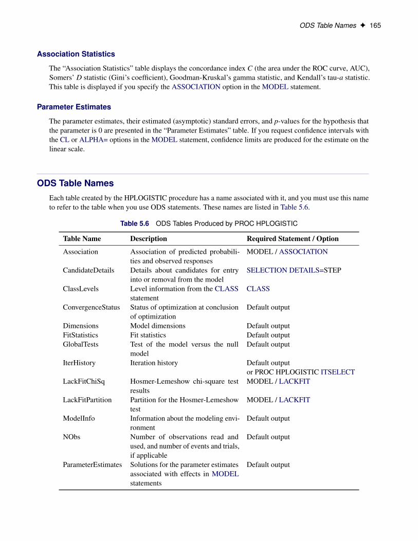
ODS Table Names F 165
Association Statistics
The “Association Statistics” table displays the concordance index C (the area under the ROC curve, AUC),Somers’ D statistic (Gini’s coefficient), Goodman-Kruskal’s gamma statistic, and Kendall’s tau-a statistic.This table is displayed if you specify the ASSOCIATION option in the MODEL statement.
Parameter Estimates
The parameter estimates, their estimated (asymptotic) standard errors, and p-values for the hypothesis thatthe parameter is 0 are presented in the “Parameter Estimates” table. If you request confidence intervals withthe CL or ALPHA= options in the MODEL statement, confidence limits are produced for the estimate on thelinear scale.
ODS Table NamesEach table created by the HPLOGISTIC procedure has a name associated with it, and you must use this nameto refer to the table when you use ODS statements. These names are listed in Table 5.6.
Table 5.6 ODS Tables Produced by PROC HPLOGISTIC
Table Name Description Required Statement / Option
Association Association of predicted probabili-ties and observed responses
MODEL / ASSOCIATION
CandidateDetails Details about candidates for entryinto or removal from the model
SELECTION DETAILS=STEP
ClassLevels Level information from the CLASSstatement
CLASS
ConvergenceStatus Status of optimization at conclusionof optimization
Default output
Dimensions Model dimensions Default outputFitStatistics Fit statistics Default outputGlobalTests Test of the model versus the null
modelDefault output
IterHistory Iteration history Default outputor PROC HPLOGISTIC ITSELECT
LackFitChiSq Hosmer-Lemeshow chi-square testresults
MODEL / LACKFIT
LackFitPartition Partition for the Hosmer-Lemeshowtest
MODEL / LACKFIT
ModelInfo Information about the modeling envi-ronment
Default output
NObs Number of observations read andused, and number of events and trials,if applicable
Default output
ParameterEstimates Solutions for the parameter estimatesassociated with effects in MODELstatements
Default output
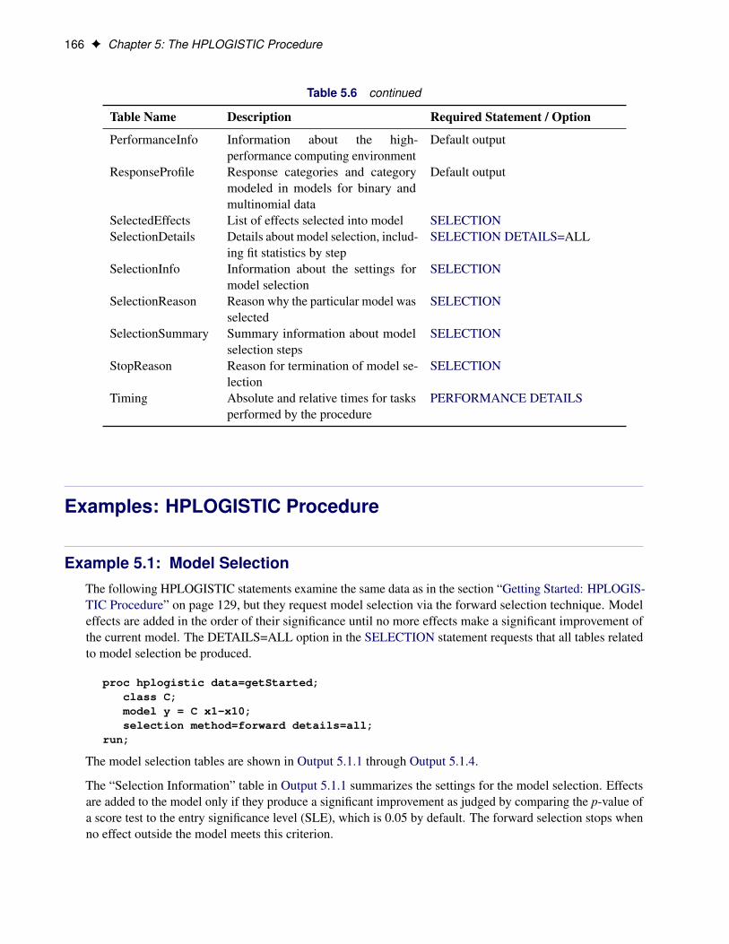
166 F Chapter 5: The HPLOGISTIC Procedure
Table 5.6 continued
Table Name Description Required Statement / Option
PerformanceInfo Information about the high-performance computing environment
Default output
ResponseProfile Response categories and categorymodeled in models for binary andmultinomial data
Default output
SelectedEffects List of effects selected into model SELECTIONSelectionDetails Details about model selection, includ-
ing fit statistics by stepSELECTION DETAILS=ALL
SelectionInfo Information about the settings formodel selection
SELECTION
SelectionReason Reason why the particular model wasselected
SELECTION
SelectionSummary Summary information about modelselection steps
SELECTION
StopReason Reason for termination of model se-lection
SELECTION
Timing Absolute and relative times for tasksperformed by the procedure
PERFORMANCE DETAILS
Examples: HPLOGISTIC Procedure
Example 5.1: Model SelectionThe following HPLOGISTIC statements examine the same data as in the section “Getting Started: HPLOGIS-TIC Procedure” on page 129, but they request model selection via the forward selection technique. Modeleffects are added in the order of their significance until no more effects make a significant improvement ofthe current model. The DETAILS=ALL option in the SELECTION statement requests that all tables relatedto model selection be produced.
proc hplogistic data=getStarted;class C;model y = C x1-x10;selection method=forward details=all;
run;
The model selection tables are shown in Output 5.1.1 through Output 5.1.4.
The “Selection Information” table in Output 5.1.1 summarizes the settings for the model selection. Effectsare added to the model only if they produce a significant improvement as judged by comparing the p-value ofa score test to the entry significance level (SLE), which is 0.05 by default. The forward selection stops whenno effect outside the model meets this criterion.
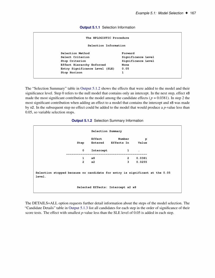
Example 5.1: Model Selection F 167
Output 5.1.1 Selection Information
The HPLOGISTIC Procedure
Selection Information
Selection Method ForwardSelect Criterion Significance LevelStop Criterion Significance LevelEffect Hierarchy Enforced NoneEntry Significance Level (SLE) 0.05Stop Horizon 1
The “Selection Summary” table in Output 5.1.2 shows the effects that were added to the model and theirsignificance level. Step 0 refers to the null model that contains only an intercept. In the next step, effect x8made the most significant contribution to the model among the candidate effects (p = 0.0381). In step 2 themost significant contribution when adding an effect to a model that contains the intercept and x8 was madeby x2. In the subsequent step no effect could be added to the model that would produce a p-value less than0.05, so variable selection stops.
Output 5.1.2 Selection Summary Information
Selection Summary
Effect Number pStep Entered Effects In Value
0 Intercept 1 .---------------------------------------------
1 x8 2 0.03812 x2 3 0.0255
Selection stopped because no candidate for entry is significant at the 0.05level.
Selected Effects: Intercept x2 x8
The DETAILS=ALL option requests further detail information about the steps of the model selection. The“Candidate Details” table in Output 5.1.3 list all candidates for each step in the order of significance of theirscore tests. The effect with smallest p-value less than the SLE level of 0.05 is added in each step.
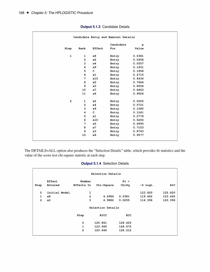
168 F Chapter 5: The HPLOGISTIC Procedure
Output 5.1.3 Candidate Details
Candidate Entry and Removal Details
Candidate pStep Rank Effect For Value
1 1 x8 Entry 0.03812 x2 Entry 0.04583 x4 Entry 0.05574 x9 Entry 0.16315 C Entry 0.18586 x1 Entry 0.27157 x10 Entry 0.44348 x5 Entry 0.76669 x3 Entry 0.8006
10 x7 Entry 0.866311 x6 Entry 0.9626
2 1 x2 Entry 0.02552 x4 Entry 0.07213 x9 Entry 0.10804 C Entry 0.12415 x1 Entry 0.27786 x10 Entry 0.52507 x5 Entry 0.69938 x7 Entry 0.71039 x3 Entry 0.8743
10 x6 Entry 0.9577
The DETAILS=ALL option also produces the “Selection Details” table, which provides fit statistics and thevalue of the score test chi-square statistic at each step.
Output 5.1.4 Selection Details
Selection Details
Effect Number Pr >Step Entered Effects In Chi-Square ChiSq -2 LogL AIC
0 Initial Model 1 123.820 125.8201 x8 2 4.2986 0.0381 119.462 123.4622 x2 3 4.9882 0.0255 114.396 120.396
Selection Details
Step AICC BIC
0 125.861 128.4251 123.586 128.6722 120.646 128.212
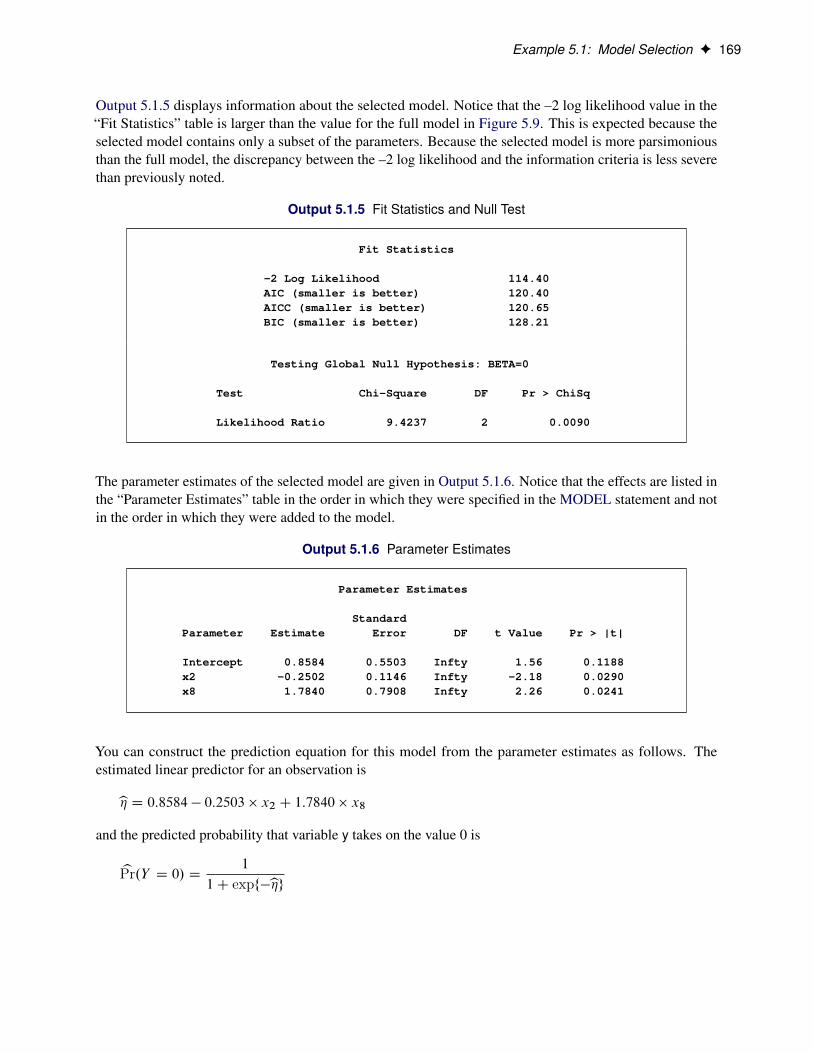
Example 5.1: Model Selection F 169
Output 5.1.5 displays information about the selected model. Notice that the –2 log likelihood value in the“Fit Statistics” table is larger than the value for the full model in Figure 5.9. This is expected because theselected model contains only a subset of the parameters. Because the selected model is more parsimoniousthan the full model, the discrepancy between the –2 log likelihood and the information criteria is less severethan previously noted.
Output 5.1.5 Fit Statistics and Null Test
Fit Statistics
-2 Log Likelihood 114.40AIC (smaller is better) 120.40AICC (smaller is better) 120.65BIC (smaller is better) 128.21
Testing Global Null Hypothesis: BETA=0
Test Chi-Square DF Pr > ChiSq
Likelihood Ratio 9.4237 2 0.0090
The parameter estimates of the selected model are given in Output 5.1.6. Notice that the effects are listed inthe “Parameter Estimates” table in the order in which they were specified in the MODEL statement and notin the order in which they were added to the model.
Output 5.1.6 Parameter Estimates
Parameter Estimates
StandardParameter Estimate Error DF t Value Pr > |t|
Intercept 0.8584 0.5503 Infty 1.56 0.1188x2 -0.2502 0.1146 Infty -2.18 0.0290x8 1.7840 0.7908 Infty 2.26 0.0241
You can construct the prediction equation for this model from the parameter estimates as follows. Theestimated linear predictor for an observation is
b� D 0:8584 � 0:2503 � x2 C 1:7840 � x8and the predicted probability that variable y takes on the value 0 is
bPr.Y D 0/ D1
1C expf�b�g
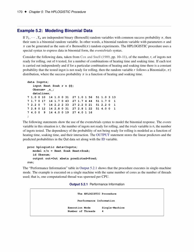
170 F Chapter 5: The HPLOGISTIC Procedure
Example 5.2: Modeling Binomial DataIf Y1; � � � ; Yn are independent binary (Bernoulli) random variables with common success probability � , thentheir sum is a binomial random variable. In other words, a binomial random variable with parameters n and� can be generated as the sum of n Bernoulli(�) random experiments. The HPLOGISTIC procedure uses aspecial syntax to express data in binomial form, the events/trials syntax.
Consider the following data, taken from Cox and Snell (1989, pp. 10–11), of the number, r, of ingots notready for rolling, out of n tested, for a number of combinations of heating time and soaking time. If each testis carried out independently and if for a particular combination of heating and soaking time there is a constantprobability that the tested ingot is not ready for rolling, then the random variable r follows a Binomial.n; �/distribution, where the success probability � is a function of heating and soaking time.
data Ingots;input Heat Soak r n @@;Obsnum= _n_;datalines;
7 1.0 0 10 14 1.0 0 31 27 1.0 1 56 51 1.0 3 137 1.7 0 17 14 1.7 0 43 27 1.7 4 44 51 1.7 0 17 2.2 0 7 14 2.2 2 33 27 2.2 0 21 51 2.2 0 17 2.8 0 12 14 2.8 0 31 27 2.8 1 22 51 4.0 0 17 4.0 0 9 14 4.0 0 19 27 4.0 1 16;
The following statements show the use of the events/trials syntax to model the binomial response. The eventsvariable in this situation is r, the number of ingots not ready for rolling, and the trials variable is n, the numberof ingots tested. The dependency of the probability of not being ready for rolling is modeled as a function ofheating time, soaking time, and their interaction. The OUTPUT statement stores the linear predictors and thepredicted probabilities in the Out data set along with the ID variable.
proc hplogistic data=Ingots;model r/n = Heat Soak Heat*Soak;id Obsnum;output out=Out xbeta predicted=Pred;
run;
The “Performance Information” table in Output 5.2.1 shows that the procedure executes in single-machinemode. The example is executed on a single machine with the same number of cores as the number of threadsused; that is, one computational thread was spawned per CPU.
Output 5.2.1 Performance Information
The HPLOGISTIC Procedure
Performance Information
Execution Mode Single-MachineNumber of Threads 4

Example 5.2: Modeling Binomial Data F 171
The “Model Information” table shows that the data are modeled as binomially distributed with a logit linkfunction (Output 5.2.2). This is the default link function in the HPLOGISTIC procedure for binary andbinomial data. The procedure estimates the parameters of the model by a Newton-Raphson algorithm.
Output 5.2.2 Model Information and Number of Observations
Model Information
Data Source WORK.INGOTSResponse Variable (Events) rResponse Variable (Trials) nDistribution BinomialLink Function LogitOptimization Technique Newton-Raphson with Ridging
Number of Observations Read 19Number of Observations Used 19Number of Events 12Number of Trials 387
The second table in Output 5.2.2 shows that all 19 observations in the data set were used in the analysis, andthat the total number of events and trials equal 12 and 387, respectively. These are the sums of the variables rand n across all observations.
Output 5.2.3 displays the “Iteration History” and convergence status tables for this run. The HPLOGISTICprocedure converged after four iterations (not counting the initial setup iteration) and meets the GCONV=convergence criterion.
Output 5.2.3 Iteration History and Convergence Status
Iteration History
Objective MaxIteration Evaluations Function Change Gradient
0 4 0.7676329445 . 6.3780021 2 0.7365832479 0.03104970 0.7549022 2 0.7357086248 0.00087462 0.0236233 2 0.7357075299 0.00000109 0.000034 2 0.7357075299 0.00000000 5.42E-11
Convergence criterion (GCONV=1E-8) satisfied.
Output 5.2.4 displays the “Dimensions” table for the model. There are four columns in the design matrix ofthe model (the X matrix); they correspond to the intercept, the Heat effect, the Soak effect, and the interactionof the Heat and Soak effects. The model is nonsingular, since the rank of the crossproducts matrix equals thenumber of columns in X. All parameters are estimable and participate in the optimization.
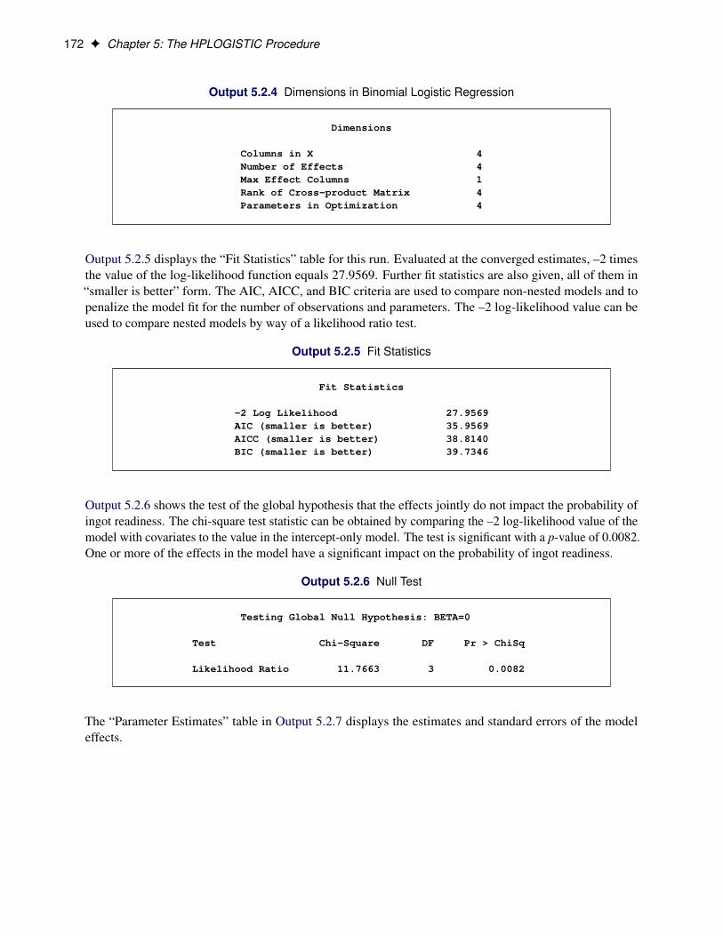
172 F Chapter 5: The HPLOGISTIC Procedure
Output 5.2.4 Dimensions in Binomial Logistic Regression
Dimensions
Columns in X 4Number of Effects 4Max Effect Columns 1Rank of Cross-product Matrix 4Parameters in Optimization 4
Output 5.2.5 displays the “Fit Statistics” table for this run. Evaluated at the converged estimates, –2 timesthe value of the log-likelihood function equals 27.9569. Further fit statistics are also given, all of them in“smaller is better” form. The AIC, AICC, and BIC criteria are used to compare non-nested models and topenalize the model fit for the number of observations and parameters. The –2 log-likelihood value can beused to compare nested models by way of a likelihood ratio test.
Output 5.2.5 Fit Statistics
Fit Statistics
-2 Log Likelihood 27.9569AIC (smaller is better) 35.9569AICC (smaller is better) 38.8140BIC (smaller is better) 39.7346
Output 5.2.6 shows the test of the global hypothesis that the effects jointly do not impact the probability ofingot readiness. The chi-square test statistic can be obtained by comparing the –2 log-likelihood value of themodel with covariates to the value in the intercept-only model. The test is significant with a p-value of 0.0082.One or more of the effects in the model have a significant impact on the probability of ingot readiness.
Output 5.2.6 Null Test
Testing Global Null Hypothesis: BETA=0
Test Chi-Square DF Pr > ChiSq
Likelihood Ratio 11.7663 3 0.0082
The “Parameter Estimates” table in Output 5.2.7 displays the estimates and standard errors of the modeleffects.
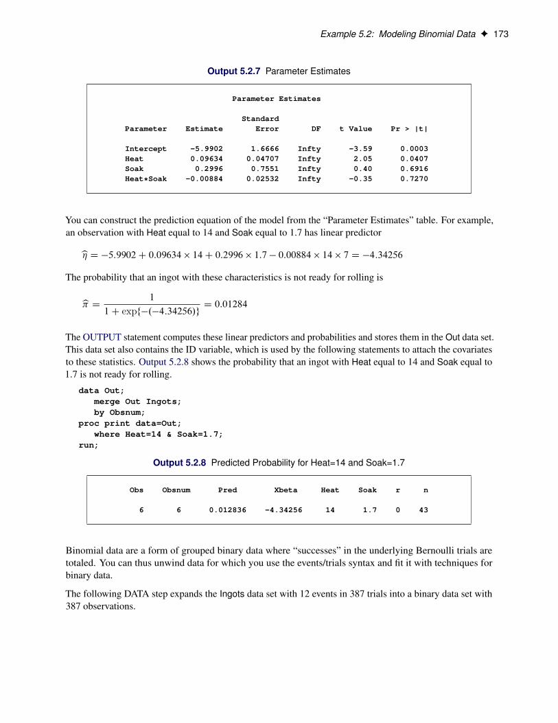
Example 5.2: Modeling Binomial Data F 173
Output 5.2.7 Parameter Estimates
Parameter Estimates
StandardParameter Estimate Error DF t Value Pr > |t|
Intercept -5.9902 1.6666 Infty -3.59 0.0003Heat 0.09634 0.04707 Infty 2.05 0.0407Soak 0.2996 0.7551 Infty 0.40 0.6916Heat*Soak -0.00884 0.02532 Infty -0.35 0.7270
You can construct the prediction equation of the model from the “Parameter Estimates” table. For example,an observation with Heat equal to 14 and Soak equal to 1.7 has linear predictor
b� D �5:9902C 0:09634 � 14C 0:2996 � 1:7 � 0:00884 � 14 � 7 D �4:34256The probability that an ingot with these characteristics is not ready for rolling is
b� D 1
1C expf�.�4:34256/gD 0:01284
The OUTPUT statement computes these linear predictors and probabilities and stores them in the Out data set.This data set also contains the ID variable, which is used by the following statements to attach the covariatesto these statistics. Output 5.2.8 shows the probability that an ingot with Heat equal to 14 and Soak equal to1.7 is not ready for rolling.
data Out;merge Out Ingots;by Obsnum;
proc print data=Out;where Heat=14 & Soak=1.7;
run;
Output 5.2.8 Predicted Probability for Heat=14 and Soak=1.7
Obs Obsnum Pred Xbeta Heat Soak r n
6 6 0.012836 -4.34256 14 1.7 0 43
Binomial data are a form of grouped binary data where “successes” in the underlying Bernoulli trials aretotaled. You can thus unwind data for which you use the events/trials syntax and fit it with techniques forbinary data.
The following DATA step expands the Ingots data set with 12 events in 387 trials into a binary data set with387 observations.

174 F Chapter 5: The HPLOGISTIC Procedure
data Ingots_binary;set Ingots;do i=1 to n;
if i <= r then y=1; else y = 0;output;
end;run;
The following HPLOGISTIC statements fit the model with Heat effect, Soak effect, and their interactionto the binary data set. The event=’1’ response-variable option in the MODEL statement ensures that theHPLOGISTIC procedure models the probability that the variable y takes on the value (‘1’).
proc hplogistic data=Ingots_binary;model y(event='1') = Heat Soak Heat*Soak;
run;
Output 5.2.9 displays the “Performance Information”, “Model Information,” “Number of Observations,” andthe “Response Profile” tables. The data are now modeled as binary (Bernoulli distributed) with a logit linkfunction. The “Response Profile” table shows that the binary response breaks down into 375 observationswhere y equals zero and 12 observations where y equals 1.
Output 5.2.9 Model Information in Binary Model
The HPLOGISTIC Procedure
Performance Information
Execution Mode Single-MachineNumber of Threads 4
Model Information
Data Source WORK.INGOTS_BINARYResponse Variable yDistribution BinaryLink Function LogitOptimization Technique Newton-Raphson with Ridging
Number of Observations Read 387Number of Observations Used 387
Response Profile
Ordered TotalValue y Frequency
1 0 3752 1 12
You are modeling the probability that y='1'.
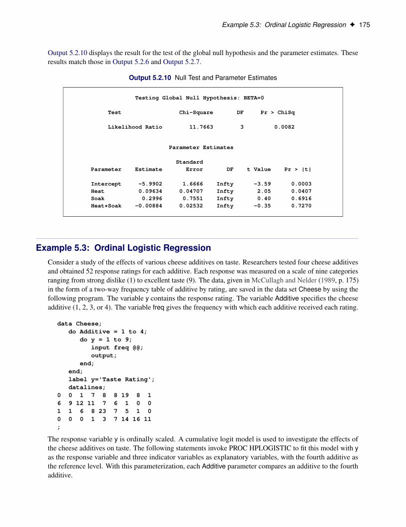
Example 5.3: Ordinal Logistic Regression F 175
Output 5.2.10 displays the result for the test of the global null hypothesis and the parameter estimates. Theseresults match those in Output 5.2.6 and Output 5.2.7.
Output 5.2.10 Null Test and Parameter Estimates
Testing Global Null Hypothesis: BETA=0
Test Chi-Square DF Pr > ChiSq
Likelihood Ratio 11.7663 3 0.0082
Parameter Estimates
StandardParameter Estimate Error DF t Value Pr > |t|
Intercept -5.9902 1.6666 Infty -3.59 0.0003Heat 0.09634 0.04707 Infty 2.05 0.0407Soak 0.2996 0.7551 Infty 0.40 0.6916Heat*Soak -0.00884 0.02532 Infty -0.35 0.7270
Example 5.3: Ordinal Logistic RegressionConsider a study of the effects of various cheese additives on taste. Researchers tested four cheese additivesand obtained 52 response ratings for each additive. Each response was measured on a scale of nine categoriesranging from strong dislike (1) to excellent taste (9). The data, given in McCullagh and Nelder (1989, p. 175)in the form of a two-way frequency table of additive by rating, are saved in the data set Cheese by using thefollowing program. The variable y contains the response rating. The variable Additive specifies the cheeseadditive (1, 2, 3, or 4). The variable freq gives the frequency with which each additive received each rating.
data Cheese;do Additive = 1 to 4;
do y = 1 to 9;input freq @@;output;
end;end;label y='Taste Rating';datalines;
0 0 1 7 8 8 19 8 16 9 12 11 7 6 1 0 01 1 6 8 23 7 5 1 00 0 0 1 3 7 14 16 11;
The response variable y is ordinally scaled. A cumulative logit model is used to investigate the effects ofthe cheese additives on taste. The following statements invoke PROC HPLOGISTIC to fit this model with yas the response variable and three indicator variables as explanatory variables, with the fourth additive asthe reference level. With this parameterization, each Additive parameter compares an additive to the fourthadditive.
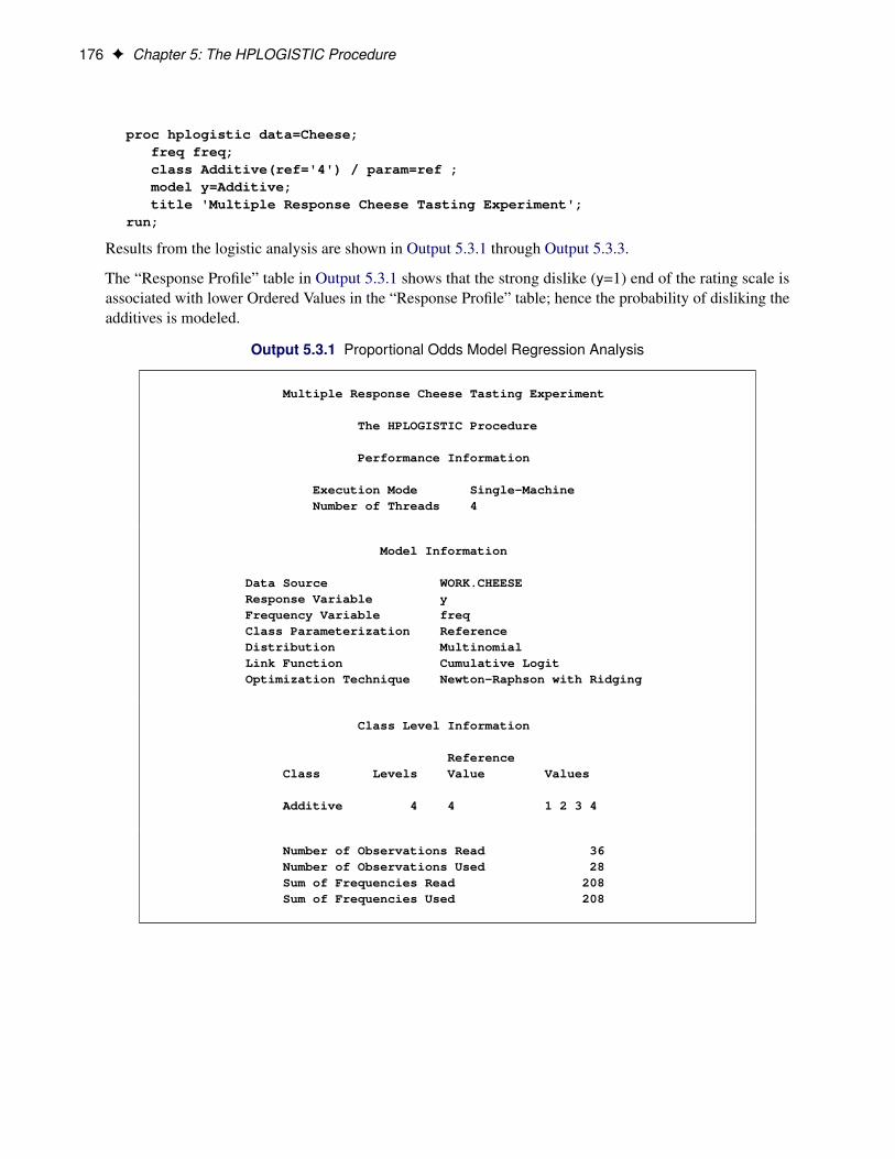
176 F Chapter 5: The HPLOGISTIC Procedure
proc hplogistic data=Cheese;freq freq;class Additive(ref='4') / param=ref ;model y=Additive;title 'Multiple Response Cheese Tasting Experiment';
run;
Results from the logistic analysis are shown in Output 5.3.1 through Output 5.3.3.
The “Response Profile” table in Output 5.3.1 shows that the strong dislike (y=1) end of the rating scale isassociated with lower Ordered Values in the “Response Profile” table; hence the probability of disliking theadditives is modeled.
Output 5.3.1 Proportional Odds Model Regression Analysis
Multiple Response Cheese Tasting Experiment
The HPLOGISTIC Procedure
Performance Information
Execution Mode Single-MachineNumber of Threads 4
Model Information
Data Source WORK.CHEESEResponse Variable yFrequency Variable freqClass Parameterization ReferenceDistribution MultinomialLink Function Cumulative LogitOptimization Technique Newton-Raphson with Ridging
Class Level Information
ReferenceClass Levels Value Values
Additive 4 4 1 2 3 4
Number of Observations Read 36Number of Observations Used 28Sum of Frequencies Read 208Sum of Frequencies Used 208

Example 5.3: Ordinal Logistic Regression F 177
Output 5.3.1 continued
Response Profile
Ordered Taste TotalValue Rating Frequency
1 1 72 2 103 3 194 4 275 5 416 6 287 7 398 8 259 9 12
You are modeling the probabilities of levels of y having lower Ordered Valuesin the Response Profile Table.
Output 5.3.2 Proportional Odds Model Regression Analysis
Iteration History
Objective MaxIteration Evaluations Function Change Gradient
0 4 2.0668312595 . 0.1374121 2 1.7319560317 0.33487523 0.0627572 2 1.7105150048 0.02144103 0.0089193 2 1.7099716191 0.00054339 0.000354 2 1.7099709251 0.00000069 6.981E-75 2 1.7099709251 0.00000000 2.98E-12
Convergence criterion (GCONV=1E-8) satisfied.
Dimensions
Columns in X 11Number of Effects 2Max Effect Columns 3Rank of Cross-product Matrix 11Parameters in Optimization 11
Fit Statistics
-2 Log Likelihood 711.35AIC (smaller is better) 733.35AICC (smaller is better) 734.69BIC (smaller is better) 770.06

178 F Chapter 5: The HPLOGISTIC Procedure
Output 5.3.2 continued
Testing Global Null Hypothesis: BETA=0
Test Chi-Square DF Pr > ChiSq
Likelihood Ratio 148.4539 3 <.0001
The positive value (1.6128) for the parameter estimate for Additive=1 in Output 5.3.3 indicates a tendencytoward the lower-numbered categories of the first cheese additive relative to the fourth. In other words, thefourth additive tastes better than the first additive. Similarly, the second and third additives are both lessfavorable than the fourth additive. The relative magnitudes of these slope estimates imply the preferenceordering: fourth, first, third, second.
Output 5.3.3 Proportional Odds Model Regression Analysis
Parameter Estimates
Taste StandardParameter Rating Estimate Error DF t Value Pr > |t|
Intercept 1 -7.0802 0.5640 Infty -12.55 <.0001Intercept 2 -6.0250 0.4764 Infty -12.65 <.0001Intercept 3 -4.9254 0.4257 Infty -11.57 <.0001Intercept 4 -3.8568 0.3880 Infty -9.94 <.0001Intercept 5 -2.5206 0.3453 Infty -7.30 <.0001Intercept 6 -1.5685 0.3122 Infty -5.02 <.0001Intercept 7 -0.06688 0.2738 Infty -0.24 0.8071Intercept 8 1.4930 0.3357 Infty 4.45 <.0001Additive 1 1.6128 0.3805 Infty 4.24 <.0001Additive 2 4.9646 0.4767 Infty 10.41 <.0001Additive 3 3.3227 0.4218 Infty 7.88 <.0001
Example 5.4: Conditional Logistic Regression for Matched Pairs DataIn matched pairs (case-control) studies, conditional logistic regression is used to investigate the relationshipbetween an outcome of being an event (case) or a non-event (control) and a set of prognostic factors.
The following data are a subset of the data from the Los Angeles Study of the Endometrial Cancer Datain Breslow and Day (1980). There are 63 matched pairs, each consisting of a case of endometrial cancer(Outcome=1) and a control (Outcome=0). The case and corresponding control have the same ID. Twoprognostic factors are included: Gall (an indicator variable for gall bladder disease) and Hyper (an indicatorvariable for hypertension). The goal of the case-control analysis is to determine the relative risk for gallbladder disease, controlling for the effect of hypertension.
data Data1;do ID=1 to 63;
do Outcome = 1 to 0 by -1;input Gall Hyper @@;
Example 5.4: Conditional Logistic Regression for Matched Pairs Data F 179
output;end;
end;datalines;
0 0 0 0 0 0 0 0 0 1 0 1 0 0 1 0 1 0 0 10 1 0 0 1 0 0 0 1 1 0 1 0 0 0 0 0 0 0 01 0 0 0 0 0 0 1 1 0 0 1 1 0 1 0 1 0 0 10 1 0 0 0 0 1 1 0 0 1 1 0 0 0 1 0 1 0 00 0 1 1 0 1 0 1 0 1 0 0 0 0 0 0 0 0 0 00 0 0 1 1 0 0 1 0 0 0 1 1 0 0 0 0 1 0 00 1 0 0 0 1 0 0 0 1 0 0 0 0 0 0 1 1 1 10 0 0 1 0 1 0 0 0 1 0 1 0 1 0 1 0 1 0 00 0 0 0 0 1 1 0 0 0 0 1 0 0 0 0 1 0 0 00 0 0 0 1 1 0 0 0 1 0 0 0 0 0 0 0 1 0 10 0 0 0 0 1 0 1 0 1 0 0 0 1 0 0 1 0 0 00 0 0 0 1 1 1 0 0 0 0 0 0 0 0 0 1 1 0 01 0 1 0 0 1 0 0 1 0 0 0;
When each matched set consists of one event and one non-event, the conditional likelihood is given byYi
.1C exp.�.xi1 � xi0/0 /�1
where xi1 and xi0 are vectors that represent the prognostic factors for the event and non-event, respectively,of the i th matched set. This likelihood is identical to the likelihood of fitting a logistic regression model to aset of data with constant response, where the model contains no intercept term and has explanatory variablesgiven by di D xi1 � xi0 (Breslow 1982).
To apply this method, the following DATA step transforms each matched pair into a single observation,where the variables Gall and Hyper contain the differences between the corresponding values for the case andthe control (case – control). The variable Outcome, which is used as the response variable in the logisticregression model, is given a constant value of 0 (which is the Outcome value for the control, although anyconstant, numeric or character, suffices).
data Data2;set Data1;drop id1 gall1 hyper1;retain id1 gall1 hyper1 0;if (ID = id1) then do;
Gall=gall1-Gall; Hyper=hyper1-Hyper;output;
end;else do;
id1=ID; gall1=Gall; hyper1=Hyper;end;
run;
Note that there are 63 observations in the data set, one for each matched pair. Since the number of observations(n) is halved, statistics that depend on n such as R2 will be incorrect. The variable Outcome has a constantvalue of 0.
In the following statements, PROC HPLOGISTIC is invoked with the NOINT option to obtain the conditionallogistic model estimates. Because the option CL is specified, PROC HPLOGISTIC computes a 95%confidence interval for the parameter.
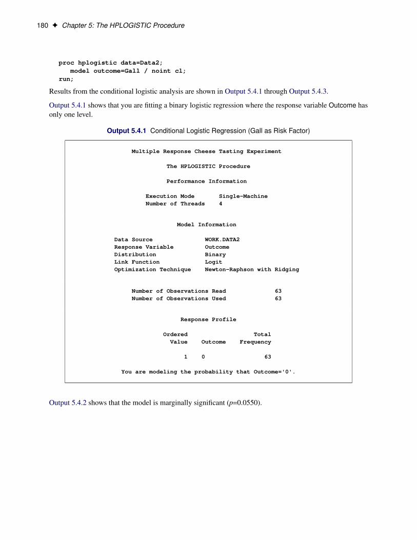
180 F Chapter 5: The HPLOGISTIC Procedure
proc hplogistic data=Data2;model outcome=Gall / noint cl;
run;
Results from the conditional logistic analysis are shown in Output 5.4.1 through Output 5.4.3.
Output 5.4.1 shows that you are fitting a binary logistic regression where the response variable Outcome hasonly one level.
Output 5.4.1 Conditional Logistic Regression (Gall as Risk Factor)
Multiple Response Cheese Tasting Experiment
The HPLOGISTIC Procedure
Performance Information
Execution Mode Single-MachineNumber of Threads 4
Model Information
Data Source WORK.DATA2Response Variable OutcomeDistribution BinaryLink Function LogitOptimization Technique Newton-Raphson with Ridging
Number of Observations Read 63Number of Observations Used 63
Response Profile
Ordered TotalValue Outcome Frequency
1 0 63
You are modeling the probability that Outcome='0'.
Output 5.4.2 shows that the model is marginally significant (p=0.0550).
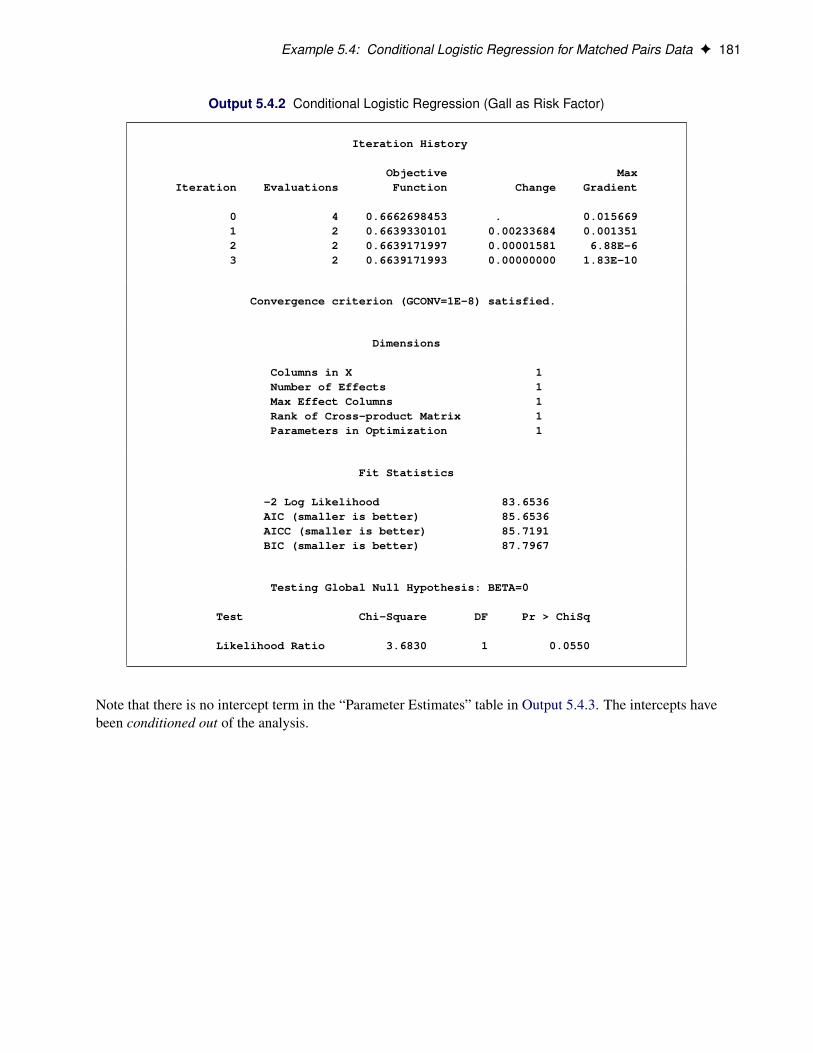
Example 5.4: Conditional Logistic Regression for Matched Pairs Data F 181
Output 5.4.2 Conditional Logistic Regression (Gall as Risk Factor)
Iteration History
Objective MaxIteration Evaluations Function Change Gradient
0 4 0.6662698453 . 0.0156691 2 0.6639330101 0.00233684 0.0013512 2 0.6639171997 0.00001581 6.88E-63 2 0.6639171993 0.00000000 1.83E-10
Convergence criterion (GCONV=1E-8) satisfied.
Dimensions
Columns in X 1Number of Effects 1Max Effect Columns 1Rank of Cross-product Matrix 1Parameters in Optimization 1
Fit Statistics
-2 Log Likelihood 83.6536AIC (smaller is better) 85.6536AICC (smaller is better) 85.7191BIC (smaller is better) 87.7967
Testing Global Null Hypothesis: BETA=0
Test Chi-Square DF Pr > ChiSq
Likelihood Ratio 3.6830 1 0.0550
Note that there is no intercept term in the “Parameter Estimates” table in Output 5.4.3. The intercepts havebeen conditioned out of the analysis.
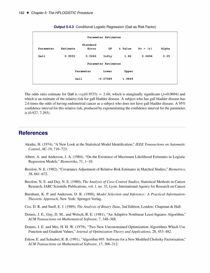
182 F Chapter 5: The HPLOGISTIC Procedure
Output 5.4.3 Conditional Logistic Regression (Gall as Risk Factor)
Parameter Estimates
StandardParameter Estimate Error DF t Value Pr > |t| Alpha
Gall 0.9555 0.5262 Infty 1.82 0.0694 0.05
Parameter Estimates
Parameter Lower Upper
Gall -0.07589 1.9869
The odds ratio estimate for Gall is exp.0:9555/ D 2:60, which is marginally significant (p=0.0694) andwhich is an estimate of the relative risk for gall bladder disease. A subject who has gall bladder disease has2.6 times the odds of having endometrial cancer as a subject who does not have gall bladder disease. A 95%confidence interval for this relative risk, produced by exponentiating the confidence interval for the parameter,is (0.927, 7.293).
References
Akaike, H. (1974), “A New Look at the Statistical Model Identification,” IEEE Transactions on AutomaticControl, AC-19, 716–723.
Albert, A. and Anderson, J. A. (1984), “On the Existence of Maximum Likelihood Estimates in LogisticRegression Models,” Biometrika, 71, 1–10.
Breslow, N. E. (1982), “Covariance Adjustment of Relative-Risk Estimates in Matched Studies,” Biometrics,38, 661–672.
Breslow, N. E. and Day, N. E. (1980), The Analysis of Case-Control Studies, Statistical Methods in CancerResearch, IARC Scientific Publications, vol. 1, no. 32, Lyon: International Agency for Research on Cancer.
Burnham, K. P. and Anderson, D. R. (1998), Model Selection and Inference: A Practical Information-Theoretic Approach, New York: Springer-Verlag.
Cox, D. R. and Snell, E. J. (1989), The Analysis of Binary Data, 2nd Edition, London: Chapman & Hall.
Dennis, J. E., Gay, D. M., and Welsch, R. E. (1981), “An Adaptive Nonlinear Least-Squares Algorithm,”ACM Transactions on Mathematical Software, 7, 348–368.
Dennis, J. E. and Mei, H. H. W. (1979), “Two New Unconstrained Optimization Algorithms Which UseFunction and Gradient Values,” Journal of Optimization Theory and Applications, 28, 453–482.
Eskow, E. and Schnabel, R. B. (1991), “Algorithm 695: Software for a New Modified Cholesky Factorization,”ACM Transactions on Mathematical Software, 17, 306–312.

References F 183
Fletcher, R. (1987), Practical Methods of Optimization, 2nd Edition, Chichester, UK: John Wiley & Sons.
Gay, D. M. (1983), “Subroutines for Unconstrained Minimization,” ACM Transactions on MathematicalSoftware, 9, 503–524.
Hosmer, D. W., Jr. and Lemeshow, S. (2000), Applied Logistic Regression, 2nd Edition, New York: JohnWiley & Sons.
Hurvich, C. M. and Tsai, C.-L. (1989), “Regression and Time Series Model Selection in Small Samples,”Biometrika, 76, 297–307.
Magee, L. (1990), “R2 Measures Based on Wald and Likelihood Ratio Joint Significant Tests,” AmericanStatistician, 44, 250–253.
McCullagh, P. and Nelder, J. A. (1989), Generalized Linear Models, 2nd Edition, London: Chapman & Hall.
Moré, J. J. and Sorensen, D. C. (1983), “Computing a Trust-Region Step,” SIAM Journal on Scientific andStatistical Computing, 4, 553–572.
Nagelkerke, N. J. D. (1991), “A Note on a General Definition of the Coefficient of Determination,” Biometrika,78, 691–692.
Santner, T. J. and Duffy, D. E. (1986), “A Note on A. Albert and J. A. Anderson’s Conditions for the Existenceof Maximum Likelihood Estimates in Logistic Regression Models,” Biometrika, 73, 755–758.
Schwarz, G. (1978), “Estimating the Dimension of a Model,” Annals of Statistics, 6, 461–464.

184

Chapter 6
The HPLMIXED Procedure
ContentsOverview: HPLMIXED Procedure . . . . . . . . . . . . . . . . . . . . . . . . . . . . . . . 186
PROC HPLMIXED Features . . . . . . . . . . . . . . . . . . . . . . . . . . . . . . 187Notation for the Mixed Model . . . . . . . . . . . . . . . . . . . . . . . . . . . . . . 188PROC HPLMIXED Contrasted with Other SAS Procedures . . . . . . . . . . . . . . 189
Getting Started: HPLMIXED Procedure . . . . . . . . . . . . . . . . . . . . . . . . . . . . 189Mixed Model Analysis of Covariance with Many Groups . . . . . . . . . . . . . . . 189
Syntax: HPLMIXED Procedure . . . . . . . . . . . . . . . . . . . . . . . . . . . . . . . . 192PROC HPLMIXED Statement . . . . . . . . . . . . . . . . . . . . . . . . . . . . . . 193CLASS Statement . . . . . . . . . . . . . . . . . . . . . . . . . . . . . . . . . . . . 198MODEL Statement . . . . . . . . . . . . . . . . . . . . . . . . . . . . . . . . . . . . 198PARMS Statement . . . . . . . . . . . . . . . . . . . . . . . . . . . . . . . . . . . . 199PERFORMANCE Statement . . . . . . . . . . . . . . . . . . . . . . . . . . . . . . 201RANDOM Statement . . . . . . . . . . . . . . . . . . . . . . . . . . . . . . . . . . 201REPEATED Statement . . . . . . . . . . . . . . . . . . . . . . . . . . . . . . . . . . 208
Details: HPLMIXED Procedure . . . . . . . . . . . . . . . . . . . . . . . . . . . . . . . . 209Linear Mixed Models Theory . . . . . . . . . . . . . . . . . . . . . . . . . . . . . . 209
Matrix Notation . . . . . . . . . . . . . . . . . . . . . . . . . . . . . . . . . 209Formulation of the Mixed Model . . . . . . . . . . . . . . . . . . . . . . . . 210Estimating Covariance Parameters in the Mixed Model . . . . . . . . . . . . 214Estimating Fixed and Random Effects in the Mixed Model . . . . . . . . . . 215Statistical Properties . . . . . . . . . . . . . . . . . . . . . . . . . . . . . . 216
Computational Method . . . . . . . . . . . . . . . . . . . . . . . . . . . . . . . . . . 217Distributed Computing . . . . . . . . . . . . . . . . . . . . . . . . . . . . . 217Multithreading . . . . . . . . . . . . . . . . . . . . . . . . . . . . . . . . . 217
Displayed Output . . . . . . . . . . . . . . . . . . . . . . . . . . . . . . . . . . . . . 218Performance Information . . . . . . . . . . . . . . . . . . . . . . . . . . . . 218Model Information . . . . . . . . . . . . . . . . . . . . . . . . . . . . . . . 218Class Level Information . . . . . . . . . . . . . . . . . . . . . . . . . . . . 218Dimensions . . . . . . . . . . . . . . . . . . . . . . . . . . . . . . . . . . . 218Number of Observations . . . . . . . . . . . . . . . . . . . . . . . . . . . . 218Optimization Information . . . . . . . . . . . . . . . . . . . . . . . . . . . . 219Iteration History . . . . . . . . . . . . . . . . . . . . . . . . . . . . . . . . 219Convergence Status . . . . . . . . . . . . . . . . . . . . . . . . . . . . . . . 220Covariance Parameter Estimates . . . . . . . . . . . . . . . . . . . . . . . . 220Fit Statistics . . . . . . . . . . . . . . . . . . . . . . . . . . . . . . . . . . . 220Timing Information . . . . . . . . . . . . . . . . . . . . . . . . . . . . . . . 221
186 F Chapter 6: The HPLMIXED Procedure
ODS Table Names . . . . . . . . . . . . . . . . . . . . . . . . . . . . . . . . . . . . 221Examples: HPLMIXED Procedure . . . . . . . . . . . . . . . . . . . . . . . . . . . . . . . 221
Example 6.1: Computing BLUPs for a Large Number of Subjects . . . . . . . . . . . 221References . . . . . . . . . . . . . . . . . . . . . . . . . . . . . . . . . . . . . . . . . . . 224
Overview: HPLMIXED ProcedureThe HPLMIXED procedure fits a variety of mixed linear models to data and enables you to use these fittedmodels to make statistical inferences about the data. A mixed linear model is a generalization of the standardlinear model used in the GLM procedure in SAS/STAT software; the generalization is that the data arepermitted to exhibit correlation and nonconstant variability. Therefore, the mixed linear model provides youwith the flexibility of modeling not only the means of your data (as in the standard linear model) but alsotheir variances and covariances.
The primary assumptions underlying the analyses performed by PROC HPLMIXED are as follows:
• The data are normally distributed (Gaussian).
• The means (expected values) of the data are linear in terms of a certain set of parameters.
• The variances and covariances of the data are in terms of a different set of parameters, and they exhibita structure that matches one of those available in PROC HPLMIXED.
Because Gaussian data can be modeled entirely in terms of their means and variances/covariances, the twosets of parameters in a mixed linear model actually specify the complete probability distribution of the data.The parameters of the mean model are referred to as fixed-effects parameters, and the parameters of thevariance-covariance model are referred to as covariance parameters.
The fixed-effects parameters are associated with known explanatory variables, as in the standard linear model.These variables can be either qualitative (as in the traditional analysis of variance) or quantitative (as instandard linear regression). However, the covariance parameters are what distinguishes the mixed linearmodel from the standard linear model.
The need for covariance parameters arises quite frequently in applications; the following scenarios are themost typical:
• The experimental units on which the data are measured can be grouped into clusters, and the data froma common cluster are correlated. This scenario can be generalized to include one set of clusters nestedwithin another. For example, if students are the experimental unit, they can be clustered into classes,which in turn can be clustered into schools. Each level of this hierarchy can introduce an additionalsource of variability and correlation.
• Repeated measurements are taken on the same experimental unit, and these repeated measurementsare correlated or exhibit variability that changes. This scenario occurs in longitudinal studies, whererepeated measurements are taken over time. Alternatively, the repeated measures could be spatial ormultivariate in nature.
PROC HPLMIXED Features F 187
PROC HPLMIXED provides a variety of covariance structures to handle these two scenarios. The mostcommon covariance structures arise from the use of random-effects parameters, which are additional unknownrandom variables that are assumed to affect the variability of the data. The variances of the random-effectsparameters, commonly known as variance components, become the covariance parameters for this particularstructure. Traditional mixed linear models contain both fixed- and random-effects parameters; in fact, it is thecombination of these two types of effects that led to the name mixed model. PROC HPLMIXED fits not onlythese traditional variance component models but also numerous other covariance structures.
PROC HPLMIXED fits the structure you select to the data by using the method of restricted maximumlikelihood (REML), also known as residual maximum likelihood. It is here that the Gaussian assumption forthe data is exploited.
PROC HPLMIXED runs in either single-machine mode or distributed mode.
NOTE: Distributed mode requires SAS High-Performance Statistics.
PROC HPLMIXED FeaturesPROC HPLMIXED provides easy accessibility to numerous mixed linear models that are useful in manycommon statistical analyses.
Here are some basic features of PROC HPLMIXED:
• covariance structures, including variance components, compound symmetry, unstructured, AR(1),Toeplitz, and factor analytic
• MODEL, RANDOM, and REPEATED statements for model specification as in the MIXED procedure
• appropriate standard errors, t tests, and F tests for all specified estimable linear combinations of fixedand random effects
• a subject effect that enables blocking
• REML and ML (maximum likelihood) estimation methods implemented with a variety of optimizationalgorithms
• capacity to handle unbalanced data
• special dense and sparse algorithms that take advantage of distributed and multicore computingenvironments
Because the HPLMIXED procedure is a high-performance analytical procedure, it also does the following:
• enables you to run in distributed mode on a cluster of machines that distribute the data and thecomputations
• enables you to run in single-machine mode on the server where SAS is installed
• exploits all the available cores and concurrent threads, regardless of execution mode

188 F Chapter 6: The HPLMIXED Procedure
For more information, see the section “Processing Modes” on page 6 in Chapter 2, “Shared Concepts andTopics.”
PROC HPLMIXED uses the Output Delivery System (ODS), a SAS subsystem that provides capabilities fordisplaying and controlling the output from SAS procedures. ODS enables you to convert any output fromPROC HPLMIXED into a SAS data set. See the section “ODS Table Names” on page 221.
Notation for the Mixed ModelThis section introduces the mathematical notation used throughout this chapter to describe the mixed linearmodel and assumes familiarity with basic matrix algebra (for an overview, see Searle 1982). A more detaileddescription of the mixed model is contained in the section “Linear Mixed Models Theory” on page 209.
A statistical model is a mathematical description of how data are generated. The standard linear model, asused by the GLM procedure, is one of the most common statistical models:
y D Xˇ C �
In this expression, y represents a vector of observed data, ˇ is an unknown vector of fixed-effects parameterswith a known design matrix X, and � is an unknown random error vector that models the statistical noisearound Xˇ. The focus of the standard linear model is to model the mean of y by using the fixed-effectsparameters ˇ. The residual errors � are assumed to be independent and identically distributed Gaussianrandom variables with mean 0 and variance �2.
The mixed model generalizes the standard linear model as follows:
y D Xˇ C Z C �
Here, is an unknown vector of random-effects parameters with a known design matrix Z, and � is anunknown random error vector whose elements are no longer required to be independent and homogeneous.
To further develop this notion of variance modeling, assume that and � are Gaussian random variables thatare uncorrelated, have expectations 0, and have variances G and R, respectively. The variance of y is thus
V D ZGZ0 CR
Note that when R D �2I and Z D 0, the mixed model reduces to the standard linear model.
You can model the variance of the data y by specifying the structure of Z, G, and R. The model matrix Z isset up in the same fashion as X, the model matrix for the fixed-effects parameters. For G and R, you mustselect some covariance structure. Possible covariance structures include the following:
• variance components
• compound symmetry (common covariance plus diagonal)
• unstructured (general covariance)
• autoregressive
• spatial
PROC HPLMIXED Contrasted with Other SAS Procedures F 189
• general linear
• factor analytic
By appropriately defining the model matrices X and Z in addition to the covariance structure matrices G andR, you can perform numerous mixed model analyses.
PROC HPLMIXED Contrasted with Other SAS ProceduresThe RANDOM and REPEATED statements of the HPLMIXED procedure follow the convention of the samestatements in the MIXED procedure in SAS/STAT software. For information about how these statementsdiffer from RANDOM and REPEATED statements in the MIXED procedure, see the documentation for theMIXED procedure in the SAS/STAT User’s Guide.
The GLIMMIX procedure in SAS/STAT software fits generalized linear mixed models. Linear mixedmodels—where the data are normally distributed, given the random effects—are in the class of generalizedlinear mixed models. Therefore, PROC GLIMMIX accommodates nonnormal data with random effects.
Generalized linear mixed models have intrinsically nonlinear features because a nonlinear mapping (the linkfunction) connects the conditional mean of the data (given the random effects) to the explanatory variables.The NLMIXED procedure also accommodates nonlinear structures in the conditional mean, but places norestrictions on the nature of the nonlinearity.
The HPMIXED procedure in SAS/STAT software is also termed a “high-performance” procedure, but it doesnot follow the general pattern of high-performance analytical procedures. The HPMIXED procedure doesnot take advantage of distributed or multicore computing environments; it derives high performance fromapplying sparse techniques to solving the mixed model equations. The HPMIXED procedure fits a smallsubset of the statistical models you can fit with the MIXED or HPLMIXED procedures and is particularlysuited for problems in which the ŒXZ�0ŒXZ� crossproducts matrix is sparse.
The HPLMIXED procedure employs algorithms that are specialized for distributed and multicore computingenvironments. The HPLMIXED procedure does not support BY processing.
Getting Started: HPLMIXED Procedure
Mixed Model Analysis of Covariance with Many GroupsSuppose you are an educational researcher who studies how student scores on math tests change over time.Students are tested four times, and you want to estimate the overall rise or fall, accounting for correlationbetween test response behaviors of students in the same neighborhood and school. One way to model thiscorrelation is by using a random-effects analysis of covariance, where the scores for students from the sameneighborhood and school are all assumed to share the same quadratic mean test response function, theparameters of this response function being random. The following statements simulate a data set with thisstructure:
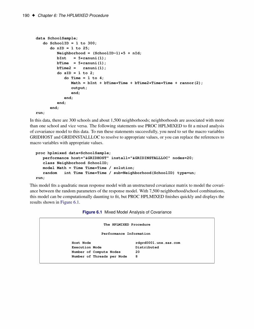
190 F Chapter 6: The HPLMIXED Procedure
data SchoolSample;do SchoolID = 1 to 300;
do nID = 1 to 25;Neighborhood = (SchoolID-1)*5 + nId;bInt = 5*ranuni(1);bTime = 5*ranuni(1);bTime2 = ranuni(1);do sID = 1 to 2;
do Time = 1 to 4;Math = bInt + bTime*Time + bTime2*Time*Time + rannor(2);output;end;
end;end;
end;run;
In this data, there are 300 schools and about 1,500 neighborhoods; neighborhoods are associated with morethan one school and vice versa. The following statements use PROC HPLMIXED to fit a mixed analysisof covariance model to this data. To run these statements successfully, you need to set the macro variablesGRIDHOST and GRIDINSTALLLOC to resolve to appropriate values, or you can replace the references tomacro variables with appropriate values.
proc hplmixed data=SchoolSample;performance host="&GRIDHOST" install="&GRIDINSTALLLOC" nodes=20;class Neighborhood SchoolID;model Math = Time Time*Time / solution;random int Time Time*Time / sub=Neighborhood(SchoolID) type=un;
run;
This model fits a quadratic mean response model with an unstructured covariance matrix to model the covari-ance between the random parameters of the response model. With 7,500 neighborhood/school combinations,this model can be computationally daunting to fit, but PROC HPLMIXED finishes quickly and displays theresults shown in Figure 6.1.
Figure 6.1 Mixed Model Analysis of Covariance
The HPLMIXED Procedure
Performance Information
Host Node rdgrd0001.unx.sas.comExecution Mode DistributedNumber of Compute Nodes 20Number of Threads per Node 8

Mixed Model Analysis of Covariance with Many Groups F 191
Figure 6.1 continued
Model Information
Data Set WORK.SCHOOLSAMPLEDependent Variable MathCovariance Structure UnstructuredSubject Effect Neighborho(SchoolID)Estimation Method Restricted Maximum LikelihoodResidual Variance Method ProfileFixed Effects SE Method Model-BasedDegrees of Freedom Method Residual
Class Level Information
Class Levels Values
Neighborhood 1520 1 2 3 4 5 6 7 8 9 10 11 12 13 14 15 16 17 1819 20 ...
SchoolID 300 1 2 3 4 5 6 7 8 9 10 11 12 13 14 15 16 17 1819 20 ...
Dimensions
Covariance Parameters 7Columns in X 3Columns in Z Per Subject 3Subjects 7500Max Obs Per Subject 8
Number of Observations Read 60000Number of Observations Used 60000Number of Observations Not Used 0Number of Observations Swapped 52500Number of Subjects Needing Swap 7500
Optimization Information
Optimization Technique Newton-Raphson with RidgingParameters in Optimization 6Lower Boundaries 3Upper Boundaries 0Starting Values From Data
Iteration History
Objective MaxIteration Evaluations Function Change Gradient
0 2 225641.67142 . 2.135E-8
Convergence criterion (ABSGCONV=0.00001) satisfied.
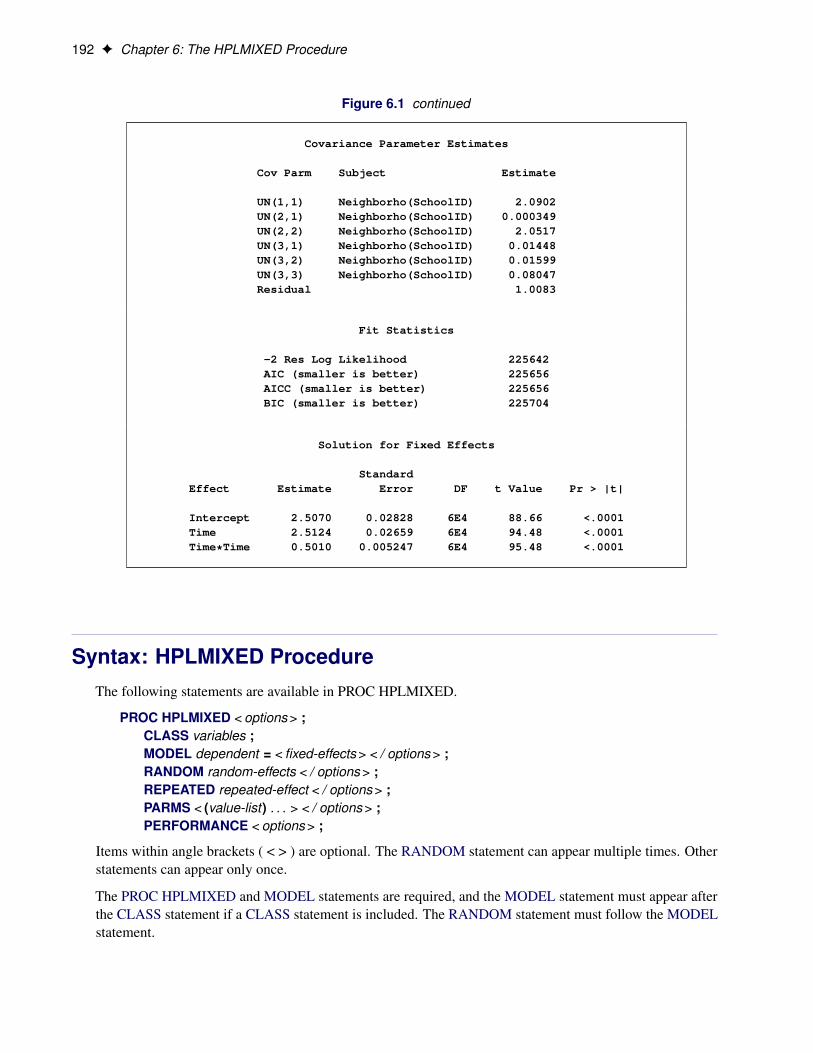
192 F Chapter 6: The HPLMIXED Procedure
Figure 6.1 continued
Covariance Parameter Estimates
Cov Parm Subject Estimate
UN(1,1) Neighborho(SchoolID) 2.0902UN(2,1) Neighborho(SchoolID) 0.000349UN(2,2) Neighborho(SchoolID) 2.0517UN(3,1) Neighborho(SchoolID) 0.01448UN(3,2) Neighborho(SchoolID) 0.01599UN(3,3) Neighborho(SchoolID) 0.08047Residual 1.0083
Fit Statistics
-2 Res Log Likelihood 225642AIC (smaller is better) 225656AICC (smaller is better) 225656BIC (smaller is better) 225704
Solution for Fixed Effects
StandardEffect Estimate Error DF t Value Pr > |t|
Intercept 2.5070 0.02828 6E4 88.66 <.0001Time 2.5124 0.02659 6E4 94.48 <.0001Time*Time 0.5010 0.005247 6E4 95.48 <.0001
Syntax: HPLMIXED ProcedureThe following statements are available in PROC HPLMIXED.
PROC HPLMIXED < options > ;CLASS variables ;MODEL dependent = < fixed-effects > < / options > ;RANDOM random-effects < / options > ;REPEATED repeated-effect < / options > ;PARMS < (value-list) . . . > < / options > ;PERFORMANCE < options > ;
Items within angle brackets ( < > ) are optional. The RANDOM statement can appear multiple times. Otherstatements can appear only once.
The PROC HPLMIXED and MODEL statements are required, and the MODEL statement must appear afterthe CLASS statement if a CLASS statement is included. The RANDOM statement must follow the MODELstatement.
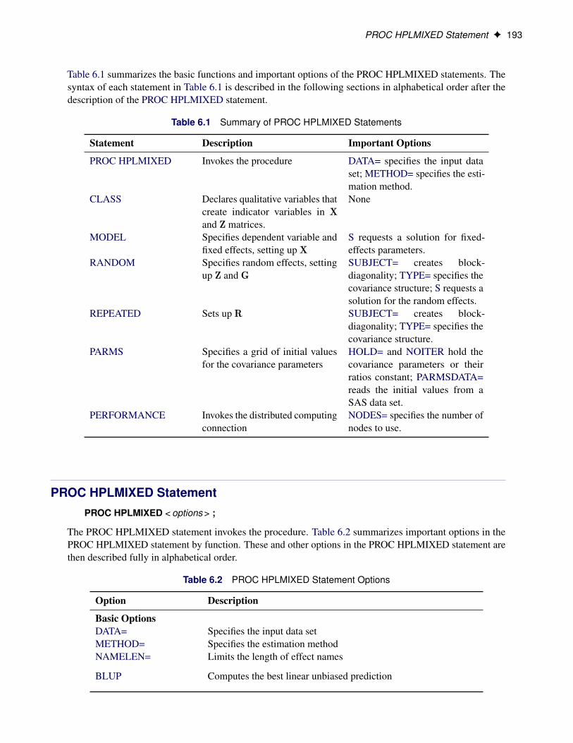
PROC HPLMIXED Statement F 193
Table 6.1 summarizes the basic functions and important options of the PROC HPLMIXED statements. Thesyntax of each statement in Table 6.1 is described in the following sections in alphabetical order after thedescription of the PROC HPLMIXED statement.
Table 6.1 Summary of PROC HPLMIXED Statements
Statement Description Important Options
PROC HPLMIXED Invokes the procedure DATA= specifies the input dataset; METHOD= specifies the esti-mation method.
CLASS Declares qualitative variables thatcreate indicator variables in Xand Z matrices.
None
MODEL Specifies dependent variable andfixed effects, setting up X
S requests a solution for fixed-effects parameters.
RANDOM Specifies random effects, settingup Z and G
SUBJECT= creates block-diagonality; TYPE= specifies thecovariance structure; S requests asolution for the random effects.
REPEATED Sets up R SUBJECT= creates block-diagonality; TYPE= specifies thecovariance structure.
PARMS Specifies a grid of initial valuesfor the covariance parameters
HOLD= and NOITER hold thecovariance parameters or theirratios constant; PARMSDATA=reads the initial values from aSAS data set.
PERFORMANCE Invokes the distributed computingconnection
NODES= specifies the number ofnodes to use.
PROC HPLMIXED StatementPROC HPLMIXED < options > ;
The PROC HPLMIXED statement invokes the procedure. Table 6.2 summarizes important options in thePROC HPLMIXED statement by function. These and other options in the PROC HPLMIXED statement arethen described fully in alphabetical order.
Table 6.2 PROC HPLMIXED Statement Options
Option Description
Basic OptionsDATA= Specifies the input data setMETHOD= Specifies the estimation methodNAMELEN= Limits the length of effect names
BLUP Computes the best linear unbiased prediction

194 F Chapter 6: The HPLMIXED Procedure
Table 6.2 continued
Option Description
Options Related to OutputNOCLPRINT Suppresses the “Class Level Information” table completely or in
partsMAXCLPRINT= Specifies the maximum levels of CLASS variables to print
Optimization OptionsABSCONV= Tunes an absolute function convergence criterionABSFCONV= Tunes an absolute function difference convergence criterionABSGCONV= Tunes the absolute gradient convergence criterionFCONV= Tunes the relative function convergence criterionGCONV= Tunes the relative gradient convergence criterionMAXITER= Chooses the maximum number of iterations in any optimizationMAXFUNC= Specifies the maximum number of function evaluations in any
optimizationMAXTIME= Specifies the upper limit on seconds of CPU time for any optimiza-
tionMINITER= Specifies the minimum number of iterations in any optimizationTECHNIQUE= Selects the optimization techniqueXCONV= Tunes the relative parameter convergence criterion
You can specify the following options in the PROC HPLMIXED statement.
ABSCONV=rspecifies an absolute function convergence criterion. For minimization, termination requires f . .k// �r, where is the vector of parameters in the optimization and f .�/ is the objective function. Thedefault value of r is the negative square root of the largest double-precision value, which serves only asa protection against overflows.
ABSFCONV=rspecifies an absolute function difference convergence criterion. For all techniques except Nelder–Meadsimplex (NMSIMP), termination requires a small change of the function value in successive iterations:
jf . .k�1// � f . .k//j � r
Here, denotes the vector of parameters that participate in the optimization and f .�/ is the objectivefunction. The same formula is used for the NMSIMP technique, but .k/ is defined as the vertex withthe lowest function value and .k�1/ is defined as the vertex with the highest function value in thesimplex. The default value is r D 0.
ABSGCONV=rspecifies an absolute gradient convergence criterion. Termination requires the maximum absolutegradient element to be small:
maxjjgj .
.k//j � r
Here, denotes the vector of parameters that participate in the optimization and gj .�/ is the gradientof the objective function with respect to the j parameter. This criterion is not used by the NMSIMPtechnique. The default value is r=1E–5.

PROC HPLMIXED Statement F 195
BLUP< (suboptions) >requests that best linear unbiased predictions (BLUPs) for the random effects be displayed. To use thisoption, you must also use the PARMS statement to specify fixed values for the covariance parameters.
The BLUP solution might be sensitive to the order of observations, and hence to how the data aredistributed on the grid. If there are multiple measures of a repeated effect, then the BLUP solution isnot unique. If the order of these multiple measures on the grid differs for different runs, then differentBLUP solutions will result.
You can specify the following suboptions:
ITPRINT=number specifies that the iteration history be displayed after every number of iterations.The default value is 10, which means the procedure displays the iteration historyfor every 10 iterations.
MAXITER=number specifies the maximum number of iterations allowed. The default value is thenumber of parameters in the BLUP option plus 2.
TOL=number specifies the tolerance value. The default value is the square root of machineprecision.
DATA=SAS-data-setnames the SAS data set to be used as the input data set. The default is the most recently created dataset.
FCONV=rspecifies a relative function convergence criterion. For all techniques except NMSIMP, terminationrequires a small relative change of the function value in successive iterations,
jf . .k// � f . .k�1//j
jf . .k�1//j� r
Here, denotes the vector of parameters that participate in the optimization and f .�/ is the objectivefunction. The same formula is used for the NMSIMP technique, but .k/ is defined as the vertex withthe lowest function value and .k�1/ is defined as the vertex with the highest function value in thesimplex.
The default is r D 10�FDIGITS, where FDIGITS is � log10.�/ and � is the machine precision.
GCONV=rspecifies a relative gradient convergence criterion. For all techniques except CONGRA and NMSIMP,termination requires that the normalized predicted function reduction be small,
g. .k//0ŒH.k/��1g. .k//jf . .k//j
� r
Here, denotes the vector of parameters that participate in the optimization, f .�/ is the objectivefunction, and g.�/ is the gradient. For the CONGRA technique (where a reliable Hessian estimate H isnot available), the following criterion is used:
k g. .k// k22 k s. .k// k2k g. .k// � g. .k�1// k2 jf . .k//j
� r
This criterion is not used by the NMSIMP technique. The default value is r=1E–8.
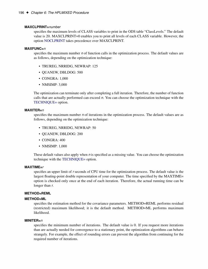
196 F Chapter 6: The HPLMIXED Procedure
MAXCLPRINT=numberspecifies the maximum levels of CLASS variables to print in the ODS table “ClassLevels.” The defaultvalue is 20. MAXCLPRINT=0 enables you to print all levels of each CLASS variable. However, theoption NOCLPRINT takes precedence over MAXCLPRINT.
MAXFUNC=nspecifies the maximum number n of function calls in the optimization process. The default values areas follows, depending on the optimization technique:
• TRUREG, NRRIDG, NEWRAP: 125
• QUANEW, DBLDOG: 500
• CONGRA: 1,000
• NMSIMP: 3,000
The optimization can terminate only after completing a full iteration. Therefore, the number of functioncalls that are actually performed can exceed n. You can choose the optimization technique with theTECHNIQUE= option.
MAXITER=nspecifies the maximum number n of iterations in the optimization process. The default values are asfollows, depending on the optimization technique:
• TRUREG, NRRIDG, NEWRAP: 50
• QUANEW, DBLDOG: 200
• CONGRA: 400
• NMSIMP: 1,000
These default values also apply when n is specified as a missing value. You can choose the optimizationtechnique with the TECHNIQUE= option.
MAXTIME=rspecifies an upper limit of r seconds of CPU time for the optimization process. The default value is thelargest floating-point double representation of your computer. The time specified by the MAXTIME=option is checked only once at the end of each iteration. Therefore, the actual running time can belonger than r.
METHOD=REML
METHOD=MLspecifies the estimation method for the covariance parameters. METHOD=REML performs residual(restricted) maximum likelihood; it is the default method. METHOD=ML performs maximumlikelihood.
MINITER=nspecifies the minimum number of iterations. The default value is 0. If you request more iterationsthan are actually needed for convergence to a stationary point, the optimization algorithms can behavestrangely. For example, the effect of rounding errors can prevent the algorithm from continuing for therequired number of iterations.

PROC HPLMIXED Statement F 197
NAMELEN=numberspecifies the length to which long effect names are shortened. The minimum value is 20, which is alsothe default.
NOCLPRINT< =number >suppresses the display of the “Class Level Information” table if you do not specify number. If youspecify number, the values of the classification variables are displayed for only those variables whosenumber of levels is less than number. Specifying a number helps to reduce the size of the “Class LevelInformation” table if some classification variables have a large number of levels.
NOPRINTsuppresses the generation of ODS output.
SINGCHOL=numbertunes the singularity criterion in Cholesky decompositions. The default is 1E4 times the machineepsilon; this product is approximately 1E–12 on most computers.
SINGSWEEP=numbertunes the singularity criterion for sweep operations. The default is 1E4 times the machine epsilon; thisproduct is approximately 1E–12 on most computers.
SINGULAR=numbertunes the general singularity criterion applied by the HPLMIXED procedure in sweeps and inversions.The default is 1E4 times the machine epsilon; this product is approximately 1E–12 on most computers.
TECHNIQUE=keywordspecifies the optimization technique for obtaining maximum likelihood estimates. You can specify anyof the following keywords:
CONGRA performs a conjugate-gradient optimization.
DBLDOG performs a version of double-dogleg optimization.
NEWRAP performs a Newton-Raphson optimization combining a line-search algorithm withridging.
NMSIMP performs a Nelder-Mead simplex optimization.
NONE performs no optimization.
NRRIDG performs a Newton-Raphson optimization with ridging.
QUANEW performs a dual quasi-Newton optimization.
TRUREG performs a trust-region optimization.
The default value is TECHNIQUE=NRRIDG.
XCONV=rspecifies the relative parameter convergence criterion:
• For all techniques except NMSIMP, termination requires a small relative parameter change insubsequent iterations:
maxj j .k/j �
.k�1/j j
max.j .k/j j; j .k�1/j j/
� r

198 F Chapter 6: The HPLMIXED Procedure
• For the NMSIMP technique, the same formula is used, but .k/j is defined as the vertex with the
lowest function value and .k�1/j is defined as the vertex with the highest function value in thesimplex.
The default value is r = 1E–8 for the NMSIMP technique and r = 0 otherwise.
CLASS StatementCLASS variables ;
The CLASS statement names the classification variables to be used as explanatory variables in the analysis.These variables enter the analysis not through their values, but through levels to which the unique valuesare mapped. See the section “Levelization of Classification Variables” on page 50 of Chapter 3, “SharedStatistical Concepts” for details about these mappings.
If a CLASS statement is specified, it must precede the MODEL statement in high-performance analyticalprocedures that support a MODEL statement.
Levels of classification variables are ordered by their external formatted values, except for numeric variableswith no explicit format, which are ordered by their unformatted (internal) values.
MODEL StatementMODEL dependent = < fixed-effects >< / options > ;
The MODEL statement names a single dependent variable and the fixed effects, which determine the Xmatrix of the mixed model. (For details, see the section “Specification and Parameterization of Model Effects”on page 52 of Chapter 3, “Shared Statistical Concepts”.) The MODEL statement is required.
An intercept is included in the fixed-effects model by default. If no fixed effects are specified, only thisintercept term is fit. The intercept can be removed by using the NOINT option.
Table 6.3 summarizes options in the MODEL statement. These are subsequently discussed in detail inalphabetical order.
Table 6.3 Summary of Important MODEL Statement Options
Option Description
Model BuildingNOINT Excludes the fixed-effect intercept from model
Statistical ComputationsALPHA=˛ Determines the confidence level (1 � ˛) for fixed effectsDDFM= Specifies the method for computing denominator degrees of
freedom
Statistical OutputCL Displays confidence limits for fixed-effects parameter estimatesSOLUTION Displays fixed-effects parameter estimates
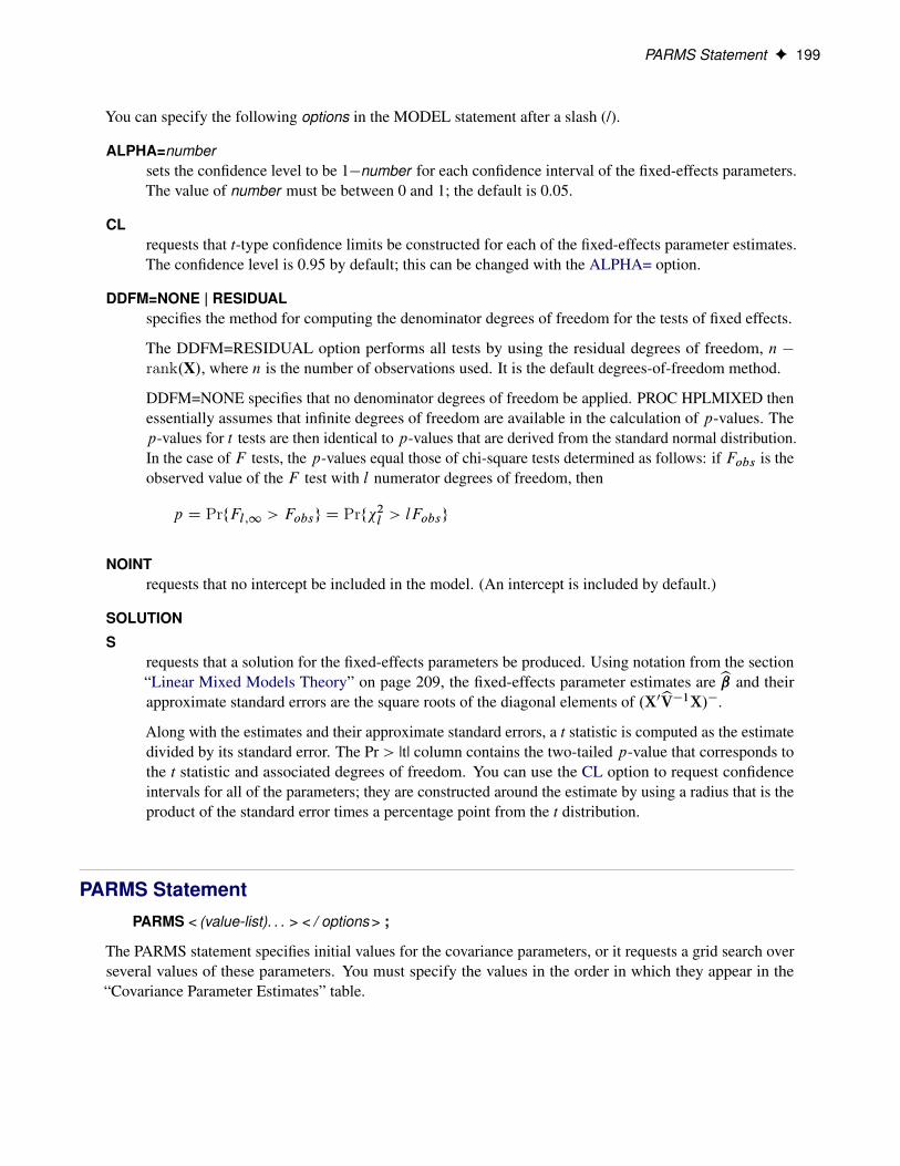
PARMS Statement F 199
You can specify the following options in the MODEL statement after a slash (/).
ALPHA=numbersets the confidence level to be 1�number for each confidence interval of the fixed-effects parameters.The value of number must be between 0 and 1; the default is 0.05.
CLrequests that t-type confidence limits be constructed for each of the fixed-effects parameter estimates.The confidence level is 0.95 by default; this can be changed with the ALPHA= option.
DDFM=NONE | RESIDUALspecifies the method for computing the denominator degrees of freedom for the tests of fixed effects.
The DDFM=RESIDUAL option performs all tests by using the residual degrees of freedom, n �rank.X/, where n is the number of observations used. It is the default degrees-of-freedom method.
DDFM=NONE specifies that no denominator degrees of freedom be applied. PROC HPLMIXED thenessentially assumes that infinite degrees of freedom are available in the calculation of p-values. Thep-values for t tests are then identical to p-values that are derived from the standard normal distribution.In the case of F tests, the p-values equal those of chi-square tests determined as follows: if Fobs is theobserved value of the F test with l numerator degrees of freedom, then
p D PrfFl;1 > Fobsg D Prf�2l > lFobsg
NOINTrequests that no intercept be included in the model. (An intercept is included by default.)
SOLUTION
Srequests that a solution for the fixed-effects parameters be produced. Using notation from the section“Linear Mixed Models Theory” on page 209, the fixed-effects parameter estimates are b and theirapproximate standard errors are the square roots of the diagonal elements of .X0bV�1X/�.
Along with the estimates and their approximate standard errors, a t statistic is computed as the estimatedivided by its standard error. The Pr > |t| column contains the two-tailed p-value that corresponds tothe t statistic and associated degrees of freedom. You can use the CL option to request confidenceintervals for all of the parameters; they are constructed around the estimate by using a radius that is theproduct of the standard error times a percentage point from the t distribution.
PARMS StatementPARMS < (value-list). . . > < / options > ;
The PARMS statement specifies initial values for the covariance parameters, or it requests a grid search overseveral values of these parameters. You must specify the values in the order in which they appear in the“Covariance Parameter Estimates” table.
200 F Chapter 6: The HPLMIXED Procedure
The value-list specification can take any of several forms:
m a single value
m1;m2; : : : ;mn several values
m to n a sequence in which m equals the starting value, n equals the ending value, and theincrement equals 1
m to n by i a sequence in which m equals the starting value, n equals the ending value, and theincrement equals i
m1;m2 to m3 mixed values and sequences
You can use the PARMS statement to input known parameters.
If you specify more than one set of initial values, PROC HPLMIXED performs a grid search of the likelihoodsurface and uses the best point on the grid for subsequent analysis. Specifying a large number of grid pointscan result in long computing times.
The results from the PARMS statement are the values of the parameters on the specified grid (denotedby CovP1 through CovPn), the residual variance (possibly estimated) for models with a residual varianceparameter, and various functions of the likelihood.
You can specify the following options in the PARMS statement after a slash (/).
HOLD=all
EQCONS=allspecifies that all parameter values be held to equal the specified values.
For example, the following statement constrains all covariance parameters to equal 5, 3, 2, and 3:
parms (5) (3) (2) (3) / hold=all;
LOWERB=value-listenables you to specify lower boundary constraints on the covariance parameters. The value-listspecification is a list of numbers or missing values (.) separated by commas. You must list the numbersin the order that PROC HPLMIXED uses for the covariance parameters, and each number correspondsto the lower boundary constraint. A missing value instructs PROC HPLMIXED to use its defaultconstraint. If you do not specify numbers for all of the covariance parameters, PROC HPLMIXEDassumes the remaining ones are missing.
This option is useful when you want to constrain the G matrix to be positive definite in order to avoidthe more computationally intensive algorithms that would be required when G becomes singular. Thecorresponding statements for a random coefficients model are as follows:
proc hplmixed;class person;model y = time;random int time / type=fa0(2) sub=person;parms / lowerb=1e-4,.,1e-4;
run;

PERFORMANCE Statement F 201
The TYPE=FA0(2) structure specifies a Cholesky root parameterization for the 2 � 2 unstructuredblocks in G. This parameterization ensures that the G matrix is nonnegative definite, and the PARMSstatement then ensures that it is positive definite by constraining the two diagonal terms to be greaterthan or equal to 1E–4.
NOITERrequests that no optimization iterations be performed and that PROC HPLMIXED use the best valuefrom the grid search to perform inferences. By default, iterations begin at the best value from thePARMS grid search.
PARMSDATA=SAS-data-set
PDATA=SAS-data-setreads in covariance parameter values from a SAS data set. The data set should contain the Est or Covp1through Covpn variables.
UPPERB=value-listenables you to specify upper boundary constraints on the covariance parameters. The value-listspecification is a list of numbers or missing values (.) separated by commas. You must list the numbersin the order that PROC HPLMIXED uses for the covariance parameters, and each number correspondsto the upper boundary constraint. A missing value instructs PROC HPLMIXED to use its defaultconstraint. If you do not specify numbers for all of the covariance parameters, PROC HPLMIXEDassumes that the remaining ones are missing.
PERFORMANCE StatementPERFORMANCE < performance-options > ;
The PERFORMANCE statement defines performance parameters for multithreaded and distributed comput-ing, passes variables about the distributed computing environment, and requests detailed results about theperformance characteristics of a SAS high-performance analytical procedure.
You can also use the PERFORMANCE statement to control whether a SAS high-performance analyticalprocedure executes in single-machine mode or distributed mode.
The PERFORMANCE statement for SAS high-performance analytical procedures is documented in thesection “PERFORMANCE Statement” on page 34 of Chapter 2, “Shared Concepts and Topics.”
RANDOM StatementRANDOM random-effects < / options > ;
The RANDOM statement defines the random effects that constitute the vector in the mixed model. Youcan use this statement to specify traditional variance component models and to specify random coefficients.The random effects can be classification or continuous, and multiple RANDOM statements are possible.
Using notation from the section “Linear Mixed Models Theory” on page 209, the purpose of the RANDOMstatement is to define the Z matrix of the mixed model, the random effects in the vector, and the structureof G. The Z matrix is constructed exactly as the X matrix for the fixed effects is constructed, and the G
202 F Chapter 6: The HPLMIXED Procedure
matrix is constructed to correspond with the effects that constitute Z. The structure of G is defined by usingthe TYPE= option.
You can specify INTERCEPT (or INT) as a random effect to indicate the intercept. PROC HPLMIXED doesnot include the intercept in the RANDOM statement by default as it does in the MODEL statement.
Table 6.4 summarizes important options in the RANDOM statement. All options are subsequently discussedin alphabetical order.
Table 6.4 Summary of Important RANDOM Statement Options
Option Description
Construction of Covariance StructureSUBJECT= Identifies the subjects in the modelTYPE= Specifies the covariance structure
Statistical OutputALPHA=˛ Determines the confidence level (1 � ˛)CL Requests confidence limits for predictors of random effectsSOLUTION Displays solutionsb of the random effects
You can specify the following options in the RANDOM statement after a slash (/).
ALPHA=numbersets the confidence level to be 1�number for each confidence interval of the random-effects estimates.The value of number must be between 0 and 1; the default is 0.05.
CLrequests that t-type confidence limits be constructed for each of the random-effect estimates. Theconfidence level is 0.95 by default; this can be changed with the ALPHA= option.
SOLUTION
Srequests that the solution for the random-effects parameters be produced. Using notation from thesection “Linear Mixed Models Theory” on page 209, these estimates are the empirical best linearunbiased predictors (EBLUPs),b D bGZ0bV�1.y�Xb/. They can be useful for comparing the randomeffects from different experimental units and can also be treated as residuals in performing diagnosticsfor your mixed model.
The numbers displayed in the SE Pred column of the “Solution for Random Effects” table are notthe standard errors of theb displayed in the Estimate column; rather, they are the standard errors ofpredictionsb i � i , whereb i is the ith EBLUP and i is the ith random-effect parameter.
SUBJECT=effect
SUB=effectidentifies the subjects in your mixed model. Complete independence is assumed across subjects; thus,for the RANDOM statement, the SUBJECT= option produces a block-diagonal structure in G withidentical blocks. In fact, specifying a subject effect is equivalent to nesting all other effects in theRANDOM statement within the subject effect.
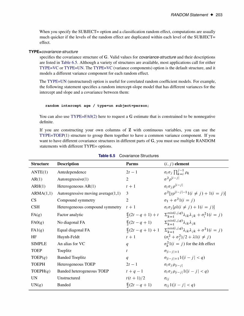
RANDOM Statement F 203
When you specify the SUBJECT= option and a classification random effect, computations are usuallymuch quicker if the levels of the random effect are duplicated within each level of the SUBJECT=effect.
TYPE=covariance-structurespecifies the covariance structure of G. Valid values for covariance-structure and their descriptionsare listed in Table 6.5. Although a variety of structures are available, most applications call for eitherTYPE=VC or TYPE=UN. The TYPE=VC (variance components) option is the default structure, and itmodels a different variance component for each random effect.
The TYPE=UN (unstructured) option is useful for correlated random coefficient models. For example,the following statement specifies a random intercept-slope model that has different variances for theintercept and slope and a covariance between them:
random intercept age / type=un subject=person;
You can also use TYPE=FA0(2) here to request a G estimate that is constrained to be nonnegativedefinite.
If you are constructing your own columns of Z with continuous variables, you can use theTYPE=TOEP(1) structure to group them together to have a common variance component. If youwant to have different covariance structures in different parts of G, you must use multiple RANDOMstatements with different TYPE= options.
Table 6.5 Covariance Structures
Structure Description Parms .i; j / element
ANTE(1) Antedependence 2t � 1 �i�jQj�1
kDi�k
AR(1) Autoregressive(1) 2 �2�ji�j j
ARH(1) Heterogeneous AR(1) t C 1 �i�j�ji�j j
ARMA(1,1) Autoregressive moving average(1,1) 3 �2Œ �ji�j j�11.i ¤ j /C 1.i D j /�
CS Compound symmetry 2 �1 C �21.i D j /
CSH Heterogeneous compound symmetry t C 1 �i�j Œ�1.i ¤ j /C 1.i D j /�
FA(q) Factor analytic q2.2t � q C 1/C t †
min.i;j;q/kD1
�ik�jk C �2i 1.i D j /
FA0(q) No diagonal FA q2.2t � q C 1/ †
min.i;j;q/kD1
�ik�jk
FA1(q) Equal diagonal FA q2.2t � q C 1/C 1 †
min.i;j;q/kD1
�ik�jk C �21.i D j /
HF Huynh-Feldt t C 1 .�2i C �2j /=2C �1.i ¤ j /
SIMPLE An alias for VC q �2k1.i D j / for the kth effect
TOEP Toeplitz t �ji�j jC1
TOEP(q) Banded Toeplitz q �ji�j jC11.ji � j j < q/
TOEPH Heterogeneous TOEP 2t � 1 �i�j�ji�j j
TOEPH(q) Banded heterogeneous TOEP t C q � 1 �i�j�ji�j j1.ji � j j < q/
UN Unstructured t .t C 1/=2 �ij
UN(q) Banded q2.2t � q C 1/ �ij 1.ji � j j < q/
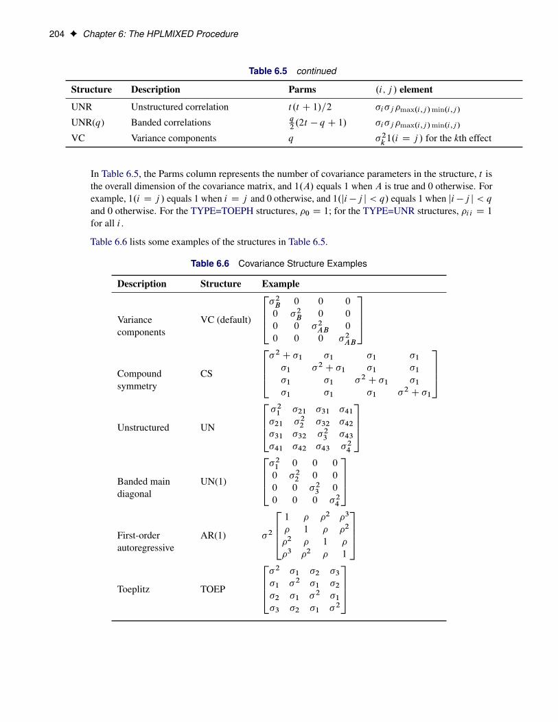
204 F Chapter 6: The HPLMIXED Procedure
Table 6.5 continued
Structure Description Parms .i; j / element
UNR Unstructured correlation t .t C 1/=2 �i�j�max.i;j /min.i;j /
UNR(q) Banded correlations q2.2t � q C 1/ �i�j�max.i;j /min.i;j /
VC Variance components q �2k1.i D j / for the kth effect
In Table 6.5, the Parms column represents the number of covariance parameters in the structure, t isthe overall dimension of the covariance matrix, and 1.A/ equals 1 when A is true and 0 otherwise. Forexample, 1.i D j / equals 1 when i D j and 0 otherwise, and 1.ji�j j < q/ equals 1 when ji�j j < qand 0 otherwise. For the TYPE=TOEPH structures, �0 D 1; for the TYPE=UNR structures, �i i D 1for all i .
Table 6.6 lists some examples of the structures in Table 6.5.
Table 6.6 Covariance Structure Examples
Description Structure Example
Variancecomponents
VC (default)
2664�2B 0 0 0
0 �2B 0 0
0 0 �2AB 0
0 0 0 �2AB
3775
Compoundsymmetry
CS
2664�2 C �1 �1 �1 �1�1 �2 C �1 �1 �1�1 �1 �2 C �1 �1�1 �1 �1 �2 C �1
3775
Unstructured UN
2664�21 �21 �31 �41�21 �22 �32 �42�31 �32 �23 �43�41 �42 �43 �24
3775
Banded maindiagonal
UN(1)
2664�21 0 0 0
0 �22 0 0
0 0 �23 0
0 0 0 �24
3775
First-orderautoregressive
AR(1) �2
26641 � �2 �3
� 1 � �2
�2 � 1 �
�3 �2 � 1
3775
Toeplitz TOEP
2664�2 �1 �2 �3�1 �2 �1 �2�2 �1 �2 �1�3 �2 �1 �2
3775
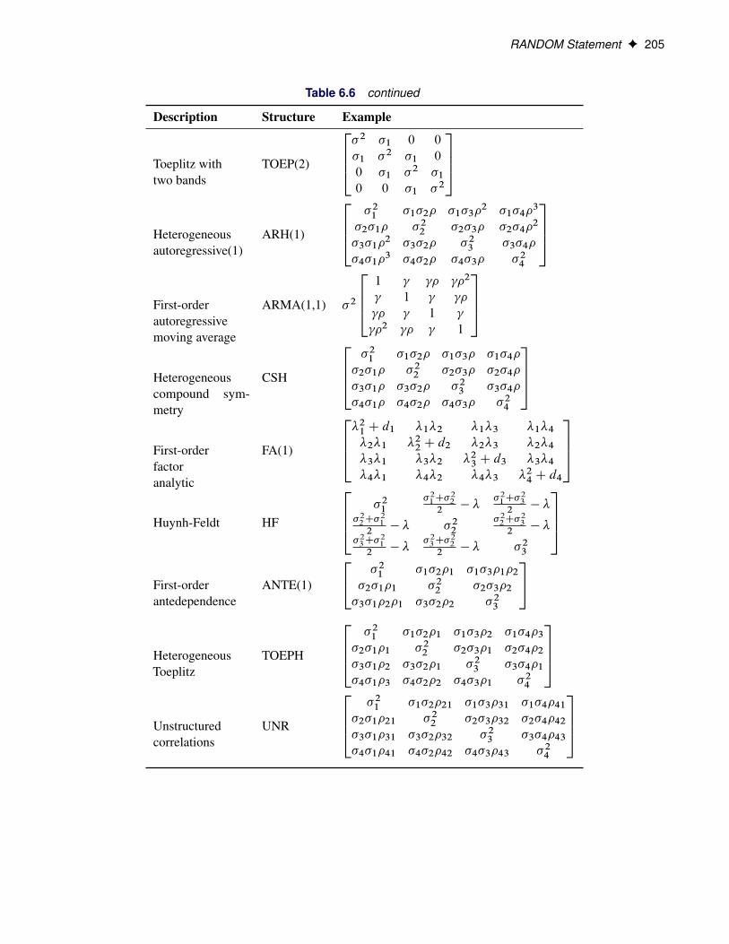
RANDOM Statement F 205
Table 6.6 continued
Description Structure Example
Toeplitz withtwo bands
TOEP(2)
2664�2 �1 0 0
�1 �2 �1 0
0 �1 �2 �10 0 �1 �2
3775
Heterogeneousautoregressive(1)
ARH(1)
2664�21 �1�2� �1�3�
2 �1�4�3
�2�1� �22 �2�3� �2�4�2
�3�1�2 �3�2� �23 �3�4�
�4�1�3 �4�2� �4�3� �24
3775
First-orderautoregressivemoving average
ARMA(1,1) �2
26641 � �2
1 �
� 1
�2 � 1
3775
Heterogeneouscompound sym-metry
CSH
2664�21 �1�2� �1�3� �1�4�
�2�1� �22 �2�3� �2�4�
�3�1� �3�2� �23 �3�4�
�4�1� �4�2� �4�3� �24
3775
First-orderfactoranalytic
FA(1)
2664�21 C d1 �1�2 �1�3 �1�4�2�1 �22 C d2 �2�3 �2�4�3�1 �3�2 �23 C d3 �3�4�4�1 �4�2 �4�3 �24 C d4
3775
Huynh-Feldt HF
2664 �21�21C�
22
2� �
�21C�23
2� �
�22C�21
2� � �22
�22C�23
2� �
�23C�21
2� �
�23C�22
2� � �23
3775First-orderantedependence
ANTE(1)
24 �21 �1�2�1 �1�3�1�2�2�1�1 �22 �2�3�2�3�1�2�1 �3�2�2 �23
35
HeterogeneousToeplitz
TOEPH
2664�21 �1�2�1 �1�3�2 �1�4�3
�2�1�1 �22 �2�3�1 �2�4�2�3�1�2 �3�2�1 �23 �3�4�1�4�1�3 �4�2�2 �4�3�1 �24
3775
Unstructuredcorrelations
UNR
2664�21 �1�2�21 �1�3�31 �1�4�41
�2�1�21 �22 �2�3�32 �2�4�42�3�1�31 �3�2�32 �23 �3�4�43�4�1�41 �4�2�42 �4�3�43 �24
3775

206 F Chapter 6: The HPLMIXED Procedure
The following list provides some further information about these covariance structures:
TYPE=ANTE(1) specifies the first-order antedependence structure (Kenward 1987; Patel 1991;Macchiavelli and Arnold 1994). In Table 6.5, �2i is the i variance parameter, and�k is the k autocorrelation parameter that satisfies j�kj < 1.
TYPE=AR(1) specifies a first-order autoregressive structure. PROC HPLMIXED imposes theconstraint j�j < 1 for stationarity.
TYPE=ARH(1) specifies a heterogeneous first-order autoregressive structure. As withTYPE=AR(1), PROC HPLMIXED imposes the constraint j�j < 1 for stationarity.
TYPE=ARMA(1,1) specifies the first-order autoregressive moving average structure. In Table 6.5, �is the autoregressive parameter, models a moving average component, and �2 isthe residual variance. In the notation of Fuller (1976, p. 68), � D �1 and
D.1C b1�1/.�1 C b1/
1C b21 C 2b1�1
The example in Table 6.6 and jb1j < 1 imply that
b1 Dˇ �
pˇ2 � 4˛2
2˛
where ˛ D � � and ˇ D 1 C �2 � 2 �. PROC HPLMIXED imposes theconstraints j�j < 1 and j j < 1 for stationarity, although the resulting covariancematrix is not positive definite for some values of � and in this region. When theestimated value of � becomes negative, the computed covariance is multiplied bycos.�dij / to account for the negativity.
TYPE=CS specifies the compound-symmetry structure, which has constant variance and con-stant covariance.
TYPE=CSH specifies the heterogeneous compound-symmetry structure. This structure has adifferent variance parameter for each diagonal element, and it uses the square rootsof these parameters in the off-diagonal entries. In Table 6.5, �2i is the i varianceparameter, and � is the correlation parameter that satisfies j�j < 1.
TYPE=FA(q) specifies the factor-analytic structure with q factors (Jennrich and Schluchter 1986).This structure is of the form ƒƒ0 C D, where ƒ is a t � q rectangular matrix andD is a t � t diagonal matrix with t different parameters. When q > 1, the elementsof ƒ in its upper right corner (that is, the elements in the i row and j column forj > i) are set to zero to fix the rotation of the structure.
TYPE=FA0(q) is similar to the FA(q) structure except that no diagonal matrix D is included. Whenq < t (that is, when the number of factors is less than the dimension of the matrix),this structure is nonnegative definite but not of full rank. In this situation, you canuse this structure for approximating an unstructured G matrix in the RANDOMstatement. When q D t , you can use this structure to constrain G to be nonnegativedefinite in the RANDOM statement.
TYPE=FA1(q) is similar to the TYPE=FA(q) structure except that all of the elements in D areconstrained to be equal. This offers a useful and more parsimonious alternative tothe full factor-analytic structure.
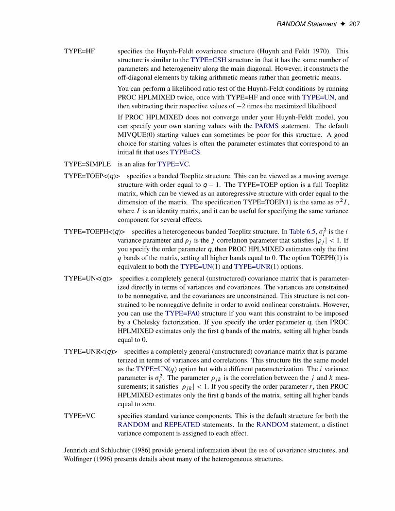
RANDOM Statement F 207
TYPE=HF specifies the Huynh-Feldt covariance structure (Huynh and Feldt 1970). Thisstructure is similar to the TYPE=CSH structure in that it has the same number ofparameters and heterogeneity along the main diagonal. However, it constructs theoff-diagonal elements by taking arithmetic means rather than geometric means.
You can perform a likelihood ratio test of the Huynh-Feldt conditions by runningPROC HPLMIXED twice, once with TYPE=HF and once with TYPE=UN, andthen subtracting their respective values of �2 times the maximized likelihood.
If PROC HPLMIXED does not converge under your Huynh-Feldt model, youcan specify your own starting values with the PARMS statement. The defaultMIVQUE(0) starting values can sometimes be poor for this structure. A goodchoice for starting values is often the parameter estimates that correspond to aninitial fit that uses TYPE=CS.
TYPE=SIMPLE is an alias for TYPE=VC.
TYPE=TOEP<(q)> specifies a banded Toeplitz structure. This can be viewed as a moving averagestructure with order equal to q � 1. The TYPE=TOEP option is a full Toeplitzmatrix, which can be viewed as an autoregressive structure with order equal to thedimension of the matrix. The specification TYPE=TOEP(1) is the same as �2I ,where I is an identity matrix, and it can be useful for specifying the same variancecomponent for several effects.
TYPE=TOEPH<(q)> specifies a heterogeneous banded Toeplitz structure. In Table 6.5, �2i is the ivariance parameter and �j is the j correlation parameter that satisfies j�j j < 1. Ifyou specify the order parameter q, then PROC HPLMIXED estimates only the firstq bands of the matrix, setting all higher bands equal to 0. The option TOEPH(1) isequivalent to both the TYPE=UN(1) and TYPE=UNR(1) options.
TYPE=UN<(q)> specifies a completely general (unstructured) covariance matrix that is parameter-ized directly in terms of variances and covariances. The variances are constrainedto be nonnegative, and the covariances are unconstrained. This structure is not con-strained to be nonnegative definite in order to avoid nonlinear constraints. However,you can use the TYPE=FA0 structure if you want this constraint to be imposedby a Cholesky factorization. If you specify the order parameter q, then PROCHPLMIXED estimates only the first q bands of the matrix, setting all higher bandsequal to 0.
TYPE=UNR<(q)> specifies a completely general (unstructured) covariance matrix that is parame-terized in terms of variances and correlations. This structure fits the same modelas the TYPE=UN(q) option but with a different parameterization. The i varianceparameter is �2i . The parameter �jk is the correlation between the j and k mea-surements; it satisfies j�jkj < 1. If you specify the order parameter r , then PROCHPLMIXED estimates only the first q bands of the matrix, setting all higher bandsequal to zero.
TYPE=VC specifies standard variance components. This is the default structure for both theRANDOM and REPEATED statements. In the RANDOM statement, a distinctvariance component is assigned to each effect.
Jennrich and Schluchter (1986) provide general information about the use of covariance structures, andWolfinger (1996) presents details about many of the heterogeneous structures.
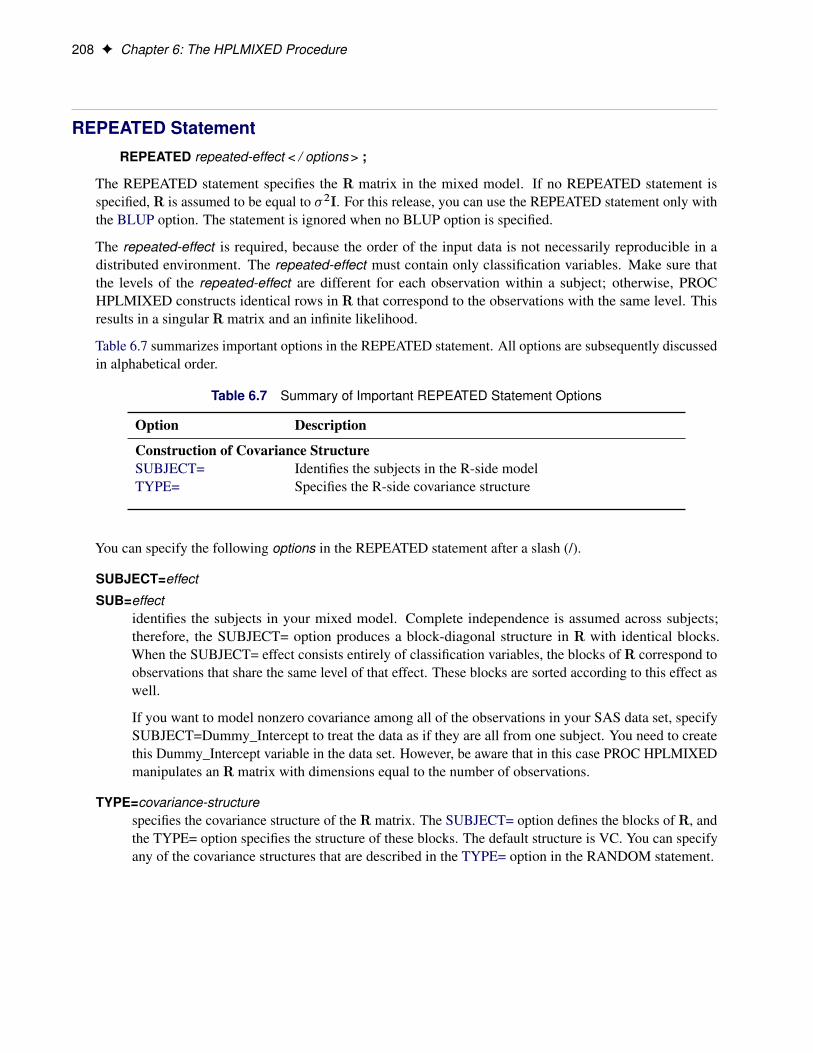
208 F Chapter 6: The HPLMIXED Procedure
REPEATED StatementREPEATED repeated-effect < / options > ;
The REPEATED statement specifies the R matrix in the mixed model. If no REPEATED statement isspecified, R is assumed to be equal to �2I. For this release, you can use the REPEATED statement only withthe BLUP option. The statement is ignored when no BLUP option is specified.
The repeated-effect is required, because the order of the input data is not necessarily reproducible in adistributed environment. The repeated-effect must contain only classification variables. Make sure thatthe levels of the repeated-effect are different for each observation within a subject; otherwise, PROCHPLMIXED constructs identical rows in R that correspond to the observations with the same level. Thisresults in a singular R matrix and an infinite likelihood.
Table 6.7 summarizes important options in the REPEATED statement. All options are subsequently discussedin alphabetical order.
Table 6.7 Summary of Important REPEATED Statement Options
Option Description
Construction of Covariance StructureSUBJECT= Identifies the subjects in the R-side modelTYPE= Specifies the R-side covariance structure
You can specify the following options in the REPEATED statement after a slash (/).
SUBJECT=effect
SUB=effectidentifies the subjects in your mixed model. Complete independence is assumed across subjects;therefore, the SUBJECT= option produces a block-diagonal structure in R with identical blocks.When the SUBJECT= effect consists entirely of classification variables, the blocks of R correspond toobservations that share the same level of that effect. These blocks are sorted according to this effect aswell.
If you want to model nonzero covariance among all of the observations in your SAS data set, specifySUBJECT=Dummy_Intercept to treat the data as if they are all from one subject. You need to createthis Dummy_Intercept variable in the data set. However, be aware that in this case PROC HPLMIXEDmanipulates an R matrix with dimensions equal to the number of observations.
TYPE=covariance-structurespecifies the covariance structure of the R matrix. The SUBJECT= option defines the blocks of R, andthe TYPE= option specifies the structure of these blocks. The default structure is VC. You can specifyany of the covariance structures that are described in the TYPE= option in the RANDOM statement.
Details: HPLMIXED Procedure F 209
Details: HPLMIXED Procedure
Linear Mixed Models TheoryThis section provides an overview of a likelihood-based approach to linear mixed models. This approachsimplifies and unifies many common statistical analyses, including those that involve repeated measures,random effects, and random coefficients. The basic assumption is that the data are linearly related tounobserved multivariate normal random variables. For extensions to nonlinear and nonnormal situations, seethe documentation of the GLIMMIX and NLMIXED procedures in the SAS/STAT User’s Guide. Additionaltheory and examples are provided in Littell et al. (2006), Verbeke and Molenberghs (1997, 2000), and Brownand Prescott (1999).
Matrix Notation
Suppose that you observe n data points y1; : : : ; yn and that you want to explain them by using n values foreach of p explanatory variables x11; : : : ; x1p , x21; : : : ; x2p , : : : ; xn1; : : : ; xnp . The xij values can be eitherregression-type continuous variables or dummy variables that indicate class membership. The standard linearmodel for this setup is
yi D
pXjD1
xijˇj C �i i D 1; : : : ; n
where ˇ1; : : : ; ˇp are unknown fixed-effects parameters to be estimated and �1; : : : ; �n are unknown inde-pendent and identically distributed normal (Gaussian) random variables with mean 0 and variance �2.
The preceding equations can be written simultaneously by using vectors and a matrix, as follows:26664y1y2:::
yn
37775 D26664x11 x12 : : : x1px21 x22 : : : x2p:::
::::::
xn1 xn2 : : : xnp
3777526664ˇ1ˇ2:::
ˇp
37775C26664�1�2:::
�n
37775For convenience, simplicity, and extendability, this entire system is written as
y D Xˇ C �
where y denotes the vector of observed yi ’s, X is the known matrix of xij ’s, ˇ is the unknown fixed-effectsparameter vector, and � is the unobserved vector of independent and identically distributed Gaussian randomerrors.
In addition to denoting data, random variables, and explanatory variables in the preceding fashion, thesubsequent development makes use of basic matrix operators such as transpose (0), inverse (�1), generalizedinverse (�), determinant (j � j), and matrix multiplication. See Searle (1982) for details about these and othermatrix techniques.
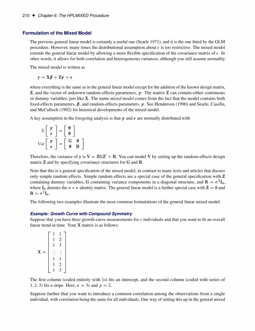
210 F Chapter 6: The HPLMIXED Procedure
Formulation of the Mixed Model
The previous general linear model is certainly a useful one (Searle 1971), and it is the one fitted by the GLMprocedure. However, many times the distributional assumption about � is too restrictive. The mixed modelextends the general linear model by allowing a more flexible specification of the covariance matrix of �. Inother words, it allows for both correlation and heterogeneous variances, although you still assume normality.
The mixed model is written as
y D Xˇ C Z C �
where everything is the same as in the general linear model except for the addition of the known design matrix,Z, and the vector of unknown random-effects parameters, . The matrix Z can contain either continuousor dummy variables, just like X. The name mixed model comes from the fact that the model contains bothfixed-effects parameters, ˇ, and random-effects parameters, . See Henderson (1990) and Searle, Casella,and McCulloch (1992) for historical developments of the mixed model.
A key assumption in the foregoing analysis is that and � are normally distributed with
E�
�
�D
�00
�Var
�
�
�D
�G 00 R
�Therefore, the variance of y is V D ZGZ0 CR. You can model V by setting up the random-effects designmatrix Z and by specifying covariance structures for G and R.
Note that this is a general specification of the mixed model, in contrast to many texts and articles that discussonly simple random effects. Simple random effects are a special case of the general specification with Zcontaining dummy variables, G containing variance components in a diagonal structure, and R D �2In,where In denotes the n� n identity matrix. The general linear model is a further special case with Z D 0 andR D �2In.
The following two examples illustrate the most common formulations of the general linear mixed model.
Example: Growth Curve with Compound SymmetrySuppose that you have three growth curve measurements for s individuals and that you want to fit an overalllinear trend in time. Your X matrix is as follows:
X D
26666666664
1 1
1 2
1 3:::
:::
1 1
1 2
1 3
37777777775The first column (coded entirely with 1s) fits an intercept, and the second column (coded with series of1; 2; 3) fits a slope. Here, n D 3s and p D 2.
Suppose further that you want to introduce a common correlation among the observations from a singleindividual, with correlation being the same for all individuals. One way of setting this up in the general mixed
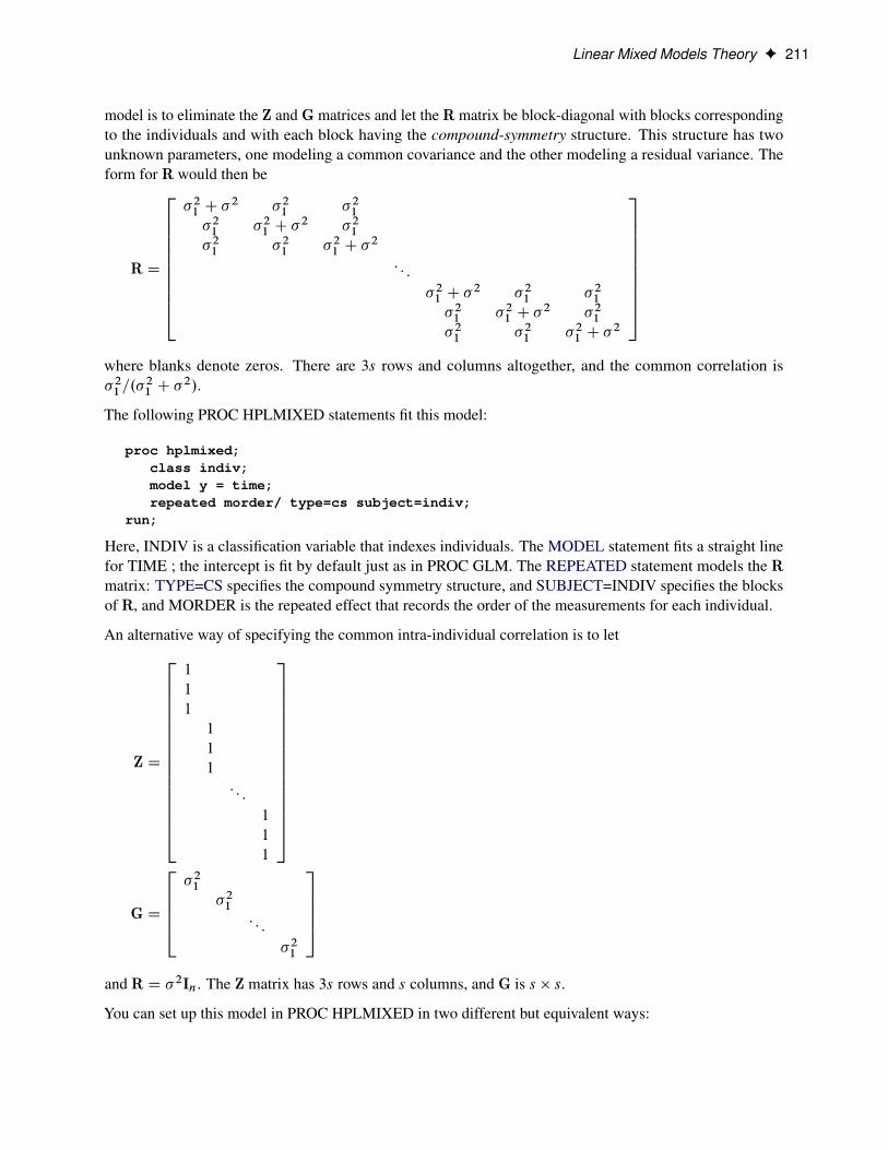
Linear Mixed Models Theory F 211
model is to eliminate the Z and G matrices and let the R matrix be block-diagonal with blocks correspondingto the individuals and with each block having the compound-symmetry structure. This structure has twounknown parameters, one modeling a common covariance and the other modeling a residual variance. Theform for R would then be
R D
26666666664
�21 C �2 �21 �21
�21 �21 C �2 �21
�21 �21 �21 C �2
: : :
�21 C �2 �21 �21
�21 �21 C �2 �21
�21 �21 �21 C �2
37777777775where blanks denote zeros. There are 3s rows and columns altogether, and the common correlation is�21=.�
21 C �
2/.
The following PROC HPLMIXED statements fit this model:
proc hplmixed;class indiv;model y = time;repeated morder/ type=cs subject=indiv;
run;
Here, INDIV is a classification variable that indexes individuals. The MODEL statement fits a straight linefor TIME ; the intercept is fit by default just as in PROC GLM. The REPEATED statement models the Rmatrix: TYPE=CS specifies the compound symmetry structure, and SUBJECT=INDIV specifies the blocksof R, and MORDER is the repeated effect that records the order of the measurements for each individual.
An alternative way of specifying the common intra-individual correlation is to let
Z D
26666666666666664
1
1
1
1
1
1: : :
1
1
1
37777777777777775
G D
26664�21
�21: : :
�21
37775and R D �2In. The Z matrix has 3s rows and s columns, and G is s � s.
You can set up this model in PROC HPLMIXED in two different but equivalent ways:
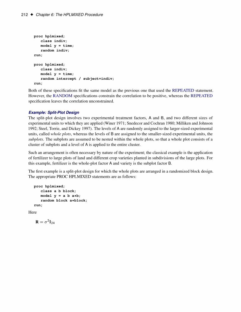
212 F Chapter 6: The HPLMIXED Procedure
proc hplmixed;class indiv;model y = time;random indiv;
run;
proc hplmixed;class indiv;model y = time;random intercept / subject=indiv;
run;
Both of these specifications fit the same model as the previous one that used the REPEATED statement.However, the RANDOM specifications constrain the correlation to be positive, whereas the REPEATEDspecification leaves the correlation unconstrained.
Example: Split-Plot DesignThe split-plot design involves two experimental treatment factors, A and B, and two different sizes ofexperimental units to which they are applied (Winer 1971; Snedecor and Cochran 1980; Milliken and Johnson1992; Steel, Torrie, and Dickey 1997). The levels of A are randomly assigned to the larger-sized experimentalunits, called whole plots, whereas the levels of B are assigned to the smaller-sized experimental units, thesubplots. The subplots are assumed to be nested within the whole plots, so that a whole plot consists of acluster of subplots and a level of A is applied to the entire cluster.
Such an arrangement is often necessary by nature of the experiment; the classical example is the applicationof fertilizer to large plots of land and different crop varieties planted in subdivisions of the large plots. Forthis example, fertilizer is the whole-plot factor A and variety is the subplot factor B.
The first example is a split-plot design for which the whole plots are arranged in a randomized block design.The appropriate PROC HPLMIXED statements are as follows:
proc hplmixed;class a b block;model y = a b a*b;random block a*block;
run;
Here
R D �2I24
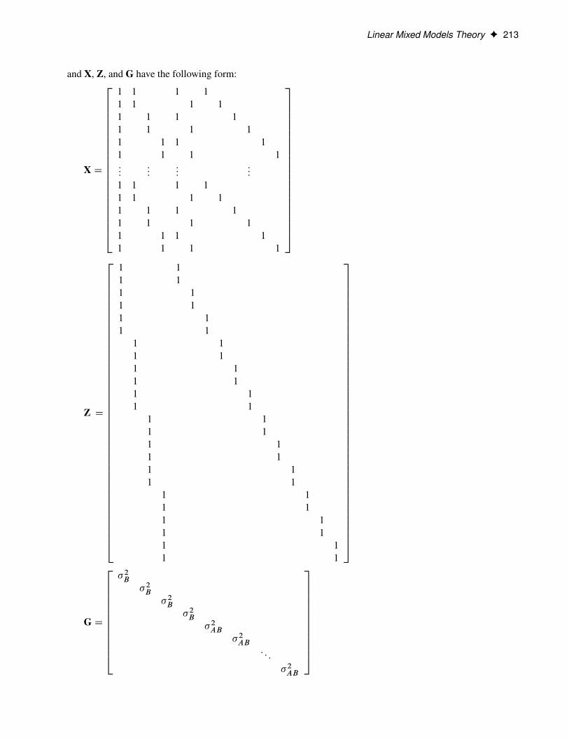
Linear Mixed Models Theory F 213
and X, Z, and G have the following form:
X D
26666666666666666666664
1 1 1 1
1 1 1 1
1 1 1 1
1 1 1 1
1 1 1 1
1 1 1 1:::
::::::
:::
1 1 1 1
1 1 1 1
1 1 1 1
1 1 1 1
1 1 1 1
1 1 1 1
37777777777777777777775
Z D
266666666666666666666666666666666666666666664
1 1
1 1
1 1
1 1
1 1
1 1
1 1
1 1
1 1
1 1
1 1
1 1
1 1
1 1
1 1
1 1
1 1
1 1
1 1
1 1
1 1
1 1
1 1
1 1
377777777777777777777777777777777777777777775
G D
2666666666664
�2B�2B
�2B�2B
�2AB�2AB
: : :
�2AB
3777777777775
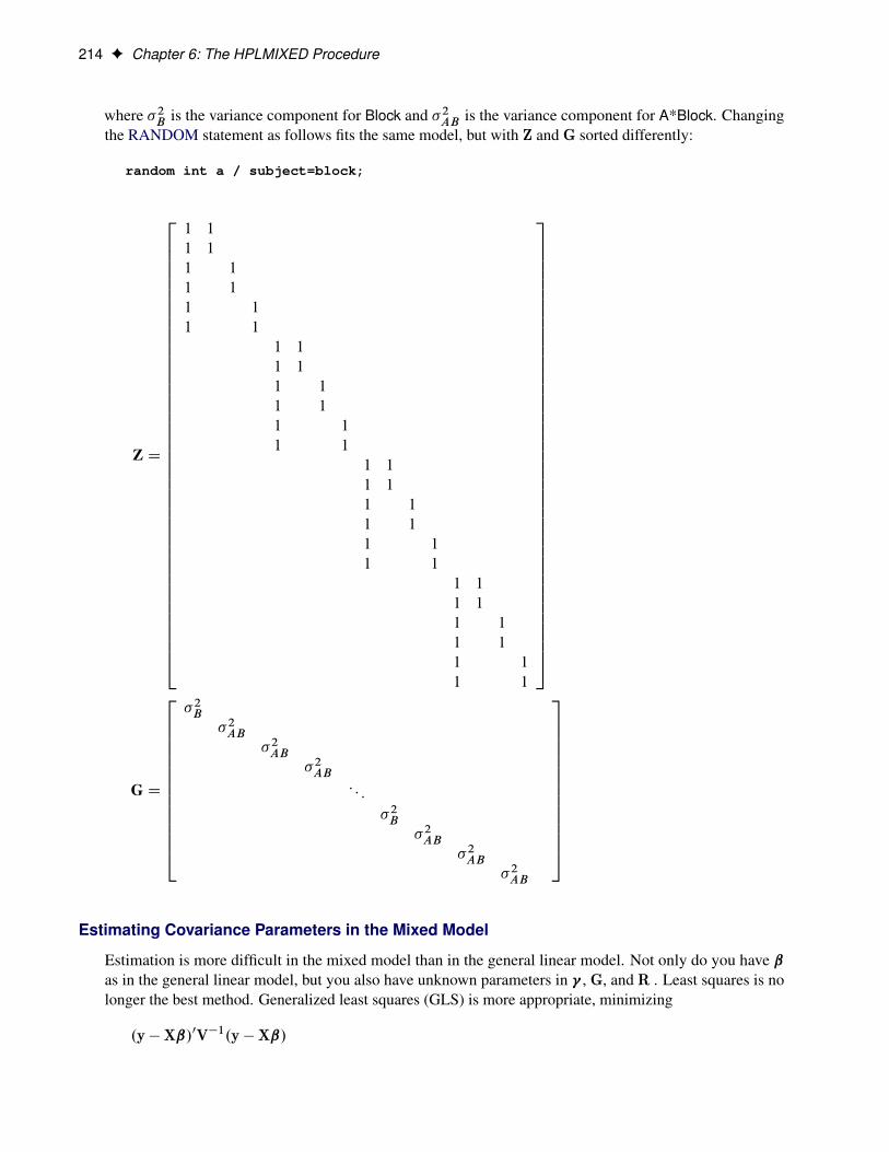
214 F Chapter 6: The HPLMIXED Procedure
where �2B is the variance component for Block and �2AB is the variance component for A*Block. Changingthe RANDOM statement as follows fits the same model, but with Z and G sorted differently:
random int a / subject=block;
Z D
266666666666666666666666666666666666666666664
1 1
1 1
1 1
1 1
1 1
1 1
1 1
1 1
1 1
1 1
1 1
1 1
1 1
1 1
1 1
1 1
1 1
1 1
1 1
1 1
1 1
1 1
1 1
1 1
377777777777777777777777777777777777777777775
G D
266666666666664
�2B�2AB
�2AB�2AB
: : :
�2B�2AB
�2AB�2AB
377777777777775
Estimating Covariance Parameters in the Mixed Model
Estimation is more difficult in the mixed model than in the general linear model. Not only do you have ˇas in the general linear model, but you also have unknown parameters in , G, and R . Least squares is nolonger the best method. Generalized least squares (GLS) is more appropriate, minimizing
.y �Xˇ/0V�1.y �Xˇ/
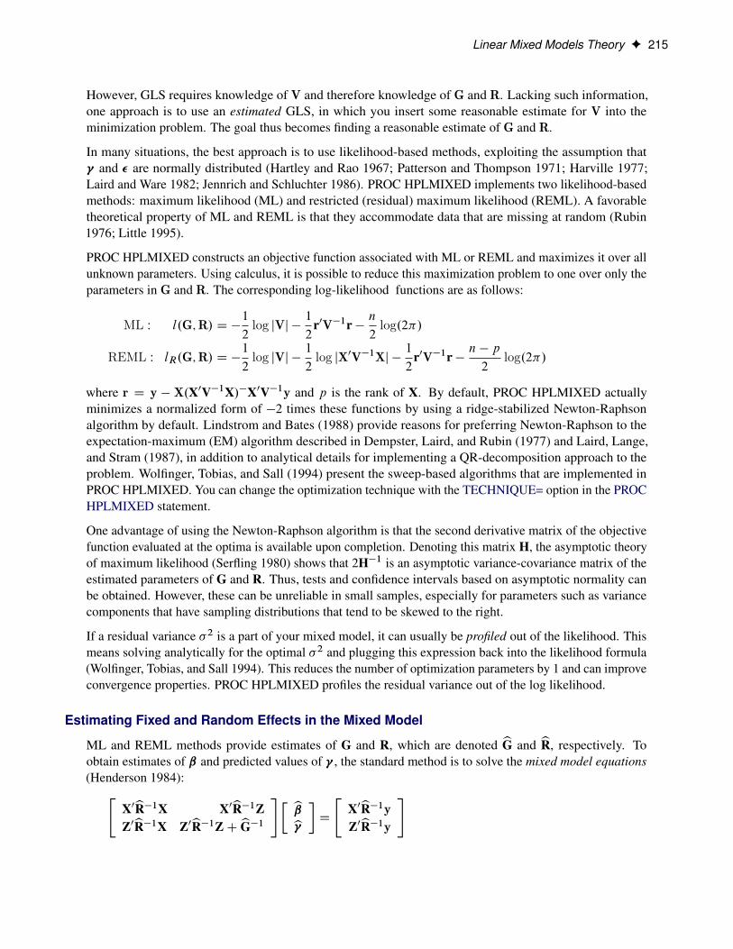
Linear Mixed Models Theory F 215
However, GLS requires knowledge of V and therefore knowledge of G and R. Lacking such information,one approach is to use an estimated GLS, in which you insert some reasonable estimate for V into theminimization problem. The goal thus becomes finding a reasonable estimate of G and R.
In many situations, the best approach is to use likelihood-based methods, exploiting the assumption that and � are normally distributed (Hartley and Rao 1967; Patterson and Thompson 1971; Harville 1977;Laird and Ware 1982; Jennrich and Schluchter 1986). PROC HPLMIXED implements two likelihood-basedmethods: maximum likelihood (ML) and restricted (residual) maximum likelihood (REML). A favorabletheoretical property of ML and REML is that they accommodate data that are missing at random (Rubin1976; Little 1995).
PROC HPLMIXED constructs an objective function associated with ML or REML and maximizes it over allunknown parameters. Using calculus, it is possible to reduce this maximization problem to one over only theparameters in G and R. The corresponding log-likelihood functions are as follows:
ML W l.G;R/ D �1
2log jVj �
1
2r0V�1r �
n
2log.2�/
REML W lR.G;R/ D �1
2log jVj �
1
2log jX0V�1Xj �
1
2r0V�1r �
n � p
2log.2�/
where r D y � X.X0V�1X/�X0V�1y and p is the rank of X. By default, PROC HPLMIXED actuallyminimizes a normalized form of �2 times these functions by using a ridge-stabilized Newton-Raphsonalgorithm by default. Lindstrom and Bates (1988) provide reasons for preferring Newton-Raphson to theexpectation-maximum (EM) algorithm described in Dempster, Laird, and Rubin (1977) and Laird, Lange,and Stram (1987), in addition to analytical details for implementing a QR-decomposition approach to theproblem. Wolfinger, Tobias, and Sall (1994) present the sweep-based algorithms that are implemented inPROC HPLMIXED. You can change the optimization technique with the TECHNIQUE= option in the PROCHPLMIXED statement.
One advantage of using the Newton-Raphson algorithm is that the second derivative matrix of the objectivefunction evaluated at the optima is available upon completion. Denoting this matrix H, the asymptotic theoryof maximum likelihood (Serfling 1980) shows that 2H�1 is an asymptotic variance-covariance matrix of theestimated parameters of G and R. Thus, tests and confidence intervals based on asymptotic normality canbe obtained. However, these can be unreliable in small samples, especially for parameters such as variancecomponents that have sampling distributions that tend to be skewed to the right.
If a residual variance �2 is a part of your mixed model, it can usually be profiled out of the likelihood. Thismeans solving analytically for the optimal �2 and plugging this expression back into the likelihood formula(Wolfinger, Tobias, and Sall 1994). This reduces the number of optimization parameters by 1 and can improveconvergence properties. PROC HPLMIXED profiles the residual variance out of the log likelihood.
Estimating Fixed and Random Effects in the Mixed Model
ML and REML methods provide estimates of G and R, which are denoted bG and bR, respectively. Toobtain estimates of ˇ and predicted values of , the standard method is to solve the mixed model equations(Henderson 1984):"
X0bR�1X X0bR�1ZZ0bR�1X Z0bR�1ZC bG�1
#� bb �D
"X0bR�1yZ0bR�1y
#
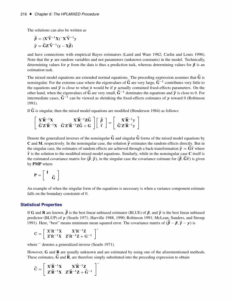
216 F Chapter 6: The HPLMIXED Procedure
The solutions can also be written asbD .X0bV�1X/�X0bV�1yb D bGZ0bV�1.y � Xb/and have connections with empirical Bayes estimators (Laird and Ware 1982; Carlin and Louis 1996).Note that the are random variables and not parameters (unknown constants) in the model. Technically,determining values for from the data is thus a prediction task, whereas determining values for ˇ is anestimation task.
The mixed model equations are extended normal equations. The preceding expression assumes that bG isnonsingular. For the extreme case where the eigenvalues of bG are very large, bG�1 contributes very little tothe equations and b is close to what it would be if actually contained fixed-effects parameters. On theother hand, when the eigenvalues of bG are very small, bG�1 dominates the equations andb is close to 0. Forintermediate cases, bG�1 can be viewed as shrinking the fixed-effects estimates of toward 0 (Robinson1991).
If bG is singular, then the mixed model equations are modified (Henderson 1984) as follows:"X0bR�1X X0bR�1ZbGbG0Z0bR�1X bG0Z0bR�1ZbGCG
#� bb��D
"X0bR�1ybG0Z0bR�1y
#
Denote the generalized inverses of the nonsingular bG and singular bG forms of the mixed model equations byC and M, respectively. In the nonsingular case, the solutionb estimates the random effects directly. But inthe singular case, the estimates of random effects are achieved through a back-transformationb D bGb� whereb� is the solution to the modified mixed model equations. Similarly, while in the nonsingular case C itself isthe estimated covariance matrix for .b;b /, in the singular case the covariance estimate for .b;bGb�/ is givenby PMP where
P D�
I bG�
An example of when the singular form of the equations is necessary is when a variance component estimatefalls on the boundary constraint of 0.
Statistical Properties
If G and R are known, b is the best linear unbiased estimator (BLUE) of ˇ, andb is the best linear unbiasedpredictor (BLUP) of (Searle 1971; Harville 1988, 1990; Robinson 1991; McLean, Sanders, and Stroup1991). Here, “best” means minimum mean squared error. The covariance matrix of .b� ˇ;b � / is
C D�
X0R�1X X0R�1ZZ0R�1X Z0R�1ZCG�1
��where � denotes a generalized inverse (Searle 1971).
However, G and R are usually unknown and are estimated by using one of the aforementioned methods.These estimates, bG and bR, are therefore simply substituted into the preceding expression to obtain
bC D " X0bR�1X X0bR�1ZZ0bR�1X Z0bR�1ZC bG�1
#�
Computational Method F 217
as the approximate variance-covariance matrix of .b�ˇ;b � ). In this case, the BLUE and BLUP acronymsno longer apply, but the word empirical is often added to indicate such an approximation. The appropriateacronyms thus become EBLUE and EBLUP.
McLean and Sanders (1988) show that bC can also be written as
bC D " bC11 bC021bC21 bC22#
where
bC11 D .X0bV�1X/�bC21 D �bGZ0bV�1XbC11bC22 D .Z0bR�1ZC bG�1/�1 �bC21X0bV�1ZbGNote that bC11 is the familiar estimated generalized least squares formula for the variance-covariance matrixof b.
Computational Method
Distributed Computing
Distributed computing refers to the use of multiple autonomous computers that communicate through asecure network. Distributed computing solves computational problems by dividing them into many tasks,each of which is solved by one or more computers. Each computer in this distributed environment is referredto as a node.
You can specify the number of nodes to use with the NODES= option in the PERFORMANCE statement.Specify NODES=0 to force the execution to be done locally (often referred to as single-machine mode).
Multithreading
Threading refers to the organization of computational work into multiple tasks (processing units that canbe scheduled by the operating system). A task is associated with a thread. Multithreading refers to theconcurrent execution of threads. When multithreading is possible, substantial performance gains can berealized compared to sequential (single-threaded) execution.
The number of threads spawned by the HPLMIXED procedure is determined by the number of CPUs on amachine and can be controlled in the following ways:
You can specify the NTHREADS= option in the PERFORMANCE statement to determine the number ofthreads. This specification overrides the system option. Specify NTHREADS=1 to force single-threadedexecution.
The number of threads per machine is displayed in the “Performance Information” table, which is part of thedefault output. The HPLMIXED procedure allocates two threads per CPU.
The tasks multithreaded by the HPLMIXED procedure are primarily defined by dividing the data processedon a single machine among the threads—that is, the HPLMIXED procedure implements multithreadingthrough a data-parallel model. For example, if the input data set has 1,000 observations and you are running
218 F Chapter 6: The HPLMIXED Procedure
with four threads, then 250 observations are associated with each thread. All operations that require access tothe data are then multithreaded. These operations include the following:
• variable levelization
• effect levelization
• formation of the crossproducts matrix
• the log-likelihood computation
In addition, operations on matrices such as sweeps might be multithreaded if the matrices are of sufficientsize to realize performance benefits from managing multiple threads for the particular matrix operation.
Displayed OutputThe following sections describe the output produced by PROC HPLMIXED. The output is organized intovarious tables, which are discussed in the order of their appearance.
Performance Information
The “Performance Information” table is produced by default. It displays information about the executionmode. For single-machine mode, the table displays the number of threads used. For distributed mode, thetable displays the grid mode (symmetric or asymmetric), the number of compute nodes, and the number ofthreads per node.
If you specify the DETAILS option in the PERFORMANCE statement, PROC HPLMIXED also produces a“Timing” table that displays elapsed times (absolute and relative) for the main tasks of the procedure.
Model Information
The “Model Information” table describes the model, some of the variables it involves, and the method used infitting it. The “Model Information” table also has a row labeled Fixed Effects SE Method. This row describesthe method used to compute the approximate standard errors for the fixed-effects parameter estimates andrelated functions of them.
Class Level Information
The “Class Level Information” table lists the levels of every variable specified in the CLASS statement.
Dimensions
The “Dimensions” table lists the sizes of relevant matrices. This table can be useful in determining therequirements for CPU time and memory.
Number of Observations
The “Number of Observations” table shows the number of observations read from the data set and the numberof observations used in fitting the model.

Displayed Output F 219
Optimization Information
The “Optimization Information” table displays important details about the optimization process.
The number of parameters that are updated in the optimization equals the number of parameters in thistable minus the number of equality constraints. The number of constraints is displayed if you fix covarianceparameters with the HOLD= option in the PARMS statement. The HPLMIXED procedure also lists thenumber of upper and lower boundary constraints. PROC HPLMIXED might impose boundary constraintsfor certain parameters, such as variance components and correlation parameters. If you specify the HOLD=option in the PARMS statement, covariance parameters have an upper and lower boundary equal to theparameter value.
Iteration History
The “Iteration History” table describes the optimization of the restricted log likelihood or log likelihood. Thefunction to be minimized (the objective function) is �2l for ML and �2lR for REML; the column name ofthe objective function in the “Iteration History” table is “-2 Log Like” for ML and “-2 Res Log Like” forREML. The minimization is performed by using a ridge-stabilized Newton-Raphson algorithm, and the rowsof this table describe the iterations that this algorithm takes in order to minimize the objective function.
The Evaluations column of the “Iteration History” table tells how many times the objective function isevaluated during each iteration.
The Criterion column of the “Iteration History” table is, by default, a relative Hessian convergence quantitygiven by
g0kH�1k
gkjfkj
where fk is the value of the objective function at iteration k, gk is the gradient (first derivative) of fk , andHk is the Hessian (second derivative) of fk . If Hk is singular, then PROC HPLMIXED uses the followingrelative quantity:
g0kgkjfkj
To prevent division by jfkj, specify the ABSGCONV option in the PROC HPLMIXED statement. To use arelative function or gradient criterion, specify the FCONV or GCONV option, respectively.
The Hessian criterion is considered superior to function and gradient criteria because it measures orthogonalityrather than lack of progress (Bates and Watts 1988). Provided that the initial estimate is feasible and themaximum number of iterations is not exceeded, the Newton-Raphson algorithm is considered to haveconverged when the criterion is less than the tolerance specified with the FCONV or GCONV option inthe PROC HPLMIXED statement. The default tolerance is 1E–8. If convergence is not achieved, PROCHPLMIXED displays the estimates of the parameters at the last iteration.
A convergence criterion that is missing indicates that a boundary constraint has been dropped; it is usuallynot a cause for concern.
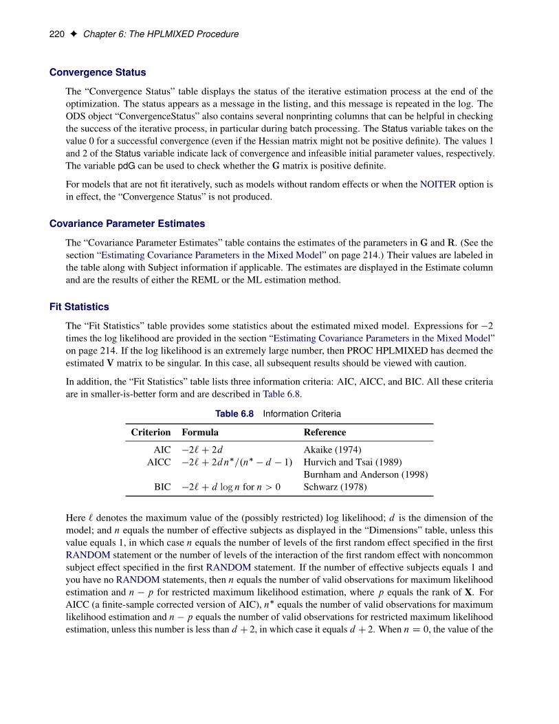
220 F Chapter 6: The HPLMIXED Procedure
Convergence Status
The “Convergence Status” table displays the status of the iterative estimation process at the end of theoptimization. The status appears as a message in the listing, and this message is repeated in the log. TheODS object “ConvergenceStatus” also contains several nonprinting columns that can be helpful in checkingthe success of the iterative process, in particular during batch processing. The Status variable takes on thevalue 0 for a successful convergence (even if the Hessian matrix might not be positive definite). The values 1and 2 of the Status variable indicate lack of convergence and infeasible initial parameter values, respectively.The variable pdG can be used to check whether the G matrix is positive definite.
For models that are not fit iteratively, such as models without random effects or when the NOITER option isin effect, the “Convergence Status” is not produced.
Covariance Parameter Estimates
The “Covariance Parameter Estimates” table contains the estimates of the parameters in G and R. (See thesection “Estimating Covariance Parameters in the Mixed Model” on page 214.) Their values are labeled inthe table along with Subject information if applicable. The estimates are displayed in the Estimate columnand are the results of either the REML or the ML estimation method.
Fit Statistics
The “Fit Statistics” table provides some statistics about the estimated mixed model. Expressions for �2times the log likelihood are provided in the section “Estimating Covariance Parameters in the Mixed Model”on page 214. If the log likelihood is an extremely large number, then PROC HPLMIXED has deemed theestimated V matrix to be singular. In this case, all subsequent results should be viewed with caution.
In addition, the “Fit Statistics” table lists three information criteria: AIC, AICC, and BIC. All these criteriaare in smaller-is-better form and are described in Table 6.8.
Table 6.8 Information Criteria
Criterion Formula Reference
AIC �2`C 2d Akaike (1974)AICC �2`C 2dn�=.n� � d � 1/ Hurvich and Tsai (1989)
Burnham and Anderson (1998)BIC �2`C d log n for n > 0 Schwarz (1978)
Here ` denotes the maximum value of the (possibly restricted) log likelihood; d is the dimension of themodel; and n equals the number of effective subjects as displayed in the “Dimensions” table, unless thisvalue equals 1, in which case n equals the number of levels of the first random effect specified in the firstRANDOM statement or the number of levels of the interaction of the first random effect with noncommonsubject effect specified in the first RANDOM statement. If the number of effective subjects equals 1 andyou have no RANDOM statements, then n equals the number of valid observations for maximum likelihoodestimation and n � p for restricted maximum likelihood estimation, where p equals the rank of X. ForAICC (a finite-sample corrected version of AIC), n� equals the number of valid observations for maximumlikelihood estimation and n � p equals the number of valid observations for restricted maximum likelihoodestimation, unless this number is less than d C 2, in which case it equals d C 2. When n D 0, the value of the
Examples: HPLMIXED Procedure F 221
BIC is �2`. For restricted likelihood estimation, d equals q, the effective number of estimated covarianceparameters. For maximum likelihood estimation, d equals q C p.
Timing Information
If you specify the DETAILS option in the PERFORMANCE statement, the procedure also produces a“Timing” table in which the elapsed time for each main task of the procedure is displayed.
ODS Table NamesEach table created by PROC HPLMIXED has a name associated with it, and you must use this name to referto the table when you use ODS statements. These names are listed in Table 6.9.
Table 6.9 ODS Tables Produced by PROC HPLMIXED
Table Name Description Required Statement / Option
ClassLevels Level information from the CLASSstatement
Default output
ConvergenceStatus Convergence status Default outputCovParms Estimated covariance parameters Default outputDimensions Dimensions of the model Default outputFitStatistics Fit statistics Default outputIterHistory Iteration history Default outputModelInfo Model information Default outputNObs Number of observations read and
usedDefault output
OptInfo Optimization information Default outputParmSearch Parameter search values PARMSPerformanceInfo Information about high-performance
computing environmentDefault output
SolutionF Fixed-effects solution vector MODEL / SSolutionR Random-effects solution vector RANDOM / STiming Timing breakdown by task DETAILS option in the PERFOR-
MANCE statement
Examples: HPLMIXED Procedure
Example 6.1: Computing BLUPs for a Large Number of SubjectsSuppose you are using health measurements on patients treated by each medical center to monitor theperformance of those centers. Different measurements within each patient are correlated, and there is enoughdata to fit the parameters of an unstructured covariance model for this correlation. In fact, long experience
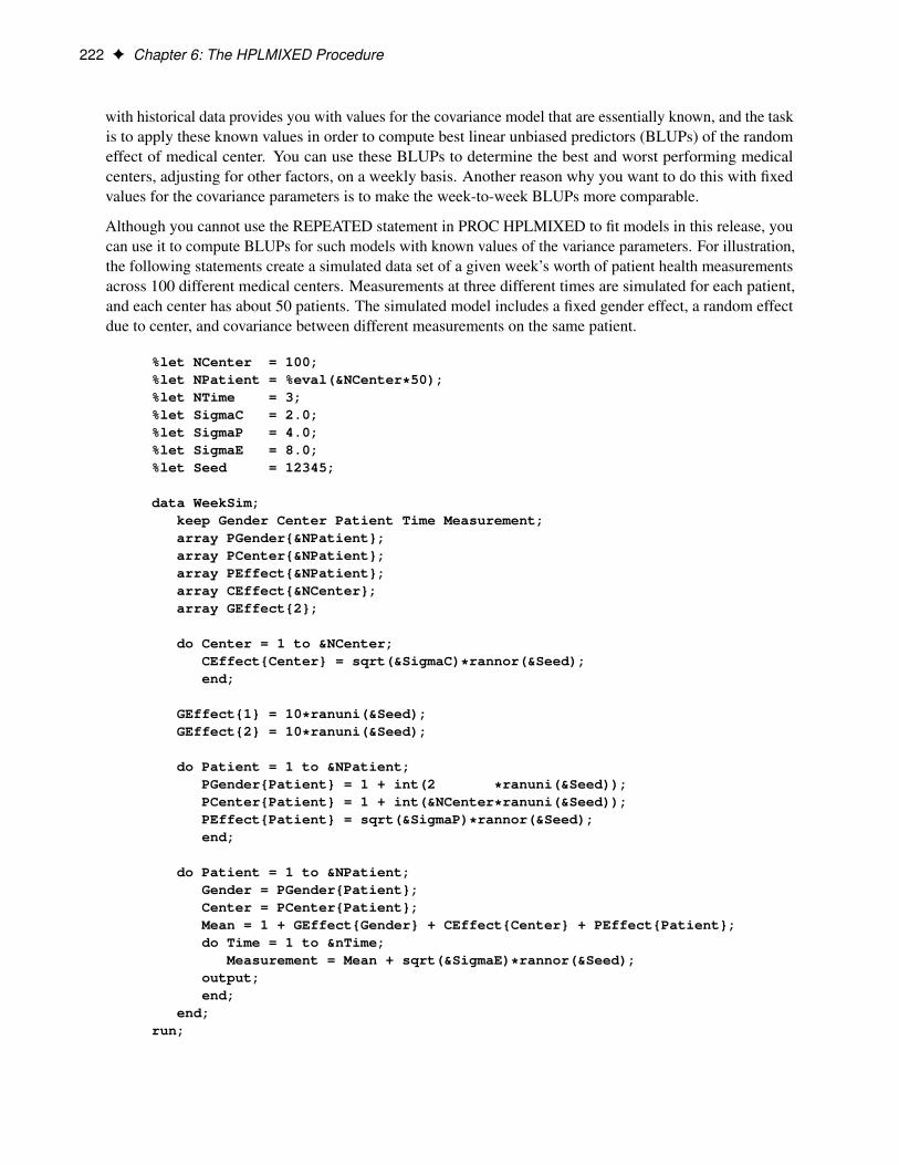
222 F Chapter 6: The HPLMIXED Procedure
with historical data provides you with values for the covariance model that are essentially known, and the taskis to apply these known values in order to compute best linear unbiased predictors (BLUPs) of the randomeffect of medical center. You can use these BLUPs to determine the best and worst performing medicalcenters, adjusting for other factors, on a weekly basis. Another reason why you want to do this with fixedvalues for the covariance parameters is to make the week-to-week BLUPs more comparable.
Although you cannot use the REPEATED statement in PROC HPLMIXED to fit models in this release, youcan use it to compute BLUPs for such models with known values of the variance parameters. For illustration,the following statements create a simulated data set of a given week’s worth of patient health measurementsacross 100 different medical centers. Measurements at three different times are simulated for each patient,and each center has about 50 patients. The simulated model includes a fixed gender effect, a random effectdue to center, and covariance between different measurements on the same patient.
%let NCenter = 100;%let NPatient = %eval(&NCenter*50);%let NTime = 3;%let SigmaC = 2.0;%let SigmaP = 4.0;%let SigmaE = 8.0;%let Seed = 12345;
data WeekSim;keep Gender Center Patient Time Measurement;array PGender{&NPatient};array PCenter{&NPatient};array PEffect{&NPatient};array CEffect{&NCenter};array GEffect{2};
do Center = 1 to &NCenter;CEffect{Center} = sqrt(&SigmaC)*rannor(&Seed);end;
GEffect{1} = 10*ranuni(&Seed);GEffect{2} = 10*ranuni(&Seed);
do Patient = 1 to &NPatient;PGender{Patient} = 1 + int(2 *ranuni(&Seed));PCenter{Patient} = 1 + int(&NCenter*ranuni(&Seed));PEffect{Patient} = sqrt(&SigmaP)*rannor(&Seed);end;
do Patient = 1 to &NPatient;Gender = PGender{Patient};Center = PCenter{Patient};Mean = 1 + GEffect{Gender} + CEffect{Center} + PEffect{Patient};do Time = 1 to &nTime;
Measurement = Mean + sqrt(&SigmaE)*rannor(&Seed);output;end;
end;run;
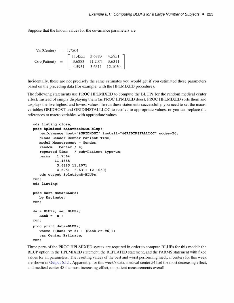
Example 6.1: Computing BLUPs for a Large Number of Subjects F 223
Suppose that the known values for the covariance parameters are
Var(Center) D 1:7564
Cov(Patient) D
24 11:4555 3:6883 4:5951
3:6883 11:2071 3:6311
4:5951 3:6311 12:1050
35
Incidentally, these are not precisely the same estimates you would get if you estimated these parametersbased on the preceding data (for example, with the HPLMIXED procedure).
The following statements use PROC HPLMIXED to compute the BLUPs for the random medical centereffect. Instead of simply displaying them (as PROC HPMIXED does), PROC HPLMIXED sorts them anddisplays the five highest and lowest values. To run these statements successfully, you need to set the macrovariables GRIDHOST and GRIDINSTALLLOC to resolve to appropriate values, or you can replace thereferences to macro variables with appropriate values.
ods listing close;proc hplmixed data=WeekSim blup;
performance host="&GRIDHOST" install="&GRIDINSTALLLOC" nodes=20;class Gender Center Patient Time;model Measurement = Gender;random Center / s;repeated Time / sub=Patient type=un;parms 1.7564
11.45553.6883 11.20714.5951 3.6311 12.1050;
ods output SolutionR=BLUPs;run;ods listing;
proc sort data=BLUPs;by Estimate;
run;
data BLUPs; set BLUPs;Rank = _N_;
run;
proc print data=BLUPs;where ((Rank <= 5) | (Rank >= 96));var Center Estimate;
run;
Three parts of the PROC HPLMIXED syntax are required in order to compute BLUPs for this model: theBLUP option in the HPLMIXED statement, the REPEATED statement, and the PARMS statement with fixedvalues for all parameters. The resulting values of the best and worst performing medical centers for this weekare shown in Output 6.1.1. Apparently, for this week’s data, medical center 54 had the most decreasing effect,and medical center 48 the most increasing effect, on patient measurements overall.
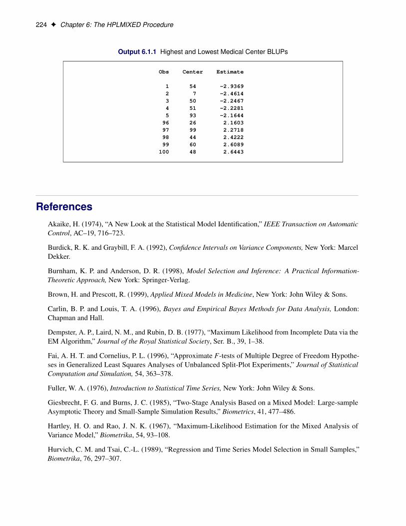
224 F Chapter 6: The HPLMIXED Procedure
Output 6.1.1 Highest and Lowest Medical Center BLUPs
Obs Center Estimate
1 54 -2.93692 7 -2.46143 50 -2.24674 51 -2.22815 93 -2.1644
96 26 2.160397 99 2.271898 44 2.422299 60 2.6089
100 48 2.6443
ReferencesAkaike, H. (1974), “A New Look at the Statistical Model Identification,” IEEE Transaction on AutomaticControl, AC–19, 716–723.
Burdick, R. K. and Graybill, F. A. (1992), Confidence Intervals on Variance Components, New York: MarcelDekker.
Burnham, K. P. and Anderson, D. R. (1998), Model Selection and Inference: A Practical Information-Theoretic Approach, New York: Springer-Verlag.
Brown, H. and Prescott, R. (1999), Applied Mixed Models in Medicine, New York: John Wiley & Sons.
Carlin, B. P. and Louis, T. A. (1996), Bayes and Empirical Bayes Methods for Data Analysis, London:Chapman and Hall.
Dempster, A. P., Laird, N. M., and Rubin, D. B. (1977), “Maximum Likelihood from Incomplete Data via theEM Algorithm,” Journal of the Royal Statistical Society, Ser. B., 39, 1–38.
Fai, A. H. T. and Cornelius, P. L. (1996), “Approximate F-tests of Multiple Degree of Freedom Hypothe-ses in Generalized Least Squares Analyses of Unbalanced Split-Plot Experiments,” Journal of StatisticalComputation and Simulation, 54, 363–378.
Fuller, W. A. (1976), Introduction to Statistical Time Series, New York: John Wiley & Sons.
Giesbrecht, F. G. and Burns, J. C. (1985), “Two-Stage Analysis Based on a Mixed Model: Large-sampleAsymptotic Theory and Small-Sample Simulation Results,” Biometrics, 41, 477–486.
Hartley, H. O. and Rao, J. N. K. (1967), “Maximum-Likelihood Estimation for the Mixed Analysis ofVariance Model,” Biometrika, 54, 93–108.
Hurvich, C. M. and Tsai, C.-L. (1989), “Regression and Time Series Model Selection in Small Samples,”Biometrika, 76, 297–307.
References F 225
Harville, D. A. (1977), “Maximum Likelihood Approaches to Variance Component Estimation and to RelatedProblems,” Journal of the American Statistical Association, 72, 320–338.
Harville, D. A. (1988), “Mixed-Model Methodology: Theoretical Justifications and Future Directions,”Proceedings of the Statistical Computing Section, American Statistical Association, New Orleans, 41–49.
Harville, D. A. (1990), “BLUP (Best Linear Unbiased Prediction), and Beyond,” in Advances in StatisticalMethods for Genetic Improvement of Livestock, Springer-Verlag, 239–276.
Henderson, C. R. (1984), Applications of Linear Models in Animal Breeding, University of Guelph.
Henderson, C. R. (1990), “Statistical Method in Animal Improvement: Historical Overview,” in Advances inStatistical Methods for Genetic Improvement of Livestock, New York: Springer-Verlag, 1–14.
Huynh, H. and Feldt, L. S. (1970), “Conditions Under Which Mean Square Ratios in Repeated MeasurementsDesigns Have Exact F-Distributions,” Journal of the American Statistical Association, 65, 1582–1589.
Jennrich, R. I. and Schluchter, M. D. (1986), “Unbalanced Repeated-Measures Models with StructuredCovariance Matrices,” Biometrics, 42, 805–820.
Kenward, M. G. (1987), “A Method for Comparing Profiles of Repeated Measurements,” Applied Statistics,36, 296–308.
Laird, N. M., Lange, N., and Stram, D. (1987), “Maximum Likelihood Computations with Repeated Measures:Application of the EM Algorithm,” Journal of the American Statistical Association, 82, 97–105.
Laird, N. M. and Ware, J. H. (1982), “Random-Effects Models for Longitudinal Data,” Biometrics, 38,963–974.
Lindstrom, M. J. and Bates, D. M. (1988), “Newton-Raphson and EM Algorithms for Linear Mixed-EffectsModels for Repeated-Measures Data,” Journal of the American Statistical Association, 83, 1014–1022.
Littell, R. C., Milliken, G. A., Stroup, W. W., Wolfinger, R. D., and Schabenberger, O. (2006), SAS for MixedModels, Second Edition, Cary, NC: SAS Institute Inc.
Little, R. J. A. (1995), “Modeling the Drop-Out Mechanism in Repeated-Measures Studies,” Journal of theAmerican Statistical Association, 90, 1112–1121.
Macchiavelli, R. E. and Arnold, S. F. (1994), “Variable Order Ante-dependence Models,” Communications inStatistics–Theory and Methods, 23(9), 2683–2699.
McLean, R. A. and Sanders, W. L. (1988), “Approximating Degrees of Freedom for Standard Errors in MixedLinear Models,” Proceedings of the Statistical Computing Section, American Statistical Association, NewOrleans, 50–59.
McLean, R. A., Sanders, W. L., and Stroup, W. W. (1991), “A Unified Approach to Mixed Linear Models,”The American Statistician, 45, 54–64.
Milliken, G. A. and Johnson, D. E. (1992), Analysis of Messy Data, Volume 1: Designed Experiments, NewYork: Chapman and Hall.
Patel, H. I. (1991), “Analysis of Incomplete Data from a Clinical Trial with Repeated Measurements,”Biometrika, 78, 609–619.

226 F Chapter 6: The HPLMIXED Procedure
Patterson, H. D. and Thompson, R. (1971), “Recovery of Inter-block Information When Block Sizes AreUnequal,” Biometrika, 58, 545–554.
Robinson, G. K. (1991), “That BLUP Is a Good Thing: The Estimation of Random Effects,” StatisticalScience, 6, 15–51.
Rubin, D. B. (1976), “Inference and Missing Data,” Biometrika, 63, 581–592.
Schluchter, M. D. and Elashoff, J. D. (1990), “Small-Sample Adjustments to Tests with Unbalanced RepeatedMeasures Assuming Several Covariance Structures,” Journal of Statistical Computation and Simulation, 37,69–87.
Schwarz, G. (1978), “Estimating the Dimension of a Model,” Annals of Statistics, 6, 461–464.
Searle, S. R. (1971), Linear Models, New York: John Wiley & Sons.
Searle, S. R. (1982), Matrix Algebra Useful for Statisticians, New York: John Wiley & Sons.
Searle, S. R., Casella, G., and McCulloch, C. E. (1992), Variance Components, New York: John Wiley &Sons.
Serfling, R. J. (1980), Approximation Theorems of Mathematical Statistics, New York: John Wiley & Sons.
Snedecor, G. W. and Cochran, W. G. (1980), Statistical Methods, Ames: Iowa State University Press.
Steel, R. G. D., Torrie, J. H., and Dickey D. (1997), Principles and Procedures of Statistics: A BiometricalApproach, Third Edition, New York: McGraw-Hill, Inc.
Verbeke, G. and Molenberghs, G., eds. (1997), Linear Mixed Models in Practice: A SAS-Oriented Approach,New York: Springer.
Verbeke, G. and Molenberghs, G. (2000), Linear Mixed Models for Longitudinal Data, New York: Springer.
Winer, B. J. (1971), Statistical Principles in Experimental Design, Second Edition, New York: McGraw-Hill,Inc.
Wolfinger, R. D. (1996), “Heterogeneous Variance-Covariance Structures for Repeated Measures,” Journalof Agricultural, Biological, and Environmental Statistics, 1, 205–230.
Wolfinger, R. D., Tobias, R. D., and Sall, J. (1994), “Computing Gaussian Likelihoods and Their Derivativesfor General Linear Mixed Models,” SIAM Journal on Scientific Computing, 15(6), 1294–1310.

Chapter 7
The HPNLMOD Procedure
ContentsOverview: HPNLMOD Procedure . . . . . . . . . . . . . . . . . . . . . . . . . . . . . . . 227
PROC HPNLMOD Features . . . . . . . . . . . . . . . . . . . . . . . . . . . . . . . 228PROC HPNLMOD Contrasted with the NLIN and NLMIXED Procedures . . . . . . 228
Getting Started: HPNLMOD Procedure . . . . . . . . . . . . . . . . . . . . . . . . . . . . 229Least Squares Model . . . . . . . . . . . . . . . . . . . . . . . . . . . . . . . . . . . 229Binomial Model . . . . . . . . . . . . . . . . . . . . . . . . . . . . . . . . . . . . . 230
Syntax: HPNLMOD Procedure . . . . . . . . . . . . . . . . . . . . . . . . . . . . . . . . 231PROC HPNLMOD Statement . . . . . . . . . . . . . . . . . . . . . . . . . . . . . . 232BOUNDS Statement . . . . . . . . . . . . . . . . . . . . . . . . . . . . . . . . . . . 237BY Statement . . . . . . . . . . . . . . . . . . . . . . . . . . . . . . . . . . . . . . 237ESTIMATE Statement . . . . . . . . . . . . . . . . . . . . . . . . . . . . . . . . . . 238MODEL Statement . . . . . . . . . . . . . . . . . . . . . . . . . . . . . . . . . . . . 238PARAMETERS Statement . . . . . . . . . . . . . . . . . . . . . . . . . . . . . . . . 239PERFORMANCE Statement . . . . . . . . . . . . . . . . . . . . . . . . . . . . . . 241PREDICT Statement . . . . . . . . . . . . . . . . . . . . . . . . . . . . . . . . . . . 242RESTRICT Statement . . . . . . . . . . . . . . . . . . . . . . . . . . . . . . . . . . 243Programming Statements . . . . . . . . . . . . . . . . . . . . . . . . . . . . . . . . 243
Details: HPNLMOD Procedure . . . . . . . . . . . . . . . . . . . . . . . . . . . . . . . . 245Least Squares Estimation . . . . . . . . . . . . . . . . . . . . . . . . . . . . . . . . 245Built-In Log-Likelihood Functions . . . . . . . . . . . . . . . . . . . . . . . . . . . 246Computational Method . . . . . . . . . . . . . . . . . . . . . . . . . . . . . . . . . . 248Choosing an Optimization Algorithm . . . . . . . . . . . . . . . . . . . . . . . . . . 249Displayed Output . . . . . . . . . . . . . . . . . . . . . . . . . . . . . . . . . . . . . 252ODS Table Names . . . . . . . . . . . . . . . . . . . . . . . . . . . . . . . . . . . . 255
Examples: HPNLMOD Procedure . . . . . . . . . . . . . . . . . . . . . . . . . . . . . . . 256Example 7.1: Segmented Model . . . . . . . . . . . . . . . . . . . . . . . . . . . . 256
References . . . . . . . . . . . . . . . . . . . . . . . . . . . . . . . . . . . . . . . . . . . 260
Overview: HPNLMOD ProcedureThe HPNLMOD procedure is a high-performance procedure that uses either nonlinear least squares ormaximum likelihood to fit nonlinear regression models. PROC HPNLMOD enables you to specify themodel by using SAS programming statements, which give you greater flexibility in modeling the relationship
228 F Chapter 7: The HPNLMOD Procedure
between the response variable and independent (regressor) variables than do SAS procedures that use a morestructured MODEL statement.
PROC HPNLMOD runs in either single-machine mode or distributed mode.
NOTE: Distributed mode requires SAS High-Performance Statistics.
PROC HPNLMOD FeaturesThe HPNLMOD procedure does the following:
• reads input data in parallel and writes output data in parallel when the data source is the appliancedatabase
• is highly multithreaded during all phases of analytic execution
• computes analytical derivatives of user-provided expressions for more robust parameter estimations
• evaluates user-provided expressions and their confidence limits by using the ESTIMATE and PREDICTstatements
• estimates parameters without specifying a particular distribution function by using the least squaresmethod
• estimates parameters by using the maximum likelihood method when either a built-in distributionfunction is specified or a likelihood function is provided
Because the HPNLMOD procedure is a high-performance analytical procedure, it also does the following:
• enables you to run in distributed mode on a cluster of machines that distribute the data and thecomputations
• enables you to run in single-machine mode on the server where SAS is installed
• exploits all the available cores and concurrent threads, regardless of execution mode
For more information, see the section “Processing Modes” on page 6 in Chapter 2, “Shared Concepts andTopics.”
PROC HPNLMOD Contrasted with the NLIN and NLMIXED ProceduresLike the NLIN procedure, the HPNLMOD procedure estimates parameters by using least squares mini-mization for models that are specified by SAS programming statements. However, PROC HPNLMOD canalso perform maximum likelihood estimation when information about the response variable’s distributionis provided. PROC HPNLMOD also has a RESTRICT statement for specifying restrictions on parameterestimates that are more general than those that are available in PROC NLIN. Because the HPNLMOD and
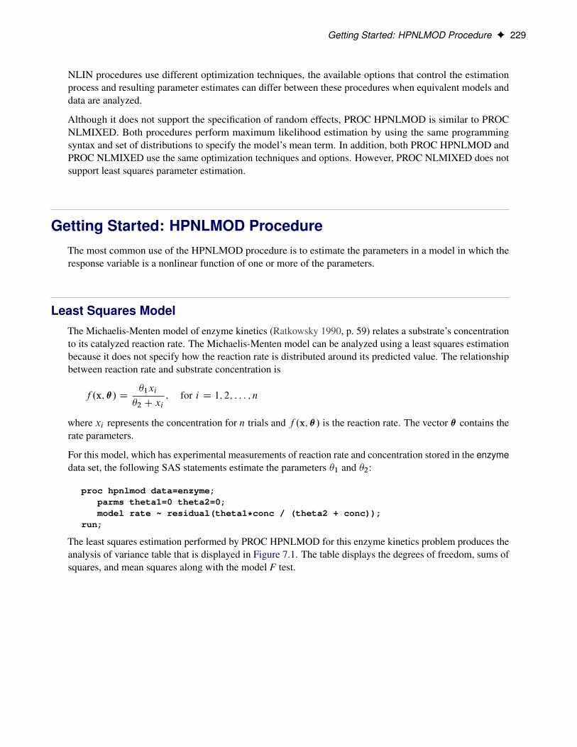
Getting Started: HPNLMOD Procedure F 229
NLIN procedures use different optimization techniques, the available options that control the estimationprocess and resulting parameter estimates can differ between these procedures when equivalent models anddata are analyzed.
Although it does not support the specification of random effects, PROC HPNLMOD is similar to PROCNLMIXED. Both procedures perform maximum likelihood estimation by using the same programmingsyntax and set of distributions to specify the model’s mean term. In addition, both PROC HPNLMOD andPROC NLMIXED use the same optimization techniques and options. However, PROC NLMIXED does notsupport least squares parameter estimation.
Getting Started: HPNLMOD ProcedureThe most common use of the HPNLMOD procedure is to estimate the parameters in a model in which theresponse variable is a nonlinear function of one or more of the parameters.
Least Squares ModelThe Michaelis-Menten model of enzyme kinetics (Ratkowsky 1990, p. 59) relates a substrate’s concentrationto its catalyzed reaction rate. The Michaelis-Menten model can be analyzed using a least squares estimationbecause it does not specify how the reaction rate is distributed around its predicted value. The relationshipbetween reaction rate and substrate concentration is
f .x;�/ D�1xi
�2 C xi; for i D 1; 2; : : : ; n
where xi represents the concentration for n trials and f .x;�/ is the reaction rate. The vector � contains therate parameters.
For this model, which has experimental measurements of reaction rate and concentration stored in the enzymedata set, the following SAS statements estimate the parameters �1 and �2:
proc hpnlmod data=enzyme;parms theta1=0 theta2=0;model rate ~ residual(theta1*conc / (theta2 + conc));
run;
The least squares estimation performed by PROC HPNLMOD for this enzyme kinetics problem produces theanalysis of variance table that is displayed in Figure 7.1. The table displays the degrees of freedom, sums ofsquares, and mean squares along with the model F test.
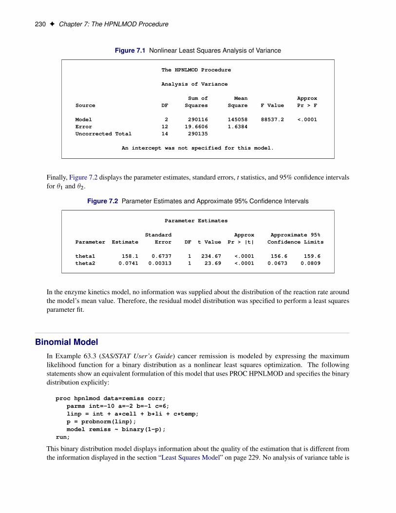
230 F Chapter 7: The HPNLMOD Procedure
Figure 7.1 Nonlinear Least Squares Analysis of Variance
The HPNLMOD Procedure
Analysis of Variance
Sum of Mean ApproxSource DF Squares Square F Value Pr > F
Model 2 290116 145058 88537.2 <.0001Error 12 19.6606 1.6384Uncorrected Total 14 290135
An intercept was not specified for this model.
Finally, Figure 7.2 displays the parameter estimates, standard errors, t statistics, and 95% confidence intervalsfor �1 and �2.
Figure 7.2 Parameter Estimates and Approximate 95% Confidence Intervals
Parameter Estimates
Standard Approx Approximate 95%Parameter Estimate Error DF t Value Pr > |t| Confidence Limits
theta1 158.1 0.6737 1 234.67 <.0001 156.6 159.6theta2 0.0741 0.00313 1 23.69 <.0001 0.0673 0.0809
In the enzyme kinetics model, no information was supplied about the distribution of the reaction rate aroundthe model’s mean value. Therefore, the residual model distribution was specified to perform a least squaresparameter fit.
Binomial ModelIn Example 63.3 (SAS/STAT User’s Guide) cancer remission is modeled by expressing the maximumlikelihood function for a binary distribution as a nonlinear least squares optimization. The followingstatements show an equivalent formulation of this model that uses PROC HPNLMOD and specifies the binarydistribution explicitly:
proc hpnlmod data=remiss corr;parms int=-10 a=-2 b=-1 c=6;linp = int + a*cell + b*li + c*temp;p = probnorm(linp);model remiss ~ binary(1-p);
run;
This binary distribution model displays information about the quality of the estimation that is different fromthe information displayed in the section “Least Squares Model” on page 229. No analysis of variance table is
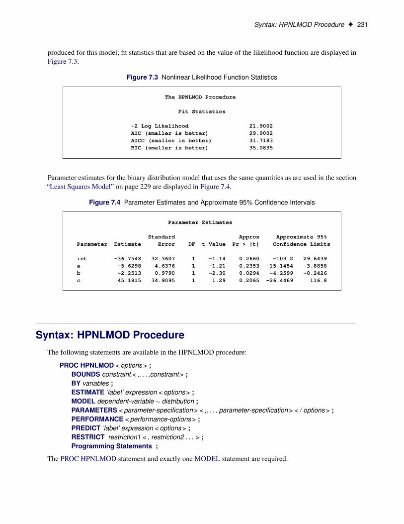
Syntax: HPNLMOD Procedure F 231
produced for this model; fit statistics that are based on the value of the likelihood function are displayed inFigure 7.3.
Figure 7.3 Nonlinear Likelihood Function Statistics
The HPNLMOD Procedure
Fit Statistics
-2 Log Likelihood 21.9002AIC (smaller is better) 29.9002AICC (smaller is better) 31.7183BIC (smaller is better) 35.0835
Parameter estimates for the binary distribution model that uses the same quantities as are used in the section“Least Squares Model” on page 229 are displayed in Figure 7.4.
Figure 7.4 Parameter Estimates and Approximate 95% Confidence Intervals
Parameter Estimates
Standard Approx Approximate 95%Parameter Estimate Error DF t Value Pr > |t| Confidence Limits
int -36.7548 32.3607 1 -1.14 0.2660 -103.2 29.6439a -5.6298 4.6376 1 -1.21 0.2353 -15.1454 3.8858b -2.2513 0.9790 1 -2.30 0.0294 -4.2599 -0.2426c 45.1815 34.9095 1 1.29 0.2065 -26.4469 116.8
Syntax: HPNLMOD ProcedureThe following statements are available in the HPNLMOD procedure:
PROC HPNLMOD < options > ;BOUNDS constraint < ,. . . ,constraint > ;BY variables ;ESTIMATE ’label’ expression < options > ;MODEL dependent-variable � distribution ;PARAMETERS < parameter-specification > < ,. . . , parameter-specification > < / options > ;PERFORMANCE < performance-options > ;PREDICT ’label’ expression < options > ;RESTRICT restriction1 < , restriction2 . . . > ;Programming Statements ;
The PROC HPNLMOD statement and exactly one MODEL statement are required.
232 F Chapter 7: The HPNLMOD Procedure
PROC HPNLMOD StatementPROC HPNLMOD < options > ;
The PROC HPNLMOD statement invokes the procedure. Table 7.1 summarizes important options in thePROC HPNLMOD statement by function. These and other options in the PROC HPNLMOD statement arethen described fully in alphabetical order.
Table 7.1 PROC HPNLMOD Statement Options
Option Description
Basic OptionsDATA= Specifies the input data setOUT= Specifies the output data set
Output OptionsCORR Specifies the correlation matrixCOV Specifies the covariance matrixECORR Specifies the correlation matrix of additional estimatesECOV Specifies the covariance matrix of additional estimatesDF Specifies the default degrees of freedomNOPRINT Suppresses ODS outputNOITPRINT Suppresses output about iterations within the optimization process
Optimization OptionsABSCONV= Tunes an absolute function convergence criterionABSFCONV= Tunes an absolute difference function convergence criterionABSGCONV= Tunes the absolute gradient convergence criterionFCONV= Tunes the relative function convergence criterionGCONV= Tunes the relative gradient convergence criterionMAXITER= Chooses the maximum number of iterations in any optimizationMAXFUNC= Specifies the maximum number of function evaluations in any
optimizationMAXTIME= Specifies the upper limit seconds of CPU time for any optimizationMINITER= Specifies the minimum number of iterations in any optimizationTECHNIQUE= Selects the optimization technique
Tolerance OptionsSINGULAR= Tunes the general singularity criterion
User-Defined Format OptionsFMTLIBXML= Specifies a file reference for a format streamXMLFORMAT= Specifies a file name for a format stream
You can specify the following options in the PROC HPNLMOD statement.

PROC HPNLMOD Statement F 233
ABSCONV=r
ABSTOL=rspecifies an absolute function convergence criterion. For minimization, termination requires f . .k// �r, where is the vector of parameters in the optimization and f .�/ is the objective function. Thedefault value of r is the negative square root of the largest double-precision value, which serves only asa protection against overflow.
ABSFCONV=r < n >
ABSFTOL=r< n >specifies an absolute difference function convergence criterion. For all techniques except the Nelder-Mead simplex (NMSIMP) technique, termination requires a small change of the function value insuccessive iterations:
jf . .k�1// � f . .k//j � r
Here, denotes the vector of parameters that participate in the optimization, and f .�/ is the objectivefunction. The same formula is used for the NMSIMP technique, but .k/ is defined as the vertexthat has the lowest function value, and .k�1/ is defined as the vertex that has the highest functionvalue in the simplex. The default value is r D 0. The optional integer value n specifies the number ofsuccessive iterations for which the criterion must be satisfied before the process can be terminated.
ABSGCONV=r < n >
ABSGTOL=r< n >specifies an absolute gradient convergence criterion. Termination requires the maximum absolutegradient element to be small:
maxjjgj .
.k//j � r
Here, denotes the vector of parameters that participate in the optimization, and gj .�/ is the gradientof the objective function with respect to the j th parameter. This criterion is not used by the NMSIMPtechnique. The default value is r D1E�5. The optional integer value n specifies the number ofsuccessive iterations for which the criterion must be satisfied before the process can be terminated.
ALPHA=˛specifies the level of significance ˛ that is used in the construction of 100.1�˛/% confidence intervals.The value must be strictly between 0 and 1; the default value of ˛ D 0:05 results in 95% intervals. Thisvalue is used as the default confidence level for limits that are computed in the “Parameter Estimates”table and is used in the LOWER and UPPER options in the PREDICT statement.
CORRrequests the approximate correlation matrix for the parameter estimates.
COVrequests the approximate covariance matrix for the parameter estimates.
DATA=SAS-data-setnames the SAS data set to be used by PROC HPNLMOD. The default is the most recently created dataset.
If PROC HPNLMOD executes in distributed mode, the input data are distributed to memory on theappliance nodes and analyzed in parallel, unless the data are already distributed in the appliance
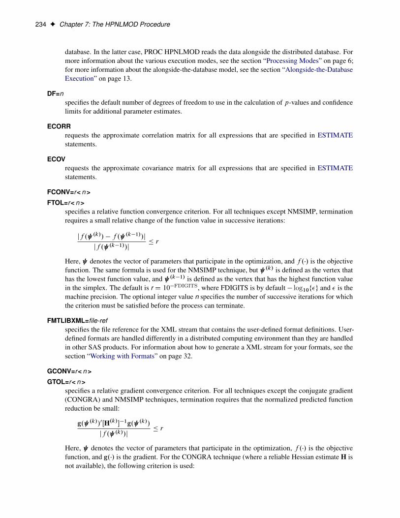
234 F Chapter 7: The HPNLMOD Procedure
database. In the latter case, PROC HPNLMOD reads the data alongside the distributed database. Formore information about the various execution modes, see the section “Processing Modes” on page 6;for more information about the alongside-the-database model, see the section “Alongside-the-DatabaseExecution” on page 13.
DF=nspecifies the default number of degrees of freedom to use in the calculation of p-values and confidencelimits for additional parameter estimates.
ECORRrequests the approximate correlation matrix for all expressions that are specified in ESTIMATEstatements.
ECOVrequests the approximate covariance matrix for all expressions that are specified in ESTIMATEstatements.
FCONV=r< n >
FTOL=r< n >specifies a relative function convergence criterion. For all techniques except NMSIMP, terminationrequires a small relative change of the function value in successive iterations:
jf . .k// � f . .k�1//j
jf . .k�1//j� r
Here, denotes the vector of parameters that participate in the optimization, and f .�/ is the objectivefunction. The same formula is used for the NMSIMP technique, but .k/ is defined as the vertex thathas the lowest function value, and .k�1/ is defined as the vertex that has the highest function valuein the simplex. The default is r D 10�FDIGITS, where FDIGITS is by default � log10f�g and � is themachine precision. The optional integer value n specifies the number of successive iterations for whichthe criterion must be satisfied before the process can terminate.
FMTLIBXML=file-refspecifies the file reference for the XML stream that contains the user-defined format definitions. User-defined formats are handled differently in a distributed computing environment than they are handledin other SAS products. For information about how to generate a XML stream for your formats, see thesection “Working with Formats” on page 32.
GCONV=r< n >
GTOL=r< n >specifies a relative gradient convergence criterion. For all techniques except the conjugate gradient(CONGRA) and NMSIMP techniques, termination requires that the normalized predicted functionreduction be small:
g. .k//0ŒH.k/��1g. .k//jf . .k//j
� r
Here, denotes the vector of parameters that participate in the optimization, f .�/ is the objectivefunction, and g.�/ is the gradient. For the CONGRA technique (where a reliable Hessian estimate H isnot available), the following criterion is used:
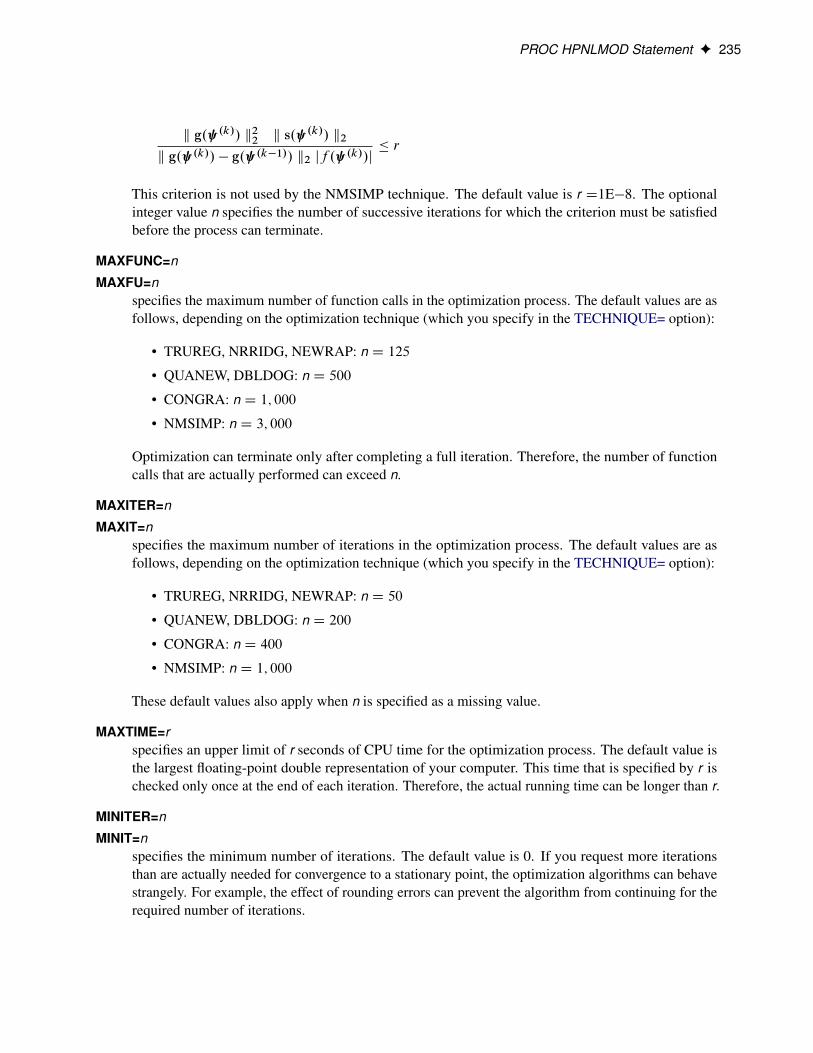
PROC HPNLMOD Statement F 235
k g. .k// k22 k s. .k// k2k g. .k// � g. .k�1// k2 jf . .k//j
� r
This criterion is not used by the NMSIMP technique. The default value is r D1E�8. The optionalinteger value n specifies the number of successive iterations for which the criterion must be satisfiedbefore the process can terminate.
MAXFUNC=n
MAXFU=nspecifies the maximum number of function calls in the optimization process. The default values are asfollows, depending on the optimization technique (which you specify in the TECHNIQUE= option):
• TRUREG, NRRIDG, NEWRAP: n D 125
• QUANEW, DBLDOG: n D 500
• CONGRA: n D 1; 000
• NMSIMP: n D 3; 000
Optimization can terminate only after completing a full iteration. Therefore, the number of functioncalls that are actually performed can exceed n.
MAXITER=n
MAXIT=nspecifies the maximum number of iterations in the optimization process. The default values are asfollows, depending on the optimization technique (which you specify in the TECHNIQUE= option):
• TRUREG, NRRIDG, NEWRAP: n D 50
• QUANEW, DBLDOG: n D 200
• CONGRA: n D 400
• NMSIMP: n D 1; 000
These default values also apply when n is specified as a missing value.
MAXTIME=rspecifies an upper limit of r seconds of CPU time for the optimization process. The default value isthe largest floating-point double representation of your computer. This time that is specified by r ischecked only once at the end of each iteration. Therefore, the actual running time can be longer than r.
MINITER=n
MINIT=nspecifies the minimum number of iterations. The default value is 0. If you request more iterationsthan are actually needed for convergence to a stationary point, the optimization algorithms can behavestrangely. For example, the effect of rounding errors can prevent the algorithm from continuing for therequired number of iterations.
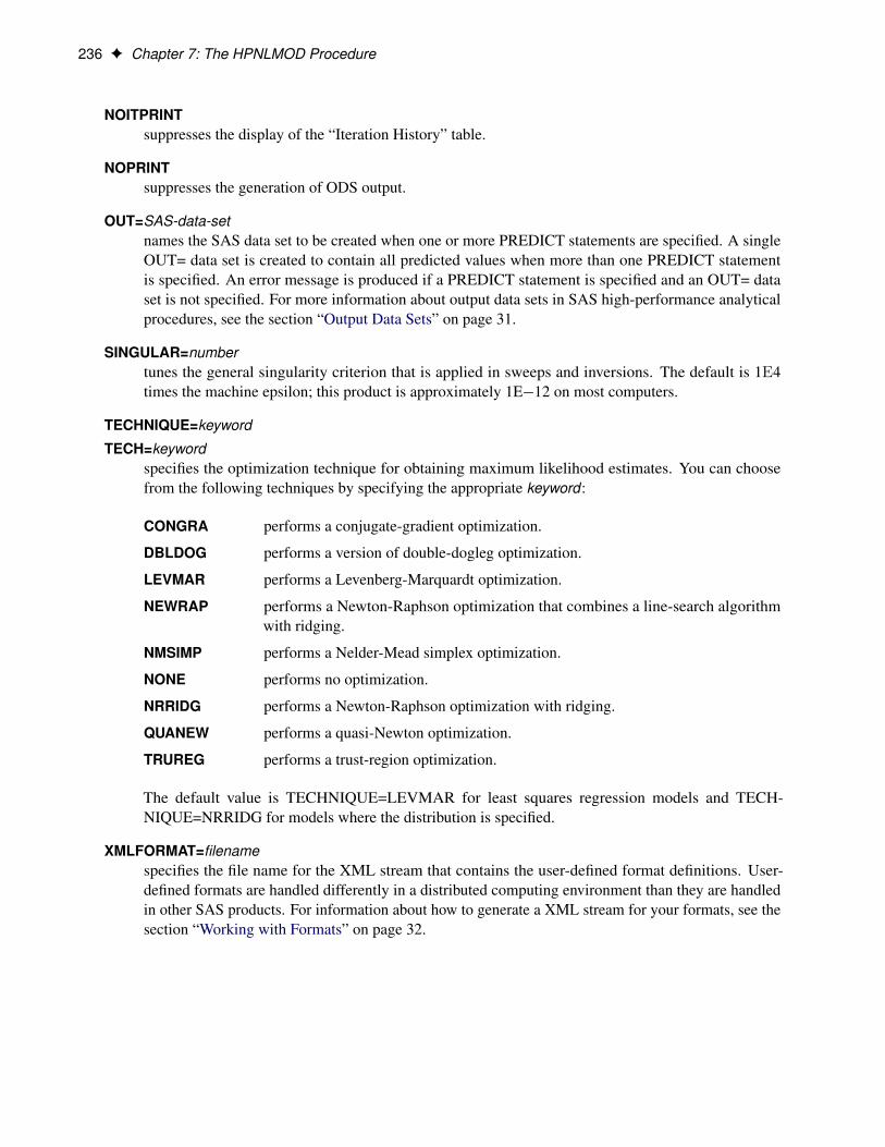
236 F Chapter 7: The HPNLMOD Procedure
NOITPRINTsuppresses the display of the “Iteration History” table.
NOPRINTsuppresses the generation of ODS output.
OUT=SAS-data-setnames the SAS data set to be created when one or more PREDICT statements are specified. A singleOUT= data set is created to contain all predicted values when more than one PREDICT statementis specified. An error message is produced if a PREDICT statement is specified and an OUT= dataset is not specified. For more information about output data sets in SAS high-performance analyticalprocedures, see the section “Output Data Sets” on page 31.
SINGULAR=numbertunes the general singularity criterion that is applied in sweeps and inversions. The default is 1E4times the machine epsilon; this product is approximately 1E�12 on most computers.
TECHNIQUE=keyword
TECH=keywordspecifies the optimization technique for obtaining maximum likelihood estimates. You can choosefrom the following techniques by specifying the appropriate keyword :
CONGRA performs a conjugate-gradient optimization.
DBLDOG performs a version of double-dogleg optimization.
LEVMAR performs a Levenberg-Marquardt optimization.
NEWRAP performs a Newton-Raphson optimization that combines a line-search algorithmwith ridging.
NMSIMP performs a Nelder-Mead simplex optimization.
NONE performs no optimization.
NRRIDG performs a Newton-Raphson optimization with ridging.
QUANEW performs a quasi-Newton optimization.
TRUREG performs a trust-region optimization.
The default value is TECHNIQUE=LEVMAR for least squares regression models and TECH-NIQUE=NRRIDG for models where the distribution is specified.
XMLFORMAT=filenamespecifies the file name for the XML stream that contains the user-defined format definitions. User-defined formats are handled differently in a distributed computing environment than they are handledin other SAS products. For information about how to generate a XML stream for your formats, see thesection “Working with Formats” on page 32.
BOUNDS Statement F 237
BOUNDS StatementBOUNDS constraint < , constraint . . . > ;
where constraint represents
< number operator > parameter-list < operator number >
Boundary constraints are specified in a BOUNDS statement. One- or two-sided boundary constraints areallowed. Elements in a list of boundary constraints are separated by commas. For example:
bounds 0 <= a1-a9 X <= 1, -1 <= c2-c5;bounds b1-b10 y >= 0;
You can specify more than one BOUNDS statement. If you specify more than one lower (or upper) bound forthe same parameter, the maximum (or minimum) of these is taken.
If the maximum lj of all lower bounds is larger than the minimum of all upper bounds uj for the sameparameter �j , the boundary constraint is replaced by �j WD lj WD min.uj /, which is defined by the minimumof all upper bounds specified for �j .
BY StatementBY variables ;
You can specify a BY statement in PROC HPNLMOD to obtain separate analyses of observations in groupsthat are defined by the BY variables. When a BY statement appears, PROC HPNLMOD expects the inputdata set to be sorted in order of the BY variables. If you specify more than one BY statement, only the lastone specified is used.
If your input data set is not sorted in ascending order, use one of the following alternatives:
• Sort the data by using the SORT procedure and a similar BY statement.
• Specify the NOTSORTED or DESCENDING option in the BY statement for the HPNLMOD procedure.The NOTSORTED option does not mean that the data are unsorted but rather that the data are arrangedin groups (according to values of the BY variables) and that these groups are not necessarily inalphabetical or increasing numeric order.
• Create an index on the BY variables by using the DATASETS procedure (in Base SAS software).
BY statement processing is not supported when the HPNLMOD procedure runs alongside the database oralongside the Hadoop distributed file system (HDFS). These modes are used if the input data are stored in adatabase or HDFS and the grid host is the appliance that houses the data.
For more information about BY-group processing, see SAS Language Reference: Concepts. For moreinformation about the DATASETS procedure, see Base SAS Procedures Guide.
238 F Chapter 7: The HPNLMOD Procedure
ESTIMATE StatementESTIMATE ’label’ expression < options > ;
The ESTIMATE statement enables you to compute an additional estimate that is a function of the parametervalues. You must provide a quoted string to identify the estimate and then provide a valid SAS expression.Multiple ESTIMATE statements are permitted, and results from all ESTIMATE statements are listed in acommon table. PROC HPNLMOD computes approximate standard errors for the estimates by using the deltamethod (Billingsley 1986). It uses these standard errors to compute corresponding t statistics, p-values, andconfidence limits.
The ECOV option in the PROC HPNLMOD statement produces a table that contains the approximatecovariance matrix of all the additional estimates you specify. The ECORR option produces the correspondingcorrelation matrix.
You can specify the following options in the ESTIMATE statement:
ALPHA=˛specifies the alpha level to be used to compute confidence limits. The default value corresponds to theALPHA= option in the PROC HPNLMOD statement.
DF=dspecifies the degrees of freedom to be used to compute p-values and confidence limits. The defaultvalue corresponds to the DF= option in the PROC HPNLMOD statement.
MODEL StatementMODEL dependent-variable � distribution ;
The MODEL statement is the mechanism for either using a distribution specification to specify the distributionof the data or using the RESIDUAL distribution to specify a predicted value. You must specify a singledependent variable from the input data set, a tilde (�), and then a distribution along with its parameters. Youcan specify the following values for distribution:
RESIDUAL.m/ or LS.m/ specifies no particular distribution. Instead the sum of squares of the differencesbetween m and the dependent variable is minimized.
NORMAL.m; v/ specifies a normal (Gaussian) distribution that has mean m and variance v.
BINARY.p/ specifies a binary (Bernoulli) distribution that has probability p.
BINOMIAL.n; p/ specifies a binomial distribution that has count n and probability p.
GAMMA.a; b/ specifies a gamma distribution that has shape a and scale b.
NEGBIN.n; p/ specifies a negative binomial distribution that has count n and probability p.
POISSON.m/ specifies a Poisson distribution that has mean m.
GENERAL.ll/ specifies a general log-likelihood function that you construct by using SAS programmingstatements.

PARAMETERS Statement F 239
The MODEL statement must follow any SAS programming statements that you specify for computingparameters of the preceding distributions. For information about the built-in log-likelihood functions, see thesection “Built-In Log-Likelihood Functions” on page 246 .
PARAMETERS StatementPARAMETERS < parameter-specification > < ,. . . , parameter-specification > < / options > ;
PARMS < parameter-specification > < ,. . . , parameter-specification > < / options > ;
The purpose of the PARAMETERS statement is to provide starting values for the HPNLMOD procedure.You can provide values that define a single point in the parameter space or that define a set of points. For moreinformation about parameter-specification, see the section “Assigning Starting Values by Using ParameterSpecification” on page 240.
You can specify the following options in the PARAMETERS statement after the slash (/).
BEST=i > 0
specifies the maximum number of parameter grid points and the corresponding objective functionvalues to display in the “Parameters” table. If you specify this option, the parameter grid points arelisted in ascending order of objective function value. By default, all parameter grid points are displayed.
PDATA=SAS-data-set
DATA=SAS-data-setspecifies the data set that provides parameter starting values.
START=value
DEFSTART=valuespecifies a default starting value for all parameters.
There are four methods available for providing starting values to the optimization process. In descendingorder of precedence, the methods are as follows:
1. Specify values directly in the PARAMETERS statement.
2. Specify values in the PDATA= data set option.
3. Specify a single value for all parameters by using the START= option.
4. Use the default value 1.0.
The names that are assigned to parameters must be valid SAS names and must not coincide with names ofvariables in the input data set (see the DATA= option in the PROC HPNLMOD statement). Parameters thatare assigned starting values through the PARAMETERS statement can be omitted from the estimation if theexpression in the MODEL statement does not depend on them.
240 F Chapter 7: The HPNLMOD Procedure
Assigning Starting Values by Using Parameter Specification
A parameter-specification has the following general form, where name identifies the parameter and value-listprovides the set of starting values for the parameter:
name = value-list
Often the value-list contains only a single value, but more general and flexible list specifications such as thefollowing are possible:
m a single value
m1, m2, . . . , mn several values
m TO n a sequence in which m equals the starting value, n equals the ending value, and theincrement equals 1
m TO n BY i a sequence in which m equals the starting value, n equals the ending value, and theincrement is i
m1, m2 TO m3 mixed values and sequences
When you specify more than one value for a parameter, PROC HPNLMOD sorts the values in ascendingsequence and removes duplicate values from the parameter list before forming the grid for the parametersearch. If you specify several values for each parameter, PROC HPNLMOD evaluates the model at eachpoint on the grid. The iterations then commence from the point on the grid that yields the smallest objectivefunction value.
For example, the following PARAMETERS statement specifies five parameters and sets their possible startingvalues as shown in the following table:
parms b0 = 0b1 = 4 to 8b2 = 0 to .6 by .2b3 = 1, 10, 100b4 = 0, .5, 1 to 4;
Possible Starting Values
B0 B1 B2 B3 B4
0 4 0.0 1 0.05 0.2 10 0.56 0.4 100 1.07 0.6 2.08 3.0
4.0
The objective function values are calculated for each of the 1� 5� 4� 3� 6 D 360 combinations of possiblestarting values. Each grid point’s objective function value is computed by using the execution mode that isspecified in the PERFORMANCE statement.
If you specify a starting value by using a parameter-specification, any starting values that are provided for thisparameter through the PDATA= data set are ignored. The parameter-specification overrides the informationin the PDATA= data set.
PERFORMANCE Statement F 241
Assigning Starting Values from a SAS Data Set
The PDATA= option in the PARAMETERS statement enables you to assign starting values for parameters byusing a SAS data set. The data set must contain at least two variables: a character variable named Parameteror Parm that identifies the parameter, and a numeric variable named Estimate or Est that contains the startingvalues. For example, the PDATA= option enables you to use the contents of the “ParameterEstimates” tablefrom one PROC HPNLMOD run to supply starting values for a subsequent run, as follows:
proc hpnlmod data=d(obs=30);parameters alpha=100 beta=3 gamma=4;Switch = 1/(1+gamma*exp(beta*log(dose)));model y ~ residual(alpha*Switch);ods output ParameterEstimates=pest;
run;
proc hpnlmod data=d;parameters / pdata=pest;Switch = 1/(1+gamma*exp(beta*log(dose)));model y ~ residual(alpha*Switch);
run;
You can specify multiple values for a parameter in the PDATA= data set, and the parameters can appear in anyorder. The starting values are collected by parameter and arranged in ascending order, and duplicate valuesare removed. The parameter names in the PDATA= data set are not case sensitive. For example, the followingDATA step defines starting values for three parameters and a starting grid with 1 � 3 � 1 D 3 points:
data test;input Parameter $ Estimate;datalines;
alpha 100BETA 4beta 4.1
beta 4.2beta 4.1gamma 30
;
PERFORMANCE StatementPERFORMANCE < performance-options > ;
The PERFORMANCE statement defines performance parameters for multithreaded and distributed comput-ing, passes variables that describe the distributed computing environment, and requests detailed results aboutthe performance characteristics of the procedure.
You can also use the PERFORMANCE statement to control whether PROC HPNLMOD executes in single-machine mode or distributed mode.
The PERFORMANCE statement is documented further in the section “PERFORMANCE Statement” onpage 34 of Chapter 2, “Shared Concepts and Topics.”
242 F Chapter 7: The HPNLMOD Procedure
PREDICT StatementPREDICT ’label’ expression < options > ;
PREDICT ’label’ MEAN < options > ;
The PREDICT statement enables you to construct predictions of an expression across all of the observationsin the input data set. Multiple PREDICT statements are permitted. You must provide a quoted string toidentify the predicted expression and then provide the predicted value. You can specify the predicted valueeither by using a SAS programming expression that involves the input data set variables and parameters or byusing the keyword MEAN. If you specify the keyword MEAN, the predicted mean value for the distributionspecified in the MODEL statement is used. Predicted values are computed using the final parameter estimates.Standard errors of prediction are computed using the delta method (Billingsley 1986; Cox 1998). Results forall PREDICT statements are placed in the output data set that you specify in the OUT= option in the PROCHPNLMOD statement. For more information, see the section “Output Data Sets” on page 31.
The following options are available in the PREDICT statement.
ALPHA=˛specifies the alpha level to be used to compute confidence limits. The default value corresponds to theALPHA= option in the PROC HPNLMOD statement.
DF=dspecifies the degrees of freedom to be used to compute confidence limits. The default value correspondsto the DF= option in the PROC HPNLMOD statement.
LOWER=namespecifies a variable that contains the lower confidence limit of the predicted value.
PRED=namespecifies a variable that contains the predicted value.
PROBT=namespecifies a variable that contains the p-value of the predicted value.
STDERR=namespecifies a variable that contains the standard error of the predicted value.
TVALUE=namespecifies a variable that contains the t statistic for the predicted value.
UPPER=namespecifies a variable that contains the upper confidence limit of the predicted value.
RESTRICT Statement F 243
RESTRICT StatementRESTRICT restriction1 < , restriction2 . . . > ;
The RESTRICT statement imposes linear restrictions on the model’s parameters estimates. You can specifyany number of RESTRICT statements.
Each restriction is written as an expression, optionally followed by an equality operator (=) or an inequalityoperator (<, >, <=, >=), followed by a second expression as follows:
expression < operator expression >
The operator can be =, <, >, <= , or >=. The operator and second expression are optional. When they areomitted, the operator defaults to = and the second expression defaults to the value 0.
Restriction expressions can be composed of parameter names, arithmetic operators, functions, and constants.Comparison operators (such as = or <) and logical operators (such as &) cannot be used in RESTRICTstatement expressions. Parameters that are named in restriction expressions must be among the parametersthat are estimated by the model. Restriction expressions cannot refer to other variables that are defined in theprogram or the DATA= data set. The restriction expressions must be linear functions of the parameters.
The following example illustrates how to use the RESTRICT statement to impose a linear constraint onparameters:
proc hpnlmod;parms alpha beta;f = (x/alpha + beta)**2model y ~ residual(f);restrict beta < 2*(alpha + constant('pi'));
run;
The preceding RESTRICT statement represents the following model constraint:
ˇ < 2.˛ C �/
Programming StatementsProgramming statements define the arguments of the MODEL, ESTIMATE, and PREDICT statements inPROC HPNLMOD. Most of the programming statements that can be used in the SAS DATA step can alsobe used in the HPNLMOD procedure. See SAS Language Reference: Concepts for a description of SASprogramming statements. The following are valid programming statements:

244 F Chapter 7: The HPNLMOD Procedure
ABORT;CALL name [ ( expression [, expression . . . ] ) ];DELETE;DO[variable = expression
[TO expression] [BY expression][, expression [ TO expression] [ BY expression ] . . . ]][ WHILE expression ] [ UNTIL expression ] ;
END;GOTO statement_label;IF expression;IF expression THEN program_statement;
ELSE program_statement;variable = expression;variable + expression;LINK statement_label;PUT [variable] [=] [...];RETURN;SELECT[(expression)];STOP;SUBSTR( variable, index, length )= expression;WHEN (expression) program_statement;
OTHERWISE program_statement;
For the most part, the SAS programming statements work the same as they do in the SAS DATA step, asdocumented in SAS Language Reference: Concepts. However, they differ as follows:
• The ABORT statement does not allow any arguments.
• The DO statement does not allow a character index variable. Thus, the first of the following statementsis supported, but the second is not:
do i = 1,2,3;
do i = 'A','B','C';
• In contrast to other procedures that share PROC HPNLMOD’s programming syntax, PROCHPNLMOD does not support the LAG function. Because observations are not processed sequentiallywhen high-performance analytical procedures perform the parameter optimization, informaton forcomputing lagged values is not available.
• The PUT statement, used mostly for program debugging in PROC HPNLMOD, supports only some ofthe features of the DATA step PUT statement, and it has some new features that the DATA step PUTstatement does not have:
– The PROC HPNLMOD PUT statement does not support line pointers, factored lists, iterationfactors, overprinting, _INFILE_, the colon (:) format modifier, or “$”.
– The PROC HPNLMOD PUT statement supports expressions, but the expression must be enclosedin parentheses. For example, the following statement displays the square root of x:

Details: HPNLMOD Procedure F 245
put (sqrt(x));
– The PROC HPNLMOD PUT statement supports the item _PDV_, which displays a formattedlisting of all variables in the program. For example, the following statement displays a muchmore readable listing of the variables than the _ALL_ print item:
put _pdv_;
• The WHEN and OTHERWISE statements enable you to specify more than one programming statement.That is, DO/END groups are not necessary for multiple WHEN statements. For example, the followingsyntax is valid:
select;when (exp1) stmt1;
stmt2;when (exp2) stmt3;
stmt4;end;
When you code your programming statements, avoid defining variables that begin with an underscore (_)because they might conflict with internal variables that are created by PROC HPNLMOD. The MODELstatement must come after any SAS programming statements that define or modify terms that are used tospecify the model.
Details: HPNLMOD Procedure
Least Squares EstimationModels that are estimated by PROC HPNLMOD can be represented by using the equations
Y D f.ˇI z1; � � � ; zk/C �EŒ�� D 0
VarŒ�� D �2I
where
Y is the .n � 1/ vector of observed responses
f is the nonlinear prediction function of parameters and regressor variables
ˇ is the vector of model parameters to be estimated
z1; � � � ; zk are the .n � 1/ vectors for each of the k regressor variables
� is the .n � 1/ vector of residuals
�2 is the variance of the residuals
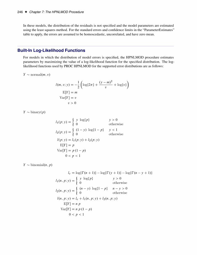
246 F Chapter 7: The HPNLMOD Procedure
In these models, the distribution of the residuals is not specified and the model parameters are estimatedusing the least squares method. For the standard errors and confidence limits in the “ParameterEstimates”table to apply, the errors are assumed to be homoscedastic, uncorrelated, and have zero mean.
Built-In Log-Likelihood FunctionsFor models in which the distribution of model errors is specified, the HPNLMOD procedure estimatesparameters by maximizing the value of a log-likelihood function for the specified distribution. The log-likelihood functions used by PROC HPNLMOD for the supported error distributions are as follows:
Y � normal.m; v/
l.m; vIy/ D �1
2
�logf2�g C
.y �m/2
vC logfvg
�EŒY � D m
VarŒY � D vv > 0
Y � binary.p/
l1.pIy/ D
�y logfpg y > 0
0 otherwise
l2.pIy/ D
�.1 � y/ logf1 � pg y < 1
0 otherwise
l.pIy/ D l1.pIy/C l2.pIy/
EŒY � D pVarŒY � D p .1 � p/
0 < p < 1
Y � binomial.n; p/
lc D logf�.nC 1/g � logf�.y C 1/g � logf�.n � y C 1/g
l1.n; pIy/ D
�y logfpg y > 0
0 otherwise
l2.n; pIy/ D
�.n � y/ logf1 � pg n � y > 0
0 otherwise
l.n; pIy/ D lc C l1.n; pIy/C l2.n; pIy/
EŒY � D npVarŒY � D np .1 � p/
0 < p < 1
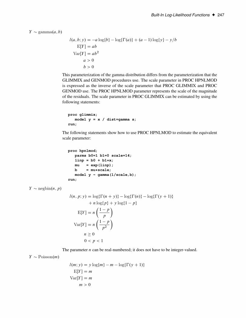
Built-In Log-Likelihood Functions F 247
Y � gamma.a; b/
l.a; bIy/ D �a logfbg � logf�.a/g C .a � 1/ logfyg � y=bEŒY � D ab
VarŒY � D ab2
a > 0
b > 0
This parameterization of the gamma distribution differs from the parameterization that theGLIMMIX and GENMOD procedures use. The scale parameter in PROC HPNLMODis expressed as the inverse of the scale parameter that PROC GLIMMIX and PROCGENMOD use. The PROC HPNLMOD parameter represents the scale of the magnitudeof the residuals. The scale parameter in PROC GLIMMIX can be estimated by using thefollowing statements:
proc glimmix;model y = x / dist=gamma s;
run;
The following statements show how to use PROC HPNLMOD to estimate the equivalentscale parameter:
proc hpnlmod;parms b0=1 b1=0 scale=14;linp = b0 + b1*x;mu = exp(linp);b = mu*scale;model y ~ gamma(1/scale,b);
run;
Y � negbin.n; p/
l.n; pIy/ D logf�.nC y/g � logf�.n/g � logf�.y C 1/gC n logfpg C y logf1 � pg
EŒY � D n�1 � p
p
�VarŒY � D n
�1 � p
p2
�n � 0
0 < p < 1
The parameter n can be real-numbered; it does not have to be integer-valued.
Y � Poisson.m/
l.mIy/ D y logfmg �m � logf�.y C 1/gEŒY � D m
VarŒY � D mm > 0

248 F Chapter 7: The HPNLMOD Procedure
Computational Method
Multithreading
Threading refers to the organization of computational work into multiple tasks (processing units that canbe scheduled by the operating system). A task is associated with a thread. Multithreading refers to theconcurrent execution of threads. When multithreading is possible, substantial performance gains can berealized compared to sequential (single-threaded) execution.
The number of threads that the HPNLMOD procedure spawns is determined by the number of CPUs on amachine and can be controlled in the following ways:
• You can specify the CPU count by using the CPUCOUNT= SAS system option. For example, if youspecify the following statement, the HPNLMOD procedure determines threading as if it executed on asystem that has four CPUs, regardless of the actual CPU count:
options cpucount=4;
• You can specify the NTHREADS= option in the PERFORMANCE statement to determine the numberof threads. This specification overrides the CPUCOUNT= system option. Specify NTHREADS=1 toforce single-threaded execution.
The number of threads per machine is displayed in the “Performance Information” table, which is part of thedefault output. The HPNLMOD procedure allocates one thread per CPU.
The HPNLMOD procedure divides the data that are processed on a single machine among the threads—thatis, the HPNLMOD procedure implements multithreading by parallelizing computations across the data. Forexample, if the input data set has 1; 000 observations and PROC HPNLMOD is running with four threads,then 250 observations are associated with each thread. All operations that require access to the data are thenmultithreaded. These operations include the following:
• calculation of objective function values for the initial parameter grid
• objective function calculation
• gradient calculation
• Hessian calculation
• scoring of observations
In addition, operations on matrices such as sweeps might be multithreaded, provided that the matrices areof sufficient size to realize performance benefits from managing multiple threads for the particular matrixoperation.
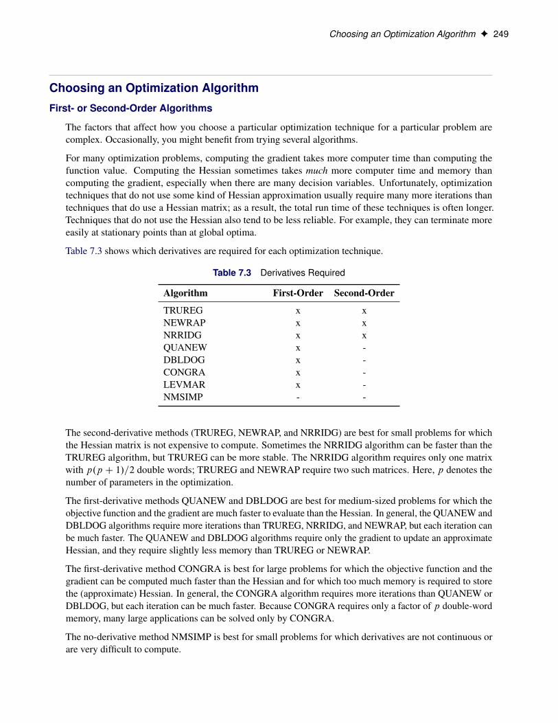
Choosing an Optimization Algorithm F 249
Choosing an Optimization Algorithm
First- or Second-Order Algorithms
The factors that affect how you choose a particular optimization technique for a particular problem arecomplex. Occasionally, you might benefit from trying several algorithms.
For many optimization problems, computing the gradient takes more computer time than computing thefunction value. Computing the Hessian sometimes takes much more computer time and memory thancomputing the gradient, especially when there are many decision variables. Unfortunately, optimizationtechniques that do not use some kind of Hessian approximation usually require many more iterations thantechniques that do use a Hessian matrix; as a result, the total run time of these techniques is often longer.Techniques that do not use the Hessian also tend to be less reliable. For example, they can terminate moreeasily at stationary points than at global optima.
Table 7.3 shows which derivatives are required for each optimization technique.
Table 7.3 Derivatives Required
Algorithm First-Order Second-Order
TRUREG x xNEWRAP x xNRRIDG x xQUANEW x -DBLDOG x -CONGRA x -LEVMAR x -NMSIMP - -
The second-derivative methods (TRUREG, NEWRAP, and NRRIDG) are best for small problems for whichthe Hessian matrix is not expensive to compute. Sometimes the NRRIDG algorithm can be faster than theTRUREG algorithm, but TRUREG can be more stable. The NRRIDG algorithm requires only one matrixwith p.p C 1/=2 double words; TRUREG and NEWRAP require two such matrices. Here, p denotes thenumber of parameters in the optimization.
The first-derivative methods QUANEW and DBLDOG are best for medium-sized problems for which theobjective function and the gradient are much faster to evaluate than the Hessian. In general, the QUANEW andDBLDOG algorithms require more iterations than TRUREG, NRRIDG, and NEWRAP, but each iteration canbe much faster. The QUANEW and DBLDOG algorithms require only the gradient to update an approximateHessian, and they require slightly less memory than TRUREG or NEWRAP.
The first-derivative method CONGRA is best for large problems for which the objective function and thegradient can be computed much faster than the Hessian and for which too much memory is required to storethe (approximate) Hessian. In general, the CONGRA algorithm requires more iterations than QUANEW orDBLDOG, but each iteration can be much faster. Because CONGRA requires only a factor of p double-wordmemory, many large applications can be solved only by CONGRA.
The no-derivative method NMSIMP is best for small problems for which derivatives are not continuous orare very difficult to compute.

250 F Chapter 7: The HPNLMOD Procedure
The LEVMAR method is appropriate only for least squares optimization problems.
Each optimization method uses one or more convergence criteria that determine when it has converged. Analgorithm is considered to have converged when any one of the convergence criteria is satisfied. For example,under the default settings, the QUANEW algorithm converges if ABSGCONV <1E�5, FCONV < 2 � �, orGCONV <1E�8.
By default, the HPNLMOD procedure applies the NRRIDG algorithm because it can take advantage of mutli-threading in Hessian computations and inversions. If the number of parameters becomes large, specifyingTECHNIQUE=QUANEW (which is a first-order method with good overall properties) is recommended.
Algorithm Descriptions
The following subsections provide details about each optimization technique and follow the same order asTable 7.3.
Trust Region Optimization (TRUREG)The trust region method uses the gradient g. .k// and the Hessian matrix H. .k//; thus, it requires that theobjective function f . / have continuous first- and second-order derivatives inside the feasible region.
The trust region method iteratively optimizes a quadratic approximation to the nonlinear objective functionwithin a hyperelliptic trust region that has radius �. Th radius constrains the step size that corresponds to thequality of the quadratic approximation. The trust region method is implemented based on Dennis, Gay, andWelsch (1981); Gay (1983); Moré and Sorensen (1983).
The trust region method performs well for small- to medium-sized problems, and it does not need manyfunction, gradient, and Hessian calls. However, if the computation of the Hessian matrix is computationallyexpensive, one of the quasi-Newton or conjugate gradient algorithms might be more efficient.
Newton-Raphson Optimization with Line Search (NEWRAP)The NEWRAP technique uses the gradient g. .k// and the Hessian matrix H. .k//; thus, it requires that theobjective function have continuous first- and second-order derivatives inside the feasible region.
If second-order derivatives are computed efficiently and precisely, the NEWRAP method can perform wellfor medium-sized to large problems, and it does not need many function, gradient, and Hessian calls.
This algorithm uses a pure Newton step when the Hessian is positive-definite and when the Newton stepreduces the value of the objective function successfully. Otherwise, a combination of ridging and line searchis performed to compute successful steps. If the Hessian is not positive-definite, a multiple of the identitymatrix is added to the Hessian matrix to make it positive-definite (Eskow and Schnabel 1991).
In each iteration, a line search is performed along the search direction to find an approximate optimum ofthe objective function. The default line-search method uses quadratic interpolation and cubic extrapolation(LIS=2).
Newton-Raphson Ridge Optimization (NRRIDG)The NRRIDG technique uses the gradient g. .k// and the Hessian matrix H. .k//; thus, it requires that theobjective function have continuous first- and second-order derivatives inside the feasible region.
This algorithm uses a pure Newton step when the Hessian is positive-definite and when the Newton stepreduces the value of the objective function successfully. If at least one of these two conditions is not satisfied,a multiple of the identity matrix is added to the Hessian matrix.
Choosing an Optimization Algorithm F 251
The NRRIDG method performs well for small- to medium-sized problems, and it does not require manyfunction, gradient, and Hessian calls. However, if the computation of the Hessian matrix is computationallyexpensive, one of the quasi-Newton or conjugate gradient algorithms might be more efficient.
Because the NRRIDG technique uses an orthogonal decomposition of the approximate Hessian, each iterationof NRRIDG can be slower than an iteration of the NEWRAP technique, which works with a Choleskydecomposition. However, NRRIDG usually requires fewer iterations than NEWRAP.
Quasi-Newton Optimization (QUANEW)The (dual) quasi-Newton method uses the gradient g. .k//, and it does not need to compute second-orderderivatives because they are approximated. It works well for medium-sized to moderately large optimizationproblems, where the objective function and the gradient can be computed much faster than the Hessian.However, in general it requires more iterations than the TRUREG, NEWRAP, and NRRIDG techniques,which compute second-order derivatives. QUANEW is the default optimization algorithm because it providesan appropriate balance between the speed and stability that are required for most nonlinear mixed modelapplications.
The QUANEW technique that is implemented by the HPNLMOD procedure is the dual quasi-Newtonalgorithm, which updates the Cholesky factor of an approximate Hessian.
In each iteration, a line search is performed along the search direction to find an approximate optimum. Theline-search method uses quadratic interpolation and cubic extrapolation to obtain a step size ˛ that satisfiesthe Goldstein conditions (Fletcher 1987). One of the Goldstein conditions can be violated if the feasibleregion defines an upper limit of the step size. Violating the left-side Goldstein condition can affect thepositive-definiteness of the quasi-Newton update. In that case, either the update is skipped or the iterationsare restarted by using an identity matrix, resulting in the steepest descent or ascent search direction.
The QUANEW algorithm uses its own line-search technique.
Double-Dogleg Optimization (DBLDOG)The double-dogleg optimization method combines the ideas of the quasi-Newton and trust region methods.In each iteration, the double-dogleg algorithm computes the step s.k/ as the linear combination of the steepestdescent or ascent search direction s.k/1 and a quasi-Newton search direction s.k/2 :
s.k/ D ˛1s.k/1 C ˛2s
.k/2
The step is requested to remain within a prespecified trust region radius (Fletcher 1987, p. 107). Thus, theDBLDOG subroutine uses the dual quasi-Newton update but does not perform a line search.
The double-dogleg optimization technique works well for medium-sized to moderately large optimizationproblems, where the objective function and the gradient are much faster to compute than the Hessian. Theimplementation is based on Dennis and Mei (1979); Gay (1983), but it is extended for dealing with boundaryand linear constraints. The DBLDOG technique generally requires more iterations than the TRUREG,NEWRAP, and NRRIDG techniques, which require second-order derivatives; however, each of the DBLDOGiterations is computationally cheap. Furthermore, the DBLDOG technique requires only gradient calls forthe update of the Cholesky factor of an approximate Hessian.
Conjugate Gradient Optimization (CONGRA)Second-order derivatives are not required by the CONGRA algorithm and are not even approximated. TheCONGRA algorithm can be expensive in function and gradient calls, but it requires only O.p/ memory
252 F Chapter 7: The HPNLMOD Procedure
for unconstrained optimization. In general, the algorithm must perform many iterations to obtain a precisesolution, but each of the CONGRA iterations is computationally cheap.
The CONGRA algorithm should be used for optimization problems that have large p. For the unconstrainedor boundary-constrained case, the CONGRA algorithm requires only O.p/ bytes of working memory,whereas all other optimization methods require order O.p2/ bytes of working memory. During p successiveiterations, uninterrupted by restarts or changes in the working set, the CONGRA algorithm computes a cycleof p conjugate search directions. In each iteration, a line search is performed along the search directionto find an approximate optimum of the objective function. The default line-search method uses quadraticinterpolation and cubic extrapolation to obtain a step size ˛ that satisfies the Goldstein conditions. One ofthe Goldstein conditions can be violated if the feasible region defines an upper limit for the step size. Otherline-search algorithms can be specified with the LIS= option.
Levenberg-Marquardt Optimization (LEVMAR)The LEVMAR algorithm performs a highly stable optimization; however, for large problems, it consumesmore memory and takes longer than the other techniques. The Levenberg-Marquardt optimization techniqueis a slightly improved variant of the Moré (1978) implementation.
Nelder-Mead Simplex Optimization (NMSIMP)The Nelder-Mead simplex method does not use any derivatives and does not assume that the objectivefunction has continuous derivatives. The objective function itself needs to be continuous. This technique isquite expensive in the number of function calls, and it might be unable to generate precise results for p � 40.
The original Nelder-Mead simplex algorithm is implemented and extended to boundary constraints. Thisalgorithm does not compute the objective for infeasible points, but it changes the shape of the simplex byadapting to the nonlinearities of the objective function. This adaptation contributes to an increased speed ofconvergence. NMSIMP uses a special termination criterion.
Displayed OutputThe following sections describe the output that PROC HPNLMOD produces by default. The output isorganized into various tables, which are discussed in the order of their appearance.
Performance Information
The “Performance Information” table is produced by default. It displays information about the executionmode. For single-machine mode, the table displays the number of threads used. For distributed mode, thetable displays the grid mode (symmetric or asymmetric), the number of compute nodes, and the number ofthreads per node.
If you specify the DETAILS option in the PERFORMANCE statement, the procedure also produces a“Timing” table in which elapsed times (absolute and relative) for the main tasks of the procedure aredisplayed.
Specifications
The “Specifications” table displays basic information about the model such as the data source, the dependentvariable, the distribution being modeled, and the optimization technique.
Displayed Output F 253
Number of Observations
The “Number of Observations” table displays the number of observations that are read from the input dataset and the number of observations that are used in the analysis.
Dimensions
The “Dimensions” table displays the number of parameters that are estimated in the model and the number ofupper and lower bounds that are imposed on the parameters.
Parameters
The “Parameters” table displays the initial values of parameters that are used to start the estimation process.You can limit this information by specifying the BEST= option in the PARAMETERS statement whenyou specify a large number of initial parameter value combinations. The parameter combinations and theircorresponding objective function values are listed in increasing order of objective function value.
Iteration History
For each iteration of the optimization, the “Iteration History” table displays the number of function evaluations(including gradient and Hessian evaluations), the value of the objective function, the change in the objectivefunction from the previous iteration, and the absolute value of the largest (projected) gradient element.
Convergence Status
The convergence status table is a small ODS table that follows the “Iteration History” table in the defaultoutput. In the listing it appears as a message that identifies whether the optimization succeeded and whichconvergence criterion was met. If the optimization fails, the message indicates the reason for the failure. Ifyou save the convergence status table to an output data set, a numeric Status variable is added that enablesyou to programmatically assess convergence. The values of the Status variable encode the following:
0 Convergence was achieved or an optimization was not performed because TECH-NIQUE=NONE.
1 The objective function could not be improved.
2 Convergence was not achieved because of a user interrupt or because a limit (such as themaximum number of iterations or the maximum number of function evaluations) wasreached. To modify these limits, see the MAXITER=, MAXFUNC=, and MAXTIME=options in the PROC HPNLMOD statement.
3 Optimization failed to converge because function or derivative evaluations failed atthe starting values or during the iterations or because a feasible point that satisfies theparameter constraints could not be found in the parameter space.
Linear Constraints
The “Linear Constraints” table summarizes the linear constraints that are applied to the model by using theRESTRICT statements. All the constraints that are specified in the model are listed in the “Linear Constraints”table, together with information about whether each constraint represents an inequality or equality conditionand whether that constraint is active for the final parameter estimates.

254 F Chapter 7: The HPNLMOD Procedure
Fit Statistics
The “Fit Statistics” table displays a variety of measures of fit, depending on whether the model was estimatedusing least squares or maximum likelihood. In both cases, smaller values of the fit statistics indicate better fit.
For least squares estimations, the “Fit Statistics” table displays the sum of squares of errors and the varianceof errors.
For maximum likelihood estimations, the table uses the following formulas to display information criteria,where p denotes the number of effective parameters, n denotes the number of observations used, and l is thelog likelihood that is evaluated at the converged estimates:
AIC D� 2l C 2p
AICC D��2l C 2pn=.n � p � 1/ f > p C 2
�2l C 2p.p C 2/ otherwise
BIC D� 2l C p log.f /
The information criteria values that are displayed in the “Fit Statistics” table are not based on a normalizedlog-likelihood function.
ANOVA
The “Analysis of Variance” table is displayed only for least squares estimations. The ANOVA table displaysthe number of degrees of freedom and the sum of squares that are attributed to the model, the error, andthe total. The ANOVA table also reports the variance of the model and the errors, the F statistic, and itsprobability for the model.
Parameter Estimates
The “Parameter Estimates” table displays the parameter estimates, their estimated (asymptotic) standarderrors t statistics, and associated p-values for the hypothesis that the parameter is 0. Confidence limits aredisplayed for each parameter and are based on the value of the ALPHA= option in the PROC HPNLMODstatement.
Additional Estimates
The “Additional Estimates” table displays the same information as the “Parameter Estimates” table forthe expressions that appear in the optional ESTIMATE statements. The table is generated when one ormore ESTIMATE statements are specified. Because a separate ALPHA= option can be specified for eachESTIMATE statement, the “Additional Estimates” table also includes a column that indicates each confidenceinterval’s corresponding significance level.
Covariance
The “Covariance” table appears when the COV option is specified in the PROC HPNLMOD statement. The“Covariance” table displays a matrix of covariances between each pair of estimated parameters.
ODS Table Names F 255
Correlation
The “Correlation” table appears when the CORR option is specified in the PROC HPNLMOD statement.The “Correlation” table displays the correlation matrix for the estimated parameters.
Additional Estimates Covariance
The “Covariance of Additional Estimates” table appears when the ECOV option is specified in the PROCHPNLMOD statement. The “Covariance of Additional Estimates” table displays a matrix of covariancesbetween each pair of expressions that are specified in ESTIMATE statements.
Additional Estimates Correlation
The “Correlation of Additional Estimates” table appears when the ECORR option is specified in the PROCHPNLMOD statement. The “Correlation of Additional Estimates” table displays the correlation matrix forthe expressions that are specified in ESTIMATE statements.
Procedure Task Timing
If you specify the DETAILS option in the PERFORMANCE statement, the procedure also produces a“Procedure Task Timing” table in which elapsed times (absolute and relative) for the main tasks of theprocedure are displayed.
ODS Table NamesEach table that is created by the HPNLMOD procedure has a name associated with it, and you must use thisname to refer to the table when you use ODS statements. These names are listed in Table 7.4.
Table 7.4 ODS Tables Produced by PROC HPNLMOD
Table Name Description Required Statement andOption
AdditionalEstimates Functions of estimated parametersand their associated statistics
ESTIMATE statement
ANOVA Least squares analysis of variance in-formation
RESIDUAL option in theMODEL statement
Constraints Information about the model’s linearconstraints
RESTRICT statement
ConvergenceStatus Optimization success and conver-gence information
Default output
CorrB Parameter correlation matrix CORR option in thePROC HPNLMOD statement
CovB Parameter covariance matrix COV option in thePROC HPNLMOD statement
Dimensions Number of parameters and theirbounds
Default output
256 F Chapter 7: The HPNLMOD Procedure
Table 7.4 continued
Table Name Description Required Statement andOption
ECorrB Additional estimates’ correlation ma-trix
ECORR option in thePROC HPNLMOD statement
ECovB Additional estimates’ covariance ma-trix
ECOV option in thePROC HPNLMOD statement
FitStatistics Statistics about the quality of the fit Default output
IterHistory Optimizer iteration information Default output
NObs Number of observations read andused
Default output
ParameterEstimates Parameter estimates and associatedstatistics
Default output
Parameters Initial parameter values Default output
PerformanceInfo Information about high-performancecomputing environment
Default output
Specifications Basic model characteristics Default output
Examples: HPNLMOD Procedure
Example 7.1: Segmented ModelSuppose you are interested in fitting a model that consists of two segments that connect in a smooth fashion.For example, the following model states that the mean of Y is a quadratic function in x for values of x lessthan x0 and that the mean of Y is constant for values of x greater than x0:
EŒY jx� D�˛ C ˇx C x2 if x < x0c if x � x0
In this model equation, ˛, ˇ, and are the coefficients of the quadratic segment, and c is the plateau of themean function. The HPNLMOD procedure can fit such a segmented model even when the join point, x0, isunknown.
Suppose you also want to impose conditions on the two segments of the model. First, the curve should becontinuous—that is, the quadratic and the plateau section need to meet at x0. Second, the curve should besmooth—that is, the first derivative of the two segments with respect to x needs to coincide at x0.
The continuity condition requires that
c D EŒY jx0� D ˛ C ˇx0 C x20
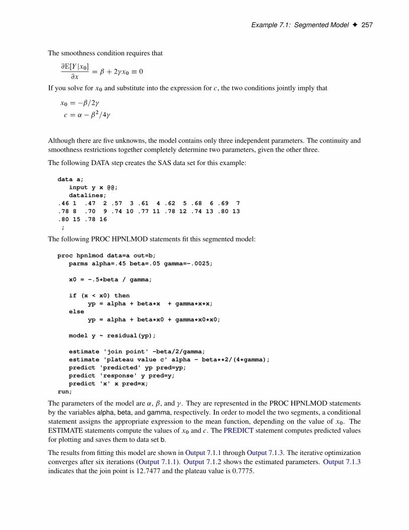
Example 7.1: Segmented Model F 257
The smoothness condition requires that
@EŒY jx0�@x
D ˇ C 2 x0 � 0
If you solve for x0 and substitute into the expression for c, the two conditions jointly imply that
x0 D �ˇ=2
c D ˛ � ˇ2=4
Although there are five unknowns, the model contains only three independent parameters. The continuity andsmoothness restrictions together completely determine two parameters, given the other three.
The following DATA step creates the SAS data set for this example:
data a;input y x @@;datalines;
.46 1 .47 2 .57 3 .61 4 .62 5 .68 6 .69 7
.78 8 .70 9 .74 10 .77 11 .78 12 .74 13 .80 13
.80 15 .78 16;
The following PROC HPNLMOD statements fit this segmented model:
proc hpnlmod data=a out=b;parms alpha=.45 beta=.05 gamma=-.0025;
x0 = -.5*beta / gamma;
if (x < x0) thenyp = alpha + beta*x + gamma*x*x;
elseyp = alpha + beta*x0 + gamma*x0*x0;
model y ~ residual(yp);
estimate 'join point' -beta/2/gamma;estimate 'plateau value c' alpha - beta**2/(4*gamma);predict 'predicted' yp pred=yp;predict 'response' y pred=y;predict 'x' x pred=x;
run;
The parameters of the model are ˛, ˇ, and . They are represented in the PROC HPNLMOD statementsby the variables alpha, beta, and gamma, respectively. In order to model the two segments, a conditionalstatement assigns the appropriate expression to the mean function, depending on the value of x0. TheESTIMATE statements compute the values of x0 and c. The PREDICT statement computes predicted valuesfor plotting and saves them to data set b.
The results from fitting this model are shown in Output 7.1.1 through Output 7.1.3. The iterative optimizationconverges after six iterations (Output 7.1.1). Output 7.1.2 shows the estimated parameters. Output 7.1.3indicates that the join point is 12:7477 and the plateau value is 0:7775.
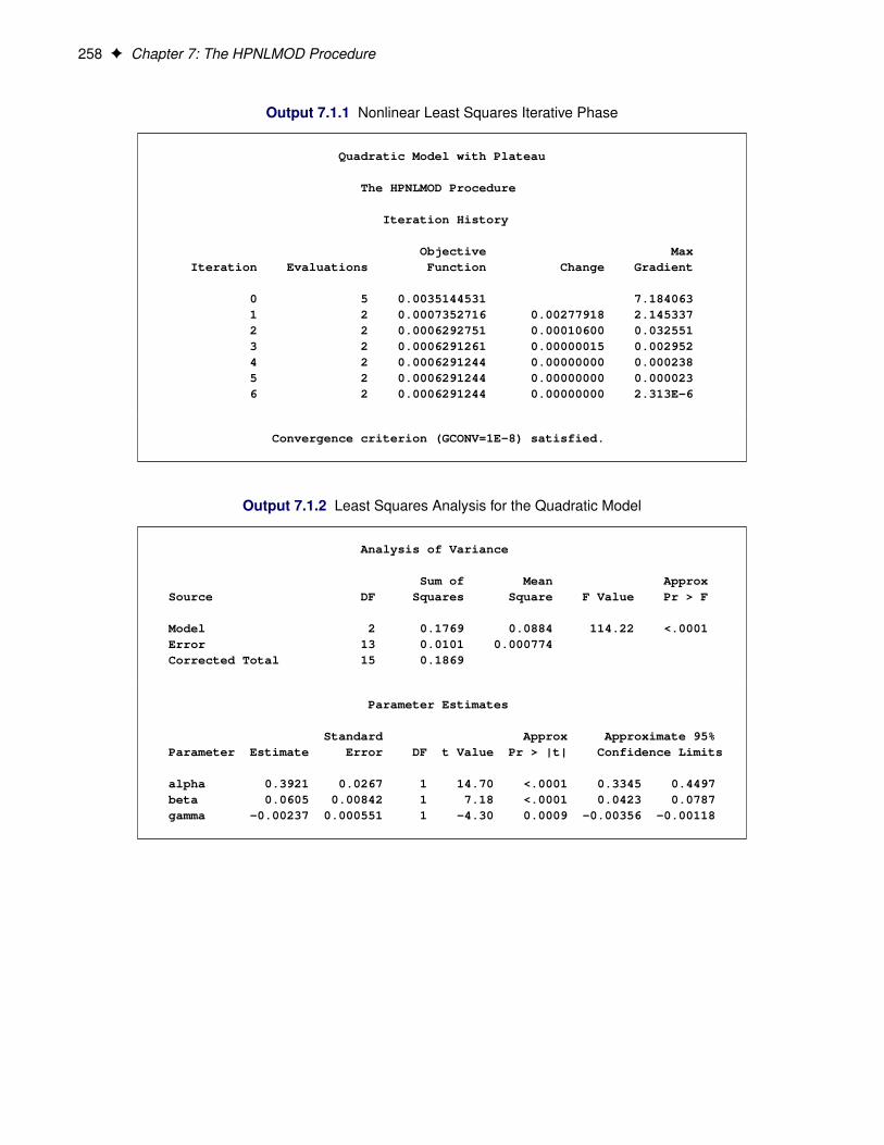
258 F Chapter 7: The HPNLMOD Procedure
Output 7.1.1 Nonlinear Least Squares Iterative Phase
Quadratic Model with Plateau
The HPNLMOD Procedure
Iteration History
Objective MaxIteration Evaluations Function Change Gradient
0 5 0.0035144531 7.1840631 2 0.0007352716 0.00277918 2.1453372 2 0.0006292751 0.00010600 0.0325513 2 0.0006291261 0.00000015 0.0029524 2 0.0006291244 0.00000000 0.0002385 2 0.0006291244 0.00000000 0.0000236 2 0.0006291244 0.00000000 2.313E-6
Convergence criterion (GCONV=1E-8) satisfied.
Output 7.1.2 Least Squares Analysis for the Quadratic Model
Analysis of Variance
Sum of Mean ApproxSource DF Squares Square F Value Pr > F
Model 2 0.1769 0.0884 114.22 <.0001Error 13 0.0101 0.000774Corrected Total 15 0.1869
Parameter Estimates
Standard Approx Approximate 95%Parameter Estimate Error DF t Value Pr > |t| Confidence Limits
alpha 0.3921 0.0267 1 14.70 <.0001 0.3345 0.4497beta 0.0605 0.00842 1 7.18 <.0001 0.0423 0.0787gamma -0.00237 0.000551 1 -4.30 0.0009 -0.00356 -0.00118
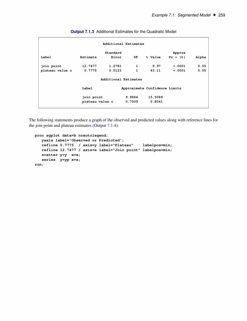
Example 7.1: Segmented Model F 259
Output 7.1.3 Additional Estimates for the Quadratic Model
Additional Estimates
Standard ApproxLabel Estimate Error DF t Value Pr > |t| Alpha
join point 12.7477 1.2781 1 9.97 <.0001 0.05plateau value c 0.7775 0.0123 1 63.11 <.0001 0.05
Additional Estimates
Label Approximate Confidence Limits
join point 9.9864 15.5089plateau value c 0.7509 0.8041
The following statements produce a graph of the observed and predicted values along with reference lines forthe join point and plateau estimates (Output 7.1.4):
proc sgplot data=b noautolegend;yaxis label='Observed or Predicted';refline 0.7775 / axis=y label="Plateau" labelpos=min;refline 12.7477 / axis=x label="Join point" labelpos=min;scatter y=y x=x;series y=yp x=x;
run;
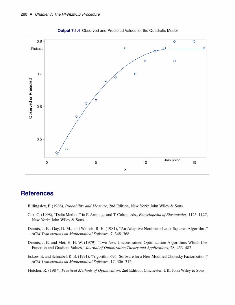
260 F Chapter 7: The HPNLMOD Procedure
Output 7.1.4 Observed and Predicted Values for the Quadratic Model
References
Billingsley, P. (1986), Probability and Measure, 2nd Edition, New York: John Wiley & Sons.
Cox, C. (1998), “Delta Method,” in P. Armitage and T. Colton, eds., Encyclopedia of Biostatistics, 1125–1127,New York: John Wiley & Sons.
Dennis, J. E., Gay, D. M., and Welsch, R. E. (1981), “An Adaptive Nonlinear Least-Squares Algorithm,”ACM Transactions on Mathematical Software, 7, 348–368.
Dennis, J. E. and Mei, H. H. W. (1979), “Two New Unconstrained Optimization Algorithms Which UseFunction and Gradient Values,” Journal of Optimization Theory and Applications, 28, 453–482.
Eskow, E. and Schnabel, R. B. (1991), “Algorithm 695: Software for a New Modified Cholesky Factorization,”ACM Transactions on Mathematical Software, 17, 306–312.
Fletcher, R. (1987), Practical Methods of Optimization, 2nd Edition, Chichester, UK: John Wiley & Sons.

References F 261
Gay, D. M. (1983), “Subroutines for Unconstrained Minimization,” ACM Transactions on MathematicalSoftware, 9, 503–524.
Moré, J. J. (1978), “The Levenberg-Marquardt Algorithm: Implementation and Theory,” in G. A. Watson,ed., Lecture Notes in Mathematics, volume 30, 105–116, Berlin: Springer-Verlag.
Moré, J. J. and Sorensen, D. C. (1983), “Computing a Trust-Region Step,” SIAM Journal on Scientific andStatistical Computing, 4, 553–572.
Ratkowsky, D. (1990), Handbook of Nonlinear Regression Models, New York: Marcel Dekker.

262

Chapter 8
The HPREG Procedure
ContentsOverview: HPREG Procedure . . . . . . . . . . . . . . . . . . . . . . . . . . . . . . . . . 264
PROC HPREG Features . . . . . . . . . . . . . . . . . . . . . . . . . . . . . . . . . 264PROC HPREG Contrasted with Other SAS Procedures . . . . . . . . . . . . . . . . . 265
Getting Started: HPREG Procedure . . . . . . . . . . . . . . . . . . . . . . . . . . . . . . 266Syntax: HPREG Procedure . . . . . . . . . . . . . . . . . . . . . . . . . . . . . . . . . . . 272
PROC HPREG Statement . . . . . . . . . . . . . . . . . . . . . . . . . . . . . . . . 273BY Statement . . . . . . . . . . . . . . . . . . . . . . . . . . . . . . . . . . . . . . 274CODE Statement . . . . . . . . . . . . . . . . . . . . . . . . . . . . . . . . . . . . . 275CLASS Statement . . . . . . . . . . . . . . . . . . . . . . . . . . . . . . . . . . . . 275FREQ Statement . . . . . . . . . . . . . . . . . . . . . . . . . . . . . . . . . . . . . 276ID Statement . . . . . . . . . . . . . . . . . . . . . . . . . . . . . . . . . . . . . . . 276MODEL Statement . . . . . . . . . . . . . . . . . . . . . . . . . . . . . . . . . . . . 276PARTITION Statement . . . . . . . . . . . . . . . . . . . . . . . . . . . . . . . . . 278PERFORMANCE Statement . . . . . . . . . . . . . . . . . . . . . . . . . . . . . . 278SELECTION Statement . . . . . . . . . . . . . . . . . . . . . . . . . . . . . . . . . 278OUTPUT Statement . . . . . . . . . . . . . . . . . . . . . . . . . . . . . . . . . . . 279WEIGHT Statement . . . . . . . . . . . . . . . . . . . . . . . . . . . . . . . . . . . 281
Details: HPREG Procedure . . . . . . . . . . . . . . . . . . . . . . . . . . . . . . . . . . . 282Criteria Used in Model Selection . . . . . . . . . . . . . . . . . . . . . . . . . . . . 282Diagnostic Statistics . . . . . . . . . . . . . . . . . . . . . . . . . . . . . . . . . . . 283Classification Variables and the SPLIT Option . . . . . . . . . . . . . . . . . . . . . 284Using Validation and Test Data . . . . . . . . . . . . . . . . . . . . . . . . . . . . . 286Computational Method . . . . . . . . . . . . . . . . . . . . . . . . . . . . . . . . . . 287Output Data Set . . . . . . . . . . . . . . . . . . . . . . . . . . . . . . . . . . . . . 288Displayed Output . . . . . . . . . . . . . . . . . . . . . . . . . . . . . . . . . . . . . 289ODS Table Names . . . . . . . . . . . . . . . . . . . . . . . . . . . . . . . . . . . . 293
Examples: HPREG Procedure . . . . . . . . . . . . . . . . . . . . . . . . . . . . . . . . . 294Example 8.1: Model Selection with Validation . . . . . . . . . . . . . . . . . . . . . 294Example 8.2: Backward Selection in Single-Machine and Distributed Modes . . . . . 300Example 8.3: Forward-Swap Selection . . . . . . . . . . . . . . . . . . . . . . . . . 304
References . . . . . . . . . . . . . . . . . . . . . . . . . . . . . . . . . . . . . . . . . . . 307

264 F Chapter 8: The HPREG Procedure
Overview: HPREG ProcedureThe HPREG procedure is a high-performance procedure that fits and performs model selection for ordinarylinear least squares models. The models supported are standard independently and identically distributedgeneral linear models, which can contain main effects that consist of both continuous and classificationvariables and interaction effects of these variables. The procedure offers extensive capabilities for customizingthe model selection with a wide variety of selection and stopping criteria, from traditional and computationallyefficient significance-level-based criteria to more computationally intensive validation-based criteria. PROCHPREG also provides a variety of regression diagnostics that are conditional on the selected model.
PROC HPREG runs in either single-machine mode or distributed mode.
NOTE: Distributed mode requires SAS High-Performance Statistics.
PROC HPREG FeaturesThe main features of the HPREG procedure are as follows:
• Model specification
– supports GLM and reference parameterization for classification effects
– supports any degree of interaction (crossed effects) and nested effects
– supports hierarchy among effects
– supports partitioning of data into training, validation, and testing roles
– supports a FREQ statement for grouped analysis
– supports a WEIGHT statement for weighted analysis
• Selection control
– provides multiple effect-selection methods
– enables selection from a very large number of effects (tens of thousands)
– offers selection of individual levels of classification effects
– provides effect selection based on a variety of selection criteria
– provides stopping rules based on a variety of model evaluation criteria
– supports stopping and selection rules based on external validation and leave-one-out crossvalidation
• Display and output
– produces output data sets that contain predicted values, residuals, studentized residuals, confi-dence limits, and influence statistics

PROC HPREG Contrasted with Other SAS Procedures F 265
The HPREG procedure supports the following effect selection methods. For a more detailed description ofthese methods, see the section “Methods” on page 61 in Chapter 3, “Shared Statistical Concepts.”
FORWARD The forward selection method starts with no effects in the model and adds effects.
BACKWARD The backward elimination method starts with all effects in the model and deletes effects.
STEPWISE The stepwise regression method is similar to the FORWARD method except that effectsalready in the model do not necessarily stay there.
FORWARDSWAP The forward swap selection method is a modification of forward selection where beforeany addition step, all pairwise swaps of effects in and out of the current model that improvethe selection criterion are made. When the selection criterion is R square, this methodcoincides with the MAXR method in the REG procedure in SAS/STAT software.
LAR The least angle regression method, like forward selection, starts with no effects in themodel and adds effects. The parameter estimates at any step are “shrunk” when comparedto the corresponding least squares estimates.
LASSO The lasso method adds and deletes parameters based on a version of ordinary least squaresin which the sum of the absolute regression coefficients is constrained. PROC HPREGalso supports adaptive lasso selection where weights are applied to each of the parametersin forming the lasso constraint.
Hybrid versions of LAR and LASSO methods are also supported. They use LAR or LASSO to select themodel, but then estimate the regression coefficients by ordinary weighted least squares.
Because the HPREG procedure is a high-performance analytical procedure, it also does the following:
• enables you to run in distributed mode on a cluster of machines that distribute the data and thecomputations
• enables you to run in single-machine mode on the server where SAS is installed
• exploits all the available cores and concurrent threads, regardless of execution mode
For more information, see the section “Processing Modes” on page 6 in Chapter 2, “Shared Concepts andTopics.”
PROC HPREG Contrasted with Other SAS ProceduresFor general contrasts between SAS High-Performance Analytics procedures and other SAS procedures, seethe section “Common Features of SAS High-Performance Statistical Procedures” on page 40 in Chapter 3,“Shared Statistical Concepts.” The following remarks contrast the HPREG procedure with the GLMSELECT,GLM, and REG procedures in SAS/STAT software.
A major functional difference between the HPREG and REG procedures is that the HPREG procedureenables you to specify general linear models that include classification variables. In this respect it is similarto the GLM and GLMSELECT procedures. In terms of the supported model selection methods, the HPREGprocedure most resembles the GLMSELECT procedure. Like the GLMSELECT procedure but differentfrom the REG procedure, the HPREG procedure supports the LAR and LASSO methods, the ability to use

266 F Chapter 8: The HPREG Procedure
external validation data and cross validation as selection criteria, and extensive options to customize theselection process. The HPREG procedure does not support the MAXR and MINR methods that are availablein the REG procedure. Nor does the HPREG procedure include any support for the all-subset-based methodsthat you can find in the REG procedure.
The CLASS statement in the HPREG procedure permits two parameterizations: the GLM-type parameteriza-tion and a reference parameterization. In contrast to the GLMSELECT, GENMOD, LOGISTIC, and otherprocedures that permit multiple parameterizations, the HPREG procedure does not mix parameterizationsacross the variables in the CLASS statement. In other words, all classification variables are in the sameparameterization, and this parameterization is either the GLM or reference parameterization.
Like the REG procedure but different from the GLMSELECT procedure, the HPREG procedure does notperform model selection by default. If you request model selection by using the SELECTION statementthen the default selection method is stepwise selection based on the SBC criterion. This default matches thedefault method used in PROC GLMSELECT.
As with the REG procedure but not supported with the GLMSELECT procedure, you can request observation-wise residual and influence diagnostics in the OUTPUT statement and variance inflation and tolerancestatistics for the parameter estimates. If the fitted model has been obtained by performing model selection,then these statistics are conditional on the selected model and do not take the variability introduced by theselection process into account.
Getting Started: HPREG ProcedureThe following example is closely modeled on the example in the section “Getting Started: GLMSELECTProcedure” in the SAS/STAT User’s Guide. The data set contains salary and performance information forMajor League Baseball players (excluding pitchers) who played at least one game in both the 1986 and1987 seasons. The salaries are for the 1987 season (Sports Illustrated, April 20, 1987) and the performancemeasures are from 1986 (Collier Books, The 1987 Baseball Encyclopedia Update).
data baseball;length name $ 18;length team $ 12;input name $ 1-18 nAtBat nHits nHome nRuns nRBI nBB
yrMajor crAtBat crHits crHome crRuns crRbi crBBleague $ division $ team $ position $ nOuts nAsstsnError salary;
label name="Player's Name"nAtBat="Times at Bat in 1986"nHits="Hits in 1986"nHome="Home Runs in 1986"nRuns="Runs in 1986"nRBI="RBIs in 1986"nBB="Walks in 1986"yrMajor="Years in the Major Leagues"crAtBat="Career times at bat"crHits="Career Hits"crHome="Career Home Runs"crRuns="Career Runs"crRbi="Career RBIs"
Getting Started: HPREG Procedure F 267
crBB="Career Walks"league="League at the end of 1986"division="Division at the end of 1986"team="Team at the end of 1986"position="Position(s) in 1986"nOuts="Put Outs in 1986"nAssts="Assists in 1986"nError="Errors in 1986"salary="1987 Salary in $ Thousands";logSalary = log(Salary);
datalines;Allanson, Andy 293 66 1 30 29 14
1 293 66 1 30 29 14American East Cleveland C 446 33 20 .
Ashby, Alan 315 81 7 24 38 3914 3449 835 69 321 414 375
National West Houston C 632 43 10 475Davis, Alan 479 130 18 66 72 76
... more lines ...
Wilson, Willie 631 170 9 77 44 3111 4908 1457 30 775 357 249
American West KansasCity CF 408 4 3 1000;
Suppose you want to investigate whether you can model the players’ salaries for the 1987 season based onperformance measures for the previous season. The aim is to obtain a parsimonious model that does notoverfit this particular data, making it useful for prediction. This example shows how you can use PROCHPREG as a starting point for such an analysis. Since the variation of salaries is much greater for the highersalaries, it is appropriate to apply a log transformation to the salaries before doing the model selection.
The following statements select a model with the default settings for stepwise selection:
proc hpreg data=baseball;class league division;model logSalary = nAtBat nHits nHome nRuns nRBI nBB
yrMajor crAtBat crHits crHome crRuns crRbicrBB league division nOuts nAssts nError;
selection method=stepwise;run;
The default output from this analysis is presented in Figure 8.1 through Figure 8.5.
Figure 8.1 Performance, Model, and Selection Information
The HPREG Procedure
Performance Information
Execution Mode Single-MachineNumber of Threads 4
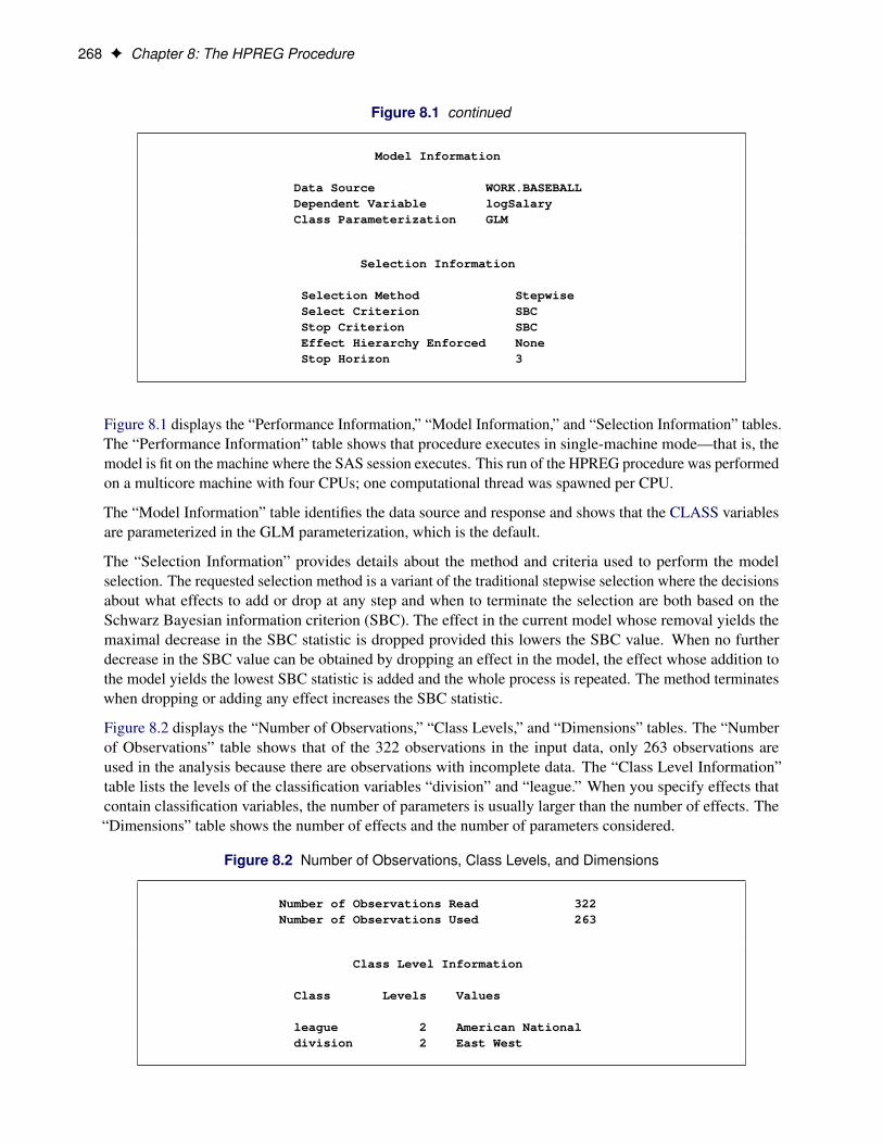
268 F Chapter 8: The HPREG Procedure
Figure 8.1 continued
Model Information
Data Source WORK.BASEBALLDependent Variable logSalaryClass Parameterization GLM
Selection Information
Selection Method StepwiseSelect Criterion SBCStop Criterion SBCEffect Hierarchy Enforced NoneStop Horizon 3
Figure 8.1 displays the “Performance Information,” “Model Information,” and “Selection Information” tables.The “Performance Information” table shows that procedure executes in single-machine mode—that is, themodel is fit on the machine where the SAS session executes. This run of the HPREG procedure was performedon a multicore machine with four CPUs; one computational thread was spawned per CPU.
The “Model Information” table identifies the data source and response and shows that the CLASS variablesare parameterized in the GLM parameterization, which is the default.
The “Selection Information” provides details about the method and criteria used to perform the modelselection. The requested selection method is a variant of the traditional stepwise selection where the decisionsabout what effects to add or drop at any step and when to terminate the selection are both based on theSchwarz Bayesian information criterion (SBC). The effect in the current model whose removal yields themaximal decrease in the SBC statistic is dropped provided this lowers the SBC value. When no furtherdecrease in the SBC value can be obtained by dropping an effect in the model, the effect whose addition tothe model yields the lowest SBC statistic is added and the whole process is repeated. The method terminateswhen dropping or adding any effect increases the SBC statistic.
Figure 8.2 displays the “Number of Observations,” “Class Levels,” and “Dimensions” tables. The “Numberof Observations” table shows that of the 322 observations in the input data, only 263 observations areused in the analysis because there are observations with incomplete data. The “Class Level Information”table lists the levels of the classification variables “division” and “league.” When you specify effects thatcontain classification variables, the number of parameters is usually larger than the number of effects. The“Dimensions” table shows the number of effects and the number of parameters considered.
Figure 8.2 Number of Observations, Class Levels, and Dimensions
Number of Observations Read 322Number of Observations Used 263
Class Level Information
Class Levels Values
league 2 American Nationaldivision 2 East West
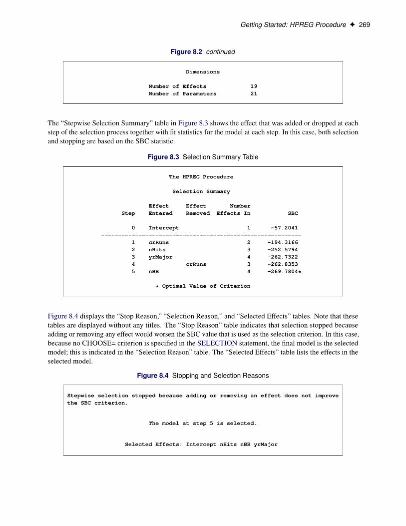
Getting Started: HPREG Procedure F 269
Figure 8.2 continued
Dimensions
Number of Effects 19Number of Parameters 21
The “Stepwise Selection Summary” table in Figure 8.3 shows the effect that was added or dropped at eachstep of the selection process together with fit statistics for the model at each step. In this case, both selectionand stopping are based on the SBC statistic.
Figure 8.3 Selection Summary Table
The HPREG Procedure
Selection Summary
Effect Effect NumberStep Entered Removed Effects In SBC
0 Intercept 1 -57.2041-----------------------------------------------------------
1 crRuns 2 -194.31662 nHits 3 -252.57943 yrMajor 4 -262.73224 crRuns 3 -262.83535 nBB 4 -269.7804*
* Optimal Value of Criterion
Figure 8.4 displays the “Stop Reason,” “Selection Reason,” and “Selected Effects” tables. Note that thesetables are displayed without any titles. The “Stop Reason” table indicates that selection stopped becauseadding or removing any effect would worsen the SBC value that is used as the selection criterion. In this case,because no CHOOSE= criterion is specified in the SELECTION statement, the final model is the selectedmodel; this is indicated in the “Selection Reason” table. The “Selected Effects” table lists the effects in theselected model.
Figure 8.4 Stopping and Selection Reasons
Stepwise selection stopped because adding or removing an effect does not improvethe SBC criterion.
The model at step 5 is selected.
Selected Effects: Intercept nHits nBB yrMajor

270 F Chapter 8: The HPREG Procedure
The “Analysis of Variance,” “Fit Statistics,” and “Parameter Estimates” tables shown in Figure 8.5 give detailsof the selected model.
Figure 8.5 Details of the Selected Model
Analysis of Variance
Sum of MeanSource DF Squares Square F Value Pr > F
Model 3 120.52553 40.17518 120.12 <.0001Error 259 86.62820 0.33447Corrected Total 262 207.15373
Root MSE 0.57834R-Square 0.58182Adj R-Sq 0.57697AIC -19.06903AICC -18.83557SBC -269.78041ASE 0.32938
Parameter Estimates
StandardParameter DF Estimate Error t Value Pr > |t|
Intercept 1 4.013911 0.111290 36.07 <.0001nHits 1 0.007929 0.000994 7.98 <.0001nBB 1 0.007280 0.002049 3.55 0.0005yrMajor 1 0.100663 0.007551 13.33 <.0001
You might want to examine regression diagnostics for the selected model to investigate whether collinearityamong the selected parameters or the presence of outlying or high leverage observations might be impactingthe fit produced. The following statements include some options and statements to obtain these diagnostics:
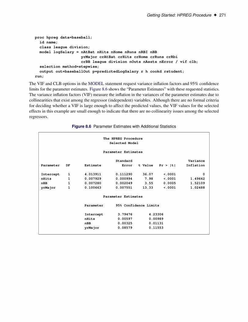
Getting Started: HPREG Procedure F 271
proc hpreg data=baseball;id name;class league division;model logSalary = nAtBat nHits nHome nRuns nRBI nBB
yrMajor crAtBat crHits crHome crRuns crRbicrBB league division nOuts nAssts nError / vif clb;
selection method=stepwise;output out=baseballOut p=predictedLogSalary r h cookd rstudent;
run;
The VIF and CLB options in the MODEL statement request variance inflation factors and 95% confidencelimits for the parameter estimates. Figure 8.6 shows the “Parameter Estimates” with these requested statistics.The variance inflation factors (VIF) measure the inflation in the variances of the parameter estimates due tocollinearities that exist among the regressor (independent) variables. Although there are no formal criteriafor deciding whether a VIF is large enough to affect the predicted values, the VIF values for the selectedeffects in this example are small enough to indicate that there are no collinearity issues among the selectedregressors.
Figure 8.6 Parameter Estimates with Additional Statistics
The HPREG ProcedureSelected Model
Parameter Estimates
Standard VarianceParameter DF Estimate Error t Value Pr > |t| Inflation
Intercept 1 4.013911 0.111290 36.07 <.0001 0nHits 1 0.007929 0.000994 7.98 <.0001 1.49642nBB 1 0.007280 0.002049 3.55 0.0005 1.52109yrMajor 1 0.100663 0.007551 13.33 <.0001 1.02488
Parameter Estimates
Parameter 95% Confidence Limits
Intercept 3.79476 4.23306nHits 0.00597 0.00989nBB 0.00325 0.01131yrMajor 0.08579 0.11553

272 F Chapter 8: The HPREG Procedure
By default, High-Performance Analytics procedures do not include all variables from the input data set inoutput data sets. The ID statement specifies that the variable name in the input data set be added as anidentification variable in the baseballOut data set that is produced by the OUTPUT statement. In addition tothis variable, the OUTPUT statement requests that predicted values, raw residuals, leverage values, Cook’s Dstatistics, and studentized residuals be added in the output data set. Note that default names are used for thesestatistics except for the predicted values for which a specified name, predictedLogSalary, is supplied. Thefollowing statements use PROC PRINT to display the first five observations of this output data set:
proc print data=baseballOut(obs=5);run;
Figure 8.7 First 5 Observations of the baseballOut Data Set
predictedObs name LogSalary Residual H COOKD RSTUDENT
1 Allanson, Andy 4.73980 . 0.016087 . .2 Ashby, Alan 6.34935 -0.18603 0.012645 .000335535 -0.323163 Davis, Alan 5.89993 0.27385 0.019909 .001161794 0.477594 Dawson, Andre 6.50852 -0.29392 0.011060 .000730178 -0.510315 Galarraga, Andres 5.12344 -0.60711 0.009684 .002720358 -1.05510
Syntax: HPREG ProcedureThe following statements are available in the HPREG procedure:
PROC HPREG < options > ;BY variables ;CODE < options > ;CLASS variables ;MODEL dependent = < effects > < / model-options > ;OUTPUT < OUT=SAS-data-set >
< keyword < =name > >. . .< keyword < =name > > < / options > ;
PARTITION < partition-options > ;PERFORMANCE performance-options ;SELECTION selection-options ;FREQ variable ;ID variables ;WEIGHT variable ;
The PROC HPREG statement and a single MODEL statement are required. All other statements are optional.The CLASS statement can appear multiple times. If a CLASS statement is specified, it must precede theMODEL statement.
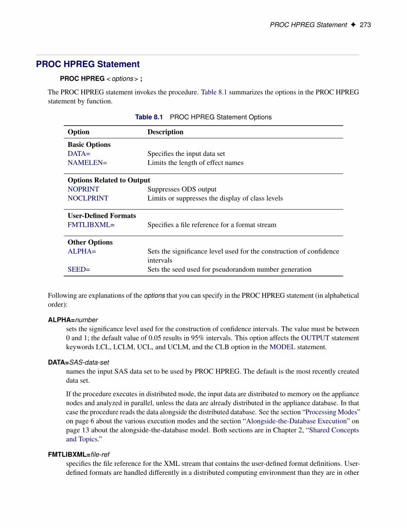
PROC HPREG Statement F 273
PROC HPREG StatementPROC HPREG < options > ;
The PROC HPREG statement invokes the procedure. Table 8.1 summarizes the options in the PROC HPREGstatement by function.
Table 8.1 PROC HPREG Statement Options
Option Description
Basic OptionsDATA= Specifies the input data setNAMELEN= Limits the length of effect names
Options Related to OutputNOPRINT Suppresses ODS outputNOCLPRINT Limits or suppresses the display of class levels
User-Defined FormatsFMTLIBXML= Specifies a file reference for a format stream
Other OptionsALPHA= Sets the significance level used for the construction of confidence
intervalsSEED= Sets the seed used for pseudorandom number generation
Following are explanations of the options that you can specify in the PROC HPREG statement (in alphabeticalorder):
ALPHA=numbersets the significance level used for the construction of confidence intervals. The value must be between0 and 1; the default value of 0.05 results in 95% intervals. This option affects the OUTPUT statementkeywords LCL, LCLM, UCL, and UCLM, and the CLB option in the MODEL statement.
DATA=SAS-data-setnames the input SAS data set to be used by PROC HPREG. The default is the most recently createddata set.
If the procedure executes in distributed mode, the input data are distributed to memory on the appliancenodes and analyzed in parallel, unless the data are already distributed in the appliance database. In thatcase the procedure reads the data alongside the distributed database. See the section “Processing Modes”on page 6 about the various execution modes and the section “Alongside-the-Database Execution” onpage 13 about the alongside-the-database model. Both sections are in Chapter 2, “Shared Conceptsand Topics.”
FMTLIBXML=file-refspecifies the file reference for the XML stream that contains the user-defined format definitions. User-defined formats are handled differently in a distributed computing environment than they are in other
274 F Chapter 8: The HPREG Procedure
SAS products. See the section “Working with Formats” on page 32 in Chapter 2, “Shared Conceptsand Topics,” for details about how to generate a XML stream for your formats.
NAMELEN=numberspecifies the length to which long effect names are shortened. The default and minimum value is 20.
NOCLPRINT< =number >suppresses the display of the “Class Level Information” table if you do not specify number. If youspecify number, the values of the classification variables are displayed for only those variables whosenumber of levels is less than number. Specifying a number helps to reduce the size of the “Class LevelInformation” table if some classification variables have a large number of levels.
NOPRINTsuppresses the generation of ODS output.
SEED=numberspecifies an integer used to start the pseudorandom number generator for random partitioning of datafor training, testing, and validation. If you do not specify a seed, or if you specify a value less than orequal to 0, the seed is generated from reading the time of day from the computer’s clock.
BY StatementBY variables ;
You can specify a BY statement in PROC HPREG to obtain separate analyses of observations in groups thatare defined by the BY variables. When a BY statement appears, PROC HPREG expects the input data set tobe sorted in order of the BY variables. If you specify more than one BY statement, only the last one specifiedis used.
If your input data set is not sorted in ascending order, use one of the following alternatives:
• Sort the data by using the SORT procedure and a similar BY statement.
• Specify the NOTSORTED or DESCENDING option in the BY statement for the HPREG procedure.The NOTSORTED option does not mean that the data are unsorted but rather that the data are arrangedin groups (according to values of the BY variables) and that these groups are not necessarily inalphabetical or increasing numeric order.
• Create an index on the BY variables by using the DATASETS procedure (in Base SAS software).
BY statement processing is not supported when the HPREG procedure runs alongside the database oralongside the Hadoop Distributed File System (HDFS). These modes are used if the input data are stored in adatabase or HDFS and the grid host is the appliance that houses the data.
For more information about BY-group processing, see SAS Language Reference: Concepts. For moreinformation about the DATASETS procedure, see Base SAS Procedures Guide.
CLASS Statement F 275
CODE StatementCODE < options > ;
The CODE statement enables you to write SAS DATA step code for computing predicted values of the fittedmodel either to a file or to a catalog entry. This code can then be included in a DATA step to score new data.
Table 8.2 summarizes the options available in the CODE statement.
Table 8.2 CODE Statement Options
Option Description
CATALOG= Names the catalog entry where the generated code is savedDUMMIES Retains the dummy variables in the data setERROR Computes the error functionFILE= Names the file where the generated code is savedFORMAT= Specifies the numeric format for the regression coefficientsGROUP= Specifies the group identifier for array names and statement labelsIMPUTE Imputes predicted values for observations with missing or invalid
covariatesLINESIZE= Specifies the line size of the generated codeLOOKUP= Specifies the algorithm for looking up CLASS levelsRESIDUAL Computes residuals
For more information about the syntax of the CODE statement, see the section “CODE Statement” (Chap-ter 19, SAS/STAT User’s Guide).
CLASS StatementCLASS variable < (options) >: : : < variable < (options) > > < / global-options > ;
The CLASS statement names the classification variables to be used as explanatory variables in the analysis.The CLASS statement must precede the MODEL statement.
The CLASS statement for SAS High-Performance Analytics procedures is documented in the section “CLASSStatement” on page 40 of Chapter 3, “Shared Statistical Concepts.” The HPREG procedure also supports thefollowing global-option in the CLASS statement:
UPCASEuppercases the values of character-valued CLASS variables before levelizing them. For example, if theUPCASE option is in effect and a CLASS variable can take the values ‘a’, ‘A’, and ‘b’, then ‘a’ and ‘A’represent the same level and the CLASS variable is treated as having only two values: ‘A’ and ‘B’.

276 F Chapter 8: The HPREG Procedure
FREQ StatementFREQ variable ;
The variable in the FREQ statement identifies a numeric variable in the data set that contains the frequencyof occurrence for each observation. SAS High-Performance Analytics procedures that support the FREQstatement treat each observation as if it appeared f times, where f is the value of the FREQ variable for theobservation. If the frequency value is not an integer, it is truncated to an integer. If the frequency value is lessthan 1 or missing, the observation is not used in the analysis. When the FREQ statement is not specified,each observation is assigned a frequency of 1.
ID StatementID variables ;
The ID statement lists one or more variables from the input data set that are transferred to output data setscreated by SAS High-Performance Analytics procedures, provided that the output data set produces one (ormore) records per input observation.
For documentation on the common ID statement in SAS High-Performance Analytics procedures, see thesection “ID Statement” on page 44 in Chapter 3, “Shared Statistical Concepts.”
MODEL StatementMODEL dependent=< effects > / < options > ;
The MODEL statement names the dependent variable and the explanatory effects, including covariates,main effects, interactions, and nested effects. If you omit the explanatory effects, the procedure fits anintercept-only model.
After the keyword MODEL, the dependent (response) variable is specified, followed by an equal sign. Theexplanatory effects follow the equal sign. For information about constructing the model effects, see thesection “Specification and Parameterization of Model Effects” on page 52, of Chapter 3, “Shared StatisticalConcepts.”
You can specify the following options in the MODEL statement after a slash (/):
CLBrequests the 100.1�˛/% upper and lower confidence limits for the parameter estimates. By default, the95% limits are computed; the ALPHA= option in the PROC HPREG statement can be used to changethe ˛ level. The CLB option is not supported when you request METHOD=LAR or METHOD=LASSOin the SELECTION statement.

MODEL Statement F 277
INCLUDE=n
INCLUDE=single-effect
INCLUDE=(effects)forces effects to be included in all models. If you specify INCLUDE=n, then the first n effects listedin the MODEL statement are included in all models. If you specify INCLUDE=single-effect or ifyou specify a list of effects within parentheses, then the specified effects are forced into all models.The effects that you specify in the INCLUDE= option must be explanatory effects defined in theMODELstatement before the slash (/). The INCLUDE= option is not available when you specifyMETHOD=LAR or METHOD=LASSO in the SELECTION statement.
NOINTsuppresses the intercept term that is otherwise included in the model.
ORDERSELECTspecifies that, for the selected model, effects be displayed in the order in which they first enteredthe model. If you do not specify the ORDERSELECT option, then effects in the selected model aredisplayed in the order in which they appear in the MODEL statement.
START=n
START=single-effect
START=(effects)is used to begin the selection process in the FORWARD, FORWARDSWAP, and STEPWISE selectionmethods from the initial model that you designate. If you specify START=n, then the starting modelconsists of the first n effects listed in the MODEL statement. If you specify START=single-effect orif you specify a list of effects within parentheses, then the starting model consists of these specifiedeffects. The effects that you specify in the START= option must be explanatory effects defined inthe MODELstatement before the slash (/). The START= option is not available when you specifyMETHOD=BACKWARD, METHOD=LAR, or METHOD=LASSO in the SELECTION statement.
STBproduces standardized regression coefficients. A standardized regression coefficient is computed bydividing a parameter estimate by the ratio of the sample standard deviation of the dependent variableto the sample standard deviation of the regressor.
TOLproduces tolerance values for the estimates. Tolerance for a parameter is defined as 1 � R2, whereR2 is obtained from the regression of the parameter on all other parameters in the model. The TOLoption is not supported when you request METHOD=LAR or METHOD=LASSO in the SELECTIONstatement.
VIFproduces variance inflation factors with the parameter estimates. Variance inflation is the reciprocal oftolerance. The VIF option is not supported when you request METHOD=LAR or METHOD=LASSOin the SELECTION statement.
278 F Chapter 8: The HPREG Procedure
PARTITION StatementPARTITION < partition-options > ;
The PARTITION statement specifies how observations in the input data set are logically partitioned intodisjoint subsets for model training, validation, and testing. Either you can designate a variable in the inputdata set and a set of formatted values of that variable to determine the role of each observation, or you canspecify proportions to use for random assignment of observations for each role.
The following mutually exclusive partition-options are available:
ROLEVAR | ROLE=variable(< TEST=’value’ > < TRAIN=’value’ > < VALIDATE=’value’ >)names the variable in the input data set whose values are used to assign roles to each observation.The formatted values of this variable that are used to assign observations roles are specified in theTEST=, TRAIN=, and VALIDATE= suboptions. If you do not specify the TRAIN= suboption, then allobservations whose role is not determined by the TEST= or VALIDATE= suboptions are assigned totraining.
FRACTION(< TEST=fraction > < VALIDATE=fraction >)requests that specified proportions of the observations in the input data set be randomly assignedtraining and validation roles. You specify the proportions for testing and validation by using the TEST=and VALIDATE= suboptions. If you specify both the TEST= and the VALIDATE= suboptions, thenthe sum of the specified fractions must be less than 1 and the remaining fraction of the observations areassigned to the training role.
PERFORMANCE StatementPERFORMANCE < performance-options > ;
The PERFORMANCE statement defines performance parameters for multithreaded and distributed comput-ing, passes variables that describe the distributed computing environment, and requests detailed results aboutthe performance characteristics of the HPREG procedure.
You can also use the PERFORMANCE statement to control whether the HPREG procedure executes insingle-machine mode or distributed mode.
The PERFORMANCE statement is documented further in the section “PERFORMANCE Statement” onpage 34.
SELECTION StatementSELECTION < options > ;
The SELECTION statement performs variable selection. The statement is fully documented in the section“SELECTION Statement” on page 45 in Chapter 3, “Shared Statistical Concepts.”
OUTPUT Statement F 279
The HPREG procedure supports the following variable selection methods in the METHOD= option in theSELECTION statement:
NONE No model selection.
FORWARD The forward selection method starts with no effects in the model and adds effects.
BACKWARD The backward elimination method starts with all effects in the model and deletes effects.
STEPWISE The stepwise regression method is similar to the FORWARD method except that effectsalready in the model do not necessarily stay there.
FORWARDSWAP The forward-swap selection method is an extension of the forward selection method.Before any addition step, PROC HPREG makes all pairwise swaps of effects in and out ofthe current model that improve the selection criterion. When the selection criterion is Rsquare, this method is the same as the MAXR method in the REG procedure in SAS/STATsoftware.
LAR The least angle regression method, like forward selection, starts with no effects in themodel and adds effects. The parameter estimates at any step are “shrunk” when comparedto the corresponding least squares estimates. If the model contains classification variables,then these classification variables are split. See the SPLIT option in the CLASS statementfor details.
LASSO The lasso method adds and deletes parameters based on a version of ordinary least squareswhere the sum of the absolute regression coefficients is constrained. If the model containsclassification variables, then these classification variables are split. See the SPLIT optionin the CLASS statement for details.
The DETAILS=ALL and DETAILS=STEPS options produce the “ANOVA,” “Fit Statistics,” and “ParameterEstimates” tables, which provide information about the model that is selected at each step of the selectionprocess.
OUTPUT StatementOUTPUT < OUT=SAS-data-set >
< COPYVARS=(variables) >< keyword < =name > >. . . < keyword < =name > > ;
The OUTPUT statement creates a data set that contains observationwise statistics, which are computed afterfitting the model. The variables in the input data set are not included in the output data set to avoid dataduplication for large data sets; however, variables specified in the ID statement or COPYVARS= option areincluded.
If the input data are in distributed form, where access of data in a particular order cannot be guaranteed, theHPREG procedure copies the distribution or partition key to the output data set so that its contents can bejoined with the input data.
The output statistics are computed based on the parameter estimates for the selected model.
280 F Chapter 8: The HPREG Procedure
You can specify the following syntax elements in the OUTPUT statement:
OUT=SAS-data-set
DATA=SAS-data-setspecifies the name of the output data set. If the OUT= (or DATA=) option is omitted, the procedureuses the DATAn convention to name the output data set.
COPYVAR=variable
COPYVARS=(variables)transfers one or more variables from the input data set to the output data set. Variables named in an IDstatement are also copied from the input data set to the output data set.
keyword < =name >specifies the statistics to include in the output data set and optionally names the new variables thatcontain the statistics. Specify a keyword for each desired statistic (see the following list of keywords),followed optionally by an equal sign and a variable to contain the statistic.
If you specify keyword=name, the new variable that contains the requested statistic has the specifiedname. If you omit the optional =name after a keyword, then a default name is used.
The following are valid values for keyword to request statistics that are available with all selectionmethods:
PREDICTED
PRED
Prequests predicted values for the response variable. The default name is pred.
RESIDUAL
RESID
Rrequests the residual, calculated as ACTUAL–PREDICTED. The default name is residual.
ROLErequests a numeric variable that indicates the role played by each observation in fitting the model.The default name is role. For each observation the interpretation of this variable is shown inTable 8.3:
Table 8.3 Role Interpretation
Value Observation Role
0 Not used1 Training2 Validation3 Testing
If you do not partition the input data by using a PARTITION statement, then the role variablevalue is 1 for observations used in fitting the model, and 0 for observations that have at least onemissing or invalid value for the response, regressors, frequency or weight variables.
WEIGHT Statement F 281
In addition to the preceding statistics, you can also use the keywords listed in Table 8.4 in the OUTPUTstatement to obtain additional statistics. These statistics are not available if you use METHOD=LAR orMETHOD=LASSO in the SELECTION statement, unless you also specify the LSCOEFFS option. Seethe section “Diagnostic Statistics” on page 283 for computational formulas. All the statistics available inthe OUTPUT statement are conditional on the selected model and do not take into account the variabilityintroduced by doing model selection.
Table 8.4 Keywords for OUTPUT Statement
Keyword Description
COOKD Cook’s D influence statisticCOVRATIO Standard influence of observation on covariance of betasDFFIT Standard influence of observation on predicted valueH Leverage, xi .X0X/�1x0iLCL Lower bound of a 100.1 � ˛/% confidence interval for an
individual prediction. This includes the variance of theerror, as well as the variance of the parameter estimates.
LCLM Lower bound of a 100.1 � ˛/% confidence interval for theexpected value (mean) of the dependent variable
PRESS ith residual divided by .1 � h/, where h is the leverage,and where the model has been refit without the ithobservation
RSTUDENT A studentized residual with the current observation deletedSTDI Standard error of the individual predicted valueSTDP Standard error of the mean predicted valueSTDR Standard error of the residualSTUDENT Studentized residuals, which are the residuals divided by their
standard errorsUCL Upper bound of a 100.1 � ˛/% confidence interval for an
individual predictionUCLM Upper bound of a 100.1 � ˛/% confidence interval for the
expected value (mean) of the dependent variable
WEIGHT StatementWEIGHT variable ;
The variable in the WEIGHT statement is used as a weight to perform a weighted analysis of the data.Observations with nonpositive or missing weights are not included in the analysis. If a WEIGHT statement isnot included, all observations used in the analysis are assigned a weight of 1.

282 F Chapter 8: The HPREG Procedure
Details: HPREG Procedure
Criteria Used in Model SelectionThe HPREG procedure supports a variety of fit statistics that you can specify as criteria for the CHOOSE=,SELECT=, and STOP= options in the SELECTION statement. The following statistics are available:
ADJRSQ Adjusted R-square statistic (Darlington 1968; Judge et al. 1985)
AIC Akaike’s information criterion (Akaike 1969; Judge et al. 1985)
AICC Corrected Akaike’s information criterion (Hurvich and Tsai 1989)
BIC | SBC Schwarz Bayesian information criterion (Schwarz 1978; Judge et al. 1985)
CP Mallows Cp statistic (Mallows 1973; Hocking 1976)
PRESS Predicted residual sum of squares statistic
RSQUARE R-square statistic (Darlington 1968; Judge et al. 1985)
SL Significance used to assess an effect’s contribution to the fit when it is added to or removedfrom a model
VALIDATE Average square error over the validation data
When you use SL as a criterion for effect selection, the definition depends on whether an effect is beingconsidered as a drop or an add candidate. If the current model has p parameters excluding the intercept,and if you denote its residual sum of squares by RSSp and you add an effect with k degrees of freedom anddenote the residual sum of squares of the resulting model by RSSpCk , then the F statistic for entry with knumerator degrees of freedom and n � .p C k/ � 1 denominator degrees of freedom is given by
F D.RSSp � RSSpCk/=k
RSSpCk=.n � .p C k/ � 1/
where n is number of observations used in the analysis. The significance level for entry is the p-value ofthis F statistic, and is deemed significant if it is smaller than the SLENTRY limit. Among several such addcandidates, the effect with the smallest p-value (most significant) is deemed best.
If you drop an effect with k degrees of freedom and denote the residual sum of squares of the resulting modelby RSSp�k , then the F statistic for removal with k numerator degrees of freedom and n�p� k denominatordegrees of freedom is given by
F D.RSSp�k � RSSp/=k
RSSp=.n � p � k/
where n is number of observations used in the analysis. The significance level for removal is the p-valueof this F statistic, and the effect is deemed not significant if this p-value is larger than the SLSTAY limit.Among several such removal candidates, the effect with the largest p-value (least significant) is deemed thebest removal candidate.
It is known that the “F-to-enter” and “F-to-delete” statistics do not follow an F distribution (Draper, Guttman,and Kanemasu 1971).. Hence the SLENTRY and SLSTAY values cannot reliably be viewed as probabilities.

Diagnostic Statistics F 283
One way to address this difficulty is to replace hypothesis testing as a means of selecting a model withinformation criteria or out-of-sample prediction criteria. While Harrell (2001) points out that informationcriteria were developed for comparing only prespecified models, Burnham and Anderson (2002) note thatAIC criteria have routinely been used for several decades for performing model selection in time seriesanalysis.
Table 8.5 provides formulas and definitions for these fit statistics.
Table 8.5 Formulas and Definitions for Model Fit Summary Statistics
Statistic Definition or Formula
n Number of observationsp Number of parameters including the interceptO�2 Estimate of pure error variance from fitting the full model
SST Total sum of squares corrected for the mean for thedependent variable
SSE Error sum of squares
ASESSEn
MSESSEn � p
R2 1 �SSESST
ADJRSQ 1 �.n � 1/.1 �R2/
n � p
AIC n ln�
SSEn
�C 2p
AICC 1C ln�
SSEn
�C2.p C 1/
n � p � 2
CP .Cp/SSEO�2C 2p � n
PRESSnXiD1
r2i.1 � hi /2
where
ri D residual at observation i andhi D leverage of observation i D xi .X0X/�x0i
RMSEp
MSE
SBC n ln�
SSEn
�C p ln.n/
Diagnostic StatisticsThis section gathers the formulas for the statistics available in the OUTPUT statement. All the statisticsavailable in the OUTPUT statement are conditional on the selected model and do not take into account thevariability introduced by doing model selection.
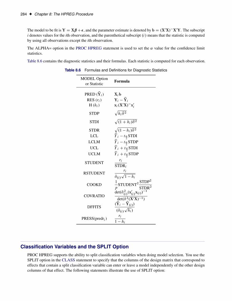
284 F Chapter 8: The HPREG Procedure
The model to be fit is Y D XˇC�, and the parameter estimate is denoted by b D .X0X/�X0Y. The subscripti denotes values for the ith observation, and the parenthetical subscript .i/means that the statistic is computedby using all observations except the ith observation.
The ALPHA= option in the PROC HPREG statement is used to set the ˛ value for the confidence limitstatistics.
Table 8.6 contains the diagnostic statistics and their formulas. Each statistic is computed for each observation.
Table 8.6 Formulas and Definitions for Diagnostic Statistics
MODEL Optionor Statistic
Formula
PRED (bYi ) XibRES (ri ) Yi � bYiH (hi ) xi .X0X/�x0i
STDPphib�2
STDIp.1C hi /b�2
STDRp.1 � hi /b�2
LCL bY i � t˛2
STDILCLM bY i � t˛
2STDP
UCL bY i C t˛2
STDIUCLM bY i C t˛
2STDP
STUDENTri
STDRi
RSTUDENTri
O�.i/p1 � hi
COOKD1
pSTUDENT2
STDP2
STDR2
COVRATIOdet. O�2
.i/.x0.i/
x.i//�1
det. O�2.X0X/�1/
DFFITS.bYi � bY.i//. O�.i/phi /
PRESS(predri )ri
1 � hi
Classification Variables and the SPLIT OptionPROC HPREG supports the ability to split classification variables when doing model selection. You use theSPLIT option in the CLASS statement to specify that the columns of the design matrix that correspond toeffects that contain a split classification variable can enter or leave a model independently of the other designcolumns of that effect. The following statements illustrate the use of SPLIT option:
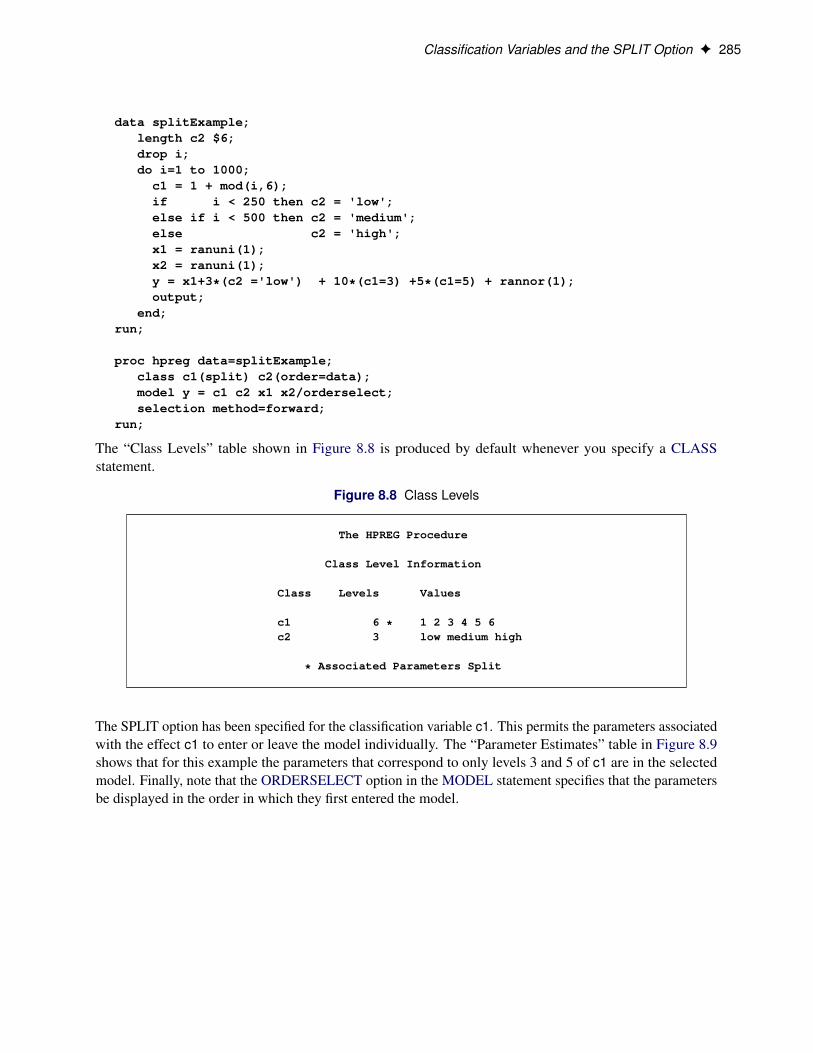
Classification Variables and the SPLIT Option F 285
data splitExample;length c2 $6;drop i;do i=1 to 1000;
c1 = 1 + mod(i,6);if i < 250 then c2 = 'low';else if i < 500 then c2 = 'medium';else c2 = 'high';x1 = ranuni(1);x2 = ranuni(1);y = x1+3*(c2 ='low') + 10*(c1=3) +5*(c1=5) + rannor(1);output;
end;run;
proc hpreg data=splitExample;class c1(split) c2(order=data);model y = c1 c2 x1 x2/orderselect;selection method=forward;
run;
The “Class Levels” table shown in Figure 8.8 is produced by default whenever you specify a CLASSstatement.
Figure 8.8 Class Levels
The HPREG Procedure
Class Level Information
Class Levels Values
c1 6 * 1 2 3 4 5 6c2 3 low medium high
* Associated Parameters Split
The SPLIT option has been specified for the classification variable c1. This permits the parameters associatedwith the effect c1 to enter or leave the model individually. The “Parameter Estimates” table in Figure 8.9shows that for this example the parameters that correspond to only levels 3 and 5 of c1 are in the selectedmodel. Finally, note that the ORDERSELECT option in the MODEL statement specifies that the parametersbe displayed in the order in which they first entered the model.
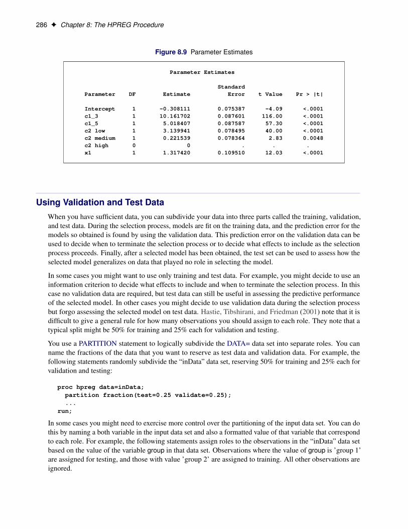
286 F Chapter 8: The HPREG Procedure
Figure 8.9 Parameter Estimates
Parameter Estimates
StandardParameter DF Estimate Error t Value Pr > |t|
Intercept 1 -0.308111 0.075387 -4.09 <.0001c1_3 1 10.161702 0.087601 116.00 <.0001c1_5 1 5.018407 0.087587 57.30 <.0001c2 low 1 3.139941 0.078495 40.00 <.0001c2 medium 1 0.221539 0.078364 2.83 0.0048c2 high 0 0 . . .x1 1 1.317420 0.109510 12.03 <.0001
Using Validation and Test DataWhen you have sufficient data, you can subdivide your data into three parts called the training, validation,and test data. During the selection process, models are fit on the training data, and the prediction error for themodels so obtained is found by using the validation data. This prediction error on the validation data can beused to decide when to terminate the selection process or to decide what effects to include as the selectionprocess proceeds. Finally, after a selected model has been obtained, the test set can be used to assess how theselected model generalizes on data that played no role in selecting the model.
In some cases you might want to use only training and test data. For example, you might decide to use aninformation criterion to decide what effects to include and when to terminate the selection process. In thiscase no validation data are required, but test data can still be useful in assessing the predictive performanceof the selected model. In other cases you might decide to use validation data during the selection processbut forgo assessing the selected model on test data. Hastie, Tibshirani, and Friedman (2001) note that it isdifficult to give a general rule for how many observations you should assign to each role. They note that atypical split might be 50% for training and 25% each for validation and testing.
You use a PARTITION statement to logically subdivide the DATA= data set into separate roles. You canname the fractions of the data that you want to reserve as test data and validation data. For example, thefollowing statements randomly subdivide the “inData” data set, reserving 50% for training and 25% each forvalidation and testing:
proc hpreg data=inData;partition fraction(test=0.25 validate=0.25);...
run;
In some cases you might need to exercise more control over the partitioning of the input data set. You can dothis by naming a both variable in the input data set and also a formatted value of that variable that correspondto each role. For example, the following statements assign roles to the observations in the “inData” data setbased on the value of the variable group in that data set. Observations where the value of group is ’group 1’are assigned for testing, and those with value ’group 2’ are assigned to training. All other observations areignored.
Computational Method F 287
proc hpreg data=inData;partition roleVar=group(test='group 1' train='group 2')...
run;
When you have reserved observations for training, validation, and testing, a model fit on the training data isscored on the validation and test data, and the average squared error (ASE) is computed separately for eachof these subsets. The ASE for each data role is the error sum of squares for observations in that role dividedby the number of observations in that role.
Using the Validation ASE as the STOP= Criterion
If you have provided observations for validation, then you can specify STOP=VALIDATE as a suboption ofthe METHOD= option in the SELECTION statement. At step k of the selection process, the best candidateeffect to enter or leave the current model is determined. Here “best candidate” means the effect that gives thebest value of the SELECT= criterion; this criterion need not be based on the validation data. The validationASE for the model with this candidate effect added or removed is computed. If this validation ASE is greaterthan the validation ASE for the model at step k, then the selection process terminates at step k.
Using the Validation ASE as the CHOOSE= Criterion
When you specify the CHOOSE=VALIDATE suboption of the METHOD= option in the SELECTIONstatement, the validation ASE is computed for the models at each step of the selection process. The smallestmodel at any step that yields the smallest validation ASE is selected.
Using the Validation ASE as the SELECT= Criterion
You request the validation ASE as the selection criterion by specifying the SELECT=VALIDATE suboptionof the METHOD= option in the SELECTION statement. At step k of the selection process, the validationASE is computed for each model in which a candidate for entry is added or candidate for removal is dropped.The selected candidate for entry or removal is the one that yields a model with the minimal validationASE. This method is computationally very expensive because validation statistics need to be computed forevery candidate at every step; it should be used only with small data sets or models with a small number ofregressors.
Computational Method
Multithreading
Threading refers to the organization of computational work into multiple tasks (processing units that canbe scheduled by the operating system). A task is associated with a thread. Multithreading refers to theconcurrent execution of threads. When multithreading is possible, substantial performance gains can berealized compared to sequential (single-threaded) execution.
The number of threads spawned by the HPREG procedure is determined by the number of CPUs on a machineand can be controlled in the following ways:
288 F Chapter 8: The HPREG Procedure
• You can specify the CPU count with the CPUCOUNT= SAS system option. For example, if youspecify the following statements, the HPREG procedure schedules threads as if it executes on a systemwith four CPUs, regardless of the actual CPU count.
options cpucount=4;
• You can specify the NTHREADS= option in the PERFORMANCE statement to determine the numberof threads. This specification overrides the system option. Specify NTHREADS=1 to force single-threaded execution.
The number of threads per machine is displayed in the “Performance Information” table, which is part of thedefault output. The HPREG procedure allocates one thread per CPU.
The tasks multithreaded by the HPREG procedures are primarily defined by dividing the data processed ona single machine among the threads—that is, the HPREG procedure implements multithreading through adata-parallel model. For example, if the input data set has 1,000 observations and you are running with fourthreads, then 250 observations are associated with each thread. All operations that require access to the dataare then multithreaded. This operations include the following:
• variable levelization
• effect levelization
• formation of the crossproducts matrix
• evaluation of predicted residual sums of squares on validation and test data
• scoring of observations
In addition, operations on matrices such as sweeps might be multithreaded if the matrices are of sufficientsize to realize performance benefits from managing multiple threads for the particular matrix operation.
Output Data SetMany procedures in SAS software add the variables from the input data set when an observationwise outputdata set is created. The assumption of High-Performance Analytics procedures is that the input data sets canbe large and contain many variables. For performance reasons, the output data set contains the following:
• those variables explicitly created by the statement
• variables listed in the ID statement
• distribution keys or hash keys that are transferred from the input data set
This enables you to add output data set information that is necessary for subsequent SQL joins withoutcopying the entire input data set to the output data set. For more information about output data sets that areproduced when PROC HPREG is run in distributed mode, see the section “Output Data Sets” on page 31 inChapter 2, “Shared Concepts and Topics.”
Displayed Output F 289
Displayed OutputThe following sections describe the output produced by PROC HPREG. The output is organized into varioustables, which are discussed in the order of appearance.
Performance Information
The “Performance Information” table is produced by default. It displays information about the executionmode. For single-machine mode, the table displays the number of threads used. For distributed mode, thetable displays the grid mode (symmetric or asymmetric), the number of compute nodes, and the number ofthreads per node.
Model Information
The “Model Information” table displays basic information about the model, such as the response variable,frequency variable, weight variable, and the type of parameterization used for classification variables namedin the CLASS statement.
Selection Information
When you specify the SELECTION statement, the HPREG procedure produces by default a series of tableswith information about the model selection. The “Selection Information” table informs you about the modelselection method; select, stop, and choose criteria; and other parameters that govern the selection. You cansuppress this table by specifying DETAILS=NONE in the SELECTION statement.
Number of Observations
The “Number of Observations” table displays the number of observations read from the input data set and thenumber of observations used in the analysis. If you specify a FREQ statement, the table also displays thesum of frequencies read and used. If you use a PARTITION statement, the table also displays the number ofobservations used for each data role.
Class Level Information
The “Class Level Information” table lists the levels of every variable specified in the CLASS statement.You should check this information to make sure that the data are correct. You can adjust the order of theCLASS variable levels with the ORDER= option in the CLASS statement. You can suppress the “Class LevelInformation” table completely or partially with the NOCLPRINT= option in the PROC HPREG statement.
If the classification variables are in the reference parameterization, the “Class Level Information” table alsodisplays the reference value for each variable. The “Class Level Information” table also indicates which, ifany, of the classification variables are split by using the SPLIT option in the CLASS statement.
Dimensions
The “Dimensions” table displays information about the number of effects and the number of parameters fromwhich the selected model is chosen. If you use split classification variables, then this table also includes thenumber of effects after splitting is taken into account.
290 F Chapter 8: The HPREG Procedure
Entry and Removal Candidates
When you specify the DETAILS=ALL or DETAILS=STEPS option in the SELECTION statement, theHPREG procedure produces “Entry Candidates” and “Removal Candidates” tables that display the effectnames and values of the criterion used to select entering or departing effects at each step of the selectionprocess. The effects are displayed in sorted order from best to worst of the selection criterion.
Selection Summary
When you specify the SELECTION statement, the HPREG procedure produces the “Selection Summary”table with information about the sequence of steps of the selection process. For each step, the effect thatwas entered or dropped is displayed along with the statistics used to select the effect, stop the selection, andchoose the selected model. For all criteria that you can use for model selection, the steps at which the optimalvalues of these criteria occur are also indicated.
The display of the “Selection Summary” table can be suppressed by specifying DETAILS=NONE in theSELECTION statement.
Stop Reason
The “Stop Reason” table displays the reason why the selection stopped. To facilitate programmatic use ofthis table, an integer code is assigned to each reason and is included if you output this table by using an ODSOUTPUT statement. The reasons and their associated codes follow:
Code Stop Reason
1 All eligible effects are in the model.2 All eligible effects have been removed.3 Specified maximum number of steps done.4 The model contains the specified maximum number of effects.5 The model contains the specified minimum number of effects (for backward selection).6 The stopping criterion is at a local optimum.7 No suitable add or drop candidate could be found.8 Adding or dropping any effect does not improve the selection criterion.9 No candidate meets the appropriate SLE or SLS significance level.10 Stepwise selection is cycling.11 The model is an exact fit.12 Dropping an effect would result in an empty model.
The display of the “Stop Reason” table can be suppressed by specifying DETAILS=NONE in the SELEC-TION statement.
Selection Reason
When you specify the SELECTION statement, the HPREG procedure produces a simple table that containstext informing you about the reason why the final model was selected.
The display of the “Selection Reason” table can be suppressed by specifying DETAILS=NONE in theSELECTION statement.
Displayed Output F 291
Selected Effects
When you specify the SELECTION statement, the HPREG procedure produces a simple table that containstext informing you about which effects were selected into the final model.
ANOVA
The “ANOVA” table displays an analysis of variance for the selected model. This table includes the following:
• the Source of the variation, Model for the fitted regression, Error for the residual error, and C Total forthe total variation after correcting for the mean. The Uncorrected Total Variation is produced when theNOINT option is used.
• the degrees of freedom (DF) associated with the source
• the Sum of Squares for the term
• the Mean Square, the sum of squares divided by the degrees of freedom
• the F Value for testing the hypothesis that all parameters are 0 except for the intercept. This is formedby dividing the mean square for Model by the mean square for Error.
• the Prob>F, the probability of getting a greater F statistic than that observed if the hypothesis is true.When you do model selection, these p-values are generally liberal because they are not adjusted for thefact that the terms in the model have been selected.
You can request “ANOVA” tables for the model at each step of the selection process with the DETAILS=option in the SELECTION statement.
Fit Statistics
The “Fit Statistics” table displays fit statistics for the selected model. The statistics displayed include thefollowing:
• Root MSE, an estimate of the standard deviation of the error term. It is calculated as the square root ofthe mean square error.
• R-square, a measure between 0 and 1 that indicates the portion of the (corrected) total variationattributed to the fit rather than left to residual error. It is calculated as SS(Model) divided by SS(Total).It is also called the coefficient of determination. It is the square of the multiple correlation—in otherwords, the square of the correlation between the dependent variable and the predicted values.
• Adj R-Sq, the adjusted R-square, a version of R-square that has been adjusted for degrees of freedom.It is calculated as
NR2 D 1 �.n � i/.1 �R2/
n � p
where i is equal to 1 if there is an intercept and 0 otherwise, n is the number of observations used to fitthe model, and p is the number of parameters in the model.
292 F Chapter 8: The HPREG Procedure
• fit criteria AIC, AICC, BIC, CP, and PRESS if they are used in the selection process. See Table 8.5 forthe formulas for evaluating these criteria.
• the average square errors (ASE) on the training, validation, and test data.
You can request “Fit Statistics” tables for the model at each step of the selection process with the DETAILS=option in the SELECTION statement.
Parameter Estimates
The “Parameter Estimates” table displays the parameters in the selected model and their estimates. Theinformation displayed for each parameter in the selected model includes the following:
• the parameter label that includes the effect name and level information for effects that contain classifi-cation variables
• the degrees of freedom (DF) for the parameter. There is one degree of freedom unless the model is notfull rank.
• the parameter estimate
• the standard error, which is the estimate of the standard deviation of the parameter estimate
• t Value, the t test that the parameter is 0. This is computed as the parameter estimate divided by thestandard error.
• the Pr > |t|, the probability that a t statistic would obtain a greater absolute value than that observedgiven that the true parameter is 0. This is the two-tailed significance probability.
When you do model selection, these p-values are generally liberal because they are not adjusted for thefact that the terms in the model have been selected.
You can request “Parameter Estimates” tables for the model at each step of the selection process with theDETAILS= option in the SELECTION statement.
Timing Information
If you specify the DETAILS option in the PERFORMANCE statement, the procedure also produces a“Timing” table in which elapsed time (absolute and relative) for the main tasks of the procedure are displayed.
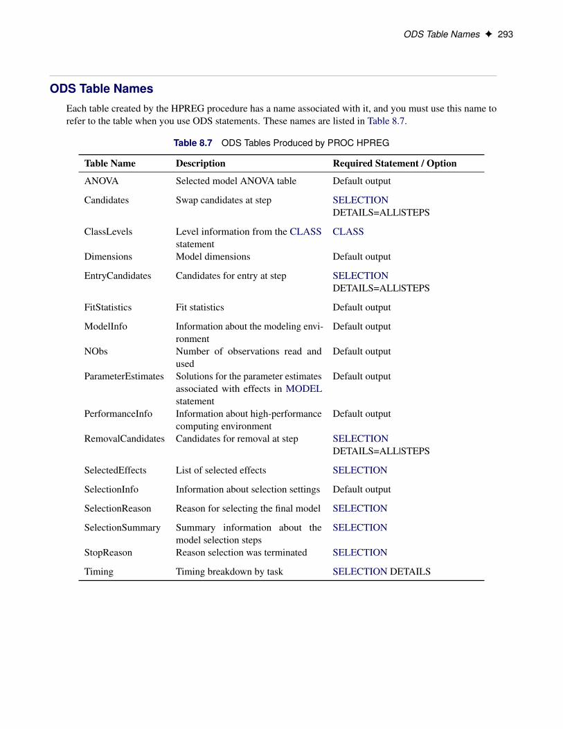
ODS Table Names F 293
ODS Table NamesEach table created by the HPREG procedure has a name associated with it, and you must use this name torefer to the table when you use ODS statements. These names are listed in Table 8.7.
Table 8.7 ODS Tables Produced by PROC HPREG
Table Name Description Required Statement / Option
ANOVA Selected model ANOVA table Default output
Candidates Swap candidates at step SELECTIONDETAILS=ALL|STEPS
ClassLevels Level information from the CLASSstatement
CLASS
Dimensions Model dimensions Default output
EntryCandidates Candidates for entry at step SELECTIONDETAILS=ALL|STEPS
FitStatistics Fit statistics Default output
ModelInfo Information about the modeling envi-ronment
Default output
NObs Number of observations read andused
Default output
ParameterEstimates Solutions for the parameter estimatesassociated with effects in MODELstatement
Default output
PerformanceInfo Information about high-performancecomputing environment
Default output
RemovalCandidates Candidates for removal at step SELECTIONDETAILS=ALL|STEPS
SelectedEffects List of selected effects SELECTION
SelectionInfo Information about selection settings Default output
SelectionReason Reason for selecting the final model SELECTION
SelectionSummary Summary information about themodel selection steps
SELECTION
StopReason Reason selection was terminated SELECTION
Timing Timing breakdown by task SELECTION DETAILS
294 F Chapter 8: The HPREG Procedure
Examples: HPREG Procedure
Example 8.1: Model Selection with ValidationThis example is based on the example “Using Validation and Cross Validation” in the documentation for theGLMSELECT procedure in the SAS/STAT User’s Guide. This example shows how you can use validationdata to monitor and control variable selection. It also demonstrates the use of split classification variables.
The following DATA step produces analysis data that contains a variable that you can use to assign observa-tions to the training, validation, and testing roles. In this case, each role has 5,000 observations.
data analysisData;drop i j c3Num;length c3$ 7;
array x{20} x1-x20;
do i=1 to 15000;do j=1 to 20;
x{j} = ranuni(1);end;
c1 = 1 + mod(i,8);c2 = ranbin(1,3,.6);
if i < 50 then do; c3 = 'tiny'; c3Num=1;end;else if i < 250 then do; c3 = 'small'; c3Num=1;end;else if i < 600 then do; c3 = 'average'; c3Num=2;end;else if i < 1200 then do; c3 = 'big'; c3Num=3;end;else do; c3 = 'huge'; c3Num=5;end;
yTrue = 10 + x1 + 2*x5 + 3*x10 + 4*x20 + 3*x1*x7 + 8*x6*x7+ 5*(c1=3)*c3Num + 8*(c1=7);
error = 5*rannor(1);
y = yTrue + error;
if mod(i,3)=1 then Role = 'TRAIN';else if mod(i,3)=2 then Role = 'VAL';else Role = 'TEST';
output;end;
run;
By construction, the true model consists of main effects x1, x5, x10, x20, and c1 and interaction effectsx1*x7, x6*x7, and c1*c3. Furthermore, you can see that only levels 3 and 7 of the classification variable c1are systematically related to the response.
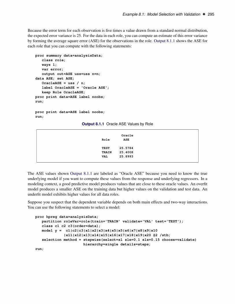
Example 8.1: Model Selection with Validation F 295
Because the error term for each observation is five times a value drawn from a standard normal distribution,the expected error variance is 25. For the data in each role, you can compute an estimate of this error varianceby forming the average square error (ASE) for the observations in the role. Output 8.1.1 shows the ASE foreach role that you can compute with the following statements:
proc summary data=analysisData;class role;ways 1;var error;output out=ASE uss=uss n=n;
data ASE; set ASE;OracleASE = uss / n;label OracleASE = 'Oracle ASE';keep Role OracleASE;
proc print data=ASE label noobs;run;
proc print data=ASE label noobs;run;
Output 8.1.1 Oracle ASE Values by Role
OracleRole ASE
TEST 25.5784TRAIN 25.4008VAL 25.8993
The ASE values shown Output 8.1.1 are labeled as “Oracle ASE” because you need to know the trueunderlying model if you want to compute these values from the response and underlying regressors. In amodeling context, a good predictive model produces values that are close to these oracle values. An overfitmodel produces a smaller ASE on the training data but higher values on the validation and test data. Anunderfit model exhibits higher values for all data roles.
Suppose you suspect that the dependent variable depends on both main effects and two-way interactions.You can use the following statements to select a model:
proc hpreg data=analysisData;partition roleVar=role(train='TRAIN' validate='VAL' test='TEST');class c1 c2 c3(order=data);model y = c1|c2|c3|x1|x2|x3|x4|x5|x5|x6|x7|x8|x9|x10
|x11|x12|x13|x14|x15|x16|x17|x18|x19|x20 @2 /stb;selection method = stepwise(select=sl sle=0.1 sls=0.15 choose=validate)
hierarchy=single details=steps;run;

296 F Chapter 8: The HPREG Procedure
A PARTITION statement assigns observations to training, validation, and testing roles based on the val-ues of the input variable named role. The SELECTION statement requests STEPWISE selection basedon significance level where the SLE and SLS values are set to use the defaults of PROC REG. TheCHOOSE=VALIDATE option selects the model that yields the smallest ASE value on the validation data.
The “Number Of Observation” table in Output 8.1.2 confirms that there are 5,000 observations for each datarole. The “Dimensions” table shows that the selection is from 278 effects with a total of 661 parameters.
Output 8.1.2 Number of Observations, Class Levels, and Dimensions
The HPREG Procedure
Number of Observations Read 15000Number of Observations Used 15000Number of Observations Used for Training 5000Number of Observations Used for Validation 5000Number of Observations Used for Testing 5000
Class Level Information
Class Levels Values
c1 8 1 2 3 4 5 6 7 8c2 4 0 1 2 3c3 5 tiny small average big huge
Dimensions
Number of Effects 278Number of Parameters 661
Output 8.1.3 shows the “Selection Summary” table. You see that 18 steps are done, at which point all effectsin the model are significant at the SLS value of 0.15 and all the remaining effects if added individuallywould not be significant at the SLE significance level of 0.1. However, because you have specified theCHOOSE=VALIDATE option, the model at step 18 is not used as the selected model. Instead the modelat step 10 (where the validation ASE achieves a local minimum value) is selected. The “Stop Reason,”“Selection Reason,” and “Selected Effects” in Output 8.1.4 provide this information.

Example 8.1: Model Selection with Validation F 297
Output 8.1.3 Selection Summary
The HPREG Procedure
Selection Summary
Effect Number Validation pStep Entered Effects In ASE Value
0 Intercept 1 98.3895 1.0000------------------------------------------------------------
1 c1 2 34.8572 <.00012 x7 3 32.5531 <.00013 x6 4 31.0646 <.00014 x20 5 29.7078 <.00015 x6*x7 6 29.2210 <.00016 x10 7 28.6683 <.00017 x1 8 28.3250 <.00018 x5 9 27.9766 <.00019 c3 10 27.8288 <.0001
10 c1*c3 11 25.9701* <.000111 x10*c1 12 26.0696 0.010912 x4 13 26.1594 0.012813 x4*x10 14 26.1814 0.003514 x20*c1 15 26.3294 0.015615 x1*c3 16 26.3945 0.024416 x1*x7 17 26.3632 0.027017 x7*x10 18 26.4120 0.031318 x1*x20 19 26.4330 0.0871
* Optimal Value of Criterion
Output 8.1.4 Stopping and Selection Reasons
Selection stopped because all candidates for removal are significant at the 0.15level and no candidate for entry is significant at the 0.1 level.
The model at step 10 is selected where Validation ASE is 25.9701.
Selected Effects: Intercept c1 c3 c1*c3 x1 x5 x6 x7 x6*x7 x10 x20
You can see that the selected effects include all the main effects in the true model and two of the three trueinteraction terms. Furthermore, the selected model does not include any variables that are not in the truemodel. Note that these statements are not true of the larger model at the final step of the selection process.
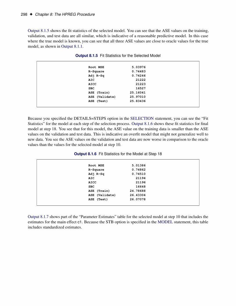
298 F Chapter 8: The HPREG Procedure
Output 8.1.5 shows the fit statistics of the selected model. You can see that the ASE values on the training,validation, and test data are all similar, which is indicative of a reasonable predictive model. In this casewhere the true model is known, you can see that all three ASE values are close to oracle values for the truemodel, as shown in Output 8.1.1.
Output 8.1.5 Fit Statistics for the Selected Model
Root MSE 5.03976R-Square 0.74483Adj R-Sq 0.74246AIC 21222AICC 21223SBC 16527ASE (Train) 25.16041ASE (Validate) 25.97010ASE (Test) 25.83436
Because you specified the DETAILS=STEPS option in the SELECTION statement, you can see the “FitStatistics” for the model at each step of the selection process. Output 8.1.6 shows these fit statistics for finalmodel at step 18. You see that for this model, the ASE value on the training data is smaller than the ASEvalues on the validation and test data. This is indicative an overfit model that might not generalize well tonew data. You see the ASE values on the validation and test data are now worse in comparison to the oraclevalues than the values for the selected model at step 10.
Output 8.1.6 Fit Statistics for the Model at Step 18
Root MSE 5.01386R-Square 0.74862Adj R-Sq 0.74510AIC 21194AICC 21196SBC 16648ASE (Train) 24.78688ASE (Validate) 26.43304ASE (Test) 26.07078
Output 8.1.7 shows part of the “Parameter Estimates” table for the selected model at step 10 that includes theestimates for the main effect c1. Because the STB option is specified in the MODEL statement, this tableincludes standardized estimates.

Example 8.1: Model Selection with Validation F 299
Output 8.1.7 Part of the Parameter Estimates Table for the Selected Model
Parameter Estimates
Standardized StandardParameter DF Estimate Estimate Error t Value Pr > |t|
Intercept 1 9.479114 0 0.422843 22.42 <.0001c1 1 1 0.279417 0.009306 0.297405 0.94 0.3475c1 2 1 0.615589 0.020502 0.297332 2.07 0.0385c1 3 1 25.678601 0.855233 0.297280 86.38 <.0001c1 4 1 0.420360 0.014000 0.297283 1.41 0.1574c1 5 1 0.473986 0.015786 0.297265 1.59 0.1109c1 6 1 0.394044 0.013124 0.297299 1.33 0.1851c1 7 1 8.469793 0.282089 0.297345 28.48 <.0001c1 8 0 0 0 . . .
The magnitudes of the standardized estimates and the t statistics of the parameters of the effect c1 reveal thatonly levels 3 and 7 of this effect contribute appreciably to the model. This suggests that a more parsimoniousmodel with similar or better predictive power might be obtained if parameters that correspond to the levelsof c1 can enter or leave the model independently. You request this with the SPLIT option in the CLASSstatement as shown in the following statements:
proc hpreg data=analysisData;partition roleVar=role(train='TRAIN' validate='VAL' test='TEST');class c1(split) c2 c3(order=data);model y = c1|c2|c3|x1|x2|x3|x4|x5|x5|x6|x7|x8|x9|x10
|x11|x12|x13|x14|x15|x16|x17|x18|x19|x20 @2 /stb;selection method = stepwise(select=sl sle=0.1 sls=0.15 choose=validate)
hierarchy=single details=steps;run;
Output 8.1.8 shows the “Dimensions” table. You can see that because the columns in the design matrix thatcorrespond to levels of c1 are treated as separate effects, the selection is now from 439 effects, even thoughthe number of parameters is unchanged.
Output 8.1.8 Dimensions with c1 Split
The HPREG Procedure
Dimensions
Number of Effects 278Number of Effects after Splits 439Number of Parameters 661
300 F Chapter 8: The HPREG Procedure
Output 8.1.9 shows the selected effects. You can see that as anticipated the selected model now depends ononly levels 3 and 7 of c1.
Output 8.1.9 Selected Effects with c1 Split
Selected Effects: Intercept c1_3 c1_7 c3 c1_3*c3 x1 x5 x6 x7 x6*x7 x10 x20
Finally, the fit statistics for the selected model are shown Output 8.1.10.
Output 8.1.10 Fit Statistics for the Selected Model with c1 Split
Root MSE 5.04060R-Square 0.74325Adj R-Sq 0.74238AIC 21195AICC 21195SBC 16311ASE (Train) 25.31622ASE (Validate) 25.98055ASE (Test) 25.76059
If you compare the ASE values for this model in Output 8.1.10 with the oracle values in Output 8.1.1 andthe values for the model without splitting c1 in Output 8.1.5, you see that this more parsimonious modelproduces the best predictive performance on the test data of all the models considered in this example.
Example 8.2: Backward Selection in Single-Machine and Distributed ModesThis example shows how you can run PROC HPREG in single-machine and distributed modes. See thesection “Processing Modes” on page 6 in Chapter 2, “Shared Concepts and Topics,” for details about theexecution modes of SAS High-Performance Statistics procedures. The focus of this example is to simplyshow how you can switch the modes of execution of PROC HPREG, rather than on any statistical features ofthe procedure. The following DATA step generates the data for this example. The response y depends on 20of the 1,000 regressors.
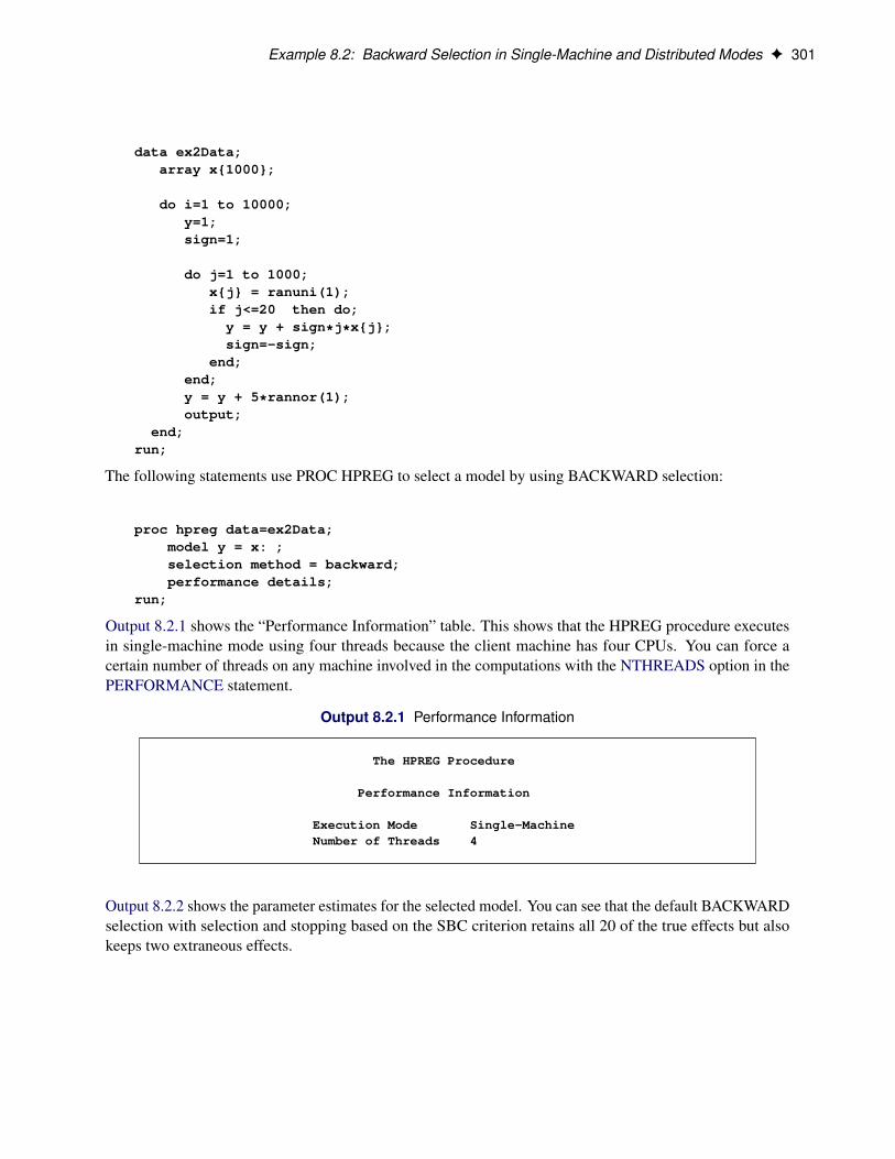
Example 8.2: Backward Selection in Single-Machine and Distributed Modes F 301
data ex2Data;array x{1000};
do i=1 to 10000;y=1;sign=1;
do j=1 to 1000;x{j} = ranuni(1);if j<=20 then do;
y = y + sign*j*x{j};sign=-sign;
end;end;y = y + 5*rannor(1);output;
end;run;
The following statements use PROC HPREG to select a model by using BACKWARD selection:
proc hpreg data=ex2Data;model y = x: ;selection method = backward;performance details;
run;
Output 8.2.1 shows the “Performance Information” table. This shows that the HPREG procedure executesin single-machine mode using four threads because the client machine has four CPUs. You can force acertain number of threads on any machine involved in the computations with the NTHREADS option in thePERFORMANCE statement.
Output 8.2.1 Performance Information
The HPREG Procedure
Performance Information
Execution Mode Single-MachineNumber of Threads 4
Output 8.2.2 shows the parameter estimates for the selected model. You can see that the default BACKWARDselection with selection and stopping based on the SBC criterion retains all 20 of the true effects but alsokeeps two extraneous effects.

302 F Chapter 8: The HPREG Procedure
Output 8.2.2 Parameter Estimates for the Selected Model
Parameter Estimates
StandardParameter DF Estimate Error t Value Pr > |t|
Intercept 1 1.506615 0.419811 3.59 0.0003x1 1 1.054402 0.176930 5.96 <.0001x2 1 -1.996080 0.176967 -11.28 <.0001x3 1 3.293331 0.177032 18.60 <.0001x4 1 -3.741273 0.176349 -21.22 <.0001x5 1 4.908310 0.176047 27.88 <.0001x6 1 -5.772356 0.176642 -32.68 <.0001x7 1 7.398822 0.175792 42.09 <.0001x8 1 -7.958471 0.176281 -45.15 <.0001x9 1 8.899407 0.177624 50.10 <.0001x10 1 -9.687667 0.176431 -54.91 <.0001x11 1 11.083373 0.175195 63.26 <.0001x12 1 -12.046504 0.176324 -68.32 <.0001x13 1 13.009052 0.176967 73.51 <.0001x14 1 -14.456393 0.175968 -82.15 <.0001x15 1 14.928731 0.174868 85.37 <.0001x16 1 -15.762907 0.177651 -88.73 <.0001x17 1 16.842889 0.177037 95.14 <.0001x18 1 -18.468844 0.176502 -104.64 <.0001x19 1 18.810193 0.176616 106.50 <.0001x20 1 -20.212291 0.176325 -114.63 <.0001x87 1 -0.542384 0.176293 -3.08 0.0021x362 1 -0.560999 0.176594 -3.18 0.0015
Output 8.2.3 shows timing information for the PROC HPREG run. This table is produced when you specifythe DETAILS option in the PERFORMANCE statement. You can see that, in this case, the majority of timeis spent forming the crossproducts matrix for the model that contains all the regressors.
Output 8.2.3 Timing
Procedure Task Timing
Task Seconds Percent
Reading and Levelizing Data 0.69 4.18%Loading Design Matrix 0.31 1.90%Computing Moments 0.08 0.48%Computing Cross Products Matrix 12.62 76.98%Performing Model Selection 2.70 16.46%
You can switch to running PROC HPREG in distributed mode by specifying valid values for the NODES=,INSTALL=, and HOST= options in the PERFORMANCE statement. An alternative to specifying theINSTALL= and HOST= options in the PERFORMANCE statement is to set appropriate values for theGRIDHOST and GRIDINSTALLLOC environment variables by using OPTIONS SET commands. See the

Example 8.2: Backward Selection in Single-Machine and Distributed Modes F 303
section “Processing Modes” on page 6 in Chapter 2, “Shared Concepts and Topics,” for details about settingthese options or environment variables.
The following statements provide an example. To run these statements successfully, you need to set themacro variables GRIDHOST and GRIDINSTALLLOC to resolve to appropriate values, or you can replace thereferences to macro variables with appropriate values.
proc hpreg data=ex2Data;model y = x: ;selection method = backward;performance details nodes = 10
host="&GRIDHOST" install="&GRIDINSTALLLOC";run;
The execution mode in the “Performance Information” table shown in Output 8.2.4 indicates that thecalculations were performed in a distributed environment that uses 10 nodes, each of which uses eightthreads.
Output 8.2.4 Performance Information in Distributed Mode
Performance Information
Host Node << your grid host >>Install Location << your grid install location >>Execution Mode DistributedGrid Mode SymmetricNumber of Compute Nodes 10Number of Threads per Node 8
Another indication of distributed execution is the following message issued by all High-Performance Analyticsprocedures in the SAS Log:
NOTE: The HPREG procedure is executing in the distributedcomputing environment with 10 worker nodes.
Output 8.2.5 shows timing information for this distributed run of the HPREG procedure. In contrast to thesingle-machine mode (where forming the crossproducts matrix dominated the time spent), the majority oftime in distributed mode is spent performing the model selection.
Output 8.2.5 Timing
Procedure Task Timing
Task Seconds Percent
Distributing Data 0.93 18.68%Reading and Levelizing Data 0.03 0.66%Loading Design Matrix 0.01 0.22%Computing Moments 0.01 0.14%Computing Cross Products Matrix 1.19 23.82%Performing Model Selection 2.48 49.60%Waiting on Client 0.34 6.88%
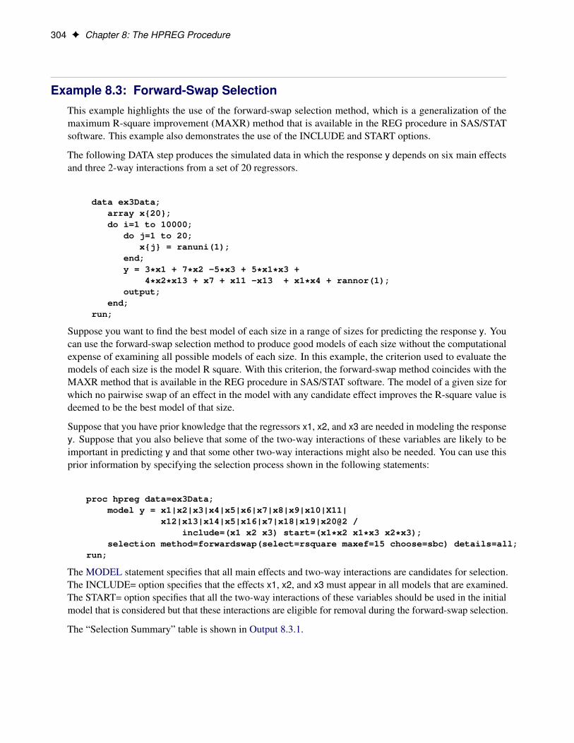
304 F Chapter 8: The HPREG Procedure
Example 8.3: Forward-Swap SelectionThis example highlights the use of the forward-swap selection method, which is a generalization of themaximum R-square improvement (MAXR) method that is available in the REG procedure in SAS/STATsoftware. This example also demonstrates the use of the INCLUDE and START options.
The following DATA step produces the simulated data in which the response y depends on six main effectsand three 2-way interactions from a set of 20 regressors.
data ex3Data;array x{20};do i=1 to 10000;
do j=1 to 20;x{j} = ranuni(1);
end;y = 3*x1 + 7*x2 -5*x3 + 5*x1*x3 +
4*x2*x13 + x7 + x11 -x13 + x1*x4 + rannor(1);output;
end;run;
Suppose you want to find the best model of each size in a range of sizes for predicting the response y. Youcan use the forward-swap selection method to produce good models of each size without the computationalexpense of examining all possible models of each size. In this example, the criterion used to evaluate themodels of each size is the model R square. With this criterion, the forward-swap method coincides with theMAXR method that is available in the REG procedure in SAS/STAT software. The model of a given size forwhich no pairwise swap of an effect in the model with any candidate effect improves the R-square value isdeemed to be the best model of that size.
Suppose that you have prior knowledge that the regressors x1, x2, and x3 are needed in modeling the responsey. Suppose that you also believe that some of the two-way interactions of these variables are likely to beimportant in predicting y and that some other two-way interactions might also be needed. You can use thisprior information by specifying the selection process shown in the following statements:
proc hpreg data=ex3Data;model y = x1|x2|x3|x4|x5|x6|x7|x8|x9|x10|X11|
x12|x13|x14|x5|x16|x7|x18|x19|x20@2 /include=(x1 x2 x3) start=(x1*x2 x1*x3 x2*x3);
selection method=forwardswap(select=rsquare maxef=15 choose=sbc) details=all;run;
The MODEL statement specifies that all main effects and two-way interactions are candidates for selection.The INCLUDE= option specifies that the effects x1, x2, and x3 must appear in all models that are examined.The START= option specifies that all the two-way interactions of these variables should be used in the initialmodel that is considered but that these interactions are eligible for removal during the forward-swap selection.
The “Selection Summary” table is shown in Output 8.3.1.
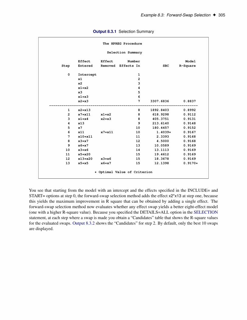
Example 8.3: Forward-Swap Selection F 305
Output 8.3.1 Selection Summary
The HPREG Procedure
Selection Summary
Effect Effect Number ModelStep Entered Removed Effects In SBC R-Square
0 Intercept 1x1 2x2 3x1*x2 4x3 5x1*x3 6x2*x3 7 3307.6836 0.8837
------------------------------------------------------------------------1 x2*x13 8 1892.8403 0.89922 x7*x11 x1*x2 8 618.9298 0.91123 x1*x4 x2*x3 8 405.3751 0.91314 x13 9 213.6140 0.91485 x7 10 180.4457 0.91526 x11 x7*x11 10 1.4039* 0.91677 x10*x11 11 2.3393 0.91688 x3*x7 12 4.5000 0.91689 x6*x7 13 10.0589 0.9169
10 x3*x6 14 13.1113 0.916911 x5*x20 15 19.4612 0.916912 x13*x20 x3*x6 15 18.3678 0.916913 x5*x5 x6*x7 15 12.1398 0.9170*
* Optimal Value of Criterion
You see that starting from the model with an intercept and the effects specified in the INCLUDE= andSTART= options at step 0, the forward-swap selection method adds the effect x2*x13 at step one, becausethis yields the maximum improvement in R square that can be obtained by adding a single effect. Theforward-swap selection method now evaluates whether any effect swap yields a better eight-effect model(one with a higher R-square value). Because you specified the DETAILS=ALL option in the SELECTIONstatement, at each step where a swap is made you obtain a “Candidates” table that shows the R-square valuesfor the evaluated swaps. Output 8.3.2 shows the “Candidates” for step 2. By default, only the best 10 swapsare displayed.

306 F Chapter 8: The HPREG Procedure
Output 8.3.2 Swap Candidates at Step 2
Best 10 Candidates
Effect EffectRank Dropped Added R-Square
1 x1*x2 x7*x11 0.91122 x2*x3 x7*x11 0.91123 x1*x2 x7 0.90654 x2*x3 x7 0.90655 x1*x2 x7*x7 0.90606 x2*x3 x7*x7 0.90607 x1*x2 x4*x7 0.90608 x2*x3 x4*x7 0.90609 x1*x2 x11 0.905810 x2*x3 x11 0.9058
You see that the best swap adds x7*x11 and drops x1*x2. This yields an eight-effect model whose R-squarevalue (0.9112) is larger than the R-square value (0.8992) of the eight-effect model at step 1. Hence thisswap is made at step 2. At step 3, an even better eight-effect model than the model at step 2 is obtained bydropping x2*x3 and adding x1*x4. No additional swap improves the R-square value, and so the model at step3 is deemed to be the best eight-effect model. Although this is the best eight-effect model that can be foundby this method given the starting model, it is not guaranteed that this model that has the highest R-squarevalue among all possible models that consist of seven effects and an intercept.
Because the DETAILS=ALL option is specified in the SELECTION statement, details for the model at eachstep of the selection process are displayed. Output 8.3.3 provides details of the model at step 3.
Output 8.3.3 Model Details at Step 3
Analysis of Variance
Sum of MeanSource DF Squares Square F Value Pr > F
Model 7 108630 15519 15000.3 <.0001Error 9992 10337 1.03455Corrected Total 9999 118967
Root MSE 1.01713R-Square 0.91311Adj R-Sq 0.91305AIC 10350AICC 10350SBC 405.37511ASE 1.03373

References F 307
Output 8.3.3 continued
Parameter Estimates
StandardParameter DF Estimate Error t Value Pr > |t|
Intercept 1 0.012095 0.045712 0.26 0.7913x1 1 3.087078 0.076390 40.41 <.0001x2 1 7.775180 0.046815 166.08 <.0001x3 1 -4.957140 0.070995 -69.82 <.0001x1*x3 1 4.910115 0.122503 40.08 <.0001x1*x4 1 0.890436 0.060523 14.71 <.0001x7*x11 1 1.708469 0.045939 37.19 <.0001x2*x13 1 2.584078 0.061506 42.01 <.0001
The forward-swap method continues to find the best nine-effect model, best 10-effect model, and so on until itobtains the best 15-effect model. At this point the selection terminates because you specified the MAXEF=15option in the SELECTION statement. The R-square value increases at each step of the selection process.However, because you specified the CHOOSE=SBC criterion in the SELECTION statement, the final modelselected is the model at step 6.
References
Akaike, H. (1969), “Fitting Autoregressive Models for Prediction,” Annals of the Institute of StatisticalMathematics, 21, 243–247.
Burnham, K. P. and Anderson, D. R. (2002), Model Selection and Multimodel Inference, 2nd Edition, NewYork: Springer-Verlag.
Collier Books (1987), The 1987 Baseball Encyclopedia Update, New York: Macmillan.
Darlington, R. B. (1968), “Multiple Regression in Psychological Research and Practice,” PsychologicalBulletin, 69, 161–182.
Draper, N. R., Guttman, I., and Kanemasu, H. (1971), “The Distribution of Certain Regression Statistics,”Biometrika, 58, 295–298.
Harrell, F. E. (2001), Regression Modeling Strategies, New York: Springer-Verlag.
Hastie, T. J., Tibshirani, R. J., and Friedman, J. H. (2001), The Elements of Statistical Learning, New York:Springer-Verlag.
Hocking, R. R. (1976), “The Analysis and Selection of Variables in a Linear Regression,” Biometrics, 32,1–50.
Hurvich, C. M. and Tsai, C.-L. (1989), “Regression and Time Series Model Selection in Small Samples,”Biometrika, 76, 297–307.

308 F Chapter 8: The HPREG Procedure
Judge, G. G., Griffiths, W. E., Hill, R. C., Lütkepohl, H., and Lee, T.-C. (1985), The Theory and Practice ofEconometrics, 2nd Edition, New York: John Wiley & Sons.
Mallows, C. L. (1973), “Some Comments on Cp,” Technometrics, 15, 661–675.
Schwarz, G. (1978), “Estimating the Dimension of a Model,” Annals of Statistics, 6, 461–464.
Time Inc. (1987), “What They Make,” Sports Illustrated, April, 54–81.

Chapter 9
The HPSPLIT Procedure
ContentsOverview: HPSPLIT Procedure . . . . . . . . . . . . . . . . . . . . . . . . . . . . . . . . 310
PROC HPSPLIT Features . . . . . . . . . . . . . . . . . . . . . . . . . . . . . . . . 310Getting Started: HPSPLIT Procedure . . . . . . . . . . . . . . . . . . . . . . . . . . . . . 311Syntax: HPSPLIT Procedure . . . . . . . . . . . . . . . . . . . . . . . . . . . . . . . . . . 314
PROC HPSPLIT Statement . . . . . . . . . . . . . . . . . . . . . . . . . . . . . . . 314CODE Statement . . . . . . . . . . . . . . . . . . . . . . . . . . . . . . . . . . . . . 316CRITERION Statement . . . . . . . . . . . . . . . . . . . . . . . . . . . . . . . . . 316ID Statement . . . . . . . . . . . . . . . . . . . . . . . . . . . . . . . . . . . . . . . 317INPUT Statement . . . . . . . . . . . . . . . . . . . . . . . . . . . . . . . . . . . . 317OUTPUT Statement . . . . . . . . . . . . . . . . . . . . . . . . . . . . . . . . . . . 318PARTITION Statement . . . . . . . . . . . . . . . . . . . . . . . . . . . . . . . . . 319PERFORMANCE Statement . . . . . . . . . . . . . . . . . . . . . . . . . . . . . . 320PRUNE Statement . . . . . . . . . . . . . . . . . . . . . . . . . . . . . . . . . . . . 320RULES Statement . . . . . . . . . . . . . . . . . . . . . . . . . . . . . . . . . . . . 322SCORE Statement . . . . . . . . . . . . . . . . . . . . . . . . . . . . . . . . . . . . 322TARGET Statement . . . . . . . . . . . . . . . . . . . . . . . . . . . . . . . . . . . 322
Details: HPSPLIT Procedure . . . . . . . . . . . . . . . . . . . . . . . . . . . . . . . . . . 322Building a Tree . . . . . . . . . . . . . . . . . . . . . . . . . . . . . . . . . . . . . . 322Interval Input Binning Details . . . . . . . . . . . . . . . . . . . . . . . . . . . . . . 323Input Variable Splitting and Selection . . . . . . . . . . . . . . . . . . . . . . . . . . 324Pruning . . . . . . . . . . . . . . . . . . . . . . . . . . . . . . . . . . . . . . . . . . 325Memory Considerations . . . . . . . . . . . . . . . . . . . . . . . . . . . . . . . . . 326Handling Missing Values . . . . . . . . . . . . . . . . . . . . . . . . . . . . . . . . 326Handling Unknown Levels in Scoring . . . . . . . . . . . . . . . . . . . . . . . . . . 327Splitting Criteria . . . . . . . . . . . . . . . . . . . . . . . . . . . . . . . . . . . . . 327Pruning Criteria . . . . . . . . . . . . . . . . . . . . . . . . . . . . . . . . . . . . . 328Subtree Statistics . . . . . . . . . . . . . . . . . . . . . . . . . . . . . . . . . . . . . 329Variable Importance . . . . . . . . . . . . . . . . . . . . . . . . . . . . . . . . . . . 335Outputs . . . . . . . . . . . . . . . . . . . . . . . . . . . . . . . . . . . . . . . . . . 336
Examples: HPSPLIT Procedure . . . . . . . . . . . . . . . . . . . . . . . . . . . . . . . . 338Example 9.1: Creating an English Rules Description of a Tree . . . . . . . . . . . . . 338Example 9.2: Assessing Variable Importance . . . . . . . . . . . . . . . . . . . . . . 340
References . . . . . . . . . . . . . . . . . . . . . . . . . . . . . . . . . . . . . . . . . . . 342
310 F Chapter 9: The HPSPLIT Procedure
Overview: HPSPLIT ProcedureThe HPSPLIT procedure is a high-performance utility procedure that creates a decision tree model and savesresults in output data sets and files for use in SAS Enterprise Miner.
PROC HPSPLIT runs in either single-machine mode or distributed mode.
NOTE: Distributed mode requires SAS High-Performance Statistics.
PROC HPSPLIT FeaturesThe main features of the HPSPLIT procedure are as follows:
• Model creation
– supports interval and nominal inputs
– supports nominal targets
– provides the entropy, Gini, and FastCHAID methods for tree growth
– provides multiple statistical metrics for tree pruning
– provides C4.5-style pruning
– partitions the input data set into training and validation sets
• Score output data set
– saves scored results for the training data
– provides predicted levels and posterior probabilities
• Score code file
– saves SAS DATA step code, which can be used for scoring new data with the tree model
• Rules file
– saves English rules that describe the leaves of the tree
• Node output data set
– saves statistics and descriptive information for the nodes in the tree
• Variable importance output data set
– saves the importance of the input variables in creating the pruned decision tree
– provides variable importance for the validation set
• Subtree monitoring output data sets
– save statistical metrics for each subtree that is created during growth
– save statistical metrics for each subtree that is created during pruning
Getting Started: HPSPLIT Procedure F 311
Because the HPSPLIT procedure is a high-performance analytical procedure, it also does the following:
• enables you to run in distributed mode on a cluster of machines that distribute the data and thecomputations
• enables you to run in single-machine mode on the server where SAS is installed
• exploits all of the available cores and concurrent threads, regardless of execution mode.
For more information, see the section “Processing Modes” on page 6 in Chapter 2, “Shared Concepts andTopics.”
Getting Started: HPSPLIT ProcedureDecision trees are commonly used in banking to predict default in mortgage applications. The data set HMEQ,which is in the sample library, contains observations for 5,960 mortgage applicants. A variable named BADindicates whether the applicant paid or defaulted on the loan.
This example uses HMEQ to build a tree model that is used to score the data and can be used to score data onnew applicants. Table 9.1 describes the variables in HMEQ.
Table 9.1 Variables in the Home Equity (HMEQ) Data Set
Variable Role Level Description
BAD Target Binary 1 = applicant defaulted on the loan or is seriously delinquent0 = applicant paid the loan
CLAGE Input Interval Age of oldest credit line in monthsCLNO Input Interval Number of credit linesDEBTINC Input Interval Debt-to-income ratioDELINQ Input Interval Number of delinquent credit linesDEROG Input Interval Number of major derogatory reportsJOB Input Nominal Occupational categoryLOAN Input Interval Requested loan amountMORTDUE Input Interval Amount due on existing mortgageNINQ Input Interval Number of recent credit inquiriesREASON Input Binary DebtCon = debt consolidation
HomeImp = home improvementVALUE Input Interval Value of current propertyYOJ Input Interval Years at present job
Figure 9.1 shows a partial listing of HMEQ.
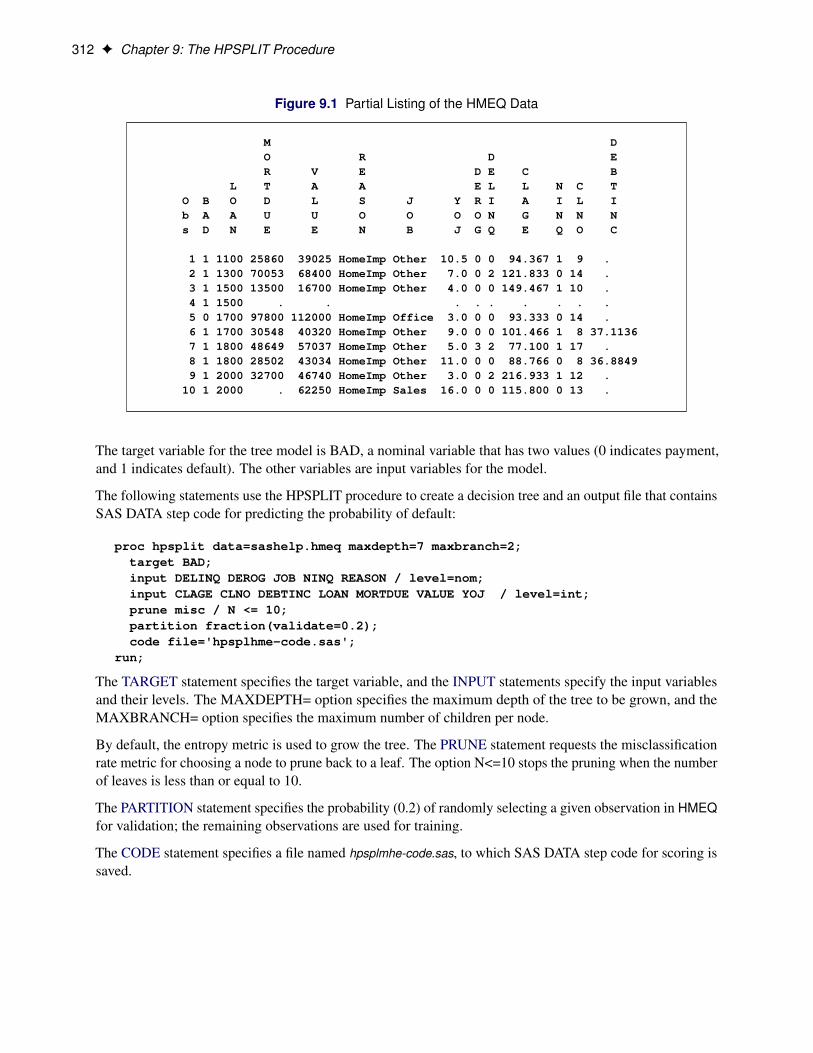
312 F Chapter 9: The HPSPLIT Procedure
Figure 9.1 Partial Listing of the HMEQ Data
M DO R D ER V E D E C B
L T A A E L L N C TO B O D L S J Y R I A I L Ib A A U U O O O O N G N N Ns D N E E N B J G Q E Q O C
1 1 1100 25860 39025 HomeImp Other 10.5 0 0 94.367 1 9 .2 1 1300 70053 68400 HomeImp Other 7.0 0 2 121.833 0 14 .3 1 1500 13500 16700 HomeImp Other 4.0 0 0 149.467 1 10 .4 1 1500 . . . . . . . . .5 0 1700 97800 112000 HomeImp Office 3.0 0 0 93.333 0 14 .6 1 1700 30548 40320 HomeImp Other 9.0 0 0 101.466 1 8 37.11367 1 1800 48649 57037 HomeImp Other 5.0 3 2 77.100 1 17 .8 1 1800 28502 43034 HomeImp Other 11.0 0 0 88.766 0 8 36.88499 1 2000 32700 46740 HomeImp Other 3.0 0 2 216.933 1 12 .
10 1 2000 . 62250 HomeImp Sales 16.0 0 0 115.800 0 13 .
The target variable for the tree model is BAD, a nominal variable that has two values (0 indicates payment,and 1 indicates default). The other variables are input variables for the model.
The following statements use the HPSPLIT procedure to create a decision tree and an output file that containsSAS DATA step code for predicting the probability of default:
proc hpsplit data=sashelp.hmeq maxdepth=7 maxbranch=2;target BAD;input DELINQ DEROG JOB NINQ REASON / level=nom;input CLAGE CLNO DEBTINC LOAN MORTDUE VALUE YOJ / level=int;prune misc / N <= 10;partition fraction(validate=0.2);code file='hpsplhme-code.sas';
run;
The TARGET statement specifies the target variable, and the INPUT statements specify the input variablesand their levels. The MAXDEPTH= option specifies the maximum depth of the tree to be grown, and theMAXBRANCH= option specifies the maximum number of children per node.
By default, the entropy metric is used to grow the tree. The PRUNE statement requests the misclassificationrate metric for choosing a node to prune back to a leaf. The option N<=10 stops the pruning when the numberof leaves is less than or equal to 10.
The PARTITION statement specifies the probability (0.2) of randomly selecting a given observation in HMEQfor validation; the remaining observations are used for training.
The CODE statement specifies a file named hpsplmhe-code.sas, to which SAS DATA step code for scoring issaved.

Getting Started: HPSPLIT Procedure F 313
The following statements score the data in HMEQ and save the results in a SAS data set named SCORED.
data scored;set sashelp.hmeq;%include 'hpsplhme-code.sas';
run;
A partial listing of SCORED is shown in Figure 9.2.
Figure 9.2 Partial Listing of the Scored HMEQ Data
Obs BAD LOAN MORTDUE VALUE REASON JOB YOJ DEROG DELINQ CLAGE NINQ
1 1 1100 25860 39025 HomeImp Other 10.5 0 0 94.367 12 1 1300 70053 68400 HomeImp Other 7.0 0 2 121.833 03 1 1500 13500 16700 HomeImp Other 4.0 0 0 149.467 14 1 1500 . . . . . . .5 0 1700 97800 112000 HomeImp Office 3.0 0 0 93.333 06 1 1700 30548 40320 HomeImp Other 9.0 0 0 101.466 17 1 1800 48649 57037 HomeImp Other 5.0 3 2 77.100 18 1 1800 28502 43034 HomeImp Other 11.0 0 0 88.766 09 1 2000 32700 46740 HomeImp Other 3.0 0 2 216.933 1
10 1 2000 . 62250 HomeImp Sales 16.0 0 0 115.800 0
Obs CLNO DEBTINC _NODE_ _LEAF_ _WARN_ P_BAD1 P_BAD0 V_BAD1 V_BAD0
1 9 . 16 7 0.17391 0.82609 0.18808 0.811922 14 . 13 6 0.29969 0.70031 0.32450 0.675503 10 . 16 7 0.17391 0.82609 0.18808 0.811924 . . 16 7 0.17391 0.82609 0.18808 0.811925 14 . 16 7 0.17391 0.82609 0.18808 0.811926 8 37.1136 16 7 0.17391 0.82609 0.18808 0.811927 17 . 6 2 0.93939 0.06061 0.87500 0.125008 8 36.8849 16 7 0.17391 0.82609 0.18808 0.811929 12 . 13 6 0.29969 0.70031 0.32450 0.67550
10 13 . 16 7 0.17391 0.82609 0.18808 0.81192
The data set contains the original variables and new variables that are created by the score statements. Thevariable P_BAD1 is the proportion of training observations at this leaf that have BAD=1, and this variable canbe interpreted as the probability of default. The variable V_BAD1 is the proportion of validation observationsat this leaf that have BAD=1. The other new variables are described in the section “Outputs” on page 336
The preceding statements can be used to score new data by including the new data set in place of HMEQ. Thenew data set must contain the same variables as the data that are used to build the tree model.
314 F Chapter 9: The HPSPLIT Procedure
Syntax: HPSPLIT ProcedureThe following statements and options are available in the HPSPLIT procedure:
PROC HPSPLIT < options > ;CODE FILE=filename ;CRITERION criterion < / options > ;ID variables ;INPUT variables < / option > ;OUTPUT < output-options > < / subtreestat-option > ;PARTITION < partition-options > ;PERFORMANCE performance-options ;PRUNE < prune-options > ;RULES FILE=filename ;SCORE OUT=SAS-data-set ;TARGET variable < / option > ;
The PROC HPSPLIT statement, the TARGET statement, and the INPUT statement are required. It isrecommended that you use at least one of the following statements: OUTPUT, RULES, or CODE.
The following sections describe the PROC HPSPLIT statement and then describe the other statements inalphabetical order.
PROC HPSPLIT StatementPROC HPSPLIT < options > ;
The PROC HPSPLIT statement invokes the procedure. Table 9.2 summarizes the options in the PROCHPSPLIT statement.
Table 9.2 PROC HPSPLIT Statement Options
Option Description
Basic OptionsDATA= Specifies the input data setEVENT= Specifies the formatted value of the target eventINTERVALBINS= Specifies the number of bins for interval variables
Splitting OptionsLEAFSIZE= Specifies the minimum number of observations per leafMAXBRANCH= Specifies the maximum leaves per nodeMAXDEPTH= Specifies the maximum tree depthMINCATSIZE= Specifies the number of observations per level to consider a level
for splitting
FastCHAID OptionsALPHA= Specifies the maximum p-value for a split to be consideredBONFERRNOI Enables the Bonferroni adjustment to after-split p-valuesMINDIST= Specifies the minimum Kolmogorov-Smirnov distance

PROC HPSPLIT Statement F 315
DATA=SAS-data-setnames the input SAS data set to be used by PROC HPSPLIT. The default is the most recently createddata set.
If the procedure executes in distributed mode, the input data are distributed to memory on the appliancenodes and analyzed in parallel, unless the data are already distributed in the appliance database. In thatcase the procedure reads the data alongside the distributed database. See the section “Processing Modes”on page 6 about the various execution modes and the section “Alongside-the-Database Execution” onpage 13 about the alongside-the-database model. Both sections are in Chapter 2, “Shared Conceptsand Topics.”
EVENT=valuespecifies a formatted value of the target level variable to use for sorting nominal input levels whenyou use the FastCHAID criterion or when PROC HPSPLIT uses the fastest splitting category. Ties arebroken in internal order. For example, if you are looking for defects in a data set where a target valueof ‘D’ indicates a defect, specify EVENT=‘D’.
See section “Input Variable Splitting and Selection” on page 324 for details on splitting categories andthe FastCHAID criterion.
The default is the first level of the target as specified by the ORDER= option in the TARGET statement.
INTERVALBINS=numberspecifies the number of bins for interval variables. For more information about interval variablebinning, see the section “Details: HPSPLIT Procedure” on page 322.
The default is INTERVALBINS=100.
LEAFSIZE=numberspecifies the minimum number of observations that a split must contain in the training data set in orderfor the split to be considered.
The default is LEAFSIZE=1.
MAXBRANCH=numberspecifies the maximum number of children per node in the tree. PROC HPSPLIT tries to create thisnumber of children unless it is impossible (for example, if a split variable does not have enough levels).
The default is the number of target levels.
MAXDEPTH=numberspecifies the maximum depth of the tree to be grown.
The default depends on the value of the MAXBRANCH= option. If MAXBRANCH=2, the default isMAXDEPTH=10. Otherwise, the MAXDEPTH= option is set using the following equation:
MAXDEPTH D�
10
log2 .MAXBRANCH/
�MINCATSIZE=number
specifies the number of observations that a nominal variable level must have in order to be consideredin the split. Targets that have fewer observations than number receive the missing value assignment forthat split.
The default is MINCATSIZE=0. That is, it is disabled by default.

316 F Chapter 9: The HPSPLIT Procedure
ALPHA=numberspecifies the maximum p-value for a split to be considered if you specify FastCHAID in the CRITE-RION statement. Otherwise, this option is ignored.
The default is ALPHA=0.3.
BONFERRONIenables the Bonferroni adjustment to the p-value of each variable’s split after the split has beendetermined by Kolmogorov-Smirnov distance if you specify FastCHAID in the CRITERION statement.Otherwise, this option is ignored.
By default, there is no Bonferroni adjustment.
MINDIST=numberspecifies the minimum Kolmogorov-Smirnov distance for a split to be considered when you specifyFastCHAID in the CRITERION statement. Otherwise, this option is ignored.
The default is MINDIST=0.01.
CODE StatementCODE FILE=filename ;
The CODE statement converts the final tree into SAS DATA step code that can be used for scoring. The codeis written to the file that is specified by filename.
If no CODE statement is specified, no SAS DATA step code is output.
CRITERION StatementCRITERION criterion < / options > ;
The CRITERION statement specifies the criterion by which to grow the tree.
You can set the criterion to one of the following:
ENTROPYuses the gain in information (decrease in entropy) to split each variable and then to determine the split.
This is the default criterion.
FASTCHAIDuses a Kolmogorov-Smirnov splitter to determine splits for each variable, following a recursive methodsimilar to that of Friedman (1977) (after ordering the levels of nominal variables by the level specifiedin the EVENT= option), and then uses the lowest of each variable’s resulting p-values to determine thevariable on which to split.
NOTE: The FASTCHAID criterion is experimental in this release.
ID Statement F 317
GINIuses the decrease in Gini statistic to split each variable and then to determine the split.
You can also specify the following options:
LEVTHRESH1=numberspecifies the maximum number of computations to perform for an exhaustive search for a nominalinput. If the input variable being examined is a nominal variable, the splitter tries to fall back to thefast algorithm. Otherwise, it falls back to a greedy algorithm. The LEVTHRESH1= option does notaffect interval inputs.
The default is LEVTHRESH1=500,000.
LEVTHRESH2=numberspecifies the maximum number of computations to perform in a greedy search for nominal inputvariables. If the input variable that is being examined is an interval variable, the LEVTHRESH2=option specifies the number of computations to perform for an exhaustive search of all possible splitpoints.
If the number of computations in either case is greater than number, the splitter uses a much fastergreedy algorithm.
Although this option is similar to the LEVTHRESH1= option, it specifies the computations of thenominal variable fallback algorithm for finding the best splits of a nominal variable, a calculation thathas a much different computational complexity.
The default is LEVTHRESH2=1,000,000.
ID StatementID variables ;
The ID statement is used only if an output data set is requested in the SCORE statement. The data set containsthe variables that are specified in the ID statement in addition to the target variable and tree leaf information.
INPUT StatementINPUT variables < / option > ;
The INPUT statement specifies input variables to the decision tree. The value of variable can be a range suchas “g_1–g_1000” or the special “_ALL_” value to include all variables in the data set.
Use the LEVEL=NOM option to request that PROC HPSPLIT treat a numeric variable as a nominal input.
Use multiple INPUT statements if you have a set of numeric variables that you want treated as interval inputsand a second set of numeric variables that you want treated as nominal inputs. For example, the followingINPUT statements cause NUMVAR1 to be treated as an interval input and NUMVAR2, CHARVAR1, andCHARVAR2 to be treated as a nominal inputs:
input numvar1 charvar1;input numvar2 charvar2 / level=nom;
318 F Chapter 9: The HPSPLIT Procedure
The following two statements are equivalent to the previous two statements:
input numvar1 charvar1 / level=int;input numvar2 charvar2 / level=nom;
PROC HPSPLIT treats CHARVAR1 as a nominal input despite the LEVEL=INT option because CHARVAR1is a character variable type.
You can specify the following option:
LEVEL=INT | NOMspecifies whether the specified input variables are interval or nominal.
INTtreats all numeric variables as interval inputs.
NOMtreats all variables as nominal inputs.
Unless the LEVEL= option is specified, numeric variables are treated as interval inputs and charactervariables are treated as nominal inputs. Specifying LEVEL=NOM forces all variables in that statementto be treated as nominal. PROC HPSPLIT ignores the LEVEL=INT option for character variables.
OUTPUT StatementOUTPUT < output-options > < / subtreestat-option > ;
The OUTPUT statement allows several SAS data sets to be created.
You can specify the following output-options:
GROWTHSUBTREE=SAS-data-setwrites to the specified SAS-data-set a table that contains the requested statistical metrics of the subtreesthat are created during growth.
IMPORTANCE=SAS-data-setwrites the importance of each variable to the specified SAS-data-set.
NODESTATS=SAS-data-setwrites a description of the final tree to the specified SAS-data-set.
PRUNESUBTREE=SAS-data-setwrites to the specified SAS-data-set a table that contains the requested statistical metrics of the subtreesthat are created during pruning.
You can specify the following subtreestat-option:
SUBTREESTATS=(metric < metric ... >)specifies the statistical metrics to write to the subtree data sets. The iteration number, number of leaves,and tree number are always provided.
You can specify one or more of the following metrics.
PARTITION Statement F 319
ENTROPY calculates the entropy of the subtree.
GINI calculates the Gini statistic of the subtree.
ASE calculates the average square error of the subtree.
MISC calculates the misclassification rate of the subtree.
SSE calculates the sum of squares error of the subtree.
ALL enables all the statistics.
PARTITION StatementPARTITION < partition-options > ;
The PARTITION statement specifies how observations in the input data set are logically partitioned intodisjoint subsets for model training and validation. Either you can designate a variable in the input data setand a set of formatted values of that variable to determine the role of each observation, or you can specifyproportions to use for random assignment of observations to each role.
You can specify one (but not both) of the following:
FRACTION(VALIDATE=fraction) < SEED=number >requests that specified proportions of the observations in the input data set be randomly assignedto training and validation roles. You specify the proportions for testing and validation by using theVALIDATE= suboption. The SEED suboption sets the seed. Because fraction is a per-observationprobability, setting fraction too low can result in an empty or nearly empty validation set.
The default is SEED=3054.
Using the FRACTION option can cause different numbers of observations to be selected for thevalidation set because this option specifies a per-observation probability. Different partitions can beobserved when the number of nodes or threads changes or when PROC HPSPLIT runs in alongside-the-database mode.
The following PARTITION statement shows how to use a probability of choosing a particular observa-tion for the validation set:
partition fraction(validate=0.1) / seed=1234;
In this example, any particular observation has a probability of 10% of being selected for the validationset. All nonselected records are in the training set. The seed that is used for the random numbergenerator is specified by the SEED= option.
ROLEVAR=variable(TRAIN=’value’, VALID=’value’)names the variable in the input data set whose values are used to assign roles to each observation.The formatted values of this variable, which are used to assign observations roles, are specified in theTRAIN= and VALID= suboptions.
In the following example, the ROLEVAR= option specifies _PARTIND_ as the variable in the inputdata set that is used to select the data set.

320 F Chapter 9: The HPSPLIT Procedure
partition rolevar=_partind_(TRAIN='1', VALID='0');
The TRAIN= and VALID= options provide the values that indicate whether an observation is in thetraining or validation set, respectively. Observations in which the variable is missing or a value thatcorresponds to neither argument are ignored. Formatting and normalization are performed beforecomparison, so you should specify numeric variable values as formatted values, as in the precedingexample.
PERFORMANCE StatementPERFORMANCE < performance-options > ;
The PERFORMANCE statement defines performance parameters for multithreaded and distributed comput-ing, passes variables that describe the distributed computing environment, and requests detailed results aboutthe performance characteristics of PROC HPSPLIT.
You can also use the PERFORMANCE statement to control whether PROC HPSPLIT executes in single-machine mode or distributed mode.
The PERFORMANCE statement is documented further in the section “PERFORMANCE Statement” onpage 34 of Chapter 2, “Shared Concepts and Topics.”
PRUNE StatementPRUNE C45 < / value > ;
PRUNE NONE ;
PRUNE by-metric < / until-metric operator value > ;
The PRUNE statement controls pruning. It has three different syntaxes: one for C4.5-style pruning, one forno pruning, and one for pruning by using a specified metric.
The default pruning method is entropy. The following PRUNE statement example is equivalent to having noPRUNE statement:
prune entropy;
The preceding statement is also equivalent to the following statement:
prune entropy / entropy >= 1.0;
You can specify the following pruning options:
C45 < / confidence >requests C4.5-based pruning (Quinlan 1993) based on the upper error rate from the binomial distribution(Wilson 1927; Blyth and Still 1983; Agresti and Coull 1998) at the confidence limit. The defaultconfidence is 0.25.

PRUNE Statement F 321
NONEturns off pruning.
by-metric < / until-metric operator value >chooses a node to prune back to a leaf by the specified by-metric. Optionally, you can specify anuntil-metric, operator, and value to control pruning. If you do not specify these arguments, until-metricis set to the same metric as by-metric, operator is set to “>=,” and value is set to 1. You can specifyany of the following values for by-metric:
ASE chooses the leaf that has the smallest change in the average square error.
ENTROPY chooses the leaf that has the smallest change in the entropy.
GINI chooses the leaf that has the smallest change in the Gini statistic.
MISC chooses the leaf that has the smallest change in the misclassification rate.
You can specify any of the following values for until-metric:
ASE stops pruning when the per-leaf change in average square error rate is operatorvalue times the per-leaf change in the ASE of pruning the whole initial tree to aleaf.
ENTROPY stops pruning when the per-leaf change in entropy is operator value times theper-leaf change in the entropy of pruning the whole initial tree to a leaf.
GINI stops pruning when the per-leaf change in the Gini statistic is operator value timesthe per-leaf change in the Gini statistic of pruning the whole initial tree to a leaf.
MISC stops pruning when the per-leaf change in misclassification rate is operator valuetimes the per-leaf change in the misclassification rate of pruning the whole initialtree to a leaf.
N stops pruning when the number of leaves is operator value.
You can specify any of the following values for operator :
<= less than or equal to
LE less than or equal to
>= greater than or equal to
GE greater than or equal to
< less than
LT less than
> greater than
GT greater than
= equal to
EQ equal to
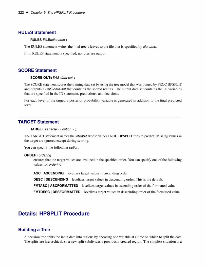
322 F Chapter 9: The HPSPLIT Procedure
RULES StatementRULES FILE=filename ;
The RULES statement writes the final tree’s leaves to the file that is specified by filename.
If no RULES statement is specified, no rules are output.
SCORE StatementSCORE OUT=SAS-data-set ;
The SCORE statement scores the training data set by using the tree model that was trained by PROC HPSPLITand outputs a SAS-data-set that contains the scored results. The output data set contains the ID variablesthat are specified in the ID statement, predictions, and decisions.
For each level of the target, a posterior probability variable is generated in addition to the final predictedlevel.
TARGET StatementTARGET variable < / option > ;
The TARGET statement names the variable whose values PROC HPSPLIT tries to predict. Missing values inthe target are ignored except during scoring.
You can specify the following option:
ORDER=orderingensures that the target values are levelized in the specified order. You can specify one of the followingvalues for ordering:
ASC | ASCENDING levelizes target values in ascending order.
DESC | DESCENDING levelizes target values in descending order. This is the default.
FMTASC | ASCFORMATTED levelizes target values in ascending order of the formatted value.
FMTDESC | DESFORMATTED levelizes target values in descending order of the formatted value.
Details: HPSPLIT Procedure
Building a TreeA decision tree splits the input data into regions by choosing one variable at a time on which to split the data.The splits are hierarchical, so a new split subdivides a previously created region. The simplest situation is a
Interval Input Binning Details F 323
binary split, where only two regions are created from an input region. An interval variable is split by whetherthe region is less than or is greater than or equal to the split value. Nominal values are collected into twogroups.
These hierarchical splits form a tree: the splits are represented by the tree nodes, and the resulting regions arerepresented by the leaves. Figure 9.3 shows an illustration of a tree and how the space is partitioned by it.The left diagram shows the tree (subdivided region letters are shaded). The splits occur at the tree nodes, andthe leaves are the final regions of the input space. The right diagram shows how the input space is partitionedby the tree. The original data set is the region A, which does not appear on the right. Region A is split intoregions B and C by the interval variable X. Region C is subdivided again, this time by the variable Y, intoregions D and E. Because the largest number of splits that occur in a path from the top of the tree to thebottommost region is two, the depth of this example tree is two.
Figure 9.3 Conceptual Drawing of a Decision Tree
Tree Partitioned Input Space
Interval Input Binning DetailsPROC HPSPLIT places interval input variables into bins. You can specify the number of bins by using theINTERVALBINS= option in the PROC HPSPLIT statement. Each bin except the last spans the range�
vmax � vmin
intervalbinsbinC vmin;
vmax � vmin
intervalbins.binC 1/C vmin
�where vmax and vmin are the maximum and minimum value of the respective variable and bin is the bin,which is an integer in the range
Œ0; intervalbins/
For the largest bin, the end of the bin range is inclusive.

324 F Chapter 9: The HPSPLIT Procedure
Input Variable Splitting and SelectionYou can use the following criteria to determine a split:
• entropy
• FastCHAID
• Gini
PROC HPSPLIT determines the best split in two stages. First, the splitter uses a splitting algorithm categoryto find the best split for each variable according to the criterion. Next, the variable that has the best splitdetermines the split of the leaf.
The splitter uses different algorithms called splitting categories to find the best split for a variable. Threecategories are available: exhaustive, a C4.5-like greedy algorithm that groups levels together using thecriterion that is specified in the CRITERION statement until the value specified in the MAXBRANCH=option is reached, and a fast sort–based greedy algorithm. The splitter switches between the differentalgorithms as the number of levels increases because each splitting category has a different computationalcomplexity that depends on the number of levels.
Splitting Categories and Types
The number of available levels in the variable to be split determines the splitting category. A variable’s levelis “available” if the variable has not yet been used in the path from the root of the tree to the leaf that isbeing split, or if a given level has not been switched to a different branch along that path. This definition of“available” allows a variable to be split multiple times. Adjusting the splitting category based on the numberof available levels obtains the best split possible according to the statistical criterion while still enabling thesplitter to perform quickly despite dealing with an arbitrary number of variable levels or bins.
An exhaustive split search of an interval variable has a much different computational complexity than anexhaustive split search of a nominal variable does. Because of this difference, only two splitter categories areused for interval variables: the exhaustive search and a fast, greedy search. The exhaustive search examinesevery possible arrangement of splits, up to one less than the value specified in the MAXBRANCH option.The best one is chosen as that variable’s split.
If an exhaustive search is computationally infeasible—that is, it requires more operations to perform thanthe value specified in the LEVTHRESH2= option—the splitter falls back to a faster, greedy algorithm. Thegreedy algorithm finds the best single split. It then finds the best split of the resulting two regions, choosingthe best region and the best split of that region. This process continues until the number of regions equals thevalue specified in the MAXBRANCH= option or until no further splits are possible.
An exhaustive search of nominal variable splits requires checking every possible assignment of levels toresulting regions. Therefore, the number of operations that are required to perform this search is exponentialas a function of the number of variable levels. If the number of operations that are required to perform theexhaustive search is greater than the value specified in the LEVTHRESH1= option, then the splitter uses afaster, greedy search.
The fast greedy algorithm examines each possible pairwise combination of levels. The splitter looks at thebest pairwise combination of levels and merges the best pair. This process continues until the number of
Pruning F 325
splits is below one less than the value specified in the MAXBRANCH= option. However, if the number oflevels is huge, even this method is infeasible, and the splitter falls back to an even faster method.
After ordering the nominal variable levels based on the EVENT= option, the splitter finds the best splitsiteratively. At each iteration, the best split is chosen using the statistical metric for each previously split rangeof bins or levels. In effect, this combines a number of binary-split nodes into one ensemble of one less thanthe number of splits specified in the MAXBRANCH= option.
For FastCHAID, the splitter uses only the fastest algorithm regardless of the number of levels. The statistic thatis used for choosing split goodness is the Kolmogorov-Smirnov (K-S) distance for the empirical cumulativedistribution function. The K-S splitter follows Friedman’s (1977) proposal, splitting once at the point thathas the maximum K-S distance between all the levels. The splitter then finds the maximum K-S distance ofthe resulting regions and splits there. The splitter continues until the number of splits is equal to the valuespecified in the MAXBRANCH= option minus 1.
Selecting the Split Variable
After it finds the split for each variable, the splitter uses the criterion from the CRITERION statement tochoose the best split variable to use for the final tree node. The entropy and Gini criteria use the namedmetric to guide the decision.
FastCHAID uses the p-value of the two-way table of target-child counts of the proposed split. The ALPHA=option in the PROC HPSPLIT statement (default of 0.3) is the value below which the p-value must fall inorder to be accepted as a candidate split. In addition, the BONFERRONI keyword in the PROC HPSPLITstatement causes the p-value of the split (which was determined by Kolmogorov-Smirnov distance) to beadjusted using the Bonferroni adjustment.
The splitting metrics are based on the population that lands at the node, not the whole tree. For example, thechange in entropy when you split the leaf into a node is determined by the number of observations at thatleaf. Although subtle, this distinction makes it potentially useful to grow and prune according to the entropy,even when no validation data set is present. This is because the metric that is used in pruning is based on thepartition of the entire data set.
PruningYou can choose to prune by the following pattern, which uses the by-metric to choose a node to prune back toa leaf at each iteration until the per-leaf change in the until-metric is operator value times the per-leaf changein the until-metric of replacing the full tree with a single leaf:
PRUNE by-metric / until-metric operator value;
For example, the following statement prunes by average square error until the number of leaves falls below(or is equal to) 3:
PRUNE ASE / N <= 3;
The inequality is necessary because PROC HPSPLIT prunes by removing entire nodes and replacing themwith leaves.
326 F Chapter 9: The HPSPLIT Procedure
The by-metric is used to choose the node to prune back to a leaf. The smallest global increase (or largestdecrease) in the specified metric is the criterion used to choose the node to prune. After the pruner choosesthe leaf, it uses the until-metric to determine whether to terminate pruning.
For example, consider the following statement.
PRUNE GINI / ENTROPY >= 1.0;
This statement chooses the node with the lowest global change (smallest increase or largest decrease) in theGini statistic when the node is made into a leaf, and it terminates when removing the node causes a changein global entropy per leaf that is greater than or equal to the per-leaf change in entropy that is caused byreplacing the original tree by a single leaf.
To be more precise, if the original tree had an entropy E0 and N0 leaves and trimming away the whole tree toa stump had an entropy of Es (and, because it is a stump, just one leaf), the per-leaf change in entropy is
�E
�N
ˇ0
DE0 �Es
N0 � 1
If the node, n, that is chosen by the pruner has an entropy En and Nn leaves and has an entropy of E� if itwere replaced by leaf, then
�E
�N
ˇn
DEn �E�
Nn � 1
The preceding statement would cause the pruner to terminate when
�E�N
ˇn
�E�N
ˇ0
� 1
For all until-metrics except N, the default operator is >= and the default value is 1.0. For the N until-metric,the default operator is <= and the default value is 5.
Memory ConsiderationsPROC HPSPLIT is built for high-performance computing. As a result, it does not create utility files butrather stores all the data in memory. Data sets that have a large number of variables and few observations,particularly if they have a large number of target levels, can cause PROC HPSPLIT to run out of memory.One way to overcome this is to give SAS more memory to use. Another way to deal with this is to use fewerthreads.
Handling Missing ValuesWhen building and pruning a tree, PROC HPSPLIT ignores observations that have a missing value in thetarget. It includes these observations when using the SCORE statement to score the data, and it includes themin the SAS DATA step code.

Handling Unknown Levels in Scoring F 327
PROC HPSPLIT always includes observations that have missing values in input variables. It uses a speciallevel or bin for them that is not used in per-variable split determination. After the splitter has determined theper-variable split, the observations that have a missing value in that variable are assigned to the leaf that hasthe largest number of observations.
Each split handles missing values by assigning them to one of the children. This ensures that data scored bythe SAS DATA step score code can always assign a target to any record.
Handling Unknown Levels in ScoringPROC HPSPLIT treats nominal variable values that do not occur in the input data set (either in the validationor in the training set) as missing values in the generated SAS DATA step scoring code.
PROC HPSPLIT assigns interval variables that are outside the minimum and maximum range in the inputdata (the training and validation sets together) to either of the end bins. PROC HPSPLIT assigns a value lessthan the minimum to the first bin and a value greater than the maximum to the last bin.
Splitting CriteriaWhen you specify entropy or the Gini statistic as the splitting criterion, the value of the split is judged by thedecrease in the specified criterion. Thus, the criterion for the original leaf is computed, as is the criterion forthe final, split leaf. The per-variable split and then the variable on which to split are chosen based on the gain.
When you specify FastCHAID as the splitting criterion, splitting is based on the Kolmogorov-Smirnovdistance of the variables.
Entropy Splitting Criterion
The entropy is related to the amount of information that a split contains. The entropy of a single leaf � isgiven by the equation
Entropy� D �Xt
N �t
N�log2
N �t
N�
!
whereN �t is the number of observations with the target level t on leaf � andN� is the number of observations
on the leaf (Hastie, Tibshirani, and Friedman 2001; Quinlan 1993).
When a leaf is split, the total entropy is then
Entropy D �X�
N�
N0
Xt
N �t
N�log2
N �t
N�
!
where N0 is the number of observations on the original unsplit leaf.

328 F Chapter 9: The HPSPLIT Procedure
Gini Splitting Criterion
Split Gini is similar to split entropy. First, the per-leaf Gini statistic or index is given by Hastie, Tibshirani,and Friedman (2001) as
Gini� DXt
N �t
N�
1 �
N �t
N�
!
When split, the Gini statistic is then
Gini DX N�
N0
Xt
N �t
N�
1 �
N �t
N�
!
Kolmogorov-Smirnov (FastCHAID) Splitting Criterion
The Kolmogorov-Smirnov (K-S) distance is the maximum distance between the cumulative distributionfunctions (CDFs) of two or more target levels (Friedman 1977; Rokach and Maimon 2008; Utgoff and Clouse1996). To create a meaningful CDF for nominal inputs, nominal target levels are ordered first by the levelthat is specified in the EVENT= option in the PROC HPSPLIT statement (if specified) and then by the otherlevels in internal order.
After the CDFs have been created, the maximum K-S distance is given by
MAXKS D MAXijkˇCDF
�ji � CDF
�ki
ˇwhere i is an interval variable bin or an explanatory variable level, �j is the jth target level, and �k is the kthtarget level.
At each step of determining each variable’s split, the maximum K-S distance is computed, resulting in asingle split. The splitting continues recursively until the value specified in the MAXBRANCH= option hasbeen reached.
After each variable’s split has been determined, the variable that has the lowest p-value is chosen as thevariable on which to split. Because this operation is similar to another established tree algorithm (Kass 1980;Soman, Diwakar, and Ajay 2010), this overall criterion is called “FastCHAID.”
Pruning CriteriaPruning criteria are similar to growth criteria, except that they use the global change of a metric instead ofthe per-leaf change. In addition, if a validation partition is present, pruning statistics are calculated from that.
Entropy Pruning Criterion
When you prune by entropy, the entropy is calculated as though the entire data set were a single leafpartitioned into the final number of leaves. Thus it can be expected that the pruning path taken during pruningmight not correspond to the reverse of the path taken during growth, even if the pruning and growth metricsare identical.
The change is then based on the global entropy with the node preserved and the node pruned back to a leaf.

Subtree Statistics F 329
Gini Pruning Criterion
As with entropy, the change in Gini statistic is calculated based on the change in the global Gini statistic. Theequations are otherwise unchanged.
Misclassification Rate Pruning Criterion
The misclassification rate (MISC) is simply the number of mispredictions divided by the number of predictions.Thus, for a leaf that has a predicted target level, �P , the misclassification rate is
MISC� DX�i¤�P
N ��i
N�
For all the leaves in the tree, it is
MISC DX�
N�
N0
X�i¤�P
N ��i
N�
The predicted target level is always based on the training data set.
Average Square Error Pruning Criterion
The average square error (ASE) is based on the sum of squares error (SSE). You would expect, for a perfectassignment, that the proportion of observations at a leaf � would be 1 for the predicted target level and 0 forthe remainder. Thus, for a single leaf, the equation for the average of this error is
ASE� D 1 � 2X�i
Nƒ�i
Nƒ
N ��i
N�C
X�i
N ��i
N�
!2where � is for a leaf in the training set and ƒ is for a leaf in the validation set. If there is no validation set, thetraining set is used.
Thus, for an ensemble of leaves the ASE becomes
ASE DXƒ
N�
N0
241 � 2X�i
Nƒ�i
Nƒ
N ��i
N�C
X�i
N ��i
N�
!235This summation is over the validation counts set at the leaves, ƒ.
Subtree StatisticsStatistics that are printed in the subtree tables are similar to the pruning statistics. There are two ways tocalculate the subtree statistics: one is based on a scored data set (using the SCORE statement or the SASDATA step score code that the CODE statement produces), and the other is based on the internal observationcounts at each leaf of the tree. The two methods should provide identical results unless the target is missing.
NOTE: The per-observation and per-leaf methods of calculating the subtree statistics might not agree if theinput data set contains observations that have a missing value for the target.
330 F Chapter 9: The HPSPLIT Procedure
Per-Observation Methods
In scoring, whether you use the SCORE statement or you use the CODE statement with a SAS DATA step,each observation is assigned a posterior probability, P� , where � is a target level. These posterior probabilitiesare then used to calculate the subtree statistics of the final tree.
For a leaf �, the posterior probability is the fraction of observations at that leaf that have the target level � .That is, for that leaf �
P �� DN ��
N�
When a record is scored, it is assigned to a leaf, and all posterior probabilities for that leaf are assigned alongwith it. Thus, for observation ! assigned to leaf �, the posterior probability is
P !� D P�� D
N ��
N�
The variable N0 continues to indicate the total number of observations in the input data set, and ! is theobservation number (! is used to prevent confusion with 0).
If a validation set is selected, the per-observation statistics are calculated separately for each. In addition, theper-observation validation posterior probabilities should be used. The validation posterior probabilities, V !� ,are the same as the posterior probabilities from the training set, but they are the fraction of observations fromthe validation set that are in each target level,
V !� D V�� D
N ��
N�
where N �� and N� are now observation counts from the validation set. For calculating the statistics on the
validation set, the same equations can be used but substituting V for P where appropriate (for example, V ��for P �� ).
Observationwise Entropy StatisticThe entropy at each observation is calculated from the posterior probabilities:
Entropy D �X!
1
N0
X�
P !� log2�P !�
�
Observationwise Gini StatisticLike the entropy, the Gini statistic is also calculated from the posterior probabilities:
Gini DX!
1
N0
X�
P !��1 � P !�
�
Subtree Statistics F 331
Observationwise Misclassification RateThe misclassification rate is the average number of incorrectly predicted observations in the input data set.Predictions are always based on the training set. Thus, each scored record’s predicted target level �!P iscompared against the actual level �!� :
MISC DX!
1 � ı�!P �!�
N0
ı�!P �!�
is the Kronecker delta:
ı�!P �!�D
�1 if �!p D �
!�
0 otherwise
Or, phrased slightly differently, the misclassification rate is the fraction of incorrectly predicted observations:
MISC D1
N0
X!
�0 if �!p D �
!�
1 otherwise
Observationwise Sum of Squares ErrorFor the sum of squares error (SSE), N� predictions are made for every observation: that the correct posterioris 1 and that the incorrect posteriors is 0. Thus the SSE is as follows, with �!� once again being the actualtarget level for observation !:
SSE DX!
24 X�¤�!�
�P !�
�2C
�1 � P !�!�
�235
Observationwise Average Square ErrorThe average square error (ASE) is simply the SSE divided by the number of predictions (there are N�predictions per observation):
ASE D1
N�N0
X!
24 X�¤�!�
�P !�
�2C�1 � P�!�
�235
Per-Leaf Methods
The subtree statistics that are calculated by PROC HPSPLIT are calculated per leaf. That is, instead ofscanning through the entire data set, the proportions of observations are examined at the leaves. Barringmissing target values, which are not handled by the tree, the per-leaf and per-observation methods forcalculating the subtree statistics are the same.
As with the per-observation method, observation counts N (N �� , N�, and N0) can come from either the
training set or the validation set. The growth subtree table always produces statistics from the training set.The pruning subtree table produces both sets of data if they are both present.
Unless otherwise marked, counts N can come from either set.
332 F Chapter 9: The HPSPLIT Procedure
Leafwise Entropy StatisticBecause there are N� observations on the leaf �, entropy takes the following form:
Entropy D �X�
N�
N0
X�
P �� log2�P ��
�Rephrased in terms of N, this becomes
Entropy D �X�
N�
N0
X�
N ��
N�log2
N ��
N�
!
Leafwise Gini StatisticThe Gini statistic is similar to entropy in its leafwise form:
Gini DX�
N�
N0
X�
P ��
�1 � P ��
�Rephrased in terms of N, this becomes
Gini DX�
N�
N0
X�
N ��
N�
1 �
N ��
N�
!
Leafwise Misclassification RateMisclassification comes from the number of incorrectly predicted observations. Thus, it is necessary to countthe proportion of observations at each leaf in each target level. The misprediction rate of a single leaf, similarto the misprediction rate of an entire data set, is
MISC� D1
N�
X!
�0 if �!p D �
!�
1 otherwise
where the summation is over the observations that arrive at a leaf �.
All observations at a leaf are assigned the same prediction because they are all assigned the same leaf.Therefore, the summation reduces to simply the number of observations at leaf � that have a target level otherthan the predicted target level for that leaf, �� . Thus,
MISC� DN� �N
���
N�
D
X�¤��
N ��
N�
D
X�¤��
P ��
where P �� is V �� if the validation set is being examined.
Subtree Statistics F 333
Thus, for the entire data set, the misclassification rate is
MISC DX N�
N0
X�¤��
P ��
D
X N�
N0
X�¤��
N ��
N�
where again P �� is V �� for the validation set.
Leafwise Sum of Squares ErrorThe sum of squares error (SSE) is treated similarly to the misclassification rate. Each observation is assignedper-target posterior probabilities P �� from the training data set. These are the predictions for the purpose ofthe SSE.
The observations at leaf � are then grouped by the observations’ target levels. Because each observation inthe group has the same actual target level, ˆ, and because all observations on the same node are assigned thesame posterior probabilities, P �� , the per-observation SSE equation is identical:
SSE�ˆ DX!2ˆ
24 X�¤�ˆ�
�P ��
�2C
�1 � P �
�ˆ�
�235D N �
ˆ
24 X�¤�ˆ�
�P ��
�2C
�1 � P �
�ˆ�
�235Here, the posterior probabilities P �� are from the training set, and the counts themselves N �
� are fromwhichever data set is being examined.
Thus, the SSE equation for the leaf can be rephrased in terms of a further summation over the target levels ˆ:
SSE� DXˆ
N �ˆ
24 X�¤�ˆ�
�P ��
�2C
�1 � P �
�ˆ�
�235So the SSE for the entire tree is then
SSE DX�
Xˆ
N �ˆ
24 X�¤�ˆ�
�P ��
�2C
�1 � P �
�ˆ�
�235

334 F Chapter 9: The HPSPLIT Procedure
Substituting the counts from the training set back in and using � to denote training set counts, this becomes
SSE DX�
Xˆ
N �ˆ
264 X�¤�ˆ�
�����
!2C
0@1 � ���ˆ���
1A2375
D
X�
Xˆ
N �ˆ
264 X�¤�ˆ�
�����
!2C 1 � 2
���ˆ�
��C
0@���ˆ���
1A2375
D
X�
Xˆ
N �ˆ
24X�
�����
!2C 1 � 2
���ˆ�
��C
35D
X�
N�Xˆ
N �ˆ
N�
24X�
�����
!2C 1 � 2
���ˆ�
��
35D
X�
N�
241CX�
�����
!2� 2
Xˆ
N �ˆ
N�
���ˆ�
��
35Now, in that rightmost inner summation, �ˆ� is simply ˆ, the target level being summed over. This gives thefinal equivalent forms
SSE DX�
N�
241CX�
�����
!2� 2
Xˆ
N �ˆ
N�
��ˆ��
35SSE D
X�
N�
"1C
X�
�P ��
�2� 2
Xˆ
V �ˆP�ˆ
#
where � and P are again counts and fraction, respectively, from the training set, and N and V are counts andfraction, respectively, from the validation set. (For example, N �
ˆ is the number of observations on leaf � withtarget ˆ.)
If there is no validation set, the training set is used instead, and the equations simplify to the following(because ˆ is merely an index over target levels and can be renamed � ):
SSE DX�
N�
241 �X�
�����
!235SSE D
X�
N�
"1 �
X�
�P ��
�2#
Variable Importance F 335
Leafwise Average Square ErrorBecause average square error (ASE) is simply the SSE divided by the number of predictions (there are N� ,the number of target levels, predictions per observation), this becomes
ASE DX�
N�
N�N0
241CX�
�����
!2� 2
Xˆ
N �ˆ
N�
��ˆ��
35ASE D
X�
N�
N�N0
"1C
X�
�P ��
�2� 2
Xˆ
V �ˆP�ˆ
#
Or, if only the training set is used:
SSE DX�
N�
N�N0
241 �X�
�����
!235SSE D
X�
N�
N�N0
"1 �
X�
�P ��
�2#
Variable ImportanceVariable importance is calculated based on how the variables are used in the finished tree. Three metrics areused: count, SSE, and relative importance. The count-based variable importance simply counts the number oftimes in the entire tree that a given variable is used in a split. The SSE and relative importance are calculatedfrom the training set. They are also calculated again from the validation set if one exists. These are reportedas “VSSE” and “VIMPORT.”
The SSE-based variable importance is based on the nodes in which the variable is used in a split. For eachvariable, the change of the SSE that results from the split is found. The change is
�� D SSE� �X�
SSE��
where � denotes the node. SSE� is then the SSE if the node is treated as a leaf, and SSE��
is the SSE of thenode after it has been split. If the change in SSE is negative (which is possible when you use the validationset), then the change is set to 0.
The SSE-based importance is then
SSEIMPORTvariable D
vuutvariable nodesX�
��
The relative importance metric is based on the SSE of each variable. The maximum SSE variable importanceis found. Then all the variables are assigned a relative importance, which is simply
IMPORTvariable DSSEIMPORTvariable
SSEIMPORTmax

336 F Chapter 9: The HPSPLIT Procedure
Outputs
Performance Information
The “Performance Information” table is created by default. It displays information about the execution mode.For single-machine mode, the table displays the number of threads used. For distributed mode, the tabledisplays the grid mode (symmetric or asymmetric), the number of compute nodes, and the number of threadsper node.
Output Data Sets
SCORE Data SetTable 9.3 shows the variables that are contained in an example data set that the SCORE statement produces.In this data set, the variable BAD is the target and has values 0 and 1.
Table 9.3 Example SCORE Statement Data Set Variables
Variable Description
BAD Target variable_LEAF_ Leaf number to which this observation is assigned_NODE_ Node number to which this observation is assignedP_BAD0 Proportion of training set at this leaf that has BAD = 0P_BAD1 Proportion of training set at this leaf that has BAD = 1V_BAD0 Proportion of validation set at this leaf that has BAD = 0V_BAD1 Proportion of validation set at this leaf that has BAD = 1
IMPORTANCE= Data SetThe variable importance data set contains the importance of the input variables in creating the pruned decisiontree. A simple count-based importance metric and two variable importance metrics that are based on the sumof squares error-based are output. In addition, the number of observations that are used in the training andvalidation sets, the number of observations that have a missing value, and the number of observations thathave a missing target are output. Table 9.4 shows the variables contained in the data set that the OUTPUTstatement produces using the IMPORTANCE= option. In addition to the variables listed below, a variablecontaining the importance for each input variable is included.
Table 9.4 Variable Importance Data Set Variables
Variable Description
TREENUM Tree number (always 1)CRITERION Criterion used to generate the treeITYPE Importance type (“Count”, “SSE”, “VSSE”, “IMPORT”, or “VIMPORT”)OBSMISS Number of observations that have a missing valueOBSTMISS Number of observations that have a missing targetOBSUSED Number of observations used to build the tree (training set)OBSVALID Number of observations in the validation set

Outputs F 337
NODESTATS= Data SetThe data set specified in the NODESTATS= option in the OUTPUT statement can be used to visualize thetree. Table 9.5 shows the variables in this data set.
Table 9.5 NODESTATS= Data Set Variables
Variable Description
ALLTEXT Text that describes the splitCRITERION Which of the three criteria was usedDECISION Values of the parent variable’s split to get to this nodeDEPTH Depth of the nodeID Node numberLINKWIDTH Fraction of all training observations going to this nodeN Number of training observations at this nodeNVALID Number of validation observations at this nodePARENT Parent’s node numberPREDICTEDVALUE Value of target predicted at this nodeP_BAD0 Proportion of training observations that have BAD=0P_BAD1 Proportion of training observations that have BAD=1SPLITVAR Variable used in the splitTREENUM Tree number (always 1)V_BAD0 Proportion of validation observations that have BAD=0V_BAD1 Proportion of validation observations that have BAD=1
GROWTHSUBTREE= and PRUNESUBTREE= Data SetsDuring tree growth and pruning, the number of leaves at each growth or pruning iteration is output in additionto other, optional metrics.
The GROWTHSUBTREE= and PRUNESUBTREE= data sets are identical, except that:
• The growth data set reflects statistics of the tree during growth. The pruning data set reflects statisticsof the tree during pruning.
• The statistics of the growth data set are always from the training subset. The statistics of the pruningdata set are from the validation subset if one is available. Otherwise, the statistics of the pruning dataset are from the training subset.
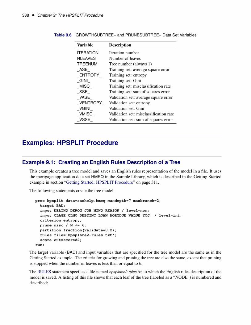
338 F Chapter 9: The HPSPLIT Procedure
Table 9.6 GROWTHSUBTREE= and PRUNESUBTREE= Data Set Variables
Variable Description
ITERATION Iteration numberNLEAVES Number of leavesTREENUM Tree number (always 1)_ASE_ Training set: average square error_ENTROPY_ Training set: entropy_GINI_ Training set: Gini_MISC_ Training set: misclassification rate_SSE_ Training set: sum of squares error_VASE_ Validation set: average square error_VENTROPY_ Validation set: entropy_VGINI_ Validation set: Gini_VMISC_ Validation set: misclassification rate_VSSE_ Validation set: sum of squares error
Examples: HPSPLIT Procedure
Example 9.1: Creating an English Rules Description of a TreeThis example creates a tree model and saves an English rules representation of the model in a file. It usesthe mortgage application data set HMEQ in the Sample Library, which is described in the Getting Startedexample in section “Getting Started: HPSPLIT Procedure” on page 311.
The following statements create the tree model.
proc hpsplit data=sashelp.hmeq maxdepth=7 maxbranch=2;target BAD;input DELINQ DEROG JOB NINQ REASON / level=nom;input CLAGE CLNO DEBTINC LOAN MORTDUE VALUE YOJ / level=int;criterion entropy;prune misc / N <= 6;partition fraction(validate=0.2);rules file='hpsplhme2-rules.txt';score out=scored2;
run;
The target variable (BAD) and input variables that are specified for the tree model are the same as in theGetting Started example. The criteria for growing and pruning the tree are also the same, except that pruningis stopped when the number of leaves is less than or equal to 6.
The RULES statement specifies a file named hpsplhme2-rules.txt, to which the English rules description of themodel is saved. A listing of this file shows that each leaf of the tree (labeled as a “NODE”) is numbered anddescribed:
Example 9.1: Creating an English Rules Description of a Tree F 339
*------------------------------------------------------------*NODE = 2
*------------------------------------------------------------*DELINQ IS ONE OF 5, 6, 7, 8, 10, 11, 12, 13, 15AND DELINQ IS ONE OF 1, 2, 3, 4, 5, 6, 7, 8, 10, 11, 12, 13, 15
PREDICTED VALUE IS 1PREDICTED 1 = 0.9342( 71/76)PREDICTED 0 = 0.06579( 5/76)
*------------------------------------------------------------*NODE = 4
*------------------------------------------------------------*NINQ IS ONE OF 4, 5, 6, 8, 9, 10, 11, 12, 13, 14, 17AND DELINQ IS ONE OF MISSING, 1, 2, 3, 4AND DELINQ IS ONE OF 1, 2, 3, 4, 5, 6, 7, 8, 10, 11, 12, 13, 15
PREDICTED VALUE IS 1PREDICTED 1 = 0.8714( 61/70)PREDICTED 0 = 0.1286( 9/70)
*------------------------------------------------------------*NODE = 5
*------------------------------------------------------------*NINQ IS ONE OF MISSING, 0, 1, 2, 3, 7AND DELINQ IS ONE OF MISSING, 1, 2, 3, 4AND DELINQ IS ONE OF 1, 2, 3, 4, 5, 6, 7, 8, 10, 11, 12, 13, 15
PREDICTED VALUE IS 0PREDICTED 1 = 0.3682( 306/831)PREDICTED 0 = 0.6318( 525/831)
*------------------------------------------------------------*NODE = 8
*------------------------------------------------------------*DEBTINC IS MISSING OR DEBTINC <45.137782AND CLAGE IS MISSING OR CLAGE <186.91737AND DELINQ IS ONE OF MISSING, 0
PREDICTED VALUE IS 0PREDICTED 1 = 0.1739( 392/2254)PREDICTED 0 = 0.8261( 1862/2254)
*------------------------------------------------------------*NODE = 9
*------------------------------------------------------------*DEBTINC >=45.137782AND CLAGE IS MISSING OR CLAGE <186.91737AND DELINQ IS ONE OF MISSING, 0
PREDICTED VALUE IS 1PREDICTED 1 = 1( 37/37)PREDICTED 0 = 0( 0/37)
*------------------------------------------------------------*NODE = 10
*------------------------------------------------------------*CLAGE >=186.91737AND DELINQ IS ONE OF MISSING, 0
PREDICTED VALUE IS 0PREDICTED 1 = 0.0589( 90/1528)PREDICTED 0 = 0.9411( 1438/1528)

340 F Chapter 9: The HPSPLIT Procedure
The listing includes each leaf of the tree, along with the proportion of training set observations that arein the region that is represented by the respective leaf. The predicted value is shown for each leaf, alongwith the fraction of that leaf’s observations that is in each of the target levels. The nodes are not numberedconsecutively in the order 1, 2, 3, and so on, because the non-leaf nodes are not included.
The splits that lead to each leaf are shown above the predicted value and fractions. The same variable can beinvolved in more than one split. For instance, the leaf labeled “NODE = 2” covers the region where DELINQis between 1 and 8, between 10 and 13, or is equal to 15, and the region where DELINQ is also between 5 and8, between 10 and 13, or is equal to 15. In other words, the variable DELINQ is split twice in succession.
By preserving multiple splits of the same variable rather than merging them, the rules description makes itpossible to traverse the splits from the bottom of the tree to the top. For the leaf labeled “NODE=10”, the dataset was first split on DELINQ and the subset with DELINQ=0 or where the value for DELINQ was missingwere split again on CLAGE, with those observations having CLAGE >=186.91737 going to node 10. At thisleaf (node 10), the predicted value for BAD is 0 because the majority of the observations (94%) have value 0.
The SCORE statement saves scores for the observations in a SAS data set named SCORED2. Output 9.1.1lists the first ten observations of SCORED2.
Output 9.1.1 Scored Input Data Set (HMEQ)
Obs BAD _NODE_ _LEAF_ P_BAD1 P_BAD0 V_BAD1 V_BAD0
1 1 8 3 0.17391 0.82609 0.18808 0.811922 1 5 2 0.36823 0.63177 0.36126 0.638743 1 8 3 0.17391 0.82609 0.18808 0.811924 1 8 3 0.17391 0.82609 0.18808 0.811925 0 8 3 0.17391 0.82609 0.18808 0.811926 1 8 3 0.17391 0.82609 0.18808 0.811927 1 5 2 0.36823 0.63177 0.36126 0.638748 1 8 3 0.17391 0.82609 0.18808 0.811929 1 5 2 0.36823 0.63177 0.36126 0.63874
10 1 8 3 0.17391 0.82609 0.18808 0.81192
The variables _LEAF_ and _NODE_ show the leaf to which the observation was assigned. The variablesP_BAD0 and P_BAD1 are the proportions of observations in the training set that have BAD=1 and BAD=0for that leaf. The variables V_BAD0 and V_BAD1 are the proportions of observations in the validation setthat have BAD=1 and BAD=0 for that leaf. For information about the variables in the scored data set, see thesection “Outputs” on page 336.
Example 9.2: Assessing Variable ImportanceDuring the manufacture of a semiconductor device, the levels of temperature, atomic composition, and otherparameters are vital to ensuring that the final device is usable. This example creates a decision tree model forthe performance of finished devices.
The following statements create a data set named MBE_DATA, which contains measurements for 20 devices:
Example 9.2: Assessing Variable Importance F 341
data mbe_data;label gtemp = 'Growth Temperature of Substrate';label atemp = 'Anneal Temperature';label rot = 'Rotation Speed';label dopant = 'Dopant Atom';label usable = 'Experiment Could be Performed';
input gtemp atemp rot dopant $ 35-37 usable $ 43-51;datalines;384.614 633.172 1.01933 C Unusable363.874 512.942 0.72057 C Unusable397.395 671.179 0.90419 C Unusable389.962 653.940 1.01417 C Unusable387.763 612.545 1.00417 C Unusable394.206 617.021 1.07188 Si Usable387.135 616.035 0.94740 Si Usable428.783 745.345 0.99087 Si Unusable399.365 600.932 1.23307 Si Unusable455.502 648.821 1.01703 Si Unusable387.362 697.589 1.01623 Ge Usable408.872 640.406 0.94543 Ge Usable407.734 628.196 1.05137 Ge Usable417.343 612.328 1.03960 Ge Usable482.539 669.392 0.84249 Ge Unusable367.116 564.246 0.99642 Sn Unusable398.594 733.839 1.08744 Sn Unusable378.032 619.561 1.06137 Sn Usable357.544 606.871 0.85205 Sn Unusable384.578 635.858 1.12215 Sn Unusable;run;
The variables GTEMP and ATEMP are temperatures, ROT is a rotation speed, and DOPANT is the atom thatis used during device growth. The variable USABLE indicates whether the device is usable.
The following statements create the tree model:
proc hpsplit data=mbe_data maxdepth=1;target usable;input gtemp atemp rot dopant;output importance=import;prune none;
run;
There is only one INPUT statement because all of the numeric variables are interval inputs.
The MAXDEPTH=1 option specifies that the tree is to stop splitting when the maximum specified depthof one is reached. In other words, PROC HPSPLIT tries to split the data by each input variable and thenchooses the best variable on which to split the data. The split that is chosen divides the data into higher andlower incidences of the target variable (USABLE). The PRUNE statement suppresses pruning because thereis only one split.
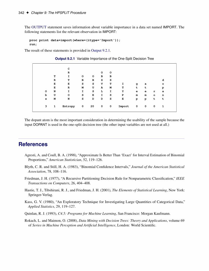
342 F Chapter 9: The HPSPLIT Procedure
The OUTPUT statement saves information about variable importance in a data set named IMPORT. Thefollowing statements list the relevant observation in IMPORT:
proc print data=import(where=(itype='Import'));run;
The result of these statements is provided in Output 9.2.1.
Output 9.2.1 Variable Importance of the One-Split Decision Tree
CR O O
T I O O B BR T B B S S dE E S S V T I g a oE R M U A M T t t p
O N I I S L I Y e e r ab U O S E I S P m m o ns M N S D D S E p p t t
3 1 Entropy 0 20 0 0 Import 0 0 0 1
The dopant atom is the most important consideration in determining the usability of the sample because theinput DOPANT is used in the one-split decision tree (the other input variables are not used at all.)
References
Agresti, A. and Coull, B. A. (1998), “Approximate Is Better Than ‘Exact’ for Interval Estimation of BinomialProportions,” American Statistician, 52, 119–126.
Blyth, C. R. and Still, H. A. (1983), “Binomial Confidence Intervals,” Journal of the American StatisticalAssociation, 78, 108–116.
Friedman, J. H. (1977), “A Recursive Partitioning Decision Rule for Nonparametric Classification,” IEEETransactions on Computers, 26, 404–408.
Hastie, T. J., Tibshirani, R. J., and Friedman, J. H. (2001), The Elements of Statistical Learning, New York:Springer-Verlag.
Kass, G. V. (1980), “An Exploratory Technique for Investigating Large Quantities of Categorical Data,”Applied Statistics, 29, 119–127.
Quinlan, R. J. (1993), C4.5: Programs for Machine Learning, San Francisco: Morgan Kaufmann.
Rokach, L. and Maimon, O. (2008), Data Mining with Decision Trees: Theory and Applications, volume 69of Series in Machine Perception and Artificial Intelligence, London: World Scientific.

References F 343
Soman, K. P., Diwakar, S., and Ajay, V. (2010), Insight into Data Mining: Theory and Practice, New Delhi:PHI Learning.
Utgoff, P. E. and Clouse, J. A. (1996), A Kolmogorov-Smirnov Metric for Decision Tree Induction, TechnicalReport 96-3, University of Massachusetts, Amherst.
Wilson, E. B. (1927), “Probable Inference, the Law of Succession, and Statistical Inference,” Journal of theAmerican Statistical Association, 22, 209–212.

344
Subject Index
2D geometric anisotropic structureHPLMIXED procedure, 203
adaptive lasso selectionhigh-performance statistical procedures,
SELECTION statement, 68Akaike’s information criterion
MIXED procedure, 220Akaike’s information criterion (finite sample corrected
version)MIXED procedure, 220
alpha levelHPGENSELECT procedure, 89HPLMIXED procedure, 199, 202HPLOGISTIC procedure, 146
ANCOVA effectsShared Concepts, 56
ANOVA effectsShared Concepts, 56
ANOVA tableHPREG procedure, 291
ANTE(1) structureHPLMIXED procedure, 203
antedependence structureHPLMIXED procedure, 203
AR(1) structureHPLMIXED procedure, 203
association statisticsHPLOGISTIC procedure, 165
at sign (@) operatorShared Concepts, 54, 57
autoregressive moving-average structureHPLMIXED procedure, 203
autoregressive structureHPLMIXED procedure, 203
backward eliminationhigh-performance statistical procedures,
SELECTION statement, 63banded Toeplitz structure
HPLMIXED procedure, 203bar (|) operator
Shared Concepts, 54, 56, 57bar (|) operator
Shared Concepts, 56Bernoulli distribution
HPNLMOD procedure, 238binary distribution
HPNLMOD procedure, 238
binomial distributionHPNLMOD procedure, 238
BLUEHPLMIXED procedure, 216
BLUPHPLMIXED procedure, 216
boundary constraints, 237HPLMIXED procedure, 200, 201
boundsHPNLMOD procedure, 237
candidates for addition or removalHPGENSELECT procedure, 112HPREG procedure, 290
class levelHPGENSELECT procedure, 83, 111HPLMIXED procedure, 197HPLOGISTIC procedure, 140, 162HPREG procedure, 274, 289MIXED procedure, 218
CLASS statementShared Concepts, 50
classification variablesShared Concepts, 50
colon (:) operatorShared Concepts, 55
complete separationHPLOGISTIC procedure, 155
compound symmetry structureexample (HPLMIXED), 210HPLMIXED procedure, 203
computational methodHPGENSELECT procedure, 106HPLMIXED procedure, 217HPLOGISTIC procedure, 157HPNLMOD procedure, 248HPREG procedure, 287
confidence limitsmodel parameters (HPGENSELECT), 89model parameters (HPLOGISTIC), 146
constraintsboundary (HPLMIXED), 200, 201
continuous-by-class effectsShared Concepts, 59
continuous-nesting-class effectsShared Concepts, 58
convergence criterionHPGENSELECT procedure, 80–82
346 F Subject Index
HPLMIXED procedure, 194, 195HPLOGISTIC procedure, 137–139HPNLMOD procedure, 233, 234MIXED procedure, 219
convergence statusHPGENSELECT procedure, 113HPLOGISTIC procedure, 163MIXED procedure, 220
correlation matrixHPGENSELECT procedure, 81, 114
covariance matrixHPGENSELECT procedure, 81, 114
covariance parameter estimatesMIXED procedure, 220
covariance structureantedependence (HPLMIXED), 206autoregressive (HPLMIXED), 206autoregressive moving average (HPLMIXED),
206banded (HPLMIXED), 207compound symmetry (HPLMIXED), 206equi-correlation (HPLMIXED), 206examples (HPLMIXED), 204factor-analytic (HPLMIXED), 206heterogeneous autoregressive (HPLMIXED), 206heterogeneous compound symmetry
(HPLMIXED), 206heterogeneous Toeplitz (HPLMIXED), 207HPLMIXED procedure, 188, 203Huynh-Feldt (HPLMIXED), 207simple (HPLMIXED), 207Toeplitz (HPLMIXED), 207unstructured (HPLMIXED), 207unstructured, correlation (HPLMIXED), 207variance components (HPLMIXED), 207
crossed effectsShared Concepts, 57
dash (-) operatorShared Concepts, 55
degrees of freedomHPLMIXED procedure, 199infinite (HPLMIXED), 199method (HPLMIXED), 199residual method (HPLMIXED), 199
diagnostic statisticsHPREG procedure, 283
dimension informationMIXED procedure, 218
dimensionsHPGENSELECT procedure, 114HPLOGISTIC procedure, 164HPREG procedure, 289
direct product structure
HPLMIXED procedure, 203displayed output
HPGENSELECT procedure, 111HPLMIXED procedure, 218HPLOGISTIC procedure, 161HPNLMOD procedure, 252HPREG procedure, 289
distributed computingHPLMIXED procedure, 217
distribution functionHPGENSELECT procedure, 89
distribution functionsHPNLMOD procedure, 246
double dash (- -) operatorShared Concepts, 55
effectname length (HPGENSELECT), 83name length (HPLMIXED), 197name length (HPLOGISTIC), 140name length (HPREG), 274
empirical Bayes estimateHPNLMOD procedure, 242
estimationmixed model (HPLMIXED), 214
estimation methodsHPLMIXED procedure, 196
examples, HPLMIXEDcompound symmetry, G-side setup, 211compound symmetry, R-side setup, 211holding covariance parameters fixed, 200specifying lower bounds, 200split-plot design, 212subject and no-subject formulation, 211unstructured covariance, G-side, 203
examples, HPNLMOD procedureboundary specification, 237conditional model expression, 257enzyme data, 229gamma distribution, 247join point, 257plateau model, 257predicted values, 257segmented model, 257starting values, data set, 241starting values, grid, 240
factor analytic structuresHPLMIXED procedure, 203
fit criteriaHPREG procedure, 282
fit statisticsHPGENSELECT procedure, 114HPLOGISTIC procedure, 164
Subject Index F 347
HPREG procedure, 291fixed effects
HPLMIXED procedure, 188fixed-effects parameters
HPLMIXED procedure, 210forward selection
high-performance statistical procedures,SELECTION statement, 61
forward swap selectionhigh-performance statistical procedures,
SELECTION statement, 66frequency variable
high-performance statistical procedures, 44HPGENSELECT procedure, 85HPLOGISTIC procedure, 143HPREG procedure, 276
G matrixHPLMIXED procedure, 188, 201, 210
gamma distributionHPNLMOD procedure, 238
Gaussian distributionHPNLMOD procedure, 238
general distributionHPNLMOD procedure, 238
general effectsShared Concepts, 59
general linear covariance structureHPLMIXED procedure, 203
generalized inverse, 216global tests
HPLOGISTIC procedure, 164gradient
MIXED procedure, 219growth curve analysis
example (HPLMIXED), 210
Hessian matrixHPLMIXED procedure, 219
heterogeneousAR(1) structure (HPLMIXED), 203compound-symmetry structure (HPLMIXED),
203covariance structure (HPLMIXED), 207Toeplitz structure (HPLMIXED), 203
high-performance statistical procedures, SELECTIONstatement
adaptive lasso selection, 68backward elimination, 63forward selection, 61forward swap selection, 66LAR selection, 67LASSO selection, 67stepwise selection, 64
Hosmer-Lemeshow testHPLOGISTIC procedure, 147, 156, 157, 164
HPGENSELECT procedure, 71alpha level, 89candidates for addition or removal, 112class level, 83, 111computational method, 106confidence limits, 89convergence criterion, 80–82convergence status, 113correlation matrix, 81, 114covariance matrix, 81, 114dimensions, 114displayed output, 111distribution function, 89effect name length, 83fit statistics, 114function-based convergence criteria, 80, 81gradient-based convergence criteria, 81, 82input data sets, 81iteration history, 113link function, 90model information, 111model options summary, 86multithreading, 94, 106number of observations, 111ODS table names, 115optimization technique, 107parameter estimates, 114performance information, 111response level ordering, 87response profile, 112response variable options, 87selected effects, 113selection details, 112selection information, 112selection reason, 113selection summary, 112stop reason, 113user-defined formats, 82weighting, 95XML input stream, 82zero inflation link function, 96zero-inflation parameter estimates, 115
HPLMIXED procedure, 1862D geometric anisotropic structure, 203alpha level, 199, 202ANTE(1) structure, 203antedependence structure, 203AR(1) structure, 203ARMA structure, 203autoregressive moving-average structure, 203autoregressive structure, 203banded Toeplitz structure, 203
348 F Subject Index
BLUE, 195, 216BLUP, 195, 216boundary constraints, 200, 201chi-square test, 199class level, 197compound symmetry structure, 203, 210computational method, 217confidence interval, 202confidence limits, 199, 202convergence criterion, 194, 195covariance structure, 188, 203, 204degrees of freedom, 199direct product structure, 203displayed output, 218distributed computing, 217EBLUPs, 202, 217effect name length, 197estimation methods, 196factor analytic structures, 203fixed effects, 188fixed-effects parameters, 199, 210function-based convergence criteria, 194, 195G matrix, 188, 201, 210general linear covariance structure, 203generalized inverse, 216gradient-based convergence criteria, 194, 195grid search, 199growth curve analysis, 210Hessian matrix, 219heterogeneous AR(1) structure, 203heterogeneous compound-symmetry structure,
203heterogeneous covariance structures, 207heterogeneous Toeplitz structure, 203Huynh-Feldt structure, 203infinite degrees of freedom, 199infinite likelihood, 208initial values, 199input data sets, 195intercept effect, 199, 202Kronecker product structure, 203linear covariance structure, 203Matérn covariance structure, 203matrix notation, 209mixed model, 210mixed model equations, 215mixed model theory, 209multi-threading, 201multithreading, 217Newton-Raphson algorithm, 215ODS table names, 221optimization information, 219parameter constraints, 200parameter-based convergence criteria, 197
performance information, 218R matrix, 188, 208, 210random effects, 188, 201random-effects parameters, 202, 210repeated measures, 208residual method, 199restricted maximum likelihood (REML), 187ridging, 215spatial anisotropic exponential structure, 203split-plot design, 212standard linear model, 188statement positions, 192subject effect, 202, 208summary of commands, 193table names, 221timing, 221Toeplitz structure, 203unstructured correlations, 203unstructured covariance matrix, 203variance components, 203variance ratios, 200
HPLOGISTIC procedure, 127alpha level, 146association statistics, 165class level, 140, 162complete separation, 155computational method, 157confidence limits, 146convergence criterion, 137–139convergence status, 163dimensions, 164displayed output, 161effect name length, 140existence of MLEs, 154fit statistics, 164function-based convergence criteria, 137, 138global tests, 164gradient-based convergence criteria, 138, 139Hosmer-Lemeshow test, 147, 156, 157, 164infinite parameter estimates, 154input data sets, 138iteration history, 163link function, 147model information, 162model options summary, 144multithreading, 150, 157number of observations, 162ODS table names, 165optimization technique, 158parameter estimates, 165performance information, 161quasi-complete separation, 155response level ordering, 144response profile, 162
Subject Index F 349
response variable options, 144selected effects, 163selection information, 162selection reason, 163selection summary, 162separation, 154stop reason, 163user-defined formats, 138weighting, 151XML input stream, 138
HPNLMOD procedure, 227additional estimates, 237, 254additional estimates correlation, 255additional estimates covariance, 255ANOVA, 254Bernoulli distribution, 238binary distribution, 238binomial distribution, 238bounds, 237computational method, 248convergence criterion, 233, 234convergence status, 253correlation, 255covariance, 254dimensions, 253displayed output, 252distribution functions, 246empirical Bayes estimate, 242fit statistics, 254function-based convergence criteria, 233, 234gamma distribution, 238Gaussian distribution, 238general distribution, 238gradient-based convergence criteria, 233, 234initial values, 239input data sets, 233iteration history, 253lag functionality, 244least squares, 245least squares distribution, 238linear constraints, 253log-likelihood functions, 246multithreading, 241, 248negative binomial distribution, 238normal distribution, 238number of observations, 253ODS table names, 255optimization technique, 249output data sets, 236parameter estimates, 254parameters, 253performance information, 252Poisson distribution, 238prediction, 242
procedure task timing, 255programming statements, 243residual distribution, 238restrictions, 243segmented model example, 256specifications, 252starting values, 239user-defined formats, 234, 236XML input stream, 234, 236
HPREG procedure, 263ANOVA table, 291candidates for addition or removal, 290class level, 274, 289computational method, 287diagnostic statistics, 283dimensions, 289displayed output, 289effect name length, 274fit criteria, 282fit statistics, 291input data sets, 273introductory example, 266model information, 289multithreading, 278, 287number of observations, 289ODS table names, 293output data set, 288parameter estimates, 292performance information, 289random number seed, 274selected effects, 291selection information, 289selection reason, 290selection summary, 290stop reason, 290test data, 286timing, 292user-defined formats, 273validation, 286weighting, 281XML input stream, 273
Huynh-Feldtstructure (HPLMIXED), 203
infinite likelihoodHPLMIXED procedure, 208
infinite parameter estimatesHPLOGISTIC procedure, 154
initial valuesHPLMIXED procedure, 199HPNLMOD procedure, 239
interaction effectsShared Concepts, 57
intercept
350 F Subject Index
Shared Concepts, 56iteration history
HPGENSELECT procedure, 113HPLOGISTIC procedure, 163MIXED procedure, 219
iterationshistory (MIXED), 219
Kronecker product structureHPLMIXED procedure, 203
lag functionalityHPNLMOD procedure, 244
LAR selectionhigh-performance statistical procedures,
SELECTION statement, 67LASSO selection
high-performance statistical procedures,SELECTION statement, 67
least squaresHPNLMOD procedure, 245
least squares distributionHPNLMOD procedure, 238
levelizationShared Concepts, 50
linear covariance structureHPLMIXED procedure, 203
link functionHPGENSELECT procedure, 90HPLOGISTIC procedure, 147
log-likelihood functionsHPNLMOD procedure, 246
main effectsShared Concepts, 56
Matérn covariance structureHPLMIXED procedure, 203
matrixnotation, theory (HPLMIXED), 209
maximum likelihoodestimates (HPLOGISTIC), 154
maximum likelihood estimationmixed model (HPLMIXED), 215
mixed model (HPLMIXED)estimation, 214formulation, 210maximum likelihood estimation, 215notation, 188theory, 209
mixed model (MIXED)objective function, 219
mixed model equationsHPLMIXED procedure, 215
MIXED procedureAkaike’s information criterion, 220
Akaike’s information criterion (finite samplecorrected version), 220
class level, 218convergence criterion, 219convergence status, 220covariance parameter estimates, 220dimension information, 218fitting information, 220gradient, 219iteration history, 219iterations, 219model information, 218number of observations, 218Schwarz’s Bayesian information criterion, 220
modelinformation (HPGENSELECT), 111information (HPLOGISTIC), 162information (HPREG), 289specification (HPNLMOD procedure, 238
model informationMIXED procedure, 218
multi-threadingHPLMIXED procedure, 201
multithreadingHPGENSELECT procedure, 94, 106HPLMIXED procedure, 217HPLOGISTIC procedure, 150, 157HPNLMOD procedure, 241, 248HPREG procedure, 278, 287
negative binomial distributionHPNLMOD procedure, 238
nested effectsShared Concepts, 58
nested versus crossed effectsShared Concepts, 58
Newton-Raphson algorithmHPLMIXED procedure, 215
normal distributionHPNLMOD procedure, 238
number of observationsHPGENSELECT procedure, 111HPLOGISTIC procedure, 162HPREG procedure, 289MIXED procedure, 218
objective functionmixed model (MIXED), 219
optimization informationHPLMIXED procedure, 219
optimization techniqueHPGENSELECT procedure, 107HPLOGISTIC procedure, 158HPNLMOD procedure, 249
Subject Index F 351
options summaryMODEL statement (HPLMIXED), 198PROC HPGENSELECT statement, 79PROC HPLMIXED statement, 193PROC HPLOGISTIC statement, 136PROC HPNLMOD statement, 232PROC HPREG statement, 273RANDOM statement (HPLMIXED), 202REPEATED statement (HPLMIXED), 208
orderingof class levels (Shared Concepts), 51
output data setHPREG procedure, 288
overlap of data pointsHPLOGISTIC procedure, 155
parameter constraintsHPLMIXED procedure, 200
parameter estimatesHPGENSELECT procedure, 114HPLOGISTIC procedure, 165HPREG procedure, 292
parameterizationShared Concepts, 52
performance informationHPGENSELECT procedure, 111HPLMIXED procedure, 218HPLOGISTIC procedure, 161HPREG procedure, 289
Poisson distributionHPNLMOD procedure, 238
polynomial effectsShared Concepts, 56
predictionHPNLMOD procedure, 242
programming statementsHPNLMOD procedure, 243
quasi-complete separationHPLOGISTIC procedure, 155
R matrixHPLMIXED procedure, 188, 208, 210
random effectsHPLMIXED procedure, 188, 201
random-effects parametersHPLMIXED procedure, 210
regression effectsShared Concepts, 56
repeated measuresHPLMIXED procedure, 208
residual distributionHPNLMOD procedure, 238
residual maximum likelihood (REML)HPLMIXED procedure, 215
response level orderingHPGENSELECT procedure, 87HPLOGISTIC procedure, 144
response profileHPGENSELECT procedure, 112HPLOGISTIC procedure, 162
response variable optionsHPGENSELECT procedure, 87HPLOGISTIC procedure, 144
restricted maximum likelihoodHPLMIXED procedure, 187
restricted maximum likelihood (REML)HPLMIXED procedure, 215
restrictionsHPNLMOD procedure, 243
reverse response level orderingHPGENSELECT procedure, 87HPLOGISTIC procedure, 144
ridgingHPLMIXED procedure, 215
Schwarz’s Bayesian information criterionMIXED procedure, 220
selected effectsHPGENSELECT procedure, 113HPLOGISTIC procedure, 163HPREG procedure, 291
selection detailsHPGENSELECT procedure, 112
selection informationHPGENSELECT procedure, 112HPLOGISTIC procedure, 162HPREG procedure, 289
selection reasonHPGENSELECT procedure, 113HPLOGISTIC procedure, 163HPREG procedure, 290
selection summaryHPGENSELECT procedure, 112HPLOGISTIC procedure, 162HPREG procedure, 290
separationHPLOGISTIC procedure, 154
Shared ConceptsANCOVA effects, 56ANOVA effects, 56at sign (@) operator, 54, 57bar (|) operator, 54, 56, 57bar (|) operator, 56CLASS statement, 50classification variables, 50colon (:) operator, 55continuous-by-class effects, 59continuous-nesting-class effects, 58
352 F Subject Index
crossed effects, 57dash (-) operator, 55double dash (- -) operator, 55general effects, 59interaction effects, 57intercept, 56levelization, 50main effects, 56missing values, class variables, 52nested effects, 58nested versus crossed effects, 58ORDER= option, 51ordering of class levels, 51parameterization, 52polynomial effects, 56regression effects, 56singular parameterization, 57sort order of class levels, 51
singular parameterizationShared Concepts, 57
sort orderof class levels (Shared Concepts), 51
spatial anisotropic exponential structureHPLMIXED procedure, 203
split-plot designHPLMIXED procedure, 212
standard linear modelHPLMIXED procedure, 188
starting valuesHPNLMOD procedure, 239
stepwise selectionhigh-performance statistical procedures,
SELECTION statement, 64stop reason
HPGENSELECT procedure, 113HPLOGISTIC procedure, 163HPREG procedure, 290
subject effectHPLMIXED procedure, 202, 208
summary of commandsHPLMIXED procedure, 193
table namesHPLMIXED procedure, 221
test dataHPREG procedure, 286
timingHPLMIXED procedure, 221HPREG procedure, 292
Toeplitz structureHPLMIXED procedure, 203
unstructured correlationsHPLMIXED procedure, 203
unstructured covariance matrixHPLMIXED procedure, 203
validationHPREG procedure, 286
variance componentsHPLMIXED procedure, 203
variance ratiosHPLMIXED procedure, 200
weightingHPGENSELECT procedure, 95HPLOGISTIC procedure, 151HPREG procedure, 281
zero inflation link functionHPGENSELECT procedure, 96
zero-inflation parameter estimatesHPGENSELECT procedure, 115

Syntax Index
ABSCONV optionPROC HPGENSELECT statement, 80PROC HPLMIXED statement, 194PROC HPLOGISTIC statement, 137PROC HPNLMOD statement, 233
ABSFCONV optionPROC HPGENSELECT statement, 80PROC HPLMIXED statement, 194PROC HPLOGISTIC statement, 137PROC HPNLMOD statement, 233
ABSGCONV optionPROC HPGENSELECT statement, 81PROC HPLMIXED statement, 194PROC HPLOGISTIC statement, 138PROC HPNLMOD statement, 233
ABSGTOL optionPROC HPGENSELECT statement, 81PROC HPLMIXED statement, 194PROC HPLOGISTIC statement, 138PROC HPNLMOD statement, 233
ABSOLUTE optionPROC HPLMIXED statement, 219
ABSTOL optionPROC HPGENSELECT statement, 80PROC HPLMIXED statement, 194PROC HPLOGISTIC statement, 137PROC HPNLMOD statement, 233
ADAPTIVE optionSELECTION statement (high-performance
statistical procedures), 46ALPHA= option
ESTIMATE statement (HPNLMOD), 238MODEL statement (HPGENSELECT), 89MODEL statement (HPLOGISTIC), 146OUTPUT statement (HPGENSELECT), 93PREDICT statement (HPNLMOD), 242PROC HPGENSELECT statement, 81PROC HPLOGISTIC statement, 138PROC HPNLMOD statement, 233PROC HPREG statement, 273RANDOM statement (HPLMIXED), 202
ASSOCIATION optionMODEL statement (HPLOGISTIC), 146
BLUP optionPROC HPLMIXED statement, 195
BOUNDS statementHPNLMOD procedure, 237
BY statementHPLOGISTIC procedure, 141HPNLMOD procedure, 237HPREG procedure, 274
CHOOSE= optionMODEL statement (high-performance statistical
procedures), 46CL option
MODEL statement (HPGENSELECT), 89MODEL statement (HPLMIXED), 199MODEL statement (HPLOGISTIC), 146RANDOM statement (HPLMIXED), 202
CLASS statementhigh-performance statistical procedures, 40HPGENSELECT procedure, 84HPLMIXED procedure, 198HPLOGISTIC procedure, 142HPREG procedure, 275MIXED procedure, 218
CLB optionMODEL statement (HPREG), 276
CODE statementHPGENSELECT procedure, 85HPGENSELECT procedure, 85HPLOGISTIC procedure, 142HPREG procedure, 275
COMMIT= optionPERFORMANCE statement (high-performance
analytical procedures), 34COMPETITIVE option
SELECTION statement (high-performancestatistical procedures), 46
CONVF optionPROC HPLMIXED statement, 219
CONVG optionPROC HPLMIXED statement, 219
CONVH optionPROC HPLMIXED statement, 219
COPYVAR= optionOUTPUT statement (HPLOGISTIC), 149OUTPUT statement (HPREG), 280
CORR optionPROC HPGENSELECT statement, 81PROC HPNLMOD statement, 233
COV optionPROC HPGENSELECT statement, 81PROC HPNLMOD statement, 233

354 F Syntax Index
CRITERION statementHPSPLIT procedure, 316
CRITERION= optionSELECTION statement (high-performance
statistical procedures), 46
DATA= optionOUTPUT statement (HPGENSELECT), 92OUTPUT statement (HPLOGISTIC), 149OUTPUT statement (HPREG), 280PROC HPGENSELECT statement, 81PROC HPLMIXED statement, 195PROC HPLOGISTIC statement, 138PROC HPNLMOD statement, 233PROC HPREG statement, 273
DATASERVER= optionPERFORMANCE statement (high-performance
analytical procedures), 34DDFM= option
MODEL statement (HPLMIXED), 199MODEL statement (HPLOGISTIC), 146
DESCENDING optionCLASS statement (high-performance statistical
procedures), 40MODEL statement (HPGENSELECT), 87MODEL statement (HPLOGISTIC), 144
DETAILS optionPERFORMANCE statement (high-performance
analytical procedures), 35DETAILS= option
SELECTION statement (high-performancestatistical procedures), 48
DF= optionESTIMATE statement (HPNLMOD), 238PREDICT statement (HPNLMOD), 242PROC HPNLMOD statement, 234
DISPERSION= optionMODEL statement (HPGENSELECT), 89
DISTRIBUTION= optionMODEL statement (HPGENSELECT), 89
ECORR optionPROC HPNLMOD statement, 234
ECOV optionPROC HPNLMOD statement, 234
EQCONS= optionPARMS statement (HPLMIXED), 200
ESTIMATE statementHPNLMOD procedure, 238
FAST optionSELECTION statement (high-performance
statistical procedures), 47FCONV option
PROC HPGENSELECT statement, 81
PROC HPLMIXED statement, 195PROC HPLOGISTIC statement, 138PROC HPNLMOD statement, 234
FMTLIBXML= optionPROC HPGENSELECT statement, 82PROC HPLOGISTIC statement, 138PROC HPNLMOD statement, 234PROC HPREG statement, 273
FRACTION optionHPREG procedure, PARTITION statement, 278HPSPLIT procedure, PARTITION statement, 319
FREQ statementhigh-performance statistical procedures, 44HPGENSELECT procedure, 85HPLOGISTIC procedure, 143HPREG procedure, 276
FTOL optionPROC HPGENSELECT statement, 81PROC HPLMIXED statement, 195PROC HPLOGISTIC statement, 138PROC HPNLMOD statement, 234
GCONV optionPROC HPGENSELECT statement, 82PROC HPLMIXED statement, 195PROC HPLOGISTIC statement, 139PROC HPNLMOD statement, 234
GRIDHOST= optionPERFORMANCE statement (high-performance
analytical procedures), 35GRIDMODE= option
PERFORMANCE statement (high-performanceanalytical procedures), 35
GRIDTIMEOUT= optionPERFORMANCE statement (high-performance
analytical procedures), 35GTOL option
PROC HPGENSELECT statement, 82PROC HPLMIXED statement, 195PROC HPLOGISTIC statement, 139PROC HPNLMOD statement, 234
HIERARCHY= optionSELECTION statement (high-performance
statistical procedures), 49high-performance analytical procedures,
PERFORMANCE statement, 34COMMIT= option, 34DATASERVER= option, 34DETAILS option, 35GRIDHOST= option, 35GRIDMODE= option, 35GRIDTIMEOUT= option, 35HOST= option, 35

Syntax Index F 355
INSTALL= option, 35INSTALLLOC= option, 35LASR= option, 35LASRSERVER= option, 35MODE= option, 35NNODES= option, 36NODES= option, 36NTHREADS= option, 37THREADS= option, 37TIMEOUT= option, 35
high-performance statistical proceduresFREQ statement, 44ID statement, 44VAR statement, 50WEIGHT statement, 50
high-performance statistical procedures, CLASSstatement, 40
DESCENDING option, 40MISSING option, 43ORDER= option, 41PARAM= option, 43REF= option, 41TRUNCATE= option, 44
high-performance statistical procedures, FREQstatement, 44
high-performance statistical procedures, ID statement,44
high-performance statistical procedures, SELECTIONstatement, 45
ADAPTIVE option, 46CHOOSE= option, 46COMPETITIVE option, 46CRITERION= option, 46DETAILS= option, 48HIERARCHY= option, 49LSCOEFFS option, 47MAXEFFECTS= option, 47MAXSTEP= option, 47METHOD= option, 45MINEFFECTS= option, 47SELECT= option, 47SELECTION= option, 49SLE= option, 47SLENTRY= option, 47SLS= option, 48SLSTAY= option, 48STOP= option, 48STOPHORIZON= option, 49
high-performance statistical procedures, VARstatement, 50
high-performance statistical procedures, WEIGHTstatement, 50
HOLD= optionPARMS statement (HPLMIXED), 200
HOST= optionPERFORMANCE statement (high-performance
analytical procedures), 35HPGENSELECT procedure, 79
CLASS statement, 84CODE statement, 85FREQ statement, 85ID statement, 86MODEL statement, 86OUTPUT statement, 92PERFORMANCE statement, 94PROC HPGENSELECT statement, 79SELECTION statement, 94syntax, 79WEIGHT statement, 95ZEROMODEL statement, 96
HPGENSELECT procedure, CLASS statement, 84UPCASE option, 85
HPGENSELECT procedure, CODE statement, 85HPGENSELECT procedure, FREQ statement, 85HPGENSELECT procedure, ID statement, 86HPGENSELECT procedure, MODEL statement, 86
ALPHA= option, 89CL option, 89DESCENDING option, 87DISPERSION= option, 89DISTRIBUTION= option, 89INCLUDE option, 90INITIALPHI= option, 90LINK= option, 90NOCENTER option, 91NOINT option, 91OFFSET= option, 91ORDER= option, 88SAMPLEFRAC= option, 91START option, 91
HPGENSELECT procedure, OUTPUT statement, 92ALPHA= option, 93DATA= option, 92keyword= option, 92OBSCAT option, 94OUT= option, 92
HPGENSELECT procedure, PERFORMANCEstatement, 94
HPGENSELECT procedure, PROC HPGENSELECTstatement, 79
ABSCONV option, 80ABSFCONV option, 80ABSFTOL option, 80ABSGCONV option, 81ABSGTOL option, 81ABSTOL option, 80ALPHA= option, 81CORR option, 81

356 F Syntax Index
COV option, 81DATA= option, 81FCONV option, 81FMTLIBXML= option, 82FTOL option, 81GCONV option, 82GTOL option, 82ITDETAILS option, 82ITSELECT option, 82MAXFUNC= option, 82MAXITER= option, 83MAXTIME= option, 83NAMELEN= option, 83NOCLPRINT option, 83NOPRINT option, 83NORMALIZE= option, 83NOSTDERR option, 83SINGCHOL= option, 84SINGSWEEP= option, 84SINGULAR= option, 84TECHNIQUE= option, 84
HPGENSELECT procedure, SELECTION statement,94
HPGENSELECT procedure, WEIGHT statement, 95HPGENSELECT procedure, ZEROMODEL statement,
96INCLUDE option, 96START option, 96
HPGENSELECT procedure, CODE statement, 85HPLMIXED procedure, 192
PERFORMANCE statement, 201PROC HPLMIXED statement, 193syntax, 192
HPLMIXED procedure, CLASS statement, 198HPLMIXED procedure, MODEL statement, 198
CL option, 199DDFM= option, 199NOINT option, 199SOLUTION option, 199
HPLMIXED procedure, PARMS statement, 199EQCONS= option, 200HOLD= option, 200LOWERB= option, 200NOITER option, 201PARMSDATA= option, 201PDATA= option, 201UPPERB= option, 201
HPLMIXED procedure, PERFORMANCE statement,201
HPLMIXED procedure, PROC HPLMIXED statementABSCONV option, 194ABSFCONV option, 194ABSFTOL option, 194ABSGCONV option, 194
ABSGTOL option, 194ABSTOL option, 194BLUP option, 195DATA= option, 195FCONV option, 195FTOL option, 195GCONV option, 195GTOL option, 195MAXCLPRINT= option, 196MAXFUNC= option, 196MAXITER= option, 196MAXTIME= option, 196METHOD= option, 196NAMELEN= option, 197NOCLPRINT option, 197NOPRINT option, 197SINGCHOL= option, 197SINGSWEEP= option, 197SINGULAR= option, 197TECHNIQUE= option, 197XCONV option, 197XTOL option, 197
HPLMIXED procedure, RANDOM statement, 201ALPHA= option, 202CL option, 202SOLUTION option, 202SUBJECT= option, 202TYPE= option, 203
HPLMIXED procedure, REPEATED statement, 208SUBJECT= option, 208TYPE= option, 208
HPLMIXEDC procedure, PROC HPLMIXEDstatement, 193
HPLOGISTIC procedure, 136CLASS statement, 142FREQ statement, 143ID statement, 143MODEL statement, 143OUTPUT statement, 148PERFORMANCE statement, 150PROC HPLOGISTIC statement, 136SELECTION statement, 150syntax, 136WEIGHT statement, 151
HPLOGISTIC procedure, BY statement, 141HPLOGISTIC procedure, CLASS statement, 142
UPCASE option, 143HPLOGISTIC procedure, FREQ statement, 143HPLOGISTIC procedure, ID statement, 143HPLOGISTIC procedure, MODEL statement, 143
ALPHA= option, 146ASSOCIATION option, 146CL option, 146DDFM= option, 146

Syntax Index F 357
DESCENDING option, 144INCLUDE option, 147LACKFIT option, 147LINK= option, 147NOCHECK option, 148NOINT option, 148OFFSET= option, 148ORDER= option, 145RSQUARE option, 148START option, 148
HPLOGISTIC procedure, OUTPUT statement, 148COPYVAR= option, 149DATA= option, 149keyword= option, 149OBSCAT option, 150OUT= option, 149
HPLOGISTIC procedure, PERFORMANCEstatement, 150
HPLOGISTIC procedure, PROC HPLOGISTICstatement, 136
ABSCONV option, 137ABSFCONV option, 137ABSFTOL option, 137ABSGCONV option, 138ABSGTOL option, 138ABSTOL option, 137ALPHA= option, 138DATA= option, 138FCONV option, 138FMTLIBXML= option, 138FTOL option, 138GCONV option, 139GTOL option, 139ITDETAILS option, 139ITSELECT option, 139MAXFUNC= option, 139MAXITER= option, 139, 140MAXTIME= option, 140NAMELEN= option, 140NOCLPRINT option, 140NOITPRINT option, 140NOPRINT option, 140NORMALIZE= option, 140NOSTDERR option, 140SINGCHOL= option, 141SINGSWEEP= option, 141SINGULAR= option, 141TECHNIQUE= option, 141
HPLOGISTIC procedure, SELECTION statement, 150HPLOGISTIC procedure, WEIGHT statement, 151HPLOGISTIC procedure, CODE statement, 142HPNLMOD procedure, 231
PERFORMANCE statement, 241PROC HPNLMOD statement, 232
syntax, 231HPNLMOD procedure, BOUNDS statement, 237HPNLMOD procedure, BY statement, 237HPNLMOD procedure, ESTIMATE statement, 238
ALPHA= option, 238DF= option, 238
HPNLMOD procedure, MODEL statement, 238HPNLMOD procedure, PARAMETERS statement,
239HPNLMOD procedure, PERFORMANCE statement,
241HPNLMOD procedure, PREDICT statement, 242
ALPHA= option, 242DF= option, 242LOWER= option, 242PRED= option, 242PROBT= option, 242STDERR= option, 242TVALUE= option, 242UPPER= option, 242
HPNLMOD procedure, PROC HPNLMOD statement,232
ABSCONV option, 233ABSFCONV option, 233ABSFTOL option, 233ABSGCONV option, 233ABSGTOL option, 233ABSTOL option, 233ALPHA= option, 233CORR option, 233COV option, 233DATA= option, 233DF= option, 234ECORR option, 234ECOV option, 234FCONV option, 234FMTLIBXML= option, 234FTOL option, 234GCONV option, 234GTOL option, 234MAXFUNC= option, 235MAXITER= option, 235MAXTIME= option, 235NOITPRINT option, 236NOPRINT option, 236OUT= option, 236SINGULAR= option, 236TECHNIQUE= option, 236XMLFORMAT= option, 236
HPNLMOD procedure, RESTRICT statement, 243HPREG procedure
FREQ statement, 276ID statement, 276MODEL statement, 276
358 F Syntax Index
OUTPUT statement, 279PARTITION statement, 278PERFORMANCE statement, 278PROC HPREG statement, 273WEIGHT statement, 281
HPREG procedure, BY statement, 274HPREG procedure, CLASS statement, 275
SPLIT option, 42UPCASE option, 275
HPREG procedure, ID statement, 276HPREG procedure, MODEL statement, 276
CLB option, 276INCLUDE option, 277NOINT option, 277ORDERSELECT option, 277START option, 277STB option, 277TOL option, 277VIF option, 277
HPREG procedure, OUTPUT statement, 279COPYVAR= option, 280DATA= option, 280keyword= option, 280OUT= option, 280
HPREG procedure, PARTITION statement, 278FRACTION option, 278ROLEVAR= option, 278
HPREG procedure, PERFORMANCE statement, 278HPREG procedure, PROC HPREG statement, 273
ALPHA= option, 273DATA= option, 273FMTLIBXML= option, 273NAMELEN= option, 274NOCLPRINT option, 274NOPRINT option, 274SEED= option, 274
HPREG procedure, SELECTION statement, 278HPREG procedure, WEIGHT statement, 281HPREG procedures, FREQ statement, 276HPREG procedure, CODE statement, 275HPSPLIT procedure
CRITERION statement, 316ID statement, 317INPUT statement, 317OUTPUT statement, 318PARTITION statement, 319PERFORMANCE statement, 320PROC HPSPLIT statement, 314PRUNE statement, 320RULES statement, 316, 322SCORE statement, 322TARGET statement, 322
HPSPLIT procedure, CRITERION statement, 316HPSPLIT procedure, ID statement, 317
HPSPLIT procedure, INPUT statement, 317HPSPLIT procedure, OUTPUT statement, 318HPSPLIT procedure, PARTITION statement, 319
FRACTION option, 319ROLEVAR= option, 319
HPSPLIT procedure, PERFORMANCE statement, 320HPSPLIT procedure, PROC HPSPLIT statement, 314HPSPLIT procedure, PRUNE statement, 320HPSPLIT procedure, RULES statement, 316, 322HPSPLIT procedure, SCORE statement, 322HPSPLIT procedure, TARGET statement, 322
ID statementhigh-performance statistical procedures, 44HPGENSELECT procedure, 86HPLOGISTIC procedure, 143HPREG procedure, 276HPSPLIT procedure, 317
INCLUDE optionMODEL statement (HPGENSELECT), 90MODEL statement (HPLOGISTIC), 147MODEL statement (HPREG), 277ZEROMODEL statement (HPGENSELECT), 96
INITIALPHI= optionMODEL statement (HPGENSELECT), 90
INPUT statementHPSPLIT procedure, 317
INSTALL= optionPERFORMANCE statement (high-performance
analytical procedures), 35INSTALLLOC= option
PERFORMANCE statement (high-performanceanalytical procedures), 35
ITDETAILS optionPROC HPGENSELECT statement, 82PROC HPLOGISTIC statement, 139
ITSELECT optionPROC HPGENSELECT statement, 82PROC HPLOGISTIC statement, 139
keyword= optionOUTPUT statement (HPGENSELECT), 92OUTPUT statement (HPLOGISTIC), 149OUTPUT statement (HPREG), 280
LACKFIT optionMODEL statement (HPLOGISTIC), 147
LASR= optionPERFORMANCE statement (high-performance
analytical procedures), 35LASRSERVER= option
PERFORMANCE statement (high-performanceanalytical procedures), 35
LINK= optionMODEL statement (HPGENSELECT), 90

Syntax Index F 359
MODEL statement (HPLOGISTIC), 147LOWER= option
PREDICT statement (HPNLMOD), 242LOWERB= option
PARMS statement (HPLMIXED), 200LSCOEFFS option
SELECTION statement (high-performancestatistical procedures), 47
MAXCLPRINT= optionPROC HPLMIXED statement, 196
MAXEFFECTS= optionSELECTION statement (high-performance
statistical procedures), 47MAXFUNC= option
PROC HPGENSELECT statement, 82PROC HPLMIXED statement, 196PROC HPLOGISTIC statement, 139PROC HPNLMOD statement, 235
MAXITER= optionPROC HPGENSELECT statement, 83PROC HPLMIXED statement, 196PROC HPLOGISTIC statement, 139, 140PROC HPNLMOD statement, 235
MAXSTEPS= optionSELECTION statement (high-performance
statistical procedures), 47MAXTIME= option
PROC HPGENSELECT statement, 83PROC HPLMIXED statement, 196PROC HPLOGISTIC statement, 140PROC HPNLMOD statement, 235
METHOD= optionPROC HPLMIXED statement, 196SELECTION statement (high-performance
statistical procedures), 45MINEFFECTS= option
SELECTION statement (high-performancestatistical procedures), 47
MISSING optionCLASS statement (high-performance statistical
procedures), 43MIXED procedure, CLASS statement, 218MIXED procedure, PROC HPLMIXED statement
ABSOLUTE option, 219CONVF option, 219CONVG option, 219CONVH option, 219
MODE= optionPERFORMANCE statement (high-performance
analytical procedures), 35MODEL statement
HPGENSELECT procedure, 86HPLMIXED procedure, 198
HPLOGISTIC procedure, 143HPNLMOD procedure, 238HPREG procedure, 276
NAMELEN= optionPROC HPGENSELECT statement, 83PROC HPLMIXED statement, 197PROC HPLOGISTIC statement, 140PROC HPREG statement, 274
NNODES= optionPERFORMANCE statement (high-performance
analytical procedures), 36NOCENTER option
MODEL statement (HPGENSELECT), 91NOCLPRINT option
PROC HPGENSELECT statement, 83PROC HPLMIXED statement, 197PROC HPLOGISTIC statement, 140PROC HPREG statement, 274
NODES= optionPERFORMANCE statement (high-performance
analytical procedures), 36NOINT option
MODEL statement (HPGENSELECT), 91MODEL statement (HPLMIXED), 199MODEL statement (HPLOGISTIC), 148MODEL statement (HPREG), 277
NOITER optionPARMS statement (HPLMIXED), 201
NOITPRINT optionPROC HPLOGISTIC statement, 140PROC HPNLMOD statement, 236
NOPRINT optionPROC HPGENSELECT statement, 83PROC HPLMIXED statement, 197PROC HPLOGISTIC statement, 140PROC HPNLMOD statement, 236PROC HPREG statement, 274
NORMALIZE= optionPROC HPGENSELECT statement, 83PROC HPLOGISTIC statement, 140
NOSTDERR optionPROC HPGENSELECT statement, 83PROC HPLOGISTIC statement, 140
NTHREADS= optionPERFORMANCE statement (high-performance
analytical procedures), 37
OBSCAT optionOUTPUT statement (HPGENSELECT), 94OUTPUT statement (HPLOGISTIC), 150
OFFSET= optionMODEL statement (HPGENSELECT), 91MODEL statement (HPLOGISTIC), 148

360 F Syntax Index
ORDER= optionCLASS statement (high-performance statistical
procedures), 41CLASS statement (HPREG), 42MODEL statement (HPGENSELECT), 88MODEL statement (HPLOGISTIC), 145
ORDERSELECT optionMODEL statement (HPREG), 277
OUT= optionOUTPUT statement (HPGENSELECT), 92OUTPUT statement (HPLOGISTIC), 149OUTPUT statement (HPREG), 280PROC HPNLMOD statement, 236
OUTPUT statementHPGENSELECT procedure, 92HPLOGISTIC procedure, 148HPREG procedure, 279HPSPLIT procedure, 318
PARAM= optionCLASS statement (high-performance statistical
procedures), 43PARAMETERS statement
HPNLMOD procedure, 239PARMS statement
HPLMIXED procedure, 199PARMSDATA= option
PARMS statement (HPLMIXED), 201PARTITION statement
HPREG procedure, 278HPSPLIT procedure, 319
PDATA= optionPARMS statement (HPLMIXED), 201
PERFORMANCE statementhigh-performance analytical procedures, 34HPGENSELECT procedure, 94HPLMIXED procedure, 201HPLOGISTIC procedure, 150HPNLMOD procedure, 241HPREG procedure, 278HPSPLIT procedure, 320
PRED= optionPREDICT statement (HPNLMOD), 242
PREDICT statementHPNLMOD procedure, 242
PROBT= optionPREDICT statement (HPNLMOD), 242
PROC HPGENSELECT statement, seeHPGENSELECT procedure
PROC HPLMIXED statement, see HPLMIXEDprocedure
HPLMIXED procedure, 193PROC HPLOGISTIC statement, see HPLOGISTIC
procedure
PROC HPNLMOD statement, see HPNLMODprocedure
HPNLMOD procedure, 232PROC HPREG statement, see HPREG procedure
HPREG procedure, 273PROC HPSPLIT statement, see HPSPLIT procedure
HPSPLIT procedure, 314PRUNE statement
HPSPLIT procedure, 320
RANDOM statementHPLMIXED procedure, 201
REF= optionCLASS statement (high-performance statistical
procedures), 41REPEATED statement
HPLMIXED procedure, 208RESTRICT statement
HPNLMOD procedure, 243ROLEVAR= option
HPREG procedure, PARTITION statement, 278HPSPLIT procedure, PARTITION statement, 319
RSQUARE optionMODEL statement (HPLOGISTIC), 148
RULES statementHPSPLIT procedure, 316, 322
SAMPLEFRAC= optionMODEL statement (HPGENSELECT), 91
SCORE statementHPSPLIT procedure, 322
SEED= optionPROC HPREG statement, 274
SELECT= optionSELECTION statement (high-performance
statistical procedures), 47SELECTION statement
high-performance statistical procedures, 45HPGENSELECT procedure, 94HPLOGISTIC procedure, 150HPREG procedure, 278
SELECTION= optionSELECTION statement (high-performance
statistical procedures), 49SINGCHOL= option
PROC HPGENSELECT statement, 84PROC HPLMIXED statement, 197PROC HPLOGISTIC statement, 141
SINGSWEEP= optionPROC HPGENSELECT statement, 84PROC HPLMIXED statement, 197PROC HPLOGISTIC statement, 141
SINGULAR= optionPROC HPGENSELECT statement, 84
Syntax Index F 361
PROC HPLMIXED statement, 197PROC HPLOGISTIC statement, 141PROC HPNLMOD statement, 236
SLE= optionSELECTION statement (high-performance
statistical procedures), 47SLENTRY= option
SELECTION statement (high-performancestatistical procedures), 47
SLS= optionSELECTION statement (high-performance
statistical procedures), 48SLSTAY= option
SELECTION statement (high-performancestatistical procedures), 48
SOLUTION optionMODEL statement (HPLMIXED), 199RANDOM statement (HPLMIXED), 202
START optionMODEL statement (HPGENSELECT), 91MODEL statement (HPLOGISTIC), 148MODEL statement (HPREG), 277ZEROMODEL statement (HPGENSELECT), 96
STB optionMODEL statement (HPREG), 277
STDERR= optionPREDICT statement (HPNLMOD), 242
STOP= optionSELECTION statement (high-performance
statistical procedures), 48STOPHORIZON= option
SELECTION statement (high-performancestatistical procedures), 49
SUBJECT= optionRANDOM statement (HPLMIXED), 202REPEATED statement (HPLMIXED), 208
syntaxHPGENSELECT procedure, 79HPLOGISTIC procedure, 136HPNLMOD procedure, 231
TARGET statementHPSPLIT procedure, 322
TECHNIQUE= optionPROC HPGENSELECT statement, 84PROC HPLMIXED statement, 197PROC HPLOGISTIC statement, 141PROC HPNLMOD statement, 236
THREADS= optionPERFORMANCE statement (high-performance
analytical procedures), 37TIMEOUT= option
PERFORMANCE statement (high-performanceanalytical procedures), 35
TOL optionMODEL statement (HPREG), 277
TRUNCATE= optionCLASS statement (high-performance statistical
procedures), 44TVALUE= option
PREDICT statement (HPNLMOD), 242TYPE= option
RANDOM statement (HPLMIXED), 203REPEATED statement (HPLMIXED), 208
UPCASE optionCLASS statement (HPGENSELECT), 85CLASS statement (HPLOGISTIC), 143CLASS statement (HPREG), 275
UPPER= optionPREDICT statement (HPNLMOD), 242
UPPERB= optionPARMS statement (HPLMIXED), 201
VAR statementhigh-performance statistical procedures, 50
VIF optionMODEL statement (HPREG), 277
WEIGHT statementhigh-performance statistical procedures, 50HPGENSELECT procedure, 95HPLOGISTIC procedure, 151HPREG procedure, 281
XCONV optionPROC HPLMIXED statement, 197
XMLFORMAT= optionPROC HPNLMOD statement, 236
XTOL optionPROC HPLMIXED statement, 197
ZEROMODEL statementHPGENSELECT procedure, 96


Your Turn
We welcome your feedback.
• If you have comments about this book, please send them [email protected]. Include the full title and page numbers (if applicable).
• If you have comments about the software, please send them [email protected].


SAS® Publishing Delivers!Whether you are new to the work force or an experienced professional, you need to distinguish yourself in this rapidly changing and competitive job market. SAS® Publishing provides you with a wide range of resources to help you set yourself apart. Visit us online at support.sas.com/bookstore.
SAS® Press Need to learn the basics? Struggling with a programming problem? You’ll find the expert answers that you need in example-rich books from SAS Press. Written by experienced SAS professionals from around the world, SAS Press books deliver real-world insights on a broad range of topics for all skill levels.
s u p p o r t . s a s . c o m / s a s p r e s sSAS® Documentation To successfully implement applications using SAS software, companies in every industry and on every continent all turn to the one source for accurate, timely, and reliable information: SAS documentation. We currently produce the following types of reference documentation to improve your work experience:
• Onlinehelpthatisbuiltintothesoftware.• Tutorialsthatareintegratedintotheproduct.• ReferencedocumentationdeliveredinHTMLandPDF– free on the Web. • Hard-copybooks.
s u p p o r t . s a s . c o m / p u b l i s h i n gSAS® Publishing News Subscribe to SAS Publishing News to receive up-to-date information about all new SAS titles, author podcasts, and new Web site features via e-mail. Complete instructions on how to subscribe, as well as access to past issues, are available at our Web site.
s u p p o r t . s a s . c o m / s p n
SAS and all other SAS Institute Inc. product or service names are registered trademarks or trademarks of SAS Institute Inc. in the USA and other countries. ® indicates USA registration. Otherbrandandproductnamesaretrademarksoftheirrespectivecompanies.©2009SASInstituteInc.Allrightsreserved.518177_1US.0109

Related Documents