SARAH A. RAUTENBACH Assessment of the marine biodegradation and suitability of textile carrier substrates for Zostera marina transplantation UNIVERSIDADE DO ALGARVE 2021 FACULDADE DE CIÊNCIAS E TECNOLOGIA

Welcome message from author
This document is posted to help you gain knowledge. Please leave a comment to let me know what you think about it! Share it to your friends and learn new things together.
Transcript
SARAH A. RAUTENBACH
Assessment of the marine biodegradation and suitability
of textile carrier substrates for Zostera marina transplantation
UNIVERSIDADE DO ALGARVE
2021
FACULDADE DE CIÊNCIAS E TECNOLOGIA
Master in Marine and Coastal Systems (MACS)
SARAH A. RAUTENBACH
Assessment of the marine biodegradation and suitability
of textile carrier substrates for Zostera marina transplantation
Work under supervision of:
Dr. Aschwin Hillebrand Engelen, CCMAR
Prof. Dr. Marleen De Troch, Ghent University
PhD Student Riccardo Pieraccini
2021
UNIVERSIDADE DO ALGARVE
FACULDADE DE CIÊNCIAS E TECNOLOGIA

Work authorship statement /Declaração de autoria de trabalho
Assessment of the biodegradation of textile substrates in the marine environment
and their suitability as carrier substrate for seagrass transplantation of Zostera
marina
I declare to be the author of this work, which is unique and unprecedented. Authors
and works consulted are properly cited in the text and are included in the listing of
references included.
Declaro ser o(a) autor(a) deste trabalho, que é original e inédito. Autores e trabalhos
consultados estão devidamente citados no texto e constam da listagem
de referências incluída.
Faro, 30.09.2021
Sarah A. Rautenbach
©Copyright: Sarah Antonia Rautenbach
the University of Algarve has the right, perpetual and without geographical
boundaries, to archive and make public this work through printed copies reproduced in
paper or digital form, or by any other means known or to be invented, to broadcast it
through scientific repositories and allow its copy and distribution with educational or
research purposes, non-commercial purposes, provided that credit is given to the author
and Publisher.
A Universidade do Algarve tem o direito, perpétuo e sem limites geográficos, de
arquivar e publicitar este trabalho através de exemplares impressos reproduzidos em
papel ou de forma digital, ou por qualquer outro meio conhecido ou que venha a ser
inventado, de o divulgar através de repositórios científicos e de admitir a sua cópia e
distribuição com objetivos educacionais ou de investigação, não comerciais, desde que
seja dado crédito ao autor e editor.

Acknowledgements
I would like to express my greatest gratitude and thanks to Dr. Aschwin
Hillebrand-Engelen, who guided me unexceptionally through the fabrication of this
master thesis. His dedication for his students was shown through his availability and
willingness to help and support me throughout the planning, experimental as well as
analytical phases of this work. Thanks for the permanent encouragement on the
professional and personal level.
Another special thanks to PhD Student Riccardo Pieraccini, without whom I
would not have had the opportunity of being part in this great research project. I am
very grateful for his assistance and availability at all times. Despite the on-going
pandemic Riccardo gave me the best support possible from a distance and I enjoyed this
collaboration and partnership greatly.
Furthermore, I would like to thank Prof. Dr. Marleen De Troch for her assistance,
supervision and feedback.
Much appreciation to João Eugénio Bernardino Pena dos Reis and Miguel
Patusco dos Santos for the technical and sometimes very creative support during my
experimental work at Ramalhete Field Station.
A big thanks to Dipl.-Ing. (FH) Kai Nebel from Reutlingen University and
Margarida da Conceição Pereira Ramires CIMA for letting me use the laboratory and
equipment in order to execute part of the analysis of my samples.
Thank you to my dear friends Julia, Aude, Lari, Katha and all the beautiful people
from Praia de Faro for keeping me sane after some long days of work and helping me to
refresh my mind with a nice camping trip or vinho in Faro and Cologne.
I would like to speak out great thanks to my family, especially to my mother
Michaela, my father David, my sister Leo and my grand-mother Rita. Thank you for
always holding my back and never letting me down or alone. I love you all very much
and without you I would have not been able to do this work.
Abstract
Seagrass meadows provide essential eco-system services for humankind but have been
declining over the past and still ongoing, mainly attributed to anthropogenic
disturbances. The development of cost-effective and large-scale strategies for seagrass
restoration has been challenging. In this study fundamental knowledge was generated
to identify textile fabrics from natural derivatives to serve as carrier substrate for
transplantation purposes. In a series of experiments the biodegradation behavior of
textiles was assessed, differing in material and design. Specimen were buried in the
intertidal of the Ria Formosa Lagoon and retrieved after set intervals. Weight, tensile
strength and oxygen consumption rate were used as descriptors for biodegradation. The
least degraded fabric was composed from coir, followed by the jute and sisal layouts,
which performed similarly. The response of Zostera marina shoots towards the textiles
was analyzed by placing shoots, incorporated into the fabrics, into mesocosms. Survival
rates along with the development of new leaves was higher in shoots growing on sisal
layouts than in controls and shoots in coir nets. This study demonstrated that the
fixation of the plants onto a dense mesh as the sisal one offers significant support for
shoots to grow on, resulting in superior health compared to single lose shoots.
Additionally, earlier induced biodegradation in sisal layouts possibly fostered shoots
with plant-growth-supporting substrates, according to the health state of these shoots.
Hence, time of biodegradation was found to be vital for seagrass transplantation. Rapid
degradation, leaving no carrier substrate as in controls and fertilized shoots, was proven
to reduce survival chances. Retarded degradation like in coir fabrics, decelerates the
supply of growth supporting substrates. Concluding, the dense sisal mesh was found to
be the most successful fabric for transplantation of Zostera marina due to its
biodegradation rate, high tensile strength, facilitating handling, along with sufficient
fixation of the shoots.
Keywords: Seagrass, restoration, Zostera marina, cost-effective, geotextiles,
biodegradation
Resumo
A sociedade actualmente enfrenta um grande número de desafios ambientais que
precisam de ser enfrentados e resolvidos. O ambiente marinho é essencial para o bem-
estar humano e proporciona vários serviços ecossistêmicos, como zonas favoráveis á
práctica de pesca, rotas de transporte de mercadorias e pessoas, serviços recreativos e
muito mais. Com o aumento da influência antropogênica adversa neste ambiente, os
serviços do ecossistema tornam-se mais escassos, dando origem a uma variedade de
problemas para a população humana. As ervas marinhas desempenham um papel
fundamental na boa continuação de vários desses serviços ecossistêmicos, servindo
como habitat de berçário para diferentes espécies, protegendo as costas da erosão e
sequestrando o carbono atmosférico. No entanto, os prados de ervas marinhas têm
diminuído nas últimas décadas, em grande parte devido a distúrbios antropogénicos. O
foco principal deste trabalho é o restabelecimento dos prados de ervas marinhas.
O desenvolvimento de estratégias econômicas e em grande escala para a
restauração de ervas marinhas tem sido um desafio. A falta de recursos, dificuldades de
logística, baixa eficiência e eventos ambientais adversos, como tempestades, foram os
principais contribuintes para o fracasso de muitos programas de restauração. Neste
estudo, conhecimentos fundamentais foram gerados para identificar uma nova
abordagem de restauração de ervas marinhas em que tecidos de derivados naturais
serviram como substrato de transporte para fins de transplante. Formulando e
colocando em práctica um conjunto de experiências, o comportamento de
biodegradação de tecidos no ambiente marinho foi avaliado, uma vez que, até ao
momento, só há informações disponíveis sobre a degradação terrestre. Os tecidos
diferenciam-se em material (fibra de coco, sisal, juta) e design (malha, tapete não
tecido). Os tecidos foram combinados em uma chamada “estructura de sanduíche” na
qual uma esteira não tecida foi colocada entre duas malhas do mesmo tipo, gerando
assim um composto estabilizador (malha) e base de enraizamento (esteira) para os
brotos de Zostera marina. Os espécimes foram enterrados na zona entre-marés do
estuário da Ria Formosa e avaliados semanalmente durante o primeiro mês, e
posteriormente, mensalmente durante mais dois meses. A perda de peso e a perda de
resistência à tracção foram usadas como descrictores físicos, e a taxa de consumo de
oxigênio como descrictor biológico para a taxa de biodegradação. O tecido com menor
taxa de degradação foi o composto de fibra de coco, seguido pelos layouts de juta e sisal,
que tiveram desempenho semelhante. No entanto, as telas de sisal possuem a maior
resistência observada à tração inicial e final, sendo a melhor escolha de material.
A resposta dos rebentos da Zostera marina aos têxteis foi analisada através da
incorporação dos mesmos nos têxteis, que posteriormente foram colocados em
mesocosmos. Os mesocosmos foram dotados de um fluxo de ar coerente e afluência de
água do mar do estuário da Ria Formosa. Parâmetros físicos como temperatura,
salinidade, intensidade da luz e oxigênio dissolvido foram monitorizados durante todo
o período da experiência. A saúde dos brotos diminuiu em todos os tanques e
tratamentos após um período de sete semanas, conforme demonstrado na diminuição
das taxas de sobrevivência. Os brotos que cresceram em layouts de sisal mostraram
maior resistência ao stress do que os controles e os brotos incorporados às redes de
coco. Isso foi revelado pela menor mortalidade de brotos que crescem em tecidos de
sisal, juntamente com um aumento do desenvolvimento de novas folhas. Além disso, o
rendimento quântico efectivo - um proxy para a atividade fotossintética - foi maior
nesses brotos. Desse modo, este estudo demonstrou que a fixação das plantas em uma
malha densa como a do sisal oferece um suporte significativo para o crescimento de
brotos, resultando em saúde superior quando comparado com brotos isolados. Além
disso, a biodegradação induzida mais cedo em layouts de sisal (comprovada pelos testes
de biodegradação), possivelmente promoveu brotos com substractos de suporte de
crescimento de plantas, melhorando a sua integridade e capacidade de produzir novas
folhas. Portanto, o tempo de biodegradação foi considerado vital para o transplante de
ervas marinhas. A rápida degradação, sem deixar substracto portador como nos brotos
de controle e fertilizados, demonstrou reduzir as chances de sobrevivência. Em
contraste, a degradação retardada, como em tecidos de coco, desacelera o
fornecimento de substratos de suporte de crescimento. A integridade dos brotos
fertilizados estava mais intacta do que a dos brotos incorporados à malha de fibra de
coco, apoiando a suposição de que a nutrição é crucial para a saúde das ervas marinhas.
A nutrição saudável pode até superar o efeito positivo derivado de um substracto de
suporte a longo termo. Portanto, um dispositivo de ancoragem como o tecido de sisal
com um efeito secundário de fertilização parece ser a solução ideal.
A distinção entre as esteiras não-tecidas - que eram compostas de fibra de coco,
mas diferiam em sua densidade e espessura - não poderia ser feita porque estas

comportaram-se de forma contrária durante as experiências do mesocosmo. A esteira
mais densa apresentou melhor desempenho embebida na malha de sisal, porém
comportou-se inferiormente na malha de coco. Assim, uma investigação mais
aprofundada deve ser realizada para examinar o efeito do enraizamento, testando
diferentes materiais por um período mais longo, uma vez que nenhum enraizamento foi
observado durante as sete semanas da experiência.
Concluindo, a malha densa de sisal mostrou-se o tecido de maior sucesso para
transplante de Zostera marina em condições controladas com base em sua taxa de
biodegradação e alta resistência à tracção, que facilita o manuseio para o transporte,
além de proporcionar fixação suficiente para os brotos. No entanto, os testes foram
realizados em escala de laboratório por um curto período de tempo e não foram
submetidos a forças hidrodinâmicas. É possível que a rápida biodegradação da malha de
sisal seja muito pronunciada a longo prazo, não dando aos brotos o tempo adequado
para se enraizarem no solo de sedimentos. Mais pesquisas na tradução destas
descobertas para o ambiente “selvagem” devem ser realizadas.
Palavras-chave: Ervas marinhas, restauração, Zostera marina, custo-benefício,
geotêxteis, biodegradação
CONTENT
List of Figures .............................................................................................. 9
List of Tables .............................................................................................. 11
Abbrevations .............................................................................................. 12
1 Introduction and motivation ....................................................................... 1
1.1 Restoration programs .............................................................................. 4
1.2 Seagrasses: Biology and distribution .............................................................. 5
1.3 Model species: Zostera marina .................................................................... 8
1.4 Natural fibers ...................................................................................... 10
1.4.1 Coir (Coconut) ................................................................................. 11
1.4.2 Jute ............................................................................................ 12
1.4.3 Sisal ........................................................................................... 13
1.5 Biodegradation textiles in marine environment ................................................. 13
2 Research objective ................................................................................. 17
3 State of the art ...................................................................................... 19
3.4 Restoration and creation of seagrass meadows ................................................. 19
3.5 Risk and problems of conventional methods .................................................... 21
3.6 Textiles in seagrass restoration ................................................................... 23
4 Materials and methods ............................................................................. 25
4.1 Study site .......................................................................................... 25
4.2 Textile selection ................................................................................... 26
4.3 Analysis of biodegradability of textiles ........................................................... 29
4.3.2 Burial experiment ............................................................................ 29
4.3.1 Granulometry ................................................................................. 31
4.3.3 Relative weight loss .......................................................................... 32
4.3.4 Tensile strengths loss ......................................................................... 33
4.3.5 Aerobic biodegradation ...................................................................... 33
4.4 Analysis of Zostera Marina Response to textiles ................................................ 34
4.4.1 Shoot collection ............................................................................... 34
4.4.2 Shoot preparation ............................................................................ 34
4.4.3 Mesocosm experiment ....................................................................... 36
4.4.4 Examination of seagrass response to textile ................................................ 37
4.4.5 Pulse-Amplitude-Modulation (PAM) ........................................................ 37
4.5 Statistical analyses ................................................................................ 38
5 Results ................................................................................................ 41
5.1 Biodegradation experiment ....................................................................... 41
5.2 Mesocosm experiment ............................................................................ 50
6 Disussion .............................................................................................. 59

6.1 Biodegradation .................................................................................... 59
6.2 Mesocosm ......................................................................................... 63
7 Conclusion ............................................................................................ 67
References ................................................................................................. 69
Appendices ................................................................................................ 79
LIST OF FIGURES
Fig. 1. Illustration of Zostera Capensis as an example for seagrass morphology adapted from (Collier,
2004). ......................................................................................................... 7
Fig. 2. Zostera marina distribution (left), adapted from (Borum et al., 2004) and scheme of Zostera
marina morphology (right) (Fonseca et al., 1998). .......................................................... 9
Fig. 3. Sediment and sediment-free methods of seagrass transplantation. (1) Sod method on the left and
two types of the plug method in the middle and right. (2) Hessian bag transplant of shoots (3) Seagrass
shoots tied to metal frame (4) Staple method (5) Staple method. Placing staples into sediment.
(Erftemeijer, 2020). ......................................................................................... 20
Fig. 4. Experimental flow chart textile burial trials (1) and mesocosm trials (2). .......................... 25
Fig. 5. Study site at research station ‘Ramalhete’ in Praia de Faro, Portugal. Burial experiments were
executed in the adjacent lagoon of the Ria Formosa. Establishment of mesocosms for seagrass
transplant trials were conducted in the facilities of the research center. ................................. 26
Fig. 6. Illustration of the substrate selection. Each mesh was combined with a mat, resulting in six
different layout designs. The mat was placed in between two layers of the mesh and the three layouers
were sewn together with a sisal thread, creating a so-called sandwich structure. ........................ 28
Fig. 7. Schematic spatial plan for the burial of one time interval (one sampling round), showing the six
layouts of the sandwich structures including 5 cm spacing in between the specimen. Five replicates per
layouts were buried, n=30 for one sampling round. Six patches as showcased above were located next to
another in the intertidal zone of the Ria Formosa Lagoon. Total n=180. .................................. 30
Fig. 8. Pin method for marking seagrass in order obtain leaf elongation over time (Short & Coles, 2001).
............................................................................................................... 35
Fig. 9. Left: Shoot incorporation into sandwich structure. Shoot incl. rhizomes and roots was placed
through the mesh but kept on top of the mat. Right: Example of schematic plan of shoot localization
within textile. Green dots represent the shoots and the orange tag identifies the textile layout and
replica number. .............................................................................................. 35
Fig. 10. Outdoor tanks under shading (top). Mesocosms placed in outdoor tanks and close up of
mesocosm with constant incoming waterflow and airflow (airflow tube was removed for purpose of
taking the photograph) (bottom). .......................................................................... 36
Fig. 11. Temperature profile of the sediments from the burial site from April 15th to July 12th, with an
increase in temperature of approx. 0.4°C per week over the time of the experiment. ................... 41
Fig. 12. Photograph of six different textile layouts after burial in the Ria Formosa Lagoon for 1,2,3,4,8
and 12 weeks. Samples were rinsing with freshwater after exhumation and dried for 72h at 60°C. Top
left: CC, top right: CT7, middle left: JC, middle right: JT7, bottom left: SC, bottom right: ST7. Controls on
the left with burial time increasing towards the right. For layout code see refer to Fig. 6. ............... 42
Fig. 13. Relative weight loss of buried textile layouts over time starting after week 1 until week 12. Each
boxplot represents five replicates per time interval. Letters below boxplot charts explain differences
within individual layouts over time. Letters in the box below boxplot charts explain difference in one
time interval among the layouts. ........................................................................... 43
Fig. 14. Tensile strength loss profile of controls and buried textile layouts over time from week 1 to week
12. Letters below boxplot charts explain differences within individual layouts over time. Each boxplot
represents five replicates per time interval. Letters in the box below boxplot charts explain difference in
one time interval among the layouts. Left y-axis describes tensile strength of coir net and jute net
layouts. Right y-axis describes tensile strength of sisal layouts. ........................................... 44
Fig 15. Representation of the initial differences in OCR controls of textile layouts. Each boxplot
represents five replicates. Letters below demonstrate differences among layouts. OCR rates revolve
around zero, indicating no to low aerobic microbial activity. Differences among layouts possibly
attributed to different surface structures. .................................................................. 47
Fig. 16. OCR evolution profile of controls and buried textile layouts over time of controls and specimen
from week 1 to week 12. Letters below boxplot charts explain differences within individual layouts over
time. Each boxplot represents five replicates per time interval. Letters in the box above boxplot charts
explain difference in one time interval among the layouts. ................................................ 47
Fig. 17. Top: Relative weight loss of buried textile layouts after twelve weeks. Each boxplot represents
five replicates per time interval. Letters below boxplot charts indicate final differences among layouts.
Middle: Relative tensile strength loss of buried textile layouts after twelve weeks. Each boxplot
represents five replicates per time interval. Letters below boxplot charts indicate final differences
among layouts. Bottom: Duplication of microbial respiration (OCR) in textile layouts, comparing control
rates with rates of layouts, retrieved after twelve months. Each boxplot represents five replicates per
time interval. Letters below boxplot charts indicate final differences among layouts. .................... 48
Fig. 18. Relative weight loss, tensile strength and OCR per layout over the period of the experiment.
Outer left y-axis refers to OCR. Y-axis is reversed compared to figures above to showcase relation among
parameters. The more negative the datapoint, the higher was the OCR in this figure. Inner left y-axis
refers to rel. weight loss. Right y-axis refers to tensile strength. Demonstration of average values, each
computed from five replicates. Error bars are not depicted in order to facilitate understanding of the
relation among parameters but information of variance can be extracted from the boxplot charts of the
result section. ............................................................................................... 49
Fig. 19. Physical parameters of the water pumped from the Ria Formosa Lagoon into Ramalhete
research station. Mesocosms were provided with this water and supplied with a constant water inflow
at all times. Temperature shown here is analogous to logged temperature in the tanks and buckets. .. 50
Fig. 20. Daily light intensity (6:00 am to 8:00pm) over time from the start until the end of the experiment
of two Hobo loggers placed on the northeast side and the southwest side of the tank set up. Grey bars
indicate northeast side. Black bars indicate south west side of the tanks. ................................ 51
Fig. 21. Exemplary replicated of seagrass shoots before and after the experiment. Five replicates per
layout accommodated five shoots. Left: Intact shoots before. Right: Leftover of shoots after seven weeks
of experiment. A=CC, B=CT7, C=SC, D=ST7, E=Fertilizer, F=Controls. For layout code see refer to Fig. 6. 51
Fig. 22. Decrease of average relative leaf number (top) and survival (bottom) of eelgrass leaves over
seven weeks. Shoots were integrated into four different textile layouts (CC, CT7, SC, ST7) along with
fertilized shoots (FT) and controls (C). Experimental set up consisted of five shoots per textile and five
textiles per layout. Textile with shoots were placed in outdoor flow-through mesocosm, with seawater
from the Ria Formosa lagoon. Demonstration of average values each computed from five replicates and
standard deviation. For layout code see refer to Fig. 6. .................................................... 52
Fig. 23. Boxplot chart of relative leaf number (%) at the start and after seven weeks (top), Boxplot chart
of relative survival rate (%) at the start and after seven weeks (bottom). Letters indicate differences
among layouts within time interval. ........................................................................ 53
Fig. 24. Eelgrass relative root segment elongation (top), relative wet weight loss (middle) and total
number of new developed leaves (bottom) after seven weeks in the mesocosm. Letters indicate
differences among layouts within time interval. ........................................................... 54
Fig. 25. Averaged effective quantum yield over time from week1 until week 7 (top). Average values are
each computed from five replicates together with standard deviation. Boxplot chart of rel. effective
quantum yield before and after seven weeks (bottom). Letters indicate differences among layouts
within time interval. ......................................................................................... 55
Fig. 26. Relative survival rate, relative leaf number and quantum effective yield per layout over the
period of the experiment. Left y-axis refers to rel. survival rate and rel. leaf number. Right y-axis refers
to effective quantum yield. Demonstration of average values, each computed from five replicates. Error
bars are not depicted in order to facilitate understanding of the relation among parameters but
information of variance can be extracted from the boxplot charts of the result section. ................. 57
LIST OF TABLES
Table 1. Composition and properties of natural fibers commonly used to make natural geotextiles,
(Koohestani et al., 2019; Wu et al., 2020)................................................................... 11
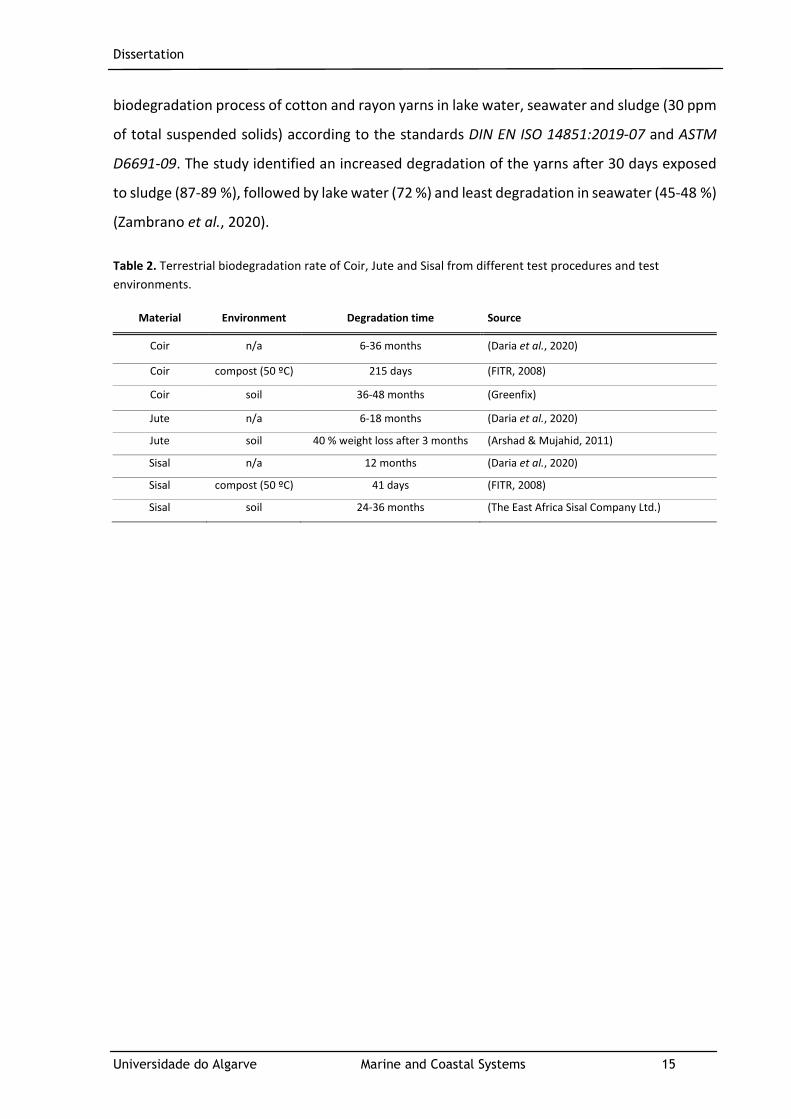
Table 2. Terrestrial biodegradation rate of Coir, Jute and Sisal from different test procedures and test
environments. ............................................................................................... 15
Table 3. Presentation of five different selected textile substrates as carrier substrates for implantation of
Zostera marina shoots and their weight and tensile strength. ............................................. 27
Table 4. Terrestrial degradation behavior of natural materials. Data based on a comprehensive review of
several studies. Hence, the individual methodologies on testing the degradation behavior vary and
therefore, degradation time varies strongly. (Daria et al., 2020) .......................................... 28
Table 5. Summary of total sample number and required burial area. ..................................... 30
Table 6. Parameters for tensile strength test procedures for textiles according to DIN EN ISO 13934-1
(ISO 13934-1:1999). ......................................................................................... 33
Table 7. General permutational MANOVA results of physical (weight loss, tensile strength loss) and
biological (OCR) descriptors of biodegradation of textile layouts, buried in the Ria Formosa lagoon with
factor Layout and time of burial. Per Layout and Time interval five replicates were buried, total n=180.
α-level=0.05, significant result presented by *. ............................................................ 45
Table 8. General permutational MANOVA results of morphological and photosynthetic parameters of
Zostera marina shoots with factors ‘Layout’ and ‘Time Interval’. Used layouts were CC,CT7,SC, ST7 along
with fertilized shoots and controls (see composition Fig. 6) Per Layout five replicates were placed into
independent mesocosms with five shoots each. Total shoot n=150. α-level=0.05, significant result
presented by *. .............................................................................................. 56
Table 9. Legend - Translation of graph labels ............................................................... 84

ABBREVATIONS
C Control
CC Coir net – Coir mat
CCMAR Center of Marine Sciences
CT7 Coir net – Type 7 mat
FT Fertilizer
JC Jute net – Coir mat
JT7 Jute net – Type 7 mat
N Nitrogen
OCR Oxygen Consumption Rate
P2O5 Phosphorus pentoxide
PAM Pulse-Amplitude-Modulation
PS I Photosystem I
PS II Photosystem II
SC Sisal net – Coir mat
SiO2 Silicon Dioxide
ST7 Sisal net – Type 7 mat
Dissertation
Universidade do Algarve Marine and Coastal Systems 1
1 INTRODUCTION AND MOTIVATION
The Intergovernmental Science-Policy Platform on Biodiversity and Ecosystem Services (IPBES)
identified that, nature is declining world-wide at an unprecedented rate. The rate of
ecosystem loss and species extinction is accelerating, resulting in severe impacts on ecosystem
services such as food security, livelihood, economy, health and more (IPBES, 2019). The
current extinction rate is 1,000 times higher compared to natural background rates and is
most likely to rise up to the 10,000 fold (Vos et al., 2015). According to IPBES, global indicators
of ecosystem extend and conditions decreased 47 % from the estimated natural baseline.
Main driver for loss of biodiversity and ecosystems are assigned to significant habitat
alteration through human activity. In between the 18th and 21st century more than 85 % of
wetlands have diminished as well as 66 % of the marine environment has been drastically
transformed up to this day.(IPBES, 2019).
Especially marine environments suffer from anthropogenic exploitation. Overfishing,
aquaculture, exploitation of resources and other coastal engineering activities contribute to
habitat changes, in a possibly even synergistical manner (Halpern et al., 2008). The majority
of human activities operate in the intertidal and nearshore zone such as marshes, mangroves,
sand beaches, dunes, seagrass beds, and coral and oyster reefs, pressuring these ecosystems
to a higher extent than the offshore regions (Halpern et al., 2008; Barbier, 2017). Terrestrial
and marine environments along with human welfare depend strongly on the ecosystem
services, provided by the coast and the high seas (Barbier, 2017) due to the profound
interconnectivity between ecological and socioeconomic systems (Margerum, 1999). Marine
systems protect coasts from storms and erosion, provide food, oil, minerals and other
resources, are used for recreational purposes, transport and pollution control (Barbier, 2017).
The decline in fish populations, for example, results in a decreased food provision (humans
and animals) and water quality, increased algae blooms, hypoxia and possibly the loss of
complete ecosystems (Barbier, 2017). Densely populated coastal regions are directly impacted
by these ecosystem losses, endangering 100-300 million people (IPBES, 2019).
The diminishing of natural environments, and thus decreases in ecosystem services for
humankind and environment, calls for protection and restoration efforts. Many systems
cannot recover themselves as efficient as through assisted action, even if stressors are
Dissertation
Universidade do Algarve Marine and Coastal Systems 2
minimized or completely removed, therefore active restoration must be emphasized (Perrow
& Davy, 2004; Rey Benayas et al., 2009). The integrity of ecosystems can be either entirely
restored, recreated and/or enhanced, depending on their initial state and the desired purpose
of restoration (Wilson & Forsyth, 2018). The success of restoration programs can be
determined by measuring the improvement of ecosystem services (Basconi et al., 2020).
A vast number of essential ecosystem services are provided by organisms such as
seagrass meadows. They provide nursery homes for juveniles or food for other organisms.
Seagrass patches are one of the most productive ecosystems in the world (Reynolds, 2013;
Descamp et al., 2017a), and are crucial for anthropogenic purposes such as protection of
beaches from erosion and sequestering carbon from the atmosphere (Descamp et al., 2017b;
Unsworth et al., 2019). However, seagrass meadows suffer from high stress and have been
constantly declining since the preindustrial times (Eriander, 2017). Over the past 130 years,
one third of worldwide seagrass meadows disappeared with a decrease of 7 % yr-1 since 1990
(Waycott et al., 2009).The diminishing of seagrass meadows can be primarily attributed to
anthropogenic stressors. These include the input of chemical loads into the system, physical
damage (dredging, mooring and propeller scars), input of increased nutrient loads and more
(Fonseca et al., 1998; Descamp et al., 2017b; IPBES, 2019). Worldwide restoration efforts have
been made since the late 1930’s (Tan et al., 2020). Especially, the United States and Australia
are well experienced in seagrass restoration and were amongst the first nations to give
attention to these ecosystems (Fonseca et al., 1998; Erftemeijer, 2020). Nevertheless, due to
the slow recovery rate of seagrasses and the low germination rate of their seeds, large scale
and long term restoration of meadows has turned out to be a difficult task and success rates
are therefore considerably low (average 37 % success rate) (Fonseca et al., 1998; Xu et al.,
2016; Eriander, 2017). Currently, a wide number of innovative methodologies and approaches
are under development and tested globally on different seagrass species at different latitudes.
Traditional and most conventional techniques of seagrass restoration include the sod, single
shoot and/or seed transplant method, including different planting and anchoring systems such
as metal frames, mussels, rocks, textile bags and strips, simple burying and more (Erftemeijer,
2020).
The main issue, arising with the application of traditional transplanting methods, is the
adverse effect on the donor meadows. Adult plants are used for transplanting efforts
Dissertation
Universidade do Algarve Marine and Coastal Systems 3
therefore, the population of the donor meadow declines for restoration efforts. Especially, in
large scale projects, existing seagrass meadows suffer from the exploitation of sods and shoots
from their system. Many times the donor meadow cannot recover from the loss due to their
slow recovery rate (Fonseca et al., 1998; Xu et al., 2016). Furthermore, various studies on
seagrass restoration report their transplantation attempts as successful, although the
monitoring periods of often less than a year are not sufficient to give reliable results (Zhou et
al., 2014). Premature meadows suffer from hydrological pressures such as waves and storm
events and often cannot withstand the disturbing forces (Paulo & Cunha et al., 2019). Beyond
that, environmental and biological factors vary within years, therefore a short monitoring
period lacks these variabilities and shoots that survived in one year might not survive the
following (Zhou et al., 2014).
Combined, these problems call strongly for the development of donor-free methods
for seagrass restoration in order to protect the donor population and additionally, provide a
carrier substrate, that can function as growing surface for the premature seagrass shoots,
therewith they can withstand the first winter storms of the year after transplantation.
This work focus on the establishment of basic knowledge on the response (survival
rate) of seagrass shoots, planted into different carrier substrates (textiles) and their ability of
the roots to entangle into substrates as well as on the performance (degradation and
mechanical strength) of these textiles in the marine environment. Solely textiles, that are fully
biodegradable, without releasing adverse by-products during degradation into the system,
were assessed experimentally. The intention was not to disturb the marine system by placing
synthetic structures into the environment and, to develop an innovative and feasible
transplanting method, which does not harm donor meadows to such an extent as traditional
transplanting does. A variety of requirements must be met for the textiles to be successful in
the field. The material needs to be resistant against permanent hydrological pressures such as
currents from tides, wave action as well as winter storms. Beyond physical pressures, the
materials must withstand microbial attacks and saline marine conditions for an extended
period. Hence, the biodegradation rate of each textile was evaluated by monitoring weight
and tensile strength loss along with aerobic microbial activity of buried textiles in the marine
environment. Moreover, the textiles must supply a matrix, which allows the roots of the
seagrass to incorporate in, thereby stabilization of the shoots in the environment can be
Dissertation
Universidade do Algarve Marine and Coastal Systems 4
assured. Shoots were incorporated into the textiles and their response monitored and
analyzed.
This work bears great potential in providing essential information on a new method for
restoration. Future studies of the project aim at the multiplication of harvested seagrass
shoots in artificial tanks and eventually, transplant the multiplied population back into the
environment. The textiles will serve as a large-scale base, which facilitates transport and
results in effortless out bedding of the new plants. Thereby, donor meadows face less
disturbances and, new shoots have sufficient time to root into the seabed due to the
stabilization by the carrier substrate
1.1 RESTORATION PROGRAMS
The unprecedent deterioration of marine ecosystems related to human activities bears
adverse effects on human welfare. Marine ecosystems provide several essential functions
with respect to food supply, coastal protection, erosion control and more. Coastal and marine
managers face the challenge on sustaining and restoring these ecosystems to assure security
for humankind. Artificial solutions, such as groins and jetties have been used to control the
degradation of these ecosystems, however these man-made solutions fall short in resiliency
and may further complicate the status of the nearby ecosystem along with generating
exorbitant costs (Ferrario et al., 2014). Recently focus has been set on so-called ecosystem
engineers such as corals, mangroves, seagrasses and others. These organisms modify their
abiotic environment and create favorable abiotic and biotic conditions for other species and
men (Jones et al., 1994; Rossi et al., 2013; Basconi et al., 2020). Ecosystem engineers are a
cost-effective option for restoration programs of ecosystem services (Byers et al., 2006).
However, these organisms are part of the diminishing ecosystem and therefore, lose their
ability to protect and sustain ecosystem services (Rossi et al., 2013). Consequently, ecosystem
engineers can either be newly introduced into a system or, more importantly, conserved and
restored where they already exist in order to reestablish and maintain their supporting impact
on their environment (Law et al., 2017).
According to Basconi et al., (2020) restoration ecology gained strong interest in the
past two decades. The intention of this emerging scientific branch is to rehabilitate
Dissertation
Universidade do Algarve Marine and Coastal Systems 5
ecosystems in comparison to a historical baseline. Hence, it aims at habitats, in which the
ecosystem of concern was present beforehand and suffered damage and loss. In order to
succeed, Bayraktarov et al., (2016) suggest four criteria, that must be considered; (1)
understanding of the functions of the ecosystems, (2) removal of anthropogenic disturbances,
(3) clearly defined success evaluation, (4) long term monitoring > 5 years (approx. 15-20
years). Different restoration techniques have been developed, ranging from planting juveniles
to adult organisms, collected from a donor site, or the introduction of artificial structures,
hosting the target species (Basconi et al., 2020). During an analysis of 235 articles on marine
restoration programs conducted by Bayraktarov et al., (2016) the main target species, costs
as well as main challenges with respect to rehabilitation actions were identified. Ecosystems
from most interest for restoration purposes include salt marshes, coral reefs, oyster reefs,
seagrass meadows and mangroves. Costs range widely depending on methodology and
resources. Estimated costs can range from US$ 2.508/ha for mangrove restoration up to
US$ 383,672/ha for seagrass restoration (Bayraktarov et al., 2016). According to Bayraktarov
et al., (2016) total restoration costs appear not to increase with expansion of the project scale
in regard to coral reef and seagrass meadow restoration. Though, most projects were
conducted on a small scale; <1 ha and <10 ha, for coral reef and seagrass respectively,
wherefore the estimation might not be accurate (Bayraktarov et al., 2016). The least
successful (38 % success rate), but at the same time one of the most cost-intensive programs
is related to seagrass (Bayraktarov et al., 2016), therefore already existing approaches must
be improved or new innovative strategies must be developed.
1.2 SEAGRASSES: BIOLOGY AND DISTRIBUTION
Seagrasses are aquatic plants, distributed throughout shallow marine systems around the
world, from the Southern Hemisphere to tropical regions up to the Arctic (Reynolds, 2013).
They are angiosperms (flowering plants) and inhabit coastal areas from the intertidal up to
depths excess of 50 m (Duarte, 2001; Reynolds, 2013; Encyclopedia Britannica, 2020).
Seagrasses are further categorized as monocotyledons (angiosperms), implying they possess
one embryonic leaf in their seeds (Encyclopedia Britannica, 2020).
There are 72 species of seagrasses identified, assigned to four main taxonomic groups;
Zosteraceae, Hydrocharitaceae, Posidoniaceae and Cymodoceaceae (Reynolds, 2013).
Dissertation
Universidade do Algarve Marine and Coastal Systems 6
According to Short et al., (2007) species are distributed to different extent throughout the six
global bioregions: Temperate North Atlantic, Temperate North Pacific, Mediterranean,
Temperate Southern Oceans, Tropical Atlantic, Tropical Indo-Pacific. The Temperate North
Atlantic features an overall low species diversity and is dominated by the species Zostera
marina, which grows predominantly in estuaries and lagoons. Extensive species diversity can
be found in the estuarine and surf zones of the Temperate North Pacific including species of
Zostera spp. and Phyllospadix spp..Closer towards low latitudes, the Mediterranean waters
host a modest amount of different seagrasses including temperate and tropical species,
dominated by Posidonia oceanica. The Temperate Southern Oceans are habitat to a vast
number of seagrass meadows ranging from low to high diversity temperate seagrasses.
Posidonia and Zostera dominate this area. The highest biodiversity of seagrass species can be
found in the tropical regions of the Indo-Pacific as well as the Tropical Atlantic, both
dominated by Thalassia testudinum. (Short et al., 2007; Eriander et al., 2016)
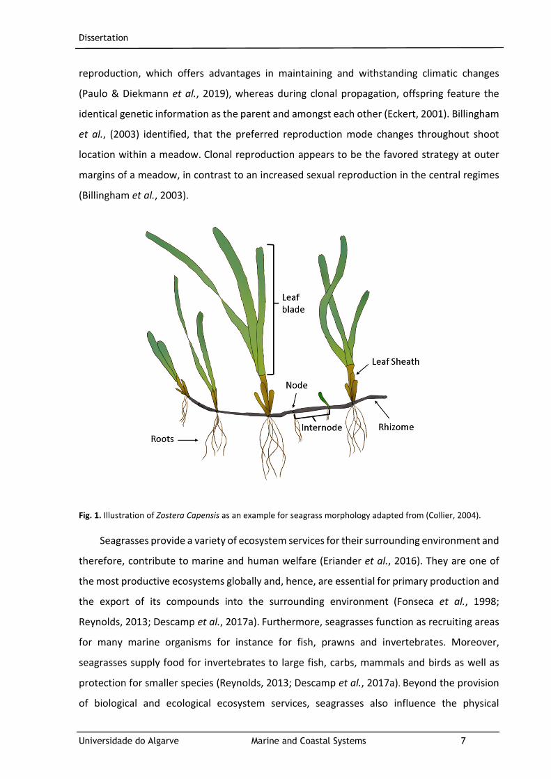
The morphology of seagrasses can be divided into above and below ground parts (Fig.
1). According to the definition of Kuo & Hartog, (2006) above ground, multiple elongated
leaves are embraced in shoots. A basal sheath wraps each leaf, protecting the apical meristem.
Sugar production via photosynthesis occurs in the distal blade as well as transpiration of water
vapor. Above ground parts are characterized by three tissues; the epidermis as a surface layer,
regulating transpiration and aeration together with provision of mechanical support, the
vascular bundle, which contains the phloem and the xylem, responsible for organic and
inorganic solute transport and the parenchyma tissue, controlling photosynthesis and storage.
Below ground parts anchor the seagrass to the seabed and include roots, rhizomes and in
some cases erected stems, which together construct a widely interconnected underground
system. Roots, shoots and stems are connected to the creeping rhizomes at each node or
every other node. Additional to the mechanical support, the rhizomes provide essential
functions for regulation and maintenance of seagrass growth, including the storage of
nutrients. During sexual reproduction seagrasses develop flowers, which produce seeds for
pollination and fertilization. (Kuo & Hartog, 2006)
Seagrasses produce offspring either asexually by growing new rhizomes and thus,
producing new shoots or sexually by the transport of male pollen through the water, fertilizing
female flowers and producing seeds (Reynolds, 2013). Genotypic diversity is assured via sexual
Dissertation
Universidade do Algarve Marine and Coastal Systems 7
reproduction, which offers advantages in maintaining and withstanding climatic changes
(Paulo & Diekmann et al., 2019), whereas during clonal propagation, offspring feature the
identical genetic information as the parent and amongst each other (Eckert, 2001). Billingham
et al., (2003) identified, that the preferred reproduction mode changes throughout shoot
location within a meadow. Clonal reproduction appears to be the favored strategy at outer
margins of a meadow, in contrast to an increased sexual reproduction in the central regimes
(Billingham et al., 2003).
Fig. 1. Illustration of Zostera Capensis as an example for seagrass morphology adapted from (Collier, 2004).
Seagrasses provide a variety of ecosystem services for their surrounding environment and
therefore, contribute to marine and human welfare (Eriander et al., 2016). They are one of
the most productive ecosystems globally and, hence, are essential for primary production and
the export of its compounds into the surrounding environment (Fonseca et al., 1998;
Reynolds, 2013; Descamp et al., 2017a). Furthermore, seagrasses function as recruiting areas
for many marine organisms for instance for fish, prawns and invertebrates. Moreover,
seagrasses supply food for invertebrates to large fish, carbs, mammals and birds as well as
protection for smaller species (Reynolds, 2013; Descamp et al., 2017a). Beyond the provision
of biological and ecological ecosystem services, seagrasses also influence the physical

Dissertation
Universidade do Algarve Marine and Coastal Systems 8
environment positively for humans by securing lose sediment from the seabed via their widely
distributed underground root and rhizome system, inhibiting erosion of beaches and
controlling sediment flow (Fonseca et al., 1998; Descamp et al., 2017b). Furthermore,
hydrodynamics and wave height can be reduced by more than 36 %, contributing to coastal
protection (Narayan et al., 2016). Additionally, seagrasses can be a useful tool for
management purposes such as water quality assessment and improvement (Fonseca et al.,
1998) by trapping fine particles in and therefore, cleaning the water column (Eriander et al.,
2016; Narayan et al., 2016). Beyond the direct influence of the seagrasses on the marine
environment, they also affect the atmosphere in a beneficial manner. Seagrasses are
considered a blue carbon storage, due to their ability to sequester atmospheric carbon and
store it in the soil, accounting for10–18 % of global carbon burial in the marine environment
(Röhr et al., 2018; Unsworth et al., 2019; Bedulli et al., 2020). A recent study from Bedulli et
al., (2020) (Bedulli et al., 2020)(Bedulli et al., 2020)conducted on Rottnest Island, Australia,
even identified an approximately storage capacity from mixed seagrass populations of 22 %
of the island’s carbon dioxide emissions (Bedulli et al., 2020). These studies prove that
seagrasses can play a key role in fighting anthropogenic induced CO2.
The importance of seagrass meadows for assuring socioecological security requires
intensified conservation and restoration actions of these ecosystems.
1.3 MODEL SPECIES: ZOSTERA MARINA
Zostera marina, also known as “common eelgrass”, is the most dominant angiosperm species
throughout the Northern Hemisphere, distributed from the Arctic down to the warm waters
of the Mediterranean Sea (Fig. 2) (Setchell, 1935; Borum et al., 2004; Eriander et al., 2016). It
populate the intertidal as well as subtidal (10-15 m depth), determined by water clarity and
light penetration (Borum et al., 2004; Short et al., 2007). Populations differ in their
morphology, with increasing size towards higher latitudes, in their tolerance to temperature
and salinity as well as in their lifecycle, confirmed by occurrences of perennial, biennial and
annual populations (Larkum et al., 2006; Short et al., 2007).
Zostera marina (Fig. 2) predominantly grows in monospecific meadows and varies
seasonally in biomass production, shoot density and morphology (Solana-Arellano et al., 1997;

Dissertation
Universidade do Algarve Marine and Coastal Systems 9
Borum et al., 2004; Short et al., 2007). It is composed of three to seven leaves per shoot, which
feature a width of 2 mm to 10 mm and an average length between 30 to 60 cm, depending on
their maturity status. Shoots are connected to below ground rhizomes, which form a new
rhizome segment (internode) for each new leaf along with 2 - 20 cm long root bundles on each
node. Flowering occurs during spring to fall and 2-4 mm long seeds develop, which distribute
by either floating away with the detached shoots or fall to the nearby ground within the same
meadow (Borum et al., 2004).
Fig. 2. Zostera marina distribution (left), adapted from (Borum et al., 2004) and scheme of Zostera marina
morphology (right) (Fonseca et al., 1998).
Zostera marina populations have suffered strongly from variations in abundancy
throughout the last century. In the 1930’s almost the complete population (90 %) in the
Northern Atlantic has been diminished due to an epidemic disease known as the saprophytic
net slime mold, Labyrinthula spp. (TUTIN, 1938; Ralph & Short, 2002; Keser et al., 2003).
Beyond that, long term decline in Zostera marina populations has been attributed to
anthropogenic disturbances in e.g. Rhode Island, United States (Short et al., 1996). Particularly
increasing eutrophication is detrimental to the high light requiring species of Zostera marina
due to its reducing effect on water clarity and therefore, light attenuation (Dennison et al.,
1993; Eriander, 2016). Additionally, eelgrass lacks the ability to re-establish itself once
destroyed in a larger scale even if, pressures are minimized or eliminated (Boström et al.,
Dissertation
Universidade do Algarve Marine and Coastal Systems 10
2014). The vast decline of eelgrass meadows and the inability to recover on their own, leaves
them one of the most endangered and vulnerable ecosystem worldwide(Dennison et al.,
1993; Waycott et al., 2009; Boström et al., 2014).
Zostera marina was identified as the most threatened species along the Portuguese
coast, impacted by bivalve hand trawling, boat mooring and channel dredging (Cunha et al.,
2013). Meadows of this species are abundant in only two sites in Portugal; Lagoa de Óbidos
and the Ria Formosa Lagoon, covering a total area of 0.075km2 (Cunha et al., 2013).The Ria
Formosa Lagoon in the south of Portugal accommodates 42 meadows of Zostera marina,
which account for an area of 5.01 ha (Cunha et al., 2009). Restoration efforts of Zostera in
other regions of the country such in the Arrábida national park were subject to failure (Cunha
et al., 2013).
1.4 NATURAL FIBERS
Natural fibers are gaining increased popularity in the field of geotextiles, especially attributed
to their green biodegradation (Ghosh et al., 2017; Wu et al., 2020). As of today, according to
Wu et al., (2020), geotextiles made of natural fibers have the ability to replace 50 % of the
synthetic products on the market (Wu et al., 2020).
Natural fibers can be divided into three categories: plant fibers, animal fibers and
mineral fibers. Plant fibers are the most favorable fiber, due to their low cost in sourcing and
processing as well as their superior mechanical performance (Wu et al., 2020).The three main
components of plant fibers are cellulose, hemicellulose and lignin, whose weight proportion
determines the physical properties of the fibers (Table 1) (Wu et al., 2020).
Textiles offer a wide range of applications and are often found in the geotechnical
sector (Wu et al., 2020). These so-called geotextiles are commonly produced from
petrochemical derivates (Wu et al., 2020). Nowadays the demand for green geotextiles is
rising and where applicable preferred (Mahuya et al., 2009; Wu et al., 2020). Green geotextiles
are composed from natural fibers and have no adverse effect on the environment (Mahuya et
al., 2009). Among plant fibers jute and coir convince with their outstanding mechanical
performance, hence are used in this branch (Mahuya et al., 2009). Sisal fibers feature

Dissertation
Universidade do Algarve Marine and Coastal Systems 11
distinctive seawater resistance and are prominent materials for maritime applications such as
ropes and nets (Mukherjee & Satyanarayana, 1984).
Table 1. Composition and properties of natural fibers commonly used to make natural geotextiles, (Koohestani
et al., 2019; Wu et al., 2020).
Type of
Fiber
Cellulose
(wt%)
Lignin
(wt%)
Hemicellulose
(wt%)
Density
(g/m3)
Strain at Break
(%)
Tensile
Strength
(Mpa)
Young’s
Modulus
(Mpa)
Flax 71-78 2.2 18.6-20.6 1.4-1.5 1.2-3.2 345-1500 27.6-80
Hemp 57-77 3.7-13 14-22.4 1.48 1.6 550-900 70
Jute 45-71.5 12-26 13.6-21 1.3-1.46 1.5-1.8 393-800 10-30
Kenaf 31-57 15-19 21.5-23 1.2 2.7-6.9 295-930 22-60
Ramie 68.6-76.2 0.6-0.7 5-16.7 1.5 2-3.8 220-938 44-128
Nettle 86 5.4 4 1.51 1.7 650 38
Sisal 47-78 7-11 10-24 1.33-1.5 2-14 400-700 9-38
Abaca 56-63 7-9 21.7 1.5 2.9 430-813 33.1-33.6
Cotton 85-90 0.7-1.6 5.7 1.21 3-10 287-597 5.5-12.6
Coir 36-43 41-45 0.15-0.25 1.2 15-30 175-220 4-6
Source: (Koohestani et al., 2019; Wu et al., 2020)
1.4.1 COIR (COCONUT)
Coconut fibers (Cocos nucifera) are considered fruit/seed fibers, which are obtained from the
surrounding husk of the coconut (Satyanarayana et al., 1981; Ramamoorthy et al., 2015). Palm
trees take up 10 million ha of land throughout the tropical regions, making coir fibers an easily
accessible, economic and renewable resource (LEKHA & KAVITHA, 2006; Lal et al., 2017; Bui
et al., 2020). The Food and Agriculture Organization of the United Nations FAO elaborated the
five nations that contribute to 90 % of the global coir fiber production (0.78 million tons/year;
(Satyanarayana et al., 1981), which are India, Sri Lanka, Thailand, Vietnam, and Philippines
(Bui et al., 2020). The application of these fibers reaches from ropes over mattresses and
geotextiles to automobile seats and more (Bui et al., 2020).
The multicellular coir fiber1 features a polygonal or round cross section (diameter
approx. 0.3 mm) and fiber length ranges between 5 to 350 mm on average (Satyanarayana et
al., 1981; Lekha, 2004; Daria et al., 2020). The fibers consists mainly of 36-43 % of cellulose
1 30 to 300 or more cells in the total cross-section of the coir fiber Satyanarayana et al. (1981)
Dissertation
Universidade do Algarve Marine and Coastal Systems 12
and 0.15-0.25 % of hemicellulose with a lignin content of 41-46 %, being the highest lignin
content found in all natural fibers (Lekha, 2004; Daria et al., 2020). Further components are
pectin (2.75-4 %) and water solubles (Satyanarayana et al., 1981; Lekha, 2004). The high
density of these fibers leaves them more durable than other natural fibers such as jute and
sisal (Lekha, 2004; Daria et al., 2020). The increased lignin percentage gives the fiber the
advantage of lower water absorption capacity, hence increasing its resistance towards
microbial attack as well as higher resistance towards elongation (Sumi et al., 2018; Daria et
al., 2020). Most important, coconut fibers feature resistance towards seawater and are
utilized e.g. in the control of sea-erosion (Satyanarayana et al., 1981) or other applications in
maritime engineering (Ramamoorthy et al., 2015; Daria et al., 2020). The main disadvantage
of this fiber is its low tensile strength, which can be only improved via specific physical and
chemical treatments (Ramamoorthy et al., 2015; Bui et al., 2020; Daria et al., 2020).
1.4.2 JUTE
Jute fibers are considered bast fibers, which are won from the stem of the Corchorus
capsularis/ Corchorus olitorius, making them one of the most low-cost natural fibers (Singh et
al., 2018). The plants are mainly grown for their fiber, since they are cheap to cultivate and
process. Furthermore, their annual growth pattern results in vast material supply
(Ramamoorthy et al., 2015; Singh et al., 2018). The global annual production accounts for
2300 x 103– 2850 x 103 tons, which for the most part comes from India, China, Bangladesh,
Nepal, Thailand, Indonesia, and Brazil (Ramamoorthy et al., 2015; Singh et al., 2018). Mean
fiber length accounts for 2.5 mm (Alloftextiles Online Limited, 2015). The reported chemical
composition varies slightly amongst studies. According to Ramamoorthy et al., (2015) and
Daria et al., (2020) cellulose content ranges between 56-71.5 %. Reported values for
hemicellulose lie between 29-35 % and for lignin 11-14 %. Despite the low resistance of jute
fibers against moisture, acid and UV light (Singh et al., 2018) they perform sufficiently in
geotechnical applications at low cost such as consolidation, drainage, soil filtration, road
construction, stabilization and protection of slopes, and erosion control (Datta, 2007;
Chattopadhyay & Chakravarty, 2009; Daria et al., 2020). Jute fiber are prone to degrade rapidly
in saltwater (Daria et al., 2020). However, studies have not been performed in marine
environment but only laboratory conditions, therefore the fiber’s behavior in realistic
conditions will be assessed in this research.
Dissertation
Universidade do Algarve Marine and Coastal Systems 13
1.4.3 SISAL
Sisal fibers are categorized as hard fibers, harvested from the leaves of the agave sisalana
plant (Ramamoorthy et al., 2015). The total fiber production worldwide accounts for
approximately 4.5 million tons per year, mainly cultivated in Tanzania and Brazil, but also
found in China and Kenya (Chand et al., 1988; Ramamoorthy et al., 2015). Sisal fibers are
utilized for ropes and twines and chords, especially for marine and agricultural purposes as
well as for upholstery, padding, fish nets and decorative articles (Li et al., 2000; Ramamoorthy
et al., 2015). Values for the chemical composition of the fiber vary strongly amongst source
and age of the plant (Li et al., 2000). According to Li et al., (2000) the cellulose content ranges
between 49.62-60.95 %, and the lignin content from 3.75-4.40 %. Differing values are reported
from Ramamoorthy et al., (2015) with a range of 67-78 % and 8-11 %, respectively. The fiber
length is between 1.0 and 1.5 m and the diameter around 100-300 μm (Li et al., 2000). Sisal
fibers feature a high tensile strength and are robust against deterioration in saltwater, making
them suitable for this study (Haque et al., 2015).
1.5 BIODEGRADATION TEXTILES IN MARINE ENVIRONMENT
The term ‘biodegradable’ must be clearly defined. Illustrated by Endres & Siebert-Raths,
(2009) there are two steps taking place during degradation. Primary degradation implies the
splitting of macro-molecules of a material by microorganisms into smaller particles. The
decomposition products are subsequently converted into H2O and CO2 enzymatically,
resulting in the final decomposition and, can be absorbed by the microorganisms. If a material
cannot be decomposed completely it cannot be considered biodegradable. External
conditions such as time, temperature and humidity influence the efficiency of biodegradability
(Deutsches Institut für Normung e.V.; Endres & Siebert-Raths, 2009).
Biodegradability tests do not follow a standard test procedure. The understanding and
test methods of biodegradability relate to the field of application such as wastewater
treatment or biodegradation in marine environments and can vary strongly. Timescale and
decomposition stage are not defined, hence the term ‘biodegradability’ can result in
misleading assumptions (Harrison et al., 2018b). Arshad & Mujahid, (2011) categorizes
Dissertation
Universidade do Algarve Marine and Coastal Systems 14
biodegradability in three stages of the progression of decomposition (Arshad & Mujahid, 2011;
Harrison et al., 2018a):
1. Biodeterioration stage = depolymerization by enzymic hydrolysis or peroxidation
of carbon chain polymers; mass loss and loss of mechanical properties (mass
loss > 90 % assumed to be degraded)
2. Bio fragmentation stage = disintegration and fragmentation without significant
gas evolution
3. Microbial assimilation stage = digestion of low molecular weight species = gas
evolution and mineralization
Biobased fibers can be composed of natural fibers like animal or plant fibers or
synthetic fibers, which are spun from starch, lipids, sugar and other extracted compounds
derived from plants and other natural resources (Thyavihalli Girijappa et al., 2019). Despite
the biological origin of a fiber, fully biodegradation is not granted (Siracusa, 2019). Especially
biosynthetics often do not undergo all three stages of biodegradation in a natural
environment (Siracusa, 2019). Therefore, in this study we focus on solely natural fibers,
therewith no harmful byproducts are released in the environment.
Several studies on the terrestrial biodegradation of natural fibers have been conducted
in laboratory condition as well as in the natural environment. A widely used standardized test
procedure is the so-called Soil Burial Test (DIN EN ISO 11721-1:2001) applied to natural and
synthetic fibers (Arshad & Mujahid, 2011; Sülar & Devrim, 2019) along with the standard test
procedure on biodegradation via composting (DIN EN 13432:2000-12) (FITR, 2008).
Nevertheless, data on material degradation rate vary strongly within studies and cannot be
directly compared due to modifications of the test procedures and differences in reporting
(Table 2).
Information on the biodegradability rate of natural fibers in the marine environment
is lacking. Public and socioeconomic interest lie in the behavior of synthetic fibers in marine
systems primarily, due to the release of synthetic microfibers into aquatic environments
during clothes laundering as well as the utilization of synthetic geotextiles (Dilkes-Hoffman et
al., 2019). Only recently, a study from Zambrano et al., (2020) drew attention to the
Dissertation
Universidade do Algarve Marine and Coastal Systems 15
biodegradation process of cotton and rayon yarns in lake water, seawater and sludge (30 ppm
of total suspended solids) according to the standards DIN EN ISO 14851:2019-07 and ASTM
D6691-09. The study identified an increased degradation of the yarns after 30 days exposed
to sludge (87-89 %), followed by lake water (72 %) and least degradation in seawater (45-48 %)
(Zambrano et al., 2020).
Table 2. Terrestrial biodegradation rate of Coir, Jute and Sisal from different test procedures and test
environments.
Material Environment Degradation time Source
Coir n/a 6-36 months (Daria et al., 2020)
Coir compost (50 ºC) 215 days (FITR, 2008)
Coir soil 36-48 months (Greenfix)
Jute n/a 6-18 months (Daria et al., 2020)
Jute soil 40 % weight loss after 3 months (Arshad & Mujahid, 2011)
Sisal n/a 12 months (Daria et al., 2020)
Sisal compost (50 ºC) 41 days (FITR, 2008)
Sisal soil 24-36 months (The East Africa Sisal Company Ltd.)

Dissertation
Universidade do Algarve Marine and Coastal Systems 16

Dissertation
Universidade do Algarve Marine and Coastal Systems 17
2 RESEARCH OBJECTIVE
The main goal of this work is to generate basic knowledge for the development of a feasible
and large-scale solution for seagrass restoration, based on the utilization of textiles. This is
achieved by identifying suitable materials and textile structures, used as a carrier base for
seagrass shoot transplants. The fabrics act as an anchoring device for roots and rhizomes of
seagrasses to entangle in and hence, shoots can overcome heavy storm events until they are
fully capable to withstand hydrological pressures. The model seagrass of this work is the in the
Northern Hemisphere most dominant seagrass species Zostera marina.
Two main objectives were pursued in this study in order to acquire a suitable material
selection for seagrass restoration studies.
1. To investigate the performance over time of the different textile substrates in
regard to durability and physical properties after extended exposure to the
marine environment.
i. Burial of six different textile layouts in the intertidal of the Ria Formosa
Lagoon and retrieval after set time intervals in order to assess:
a. Weight loss over time
b. Tensile strength loss over time
c. Aerobic microbial activity
2. Assessment of Zostera marina response to the incorporation into the textiles in
a mesocosm
ii. Replicates of five seagrass shoots were inserted in each of the textiles and
placed in independent mesocosms in order to examine:
a. Survival rate
b. Plant and root morphology

Dissertation
Universidade do Algarve Marine and Coastal Systems 18
Dissertation
Universidade do Algarve Marine and Coastal Systems 19
3 STATE OF THE ART
3.4 RESTORATION AND CREATION OF SEAGRASS MEADOWS
Restoration efforts of seagrass meadows have been made around the world for over seventy
decades, with emerging interest from the 1970’s on (van Katwijk et al., 2016). The majority of
the reported studies since the 70’s were conducted in the temperate and subtropical latitudes
of the Northern Hemisphere (68 %) (van Katwijk et al., 2016). Numerous species with various
morphologies were used in the trials, Zostera marina being the most popular (50 %). Most
studies were conducted in developed countries such as United States, Australia and Europe
(van Katwijk et al., 2016). Especially in the United States high expertise in seagrass restoration
has been developed, since it was initiated there already in the 1940’s (Fonseca et al., 1998) in
conjunction with the longest restoration program of 48 years (planted in 1973, Florida) (van
Katwijk et al., 2016). Another lucrative example is the four decade long, large scale restoration
program of Zostera marina in Chesapeake Bay, USA (Fonseca et al., 1998; Erftemeijer, 2020)
along with the restoration of Posidonia australis and P. sinuosain in Oyster Bay, Australia,
convincing with high long term survival rate of over 90 % (Bastyan & Cambridge, 2008). In
contrast, nations in tropical latitudes lack knowledge and experience and awareness on
conservation and rehabilitation matters is just gaining political and socioeconomical interest
in present days (Eriander et al., 2016; Erftemeijer, 2020).
Transplanting strategies for seagrasses can be divided into traditional transplanting
methods, in which mature plants are used as donors, and seed germination, a more recent
approach (Eriander et al., 2016; Erftemeijer, 2020). Traditional restoration methods can be
subdivided into sediment and sediment-free methods (Fig. 3). One approach, including
sediments, is the plug method. Here, donor seagrasses, including attached sediments, are
collected in tubes and transported to the restoration site (Fonseca et al., 1998; Riniatsih et al.,
2018). Another approach is, to dig up a shovel of sediments including shoots and transplant
the whole sod with shoots, sediment and benthic fauna all together (so-called sod/turf
technique). Various variations of the sod method have been established, adapted to the in
situ environments (Erftemeijer, 2020). Sediment-free methods are e.g., the staple method,
which promises high success rates, though, is labor intensive, as it requires SCUBA diving.

Dissertation
Universidade do Algarve Marine and Coastal Systems 20
Shoots, roots and rhizomes are collected, while sediments are removed, and subsequently
stapled onto the seabed. Various devices can be used for anchoring the plants like shells,
Fig. 3. Sediment and sediment-free methods of seagrass transplantation. (1) Sod method on the left and two
types of the plug method in the middle and right. (2) Hessian bag transplant of shoots (3) Seagrass shoots tied
to metal frame (4) Staple method (5) Staple method. Placing staples into sediment. (Erftemeijer, 2020).
stones and rods (Erftemeijer, 2020). In order to decrease costs, an improved version of this
method, so called Transplanting Eelgrass Remotely with Frame Systems (TERFS), was created,
in which a metal frame, together with anchored shoots, is submerged. However, the metal
frame must be retrieved after some time (Park & Lee, 2007). Another technique, which holds
high innovative potential was tested in Kenya and Western Australia. Shoots were attached to
sand filled hessian bags, which served as stabilization for root and rhizome growth and
subsequently submerged (UNEP-Nairobi Convention/WIOMSA). Beyond the traditional
methods, various attempts on seed transplantation have been made. Seeds are collected from
fertile shoots and stored in tanks for several weeks until seeds accumulate on the bottom of
the tank. Eventually, the seeds can be released into the aquatic system via different methods
(1) (2)
(3) (4) (5)
Dissertation
Universidade do Algarve Marine and Coastal Systems 21
such as burying, placed into hessian bags etc. (Christensen et al.; Fonseca et al., 1998;
Unsworth et al., 2019; Erftemeijer, 2020).
Suitable practice and donor meadow are selected for the individual restoration programs,
based on environmental conditions and the economical/financial resources. Latitude, tidal
regime, grain size, water depths, salinity are factors, that must be taken into consideration
during the decision process. Exemplary, in intertidal zones access is simple and the staple
technique can be a convenient solution without increased logistical efforts, whereas
transplantation of seagrasses in deep subtidal waters may require SCUBA diving or the
submerging of frames with attached shoots in order to be more cost-effective. (Erftemeijer,
2020)
Additional to the choice of planting methodology, site selection plays an essential role in
restoration success (van Katwijk et al., 2016). Protection from severe hydrodynamical activity,
light availability and acceptable water quality, free from deterioration, are the minimum
requirements for prosperous transplanting (Bayraktarov et al., 2016; van Katwijk et al., 2016).
3.5 RISK AND PROBLEMS OF CONVENTIONAL METHODS
State-of-the-art restoration methods predominantly depend on adult plants as donor
material, collected from native meadows (Basconi et al., 2020). However, an increased
withdrawal of individual units from a meadow impedes the functionality of a holistic system,
resulting in increased vulnerability of the meadow towards biotic and abiotic stressors. Patchy
meadows, with increased margins, are more likely to be subject of increased grazing activities
of herbivores, whereas dense meadows rather function as nursery than nourishment (Statton
et al., 2015). Moreover, changes in the spatial distribution of seagrass meadows alter the
provision of ecosystem services such as the sequestration of carbon from the atmosphere.
Stocks were found to be 20 % higher in the meadow’s interior, in contrast to lower stocks at
the edges and bare patches (Ricart et al., 2015). Decrease in meadow density, furthermore,
gives opportunity to fast-growing invasive species to colonize within the meadow, resulting in
competition and disruption (Williams, 2007; Cullen-Unsworth & Unsworth, 2016).
Beyond selection of appropriate methodology, scientists have been facing the
challenge of evaluating and quantifying restoration success. Conventionally, success rate has
Dissertation
Universidade do Algarve Marine and Coastal Systems 22
been measured on the mortality of the transplants, nevertheless the variety of used metrics
leads to profound differences in the assessment of success, resulting in biased reporting
(Basconi et al., 2020). Biased reporting is further nurtured through the pressure put on the
scientific community from stakeholders and regulators to publish successful results,
withdrawing the opportunity for follow up research to improve from already made mistakes
(Zedler, 2007).
Amongst the challenges in assuring non-biased reporting, the monitoring intervals as
well as duration of restoration programs play a key role (Basconi et al., 2020). Most
transplanting programs undergo irregular and short monitoring periods, thereby making the
program appear successful. Consequently, in reality failed programs cannot be detected and,
opportunities for improvement dissipate (Tan et al., 2020). Unfortunately, many shoots do not
survive in the long term and the success rate of transplanting studies might even result in a
negative balance, due to the harm induced on the donor population and the loss of the newly
transplanted meadow due to storm events or other environmental/biological factors (Cunha
et al., 2012; Tan et al., 2020). In order to enhance resilience and long term success of the
restoration site, small scale trials must be translated into large scale programs, which has been
challenging up to present day (van Katwijk et al., 2016).
In particular logistics can bear challenges, often resulting in high costs. Obstacles,
summarized in the UNEP Nairobi Convention, include e.g., the high weight of sediments and
shoots, collected using the sod method, complicating transport and transplanting. Sediment-
free methods are very labor intensive due to the cleaning of roots and rhizomes from
sediments and the individual transplanting of the shoots, which may require SCUBA diving.
Difficulties deriving using seed transplanting is the low germination rate of the seeds, which
accounts for approximately 5 – 10 %. Additionally, seeds might be transported far away from
the original transplanting site through currents or get eaten by predators, decreasing the
chances of successful restoration (Erftemeijer, 2020). Crucial is, that in the majority of cases
the transplantation rate cannot compete with the mortality rate, amplifying the importance
of finding large-scale restoration solutions (Fonseca et al., 1998).
Textiles appear as a cost-effective solution, offering the opportunity of large-scale
deployment. They are applicable for seed transplanting techniques as well as growing surface
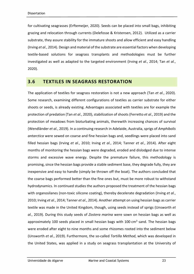
Dissertation
Universidade do Algarve Marine and Coastal Systems 23
for cultivating seagrasses (Erftemeijer, 2020). Seeds can be placed into small bags, inhibiting
grazing and relocation through currents (Delefosse & Kristensen, 2012). Utilized as a carrier
substrate, they assure stability for the immature shoots and allow efficient and easy handling
(Irving et al., 2014). Design and material of the substrate are essential factors when developing
textile-based solutions for seagrass transplants and methodologies must be further
investigated as well as adapted to the targeted environment (Irving et al., 2014; Tan et al.,
2020).
3.6 TEXTILES IN SEAGRASS RESTORATION
The application of textiles for seagrass restoration is not a new approach (Tan et al., 2020).
Some research, examining different configurations of textiles as carrier substrate for either
shoots or seeds, is already existing. Advantages associated with textiles are for example the
protection of predation (Tan et al., 2020), stabilization of shoots (Ferretto et al., 2019) and the
protection of meadows from bioturbating animals, therewith increasing chances of survival
(Wendländer et al., 2019). In a continuing research in Adelaide, Australia, sprigs of Amphibolis
antarctica were sewed on coarse and fine hessian bags and, seedlings were placed into sand
filled hessian bags (Irving et al., 2010; Irving et al., 2014; Tanner et al., 2014). After eight
months of monitoring the hessian bags were degraded, eroded and dislodged due to intense
storms and excessive wave energy. Despite the premature failure, this methodology is
promising, since the hessian bags provide a stable sediment base, they degrade fully, they are
inexpensive and easy to handle (simply be thrown off the boat). The authors concluded that
the coarse bags performed better than the fine ones but, must be more robust to withstand
hydrodynamics. In continued studies the authors proposed the treatment of the hessian bags
with organosilanes (non-toxic silicone coating), thereby decelerate degradation (Irving et al.,
2010; Irving et al., 2014; Tanner et al., 2014). Another attempt on using hessian bags as carrier
textile was made in the United Kingdom, though, using seeds instead of sprigs (Unsworth et
al., 2019). During this study seeds of Zostera marina were sown on hessian bags as well as
approximately 100 seeds placed in small hessian bags with 100 cm3 sand. The hessian bags
were eroded after eight to nine months and some rhizomes rooted into the sediment below
(Unsworth et al., 2019). Furthermore, the so-called Tortilla Method, which was developed in
the United States, was applied in a study on seagrass transplantation at the University of
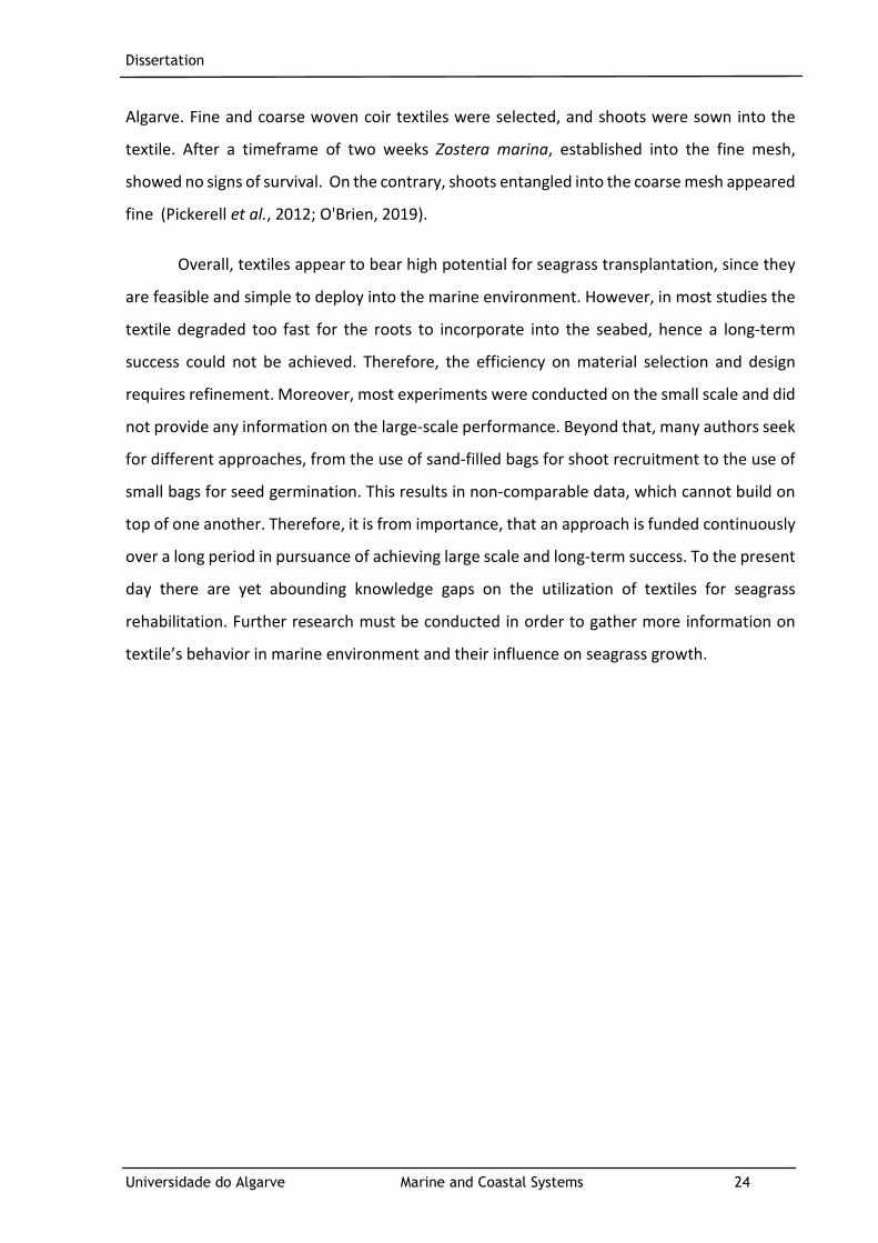
Dissertation
Universidade do Algarve Marine and Coastal Systems 24
Algarve. Fine and coarse woven coir textiles were selected, and shoots were sown into the
textile. After a timeframe of two weeks Zostera marina, established into the fine mesh,
showed no signs of survival. On the contrary, shoots entangled into the coarse mesh appeared
fine (Pickerell et al., 2012; O'Brien, 2019).
Overall, textiles appear to bear high potential for seagrass transplantation, since they
are feasible and simple to deploy into the marine environment. However, in most studies the
textile degraded too fast for the roots to incorporate into the seabed, hence a long-term
success could not be achieved. Therefore, the efficiency on material selection and design
requires refinement. Moreover, most experiments were conducted on the small scale and did
not provide any information on the large-scale performance. Beyond that, many authors seek
for different approaches, from the use of sand-filled bags for shoot recruitment to the use of
small bags for seed germination. This results in non-comparable data, which cannot build on
top of one another. Therefore, it is from importance, that an approach is funded continuously
over a long period in pursuance of achieving large scale and long-term success. To the present
day there are yet abounding knowledge gaps on the utilization of textiles for seagrass
rehabilitation. Further research must be conducted in order to gather more information on
textile’s behavior in marine environment and their influence on seagrass growth.
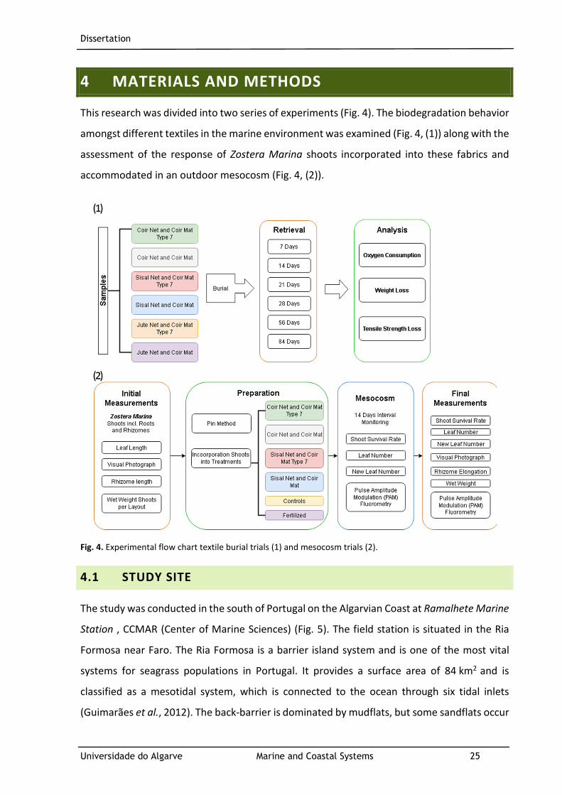
Dissertation
Universidade do Algarve Marine and Coastal Systems 25
4 MATERIALS AND METHODS
This research was divided into two series of experiments (Fig. 4). The biodegradation behavior
amongst different textiles in the marine environment was examined (Fig. 4, (1)) along with the
assessment of the response of Zostera Marina shoots incorporated into these fabrics and
accommodated in an outdoor mesocosm (Fig. 4, (2)).
Fig. 4. Experimental flow chart textile burial trials (1) and mesocosm trials (2).
4.1 STUDY SITE
The study was conducted in the south of Portugal on the Algarvian Coast at Ramalhete Marine
Station , CCMAR (Center of Marine Sciences) (Fig. 5). The field station is situated in the Ria
Formosa near Faro. The Ria Formosa is a barrier island system and is one of the most vital
systems for seagrass populations in Portugal. It provides a surface area of 84 km2 and is
classified as a mesotidal system, which is connected to the ocean through six tidal inlets
(Guimarães et al., 2012). The back-barrier is dominated by mudflats, but some sandflats occur
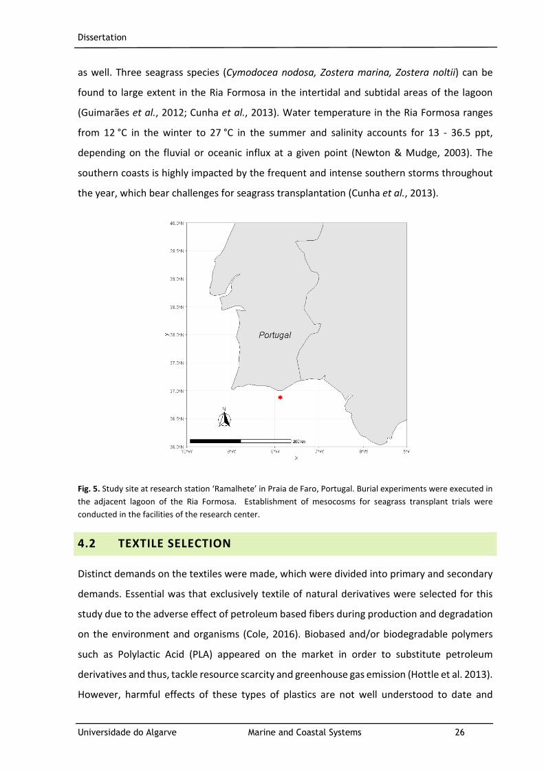
Dissertation
Universidade do Algarve Marine and Coastal Systems 26
as well. Three seagrass species (Cymodocea nodosa, Zostera marina, Zostera noltii) can be
found to large extent in the Ria Formosa in the intertidal and subtidal areas of the lagoon
(Guimarães et al., 2012; Cunha et al., 2013). Water temperature in the Ria Formosa ranges
from 12 °C in the winter to 27 °C in the summer and salinity accounts for 13 - 36.5 ppt,
depending on the fluvial or oceanic influx at a given point (Newton & Mudge, 2003). The
southern coasts is highly impacted by the frequent and intense southern storms throughout
the year, which bear challenges for seagrass transplantation (Cunha et al., 2013).
Fig. 5. Study site at research station ‘Ramalhete’ in Praia de Faro, Portugal. Burial experiments were executed in
the adjacent lagoon of the Ria Formosa. Establishment of mesocosms for seagrass transplant trials were
conducted in the facilities of the research center.
4.2 TEXTILE SELECTION
Distinct demands on the textiles were made, which were divided into primary and secondary
demands. Essential was that exclusively textile of natural derivatives were selected for this
study due to the adverse effect of petroleum based fibers during production and degradation
on the environment and organisms (Cole, 2016). Biobased and/or biodegradable polymers
such as Polylactic Acid (PLA) appeared on the market in order to substitute petroleum
derivatives and thus, tackle resource scarcity and greenhouse gas emission (Hottle et al. 2013).
However, harmful effects of these types of plastics are not well understood to date and
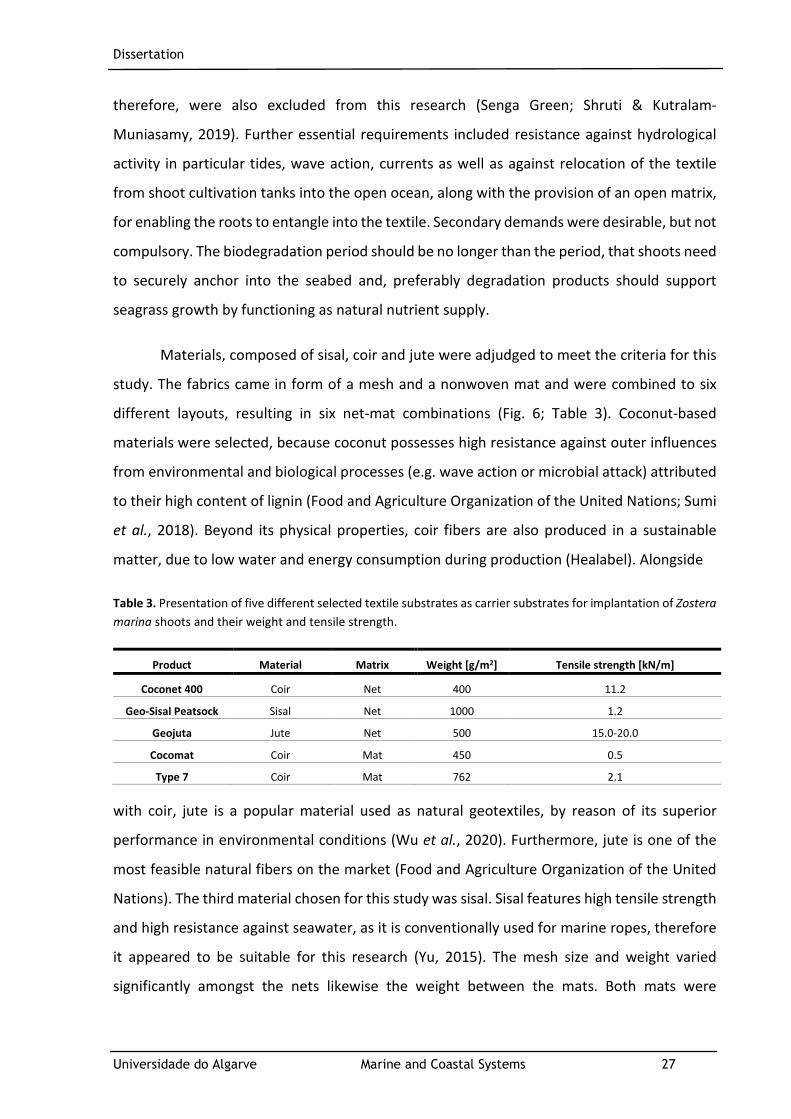
Dissertation
Universidade do Algarve Marine and Coastal Systems 27
therefore, were also excluded from this research (Senga Green; Shruti & Kutralam-
Muniasamy, 2019). Further essential requirements included resistance against hydrological
activity in particular tides, wave action, currents as well as against relocation of the textile
from shoot cultivation tanks into the open ocean, along with the provision of an open matrix,
for enabling the roots to entangle into the textile. Secondary demands were desirable, but not
compulsory. The biodegradation period should be no longer than the period, that shoots need
to securely anchor into the seabed and, preferably degradation products should support
seagrass growth by functioning as natural nutrient supply.
Materials, composed of sisal, coir and jute were adjudged to meet the criteria for this
study. The fabrics came in form of a mesh and a nonwoven mat and were combined to six
different layouts, resulting in six net-mat combinations (Fig. 6; Table 3). Coconut-based
materials were selected, because coconut possesses high resistance against outer influences
from environmental and biological processes (e.g. wave action or microbial attack) attributed
to their high content of lignin (Food and Agriculture Organization of the United Nations; Sumi
et al., 2018). Beyond its physical properties, coir fibers are also produced in a sustainable
matter, due to low water and energy consumption during production (Healabel). Alongside
Table 3. Presentation of five different selected textile substrates as carrier substrates for implantation of Zostera
marina shoots and their weight and tensile strength.
Product Material Matrix Weight [g/m2] Tensile strength [kN/m]
Coconet 400 Coir Net 400 11.2
Geo-Sisal Peatsock Sisal Net 1000 1.2
Geojuta Jute Net 500 15.0-20.0
Cocomat Coir Mat 450 0.5
Type 7 Coir Mat 762 2.1
with coir, jute is a popular material used as natural geotextiles, by reason of its superior
performance in environmental conditions (Wu et al., 2020). Furthermore, jute is one of the
most feasible natural fibers on the market (Food and Agriculture Organization of the United
Nations). The third material chosen for this study was sisal. Sisal features high tensile strength
and high resistance against seawater, as it is conventionally used for marine ropes, therefore
it appeared to be suitable for this research (Yu, 2015). The mesh size and weight varied
significantly amongst the nets likewise the weight between the mats. Both mats were

Dissertation
Universidade do Algarve Marine and Coastal Systems 28
composed of a coconut nonwoven, held together by a polypropylene net and thread, which
were removed before the beginning of the trials.
Fig. 6. Illustration of the substrate selection. Each mesh was combined with a mat, resulting in six different
layout designs. The mat was placed in between two layers of the mesh and the three layouers were sewn
together with a sisal thread, creating a so-called sandwich structure.
The textiles were coupled in six different combinations. Each mat was incorporated
into one net on the top and bottom and sewn together with a sisal thread, resulting in a so-
called sandwich structure (net-mat-net layout). The specimen measured 50 x 300 mm, the
standardized sample size for determining the maximum force at break (ISO 13934-1:1999).
Up to present, the performance and degradation rate of natural textiles placed in the
marine environment lacks knowledge and, data is primarily available on terrestrial
degradation processes. The following presented data on terrestrial biodegradation is based
on a comprehensive review of published peer-reviewed academic papers (Table 4) (Daria et
al., 2020).
Table 4. Terrestrial degradation behavior of natural materials. Data based on a comprehensive review of
several studies. Hence, the individual methodologies on testing the degradation behavior vary and therefore,
degradation time varies strongly. (Daria et al., 2020)
Material Time Interval [months]
Coconut 6-36
Jute 6-18
Sisal 12
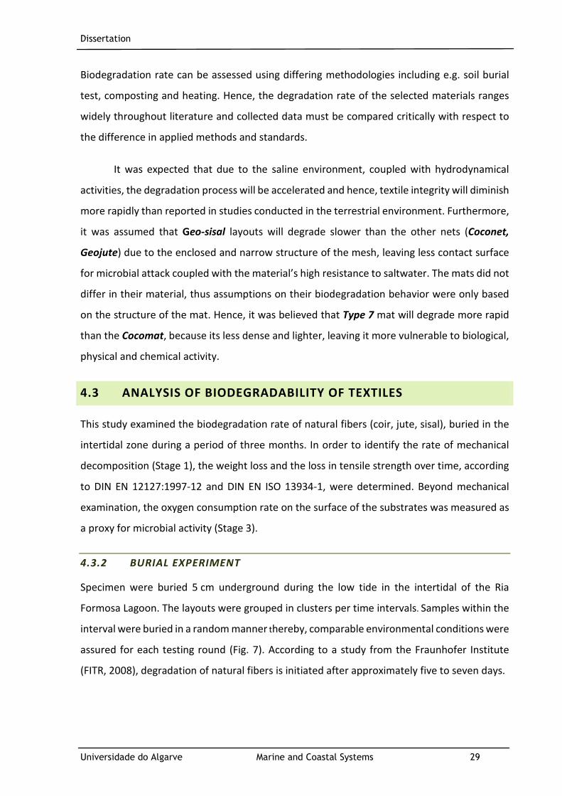
Dissertation
Universidade do Algarve Marine and Coastal Systems 29
Biodegradation rate can be assessed using differing methodologies including e.g. soil burial
test, composting and heating. Hence, the degradation rate of the selected materials ranges
widely throughout literature and collected data must be compared critically with respect to
the difference in applied methods and standards.
It was expected that due to the saline environment, coupled with hydrodynamical
activities, the degradation process will be accelerated and hence, textile integrity will diminish
more rapidly than reported in studies conducted in the terrestrial environment. Furthermore,
it was assumed that Geo-sisal layouts will degrade slower than the other nets (Coconet,
Geojute) due to the enclosed and narrow structure of the mesh, leaving less contact surface
for microbial attack coupled with the material’s high resistance to saltwater. The mats did not
differ in their material, thus assumptions on their biodegradation behavior were only based
on the structure of the mat. Hence, it was believed that Type 7 mat will degrade more rapid
than the Cocomat, because its less dense and lighter, leaving it more vulnerable to biological,
physical and chemical activity.
4.3 ANALYSIS OF BIODEGRADABILITY OF TEXTILES
This study examined the biodegradation rate of natural fibers (coir, jute, sisal), buried in the
intertidal zone during a period of three months. In order to identify the rate of mechanical
decomposition (Stage 1), the weight loss and the loss in tensile strength over time, according
to DIN EN 12127:1997-12 and DIN EN ISO 13934-1, were determined. Beyond mechanical
examination, the oxygen consumption rate on the surface of the substrates was measured as
a proxy for microbial activity (Stage 3).
4.3.2 BURIAL EXPERIMENT
Specimen were buried 5 cm underground during the low tide in the intertidal of the Ria
Formosa Lagoon. The layouts were grouped in clusters per time intervals. Samples within the
interval were buried in a random manner thereby, comparable environmental conditions were
assured for each testing round (Fig. 7). According to a study from the Fraunhofer Institute
(FITR, 2008), degradation of natural fibers is initiated after approximately five to seven days.
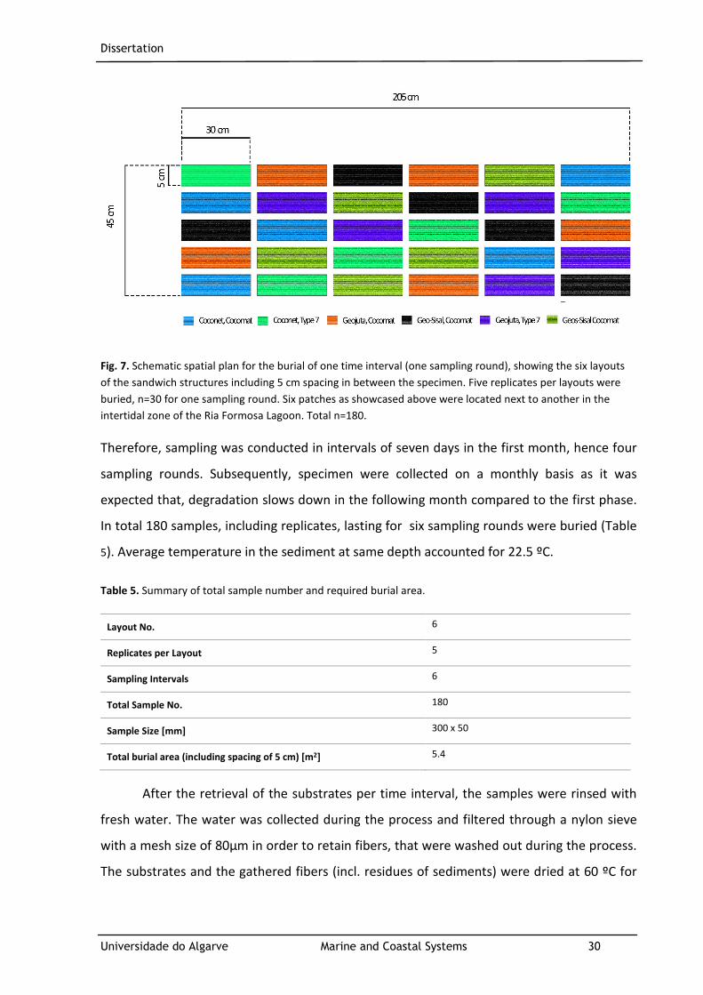
Dissertation
Universidade do Algarve Marine and Coastal Systems 30
Fig. 7. Schematic spatial plan for the burial of one time interval (one sampling round), showing the six layouts
of the sandwich structures including 5 cm spacing in between the specimen. Five replicates per layouts were
buried, n=30 for one sampling round. Six patches as showcased above were located next to another in the
intertidal zone of the Ria Formosa Lagoon. Total n=180.
Therefore, sampling was conducted in intervals of seven days in the first month, hence four
sampling rounds. Subsequently, specimen were collected on a monthly basis as it was
expected that, degradation slows down in the following month compared to the first phase.
In total 180 samples, including replicates, lasting for six sampling rounds were buried (Table
5). Average temperature in the sediment at same depth accounted for 22.5 ºC.
Table 5. Summary of total sample number and required burial area.
After the retrieval of the substrates per time interval, the samples were rinsed with
fresh water. The water was collected during the process and filtered through a nylon sieve
with a mesh size of 80µm in order to retain fibers, that were washed out during the process.
The substrates and the gathered fibers (incl. residues of sediments) were dried at 60 ºC for
Layout No. 6
Replicates per Layout 5
Sampling Intervals 6
Total Sample No. 180
Sample Size [mm] 300 x 50
Total burial area (including spacing of 5 cm) [m2] 5.4
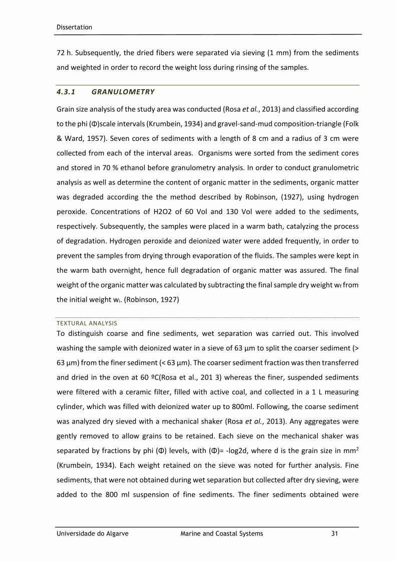
Dissertation
Universidade do Algarve Marine and Coastal Systems 31
72 h. Subsequently, the dried fibers were separated via sieving (1 mm) from the sediments
and weighted in order to record the weight loss during rinsing of the samples.
4.3.1 GRANULOMETRY
Grain size analysis of the study area was conducted (Rosa et al., 2013) and classified according
to the phi (Φ)scale intervals (Krumbein, 1934) and gravel-sand-mud composition-triangle (Folk
& Ward, 1957). Seven cores of sediments with a length of 8 cm and a radius of 3 cm were
collected from each of the interval areas. Organisms were sorted from the sediment cores
and stored in 70 % ethanol before granulometry analysis. In order to conduct granulometric
analysis as well as determine the content of organic matter in the sediments, organic matter
was degraded according the the method described by Robinson, (1927), using hydrogen
peroxide. Concentrations of H2O2 of 60 Vol and 130 Vol were added to the sediments,
respectively. Subsequently, the samples were placed in a warm bath, catalyzing the process
of degradation. Hydrogen peroxide and deionized water were added frequently, in order to
prevent the samples from drying through evaporation of the fluids. The samples were kept in
the warm bath overnight, hence full degradation of organic matter was assured. The final
weight of the organic matter was calculated by subtracting the final sample dry weight wf from
the initial weight wi. (Robinson, 1927)
TEXTURAL ANALYSIS
To distinguish coarse and fine sediments, wet separation was carried out. This involved
washing the sample with deionized water in a sieve of 63 μm to split the coarser sediment (>
63 μm) from the finer sediment (< 63 μm). The coarser sediment fraction was then transferred
and dried in the oven at 60 ºC(Rosa et al., 201 3) whereas the finer, suspended sediments
were filtered with a ceramic filter, filled with active coal, and collected in a 1 L measuring
cylinder, which was filled with deionized water up to 800ml. Following, the coarse sediment
was analyzed dry sieved with a mechanical shaker (Rosa et al., 2013). Any aggregates were
gently removed to allow grains to be retained. Each sieve on the mechanical shaker was
separated by fractions by phi (Φ) levels, with (Φ)= -log2d, where d is the grain size in mm2
(Krumbein, 1934). Each weight retained on the sieve was noted for further analysis. Fine
sediments, that were not obtained during wet separation but collected after dry sieving, were
added to the 800 ml suspension of fine sediments. The finer sediments obtained were
Dissertation
Universidade do Algarve Marine and Coastal Systems 32
analyzed by using the pipette method (Rosa et al., 2013). 70 ml of Sodium
Hexametaphosphate (3.04g/L) were added to the suspension and the samples homogenized
by mixing them with a rubber rod for two minutes and then letting them rest overnight.
Temperature was recorded before the analysis, on which the depth at which samples were
taken was based on. At the defined depth, a small portion of the suspension was taken from
the measuring cylinder using a graduated pipette at an increment of 20ml. Six withdrawals
per sample were collected in prior defined time intervals (Appendix 2). The withdrawals were
dried, and the weights taken and the associated scale phi (Φ) value intervals were calculated
(Krumbein, 1934)
GRANULOMETRIC PARAMETERS
A grain size distribution and statistics program, GRADISTAT was used to calculate
granulometric parameters, which runs within a Microsoft excel spreadsheet package (Blott &
Pye, 2001). Method of Moments was calculated in this program arithmetically (metric units),
geometrically and logarithmically (phi units) and using graphical moment of Folk & Ward,
(1957), allowing Folk and Ward descriptive terms to be applied to moments statistics (Blott &
Pye, 2001).
4.3.3 RELATIVE WEIGHT LOSS
In order to determine the relative weight loss over time, the initial weight wi of each specimen,
dried in the oven for 24 h at 60 ºC, was taken before the burial experiments. The final weight
wf of the retrieved samples was taken and the relative weight loss calculated in percentage
from the arithmetic means of wi and wf for each layout (adapted from Chakraborty et al.,
(2014)). The average weight of the retained fibers during washing ww was added to the final
weight in order to not falsely attribute it to the degradation process;
��������
���� 1
wi Initial weight
wf Final weight
ww
Weight rinsed out fibers
Dissertation
Universidade do Algarve Marine and Coastal Systems 33
4.3.4 TENSILE STRENGTHS LOSS
Tensile strength loss over time of the textiles was used as a descriptor for biodegradation as
well as for the evaluation of their suitability for this research. The carrier substrates must
feature sufficient tensile strength, when relocated from the mesocosm into the coastal
environment as well as resisting hydrodynamical forces, hence the slower the decline in
mechanical properties, the better. Examination of maximum force was conducted according
to the DIN EN ISO 13934-1 (Table 6) (ISO 13934-1:1999),executed on the INSTRON 5565.
Before testing, the sisal thread of the prior sewing process was removed.
Table 6. Parameters for tensile strength test procedures for textiles according to DIN EN ISO 13934-1 (ISO
13934-1:1999).
Specimen number Width [mm] Length [mm] Rate of Extension [mm/min] Pretension [N]
5 50 ± 0.5 200 + Clamps 100 0.5
Along with the samples, five controls were tested. Thereby, providing a set of data for
comparison, indicating the initial maximum force tsi of each layout prior burial. The arithmetic
mean was calculated for all layouts and controls and the relative tensile strength loss over
time computed;
�� ��������������
��������� 2
tsi Initial tensile strength
tsf Final tensile strength
4.3.5 AEROBIC BIODEGRADATION
As a proxy for the aerobic microbial biodegradation (Stage 3) oxygen levels were measured on
the surface of the textiles and converted into oxygen consumption rate (OCR) by fitting a linear
regression of the decreasing concentration and quantifying the negative slope in μmol
m−3min−1 (Dietz et al., 2019). A higher abundancy of organisms results in an increased oxygen
consumption rate, therefore it was expected, that the oxygen consumption rate will increase
throughout the experiment. Field luminescent DO sensors of the Hach OxygenHQ40D Portable
Dissolved Oxygen Meter were placed on top of the textile directly after retrieval.
Measurements were taken every 30 s for 5 mins.
Dissertation
Universidade do Algarve Marine and Coastal Systems 34
The oxygen optodes are composed of an oxygen sensitive membrane and measure the
oxygen in an optical manner. A manufacturer explains (Häck, 2003) how a sensing foil is
excited by a modulated blue light and, red light is emitted. The intensity of the emitted red
light expresses the amount of oxygen in the sample. As a control, a reference red LED is
emitted at the same time, without exiting the foil. (Häck, 2003) Controls, layouts prior burial,
were tested additionally. It was believed that the oxygen levels stay rather constant due to
the absence of aqueous aerobic microorganisms in the controls.
4.4 ANALYSIS OF ZOSTERA MARINA RESPONSE TO TEXTILES
4.4.1 SHOOT COLLECTION
A total number of 150 shoots of Zostera marina including roots, rhizomes and leaves were
harvested from donor meadows in the coastal lagoon Ria Formosa, on Culatra Island with the
required license. Plants were collected during low tide, ensuring easy accessibility. The shoots
were stored in outdoor tanks, at Ramalhete research center with incoming coarse-filtered
seawater at local temperature and salinity until preparation. According to Cunha et. al. (2009)
Culatra Island is a suitable donor site. However populations favor clonal production, resulting
in lower genetic diversity in the Ria Formosa meadows compared to central sites (Billingham
et al., 2003), which was found to limit transplantation success (Pazzaglia et al. 2021).
4.4.2 SHOOT PREPARATION
The shoots were digitally photographed next to a measuring tape and each leaf was measured
and its length (cm) recorded. Leaf elongation was obtained using the pin method according to
Short & Coles, (2001). A needle was poked through the leaf sheats allowing the growth
assessment at defined monitoring points (Fig. 8). The wet weight of five shoots was taken and
the shoots placed randomly into the textile with dimensions of 20 x 20 cm. Roots were pushed
through the top grid of the sandwich structure and placed on top of the nonwoven mat,
allowing the roots to interconnect with the mat (Fig. 9, left).

Dissertation
Universidade do Algarve Marine and Coastal Systems 35
Fig. 8. Pin method for marking seagrass in order obtain leaf elongation over time (Short & Coles, 2001).
A plan of the shoot location in each textile was drawn in order to identify the individual shoots
after the experiments and to draw a visual and morphological comparison of the shoot
development (Fig. 9, right).
Fig. 9. Left: Shoot incorporation into sandwich structure. Shoot incl. rhizomes and roots was placed through the
mesh but kept on top of the mat. Right: Example of schematic plan of shoot localization within textile. Green
dots represent the shoots and the orange tag identifies the textile layout and replica number.
Five replicas of each textile layout were prepared. The jute net was excluded from this
experiment due to its poor performance in the biodegradation trials, therefore a total number
of 20 mesocosms, accommodating textile + shoots, were prepared.
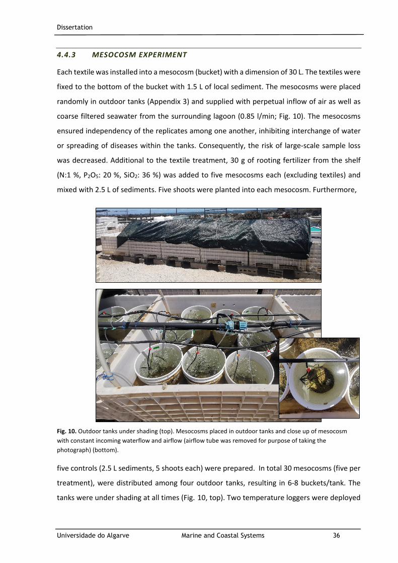
Dissertation
Universidade do Algarve Marine and Coastal Systems 36
4.4.3 MESOCOSM EXPERIMENT
Each textile was installed into a mesocosm (bucket) with a dimension of 30 L. The textiles were
fixed to the bottom of the bucket with 1.5 L of local sediment. The mesocosms were placed
randomly in outdoor tanks (Appendix 3) and supplied with perpetual inflow of air as well as
coarse filtered seawater from the surrounding lagoon (0.85 l/min; Fig. 10). The mesocosms
ensured independency of the replicates among one another, inhibiting interchange of water
or spreading of diseases within the tanks. Consequently, the risk of large-scale sample loss
was decreased. Additional to the textile treatment, 30 g of rooting fertilizer from the shelf
(N:1 %, P2O5: 20 %, SiO2: 36 %) was added to five mesocosms each (excluding textiles) and
mixed with 2.5 L of sediments. Five shoots were planted into each mesocosm. Furthermore,
Fig. 10. Outdoor tanks under shading (top). Mesocosms placed in outdoor tanks and close up of mesocosm
with constant incoming waterflow and airflow (airflow tube was removed for purpose of taking the
photograph) (bottom).
five controls (2.5 L sediments, 5 shoots each) were prepared. In total 30 mesocosms (five per
treatment), were distributed among four outdoor tanks, resulting in 6-8 buckets/tank. The
tanks were under shading at all times (Fig. 10, top). Two temperature loggers were deployed
Dissertation
Universidade do Algarve Marine and Coastal Systems 37
on the two outer sides of the tanks, alongside with two more loggers inside the buckets on
the outer edges of the tank. Additionally, two HOBO light intensity loggers were fixed to two
buckets on each outer edge of the tanks. Salinity, pH and dissolved oxygen data was supplied
from the Ramalhete field station.
4.4.4 EXAMINATION OF SEAGRASS RESPONSE TO TEXTILE
The shoots were monitored in biweekly time intervals for seven weeks and assessed on their
i. Shoot survival rate (number shoots/ mesocosm)
ii. Leaf number per shoot
iii. Number of new leaves per mesocosm
iv. Leaf elongation per mesocosm – aborted due to failure of monitoring
v. Total root segment elongation per mesocosm
vi. Pulse-Amplitude-Modulation (PAM): Effective yield of three shoots per
mesocosm
The shoots were removed from the textiles after seven weeks and final measurements were
taken along with digital photographs of each shoot.
Each new leaf that appeared was marked and counted. Total number of new
developed leaves over the course of the experiment was recorded per treatment.
Root segments were measured from the digital photographs in the program ImageJ
and summed up to a total length per mesocosm. Same measurements were taken at the end
of the experiment and the relative rhizome elongation or loss were computed.
In order to identify the stabilization effect of the carrier textile on the shoots, the root
entanglement into the textile was inspected at the end of the experiment.
4.4.5 PULSE-AMPLITUDE-MODULATION (PAM)
The transformation of light energy into chemically fixed energy gives origin to chlorophyll (Chi)
a fluorescence, which channels the absorbed light into the reaction centers photosystems I
(PSI) and II (PSII) of an organism, where photochemical energy conversion and heat dissipation
happens (Wageningen University & Research, n.a.; Papageorgiou & Govindjee, op. 2010).
Dissertation
Universidade do Algarve Marine and Coastal Systems 38
Therefore, determination of Chlorophyll (Chi) a fluorescence has been used widely as estimate
for photosynthesis (Papageorgiou & Govindjee, op. 2010). The PSII is mainly responsible for
fluctuation in fluorescence and, thereby indicates variations in PSII photochemical efficiency
and heat dissipation (Wageningen University & Research, n.a.).
Pulse-Amplitude-Modulation (PAM), a combination of fluorometry and the saturation
pulse method, has been one of the most powerful in situ and in vivo technique in quantifying
photosynthetic productivity (Wageningen University & Research, n.a.; Papageorgiou &
Govindjee, op. 2010; Pavlovic et al., 2014). The Fv/Fm ([(Fm -F0)/Fm]) ratio, which derives from
the minimal fluorescence yield (F0) and the maximum yield (Fm), after superimposing a light
beam onto the prior dark-adapted leaf, indicates the maximum photochemical efficiency of
the PSII and is proportional to the effective yield of photochemistry (Guidi et al., 2019).
The effect of the different treatments on the integrity of the seagrasses was assessed
by measuring the quantum effective yield Y of three representative shoots per replicate every
two weeks using a Walz DIVING-PAM (Pavlovic et al., 2014; Appendix 11). Prior
measurements, a section of each leaf, 2 cm above the sheath, was darkened with a non-
destructive clip (6.5 g), that possesses a small shutter, preventing light from entering. The
shutter was reopened after five minutes and the fiberoptic positioned on the leaf (Heinz Walz
GmbH, 1998). The Dark Clip allows a precise placement of the fiberoptics on the sample. The
fiberoptics were positioned in a 90º angle with regard to the leaf surface and were kept at a
distance of 3 mm (Heinz Walz GmbH, 1998). Background signals were compensated through
the AUTO-ZERO command, which was initially performed (Heinz Walz GmbH, 1998).
4.5 STATISTICAL ANALYSES
For all analyses the significance level α = 0.05 was defined. Outliers were removed and
substituted with the median. Subsequently, the data was logarithmized and normalized in
PRIMER 6. Normality test and trend detection were conducted with the programming
language R Commander 4.1.0. Despite the normalization of the data, the Sharpio-Wilk test
detected a non-normal distribution (Appendix 5), therefore non-parametric methods were
applied to the data.

Dissertation
Universidade do Algarve Marine and Coastal Systems 39
PERMANOVA analysis was executed in PRIMER 6 in order to detect differences among
textiles along with PERMADISP analysis in case of increased variance within a parameter. The
analysis was applied for burial as well as mesocosm experiments.
Boxplots and line graphs were generated in the program Matlab. Boxplot charts were
generated from five replicates per layout and time interval for burial and mesocosm
experiments. Values for the line graphs of the mesocosm experiment were computed from
the median of the concerned parameter per layout and monitoring point, always consisting of
five replicates together with the standard deviation.
Statistical hypothesis tested:
H0: Growth and integrity of Zostera marina shoots does not perform differently by the
fixation of the shoots into a carrier substrate than single shoots out planted directly into the
sediment.

Dissertation
Universidade do Algarve Marine and Coastal Systems 40
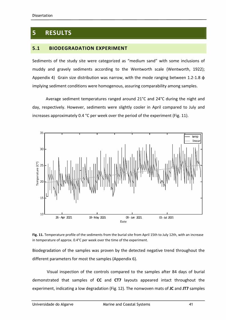
Dissertation
Universidade do Algarve Marine and Coastal Systems 41
5 RESULTS
5.1 BIODEGRADATION EXPERIMENT
Sediments of the study site were categorized as “medium sand” with some inclusions of
muddy and gravely sediments according to the Wentworth scale (Wentworth, 1922);
Appendix 4) Grain size distribution was narrow, with the mode ranging between 1.2-1.8 φ
implying sediment conditions were homogenous, assuring comparability among samples.
Average sediment temperatures ranged around 21°C and 24°C during the night and
day, respectively. However, sediments were slightly cooler in April compared to July and
increases approximately 0.4 °C per week over the period of the experiment (Fig. 11).
Fig. 11. Temperature profile of the sediments from the burial site from April 15th to July 12th, with an increase
in temperature of approx. 0.4°C per week over the time of the experiment.
Biodegradation of the samples was proven by the detected negative trend throughout the
different parameters for most the samples (Appendix 6).
Visual inspection of the controls compared to the samples after 84 days of burial
demonstrated that samples of CC and CT7 layouts appeared intact throughout the
experiment, indicating a low degradation (Fig. 12). The nonwoven mats of JC and JT7 samples
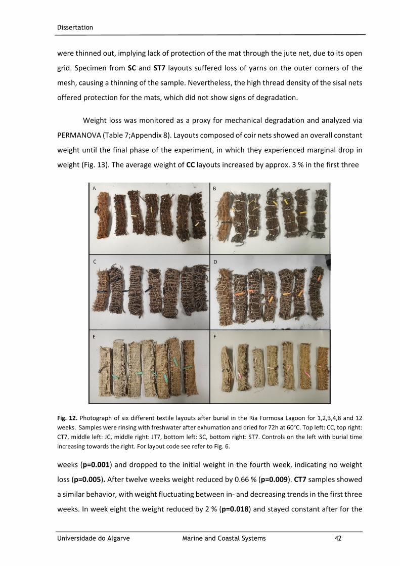
Dissertation
Universidade do Algarve Marine and Coastal Systems 42
were thinned out, implying lack of protection of the mat through the jute net, due to its open
grid. Specimen from SC and ST7 layouts suffered loss of yarns on the outer corners of the
mesh, causing a thinning of the sample. Nevertheless, the high thread density of the sisal nets
offered protection for the mats, which did not show signs of degradation.
Weight loss was monitored as a proxy for mechanical degradation and analyzed via
PERMANOVA (Table 7;Appendix 8). Layouts composed of coir nets showed an overall constant
weight until the final phase of the experiment, in which they experienced marginal drop in
weight (Fig. 13). The average weight of CC layouts increased by approx. 3 % in the first three
Fig. 12. Photograph of six different textile layouts after burial in the Ria Formosa Lagoon for 1,2,3,4,8 and 12
weeks. Samples were rinsing with freshwater after exhumation and dried for 72h at 60°C. Top left: CC, top right:
CT7, middle left: JC, middle right: JT7, bottom left: SC, bottom right: ST7. Controls on the left with burial time
increasing towards the right. For layout code see refer to Fig. 6.
weeks (p=0.001) and dropped to the initial weight in the fourth week, indicating no weight
loss (p=0.005). After twelve weeks weight reduced by 0.66 % (p=0.009). CT7 samples showed
a similar behavior, with weight fluctuating between in- and decreasing trends in the first three
weeks. In week eight the weight reduced by 2 % (p=0.018) and stayed constant after for the

Dissertation
Universidade do Algarve Marine and Coastal Systems 43
following month (p=0.393). No weight loss was recorded for the JC layout within the first four
weeks but a sudden drop was recorded after eight weeks with a final weight loss of 15 %
(p=0.002). JT7 replicates varied among each other within the first four weeks, indicated by the
high variance in week three and four, though lowered overall 7 % after eight weeks, which
Fig. 13. Relative weight loss of buried textile layouts over time starting after week 1 until week 12. Each boxplot
represents five replicates per time interval. Letters below boxplot charts explain differences within individual
layouts over time. Letters in the box below boxplot charts explain difference in one time interval among the
layouts.
was doubled after twelve weeks (p=0.001). Weight of SC textiles reduced in the first week of
burial by 7 % (p=0.001) and stayed constant for the following three weeks until it dropped by
14 % and 21 % in week eight and twelve, respectively (p≤0.013). The same pattern of weight
loss was observed for ST7 samples, which lost in total 18 % of their initial weight (p=0.001).
Among layouts, samples composed from coir nets showed the lowest weight loss, opposed to
the 30x and 10x higher weight loss of sisal net layouts for CC and CT7, respectively (p=0.001)
(Fig. 17, top). Final weight loss of jute net layouts ranged in between coconut (avg. 10x higher)
and sisal layouts (avg. 1.5 x lower) (p≤0.017). No differentiation between the mats within one
group of nets could be made.
The second indicator examined for mechanical degradation was tensile strength loss
(Fig. 14;Appendix 7). Tensile strength loss of CC layouts did not show differences up to three
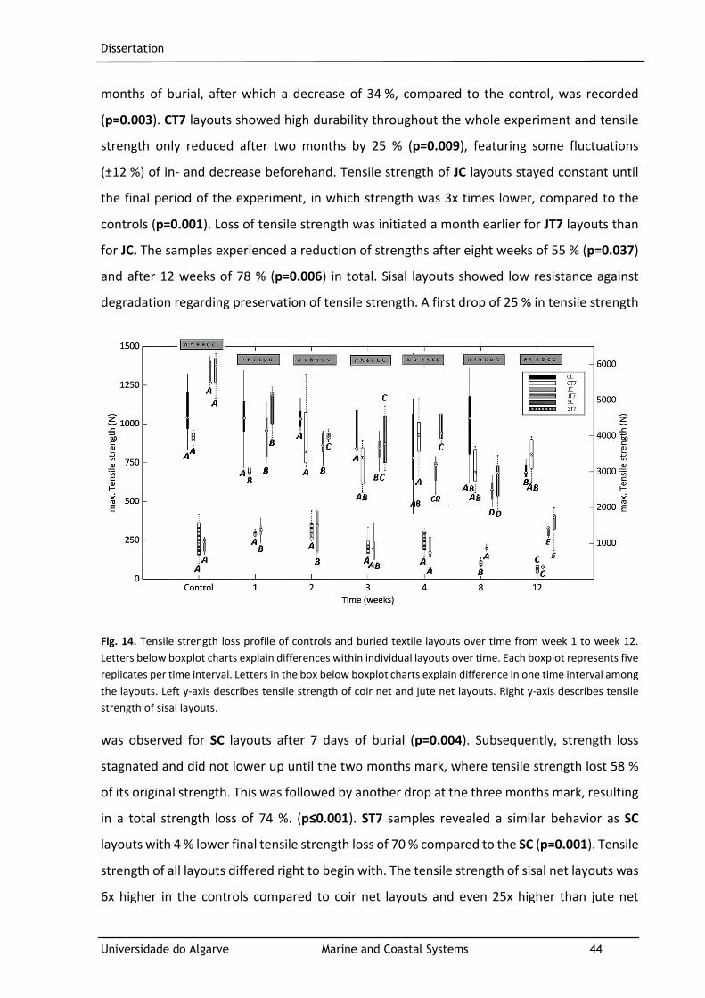
Dissertation
Universidade do Algarve Marine and Coastal Systems 44
months of burial, after which a decrease of 34 %, compared to the control, was recorded
(p=0.003). CT7 layouts showed high durability throughout the whole experiment and tensile
strength only reduced after two months by 25 % (p=0.009), featuring some fluctuations
(±12 %) of in- and decrease beforehand. Tensile strength of JC layouts stayed constant until
the final period of the experiment, in which strength was 3x times lower, compared to the
controls (p=0.001). Loss of tensile strength was initiated a month earlier for JT7 layouts than
for JC. The samples experienced a reduction of strengths after eight weeks of 55 % (p=0.037)
and after 12 weeks of 78 % (p=0.006) in total. Sisal layouts showed low resistance against
degradation regarding preservation of tensile strength. A first drop of 25 % in tensile strength
Fig. 14. Tensile strength loss profile of controls and buried textile layouts over time from week 1 to week 12.
Letters below boxplot charts explain differences within individual layouts over time. Each boxplot represents five
replicates per time interval. Letters in the box below boxplot charts explain difference in one time interval among
the layouts. Left y-axis describes tensile strength of coir net and jute net layouts. Right y-axis describes tensile
strength of sisal layouts.
was observed for SC layouts after 7 days of burial (p=0.004). Subsequently, strength loss
stagnated and did not lower up until the two months mark, where tensile strength lost 58 %
of its original strength. This was followed by another drop at the three months mark, resulting
in a total strength loss of 74 %. (p≤0.001). ST7 samples revealed a similar behavior as SC
layouts with 4 % lower final tensile strength loss of 70 % compared to the SC (p=0.001). Tensile
strength of all layouts differed right to begin with. The tensile strength of sisal net layouts was
6x higher in the controls compared to coir net layouts and even 25x higher than jute net
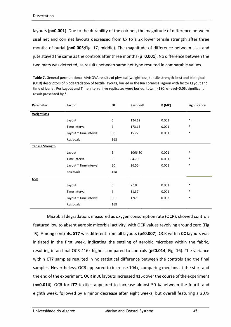
Dissertation
Universidade do Algarve Marine and Coastal Systems 45
layouts (p=0.001). Due to the durability of the coir net, the magnitude of difference between
sisal net and coir net layouts decreased from 6x to a 2x lower tensile strength after three
months of burial (p=0.005;Fig. 17, middle). The magnitude of difference between sisal and
jute stayed the same as the controls after three months (p=0.001). No difference between the
two mats was detected, as results between same net type resulted in comparable values.
Table 7. General permutational MANOVA results of physical (weight loss, tensile strength loss) and biological
(OCR) descriptors of biodegradation of textile layouts, buried in the Ria Formosa lagoon with factor Layout and
time of burial. Per Layout and Time interval five replicates were buried, total n=180. α-level=0.05, significant
result presented by *.
Parameter Factor DF Pseudo-F P (MC) Significance
Weight loss
Layout 5 124.12 0.001 *
Time interval 6 173.13 0.001 *
Layout * Time interval 30 15.22 0.001 *
Residuals 168
Tensile Strength
Layout 5 1066.80 0.001 *
Time interval 6 84.79 0.001 *
Layout * Time interval 30 26.55 0.001 *
Residuals 168
OCR
Layout 5 7.10 0.001 *
Time interval 6 11.37 0.001 *
Layout * Time interval 30 1.97 0.002 *
Residuals 168
Microbial degradation, measured as oxygen consumption rate (OCR), showed controls
featured low to absent aerobic micorbial activity, with OCR values revolving around zero (Fig
15). Among controls, ST7 was different from all layouts (p≤0.007). OCR within CC layouts was
initiated in the first week, indicating the settling of aerobic microbes within the fabric,
resulting in an final OCR 416x higher compared to controls (p≤0.014; Fig. 16). The variance
within CT7 samples resulted in no statistical difference between the controls and the final
samples. Nevertheless, OCR appeared to increase 104x, comparing medians at the start and
the end of the experiment. OCR in JC layouts increased 415x over the course of the experiment
(p=0.014). OCR for JT7 textiles appeared to increase almost 50 % between the fourth and
eighth week, followed by a minor decrease after eight weeks, but overall featuring a 207x

Dissertation
Universidade do Algarve Marine and Coastal Systems 46
higher OCR at the final stage compared to the controls (p≤0.016). Differences of OCR for SC
layouts were recorded after two months, accounting for a 63x higher OCR than the controls
(p=0.018). Threshold for ST7 structures was observed after twelve weeks, featuring a 27x
higher OCR than at the start (p=0.006). Up until the second week OCR among layouts did not
indicate any distinction. After the third week some differentiation was noted in between sisal
net structures and JC as well as in between SC and CT7 layouts (p=<0.018), which however,
disappeared towards the end of the experiment. Although final values of OCR are only half as
high in CC layouts than in the other layouts (p≤0.04), the highest increase over time, in
comparison with the control, was recorded for this structure, followed by JC and JT7 layouts.
Similar pattern was observed for sisal net layouts. Despite comparable final values, SC
experienced a 2x higher increase of OCR than ST7 layouts, when comparing controls and final
rates. Variance increased on average 1400x from the controls to the final time point of three
months (p= 0.001), possibly influencing PERMANOVA results.
In conclusion coir net layouts sustained their morphological appearance along with
mechanical integrity the greatest throughout the experiment (Fig. 17). Yet, especially CC
layouts possessed a pronounced duplication of microbial respiration. Despite the increased
duplication, total OCR was rather low in coir net layouts. In contrast, sisal net layouts suffered
from instant weight and tensile strength loss as well as increased total microbial respiration,
regardless of the comparatively low duplication. Weight loss in jute net layouts was slightly
slower than in sisal net ones, however tensile strength loss appeared to be similar. Aerobic
activity was increased, comparable to the sisal net layouts.
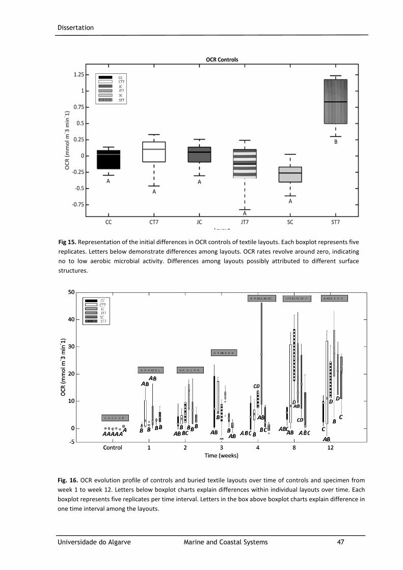
Dissertation
Universidade do Algarve Marine and Coastal Systems 47
Fig. 16. OCR evolution profile of controls and buried textile layouts over time of controls and specimen from
week 1 to week 12. Letters below boxplot charts explain differences within individual layouts over time. Each
boxplot represents five replicates per time interval. Letters in the box above boxplot charts explain difference in
one time interval among the layouts.
Fig 15. Representation of the initial differences in OCR controls of textile layouts. Each boxplot represents five
replicates. Letters below demonstrate differences among layouts. OCR rates revolve around zero, indicating
no to low aerobic microbial activity. Differences among layouts possibly attributed to different surface
structures.

Dissertation
Universidade do Algarve Marine and Coastal Systems 48
Fig. 17. Top: Relative weight loss of buried textile layouts after twelve weeks. Each boxplot represents five
replicates per time interval. Letters below boxplot charts indicate final differences among layouts. Middle:
Relative tensile strength loss of buried textile layouts after twelve weeks. Each boxplot represents five replicates
per time interval. Letters below boxplot charts indicate final differences among layouts. Bottom: Duplication of
microbial respiration (OCR) in textile layouts, comparing control rates with rates of layouts, retrieved after twelve
months. Each boxplot represents five replicates per time interval. Letters below boxplot charts indicate final
differences among layouts.
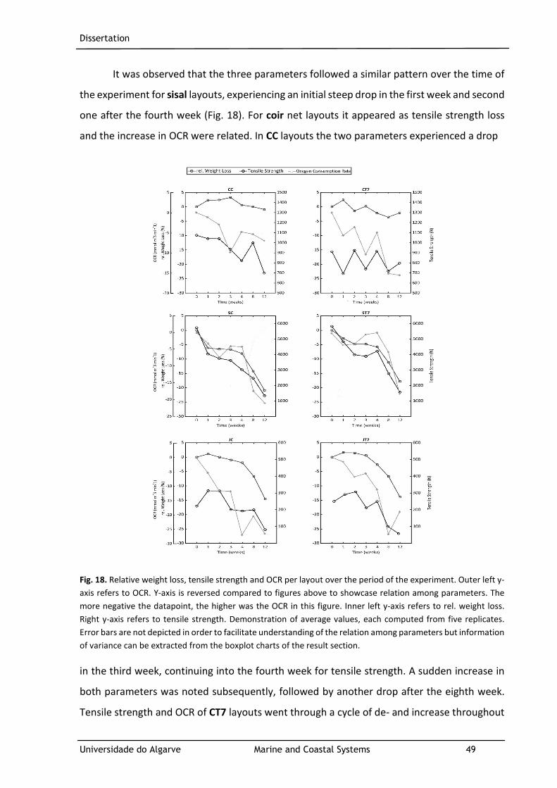
Dissertation
Universidade do Algarve Marine and Coastal Systems 49
It was observed that the three parameters followed a similar pattern over the time of
the experiment for sisal layouts, experiencing an initial steep drop in the first week and second
one after the fourth week (Fig. 18). For coir net layouts it appeared as tensile strength loss
and the increase in OCR were related. In CC layouts the two parameters experienced a drop
Fig. 18. Relative weight loss, tensile strength and OCR per layout over the period of the experiment. Outer left y-
axis refers to OCR. Y-axis is reversed compared to figures above to showcase relation among parameters. The
more negative the datapoint, the higher was the OCR in this figure. Inner left y-axis refers to rel. weight loss.
Right y-axis refers to tensile strength. Demonstration of average values, each computed from five replicates.
Error bars are not depicted in order to facilitate understanding of the relation among parameters but information
of variance can be extracted from the boxplot charts of the result section.
in the third week, continuing into the fourth week for tensile strength. A sudden increase in
both parameters was noted subsequently, followed by another drop after the eighth week.
Tensile strength and OCR of CT7 layouts went through a cycle of de- and increase throughout

Dissertation
Universidade do Algarve Marine and Coastal Systems 50
the experiment. The three descriptors of biodegradation showed no analogous behavior for
jute layouts. All parameters featured a terminal decrease but the fluctuations in between time
intervals were different among them.
5.2 MESOCOSM EXPERIMENT
Water temperature ranged between 19 °C and 28 °C (night/day) and was on average 24.5 °C
(σ = 1.19) from June to August (Fig. 19). No temperature difference between the two sides of
the tanks was observed (Appendix 9). Dissolved oxygen accounted for 94 % (σ = 0.16) and
showed an average difference of 2 % between June and August. The pH was 7.91 (σ = 0.16)
and stayed constant over the period of the experiment. Constant behavior was also observed
for salinity with an average of 37.4 psu (σ = 0.46).
Fig. 19. Physical parameters of the water pumped from the Ria Formosa Lagoon into Ramalhete research station.
Mesocosms were provided with this water and supplied with a constant water inflow at all times. Temperature
shown here is analogous to logged temperature in the tanks and buckets.
Daily light intensity on the northeast face of the tanks was on average 526.17 lux (σ = 401.06)
(Fig. 20). The southwest facing side showed a higher illuminance, accounting for 2316.13 lux
(σ = 2245.01).
Shoot integrity suffered severely over the course of the experiment (Fig. 21; Appendix
10). On average the relative leaf number decreased by 80 - 100 % in all treatments (p≤0.015)
after seven weeks (Fig. 22, top). No overall difference among the layouts was detected
(p=0.968). Yet, after one week CC layouts had 15 % and 20 % more leaves than SC layouts and
fertilized mesocosms, respectively (p≤0.019). Nevertheless, no distinction could be made
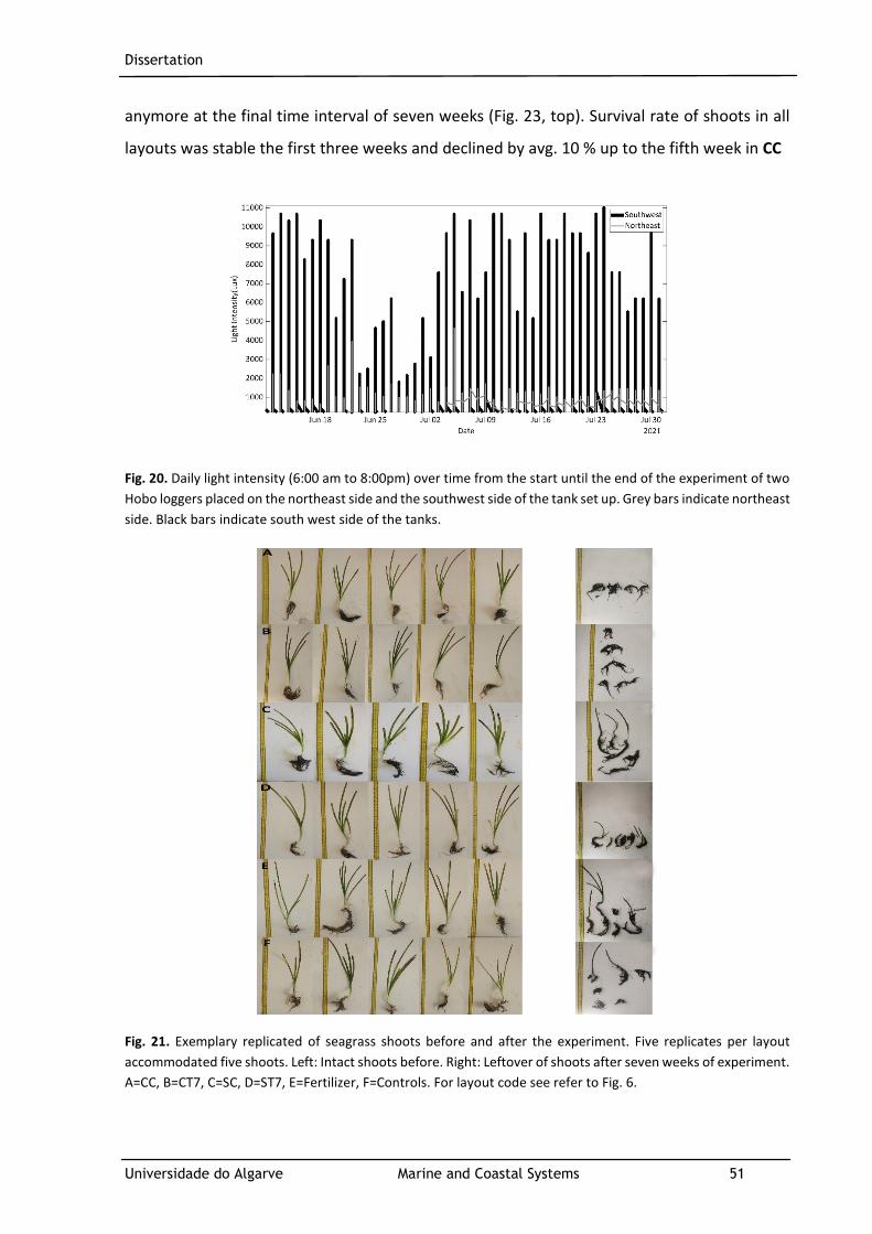
Dissertation
Universidade do Algarve Marine and Coastal Systems 51
anymore at the final time interval of seven weeks (Fig. 23, top). Survival rate of shoots in all
layouts was stable the first three weeks and declined by avg. 10 % up to the fifth week in CC
Fig. 20. Daily light intensity (6:00 am to 8:00pm) over time from the start until the end of the experiment of two
Hobo loggers placed on the northeast side and the southwest side of the tank set up. Grey bars indicate northeast
side. Black bars indicate south west side of the tanks.
Fig. 21. Exemplary replicated of seagrass shoots before and after the experiment. Five replicates per layout
accommodated five shoots. Left: Intact shoots before. Right: Leftover of shoots after seven weeks of experiment.
A=CC, B=CT7, C=SC, D=ST7, E=Fertilizer, F=Controls. For layout code see refer to Fig. 6.
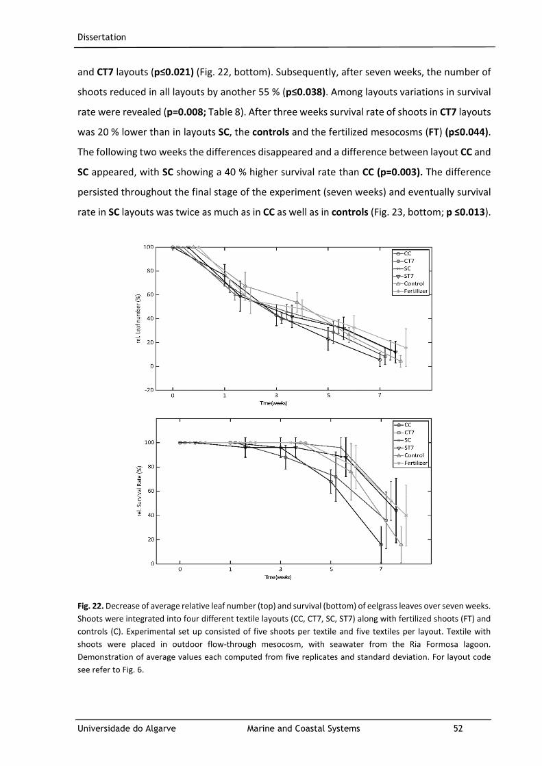
Dissertation
Universidade do Algarve Marine and Coastal Systems 52
and CT7 layouts (p≤0.021) (Fig. 22, bottom). Subsequently, after seven weeks, the number of
shoots reduced in all layouts by another 55 % (p≤0.038). Among layouts variations in survival
rate were revealed (p=0.008; Table 8). After three weeks survival rate of shoots in CT7 layouts
was 20 % lower than in layouts SC, the controls and the fertilized mesocosms (FT) (p≤0.044).
The following two weeks the differences disappeared and a difference between layout CC and
SC appeared, with SC showing a 40 % higher survival rate than CC (p=0.003). The difference
persisted throughout the final stage of the experiment (seven weeks) and eventually survival
rate in SC layouts was twice as much as in CC as well as in controls (Fig. 23, bottom; p ≤0.013).
Fig. 22. Decrease of average relative leaf number (top) and survival (bottom) of eelgrass leaves over seven weeks.
Shoots were integrated into four different textile layouts (CC, CT7, SC, ST7) along with fertilized shoots (FT) and
controls (C). Experimental set up consisted of five shoots per textile and five textiles per layout. Textile with
shoots were placed in outdoor flow-through mesocosm, with seawater from the Ria Formosa lagoon.
Demonstration of average values each computed from five replicates and standard deviation. For layout code
see refer to Fig. 6.
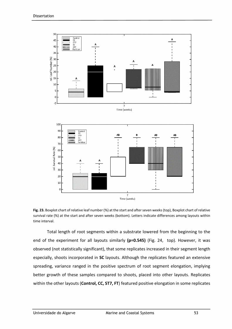
Dissertation
Universidade do Algarve Marine and Coastal Systems 53
Fig. 23. Boxplot chart of relative leaf number (%) at the start and after seven weeks (top), Boxplot chart of relative
survival rate (%) at the start and after seven weeks (bottom). Letters indicate differences among layouts within
time interval.
Total length of root segments within a substrate lowered from the beginning to the
end of the experiment for all layouts similarly (p=0.545) (Fig. 24, top). However, it was
observed (not statistically significant), that some replicates increased in their segment length
especially, shoots incorporated in SC layouts. Although the replicates featured an extensive
spreading, variance ranged in the positive spectrum of root segment elongation, implying
better growth of these samples compared to shoots, placed into other layouts. Replicates
within the other layouts (Control, CC, ST7, FT) featured positive elongation in some replicates
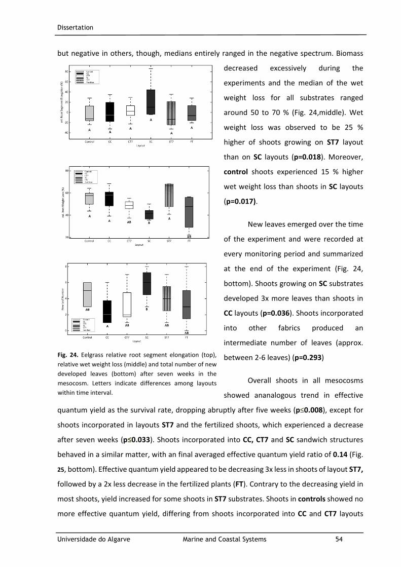
Dissertation
Universidade do Algarve Marine and Coastal Systems 54
but negative in others, though, medians entirely ranged in the negative spectrum. Biomass
decreased excessively during the
experiments and the median of the wet
weight loss for all substrates ranged
around 50 to 70 % (Fig. 24,middle). Wet
weight loss was observed to be 25 %
higher of shoots growing on ST7 layout
than on SC layouts (p=0.018). Moreover,
control shoots experienced 15 % higher
wet weight loss than shoots in SC layouts
(p=0.017).
New leaves emerged over the time
of the experiment and were recorded at
every monitoring period and summarized
at the end of the experiment (Fig. 24,
bottom). Shoots growing on SC substrates
developed 3x more leaves than shoots in
CC layouts (p=0.036). Shoots incorporated
into other fabrics produced an
intermediate number of leaves (approx.
between 2-6 leaves) (p=0.293)
Overall shoots in all mesocosms
showed ananalogous trend in effective
quantum yield as the survival rate, dropping abruptly after five weeks (p≤0.008), except for
shoots incorporated in layouts ST7 and the fertilized shoots, which experienced a decrease
after seven weeks (p≤0.033). Shoots incorporated into CC, CT7 and SC sandwich structures
behaved in a similar matter, with an final averaged effective quantum yield ratio of 0.14 (Fig.
25, bottom). Effective quantum yield appeared to be decreasing 3x less in shoots of layout ST7,
followed by a 2x less decrease in the fertilized plants (FT). Contrary to the decreasing yield in
most shoots, yield increased for some shoots in ST7 substrates. Shoots in controls showed no
more effective quantum yield, differing from shoots incorporated into CC and CT7 layouts
Fig. 24. Eelgrass relative root segment elongation (top),
relative wet weight loss (middle) and total number of new
developed leaves (bottom) after seven weeks in the
mesocosm. Letters indicate differences among layouts
within time interval.
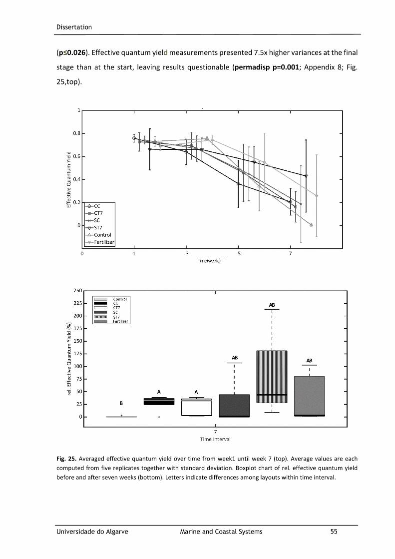
Dissertation
Universidade do Algarve Marine and Coastal Systems 55
(p≤0.026). Effective quantum yield measurements presented 7.5x higher variances at the final
stage than at the start, leaving results questionable (permadisp p=0.001; Appendix 8; Fig.
25,top).
Fig. 25. Averaged effective quantum yield over time from week1 until week 7 (top). Average values are each
computed from five replicates together with standard deviation. Boxplot chart of rel. effective quantum yield
before and after seven weeks (bottom). Letters indicate differences among layouts within time interval.
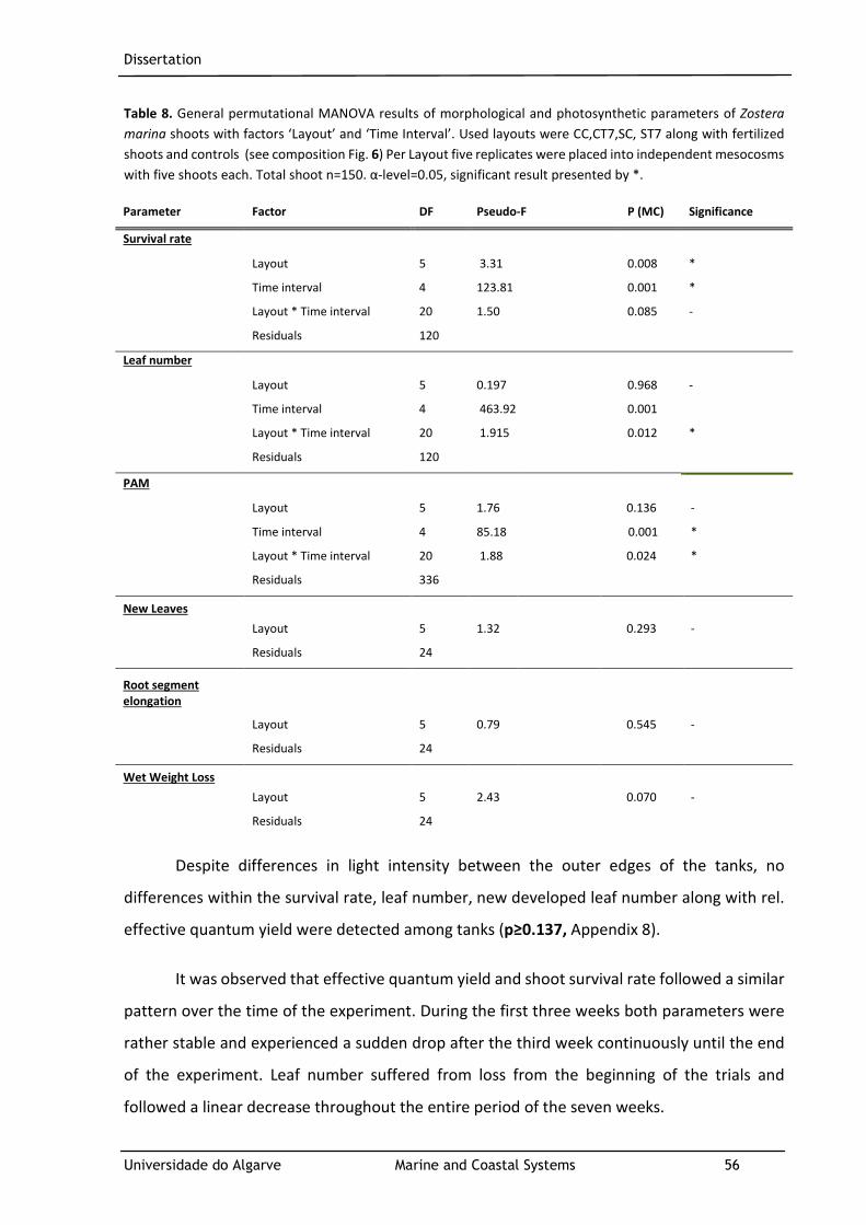
Dissertation
Universidade do Algarve Marine and Coastal Systems 56
Table 8. General permutational MANOVA results of morphological and photosynthetic parameters of Zostera
marina shoots with factors ‘Layout’ and ‘Time Interval’. Used layouts were CC,CT7,SC, ST7 along with fertilized
shoots and controls (see composition Fig. 6) Per Layout five replicates were placed into independent mesocosms
with five shoots each. Total shoot n=150. α-level=0.05, significant result presented by *.
Parameter Factor DF Pseudo-F P (MC) Significance
Survival rate
Layout 5 3.31 0.008 *
Time interval 4 123.81 0.001 *
Layout * Time interval 20 1.50 0.085 -
Residuals 120
Leaf number
Layout 5 0.197 0.968 -
Time interval 4 463.92 0.001
Layout * Time interval 20 1.915 0.012 *
Residuals 120
PAM
Layout 5 1.76 0.136 -
Time interval 4 85.18 0.001 *
Layout * Time interval 20 1.88 0.024 *
Residuals 336
New Leaves
Layout 5 1.32 0.293 -
Residuals 24
Root segment
elongation
Layout 5 0.79 0.545 -
Residuals 24
Wet Weight Loss
Layout 5 2.43 0.070 -
Residuals 24
Despite differences in light intensity between the outer edges of the tanks, no
differences within the survival rate, leaf number, new developed leaf number along with rel.
effective quantum yield were detected among tanks (p≥0.137, Appendix 8).
It was observed that effective quantum yield and shoot survival rate followed a similar
pattern over the time of the experiment. During the first three weeks both parameters were
rather stable and experienced a sudden drop after the third week continuously until the end
of the experiment. Leaf number suffered from loss from the beginning of the trials and
followed a linear decrease throughout the entire period of the seven weeks.
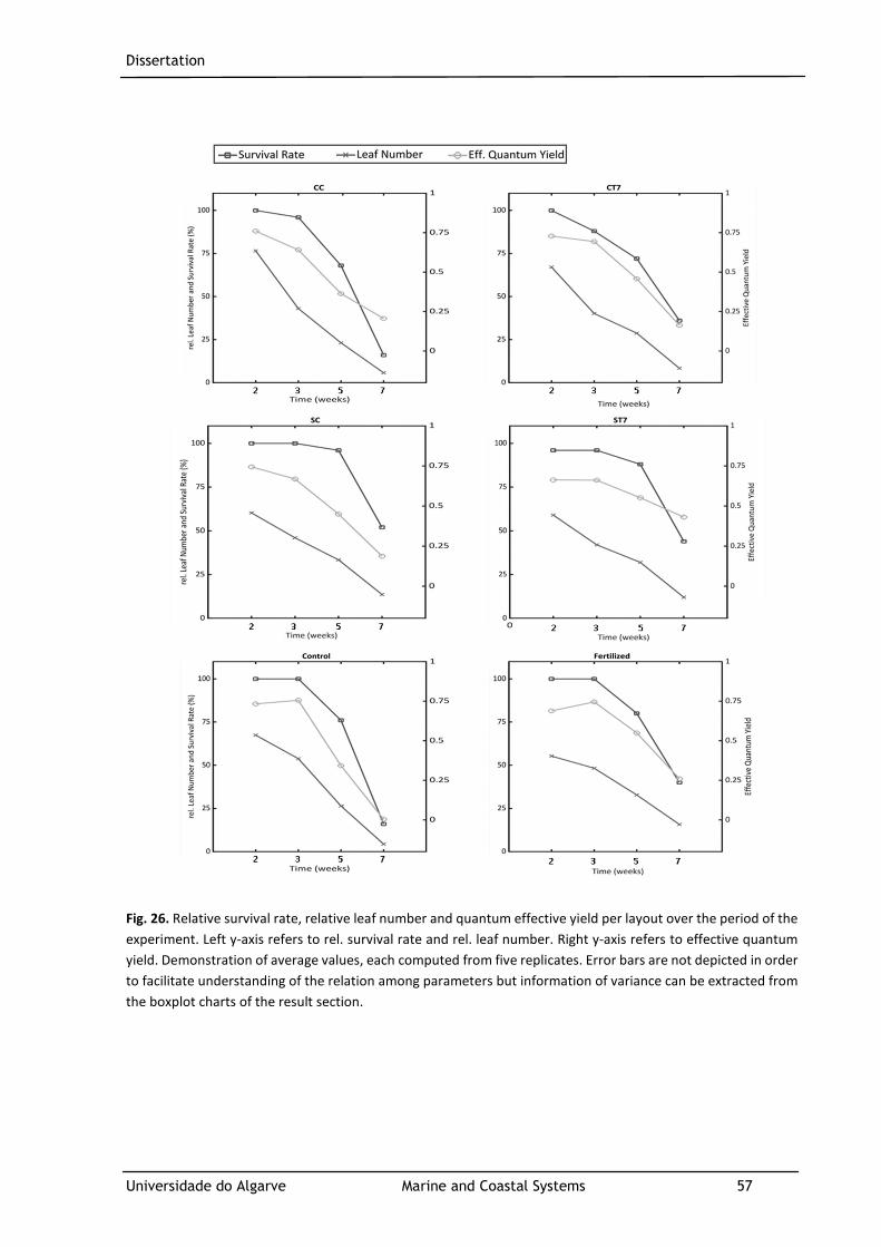
Dissertation
Universidade do Algarve Marine and Coastal Systems 57
Fig. 26. Relative survival rate, relative leaf number and quantum effective yield per layout over the period of the
experiment. Left y-axis refers to rel. survival rate and rel. leaf number. Right y-axis refers to effective quantum
yield. Demonstration of average values, each computed from five replicates. Error bars are not depicted in order
to facilitate understanding of the relation among parameters but information of variance can be extracted from
the boxplot charts of the result section.

Dissertation
Universidade do Algarve Marine and Coastal Systems 58
Dissertation
Universidade do Algarve Marine and Coastal Systems 59
6 DISUSSION
6.1 BIODEGRADATION
Physical properties of the individual fibers as well as their processing into woven textiles
influenced the outcome of the biodegradation experiments. Coir fibers are considered the
most durable fiber (Lekha, 2004), agreeing with the marginal weight loss of both coir net
layouts. Increase in weight might be associated to the very porous structure of the net and
mats, making it easily accessible for microorganisms or sediment accumulation, obscuring
weight loss through degradation. This assumption agrees with findings from Di Franco et al.,
(2004), who claimed that weight determination is sensitive to errors due to the prior described
cause. Contrasting behavior was observed in sisal layouts leading to the assumption that the
dense grid did not allow any accumulation of biomass or sediments and resulting in an initially
measurable weight loss. Because of the wide grid of the jute mesh entrapment of any kind
within the substrates might have been possible, indicated by the initial increase in weight,
comparable to the coir net layouts. Nevertheless, the wide grid could not prevent eventual
weight loss, leaving the mats unprotected and degrade faster than the CC and CT7 layouts. It
appeared that the threshold of initiating biodegradation with regard to weight loss was
reached after eight weeks for jute and sisal net layouts, which both experienced sudden drops
in weight after that point of time. In the following month weight dropped more rapidly than
before, implying that, as soon the degradation process is initiated, it proceeds much faster
than at the start and, thus is not a linear function of exposure.
Tensile strength loss analysis was only applied to the nets, as the machine brackets
hold on to the outer layer of the substrate (net). Mats were not relevant for this analysis since
their purpose was not to increase stability but serve as rooting ground for the shoots. Tensile
strength varied between the layouts from the beginning due to differences in yarn thickness
as well as weaving design. Mechanical properties of textile fabrics are influenced by the
individual fiber properties and subsequently modified by the conversion into yarns and into
the final fabric (Saiman et al., 2014).During tensile strength testing the longitudinal applied
load foremost attacks the fiber friction among fibers, followed by the elongation of the yarns
(Saiman et al., 2014).Furthermore, force at break increases with weft yarn density (Nassif,

Dissertation
Universidade do Algarve Marine and Coastal Systems 60
2012).The original superior performance of the sisal net layouts can be attributed to its high
tensile strength of the individual fibers (Haque et al., 2015) in combination with the high
density weft design of the net. Coir fibers possess lower tensile strength than jute fibers (Wu
et al., 2020). Yet, tensile strength of the coir net fabrics was far better than tensile strength of
the jute nets probably due to the very low density of yarn count within the jute nets, leading
to inferior capability of withstanding the applied load. Nevertheless, the baseline of tensile
strength of the individual layouts did not influence their over time performance after burial.
Although sisal layouts possessed the highest tensile strength in the controls, they experienced
the most significant loss in tensile strength over time. The decrease of tensile strength as a
function of exposure of these layouts was associated with the weight loss. Within both
variables sisal nets reduced performance in the first week and subsequently stayed constant
until the 8th week of the experiment, in which another significant drop in performance was
discovered. The magnitude of diminution between the 4th and the 8th week ranged around
1.3-2x for both parameters, demonstrating analogous reduction. Additionally, oxygen
consumption rates correspond to the behavior of the mechanical parameters. Though,
differences between the first and second month were not significant (p=0.051) a clear upward
trend of OCR was observed, initiated after eight weeks alike weight loss and tensile strength
loss. Furthermore, differences in variance between the first four weeks and the following
(Permdisp p=0.001, Appendix 7) might have influenced the PERMANOVA results, and
therefore not indicating the significance of difference between these two time intervals.
Tensile strength loss in jute nets behaved in a similar matter, in which a sudden decrease of
strength was revealed in the last two months of the experiment. According to a study from
Saha et al., (2012) jute fabrics, exposed to a 3 % NaCl aqueous solution for 120 days, were left
with 15 % of their original tensile strength. Tensile strength for jute layouts in this study
reduced by approx. 70% after a period of 84 days, comparable to the results from this study.
The decrease of tensile strength was more pronounced even, possibly due to the additional
component of the burial. Yet, although weight reduction between jute net layouts was the
same after two months, tensile strength loss was not induced in JC layouts up until the third
month, whereas tensile strength reduced half already after two months in JT7 structures.
According to these findings tensile strength reduction clearly was influenced by another factor
than just weight loss. Oxygen consumption rate ranged in similar magnitudes for both jute net
layouts, implying comparable aerobic microbial activity. Hence, OCR was not the influencing

Dissertation
Universidade do Algarve Marine and Coastal Systems 61
factor on the variance in tensile strength loss between the layouts. Aerobic microbial activity
appeared to be rather independent from the mechanical properties for jute net layouts until
the final stage of the experiment. Complementary to the tensile strength loss in JC, an increase
of OCR was recorded. Nevertheless, other conformities among the parameters for jute net
layouts were not identified. Tensile strength loss in coir net layouts followed, like sisal net
layouts, the pattern of the weight loss. After eight weeks tensile performance of CT7 layouts
lowered 1.3x compared to the first month, alike the weight and, increased in the same
magnitude as it lowered after twelve weeks for tensile strength and weight. Also, CC layouts
dropped in weight and tensile strength simultaneously after three months, indicating
correlating behavior between tensile strength and weight loss. The overall OCR was rather low
in coir net textiles compared to the other layouts. The high lignin content in the coir fibers
results in protection of the cellulose, thus protection from chemical and biological
deterioration (Rajan et al., 2005), which was supported by the findings of this study.
Microorganisms are more susceptible to degrade fibers with higher cellulose and
hemicellulose components and only few microorganisms are capable of decomposing lignin
(Rajan et al., 2005). Composition of cellulose, hemicellulose and lignin is comparable between
sisal and jute fibers, potentially explaining the similar degradation behavior of these two
layouts.
Generally, the increased variance in OCR might have led to misinterpretation of final
results questionable, which though, is an inherent occurrence in biological investigations
(Hicks et al., 2020). Possible reason for the high variance in the tensile strength in coir net and
jute net layouts might be the inconsistency of the thickness of yarns, therefore forces
distribute differently throughout the samples among replicates. This assumption is supported
by the low variance in sisal layouts, attributed to the very consistent net it provides. Weight
loss appeared to be less affected by spreading, wherefore results are more reliable.
Improvement of results can be achieved by using an increased sample size and thereby,
achieve a more consistent pattern.
This study showed that, the biodegradation of fibers from natural derivates requires a
certain time of response until the degradation process is induced. All layouts were rather
stable in their physical properties along with aerobic microbial activity and declined
significantly in performance after a threshold of two or three months. Furthermore, it was
Dissertation
Universidade do Algarve Marine and Coastal Systems 62
proven that, the chemical composition of the fibers was responsible for the degree of
degradation of the different layouts, as the two opposing weave designs of a high-density sisal
mesh appeared to degrade in similar manner as a low-density jute mesh. Moreover, this work
showcased that textile substrates degrade more rapidly submerged in the marine
environment than in terrestrial. Sisal fibers degrade within 24-36 months in contact with soil
(The East Africa Sisal Company Ltd.). This study revealed, that if sisal would degrade at the
same rate as the past three months, a full weight loss of less in twelve months would be
achieved. Weight loss in coir textiles proceeds much slower than the given 36-48 months rate
from literature (Greenfix). Yet, tensile strength was reduced by avg. 30 % after three months,
whereas according to Sumi et al., (2018) coir buried in sand lacked 63 % of tensile strength
after one year, corresponding to the initial statement that saline environment catalyzes
degradation. According to a study from Arshad & Mujahid, (2011) jute lost 40 % of its weight
after three months. In the case of this study structures composed with jute nets only degraded
by 15 % during that time period. Though, due to the wide grid of the jute net, weight decrease
affected the interior coir mats directly, therefore it is not clear how much the jute net itself
degraded, as it only took a small weight percentage of the overall weight of the sandwich
structure. It was expected that the high resistance of sisal to saltwater would result in a
superior performance of these layouts above the others with regard to biodegradation and
that the enclosed net structure would decrease microbial attack. This study demonstrated
that despite the high resistance of sisal fibers towards saline water, biodegradation was more
pronounced than in coir net textiles and was more similar to jute net layouts, disproving with
expectations. Predictions about the mats were not met. Type 7 mat did not experience
increased biodegradation compared to the cocomat. In fact, no distinction between the two
types of nonwovens was discovered.

Dissertation
Universidade do Algarve Marine and Coastal Systems 63
6.2 MESOCOSM
During the course of the experiments shoot integrity and number decreased in all treatments,
wherefore it was examined in which setting shoots were the healthiest over time and survived
the longest. Mortality was potentially caused by immoderate water temperature. Annual
average water temperatures around the donor meadow (Culatra island) range between 18 °C
– 20°C (Newton & Mudge, 2003) , approx. 8°C lower than the temperature in the tanks.
Additionally, minimum light requirements for Zostera marina, which, according to Eriander,
(2017), account for approx. 1875 lux, were only met at the southwest facing tanks. Though,
differences among replicates were not associated with their location in the tanks. Another
assumption is that, the damaged of the leaf puncturing was to severe, leaving shoots unable
to recover. Leaves turned brown from the puncture on towards the top and subsequently the
entire leave. Therefore, the measurement of leaf elongation could not be executed further
after three weeks into the experiment. Repuncturing also failed, since leaves turned brown
shortly after again. Hence, leaf elongation was excluded from the parameters.
Superior performance was observed in sisal layouts, in which shoots appeared to
undergo slowest degradation along with even some recovery towards the end of the
experiment. Mortality rate was lowest in these layouts, resulting in an increased leaf number.
Furthermore, shoots developed the highest number of new leaves and even root segment
elongation was observed in shoots, incorporated into SC fabrics, which, though was not
statistically proven. On the contrary, coir layouts offered the lowest support for shoots,
indicated by the inferior results of all parameters with CT7 layouts performing slightly better
than CC layouts. Shoots in controls did not appear to grow well either, leading to the
assumption, that a mesh with a certain thread density, and thus supporting system, can result
in better growth such as the sisal net. Despite these findings, fertilized shoots, which were not
growing on a carrier fabric, featured lower deterioration in their morphological appearance
than shoots growing on coir nets. Hence, the study demonstrated that the textile design,
especially thread density, along with the material selection are vital factors in the
development of textiles fostering shoot stabilization and growth, which was also showcased
in a study from Keune, (2017). The coir grid possibly did not supply sufficient support for the
shoots due to its lower thread density. Therefore, many leaves were lost from which the
Dissertation
Universidade do Algarve Marine and Coastal Systems 64
shoots could not recover and died eventually. Yet, as hydrodynamics were not mimicked in
this experiment, the stabilizing function of the meshes was not analyzed empirically and
hence, fertilized shoots possibly might behave inferior than coir net layouts outside laboratory
conditions. Contrary to this study, findings from other research suggest that coarse weave
meshes are more suitable for transplants of recruits and shoots as the rough surface of the
mesh facilitates root anchoring (Irving et al., 2010; Tanner et al., 2014; O'Brien, 2019). Yet, this
assumption is not applicable to this study as textile design along with function of the individual
substrates (mesh, mat) differed among studies. The function of the mesh in this study was to
provide enough support for the above ground parts of the as well as sediment stabilization
and strength for transport in future applications in the marine environment. A surface for root
entanglement was given by the mat. Thus, this work demonstrated that minor changes in
design alter the functionality immediately and must be tailored carefully to the particular
purpose such as rooting surface below ground or stabilization above ground of leaves and
shoots.
Furthermore, material degradation might affect shoot evolution via the provision of
compounds, that foster vegetation (Marczak et al., 2020). The in this study proven earlier
induced degradation process of the sisal fibers, resulted in earlier release of vegetation
supporting compounds into the mesocosm, supporting shoots in the production of new leaves
and maintaining the original shoot number as long as possible. Coir fibers are subject to slow
degradation thus, nutrients might be released in lower concentrations compared to the sisal
layouts and hence, the rate of newly developed leaves was the lowest in these layouts. Tanner
et al., (2014) claims that fast material degradation has adverse effect on shoot recruitment.
Lose parts of the textile disturb the shoots and put them under physical pressure. Because this
study was not executed in an environment exposed to hydrodynamical forces, this finding is
not applicable to this series of experiments and thus had no influence the results.
Nevertheless, the concern is valid and must be further investigated in future studies set
beyond laboratory conditions.
It was recognized that roots did not entangle into the mats during the period of the
experiment. As horizontal rhizome growth is rather slow (26 cm apex-1 yr-1(Marba et al.,
2004) it was not expected to observe interactions between the rhizomes and the mats.
Additionally, shoot development behaved contrary in the mats. Combined with the sisal net,
Dissertation
Universidade do Algarve Marine and Coastal Systems 65
ST7 performed inferior compared to SC, but, in combination with the coir net, CT7 showed
better results than CC. Hence, no distinction in performance related to the mats could be
made. Highest wet weight loss was identified in ST7 layouts as well as loss in root segment
length. Therefore, wet weight loss was attributed to loss in segment length due to the higher
wt.% of the roots than the leaves.
Most of the green leaves lost their integrity shortly after the start of the experiment
and turned into a brownish color. This was caused by the transformation of chlorophyll into
pheophytin, which is associated with external stressors such as increased temperature or light
(Aramrueang et al., 2019). Effective quantum yield decreased in shoots in all layouts,
associated with the loss of chlorophyll-a and possibly with down-regulation of photosynthesis
due to low irradiance conditions (Beer et al., 1998). Shoots in coir layouts and controls
possessed very low to absent effective quantum yield, respectively, indicating low
photosynthetic activity. Despite the increased development of new leaves in controls, yield
dropped abruptly after three weeks along with an analogous increase in mortality and loss in
leaf number, implying that new leaves did not survive in the environmental conditions of the
mesocosm and shoots could not recover. Highest effective quantum yield at the final stage of
the trials was found in shoots growing on ST7 layouts, even showing rates higher for some
replicates than at the beginning of the experiment, leading to the assumption that some of
the survived shoots were recovering and even thriving. Yet, an average decrease of effective
quantum yield was also noted for ST7 plants. Shoots incorporated into SC layouts featured
some increased yield, however on average lower photosynthesis was detected than in ST7
layouts. Still, rates were higher than in other treatments suggesting that the high survival rate
as well as increased leaf production rate in sisal layouts had positive influence on effective
quantum yield. Fertilized plants did not show any distinctive behavior from shoots
incorporated into sisal layouts, indicating that the fertilizer did not foster the integrity of the
plants to higher extent than the stabilization effect of the dense sisal mesh though higher than
the wider coir mesh. In summary the relation of effective quantum yield with the development
of new healthy leaves and the general mortality rate of the shoots is proven by the
continuously pattern of shoots growing on sisal mesh performing superior in all three
parameters, followed by fertilized shoots. Inferior performance was detected in shoots
growing on coir mesh and lowest plant integrity was found to be in controls.

Dissertation
Universidade do Algarve Marine and Coastal Systems 66
Dissertation
Universidade do Algarve Marine and Coastal Systems 67
7 CONCLUSION
In summary the most robust set up against biodegradation were layouts composed of coir
nets. Coconut fibers are proven to be very durable as well as the yarn thickness of the mesh
resulted in the improvement of tensile strength properties compared to the individual fibers.
It was discovered though that the retarded degradation of the material and the textile design
offered no positive effect on maintenance of the integrity nor growth of Zostera marina shoots
as performance of shoots planted without carrier substrate (controls) was similar. It was also
demonstrated that fertilized shoots, planted without carrier substrate, maintained better
integrity than shoots in coir meshes but worse than in sisal, emphasizing the importance of
right material and design selection. Despite the highest degradation rate, sisal layouts
possessed the highest initial and final tensile strength, resulting in less risk of failure during
transport and out-planting of seagrasses into the marine environment. Additionally, a more
rapid degradation might lead to nourishment of the shoots supporting growth. Moreover,
shoots incorporated into sisal meshes were proven to thrive in some replicates and overall
were in better state than shoots from other treatments.
Nevertheless, trials were conducted in controlled conditions for a short period of time
and were not subjected to hydrodynamic forces. It is possible that the rapid biodegradation
of the sisal mesh might be too pronounced over the long run, not giving shoots adequate time
to root into the sediment floor. Further research in the translation of these findings into the
open environment must be pursued.
Altogether, the null hypothesis was rejected as this work clearly depicted that a textile
carrier substrate can have positive influence on Zostera marina shoot integrity and that the
material and design of the substrate are vital factors to achieve successful restoration.

Dissertation
Universidade do Algarve Marine and Coastal Systems 68
Dissertation
Universidade do Algarve Marine and Coastal Systems 69
REFERENCES
Alloftextiles Online Limited (2015) Jute Fibers.
Aramrueang, N., Asavasanti, S. & Khanunthong, A. (2019) Leafy Vegetables. In: Integrated Processing Technologies for Food and Agricultural By-Products.
Elsevier, pp. 245–272.
Arshad, K. & Mujahid, M. (2011) Biodegradation of textile materials. Dissertation, Boras, The swedish school of textiles.
Barbier, E.B. (2017) Marine ecosystem services. Current Biology : CB, 27(11), R507-R510.
Basconi, L., Cadier, C. & Guerrero-Limón, G. (2020) Challenges in Marine Restoration Ecology: How Techniques, Assessment Metrics, and Ecosystem Valuation Can Lead to Improved Restoration Success. In: Jungblut, S., Liebich, V. & Bode-Dalby, M. (Eds.) YOUMARES 9 - The Oceans: Our Research, Our Future.
Springer International Publishing: Cham, pp. 83–99.
Bastyan, G.R. & Cambridge, M.L. (2008) Transplantation as a method for restoring the seagrass Posidonia australis. Estuarine, Coastal and Shelf Science, 79(2), 289–299.
Bayraktarov, E., Saunders, M.I., Abdullah, S., Mills, M., Beher, J. & Possingham, H.P. et al. (2016) The cost and feasibility of marine coastal restoration. Ecological Applications : a Publication of the Ecological Society of America, 26(4), 1055–1074.
Bedulli, C., Lavery, P.S., Harvey, M., Duarte, C.M. & Serrano, O. (2020) Contribution of Seagrass Blue Carbon Toward Carbon Neutral Policies in a Touristic and Environmentally-Friendly Island. Frontiers in Marine Science, 7, 338.
Beer, S., Vilenkin, B., Weil, A., Veste, M., Susel, L. & Eshel, A. (1998) Measuring photosynthetic rates in seagrasses by pulse amplitude modulated (PAM) fluorometry. Marine Ecology Progress Series, 174, 293–300.
Billingham, Reusch, T.B.H., Alberto, F. & Serrão, E.A. (2003) Is asexual reproduction more important at geographical limits? A genetic study of the seagrass Zostera marina in the Ria Formosa, Portugal. Marine Ecology Progress
Series, 265, 77–83.
Blott, S.J. & Pye, K. (2001) GRADISTAT: a grain size distribution and statistics package for the analysis of unconsolidated sediments. Earth Surface Processes
and Landforms, 26(11), 1237–1248.
Borum, J., Duarte, C.M., Krause-Jensen, D. & Greve, T.M. (2004) European seagrasses: an introduction to monitoring and management.
Dissertation
Universidade do Algarve Marine and Coastal Systems 70
Boström, C., Baden, S., Bockelmann, A.-C., Dromph, K., Fredriksen, S. & Gustafsson, C. et al. (2014) Distribution, structure and function of Nordic eelgrass (Zostera marina) ecosystems: implications for coastal management and conservation. Aquatic Conservation : Marine and Freshwater Ecosystems, 24(3), 410–434.
Bui, H., Sebaibi, N., Boutouil, M. & Levacher, D. (2020) Determination and Review of Physical and Mechanical Properties of Raw and Treated Coconut Fibers for Their Recycling in Construction Materials. Fibers, 8(6), 37.
Byers, J.E., Cuddington, K., Jones, C.G., Talley, T.S., Hastings, A. & Lambrinos, J.G. et al. (2006) Using ecosystem engineers to restore ecological systems. Trends in Ecology & Evolution, 21(9), 493–500.
Chakraborty, S., Mumtahenah Siddiquee, K., Maksud Helali, D.M. & Gafur, M. A (2014) Investigation of an Optimum Method of Bio degradation Process for Jute Polymer Composites. American Journal of Engineering Research, 2014(03(01)), 200–206.
Chand, N., Tiwary, R.K. & Rohatgi, P.K. (1988) Bibliography Resource structure properties of natural cellulosic fibres ? an annotated bibliography. Journal of
Materials Science, 23(2), 381–387.
Chattopadhyay, B.C. & Chakravarty, S. (2009) Application of jute geotextiles as facilitator in drainage. Geotextiles and Geomembranes, 27(2), 156–161.
Christensen, P.B., Díaz Almela, E. & Diekmann, O. Can transplanting accelerate the recovery of seagrasses? In: European seagrasses: An introduction to monitoring
and management : a publication, pp. 77–82.
Cole, M. (2016) A novel method for preparing microplastic fibers. Scientific
Reports, 6, 34519.
Collier, C. (2004) Zostera capensis (Marine Eelgrass).
Cullen-Unsworth, L.C. & Unsworth, R.K.F. (2016) Strategies to enhance the resilience of the world's seagrass meadows. Journal of Applied Ecology, 53(4), 967–972.
Cunha, A.H., Assis, J. & Serrao, E.A. (2009) Estimation of available seagrass meadow area in Portugal for transplanting purposes. Journal of Coastal
Research, 2009(SI 56), 1100–1104.
Cunha, A.H., Assis, J.F. & Serrão, E.A. (2013) Seagrasses in Portugal: A most endangered marine habitat. Aquatic Botany, 104, 193–203.
Cunha, A.H., Marbá, N.N., van Katwijk, M.M., Pickerell, C., Henriques, M. & Bernard, G. et al. (2012) Changing Paradigms in Seagrass Restoration. Restoration Ecology, 20(4), 427–430.
Dissertation
Universidade do Algarve Marine and Coastal Systems 71
Daria, M., Krzysztof, L. & Jakub, M. (2020) Characteristics of biodegradable textiles used in environmental engineering: A comprehensive review. Journal of Cleaner
Production, 268, 122129.
Datta, U. (2007) Application of Jute Geotextiles. Journal of Natural Fibers, 4(3), 67–82.
Delefosse, M. & Kristensen, E. (2012) Burial of Zostera marina seeds in sediment inhabited by three polychaetes: Laboratory and field studies. Journal of Sea
Research, 71, 41–49.
Dennison, W.C., Orth, R.J., Moore, K.A., Stevenson, J.C., Carter, V. & Kollar, S. et al. (1993) Assessing Water Quality with Submersed Aquatic Vegetation. BioScience, 43(2), 86–94.
Descamp, P., Cornu, T., Bougerol, M., Boissery, P., Ferlat, C. & Delaruelle, G. et al. (2017a) Experimental Transplantation of Posidonia Oceanica. 13th
International MEDCOAST Congress on Coastal and Marine Sciences, Engineering,
Management and. Malta, 31.10.-4.11.2017.
Descamp, P., Cornu, T., Bougerol, M., Boissery, P., Ferlat, C. & Delaruelle, G. et al. (2017b) Experimental Transplantation of Posidonia Oceanica. 13th
International MEDCOAST Congress on Coastal and Marine Sciences, Engineering,
Management and. Malta, 31.10.-4.11.2017.
Deutsches Institut für Normung e.V. DIN EN 17228:2019-06: Kunststoffe_-
Biobasierte Polymere, Kunststoffe und Kunststoffprodukte_- Begriffe, Merkmale
und Kommunikation; Deutsche Fassung EN_17228:2019, Berlin. Beuth Verlag GmbH.
Dietz, L.J., Venkatasubramani, A.V., Müller-Eigner, A., Hrabe de Angelis, M., Imhof, A. & Becker, L. et al. (2019) Measuring and Interpreting Oxygen Consumption Rates in Whole Fly Head Segments. Journal of Visualized
Experiments : JoVE, (143).
DIN EN 13432:2000-12, Berlin. Beuth Verlag GmbH.
DIN EN ISO 11721-1:2001, Berlin. Beuth Verlag GmbH.
Duarte, C.M. (2001) Seagrasses. In: Encyclopedia of Biodiversity. Elsevier, pp. 540–550.
Eckert, C.G. (2001) The loss of sex in clonal plants. Evolutionary Ecology, 15(4-6), 501–520.
Encyclopedia Britannica (2020) Monocotyledon | plant.
Endres, H.-J. & Siebert-Raths, A. (2009) Technische Biopolymere:
Rahmenbedingungen, Marktsitutation, Herstellung, Aufbau und Eigenschaften. Hanser: München.
Erftemeijer, P.L.A. (2020) Guidelines for Seagrass Ecosystem Restoration in the
Western Indian Ocean Region.
Dissertation
Universidade do Algarve Marine and Coastal Systems 72
Eriander, L. (2016) Restoration and management of eelgrass (Zostera marina) on
the West Coast of Sweden. Department of Marine Sciences, Faculty of Science, University of Gothenburg: Göteborg.
Eriander, L. (2017) Light requirements for successful restoration of eelgrass (Zostera marina L.) in a high latitude environment – Acclimatization, growth and carbohydrate storage. Journal of Experimental Marine Biology and Ecology, 496, 37–48.
Eriander, L., Infantes, E., Olofsson, M., Olsen, J.L. & Moksnes, P.-O. (2016) Assessing methods for restoration of eelgrass (Zostera marina L.) in a cold temperate region. Journal of Experimental Marine Biology and Ecology, 479, 76–88.
Ferrario, F., Beck, M.W., Storlazzi, C.D., Micheli, F., Shepard, C.C. & Airoldi, L. (2014) The effectiveness of coral reefs for coastal hazard risk reduction and adaptation. Nature Communications, 5, 3794.
Ferretto, G., Vergés, A., Glasby, T.M., Poore, A.G., Sinclair, E. & Statton, J. et al. (2019) Threatened plant translocation case study: Posidonia australis (Strapweed), Posidoniaceae. Australasian Plant Conservation, (28), 24–26
FITR (2008) Faserbewehrter Boden – Faserbewehrung von feinkörnigen
Recyclingmaterialien und Aushubböden für eine Verwertung im Erd- und
Tiefbau.
Folk, R.L. & Ward, W.C. (1957) Brazos River bar [Texas]; a study in the significance of grain size parameters. SEPM Journal of Sedimentary Research, 27(1), 3–26.
Fonseca, M.S., Kenworthy, W.J. & Thayer, G.W. (1998) Guidelines for the
conservation and restoration of seagrasses in the United States and adjacent
waters. United States.
Food and Agriculture Organization of the United Nations Jute.
Ghosh, S.K., Bhattacharyya, R. & Mondal, M.M. (2017) Potential Applications of Open Weave Jute Geotextile (Soil Saver) in Meeting Geotechnical Difficulties. Procedia Engineering, 200(1), 200–205.
Greenfix Greenfix Erosion Control Blanket Type 7: tech-spec.
Guidi, L., Lo Piccolo, E. & Landi, M. (2019) Chlorophyll Fluorescence, Photoinhibition and Abiotic Stress: Does it Make Any Difference the Fact to Be a C3 or C4 Species? Frontiers in Plant Science, 10, 174.
Guimarães, M.H.M.E., Cunha, A.H., Nzinga, R.L. & Marques, J.F. (2012) The distribution of seagrass (Zostera noltii) in the Ria Formosa lagoon system and the implications of clam farming on its conservation. Journal for Nature
Conservation, 20(1), 30–40.
Häck, M. (2003) Optical measurement of oxygen concentration in water: APPLICATION REPORT PROCESS ANALYSISLDO.

Dissertation
Universidade do Algarve Marine and Coastal Systems 73
Halpern, B.S., Walbridge, S., Selkoe, K.A., Kappel, C.V., Micheli, F. & D'Agrosa, C. et al. (2008) A global map of human impact on marine ecosystems. Science (New
York, N.Y.), 319(5865), 948–952.
Haque, R., Saxena, M., Shit, S.C. & Asokan, P. (2015) Fibre-matrix adhesion and properties evaluation of sisal polymer composite. Fibers and Polymers, 16(1), 146–152.
Harrison, J.P., Boardman, C., O'Callaghan, K., Delort, A.-M. & Song, J. (2018a) Biodegradability standards for carrier bags and plastic films in aquatic environments: a critical review. Royal Society Open Science, 5(5), 171792.
Harrison, J.P., Boardman, C., O'Callaghan, K., Delort, A.-M. & Song, J. (2018b) Biodegradability standards for carrier bags and plastic films in aquatic environments: a critical review. Royal Society Open Science, 5(5), 171792.
Healabel. Coconut Fiber.
Heinz Walz GmbH (1998) UNDERWATER FLUOROMETERDIVING-PAM: Submersible PhotosynthesisYield Analyzer. Handbook of Operation.
Hicks, J., Dewey, J., Brandvain, Y. & Schuchardt, A. (2020) Development of the Biological Variation In Experimental Design And Analysis (BioVEDA) assessment. PloS One, 15(7), e0236098.
Hottle, Troy A.; Bilec, Melissa M.; Landis, Amy E. (2013): Sustainability assessments of bio-based polymers. In: Polymer Degradation and Stability 98 (9), S. 1898–1907.
IPBES (2019) Nature’s Dangerous Decline ‘Unprecedented’ Species Extinction Rates ‘Accelerating’: Current global response insufficient; ‘Transformative changes’ needed to restore and protect nature; Opposition from vested interests can be overcome for public good, personal communication.
Irving, A.D., Tanner, J.E. & Collings, G.J. (2014) Rehabilitating Seagrass by Facilitating Recruitment: Improving Chances for Success. Restoration Ecology, 22(2), 134–141.
Irving, A.D., Tanner, J.E., Seddon, S., Miller, D., Collings, G.J. & Wear, R.J. et al. (2010) Testing alternate ecological approaches to seagrass rehabilitation: links to life-history traits. Journal of Applied Ecology, 47(5), 1119–1127.
ISO 13934-1:1999 Textiles — Tensile properties of fabrics — Part 1: Determination of maximum force. Beuth Verlag GmbH.
Jones, C.G., Lawton, J.H. & Shachak, M. (1994) Organisms as Ecosystem Engineers. Oikos, 69(3), 373.
Keser, M., Swenarton, J.T., Vozarik, J.M. & Foertch, J.F. (2003) Decline in eelgrass (Zostera marina L.) in Long Island Sound near Millstone Point, Connecticut (USA) unrelated to thermal input. Journal of Sea Research, 49(1), 11–26.

Dissertation
Universidade do Algarve Marine and Coastal Systems 74
Koohestani, B., Darban, A.K., Mokhtari, P., Yilmaz, E. & Darezereshki, E. (2019) Comparison of different natural fiber treatments: a literature review. International Journal of Environmental Science and Technology, 16(1), 629–642.
Krumbein, W.C. (1934) Size Frequency Distributions of Sediments. SEPM Journal of
Sedimentary Research, Vol. 4.
Kuo, J. & Hartog, C.d. (2006) Seagrass Morphology, Anatomy, and Ultrastructure. In: SEAGRASSES: BIOLOGY, ECOLOGYAND CONSERVATION. Springer Netherlands: Dordrecht, pp. 51–87.
Lal, D., Sankar, N. & Chandrakaran, S. (2017) Effect of reinforcement form on the behaviour of coir geotextile reinforced sand beds. Soils and Foundations, 57(2), 227–236.
Larkum, A., Duarte, C.M. & Orth, R.J. (2006) Seagrasses;Biology, ecology and conservation. Springer: Dordrecht.
Law, A., Gaywood, M.J., Jones, K.C., Ramsay, P. & Willby, N.J. (2017) Using ecosystem engineers as tools in habitat restoration and rewilding: beaver and wetlands. The Science of the Total Environment, 605-606, 1021–1030.
LEKHA, K. & KAVITHA, V. (2006) Coir geotextile reinforced clay dykes for drainage of low-lying areas. Geotextiles and Geomembranes, 24(1), 38–51.
Lekha, K.R. (2004) Field instrumentation and monitoring of soil erosion in coir geotextile stabilised slopes—A case study. Geotextiles and Geomembranes, 22(5), 399–413.
Li, Y., Mai, Y.-W. & Ye, L. (2000) Sisal fibre and its composites: a review of recent developments. Composites Science and Technology, 60(11), 2037–2055.
Mahuya, G., Choudhury, P.K. & Sanyal, T. (2009) Suitability of natural fibers in geotextile applications.
Marba, N., Duarte, C.M., Alexandre, A. & Cabaco, S. (Eds.) (2004) How do seagrasses grow and spread ?
Marczak, D., Lejcuś, K., Grzybowska-Pietras, J., Biniaś, W., Lejcuś, I. & Misiewicz, J. (2020) Biodegradation of sustainable nonwovens used in water absorbing geocomposites supporting plants vegetation. Sustainable Materials and
Technologies, 26(1191), e00235.
Mukherjee, P.S. & Satyanarayana, K.G. (1984) Structure and properties of some vegetable fibres. Journal of Materials Science, 19(12), 3925–3934.
Narayan, S., Beck, M.W., Reguero, B.G., Losada, I.J., van Wesenbeeck, B. & Pontee, N. et al. (2016) The Effectiveness, Costs and Coastal Protection Benefits of Natural and Nature-Based Defences. PloS One, 11(5), e0154735.
Nassif, G.A.A. (2012) Effect of Weave Structure and Weft Density on the Physical and Mechanical Properties of Micro polyester Woven Fabrics. Journal of
American Science, (8), 947–952.
Dissertation
Universidade do Algarve Marine and Coastal Systems 75
Newton, A. & Mudge, S.M. (2003) Temperature and salinity regimes in a shallow, mesotidal lagoon, the Ria Formosa, Portugal. Estuarine, Coastal and Shelf
Science, 57(1-2), 73–85.
O'Brien, D. (2019) Improving Seagrass Production for Transplants: Micropropagation, adventitious root development, and artificial substrates. Dissertation, Faro, Universidade do Algarve.
Papageorgiou, G.C. & Govindjee (Eds.) (op. 2010) Chlorophyll a fluorescence: A
signature of photosynthesis. Springer: Dordrecht, Heidelberg, London.
Paulo, D., Cunha, A.H., Boavida, J., Serrão, E.A., Gonçalves, E.J. & Fonseca, M. (2019) Open Coast Seagrass Restoration. Can We Do It? Large Scale Seagrass Transplants. Frontiers in Marine Science, 6, 16.
Paulo, D., Diekmann, O., Ramos, A.A., Alberto, F. & Alvares Serrão, E. (2019) Sexual reproduction vs. clonal propagation in the recovery of a seagrass meadow after an extreme weather event. Scientia Marina, 83(4), 357.
Pavlovic, D., Nikolic, B., Djurovic, S., Waisi, H., Andjelkovic, A. & Marisavljevic, D. (2014) Chlorophyll as a measure of plant health: Agroecological aspects. Pesticidi i fitomedicina, 29(1), 21–34.
Pazzaglia, Jessica; Nguyen, Hung Manh; Santillán-Sarmiento, Alex; Ruocco, Miriam; Dattolo, Emanuela; Marín-Guirao, Lázaro; Procaccini, Gabriele (2021): The Genetic Component of Seagrass Restoration: What We Know and the Way Forwards. In: Water 13 (6), S. 829.
Perrow, M.R. & Davy, A.J. (2004) Restoration in practice. Cambridge Univ. Press: Cambridge.
Pickerell, C., Schott, S., Manzo, K., Udelson, B., Krupski, N. & Barbour, K. (2012) The Tortilla Method: Development and testing of a new Seagrass Planting Method.
Rajan, A., Senan, R.C., Pavithran, C. & Abraham, T.E. (2005) Biosoftening of coir fiber using selected microorganisms. Bioprocess and Biosystems Engineering, 28(3), 165–173.
Ralph, P.J. & Short, F.T. (2002) Impact of the wasting disease pathogen, Labyrinthula zosterae, on the photobiology of eelgrass Zostera marina. Marine
Ecology Progress Series, 226, 265–271.
Ramamoorthy, S.K., Skrifvars, M. & Persson, A. (2015) A Review of Natural Fibers Used in Biocomposites: Plant, Animal and Regenerated Cellulose Fibers. Polymer
Reviews, 55(1), 107–162.
Rey Benayas, J.M., Newton, A.C., Diaz, A. & Bullock, J.M. (2009) Enhancement of biodiversity and ecosystem services by ecological restoration: a meta-analysis. Science (New York, N.Y.), 325(5944), 1121–1124.
Dissertation
Universidade do Algarve Marine and Coastal Systems 76
Reynolds, P.L. (2013) Seagrass and Seagrass Beds. Smithsonian's National Museum
of Natural History, 28 February.
Ricart, A.M., York, P.H., Rasheed, M.A., Pérez, M., Romero, J. & Bryant, C.V. et al. (2015) Variability of sedimentary organic carbon in patchy seagrass landscapes. Marine Pollution Bulletin, 100(1), 476–482.
Riniatsih, I., Hartati, R., Endrawati, H., Mahendrajaya, R., Redjeki, S. & Widianingsih, W. (2018) The application of Environmental Friendly Technique For Seagrass Transplantation. IOP Conference Series: Earth and Environmental
Science, 116, 12103.
Robinson, W.O. (1927) THE DETERMINATION OF ORGANIC MATTER IN SOILS BY MEANS OF HYDROGEN PEROXIDE.
Röhr, M.E., Holmer, M., Baum, J.K., Björk, M., Boyer, K. & Chin, D. et al. (2018) Blue Carbon Storage Capacity of Temperate Eelgrass (Zostera marina ) Meadows. Global Biogeochemical Cycles, 32(10), 1457–1475.
Rosa, F., Gaspar, M., Rufino, M., Ferreira, O., Matias, A. & Brito, A. (2013) The influence of coastal processes on inner shelf sediment distribution: The Eastern Algarve Shelf (Southern Portugal). Geologica Acta, (11), 59–73.
Rossi, F., Gribsholt, B., Gazeau, F., Di Santo, V. & Middelburg, J.J. (2013) Complex Effects of Ecosystem Engineer Loss on Benthic Ecosystem Response to Detrital Macroalgae. PloS One, 8(6), e66650.
Saha, P., Roy, D., Manna, S., Adhikari, B., Sen, R. & Roy, S. (2012) Durability of transesterified jute geotextiles. Geotextiles and Geomembranes, 35, 69–75. Available from: https://doi.org/10.1016/j.geotexmem.2012.07.003.
Saiman, M.P., Wahab, M.S. & Wahit, M.U. (2014) The Effect of Fabric Weave on the Tensile Strength of Woven Kenaf Reinforced Unsaturated Polyester Composite. In: Ahmad, M.R. & Yahya, M.F. (Eds.) Proceedings of the International
Colloquium in Textile Engineering, Fashion, Apparel and Design 2014 (ICTEFAD
2014). Springer Singapore: Singapore, pp. 25–29.
Satyanarayana, K.G., Kulkarni, A.G. & Rohatgi, P.K. (1981) Structure and properties of coir fibres. Proc. Indian Acad. Sci. (Engg. Sci.), (Vol. 4), 419-436
Senga Green, D. Environmental impacts of plastic debris on marine ecosystems.
Royal Society of Chemistry.
Setchell, W.A. (1935) Geographic Elements of the Marine Flora of the North Pacific Ocean. The American Naturalist, 69(725), 560–577.
Short, F., Carruthers, T., Dennison, W. & Waycott, M. (2007) Global seagrass distribution and diversity: A bioregional model. Journal of Experimental Marine
Biology and Ecology, 350(1-2), 3–20.
Short, F.T., Burdick, D., Granger, S. & Nixon, S.W. (1996) Long-term decline in eelgrass, Zostera marina L. linked to increased housing development. Seagrass

Dissertation
Universidade do Algarve Marine and Coastal Systems 77
Biology:Proceedings of an international workshop. Rottnest Island, Australia, 25.-29. January, 1996.
Short, F.T. & Coles, R.G. (Eds.) (2001) Global Seagrass Research Methods. Elsevier.
Shruti, V.C. & Kutralam-Muniasamy, G. (2019) Bioplastics: Missing link in the era of Microplastics. Science of The Total Environment, 697, 134139.
Singh, H., Inder Preet Singh, J., Singh, S., Dhawan, V. & Kumar Tiwari, S. (2018) A Brief Review of Jute Fibre and Its Composites. Materials Today: Proceedings, 5(14), 28427–28437.
Siracusa, V. (2019) Microbial Degradation of Synthetic Biopolymers Waste. Polymers, 11(6).
Solana-Arellano, M.E., Echavarria-Heras, H.A. & Ibarra-Obando, S.E. (1997) Leaf-size Dynamics forZostera marinaL. in San Quintin Bay, México: a Theoretical Study. Estuarine, Coastal and Shelf Science, 44(3), 351–359.
Statton, J., Gustin-Craig, S., Dixon, K.W. & Kendrick, G.A. (2015) Edge Effects along a Seagrass Margin Result in an Increased Grazing Risk on Posidonia australis Transplants. PloS One, 10(10), e0137778.
Sülar, V. & Devrim, G. (2019) Biodegradation Behaviour of Different Textile Fibres: Visual, Morphological, Structural Properties and Soil Analyses. Fibres and
Textiles in Eastern Europe, 27(1(133)), 100–111.
Sumi, S., Unnikrishnan, N. & Mathew, L. (2018) Durability studies of surface-modified coir geotextiles. Geotextiles and Geomembranes, 46(6), 699–706.
Tan, Y.M., Dalby, O., Kendrick, G.A., Statton, J., Sinclair, E.A. & Fraser, M.W. et al. (2020) Seagrass Restoration Is Possible: Insights and Lessons From Australia and New Zealand. Frontiers in Marine Science, 7, 367.
Tanner, J.E., Irving, A.D., Fernandes, M., Fotheringham, D., McArdle, A. & Murray-Jones, S. (2014) Seagrass rehabilitation off metropolitan Adelaide: a case study of loss, action, failure and success. Ecological Management & Restoration, 15(3), 168–179.
The East Africa Sisal Company Ltd. Geo-Sisal Peatsock: Data Sheet.
Thyavihalli Girijappa, Y.G., Mavinkere Rangappa, S., Parameswaranpillai, J. & Siengchin, S. (2019) Natural Fibers as Sustainable and Renewable Resource for Development of Eco-Friendly Composites: A Comprehensive Review. Frontiers in
Materials, 6.
TUTIN, T.G. (1938) THE AUTECOLOGY OF ZOSTERA MARINA IN RELATION TO ITS WASTING DISEASE. New Phytologist, 37(1), 50–71.
Unsworth, R.K.F., Bertelli, C.M., Cullen-Unsworth, L.C., Esteban, N., Jones, B.L. & Lilley, R. et al. (2019) Sowing the Seeds of Seagrass Recovery Using Hessian Bags. Frontiers in Ecology and Evolution, 7.
Dissertation
Universidade do Algarve Marine and Coastal Systems 78
van Katwijk, M.M., Thorhaug, A., Marbà, N., Orth, R.J., Duarte, C.M. & Kendrick, G.A. et al. (2016) Global analysis of seagrass restoration: the importance of large-scale planting. Journal of Applied Ecology, 53(2), 567–578.
Vos, J.M. de, Joppa, L.N., Gittleman, J.L., Stephens, P.R. & Pimm, S.L. (2015) Estimating the normal background rate of species extinction. Conservation
Biology : the Journal of the Society for Conservation Biology, 29(2), 452–462.
Wageningen University & Research (n.a.) Pulse-Amplitude-Modulation (PAM).
Waycott, M., Duarte, C.M., Carruthers, T.J.B., Orth, R.J., Dennison, W.C. & Olyarnik, S. et al. (2009) Accelerating loss of seagrasses across the globe threatens coastal ecosystems. Proceedings of the National Academy of Sciences
of the United States of America, 106(30), 12377–12381.
Wendländer, N.S., Troels Lange, Rod M. Connolly, Erik Kristensen, Ryan M. Pearson & Thomas Valdemarsen et al. (2019) Assessing methods for restoring seagrass (Zostera muelleri) in Australia’s subtropical waters. Marine and Freshwater
Research, 71(8), 996–1005.
Wentworth, C.K. (1922) A Scale of Grade and Class Terms for Clastic Sediments. The Journal of Geology, 30(5), 377–392.
Williams, S.L. (2007) Introduced species in seagrass ecosystems: Status and concerns. Journal of Experimental Marine Biology and Ecology, 350(1-2), 89–110.
Wilson, A.M.W. & Forsyth, C. (2018) Restoring near-shore marine ecosystems to enhance climate security for island ocean states: Aligning international processes and local practices. Marine Policy, 93(4), 284–294.
Wu, H., Yao, C., Li, C., Miao, M., Zhong, Y. & Lu, Y. et al. (2020) Review of Application and Innovation of Geotextiles in Geotechnical Engineering. Materials
(Basel, Switzerland).
Xu, S., Zhou, Y., Wang, P., Wang, F., Zhang, X. & Gu, R. (2016) Salinity and temperature significantly influence seed germination, seedling establishment, and seedling growth of eelgrass Zostera marina L. PeerJ, 4, e2697.
Yu, C. (2015) Natural Textile Fibres. In: Textiles and Fashion. Elsevier, pp. 29–56.
Zambrano, M.C., Pawlak, J.J., Daystar, J., Ankeny, M., Goller, C.C. & Venditti, R.A. (2020) Aerobic biodegradation in freshwater and marine environments of textile microfibers generated in clothes laundering: Effects of cellulose and polyester-based microfibers on the microbiome. Marine Pollution Bulletin, 151, 110826.
Zedler, J.B. (2007) Success: An Unclear, Subjective Descriptor of Restoration Outcomes. Ecological Restoration, 25(3), 162–168.
Zhou, Y., Liu, P., Liu, B., Liu, X., Zhang, X. & Wang, F. et al. (2014) Restoring eelgrass (Zostera marina L.) habitats using a simple and effective transplanting technique. PloS One, 9(4), e92982.
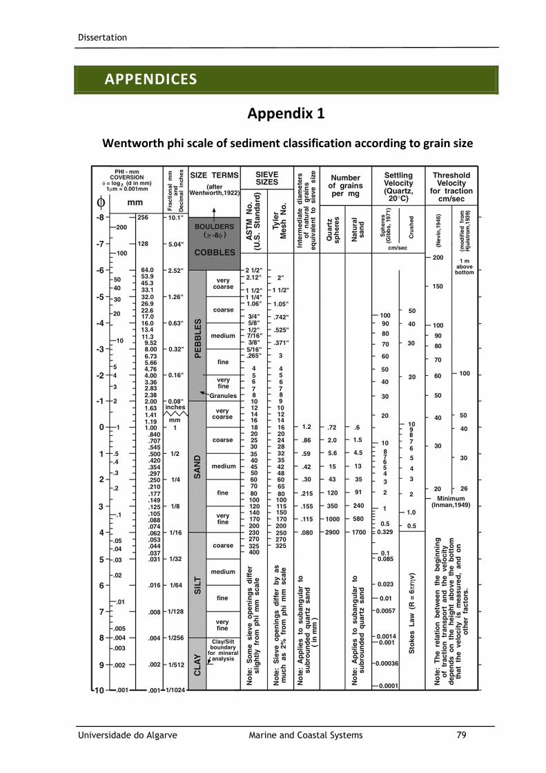
Dissertation
Universidade do Algarve Marine and Coastal Systems 79
APPENDICES
Appendix 1
Wentworth phi scale of sediment classification according to grain size
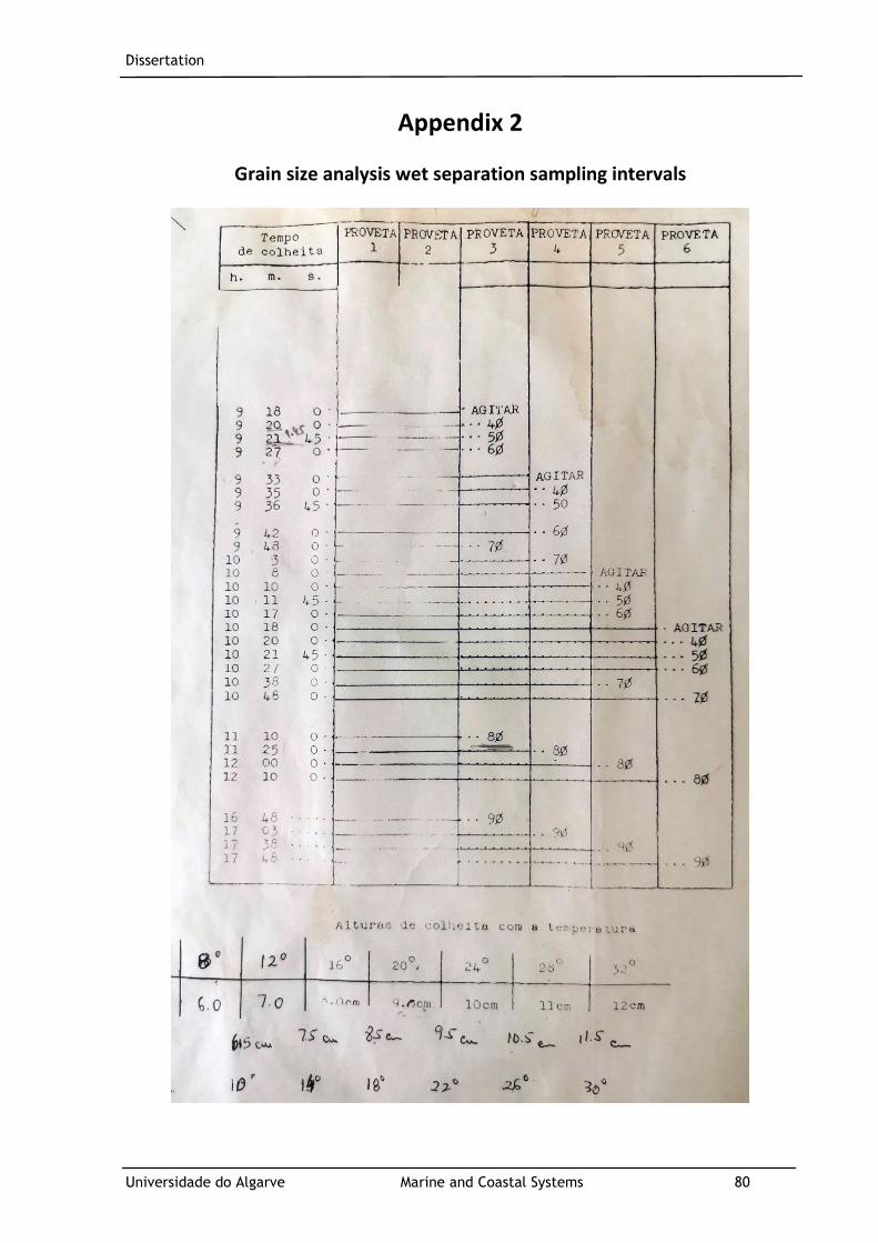
Dissertation
Universidade do Algarve Marine and Coastal Systems 80
Appendix 2
Grain size analysis wet separation sampling intervals
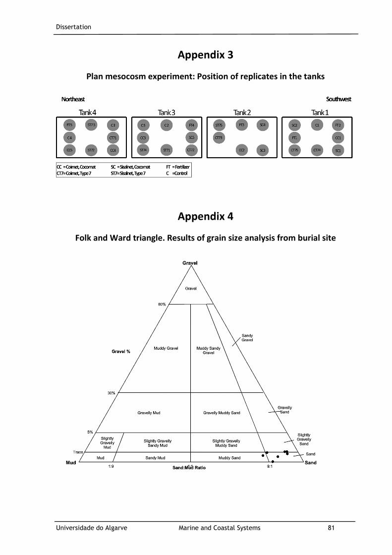
Dissertation
Universidade do Algarve Marine and Coastal Systems 81
Appendix 3
Plan mesocosm experiment: Position of replicates in the tanks
Appendix 4
Folk and Ward triangle. Results of grain size analysis from burial site
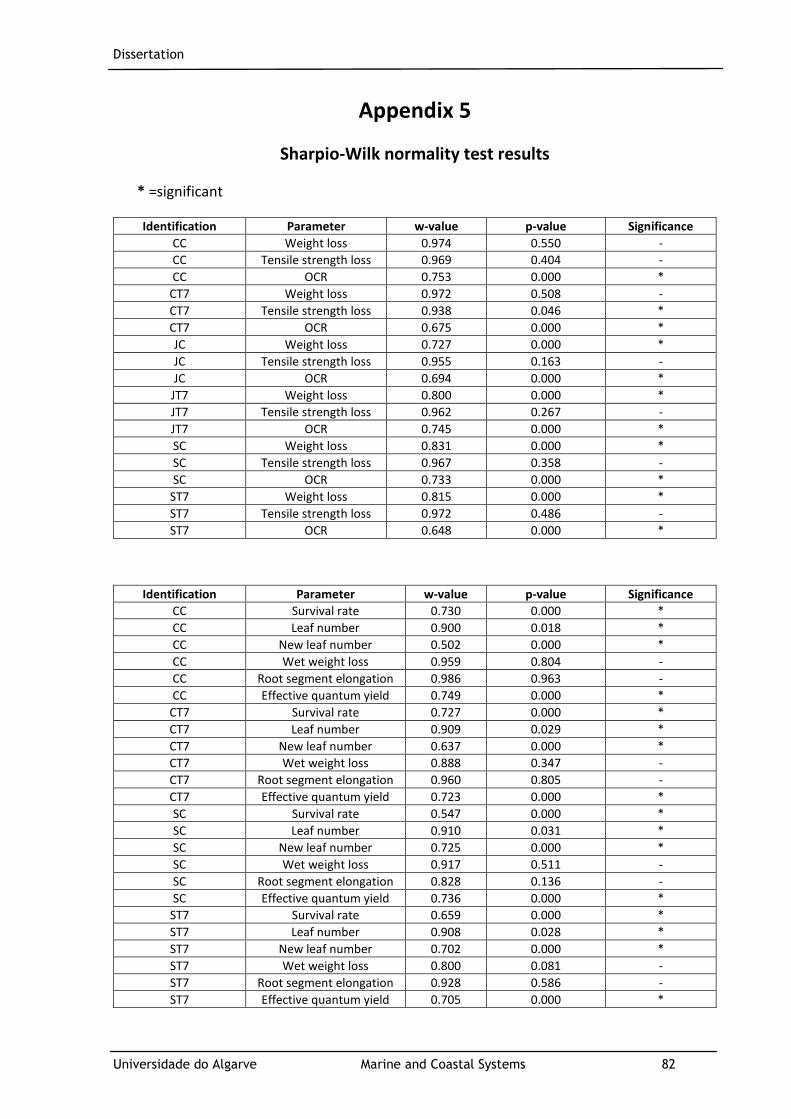
Dissertation
Universidade do Algarve Marine and Coastal Systems 82
Appendix 5
Sharpio-Wilk normality test results
* =significant
Identification Parameter w-value p-value Significance
CC Weight loss 0.974 0.550 -
CC Tensile strength loss 0.969 0.404 -
CC OCR 0.753 0.000 *
CT7 Weight loss 0.972 0.508 -
CT7 Tensile strength loss 0.938 0.046 *
CT7 OCR 0.675 0.000 *
JC Weight loss 0.727 0.000 *
JC Tensile strength loss 0.955 0.163 -
JC OCR 0.694 0.000 *
JT7 Weight loss 0.800 0.000 *
JT7 Tensile strength loss 0.962 0.267 -
JT7 OCR 0.745 0.000 *
SC Weight loss 0.831 0.000 *
SC Tensile strength loss 0.967 0.358 -
SC OCR 0.733 0.000 *
ST7 Weight loss 0.815 0.000 *
ST7 Tensile strength loss 0.972 0.486 -
ST7 OCR 0.648 0.000 *
Identification Parameter w-value p-value Significance
CC Survival rate 0.730 0.000 *
CC Leaf number 0.900 0.018 *
CC New leaf number 0.502 0.000 *
CC Wet weight loss 0.959 0.804 -
CC Root segment elongation 0.986 0.963 -
CC Effective quantum yield 0.749 0.000 *
CT7 Survival rate 0.727 0.000 *
CT7 Leaf number 0.909 0.029 *
CT7 New leaf number 0.637 0.000 *
CT7 Wet weight loss 0.888 0.347 -
CT7 Root segment elongation 0.960 0.805 -
CT7 Effective quantum yield 0.723 0.000 *
SC Survival rate 0.547 0.000 *
SC Leaf number 0.910 0.031 *
SC New leaf number 0.725 0.000 *
SC Wet weight loss 0.917 0.511 -
SC Root segment elongation 0.828 0.136 -
SC Effective quantum yield 0.736 0.000 *
ST7 Survival rate 0.659 0.000 *
ST7 Leaf number 0.908 0.028 *
ST7 New leaf number 0.702 0.000 *
ST7 Wet weight loss 0.800 0.081 -
ST7 Root segment elongation 0.928 0.586 -
ST7 Effective quantum yield 0.705 0.000 *
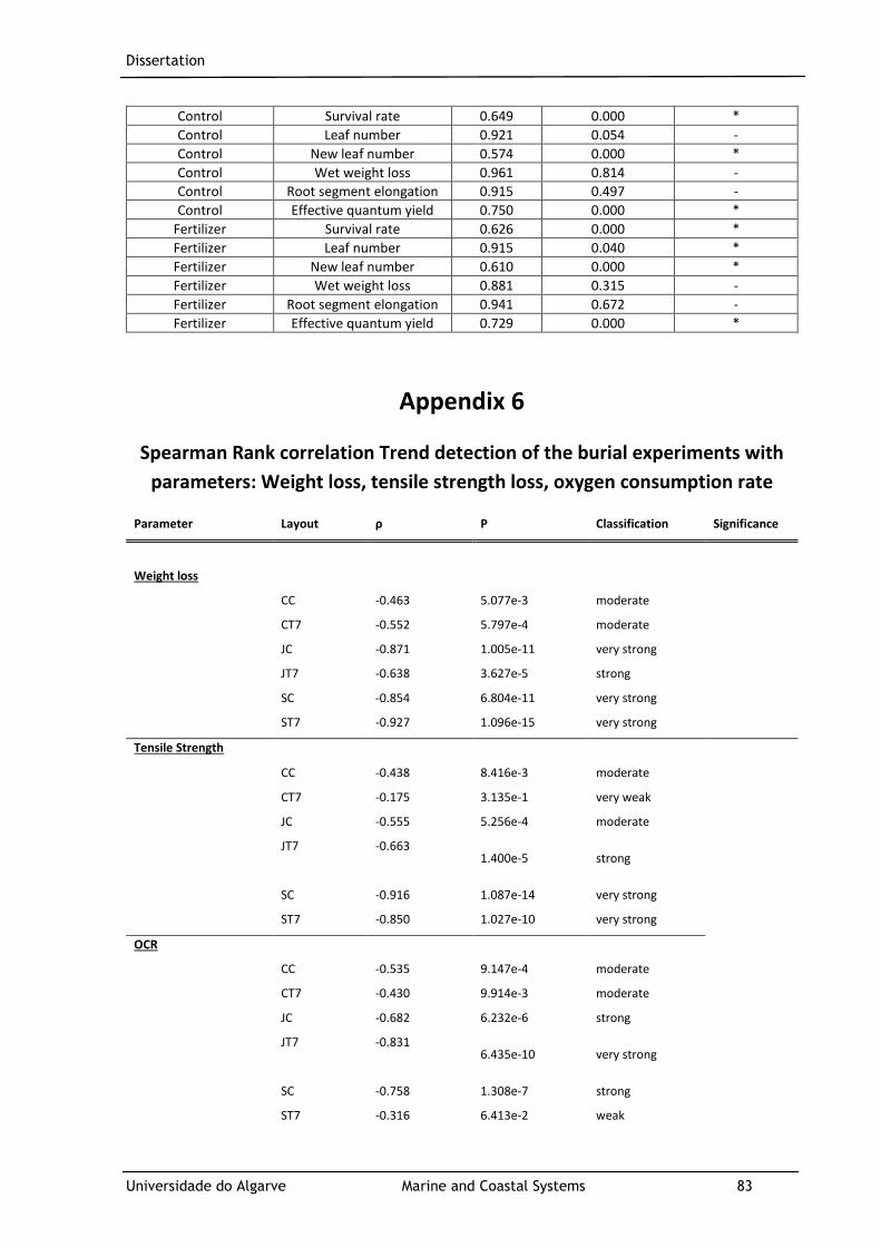
Dissertation
Universidade do Algarve Marine and Coastal Systems 83
Control Survival rate 0.649 0.000 *
Control Leaf number 0.921 0.054 -
Control New leaf number 0.574 0.000 *
Control Wet weight loss 0.961 0.814 -
Control Root segment elongation 0.915 0.497 -
Control Effective quantum yield 0.750 0.000 *
Fertilizer Survival rate 0.626 0.000 *
Fertilizer Leaf number 0.915 0.040 *
Fertilizer New leaf number 0.610 0.000 *
Fertilizer Wet weight loss 0.881 0.315 -
Fertilizer Root segment elongation 0.941 0.672 -
Fertilizer Effective quantum yield 0.729 0.000 *
Appendix 6
Spearman Rank correlation Trend detection of the burial experiments with
parameters: Weight loss, tensile strength loss, oxygen consumption rate
Parameter Layout ρ P Classification Significance
Weight loss
CC -0.463 5.077e-3 moderate
CT7 -0.552 5.797e-4 moderate
JC -0.871 1.005e-11 very strong
JT7 -0.638 3.627e-5 strong
SC -0.854 6.804e-11 very strong
ST7 -0.927 1.096e-15 very strong
Tensile Strength
CC -0.438 8.416e-3 moderate
CT7 -0.175 3.135e-1 very weak
JC -0.555 5.256e-4 moderate
JT7 -0.663 1.400e-5 strong
SC -0.916 1.087e-14 very strong
ST7 -0.850 1.027e-10 very strong
OCR
CC -0.535 9.147e-4 moderate
CT7 -0.430 9.914e-3 moderate
JC -0.682 6.232e-6 strong
JT7 -0.831 6.435e-10 very strong
SC -0.758 1.308e-7 strong
ST7 -0.316 6.413e-2 weak

Dissertation
Universidade do Algarve Marine and Coastal Systems 84
Appendix 7
Profile tensile strength test INSTRON
Table 9. Legend - Translation of graph labels
German English
Kraft Force Verfahrensweg Procedural path Kraft bei Zugfestigkeit Tensile strength Zugspannung bei Zugfestigkeit Tension at force at break Zugverfahrensweg bei Zugfestikeit Proceduaral path at force at break
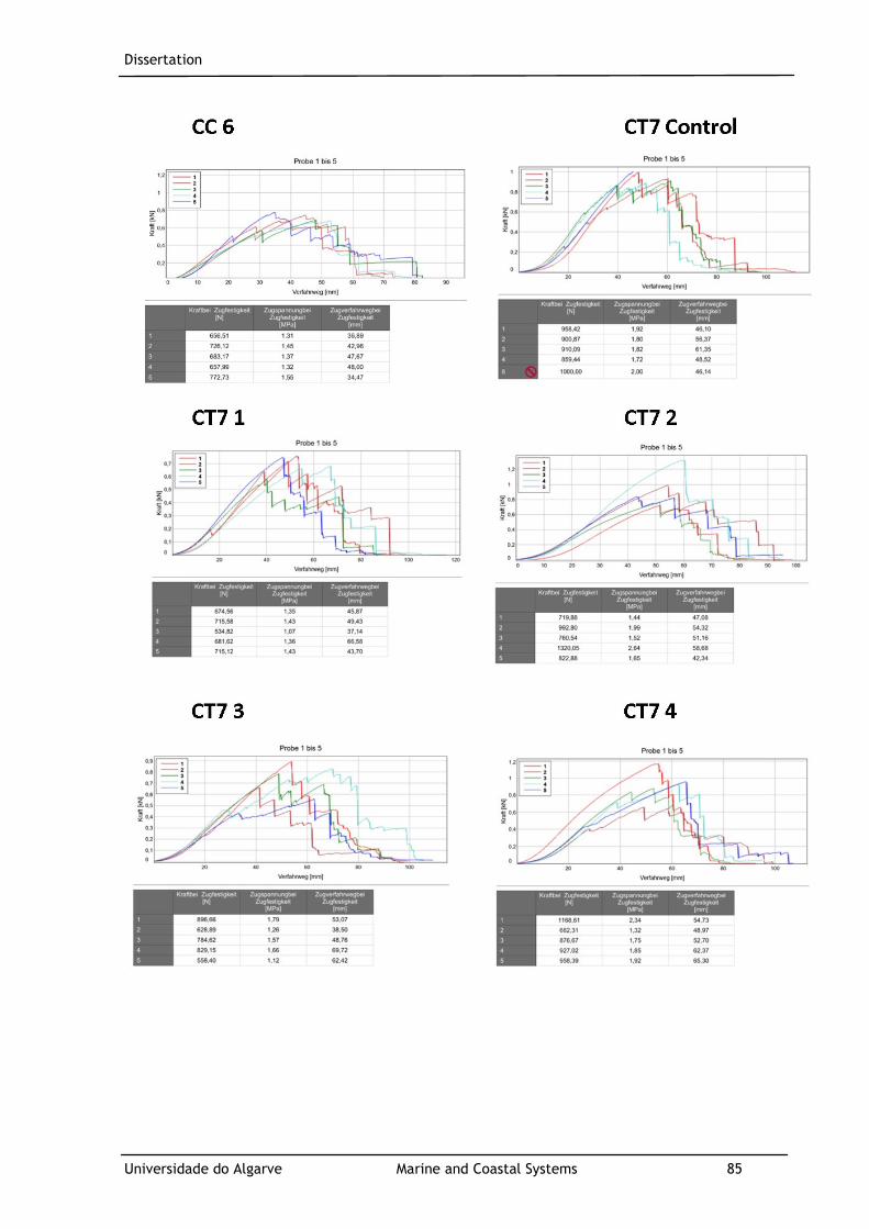
Dissertation
Universidade do Algarve Marine and Coastal Systems 85
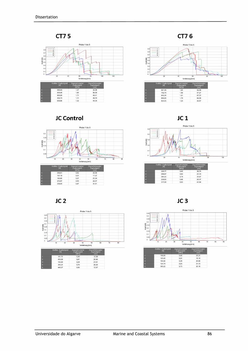
Dissertation
Universidade do Algarve Marine and Coastal Systems 86

Dissertation
Universidade do Algarve Marine and Coastal Systems 87
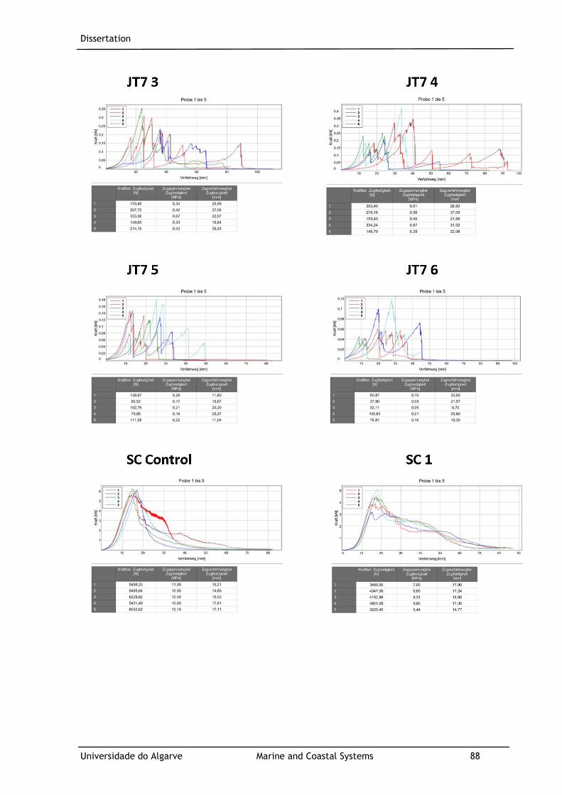
Dissertation
Universidade do Algarve Marine and Coastal Systems 88

Dissertation
Universidade do Algarve Marine and Coastal Systems 89
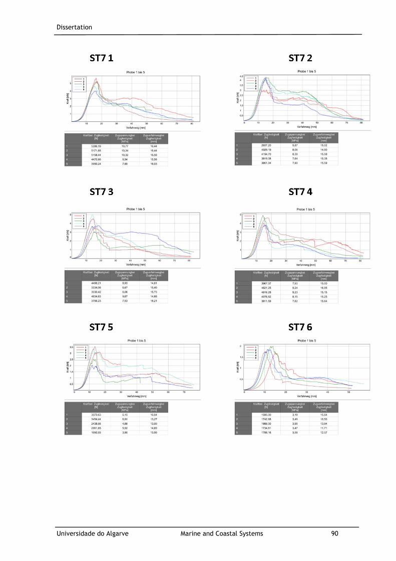
Dissertation
Universidade do Algarve Marine and Coastal Systems 90
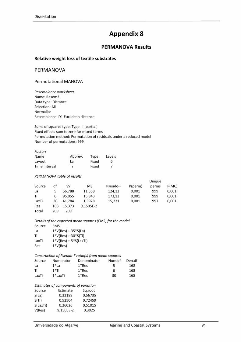
Dissertation
Universidade do Algarve Marine and Coastal Systems 91
Appendix 8
PERMANOVA Results
Relative weight loss of textile substrates
PERMANOVA
Permutational MANOVA Resemblance worksheet
Name: Resem3 Data type: Distance Selection: All Normalise Resemblance: D1 Euclidean distance Sums of squares type: Type III (partial) Fixed effects sum to zero for mixed terms Permutation method: Permutation of residuals under a reduced model Number of permutations: 999 Factors
Name Abbrev. Type Levels Layout La Fixed 6 Time Interval Ti Fixed 7 PERMANOVA table of results
Unique Source df SS MS Pseudo-F P(perm) perms P(MC) La 5 56,788 11,358 124,12 0,001 999 0,001 Ti 6 95,055 15,843 173,13 0,001 999 0,001 LaxTi 30 41,784 1,3928 15,221 0,001 997 0,001 Res 168 15,373 9,1505E-2 Total 209 209 Details of the expected mean squares (EMS) for the model
Source EMS La 1*V(Res) + 35*S(La) Ti 1*V(Res) + 30*S(Ti) LaxTi 1*V(Res) + 5*S(LaxTi) Res 1*V(Res) Construction of Pseudo-F ratio(s) from mean squares
Source Numerator Denominator Num.df Den.df La 1*La 1*Res 5 168 Ti 1*Ti 1*Res 6 168 LaxTi 1*LaxTi 1*Res 30 168 Estimates of components of variation
Source Estimate Sq.root S(La) 0,32189 0,56735 S(Ti) 0,52504 0,72459 S(LaxTi) 0,26026 0,51015 V(Res) 9,1505E-2 0,3025
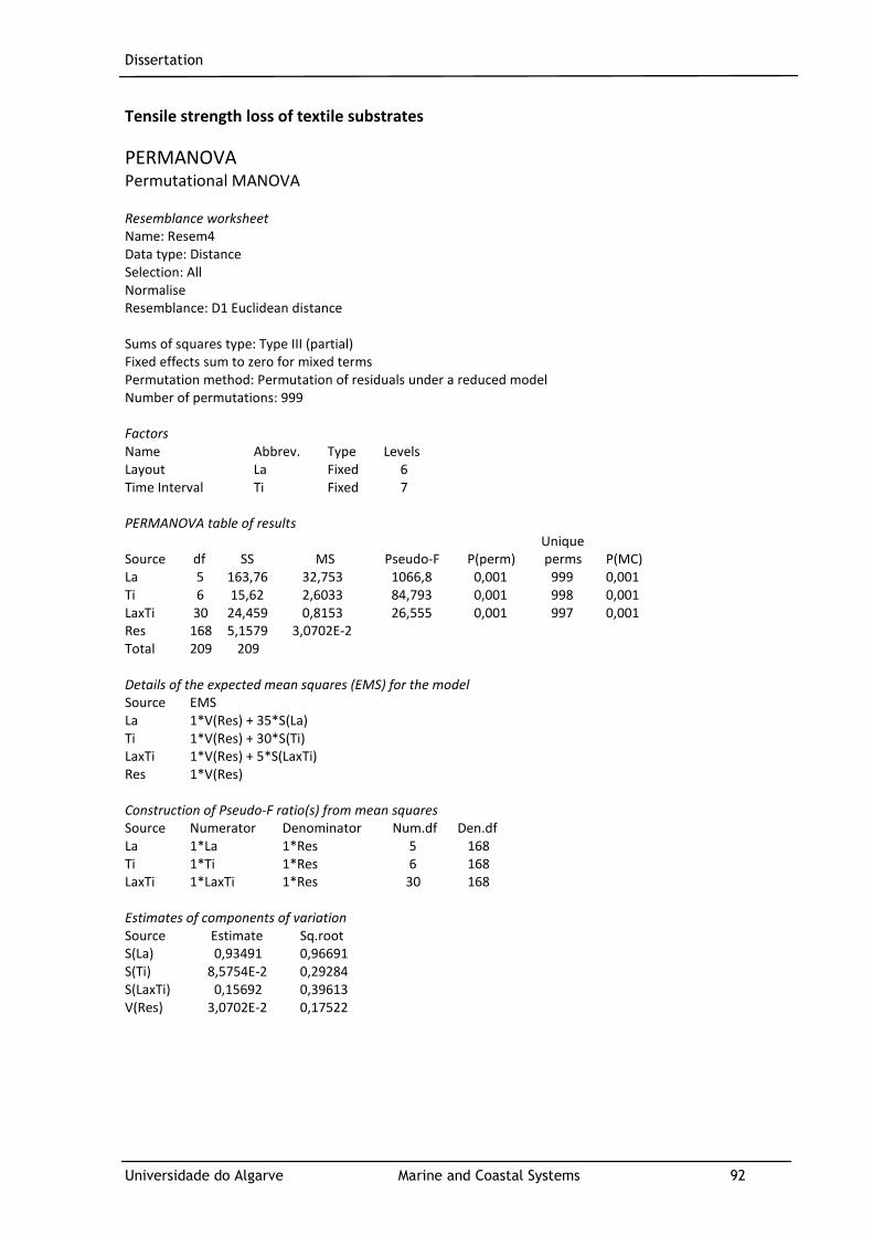
Dissertation
Universidade do Algarve Marine and Coastal Systems 92
Tensile strength loss of textile substrates
PERMANOVA Permutational MANOVA Resemblance worksheet
Name: Resem4 Data type: Distance Selection: All Normalise Resemblance: D1 Euclidean distance Sums of squares type: Type III (partial) Fixed effects sum to zero for mixed terms Permutation method: Permutation of residuals under a reduced model Number of permutations: 999 Factors
Name Abbrev. Type Levels Layout La Fixed 6 Time Interval Ti Fixed 7 PERMANOVA table of results
Unique Source df SS MS Pseudo-F P(perm) perms P(MC) La 5 163,76 32,753 1066,8 0,001 999 0,001 Ti 6 15,62 2,6033 84,793 0,001 998 0,001 LaxTi 30 24,459 0,8153 26,555 0,001 997 0,001 Res 168 5,1579 3,0702E-2 Total 209 209 Details of the expected mean squares (EMS) for the model
Source EMS La 1*V(Res) + 35*S(La) Ti 1*V(Res) + 30*S(Ti) LaxTi 1*V(Res) + 5*S(LaxTi) Res 1*V(Res) Construction of Pseudo-F ratio(s) from mean squares
Source Numerator Denominator Num.df Den.df La 1*La 1*Res 5 168 Ti 1*Ti 1*Res 6 168 LaxTi 1*LaxTi 1*Res 30 168 Estimates of components of variation
Source Estimate Sq.root S(La) 0,93491 0,96691 S(Ti) 8,5754E-2 0,29284 S(LaxTi) 0,15692 0,39613 V(Res) 3,0702E-2 0,17522
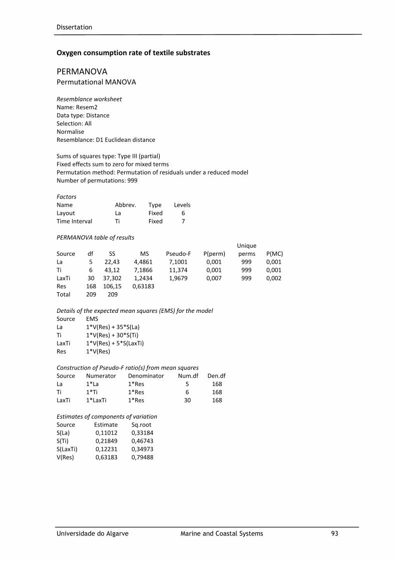
Dissertation
Universidade do Algarve Marine and Coastal Systems 93
Oxygen consumption rate of textile substrates
PERMANOVA Permutational MANOVA Resemblance worksheet
Name: Resem2 Data type: Distance Selection: All Normalise Resemblance: D1 Euclidean distance Sums of squares type: Type III (partial) Fixed effects sum to zero for mixed terms Permutation method: Permutation of residuals under a reduced model Number of permutations: 999 Factors
Name Abbrev. Type Levels Layout La Fixed 6 Time Interval Ti Fixed 7 PERMANOVA table of results
Unique Source df SS MS Pseudo-F P(perm) perms P(MC) La 5 22,43 4,4861 7,1001 0,001 999 0,001 Ti 6 43,12 7,1866 11,374 0,001 999 0,001 LaxTi 30 37,302 1,2434 1,9679 0,007 999 0,002 Res 168 106,15 0,63183 Total 209 209 Details of the expected mean squares (EMS) for the model
Source EMS La 1*V(Res) + 35*S(La) Ti 1*V(Res) + 30*S(Ti) LaxTi 1*V(Res) + 5*S(LaxTi) Res 1*V(Res) Construction of Pseudo-F ratio(s) from mean squares
Source Numerator Denominator Num.df Den.df La 1*La 1*Res 5 168 Ti 1*Ti 1*Res 6 168 LaxTi 1*LaxTi 1*Res 30 168 Estimates of components of variation
Source Estimate Sq.root S(La) 0,11012 0,33184 S(Ti) 0,21849 0,46743 S(LaxTi) 0,12231 0,34973 V(Res) 0,63183 0,79488

Dissertation
Universidade do Algarve Marine and Coastal Systems 94
PERMANOVA post-hoc results
Relative weight loss of textile substrates in factor ‘Layout’
PERMANOVA Permutational MANOVA Resemblance worksheet Name: Resem3 Data type: Distance Selection: All Normalise Resemblance: D1 Euclidean distance Sums of squares type: Type III (partial) Fixed effects sum to zero for mixed terms Permutation method: Permutation of residuals under a reduced model Number of permutations: 999 Factors Name Abbrev. Type Levels Layout La Fixed 6 Time Interval Ti Fixed 7 PAIR-WISE TESTS Term 'LaxTi' for pairs of levels of factor 'Layout' Within level '0' of factor 'Time Interval' Unique Groups t P(perm) perms P(MC) CC, CT7 Denominator is 0 CC, JC Denominator is 0 CC, JT7 Denominator is 0 CC, SC Denominator is 0 CC, ST7 Denominator is 0 CT7, JC Denominator is 0 CT7, JT7 Denominator is 0 CT7, SC Denominator is 0 CT7, ST7 Denominator is 0 JC, JT7 Denominator is 0 JC, SC Denominator is 0 JC, ST7 Denominator is 0 JT7, SC Denominator is 0 JT7, ST7 Denominator is 0 SC, ST7 Denominator is 0 Denominators Groups Denominator Den.df CC, CT7 1*Res 0 CC, JC 1*Res 0 CC, JT7 1*Res 0 CC, SC 1*Res 0 CC, ST7 1*Res 0 CT7, JC 1*Res 0 CT7, JT7 1*Res 0 CT7, SC 1*Res 0 CT7, ST7 1*Res 0 JC, JT7 1*Res 0 JC, SC 1*Res 0 JC, ST7 1*Res 0 JT7, SC 1*Res 0 JT7, ST7 1*Res 0 SC, ST7 1*Res 0 Average Distance between/within groups CC CT7 JC JT7 SC ST7 CC 0 CT7 0 0 JC 0 0 0 JT7 0 0 0 0 SC 0 0 0 0 0 ST7 0 0 0 0 0 0 Within level '1' of factor 'Time Interval' Unique Groups t P(perm) perms P(MC) CC, CT7 1,1093E-2 0,992 125 0,993 CC, JC 2,0579 0,098 126 0,084 CC, JT7 1,0594 0,307 126 0,309 CC, SC 7,3055 0,008 126 0,001 CC, ST7 10,034 0,011 126 0,001 CT7, JC 0,87997 0,435 126 0,41 CT7, JT7 0,50195 0,646 126 0,618 CT7, SC 5,3001 0,007 126 0,001 CT7, ST7 4,0018 0,027 126 0,003
Within level '3' of factor 'Time Interval' Unique Groups t P(perm) perms P(MC) CC, CT7 3,6246 0,028 126 0,009 CC, JC 7,4048 0,008 126 0,001 CC, JT7 1,6628 0,108 126 0,138 CC, SC 7,8567 0,005 126 0,001 CC, ST7 9,4296 0,008 126 0,001 CT7, JC 1,7002 0,076 126 0,131 CT7, JT7 0,11531 0,931 126 0,898 CT7, SC 5,5115 0,013 126 0,001 CT7, ST7 5,6768 0,009 126 0,001 JC, JT7 0,83884 0,507 126 0,397 JC, SC 5,1916 0,007 126 0,001 JC, ST7 5,7045 0,005 126 0,001 JT7, SC 3,9752 0,017 126 0,007 JT7, ST7 3,2973 0,038 126 0,014 SC, ST7 1,5707 0,154 125 0,156 Denominators Groups Denominator Den.df CC, CT7 1*Res 8 CC, JC 1*Res 8 CC, JT7 1*Res 8 CC, SC 1*Res 8 CC, ST7 1*Res 8 CT7, JC 1*Res 8 CT7, JT7 1*Res 8 CT7, SC 1*Res 8 CT7, ST7 1*Res 8 JC, JT7 1*Res 8 JC, SC 1*Res 8 JC, ST7 1*Res 8 JT7, SC 1*Res 8 JT7, ST7 1*Res 8 SC, ST7 1*Res 8 Average Distance between/within groups CC CT7 JC JT7 SC ST7 CC 0,1556 CT7 0,34101 0,18123 JC 0,46164 0,14011 6,4999E-2 JT7 0,32726 0,31258 0,3648 0,4226 SC 1,2224 0,88929 0,76078 0,93012 0,40211 ST7 0,95984 0,62671 0,4982 0,68297 0,35188 0,22119 Within level '4' of factor 'Time Interval' Unique Groups t P(perm) perms P(MC) CC, CT7 3,5111 0,009 126 0,009 CC, JC 3,2295 0,014 126 0,016 CC, JT7 1,5891 0,113 126 0,154 CC, SC 6,444 0,013 126 0,001 CC, ST7 8,4386 0,01 126 0,001 CT7, JC 0,25099 0,802 126 0,811 CT7, JT7 0,32844 0,808 126 0,766 CT7, SC 4,2352 0,008 126 0,004 CT7, ST7 3,9375 0,018 125 0,003 JC, JT7 0,43754 0,783 125 0,675 JC, SC 4,4015 0,007 126 0,006 JC, ST7 4,2125 0,015 126 0,002 JT7, SC 2,3136 0,063 126 0,049 JT7, ST7 1,3993 0,168 125 0,201 SC, ST7 1,7598 0,094 126 0,105 Denominators Groups Denominator Den.df CC, CT7 1*Res 8 CC, JC 1*Res 8 CC, JT7 1*Res 8 CC, SC 1*Res 8 CC, ST7 1*Res 8 CT7, JC 1*Res 8 CT7, JT7 1*Res 8 CT7, SC 1*Res 8 CT7, ST7 1*Res 8 JC, JT7 1*Res 8 JC, SC 1*Res 8 JC, ST7 1*Res 8 JT7, SC 1*Res 8 JT7, ST7 1*Res 8 SC, ST7 1*Res 8 Average Distance between/within groups CC CT7 JC JT7 SC ST7 CC 0,11415 CT7 0,33336 0,23586 JC 0,30759 0,19875 0,23502 JT7 0,51711 0,41969 0,41117 0,66835 SC 1,1564 0,82308 0,85318 0,85491 0,45916 ST7 0,8132 0,48189 0,51061 0,61762 0,40019 0,24384 Within level '5' of factor 'Time Interval' Unique Groups t P(perm) perms P(MC) CC, CT7 2,8007 0,031 126 0,023 CC, JC 10,758 0,01 126 0,001 CC, JT7 5,4802 0,011 126 0,003 CC, SC 15,712 0,01 126 0,001 CC, ST7 14,855 0,01 125 0,001 CT7, JC 2,8037 0,038 126 0,019
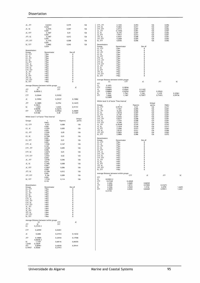
Dissertation
Universidade do Algarve Marine and Coastal Systems 95
JC, JT7 0,62321 0,575 126 0,564 JC, SC 6,0735 0,007 126 0,001 JC, ST7 6,1607 0,01 126 0,001 JT7, SC 6,2497 0,012 126 0,001 JT7, ST7 6,1735 0,008 126 0,001 SC, ST7 3,0682 0,043 126 0,024 Denominators Groups Denominator Den.df CC, CT7 1*Res 8 CC, JC 1*Res 8 CC, JT7 1*Res 8 CC, SC 1*Res 8 CC, ST7 1*Res 8 CT7, JC 1*Res 8 CT7, JT7 1*Res 8 CT7, SC 1*Res 8 CT7, ST7 1*Res 8 JC, JT7 1*Res 8 JC, SC 1*Res 8 JC, ST7 1*Res 8 JT7, SC 1*Res 8 JT7, ST7 1*Res 8 SC, ST7 1*Res 8 Average Distance between/within groups CC CT7 JC JT7 SC ST7 CC 8,8383E-2 CT7 0,22644 0,35352 JC 0,15994 0,29337 0,15082 JT7 0,14805 0,2754 0,14415 0,18231 SC 1,0451 1,0435 0,91151 0,96598 0,36274 ST7 0,59222 0,59564 0,45859 0,51306 0,48 0,13307 Within level '2' of factor 'Time Interval' Unique Groups t P(perm) perms P(MC) CC, CT7 4,414 0,008 126 0,002 CC, JC 4,3291 0,005 126 0,003 CC, JT7 2,5381 0,05 126 0,034 CC, SC 8,7598 0,01 126 0,001 CC, ST7 9,8863 0,01 126 0,001 CT7, JC 1,5382 0,167 126 0,165 CT7, JT7 3,5248 0,005 126 0,006 CT7, SC 4,4674 0,01 126 0,003 CT7, ST7 3,5431 0,02 125 0,003 JC, JT7 3,0182 0,046 126 0,016 JC, SC 6,3482 0,008 126 0,001 JC, ST7 6,2007 0,006 126 0,002 JT7, SC 8,1596 0,012 126 0,001 JT7, ST7 9,196 0,009 126 0,001 SC, ST7 1,7192 0,114 126 0,135 Denominators Groups Denominator Den.df CC, CT7 1*Res 8 CC, JC 1*Res 8 CC, JT7 1*Res 8 CC, SC 1*Res 8 CC, ST7 1*Res 8 CT7, JC 1*Res 8 CT7, JT7 1*Res 8 CT7, SC 1*Res 8 CT7, ST7 1*Res 8 JC, JT7 1*Res 8 JC, SC 1*Res 8 JC, ST7 1*Res 8 JT7, SC 1*Res 8 JT7, ST7 1*Res 8 SC, ST7 1*Res 8 Average Distance between/within groups CC CT7 JC JT7 SC ST7 CC 9,2731E-2 CT7 0,42959 0,25451 JC 0,2682 0,21914 0,14232 JT7 0,10805 0,32934 0,17558 4,6664E-2 SC 1,1107 0,68116 0,84255 1,0105 0,33039 ST7 0,85961 0,43018 0,59141 0,75937 0,30266 0,21913
CT7, JT7 2,1443 0,053 126 0,056 CT7, SC 9,3063 0,011 126 0,001 CT7, ST7 6,9714 0,007 126 0,002 JC, JT7 0,13556 0,891 126 0,907 JC, SC 10,393 0,007 126 0,002 JC, ST7 7,9917 0,013 126 0,001 JT7, SC 6,9037 0,008 126 0,001 JT7, ST7 4,2668 0,004 126 0,003 SC, ST7 4,0536 0,006 126 0,002 Denominators Groups Denominator Den.df CC, CT7 1*Res 8 CC, JC 1*Res 8 CC, JT7 1*Res 8 CC, SC 1*Res 8 CC, ST7 1*Res 8 CT7, JC 1*Res 8 CT7, JT7 1*Res 8 CT7, SC 1*Res 8 CT7, ST7 1*Res 8 JC, JT7 1*Res 8 JC, SC 1*Res 8 JC, ST7 1*Res 8 JT7, SC 1*Res 8 JT7, ST7 1*Res 8 SC, ST7 1*Res 8 Average Distance between/within groups CC CT7 JC JT7 SC ST7 CC 0,1875 CT7 0,45651 0,38266 JC 0,86802 0,43641 0,11432 JT7 0,88864 0,50702 0,24077 0,39543 SC 2,2041 1,7561 1,3361 1,3155 0,32961 ST7 1,6068 1,1587 0,73877 0,71815 0,59736 0,22809 Within level '6' of factor 'Time Interval' Unique Groups t P(perm) perms P(MC) CC, CT7 0,99174 0,35 126 0,371 CC, JC 7,1841 0,005 126 0,001 CC, JT7 16,692 0,006 126 0,001 CC, SC 7,8218 0,007 126 0,001 CC, ST7 23,187 0,007 126 0,001 CT7, JC 6,0443 0,007 126 0,001 CT7, JT7 9,8277 0,008 125 0,001 CT7, SC 7,2535 0,008 125 0,001 CT7, ST7 14,496 0,013 126 0,001 JC, JT7 0,59349 0,579 126 0,547 JC, SC 3,1018 0,018 126 0,017 JC, ST7 2,2996 0,073 125 0,063 JT7, SC 3,8735 0,011 126 0,006 JT7, ST7 5,5853 0,005 126 0,003 SC, ST7 2,0806 0,086 126 0,072 Denominators Groups Denominator Den.df CC, CT7 1*Res 8 CC, JC 1*Res 8 CC, JT7 1*Res 8 CC, SC 1*Res 8 CC, ST7 1*Res 8 CT7, JC 1*Res 8 CT7, JT7 1*Res 8 CT7, SC 1*Res 8 CT7, ST7 1*Res 8 JC, JT7 1*Res 8 JC, SC 1*Res 8 JC, ST7 1*Res 8 JT7, SC 1*Res 8 JT7, ST7 1*Res 8 SC, ST7 1*Res 8 Average Distance between/within groups CC CT7 JC JT7 SC ST7 CC 8,0381E-2 CT7 0,27349 0,42049 JC 2,2202 2,0685 0,86545 JT7 2,0248 1,8731 0,57005 0,31673 SC 4,1046 3,9529 1,9152 2,0799 1,4635 ST7 2,9839 2,8322 0,84469 0,95911 1,2221 0,31735
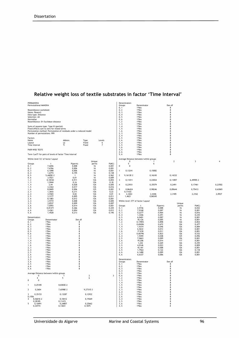
Dissertation
Universidade do Algarve Marine and Coastal Systems 96
Relative weight loss of textile substrates in factor ‘Time Interval’
PERMANOVA Permutational MANOVA Resemblance worksheet Name: Resem3 Data type: Distance Selection: All Normalise Resemblance: D1 Euclidean distance Sums of squares type: Type III (partial) Fixed effects sum to zero for mixed terms Permutation method: Permutation of residuals under a reduced model Number of permutations: 999 Factors Name Abbrev. Type Levels Layout La Fixed 6 Time Interval Ti Fixed 7 PAIR-WISE TESTS Term 'LaxTi' for pairs of levels of factor 'Time Interval' Within level 'CC' of factor 'Layout' Unique Groups t P(perm) perms P(MC) 0, 1 7,6656 0,008 16 0,001 0, 2 7,6766 0,006 16 0,001 0, 3 6,1098 0,006 16 0,001 0, 4 1,6774 0,195 16 0,138 0, 5 5,4405E-2 1 16 0,962 0, 6 3,5521 0,01 16 0,009 1, 2 0,18102 0,911 126 0,855 1, 3 1,5044 0,16 126 0,18 1, 4 3,44 0,028 126 0,005 1, 5 3,2264 0,017 126 0,016 1, 6 8,0609 0,006 125 0,001 2, 3 1,3643 0,211 126 0,22 2, 4 3,5565 0,02 126 0,01 2, 5 3,3177 0,005 126 0,011 2, 6 8,1083 0,012 126 0,001 3, 4 3,9719 0,008 126 0,005 3, 5 3,8537 0,009 126 0,007 3, 6 7,0593 0,014 126 0,001 4, 5 0,81371 0,466 126 0,435 4, 6 3,4361 0,004 126 0,012 5, 6 1,4528 0,213 126 0,196 Denominators Groups Denominator Den.df 0, 1 1*Res 8 0, 2 1*Res 8 0, 3 1*Res 8 0, 4 1*Res 8 0, 5 1*Res 8 0, 6 1*Res 8 1, 2 1*Res 8 1, 3 1*Res 8 1, 4 1*Res 8 1, 5 1*Res 8 1, 6 1*Res 8 2, 3 1*Res 8 2, 4 1*Res 8 2, 5 1*Res 8 2, 6 1*Res 8 3, 4 1*Res 8 3, 5 1*Res 8 3, 6 1*Res 8 4, 5 1*Res 8 4, 6 1*Res 8 5, 6 1*Res 8 Average Distance between/within groups 0 1 2 3 4 5 6 0 0 1 0,25185 8,8383E-2 2 0,2604 7,6598E-2 9,2731E-2 3 0,35153 0,13287 0,12932 0,1556 4 8,5601E-2 0,18412 0,19269 0,28185 0,11415 5 0,10491 0,24807 0,25662 0,34774 0,13651 0,1875
Denominators Groups Denominator Den.df 0, 1 1*Res 8 0, 2 1*Res 8 0, 3 1*Res 8 0, 4 1*Res 8 0, 5 1*Res 8 0, 6 1*Res 8 1, 2 1*Res 8 1, 3 1*Res 8 1, 4 1*Res 8 1, 5 1*Res 8 1, 6 1*Res 8 2, 3 1*Res 8 2, 4 1*Res 8 2, 5 1*Res 8 2, 6 1*Res 8 3, 4 1*Res 8 3, 5 1*Res 8 3, 6 1*Res 8 4, 5 1*Res 8 4, 6 1*Res 8 5, 6 1*Res 8 Average Distance between/within groups 0 1 2 3 4 5 6 0 0 1 0,13241 0,15082 2 9,1613E-2 0,16245 0,14232 3 0,11011 0,22834 0,11897 6,4999E-2 4 0,23931 0,35579 0,2491 0,17461 0,23502 5 0,86424 0,98246 0,85644 0,75413 0,63065 0,11432 6 2,3263 2,4446 2,3185 2,2162 2,0927 1,4621 0,86545 Within level 'JT7' of factor 'Layout' Unique Groups t P(perm) perms P(MC) 0, 1 2,5736 0,008 16 0,032 0, 2 7,9168 0,007 16 0,001 0, 3 0,2277 0,964 16 0,816 0, 4 1,3446 0,291 16 0,235 0, 5 6,0401 0,007 16 0,001 0, 6 18,126 0,005 16 0,001 1, 2 0,17893 0,898 126 0,854 1, 3 0,69496 0,672 126 0,477 1, 4 1,9374 0,046 126 0,084 1, 5 6,5632 0,012 126 0,001 1, 6 17,018 0,011 126 0,001 2, 3 0,66796 0,823 126 0,532 2, 4 1,9459 0,048 125 0,096 2, 5 7,0663 0,009 126 0,001 2, 6 19,206 0,014 117 0,001 3, 4 1,242 0,269 126 0,255 3, 5 4,0146 0,023 126 0,009 3, 6 10,181 0,008 126 0,001 4, 5 1,7564 0,122 126 0,118 4, 6 6,1488 0,009 126 0,001 5, 6 6,6337 0,006 126 0,001 Denominators Groups Denominator Den.df 0, 1 1*Res 8 0, 2 1*Res 8 0, 3 1*Res 8 0, 4 1*Res 8 0, 5 1*Res 8 0, 6 1*Res 8 1, 2 1*Res 8 1, 3 1*Res 8 1, 4 1*Res 8 1, 5 1*Res 8 1, 6 1*Res 8 2, 3 1*Res 8 2, 4 1*Res 8 2, 5 1*Res 8 2, 6 1*Res 8 3, 4 1*Res 8 3, 5 1*Res 8 3, 6 1*Res 8 4, 5 1*Res 8
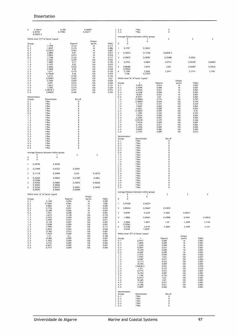
Dissertation
Universidade do Algarve Marine and Coastal Systems 97
6 0,10614 0,358 0,36655 0,45767 0,17582 0,16217 8,0381E-2 Within level 'CT7' of factor 'Layout' Unique Groups t P(perm) perms P(MC) 0, 1 1,7978 0,124 16 0,113 0, 2 1,8547 0,135 16 0,086 0, 3 0,25672 0,963 16 0,807 0, 4 3,0885 0,01 16 0,017 0, 5 3,0834 0,013 16 0,018 0, 6 1,7188 0,126 16 0,117 1, 2 2,5203 0,039 126 0,035 1, 3 1,4809 0,17 126 0,196 1, 4 3,1472 0,03 126 0,015 1, 5 3,4666 0,033 126 0,012 1, 6 2,4828 0,05 126 0,038 2, 3 1,617 0,175 126 0,154 2, 4 0,75638 0,46 126 0,479 2, 5 1,6131 0,183 126 0,154 2, 6 0,50497 0,625 126 0,63 3, 4 2,5305 0,039 126 0,036 3, 5 2,875 0,013 126 0,036 3, 6 1,6615 0,172 126 0,131 4, 5 1,0782 0,315 126 0,329 4, 6 3,3873E-2 0,971 126 0,973 5, 6 0,89625 0,405 126 0,393 Denominators Groups Denominator Den.df 0, 1 1*Res 8 0, 2 1*Res 8 0, 3 1*Res 8 0, 4 1*Res 8 0, 5 1*Res 8 0, 6 1*Res 8 1, 2 1*Res 8 1, 3 1*Res 8 1, 4 1*Res 8 1, 5 1*Res 8 1, 6 1*Res 8 2, 3 1*Res 8 2, 4 1*Res 8 2, 5 1*Res 8 2, 6 1*Res 8 3, 4 1*Res 8 3, 5 1*Res 8 3, 6 1*Res 8 4, 5 1*Res 8 4, 6 1*Res 8 5, 6 1*Res 8 Average Distance between/within groups 0 1 2 3 4 5 6 0 0 1 0,35756 0,35352 2 0,21689 0,47223 0,25451 3 0,11118 0,34994 0,243 0,18123 4 0,26369 0,54653 0,21505 0,2862 0,23586 5 0,44426 0,70803 0,34072 0,46266 0,30452 0,38266 6 0,32262 0,56323 0,29501 0,34539 0,28393 0,36642 0,42049 Within level 'JC' of factor 'Layout' Unique Groups t P(perm) perms P(MC) 0, 1 2,1109 0,054 16 0,085 0, 2 0,15041 0,841 16 0,88 0, 3 4,5864 0,01 16 0,002 0, 4 2,7736 0,051 16 0,032 0, 5 21,098 0,006 16 0,001 0, 6 7,563 0,008 16 0,001 1, 2 1,6513 0,138 126 0,135 1, 3 3,7472 0,009 126 0,007 1, 4 3,4785 0,015 126 0,011 1, 5 14,159 0,007 126 0,001 1, 6 7,8188 0,009 126 0,001 2, 3 1,7909 0,091 126 0,117 2, 4 2,2832 0,062 126 0,046 2, 5 12,962 0,013 126 0,001 2, 6 7,4329 0,009 126 0,001 3, 4 1,41 0,2 126 0,188 3, 5 15,883 0,009 126 0,001 3, 6 7,1832 0,009 126 0,001 4, 5 6,734 0,009 126 0,002 4, 6 6,5621 0,005 126 0,001 5, 6 4,7117 0,009 126 0,004
4, 6 1*Res 8 5, 6 1*Res 8 Average Distance between/within groups 0 1 2 3 4 5 6 0 0 1 0,1727 0,18231 2 0,16016 0,11526 4,6664E-2 3 0,29873 0,28381 0,25488 0,4226 4 0,4753 0,5869 0,5714 0,59378 0,66835 5 0,88486 1,0576 1,045 0,94587 0,70242 0,39543 6 2,1309 2,3036 2,2911 2,1714 1,7761 1,246 0,31673 Within level 'SC' of factor 'Layout' Unique Groups t P(perm) perms P(MC) 0, 1 5,6973 0,014 16 0,001 0, 2 6,9598 0,008 16 0,001 0, 3 6,0244 0,012 16 0,001 0, 4 6,2248 0,006 16 0,001 0, 5 18,057 0,012 16 0,001 0, 6 8,0371 0,01 16 0,001 1, 2 0,30804 0,774 126 0,787 1, 3 0,38669 0,694 126 0,704 1, 4 1,3143 0,272 126 0,229 1, 5 7,6047 0,004 126 0,001 1, 6 6,3041 0,008 126 0,001 2, 3 0,10857 0,909 126 0,92 2, 4 1,1095 0,294 126 0,291 2, 5 7,8236 0,009 126 0,001 2, 6 6,2464 0,007 126 0,002 3, 4 0,95239 0,379 126 0,366 3, 5 7,0318 0,009 126 0,001 3, 6 6,1452 0,011 126 0,001 4, 5 5,2304 0,009 126 0,002 4, 6 5,6569 0,006 126 0,002 5, 6 3,7375 0,009 126 0,013 Denominators Groups Denominator Den.df 0, 1 1*Res 8 0, 2 1*Res 8 0, 3 1*Res 8 0, 4 1*Res 8 0, 5 1*Res 8 0, 6 1*Res 8 1, 2 1*Res 8 1, 3 1*Res 8 1, 4 1*Res 8 1, 5 1*Res 8 1, 6 1*Res 8 2, 3 1*Res 8 2, 4 1*Res 8 2, 5 1*Res 8 2, 6 1*Res 8 3, 4 1*Res 8 3, 5 1*Res 8 3, 6 1*Res 8 4, 5 1*Res 8 4, 6 1*Res 8 5, 6 1*Res 8 Average Distance between/within groups 0 1 2 3 4 5 6 0 0 1 0,79328 0,36274 2 0,85034 0,29667 0,33039 3 0,8709 0,3229 0,3067 0,40211 4 1,0868 0,40361 0,37898 0,3941 0,45916 5 2,2004 1,4071 1,35 1,3295 1,1136 0,32961 6 4,2108 3,4175 3,3604 3,3399 3,124 2,0104 1,4635 Within level 'ST7' of factor 'Layout' Unique Groups t P(perm) perms P(MC) 0, 1 6,9417 0,005 16 0,001 0, 2 7,4845 0,009 16 0,001 0, 3 7,2444 0,009 16 0,001 0, 4 8,5507 0,017 16 0,001 0, 5 19,344 0,009 16 0,001 0, 6 24,687 0,009 16 0,001 1, 2 2,7572 0,036 126 0,022 1, 3 2,7557 0,03 126 0,027 1, 4 4,0387 0,017 126 0,004 1, 5 13,113 0,012 126 0,001 1, 6 20,454 0,009 126 0,001 2, 3 7,8443E-2 0,927 126 0,939 2, 4 1,221 0,237 125 0,245 2, 5 8,7115 0,012 126 0,001 2, 6 16,764 0,007 126 0,001 3, 4 1,1186 0,334 126 0,304 3, 5 8,4313 0,01 126 0,001 3, 6 16,465 0,01 126 0,001 4, 5 7,1552 0,011 125 0,001 4, 6 15,396 0,011 126 0,001 5, 6 9,9057 0,005 126 0,001 Denominators Groups Denominator Den.df 0, 1 1*Res 8 0, 2 1*Res 8 0, 3 1*Res 8 0, 4 1*Res 8 0, 5 1*Res 8
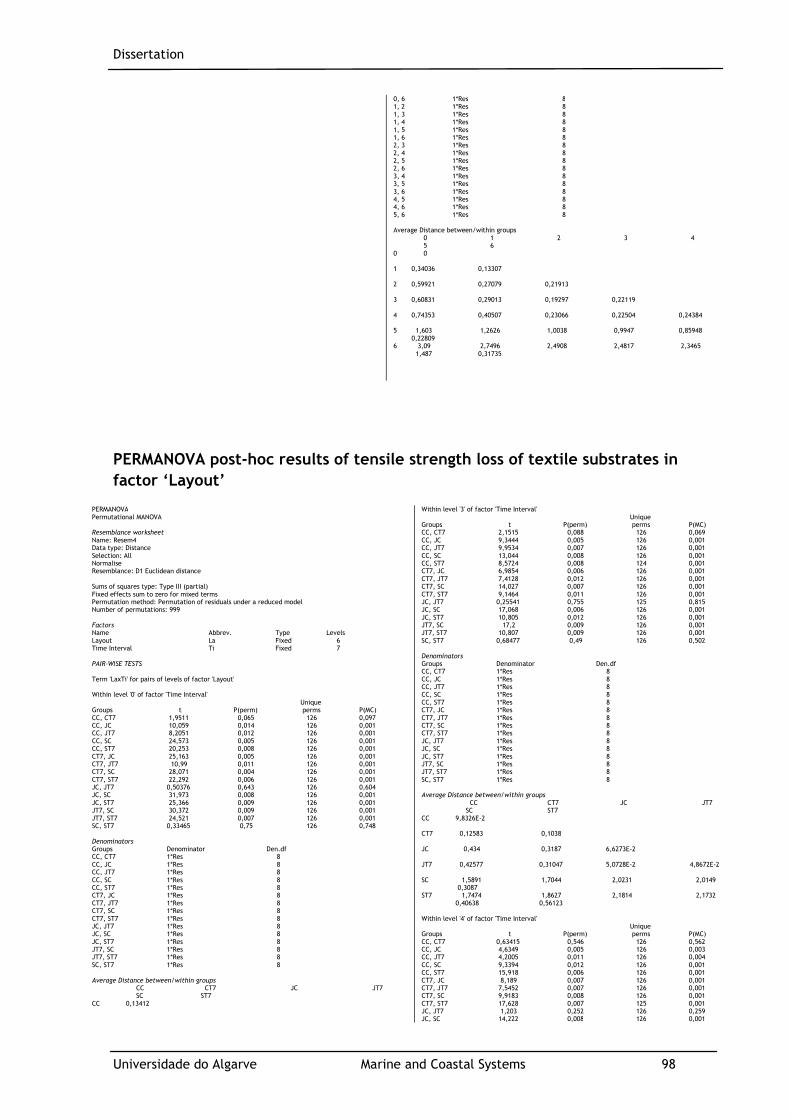
Dissertation
Universidade do Algarve Marine and Coastal Systems 98
0, 6 1*Res 8 1, 2 1*Res 8 1, 3 1*Res 8 1, 4 1*Res 8 1, 5 1*Res 8 1, 6 1*Res 8 2, 3 1*Res 8 2, 4 1*Res 8 2, 5 1*Res 8 2, 6 1*Res 8 3, 4 1*Res 8 3, 5 1*Res 8 3, 6 1*Res 8 4, 5 1*Res 8 4, 6 1*Res 8 5, 6 1*Res 8 Average Distance between/within groups 0 1 2 3 4 5 6 0 0 1 0,34036 0,13307 2 0,59921 0,27079 0,21913 3 0,60831 0,29013 0,19297 0,22119 4 0,74353 0,40507 0,23066 0,22504 0,24384 5 1,603 1,2626 1,0038 0,9947 0,85948 0,22809 6 3,09 2,7496 2,4908 2,4817 2,3465 1,487 0,31735
PERMANOVA post-hoc results of tensile strength loss of textile substrates in
factor ‘Layout’
PERMANOVA Permutational MANOVA Resemblance worksheet Name: Resem4 Data type: Distance Selection: All Normalise Resemblance: D1 Euclidean distance Sums of squares type: Type III (partial) Fixed effects sum to zero for mixed terms Permutation method: Permutation of residuals under a reduced model Number of permutations: 999 Factors Name Abbrev. Type Levels Layout La Fixed 6 Time Interval Ti Fixed 7 PAIR-WISE TESTS Term 'LaxTi' for pairs of levels of factor 'Layout' Within level '0' of factor 'Time Interval' Unique Groups t P(perm) perms P(MC) CC, CT7 1,9511 0,065 126 0,097 CC, JC 10,059 0,014 126 0,001 CC, JT7 8,2051 0,012 126 0,001 CC, SC 24,573 0,005 126 0,001 CC, ST7 20,253 0,008 126 0,001 CT7, JC 25,163 0,005 126 0,001 CT7, JT7 10,99 0,011 126 0,001 CT7, SC 28,071 0,004 126 0,001 CT7, ST7 22,292 0,006 126 0,001 JC, JT7 0,50376 0,643 126 0,604 JC, SC 31,973 0,008 126 0,001 JC, ST7 25,366 0,009 126 0,001 JT7, SC 30,372 0,009 126 0,001 JT7, ST7 24,521 0,007 126 0,001 SC, ST7 0,33465 0,75 126 0,748 Denominators Groups Denominator Den.df CC, CT7 1*Res 8 CC, JC 1*Res 8 CC, JT7 1*Res 8 CC, SC 1*Res 8 CC, ST7 1*Res 8 CT7, JC 1*Res 8 CT7, JT7 1*Res 8 CT7, SC 1*Res 8 CT7, ST7 1*Res 8 JC, JT7 1*Res 8 JC, SC 1*Res 8 JC, ST7 1*Res 8 JT7, SC 1*Res 8 JT7, ST7 1*Res 8 SC, ST7 1*Res 8 Average Distance between/within groups CC CT7 JC JT7 SC ST7 CC 0,13412
Within level '3' of factor 'Time Interval' Unique Groups t P(perm) perms P(MC) CC, CT7 2,1515 0,088 126 0,069 CC, JC 9,3444 0,005 126 0,001 CC, JT7 9,9534 0,007 126 0,001 CC, SC 13,044 0,008 126 0,001 CC, ST7 8,5724 0,008 124 0,001 CT7, JC 6,9854 0,006 126 0,001 CT7, JT7 7,4128 0,012 126 0,001 CT7, SC 14,027 0,007 126 0,001 CT7, ST7 9,1464 0,011 126 0,001 JC, JT7 0,25541 0,755 125 0,815 JC, SC 17,068 0,006 126 0,001 JC, ST7 10,805 0,012 126 0,001 JT7, SC 17,2 0,009 126 0,001 JT7, ST7 10,807 0,009 126 0,001 SC, ST7 0,68477 0,49 126 0,502 Denominators Groups Denominator Den.df CC, CT7 1*Res 8 CC, JC 1*Res 8 CC, JT7 1*Res 8 CC, SC 1*Res 8 CC, ST7 1*Res 8 CT7, JC 1*Res 8 CT7, JT7 1*Res 8 CT7, SC 1*Res 8 CT7, ST7 1*Res 8 JC, JT7 1*Res 8 JC, SC 1*Res 8 JC, ST7 1*Res 8 JT7, SC 1*Res 8 JT7, ST7 1*Res 8 SC, ST7 1*Res 8 Average Distance between/within groups CC CT7 JC JT7 SC ST7 CC 9,8326E-2 CT7 0,12583 0,1038 JC 0,434 0,3187 6,6273E-2 JT7 0,42577 0,31047 5,0728E-2 4,8672E-2 SC 1,5891 1,7044 2,0231 2,0149 0,3087 ST7 1,7474 1,8627 2,1814 2,1732 0,40638 0,56123 Within level '4' of factor 'Time Interval' Unique Groups t P(perm) perms P(MC) CC, CT7 0,63415 0,546 126 0,562 CC, JC 4,6349 0,005 126 0,003 CC, JT7 4,2005 0,011 126 0,004 CC, SC 9,3394 0,012 126 0,001 CC, ST7 15,918 0,006 126 0,001 CT7, JC 8,189 0,007 126 0,001 CT7, JT7 7,5452 0,007 126 0,001 CT7, SC 9,9183 0,008 126 0,001 CT7, ST7 17,628 0,007 125 0,001 JC, JT7 1,203 0,252 126 0,259 JC, SC 14,222 0,008 126 0,001
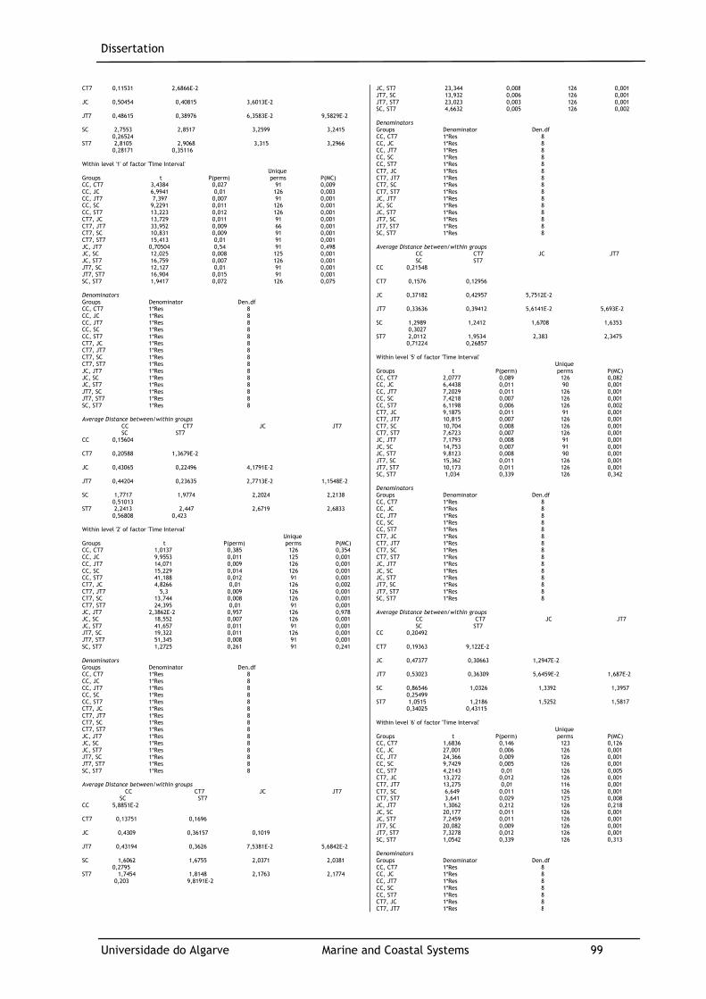
Dissertation
Universidade do Algarve Marine and Coastal Systems 99
CT7 0,11531 2,6866E-2 JC 0,50454 0,40815 3,6013E-2 JT7 0,48615 0,38976 6,3583E-2 9,5829E-2 SC 2,7553 2,8517 3,2599 3,2415 0,26524 ST7 2,8105 2,9068 3,315 3,2966 0,28171 0,35116 Within level '1' of factor 'Time Interval' Unique Groups t P(perm) perms P(MC) CC, CT7 3,4384 0,027 91 0,009 CC, JC 6,9941 0,01 126 0,003 CC, JT7 7,397 0,007 91 0,001 CC, SC 9,2291 0,011 126 0,001 CC, ST7 13,223 0,012 126 0,001 CT7, JC 13,729 0,011 91 0,001 CT7, JT7 33,952 0,009 66 0,001 CT7, SC 10,831 0,009 91 0,001 CT7, ST7 15,413 0,01 91 0,001 JC, JT7 0,70504 0,54 91 0,498 JC, SC 12,025 0,008 125 0,001 JC, ST7 16,759 0,007 126 0,001 JT7, SC 12,127 0,01 91 0,001 JT7, ST7 16,904 0,015 91 0,001 SC, ST7 1,9417 0,072 126 0,075 Denominators Groups Denominator Den.df CC, CT7 1*Res 8 CC, JC 1*Res 8 CC, JT7 1*Res 8 CC, SC 1*Res 8 CC, ST7 1*Res 8 CT7, JC 1*Res 8 CT7, JT7 1*Res 8 CT7, SC 1*Res 8 CT7, ST7 1*Res 8 JC, JT7 1*Res 8 JC, SC 1*Res 8 JC, ST7 1*Res 8 JT7, SC 1*Res 8 JT7, ST7 1*Res 8 SC, ST7 1*Res 8 Average Distance between/within groups CC CT7 JC JT7 SC ST7 CC 0,15604 CT7 0,20588 1,3679E-2 JC 0,43065 0,22496 4,1791E-2 JT7 0,44204 0,23635 2,7713E-2 1,1548E-2 SC 1,7717 1,9774 2,2024 2,2138 0,51013 ST7 2,2413 2,447 2,6719 2,6833 0,56808 0,423 Within level '2' of factor 'Time Interval' Unique Groups t P(perm) perms P(MC) CC, CT7 1,0137 0,385 126 0,354 CC, JC 9,9553 0,011 125 0,001 CC, JT7 14,071 0,009 126 0,001 CC, SC 15,229 0,014 126 0,001 CC, ST7 41,188 0,012 91 0,001 CT7, JC 4,8266 0,01 126 0,002 CT7, JT7 5,3 0,009 126 0,001 CT7, SC 13,744 0,008 126 0,001 CT7, ST7 24,395 0,01 91 0,001 JC, JT7 2,3862E-2 0,957 126 0,978 JC, SC 18,552 0,007 126 0,001 JC, ST7 41,657 0,011 91 0,001 JT7, SC 19,322 0,011 126 0,001 JT7, ST7 51,345 0,008 91 0,001 SC, ST7 1,2725 0,261 91 0,241 Denominators Groups Denominator Den.df CC, CT7 1*Res 8 CC, JC 1*Res 8 CC, JT7 1*Res 8 CC, SC 1*Res 8 CC, ST7 1*Res 8 CT7, JC 1*Res 8 CT7, JT7 1*Res 8 CT7, SC 1*Res 8 CT7, ST7 1*Res 8 JC, JT7 1*Res 8 JC, SC 1*Res 8 JC, ST7 1*Res 8 JT7, SC 1*Res 8 JT7, ST7 1*Res 8 SC, ST7 1*Res 8 Average Distance between/within groups CC CT7 JC JT7 SC ST7 CC 5,8851E-2 CT7 0,13751 0,1696 JC 0,4309 0,36157 0,1019 JT7 0,43194 0,3626 7,5381E-2 5,6842E-2 SC 1,6062 1,6755 2,0371 2,0381 0,2795 ST7 1,7454 1,8148 2,1763 2,1774 0,203 9,8191E-2
JC, ST7 23,344 0,008 126 0,001 JT7, SC 13,932 0,006 126 0,001 JT7, ST7 23,023 0,003 126 0,001 SC, ST7 4,6632 0,005 126 0,002 Denominators Groups Denominator Den.df CC, CT7 1*Res 8 CC, JC 1*Res 8 CC, JT7 1*Res 8 CC, SC 1*Res 8 CC, ST7 1*Res 8 CT7, JC 1*Res 8 CT7, JT7 1*Res 8 CT7, SC 1*Res 8 CT7, ST7 1*Res 8 JC, JT7 1*Res 8 JC, SC 1*Res 8 JC, ST7 1*Res 8 JT7, SC 1*Res 8 JT7, ST7 1*Res 8 SC, ST7 1*Res 8 Average Distance between/within groups CC CT7 JC JT7 SC ST7 CC 0,21548 CT7 0,1576 0,12956 JC 0,37182 0,42957 5,7512E-2 JT7 0,33636 0,39412 5,6141E-2 5,693E-2 SC 1,2989 1,2412 1,6708 1,6353 0,3027 ST7 2,0112 1,9534 2,383 2,3475 0,71224 0,26857 Within level '5' of factor 'Time Interval' Unique Groups t P(perm) perms P(MC) CC, CT7 2,0777 0,089 126 0,082 CC, JC 6,4438 0,011 90 0,001 CC, JT7 7,2029 0,011 126 0,001 CC, SC 7,4218 0,007 126 0,001 CC, ST7 6,1198 0,006 126 0,002 CT7, JC 9,1875 0,011 91 0,001 CT7, JT7 10,815 0,007 126 0,001 CT7, SC 10,704 0,008 126 0,001 CT7, ST7 7,6723 0,007 126 0,001 JC, JT7 7,1793 0,008 91 0,001 JC, SC 14,753 0,007 91 0,001 JC, ST7 9,8123 0,008 90 0,001 JT7, SC 15,362 0,011 126 0,001 JT7, ST7 10,173 0,011 126 0,001 SC, ST7 1,034 0,339 126 0,342 Denominators Groups Denominator Den.df CC, CT7 1*Res 8 CC, JC 1*Res 8 CC, JT7 1*Res 8 CC, SC 1*Res 8 CC, ST7 1*Res 8 CT7, JC 1*Res 8 CT7, JT7 1*Res 8 CT7, SC 1*Res 8 CT7, ST7 1*Res 8 JC, JT7 1*Res 8 JC, SC 1*Res 8 JC, ST7 1*Res 8 JT7, SC 1*Res 8 JT7, ST7 1*Res 8 SC, ST7 1*Res 8 Average Distance between/within groups CC CT7 JC JT7 SC ST7 CC 0,20492 CT7 0,19363 9,122E-2 JC 0,47377 0,30663 1,2947E-2 JT7 0,53023 0,36309 5,6459E-2 1,687E-2 SC 0,86546 1,0326 1,3392 1,3957 0,25499 ST7 1,0515 1,2186 1,5252 1,5817 0,34025 0,43115 Within level '6' of factor 'Time Interval' Unique Groups t P(perm) perms P(MC) CC, CT7 1,6836 0,146 123 0,126 CC, JC 27,001 0,006 126 0,001 CC, JT7 24,366 0,009 126 0,001 CC, SC 9,7429 0,005 126 0,001 CC, ST7 4,2143 0,01 126 0,005 CT7, JC 13,272 0,012 126 0,001 CT7, JT7 13,275 0,01 116 0,001 CT7, SC 6,649 0,011 126 0,001 CT7, ST7 3,641 0,029 125 0,008 JC, JT7 1,3062 0,212 126 0,218 JC, SC 20,177 0,011 126 0,001 JC, ST7 7,2459 0,011 126 0,001 JT7, SC 20,082 0,009 126 0,001 JT7, ST7 7,3278 0,012 126 0,001 SC, ST7 1,0542 0,339 126 0,313 Denominators Groups Denominator Den.df CC, CT7 1*Res 8 CC, JC 1*Res 8 CC, JT7 1*Res 8 CC, SC 1*Res 8 CC, ST7 1*Res 8 CT7, JC 1*Res 8 CT7, JT7 1*Res 8

Dissertation
Universidade do Algarve Marine and Coastal Systems 100
CT7, SC 1*Res 8 CT7, ST7 1*Res 8 JC, JT7 1*Res 8 JC, SC 1*Res 8 JC, ST7 1*Res 8 JT7, SC 1*Res 8 JT7, ST7 1*Res 8 SC, ST7 1*Res 8 Average Distance between/within groups CC CT7 JC JT7 SC ST7 CC 3,5442E-2 CT7 7,7012E-2 8,8127E-2 JC 0,36593 0,42377 9,3587E-3 JT7 0,37759 0,43543 1,8706E-2 2,2531E-2 SC 0,38139 0,32356 0,74732 0,75898 9,7784E-2 ST7 0,51532 0,46947 0,88125 0,89291 0,26542 0,30158
PERMANOVA post-hoc results of tensile strength loss of textile substrates in
factor ‘Time Interval’
PERMANOVA Permutational MANOVA Resemblance worksheet Name: Resem4 Data type: Distance Selection: All Normalise Resemblance: D1 Euclidean distance Sums of squares type: Type III (partial) Fixed effects sum to zero for mixed terms Permutation method: Permutation of residuals under a reduced model Number of permutations: 999 Factors Name Abbrev. Type Levels Layout La Fixed 6 Time Interval Ti Fixed 7 PAIR-WISE TESTS Term 'LaxTi' for pairs of levels of factor 'Time Interval' Within level 'CC' of factor 'Layout' Unique Groups t P(perm) perms P(MC) 0, 1 0,25733 0,789 126 0,828 0, 2 0,38151 0,746 126 0,719 0, 3 1,3431 0,244 126 0,224 0, 4 1,6438 0,15 126 0,139 0, 5 0,50452 0,651 126 0,637 0, 6 4,4276 0,006 126 0,003 1, 2 7,6551E-3 1 126 0,994 1, 3 0,89233 0,391 126 0,416 1, 4 1,3342 0,251 126 0,2 1, 5 0,26019 0,803 126 0,779 1, 6 3,318 0,028 125 0,01 2, 3 1,4237 0,173 126 0,201 2, 4 1,6154 0,138 126 0,133 2, 5 0,31513 0,745 126 0,754 2, 6 7,9707 0,01 126 0,001 3, 4 0,77631 0,467 126 0,481 3, 5 0,46694 0,609 126 0,653 3, 6 3,431 0,008 126 0,006 4, 5 0,99149 0,374 126 0,358 4, 6 0,91887 0,367 126 0,397 5, 6 2,3866 0,061 126 0,058 Denominators Groups Denominator Den.df 0, 1 1*Res 8 0, 2 1*Res 8 0, 3 1*Res 8 0, 4 1*Res 8 0, 5 1*Res 8 0, 6 1*Res 8 1, 2 1*Res 8 1, 3 1*Res 8 1, 4 1*Res 8 1, 5 1*Res 8 1, 6 1*Res 8 2, 3 1*Res 8 2, 4 1*Res 8 2, 5 1*Res 8 2, 6 1*Res 8 3, 4 1*Res 8 3, 5 1*Res 8 3, 6 1*Res 8 4, 5 1*Res 8 4, 6 1*Res 8 5, 6 1*Res 8 Average Distance between/within groups 0 1 2 3 4 5 6 0 0,13412 1 0,12172 0,15604 2 8,6961E-2 9,7388E-2 5,8851E-2
Denominators Groups Denominator Den.df 0, 1 1*Res 8 0, 2 1*Res 8 0, 3 1*Res 8 0, 4 1*Res 8 0, 5 1*Res 8 0, 6 1*Res 8 1, 2 1*Res 8 1, 3 1*Res 8 1, 4 1*Res 8 1, 5 1*Res 8 1, 6 1*Res 8 2, 3 1*Res 8 2, 4 1*Res 8 2, 5 1*Res 8 2, 6 1*Res 8 3, 4 1*Res 8 3, 5 1*Res 8 3, 6 1*Res 8 4, 5 1*Res 8 4, 6 1*Res 8 5, 6 1*Res 8 Average Distance between/within groups 0 1 2 3 4 5 6 0 9,5829E-2 1 6,607E-2 1,1548E-2 2 7,3703E-2 3,5419E-2 5,6842E-2 3 6,5873E-2 5,6196E-2 6,7287E-2 4,8672E-2 4 6,7542E-2 3,7367E-2 5,464E-2 4,9876E-2 5,693E-2 5 9,0866E-2 0,11278 0,1224 6,5804E-2 8,8146E-2 1,687E-2 6 0,11395 0,13799 0,14761 9,1019E-2 0,11336 2,7639E-2 2,2531E-2 Within level 'SC' of factor 'Layout' Unique Groups t P(perm) perms P(MC) 0, 1 4,8093 0,006 126 0,004 0, 2 8,0929 0,009 126 0,001 0, 3 8,133 0,013 126 0,001 0, 4 10,461 0,01 126 0,001 0, 5 14,243 0,012 126 0,001 0, 6 24,119 0,008 126 0,001 1, 2 0,79196 0,501 126 0,47 1, 3 1,1381 0,251 126 0,296 1, 4 2,7921 0,023 126 0,023 1, 5 4,5683 0,009 126 0,005 1, 6 8,5551 0,007 126 0,001 2, 3 0,51504 0,603 126 0,627 2, 4 2,8207 0,044 126 0,03 2, 5 5,5676 0,015 126 0,002 2, 6 13,017 0,01 126 0,001 3, 4 2,1854 0,081 126 0,071 3, 5 4,6625 0,008 126 0,002 3, 6 11,099 0,008 126 0,001 4, 5 2,2316 0,067 126 0,051 4, 6 8,1586 0,008 126 0,001 5, 6 6,7639 0,008 126 0,002 Denominators Groups Denominator Den.df 0, 1 1*Res 8 0, 2 1*Res 8 0, 3 1*Res 8 0, 4 1*Res 8 0, 5 1*Res 8 0, 6 1*Res 8 1, 2 1*Res 8 1, 3 1*Res 8 1, 4 1*Res 8 1, 5 1*Res 8 1, 6 1*Res 8 2, 3 1*Res 8 2, 4 1*Res 8
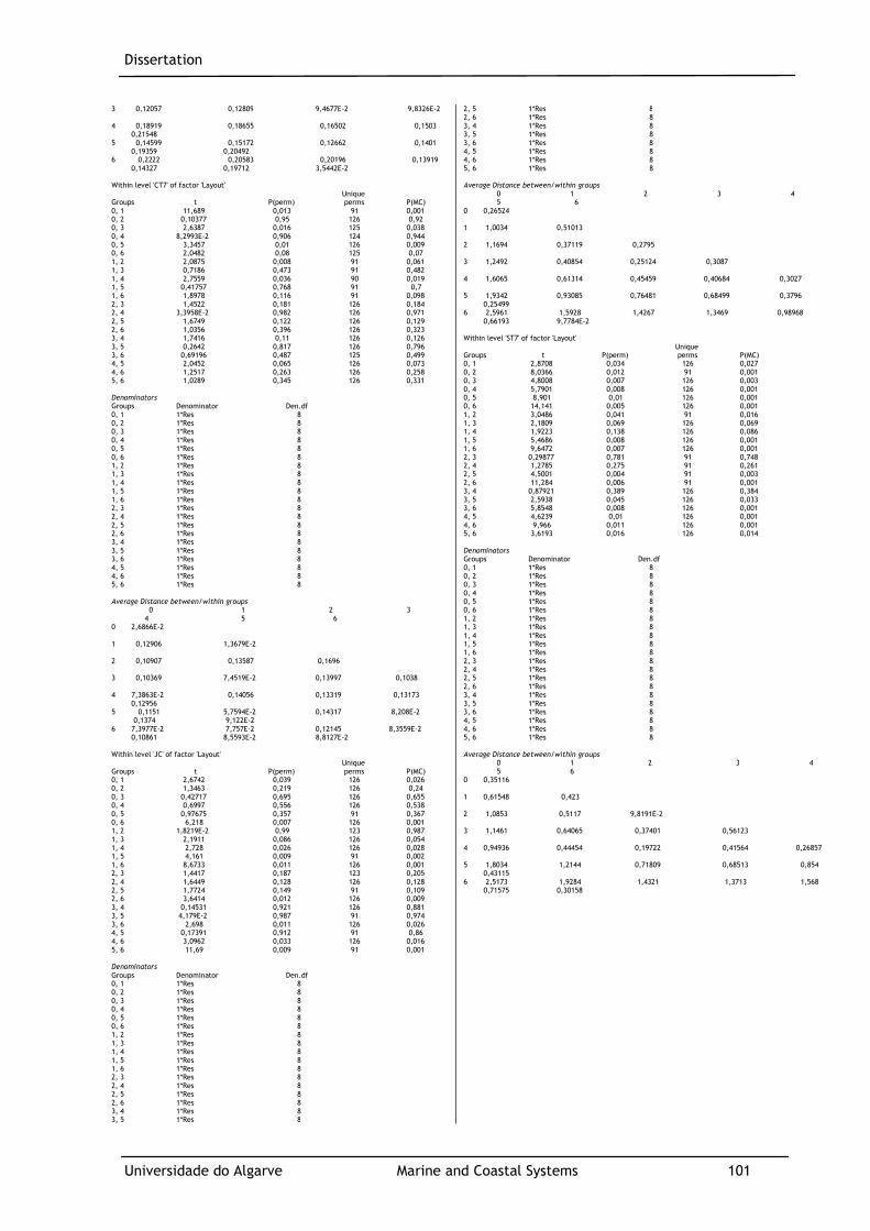
Dissertation
Universidade do Algarve Marine and Coastal Systems 101
3 0,12057 0,12809 9,4677E-2 9,8326E-2 4 0,18919 0,18655 0,16502 0,1503 0,21548 5 0,14599 0,15172 0,12662 0,1401 0,19359 0,20492 6 0,2222 0,20583 0,20196 0,13919 0,14327 0,19712 3,5442E-2 Within level 'CT7' of factor 'Layout' Unique Groups t P(perm) perms P(MC) 0, 1 11,689 0,013 91 0,001 0, 2 0,10377 0,95 126 0,92 0, 3 2,6387 0,016 125 0,038 0, 4 8,2993E-2 0,906 124 0,944 0, 5 3,3457 0,01 126 0,009 0, 6 2,0482 0,08 125 0,07 1, 2 2,0875 0,008 91 0,061 1, 3 0,7186 0,473 91 0,482 1, 4 2,7559 0,036 90 0,019 1, 5 0,41757 0,768 91 0,7 1, 6 1,8978 0,116 91 0,098 2, 3 1,4522 0,181 126 0,184 2, 4 3,3958E-2 0,982 126 0,971 2, 5 1,6749 0,122 126 0,129 2, 6 1,0356 0,396 126 0,323 3, 4 1,7416 0,11 126 0,126 3, 5 0,2642 0,817 126 0,796 3, 6 0,69196 0,487 125 0,499 4, 5 2,0452 0,065 126 0,073 4, 6 1,2517 0,263 126 0,258 5, 6 1,0289 0,345 126 0,331 Denominators Groups Denominator Den.df 0, 1 1*Res 8 0, 2 1*Res 8 0, 3 1*Res 8 0, 4 1*Res 8 0, 5 1*Res 8 0, 6 1*Res 8 1, 2 1*Res 8 1, 3 1*Res 8 1, 4 1*Res 8 1, 5 1*Res 8 1, 6 1*Res 8 2, 3 1*Res 8 2, 4 1*Res 8 2, 5 1*Res 8 2, 6 1*Res 8 3, 4 1*Res 8 3, 5 1*Res 8 3, 6 1*Res 8 4, 5 1*Res 8 4, 6 1*Res 8 5, 6 1*Res 8 Average Distance between/within groups 0 1 2 3 4 5 6 0 2,6866E-2 1 0,12906 1,3679E-2 2 0,10907 0,13587 0,1696 3 0,10369 7,4519E-2 0,13997 0,1038 4 7,3863E-2 0,14056 0,13319 0,13173 0,12956 5 0,1151 5,7594E-2 0,14317 8,208E-2 0,1374 9,122E-2 6 7,3977E-2 7,757E-2 0,12145 8,3559E-2 0,10861 8,5593E-2 8,8127E-2 Within level 'JC' of factor 'Layout' Unique Groups t P(perm) perms P(MC) 0, 1 2,6742 0,039 126 0,026 0, 2 1,3463 0,219 126 0,24 0, 3 0,42717 0,695 126 0,655 0, 4 0,6997 0,556 126 0,538 0, 5 0,97675 0,357 91 0,367 0, 6 6,218 0,007 126 0,001 1, 2 1,8219E-2 0,99 123 0,987 1, 3 2,1911 0,086 126 0,054 1, 4 2,728 0,026 126 0,028 1, 5 4,161 0,009 91 0,002 1, 6 8,6733 0,011 126 0,001 2, 3 1,4417 0,187 123 0,205 2, 4 1,6449 0,128 126 0,128 2, 5 1,7724 0,149 91 0,109 2, 6 3,6414 0,012 126 0,009 3, 4 0,14531 0,921 126 0,881 3, 5 4,179E-2 0,987 91 0,974 3, 6 2,698 0,011 126 0,026 4, 5 0,17391 0,912 91 0,86 4, 6 3,0962 0,033 126 0,016 5, 6 11,69 0,009 91 0,001 Denominators Groups Denominator Den.df 0, 1 1*Res 8 0, 2 1*Res 8 0, 3 1*Res 8 0, 4 1*Res 8 0, 5 1*Res 8 0, 6 1*Res 8 1, 2 1*Res 8 1, 3 1*Res 8 1, 4 1*Res 8 1, 5 1*Res 8 1, 6 1*Res 8 2, 3 1*Res 8 2, 4 1*Res 8 2, 5 1*Res 8 2, 6 1*Res 8 3, 4 1*Res 8 3, 5 1*Res 8
2, 5 1*Res 8 2, 6 1*Res 8 3, 4 1*Res 8 3, 5 1*Res 8 3, 6 1*Res 8 4, 5 1*Res 8 4, 6 1*Res 8 5, 6 1*Res 8 Average Distance between/within groups 0 1 2 3 4 5 6 0 0,26524 1 1,0034 0,51013 2 1,1694 0,37119 0,2795 3 1,2492 0,40854 0,25124 0,3087 4 1,6065 0,61314 0,45459 0,40684 0,3027 5 1,9342 0,93085 0,76481 0,68499 0,3796 0,25499 6 2,5961 1,5928 1,4267 1,3469 0,98968 0,66193 9,7784E-2 Within level 'ST7' of factor 'Layout' Unique Groups t P(perm) perms P(MC) 0, 1 2,8708 0,034 126 0,027 0, 2 8,0366 0,012 91 0,001 0, 3 4,8008 0,007 126 0,003 0, 4 5,7901 0,008 126 0,001 0, 5 8,901 0,01 126 0,001 0, 6 14,141 0,005 126 0,001 1, 2 3,0486 0,041 91 0,016 1, 3 2,1809 0,069 126 0,069 1, 4 1,9223 0,138 126 0,086 1, 5 5,4686 0,008 126 0,001 1, 6 9,6472 0,007 126 0,001 2, 3 0,29877 0,781 91 0,748 2, 4 1,2785 0,275 91 0,261 2, 5 4,5001 0,004 91 0,003 2, 6 11,284 0,006 91 0,001 3, 4 0,87921 0,389 126 0,384 3, 5 2,5938 0,045 126 0,033 3, 6 5,8548 0,008 126 0,001 4, 5 4,6239 0,01 126 0,001 4, 6 9,966 0,011 126 0,001 5, 6 3,6193 0,016 126 0,014 Denominators Groups Denominator Den.df 0, 1 1*Res 8 0, 2 1*Res 8 0, 3 1*Res 8 0, 4 1*Res 8 0, 5 1*Res 8 0, 6 1*Res 8 1, 2 1*Res 8 1, 3 1*Res 8 1, 4 1*Res 8 1, 5 1*Res 8 1, 6 1*Res 8 2, 3 1*Res 8 2, 4 1*Res 8 2, 5 1*Res 8 2, 6 1*Res 8 3, 4 1*Res 8 3, 5 1*Res 8 3, 6 1*Res 8 4, 5 1*Res 8 4, 6 1*Res 8 5, 6 1*Res 8 Average Distance between/within groups 0 1 2 3 4 5 6 0 0,35116 1 0,61548 0,423 2 1,0853 0,5117 9,8191E-2 3 1,1461 0,64065 0,37401 0,56123 4 0,94936 0,44454 0,19722 0,41564 0,26857 5 1,8034 1,2144 0,71809 0,68513 0,854 0,43115 6 2,5173 1,9284 1,4321 1,3713 1,568 0,71575 0,30158
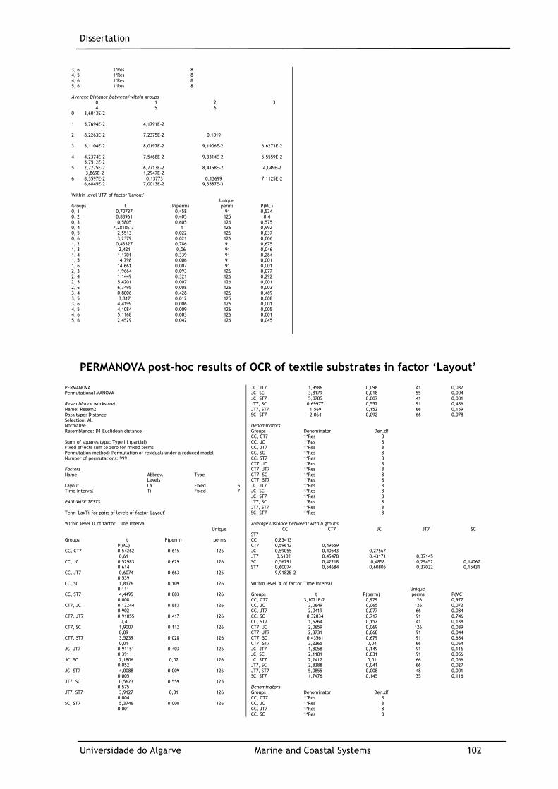
Dissertation
Universidade do Algarve Marine and Coastal Systems 102
3, 6 1*Res 8 4, 5 1*Res 8 4, 6 1*Res 8 5, 6 1*Res 8 Average Distance between/within groups 0 1 2 3 4 5 6 0 3,6013E-2 1 5,7694E-2 4,1791E-2 2 8,2263E-2 7,2375E-2 0,1019 3 5,1104E-2 8,0197E-2 9,1906E-2 6,6273E-2 4 4,2374E-2 7,5468E-2 9,3314E-2 5,5559E-2 5,7512E-2 5 2,7275E-2 6,7713E-2 8,4158E-2 4,049E-2 3,869E-2 1,2947E-2 6 8,3597E-2 0,13773 0,13699 7,1125E-2 6,6845E-2 7,0013E-2 9,3587E-3 Within level 'JT7' of factor 'Layout' Unique Groups t P(perm) perms P(MC) 0, 1 0,70737 0,458 91 0,524 0, 2 0,83961 0,405 125 0,4 0, 3 0,5805 0,605 126 0,575 0, 4 7,2818E-3 1 126 0,992 0, 5 2,5513 0,022 126 0,037 0, 6 3,2379 0,021 126 0,006 1, 2 0,43327 0,786 91 0,675 1, 3 2,421 0,06 91 0,046 1, 4 1,1701 0,339 91 0,284 1, 5 14,798 0,006 91 0,001 1, 6 14,661 0,007 91 0,001 2, 3 1,9664 0,093 126 0,077 2, 4 1,1449 0,321 126 0,292 2, 5 5,4201 0,007 126 0,001 2, 6 6,3495 0,008 126 0,003 3, 4 0,8006 0,428 126 0,469 3, 5 3,317 0,012 125 0,008 3, 6 4,4199 0,006 126 0,001 4, 5 4,1084 0,009 126 0,005 4, 6 5,1168 0,003 126 0,001 5, 6 2,4529 0,042 126 0,045
PERMANOVA post-hoc results of OCR of textile substrates in factor ‘Layout’
PERMANOVA Permutational MANOVA Resemblance worksheet Name: Resem2 Data type: Distance Selection: All Normalise Resemblance: D1 Euclidean distance Sums of squares type: Type III (partial) Fixed effects sum to zero for mixed terms Permutation method: Permutation of residuals under a reduced model Number of permutations: 999 Factors Name Abbrev. Type Levels Layout La Fixed 6 Time Interval Ti Fixed 7 PAIR-WISE TESTS Term 'LaxTi' for pairs of levels of factor 'Layout' Within level '0' of factor 'Time Interval' Unique Groups t P(perm) perms P(MC) CC, CT7 0,54262 0,615 126 0,61 CC, JC 0,52983 0,629 126 0,614 CC, JT7 0,6074 0,663 126 0,539 CC, SC 1,8176 0,109 126 0,111 CC, ST7 4,4495 0,003 126 0,008 CT7, JC 0,12244 0,883 126 0,902 CT7, JT7 0,91055 0,417 126 0,4 CT7, SC 1,9007 0,112 126 0,09 CT7, ST7 3,5239 0,028 126 0,01 JC, JT7 0,91151 0,403 126 0,391 JC, SC 2,1806 0,07 126 0,052 JC, ST7 4,0088 0,009 126 0,005 JT7, SC 0,5623 0,559 125 0,575 JT7, ST7 3,9127 0,01 126 0,004 SC, ST7 5,3746 0,008 126 0,001
JC, JT7 1,9586 0,098 41 0,087 JC, SC 3,8179 0,018 55 0,004 JC, ST7 5,0705 0,007 41 0,001 JT7, SC 0,69977 0,552 91 0,486 JT7, ST7 1,569 0,152 66 0,159 SC, ST7 2,064 0,092 66 0,078 Denominators Groups Denominator Den.df CC, CT7 1*Res 8 CC, JC 1*Res 8 CC, JT7 1*Res 8 CC, SC 1*Res 8 CC, ST7 1*Res 8 CT7, JC 1*Res 8 CT7, JT7 1*Res 8 CT7, SC 1*Res 8 CT7, ST7 1*Res 8 JC, JT7 1*Res 8 JC, SC 1*Res 8 JC, ST7 1*Res 8 JT7, SC 1*Res 8 JT7, ST7 1*Res 8 SC, ST7 1*Res 8 Average Distance between/within groups CC CT7 JC JT7 SC ST7 CC 0,83413 CT7 0,59612 0,49559 JC 0,59055 0,40543 0,27567 JT7 0,6102 0,45478 0,43171 0,37145 SC 0,56291 0,42218 0,4858 0,29452 0,14067 ST7 0,60074 0,54684 0,60805 0,37032 0,15431 9,9182E-2 Within level '4' of factor 'Time Interval' Unique Groups t P(perm) perms P(MC) CC, CT7 3,1021E-2 0,979 126 0,977 CC, JC 2,0649 0,065 126 0,072 CC, JT7 2,0419 0,077 66 0,084 CC, SC 0,32834 0,717 91 0,746 CC, ST7 1,6264 0,152 41 0,138 CT7, JC 2,0659 0,069 126 0,089 CT7, JT7 2,3731 0,068 91 0,044 CT7, SC 0,43561 0,679 91 0,684 CT7, ST7 2,2365 0,04 66 0,064 JC, JT7 1,8058 0,149 91 0,116 JC, SC 2,1101 0,031 91 0,056 JC, ST7 2,2412 0,01 66 0,056 JT7, SC 2,8388 0,041 66 0,027 JT7, ST7 5,0855 0,008 48 0,001 SC, ST7 1,7476 0,145 35 0,116 Denominators Groups Denominator Den.df CC, CT7 1*Res 8 CC, JC 1*Res 8 CC, JT7 1*Res 8 CC, SC 1*Res 8
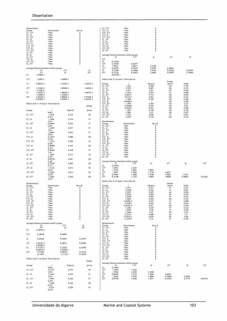
Dissertation
Universidade do Algarve Marine and Coastal Systems 103
Denominators Groups Denominator Den.df CC, CT7 1*Res 8 CC, JC 1*Res 8 CC, JT7 1*Res 8 CC, SC 1*Res 8 CC, ST7 1*Res 8 CT7, JC 1*Res 8 CT7, JT7 1*Res 8 CT7, SC 1*Res 8 CT7, ST7 1*Res 8 JC, JT7 1*Res 8 JC, SC 1*Res 8 JC, ST7 1*Res 8 JT7, SC 1*Res 8 JT7, ST7 1*Res 8 SC, ST7 1*Res 8 Average Distance between/within groups CC CT7 JC JT7 SC ST7 CC 1,0786E-2 CT7 1,295E-2 1,6989E-2 JC 9,8601E-3 1,2532E-2 1,2201E-2 JT7 1,5166E-2 1,8906E-2 1,6403E-2 2,316E-2 SC 1,3977E-2 1,9824E-2 1,6677E-2 1,7685E-2 1,3456E-2 ST7 4,2925E-2 3,8886E-2 3,9746E-2 4,8789E-2 5,4494E-2 2,4634E-2 Within level '1' of factor 'Time Interval' Unique Groups t P(perm) perms P(MC) CC, CT7 1,5342 0,122 66 0,163 CC, JC 1,3466 0,144 91 0,24 CC, JT7 0,50657 0,532 17 0,621 CC, SC 3,3209 0,017 91 0,01 CC, ST7 2,6846 0,025 91 0,034 CT7, JC 0,10472 0,886 126 0,918 CT7, JT7 1,4719 0,256 41 0,206 CT7, SC 0,99986 0,437 126 0,323 CT7, ST7 0,52404 0,748 91 0,61 JC, JT7 1,2857 0,212 56 0,237 JC, SC 0,82756 0,661 126 0,422 JC, ST7 0,37293 0,855 126 0,717 JT7, SC 3,1332 0,013 56 0,015 JT7, ST7 2,5402 0,013 56 0,035 SC, ST7 1,2045 0,305 126 0,273 Denominators Groups Denominator Den.df CC, CT7 1*Res 8 CC, JC 1*Res 8 CC, JT7 1*Res 8 CC, SC 1*Res 8 CC, ST7 1*Res 8 CT7, JC 1*Res 8 CT7, JT7 1*Res 8 CT7, SC 1*Res 8 CT7, ST7 1*Res 8 JC, JT7 1*Res 8 JC, SC 1*Res 8 JC, ST7 1*Res 8 JT7, SC 1*Res 8 JT7, ST7 1*Res 8 SC, ST7 1*Res 8 Average Distance between/within groups CC CT7 JC JT7 SC ST7 CC 4,1841E-2 CT7 0,28538 0,44857 JC 0,26665 0,36461 0,43415 JT7 3,4231E-2 0,28013 0,25989 3,0578E-2 SC 9,7137E-2 0,27255 0,24708 8,5861E-2 5,4525E-2 ST7 0,17469 0,28745 0,27318 0,16341 0,11727 0,16929 Within level '2' of factor 'Time Interval' Unique Groups t P(perm) perms P(MC) CC, CT7 0,3177 0,736 56 0,767 CC, JC 2,5433 0,074 91 0,03 CC, JT7 1,1891 0,346 91 0,264 CC, SC 1,1804 0,342 126 0,261 CC, ST7 0,524 0,559 91 0,614
CC, ST7 1*Res 8 CT7, JC 1*Res 8 CT7, JT7 1*Res 8 CT7, SC 1*Res 8 CT7, ST7 1*Res 8 JC, JT7 1*Res 8 JC, SC 1*Res 8 JC, ST7 1*Res 8 JT7, SC 1*Res 8 JT7, ST7 1*Res 8 SC, ST7 1*Res 8 Average Distance between/within groups CC CT7 JC JT7 SC ST7 CC 0,37766 CT7 0,27928 0,26277 JC 2,8931 2,8613 3,6198 JT7 0,42575 0,39319 2,6787 0,28661 SC 0,27286 0,24086 2,9169 0,44228 0,24979 ST7 0,27726 0,26453 3,0609 0,58701 0,19859 8,0435E-2 Within level '5' of factor 'Time Interval' Unique Groups t P(perm) perms P(MC) CC, CT7 1,434 0,308 126 0,187 CC, JC 1,7391 0,007 126 0,125 CC, JT7 2,817 0,01 123 0,019 CC, SC 2,1216 0,074 91 0,089 CC, ST7 0,40217 0,772 126 0,692 CT7, JC 0,53314 0,563 126 0,633 CT7, JT7 1,1386 0,259 126 0,306 CT7, SC 2,9948E-3 1 125 0,996 CT7, ST7 1,1857 0,304 126 0,25 JC, JT7 0,46688 0,643 126 0,65 JC, SC 0,59244 0,623 126 0,569 JC, ST7 1,553 0,148 126 0,156 JT7, SC 1,3081 0,23 126 0,207 JT7, ST7 2,524 0,046 91 0,041 SC, ST7 1,6379 0,134 125 0,129 Denominators Groups Denominator Den.df CC, CT7 1*Res 8 CC, JC 1*Res 8 CC, JT7 1*Res 8 CC, SC 1*Res 8 CC, ST7 1*Res 8 CT7, JC 1*Res 8 CT7, JT7 1*Res 8 CT7, SC 1*Res 8 CT7, ST7 1*Res 8 JC, JT7 1*Res 8 JC, SC 1*Res 8 JC, ST7 1*Res 8 JT7, SC 1*Res 8 JT7, ST7 1*Res 8 SC, ST7 1*Res 8 Average Distance between/within groups CC CT7 JC JT7 SC ST7 CC 0,19434 CT7 1,0501 1,6107 JC 1,4152 1,6061 1,9892 JT7 1,9072 1,7056 1,7118 1,8651 SC 0,91861 1,1883 1,3786 1,4826 1,1351 ST7 0,41348 1,1303 1,4845 1,8608 0,98601 0,61962 Within level '6' of factor 'Time Interval' Unique Groups t P(perm) perms P(MC) CC, CT7 1,2911 0,351 91 0,241 CC, JC 2,4438 0,032 91 0,051 CC, JT7 2,5537 0,025 66 0,038 CC, SC 2,8324 0,006 66 0,016 CC, ST7 2,5359 0,053 91 0,023 CT7, JC 1,0622 0,302 126 0,333 CT7, JT7 1,6845E-2 0,973 91 0,988 CT7, SC 0,25307 0,815 91 0,834 CT7, ST7 3,6415E-2 0,971 126 0,969 JC, JT7 1,2663 0,244 91 0,232 JC, SC 1,0453 0,38 91 0,338 JC, ST7 1,2446 0,27 125 0,24 JT7, SC 0,37171 0,688 66 0,7 JT7, ST7 3,1527E-2 0,954 90 0,98 SC, ST7 0,33703 0,76 91 0,756 Denominators Groups Denominator Den.df CC, CT7 1*Res 8 CC, JC 1*Res 8 CC, JT7 1*Res 8 CC, SC 1*Res 8 CC, ST7 1*Res 8 CT7, JC 1*Res 8 CT7, JT7 1*Res 8 CT7, SC 1*Res 8 CT7, ST7 1*Res 8 JC, JT7 1*Res 8 JC, SC 1*Res 8 JC, ST7 1*Res 8 JT7, SC 1*Res 8 JT7, ST7 1*Res 8 SC, ST7 1*Res 8 Average Distance between/within groups CC CT7 JC JT7 SC ST7 CC 0,33025 CT7 1,1568 1,7424 JC 1,9964 1,8345 2,1028 JT7 0,86432 1,2152 1,5484 0,8391 SC 1,0265 1,2595 1,4885 0,74965 0,9346 ST7 0,93755 1,2446 1,4971 0,74793 0,7719 0,87735

Dissertation
Universidade do Algarve Marine and Coastal Systems 104
CT7, JC 2,5361 0,057 91 0,031 CT7, JT7 1,0898 0,363 66 0,288 CT7, SC 1,0836 0,401 91 0,312 CT7, ST7 0,2779 0,732 66 0,789 JC, JT7 1,253 0,267 91 0,245 JC, SC 1,0128 0,338 126 0,336 JC, ST7 2,4174 0,047 91 0,042 JT7, SC 0,1375 0,883 91 0,903 JT7, ST7 0,95609 0,393 66 0,361 SC, ST7 0,97178 0,457 91 0,355 Denominators Groups Denominator Den.df CC, CT7 1*Res 8 CC, JC 1*Res 8 CC, JT7 1*Res 8 CC, SC 1*Res 8 CC, ST7 1*Res 8 CT7, JC 1*Res 8 CT7, JT7 1*Res 8 CT7, SC 1*Res 8 CT7, ST7 1*Res 8 JC, JT7 1*Res 8 JC, SC 1*Res 8 JC, ST7 1*Res 8 JT7, SC 1*Res 8 JT7, ST7 1*Res 8 SC, ST7 1*Res 8 Average Distance between/within groups CC CT7 JC JT7 SC ST7 CC 0,22272 CT7 0,1675 0,14539 JC 0,56145 0,53275 0,50149 JT7 0,33046 0,29355 0,47362 0,42464 SC 0,34804 0,30486 0,50056 0,38292 0,47589 ST7 0,17613 0,12214 0,51951 0,28627 0,30415 0,14316 Within level '3' of factor 'Time Interval' Unique Groups t P(perm) perms P(MC) CC, CT7 9,5433E-3 0,994 91 0,992 CC, JC 0,1764 0,898 56 0,861 CC, JT7 0,90805 0,397 91 0,376 CC, SC 1,3498 0,301 126 0,208 CC, ST7 1,7811 0,122 91 0,106 CT7, JC 0,26977 0,83 41 0,796 CT7, JT7 1,2434 0,278 41 0,254 CT7, SC 2,0538 0,061 91 0,092 CT7, ST7 2,7401 0,009 66 0,026
PERMANOVA post-hoc results of OCR of textile substrates in factor ‘Time
Interval’
PERMANOVA Permutational MANOVA Resemblance worksheet Name: Resem2 Data type: Distance Selection: All Normalise Resemblance: D1 Euclidean distance Sums of squares type: Type III (partial) Fixed effects sum to zero for mixed terms Permutation method: Permutation of residuals under a reduced model Number of permutations: 999 Factors Name Abbrev. Type Levels Layout La Fixed 6 Time Interval Ti Fixed 7 PAIR-WISE TESTS Term 'LaxTi' for pairs of levels of factor 'Time Interval' Within level 'CC' of factor 'Layout' Unique Groups t P(perm) perms P(MC) 0, 1 3,2984 0,008 91 0,012 0, 2 1,7429 0,047 126 0,113 0, 3 2,0021 0,025 126 0,091
Average Distance between/within groups 0 1 2 3 4 5 6 0 1,2201E-2 1 0,29809 0,43415 2 0,67112 0,53361 0,50149 3 0,66874 0,50211 0,35132 0,27567 4 3,0942 2,8931 2,6975 2,6633 3,6198 5 1,6956 1,494 1,2753 1,2112 2,6669 1,9892 6 2,287 2,0598 1,8148 1,8053 2,6511 1,8492 2,1028 Within level 'JT7' of factor 'Layout' Unique Groups t P(perm) perms P(MC) 0, 1 4,5752 0,009 56 0,003 0, 2 2,4025 0,044 91 0,047 0, 3 2,0815 0,04 91 0,072 0, 4 5,6318 0,007 91 0,002 0, 5 3,2622 0,007 126 0,016 0, 6 3,9849 0,011 91 0,006 1, 2 1,9175 0,076 41 0,084 1, 3 1,5698 0,139 41 0,156 1, 4 4,9312 0,014 41 0,002
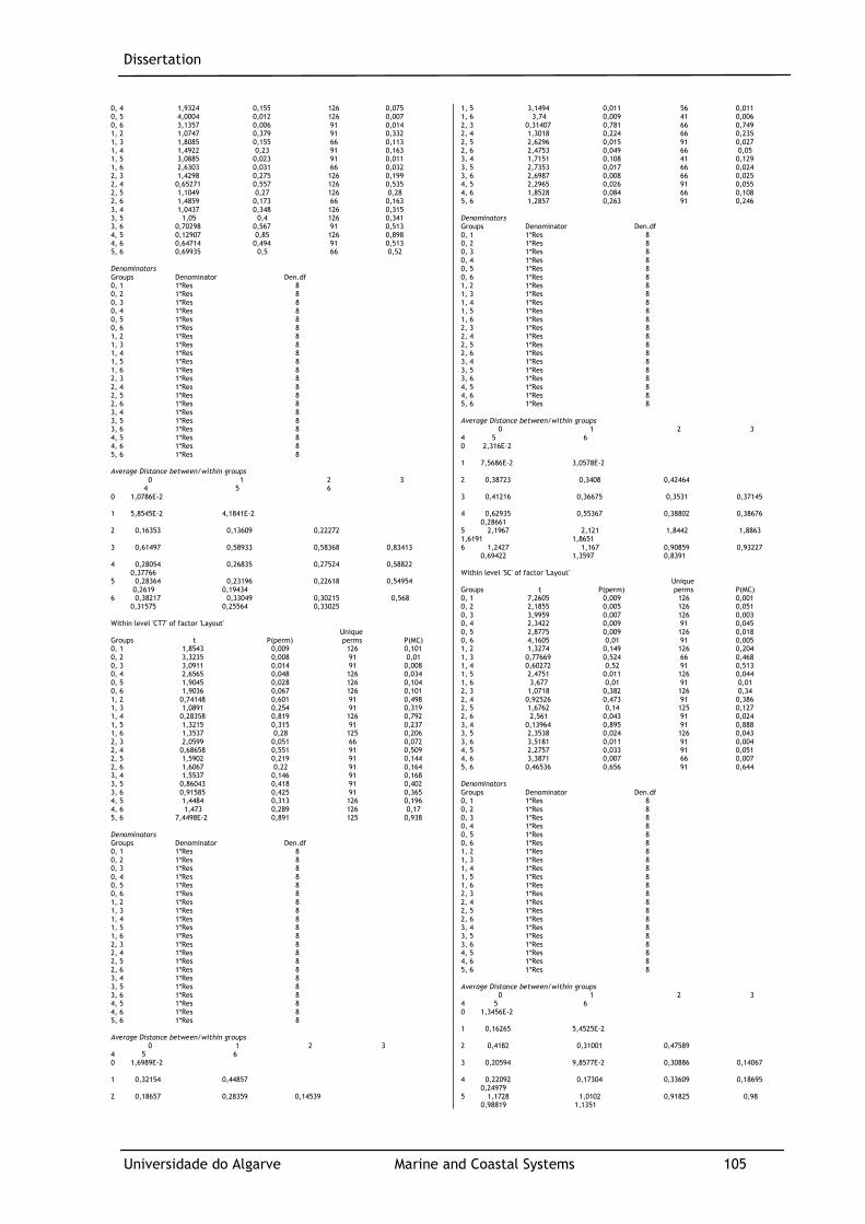
Dissertation
Universidade do Algarve Marine and Coastal Systems 105
0, 4 1,9324 0,155 126 0,075 0, 5 4,0004 0,012 126 0,007 0, 6 3,1357 0,006 91 0,014 1, 2 1,0747 0,379 91 0,332 1, 3 1,8085 0,155 66 0,113 1, 4 1,4922 0,23 91 0,163 1, 5 3,0885 0,023 91 0,011 1, 6 2,6303 0,031 66 0,032 2, 3 1,4298 0,275 126 0,199 2, 4 0,65271 0,557 126 0,535 2, 5 1,1049 0,27 126 0,28 2, 6 1,4859 0,173 66 0,163 3, 4 1,0437 0,348 126 0,315 3, 5 1,05 0,4 126 0,341 3, 6 0,70298 0,567 91 0,513 4, 5 0,12907 0,85 126 0,898 4, 6 0,64714 0,494 91 0,513 5, 6 0,69935 0,5 66 0,52 Denominators Groups Denominator Den.df 0, 1 1*Res 8 0, 2 1*Res 8 0, 3 1*Res 8 0, 4 1*Res 8 0, 5 1*Res 8 0, 6 1*Res 8 1, 2 1*Res 8 1, 3 1*Res 8 1, 4 1*Res 8 1, 5 1*Res 8 1, 6 1*Res 8 2, 3 1*Res 8 2, 4 1*Res 8 2, 5 1*Res 8 2, 6 1*Res 8 3, 4 1*Res 8 3, 5 1*Res 8 3, 6 1*Res 8 4, 5 1*Res 8 4, 6 1*Res 8 5, 6 1*Res 8 Average Distance between/within groups 0 1 2 3 4 5 6 0 1,0786E-2 1 5,8545E-2 4,1841E-2 2 0,16353 0,13609 0,22272 3 0,61497 0,58933 0,58368 0,83413 4 0,28054 0,26835 0,27524 0,58822 0,37766 5 0,28364 0,23196 0,22618 0,54954 0,2619 0,19434 6 0,38217 0,33049 0,30215 0,568 0,31575 0,25564 0,33025 Within level 'CT7' of factor 'Layout' Unique Groups t P(perm) perms P(MC) 0, 1 1,8543 0,009 126 0,101 0, 2 3,3235 0,008 91 0,01 0, 3 3,0911 0,014 91 0,008 0, 4 2,6565 0,048 126 0,034 0, 5 1,9045 0,028 126 0,104 0, 6 1,9036 0,067 126 0,101 1, 2 0,74148 0,601 91 0,498 1, 3 1,0891 0,254 91 0,319 1, 4 0,28358 0,819 126 0,792 1, 5 1,3215 0,315 91 0,237 1, 6 1,3537 0,28 125 0,206 2, 3 2,0599 0,051 66 0,072 2, 4 0,68658 0,551 91 0,509 2, 5 1,5902 0,219 91 0,144 2, 6 1,6067 0,22 91 0,164 3, 4 1,5537 0,146 91 0,168 3, 5 0,86043 0,418 91 0,402 3, 6 0,91585 0,425 91 0,365 4, 5 1,4484 0,313 126 0,196 4, 6 1,473 0,289 126 0,17 5, 6 7,4498E-2 0,891 125 0,938 Denominators Groups Denominator Den.df 0, 1 1*Res 8 0, 2 1*Res 8 0, 3 1*Res 8 0, 4 1*Res 8 0, 5 1*Res 8 0, 6 1*Res 8 1, 2 1*Res 8 1, 3 1*Res 8 1, 4 1*Res 8 1, 5 1*Res 8 1, 6 1*Res 8 2, 3 1*Res 8 2, 4 1*Res 8 2, 5 1*Res 8 2, 6 1*Res 8 3, 4 1*Res 8 3, 5 1*Res 8 3, 6 1*Res 8 4, 5 1*Res 8 4, 6 1*Res 8 5, 6 1*Res 8 Average Distance between/within groups 0 1 2 3 4 5 6 0 1,6989E-2 1 0,32154 0,44857 2 0,18657 0,28359 0,14539
1, 5 3,1494 0,011 56 0,011 1, 6 3,74 0,009 41 0,006 2, 3 0,31407 0,781 66 0,749 2, 4 1,3018 0,224 66 0,235 2, 5 2,6296 0,015 91 0,027 2, 6 2,4753 0,049 66 0,05 3, 4 1,7151 0,108 41 0,129 3, 5 2,7353 0,017 66 0,024 3, 6 2,6987 0,008 66 0,025 4, 5 2,2965 0,026 91 0,055 4, 6 1,8528 0,084 66 0,108 5, 6 1,2857 0,263 91 0,246 Denominators Groups Denominator Den.df 0, 1 1*Res 8 0, 2 1*Res 8 0, 3 1*Res 8 0, 4 1*Res 8 0, 5 1*Res 8 0, 6 1*Res 8 1, 2 1*Res 8 1, 3 1*Res 8 1, 4 1*Res 8 1, 5 1*Res 8 1, 6 1*Res 8 2, 3 1*Res 8 2, 4 1*Res 8 2, 5 1*Res 8 2, 6 1*Res 8 3, 4 1*Res 8 3, 5 1*Res 8 3, 6 1*Res 8 4, 5 1*Res 8 4, 6 1*Res 8 5, 6 1*Res 8 Average Distance between/within groups 0 1 2 3 4 5 6 0 2,316E-2 1 7,5686E-2 3,0578E-2 2 0,38723 0,3408 0,42464 3 0,41216 0,36675 0,3531 0,37145 4 0,62935 0,55367 0,38802 0,38676 0,28661 5 2,1967 2,121 1,8442 1,8863 1,6191 1,8651 6 1,2427 1,167 0,90859 0,93227 0,69422 1,3597 0,8391 Within level 'SC' of factor 'Layout' Unique Groups t P(perm) perms P(MC) 0, 1 7,2605 0,009 126 0,001 0, 2 2,1855 0,005 126 0,051 0, 3 3,9959 0,007 126 0,003 0, 4 2,3422 0,009 91 0,045 0, 5 2,8775 0,009 126 0,018 0, 6 4,1605 0,01 91 0,005 1, 2 1,3274 0,149 126 0,204 1, 3 0,77669 0,524 66 0,468 1, 4 0,60272 0,52 91 0,513 1, 5 2,4751 0,011 126 0,044 1, 6 3,677 0,01 91 0,01 2, 3 1,0718 0,382 126 0,34 2, 4 0,92526 0,473 91 0,386 2, 5 1,6762 0,14 125 0,127 2, 6 2,561 0,043 91 0,024 3, 4 0,13964 0,895 91 0,888 3, 5 2,3538 0,024 126 0,043 3, 6 3,5181 0,011 91 0,004 4, 5 2,2757 0,033 91 0,051 4, 6 3,3871 0,007 66 0,007 5, 6 0,46536 0,656 91 0,644 Denominators Groups Denominator Den.df 0, 1 1*Res 8 0, 2 1*Res 8 0, 3 1*Res 8 0, 4 1*Res 8 0, 5 1*Res 8 0, 6 1*Res 8 1, 2 1*Res 8 1, 3 1*Res 8 1, 4 1*Res 8 1, 5 1*Res 8 1, 6 1*Res 8 2, 3 1*Res 8 2, 4 1*Res 8 2, 5 1*Res 8 2, 6 1*Res 8 3, 4 1*Res 8 3, 5 1*Res 8 3, 6 1*Res 8 4, 5 1*Res 8 4, 6 1*Res 8 5, 6 1*Res 8 Average Distance between/within groups 0 1 2 3 4 5 6 0 1,3456E-2 1 0,16265 5,4525E-2 2 0,4182 0,31001 0,47589 3 0,20594 9,8577E-2 0,30886 0,14067 4 0,22092 0,17304 0,33609 0,18695 0,24979 5 1,1728 1,0102 0,91825 0,98 0,98819 1,1351

Dissertation
Universidade do Algarve Marine and Coastal Systems 106
3 0,60656 0,48166 0,44372 0,49559 4 0,28392 0,32833 0,20148 0,41294 0,26277 5 1,1567 1,0918 1,0703 1,0796 1,0752 1,6107 6 1,2823 1,2002 1,1909 1,1681 1,1787 1,3668 1,7424 Within level 'JC' of factor 'Layout' Unique Groups t P(perm) perms P(MC) 0, 1 1,6631 0,026 126 0,126 0, 2 3,6794 0,006 126 0,007 0, 3 5,8575 0,01 56 0,002 0, 4 2,2661 0,006 126 0,059 0, 5 2,0916 0,002 126 0,072 0, 6 2,9655 0,006 126 0,014 1, 2 1,4693 0,176 126 0,164 1, 3 1,7592 0,171 56 0,127 1, 4 2,0317 0,074 126 0,076 1, 5 1,6857 0,059 126 0,125 1, 6 2,5148 0,026 126 0,034 2, 3 1,103E-2 1 56 0,992 2, 4 1,759 0,128 126 0,11 2, 5 1,233 0,275 126 0,242 2, 6 2,0391 0,048 126 0,066 3, 4 1,7702 0,156 56 0,108 3, 5 1,2544 0,284 56 0,246 3, 6 2,0758 0,04 56 0,08 4, 5 0,88071 0,357 126 0,404 4, 6 0,51471 0,587 126 0,627 5, 6 0,52852 0,614 91 0,61 Denominators Groups Denominator Den.df 0, 1 1*Res 8 0, 2 1*Res 8 0, 3 1*Res 8 0, 4 1*Res 8 0, 5 1*Res 8 0, 6 1*Res 8 1, 2 1*Res 8 1, 3 1*Res 8 1, 4 1*Res 8 1, 5 1*Res 8 1, 6 1*Res 8 2, 3 1*Res 8 2, 4 1*Res 8 2, 5 1*Res 8 2, 6 1*Res 8 3, 4 1*Res 8 3, 5 1*Res 8 3, 6 1*Res 8 4, 5 1*Res 8 4, 6 1*Res 8 5, 6 1*Res 8
6 1,4202 1,2576 1,0705 1,2143 1,1993 0,89698 0,9346 Within level 'ST7' of factor 'Layout' Unique Groups t P(perm) perms P(MC) 0, 1 3,0138 0,007 126 0,021 0, 2 2,9687 0,006 91 0,026 0, 3 0,55125 0,57 91 0,565 0, 4 0,20468 0,874 66 0,844 0, 5 1,4131 0,369 126 0,197 0, 6 3,7712 0,006 126 0,006 1, 2 0,19908 0,818 66 0,851 1, 3 2,3138 0,07 91 0,067 1, 4 2,8248 0,02 66 0,017 1, 5 0,62361 0,653 126 0,538 1, 6 3,1335 0,01 125 0,016 2, 3 2,2045 0,03 66 0,053 2, 4 2,7503 0,024 30 0,021 2, 5 0,69319 0,616 91 0,528 2, 6 3,1927 0,017 91 0,014 3, 4 0,5737 0,642 48 0,584 3, 5 1,3122 0,345 91 0,253 3, 6 3,6828 0,006 91 0,008 4, 5 1,4296 0,331 66 0,195 4, 6 3,776 0,006 66 0,008 5, 6 2,1577 0,065 126 0,054 Denominators Groups Denominator Den.df 0, 1 1*Res 8 0, 2 1*Res 8 0, 3 1*Res 8 0, 4 1*Res 8 0, 5 1*Res 8 0, 6 1*Res 8 1, 2 1*Res 8 1, 3 1*Res 8 1, 4 1*Res 8 1, 5 1*Res 8 1, 6 1*Res 8 2, 3 1*Res 8 2, 4 1*Res 8 2, 5 1*Res 8 2, 6 1*Res 8 3, 4 1*Res 8 3, 5 1*Res 8 3, 6 1*Res 8 4, 5 1*Res 8 4, 6 1*Res 8 5, 6 1*Res 8 Average Distance between/within groups 0 1 2 3 4 5 6 0 2,4634E-2 1 0,18646 0,16929 2 0,16987 0,13137 0,14316 3 6,5832E-2 0,17559 0,15673 9,9182E-2 4 5,54E-2 0,19598 0,17631 8,102E-2 8,0435E-2 5 0,37383 0,40187 0,39856 0,39057 0,3914 0,61962 6 1,208 1,0335 1,0492 1,187 1,2144 1,009 0,87735
PERMADISP results of OCR
PERMDISP Distance-based test for homogeneity of multivariate dispersions Resemblance worksheet Name: Resem2 Data type: Distance Selection: All Normalise Resemblance: D1 Euclidean distance Group factor: Time Interval Number of permutations: 999 Number of groups: 7 Number of samples: 210 DEVIATIONS FROM CENTROID F: 11,384 df1: 6 df2: 203 P(perm): 0,001 PAIRWISE COMPARISONS Groups t P(perm) (0,1) 4,1072 1E-3 (0,2) 6,6218 1E-3
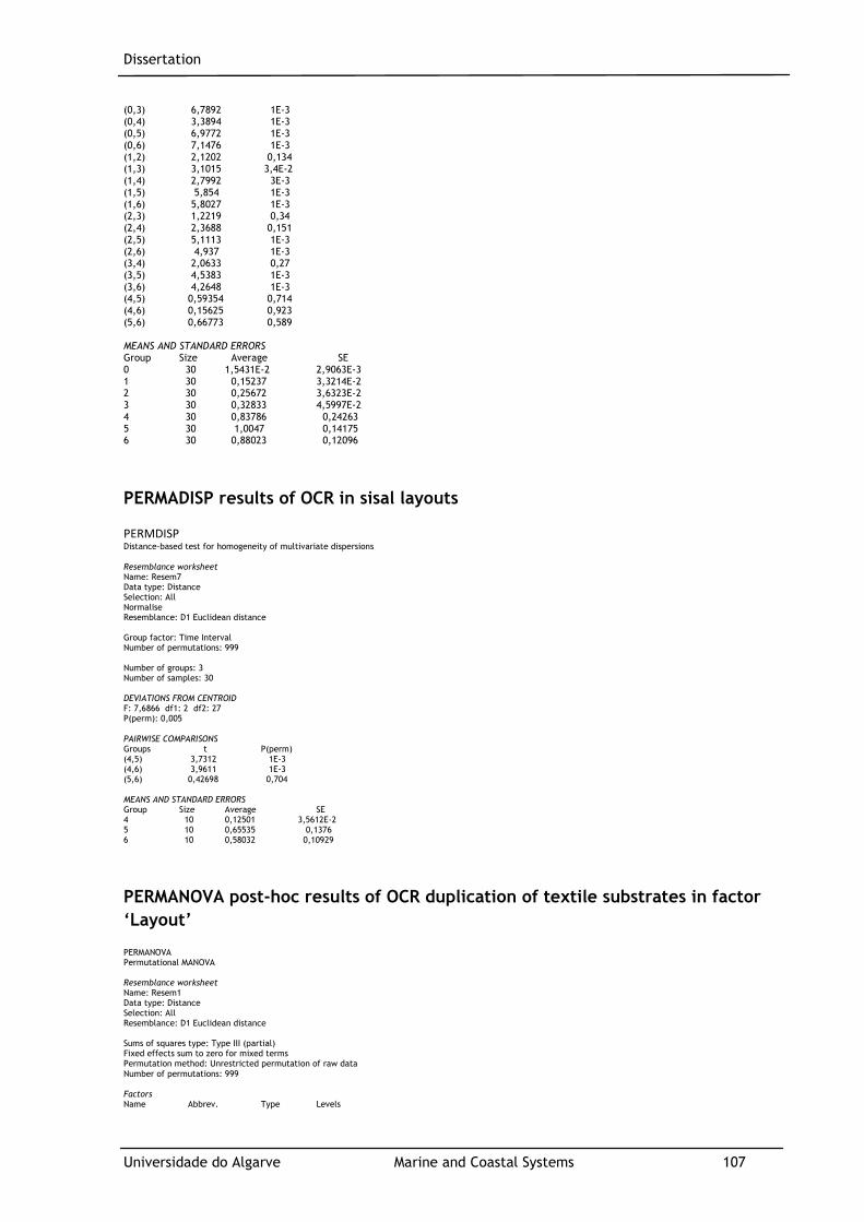
Dissertation
Universidade do Algarve Marine and Coastal Systems 107
(0,3) 6,7892 1E-3 (0,4) 3,3894 1E-3 (0,5) 6,9772 1E-3 (0,6) 7,1476 1E-3 (1,2) 2,1202 0,134 (1,3) 3,1015 3,4E-2 (1,4) 2,7992 3E-3 (1,5) 5,854 1E-3 (1,6) 5,8027 1E-3 (2,3) 1,2219 0,34 (2,4) 2,3688 0,151 (2,5) 5,1113 1E-3 (2,6) 4,937 1E-3 (3,4) 2,0633 0,27 (3,5) 4,5383 1E-3 (3,6) 4,2648 1E-3 (4,5) 0,59354 0,714 (4,6) 0,15625 0,923 (5,6) 0,66773 0,589 MEANS AND STANDARD ERRORS Group Size Average SE 0 30 1,5431E-2 2,9063E-3 1 30 0,15237 3,3214E-2 2 30 0,25672 3,6323E-2 3 30 0,32833 4,5997E-2 4 30 0,83786 0,24263 5 30 1,0047 0,14175 6 30 0,88023 0,12096
PERMADISP results of OCR in sisal layouts
PERMDISP Distance-based test for homogeneity of multivariate dispersions Resemblance worksheet Name: Resem7 Data type: Distance Selection: All Normalise Resemblance: D1 Euclidean distance Group factor: Time Interval Number of permutations: 999 Number of groups: 3 Number of samples: 30 DEVIATIONS FROM CENTROID F: 7,6866 df1: 2 df2: 27 P(perm): 0,005 PAIRWISE COMPARISONS Groups t P(perm) (4,5) 3,7312 1E-3 (4,6) 3,9611 1E-3 (5,6) 0,42698 0,704 MEANS AND STANDARD ERRORS Group Size Average SE 4 10 0,12501 3,5612E-2 5 10 0,65535 0,1376 6 10 0,58032 0,10929
PERMANOVA post-hoc results of OCR duplication of textile substrates in factor
‘Layout’
PERMANOVA Permutational MANOVA Resemblance worksheet Name: Resem1 Data type: Distance Selection: All Resemblance: D1 Euclidean distance Sums of squares type: Type III (partial) Fixed effects sum to zero for mixed terms Permutation method: Unrestricted permutation of raw data Number of permutations: 999 Factors Name Abbrev. Type Levels
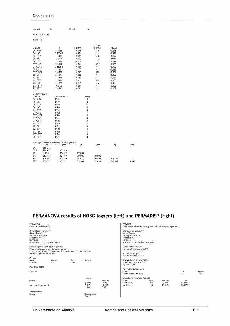
Dissertation
Universidade do Algarve Marine and Coastal Systems 108
Layout La Fixed 6 PAIR-WISE TESTS Term 'La' Unique Groups t P(perm) perms P(MC) CC, CT7 1,3028 0,196 88 0,218 CC, JC 0,76562 0,471 91 0,478 CC, JT7 1,5909 0,135 63 0,144 CC, SC 2,368 0,097 66 0,04 CC, ST7 2,9858 0,008 91 0,022 CT7, JC 2,1312 0,046 126 0,065 CT7, JT7 0,11762 0,914 91 0,927 CT7, SC 1,1811 0,37 91 0,263 CT7, ST7 2,0808 0,045 126 0,057 JC, JT7 2,5094 0,038 91 0,039 JC, SC 3,2626 0,032 91 0,011 JC, ST7 3,8486 0,01 126 0,005 JT7, SC 2,1728 0,07 66 0,053 JT7, ST7 4,342 0,011 91 0,003 SC, ST7 3,6831 0,011 91 0,008 Denominators Groups Denominator Den.df CC, CT7 1*Res 8 CC, JC 1*Res 8 CC, JT7 1*Res 8 CC, SC 1*Res 8 CC, ST7 1*Res 8 CT7, JC 1*Res 8 CT7, JT7 1*Res 8 CT7, SC 1*Res 8 CT7, ST7 1*Res 8 JC, JT7 1*Res 8 JC, SC 1*Res 8 JC, ST7 1*Res 8 JT7, SC 1*Res 8 JT7, ST7 1*Res 8 SC, ST7 1*Res 8 Average Distance between/within groups CC CT7 JC JT7 SC ST7 CC 258,33 CT7 228,65 173,68 JC 236,1 300,82 275,88 JT7 217,43 124,07 300,86 78,806 SC 244,01 118,95 345,22 76,809 40,144 ST7 285,72 135,71 392,68 126,94 56,812 13,649
PERMANOVA results of HOBO loggers (left) and PERMADISP (right)
PERMANOVA Permutational MANOVA Resemblance worksheet Name: Resem2 Data type: Distance Selection: All Normalise Resemblance: D1 Euclidean distance Sums of squares type: Type III (partial) Fixed effects sum to zero for mixed terms Permutation method: Permutation of residuals under a reduced model Number of permutations: 999 Factors Name Abbrev. Type Levels location lo Fixed 2 PAIR-WISE TESTS Term 'lo' Unique Groups t P(perm) perms P(MC) south west, north east 7,8272 0,001 996 0,001 Denominators Groups Denominator Den.df
PERMDISP Distance-based test for homogeneity of multivariate dispersions Resemblance worksheet Name: Resem2 Data type: Distance Selection: All Normalise Resemblance: D1 Euclidean distance Group factor: location Number of permutations: 999 Number of groups: 2 Number of samples: 255 DEVIATIONS FROM CENTROID F: 296,94 df1: 1 df2: 253 P(perm): 0,001 PAIRWISE COMPARISONS Groups t P(perm) (south west,north east) 17,232 1E-3 MEANS AND STANDARD ERRORS Group Size Average SE south west 165 1,0188 2,5213E-2 north east 90 0,34749 2,5377E-2
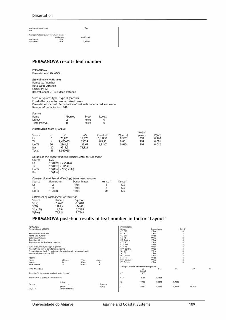
Dissertation
Universidade do Algarve Marine and Coastal Systems 109
south west, north east 1*Res 253 Average Distance between/within groups south west north east south west 1,1704 north east 1,1816 0,48012
PERMANOVA results leaf number
PERMANOVA Permutational MANOVA Resemblance worksheet Name: leaf number Data type: Distance Selection: All Resemblance: D1 Euclidean distance Sums of squares type: Type III (partial) Fixed effects sum to zero for mixed terms Permutation method: Permutation of residuals under a reduced model Number of permutations: 999 Factors Name Abbrev. Type Levels Layout La Fixed 6 Time Interval Ti Fixed 5 PERMANOVA table of results Unique Source df SS MS Pseudo-F P(perm) perms P(MC) La 5 75,873 15,175 0,19753 0,957 999 0,968 Ti 4 1,4256E5 35639 463,92 0,001 999 0,001 LaxTi 20 2941,8 147,09 1,9147 0,015 999 0,012 Res 120 9218,5 76,821 Total 149 1,5479E5 Details of the expected mean squares (EMS) for the model Source EMS La 1*V(Res) + 25*S(La) Ti 1*V(Res) + 30*S(Ti) LaxTi 1*V(Res) + 5*S(LaxTi) Res 1*V(Res) Construction of Pseudo-F ratio(s) from mean squares Source Numerator Denominator Num.df Den.df La 1*La 1*Res 5 120 Ti 1*Ti 1*Res 4 120 LaxTi 1*LaxTi 1*Res 20 120 Estimates of components of variation Source Estimate Sq.root S(La) -2,4659 -1,5703 S(Ti) 1185,4 34,43 S(LaxTi) 14,054 3,7488 V(Res) 76,821 8,7648
PERMANOVA post-hoc results of leaf number in factor ‘Layout’
PERMANOVA Permutational MANOVA Resemblance worksheet Name: leaf number Data type: Distance Selection: All Resemblance: D1 Euclidean distance Sums of squares type: Type III (partial) Fixed effects sum to zero for mixed terms Permutation method: Permutation of residuals under a reduced model Number of permutations: 999 Factors Name Abbrev. Type Levels Layout La Fixed 6 Time Interval Ti Fixed 5 PAIR-WISE TESTS Term 'LaxTi' for pairs of levels of factor 'Layout' Within level '0' of factor 'Time Interval' Unique Groups t P(perm) perms P(MC) CC, CT7 Denominator is 0
Denominators Groups Denominator Den.df CC, CT7 1*Res 8 CC, SC 1*Res 8 CC, ST7 1*Res 8 CC, FT 1*Res 8 CC, Control 1*Res 8 CT7, SC 1*Res 8 CT7, ST7 1*Res 8 CT7, FT 1*Res 8 CT7, Control 1*Res 8 SC, ST7 1*Res 8 SC, FT 1*Res 8 SC, Control 1*Res 8 ST7, FT 1*Res 8 ST7, Control 1*Res 8 FT, Control 1*Res 8 Average Distance between/within groups CC CT7 SC ST7 FT Control CC 12,039 CT7 8,9255 5,2536 SC 9,1908 7,6191 8,7989 ST7 10,847 8,3396 9,6701 12,574
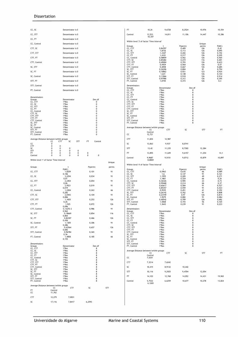
Dissertation
Universidade do Algarve Marine and Coastal Systems 110
CC, SC Denominator is 0 CC, ST7 Denominator is 0 CC, FT Denominator is 0 CC, Control Denominator is 0 CT7, SC Denominator is 0 CT7, ST7 Denominator is 0 CT7, FT Denominator is 0 CT7, Control Denominator is 0 SC, ST7 Denominator is 0 SC, FT Denominator is 0 SC, Control Denominator is 0 ST7, FT Denominator is 0 ST7, Control Denominator is 0 FT, Control Denominator is 0 Denominators Groups Denominator Den.df CC, CT7 1*Res 0 CC, SC 1*Res 0 CC, ST7 1*Res 0 CC, FT 1*Res 0 CC, Control 1*Res 0 CT7, SC 1*Res 0 CT7, ST7 1*Res 0 CT7, FT 1*Res 0 CT7, Control 1*Res 0 SC, ST7 1*Res 0 SC, FT 1*Res 0 SC, Control 1*Res 0 ST7, FT 1*Res 0 ST7, Control 1*Res 0 FT, Control 1*Res 0 Average Distance between/within groups CC CT7 SC ST7 FT Control CC 0 CT7 0 0 SC 0 0 0 ST7 0 0 0 0 FT 0 0 0 0 0 Control 0 0 0 0 0 0 Within level '1' of factor 'Time Interval' Unique Groups t P(perm) perms P(MC) CC, CT7 1,8259 0,101 91 0,106 CC, SC 3,2294 0,034 91 0,01 CC, ST7 2,2454 0,054 91 0,06 CC, FT 2,9521 0,019 91 0,019 CC, Control 1,2204 0,263 66 0,282 CT7, SC 2,0443 0,104 91 0,084 CT7, ST7 1,1835 0,253 126 0,26 CT7, FT 1,925 0,072 126 0,096 CT7, Control 5,1327E-2 0,986 91 0,962 SC, ST7 0,18669 0,854 116 0,865 SC, FT 0,82307 0,466 126 0,436 SC, Control 1,1305 0,306 91 0,286 ST7, FT 0,43564 0,657 126 0,682 ST7, Control 0,96784 0,365 91 0,36 FT, Control 1,4858 0,185 66 0,193 Denominators Groups Denominator Den.df CC, CT7 1*Res 8 CC, SC 1*Res 8 CC, ST7 1*Res 8 CC, FT 1*Res 8 CC, Control 1*Res 8 CT7, SC 1*Res 8 CT7, ST7 1*Res 8 CT7, FT 1*Res 8 CT7, Control 1*Res 8 SC, ST7 1*Res 8 SC, FT 1*Res 8 SC, Control 1*Res 8 ST7, FT 1*Res 8 ST7, Control 1*Res 8 FT, Control 1*Res 8 Average Distance between/within groups CC CT7 SC ST7 FT Control CC 11,762 CT7 12,279 7,0031 SC 17,116 7,8417 6,2593
FT 10,26 9,6728 8,2524 10,976 10,354 Control 13,523 14,811 11,106 14,447 10,386 10,347 Within level '3' of factor 'Time Interval' Unique Groups t P(perm) perms P(MC) CC, CT7 0,84707 0,409 126 0,42 CC, SC 1,8726 0,113 126 0,095 CC, ST7 1,3347 0,202 126 0,192 CC, FT 1,4101 0,217 126 0,205 CC, Control 0,58859 0,562 126 0,565 CT7, SC 0,85482 0,419 116 0,401 CT7, ST7 0,49004 0,703 126 0,623 CT7, FT 0,5929 0,564 126 0,57 CT7, Control 0,4058 0,667 126 0,685 SC, ST7 0,26206 0,804 81 0,794 SC, FT 0,10862 0,921 123 0,925 SC, Control 1,641 0,148 126 0,144 ST7, FT 0,11866 0,918 126 0,914 ST7, Control 0,97986 0,312 126 0,395 FT, Control 1,0745 0,315 126 0,3 Denominators Groups Denominator Den.df CC, CT7 1*Res 8 CC, SC 1*Res 8 CC, ST7 1*Res 8 CC, FT 1*Res 8 CC, Control 1*Res 8 CT7, SC 1*Res 8 CT7, ST7 1*Res 8 CT7, FT 1*Res 8 CT7, Control 1*Res 8 SC, ST7 1*Res 8 SC, FT 1*Res 8 SC, Control 1*Res 8 ST7, FT 1*Res 8 ST7, Control 1*Res 8 FT, Control 1*Res 8 Average Distance between/within groups CC CT7 SC ST7 FT Control CC 12,721 CT7 11,835 12,987 SC 13,063 9,937 8,0741 ST7 13,42 11,235 8,7302 12,284 FT 13,855 11,649 9,6157 11,254 14,1 Control 9,9687 9,5151 9,0712 10,879 10,897 8,8069 Within level '4' of factor 'Time Interval' Unique Groups t P(perm) perms P(MC) CC, CT7 0,5963 0,635 66 0,589 CC, SC 1,6 0,147 91 0,161 CC, ST7 1,1955 0,285 49 0,271 CC, FT 1,1861 0,324 66 0,26 CC, Control 0,36326 0,905 23 0,73 CT7, SC 0,99468 0,214 66 0,37 CT7, ST7 0,65617 0,584 91 0,527 CT7, FT 0,85357 0,559 91 0,423 CT7, Control 0,9535 0,451 41 0,352 SC, ST7 0,26142 0,762 91 0,808 SC, FT 0,23749 0,97 126 0,814 SC, Control 1,9579 0,082 91 0,084 ST7, FT 0,40542 0,709 126 0,682 ST7, Control 1,5068 0,193 56 0,165 FT, Control 1,3643 0,239 91 0,223 Denominators Groups Denominator Den.df CC, CT7 1*Res 8 CC, SC 1*Res 8 CC, ST7 1*Res 8 CC, FT 1*Res 8 CC, Control 1*Res 8 CT7, SC 1*Res 8 CT7, ST7 1*Res 8 CT7, FT 1*Res 8 CT7, Control 1*Res 8 SC, ST7 1*Res 8 SC, FT 1*Res 8 SC, Control 1*Res 8 ST7, FT 1*Res 8 ST7, Control 1*Res 8 FT, Control 1*Res 8 Average Distance between/within groups CC CT7 SC ST7 FT Control CC 7,5251 CT7 7,3214 7,6242 SC 10,415 8,9132 10,442 ST7 10,116 9,2925 9,4704 12,054 FT 14,103 12,768 14,052 14,431 19,965 Control 5,7532 6,6259 10,677 10,278 13,824 6,1265

Dissertation
Universidade do Algarve Marine and Coastal Systems 111
ST7 19,846 14,025 12,562 16,854 FT 22,311 13,5 10,366 14,523 15,462 Control 14,754 10,423 11,789 16,064 16,098 16,151 Within level '2' of factor 'Time Interval' Unique Groups t P(perm) perms P(MC) CC, CT7 0,59016 0,573 91 0,589 CC, SC 0,55071 0,606 126 0,632 CC, ST7 0,16006 0,838 66 0,867 CC, FT 0,90469 0,358 66 0,385 CC, Control 1,7879 0,1 91 0,102 CT7, SC 1,5591 0,134 66 0,158 CT7, ST7 0,36085 0,807 66 0,728 CT7, FT 1,8934 0,097 66 0,093 CT7, Control 2,9822 0,043 91 0,016 SC, ST7 0,71231 0,502 91 0,51 SC, FT 0,46035 0,59 91 0,66 SC, Control 1,5034 0,176 126 0,186 ST7, FT 1,0459 0,291 66 0,304 ST7, Control 1,898 0,09 91 0,087 FT, Control 0,98842 0,375 91 0,364
PERMANOVA post-hoc results of leaf number in factor ‘Time Interval’
PERMANOVA Permutational MANOVA Resemblance worksheet Name: leaf number Data type: Distance Selection: All Resemblance: D1 Euclidean distance Sums of squares type: Type III (partial) Fixed effects sum to zero for mixed terms Permutation method: Permutation of residuals under a reduced model Number of permutations: 999 Factors Name Abbrev. Type Levels Layout La Fixed 6 Time Interval Ti Fixed 5 PAIR-WISE TESTS Term 'LaxTi' for pairs of levels of factor 'Time Interval' Within level 'CC' of factor 'Layout' Unique Groups t P(perm) perms P(MC) 0, 1 5,1835 0,011 12 0,002 0, 2 12,89 0,011 16 0,001 0, 3 16,307 0,011 16 0,001 0, 4 33,724 0,004 12 0,001 1, 2 5,2959 0,011 91 0,001 1, 3 8,1732 0,009 91 0,001 1, 4 13,308 0,012 66 0,001 2, 3 3,0818 0,026 116 0,014 2, 4 7,1322 0,01 81 0,001 3, 4 3,1712 0,01 71 0,015 Denominators Groups Denominator Den.df 0, 1 1*Res 8 0, 2 1*Res 8 0, 3 1*Res 8 0, 4 1*Res 8 1, 2 1*Res 8 1, 3 1*Res 8 1, 4 1*Res 8 2, 3 1*Res 8 2, 4 1*Res 8 3, 4 1*Res 8 Average Distance between/within groups 0 1 2 3 4 0 0 1 23,476 11,762 2 56,997 33,522 12,039 3 76,924 53,448 20,956 12,721 4 94,314 70,839 37,317 17,391 7,5251 Within level 'CT7' of factor 'Layout' Unique Groups t P(perm) perms P(MC)
Within level 'ST7' of factor 'Layout' Unique Groups t P(perm) perms P(MC) 0, 1 6,441 0,007 16 0,002 0, 2 12,394 0,01 12 0,001 0, 3 14,472 0,007 16 0,001 0, 4 19,597 0,01 16 0,001 1, 2 2,1511 0,067 91 0,063 1, 3 3,4121 0,007 126 0,012 1, 4 6,0269 0,007 126 0,001 2, 3 1,5082 0,202 91 0,16 2, 4 4,6188 0,011 91 0,002 3, 4 3,0697 0,017 116 0,017 Denominators Groups Denominator Den.df 0, 1 1*Res 8 0, 2 1*Res 8 0, 3 1*Res 8 0, 4 1*Res 8 1, 2 1*Res 8 1, 3 1*Res 8 1, 4 1*Res 8 2, 3 1*Res 8 2, 4 1*Res 8 3, 4 1*Res 8 Average Distance between/within groups 0 1 2 3 4 0 0 1 41,024 16,854 2 58,028 18,752 12,574 3 68,035 27,011 13,019 12,284 4 87,99 46,966 29,962 21,181 12,054 Within level 'FT' of factor 'Layout' Unique Groups t P(perm) perms P(MC) 0, 1 7,9983 0,007 16 0,001 0, 2 13,665 0,008 12 0,001 0, 3 13,414 0,008 16 0,001 0, 4 10,548 0,011 16 0,001 1, 2 1,039 0,338 66 0,328 1, 3 2,9974 0,025 126 0,013 1, 4 4,0568 0,027 126 0,004 2, 3 2,4661 0,05 91 0,041 2, 4 3,681 0,017 91 0,004 3, 4 1,8084 0,119 123 0,107 Denominators Groups Denominator Den.df 0, 1 1*Res 8 0, 2 1*Res 8 0, 3 1*Res 8 0, 4 1*Res 8 1, 2 1*Res 8 1, 3 1*Res 8 1, 4 1*Res 8 2, 3 1*Res 8 2, 4 1*Res 8 3, 4 1*Res 8
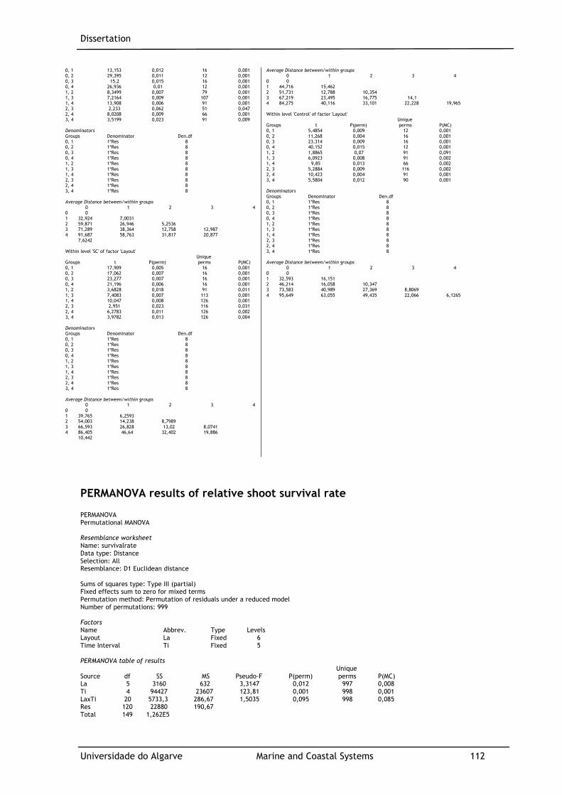
Dissertation
Universidade do Algarve Marine and Coastal Systems 112
0, 1 13,153 0,012 16 0,001 0, 2 29,395 0,011 12 0,001 0, 3 15,2 0,015 16 0,001 0, 4 26,936 0,01 12 0,001 1, 2 8,3499 0,007 79 0,001 1, 3 7,2164 0,009 107 0,001 1, 4 13,908 0,006 91 0,001 2, 3 2,233 0,062 51 0,047 2, 4 8,0208 0,009 66 0,001 3, 4 3,5199 0,023 91 0,009 Denominators Groups Denominator Den.df 0, 1 1*Res 8 0, 2 1*Res 8 0, 3 1*Res 8 0, 4 1*Res 8 1, 2 1*Res 8 1, 3 1*Res 8 1, 4 1*Res 8 2, 3 1*Res 8 2, 4 1*Res 8 3, 4 1*Res 8 Average Distance between/within groups 0 1 2 3 4 0 0 1 32,924 7,0031 2 59,871 26,946 5,2536 3 71,289 38,364 12,758 12,987 4 91,687 58,763 31,817 20,877 7,6242 Within level 'SC' of factor 'Layout' Unique Groups t P(perm) perms P(MC) 0, 1 17,909 0,005 16 0,001 0, 2 17,062 0,007 16 0,001 0, 3 23,277 0,007 16 0,001 0, 4 21,196 0,006 16 0,001 1, 2 3,6828 0,018 91 0,011 1, 3 7,4083 0,007 113 0,001 1, 4 10,047 0,008 126 0,001 2, 3 2,951 0,023 116 0,031 2, 4 6,2783 0,011 126 0,002 3, 4 3,9782 0,013 126 0,004 Denominators Groups Denominator Den.df 0, 1 1*Res 8 0, 2 1*Res 8 0, 3 1*Res 8 0, 4 1*Res 8 1, 2 1*Res 8 1, 3 1*Res 8 1, 4 1*Res 8 2, 3 1*Res 8 2, 4 1*Res 8 3, 4 1*Res 8 Average Distance between/within groups 0 1 2 3 4 0 0 1 39,765 6,2593 2 54,003 14,238 8,7989 3 66,593 26,828 13,02 8,0741 4 86,405 46,64 32,402 19,886 10,442
Average Distance between/within groups 0 1 2 3 4 0 0 1 44,716 15,462 2 51,731 12,788 10,354 3 67,219 23,495 16,775 14,1 4 84,275 40,116 33,101 22,228 19,965 Within level 'Control' of factor 'Layout' Unique Groups t P(perm) perms P(MC) 0, 1 5,4854 0,009 12 0,001 0, 2 11,268 0,004 16 0,001 0, 3 23,314 0,009 16 0,001 0, 4 40,152 0,015 12 0,001 1, 2 1,8865 0,07 91 0,091 1, 3 6,0923 0,008 91 0,002 1, 4 9,85 0,013 66 0,002 2, 3 5,2884 0,009 116 0,002 2, 4 10,423 0,004 91 0,001 3, 4 5,5804 0,012 90 0,001 Denominators Groups Denominator Den.df 0, 1 1*Res 8 0, 2 1*Res 8 0, 3 1*Res 8 0, 4 1*Res 8 1, 2 1*Res 8 1, 3 1*Res 8 1, 4 1*Res 8 2, 3 1*Res 8 2, 4 1*Res 8 3, 4 1*Res 8 Average Distance between/within groups 0 1 2 3 4 0 0 1 32,593 16,151 2 46,214 16,058 10,347 3 73,583 40,989 27,369 8,8069 4 95,649 63,055 49,435 22,066 6,1265
PERMANOVA results of relative shoot survival rate
PERMANOVA Permutational MANOVA Resemblance worksheet Name: survivalrate Data type: Distance Selection: All Resemblance: D1 Euclidean distance Sums of squares type: Type III (partial) Fixed effects sum to zero for mixed terms Permutation method: Permutation of residuals under a reduced model Number of permutations: 999 Factors Name Abbrev. Type Levels Layout La Fixed 6 Time Interval Ti Fixed 5 PERMANOVA table of results Unique Source df SS MS Pseudo-F P(perm) perms P(MC) La 5 3160 632 3,3147 0,012 997 0,008 Ti 4 94427 23607 123,81 0,001 998 0,001 LaxTi 20 5733,3 286,67 1,5035 0,095 998 0,085 Res 120 22880 190,67 Total 149 1,262E5

Dissertation
Universidade do Algarve Marine and Coastal Systems 113
Details of the expected mean squares (EMS) for the model Source EMS La 1*V(Res) + 25*S(La) Ti 1*V(Res) + 30*S(Ti) LaxTi 1*V(Res) + 5*S(LaxTi) Res 1*V(Res) Construction of Pseudo-F ratio(s) from mean squares Source Numerator Denominator Num.df Den.df La 1*La 1*Res 5 120 Ti 1*Ti 1*Res 4 120 LaxTi 1*LaxTi 1*Res 20 120 Estimates of components of variation Source Estimate Sq.root S(La) 17,653 4,2016 S(Ti) 780,53 27,938 S(LaxTi) 19,2 4,3818 V(Res) 190,67 13,808
PERMANOVA post-hoc results of relative survival rate in factor ‘Layout’
PERMANOVA Permutational MANOVA Resemblance worksheet Name: survivalrate Data type: Distance Selection: All Resemblance: D1 Euclidean distance Sums of squares type: Type III (partial) Fixed effects sum to zero for mixed terms Permutation method: Permutation of residuals under a reduced model Number of permutations: 999 Factors Name Abbrev. Type Levels Layout La Fixed 6 Time Interval Ti Fixed 5 PAIR-WISE TESTS Term 'LaxTi' for pairs of levels of factor 'Layout' Within level '0' of factor 'Time Interval' Unique Groups t P(perm) perms P(MC) CC, CT7 Denominator is 0 CC, SC Denominator is 0 CC, ST7 Denominator is 0 CC, FT Denominator is 0 CC, Control Denominator is 0 CT7, SC Denominator is 0 CT7, ST7 Denominator is 0 CT7, FT Denominator is 0 CT7, Control Denominator is 0 SC, ST7 Denominator is 0 SC, FT Denominator is 0 SC, Control Denominator is 0 ST7, FT Denominator is 0 ST7, Control Denominator is 0 FT, Control Denominator is 0 Denominators Groups Denominator Den.df CC, CT7 1*Res 0 CC, SC 1*Res 0 CC, ST7 1*Res 0 CC, FT 1*Res 0 CC, Control 1*Res 0 CT7, SC 1*Res 0 CT7, ST7 1*Res 0 CT7, FT 1*Res 0 CT7, Control 1*Res 0 SC, ST7 1*Res 0 SC, FT 1*Res 0 SC, Control 1*Res 0 ST7, FT 1*Res 0 ST7, Control 1*Res 0 FT, Control 1*Res 0 Average Distance between/within groups CC CT7 SC ST7 FT Control CC 0 CT7 0 0 SC 0 0 0
Within level '2' of factor 'Time Interval' Unique Groups t P(perm) perms P(MC) CC, CT7 1,2649 0,526 3 0,24 CC, SC 1 1 1 0,35 CC, ST7 6,2336E-9 1 2 1 CC, FT 1 1 1 0,334 CC, Control 1 1 1 0,381 CT7, SC 2,4495 0,159 2 0,037 CT7, ST7 1,2649 0,506 3 0,24 CT7, FT 2,4495 0,2 2 0,044 CT7, Control 2,4495 0,159 2 0,036 SC, ST7 1 1 1 0,334 SC, FT Denominator is 0 SC, Control Denominator is 0 ST7, FT 1 1 1 0,333 ST7, Control 1 1 1 0,321 FT, Control Denominator is 0 Denominators Groups Denominator Den.df CC, CT7 1*Res 8 CC, SC 1*Res 8 CC, ST7 1*Res 8 CC, FT 1*Res 8 CC, Control 1*Res 8 CT7, SC 1*Res 8 CT7, ST7 1*Res 8 CT7, FT 1*Res 8 CT7, Control 1*Res 8 SC, ST7 1*Res 8 SC, FT 1*Res 0 SC, Control 1*Res 0 ST7, FT 1*Res 8 ST7, Control 1*Res 8 FT, Control 1*Res 0 Average Distance between/within groups CC CT7 SC ST7 FT Control CC 8 CT7 11,2 12 SC 4 12 0 ST7 6,4 11,2 4 8 FT 4 12 0 4 0 Control 4 12 0 4 0 0 Within level '3' of factor 'Time Interval' Unique Groups t P(perm) perms P(MC) CC, CT7 0,35355 1 4 0,773 CC, SC 4,4272 0,024 4 0,003 CC, ST7 2,132 0,153 4 0,062 CC, FT 1,1767 0,441 4 0,285 CC, Control 0,63246 0,741 5 0,523 CT7, SC 2,1909 0,132 5 0,062 CT7, ST7 1,2344 0,378 5 0,249 CT7, FT 0,58977 0,777 5 0,575 CT7, Control 0,2582 1 5 0,815 SC, ST7 0,89443 0,73 3 0,398 SC, FT 1,633 0,282 4 0,132 SC, Control 1,6222 0,272 4 0,135 ST7, FT 0,66667 0,78 5 0,537 ST7, Control 0,84853 0,598 5 0,414 FT, Control 0,27217 1 5 0,79
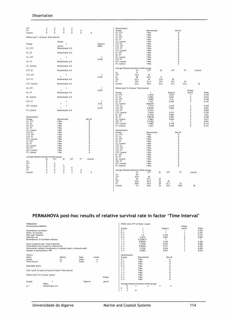
Dissertation
Universidade do Algarve Marine and Coastal Systems 114
ST7 0 0 0 0 FT 0 0 0 0 0 Control 0 0 0 0 0 0 Within level '1' of factor 'Time Interval' Unique Groups t P(perm) perms P(MC) CC, CT7 Denominator is 0 CC, SC Denominator is 0 CC, ST7 1 1 1 0,328 CC, FT Denominator is 0 CC, Control Denominator is 0 CT7, SC Denominator is 0 CT7, ST7 1 1 1 0,342 CT7, FT Denominator is 0 CT7, Control Denominator is 0 SC, ST7 1 1 1 0,355 SC, FT Denominator is 0 SC, Control Denominator is 0 ST7, FT 1 1 1 0,35 ST7, Control 1 1 1 0,315 FT, Control Denominator is 0 Denominators Groups Denominator Den.df CC, CT7 1*Res 0 CC, SC 1*Res 0 CC, ST7 1*Res 8 CC, FT 1*Res 0 CC, Control 1*Res 0 CT7, SC 1*Res 0 CT7, ST7 1*Res 8 CT7, FT 1*Res 0 CT7, Control 1*Res 0 SC, ST7 1*Res 8 SC, FT 1*Res 0 SC, Control 1*Res 0 ST7, FT 1*Res 8 ST7, Control 1*Res 8 FT, Control 1*Res 0 Average Distance between/within groups CC CT7 SC ST7 FT Control CC 0 CT7 0 0 SC 0 0 0 ST7 4 4 4 8 FT 0 0 0 4 0 Control 0 0 0 4 0 0
Denominators Groups Denominator Den.df CC, CT7 1*Res 8 CC, SC 1*Res 8 CC, ST7 1*Res 8 CC, FT 1*Res 8 CC, Control 1*Res 8 CT7, SC 1*Res 8 CT7, ST7 1*Res 8 CT7, FT 1*Res 8 CT7, Control 1*Res 8 SC, ST7 1*Res 8 SC, FT 1*Res 8 SC, Control 1*Res 8 ST7, FT 1*Res 8 ST7, Control 1*Res 8 FT, Control 1*Res 8 Average Distance between/within groups CC CT7 SC ST7 FT Control CC 12 CT7 18,4 28 SC 28 25,6 8 ST7 23,2 24 12,8 20 FT 18,4 22,4 19,2 19,2 24 Control 22,4 24,8 23,2 23,2 23,2 32 Within level '4' of factor 'Time Interval' Unique Groups t P(perm) perms P(MC) CC, CT7 1,4434 0,294 4 0,184 CC, SC 3,2863 0,041 5 0,013 CC, ST7 1,8383 0,16 6 0,109 CC, FT 1,633 0,246 5 0,145 CC, Control Negative CT7, SC 1,1314 0,418 5 0,299 CT7, ST7 0,45291 0,843 6 0,651 CT7, FT 0,2325 1 5 0,845 CT7, Control 1,4434 0,314 4 0,183 SC, ST7 0,5164 0,846 5 0,62 SC, FT 0,80178 0,581 5 0,449 SC, Control 3,2863 0,024 5 0,011 ST7, FT 0,21822 1 6 0,821 ST7, Control 1,8383 0,178 6 0,112 FT, Control 1,633 0,209 5 0,141 Denominators Groups Denominator Den.df CC, CT7 1*Res 8 CC, SC 1*Res 8 CC, ST7 1*Res 8 CC, FT 1*Res 8 CC, Control 1*Res 8 CT7, SC 1*Res 8 CT7, ST7 1*Res 8 CT7, FT 1*Res 8 CT7, Control 1*Res 8 SC, ST7 1*Res 8 SC, FT 1*Res 8 SC, Control 1*Res 8 ST7, FT 1*Res 8 ST7, Control 1*Res 8 FT, Control 1*Res 8 Average Distance between/within groups CC CT7 SC ST7 FT Control CC 20 CT7 24,8 28 SC 36 27,2 20 ST7 34,4 30,4 24 36 FT 28,8 24,8 28 31,2 32 Control 16 24,8 36 34,4 28,8 20
PERMANOVA post-hoc results of relative survival rate in factor ‘Time Interval’
PERMANOVA Permutational MANOVA Resemblance worksheet Name: survivalrate Data type: Distance Selection: All Resemblance: D1 Euclidean distance Sums of squares type: Type III (partial) Fixed effects sum to zero for mixed terms Permutation method: Permutation of residuals under a reduced model Number of permutations: 999 Factors Name Abbrev. Type Levels Layout La Fixed 6 Time Interval Ti Fixed 5 PAIR-WISE TESTS Term 'LaxTi' for pairs of levels of factor 'Time Interval' Within level 'CC' of factor 'Layout' Unique Groups t P(perm) perms P(MC) 0, 1 Denominator is 0
Within level 'ST7' of factor 'Layout' Unique Groups t P(perm) perms P(MC) 0, 1 1 1 1 0,325 0, 2 1 1 1 0,341 0, 3 1,5 0,434 2 0,167 0, 4 4,2212 0,007 8 0,004 1, 2 6,2336E-9 1 2 1 1, 3 0,89443 0,742 3 0,428 1, 4 3,7528 0,015 7 0,006 2, 3 0,89443 0,731 3 0,394 2, 4 3,7528 0,016 7 0,005 3, 4 2,8402 0,037 7 0,034 Denominators Groups Denominator Den.df 0, 1 1*Res 8 0, 2 1*Res 8 0, 3 1*Res 8 0, 4 1*Res 8 1, 2 1*Res 8 1, 3 1*Res 8 1, 4 1*Res 8 2, 3 1*Res 8 2, 4 1*Res 8 3, 4 1*Res 8 Average Distance between/within groups 0 1 2 3 4 0 0 1 4 8
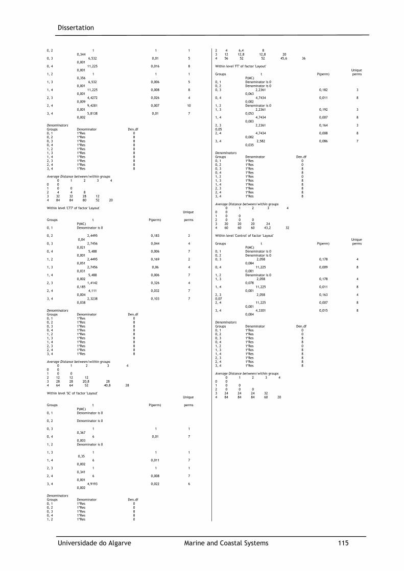
Dissertation
Universidade do Algarve Marine and Coastal Systems 115
0, 2 1 1 1 0,344 0, 3 6,532 0,01 5 0,001 0, 4 11,225 0,016 8 0,001 1, 2 1 1 1 0,356 1, 3 6,532 0,006 5 0,001 1, 4 11,225 0,008 8 0,001 2, 3 4,4272 0,026 4 0,009 2, 4 9,4281 0,007 10 0,001 3, 4 5,8138 0,01 7 0,002 Denominators Groups Denominator Den.df 0, 1 1*Res 0 0, 2 1*Res 8 0, 3 1*Res 8 0, 4 1*Res 8 1, 2 1*Res 8 1, 3 1*Res 8 1, 4 1*Res 8 2, 3 1*Res 8 2, 4 1*Res 8 3, 4 1*Res 8 Average Distance between/within groups 0 1 2 3 4 0 0 1 0 0 2 4 4 8 3 32 32 28 12 4 84 84 80 52 20 Within level 'CT7' of factor 'Layout' Unique Groups t P(perm) perms P(MC) 0, 1 Denominator is 0 0, 2 2,4495 0,183 2 0,04 0, 3 2,7456 0,044 4 0,021 0, 4 5,488 0,006 7 0,001 1, 2 2,4495 0,169 2 0,051 1, 3 2,7456 0,06 4 0,031 1, 4 5,488 0,006 7 0,002 2, 3 1,4142 0,326 4 0,185 2, 4 4,111 0,032 7 0,004 3, 4 2,3238 0,103 7 0,038 Denominators Groups Denominator Den.df 0, 1 1*Res 0 0, 2 1*Res 8 0, 3 1*Res 8 0, 4 1*Res 8 1, 2 1*Res 8 1, 3 1*Res 8 1, 4 1*Res 8 2, 3 1*Res 8 2, 4 1*Res 8 3, 4 1*Res 8 Average Distance between/within groups 0 1 2 3 4 0 0 1 0 0 2 12 12 12 3 28 28 20,8 28 4 64 64 52 40,8 28 Within level 'SC' of factor 'Layout' Unique Groups t P(perm) perms P(MC) 0, 1 Denominator is 0 0, 2 Denominator is 0 0, 3 1 1 1 0,367 0, 4 6 0,01 7 0,003 1, 2 Denominator is 0 1, 3 1 1 1 0,35 1, 4 6 0,011 7 0,002 2, 3 1 1 1 0,341 2, 4 6 0,008 7 0,001 3, 4 4,9193 0,022 6 0,002 Denominators Groups Denominator Den.df 0, 1 1*Res 0 0, 2 1*Res 0 0, 3 1*Res 8 0, 4 1*Res 8 1, 2 1*Res 0
2 4 6,4 8 3 12 12,8 12,8 20 4 56 52 52 45,6 36 Within level 'FT' of factor 'Layout' Unique Groups t P(perm) perms P(MC) 0, 1 Denominator is 0 0, 2 Denominator is 0 0, 3 2,2361 0,182 3 0,063 0, 4 4,7434 0,011 8 0,002 1, 2 Denominator is 0 1, 3 2,2361 0,192 3 0,053 1, 4 4,7434 0,007 8 0,003 2, 3 2,2361 0,164 3 0,05 2, 4 4,7434 0,008 8 0,002 3, 4 2,582 0,086 7 0,035 Denominators Groups Denominator Den.df 0, 1 1*Res 0 0, 2 1*Res 0 0, 3 1*Res 8 0, 4 1*Res 8 1, 2 1*Res 0 1, 3 1*Res 8 1, 4 1*Res 8 2, 3 1*Res 8 2, 4 1*Res 8 3, 4 1*Res 8 Average Distance between/within groups 0 1 2 3 4 0 0 1 0 0 2 0 0 0 3 20 20 20 24 4 60 60 60 43,2 32 Within level 'Control' of factor 'Layout' Unique Groups t P(perm) perms P(MC) 0, 1 Denominator is 0 0, 2 Denominator is 0 0, 3 2,058 0,178 4 0,084 0, 4 11,225 0,009 8 0,001 1, 2 Denominator is 0 1, 3 2,058 0,178 4 0,078 1, 4 11,225 0,011 8 0,001 2, 3 2,058 0,163 4 0,07 2, 4 11,225 0,007 8 0,001 3, 4 4,3301 0,015 8 0,004 Denominators Groups Denominator Den.df 0, 1 1*Res 0 0, 2 1*Res 0 0, 3 1*Res 8 0, 4 1*Res 8 1, 2 1*Res 0 1, 3 1*Res 8 1, 4 1*Res 8 2, 3 1*Res 8 2, 4 1*Res 8 3, 4 1*Res 8 Average Distance between/within groups 0 1 2 3 4 0 0 1 0 0 2 0 0 0 3 24 24 24 32 4 84 84 84 60 20

Dissertation
Universidade do Algarve Marine and Coastal Systems 116
1, 3 1*Res 8 1, 4 1*Res 8 2, 3 1*Res 8 2, 4 1*Res 8 3, 4 1*Res 8 Average Distance between/within groups 0 1 2 3 4 0 0 1 0 0 2 0 0 0 3 4 4 4 8 4 48 48 48 44 20
PERMANOVA results (left) and post-hoc results of root segment elongation in
factor ‘Layout’ (right)
PERMANOVA Permutational MANOVA Resemblance worksheet Name: Resem1 Data type: Distance Selection: All Resemblance: D1 Euclidean distance Sums of squares type: Type III (partial) Fixed effects sum to zero for mixed terms Permutation method: Unrestricted permutation of raw data Number of permutations: 999 Factors Name Abbrev. Type Levels Layout La Fixed 6 PERMANOVA table of results Unique Source df SS MS Pseudo-F P(perm) perms P(MC) La 5 2700,5 540,1 0,79881 0,614 999 0,545 Res 24 16227 676,13 Total 29 18928 Details of the expected mean squares (EMS) for the model Source EMS La 1*V(Res) + 5*S(La) Res 1*V(Res) Construction of Pseudo-F ratio(s) from mean squares Source Numerator Denominator Num.df Den.df La 1*La 1*Res 5 24 Estimates of components of variation Source Estimate Sq.root S(La) -27,206 -5,216 V(Res) 676,13 26,003
PERMANOVA Permutational MANOVA Resemblance worksheet Name: Resem1 Data type: Distance Selection: All Resemblance: D1 Euclidean distance Sums of squares type: Type III (partial) Fixed effects sum to zero for mixed terms Permutation method: Unrestricted permutation of raw data Number of permutations: 999 Factors Name Abbrev. Type Levels Layout La Fixed 6 PAIR-WISE TESTS Term 'La' Unique Groups t P(perm) perms P(MC) CC, Control 0,17695 0,875 126 0,87 CC, CT7 0,24273 0,812 126 0,807 CC, SC 1,1878 0,267 126 0,296 CC, ST7 0,17651 0,864 126 0,883 CC, FT 5,4375E-2 0,932 126 0,957 Control, CT7 0,48651 0,631 126 0,65 Control, SC 1,3996 0,201 125 0,225 Control, ST7 2,5458E-2 0,961 126 0,983 Control, FT 0,14425 0,895 126 0,889 CT7, SC 1,1054 0,359 126 0,303 CT7, ST7 0,4277 0,675 126 0,679 CT7, FT 0,35174 0,759 126 0,72 SC, ST7 1,296 0,221 126 0,213 SC, FT 1,3226 0,196 126 0,224 ST7, FT 0,14568 0,916 126 0,894 Denominators Groups Denominator Den.df CC, Control 1*Res 8 CC, CT7 1*Res 8 CC, SC 1*Res 8 CC, ST7 1*Res 8 CC, FT 1*Res 8 Control, CT7 1*Res 8 Control, SC 1*Res 8 Control, ST7 1*Res 8 Control, FT 1*Res 8 CT7, SC 1*Res 8 CT7, ST7 1*Res 8 CT7, FT 1*Res 8 SC, ST7 1*Res 8 SC, FT 1*Res 8 ST7, FT 1*Res 8 Average Distance between/within groups CC Control CT7 SC ST7 FT CC 32,529 Control 24,286 25,177

Dissertation
Universidade do Algarve Marine and Coastal Systems 117
CT7 24,162 21,331 22,633 SC 35,994 35,224 30,942 42,931 ST7 27,879 25,471 26,624 39,632 34,997 FT 23,725 20,129 20,222 33,424 25,376 24,053
PERMANOVA results (left) and post-hoc results of wet weight loss in factor
‘Layout’ (right)
PERMANOVA Permutational MANOVA Resemblance worksheet Name: Resem1 Data type: Distance Selection: All Resemblance: D1 Euclidean distance Sums of squares type: Type III (partial) Fixed effects sum to zero for mixed terms Permutation method: Unrestricted permutation of raw data Number of permutations: 999 Factors Name Abbrev. Type Levels Layout La Fixed 6 PERMANOVA table of results Unique Source df SS MS Pseudo-F P(perm) perms P(MC) La 5 1300 260,01 2,4286 0,058 999 0,07 Res 24 2569,5 107,06 Total 29 3869,6 Details of the expected mean squares (EMS) for the model Source EMS La 1*V(Res) + 5*S(La) Res 1*V(Res) Construction of Pseudo-F ratio(s) from mean squares Source Numerator Denominator Num.df Den.df La 1*La 1*Res 5 24 Estimates of components of variation Source Estimate Sq.root S(La) 30,589 5,5308 V(Res) 107,06 10,347
PERMANOVA Permutational MANOVA Resemblance worksheet Name: Resem1 Data type: Distance Selection: All Resemblance: D1 Euclidean distance Sums of squares type: Type III (partial) Fixed effects sum to zero for mixed terms Permutation method: Permutation of residuals under a reduced model Number of permutations: 999 Factors Name Abbrev. Type Levels Layout La Fixed 6 PAIR-WISE TESTS Term 'La' Unique Groups t P(perm) perms P(MC) CC, Control 9,3628E-3 0,986 126 0,989 CC, CT7 1,2119 0,246 126 0,274 CC, SC 2,5559 0,045 126 0,028 CC, ST7 0,48595 0,688 126 0,648 CC, FT 1,4765 0,156 126 0,202 Control, CT7 1,5179 0,2 126 0,194 Control, SC 3,2593 0,014 126 0,017 Control, ST7 0,53622 0,6 126 0,584 Control, FT 1,6186 0,165 126 0,135 CT7, SC 1,8109 0,101 126 0,107 CT7, ST7 1,6378 0,129 125 0,134 CT7, FT 0,7387 0,478 126 0,447 SC, ST7 2,8249 0,051 126 0,018 SC, FT 0,21115 0,814 126 0,823 ST7, FT 1,7977 0,136 126 0,105 Denominators Groups Denominator Den.df CC, Control 1*Res 8 CC, CT7 1*Res 8 CC, SC 1*Res 8 CC, ST7 1*Res 8 CC, FT 1*Res 8 Control, CT7 1*Res 8 Control, SC 1*Res 8 Control, ST7 1*Res 8 Control, FT 1*Res 8 CT7, SC 1*Res 8 CT7, ST7 1*Res 8 CT7, FT 1*Res 8 SC, ST7 1*Res 8 SC, FT 1*Res 8 ST7, FT 1*Res 8 Average Distance between/within groups CC Control CT7 SC ST7 FT CC 13,026 Control 9,3752 9,4352

Dissertation
Universidade do Algarve Marine and Coastal Systems 118
CT7 10,884 9,4579 7,6197 SC 15,129 14,417 8,9281 6,7977 ST7 12,572 11,876 14,214 18,369 14,572 FT 16,456 15,356 12,616 13,184 19,937 18,574
PERMANOVA results (left) and post-hoc results of new developed leaf number in
factor ‘Layout’ (right)
PERMANOVA Permutational MANOVA Resemblance worksheet Name: Resem2 Data type: Distance Selection: All Resemblance: D1 Euclidean distance Sums of squares type: Type III (partial) Fixed effects sum to zero for mixed terms Permutation method: Permutation of residuals under a reduced model Number of permutations: 999 Factors Name Abbrev. Type Levels Layout La Fixed 6 PERMANOVA table of results Unique Source df SS MS Pseudo-F P(perm) perms P(MC) La 5 32,667 6,5333 1,3154 0,294 163 0,293 Res 24 119,2 4,9667 Total 29 151,87 Details of the expected mean squares (EMS) for the model Source EMS La 1*V(Res) + 5*S(La) Res 1*V(Res) Construction of Pseudo-F ratio(s) from mean squares Source Numerator Denominator Num.df Den.df La 1*La 1*Res 5 24 Estimates of components of variation Source Estimate Sq.root S(La) 0,31333 0,55976 V(Res) 4,9667 2,2286
PERMANOVA Permutational MANOVA Resemblance worksheet Name: Resem2 Data type: Distance Selection: All Resemblance: D1 Euclidean distance Sums of squares type: Type III (partial) Fixed effects sum to zero for mixed terms Permutation method: Permutation of residuals under a reduced model Number of permutations: 999 Factors Name Abbrev. Type Levels Layout La Fixed 6 PAIR-WISE TESTS Term 'La' Unique Groups t P(perm) perms P(MC) CC, CT7 0,42426 0,755 8 0,703 CC, SC 2,5298 0,073 11 0,036 CC, ST7 1,0265 0,397 9 0,339 CC, FT 0,49424 0,709 10 0,627 CC, C 1,7408 0,142 9 0,111 CT7, SC 1,8962 0,138 11 0,111 CT7, ST7 0,54687 0,684 10 0,594 CT7, FT 0,11744 1 10 0,909 CT7, C 1,1068 0,374 9 0,3 SC, ST7 1,3646 0,27 9 0,208 SC, FT 1,5179 0,19 12 0,161 SC, C 1,0954 0,441 8 0,337 ST7, FT 0,36116 0,81 10 0,715 ST7, C 0,49656 0,755 8 0,656 FT, C 0,80539 0,508 10 0,446 Denominators Groups Denominator Den.df CC, CT7 1*Res 8 CC, SC 1*Res 8 CC, ST7 1*Res 8 CC, FT 1*Res 8 CC, C 1*Res 8 CT7, SC 1*Res 8 CT7, ST7 1*Res 8 CT7, FT 1*Res 8 CT7, C 1*Res 8 SC, ST7 1*Res 8 SC, FT 1*Res 8 SC, C 1*Res 8 ST7, FT 1*Res 8 ST7, C 1*Res 8 FT, C 1*Res 8 Average Distance between/within groups CC CT7 SC ST7 FT C CC 2,4 CT7 2,2 2,8 SC 3,52 3,24 2,4 ST7 2,52 2,48 2,6 2,8 FT 2,64 2,68 3,36 2,76 3,6 C 2,56 2,52 2 2,04 2,72 1,8

Dissertation
Universidade do Algarve Marine and Coastal Systems 119
PERMANOVA results effective quantum yield
PERMANOVA Permutational MANOVA Resemblance worksheet Name: Resem1 Data type: Distance Selection: All Resemblance: D1 Euclidean distance Sums of squares type: Type III (partial) Fixed effects sum to zero for mixed terms Permutation method: Permutation of residuals under a reduced model Number of permutations: 999 Factors Name Abbrev. Type Levels Layout La Fixed 6 Time Interval Ti Fixed 4 PERMANOVA table of results Unique Source df SS MS Pseudo-F P(perm) perms P(MC) La 5 0,53278 0,10656 1,7639 0,119 999 0,136 Ti 3 15,436 5,1455 85,179 0,001 996 0,001 LaxTi 15 1,7029 0,11353 1,8794 0,031 999 0,024 Res 336 20,297 6,0408E-2 Total 359 38,025 Details of the expected mean squares (EMS) for the model Source EMS La 1*V(Res) + 59,82*S(La) Ti 1*V(Res) + 89,556*S(Ti) LaxTi 1*V(Res) + 14,975*S(LaxTi) Res 1*V(Res) Construction of Pseudo-F ratio(s) from mean squares Source Numerator Denominator Num.df Den.df La 1*La 1*Res 5 336 Ti 1*Ti 1*Res 3 336 LaxTi 1*LaxTi 1*Res 15 336 Estimates of components of variation Source Estimate Sq.root S(La) 7,7145E-4 2,7775E-2 S(Ti) 5,6781E-2 0,23829 S(LaxTi) 3,5472E-3 5,9559E-2 V(Res) 6,0408E-2 0,24578
PERMANOVA post-hoc results of effective quantum yield in factor ‘Layout’
PERMANOVA Permutational MANOVA Resemblance worksheet Name: Resem1 Data type: Distance Selection: All Resemblance: D1 Euclidean distance Sums of squares type: Type III (partial) Fixed effects sum to zero for mixed terms Permutation method: Permutation of residuals under a reduced model Number of permutations: 999 Factors Name Abbrev. Type Levels Layout La Fixed 6 Time Interval Ti Fixed 4 PAIR-WISE TESTS Term 'LaxTi' for pairs of levels of factor 'Layout' Within level '1' of factor 'Time Interval' Unique Groups t P(perm) perms P(MC) CC, Control 0,67386 0,459 447 0,526 CC, CT7 0,6557 0,567 646 0,505 CC, SC 0,43443 0,682 469 0,654 CC, ST7 1,6581 0,121 709 0,128 CC, Treatment 3,4574 0,002 517 0,003 Control, CT7 0,23117 0,826 656 0,835 Control, SC 0,26406 0,784 441 0,793
Within level '3' of factor 'Time Interval' Unique Groups t P(perm) perms P(MC) CC, Control 0,19489 0,842 718 0,857 CC, CT7 0,8134 0,438 744 0,429 CC, SC 0,74421 0,444 749 0,469 CC, ST7 1,7011 0,104 743 0,099 CC, Treatment 1,7613 0,093 721 0,099 Control, CT7 0,98033 0,31 724 0,335 Control, SC 0,91285 0,362 738 0,37 Control, ST7 1,8608 0,069 733 0,062 Control, Treatment 1,9261 0,053 725 0,065 CT7, SC 6,7538E-2 0,917 745 0,942 CT7, ST7 0,78158 0,414 717 0,447 CT7, Treatment 0,79209 0,44 739 0,423 SC, ST7 0,85521 0,382 759 0,397 SC, Treatment 0,869 0,352 725 0,408 ST7, Treatment 2,3114E-2 0,978 718 0,982 Denominators Groups Denominator Den.df CC, Control 1*Res 28 CC, CT7 1*Res 28 CC, SC 1*Res 28 CC, ST7 1*Res 28
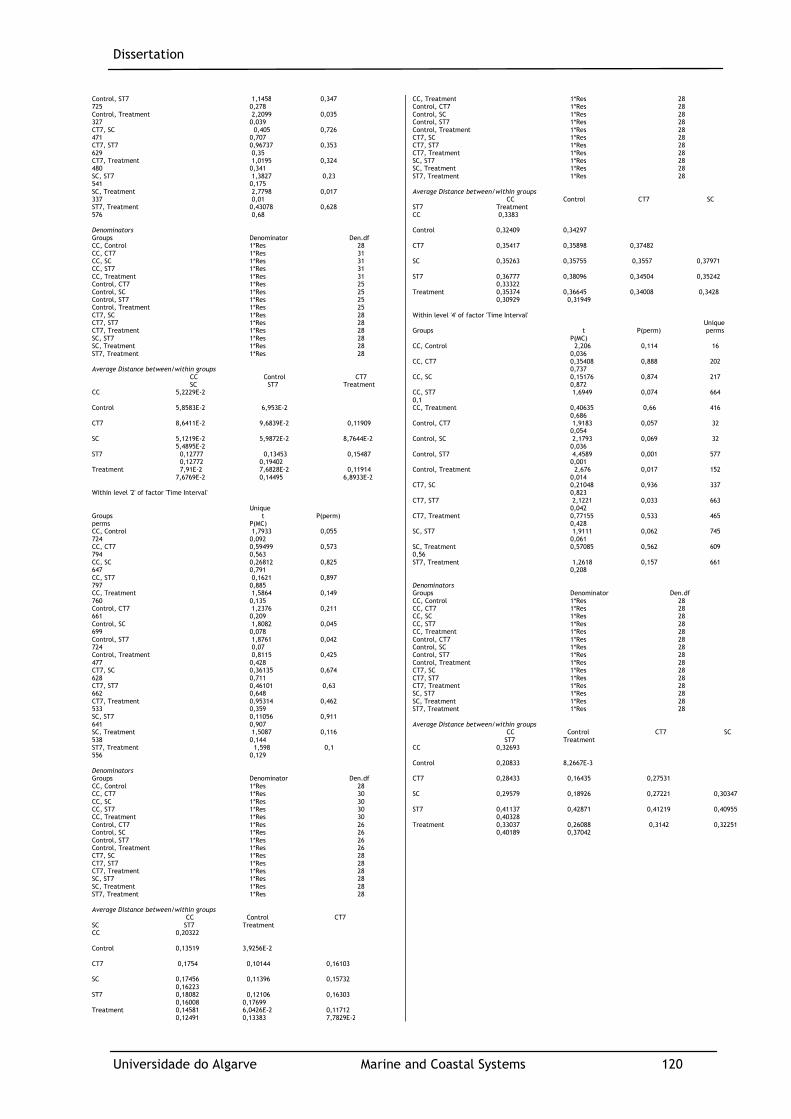
Dissertation
Universidade do Algarve Marine and Coastal Systems 120
Control, ST7 1,1458 0,347 725 0,278 Control, Treatment 2,2099 0,035 327 0,039 CT7, SC 0,405 0,726 471 0,707 CT7, ST7 0,96737 0,353 629 0,35 CT7, Treatment 1,0195 0,324 480 0,341 SC, ST7 1,3827 0,23 541 0,175 SC, Treatment 2,7798 0,017 337 0,01 ST7, Treatment 0,43078 0,628 576 0,68 Denominators Groups Denominator Den.df CC, Control 1*Res 28 CC, CT7 1*Res 31 CC, SC 1*Res 31 CC, ST7 1*Res 31 CC, Treatment 1*Res 31 Control, CT7 1*Res 25 Control, SC 1*Res 25 Control, ST7 1*Res 25 Control, Treatment 1*Res 25 CT7, SC 1*Res 28 CT7, ST7 1*Res 28 CT7, Treatment 1*Res 28 SC, ST7 1*Res 28 SC, Treatment 1*Res 28 ST7, Treatment 1*Res 28 Average Distance between/within groups CC Control CT7 SC ST7 Treatment CC 5,2229E-2 Control 5,8583E-2 6,953E-2 CT7 8,6411E-2 9,6839E-2 0,11909 SC 5,1219E-2 5,9872E-2 8,7644E-2 5,4895E-2 ST7 0,12777 0,13453 0,15487 0,12772 0,19402 Treatment 7,91E-2 7,6828E-2 0,11914 7,6769E-2 0,14495 6,8933E-2 Within level '2' of factor 'Time Interval' Unique Groups t P(perm) perms P(MC) CC, Control 1,7933 0,055 724 0,092 CC, CT7 0,59499 0,573 794 0,563 CC, SC 0,26812 0,825 647 0,791 CC, ST7 0,1621 0,897 797 0,885 CC, Treatment 1,5864 0,149 760 0,135 Control, CT7 1,2376 0,211 661 0,209 Control, SC 1,8082 0,045 699 0,078 Control, ST7 1,8761 0,042 724 0,07 Control, Treatment 0,8115 0,425 477 0,428 CT7, SC 0,36135 0,674 628 0,711 CT7, ST7 0,46101 0,63 662 0,648 CT7, Treatment 0,95314 0,462 533 0,359 SC, ST7 0,11056 0,911 641 0,907 SC, Treatment 1,5087 0,116 538 0,144 ST7, Treatment 1,598 0,1 556 0,129 Denominators Groups Denominator Den.df CC, Control 1*Res 28 CC, CT7 1*Res 30 CC, SC 1*Res 30 CC, ST7 1*Res 30 CC, Treatment 1*Res 30 Control, CT7 1*Res 26 Control, SC 1*Res 26 Control, ST7 1*Res 26 Control, Treatment 1*Res 26 CT7, SC 1*Res 28 CT7, ST7 1*Res 28 CT7, Treatment 1*Res 28 SC, ST7 1*Res 28 SC, Treatment 1*Res 28 ST7, Treatment 1*Res 28 Average Distance between/within groups CC Control CT7 SC ST7 Treatment CC 0,20322 Control 0,13519 3,9256E-2 CT7 0,1754 0,10144 0,16103 SC 0,17456 0,11396 0,15732 0,16223 ST7 0,18082 0,12106 0,16303 0,16008 0,17699 Treatment 0,14581 6,0426E-2 0,11712 0,12491 0,13383 7,7829E-2
CC, Treatment 1*Res 28 Control, CT7 1*Res 28 Control, SC 1*Res 28 Control, ST7 1*Res 28 Control, Treatment 1*Res 28 CT7, SC 1*Res 28 CT7, ST7 1*Res 28 CT7, Treatment 1*Res 28 SC, ST7 1*Res 28 SC, Treatment 1*Res 28 ST7, Treatment 1*Res 28 Average Distance between/within groups CC Control CT7 SC ST7 Treatment CC 0,3383 Control 0,32409 0,34297 CT7 0,35417 0,35898 0,37482 SC 0,35263 0,35755 0,3557 0,37971 ST7 0,36777 0,38096 0,34504 0,35242 0,33322 Treatment 0,35374 0,36645 0,34008 0,3428 0,30929 0,31949 Within level '4' of factor 'Time Interval' Unique Groups t P(perm) perms P(MC) CC, Control 2,206 0,114 16 0,036 CC, CT7 0,35408 0,888 202 0,737 CC, SC 0,15176 0,874 217 0,872 CC, ST7 1,6949 0,074 664 0,1 CC, Treatment 0,40635 0,66 416 0,686 Control, CT7 1,9183 0,057 32 0,054 Control, SC 2,1793 0,069 32 0,036 Control, ST7 4,4589 0,001 577 0,001 Control, Treatment 2,676 0,017 152 0,014 CT7, SC 0,21048 0,936 337 0,823 CT7, ST7 2,1221 0,033 663 0,042 CT7, Treatment 0,77155 0,533 465 0,428 SC, ST7 1,9111 0,062 745 0,061 SC, Treatment 0,57085 0,562 609 0,56 ST7, Treatment 1,2618 0,157 661 0,208 Denominators Groups Denominator Den.df CC, Control 1*Res 28 CC, CT7 1*Res 28 CC, SC 1*Res 28 CC, ST7 1*Res 28 CC, Treatment 1*Res 28 Control, CT7 1*Res 28 Control, SC 1*Res 28 Control, ST7 1*Res 28 Control, Treatment 1*Res 28 CT7, SC 1*Res 28 CT7, ST7 1*Res 28 CT7, Treatment 1*Res 28 SC, ST7 1*Res 28 SC, Treatment 1*Res 28 ST7, Treatment 1*Res 28 Average Distance between/within groups CC Control CT7 SC ST7 Treatment CC 0,32693 Control 0,20833 8,2667E-3 CT7 0,28433 0,16435 0,27531 SC 0,29579 0,18926 0,27221 0,30347 ST7 0,41137 0,42871 0,41219 0,40955 0,40328 Treatment 0,33037 0,26088 0,3142 0,32251 0,40189 0,37042
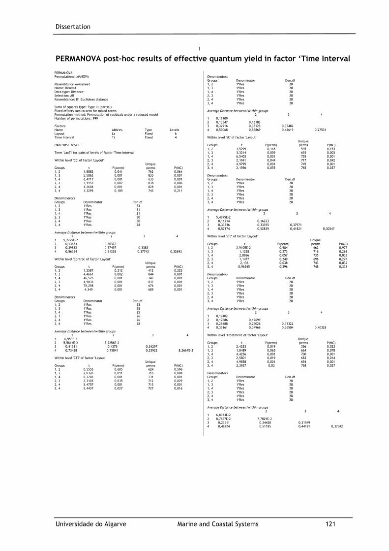
Dissertation
Universidade do Algarve Marine and Coastal Systems 121
PERMANOVA post-hoc results of effective quantum yield in factor ‘Time Interval
PERMANOVA Permutational MANOVA Resemblance worksheet Name: Resem1 Data type: Distance Selection: All Resemblance: D1 Euclidean distance Sums of squares type: Type III (partial) Fixed effects sum to zero for mixed terms Permutation method: Permutation of residuals under a reduced model Number of permutations: 999 Factors Name Abbrev. Type Levels Layout La Fixed 6 Time Interval Ti Fixed 4 PAIR-WISE TESTS Term 'LaxTi' for pairs of levels of factor 'Time Interval' Within level 'CC' of factor 'Layout' Unique Groups t P(perm) perms P(MC) 1, 2 1,8882 0,041 762 0,064 1, 3 5,5862 0,001 835 0,001 1, 4 6,4717 0,001 633 0,001 2, 3 3,1153 0,007 838 0,006 2, 4 4,2604 0,001 828 0,001 3, 4 1,3295 0,185 743 0,211 Denominators Groups Denominator Den.df 1, 2 1*Res 33 1, 3 1*Res 31 1, 4 1*Res 31 2, 3 1*Res 30 2, 4 1*Res 30 3, 4 1*Res 28 Average Distance between/within groups 1 2 3 4 1 5,2229E-2 2 0,13653 0,20322 3 0,39832 0,37497 0,3383 4 0,56354 0,51338 0,37742 0,32693 Within level 'Control' of factor 'Layout' Unique Groups t P(perm) perms P(MC) 1, 2 1,2587 0,212 412 0,225 1, 3 4,4661 0,002 844 0,001 1, 4 46,525 0,001 747 0,001 2, 3 4,9833 0,001 837 0,001 2, 4 75,298 0,001 676 0,001 3, 4 4,349 0,001 689 0,001 Denominators Groups Denominator Den.df 1, 2 1*Res 23 1, 3 1*Res 25 1, 4 1*Res 25 2, 3 1*Res 26 2, 4 1*Res 26 3, 4 1*Res 28 Average Distance between/within groups 1 2 3 4 1 6,953E-2 2 5,5814E-2 3,9256E-2 3 0,41331 0,4275 0,34297 4 0,73428 0,75841 0,33922 8,2667E-3 Within level 'CT7' of factor 'Layout' Unique Groups t P(perm) perms P(MC) 1, 2 0,5555 0,605 624 0,596 1, 3 2,8326 0,011 716 0,008 1, 4 6,2743 0,001 731 0,001 2, 3 2,3103 0,035 712 0,029 2, 4 5,4707 0,001 713 0,001 3, 4 2,4437 0,027 727 0,016
Denominators Groups Denominator Den.df 1, 2 1*Res 28 1, 3 1*Res 28 1, 4 1*Res 28 2, 3 1*Res 28 2, 4 1*Res 28 3, 4 1*Res 28 Average Distance between/within groups 1 2 3 4 1 0,11909 2 0,13547 0,16103 3 0,32916 0,33125 0,37482 4 0,59068 0,56869 0,42619 0,27531 Within level 'SC' of factor 'Layout' Unique Groups t P(perm) perms P(MC) 1, 2 1,5299 0,118 535 0,153 1, 3 3,3214 0,009 693 0,003 1, 4 6,5403 0,001 735 0,001 2, 3 2,1941 0,044 717 0,042 2, 4 4,9795 0,001 745 0,001 3, 4 2,1596 0,055 765 0,037 Denominators Groups Denominator Den.df 1, 2 1*Res 28 1, 3 1*Res 28 1, 4 1*Res 28 2, 3 1*Res 28 2, 4 1*Res 28 3, 4 1*Res 28 Average Distance between/within groups 1 2 3 4 1 5,4895E-2 2 0,11214 0,16223 3 0,33336 0,33395 0,37971 4 0,57174 0,52839 0,41821 0,30347 Within level 'ST7' of factor 'Layout' Unique Groups t P(perm) perms P(MC) 1, 2 2,9105E-2 0,984 662 0,977 1, 3 1,1228 0,273 716 0,263 1, 4 2,0866 0,057 735 0,033 2, 3 1,1477 0,249 696 0,274 2, 4 2,136 0,038 743 0,039 3, 4 0,96545 0,296 748 0,338 Denominators Groups Denominator Den.df 1, 2 1*Res 28 1, 3 1*Res 28 1, 4 1*Res 28 2, 3 1*Res 28 2, 4 1*Res 28 3, 4 1*Res 28 Average Distance between/within groups 1 2 3 4 1 0,19402 2 0,17686 0,17699 3 0,26488 0,26026 0,33322 4 0,35161 0,34966 0,36504 0,40328 Within level 'Treatment' of factor 'Layout' Unique Groups t P(perm) perms P(MC) 1, 2 2,4233 0,019 356 0,023 1, 3 1,8489 0,065 664 0,078 1, 4 4,4256 0,001 700 0,001 2, 3 2,5801 0,019 683 0,014 2, 4 4,9858 0,001 694 0,001 3, 4 2,3937 0,03 768 0,027 Denominators Groups Denominator Den.df 1, 2 1*Res 28 1, 3 1*Res 28 1, 4 1*Res 28 2, 3 1*Res 28 2, 4 1*Res 28 3, 4 1*Res 28 Average Distance between/within groups 1 2 3 4 1 6,8933E-2 2 8,7667E-2 7,7829E-2 3 0,23511 0,24428 0,31949 4 0,48224 0,51185 0,44181 0,37042
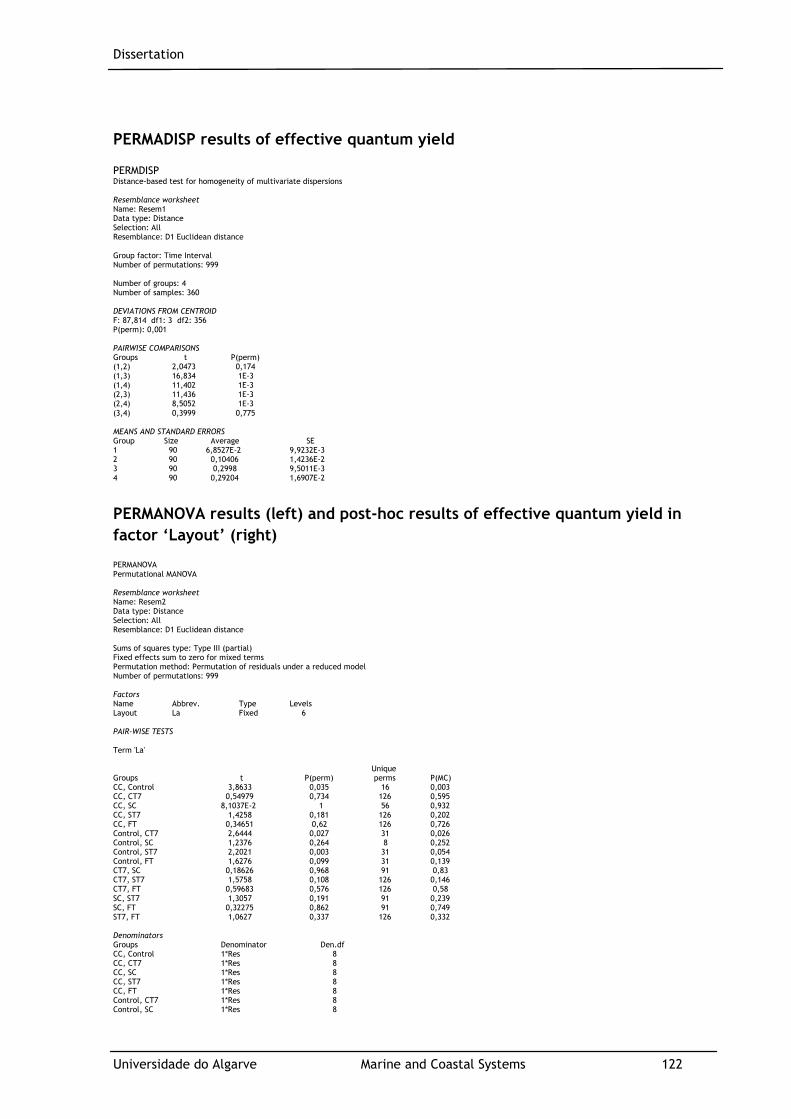
Dissertation
Universidade do Algarve Marine and Coastal Systems 122
PERMADISP results of effective quantum yield
PERMDISP Distance-based test for homogeneity of multivariate dispersions Resemblance worksheet Name: Resem1 Data type: Distance Selection: All Resemblance: D1 Euclidean distance Group factor: Time Interval Number of permutations: 999 Number of groups: 4 Number of samples: 360 DEVIATIONS FROM CENTROID F: 87,814 df1: 3 df2: 356 P(perm): 0,001 PAIRWISE COMPARISONS Groups t P(perm) (1,2) 2,0473 0,174 (1,3) 16,834 1E-3 (1,4) 11,402 1E-3 (2,3) 11,436 1E-3 (2,4) 8,5052 1E-3 (3,4) 0,3999 0,775 MEANS AND STANDARD ERRORS Group Size Average SE 1 90 6,8527E-2 9,9232E-3 2 90 0,10406 1,4236E-2 3 90 0,2998 9,5011E-3 4 90 0,29204 1,6907E-2
PERMANOVA results (left) and post-hoc results of effective quantum yield in
factor ‘Layout’ (right)
PERMANOVA Permutational MANOVA Resemblance worksheet Name: Resem2 Data type: Distance Selection: All Resemblance: D1 Euclidean distance Sums of squares type: Type III (partial) Fixed effects sum to zero for mixed terms Permutation method: Permutation of residuals under a reduced model Number of permutations: 999 Factors Name Abbrev. Type Levels Layout La Fixed 6 PAIR-WISE TESTS Term 'La' Unique Groups t P(perm) perms P(MC) CC, Control 3,8633 0,035 16 0,003 CC, CT7 0,54979 0,734 126 0,595 CC, SC 8,1037E-2 1 56 0,932 CC, ST7 1,4258 0,181 126 0,202 CC, FT 0,34651 0,62 126 0,726 Control, CT7 2,6444 0,027 31 0,026 Control, SC 1,2376 0,264 8 0,252 Control, ST7 2,2021 0,003 31 0,054 Control, FT 1,6276 0,099 31 0,139 CT7, SC 0,18626 0,968 91 0,83 CT7, ST7 1,5758 0,108 126 0,146 CT7, FT 0,59683 0,576 126 0,58 SC, ST7 1,3057 0,191 91 0,239 SC, FT 0,32275 0,862 91 0,749 ST7, FT 1,0627 0,337 126 0,332 Denominators Groups Denominator Den.df CC, Control 1*Res 8 CC, CT7 1*Res 8 CC, SC 1*Res 8 CC, ST7 1*Res 8 CC, FT 1*Res 8 Control, CT7 1*Res 8 Control, SC 1*Res 8

Dissertation
Universidade do Algarve Marine and Coastal Systems 123
Control, ST7 1*Res 8 Control, FT 1*Res 8 CT7, SC 1*Res 8 CT7, ST7 1*Res 8 CT7, FT 1*Res 8 SC, ST7 1*Res 8 SC, FT 1*Res 8 ST7, FT 1*Res 8 Average Distance between/within groups CC Control CT7 SC ST7 FT CC 15,951 Control 27,625 1,146 CT7 16,192 21,564 21,047 SC 35,338 26,232 33,166 47,421 ST7 61,776 80,43 65,583 74,864 95,539 FT 40,205 35,67 38,708 43,364 73,118 54,97
PERMADISP results of effective quantum yield
PERMDISP Distance-based test for homogeneity of multivariate dispersions Resemblance worksheet Name: Resem2 Data type: Distance Selection: All Resemblance: D1 Euclidean distance Group factor: Layout Number of permutations: 999 Number of groups: 6 Number of samples: 30 DEVIATIONS FROM CENTROID F: 4,9933 df1: 5 df2: 24 P(perm): 0,046 PAIRWISE COMPARISONS Groups t P(perm) (CC,Control) 2,3697 6E-3 (CC,CT7) 0,96767 0,718 (CC,SC) 1,5566 0,17 (CC,ST7) 2,556 1,5E-2 (CC,FT) 3,953 9E-3 (Control,CT7) 7,6773 1,1E-2 (Control,SC) 2,4369 1,4E-2 (Control,ST7) 3,1485 7E-3 (Control,FT) 6,4012 1E-2 (CT7,SC) 1,2738 0,385 (CT7,ST7) 2,3715 1,2E-2 (CT7,FT) 3,8928 9E-3 (SC,ST7) 1,2697 0,442 (SC,FT) 0,63369 0,598 (ST7,FT) 1,0033 0,549 MEANS AND STANDARD ERRORS Group Size Average SE CC 5 11,187 4,3205 Control 5 0,91682 0,34381 CT7 5 15,755 1,902 SC 5 32,365 12,901 ST7 5 61,916 19,371 FT 5 41,47 6,326
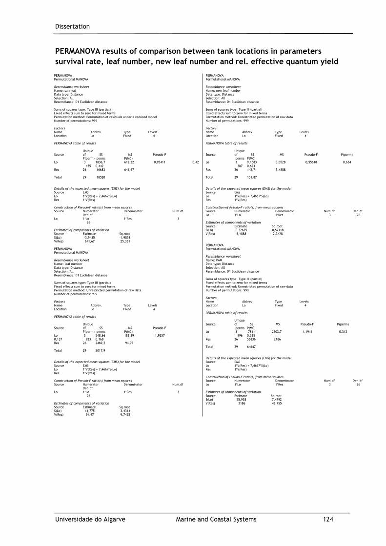
Dissertation
Universidade do Algarve Marine and Coastal Systems 124
PERMANOVA results of comparison between tank locations in parameters
survival rate, leaf number, new leaf number and rel. effective quantum yield
PERMANOVA Permutational MANOVA Resemblance worksheet Name: survival Data type: Distance Selection: All Resemblance: D1 Euclidean distance Sums of squares type: Type III (partial) Fixed effects sum to zero for mixed terms Permutation method: Permutation of residuals under a reduced model Number of permutations: 999 Factors Name Abbrev. Type Levels Location Lo Fixed 4 PERMANOVA table of results Unique Source df SS MS Pseudo-F P(perm) perms P(MC) Lo 3 1836,7 612,22 0,95411 0,42 155 0,442 Res 26 16683 641,67 Total 29 18520 Details of the expected mean squares (EMS) for the model Source EMS Lo 1*V(Res) + 7,4667*S(Lo) Res 1*V(Res) Construction of Pseudo-F ratio(s) from mean squares Source Numerator Denominator Num.df Den.df Lo 1*Lo 1*Res 3 26 Estimates of components of variation Source Estimate Sq.root S(Lo) -3,9435 -1,9858 V(Res) 641,67 25,331 PERMANOVA Permutational MANOVA Resemblance worksheet Name: leaf number Data type: Distance Selection: All Resemblance: D1 Euclidean distance Sums of squares type: Type III (partial) Fixed effects sum to zero for mixed terms Permutation method: Unrestricted permutation of raw data Number of permutations: 999 Factors Name Abbrev. Type Levels Location Lo Fixed 4 PERMANOVA table of results Unique Source df SS MS Pseudo-F P(perm) perms P(MC) Lo 3 548,66 182,89 1,9257 0,137 923 0,168 Res 26 2469,2 94,97 Total 29 3017,9 Details of the expected mean squares (EMS) for the model Source EMS Lo 1*V(Res) + 7,4667*S(Lo) Res 1*V(Res) Construction of Pseudo-F ratio(s) from mean squares Source Numerator Denominator Num.df Den.df Lo 1*Lo 1*Res 3 26 Estimates of components of variation Source Estimate Sq.root S(Lo) 11,775 3,4314 V(Res) 94,97 9,7452
PERMANOVA Permutational MANOVA Resemblance worksheet Name: new leaf number Data type: Distance Selection: All Resemblance: D1 Euclidean distance Sums of squares type: Type III (partial) Fixed effects sum to zero for mixed terms Permutation method: Unrestricted permutation of raw data Number of permutations: 999 Factors Name Abbrev. Type Levels Location Lo Fixed 4 PERMANOVA table of results Unique Source df SS MS Pseudo-F P(perm) perms P(MC) Lo 3 9,1583 3,0528 0,55618 0,634 387 0,623 Res 26 142,71 5,4888 Total 29 151,87 Details of the expected mean squares (EMS) for the model Source EMS Lo 1*V(Res) + 7,4667*S(Lo) Res 1*V(Res) Construction of Pseudo-F ratio(s) from mean squares Source Numerator Denominator Num.df Den.df Lo 1*Lo 1*Res 3 26 Estimates of components of variation Source Estimate Sq.root S(Lo) -0,32625 -0,57118 V(Res) 5,4888 2,3428 PERMANOVA Permutational MANOVA Resemblance worksheet Name: PAM Data type: Distance Selection: All Resemblance: D1 Euclidean distance Sums of squares type: Type III (partial) Fixed effects sum to zero for mixed terms Permutation method: Unrestricted permutation of raw data Number of permutations: 999 Factors Name Abbrev. Type Levels Location Lo Fixed 4 PERMANOVA table of results Unique Source df SS MS Pseudo-F P(perm) perms P(MC) Lo 3 7811 2603,7 1,1911 0,312 996 0,335 Res 26 56836 2186 Total 29 64647 Details of the expected mean squares (EMS) for the model Source EMS Lo 1*V(Res) + 7,4667*S(Lo) Res 1*V(Res) Construction of Pseudo-F ratio(s) from mean squares Source Numerator Denominator Num.df Den.df Lo 1*Lo 1*Res 3 26 Estimates of components of variation Source Estimate Sq.root S(Lo) 55,938 7,4792 V(Res) 2186 46,755
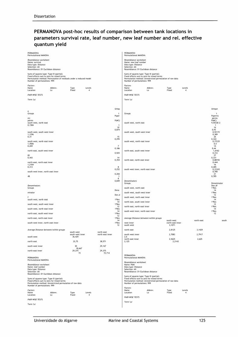
Dissertation
Universidade do Algarve Marine and Coastal Systems 125
PERMANOVA post-hoc results of comparison between tank locations in
parameters survival rate, leaf number, new leaf number and rel. effective
quantum yield
PERMANOVA Permutational MANOVA Resemblance worksheet Name: survival Data type: Distance Selection: All Resemblance: D1 Euclidean distance Sums of squares type: Type III (partial) Fixed effects sum to zero for mixed terms Permutation method: Permutation of residuals under a reduced model Number of permutations: 999 Factors Name Abbrev. Type Levels Location Lo Fixed 4 PAIR-WISE TESTS Term 'Lo' Unique Groups t P(perm) perms P(MC) south west, north east 0,1584 1 10 0,874 south west, south west inner 1,1296 0,31 15 0,295 south west, north east inner 1,4506 0,269 7 0,186 north east, south west inner 0,92582 0,443 14 0,354 north east, north east inner 1,2104 0,313 8 0,252 south west inner, north east inner 0,20448 1 8 0,849 Denominators Groups Denominator Den.df south west, north east 1*Res 14 south west, south west inner 1*Res 12 south west, north east inner 1*Res 14 north east, south west inner 1*Res 12 north east, north east inner 1*Res 14 south west inner, north east inner 1*Res 12 Average Distance between/within groups south west north east south west inner north east inner south west 36,429 north east 33,75 38,571 south west inner 30 29,167 18,667 north east inner 29,375 29,375 15 15,714 PERMANOVA Permutational MANOVA Resemblance worksheet Name: leaf number Data type: Distance Selection: All Resemblance: D1 Euclidean distance Sums of squares type: Type III (partial) Fixed effects sum to zero for mixed terms Permutation method: Unrestricted permutation of raw data Number of permutations: 999 Factors Name Abbrev. Type Levels Location Lo Fixed 4 PAIR-WISE TESTS Term 'Lo'
PERMANOVA Permutational MANOVA Resemblance worksheet Name: new leaf number Data type: Distance Selection: All Resemblance: D1 Euclidean distance Sums of squares type: Type III (partial) Fixed effects sum to zero for mixed terms Permutation method: Unrestricted permutation of raw data Number of permutations: 999 Factors Name Abbrev. Type Levels Location Lo Fixed 4 PAIR-WISE TESTS Term 'Lo' Unique Groups t P(perm) perms P(MC) south west, north east 9,5533E-2 1 16 0,93 south west, south west inner 0,92172 0,389 26 0,344 south west, north east inner 0,77235 0,5 14 0,44 north east, south west inner 1,0162 0,312 27 0,331 north east, north east inner 0,88192 0,444 16 0,405 south west inner, north east inner 0,31243 0,785 21 0,785 Denominators Groups Denominator Den.df south west, north east 1*Res 14 south west, south west inner 1*Res 12 south west, north east inner 1*Res 14 north east, south west inner 1*Res 12 north east, north east inner 1*Res 14 south west inner, north east inner 1*Res 12 Average Distance between/within groups south west north east south west inner north east inner south west 3,1071 north east 2,8125 3,1429 south west inner 2,7083 2,7917 2,6 north east inner 2,5625 2,625 2,125 2,2143 PERMANOVA Permutational MANOVA Resemblance worksheet Name: PAM Data type: Distance Selection: All Resemblance: D1 Euclidean distance Sums of squares type: Type III (partial) Fixed effects sum to zero for mixed terms Permutation method: Unrestricted permutation of raw data Number of permutations: 999 Factors Name Abbrev. Type Levels Location Lo Fixed 4 PAIR-WISE TESTS Term 'Lo'
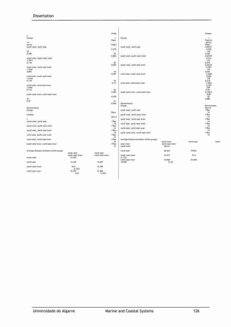
Dissertation
Universidade do Algarve Marine and Coastal Systems 126
Unique Groups t P(perm) perms P(MC) south west, north east 0,27052 0,789 53 0,803 south west, south west inner 1,7813 0,116 42 0,093 south west, north east inner 1,7647 0,095 44 0,097 north east, south west inner 1,6124 0,119 53 0,14 north east, north east inner 1,6581 0,112 56 0,095 south west inner, north east inner 0,59593 0,57 31 0,564 Denominators Groups Denominator Den.df south west, north east 1*Res 14 south west, south west inner 1*Res 12 south west, north east inner 1*Res 14 north east, south west inner 1*Res 12 north east, north east inner 1*Res 14 south west inner, north east inner 1*Res 12 Average Distance between/within groups south west north east south west inner north east inner south west 12,429 north east 13,438 16,857 south west inner 10,5 12,708 3,1333 north east inner 10,375 12,406 3,25 4,1071
Unique Groups t P(perm) perms P(MC) south west, north east 0,85511 0,458 139 0,383 south west, south west inner 0,67219 0,512 124 0,519 south west, north east inner 0,69232 0,505 147 0,493 north east, south west inner 1,2928 0,266 138 0,218 north east, north east inner 1,4455 0,182 209 0,19 south west inner, north east inner 0,14673 0,89 82 0,889 Denominators Groups Denominator Den.df south west, north east 1*Res 14 south west, south west inner 1*Res 12 south west, north east inner 1*Res 14 north east, south west inner 1*Res 12 north east, north east inner 1*Res 14 south west inner, north east inner 1*Res 12 Average Distance between/within groups south west north east south west inner north east inner south west 48,321 north east 60,563 79,821 south west inner 34,917 53,5 21,733 north east inner 34,969 53,594 18,958 21,25
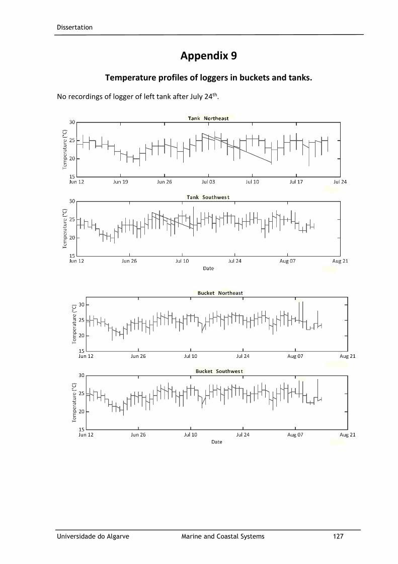
Dissertation
Universidade do Algarve Marine and Coastal Systems 127
Appendix 9
Temperature profiles of loggers in buckets and tanks.
No recordings of logger of left tank after July 24th.

Dissertation
Universidade do Algarve Marine and Coastal Systems 128
Appendix 10
Zostera marina shoots before (left) and after (right) the experiment
CC
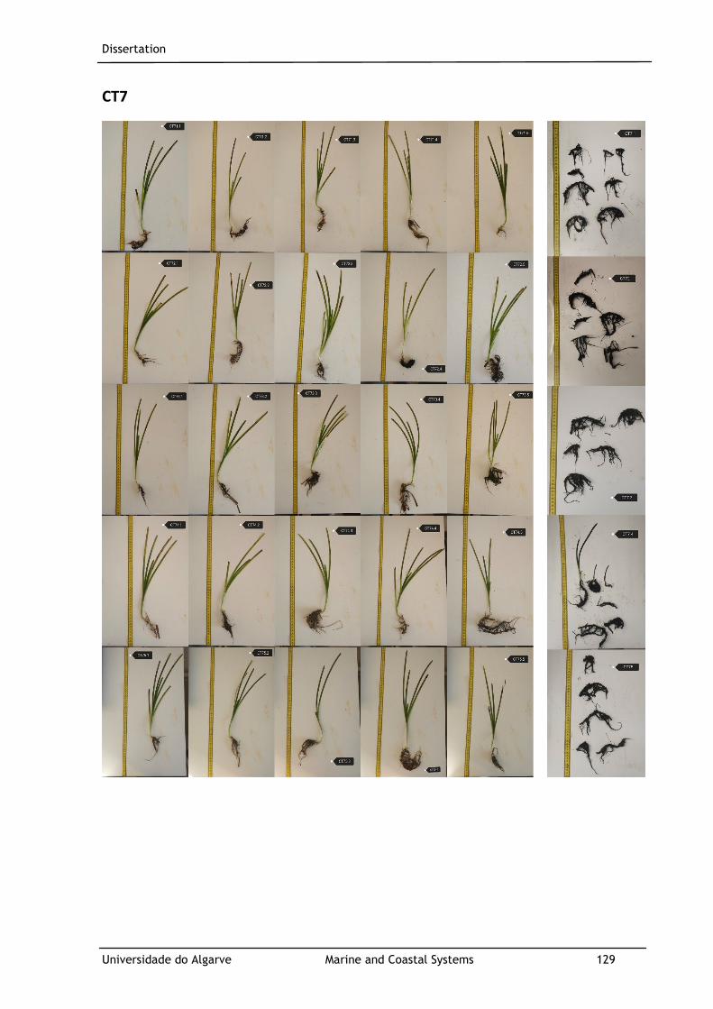
Dissertation
Universidade do Algarve Marine and Coastal Systems 129
CT7
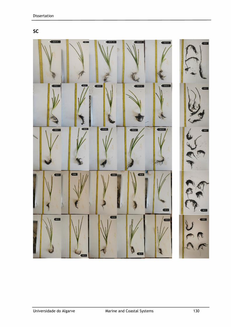
Dissertation
Universidade do Algarve Marine and Coastal Systems 130
SC
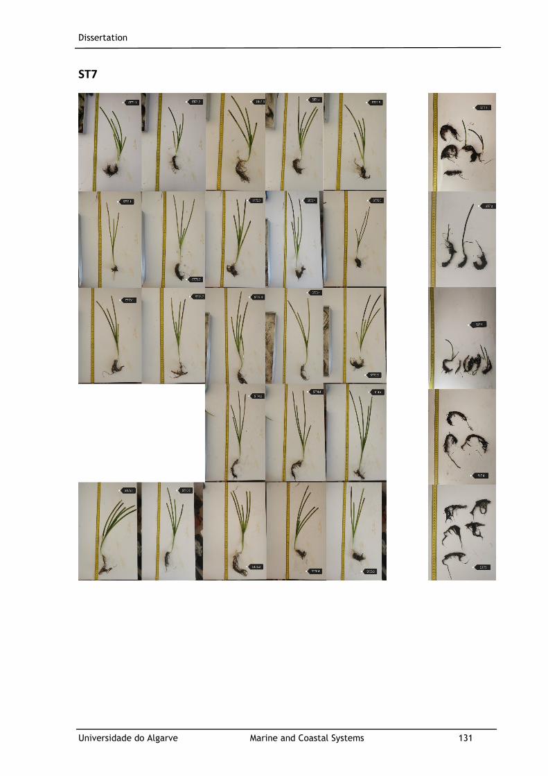
Dissertation
Universidade do Algarve Marine and Coastal Systems 131
ST7

Dissertation
Universidade do Algarve Marine and Coastal Systems 132
Control
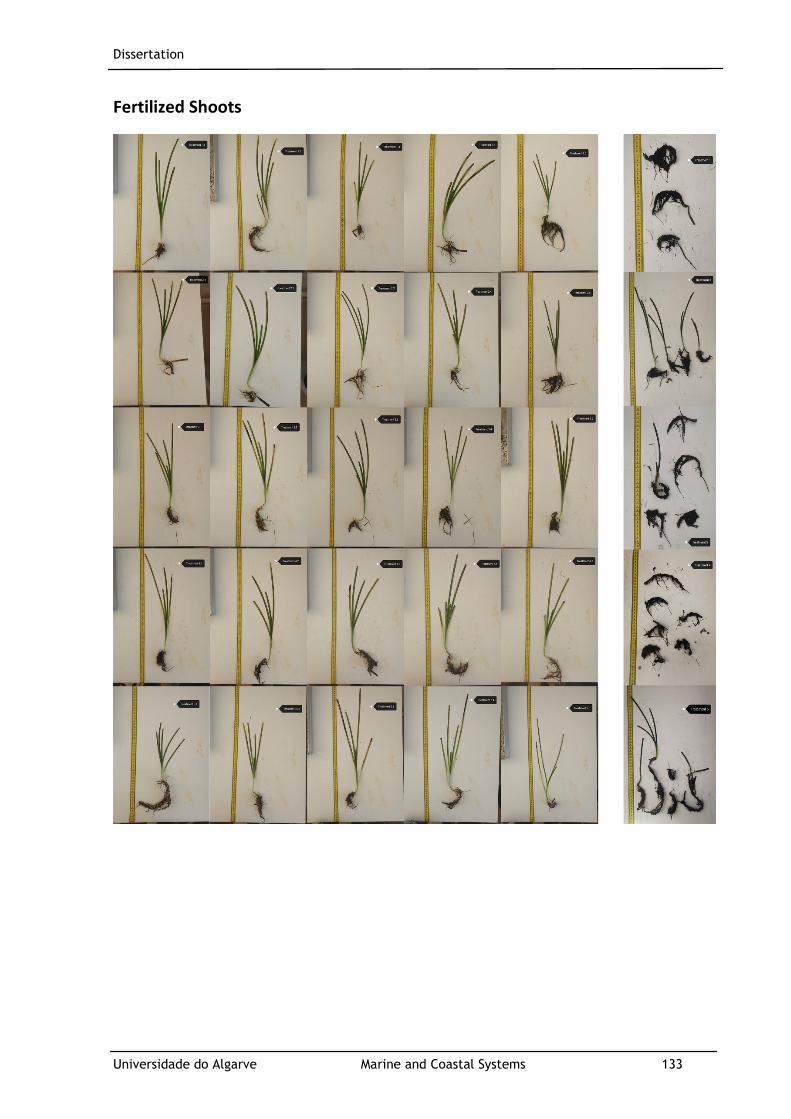
Dissertation
Universidade do Algarve Marine and Coastal Systems 133
Fertilized Shoots
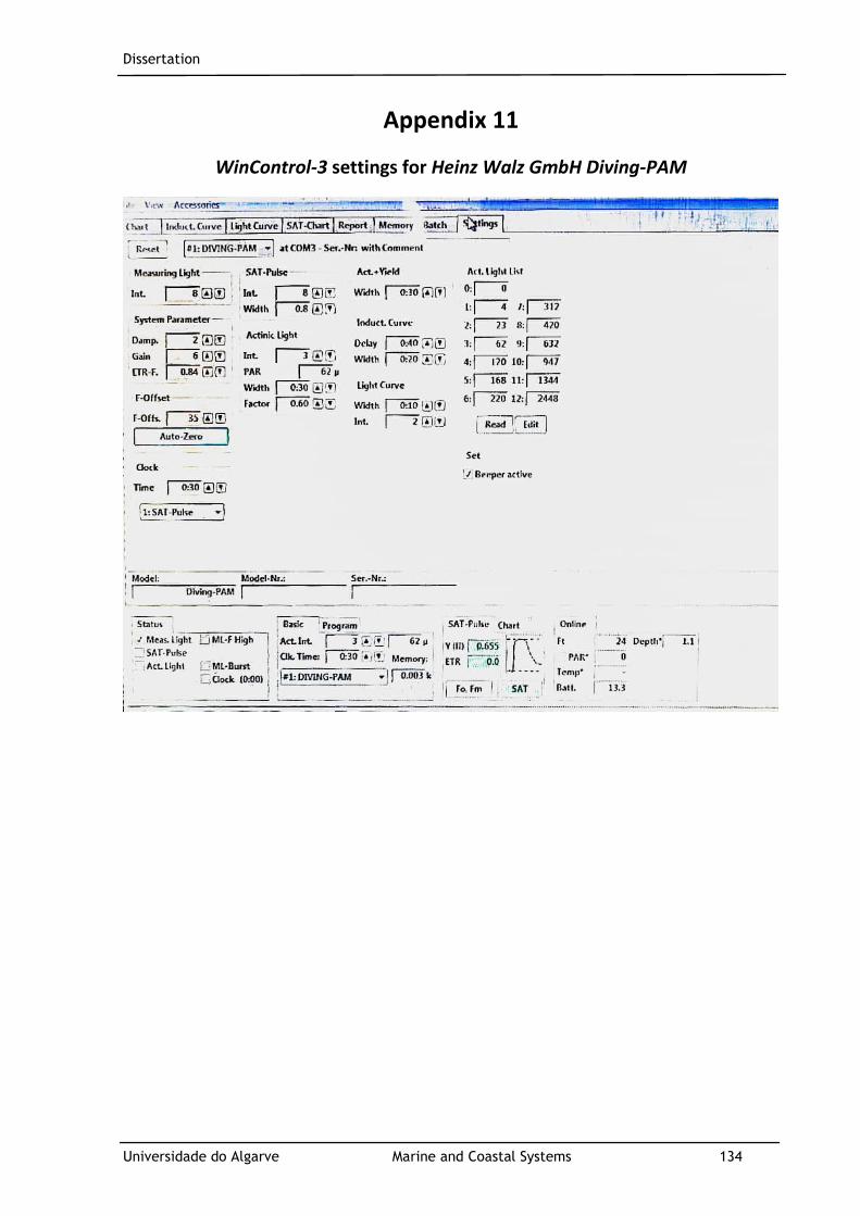
Dissertation
Universidade do Algarve Marine and Coastal Systems 134
Appendix 11
WinControl-3 settings for Heinz Walz GmbH Diving-PAM
Related Documents


