Sand production simulation coupling DEM with CFD

European Journal of Environmental andCivil EngineeringPublication details, including instructions for authors andsubscription information:http://www.tandfonline.com/loi/tece20

Sand production simulation couplingDEM with CFDNatalia Climenta, Marcos Arroyoa, Catherine O’Sullivanb & AntonioGensa

a Department of Geotechnical Engineering, Technical University ofCatalonia, Barcelona, Spainb Department of Civil and Environmental Engineering, ImperialCollege London, London, UKPublished online: 29 May 2014.

To cite this article: Natalia Climent, Marcos Arroyo, Catherine O’Sullivan & Antonio Gens (2014):Sand production simulation coupling DEM with CFD, European Journal of Environmental and CivilEngineering, DOI: 10.1080/19648189.2014.920280

To link to this article: http://dx.doi.org/10.1080/19648189.2014.920280

PLEASE SCROLL DOWN FOR ARTICLE

Taylor & Francis makes every effort to ensure the accuracy of all the information (the“Content”) contained in the publications on our platform. However, Taylor & Francis,our agents, and our licensors make no representations or warranties whatsoever as tothe accuracy, completeness, or suitability for any purpose of the Content. Any opinionsand views expressed in this publication are the opinions and views of the authors,and are not the views of or endorsed by Taylor & Francis. The accuracy of the Contentshould not be relied upon and should be independently verified with primary sourcesof information. Taylor and Francis shall not be liable for any losses, actions, claims,proceedings, demands, costs, expenses, damages, and other liabilities whatsoever orhowsoever caused arising directly or indirectly in connection with, in relation to or arisingout of the use of the Content.

This article may be used for research, teaching, and private study purposes. Anysubstantial or systematic reproduction, redistribution, reselling, loan, sub-licensing,systematic supply, or distribution in any form to anyone is expressly forbidden. Terms &

Conditions of access and use can be found at http://www.tandfonline.com/page/terms-and-conditions

Sand production simulation coupling DEM with CFD

Natalia Climenta*, Marcos Arroyoa, Catherine O’Sullivanb and Antonio Gensa

aDepartment of Geotechnical Engineering, Technical University of Catalonia, Barcelona, Spain;bDepartment of Civil and Environmental Engineering, Imperial College London, London, UK

(Received 4 June 2013; accepted 26 April 2014)

Sand production in oil wells is often predicted using continuum fluid-coupled models.However, a continuum approach cannot capture important features of the sandingproblem, such as erosion and localised failure. This shortcoming of continuum-basedanalyses can be overcome using the particulate discrete element method (DEM). How-ever, these models, apart from issues of computational cost, have the disadvantage ofbeing difficult to calibrate. One way forward is to calibrate DEM models to capturethe response observed in continuum models, where the material parameters can beselected with greater confidence. Adopting this philosophy here, a 3D numericalmodel based on DEM coupled with Computational Fluid Dynamics was built to simu-late sand production around perforations. In the first instance, the basic DEM model(i.e. a dry case) is calibrated against a well-known poro-elastoplastic analytical solu-tion by Risnes et al. (1982). Subsequently, a range of hydrostatic scenarios involvingdifferent levels of pore pressure and effective stress are considered. The numericalmodel shows an asymmetry of the eroded zone that is related to initial microscaleinhomogeneity. The stress peak of the analytical solution at the elastic-plastic interfaceis smoothed because of that asymmetry. The presence of hydrostatic fluid decreasesthe plastic region and reduces the amount of sand produced. This is not due tochanges in effective stress but rather by the particle-scale stabilizing effect of the fluiddrag.

Keywords: discrete element method; Computational Fluid Dynamics; CFD-DEM;coupling; sand production

1. Introduction

The sand production mechanism considered here is the erosion of formation particlesdue to fluid flow during hydrocarbon recovery from sandstone reservoirs. The problemis most pronounced in weakly consolidated sandstones which, when affected, are thensaid to produce sand. In order to recover the hydrocarbon, a well needs to be drilled tothe depth of the reservoir. The well is then either left uncased (in natural completions)or cemented, cased and later perforated. In either case, the sandstone is left unsupported(by solid material) next to a cavity; these are the locations where sand grains can bedislodged and entered into the oil recovery system. The rock around the wellbore isweakened due to the stress concentrations around the cavity. The weakened and decohe-sioned sandstone may be eroded away by the produced fluid.

Several problems may arise due to sand production; these include clogging up ofthe well, damage to the well equipment, well instability due to the loss of material

*Corresponding author. Email: [email protected]

© 2014 Taylor & Francis

European Journal of Environmental and Civil Engineering, 2014http://dx.doi.org/10.1080/19648189.2014.920280

Do

damage to the formation, etc. Consequently, studying the sand production process anddeveloping methods to control sanding are of paramount importance for safe andeconomical hydrocarbon production.

1.1. Mechanisms of sand production

Sand production is a coupled fluid–solid process that primarily involves two mecha-nisms (Fjær, Holt, Horsrud, Raaen, & Risnes, 2008): mechanical instabilities that leadto localised plastic behaviour and failure of the rock around the cavity, and the subse-quent transportation of sand particles due to the fluid drag forces. The sandstone rockinitially fails close to the cavity and the failed material is then eroded by the flowingfluid. These two mechanisms are coupled, since stress concentrations around the erodedcavity lead to increased damage, which in turn, increases the amount of cohesionlessmaterial that can be dislodged. The classical approach focuses on the conditions trigger-ing sand production, identifying several failure modes (e.g. tension, shear, compression)the conditions in which they are relevant and the controlling operative variables (e.g.drawdown).

More recent approaches try to follow the process further, and also predict the rate atwhich sand is produced. Internal erosion is then also a relevant mechanism as proposedby Papamichos, Vardoulakis, Tronvoll, and Skjirstein (2001) and Papamichos andVardoulakis (2005). Erosion occurs when the drag force by the fluid is sufficient toovercome the cohesive and frictional strength of the material and carry the particlesaway. Moreover, finer particles from deeper within the formation can also be transportedby the fluid. These finer particles can be made up of the original depositional materialor maybe created by particle breakage due to the increase in the effective stress withinthe formation during the oil recovery process. Redeposition of the eroded material inthe vicinity of the cavity is also possible, with implications for stability and flowrate.

1.2. Numerical methods for predicting sand production

While both experimental and analytical models of the sand production problem play animportant role, the development of numerical models is essential for realistic predictions(Rahmati et al., 2013). The vast majority of the numerical models that have been usedto date are continuum based. Using a continuum model, several constitutive relationsare necessary: a stress–strain relation for the solid skeleton, a description of fluid flowthrough the porous material, a coupling between flow and skeleton stress variables (e.g.an effective stress definition) and a sanding criterion to identify the volume of sand pro-duced. While some good results have been obtained (e.g. Nouri, Vaziri, Kuru, & Islam,2006; Papamichos & Vardoulakis, 2005), it is recognised that the formulation and verifi-cation of those constitutive relations remain a difficult task, because of the large numberof interactions and non-linearities intrinsic to the problem (e.g. non-Darcian flow; brittlefracture, etc.). Other fundamental issues of continuum numerical approaches are also rel-evant in this problem: treatment of localizations, use of Lagrangian or Eulerian formula-tions, treatment of produced zones, etc.

These difficulties have motivated the use of particle-scale simulations, which byredefining the fluid and/or the solid physics at the micro-scale allow a simpler formula-tion of the problem and a better understanding of some of its features. For instance, thedisaggregation of particles from the rock mass and its transport through the pore struc-ture can be described in discrete element method (DEM) models. However, even where

2 N. Climent et al.

4

DEM is used a number of constitutive choices remain, these include the solid–solidcontact law; fluid–solid interaction. Analysts can also choose to use either a 2D or 3Dmodel. Therefore, models of the problem have been proposed with different focus andfeatures. Indeed, the large majority of these studies (e.g. Boutt, Cook, & Williams,2011; Cook, Noble, & Williams, 2004; Dorfmann, Rothenburg, & Bruno, 1997; Marrion& Woods, 2009; O’Connor, Torczynski, Preece, Klosek, & Williams, 1997; Quadros,Vargas, Gonçalves, & Prestes, 2010) have been performed on 2D discrete models; thesecertainly offer qualitative insight, but they produce results which are difficult to relatequantitatively to field or experimental observations. Other studies have used 3D parti-cles, but have focused on small-scale phenomena involving only a few particles (Grof,Cook, Lawrence, & Štěpánek, 2009) or have radically simplified some aspect of theproblem, such as the flow pattern (1D flow, Cheung, 2010) or the boundary conditions(Zhou, Yu, & Choi, 2011). One particular area in which little systematic work has beendone is in the comparison or cross-validation of continuum and discrete models, whichis the focus of this paper.

2. The numerical method: CFD-DEM

2.1. Discrete element method

DEM was proposed originally by Cundall and Strack (1979) and is widely used tomodel soils and rocks, including sandstone (e.g. Cheung, O’Sullivan, & Coop, 2013;Potyondy & Cundall, 2004). In this study, the 3D DEM code, PFC3D (Particle-FlowCode 3D), is used (Itasca, 2008a). The basic discrete elements are spherical particles.Model boundaries are defined by introducing wall elements, to which displacement ratescan be imposed. Boundary stress values are applied using a servo-controlled algorithmto adjust wall displacement.

Particle motion is described by Newton’s second law. The relevant governing equa-tions for translational and rotational motion of a particle i with mass mi, and rotationalinertia Ii, are

midvidt

¼Xj

Fcij þ Fg

i þ Fei þ Fd

i (1)

Iidxi

dt¼Xj

Mij (2)

where vi and xi are the translational and angular velocities of particle i, respectively, Fcij

and Mij are the force and torque acting on particle i due to contact j with other particlesor walls, Fg

i is the gravitational force, Fei is the total external force acting on particle i

by other sources (e.g. fluid interaction, see below) and Fdi is a local damping force.

In DEM, some dissipation mechanisms, like contact friction, are explicitly modelled.Local damping accounts for dissipation mechanisms that are not explicitly modelled.The local damping formulation used in PFC3D is similar to that described in Cundall(1987):

Fd ¼ �djFjsignðvÞ (3)

where δ is the damping constant, v is the particle velocity, F represents the sum of allother forces acting on a particle (contact forces, gravitational force and external forces)and sign(v) is +1 when v > 0, −1 when v < 0, and 0 when v = 0.

European Journal of Environmental and Civil Engineering 3

In this study, the linear and parallel-bond contact models are used. In the linearcontact model, the load displacement relationship between two contacting bodies isrepresented by linear springs. The three input parameters are the particle normal andshear stiffness, KN and KS, and the inter-particle friction coefficient μ. The stiffness isconstant for each particle.

The parallel-bond contact model is described in detail by Potyondy and Cundall(2004). This contact model aims to represent the main mechanical effects of a finiteamount of cementing material deposited between particles. Effects considered importantinclude the contact’s tensile strength, the (cohesive) shear strength and rotational resis-tance. It is important to note that in addition to normal and tangential forces, momentscan also be transferred between the bonded particles. Cementation between particles isalso assumed to change the contact stiffness; hence, the model includes a set of normaland tangential springs, acting in parallel with those describing the linear contact model.

When the forces acting on the parallel bond reach either of its strength limits, theparallel bond is erased and cannot be reformed, even if contact between these two parti-cles is re-established at a later point. Using this approximation, forces due to the cemen-tation between particles can be modelled without representing explicitly the mass orvolume of the bonding agent.

The parameters required to define a parallel-bond are: the parallel-bond normal stiff-ness (KN

pb, in Pa m−1), the parallel-bond shear (tangential) stiffness (KSpb, in Pa m−1), the

parallel-bond normal strength (SNpb, Pa), the parallel-bond shear strength (SSpb, in Pa) andthe degree of bonding (abond). Overviews of the relation between the various inputparameters and the overall material response are given in Potyondy and Cundall (2004)and Cheung et al. (2013).

A DEM model is explicit and uses the Verlet time integration approach. The DEMtime step used in this model is the default time step calculated by PFC3D (Itasca,2008a). A critical time step is calculated for each particle following

tcrit ¼ffiffiffiffiffiffiffiffiffim=k

p(4)

where m is the mass of the particle and k is the stiffness of the contact. Then, the mini-mum critical time step of the entire system is used as simulation time step. After eachDEM cycle, this time step is recalculated.

2.2. Computational Fluid Dynamics

Computational Fluid Dynamics (CFD) is the technique of obtaining numerical approxi-mate solutions to problems involving fluid motion (Ferziger & Perić, 1999). Suchmotions are ruled by well-established differential equations of fluid mechanics, whichare approximated using different discretization techniques. Here, we assume the fluid isNewtonian and incompressible and the motion is described by the Navier Stokes equa-tion (conservation of momentum, Equation (5)) and the continuity equation (conserva-tion of mass, Equation (6)).

qf@u

@tþ qf urðuÞ ¼ �rpþ lr2ðuÞ þ qf g (5)

r � u ¼ 0 (6)

4 N. Climent et al.

4

where ρf is the fluid density, u is the fluid velocity, p is the fluid pressure and μ is thefluid viscosity. Additional boundary and initial conditions are necessary to fully specifythe mathematical problem for a given domain.

CFD is performed in this study using the code coupled computational fluid dynam-ics (CCFD), developed by ITOCHU Techno-Solution Corporation (Itasca, 2008b). InCCFD, discretization of the governing equations is achieved using a finite volume tech-nique. At every hexahedral cell in the grid, a single value represents each of the fluidproperties and state variables (velocity, pressure). CCFD calculates fluid velocity andpressure at the centre of each cell. When required, pressure values the centre of the cellfaces are interpolated from those calculated at cell centres.

Time integration in CCFD can be implicit or explicit. For this work, explicit timeintegration was used. The CFD time step required is the minimum half-cell time for allthe cells in the grid. The half-cell time, Δtcfd, is computed at each cell as

Dtcfd ¼ 1

2

Dxcfdu

(7)

where Δxcfd is the size of the cell and u is the fluid velocity in each cell (Itasca, 2008b).After each CFD calculation cycle, the CFD time step is recalculated.

More algorithmic details of the CFD method used by CCFD are given in Itasca(2008b). CCFD was initially designed and applied for problems of fluid-structure inter-action and was later integrated as add-on to PFC3D to enable coupled fluid-particle mod-elling.

2.3. Fluid-particle coupling using CFD-DEM

In general, particles in granular materials are surrounded by fluid. In some problems,the interaction between particles and fluid controls the mechanical behaviour. To simu-late this interaction at the soil particle scale, the solid DEM model must be coupled witha fluid model and several fluid-coupling techniques are available (Zhu, Zhou, Yang, &Yu, 2007). An important difference between the available coupling approaches is thedifferent length and time scales at which they aim to solve the fluid mechanics. Someapproaches (e.g. Grof et al., 2009) model the fluid flow details at the sub-particle scale,and therefore they use a description of fluid-particle interaction at the single particlelevel. This is computationally intensive and quickly reduces the extent of a feasiblemodel. One possible alternative, still at the pore-scale, is presented by (Catalano,Chareyre, & Barthélémy, 2013) who use a finite volume method (PFV) to represent thevoid space as a network of connected pores and throats.

“Mesoscopic” coupling schemes, on the other hand, establish the coupling at a largerscale, thus reducing the computational expense and allowing the creation of larger models.The method used here uses mesoscopic coupling and is known as CFD-DEM (Zhu et al.,2007). CFD-DEM was pioneered by Tsuji, Kawaguchi, and Tanaka (1993) to simulate theformation of bubbles in gas-fluidized granular beds. It is now frequently used for processand chemical engineering problems (Zhu et al., 2007). Within geotechnics, El Shamy &Zeghal (2005) used CFD-DEM to study sand boiling in artesian conditions and seismicshear-induced liquefaction in water-saturated sands. Zhou et al. (2011) used CFD-DEM ina study of sand production. In their work, while radial flow through the sample wasmodelled, the mechanical confinement in the radial direction was not controlled, resultingin a somewhat unrealistic boundary condition.

European Journal of Environmental and Civil Engineering 5

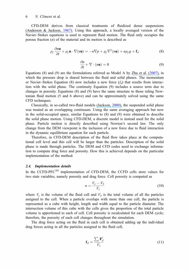
CFD-DEM derives from classical treatments of fluidized dense suspensions(Anderson & Jackson, 1967). Using this approach, a locally averaged version of theNavier–Stokes equations is used to represent fluid motion. The fluid only occupies theporous fraction (n) of the material and its motion is described as

qf@nu@t

þ qf u � rðnuÞ ¼ �nrpþ lfr2ðnuÞ þ nqf g þ fd (8)

@n

@tþr � ðnuÞ ¼ 0 (9)

Equations (8) and (9) are the formulations referred as Model A by Zhu et al. (2007), inwhich the pressure drop is shared between the fluid and solid phases. The momentumor Navier–Stokes Equation (8) now includes a new force (fd) that results from interac-tion with the solid phase. The continuity Equation (9) includes a source term due tochanges in porosity. Equations (8) and (9) have the same structure to those ruling New-tonian fluid motion (5 and 6 above) and can be approximately solved using the sameCFD techniques.

Classically, in so-called two-fluid models (Jackson, 2000), the suspended solid phasewas treated as an overlapping continuum. Using the same averaging approach but nowin the solid-occupied space, similar Equations to (8) and (9) were obtained to describethe solid phase motion. Using CFD-DEM, a discrete model is instead used for the solidphase. Particle motion is directly described using Newton’s second law. The onlychange from the DEM viewpoint is the inclusion of a new force due to fluid interactionin the dynamic equilibrium equation for each particle.

Therefore, in CFD-DEM description of the fluid flow takes place at the computa-tional cell level and this cell will be larger than the particles. Description of the solidphase is made through particles. The DEM and CFD codes need to exchange informa-tion to compute drag force and porosity. How this is achieved depends on the particularimplementation of the method.

2.4. Implementation details

In the CCFD-PFC3D implementation of CFD-DEM, the CCFD cells store values fortwo state variables, namely porosity and drag force. Cell porosity is computed as

n ¼ Ve � Vb

Ve(10)

where Ve is the volume of the fluid cell and Vb is the total volume of all the particlesassigned to the cell. When a particle overlaps with more than one cell, the particle isrepresented as a cube with height, length and width equal to the particle diameter. Theintersection volume of this cube with the cells gives the proportion of the total particlevolume is apportioned to each of cell. Cell porosity is recalculated for each DEM cycle;therefore, the porosity of each cell changes throughout the simulation.

The drag force acting on the fluid in each cell is obtained adding up the individualdrag forces acting in all the particles assigned to the fluid cell,

fd ¼P

j Fjd

Ve(11)

6 N. Climent et al.

where Fjd is the drag force due to the particle j. Particles overlapping several cells share

their force between cells using the ratio used to apportion particle volume.An empirical expression (Wen & Yu, 1966) is used to evaluate the particle drag

force

Fd ¼ 1

2Cdqf pr

2ju� vjðu� vÞ� �

n�v (12)

where Cd is the drag coefficient, u is the fluid velocity, v is the particle velocity, n isthe porosity and χ is a correction factor. The drag coefficient and porosity correction aregiven by the following empirical relationships (Di Felice, 1994).

Cd ¼ :63þ 4:8ffiffiffiffiffiffiffiRep

p!2

(13)

v ¼ 3:7� :65 exp �ð1:5� log10ðRepÞÞ22

!(14)

where Rep is the particle Reynolds number, Equation (15).

Rep ¼2qf rju� vj

lf(15)

In the DEM, the forces due to the presence of the fluid, f fluid are added as an externalforce, Fe

i (Equation (1)), acting on every particle.

f fluid ¼ Fd þ 4

3pr3ðrp� qf gÞ (16)

As shown in Equation (16), the force added has three terms: drag, buoyancy and pres-sure gradient. The drag force is due to the relative particle-fluid velocity and buoyancyis due to the fluid density. Buoyancy is negligible when the fluid considered is a gas,but it must be considered for liquids.

In principle, each fluid cell is sized to contain a statistically significant number ofparticles. The CCFD add-on assumes that the local porosity is evenly distributed withinone cell. Therefore, a sufficiently large number of PFC3D particles should fit inside aCFD cell. Itasca (2008b) suggests that the number of particles be selected by consider-ing the following inequality:

Dxcfd2r

[ 5 (17)

where Δxcfd is the length of the cell and r is the particle radius. Each particle in the cellhas its own velocity, while the fluid velocity is the same for the entire cell. For eachparticle within a given fluid cell, the drag force differs, because it depends on the indi-vidual particle velocity. The buoyancy and pressure forces also vary as they depend onthe particle radii.

During a simulation, the two codes exchange data only at certain times. Thecoupling interval is the time elapsed between data exchanges. During the coupling inter-val, both codes run sequentially using their own time step, different for each one. The

European Journal of Environmental and Civil Engineering 7

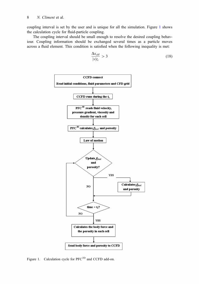
coupling interval is set by the user and is unique for all the simulation. Figure 1 showsthe calculation cycle for fluid-particle coupling.

The coupling interval should be small enough to resolve the desired coupling behav-iour. Coupling information should be exchanged several times as a particle movesacross a fluid element. This condition is satisfied when the following inequality is met:

Dxcfdjvjtc [ 3 (18)

Figure 1. Calculation cycle for PFC3D and CCFD add-on.

8 N. Climent et al.

where tc is the coupling interval and v the particle velocity. (Itasca, 2008b) In practice,the DEM time step is often smaller than the CFD time step. Therefore, several cycles ofDEM are needed to meet one CFD step. The coupling interval chosen in this modelwas 10−5 s.

3. Stress around a cavity: analytical solution

Risnes, Bratli, and Horsrud (1982) studied the stresses around a wellbore by applyingBiot’s theories of poroelasticity and poroplasticity. The well was idealised as a verticalcylindrical hole through a horizontal layer of porous permeable rock. The material wasassumed to be elastic perfectly plastic with a Mohr-Coulomb failure criterion. The fluidflow through the material obeyed Darcy’s law. Axial symmetry and isotropy wereassumed. Deformations and shear failure of the solid skeleton are dependent on theeffective stress which is defined as

r0 ¼ r� a p1 (19)

where r is the total stress tensor, p is the fluid pore pressure, 1 is the unit tensor and αis the Biot parameter given by

a ¼ 1� Kfr=K s (20)

where Kfr is the bulk modulus of the solid skeleton and Ks is the bulk modulus of thesolid grains. For the case of porous sandstones considered here, where sand productionis more likely, α ≈ 1 and the effective stress definition becomes that of Terzaghi.

The geometry assumed in the Risnes et al. model is shown in Figure 2. The sandadjacent to the cavity, bounded by radius Rc behaves plastically and the material outsidethis zone is assumed to behave elastically.

Risnes et al. (1982) derived analytical expressions to estimate the radial, circumfer-ential and vertical total stress in the material as a function of the radial distance fromthe centre of the cavity under steady-state flow conditions (conditions where fluid flowvelocity does not change in time). The analytical solution depends on a number ofmaterial parameters: the Poisson’s ratio (ν), the angle of shearing resistance (frictionangle) of the material (φ), the Biot parameter α, the compressive strength (S0), the per-meability (kc) and the fluid viscosity (μ).

The analytical solution also depends on the boundary conditions, which are theradial total stress at the inner boundary (σri), the vertical total stress at the outer bound-ary (σzo) – from which the radial total stress at the outer boundary (σro) is deducedassuming elastic behaviour – and either the fluid pressure at the outer and inner bound-aries (Po, Pi) or the fluid flow rate (q). The analytical solution is scale-independent: thatis, the only geometric factor affecting the solution is the non-dimensional ratio betweeninner and outer radius.

Figure 3 shows the total and effective radial and circumferential stress distributionsresulting from the analytical solution for different pore pressure levels in a no-flow con-dition (Po = Pi). At the borehole, the effective radial stress is zero. The maximum value(peak) of the circumferential stresses corresponds to the elastic/plastic boundary. Asnoted by Risnes et al. (1982), increasing the pore-pressure resulted in a reduced extentof the plastic zone.

European Journal of Environmental and Civil Engineering 9

4. Model set-up and simulation program

4.1. Model sizing

The model geometry considered in the coupled CFD-DEM simulations is shown inFigure 4(a).

The geometry of this model is one particular case of the Risnes et al. (1982) idealisa-tion. Therefore, the model can be considered to represent a horizontal slice of a confinedvertical cylinder of sandstone with a cylindrical hole in the middle. For given grain size,the computational cost of DEM increases with the cube of model volume. Acceptablecomputing times were obtained with the dimensions shown in the figure; outer radius Ro

of 50 mm, height h of 5 mm and a central cavity with radius Ri of 5 mm.The central cavity radius of the model is far smaller than those typical of producing

wells, but is within the typical range of entrance holes of field perforations in sandstone(Bellarby, 2009). Similar sized holes are also common in laboratory tests designed tostudy the mechanics of sand production (e.g. Ispas, McLennan, & Martin, 2006;Tronvoll, Skjirstein, & Papamichos, 1997; Younessi, Rasouli, & Wu, 2013). The ratiobetween inner and outer radius in the model was selected by considering typical dimen-sions of experimental set-ups.

4.2. DEM specimen

The DEM specimen was formed within two cylindrical walls and two horizontal walls.The discrete material had radii evenly distributed between .4 and .6 mm, which is nearthe upper end of sandstone grain sizes. The specimen was formed with initial porosityof .4, which is larger than that of most reservoir sandstones’. Specimen formationfollowed Cheung (2010): a radius expansion procedure in which small particles, withlinear contacts, seeded within frictionless walls were expanded to attain the target initial

Figure 2. Geometry considered by Risnes et al. (1982).

10 N. Climent et al.

porosity and stress. Then, the parallel bonds were installed; for the simulations pre-sented here all the contacts were bonded, and all the bonds were identical. These bondswere installed to represent the cementation present in the sandstone. The contact param-eters used (Table 1) were proposed by Cheung (2010). After specimen formation, the

Figure 3. Analytical solution: impact of pore pressure, (a) Radial total stress, (b) circumferentialtotal stress, (c) radial effective stress and (d) circumferential effective stress, for different constantpore pressures (0MPa, 30MPa and 60MPa). The radial distance is normalised by the innerradius. Risnes et al. (1982). q = 0 cm3/s; Po = Pi, Ri = .1 m; Ro = 10.0 m; σzo = 65,500 kPa;φ = 30°; So = 101.4 kPa; α = 1.0; and ν = .45.

Figure 4. (a) Model geometry and (b) annular rings created to calculate the continuum stress.

European Journal of Environmental and Civil Engineering 11

wall friction coefficients for the two horizontal platens were changed to .1. No assump-tion of axial symmetry is enforced during specimen formation.

A damping constant δ of .7 was used in all cases. Climent, Arroyo, O’Sullivan, andGens (2013) have shown with a similar model that in “dry” simulations (i.e. DEM with-out fluid) the volume of failed material was very sensitive to the damping value. Moreprecisely, when no damping was applied (δ = 0) the entire specimen failed. The sensitiv-ity to damping disappeared for values higher than .5 for which the results were all quitesimilar. On the other hand in “wet” simulations (where fluid coupling was introduced)the value of this numerical damping had a very small effect on the results. Here bothdry and wet simulations are compared.

During the simulations the inner radial wall was removed and the inner boundarywas transformed into a mass sink, to represent the effect of longitudinal mass transportwithin the cavity. Particles that completely crossed this boundary were thus deleted andconsidered produced. Including this kind of solid granular flow through a boundary isnot a problem for a DEM model, but it does clearly differ from the basic assumptionsunderlying the analysis of Risnes et al. (1982).

4.3. CFD model set-up

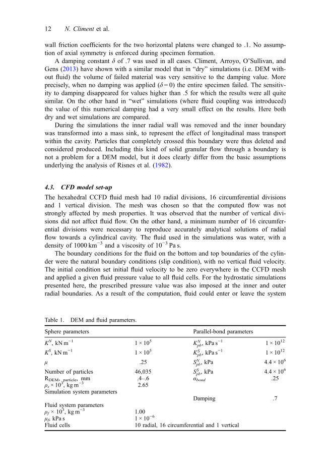
The hexahedral CCFD fluid mesh had 10 radial divisions, 16 circumferential divisionsand 1 vertical division. The mesh was chosen so that the computed flow was notstrongly affected by mesh properties. It was observed that the number of vertical divi-sions did not affect fluid flow. On the other hand, a minimum number of 16 circumfer-ential divisions were necessary to reproduce accurately analytical solutions of radialflow towards a cylindrical cavity. The fluid used in the simulations was water, with adensity of 1000 km−3 and a viscosity of 10−3 Pa s.

The boundary conditions for the fluid on the bottom and top boundaries of the cylin-der were the natural boundary conditions (slip condition), with no vertical fluid velocity.The initial condition set initial fluid velocity to be zero everywhere in the CCFD meshand applied a given fluid pressure value to all fluid cells. For the hydrostatic simulationspresented here, the prescribed pressure value was also imposed at the inner and outerradial boundaries. As a result of the computation, fluid could enter or leave the system

Table 1. DEM and fluid parameters.

Sphere parameters Parallel-bond parameters

KN, kN m−1 1 × 105 KNpb, kPa s

−1 1 × 1012

KS, kN m−1 1 × 105 KSpb, kPa s

−1 1 × 1012

μ .25 SNpb, kPa 4.4 × 106

Number of particles 46,035 SSpb, kPa 4.4 × 106

RDEM, particle, mm .4–.6 αbond .25ρs × 103, kg m−3 2.65Simulation system parameters

Damping .7Fluid system parametersρf × 103, kg m−3 1.00μf, kPa s 1 × 10−6

Fluid cells 10 radial, 16 circumferential and 1 vertical

12 N. Climent et al.

through these pressure-controlled boundaries. The boundary fluid flow will have com-pensated for any overall increase in porosity within the CFD mesh due, for instance, togranular flow (i.e. sand production).

4.4. Simulation program

The material parameters were the same for all the CFD-DEM simulations consideredhere and the simulation program focused on the effect of different stress conditions.These conditions are presented in Table 2.

It should be noted that DEM walls apply effective (intergranular) stresses and nottotal stresses. Fluid pressures, on the other hand, are not directly entered into the DEMmodel, but, as described previously, applied as separate boundary conditions on theCCFD grid.

In all the simulations, the horizontal upper and lower walls of the DEM model arefixed, the external radial wall is used to apply the desired stress level and the internalradial wall is removed. Removing the internal radial wall is equivalent to applying zeroeffective stress at the cavity boundary. As mentioned before, particles that crossed theradial inner boundary during the simulations were deleted and considered “produced”.Referring to the sand production mechanisms introduced in Section 1.1, this model aimsto reproduce both the mechanical failure (that appears as broken inter-particle bonds)and the fluid driven erosion at the cavity boundary (which is represented by the particlesink at the inner radial boundary).

The first three simulations were carried out under a fixed initial vertical total over-burden stress σz0 of 300MPa and varying levels of initial pore pressure p0 (0, 50 and150MPa). As indicated in Table 2, the effective initial stress also varied. The radialeffective stress r0ro that is applied by the external radial wall is computed in each caseas

r0ro ¼ K0r0vo ¼

m1� m

ðrzo � PoÞ (21)

This assumes that the coefficient of at-rest earth pressure K0 is that of an isotropic elas-tic material with Poisson’s ratio ν. This assumption of elastic behaviour at the outerradial boundary follows Risnes et al. (1982). The selection of the Poisson’s ratio valueis explained below.

The initial vertical total stress value used in the first three simulations (300MPa) ishigher than either usual stresses applied in laboratory sand production tests or stressesprevailing in the field. This high value was chosen to ensure that large breakoutsappeared under most scenarios and thus enable full exploration of the the behaviour ofthe model.

Table 2. Simulation program. r0ro is the radial effective stress at the outer boundary and Po isthe fluid pressure at the outer boundary.

Fluid r0ro (MPa) Po (MPa)

SimDry No 300 0Sim50 Yes 200 50Sim150 Yes 120 150Sim300–50 Yes 300 50

European Journal of Environmental and Civil Engineering 13

A fourth simulation was performed in which an effective radial stress of 300MPaand a pore pressure of 50MPa were directly applied. This simulation was carried out toenable a comparison with the first simulation which has the same effective stress level,but has no fluid.

All the simulations were run until a steady state was reached. The term “steadystate” refers here to a situation in which the effective stress variation with radial dis-tance does not vary with time.

5. Results

5.1. Obtaining averaged stresses

A major objective of this work was to compare the simulation results with those derivedfrom the analytical solution of Risnes et al. (1982). The comparison focused on the pro-files of effective stresses such as those in Figure 3. To perform this comparison, it wasnecessary to post-process the simulation results, since contact forces and not stresses arethe basic output DEM variables.

The calculation of the stresses from the DEM data was based on a well-establishedprocedure (O’Sullivan, 2011; Potyondy & Cundall, 2004) in which representative ornotional average stresses are first computed for each grain and then these are averagedin the volume where a representative stress is sought. These stresses are calculated usingonly particle contact forces and are therefore effective stresses.

The averaging volumes used here to compute stresses are the annular rings shownin Figure 4(b). The ring geometry was selected because the analytical Risnes modelassumes axial symmetry, and the p averaged stresses were calculated to enable compari-son with this analytical solution. The width of the rings was selected so that each ringcontained enough number of particles that a statistically significant stress value could becalculated (i.e. a stress value not overly sensitive to the position of one individual parti-cle). Trial and error indicated that 15 rings were enough to ensure proper stress averag-ing, while still capturing most of the radial stress variation.

5.2. Simulation without fluid

A simulation with 0 pore pressure and no fluid (SimDry) was initially performed. Thissimulation plays a key role within the simulation program. The resulting stress distribu-tions were used to calibrate the continuum parameters that enter the Risnes et al. (1982)analytical solution. This means that the analytical solution was evaluated, for the samestress conditions, using different parameter combinations until a good fit was attained.

To achieve this calibration, the sensitivity of the analytical stress distribution to eachinput parameter was established, so they could be adjusted to better fit the numericalresults. The best fit was obtained taking So = 20MPa, φ = 30° and ν = .44. Note that apermeability value was not needed because it plays no role in the analytical solutionwhen the pore pressure is equal at the inner and outer radial boundaries.

The best fit parameter values compare well with values obtained from experimentson sandstones. For example, Alvarado (2007), Alvarado, Coop, and Willson (2012)and Alvarado, Lui, and Coop (2012) studied two sandstones in the laboratory (Castle-gate and Saltwash) and reported a compressive strength that was within 10–30MPa,and a friction angle of around 30°. These parameters are similar to the optimisedparameters. The adjusted value for Poisson’s ratio is a little bit high for a sandstonebut still consistent.

14 N. Climent et al.

Using the adjusted set of continuum parameters, the Risnes et al. (1982) solution islater evaluated at higher pore pressures (50 and 150MPa) and the obtained stress distri-butions compared with the “wet” simulations. Prior to discussing these results in thenext section; the results of this “dry” simulation are considered in detail here.

As fluid is absent this is purely a DEM computation. The comparison with the ana-lytical solution illustrates some interesting aspects of the method. The normalised aver-aged radial and circumferential effective stresses are presented as a function of distanceto cavity in Figure 5, with both the DEM and analytical data being presented. The effec-tive stresses are normalised by the effective stress at the outer boundary and the radialdistance is normalised by the inner radius. The peak of the circumferential effectivestress defines the limit between what Risnes et al. define to be the “plastic” “elastic”zones.

While there is an overall good match between the numerical and the analytical solu-tions for the radial and circumferential effective stresses distributions, there are somenoteworthy differences. There is a decrease in the effective stress near the outer bound-ary for the DEM simulations. This is due to the effect of the rigid cylindrical boundaryon the discrete packing that decreases the porosity and the contacts between particles(Marketos & Bolton, 2010). This effect is also evident in later figures.

The second and most notable difference lies in peak stress values. In Figure 5 peakvalues of the circumferential effective stress differ, with the numerical one being farsmaller. Several reasons might explain this difference. First, the numerical solution (i.e.the steady-state average stress profile) is attained in a dynamical process, whereas theanalytical solution assumes a quasi-static process. Second, in the numerical model solidsmight flow into the cavity; this is not a feature of the analytical model and is accompa-nied by stress relaxation. Third, and perhaps more important, the averaging procedureused to obtain representative stresses from the numerical model has a smoothing effecton the stress data.

Stress – averaging in the DEM model takes place both in the angular and radialdirections. In the radial direction, the resolution of the radial dependency of the stresssolution is limited by the number of annular rings employed (Figure 4). It was observedthat the peak stress value, depended on the number of rings; and when the number ofannular rings decreased the stress values averaged over larger volumes decreasing the

Figure 5. (a) Normalised radial effective stress and (b) normalised circumferential effective stressat the end of SimDry simulation. The results are compared with the analytical solution (Risneset al., 1982). σzo = 300,000 kPa.

European Journal of Environmental and Civil Engineering 15

observed peak value. The peak value in the continuum model is a discrete singularity,stresses for a DEM data-set must be determined over a finite volume, and so this singu-larity cannot be captured exactly.

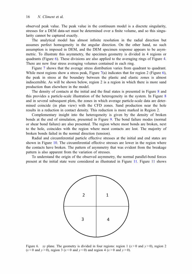
The analytical model has almost infinite resolution in the radial direction butassumes perfect homogeneity in the angular direction. On the other hand, no suchassumption is imposed in DEM, and the DEM specimen response appears to be asym-metric. To illustrate this asymmetry, the specimen geometry is divided in 4 regions orquadrants (Figure 6). These divisions are also applied to the averaging rings of Figure 4.There are now four stress averaging volumes contained in each ring.

Figure 7 shows that the average stress distribution varies from quadrant to quadrant.While most regions show a stress peak, Figure 7(a) indicates that for region 2 (Figure 6),the peak in stress at the boundary between the plastic and elastic zones is almostindiscernible. As will be shown below, region 2 is a region in which there is more sandproduction than elsewhere in the model.

The density of contacts at the initial and the final states is presented in Figure 8 andthis provides a particle-scale illustration of the heterogeneity in the system. In Figure 8and in several subsequent plots, the zones in which average particle-scale data are deter-mined coincide (in plan view) with the CFD zones. Sand production near the holeresults in a reduction in contact density. This reduction is more marked in Region 2.

Complementary insight into the heterogeneity is given by the density of brokenbonds at the end of simulation, presented in Figure 9. The bond failure modes (normalor shear bond failure) are also presented. The region where most bonds are broken, nextto the hole, coincides with the region where most contacts are lost. The majority ofbroken bonds failed in the normal direction (tension).

Radial and circumferential particle effective stresses at the initial and end states areshown in Figure 10. The circumferential effective stresses are lower in the region wherethe contacts have broken. The pattern of asymmetry that was evident from the breakagepattern is also apparent from the variation of stresses.

To understand the origin of the observed asymmetry, the normal parallel-bond forcespresent at the initial state were considered as illustrated in Figure 11. Figure 11 shows

Figure 6. xy plane. The geometry is divided in four regions: region 1 (x > 0 and y > 0), region 2(x < 0 and y > 0), region 3 (x < 0 and y < 0) and region 4 (x > 0 and y > 0).

16 N. Climent et al.

an important asymmetry in the normal parallel-bonds forces at the initial state; there is aregion where forces are mostly compressive (positive) and another region, where forcesare tensile (negative). Where bond forces are initially tensile bonds are easier to breakthan bonds which are in regions where the forces are initially compressive.

Figure 7. Analytical solution and normalised circumferential effective stresses at the end ofSimDry in (a) region 1, (b) region 2, (c) region 3 and (d) region 4.

Figure 8. xy plane. Contact density (number of contact forces per unit cell volume) (a) at the ini-tial state and (b) at the end of SimDry. The outer radius represented is 30 mm.

European Journal of Environmental and Civil Engineering 17

Figure 9. xy plane. (a) Broken bond density (number of broken bonds per cell volume) (b)normal bond failure density (number of normal bond failures per unit cell volume) and (c) shearbond failure density (number of shear bond failures per cell volume) at the end of SimDry. Theouter radius represented is 30 mm.

Figure 10. xy plane. Particle radial effective stresses (a) at the initial state and (b) at the end ofSimDry; particle circumferential effective stresses (c) at the initial state and (d) at the end ofSimDry. The outer radius represented is 30 mm.

18 N. Climent et al.

5.3. Simulations with fluid

Various simulations with fluid under hydrostatic initial conditions (without flow) wereperformed and the results were compared with response predicted by Risnes et al.(1982). All of the simulations were run until the steady state was reached, i.e. when theaverage stress for each ring became constant with time.

Figure 12 compares the circumferential effective stresses obtained in the differentnumerical simulations with those predicted by the Risnes et al. (1982) solution. Intro-ducing fluid in the numerical solution has an effect similar to that which was observedin the analytical solution: the plastic zone radius is reduced in size and larger peakeffective stresses are sustained. However, in the numerical results, the stress peaks arealways less sharp. A likely reason for that difference is the averaging of inhomogeneityon the numerical solution that was discussed before.

In contrast to the previous simulations that have been presented, these simulationsare not pure DEM but coupled DEM-CFD. Fluid flow was indeed observed during thesimulations (see Figure 16(c)–(d) below). Even though the fluid is initially static and themodel boundary conditions are hydrostatic, flow does initiate, because of the localdynamic interaction between the fluid and the particles.

Because the fluid is initially static, grain motion is initially opposed by the fluiddrag force (Equation (12)). Thus, in these simulations, fluid motion is a consequence,and not a cause, of bond breakage and subsequent grain motion. The presence of fluidtherefore has a stabilizing effect.

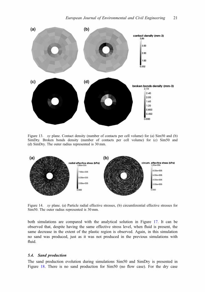
The stabilizing presence of fluid is explored in detail by comparing results forSim50 (results for Sim150 are the same) with results from the dry simulation. To facili-tate the discussion, in this comparison, as before, we use the CFD cells as averagingvolumes for the DEM generated micro variables. Contact densities are thus presented inFigure 13, showing a larger reduction adjacent to the cavity for the dry case(Figure 13(a)). There are also fewer broken contacts in the simulation with fluid(Figure 7(c)). Particle radial and circumferential effective stresses are presented inFigure 14 for the simulations with fluid showing a much reduced low stress zone incomparison with the data presented in Figure 10. Finally, the void ratio next to the holeat the end of SimDry is larger than the void ratio next to the hole at the end of Sim50(Figure 15).

Figure 11. xy plane. Normal bond forces at the initial state. The outer radius represented is 30 mm.

European Journal of Environmental and Civil Engineering 19

Figure 16 presents the drag body force acting on the fluid due to particle motion ineach cell, the fluid flow velocity in each fluid cell and the particle velocity magnitude ineach cell at the beginning of the simulation (when the inner wall has just been removed)and close to the end of the simulation. It is clear that the fluid flow velocities, drag bodyforced and particle velocities have their largest values in the cells where stresses arelowest and most contacts are broken (Figures 13 and 14). At the beginning of the simu-lation, the particles move relatively quickly (Figure 16(e)) and transfer body force to thefluid. These motions are opposed by the fluid and, by the end of the simulation, the par-ticle velocity has reduced by several orders of magnitude, the particles remain in placeand the steady state in terms of average stress is attained.

Because of the raised level of pore pressure, in the “wet” simulations the effectivestresses are lower than in the dry simulation. It might be argued then that the reducedsize of the plastic region and lack of sand production observed in the “wet” simulationsare just a consequence of this reduced effective strength level. To explore that hypothe-sis, a simulation (Sim300–50, Table 2) was performed with the same effective radialstress of 300MPa as the dry simulation but now with the fluid at a hydrostatic initialpore pressure of 50MPa. The circumferential averaged stress distribution results for

Figure 12. Normalised circumferential effective stresses (a) at the end of SimDry, Sim50 andSim150 and (b) the analytical solutions for pore pressures of 0MPa (P = 0), 50MPa (P = 50) and150MPa (P = 150).

20 N. Climent et al.

both simulations are compared with the analytical solution in Figure 17. It can beobserved that, despite having the same effective stress level, when fluid is present, thesame decrease in the extent of the plastic region is observed. Again, in this simulationno sand was produced, just as it was not produced in the previous simulations withfluid.

5.4. Sand production

The sand production evolution during simulations Sim50 and SimDry is presented inFigure 18. There is no sand production for Sim50 (no flow case). For the dry case

Figure 13. xy plane. Contact density (number of contacts per cell volume) for (a) Sim50 and (b)SimDry. Broken bonds density (number of contacts per cell volume) for (c) Sim50 and(d) SimDry. The outer radius represented is 30 mm.

Figure 14. xy plane. (a) Particle radial effective stresses, (b) circumferential effective stresses forSim50. The outer radius represented is 30 mm.

European Journal of Environmental and Civil Engineering 21

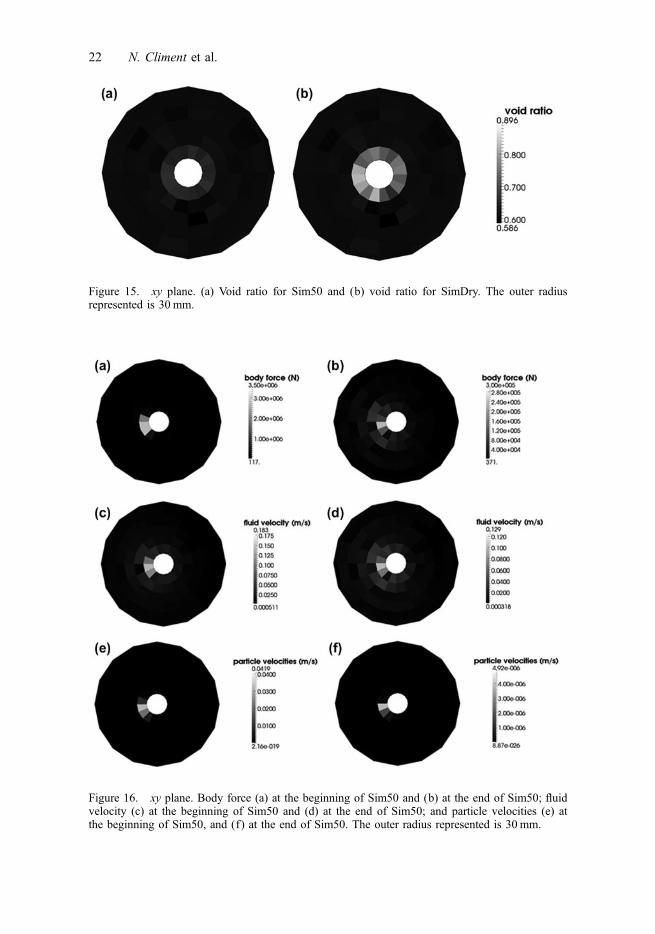
Figure 15. xy plane. (a) Void ratio for Sim50 and (b) void ratio for SimDry. The outer radiusrepresented is 30 mm.

Figure 16. xy plane. Body force (a) at the beginning of Sim50 and (b) at the end of Sim50; fluidvelocity (c) at the beginning of Sim50 and (d) at the end of Sim50; and particle velocities (e) atthe beginning of Sim50, and (f) at the end of Sim50. The outer radius represented is 30 mm.

22 N. Climent et al.

(SimDry), sand production starts at the beginning of the simulation and there is a veryhigh sand production rate. After .01 s, it stabilizes. Sand production is continuous andnot in sudden steps or bursts. Zhou et al. (2011) noted that where sand production wasdriven by a radial fluid flow, sand was produced in clusters or blocks of grains; on theother hand, when no fluid flow was present, sand was produced grain by grain, rathercontinuously. This last observation of Zhou et al. (2011) is in agreement with what hasbeen observed here.

Figure 17. Normalised circumferential effective stress for SimDry and Sim300–50 simulations.(a) Analytical and (b) numerical solutions.

Figure 18. Sand production evolution for Sim50 (represented as ‘no flow’ case) and SimDry.

European Journal of Environmental and Civil Engineering 23

6. Conclusions

A CFD-DEM-coupled model for sand production in sandstone has been presented andapplied to dry and hydrostatic cases. A systematic comparison was made with the pre-dictions of continuum solutions. It is important to note that in the current implementa-tion of the method, only effective stresses can be applied at the boundaries of the DEMmodel, whereas only fluid pressure can be applied in the parallel CFD code.

During dry simulations, a plastic region is created around the borehole. At the mi-cromechanical level, bonds break in that region, particle stresses are reduced, contactsdisappear and sand is produced. Most of the bonds break in the normal (i.e. tensile)mode. Sand is produced in a continuous manner, without steps.

Stress distributions inferred from the numerical solutions are smoothened by averag-ing under the assumption of axial symmetry. Axial symmetry is not present in the initialmicrostate of the sample, where tensile forces in bonds cluster in certain areas. As aconsequence, asymmetric breakouts are produced.

When there is fluid, there is a transfer of momentum between particles and fluid. Inhydrostatic cases, like those examined here, the presence of fluid is stabilizing. The dragforce acts as a damping force, decelerating particle motion towards the cavity andimpeding significant sand production.

AcknowledgementsThe support of the Ministry of Education of Spain through research grant BIA2008-06537 andBIA2011-27217 is gratefully acknowledged. A special thank goes to Dr Jason Furtney of ItascaConsulting Group, Inc. (Minneapolis, Minnesota) for all his help during the implementation of themodel.

ReferencesAlvarado, G. (2007). Influence of late cementation on the behaviour of reservoir sands (PhD the-

sis). University of London, UK.Alvarado, G., Coop, M. R., & Willson, S. (2012). On the role of bond breakage due to unloading

in the behaviour of weak sandstones. Géotechnique, 62, 303–316.Alvarado, G., Lui, N., & Coop, M. R. (2012). Effect of fabric on the behaviour of reservoir sand-

stones. Canadian Geotechnical Journal, 49, 1036–1051.Anderson, T. B., & Jackson, R. (1967). Fluid mechanical description of fluidized beds. Equations

of motion. Industrial and Engineering Chemistry Fundamentals, 6, 527–539.Bellarby, J. (2009). Well completion design, developments in petroleum science (Vol. 56). Oxford:

Elsevier.Boutt, D. F., Cook, B. K., & Williams, J. R. (2011). A coupled fluid-solid model for problems in

geomechanics: Application to sand production. International Journal for Numerical and Ana-lytical Methods in Geomechanics, 35, 997–1018.

Catalano, E., Chareyre, B., & Barthélémy, E. (2013). Pore-scale modeling of fluid-particles inter-action and emerging poromechanical effects. International Journal for Numerical and Analyti-cal Methods in Geomechanics, 38, 51–71.

Cheung, L. Y. G. (2010). Micromechanics of sand production in oil wells (PhD thesis). Universityof London, UK.

Cheung, L. Y. G., O’Sullivan, C., & Coop, M. R. (2013). Discrete element method simulations ofanalogue reservoir sandstones. International Journal of Rock Mechanics and Mining Sciences,63, 93–103.

Climent, N., Arroyo, M., O’Sullivan, C., & Gens, A. (2013). Sensitivity to damping in sand pro-duction DEM-CFD coupled simulations. Powders & Grains. (accepted).

Cook, B. K., Noble, D. R., & Williams, J. R. (2004). A direct simulation method for particle-fluidsystems. Engineering Computations, 21, 151–168.

24 N. Climent et al.

Cundall, P. A. (1987). Distinct element models of rock and soil structure. In E. T. Brown (Ed.),Analytical and computational methods in engineering rock mechanics (pp. 129–163). London:George Allen and Unwin.

Cundall, P. A., & Strack, O. D. L. (1979). A discrete numerical model for granular assemblies.Géotechnique, 29, 47–65.

Di Felice, R. (1994). The voidage function for fluid-particle interaction systems. InternationalJournal of Multiphase Flow, 20, 153–159.

Dorfmann, A., Rothenburg, L., & Bruno, M. S. (1997). Micromechanical modeling of sand pro-duction and arching effects around a cavity. International Journal of Rock Mechanics andMining Sciences, 34, 68.e1–68.e14.

El Shamy, U., & Zeghal, M. (2005). Coupled continuum-discrete model for saturated granularsoils. Journal of Engineering Mechanics, 131, 413.

Ferziger, J. H., & Perić, M. (1999). Computational methods for fluid dynamics (2nd ed.). Berlin:Springer.

Fjær, E., Holt, R. M., Horsrud, P., Raaen, A. M., & Risnes, R. (2008). Stresses around boreholes.Borehole failure criteria. In E. Fjær, R. M. Holt, P. Horsrud, A. M. Raaen, & R. Risnes(Eds.), Petroleum related rock mechanics (pp. 135–174). Oxford: Elsevier.

Grof, Z., Cook, J., Lawrence, C. J., & Štěpánek, F. (2009). The interaction between small clustersof cohesive particles and laminar flow: Coupled DEM/CFD approach. Journal of petroleumscience and engineering, 66, 24–32.

Ispas, I., McLennan, J., & Martin, W. (2006). Interim report on perforation testing for improvedsand management. Technical report. BP and ASRC Energy Services and TerraTek.

Itasca Consulting Group, Inc. (2008a). PFC3D – Particle flow code in 3 dimensions, Ver. 4.0user’s manual. Minneapolis, MN: Itasca.

Itasca Consulting Group, Inc. (2008b). PFC3D – Particle flow code in 3 dimensions, CCFD add-on manual. Minneapolis, MN: Itasca.

Jackson, R. (2000). The dynamics of fluidized particles. Cambridge: Cambridge University Press.Marketos, G., & Bolton, M. (2010). Flat boundaries and their effect on sand testing. International

Journal for Numerical and Analytical Methods in Geomechanics, 34, 821–837.Marrion, M., & Woods, A. (2009). A particle-scale model of hydrodynamic erosion. FMA’09:

Proceedings of the 7th IASME/WSEAS International conference on fluid mechanics and aero-dynamics (pp. 141–149), Corfu.

Nouri, A., Vaziri, H., Kuru, E., & Islam, R. (2006). A comparison of two sanding criteria in phys-ical and numerical modeling of sand production. Journal of petroleum science and engineer-ing, 50, 55–70.

O’Connor, R. M., Torczynski, J. R., Preece, D. S., Klosek, J. T., & Williams, J. R. (1997). Dis-crete element modeling of sand production. International Journal of Rock Mechanics andMining Sciences, 34, 231.e1–231.e15.

O’Sullivan, C. (2011). Particulate discrete element modelling: A geomechanics perspective. Lon-don: Spon Press, Taylor & Francis.

Papamichos, E., & Vardoulakis, I. (2005). Sand erosion with a porosity diffusion law. Computersand Geotechnics, 32, 47–58.

Papamichos, E., Vardoulakis, I., Tronvoll, J., & Skjirstein, A. (2001). Volumetric sand productionmodel and experiment. International Journal for Numerical and Analytical Methods in Geo-mechanics, 25, 789–808.

Potyondy, D. O., & Cundall, P. A. (2004). A bonded-particle model for rock. International Jour-nal of Rock Mechanics and Mining Sciences, 41, 13–29.

Quadros, R., Vargas, E. A., Gonçalves, C. J., & Prestes, A. (2010). Analysis of sand productionprocesses at the pore scale using the discrete element method and lattice Boltzman procedures.Proceedings of the 44th US Rock Mechanics Symposium and 5th U.S.-Canada Rock Mechan-ics Symposium. Salt Lake City, UT.

Rahmati, H., Jafarpour, M., Azadbakht, S., Nouri, A., Vaziri, H., Chan, D., & Xiao, Y. (2013).Review of Sand Production Prediction Models. Journal of Petroleum Engineering, 2013. Arti-cle ID 864981, 16 pages. http://dx.doi.org/10.1155/2013/864981

Risnes, R., Bratli, R. K., & Horsrud, P. (1982). Sand stresses around a wellbore. Society of petro-leum engineers journals. SPE. 9650.

European Journal of Environmental and Civil Engineering 25

Tronvoll, J., Skjirstein, A., & Papamichos, E. (1997). Sand production: Mechanical failure orhydrodynamic erosion? International Journal of Rock Mechanics and Mining Sciences, 34,465.

Tsuji, Y., Kawaguchi, T., & Tanaka, T. (1993). Discrete particle simulation of two-dimensional flu-idized bed. Powder Technology, 77, 79–87.

Wen, C., & Yu, Y. H. (1966). Mechanics of fluidization. Chemical Engineering Progress Sympo-sium Series, 62, 100–111.

Younessi, A., Rasouli, V., & Wu, B. (2013). Sand production simulation under true-triaxial stressconditions. International Journal of Rock Mechanics and Mining Sciences, 61, 130–140.

Zhou, Z. Y., Yu, A. B., & Choi, S. K. (2011). Numerical simulation of the liquid-induced erosionin a weakly bonded sand assembly. Powder Technology, 211, 237–249.

Zhu, H. P., Zhou, Z. Y., Yang, R. Y., & Yu, A. B. (2007). Discrete particle simulation of particu-late systems: Theoretical developments. Chemical Engineering Science, 62, 3378–3396.

26 N. Climent et al.