SEVENTH FRAMEWORK PROGRAMME Theme ICT-2009.1.1 The network of the future Deliverable D2.3 Work Package 2 – System Level Evaluation D2.3Final System Level Evaluation Report Contract no.: 248268 Project acronym: SAMURAI Project full title: Spectrum Aggregation and Multi-user MIMO: Real-World Impact Lead beneficiary: Nokia Siemens Networks Danmark A/S Report preparation date: 31/10/2012 Dissemination level: PU WP2 leader: István Z. Kovács WP2 leader organization: Nokia Siemens Networks Danmark A/S Revision: 1.0

Welcome message from author
This document is posted to help you gain knowledge. Please leave a comment to let me know what you think about it! Share it to your friends and learn new things together.
Transcript
SEVENTH FRAMEWORK PROGRAMME
Theme ICT-2009.1.1
The network of the future
Deliverable D2.3
Work Package 2 – System Level Evaluation D2.3Final System Level Evaluation Report
Contract no.: 248268
Project acronym: SAMURAI Project full title: Spectrum Aggregation and Multi-user MIMO:
Real-World Impact Lead beneficiary: Nokia Siemens Networks Danmark A/S
Report preparation date: 31/10/2012 Dissemination level: PU
WP2 leader: István Z. Kovács WP2 leader organization: Nokia Siemens Networks Danmark A/S
Revision: 1.0

FP7-INFSO-ICT-248268
SAMURAI
10/31/2012 Page 2/75
Contributor list
Name Company Name Company
Hung T. Nguyen, Oscar Tonelli
AAU István Z. Kovács, Mads Brix NSNDA
PéterFazekas Albert Mráz
BME Imran Latif Florian Kaltenberger
EUR
Revision history
Version Authors Comments
V0.1-V0.3
István Z. Kovács PéterFazekas Albert Mráz
Hung T. Nguyen
Early draftToC, May. 2011 First contributions Plan for the contribution, Section
owners and time-plan
V0.4 Imran Latif MIESM based L2SI
V0.5 István Z. Kovács, Oscar Tonelli
ACCS results
V0.6 István Z. Kovács, Mads Brix
SL results for MU-MIMO MIESM Rx and SL results for imperfect CSI
V0.7 Oscar Tonelli, István Z. Kovács,
ACCS results based on ACCSPoC platform experiments
V0.8 Albert Mráz, PéterFazekas inputs on interpolation error modelling
V0.9 Imran Latif changes in section 3
V0.95 Jonathan Duplicy, Michael
Dieudonne
revision of the document
V0.97 PéterFazekas final formatting, editing and harmonization; introductionary parts
V1.0 Michael Dieudonne final check, submission to EC

FP7-INFSO-ICT-248268
SAMURAI
10/31/2012 Page 3/75
EXECUTIVE SUMMARY The SAMURAI project Deliverable D2.3 concludes the system-level studies by incorporating knowledge gained during the development and testing of the
MU-MIMO and ACCS testbeds in Workpackage 5. The studies presented in this deliverable are based on the initial investigation results achieved in Year
1, which have been extended in Year 2 with detailed findings from Workpackage 3, Workpackage 4 and Workpackage 5 studies.
This deliverable presents more in depth investigation and studies done in the last phase of the project, in three main SAMURAI focus areas: i) Effect of
Channel State Information (CSI) measurement and feedback error to the system level performance estimation for downlink (MU-)MIMO; ii) Evaluation of the MIESM based link to system level interface for downlink MU-MIMO and
interference aware receivers, based on findings of Work-package 3, and iii) Final performance evaluation of the proposed Autonomous Component carrier
Selection (ACCS) concept using the SAMURAI ACCS demonstration platform characterises and deployment scenarios.Each section dealing with these areas is a self-contained topic with connections to other Work packages of
the SAMURAI project.
Section 2 contains the latest evaluation and results regarding the interfacing and performance of the interference aware receiver structure developed in WP3. A method is presented that allows the abstraction of this receiver,
hence its performance at system level in realistic circumstances can be and was evaluated. Numerical results of its performance are shown, revealing
that this receiver can bring significant gain in system capacity, at the price of modestly decreasing individual average UE throughput and cell-edge UE throughput performance.
Section 3 is devoted to present the latest findings in the area of modelling
and evaluation of the effect of CSI impairments. Generic framework for CSI errors is shown and is used to simulate system level quality measures when
such errors are present. Further studies on the modelling of the CSI error due to frequency domain interpolation errors are also shown. Numerical results on system level throughput revealed that generally various CSI error
models do not cause significant performance loss.
Section 4 describes the final system level evaluation of the Autonomous Component Carrier Selection (ACCS) method developed in WP4. Throughput performance and spectrum usage of the algorithm, as well as optimisation of
various thresholds and parameters are shown, based on system level simulations conducted in numerous environments. Results of the proof of

FP7-INFSO-ICT-248268
SAMURAI
10/31/2012 Page 4/75
concept platform developed in WP5 are fed back and compared with
simulations.

FP7-INFSO-ICT-248268
SAMURAI
10/31/2012 Page 5/75
DISCLAIMER
The work associated with this report has been carried out in accordance with the highest technical standards
and the SAMURAI partners have endeavoured to achieve the degree of accuracy and reliability appropriate
to the work in question. However since the partners have no control over the use to which the information
contained within the report is to be put by any other party, any other such party shall be deemed to have
satisfied itself as to the suitability and reliability of the information in relation to any particular use, purpose
or application.
Under no circumstances will any of the partners, their servants, employees or agents accept any liability
whatsoever arising out of any error or inaccuracy contained in this report (or any further consolidation,
summary, publication or dissemination of the information contained within this report) and/or the
connected work and disclaim all liability for any loss, damage, expenses, claims or infringement of third
party rights.

FP7-INFSO-ICT-248268
SAMURAI
10/31/2012 Page 6/75
Table of contents
EXECUTIVE SUMMARY ........................................................................... 3 Definitions, symbols and abbreviations ................................................... 10 1 Final WP2 conclusions ..................................................................... 12
1.1 Conclusions on downlink MU-MIMO ............................................. 12
1.2 Conclusions on carrier aggregation ............................................. 14
1.3 Conclusions on joint carrier aggregation and MU-MIMO performance
15
2 Link-to-System interface for Interference Aware receivers .................. 16 2.1 Introduction ............................................................................. 16
2.2 Abstraction for MU-MIMO using EESM ......................................... 17
2.3 Abstraction for MU-MIMO using MIESM ....................................... 18
2.3.1 Modulation Model ................................................................ 18 2.3.2 Coding Model ..................................................................... 20 2.3.3 Calibration of Adjustment Factor ........................................... 21 2.3.4 Results .............................................................................. 21
2.4 System level evaluation results .................................................. 24
2.4.1 Introduction ....................................................................... 24 2.4.2 Results and discussions ....................................................... 25
2.5 Conclusions and practical considerations ..................................... 26
3 Imperfect CSI modelling for downlink MU-MIMO ................................ 28 3.1 Introduction ............................................................................. 28
3.2 Modelling CSI measurement and feedback errors in system level studies ............................................................................................ 28
3.3 Modelling CSI error due to frequency domain interpolation for system level studies ..................................................................................... 31
3.3.1 Basic description of the CSI error model ................................ 31 3.3.2 Simulation assumptions ....................................................... 34 3.3.3 Investigations for different channel models ............................ 34
3.4 System level evaluation results for CSI with interpolation error ...... 37
3.4.1 Introduction ....................................................................... 37 3.4.2 Results and discussions ....................................................... 38
3.5 Conclusions and practical considerations ..................................... 41
4 Autonomous Component Carrier Selection evaluation in real-life scenarios 42
4.1 Introduction ............................................................................. 42
4.2 Scenarios and assumptions ........................................................ 43
4.3 Component carrier selection thresholds ....................................... 47

FP7-INFSO-ICT-248268
SAMURAI
10/31/2012 Page 7/75
4.3.1 High transmit power (20 dBm) ............................................. 47 4.3.2 Low transmit power(0 dBm) ................................................. 47 4.3.3 Conclusions on BCC-SCC selection thresholds ......................... 52
4.4 Inter-eNB path loss ranging threshold selection ........................... 53
4.4.1 Conclusions on path loss ranging threshold selection ............... 55 4.5 Resource utilization performance ................................................ 55
4.5.1 Deployment scenario with 6 cells .......................................... 55 4.5.2 Deployment scenario with 4 cells .......................................... 58
4.6 ACCS on the demonstrator testbed .................................................. 61
4.6.1 ACCS performance comparison with simulations ..................... 62 4.6.2 Analysis of C/I thresholds in a dynamic environment ............... 64 4.6.3 ACCS performance in comparison to reuse 1 ................................. 65
4.7 Conclusions and practical considerations ........................................... 67
4.7.1 Main findings and recommendations ...................................... 67 References ......................................................................................... 69 5 Appendices ................................................................................... 71
5.1 Appendix A Frequency domain interpolation errors for several ITU multipath profiles ............................................................................. 71
Table of figures
Figure 2-1 Abstraction in System Performance Evaluation ......................... 17 Figure 2-2 Mutual Information based abstraction model ........................... 19 Figure 2-3 MI as a function of desired signal and interfering signal strength 20 Figure 2-4RBIR Vs. SINR ...................................................................... 21 Figure 2-5 EESM Link Abstraction for IA Receiver with two calibration factors
......................................................................................................... 23 Figure 2-6 MIESM-M1 Link Abstraction for IA Receiver with only one calibration factor ................................................................................. 24 Figure 2-7 System-level performance metrics from the MU-MIMO IA receiver evaluation studies. .............................................................................. 26 Figure 2-8 System-level cell throughput versus Geometry factor from the MU-MIMO IA receiver evaluation studies. ................................................ 26 Figure 3-1 The developed system-level modelling framework for the CSI
measurement and feedback error. ......................................................... 30 Figure 3-2 Illustration of the channel equalization with the actual and the
estimated channel. .............................................................................. 32 Figure 3-3 Illustration of the frequency-domain interpolation. ................... 33 Figure 3-4 Average squared estimation error in different ITU channels. ...... 35 Figure 3-5 Frequency domain interpolation error for ITU Ped. A................. 36 Figure 3-6 Frequency domain interpolation error for ITU Veh. A. ............... 37 Figure 3-7 System-level performance from the CSI/CQI error model evaluation studies. .............................................................................. 39

FP7-INFSO-ICT-248268
SAMURAI
10/31/2012 Page 8/75
Figure 3-8 Outer Loop Link Adaptation CQI offset distribution from the CSI
error modelling evaluation studies when using SU-MIMO transmission scheme. ............................................................................................. 40 Figure 3-9 Outer Loop Link Adaptation CQI offset distribution from the CSI
error modelling evaluation studies when using SU/MU-MIMO transmission scheme. ............................................................................................. 40 Figure 4-1 ACCS PoC measurement layout used to derive deployment scenarios for the system-level studies. ................................................... 44 Figure 4-2 Example of “6-room” A0 and “4-room” A5 deployment scenarios
with UEs in the same room as the serving eNBs (TX=eNB, RX=UE). .......... 44 Figure 4-3 Example of “4-room” A3 deployment scenario with two UEs in
different room than the serving eNBs (TX=eNB, RX=UE). ......................... 45 Figure 4-4 Average ACCS downlink UE throughput performance in low offered traffic load conditions, with 20dBm eNB Tx power, versus the
CoI_Target_BCC and CoI_Target_SCC parameter combinations. See Table 4-3 for the x-axis legend. ..................................................................... 48 Figure 4-5 Average ACCS downlink UE throughput performance in high offered traffic load conditions, with 20dBm eNB Tx power, versus the
CoI_Target_BCC and CoI_Target_SCC parameter combinations. See Table 4-3 for the x-axis legend. ..................................................................... 49 Figure 4-6 Average ACCS downlink UE throughput performance in low offered
traffic load conditions, with 0dBm eNB Tx power, versus the CoI_Target_BCC and CoI_Target_SCC parameter combinations. See Table 4-3 for the x-axis
legend. .............................................................................................. 50 Figure 4-7 Average ACCS downlink UE throughput performance in high offered traffic load conditions, with 0dBm eNB Tx power, versus the
CoI_Target_BCC and CoI_Target_SCC parameter combinations. See Table 4-3 for the x-axis legend. ..................................................................... 51 Figure 4-8 Average ACCS downlink UE throughput performance in increasing traffic load conditions, versus PLThreshold and transmit power settings. See Table 4-4 for the x-axis legend.............................................................. 54 Figure 4-9 Average spectral resource utilization (number of CCs) in the deployment scenarios A0-A2 for low and high traffic load conditions. ......... 56 Figure 4-10 Examples of average spectral resource sharing (fraction of shared CC resources) for each eNB pair, in the deployment scenario A0 for low and high traffic load conditions. ....................................................... 57 Figure 4-11 Examples of spectral resource sharing (fraction of shared CC resources) realization versus time, in the deployment scenario A0 for low and
high traffic load conditions. ................................................................... 58 Figure 4-12 Average spectral resource utilization (number of CCs) in the deployment scenarios A5-A7 for low and high traffic load conditions. ......... 59 Figure 4-13 Examples of average spectral resource sharing (fraction of shared CC resources) for each eNB pair, in the deployment scenario A5 for
low and high traffic load conditions. ....................................................... 60

FP7-INFSO-ICT-248268
SAMURAI
10/31/2012 Page 9/75
Figure 4-14 Examples of spectral resource sharing (fraction of shared CC
resources) realization versus time, in the deployment scenario A5 for low and high traffic load conditions. ................................................................... 61 Figure 4-15 Cumulative Distribution Functions of UE DL SINR in the cells in
low traffic conditions (lambda=0.1) and high traffic conditions (lambda = 1) ......................................................................................................... 63 Figure 4-16 Cumulative Distribution Functions of UE DL Throughput in the cells in low traffic conditions (lambda=0.1) and high traffic conditions (lambda = 1) ...................................................................................... 64 Figure 4-17 Time Snapshot of the Carrier to Interference variations in Cell 1 during an experimental run. In the Figure the values for different
environment conditions are reported. ..................................................... 65 Figure 4-18 Cumulative Distribution Functions of UE DL Throughput in the cells for ACCS and REUSE 1 schemes. Dynamic Environment experimental
results have been compared to the Hybrid Simulation. ............................. 66 Figure 5-1 Frequency domain interpolation error for ITU Indoor A. ............ 71 Figure 5-2 Frequency domain interpolation error for ITU Indoor B. ............ 72 Figure 5-3 Frequency domain interpolation error for ITU PedestrianB. ........ 74 Figure 5-4 Frequency domain interpolation error for ITU PedestrianB. ........ 75

FP7-INFSO-ICT-248268
SAMURAI
10/31/2012 Page 10/75
Definitions, symbols and abbreviations
3GPP Third Generation Partnership Project
ACCS Autonomous Component Carrier Selection
AMC Adaptive Modulation and Coding
ARQ Automatic Retransmission reQuest
AWGN Additive White Gaussian Noise
BC Base Carrier
BCC Base Component Carrier
BLER Block-Error-Rate
BS Base Station
CA Carrier Aggregation
CC Component Carrier
cdf cumulative distribution function
C/I Carrier/Interference
CoI Carrier over Interference
CQI Channel Quality Indicator
CSI Channel State Information
DL Downlink
EESM Exponential Effective SINR Mapping
EGT Equal Gain Transmission
eNB Evolved NodeB (E-UTRAN NB/BS)
ESM Effective SINR Mapping
G-factor geometry factor
HARQ Hybrid ARQ
IA receiver Interference Aware receiver
L2S(I) Link-to-System (Interface)
LA Link Adaptation
LTE Long Term Evolution of UTRA(N)
LTE-A Advanced Long Term Evolution of UTRA(N)
MCS Modulation and Coding Scheme
MIESM Mutual Information Effective SINR Mapping
MIMO Multiple Input Multiple Output
MMSE Minimum Mean Square Error
MSE Mean Square Error
MU Multi User
MU-MIMO Multi User MIMO
MUI Multi User interference
OFDM Orthogonal Frequency Division Multiplexing
OLLA Outer Loop Link Adaptation
PMI Precoding Matrix Indicator
PoC Proof-of-Concept

FP7-INFSO-ICT-248268
SAMURAI
10/31/2012 Page 11/75
PRB Physical Resource Block
PS Packet Scheduling
PSK Phase Shift Keying
QAM Quadrature Amplitude Modulation
QPSK Quaternary PSK
RBIR Received Bit Information Rate
RRM Radio Resource Management
Rx Receiver
SC Supplementary Carrier
SCC Supplementary Component Carrier
SI Symbol Information
SINR Signal to Interference plus Noise Ratio
SINReff Effective SINR (compressed SINR as output from L2S)
SU Single User
SU-MIMO Single User MIMO
TTI Transmission Time Interval
Tx Transmitter
UE User Equipment
UL Uplink

FP7-INFSO-ICT-248268
SAMURAI
10/31/2012 Page 12/75
1 Final WP2 conclusions During the course of the project WP2 conducted several activities and achieved significant results (which are reported in previous deliverables D2.1 [1], D2.2 [2] and the current document) in the following areas:
Applicability and performance of several downlink MU-MIMO receiver algorithms at system level
Interfacing (in terms of block error ratio versus SNR)of a novel interference aware MU-MIMO receiver algorithm (developed in WP3) to system level simulator and evaluation of its performance at system
level Analys and modelling several channel estimation errors (interpolation,
quantisation, Gaussian) and providing insights into the downlink system level performance loss during reception, due to the imperfect channel knowledge
Develop models for channel state estimation and feedback errors (delays, losses) and detailed simulation evaluation of their impact on
system level performance in case of MU-MIMO transmission Evaluation of feedback compression schemes applicable for LTE-A
carrier aggregation schemes in order to reduce feedback overhead
System level evaluation of downlink MU-MIMO scheduling algorithms in terms of user throughput cdfs and average cell throughputs
Evaluation of the throughput performance of downlink carrier aggregation schemes with 2x2 SU-MIMO transmission, with focus on the performance gain of LTE-A features
Evaluation of the throughput performance of downlink carrier aggregation schemes applied in combination with MU-MIMO
transmission Evaluation of physical layer enhancement techniques for LTE-Advanced
for uplink carrier aggregation, uplink multi-cluster scheduling and
uplink MU-MIMO transmission Development and system level evaluation of Autonomous Component
Carrier selection mechanisms including methods for selecting Base Carrier and Supplementary Carrier, mainly applicable for dense indoor
Home eNodeB (femtocell) environments, or dense heterogeneous macro/pico network deployment.
1.1 Conclusions on downlink MU-MIMO
Regarding packet scheduling and link adaptation for MU-MIMO in 3GPP LTE Release 8, our studies in deliverable D2.1 [1]show that the optimal spatial
scheduling of the paired UEs and the associated link-adaptation based on the limited channel information feedback available from the UEs is a challenging
task. With baseline assumptions only minimal system performance gain of MU-MIMO can be obtained, compared to SU-MIMO. However, when including

FP7-INFSO-ICT-248268
SAMURAI
10/31/2012 Page 13/75
improved UE receiver algorithm, the system performance can be increased to
approximately 3% to 10% compared to the SU-MIMO reference. The performance of downlink MU-MIMO system can be much enhanced when
LTE-Advanced specific demodulation reference symbols are used. When applying a modified UE selection, pairing and scheduling algorithm proposed
in deliverable D2.2 [2], it is possible to achieve a gain in the average cell-throughput in the order of 23%. Moreover, downlink MU-MIMO transmission technique also improves the performance of cell edge UEs with a potential
gain of 7% as compared with the case they are operating in SU-MIMO transmission mode.
Considering different impairments in the estimation and reporting of the channel state information, our studies in deliverable D2.1 show that feedback
delay may cause around 5 dB loss in the block error ratio (BLER) performance even for advanced receiver architectures. Channel estimation
errors due to quantisation cause negligible performance loss, also estimation error due to interpolation stays in the regime of 1-2 dB in the BLER
performance. The effect of PMI loss on the performance also stays at the tolerable level, when considering reasonably low loss probability of the PMI. In the deliverable D2.2 we show that MU-MIMO CQI estimation can be
effectively enhanced by advanced methods, compared to the traditional fixed CQI offset approach and this can lead to an 8% improvement in average cell
throughput. Our results have also shown that MU-MIMO CQI estimation based on adaptive rank shows near a constant throughput and outperforms rank-1 MU-MIMO CQI prediction significantly when SNR increases. Even
adaptive rank CQI prediction requires more feedback, less precoding operations and easier channel estimations at UE is required and as such is
more robust and practicable for LTE systems beyond Release8. The unified framework of modelling different channel estimation errors lead
to system-level results that show little impact of the various CSI/ CQI error models in case of rank-adaptive SU-MIMO transmission, with at most 2.5%
and 4.5% degradation for the average UE throughput and cell-edge (5%-ile) UE throughput levels, respectively. As a general rule, and as expected, the highest impact from CSI/CQI errors for vehicular channels estimation errors,
while with the pedestrian channel estimation errors (3 kmph) there is no significant performance degradation visible.
With regards to interfacing the novel interference aware receiver developed in WP3 into the system level simulator of WP2, we may conclude that the
accurate mutual information based effective SINR mapping (MIESM) method is very effectively replaced by exponential effective SINR mapping (EESM)
with two calibration factors. Using this interfacing method, system level

FP7-INFSO-ICT-248268
SAMURAI
10/31/2012 Page 14/75
results in this deliverable D2.3 show that IA receiver based MU-MIMO
scheme can provide 20% gain in cell capacity compared to SU-MIMO.
1.2 Conclusions on carrier aggregation
Regarding feedback compression, three main extensions of feedback schemes have been proposed and evaluated under bursty traffic conditions. The results presented in deliverable D2.1 [1] show the optimal trade-off
between feedback size and the system performance is obtained when using the Average Best-M CQI (UE selected) and Wideband PMI type of feedback in
each active component carrier. Regarding carrier aggregation throughput performance, it is shown in
deliverable D2.1 that for full buffer traffic load, LTE-Advanced UEs can provide up to 23% average cell throughput increase compared to the
performance with LTE Release 8 UEs only. The gain in UE throughput is dependent on the component carrier settings and the highest gains are observed in the 4x10 MHz setting with 40% and 27% in the median and cell-
edge UE goodput respectively. For finite buffer and bursty traffic the performance gains of CA system over a single component carrier vary
according to the load conditions. At low load, the average goodput of the UEs in a CA system can be N times (N is the number of aggregated carriers) higher that of the UEs in a traditional single component carrier. The gain of
the CA system gradually degrades from low to medium cell load conditions. At very high cell load the gain of the CA system becomes negligible in terms
of UE goodput.
In the area of Autonomous Component Carrier Selection (ACCS) it can be concluded that there is a clear gain from using a relatively simple, matrix based initial base component carrier (BCC) selection algorithm compared to a
pure random BCC selection [1]. Furthermore, this algorithm needs to be extended with supplementary component carrier (SCC) selection algorithm
for optimal carrier configuration. In medium to high load scenarios, a system configuration with at least three CCs can fully benefit from the proposed ACCS interference mitigation scheme, while the required signalling
complexity and overhead are kept to minimum. In large scale deployments the acceptable path-loss detection threshold between the Femto-eNBs
(PLThreshold) is in the range of 102-140dB. In smaller deployment scenarios the acceptable PLThreshold can be lower in the range of 80-90dB. For the effective operation of the ACCS algorithm the {BCC, SCC} selection carrier
over interference (C/I) thresholds combinations should be set in the range of {20, 8 to 11} dB for deployments with at least 6 neighbouring cells, while
the range of {17, 5 to 11} dB can be used for smaller number of neighbouring cells, and regardless of the cell total downlink transmit power. System level studies show that in terms of UE throughput, ACCS performs

FP7-INFSO-ICT-248268
SAMURAI
10/31/2012 Page 15/75
well in situation of high traffic load and high interference coupling between
the cells [1][2]. In this deliverable D2.3, experimental and simulation studies have been conducted and documented when using practical ACCS PoC deployment scenarios [10]. In these real-life deployment scenarios, including
dynamic radio channel conditions, it was shown that further optimization, and possibly also an adaptation mechanism, is needed in order to set the
correct C/I threshold values used in the component carrier selection.
1.3 Conclusions on joint carrier aggregation and MU-MIMO performance
In the downlink studies with CA and SU/MU-MIMO, under full buffer load traffic assumptions the MU-MIMO transmission performed better than the
SU-MIMO transmission. This result is expected and similar to the non-CA results. However, in practical traffic load conditions (finite buffer with bursty traffic), it was shown in deliverable D2.2 [2] that MU-MIMO yields
performance enhancement in terms of UE goodput only in high traffic load conditions. It is highlighted that MU-MIMO techniques can only obtain gain
when there are numerous UEs and the system can exploit the multi-user diversity gain. Due to the characteristic of the bursty traffic, the gain achieved with MU-MIMO transmission is amplified and the overall
performance enhancement is much larger than the gain obtained in full buffer traffic load conditions (up to 20% gain compared to CA with SU-
MIMO). In uplink direction, when carrier aggregation and MU-MIMO are both
deployed, several physical layer enhancement techniques were presented in deliverable D2.2 and shown to yield significant performance increase. It is
shown that with proper separation between power-limited and non-power-limited LTE-A users, multi-cluster scheduling with CA has similar coverage performance as in LTE Release 8, but can achieve substantial gains, up to
56%, in average user throughput compared with LTE Release 8. Uplink MU-MIMO can further improve the throughput performance, especially when MU-
MIMO is combined with multi-cluster scheduling.

FP7-INFSO-ICT-248268
SAMURAI
10/31/2012 Page 16/75
2 Link-to-System interface for Interference Aware receivers
2.1 Introduction
LTE transmission mode 5 precoders are characterized by their low resolution and the principle of equal gain transmission (EGT). Therefore, even with
optimal scheduling the residual MU interference is significant in this transmission mode and can lead to a degradation of the system performance.
A promising way to recover the gains of MU-MIMO in this mode is to employ interference aware (IA) receivers, such as in [15].
Interference aware receivers benefit from the fact that the interfering signal belongs to a finite QAM constellation and has certain structure which can be
exploited during the detection of the desired signal. In other words the interference is not considered as Gaussian in these kinds of receivers.
Link-to-system interfacing or link abstraction models are of utmost importance for large scale system level simulations where these models not
only provide the accurate mapping between link level and system level simulations but can also be used for fast resource scheduling at the eNodeB.
State-of-the-art link abstraction schemes are all post processed SINR based schemes. The most popular basic scheme is the effective SINR mapping
(ESM) where at first the varying SINRs of a codeword are compressed and mapped to an effective SINR value which is then used to read the equivalent
BLER from the AWGN performance curves of a particular modulation and code scheme (MCS).
[
∑ (
)
] (2.1)
( ) (2.2)
where J is the number of channel symbols in a codeword and I( ) is a
mapping function which transforms SINR of each channel symbol to some
“information measure” where itis linearly averaged over the codeword. Then
these averaged values are transformed back to SNR domain. is called
calibration factor and it is there to compensate for the performance of different modulation orders and the code rates.
Figure 2-1 shows the generalized link abstraction methodology for system
level evaluations. System level simulator generates a multi-state channel vector in which each entry corresponds to a subcarrier. Then it calculates the

FP7-INFSO-ICT-248268
SAMURAI
10/31/2012 Page 17/75
post processed SINR values for each of the subcarrier and pass this
information to the link abstraction module where an effective SINR is calculated. Then this effective SINR is mapped onto a link quality metric for example BLER.
ESM can be applied for the linear receivers but for non-linear receiver, i.e.,
interference aware receiver, it cannot be applied directly. The main reason is that for the case of interference aware receiver, we do not know the post-processed SINR values so we need to extend the ESM in such a manner that
it can be used for those kind of receivers where the knowledge of post processed SINR is not available.
There are two widely used ESM techniques for the link abstraction, expected effective SINR mapping (EESM) and mutual-information based effective SINR
mapping (MIESM). In the following we shall describe how these link abstraction techniques can be used for interference aware receiver.
Figure 2-1 Abstraction in System Performance Evaluation
In order to evaluate the abstraction methodology we carried out link-level
simulations using EESM and MIESM and we proposed a new modulation model for the MIESM which is able to exploit the structure of interference.
2.2 Abstraction for MU-MIMO using EESM
EESM is based on post processed SINR for each of the subcarrier and for the
non-linear receiver structures, post processed SINR is not available. However, based on the knowledge of desired user's channel, precoder, noise variance and interfering user's channel, precoder it is possible to calculate
signal-to-interference plus noise ratio. For EESM [1] the mapping function I( ) is calculated using Chernoff Union bound of error probabilities, i.e., I( )
= 1- exp(- ), then effective SINR is calculated as,

FP7-INFSO-ICT-248268
SAMURAI
10/31/2012 Page 18/75
[
∑ (
)
] (2.3)
and based on this effective SINR, then the link quality indicator (BLER) is
computed from previously calculated AWGN performance curves.
( ) ( ) (2.4)
Where is the vector of the SINR values across all of the subcarriers. But
this not an accurate performance metric for modeling the performance of
non-linear receiver structures and it is expected to see a performance loss if it is to be used for link abstraction. This was in fact shown in [2] that using
EESM as described is not able to model the performance of interference aware receiver. Therefore, we decided to investigate the MI based approach.
2.3 Abstraction for MU-MIMO using MIESM
We present an extension of the mutual information based abstraction
methodology for the link abstraction of interference aware receivers and normal receivers. The abstraction model consists of two blocks, modulation model and coding model as shown in Figure 2-2. The inputs for the
abstraction can be SINR values for each subcarrier or the channel of desired user, precoder and constellation of desired and interfering user. Based on the
preferred input the modulation model calculates maximum channel capacity in terms of symbol information for every subcarrier. The modulation model only accounts for the modulator and demodulator. Then in the coding model
symbol information of each subcarrier belonging to the same codeword is averaged over total number of transmitted bits during that codeword to
reach the received bit information rate (RBIR). This RBIR is used to read the effective SNR from SNR-to-normalized SI (symbol information) mapping. Then finally this effective SNR is used to read the BLER from previously
calculated AWGN performance curves corresponding to the specific MCS.
2.3.1 Modulation Model
Modulation model as shown in Figure 2-2 provides us with the symbol
information (SI) in terms of maximum channel capacity for each of the subcarrier. In this deliverable we propose a new modulation model for the specific case of MU-MIMO.

FP7-INFSO-ICT-248268
SAMURAI
10/31/2012 Page 19/75
Figure 2-2 Mutual Information based abstraction model
The proposed modulation model is based on:
( | , )
∑ ∑ ∑ ∑
∑ ∑ [
|
|
]
∑ [
|
| ]
(2.5)
from[14] and is stored in the form of a look up table. This table is a function of the modulation order of the desired stream (M1) and the interfering
stream (M2), the signal to noise ratio (SNR) of the desired stream, desired
signal and interference | |. Since the purpose of link abstraction is to
reduce complexity so table for symbol information mapping should be available as a look-up. To generate these tables we performed Monte-Carlo
simulations of (6) in [14] over a wide range of noise and channel realizations.
For each channel realization we obtained a random set of , | | and mutual information. For all other required values this scatter-plot was interpolated
using linear interpolation. As an example an interpolated graph for the SNR of 10 dB is shown in Figure 2-3 where on the x-axis is the signal strength, on
y-axis is the interference strength and on z-axis is the mutual information.

FP7-INFSO-ICT-248268
SAMURAI
10/31/2012 Page 20/75
Figure 2-3 MI as a function of desired signal and interfering signal strength
2.3.2 Coding Model
The coding model corresponds to the encoding and decoding of the codeword and predicts the performance for whole codeword. The output of modulation
model is a vector of symbol information for all of the subcarriers of a codeword. The first thing which coding model calculates is the collection of received coded bit information (RBI) for the desired user among J subcarriers,
∑ (‖ ‖ ‖ ‖ )
(2.6)
where the first index in modulation order represents the user and second
index represents the subcarrier. is an adjusting factor which compensates of practical coding loss. The optimal value of beta can be trained over a set of
enough channel realizations that covers a reasonable amount of different channel variations.
RBI is then normalized by the number of total coded bits to the received bit information rate (RBIR):
∑
(2.7)

FP7-INFSO-ICT-248268
SAMURAI
10/31/2012 Page 21/75
Figure 2-4RBIR Vs. SINR
As is shown in Figure 2-4, RBIR can also be regarded as normalized SI and is
used for calculating the effective SINR. The normalized symbol information is based on the normalized mutual information expressions for finite
constellation. Then this effective SINR is used to obtain BLER from the equivalent AWGN performance curve for a specific MCS. These AWGN curves are pre-calculated for all MCS of LTE and stored in the form of a look-up
table.
2.3.3 Calibration of Adjustment Factor
Calibration of adjustment factor ( ) is very important forthe accurate mapping of multi-state channels into one-statechannel. We performed
calibration through an iterative procedurewhich requires a starting point
(normally initial = 1)then it is chosen such that,
[∑ | ( ) |
] (2.8)
where Nc is the number of different channel realizations ,BLERpred,mcs is the predicted block error rate from the respective AWGN curve which we
calculated beforehand from the simulator and BLERmeas,mcs is the error rate from Nc channel realizations.
2.3.4 Results
We already presented the results of MU-MIMO abstraction for IA-Receiver
using EESM and two variants of MIESM with one calibration factor in the
FP7-INFSO-ICT-248268
SAMURAI
10/31/2012 Page 22/75
deliverable D2.2 [2] and we showed that MIESM with proposed changes is
the best method for interference aware receiver. However, for its validation on the system level simulator it was required to implement it from the scratch and due to the time constraint, it was not possible. So we invested
some more time in order to find an agreement between EESM (which is already implemented in our system level simulators) and proposed MIESM so
that both can be used interchangeably. Further investigation led us to the conclusion that if two different calibration factors are used in the process of EESM instead of one calibration factor then EESM can reach very close to the
accuracy of proposed MIESM where we use only one calibration factor. This is shown in Figure 2-5 and Figure 2-6.
Figure 2-5 and Figure 2-6 presents the results of MU-MIMO abstraction for MCS 10, 12, 14 and 16 using EESM and MIESM respectively. Please note that
EESM used two calibration factors, whereas MIESM only used one calibration factor. The solid magenta lines in the figure represent the respective AWGN
curves and the coloured stars around solid curves represent the BLER points which are measured using link level simulations for many number of different
channel realizations. As can be seen from the figure that EESM with two calibration factors is able to compress and map the different realizations of MU-MIMO channel onto the respective AWGN curves.

FP7-INFSO-ICT-248268
SAMURAI
10/31/2012 Page 23/75
Figure 2-5 EESM Link Abstraction for IA Receiver with two calibration
factors

FP7-INFSO-ICT-248268
SAMURAI
10/31/2012 Page 24/75
Figure 2-6 MIESM-M1 Link Abstraction for IA Receiver with only one
calibration factor
Therefore, based on the presented results MIESM IA link abstraction was approximated by EESM with two calibration factors. During the derivation of following system level results this method was used and hence referred as
MIESM IA link abstraction.
2.4 System level evaluation results
2.4.1 Introduction
The link-to-system interface developed in Work package 3 and Work package
5 as presented in Section 2.2 and Section 2.3 has been used in downlink system-level evaluations following the procedure described in the previous
Deliverables D2.1 and D2.2 [1][2]. The goal of these studies was to disclose the potential system-level gain
which can be obtained when IA receivers are used for MU-MIMO reception compared to the rank-adaptive SU-MIMO transmission references. The
reader should note that these studies did not aim to show absolute system

FP7-INFSO-ICT-248268
SAMURAI
10/31/2012 Page 25/75
performance numbers or to investigate SU-MIMO performance, as compared
to the reference 3GPP LTE/LTE-A MIMO evaluation studies. The system-level simulations settings, parameters and scheduling algorithm
used can be found it the above referenced documents. A downlink 2x2 MIMO transmission setup was used with 10MHz system bandwidth at 2 GHz carrier
frequency. The 3GPP typical urban deployment and ITU based geometric channel model were employed. The main difference compared to the previous studies was due to the limitation of the available link-to-system
interface mapping curves, which included only QPSK and 16QAM modulation and coding sets. Therefore, to provide a fair comparison, we have used the
same QPSK and 16QAM MCS sets in all simulations presented in the following.All UE terminals simulated are assumed to have the same MIMO capability and implement the IA receiver algorithm. Furthermore, in these
evaluations only the full buffer traffic model (UE download data continuously) has been used in order to have sufficient user diversity in the system (see
Deliverables D2.2 [2]).
The three simulation sets to be compared are: 1. “MU-MIMO Ideal IA”: Rank-adaptive SU-MIMO combined with rank-
1 MU-MIMO using ideal IA receiver (zero residual MU interference at
UE), and ideal MU-MIMO CQI compensation at the eNB 2. “MU-MIMO MIESM-IA”: Rank-adaptive SU-MIMO combined with
rank-1 MU-MIMO using realistic IA receiver, based on the MIESM L2SI curves, and ideal CQI compensation at the eNB
3. “SU-MIMO”: Rank-adaptive SU-MIMO
2.4.2 Results and discussions
Figure 2-7 shows the main system level performance metrics obtained from the MU-MIMO IA evaluations along with the reference SU-MIMO results, in
terms of average cell throughput and UE throughput statistics. Compared to the ideal case of using ideal MU IA (zero residual MU
interference at the UE) the results for the MIESM-IA show very good performance and only 3% degradation; the MIESM IA yields an overall cell
throughput gain of approximately 20% compared to reference SU-MIMO transmission case. Furthermore, looking at the UE throughput statistics, it is clear that this gain comes at the cost of sacrificing the cell-edge performance,
with a loss of approximately 35% compared to the SU-MIMO case.
Figure 2-8 shows more in-sight into the cell throughput gain mechanisms in these studies, in terms of the achieved system throughput vs. geometry factor. It is evident from these results that MU-MIMO transmission schemes
can take advantage of the high G-factor (good SINR conditions at the UE)

FP7-INFSO-ICT-248268
SAMURAI
10/31/2012 Page 26/75
hence improves the overall system spectral efficiency. A second observation
is that UEs in low-medium G-factor conditions are better scheduled in SU-MIMO mode due to the rank-adaptation.
Figure 2-7 System-level performance metrics from the MU-MIMO IA receiver
evaluation studies.
Figure 2-8 System-level cell throughput versus Geometry factor from the
MU-MIMO IA receiver evaluation studies.
2.5 Conclusions and practical considerations
The performed system level simulation studies using IA receiver have
revealed the following main findings to be considered in practical deployments:
1. The user diversity order has to be relatively high in given cell in order to be able to take advantage of the MU-MIMO transmission scheme.
MU-MIMO Ideal IA MU-MIMO MIESM-IA SU-MIMO0
2000
4000
6000
8000
10000
12000
14000
16000
Avera
ge c
ell
thro
ughput
[kbps]
MU-MIMO Ideal IA MU-MIMO MIESM-IA SU-MIMO0
200
400
600
800
1000
1200
1400
1600
UE
thro
ughput
[kbps]
MEAN
5%
-10 -5 0 5 10 15 20 250
2000
4000
6000
8000
10000
12000
G-factor [dB]
Syste
m t
hro
ughput
[kbps]
MU-MIMO Ideal IA
MU-MIMO MIESM-IA
SU-MIMO
+20% +25%
Ref
Average cell throughput UE throughput
System throughput versus G-factor
Ref
-35%
-24%

FP7-INFSO-ICT-248268
SAMURAI
10/31/2012 Page 27/75
2. Adaptive switching between SU and MU transmission modes as
provided in LTE-Advanced is required in order to fully utilize the user diversity and their various SINR conditions in the cell.
3. A rank-adaptive MU-MIMO transmission scheme does not necessarily
enhance the performance when combine to rank-adaptive SU-MIMO. 4. IA receivers have a positive impact on the overall system performance
and can provide significant gain. 5. Appropriate system-level modelling of (advanced) IA receivers can be
successfully achieved with MIESM based link-to-system interface.

FP7-INFSO-ICT-248268
SAMURAI
10/31/2012 Page 28/75
3 Imperfect CSI modelling for downlink MU-MIMO
3.1 Introduction
For exploiting the full capabilities of downlink MU-MIMO transmission, the accurate and timely knowledge of the state of the whole wideband channel
would be required, namely the instantaneous complex channel gains for each subcarrier, between each pairs of transmit and receive antennas. However, in practical systems the actual status of the channel is not perfectly known at
the transmitter, nor at the receiver.
This is caused by several factors: channel status in terms of quality is reported by the UE with a finite
granularity, that refers to applicable transport format (Channel Quality
Indicator, CQI values), but not actual channel gain values MIMO transmission is helped by UE measurements, but the results of
these measurements are reported only in terms of Rank Indicator (RI) and Precoding Matrix Indicator (PMI)
reporting has an inherent delay after the actual measurements, hence
the status of the channel until the instant of reception might change compared to the state when the report was sent
channel state reporting messages might become corrupted or lost channel measurements at the UE (used for receiving and calculating
reported values) are possible based on known reference signals,
however these are sent with finite granularity in both time and frequency dimensions, hence channel status between (both in
frequency and time domain) these reference symbols should be estimated
In this Section the latest results of WP2 studies regarding CSI imperfections are summarised. Work was focusing on the evaluation of the system level
performance, when different imperfections in the channel knowledge are present. Efforts on the derivation of CSI imperfection models applicable to be used in system level simulations were also conducted and are reported.
3.2 Modelling CSI measurement and feedback errors in system level studies
Currently there is no common and concrete way of modelling the error in
measurement and feedback of the CSI. Being able to understand the mechanism and thereby model this type of errors is desirable for the design and implementation of the simulator at system level. Currently, the
measurement error in the CQI report is simply modelled as a lognormal distribution with standard deviation of 1 dB [1][2]. The channel and the PMI
are assumed to be perfectly estimated. The model may not be correct for all CQI range. Most importantly, the model is derived as a rule of thumb and no

FP7-INFSO-ICT-248268
SAMURAI
10/31/2012 Page 29/75
reasoning to support the use of this model was given. In this section we
propose a framework to model the CSI measurement error. The sources for error in the reported CSI include the feedback delay, channel estimation error and error in the feedback channel
ErrorErrorError annelFeedbackChimationChannelEstlayFeedbackDeCSI (3.1)
The delay in the feedback would cause an outdate feedback information. Due
to the outdated CQI and PMI information, RRM decisions including the packet scheduling and link adaptation are no longer optimal. The delay in the
feedback of the CSI for LTE-Advanced system includes the time required for estimating the CSI and the time required to update the CSI.
The channel estimation error would cause incorrect estimation of the PMI and therefore the CQI as a consequent. The channel estimation error is
dependent on the algorithm used in the estimation process as well as the condition of the channel. A common MMSE (Minimum Mean Square Error)
channel detection for LTE system would give a MSE (Mean Square Error) varying according to the channel condition or the received SINR. The channel estimator performs best at high SINR and degrades at low SINR. The
relationship between the MSE and the SINR of channel estimators for LTE systems have been reported extensively in literature e.g., [22]-[27]. Here,
we use the results from [24], which are derived for 2x2 MIMO LTE systems, for illustration purpose. From the measured MSE vs. SNR curve it is possible to model the behaviour of the MSE vs. the SINR by using a simple linear
regression approach. Using this method, we can derive a best fit for the MSE vs. SINR curve provided in [24] as follows
8.0*0943.0log10 SINRMSE
(3.2)
To reduce the complexity of the model we propose to use the wideband SINR
i.e. the G-factor instead of using the per symbol SINR in order to derive the MSE.
8.0*0943.0log factorGMSE (3.3)
Since the error in the channel estimation can be considered as white noise, the error in the channel can be modelled as a Gaussian distribution with the variance equivalent to the MSE. The estimated channel can be derived as
),0(ˆ MSEHHHH idealerrorideal (3.4)
where ),0( MSE is a Gaussian distribution with mean zero and variance MSE.

FP7-INFSO-ICT-248268
SAMURAI
10/31/2012 Page 30/75
By calculating the PMI and CQI based on this channel estimation, the effect
of channel estimation error to the CSI is reflected. Even though the feedback channel is well protected, it can happen that the
feedback CSI is in error. According to [24], the typical error rate of the feedback control channel is 4%. Since it is not possible to correct the error, a
practical solution for this case is to reuse the previous correct CSI feedback. This requires a continuous update of the correct CSI feedback.
Figure 3-1 shows our proposed framework to model the CSI measurement and feedback error.
Figure 3-1 The developed system-level modelling framework for the CSI
measurement and feedback error.

FP7-INFSO-ICT-248268
SAMURAI
10/31/2012 Page 31/75
3.3 Modelling CSI error due to frequency domain interpolation for system level studies
The goal of this section is to provide further insight into the modelling of CSI imperfection, by means of providing error models that can be used as direct input for system level studies. The basic model of describing CSI error as a
Gaussian random variable, with variance depending on the wideband SINR (G factor) is extended to cover some important channel types.
3.3.1 Basic description of the CSI error model
For the description of imperfect CSI, the time-variant transfer function of the multipath Rayleigh-fading channel was calculated according to the well-established and widely used framework of discrete FIR filter, representing the
taps of the different channel paths [27]. The frequency selectivity of the channel is then determined by calculating the frequency response of the FIR
filter model. In the current model, the frequency response realization will be considered time-invariant for the duration of the transmission interval of a 1 ms LTE subframe.
In this study the effect of frequency selectivity is evaluated. In particular,
LTE defines reference signals that do not cover all the OFDM subcarriers, hence channel state between these subcarriers should be estimated by interpolation. The reference signals are disturbed by white noise, so the
channel state on subcarriers not containing reference symbols should be estimated based to measurements over noisy nearby subcarriers.
Accordingly, within this realistic model, the actual CSI will be estimated with the help of a frequency-domain interpolation, based on the reference signals
with known content at well-defined positions in the time-frequency resource grid. In a frequency non-selective case the channel has the same effect on
the reference signals/symbols as on the useful data transfer, i.e. the transmitted reference signals are attenuated and phase shifted by the radio
channel. Namely, a received complex ),(ˆ snnr reference signal sequence for a
narrowband model (i.e. the channel transfer function is considered constant
for the calculations within the bandwidth of an OFDM subcarrier) can be
expressed as ),(),(),(),(ˆ ssss nnvnnrnnHnnr in which cNn ,.,2,1 represents
the subcarrier index of the reference signals according to the frequency
mapping of them, ),( snnH denotes the radio channel's transfer function at the
subcarrier positions, selected by n and ),( snnv refers to the complex samples
of the AWGN over the same subcarrier set. Finally, let ),( snnr denote the
transmitted reference symbol sequence, which can be used to estimate the actual state of the radio channel as

FP7-INFSO-ICT-248268
SAMURAI
10/31/2012 Page 32/75
s
s
s
ˆ ,ˆ , ,,
r n nH n n
r n n
where ),(ˆ snnH denotes the estimated channel samples at the frequency
positions. Certainly, the channel samples can only be estimated, since the
random noise samples are not known at the receiver. However, we can forecast, that the
2
s sˆ, ,H n n H n n E
Average squared channel estimation error will be proportional to the 2/0N
variance (i.e. the spectral power density) of the AWGN and inversely
proportional to the SNR.
In a frequency selective channel the channel estimates obtained for the subcarriers which contain reference symbols are then used to obtain estimates for the other subcarriers, using spline (piecewise polynomial)
interpolation.
An example of the effect of channel state estimation based on noisy reference symbols and the interpolation based channel state estimation over
a frequency selective channel is shown in Figure 3-2 and Figure 3-3.
Figure 3-2 Illustration of the channel equalization with the actual and the
estimated channel.
-2 -1 0 1 2-2
-1.5
-1
-0.5
0
0.5
1
1.5
2
Quadra
ture
In-Phase
Received data symbols equalized with the factual radio channel
-2 -1 0 1 2-2
-1.5
-1
-0.5
0
0.5
1
1.5
2
Quadra
ture
In-Phase
Received data symbols equalized with the estimated radio channel

FP7-INFSO-ICT-248268
SAMURAI
10/31/2012 Page 33/75
Figure 3-3 Illustration of the frequency-domain interpolation.
The SNR for the reference signals can be defined as
2
0 0 0
| |s tr
c c
E P HP
N N f N f
,
where sE represents the energy, carrying a single (reference)symbol, tP and
rP are representing the transmitted and the received power at the
investigated receiver respectively. In the current model we will assume unit power gain for the radio channel, resulting in a normalized frequency
response. The AWGN will be modelled as an additive complex Gaussian
process with zero mean and 2 variance, equivalent to
2
02 N [W/Hz].
Let us consider the SNR in [dB], i.e.
22
r
c
P
f
,
from which we get the
2
2
r
c
P
f
adjustable 2 variance to represent a desired SNR value within the
simulations. In order to follow the common plotting methods of the SNR, let us define the desired SNR in [dB], i.e. the
2 10
10
10 W/Hz2
10 2
dB
dB
r r
c
c
P P
ff
0 50 100 150 200 250 300-7
-6
-5
-4
-3
-2
-1
0
1
2
3
subcarriers
Channel gain
[dB
]
Frequency response of the radio channel
factual
estimated
reference pos.

FP7-INFSO-ICT-248268
SAMURAI
10/31/2012 Page 34/75
value of variance should be considered for the complex Gaussian process
added to the complex reference symbols within the expression of the
estimated radio channel for pre-defined dB SNR values.
3.3.2 Simulation assumptions
The goals of the investigation simulation are the
Determination of the average squared channel estimation error for different SNR values and for different settings of average tap delay
values. Provide empirical realizations of the probability density function of the
estimation error (by histograms) by different simulation parameter
settings. Simulation parameters:
5chB MHz
0, ,30dB
2.6cf
MHz
151
sTf kHz ( sT denotes the symbol period)
Number of realizations (time samples) 1000sN .
Frequency-domain reference symbol spacing: 906 f kHz
Content of the complex reference symbols: integer values from the uniform distribution on the set (0,3), and modulated by 4-QAM.
rP is ‘measured’ on the received symbol set (including data symbols)
over the frequency domain.
3.3.3 Investigations for different channel models
During the simulations six different channel models have been considered
according to the ITU multipath channel model definitions[21], which are determining the path delay and the average path gains setting (containing implicitly also the number of the channel taps).
By setting the parameters of the different channel models within the
multipath FIR filter model, the statistics of the channel squared estimation error was investigated in terms of the expected value over different SINR settings.
In Figure 3-4 the expected value of the squared channel estimation error is illustrated for the different ITU channel models (Indoor A, B; Pedestrian A, B; Vehicular A, B). The curves are confirming our intuition, that the average
interpolation error should be higher with a channel with higher frequency selectivity.

FP7-INFSO-ICT-248268
SAMURAI
10/31/2012 Page 35/75
Figure 3-4 Average squared estimation error in different ITU channels.
In Figure 3-5 the logarithm of the mean square error of the channel estimation is plotted in case of ITU Pedestrian A channel, as the function of
wideband SINR. This mean square error directly can be used in system level studies for generating a Gaussian distributed random CSI error. As reference,
the expression used in Section 3.2 ( 8.00943.0)(log10 SNRMSE ) is also
plotted. It is visible that for this channel this reference expression gives higher value for the estimated MSE of the CSI error. The simulated results of the MSE of channel interpolation error are then used
to obtain a linear expression for the logarithm of the MSE. The resultant expression is:
4821.109557.0)(log10 SNRMSE (3.5)
During the simulations we observed that the logarithm of the MSE as function of SNR becomes less steep for higher SNR values, thus linear approximation is not very accurate in high SNR region. This is more apparent for other ITU
multipath profiles, shown in the Appendix. Therefore we propose to use a cubic expression obtained by interpolation, for modelling the effect of CSI.
For the ITU Pedestrian A channel this is:
4601.10966.0000743.00000351.0)(log 23
10 SNRSNRSNRMSE . (3.6)
-5 0 5 10 15 20 25 300
0.5
1
1.5
2
2.5
3
3.5
4
SNR [dB]
estim
ation e
rror
Ind. A.
Ind. B.
Ped. A.
Ped. B.
Veh. A.
Veh. B.

FP7-INFSO-ICT-248268
SAMURAI
10/31/2012 Page 36/75
Figure 3-5 Frequency domain interpolation error for ITU Ped. A.
In Figure 3-6 the behaviour of the channel estimation error is plotted, for the
ITU Vehicular A multipath profile. As we expected, in this case the channel estimation errors are more severe, as this channel is more frequency
selective. Here the reference curve gives more optimistic estimates for the error. The linear approximation for the Vehicular A channel has the form of
01292.009404.0)(log10 SNRMSE . (3.7)
Here the applicability of the cubic interpolation is more visible. After interpolation, the expression obtained is
16406.009839.0000581.00000333.0)(log 23
10 SNRSNRSNRMSE . (3.8)
In the Appendix the results obtained for the other four ITU multipath profiles
are also shown.
-5 0 5 10 15 20 25 30-4.5
-4
-3.5
-3
-2.5
-2
-1.5
-1
-0.5
0
SNR(dB)
log
10(M
SE
)
Fr. domain interpolation error MSE in ITU pedestrian A
simulated
linear approx
cubic approx
-0.0943SNR-0.8

FP7-INFSO-ICT-248268
SAMURAI
10/31/2012 Page 37/75
Figure 3-6 Frequency domain interpolation error for ITU Veh. A.
3.4 System level evaluation results for CSI with interpolation error
3.4.1 Introduction
The CSI error mode developed in Workpackage 3 as presented in Section 3.2 through Section 3.3 has been used in downlink system-level evaluations
following the procedure described in the previous Deliverables D2.1 and D2.2 [1][2].
The goal of these studies was to disclose the potential impact on the system-level performance of various CSI/CQI error modelling approaches. The reader
should note that these studies did not aim to show absolute system performance numbers or to investigate SU-MIMO performance, as compared
to the reference 3GPP LTE/LTE-A MIMO evaluation studies. The system-level simulations settings, parameters and scheduling algorithm
used can be found it the above referenced documents. A 4x2 downlink MIMO transmission setup was used with 10 MHz system bandwidth at 2 GHz carrier
frequency. The 3GPP typical urban deployment and ITU based geometric channel model were employed.
All UE terminals simulated are assumed to have the same MIMO capability and implement the same CSI/CQI estimation algorithm. Furthermore, in
these evaluations only the full buffer traffic model (UE download data continuously) has been used in order to have sufficient user diversity in the
-5 0 5 10 15 20 25 30-4
-3.5
-3
-2.5
-2
-1.5
-1
-0.5
0
0.5
SNR(dB)
log
10(M
SE
)
Fr. domain interpolation error MSE in ITU vehicular A
simulated
linear approx
cubic approx
-0.0943SNR-0.8

FP7-INFSO-ICT-248268
SAMURAI
10/31/2012 Page 38/75
system (see Deliverable D2.2 [2]). Both the rank-adaptive SU-MIMO and the
adaptive SU/MU-MIMO transmission schemes have been evaluated with the selected set of CQI/CSI error models.
The three simulation sets to be compared are: 1. “Ideal CE and CQI”: Ideal channel estimation and no CQI errors
(zero quantization & estimation errors). 2. “CQI Error”: A Gaussian CQI quantization & estimation error model
is applied with standard deviation of 1 dB (in the corresponding SINR
domain). 3. “CSI Error#X”: ImperfectCSI estimation model for interpolation
errors (Section 3.3) combined with no CQI errors (zero quantization & estimation errors), where X has the value corresponding to:
a. 1 = reference model presented in Eq. (3.3);
b. 2 = MIMO de-correlated interpolation error presented in Eq. (3.6) for ITU pedestrian A channel;
c. 3 = MIMO de-correlated interpolation error presented inEq. (3.8) for ITU vehicular A channel.
3.4.2 Results and discussions
Figure 3-7 shows the distribution of the user throughput statistics for SU-
MIMO and MU-MIMO LTE-Advanced scenarios.
These results show very little impact of the various CSI/CQI error models in case of rank-adaptive SU-MIMO transmission, with at most 2.5% and 4.5%
degradation for the average UE throughput (MEAN) and cell-edge (5%-ile) UE throughput levels, respectively.
When LTE-Advanced SU/MU-MIMO transmission is used the impact of CSI/ CQI errors is higher, up to 8% degradation for the cell-edge (5%-ile) UE
throughput levels, while the average UE throughput (MEAN) degradation is in the same range as for the rank-adaptive SU-MIMO transmission case.
As a general rule, and as expected, the highest impact from CSI/CQI errors for vehicular channels estimation errors, while with the pedestrian channel
estimation errors (3 kmph) there is no significant performance degradation visible.

FP7-INFSO-ICT-248268
SAMURAI
10/31/2012 Page 39/75
Figure 3-7 System-level performance from the CSI/CQI error model
evaluation studies.
In order to further analyze the above results and to determine why there is
no significant impact on the system performance from applying CSI/CQI errors, we have to look at one of the outer loop control mechanisms in the
link-adaptation process. Previous studies have shown the importance of the outer loop link adaptation (OLLA) scheme, which is used to ensure a constant 1st transmission BLER according to the desired target [19][20]. The OLLA
mechanism is used to compensate for CQI errors, i.e. cases where the CQI reports from the UE and used for LA (Link Adaptation)/PS (Packet Scheduling)
in the eNB yield consistently higher or lower 1st transmission BLER compared to the set target. The OLLA adjust the CQI values to be used in the LA/PS in small incrementing or decrementing with agiven OLLA offset value the CQI
received from the given terminal before using for LA/PS. The same mechanism can be used also for multi-stream MIMO as discussed in [20].
In these CQI/CSI studies and the results presented above the MIMO OLLA mechanism was enabled and a 10% BLER target was used. Significant
CSI/CQI errors would have as main results a more aggressive compensation by the OLLA mechanism in order to maintain the desired BLER target, i.e.
larger OLLA offset values. Figure 3-8 shows the cdf of the OLLA offset values which have been
determined by the OLLA algorithm when various CQI/CSI errors have been applied. These results show indeed that the CQI error model and the CSI
error model for vehicular channels are the most critical ones because they yield higher OLLA offset values. The range of average OLLA offset values is higher in the SU/MU-MIMO case because the OLLA is not aware of the MU-
MIMO CQI compensation which is applied only for MU-MIMO LA; hence when a switch from SU to MU transmission modes occurs (allowed by LTE-
Advanced TM9) there is larger step in the input CQI values to the OLLA.
Ideal CE and CQI CQI Error CSI Error#1 CSI Error#2 CSI Error#30
500
1000
1500
2000
2500
3000
Cases
UE
thro
ughput
[kbps]
MEAN
5%
Ideal CE and CQI CQI Error CSI Error#1 CSI Error#2 CSI Error#30
500
1000
1500
2000
2500
3000
Cases
UE
thro
ughput
[kbps]
MEAN
5%
SU-MIMO UE throughput SU/MU-MIMO UE throughput

FP7-INFSO-ICT-248268
SAMURAI
10/31/2012 Page 40/75
Nevertheless, even in the SU/MU-MIMO scenario the OLLA is able to
converge regardless of the CQI/CSI errors by using slightly higher average OLLA offset values.
Figure 3-8 Outer Loop Link Adaptation CQI offset distribution from the CSI
error modelling evaluation studies when using SU-MIMO transmission
scheme.
Figure 3-9 Outer Loop Link Adaptation CQI offset distribution from the CSI
error modelling evaluation studies when using SU/MU-MIMO transmission
scheme.
-5 0 5 10 15 200
0.1
0.2
0.3
0.4
0.5
0.6
0.7
0.8
0.9
1
OLLA Offset(dB)
CD
F
Ideal CE and CQI
CQI Error
CSI Error#1
CSI Error#2
CSI Error#3
-5 0 5 10 15 200
0.1
0.2
0.3
0.4
0.5
0.6
0.7
0.8
0.9
1
OLLA Offset(dB)
CD
F
Ideal CE and CQI
CQI Error
CSI Error#1
CSI Error#2
CSI Error#3
SU-MIMO OLLA Offset
SU/MU-MIMO OLLA Offset

FP7-INFSO-ICT-248268
SAMURAI
10/31/2012 Page 41/75
3.5 Conclusions and practical considerations
In these studies we have analyzed the sources for error in the UE-side CSI measurement/estimation in LTE-Advanced systems. We have proposed a framework to model these errors at system-level, which gives much more
insight to the CSI measurement errors than the commonly used CQI measurement error model with 1dB standard deviation lognormal distribution.
It is also fairly easy to apply and implement the proposed CSI error model to any system level simulator.
Further investigations of the effect of channel estimation error caused by frequency domain interpolation show that the usual linear approximation of
the )(log10 MSE as function of wideband SNR (G factor) is less accurate than
using a cubic approximation, especially for high SNR values. As expected, in more frequency selective environment the channel estimation error is
generally higher. However, system-level results show little impact of the various CSI/ CQI
error models in case of rank-adaptive SU-MIMO transmission, with at most 2.5% and 4.5% degradation for the average UE throughput (MEAN) and cell-
edge (5%-ile) UE throughput levels, respectively. When LTE-Advanced SU/MU-MIMO transmission is used the impact of CSI/
CQI errors is higher, up to 8% degradation for the cell-edge (5%-ile) UE throughput levels, while the average UE throughput (MEAN) degradation is in
the same range as for the rank-adaptive SU-MIMO transmission case. As a general rule, and as expected, the highest impact from CSI/CQI errors
for vehicular channels estimation errors, while with the pedestrian channel estimation errors (3 kmph) there is no significant performance degradation
visible.

FP7-INFSO-ICT-248268
SAMURAI
10/31/2012 Page 42/75
4 Autonomous Component Carrier Selection evaluation in real-life scenarios
4.1 Introduction
In these investigations we continue to focus on the ACCS evaluation in
deployment scenarios based on the current ACCS PoC development [9] activities. Previously in Deliverable D2.2 we have presented preliminary
results based on the PoC deployment scenarios. As a reminder we re-iterate here the main findings of the first studies presented in D2.2 [2].
Assuming that the Femto-eNB cells detect each-other ‘over-the-air’ during the initial BCC (Base Component Carrier) selection phase, in large scale
deployments – such as used in the 3GPP evaluations – the acceptable path-loss detection threshold between the Femto-eNBs (PLThreshold) is in the range of 102-140dB. In smaller deployment scenarios – such as the selected
SAMURAI PoC scenario with 4 indoor cells – the acceptable PLThreshold can be lower in the range of 90-100 dB.
Furthermore, based on first simulations studies, for both large and small
scale deployments scenarios with random activation sequence of the deployed Femto-eNBs, a large value for the initial BCC selection time window (BCCInitSel_MaxTimer) parameter seems to make good sense. When the
absolute duration of the Initial BCC selection phase is not critical then the maximum possible setting for the BCCInitSel_MaxTimer should be used. In
other scenarios, a medium value setting of 10-20 ACCS SubFrames (e.g. 10-20 s) length can still provide sufficient performance gains.
In these final SAMURAI ACCS simulation studies we expand the Deliverable D2.2 studies – to be read as direct continuation of the D2.2 Section 5.5.3.3 –
and provide the recommendations for the settings to be used for the main system wide ACCS parameters in typical low-scale small-cell indoor deployment scenarios. The full ACCS mechanism is evaluated in various
deployment cases derived from real-life ACCS PoC platform scenarios. In addition to the simulation-based studies the experimental analysis of the
ACCS performance over the PoCtestbed is also included. Such investigation enables to provide further insight about the ACCS parameters to be adopted, in a realistic operative scenario also considering human presence.
The main characteristics describing the investigations in this Deliverable D2.3
are: 1. Address downlink performance, with 2x2 MIMO LTE rank-adaptive
transmission, and total eNB transmit power of 20 dBm or 0 dBm.

FP7-INFSO-ICT-248268
SAMURAI
10/31/2012 Page 43/75
Investigate only the L3 ACCS mechanisms and abstract the L1-L2 link-
adaptation and fast scheduling mechanisms. 2. Consider only indoor local area deployment scenarios, without any
interaction with macro or pico coverage layers. Two dedicated
SAMURAI ACCS PoC scenarios with ‘4-rooms’ and ‘6-rooms’ are used for detailed performance evaluation studies and ACCS parameter fine-
tuning. 3. Assume fully random deployment and activation of the indoor Femto-
eNB (cells) with one indoor Femto-UE (terminals) to be served per cell.
4. Assume the existence of a low-capacity control plane signalling between all the deployed Femto-eNBs. Existing LTE UE measurements
(RSRP, RSRQ) are assumed as feedback information in the ACCS algorithm. The UE CSI feedback (i.e. the CQI/PMI/RI information) is considered as part of the L1-L2 abstraction and not addressed
explicitly in these studies (see pct. 1). 5. Use the main characteristics of the SW/HW ACCS platform when
simulating the ACCS PoC performances. The main input from the ACCS PoC are the receiver sensitivity and the path-loss measurements which
replace in these studies the typical 3GPP models used in the earlier evaluations [1][2].
6. Assume a total system bandwidth of 10MHz with 3 component carriers
(CC). Although the exact bandwidth of the assumed CCs (e.g. 3 CCs in 10MHz) is not always 3GPP LTE standard compliant, all the presented
results are scalable to practical LTE CC bandwidths when the offered load in the cell is scaled correspondingly to the total system bandwidth (20-40MHz).
4.2 Scenarios and assumptions
Rather than suing the standard 3GPP indoor deployment scenarios and
models, in these final studies we have replaced them with real-life scenarios as used in the ACCS PoC testing and development using 12 nodes. The full
path-loss matrix, between all 12 nodes, has been measured with the PoC platform as described in deliverable D5.2 [10].
All the deployment scenarios are based on the ‘template’ layout presented in Figure 4-1. Any of the nodes depicted in Figure 4-1 can be simulated as
either “eNB” or “UE”, hence a quite large set of different scenarios can be generated. We have used three basic configurations, each with a certain number of scenarios selected as the most representative (labelled A0 to A7):
1. “6-rooms” with all UEs in the same room as the serving eNBs: all the nodes #1 to 12 are used in 3 different configurations (A0 to A2), see
example in Figure 4-2.

FP7-INFSO-ICT-248268
SAMURAI
10/31/2012 Page 44/75
2. “4-rooms” with two UEs in different room than the serving eNBs: all
the nodes #1 to 12 are used in 2 different configurations (A3 and A4), see example in Figure 4-3.
3. “4-rooms” with all UEs in the same room as the serving eNBs: the
nodes #2,3,4,5,8,9,10 and 11 are used in 3 different configurations (A5 to A7), see example in Figure 4-2.
The utilized scenarios and configuration are summarized in Table 4-1.
Figure 4-1 ACCS PoC measurement layout used to derive deployment
scenarios for the system-level studies.
Figure 4-2 Example of “6-room” A0 and “4-room” A5 deployment scenarios
with UEs in the same room as the serving eNBs (TX=eNB, RX=UE).
1
7 8
29
3
12
6511
4
10
TX1
RX1 RX2
TX2 RX3
TX3
RX6
TX6TX5RX5TX4
RX4
A0 A5

FP7-INFSO-ICT-248268
SAMURAI
10/31/2012 Page 45/75
Figure 4-3 Example of “4-room” A3 deployment scenario with two UEs in
different room than the serving eNBs (TX=eNB, RX=UE).
Scenario Node# and affiliations (eNBUE)
A0 (6-rooms) 17, 28, 39, 410, 511, 612
A1 (6-rooms) 71,82,93, 104,115,126
A2 (6-rooms) 71,28,93, 410,115,612
A3 (4-rooms D) 17,89,1011, 612
A4 (4-rooms D) 12,93,104, 65
A5 (4-rooms S) 28, 39, 410, 511
A6 (4-rooms S) 82,93, 104,115
A7 (4-rooms S) 28,93, 410,115
A8 (3-rooms) 410, 28, 39
Table 4-1 The deployment scenarios used for the final ACCS system level
evaluation studies based on the PoC deployment layout, Figure 4-1.
The A8 scenario is used for the experiments with live ACCS execution over
the PoCtestbed. 3 cells are considered. The other main system parameters are summarized in Table 4-2 and are
similar to the ones listed in Deliverable D2.2, Section 5.5.3, in Table 5-5 [2]. All 192 combinations between the UE average OFF-time, PLThreshold,
CoI_Target_BCC and CoI_Target_SCC settings have been evaluated.
TX1
RX1RX3
TX3
RX6
TX6
TX4
RX4
A3

FP7-INFSO-ICT-248268
SAMURAI
10/31/2012 Page 46/75
Parameter Setting/ value
System BW / #CCs 10 MHz (3 CCs)
eNBTx Power per CC 15.3 dBm (20dBm total), or
-4.7 dBm (0dBm total)
Frequency band 5 GHz
Number of UEs per eNB (CSG) Fixed: 1
eNB deployment ratio 4 eNBs or 6 eNBs (100 %)
eNB (cell) activation (“switch-
ON”)
Spatially random sequence with 1 eNB activated
per SF
Total time-duration simulated 200 SF = 100 s
UE buffer size 50 Mbit per UE (downlink)
UE average OFF-time {10.0, 5.0, 1.0} s={low,medium, high} load
PLThreshold {70, 80, 90, 100} dB
ACCSSubFrameLength 1 SF = 500 ms
ACCSFrameLength 5 SF = 2500 ms
BCCInitSel_MaxTimer 10 SF, iterative selection (small-scale setting)
BCCInitSel_TimerWin 2 SF, fast iteration
CoI_Target_BCC {14, 17, 20, 23} dB
CoI_Target_SCC {3, 5, 8,11} dB
Table 4-2: Simulation parameter settings for the evaluation of the ACCS
mechanism in the final PoC deployment scenarios (A0-A7).

FP7-INFSO-ICT-248268
SAMURAI
10/31/2012 Page 47/75
4.3 Component carrier selection thresholds
The first part of the studies is aimed to identify the best combination of the
CoI_Target_BCC and CoI_Target_SCC parameter settings under the assumption of the best inter-eNB path-loss ranging threshold value,
PLThreshold = 100dB 1 . We choose as criteria for deciding the optimal parameter combination the performance in terms of average downlink UE throughput across the various offered traffic load conditions and deployment
scenarios: highest and consistent UE throughput performance is the desired behaviour of ACCS.
Table 4-3 lists the legend notation used for the simulation sets indicated on the x-axis for the results presented in Section 4.3.
Sim index Scenario description
4*p+1 CoI_Target_SCC = 3 dB
4*p+2 CoI_Target_SCC = 5 dB
4*p+3 CoI_Target_SCC = 8 dB
4*p+4 CoI_Target_SCC = 11 dB
where p= {0,1,2,3} ForCoI_Target_BCC = {14, 17, 20, 23} dB, respectively
Table 4-3 Legend for the Sim index groups indicated on the x-axis for the
results presented in Section 4.3.
4.3.1 High transmit power (20 dBm)
In these studies the total MIMO transmit power of the eNB nodes has been set to 20 dBm (sum over all 3 CCs) with equal power on each CC.
Figure 4-4 and Figure 4-5 show the downlink average UE throughput
statistics for various combinations of the CoI_Target_BCC and CoI_Target_SCC parameter in low and high load conditions, respectively.
Table 4-3 lists the legend notation used for the simulation sets indicated on the x-axis for the results presented in Figure 4-4 to Figure 4-7.
4.3.2 Low transmit power(0 dBm)
In these studies the total MIMO transmit power of the eNB nodes has been
set to 0 dBm (sum over all 3 CCs) with equal power on each CC.
Figure 4-6 and Figure 4-7 show the downlink average UE throughput statistics for various combinations of the CoI_Target_BCC and CoI_Target_SCC parameter in low and high load conditions, respectively.
1 In the studies reported in the Deliverable D2.2 [2] it has been reported that the acceptable path-loss detection threshold between the
Femto-eNBs (PLThreshold) is 90-100dB.

FP7-INFSO-ICT-248268
SAMURAI
10/31/2012 Page 48/75
Figure 4-4 Average ACCS downlink UE throughput performance in low
offered traffic load conditions, with 20dBm eNB Tx power, versus the
CoI_Target_BCC and CoI_Target_SCC parameter combinations. See Table
4-3 for the x-axis legend.
1 2 3 4 5 6 7 8 9 10 11 12 13 14 15 160
1
2
3
4
5
6
Sim index
UE
Thro
ughput
[Mbps]
Average T-put stats PLTh100_UEOff0.10_A0-2
5%-ile T-put
50%-ile T-put
Avg T-put
1 2 3 4 5 6 7 8 9 10 11 12 13 14 15 160
1
2
3
4
5
6
Sim index
UE
Thro
ughput
[Mbps]
Average T-put stats PLTh100_UEOff0.10_A5-7
5%-ile T-put
50%-ile T-put
Avg T-put
1 2 3 4 5 6 7 8 9 10 11 12 13 14 15 16
0
1
2
3
4
5
6
Sim index
UE
Thro
ughput
[Mbps]
Average T-put stats PLTh100_UEOff0.10_A3-4
5%-ile T-put
50%-ile T-put
Avg T-put
Low load, 20dBm, A0-A2 Low load, 20dBm, A5-A7
Low load, 20dBm, A3-A4

FP7-INFSO-ICT-248268
SAMURAI
10/31/2012 Page 49/75
Figure 4-5 Average ACCS downlink UE throughput performance in high
offered traffic load conditions, with 20dBm eNB Tx power, versus the
CoI_Target_BCC and CoI_Target_SCC parameter combinations. See Table
4-3 for the x-axis legend.
1 2 3 4 5 6 7 8 9 10 11 12 13 14 15 160
1
2
3
4
5
6
Sim index
UE
Thro
ughput
[Mbps]
Average T-put stats PLTh100_UEOff1.00_A0-2
5%-ile T-put
50%-ile T-put
Avg T-put
1 2 3 4 5 6 7 8 9 10 11 12 13 14 15 160
1
2
3
4
5
6
Sim index
UE
Thro
ughput
[Mbps]
Average T-put stats PLTh100_UEOff1.00_A5-7
5%-ile T-put
50%-ile T-put
Avg T-put
1 2 3 4 5 6 7 8 9 10 11 12 13 14 15 16
0
1
2
3
4
5
6
Sim index
UE
Thro
ughput
[Mbps]
Average T-put stats PLTh100_UEOff1.00_A3-4
5%-ile T-put
50%-ile T-put
Avg T-put
High load, 20dBm, A0-A2
High load, 20dBm, A3-A4
High load, 20dBm, A5-A7

FP7-INFSO-ICT-248268
SAMURAI
10/31/2012 Page 50/75
Figure 4-6 Average ACCS downlink UE throughput performance in low
offered traffic load conditions, with 0dBm eNB Tx power, versus the
CoI_Target_BCC and CoI_Target_SCC parameter combinations. See Table
4-3 for the x-axis legend.
1 2 3 4 5 6 7 8 9 10 11 12 13 14 15 160
1
2
3
4
5
6
Sim index
UE
Thro
ughput
[Mbps]
Average T-put stats PLTh100_UEOff0.10_A0-2
5%-ile T-put
50%-ile T-put
Avg T-put
1 2 3 4 5 6 7 8 9 10 11 12 13 14 15 160
1
2
3
4
5
6
Sim index
UE
Thro
ughput
[Mbps]
Average T-put stats PLTh100_UEOff0.10_A0-2
5%-ile T-put
50%-ile T-put
Avg T-put
1 2 3 4 5 6 7 8 9 10 11 12 13 14 15 16
0
1
2
3
4
5
6
Sim index
UE
Thro
ughput
[Mbps]
Average T-put stats PLTh100_UEOff0.10_A0-2
5%-ile T-put
50%-ile T-put
Avg T-put
Low load, 0dBm, A0-A2 Low load, 0dBm, A5-A7
Low load, 0dBm, A3-A4

FP7-INFSO-ICT-248268
SAMURAI
10/31/2012 Page 51/75
Figure 4-7 Average ACCS downlink UE throughput performance in high
offered traffic load conditions, with 0dBm eNB Tx power, versus the
CoI_Target_BCC and CoI_Target_SCC parameter combinations. See Table
4-3 for the x-axis legend.
1 2 3 4 5 6 7 8 9 10 11 12 13 14 15 160
1
2
3
4
5
6
Sim index
UE
Thro
ughput
[Mbps]
Average T-put stats PLTh100_UEOff1.00_A0-2
5%-ile T-put
50%-ile T-put
Avg T-put
1 2 3 4 5 6 7 8 9 10 11 12 13 14 15 160
1
2
3
4
5
6
Sim index
UE
Thro
ughput
[Mbps]
Average T-put stats PLTh100_UEOff1.00_A0-2
5%-ile T-put
50%-ile T-put
Avg T-put
1 2 3 4 5 6 7 8 9 10 11 12 13 14 15 16
0
1
2
3
4
5
6
Sim index
UE
Thro
ughput
[Mbps]
Average T-put stats PLTh100_UEOff1.00_A0-2
5%-ile T-put
50%-ile T-put
Avg T-put
High load, 0dBm, A0-A2 High load, 0dBm, A5-A7
High load, 0dBm, A3-A4

FP7-INFSO-ICT-248268
SAMURAI
10/31/2012 Page 52/75
4.3.3 Conclusions on BCC-SCC selection thresholds
One first immediate conclusion from these results is that in Scenarios A3 and A4 - “4-rooms”, with two of the UEs located in different rooms than their
serving eNBs – the UE throughput performance can drop significantly compared to the other selected scenarios, A0-A3 and A5-A7; especially the 5%-ile cdf results are very low or close to zero throughput, while the
median/average remains in the same range as for the A0-A3 and A5-A7 scenarios.
The second main conclusion is that there is no obvious optimal setting combination for CoI_Target_BCC and CoI_Target_SCC parameters across all
the considered deployment scenarios and traffic load cases, which maximizes both 5 percentile and median/average UE throughput values. Hence, in a
fully adaptive system each eNB would have to be able to estimate the ‘interference density’ and adapt the BCC and SCC selection thresholds accordingly.
Thirdly, the best CoI_Target_BCC and CoI_Target_SCC parameter settings
are dependent on the number of cells “4-rooms” (A5-A7) vs. “6-rooms” (A0-A2). As expected, with more active cells, the interference levels are higher hence the CoI_Target_BCC and CoI_Target_SCC thresholds should be set
somehow lower in order to achieve comparable 5 percentile performance.
Analyzing the results for different eNB transmit power levels, we can conclude that the general results trends are the same for both low (0dBm)
and high (20dBm) transmit powers settings. Although the absolute performance degrades slightly when using low transmit power the sensitivity to the CoI_Target_BCC and CoI_Target_SCC settings is higher, especially in
high load conditions.
Based on these results, we recommend the {CoI_Target_BCC, CoI_Target_SCC} combinations to be set in the range of {20, 8 to 11} dB for deployments with at least 6 neighbouring cells, while the range of {17, 5 to
11} dB can be used for smaller number of neighbouring cells, and regardless of the cell total downlink transmit power.

FP7-INFSO-ICT-248268
SAMURAI
10/31/2012 Page 53/75
4.4 Inter-eNB path loss ranging threshold selection
The second part of the studies is aimed to identify and confirm the best
PLThreshold parameter setting under the assumption of a set of CoI_Target_BCC and CoI_Target_SCC parameter values as identified in
Section 4.3 i.e., {CoI_Target_BCC, CoI_Target_SCC} = {20, 8} dB and {17, 11} dB for the“6-rooms” A0-A2 and “4-rooms” A3-A7 scenarios, respectively.
We choose as criteria for deciding the optimal parameter setting the performance in terms of average downlink UE throughput across the various
offered traffic load conditions and deployment scenarios: highest and consistent UE throughput performance is the desired behaviour of ACCS.
The PLThreshold values are set so that they cover both the expected achievable/measurable values on the ACCS PoC platform (80-100dB)
[8][9][10] and the values correspond also to the realistic LTE eNB sensitivity levels.
Table 4-4 lists the legend notation used for the simulation sets indicated on the x-axis for the results presented in Section4.4.
Sim index Scenario description
3*p+1 UE average OFF-time = 10 s
3*p+2 UE average OFF-time = 5 s
3*p+3 UE average OFF-time = 1 s
where p= {0,1,2} ForPLThreshold = {70, 80, 90, 100} dB, respectively
Table 4-4 Legend for the Sim index groups indicated on the x-axis for the
results presented in Section 4.4.

FP7-INFSO-ICT-248268
SAMURAI
10/31/2012 Page 54/75
Figure 4-8 Average ACCS downlink UE throughput performance in increasing
traffic load conditions, versus PLThreshold and transmit power settings. See
Table 4-4 for the x-axis legend.
1 2 3 4 5 6 7 8 9 10 11 120
1
2
3
4
5
6
Sim index
UE
Thro
ughput
[Mbps]
Average T-put stats PCCTh20_SCCTh08_A0-2
5%-ile T-put
50%-ile T-put
Avg T-put
1 2 3 4 5 6 7 8 9 10 11 120
1
2
3
4
5
6
Sim index
UE
Thro
ughput
[Mbps]
Average T-put stats PCCTh20_SCCTh08_A0-2
5%-ile T-put
50%-ile T-put
Avg T-put
1 2 3 4 5 6 7 8 9 10 11 120
1
2
3
4
5
6
Sim index
UE
Thro
ughput
[Mbps]
Average T-put stats PCCTh17_SCCTh11_A5-7
5%-ile T-put
50%-ile T-put
Avg T-put
1 2 3 4 5 6 7 8 9 10 11 120
1
2
3
4
5
6
Sim index
UE
Thro
ughput
[Mbps]
Average T-put stats PCCTh17_SCCTh11_A5-7
5%-ile T-put
50%-ile T-put
Avg T-put
1 2 3 4 5 6 7 8 9 10 11 12
0
1
2
3
4
5
6
Sim index
UE
Thro
ughput
[Mbps]
Average T-put stats PCCTh17_SCCTh11_A3-4
5%-ile T-put
50%-ile T-put
Avg T-put
0dBm, A0-A2 20dBm, A0-A2
20dBm, A5-A7 0dBm, A5-A7
1 2 3 4 5 6 7 8 9 10 11 12
0
1
2
3
4
5
6
Sim index
UE
Thro
ughput
[Mbps]
Average T-put stats PCCTh17_SCCTh11_A3-4
5%-ile T-put
50%-ile T-put
Avg T-put
0dBm, A3-A4 20dBm, A3-A4

FP7-INFSO-ICT-248268
SAMURAI
10/31/2012 Page 55/75
4.4.1 Conclusions on path loss ranging threshold selection
We have to note here that the inter-eNB path-loss ranging threshold parameter alone cannot be used to optimize the performance of the system
but a properly selected value can, however, ensure consistent behaviour across various deployment scenarios and traffic load conditions.
From these studies, combined with the findings presented in deliverable D2.2 Section 5.5.3, we can conclude that in typical small-scale deployment
scenarios a minimal inter-eNB path-loss ranging threshold of 80-90 dB is desirable.
4.5 Resource utilization performance
In this final section we highlight some of the results obtained on the resources utilization when using the optimal parameter settings determined
in Section 4.3 and Section 4.4 for the CC selection thresholds and the inter-eNB path-loss ranging threshold, respectively. Hence, we do not perform any
further parameter optimization but rather show the impact of various deployment conditions on some of the system metrics such as overall spectral utilization and spectral resource sharing among the cells.
4.5.1 Deployment scenario with 6 cells
Figure 4-9 shows the average resource utilization in the “6-rooms” scenarios A0-A2 for each of the eNBs in terms of the fraction of time a certain number
of CCs is allocated for the downlink transmission to the served UE. The effect of the increased cell load conditions is clearly visible, where cells converge to utilize in average only 2 CCs out of the 3 CCs available. Even in the low load
conditions only certain nodes can allocate 3 CCs and for relatively low 10-12% fraction of time. These CC allocations are not exclusive per cell and several
cells can share the physical resource blocks available in one given CC at any given time.
Figure 4-10 shows an example of spectral resource sharing, averaged over all simulation time, for each pair of eNBs in the scenario A0. The more
interference coupled eNB pairs tend to allocate orthogonal resources, hence share less CC resources e.g., eNB#1–eNB#4, eNB#2–eNB#3/4, etc.
Figure 4-11 shows an example of time traces (realizations) in the “6-rooms” scenario A0 for the CC sharing factor. The higher this factor is for a given cell,
labelled ‘eNB#x’, the more resources (physical resource blocks) per allocated CC are shared with other cells; the average sharing factor over all cells is
labelled ‘All eNBs’. Conversely, the lower the sharing factor the less cells share the same allocated CCs.

FP7-INFSO-ICT-248268
SAMURAI
10/31/2012 Page 56/75
Overall in the network of 6 cells, a time averaged CC sharing factor of approximately 85% is obtained in both low and high traffic load conditions. Among the active cells, the traces indicate quite large variations in the CC
sharing factor, with time average values between 80% and 90%. The cells which tend to share most of their allocated CCs are the ones which are more
de-coupled in terms of downlink interference and where the ACCS algorithm selects for use of the same CCs more often (in time).
Figure 4-9 Average spectral resource utilization (number of CCs) in the
deployment scenarios A0-A2 for low and high traffic load conditions.
1 2 30
10
20
30
40
50
60
70
80
90
100
Number of CC allocated (serving UE)
Fra
ctio
n o
f tim
e [%
]
eNB#1
eNB#2
eNB#3
eNB#4
eNB#5
eNB#6
1 2 30
10
20
30
40
50
60
70
80
90
100
Number of CC allocated (serving UE)
Fra
ctio
n o
f tim
e [%
]
eNB#1
eNB#2
eNB#3
eNB#4
eNB#5
eNB#6
Low load, 20dBm, A0-A2
High load, 20dBm, A0-A2

FP7-INFSO-ICT-248268
SAMURAI
10/31/2012 Page 57/75
Figure 4-10 Examples of average spectral resource sharing (fraction of
shared CC resources) for each eNB pair, in the deployment scenario A0 for
low and high traffic load conditions.
eNB#
eN
B#
1 2 3 4 5 6
1
2
3
4
5
6
Fra
ction o
f tim
e [
%]
0
10
20
30
40
50
60
70
80
90
100
eNB#
eN
B#
1 2 3 4 5 6
1
2
3
4
5
6
Fra
ction o
f tim
e [
%]
0
10
20
30
40
50
60
70
80
90
100
0 20 40 60 80 100 120 140 160 180 2000
10
20
30
40
50
60
70
80
90
100
Time [ACCS SubFrame]
CC
sh
arin
g fa
cto
r [%
]
eNB#1
Avg. eNB#1
eNB#2
Avg. eNB#2
eNB#3
Avg. eNB#3
eNB#4
Avg. eNB#4
eNB#5
Avg. eNB#5
eNB#6
Avg. eNB#6
All eNBs
Low load, 20dBm, A0
High load, 20dBm, A0
Low load, 20dBm, A0 High load, 20dBm, A0

FP7-INFSO-ICT-248268
SAMURAI
10/31/2012 Page 58/75
Figure 4-11 Examples of spectral resource sharing (fraction of shared CC
resources) realization versus time, in the deployment scenario A0 for low
and high traffic load conditions.
4.5.2 Deployment scenario with 4 cells
Figure 4-12 shows the average resource utilization in the “4-rooms”
scenarios A5-A7.
The same conclusions and observations can be made as in the case of the “6-rooms” scenarios A0-A2, presented in Section 4.5.1. Specifically, the interference decoupled cells eNB#1 and eNB#4 tend to allocate more often
all 3 CCs available.
Figure 4-13 shows an example of spectral resource sharing, averaged over all simulation time, for each pair of eNBs in the scenario A5. The more interference coupled eNB pairs tend to allocate orthogonal resources, hence
share less CC resources e.g., eNB#1–eNB#2/3 and eNB#4–eNB#2/3.
Figure 4-14 shows example of time traces (realizations) in the “4-rooms” scenario A5 for the CC sharing factor.
Overall in the network of 4 cells, a time averaged CC sharing factor of approximately 80% to 75% is obtained in low and high traffic load conditions.
0 20 40 60 80 100 120 140 160 180 2000
10
20
30
40
50
60
70
80
90
100
Time [ACCS SubFrame]
CC
sh
arin
g fa
cto
r [%
]
eNB#1
Avg. eNB#1
eNB#2
Avg. eNB#2
eNB#3
Avg. eNB#3
eNB#4
Avg. eNB#4
eNB#5
Avg. eNB#5
eNB#6
Avg. eNB#6
All eNBs

FP7-INFSO-ICT-248268
SAMURAI
10/31/2012 Page 59/75
Among the active cells, the traces indicate quite large variations in the CC
sharing factor, with time average values between 68% and 80%.
Figure 4-12 Average spectral resource utilization (number of CCs) in the
deployment scenarios A5-A7 for low and high traffic load conditions.
1 2 30
10
20
30
40
50
60
70
80
90
100
Number of CC allocated (serving UE)
Fra
ctio
n o
f tim
e [%
]
eNB#1
eNB#2
eNB#3
eNB#4
1 2 30
10
20
30
40
50
60
70
80
90
100
Number of CC allocated (serving UE)
Fra
ctio
n o
f tim
e [%
]
eNB#1
eNB#2
eNB#3
eNB#4
Low load, 20dBm, A5-A7
High load, 20dBm, A5-A7

FP7-INFSO-ICT-248268
SAMURAI
10/31/2012 Page 60/75
Figure 4-13 Examples of average spectral resource sharing (fraction of
shared CC resources) for each eNB pair, in the deployment scenario A5 for
low and high traffic load conditions.
eNB#
eN
B#
1 2 3 4
1
2
3
4
Fra
ction o
f tim
e [
%]
0
10
20
30
40
50
60
70
80
90
100
eNB#
eN
B#
1 2 3 4
1
2
3
4
Fra
ction o
f tim
e [
%]
0
10
20
30
40
50
60
70
80
90
100
0 20 40 60 80 100 120 140 160 180 2000
10
20
30
40
50
60
70
80
90
100
Time [ACCS SubFrame]
CC
sh
arin
g fa
cto
r [%
]
eNB#1
Avg. eNB#1
eNB#2
Avg. eNB#2
eNB#3
Avg. eNB#3
eNB#4
Avg. eNB#4
All eNBs
High load, 20dBm, A5
Low load, 20dBm, A5
Low load, 20dBm, A5 High load, 20dBm, A5

FP7-INFSO-ICT-248268
SAMURAI
10/31/2012 Page 61/75
Figure 4-14 Examples of spectral resource sharing (fraction of shared CC
resources) realization versus time, in the deployment scenario A5 for low
and high traffic load conditions.
4.6 ACCS on the demonstrator testbed
In this section we evaluate the ACCS performance when executing it in real-time on the PoC testbed. We also compare the obtained results to
simulations in an identical deployment scenario.
The experiments have been executed considering the scenario A8 with 3 cells, previously described in Section 4.2. The experiments consist of1 hour long sessions during which eNBs and UEs are active. Finite buffer data traffic
emulation in the cells is enabled. The experimental sessions have been repeated with variable traffic conditions (low and heavy traffic) and also
considering a reuse 1 resource allocation scheme as term of comparison for the ACCS performance. In order to add further elements of comparison, experimental runs have been executed both during working hours and night
time. During working hours the human presence in the office premises contributes to a great dynamicity in the propagation environment (Dynamic
Environment), while the complete absence of people during night hours allows to experiment in almost-static conditions (Static Environment).
0 20 40 60 80 100 120 140 160 180 2000
10
20
30
40
50
60
70
80
90
100
Time [ACCS SubFrame]
CC
sh
arin
g fa
cto
r [%
]
eNB#1
Avg. eNB#1
eNB#2
Avg. eNB#2
eNB#3
Avg. eNB#3
eNB#4
Avg. eNB#4
All eNBs

FP7-INFSO-ICT-248268
SAMURAI
10/31/2012 Page 62/75
The system configuration for the testbed and simulation is compliant to the
parameters reported in Table 4-2. BCC selection CoI threshold is set to 15dB, while the SCC threshold is set to 8 dB.
4.6.1 ACCS performance comparison with simulations
The first set of results provides direct comparison between the simulated
performance of ACCS and the results provided by the runtime execution over the testbed. In Figure 4-15 the UE downlink SINR distributions in the cells
are reported for bot low and high traffic cases. The points in the cdfs correspond to the SINR value experienced in the cell during 1 hour with 1 second granularity. Similar CDFs are reported in Figure 4-16 for the UE DL
Throughput statistics. The results show very similar performance between the three considered evaluation methodologies. However, even minor
inaccuracies in the estimation of path loss relations in the scenario can impact the simulated signal and interference levels. These variations may have a non-negligible effect on the resources allocation of a threshold-based
algorithm such as ACCS. This aspect justifies the differences between the simulated and experimental results.
The experimental results show a major contribution of the inter-node path loss relations to the algorithm performance in respect to the dynamicity of the deployment scenario.
-20 -10 0 10 20 30 400
0.1
0.2
0.3
0.4
0.5
0.6
0.7
0.8
0.9
1
Average UE DL SINR [dB]
CD
F
UE DL SINR CDF - 3 Cells. 1Hr, 5GHz, lambda = 0.1
ACCS - Hybrid Simulation
ACCS - Experiment with
Static Environment
ACCS - Experiment with
Dynamic Environment

FP7-INFSO-ICT-248268
SAMURAI
10/31/2012 Page 63/75
Figure 4-15 Cumulative Distribution Functions of UE DL SINR in the cells in
low traffic conditions (lambda=0.1) and high traffic conditions (lambda = 1)
-20 -10 0 10 20 30 400
0.1
0.2
0.3
0.4
0.5
0.6
0.7
0.8
0.9
1
SINR (dB)
CD
F
UE DL SINR CDF - 3 Cells, 1Hr, 5 GHz, lambda = 1
ACCS - Hybrid Simulation
ACCS - Experiment with
Static Environment
ACCS - Experiment with
Dynamic Environment
0 2 4 6 8 10 12 14 16 18 200
0.1
0.2
0.3
0.4
0.5
0.6
0.7
0.8
0.9
1
Average UE DL T-put [Mbps]
CD
F
UE DL Throughput CDF - 3 Cells. 1Hr, 5GHz, lambda = 0.1
ACCS - Hybrid Simulation
ACCS - Experiment with
Static Environment
ACCS - Experiment with
Dynamic Environment

FP7-INFSO-ICT-248268
SAMURAI
10/31/2012 Page 64/75
Figure 4-16 Cumulative Distribution Functions of UE DL Throughput in the
cells in low traffic conditions (lambda=0.1) and high traffic conditions
(lambda = 1)
4.6.2 Analysis of C/I thresholds in a dynamic environment
The ACCS performance is sensitive to the variations of the inter-cell CoI values in relation to fixed thresholds for BCC and SCC allocation. The
performed experiments enabled a better understanding of the CoI dynamics in realistic dynamic environment conditions. As example Figure 4-17 shows the measured traces of CoI by cell 1 with respect to cells 2 and 3, in all the
considered experimental conditions. The time snapshot (about 25 minutes) highlights the complexity of the CoI variations due to human activity in the
cells. As term of comparison the same CoI values obtained from the static environment analysis show an almost constant profile. The experiments provided two main indications:
A high degree of human activity (e.g. movement of people) generates high excursions of the CoI on a short-term basis (e.g. from 1500 to
2300 seconds in the plot) Modifications in the scenarios (e.g. movement of furniture) generate a
shift of the average CoI values.
In such conditions the system optimization based on fixed thresholds becomes a difficult task to accomplish. It is recommendable to implement
variable BCC and SCC thresholds to be updated on a periodical basis (8-10 minutes) in order to cope with scenario variations.
0 2 4 6 8 10 12 14 16 18 200
0.1
0.2
0.3
0.4
0.5
0.6
0.7
0.8
0.9
1
Average UE DL T-put [Mbps]
CD
F
UE DL Throughput CDF - 3 Cells. 1Hr, 5GHz, lambda = 1
ACCS - Hybrid Simulation
ACCS - Experiment with
Static Environment
ACCS - Experiment with
Dynamic Environment

FP7-INFSO-ICT-248268
SAMURAI
10/31/2012 Page 65/75
Figure 4-17 Time Snapshot of the Carrier to Interference variations in Cell 1
during an experimental run. In the Figure the values for different
environment conditions are reported.
4.6.3 ACCS performance in comparison to reuse 1
As last input from the PoC testbed, the ACCS performance has been also
validated against the performance of a reuse 1 of frequency resources. The obtained results in terms of UE DL throughput in the cells have been reported
in Figure 4-18. Low and High traffic conditions have been considered.
3000 3500 4000 4500 5000 5500 6000-15
-10
-5
0
5
10
15
20
25
30
Time (0.5 sec)
dB
Incoming C/I of Cell 1 - Time Snapshot
BCC Threshold
SCC Threshold
To Cell 2 - Simulated
To Cell 3 - Simulated
To Cell 2 - Static
To Cell 3 - Static
To Cell 2 - Dynamic
To Cell 3 - Dynamic

FP7-INFSO-ICT-248268
SAMURAI
10/31/2012 Page 66/75
Figure 4-18 Cumulative Distribution Functions of UE DL Throughput in the
cells for ACCS and REUSE 1 schemes. Dynamic Environment experimental
results have been compared to the Hybrid Simulation.
The reuse 1 scheme has been executed in real-time on the testbed as previously done for ACCS. The results provide indications compliant with the
prior simulation studies. ACCS performs well in situation of high traffic load and high interference coupling between the cells.
0 2 4 6 8 10 12 14 16 18 200
0.1
0.2
0.3
0.4
0.5
0.6
0.7
0.8
0.9
1
Average UE DL T-put [Mbps]
CD
F
UE DL Throughput CDF - 3 Cells. 1Hr, 5GHz, lambda = 0.1
REUSE 1 - Experiment with
Dynamic Environment
REUSE1 - Hybrid Simulation
ACCS - Experiment with
Dynamic Environment
ACCS - Hybrid Simulation
0 2 4 6 8 10 12 14 16 18 200
0.1
0.2
0.3
0.4
0.5
0.6
0.7
0.8
0.9
1
Average UE DL T-put [Mbps]
CD
F
UE DL Throughput CDF - 3 Cells. 1Hr, 5GHz, lambda = 1
REUSE1 - Experiment with
Dynamic Environment
REUSE1 - Hybrid Simulation
ACCS - Experiment with
Dynamic Environment
ACCS - Hybrid Simulation

FP7-INFSO-ICT-248268
SAMURAI
10/31/2012 Page 67/75
4.7 Conclusions and practical considerations
These final ACCS investigations have focused on the identification of the
system-wide parameters and their values (range) to be used in practical small-scale indoor deployments, namely: the CC selection C/I thresholds and
the inter-eNB path loss ranging threshold. The sensitivity and impact of these parameters in several deployment scenarios and various traffic load conditions has been also investigated.
We have used the deployment scenarios from the ACCS PoC deployment
cases as targeted in the Workpackage 5 platform development and demonstration activities [8][9]. The selected deployment layout has been imported in the system-level simulation tool using the path-loss matrix
(between each node pair) as measured by the PoC platform [8][9]. Several typical scenarios have been generated and evaluated, labelled as “4-rooms”
and “6-rooms” scenarios. The benefits provided by ACCS in comparison to frequency reuse 1 in high traffic load conditions have also been confirmed.
The experiments with the ACCS PoC testbed provided validation of the ACCS performance in relation to simulation-based studies. Both reuse-1 and ACCS
system performance have been verified to be identical in the simulator and the demonstrator testbed.
4.7.1 Main findings and recommendations
We recommend the {BCC, SCC} selection C/I thresholds combinations to be
set in the range of {20, 8 to 11} dB for deployments with at least 6 neighbouring cells, while the range of {17, 5 to 11} dB can be used for
smaller number of neighbouring cells, and regardless of the cell total downlink transmit power.
Combined with the findings presented in deliverable D2.2 Section 5.5.3, we can conclude that in typical small-scale deployment scenarios a minimal
inter-eNB path-loss ranging threshold of 80-90 dB is desirable.
In these small-scale indoor deployment scenarios, a time averaged CC sharing factor of approximately 80% to 75% is obtained in low and high traffic load conditions.
Confirming the correct functionality of the proposed ACCS algorithm, the cells
which tend to share most of their allocated CCs are the ones which are more de-coupled in terms of downlink interference and where the ACCS algorithm selects for use of the same CCs with higher probability.

FP7-INFSO-ICT-248268
SAMURAI
10/31/2012 Page 68/75
In real-life deployment scenarios, including dynamic radio channel conditions,
it was shown that further optimization, and possibly also an adaptation mechanism, is needed in order to set the correct C/I threshold values used in the component carrier selection.

FP7-INFSO-ICT-248268
SAMURAI
10/31/2012 Page 69/75
References
[1] FP7-INFSO-ICT-248268 SAMURAI – Work Package 2: Deliverable D2.1 “Year 1
System Level Evaluation Report”, December 2010.
[2] FP7-INFSO-ICT-248268 SAMURAI – Work Package 2: Deliverable D2.2 “Year 2
System Level Evaluation Report”, January 2012.
[3] FP7-INFSO-ICT-248268 SAMURAI – Work Package 3, MU-MIMO in Practice:
Evaluation Scenarios and Baseline, August 2010.
[4] FP7-INFSO-ICT-248268 SAMURAI- Work Package 3: Deliverable D3.1,
“Intermediate report on MU-MIMO design and implementation feasibility study”,
December 2010.
[5] FP7-INFSO-ICT-248268 SAMURAI- Work Package 3: Deliverable D3.2, “ Final
report on algorithm design and implementation feasibility study”, June 2011
[6] FP7-INFSO-ICT-248268 SAMURAI – Work Package 4: Deliverable D4.2
“Intermediate report on SA schemes and implementation feasibility study”,
December 2010.
[7] FP7-INFSO-ICT-248268 SAMURAI – Work Package 4: Deliverable D4.3 “Final
report on SA schemes and implementation feasibility study”, June 2011.
[8] FP7-INFSO-ICT-248268 SAMURAI – Work Package 4: Deliverable D4.4 “SA
schemes implementation report”, December 2011.
[9] FP7-INFSO-ICT-248268 SAMURAI – Work Package 5: Deliverable D5.1
“SAMURAI Proof of Concepts”, December 2010.
[10] FP7-INFSO-ICT-248268 SAMURAI – Work Package 5: Deliverable D5.2 “Block
assessment and system evaluation”, November 2012.
[11] I. Latif, et al., "Performance of LTE in Rural Areas - Benefits of Opportunistic
Multi-User MIMO", PIMRC 2011, Toronto, Canada, September 2011.
[12] G. Vivier etal., “Spectrum Aggregation: initial outcomes from SAMURAI project”,
Future Network and Mobile Summit 2011 Warsaw Poland
[13] H. T. Nguyen and I. Z. Kovács, “Downlink Radio Resource Management for LTE-
Advanced System with combined MU-MIMO and Carrier Aggregation Features”
VTC Spring 2012.
[14] I.Latif et al., "Link Abstraction for Multi-User MIMO in LTE using Interference-
Aware Receiver", WCNC 2012, Paris, France, April 2012.
[15] R. Ghaffar and R.Knopp, "Making multiuser MIMO work for LTE", PIMRC 2010,
Istanbul, Turkey, September 2010.

FP7-INFSO-ICT-248268
SAMURAI
10/31/2012 Page 70/75
[16] 3GPP Technical Specification Group Radio Access Network; Evolved Universal
Terrestrial Radio Access (E-UTRA); “Further advancements for E-UTRA physical
layer aspects (Rel-9),” 3GPP TR36.814 V9.0.0, March 2010.
[17] 3GPP R1-091342 ”Comparison of PMI-based and SCF-based MUMIMO”,
Motorola, TSG-RAN WG1 58, August 2009
[18] R1-101893/R1-102951, "Autonomous Base CC selection results in dense urban
area scenario.doc", Nokia Siemens Networks, Nokia, TSG RAN WG1 Meeting
#61, Montreal, Canada, 10th-14th May, 2010.
[19] I. Z. Kovács et al., “Effects of Non-Ideal Channel Feedback on Dual-Stream
MIMO-OFDMA System Performance”, in IEEE Proc. Veh. Technol. Conf., Sept.
2007.
[20] I. Z. Kovács et al., “Performance of MIMO Aware RRM in Downlink OFDMA”,in
IEEE Proc. Veh. Technol. Conf. Spring, May 2008
[21] Rec. ITU-R M.1225, “GUIDELINES FOR EVALUATION OF RADIO
TRANSMISSIONTECHNOLOGIES FOR IMT-2000”
[22] K.P.Bagadi, S.Das, “MIMO-OFDM Channel Estimation Using Pilot Carries”
International Journal of Computer Applications,2010, Vol 2, pp 81—88.
[23] A.Assalini et.al, "On the Robustness of MIMO LMMSE Channel Estimation,"
Wireless Communications, IEEE Transactions on , vol.9, no.11, pp.3313-3319,
November 2010
[24] F. Weng C.Yin; T.Luo , "Channel estimation for the downlink of 3GPP-LTE
systems," Network Infrastructure and Digital Content, 2010 2nd IEEE
International Conference on , vol., no., pp.1042-1046, 24-26 Sept. 2010
[25] K.Rajeswari, T.Sangeetha, A.P.Natchammai, M.Nandhini, S.J.Thiruvengadam
"Performance analysis of pilot aided channel estimation methods for LTE system
in time-selective channels," Industrial and Information Systems (ICIIS), 2010
International Conference on , vol., no., pp.113-118
[26] V.Srivastava et.al, "Robust MMSE channel estimation in OFDM systems with
practical timing synchronization," Wireless Communications and Networking
Conference, 2004. WCNC. 2004 IEEE , vol.2, no., pp. 711- 716 Vol.2, 21-25
March 2004
[27] D.Katselis, et.al "Training-Based Estimation of Correlated MIMO Fading Channels
in the Presence of Colored Interference," Circuits and Systems, 2007. ISCAS
2007. IEEE International Symposium on , vol., no., pp.1337-1340, 27-30 May
2007
[28] Jeruchim, Michel C., Philip Balaban, and K. Sam Shanmugan, Simulation of
Communication Systems, Second Edition, New York, Kluwer Academic/Plenum,
2000

FP7-INFSO-ICT-248268
SAMURAI
10/31/2012 Page 71/75
5 Appendices
5.1 Appendix A Frequency domain interpolation errors for several ITU multipath profiles
ITU indoor A profile
Figure 5-1 Frequency domain interpolation error for ITU Indoor A.
Linear approximation result:
1.2008-SNR-0.0831)(log10 MSE
Cubic approximation result:
1.1451- SNR0.0996- SNR0.000243- SNR0.0000426 )(log 23
10 MSE
Reference:
8.00943.0)(log10 SNRMSE
ITU indoor A is not strongly frequency selective, the reference is
overestimating the interpolation error in this case.
-5 0 5 10 15 20 25 30-4
-3.5
-3
-2.5
-2
-1.5
-1
-0.5
0
SNR(dB)
log
10(M
SE
)
Fr. domain interpolation error MSE in ITU indoor A
simulated
linear approx
cubic approx
-0.0943SNR-0.8
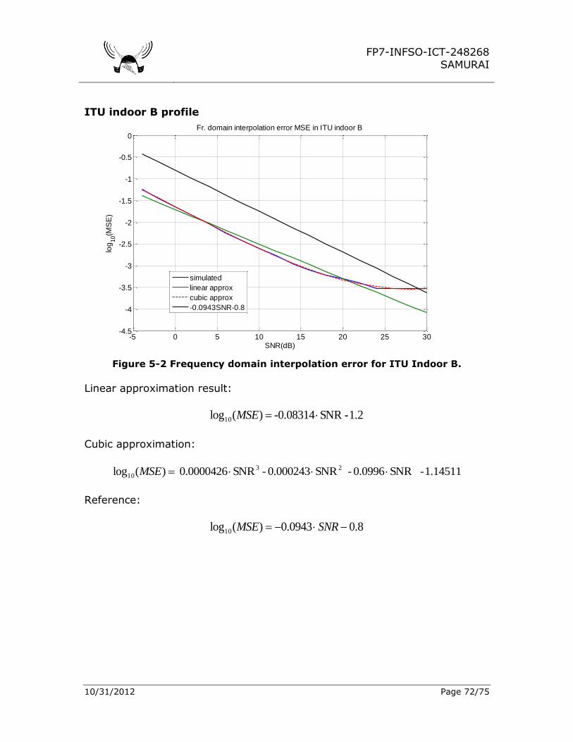
FP7-INFSO-ICT-248268
SAMURAI
10/31/2012 Page 72/75
ITU indoor B profile
Figure 5-2 Frequency domain interpolation error for ITU Indoor B.
Linear approximation result:
1.2-SNR-0.08314)(log10 MSE
Cubic approximation:
1.14511- SNR 0.0996- SNR 0.000243 -SNR0.0000426 )(log 23
10 MSE
Reference:
8.00943.0)(log10 SNRMSE
-5 0 5 10 15 20 25 30-4.5
-4
-3.5
-3
-2.5
-2
-1.5
-1
-0.5
0
SNR(dB)
log
10(M
SE
)
Fr. domain interpolation error MSE in ITU indoor B
simulated
linear approx
cubic approx
-0.0943SNR-0.8

FP7-INFSO-ICT-248268
SAMURAI
10/31/2012 Page 73/75

FP7-INFSO-ICT-248268
SAMURAI
10/31/2012 Page 74/75
ITU pedestrian B profile
Figure 5-3 Frequency domain interpolation error for ITU PedestrianB.
Linear approximation result:
16153.0 SNR0.09547- )(log10 MSE
Cubic approximation :
18401.0 SNR0.09832- SNR0.000496- SNR0.000027 )(log 23
10 MSE
Reference:
8.00943.0)(log10 SNRMSE
As Ped B is more frequency selective, interpolation error is underestimated by the reference.
-5 0 5 10 15 20 25 30-4
-3.5
-3
-2.5
-2
-1.5
-1
-0.5
0
0.5
1
SNR(dB)
log
10(M
SE
)
Fr. domain interpolation error MSE in ITU pedestrian B
simulated
linear approx
cubic approx
-0.0943SNR-0.8

FP7-INFSO-ICT-248268
SAMURAI
10/31/2012 Page 75/75
ITU vehicular B profile
Figure 5-4 Frequency domain interpolation error for ITU PedestrianB.
Linear approximation result:
05415.0 SNR0.07127- )(log10 MSE
Cubic approximation: with this very highly frequency selective channel we observe major difference in favour of the fitted cubic polynomial.
12485.0 SNR0.10115- SNR0.000656- SNR0.0000293 )(log 23
10 MSE
Reference:
8.00943.0)(log10 SNRMSE
As Veh. B is more frequency selective, interpolation error is underestimated by the reference.
-5 0 5 10 15 20 25 30-4
-3.5
-3
-2.5
-2
-1.5
-1
-0.5
0
0.5
1
SNR(dB)
log
10(M
SE
)
Fr. domain interpolation error MSE in ITU vehicular B
simulated
linear approx
cubic approx
-0.0943SNR-0.8
Related Documents