Sampling with Unequal Probabilities · Under unequal probability sampling, the variance ofY π may be considerably smaller than the variance under an equal probability sampling design

Sampling with Unequal Probabilities

1. Introduction

Since the mid 1950s, there has been a well-developed theory of sample survey designinference embracing complex designs with stratification and unequal probabilities(Smith, 2001). Unequal probability sampling was first suggested by Hansen and Hurwitz(1943) in the context of sampling with replacement. Narain (1951), Horvitz and Thomp-son (1952) developed the corresponding theory for sampling without replacement.A large part of survey sampling literature is devoted to unequal probabilities sampling,and more than 50 sampling algorithms have been proposed. Two books (Brewer andHanif, 1983; Tillé, 2006) provide a summary of these methods.

Consider a finite population U of size N. Each unit of the population can be identifiedby a label k = 1, . . . , N. A sample s is a subset of U. A sampling design p(.) is aprobability measure on all the possible samples so that

p(s) ≥ 0, for all s ∈ U, and∑

s∈U

p(s) = 1.

Let n(s) denote the size of the sample s. When the sample size is not random, we denotethe sample size by n. An unequal probability sampling design is often characterizedby its first-order inclusion probabilities given by πk = p(k ∈ s). The joint inclusionprobabilities of unit k and � are defined by πk� = p(k ∈ s and � ∈ s).

Suppose we wish to estimate the population total

Y =∑

k∈U

yk

of a characteristic of interest y, where yk is the value of a unit labeled k. An estimator ofY is given by the π-estimator (Horvitz and Thompson, 1952; Narain, 1951) defined by

Yπ =∑

k∈s

yk

πk

.

1

Published in Handbook of Statistics 29, part a, 39-54, 2009 which should be used for anyreference to this work

1

Yves G. Berger1 and Yves Tillé2

1Southampton Statistical Sciences Research Institute,University of Southampton, Southampton, UK2Institute of Statistics, University of Neuchâtel, Switzerland

This estimator is design unbiased provided that all the πk > 0.

Under unequal probability sampling, the variance of Yπ may be considerably smallerthan the variance under an equal probability sampling design (Cochran, 1963), whenthe correlation between the characteristic of interest and the first-order inclusion prob-abilities is strong. Alternative estimators when this correlation is weak are discussed inSection 3.

It is common practice to use inclusion probabilities that are proportional to a knownpositive size variable x. In this case, the inclusion probabilities are computed as follows

πk = nxk

X, (1)

where X = ∑k∈U xk, assuming nxk ≤ X for all k. If nxk > X, we set πk = 1 and we

recalculate the πk using (1) on the remaining units after substituting n with n subtractedby the number of πk equal to 1.

Another application of unequal probability sampling design is with multistage sam-pling, where the selection of primary units within strata may be done with unequalprobability. For example, self-weighted two-stage sampling is often used to select pri-mary units with probabilities that are proportional to the number of secondary unitswithin the primary units. A simple random sample is selected within each primary unit.

The variance of the π-estimator plays an important role in variance estimation, asmost estimators of interest can be linearized to involve π-estimators (see Section 5).The sampling variance of Yπ is given by

var (Yπ) =∑

k∈U

∑

�∈U

(πk� − πkπ�)yky�

πkπ�

.

Horvitz and Thompson (1952) proposed an unbiased estimator of var (Yπ):

var (Yπ) =∑

k∈s

∑

�∈s

πk� − πkπ�

πk�

yky�

πkπ�

. (2)

If the sample size is fixed, Sen (1953), Yates and Grundy (1953) proposed anotherestimator of var (Yπ):

var (Yπ) = 1

2

∑

k∈s

∑

�∈s

πkπ� − πk�

πk�

(yk

πk

− y�

π�

)2

. (3)

This estimator is design unbiased when πk� > 0 for all k, �∈ U. It can take negativevalues unless πkπ� − πk� ≥ 0, k �= � ∈ U. However, it is rarely used because the jointinclusion probabilities are sometimes difficult to compute and because the double summakes (3) computationally intensive. In Section 4, we show that, in particular cases, thevariance can be estimated without joint inclusion probabilities.

2. Some methods of unequal probability sampling

2.1. Poisson sampling

Poisson sampling was proposed by Hájek (1964) and discussed among others in Ogusand Clark (1971), Brewer et al. (1972, 1984), and Cassel et al. (1993, p. 17). Each unit

2

of the population is selected independently with a probability πk. The sample size n(s)

is therefore random. All the samples s ⊂ U have a positive probability of being selectedand there is thus a non-null probability of selecting an empty sample. The samplingdesign is given by

P(s) =[∏

k∈s

πk

1 − πk

][∏

k∈U

(1 − πk)

], for all s ⊂ U.

Since the units are selected independently, we have that πk� = πkπ�, for all k �= �.

The variance of the π-estimator, given in (2), reduces to

var(Yπ

) =∑

k∈U

1

πk

(1 − πk)y2k,

which can be unbiasedly estimated by

var(Yπ

) =∑

k∈s

(1 − πk)y2

k

π2k

.

The estimator of variance is simple because it does not involve joint inclusion probabil-ities. Note that the Poisson sampling design maximizes the entropy (Hájek, 1981, p.29)given by

I(p) = −∑

s⊂U

p(s) log p(s), (4)

subject to given inclusion probabilities πk, k ∈ U. Since the entropy is a measure ofrandomness, the Poisson sampling design can be viewed as the most random samplingdesign that satisfies given inclusion probabilities.

Poisson sampling is rarely applied in practice because its sample size is randomimplying a nonfixed cost of sampling. This design is, however, often used to modelnonresponse. Moreover, Poisson sampling will be used in Section 2.7 to define theconditional Poisson sampling design. This sampling design is also called the maximumentropy design with fixed sample size. The use of design that maximizes the entropy isuseful because it allows a simple estimation for the variance.

2.2. Sampling with replacement

Unequal probability sampling with replacement is originally due to Hanssen andHurwitz. Properties of this design are widely covered in the literature (Bol’shev, 1965;Brown and Bromberg, 1984; Dagpunar, 1988; Davis, 1993; Devroye, 1986; Ho et al.,1979; Johnson et al., 1997; Kemp and Kemp, 1987; Loukas and Kemp, 1983; Tillé,2006).

Consider selection probabilities pk that are proportional to a positive size variablexk, k ∈ U; that is,

pk = xk∑�∈U x�

, k ∈ U.

A simple method to select a sample with unequal probabilities with replacement con-sists in generating a uniform random number u in [0, 1] and selecting unit k so that AQ:1

3

vk−1 ≤ u < vk, where

vk =k∑

�=1

p�, with v0 = 0.

This process is repeated independently m times. Note that there are more efficient algo-rithms that may be used to select a sample with replacement with unequal probabilities(Tillé, 2006, p. 75).

Let yi denote the value of the characteristic of the ith selected unit and pi, its associatedselection probability. Note that, under sampling with replacement, the same unit can beselected several times. The ratios yi/pi are n independent random variables. The totalY can be estimated by the Hansen–Hurwitz estimator

YHH = 1

m

m∑

i=1

yi

pi

.

This estimator is design unbiased as

E(YHH

) = 1

m

m∑

i=1

E

(yi

pi

)= 1

m

m∑

i=1

Y = Y.

The variance of YHH is given by

var (YHH) = 1

m

∑

k∈U

pk

(yk

pk

− Y

)2

,

which can be unbiasedly estimated by

var (YHH) = 1

m(m − 1)

m∑

i=1

(yi

pi

− YHH

)2

. (5)

The Hansen–Hurwitz estimator is not the best estimator as it is not admissible becauseit depends on the multiplicity of the units (Basu, 1958, 1969; Basu and Ghosh, 1967).Nevertheless, the Hansen–Hurwitz variance estimator can be used to approximate thevariance of the Horvitz–Thompson estimator under sampling without replacement whenm/N is small.

Sampling without replacement may lead to a reduction of the variance compared tosampling with replacement (Gabler, 1981, 1984). A design without replacement withinclusion probabilities πk is considered to be a good design if the Horvitz–Thompsonestimator is always more accurate than the Hansen–Hurwitz estimator under samplingwith replacement with probabilities pk = πk/n. Gabler (1981, 1984) gave a condi-tion under which this condition holds. For example, this condition holds for the Rao–Sampford design given in Section 2.4 and for the maximum entropy design with fixedsample size (Qualité, 2008).

2.3. Systematic sampling

Systematic sampling is widely used by statistical offices due to its simplicity and effi-ciency (Bellhouse, 1988; Bellhouse and Rao, 1975; Berger, 2003; Iachan, 1982, 1983).

4

This sampling design has been studied since the early years of survey sampling (Cochran,1946; Madow, 1949; Madow and Madow, 1944). There are two types of systematic sam-pling: a systematic sample can be selected from a deliberately ordered population or thepopulation can be randomized before selecting a systematic sample. The latter is oftencalled randomized systematic design.

In many practical situations, it is common practice to let the population frame have apredetermined order. For example, a population frame can be sorted by a size variable,by region, by socioeconomic group, by postal sector, or in some other way. In this case,systematic sampling is an efficient method of sampling (Iachan, 1982). Systematic sam-pling from a deliberately ordered population is generally more accurate than randomizedsystematic sampling (Särndal et al., 1992, p. 81), especially when there is a trend in thesurvey variable y (Bellhouse and Rao, 1975).

A systematic sample is selected as follows. Let u be a random number between 0 and1 generated from a uniform distribution. A systematic sample is a set of n units labeledk1, k2, . . . , kn such that π

(c)

k�−1 < u + � − 1 ≤ π(c)

k�, where � = 1, . . . , n and

π(c)

k =∑

j∈Uj≤k

πj.

In the special case where πk = n/N, this design reduces to the customary systematicsampling design, where every ath unit is selected and a = �N/n�.

The systematic design with a deliberately ordered population suffers from a seri-ous flaw, namely, that it is impossible to unbiasedly estimate the sampling variance(Iachan, 1982), and customary variance estimators given in (3) are inadequate and canoverestimate the variance significantly (Särndal et al., 1992, Chapter 3).

Systematic sampling from a randomly ordered population consists in randomlyarranging the units, giving the same probability to each permutation, since randomordering is part of the sampling design. This design was first suggested by Madow(1949). Hartley and Rao (1962) developed the corresponding asymptotic theory forlarge N and small sampling fraction. Under randomized systematic sampling, Hartleyand Rao (1962) derived a design unbiased variance estimator (see Section 4).

For the randomized systematic design, the joint inclusion probabilities are typicallypositive and the variance can be unbiasedly estimated (Hájek, 1981; Hartley and Rao,1962). With a deliberately ordered population, alternative estimators for the variancecan be used (Bartolucci and Montanari, 2006; Berger, 2005a; Brewer, 2002, Chapter 9).

2.4. Rao–Sampford sampling design

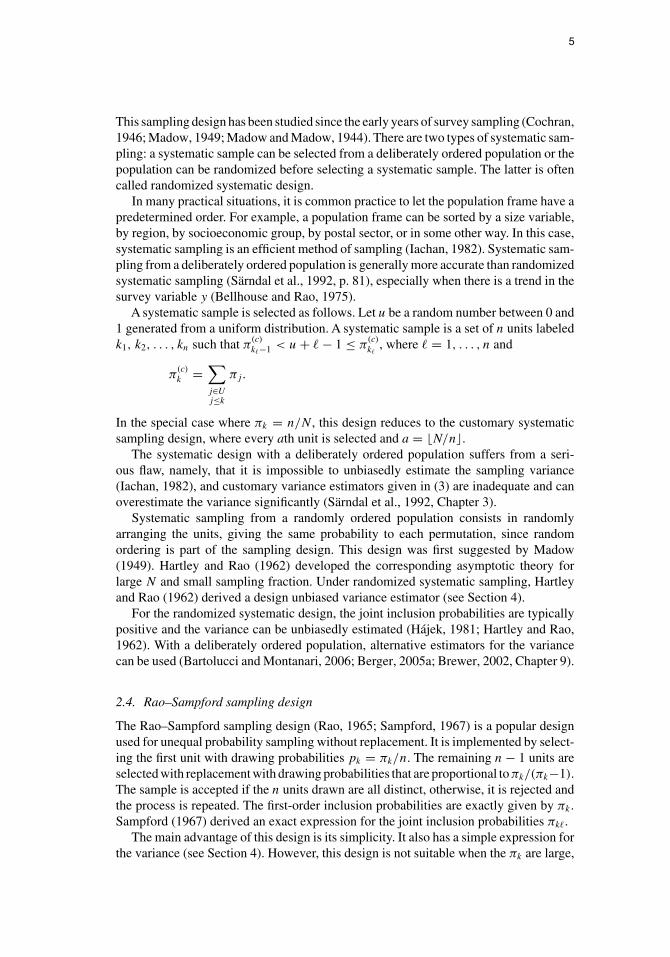
The Rao–Sampford sampling design (Rao, 1965; Sampford, 1967) is a popular designused for unequal probability sampling without replacement. It is implemented by select-ing the first unit with drawing probabilities pk = πk/n. The remaining n − 1 units areselected with replacement with drawing probabilities that are proportional toπk/(πk−1).The sample is accepted if the n units drawn are all distinct, otherwise, it is rejected andthe process is repeated. The first-order inclusion probabilities are exactly given by πk.

Sampford (1967) derived an exact expression for the joint inclusion probabilities πk�.The main advantage of this design is its simplicity. It also has a simple expression for

the variance (see Section 4). However, this design is not suitable when the πk are large,

5

as we would almost surely draw the units with large πk at least twice and it would not bepossible to select one Rao–Sampford sample. For example, consider N = 86, n = 36,and πk proportional to (k/100)5 + 1/5. The probability that all the units drawn fromsubsequent independent draws will be distinct is approximately 10−36 (Hájek, 1981,p. 70), which is negligible. Nevertheless, Tillé (2006, p. 136) and Bondesson et al. (2006)suggested several alternative algorithms to implement the Rao–Sampford design.

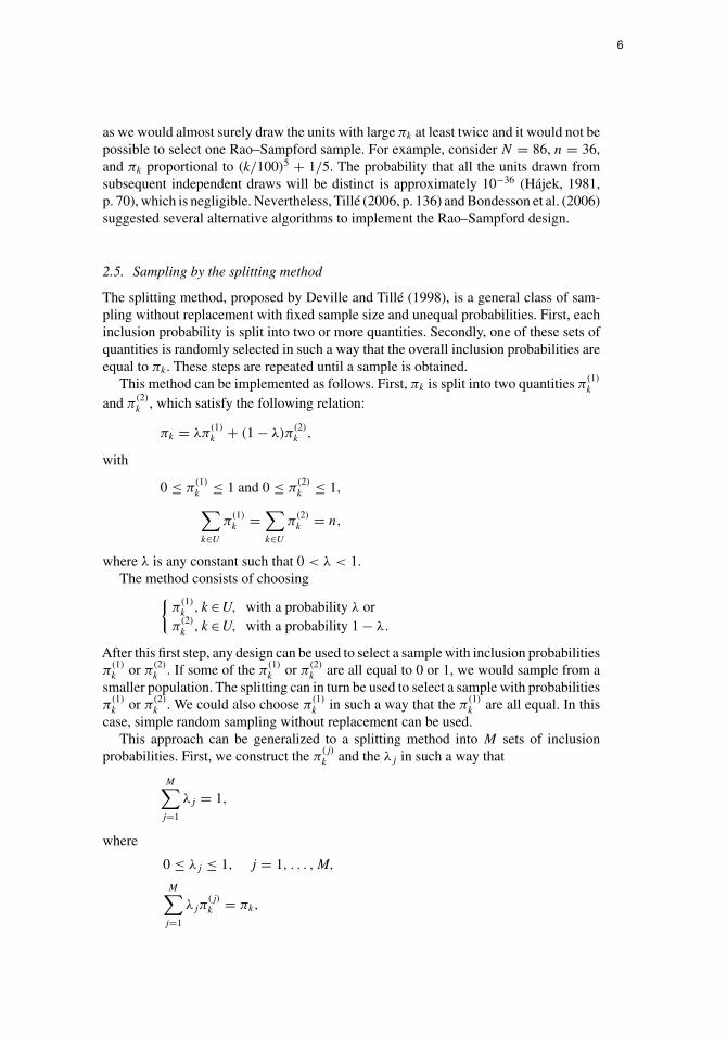
2.5. Sampling by the splitting method

The splitting method, proposed by Deville and Tillé (1998), is a general class of sam-pling without replacement with fixed sample size and unequal probabilities. First, eachinclusion probability is split into two or more quantities. Secondly, one of these sets ofquantities is randomly selected in such a way that the overall inclusion probabilities areequal to πk. These steps are repeated until a sample is obtained.

This method can be implemented as follows. First, πk is split into two quantities π(1)

k

and π(2)

k , which satisfy the following relation:

πk = λπ(1)

k + (1 − λ)π(2)

k ,

with

0 ≤ π(1)

k ≤ 1 and 0 ≤ π(2)

k ≤ 1,

∑

k∈U

π(1)

k =∑

k∈U

π(2)

k = n,

where λ is any constant such that 0 < λ < 1.

The method consists of choosing{

π(1)

k , k ∈ U, with a probability λ orπ

(2)

k , k ∈ U, with a probability 1 − λ.

After this first step, any design can be used to select a sample with inclusion probabilitiesπ

(1)

k or π(2)

k . If some of the π(1)

k or π(2)

k are all equal to 0 or 1, we would sample from asmaller population. The splitting can in turn be used to select a sample with probabilitiesπ

(1)

k or π(2)

k . We could also choose π(1)

k in such a way that the π(1)

k are all equal. In thiscase, simple random sampling without replacement can be used.

This approach can be generalized to a splitting method into M sets of inclusionprobabilities. First, we construct the π

(j)

k and the λj in such a way that

M∑

j=1

λj = 1,

where

0 ≤ λj ≤ 1, j = 1, . . . , M,

M∑

j=1

λjπ(j)

k = πk,

6

0 ≤ π(j)

k ≤ 1, k ∈ U, j = 1, . . . , M,∑

k∈U

π(j)

k = n, j = 1, . . . , M.

We then select one of the set of quantities of π(j)

k , k ∈ U, with probabilities λj , j =1, . . . , M. After this first step, any design can be used to select a sample with inclusionprobabilities π

(j)

k or the splitting step can be applied again.Deville and Tillé (1998) showed that the splitting method defines new sampling

designs such as the minimum support design, the splitting into simple random sampling,the pivotal method, and the eliminatory method (Tillé, 2006).

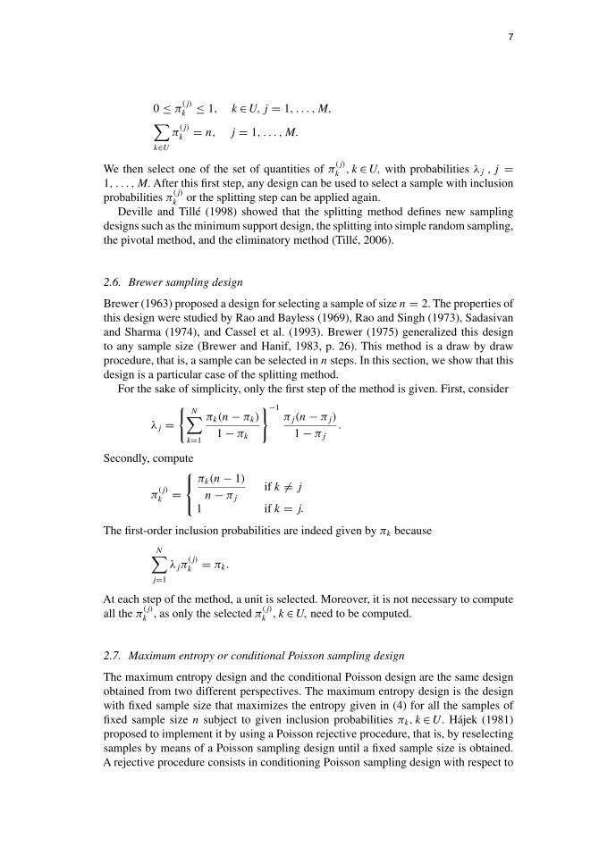
2.6. Brewer sampling design

Brewer (1963) proposed a design for selecting a sample of size n = 2. The properties ofthis design were studied by Rao and Bayless (1969), Rao and Singh (1973), Sadasivanand Sharma (1974), and Cassel et al. (1993). Brewer (1975) generalized this designto any sample size (Brewer and Hanif, 1983, p. 26). This method is a draw by drawprocedure, that is, a sample can be selected in n steps. In this section, we show that thisdesign is a particular case of the splitting method.

For the sake of simplicity, only the first step of the method is given. First, consider

λj ={

N∑

k=1

πk(n − πk)

1 − πk

}−1πj(n − πj)

1 − πj

.

Secondly, compute

π(j)

k =⎧⎨

⎩

πk(n − 1)

n − πj

if k �= j

1 if k = j.

The first-order inclusion probabilities are indeed given by πk because

N∑

j=1

λjπ(j)

k = πk.

At each step of the method, a unit is selected. Moreover, it is not necessary to computeall the π

(j)

k , as only the selected π(j)

k , k ∈ U, need to be computed.

2.7. Maximum entropy or conditional Poisson sampling design

The maximum entropy design and the conditional Poisson design are the same designobtained from two different perspectives. The maximum entropy design is the designwith fixed sample size that maximizes the entropy given in (4) for all the samples offixed sample size n subject to given inclusion probabilities πk, k ∈ U. Hájek (1981)proposed to implement it by using a Poisson rejective procedure, that is, by reselectingsamples by means of a Poisson sampling design until a fixed sample size is obtained.A rejective procedure consists in conditioning Poisson sampling design with respect to

7

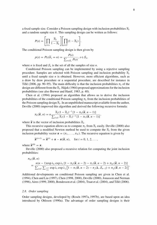
a fixed sample size. Consider a Poisson sampling design with inclusion probabilities πk

and a random sample size n. This sampling design can be written as follows:

P(s) =[∏

k∈s

πk

1 − πk

][∏

k∈U

(1 − πk)

].

The conditional Poisson sampling design is then given by

p(s) = P(s|ns = n) = P(s)∑s∈Sn

P(s), s ∈ Sn,

where n is fixed and Sn is the set of all the samples of size n.Conditional Poisson sampling can be implemented by using a rejective sampling

procedure. Samples are selected with Poisson sampling and inclusion probability πk

until a fixed sample size n is obtained. However, more efficient algorithms, such asa draw by draw procedure or a sequential procedure, are described for instance inTillé (2006, pp. 90–95). The main difficulty is that the inclusion probabilities πk of thedesign are different from the πk. Hájek (1964) proposed approximations for the inclusionprobabilities (see also Brewer and Hanif, 1983, p. 40).

Chen et al. (1994) proposed an algorithm that allows us to derive the inclusionprobabilities of the conditional Poisson sampling πk from the inclusion probabilities ofthe Poisson sampling design πk. In an unpublished manuscript available from the author,Deville (2000) improved this algorithm and derived the following recursive formula:

πk(π, n) = nπk(1 − πk)

−1 [1 − πk(π, n − 1)]∑�∈U π�(1 − π�)−1 [1 − π�(π, n − 1)]

,

where π is the vector of inclusion probabilities πk.

This recursive equation allows us to compute πk from πk easily. Deville (2000) alsoproposed that a modified Newton method be used to compute the πk from the giveninclusion probability vector π = (π1, . . . , πN). The recursive equation is given by

π(i+1) = π(i) + π − π(π, n), for i = 0, 1, 2, . . . ,

where π(0) = π.Deville (2000) also proposed a recursive relation for computing the joint inclusion

probabilities:

πk�(π, n)

= n(n − 1)exp λk exp λ� [1 − πk(π, n − 2) − π�(π, n − 2) + πk�(π, n − 2)]∑

i∈U

∑j∈U

i�=jexp λi exp λj

[1 − πi(π, n − 2) − πj(λ, Sn−2) + πij(π, n − 2)

] ,

Additional developments on conditional Poisson sampling are given in Chen et al.(1994), Chen and Liu (1997), Chen (1998, 2000), Deville (2000), Jonasson and Nerman(1996), Aires (1999, 2000), Bondesson et al. (2004), Traat et al. (2004), and Tillé (2006).

2.8. Order sampling

Order sampling designs, developed by (Rosén 1997a, 1997b), are based upon an ideaintroduced by Ohlsson (1990a). The advantage of order sampling designs is their

8

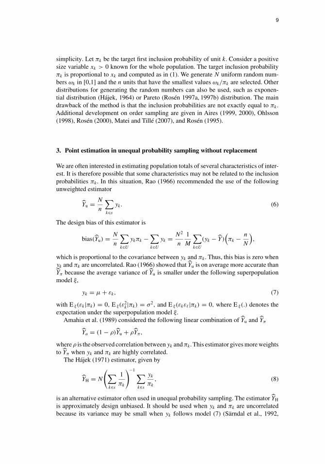
simplicity. Let πk be the target first inclusion probability of unit k. Consider a positivesize variable xk > 0 known for the whole population. The target inclusion probabilityπk is proportional to xk and computed as in (1). We generate N uniform random num-bers ωk in [0,1] and the n units that have the smallest values ωk/πk are selected. Otherdistributions for generating the random numbers can also be used, such as exponen-tial distribution (Hájek, 1964) or Pareto (Rosén 1997a, 1997b) distribution. The maindrawback of the method is that the inclusion probabilities are not exactly equal to πk.

Additional development on order sampling are given in Aires (1999, 2000), Ohlsson(1998), Rosén (2000), Matei and Tillé (2007), and Rosén (1995).

3. Point estimation in unequal probability sampling without replacement

We are often interested in estimating population totals of several characteristics of inter-est. It is therefore possible that some characteristics may not be related to the inclusionprobabilities πk. In this situation, Rao (1966) recommended the use of the followingunweighted estimator

Yu = N

n

∑

k∈s

yk. (6)

The design bias of this estimator is

bias(Yu) = N

n

∑

k∈U

ykπk −∑

k∈U

yk = N2

n

1

M

∑

k∈U

(yk − Y )(πk − n

N

),

which is proportional to the covariance between yk and πk. Thus, this bias is zero whenyk and πk are uncorrelated. Rao (1966) showed that Yu is on average more accurate thanYπ because the average variance of Yu is smaller under the following superpopulationmodel ξ,

yk = μ + εk, (7)

with E ξ(εk|πk) = 0, E ξ(ε2k|πk) = σ2, and E ξ(εkε�|πk) = 0, where E ξ(.) denotes the

expectation under the superpopulation model ξ.Amahia et al. (1989) considered the following linear combination of Yu and Yπ

Ya = (1 − ρ)Yu + ρYπ,

where ρ is the observed correlation between yk and πk. This estimator gives more weightsto Yπ when yk and πk are highly correlated.

The Hájek (1971) estimator, given by

YH = N

(∑

k∈s

1

πk

)−1∑

k∈s

yk

πk

, (8)

is an alternative estimator often used in unequal probability sampling. The estimator YH

is approximately design unbiased. It should be used when yk and πk are uncorrelatedbecause its variance may be small when yk follows model (7) (Särndal et al., 1992,

9

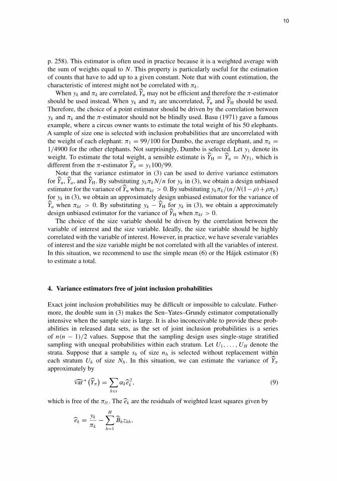
p. 258). This estimator is often used in practice because it is a weighted average withthe sum of weights equal to N. This property is particularly useful for the estimationof counts that have to add up to a given constant. Note that with count estimation, thecharacteristic of interest might not be correlated with πk.

When yk and πk are correlated, Yu may not be efficient and therefore the π-estimatorshould be used instead. When yk and πk are uncorrelated, Yu and YH should be used.Therefore, the choice of a point estimator should be driven by the correlation betweenyk and πk and the π-estimator should not be blindly used. Basu (1971) gave a famousexample, where a circus owner wants to estimate the total weight of his 50 elephants.A sample of size one is selected with inclusion probabilities that are uncorrelated withthe weight of each elephant: π1 = 99/100 for Dumbo, the average elephant, and πk =1/4900 for the other elephants. Not surprisingly, Dumbo is selected. Let y1 denote itsweight. To estimate the total weight, a sensible estimate is YH = Yu = Ny1, which isdifferent from the π-estimator Yπ = y1100/99.

Note that the variance estimator in (3) can be used to derive variance estimatorsfor Yu, Ya, and YH. By substituting ykπkN/n for yk in (3), we obtain a design unbiasedestimator for the variance of Yu when πk� > 0. By substituting ykπk/(n/N(1−ρ)+ρπk)

for yk in (3), we obtain an approximately design unbiased estimator for the variance ofYa when πk� > 0. By substituting yk − YH for yk in (3), we obtain a approximatelydesign unbiased estimator for the variance of YH when πk� > 0.

The choice of the size variable should be driven by the correlation between thevariable of interest and the size variable. Ideally, the size variable should be highlycorrelated with the variable of interest. However, in practice, we have severale variablesof interest and the size variable might be not correlated with all the variables of interest.In this situation, we recommend to use the simple mean (6) or the Hájek estimator (8)to estimate a total.

4. Variance estimators free of joint inclusion probabilities

Exact joint inclusion probabilities may be difficult or impossible to calculate. Futher-more, the double sum in (3) makes the Sen–Yates–Grundy estimator computationallyintensive when the sample size is large. It is also inconceivable to provide these prob-abilities in released data sets, as the set of joint inclusion probabilities is a seriesof n(n − 1)/2 values. Suppose that the sampling design uses single-stage stratifiedsampling with unequal probabilities within each stratum. Let U1, . . . , UH denote thestrata. Suppose that a sample sh of size nh is selected without replacement withineach stratum Uh of size Nh. In this situation, we can estimate the variance of Yπ

approximately by

var ∗ (Yπ

) =∑

k∈s

αke2k , (9)

which is free of the πl�. The ek are the residuals of weighted least squares given by

ek = yk

πk

−H∑

h=1

Bhzkh,

10

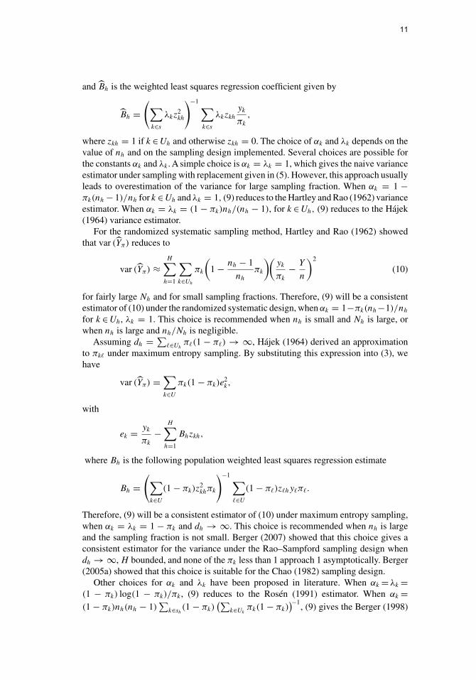
and Bh is the weighted least squares regression coefficient given by

Bh =(∑

k∈s

λkz2kh

)−1∑

k∈s

λkzkh

yk

πk

,

where zkh = 1 if k ∈ Uh and otherwise zkh = 0. The choice of αk and λk depends on thevalue of nh and on the sampling design implemented. Several choices are possible forthe constants αk and λk. A simple choice is αk = λk = 1, which gives the naive varianceestimator under sampling with replacement given in (5). However, this approach usuallyleads to overestimation of the variance for large sampling fraction. When αk = 1 −πk(nh − 1)/nh for k ∈ Uh and λk = 1, (9) reduces to the Hartley and Rao (1962) varianceestimator. When αk = λk = (1 − πk)nh/(nh − 1), for k ∈ Uh, (9) reduces to the Hájek(1964) variance estimator.

For the randomized systematic sampling method, Hartley and Rao (1962) showedthat var (Yπ) reduces to

var (Yπ) ≈H∑

h=1

∑

k∈Uh

πk

(1 − nh − 1

nh

πk

)(yk

πk

− Y

n

)2

(10)

for fairly large Nh and for small sampling fractions. Therefore, (9) will be a consistentestimator of (10) under the randomized systematic design, when αk = 1−πk(nh−1)/nh

for k ∈ Uh, λk = 1. This choice is recommended when nh is small and Nh is large, orwhen nh is large and nh/Nh is negligible.

Assuming dh = ∑�∈Uh

π�(1 − π�) → ∞, Hájek (1964) derived an approximationto πk� under maximum entropy sampling. By substituting this expression into (3), wehave

var (Yπ) =∑

k∈U

πk(1 − πk)e2k,

with

ek = yk

πk

−H∑

h=1

Bhzkh,

where Bh is the following population weighted least squares regression estimate

Bh =(∑

k∈U

(1 − πk)z2khπk

)−1∑

�∈U

(1 − π�)z�hy�π�.

Therefore, (9) will be a consistent estimator of (10) under maximum entropy sampling,when αk = λk = 1 − πk and dh → ∞. This choice is recommended when nh is largeand the sampling fraction is not small. Berger (2007) showed that this choice gives aconsistent estimator for the variance under the Rao–Sampford sampling design whendh → ∞, H bounded, and none of the πk less than 1 approach 1 asymptotically. Berger(2005a) showed that this choice is suitable for the Chao (1982) sampling design.

Other choices for αk and λk have been proposed in literature. When αk = λk =(1 − πk) log(1 − πk)/πk, (9) reduces to the Rosén (1991) estimator. When αk =(1 − πk)nh(nh − 1)

∑k∈sh

(1 − πk)(∑

k∈Ukπk(1 − πk)

)−1, (9) gives the Berger (1998)

11

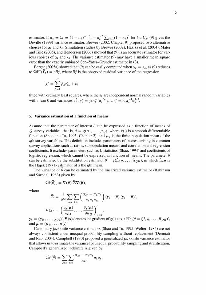
estimator. If αk = λk = (1 − πk)−1[1 − d−2

h

∑�∈sh

(1 − π�)]

for k ∈ Uh, (9) gives theDeville (1999) variance estimator. Brewer (2002, Chapter 9) proposed two alternativechoices for αk and λk. Simulation studies by Brewer (2002), Haziza et al. (2004), Mateiand Tillé (2005), and Henderson (2006) showed that (9) is an accurate estimator for var-ious choices of αk and λk. The variance estimator (9) may have a smaller mean squareerror than the exactly unbiased Sen–Yates–Grundy estimator in (3).

Berger (2005a) showed that (9) can be easily computed when αk = λk, as (9) reducesto var ∗(Yπ) = nσ2

ε , where σ2ε is the observed residual variance of the regression

y∗k =

H∑

h=1

βhz∗�h + εk

fitted with ordinary least squares, where the εk are independent normal random variableswith mean 0 and variances σ2

ε , y∗k = ykπ

−1k α

1/2k and z∗

k = zkπ−1k α

1/2k .

5. Variance estimation of a function of means

Assume that the parameter of interest θ can be expressed as a function of means ofQ survey variables, that is, θ = g(μ1, . . . , μQ), where g(.) is a smooth differentiablefunction (Shao and Tu, 1995, Chapter 2), and μq is the finite population mean of theqth survey variables. This definition includes parameters of interest arising in commonsurvey applications such as ratios, subpopulation means, and correlation and regressioncoefficients. It excludes parameters such as L-statistics (Shao, 1994) and coefficients oflogistic regression, which cannot be expressed as function of means. The parameter θ

can be estimated by the substitution estimator θ = g(μ1H, . . . , μQH), in which μqH isthe Hájek (1971) estimator of a the qth mean.

The variance of θ can be estimated by the linearized variance estimator (Rabinsonand Särndal, 1983) given by

var(θ)l = ∇(μ)′ ∇(μ),

where

= 1

N2

∑

k∈s

∑

�∈s

(πk� − πkπ�

πkπ�πk�

)(yk − μ) (y� − μ)′,

∇(x) =(

∂g(μ)

∂μ1, . . . ,

∂g(μ)

∂μQ

)′

μ=x

,

yk = (y1k, . . . , yQk)′, ∇(x) denotes the gradient of g(·) at x ∈R

Q, μ = (μ1H, . . . , μQH)′,and μ = (μ1, . . . , μQ)′.

Customary jackknife variance estimators (Shao and Tu, 1995; Wolter, 1985) are notalways consistent under unequal probability sampling without replacement (Demnatiand Rao, 2004). Campbell (1980) proposed a generalized jackknife variance estimatorthat allows us to estimate the variance for unequal probability sampling and stratification.Campbell’s generalized jackknife is given by

var (θ) =∑

k∈s

∑

�∈s

πk� − πkπ�

πk�

uku�,

12

where

uj = (1 − wj)(θ − θ(j)),

wj = π−1j

(∑

k∈s

π−1k

)−1

,

θ(j) = g(μ1H(j), . . . , μQH(j)),

μqH(j) = N

(∑

k∈s

δkj

πk

)−1∑

k∈s

δkjyk

πk

,

and δkj = 1 if k = j and δkj = 0 otherwise. Berger and Skinner (2005) gave regularityconditions under which the generalized jackknife is consistent. They also showed thatthe generalized jackknife may be more accurate than the customary jackknife estimators.Berger (2007) proposed an alternative consistent jackknife estimator that is free of jointinclusion probabilities.

Many surveys use single imputation to handle item nonresponse. Treating the imputedvalues as if they were true values and then estimating the variance using standardmethods may lead to serious underestimation of the variance when the proportion ofmissing values is large (Rao and Shao, 1992; Särndal, 1992). One can use the Rao–Shaomethod which consists of adjusting the imputed values whenever a responding unit isdeleted. Berger and Rao (2006) showed that this method gives a consistent generalizedjackknife variance estimator under uniform response.

6. Balanced sampling

6.1. Definition

A design is balanced if the π-estimators for a set of auxiliary variables are equal to theknown population totals of auxiliary variables. Balanced sampling can be viewed asa calibration method embedded into the sampling design. Yates (1949) advocated theidea of respecting the means of known variables in probability samples. Yates (1946)and Neyman (1934) described methods of balanced sampling limited to one variableand to equal inclusion probabilities. The use of balanced sampling was recommend byRoyall and Herson (1973) for protecting inference against misspecified models. Morerecently, several partial solutions were proposed by Deville et al. (1988), Deville (1992),Ardilly (1991), and Hedayat and Majumdar (1995). Valliant et al. (2000) surveyed someexisting methods.

The cube method (Deville and Tillé, 2004) is a general method of balanced samplingwith equal or unequal inclusion probabilities. Properties and application of this methodwere studied in Deville and Tillé (2004), Chauvet and Tillé (2006), Tillé and Favre(2004, 2005), Berger et al. (2003), and Nedyalkova and Tillé (2008). The cube methodwas used to select the rotation groups of the new French census (Bertrand et al., 2004;Dumais and Isnard, 2000; Durr and Dumais, 2002) and the selection of the Frenchmaster sample (Christine, 2006; Christine and Wilms, 2003; Wilms, 2000). Deville andTillé (2005) proposed a variance estimator for balanced sampling. Deville (2006) alsoproposed to use balanced sampling for the imputation of item nonresponse. The cube

13

method can be implemented in practice by SAS or R procedures (Chauvet and Tillé,AQ:22005; Rousseau and Tardieu, 2004; Tardieu, 2001; Tillé and Matei, 2007).

Balancing is used when auxiliary information is available at the design stage. Whenbalanced sampling is used, the Horvitz–Thompson weights are also calibration weights.Calibration after sampling is therefore not necessary. Balancing also provide more stableestimators as these weights do not depend on the sample.

6.2. Balanced sampling and the cube method

Suppose that the values of p auxiliary variables x1, . . . xp are known for every unit ofthe population. Let xk = (xk1 · · · xkj · · · xkp)′ be the vector of the p auxiliary variables onunit k. For a set of given inclusion probabilities πk, a design p(.) is said to be balancedwith respect to the auxiliary variables x1, . . . , xp, if and only if it satisfies the balancingequations given by

∑

k∈s

xk

πk

=∑

k∈U

xk. (11)

Balanced sampling generalizes several well-known methods. For instance, if xk = πk,

then (11) is a fixed size constraint. It can be shown that, if the auxiliary variables are theindicator variables of strata, a stratified sampling design is balanced on these indicatorvariables.

However, it is often not possible to find a sample such that (11) holds, for exam-ple, when the right-hand side of (11) is an integer. Hence, an exactly balanced designoften does not exist. For example, if x1 = 1, x2 = 1, x3 = 1, x1 = 5, and πk = 1/2, fori = 1, 2, 3, 4, the balancing equation becomes

∑

k∈s

2xk =∑

k∈U

xk = 11, (12)

which cannot hold. The aim is thus to select an exact balanced sample if possible, andan approximately balanced sample otherwise.

The name “cube method” comes from the geometrical representation of a samplingdesign. A sample can be written as a vector s = (s1, . . . , sN) ∈ R

N of indicator variablessk that take the value 1 if the unit is selected and 0 otherwise. Geometrically, each vectors can be viewed as one of the 2N vertices of a N-cube in R

N . A design consists thusin allocating a probability p(.) to each vertex of the N cube in such a way that theexpectation of s is equal to the inclusion probability vector π, that is,

E(s) =∑

s∈Sp(s)s = π,

where π ∈ RN is the vector of inclusion probabilities. Thus, selecting a sample consists

in choosing a vertex (a sample) of the N-cube that is balanced.The balancing equations in (11) can also be written as

∑

k∈U

aksk =∑

k∈U

akπk with sk ∈ {0, 1}, k ∈ U,

14

where ak = xk/πk, k ∈ U. The balancing equations define an affine subspace in RN

of dimension N − p denoted Q. The subspace Q can be written as π + KerA, whereKerA = {u ∈ R|Au} and A = (a1 · · · an · · · aN).

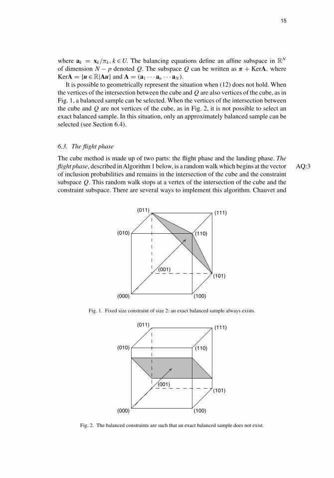
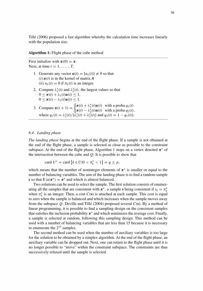
It is possible to geometrically represent the situation when (12) does not hold. Whenthe vertices of the intersection between the cube and Q are also vertices of the cube, as inFig. 1, a balanced sample can be selected. When the vertices of the intersection betweenthe cube and Q are not vertices of the cube, as in Fig. 2, it is not possible to select anexact balanced sample. In this situation, only an approximately balanced sample can beselected (see Section 6.4).

6.3. The flight phase

The cube method is made up of two parts: the flight phase and the landing phase. Theflight phase, described inAlgorithm 1 below, is a random walk which begins at the vector AQ:3of inclusion probabilities and remains in the intersection of the cube and the constraintsubspace Q. This random walk stops at a vertex of the intersection of the cube and theconstraint subspace. There are several ways to implement this algorithm. Chauvet and

(000) (100)

(101)(001)

(010) (110)

(111)(011)

Fig. 1. Fixed size constraint of size 2: an exact balanced sample always exists.

(000) (100)

(101)(001)

(010) (110)

(111)(011)

Fig. 2. The balanced constraints are such that an exact balanced sample does not exist.

15

Tillé (2006) proposed a fast algorithm whereby the calculation time increases linearlywith the population size.

Algorithm 1: Flight phase of the cube method

First initialize with π(0) = π.

Next, at time t = 1, . . . . , T,

1. Generate any vector u(t) = [uk(t)] �= 0 so that(i) u(t) is in the kernel of matrix A(ii) uk(t) = 0 if πk(t) is an integer.

2. Compute λ∗1(t) and λ∗

2(t), the largest values so that0 ≤ π(t) + λ1(t)u(t) ≤ 1,

0 ≤ π(t) − λ2(t)u(t) ≤ 1.

3. Compute π(t + 1) ={π(t) + λ∗

1(t)u(t) with a proba q1(t)

π(t) − λ∗2(t)u(t) with a proba q2(t),

where q1(t) = λ∗2(t)/{λ∗

1(t) + λ∗2(t)} and q2(t) = 1 − q1(t)}.

6.4. Landing phase

The landing phase begins at the end of the flight phase. If a sample is not obtained atthe end of the flight phase, a sample is selected as close as possible to the constraintsubspace. At the end of the flight phase, Algorithm 1 stops on a vertex denoted π∗ ofthe intersection between the cube and Q. It is possible to show that

card U∗ = card{k ∈ U|0 < π∗

k < 1} = q ≤ p,

which means that the number of noninteger elements of π∗ is smaller or equal to thenumber of balancing variables. The aim of the landing phase is to find a random samples so that E (s|π∗) = π∗ and which is almost balanced.

Two solutions can be used to select the sample. The first solution consists of enumer-ating all the samples that are consistent with π∗, a sample s being consistent if sk = π∗

k

when π∗k is an integer. Then, a cost C(s) is attached at each sample. This cost is equal

to zero when the sample is balanced and which increases when the sample moves awayfrom the subspace Q. Deville and Tillé (2004) proposed several C(s). By a method oflinear programming, it is possible to find a sampling design on the consistent samplesthat satisfies the inclusion probability π∗ and which minimizes the average cost. Finally,a sample is selected at random, following this sampling design. This method can beused with a number of balancing variables that are less than 15 because it is necessaryto enumerate the 215 samples.

The second method can be used when the number of auxiliary variables is too largefor the solution to be obtained by a simplex algorithm. At the end of the flight phase, anauxiliary variable can be dropped out. Next, one can return to the flight phase until it isno longer possible to “move” within the constraint subspace. The constraints are thussuccessively relaxed until the sample is selected.

16

Author QueriesAQ:1 Please confirm whether the closing parenthesis in [1,0) in the sentence “A sim-ple method to seleet a sample...” changed to square bracket is ok.‘AQ:2 Please define “SAS” in the sentence “Deville (2006) also proposed to use bal-anced...”AQ:3 Please confirm “Algorithm 2 changed to Algorithm 1” is ok.

17