Sampling Weights, Model Misspecification and Informative Sampling: A Simulation Study Marianne (Marnie) Bertolet * Department of Statistics Carnegie Mellon University Abstract Linear mixed-effects (LME) models analyze data that contain complex patterns of vari- ability, specifically involving different nested layers. While LME models can match well the stratification and clustering of survey data, it is not clear how sampling weights should be incorporated into LME estimates. This report uses twelve simulation studies to compare two published methods of inserting sampling weights into LME estimates, Pfeffermann et al. (1998), denoted PSHGR, and Rabe-Hesketh and Skrondal (2006), denoted RHS. There are five main conclusions based on these simulations. 1) The PSHGR and RHS point estimates are very similar, with differences due to numerical instabilities in the es- timation procedures. 2) Confidence intervals based on the sandwich estimator and the design based estimator of the variances provide similar coverage when there is no model misspecification. However, when there is model misspecification, the design-based variance estimator has unexpectedly large coverage, implying that the variance estimates are too large. 3) When there is model misspecification that does not induce informative sampling, weighted estimates do not reduce bias of the estimators. 4) When there is informative sam- pling, the weighted estimators do reduce the bias of the point estimates, though they do not eliminate it. 5) The unweighted estimate has the smallest variance. When there is in- formative sampling, the unweighted estimates are biased. The weighted unscaled estimate corrects the bias in the fixed effects, but produces more bias in the random effects. The scaled 1 weightings remove the bias in the fixed effects, and overcorrect for the weighted unscaled bias in the random effects. The scaled 2 weightings remove the bias in the fixed effects and are in between the weighted unscaled and weighted scaled 1 bias in the random effects. Keywords: Linear mixed-effects models, survey sampling, weighting bias, sampling bias, sandwich estimator, design-based estimators. * This work is based on my thesis, completed at Carneige Mellon University. Current affiliation is with the Epidemiology Data Center, Department of Epidemiology, Graduate School of Public Health, University of Pittsburgh, [email protected] 1

Welcome message from author
This document is posted to help you gain knowledge. Please leave a comment to let me know what you think about it! Share it to your friends and learn new things together.
Transcript

Sampling Weights, Model Misspecification and Informative
Sampling: A Simulation Study
Marianne (Marnie) Bertolet∗
Department of StatisticsCarnegie Mellon University
AbstractLinear mixed-effects (LME) models analyze data that contain complex patterns of vari-
ability, specifically involving different nested layers. While LME models can match well thestratification and clustering of survey data, it is not clear how sampling weights should beincorporated into LME estimates. This report uses twelve simulation studies to comparetwo published methods of inserting sampling weights into LME estimates, Pfeffermannet al. (1998), denoted PSHGR, and Rabe-Hesketh and Skrondal (2006), denoted RHS.There are five main conclusions based on these simulations. 1) The PSHGR and RHSpoint estimates are very similar, with differences due to numerical instabilities in the es-timation procedures. 2) Confidence intervals based on the sandwich estimator and thedesign based estimator of the variances provide similar coverage when there is no modelmisspecification. However, when there is model misspecification, the design-based varianceestimator has unexpectedly large coverage, implying that the variance estimates are toolarge. 3) When there is model misspecification that does not induce informative sampling,weighted estimates do not reduce bias of the estimators. 4) When there is informative sam-pling, the weighted estimators do reduce the bias of the point estimates, though they donot eliminate it. 5) The unweighted estimate has the smallest variance. When there is in-formative sampling, the unweighted estimates are biased. The weighted unscaled estimatecorrects the bias in the fixed effects, but produces more bias in the random effects. Thescaled 1 weightings remove the bias in the fixed effects, and overcorrect for the weightedunscaled bias in the random effects. The scaled 2 weightings remove the bias in the fixedeffects and are in between the weighted unscaled and weighted scaled 1 bias in the randomeffects.
Keywords: Linear mixed-effects models, survey sampling, weighting bias, sampling bias,sandwich estimator, design-based estimators.
∗This work is based on my thesis, completed at Carneige Mellon University. Current affiliation is withthe Epidemiology Data Center, Department of Epidemiology, Graduate School of Public Health, Universityof Pittsburgh, [email protected]
1

1 Introduction
Linear mixed-effects (LME) models analyze data that contain complex patterns of variabil-
ity, specifically involving different nested layers. While LME models can match well the
stratification and clustering of survey data, the debate continues whether or not sampling
weights should be used and, if used, how they should be incorporated into LME estimates.
This report analyzes two published methods of inserting sampling weights into LME esti-
mates, Pfeffermann et al. (1998), denoted PSHGR, and Rabe-Hesketh and Skrondal (2006),
denoted RHS. The specific goals are: 1) To compare the results from the different methods
of inserting weights into LME models, 2) To compare the sandwich estimator of the vari-
ance of the point estimates to the design-based estimator, 3) To compare the results that
use different scalings of the weights, 4) To investigate the assertion that adding sampling
weights can compensate for informative sampling in LME models and 5) To investigate
the assertion that adding sampling weights can compensate for model misspecification in
LME models. Results of the simulation studies are presented for side-by-side comparisons
of parameter estimates under different simulated conditions.
Section 3 summarizes the previous simulation studies, including their designs and re-
sults. Section 4 provides a description of the format of the new simulation results presented
in this dissertation. Section 5 describes and presents results from the 12 new simulations.
Section 6 compares the simulations with respect to a mean squared error metric. Section
7 summarizes the results from the 12 new simulations and explain how these new results
verify and expand the previous simulation results. Finally, Section 8 contains a technical
appendix.
The main contribution of this report are the 12 simulation sets and the conclusions
from them. There are five main conclusions based on these simulations. 1) The PSHGR
and RHS point estimates are very similar. The differences in the point estimates are due to
numerical instabilities in the estimation procedures. 2) Confidence intervals based on the
sandwich estimator and the design based estimator of the variances provide similar coverage
2

when there is no model misspecification. However, when there is model misspecification,
the design-based variance estimator has unexpectedly large coverage, implying that the
variance estimates are too large. 3) When there is model misspecification that does not
induce informative sampling, weighted estimates do not reduce bias of the estimators. 4)
When there is informative sampling, the weighted estimators do reduce the bias of the point
estimates, though they do not eliminate it. 5) The unweighted estimate has the smallest
variance. When there is informative sampling, the unweighted estimates are biased. The
weighted unscaled estimate corrects the bias in the fixed effects, but produces more bias
in the random effects. The scaled 1 weightings remove the bias in the fixed effects, and
overcorrect for the weighted unscaled bias in the random effects. The scaled 2 weightings
remove the bias in the fixed effects and are in between the weighted unscaled and weighted
scaled 1 bias in the random effects.
2 Simulation Goals and Summary of Results
As mentioned above, there are five specific goals for this report. In this section I describe
each of them and provide a summary of the results from the simulations.
The first goal is to compare the results from the different methods of inserting weights
into LME models. There are three published methods on inserting weights into LME
models, Rabe-Hesketh and Skrondal (2006), denoted RHS, Korn and Graubard (2003),
denoted KG, and Pfeffermann et al. (1998), denoted PSHGR. These methods use pseudo-
maximum likelihood methods and differ in the location during the maximum likelihood
estimation where the census quantities are estimated with weighted sample quantities. As-
parouhov (2006), denoted ASP, published the same procedure as RHS at the same time.
I focus on the RHS method, as opposed to the ASP method, as the software to imple-
ment RHS was available to me whereas the software to implement ASP was not available
to me. The simulations in this report compare the RHS and PSGHR methods, as the
KG method requires univariate, bivariate, trivariate and quadvariate conditional weights
3

(wi|k, wij|k, wijs|k and wlmst|k) that are generally not available. These simulations found
that the RHS and PSHGR methods provide remarkably similar results. The differentiation
between the methods is that the software that implements RHS (the gllamm() function
in Stata) is not always numerically stable. This is due to the numerical quadrature imple-
mented for the RHS method. For more details on the numerical instabilities, see Section
8.3.
The second goal is to compare the sandwich estimator (used by RHS) and a design-
based estimator (used by PSHGR) when obtaining the variances of the point estimates. It
appears that when there is no model misspecification, that the confidence intervals based on
the sandwich estimator have similar coverage levels as the confidence intervals based on the
design-based estimates. However, when there is model misspecification, the design-based
confidence intervals have coverage that is unexpectedly large, implying that the variance
estimates are too large.
The third and fourth goals of this report, described below, relate to the controversy
of including sampling weights in model-based analyses. This controversy has been exten-
sively debated, including but not limited to Fienberg (1989), Hoem (1989), Kalton (1989),
Mislevy and Sheehan (1989), Thomas and Cyr (2002), Patterson et al. (2002) and Little
(2004).
The third goal of this report is to investigate the assertion that adding sampling weights
can compensate for model misspecification in LME models. The simulations in this chapter
indicate that the weights can help for model misspecification only when the model mis-
specification induces informative sampling. Bias related to a misspecified model that does
not relate to the sampling design are unaffected by the sampling weights.
The fourth goal of this report is to investigate the assertion that adding sampling
weights can compensate for informative sampling in LME models. The simulations in this
chapter support those conclusions. The inverse sampling weights can help compensate for
bias induced by informative sampling, though they do not eliminate the bias.
4

The last goal of this report is to investigate the different scalings of the weights, denoted
as unweighted, weighted unscaled, weighted scaled1 and weighted scaled 2 PSHGR and
RHS. The weighted LME estimates are consistent if the number of clusters increases as
the population size increases. If the conditional weights (wi|k, the inverse probability that
individual i is sampled provided cluster k is in the sample) are multiplied by a cluster level
constant, then the consistency argument remains unchanged. This allows us to consider
scalings of the weights to reduce the bias in the variance components. The simulations in
this chapter compare the different scalings when the data are not balanced and when the
models are more complicated than random intercept models. These simulations found that
the unweighted estimate has the smallest variance. When there is informative sampling,
the unweighted estimates are biased. The weighted unscaled estimate corrects the bias in
the fixed effects, but produces more bias in the random effects. The scaled 1 weightings
remove the bias in the fixed effects, and overcorrect for the weighted unscaled bias in the
random effects. The scaled 2 weightings remove the bias in the fixed effects and are in
between the weighted unscaled and weighted scaled 1 bias in the random effects.
This report also contains a number of appendices collected together in Section 8 that
provide additional detail about the simulation methods and results. In particular, Section
8.6 summarizes the computer code written to run the simulations and provides web-links
to the code for the interested reader.
3 Previous LME Simulation Results
3.1 Overview
Table 1 contains a summary of the previous simulation designs performed by the authors of
the methods described in this thesis. The method by RHS was also published concurrently
by ASP, whose simulation results are included in Table 1. This order of the presentation
represents the order in which the weights are added; RHS (and ASP) insert the weights
5

before the derivative is taken, KG insert the weights immediately after the derivative is
taken, and PSHGR insert the weights in the process of solving for the parameter values.
In evaluating the previous studies with respect to the goals of this chapter, note that
none of the authors compared their method to the other methods presented in this thesis,
so there are no previous direct comparisons. All the authors’ estimating models matched
their generating models, so there was no model misspecification in previous simulations.
Below, I summarize the authors’ studies based upon the third and fourth goals listed above;
to investigate the effect of weights on informative sampling and to compare the different
scalings of the weights. In addition to my goals listed above, many of the authors were
interested in the effect of sample sizes on the estimates and these are also listed in Table
1. Finally, I will also note the authors’ methods of computing variances of their point
estimates.
3.2 RHS Simulation Summary
Rabe-Hesketh and Skrondal (2006), denoted RHS, performed simulations with a logistic
random intercept model, one cluster level covariate, x1k, and one individual level covariate,
x2ik,
log(
P (Yik = 1)1− P (Yik = 1)
)= 1 + x1k + x2ik + U0k
Their finite population contains 500 clusters, each with the same number of elements per
cluster (either 5, 10, 20, 50 or 100). They oversample clusters whose absolute value of
the random effect (U0k) was less than one and oversample individuals whose random error
(εik) is less than zero. They sample approximately 300 clusters and approximately half of
the elements in the sampled cluster. The RHS results are summarized in Table 2. For this
table, an estimate was labeled biased if the confidence interval (mean over 100 iterations
± 2 times standard deviation of the 100 iterations divided by 10) did not contain the true
6

RHS ASP KG PSHGRSimulation Comparions None None None None
Gen
erat
ed(a
ndE
stim
ated
)M
odel Random Intercept Model:
Yik = β0 + U0k + εik
X X X
Logistic Random InterceptModel: logit(Yik) =β0 + β1x1ik + β2x2k + U0k
X X
Two level model X X X XMultiple-level model X
Sam
plin
gSc
hem
e Non Informative Cluster,Non Informative Elements
X X
Informative Cluster,Non Informative Elements
X X X
Non Informative Cluster,Informative Elements
X X
Informative Cluster,Informative Elements
X X
Weights and Scalings a U, WU,WS1, WS2
U, WU,WS1, WS2
U, WU,WS1, WS2
U, WU,WS1, WS2
WS1ISb,WS2ISb,Method Cb
Pop
ulat
ion
and
Sam
ple
Size
s
Cluster Population Size (K) 500 Unknown 1500 300Cluster Sample Size (k) about 300 100 33, 99 35, 75# Population Elementsper Cluster (Nk)
5, 10, 20,50, 100
Unknown 100, 5 Random:38 to 147
# Sampled Elementsper Cluster (nk)
0.5 Nk 5, 20, 100 75, 5, 4 9, 38,0.4Nk,0.1Nk
Table 1: Summary of Previous Simulation Study DesignsaU = Unweighted, WU = Weighted Unscaled, WS1 = Weighted Scaled 1, WS2 = Weighted Scaled 2bWS1IS = Weighted Scaled 1 Invariant Selection, WS2IS = Weighted Scaled 2 Invariant Selection. See
Section 3.3 for more details
7

value.
When analyzing the effect of the weights on informative sampling, note that the un-
dersampling of large random intercepts (i.e. undersample |U0k| ≥ 1) should cause the
unweighted estimates of σ20k to be too small and the undersampling of error terms greater
than zero (i.e. εik ≥ 0) should cause the unweighted estimate of β0 to have negative bias.
As can be seen from Table 2, the unweighted estimate of β0 is biased under all sample
sizes. The weights reduce this bias, however it is not until the cluster population sizes
are Nk = 50 that the bias becomes negligible (recall from Table 1 that the sample size is
roughly half of the population size). The unweighted estimates of σ20k are also biased. The
effect of adding the weights is mixed for σ20k. For the Nk=5, the bias is reduced by all the
weights. For the other values of Nk, there is at least one weighting scheme that produces the
same (or larger) bias than the unweighted estimate and there are some weighting schemes
that appear to do well, however none of the weighting schemes eliminate the bias.
When analyzing the the differences in the scaling of the weights, recall that the scaling
is to help correct the bias in the weighted unscaled estimates of the random effect variances.
The weighted unscaled estimates of σ20k have a positive bias. Both the scaled 1 and scaled
2 estimates appear to overcorrect this bias, resulting in negative bias for the corresponding
weighted estimates of σ20k, however the bias of the weighted scaled 2 estimates appear to be
smaller than the bias in the weighted scaled 1 estimates. For the larger population sizes,
Nk = 20 or 50, the weighted unscaled estimates do as well or better than the weighted
scaled 2 estimates.
RHS use the sandwich estimator to compute the standard errors of the point estimates.
To evaluate the variances, RHS simulate the model 1000 times when the cluster size was
Nk = 50 (while sampling 1/2 of the elements per cluster) and computed confidence inter-
vals. The coverage of the RHS 95% confidence intervals created with the sandwich estimate
variances range from 94.1% to 94.7% for the fixed effects, and is 92.4% for σ20k.
8

Design Weighting Scheme β0 β1 β2 σ20k
Simulation 1 Clusters: unweighted bias (0.60) bias (0.08) bias (0.06) bias (0.61)Nk=5 Undersample |Uk| > 1 weighted unscaled unbiased bias (0.19) bias (0.22) bias (0.47)
Elements: weighted scaled 1 bias (0.32) unbiased bias (0.06) bias (0.42)Undersample εik > 0 weighted scaled 2 bias (0.25) unbiased unbiased bias (0.30)
Simulation 2 Clusters: unweighted bias (0.63) bias (0.13) bias (0.14) bias (0.23)Nk=10 Undersample |Uk| > 1 weighted unscaled bias (0.04) bias (0.06) bias (0.11) bias (0.19)
Elements: weighted scaled 1 bias (0.17) bias (0.09) bias (0.09) bias (0.60)Undersample εik > 0 weighted scaled 2 bias (0.12) bias (0.06) unbiased bias (0.26)
Simulation 3 Clusters: unweighted bias (0.64) bias (0.16) bias (0.16) bias (0.18)Nk=20 Undersample |Uk| > 1 weighted unscaled unbiased bias (0.05) bias (0.05) bias (0.09)
Elements: weighted scaled 1 bias (0.09) bias (0.06) bias (0.05) bias (0.30)Undersample εik > 0 weighted scaled 2 bias (0.06) unbiased unbiased bias (0.17)
Simulation 4 Clusters: unweighted bias (0.65) bias (0.18) bias (0.18) bias (0.13)Nk=50 Undersample |Uk| > 1 weighted unscaled unbiased unbiased bias (0.02) bias (0.05)
Elements: weighted scaled 1 bias (0.04) unbiased bias (0.02) bias (0.13)Undersample εik > 0 weighted scaled 2 unbiased unbiased unbiased bias (0.06)
Table 2: RHS Simulation Design and Results
3.3 ASP Simulation Summary
Asparouhov (2006), denoted ASP, performed quite extensive simulations in his paper.
These simulations vary the type of informative sampling, the intraclass correlation and
the model being simulated. He uses many scalings for the weights, including unweighted,
weighted unscaled, weighted scaled 1 and weighted scaled 2 estimation methods. ASP
ran one simulation comparing the unweighted, weighted unscaled, weighted scaled 1 and
weighted scaled 2 weights. He investigated the effect of the intra-class correlation on the
weighted scaled 2 estimates and looked at a multilevel logistic regression with weighted
scaled 2 estimates. The results of his simulations are summarized in Table 3.
For the informative sampling and intra-class correlation simulations, ASP uses the
random intercept model,
yik = 0.5 + U0k + εik, U0k ∼ N(0, 0.5), εik ∼ N(0, 2) (1)
where the population cluster size is 100, and the number of sampled individuals per cluster
9

Design Recommended NotesWeighting
SchemeInformative Sampling Alternate method where Weighted Scaled 1 and Weighted
all weights are scaled by Scaled 2 both also did well. All methodsthe estimated population size do best when cluster size is large or
divided by the sample size informativeness is weak.Intra-Class Correlation Weighted Only Weighted Scaled 2 was analyzed.
Scaled 2 It was confirmed that when the ICC issmall all parameters exhibit more bias.
Multi-Level Logistic Weighted Only Weighted Scaled 2 method wasScaled 2 analyzed. Bias increases as sample size
decrease and informativeness increases.
Table 3: ASP Simulation Design and Results
is 5, 20 and 100. The population sizes are unknown. The informative sampling simulation
samples individuals proportional to (1 + exp{−yikα })
−1, where the level of informativeness
is determined by the constant α. With this sampling, larger values of yik are oversampled,
which means that elements with larger random intercepts, U0k and/or larger random er-
rors, εik are oversampled. I would expect to see that the variances of U0k and εik to be
underestimated, with the variance of U0k to be affected more by the informative sampling.
ASP’s results are as expected. None of the weighting methods performed well on
all three parameters (the intercept and the variances of U0k and εik) unless the level of
informativeness was small, or the sample size was large (over 100). The weighting methods
generally correct for the informative sampling in the fixed effects, however for the random
effects it takes sample sizes of 100 to see corrections.
When analyzing the differences in the scalings of the weights, the best weighting to use
is not clear. For the informative sampling simulation, weighted scaled 1 , weighted scaled
2 and ASP’s method C (where the scaling for the weights is the estimated population size
divided by the sample size,∑
ik wik/∑
k nk) all perform equivalently.
ASP uses the sandwich estimator to compute the standard errors of the point estimates.
He reported the coverage of the corresponding 95% confidence intervals for all estimates.
10

Finally, ASP also performs simulations that verify that the bias of the variance com-
ponents increase as the ICC increases. ASP also estimates a multi-level logistic regression
model with a random effect and concludes that the bias increases as the sample size de-
creases and informativeness increases.
3.4 KG Simulation Summary
KG are primarily concerned with method of moment estimators, however for the random
intercept model with no covariates, the method of moment estimators match the weighted
MLE estimates. They ran simulations using a random intercept model,
yik = 1 + U0k + εik, U0k ∼ N(0, 1), εik ∼ N(0, 1).
The simulations contain 1500 population clusters (K), of which 33 or 99 are sampled (k).
The population cluster sizes (Nk) are 100 and 5, and sample cluster sizes (nk) are 75 and
5 (Nk = 100), and 4 (Nk = 5). The goal of KG’s method is to improve the small sample
properties of the weighted estimators. The bias from the KG simulations are summarized
in Table 4. They did not report the estimates of β0. It is unknown how many simulations
are averaged for these means, and the variances of these means were not reported for these
simulations.
When analyzing the effect of the weights on informative sampling, their simulations
show that the bias is effectively removed with their weighted estimates, even with small
sample sizes (K = 1500, k = 33, Nk = 100, nk = 5). This is impressive; however the
KG method uses additional information that the other methods do not use (the bivariate,
trivariate and quadvariate inclusion weights, wij|k, wijl|k, wijlm|k).
KG did not compare their weights in this simulation to unweighted, weighted unscaled,
weighted scaled 1 or weighted scaled 2 estimates.
KG use the jackknife estimator for design based survey sampling to estimate the vari-
11

Design Sampling σ20k σ2
ε
Clusters: k = 33 or 99,K = 1500 0.03 unbiasedUndersample |Uk| > 0.6745 nk = 75, Nk = 100 0.01 unbiased
Elements:SRS k = 33 or 99,K = 1500 0.01 0.01nk = 5, Nk = 100 unbiased unbiased
k = 33 or 99,K = 1500 0.01 0.01nk = 4, Nk = 5 0.01 unbiased
Clusters: k = 33 or 99,K = 1500 0.01 unbiasedCensus nk = 75, Nk = 100 unbiased unbiased
Elements: SRS k = 33 or 99,K = 1500 unbiased 0.01Undersample |εik| > 0.6745 nk = 5, Nk = 100 unbiased unbiased
k = 33 or 99,K = 1500 unbiased unbiasednk = 4, Nk = 5 0.01 unbiased
Table 4: KG Simulation Design and Results
ances of their point estimates. They did not compute the variances for the simulation
summarized in Table 4.
3.5 PSHGR Simulation Summary
Stapleton (2002) and Huang and Hidiroglou (2003) conducted simulation studies using the
PSHGR method. Their results are not described here as they support the results from the
PSHGR simulation study, which is described next. PSHGR ran three simulation studies
varying the level of informative sampling in a random intercept model with no covariates,
yik = 1 + U0k + εik, U0k ∼ N(0, 0.2), εik ∼ N(0, 0.5).
For each simulation there were 300 population clusters and 35 were sampled. They also ran
simulations where 75 clusters were sampled, though they did not show those results and
indicated that the results were similar. The number of population elements per cluster,
Nk, was random and bounded between 38 and 147 with a mean of 80. They varied the
number of sampled elements, nk, between 38, 0.4×Nk, 9 and 0.1 × Nk. The simulations
contained different combinations of informative cluster sampling, non-informative cluster
12

Design Weighting Scheme β0 σ20k σ2
ε
Simulation 1 Clusters: PPS Unweighted biased varied* biasedwhere Size = Uk Weighted Unscaled unbiased varied* unbiased
Elements Weighted Scaled 1 unbiased varied* varied*Undersample εik > 0 Weighted Scaled 2 unbiased varied* unbiased
Simulation 2 Clusters: PPS Unweighted biased varied* unbiasedwhere Size = Uk Weighted Unscaled unbiased varied* varied*Elements: SRS Weighted Scaled 1 unbiased unbiased unbiased
Weighted Scaled 2 unbiased unbiased unbiasedSimulation 3 Clusters: PPS Unweighted unbiased unbiased unbiased
where Size = Nk Weighted Unscaled unbiased varied* varied*Elements: SRS Weighted Scaled 1 unbiased unbiased unbiased
Weighted Scaled 2 unbiased unbiased unbiased* bias varied according to sample size
Table 5: PSHGR Simulation Design and Results
sampling, informative individual sampling and non-informative individual sampling. The
simulations and results are in Table 5. PSHGR did not provide estimates of variances for
all the simulated scenarios. As a rule of thumb, in Table 5, I marked an estimate as biased
if the average over the iterations deviates more than 10% from the true value.
When analyzing the effect of weights on informative sampling, note that sampling
clusters proportional to U0k should introduce bias in the unweighted estimates of β0 and
σ20k. Sampling of individuals proportional εik should introduce bias in the estimate of β0 and
σ2ε . PSHGR found that when there is informative sampling of clusters, the expected biases
appear. The use of the weights compensates for the bias in the estimate of β0, however the
effect of the weights on the estimates of the variance components varies according to the
sample size.
When analyzing the differences in the scaling of the weights, PSHGR tentatively rec-
ommended weighted scaled 2 estimates. The bias of the weighted unscaled estimates varied
according to the sampling size for all of the sampling scenarios. The weighted scaled 1 and
weighted scaled 2 estimates performed better when there was less informative sampling.
PSHGR estimate the variances of the point estimates with design-based methods. They
13

did not estimate the variances in their simulation study.
3.6 Summary
From the initial simulations, KG appears to have the lowest bias. The methods need to be
compared using the same simulated conditions to get an accurate comparison. Because KG
requires the higher order (i.e. bivariate, trivariate and quadvariate) conditional weights,
they use more information than the other methods, which may result in better estimates.
In reviewing the RHS, ASP and PSHGR simulations, it is not clear which method provides
better results.
RHS and ASP found that the coverage levels of the confidence intervals based on the
sandwich estimator were very close to the intended coverage. PSHGR provided simulation
estimates of variances based on the design based variance estimator but did not evaluate
their performance.
None of the four papers investigating the weights contained simulations with model
misspecification.
All of the simulations showed that adding weights to the analysis helped compensate
for the bias due to informative sampling. The informative sampling in all of the simulations
was directly based on either the value of the random effect, U0k, the random error, εik or
the value of the outcome variable, yik.
RHS and PSHGR both tentatively recommend the weighted scaled two estimates when
there is informative sampling. ASP appears to favor weighted scaled 2 weights, as those
are the weights used to evaluate the intra-class correlation and the multi-level logistic
regression. RHS, ASP and PSHGR found the bias decreases as the sample size increases
for all weighting schemes.
14

4 Format of New Simulation Results
Figure 1 contains a sample of the format of the new simulation results presented in this
dissertation; it is the first row of Figure 4, which appears later in Section 5 (as do most
of the other tables and equations referred to here). The caption on the figure specifies the
name and simulation number which correspond to the columns in the summaries in Tables
6 and 7. Also included in the caption is the equation number of the generating equation.
For Figure 1, a summary of the simulation is in the “Mis Ran 5” column of Table 6. The
generating model for Figure 1 is in Equation 10. To the left of the plots is the estimated
model for the variables in that row. In Figure 1, the estimated model is in Equation 11.
Each of the panels in Figure 1 represents a possible parameter in the estimated model.
The parameter name is in bold at the top of the plot. Next to the parameter name
(in parenthesis) is the variable associated with that parameter, if applicable. Below the
parameter name is the range for the parameter. If there is no range (and no plot) printed,
then that parameter was not estimated in this model, such as the σ20k parameter in Figure
1. The solid vertical line indicates the true value of the parameter as it is in the generating
model. The horizontal lines represent the 0.025 to 0.975 empirical quantiles over the
simulation replicates for that set of estimates. The circle in the horizontal line represents
the average of the estimates. Each plot contains eight horizontal line plots.
15

0.6 1.0 1.4
●
Beta_0
P−UN ( 83 / 100 / 100 )
●
R−UN ( 88 / 93 / 100 )
●
P−WU ( 72 / 100 / 100 )
●
R−WU ( 71 / 95 / 100 )
●
P−S1 ( 82 / 100 / 100 )
●
R−S1 ( 80 / 98 / 100 )
●
P−S2 ( 79 / 100 / 100 )
●
R−S2 ( 70 / 86 / 100 )
Est
imat
ed M
odel
− E
quat
ion
3.16
−2.6 −2.2 −1.8 −1.4
●
Beta_1 (x_1k)
P−UN ( 91 / 100 / 100 )
●
R−UN ( 85 / 93 / 100 )
●
P−WU ( 87 / 100 / 100 )
●
R−WU ( 84 / 95 / 100 )
●
P−S1 ( 89 / 100 / 100 )
●
R−S1 ( 86 / 98 / 100 )
●
P−S2 ( 87 / 100 / 100 )
●
R−S2 ( 76 / 86 / 100 )
1.97 1.99 2.01 2.03
●
Beta_2 (x_2ik)
P−UN ( 95 / 100 / 100 )
●
R−UN ( 92 / 93 / 100 )
●
P−WU ( 90 / 100 / 100 )
●
R−WU ( 85 / 95 / 100 )
●
P−S1 ( 88 / 100 / 100 )
●
R−S1 ( 86 / 98 / 100 )
●
P−S2 ( 89 / 100 / 100 )
●
R−S2 ( 77 / 86 / 100 )
0.4 0.8 1.2 1.6
●
Sigma^2_1k (x_1k)
P−UN ( 93 / 100 / 100 )
●
R−UN ( 84 / 93 / 100 )
●
P−WU ( 93 / 100 / 100 )
●
R−WU ( 75 / 95 / 100 )
●
P−S1 ( 91 / 100 / 100 )
●
R−S1 ( 74 / 98 / 100 )
●
P−S2 ( 92 / 100 / 100 )
●
R−S2 ( 64 / 86 / 100 )
0.3 0.4 0.5 0.6
●
Sigma^2_epsilon
P−UN ( 96 / 100 / 100 )
●
R−UN ( 90 / 100 / 100 )
●
P−WU ( 49 / 100 / 100 )
●
R−WU ( 48 / 95 / 100 )
●
P−S1 ( 83 / 100 / 100 )
●
R−S1 ( 82 / 98 / 100 )
●
P−S2 ( 69 / 100 / 100 )
●
R−S2 ( 62 / 88 / 100 )
Sigma^2_0k
Figure 1: Results for Misspecification of Random Variables, Simulation Set 5Generated Model - Equation 10
Sample Presentation Result
16

The red horizontal line plots represent the PSHGR simulations, and the black horizontal
line plots represent the RHS simulations. Each of the horizontal line plots has a caption,
such as “R - S2 ( 70/86/100)”. The first term in the caption is either an R (for RHS) or
a P (for PSHGR) representing the estimation method used. The second term represents
the type of weighting estimation used, either S2 for weighted scaled 2 estimates, S1 for
weighted scaled 1 estimates, WU for weighted unscaled estimates or UN for unweighted
estimates. Finally, there are three numbers listed. The first number is the number of
estimated confidence intervals that contained the true parameter value. These confidence
intervals are computed as the point estimate for the given simulation plus or minus 2
times the standard error. The standard error is computed using a sandwich estimator
for RHS and a design based estimator for PSHGR, as they did in their papers. The
second number represents the number of the iterations where the variance was able to be
computed. For RHS, the code to run the simulations is not always able to estimate variances
for the estimated point estimates (the estimate of the Hessian is sometimes numerically
unstable). Finally, the third number in the caption is the number of iterations where the
point estimates are able to be estimated. If the number of iterations is less than 100 for
RHS, then it means that some iterations did not converge for any of number of quadrature
points between 15 and 35. If the number of iterations is less than 100 for PSHGR, then it
means that the iterative generalized least squares algorithm did not converge within 500
iterations.
For example, the RHS weighted unscaled estimates of σ2ε are in the fifth plot from the
left. The caption on the horizontal line plot is “R - WU (48/95/100)”. This means that of
the 100 iterations, all 100 of them are able to produce weighted unscaled estimates of the σ2ε
parameter. Of the 100 iterations that are able to produce point estimates, 95 of them are
able to produce estimates of the variances. Of the 95 iterations able to produce estimates
of the variance, 48 of the estimated confidence intervals contained the true parameter value
of 0.5. Thus, the estimated coverage of the 95% RHS confidence intervals (as computed
17

with the sandwich estimator variance) is 48/95=50.5%. The horizontal line represent the
0.025 and 0.975 quantiles of the 100 point estimates generated. The average of the 100
estimates is about 0.4, representing a bias of approximately 0.1. When comparing this
to the RHS unweighted estimate of σ2ε , it is clear that there is a smaller spread for the
unweighted variances than the weighted variances. In addition, the unweighted estimates
are approximately unbiased, and the 95% confidence interval covers the true parameter
values 90/100=90% of the time.
5 New Simulation Results
The new simulations presented below confirm and expand upon the previously published
results. The new simulations that are performed refer to the RHS method, published con-
currently with ASP, as the RHS method because the software used to run the simulations
was written by Rabe-Hesketh and Skrondal (see www.gllamm.org). In addition, the simula-
tions by KG are summarized in this chapter, however I did not perform further simulations
of their method as most analysts will not have the joint and quadruple conditional weights
(wij|k and wijlm|k) weights needed to implement their method.
There are a total of 12 simulation sets, broken into 4 categories: 1) Misspecification
of the Fixed Effects, 2) Misspecification of the Random Effects, 3) Misspecification of
Stratification Layers and 4) Misspecification of Clustering Layers. The simulation sets are
summarized in Tables 6 and 7. Each simulation category contains model misspecification
and/or informative sampling. The definitions of sampling completely at random, sampling
at random, sampling not at random (or informative sampling) are analogous to the similar
missing data terminology from Little and Rubin (2002) and are used to describe the extent
of informative sampling in the simulations.
The summary of each simulation reflects on the conclusions from this chapter.
1. The PSHGR and RHS point estimates are very similar. The differences in the point
18

MisFixa
1
MisFixa
2
MisFixa
3
MisFixa
4
MisRanb
5
MisRanb
6
MisRanb
7
MisRanb
8
Gen
erat
ing
Mod
el
Random Intercept Model:Yik =1 + U0k − 2x1k + 2x2ik + εik,U0k ∼ N(0, 0.2),εik ∼ N(0, 0.5)
X X X X
Random Slope Model:Yik =1+(−2+U1k)x1k+2x2ik+εik,U0k ∼ N(0, 0.2), εik ∼N(0, 0.5)
X X
Random Slope Model:Yik =1+−2x1k+(2+U2k)x2ik+εik,U0k ∼ N(0, 0.2), εik ∼N(0, 0.5)
X X
Est
imat
edM
odel Same as generated X X X X X X X X
Missing x1k X X X XMissing x2ik X X X XMissing U1k
added random intercept U0k
X X
Missing U2k
added random intercept U0k
X X
Sam
plin
gSc
hem
e
Cluster Sample PPS Nk,element sampling PPSindependent variable
X X X
Cluster Sample PPS Nk,element sampling PPS x2ik
X
Cluster Sample PPS x1k,element sampling PPSindependent variable
X
Cluster Sample PPS x1k,element sampling PPS x2ik
X
Cluster Sample PPS U1k,element sampling PPSindependent variable
X
Cluster Sample PPS U2k,element sampling PPSindependent variable
X
Table 6: Simulation Designs for the Misspecification of Fixed and Random EffectsaMis Fix = Misspecification of Fixed EffectsbMis Ran = Misspecification of Random Effects
19

MisStratc
9
MisStratc
10
MisStratc
11
MisClustd
12
Gen
erat
edM
odel
Generated Model:Random Interceptwith necessary adjustmentsreflecting the sampling design
X X X X
Est
imat
edM
odel
Estimated Model:Random Interceptwith necessary adjustmentsreflecting the sampling design
X X X X
Gen
erat
edL
ayer
s
Stratified / Clustered XClustered / Stratified XStratified / Clustered / Stratified XCluster 1/ Cluster 2 X
Est
imat
edL
ayer
s
Stratified / Clustered X XClustered / Stratified X XClustered X X XClustered 1 XClustered 2 X
Sam
plin
gSc
hem
e
Clusters Sampling PPS Size,Element Sampling PPSindependent variable
X X X X
Clusters Sampling PPS U ,Element Sampling PPSindependent variable
X X
Table 7: Simulation Designs for the Misspecification of Stratification and Clustering LayerscMis Strat=Misspecification of Stratification LayersdMis Clust= Misspecification of Clustering Layers
20

estimates are due to numerical instabilities in the estimation procedures.
2. The sandwich estimator, used by RHS , is a better estimator of the variance of the
point estimates than the design-based variance estimator used by PSHGR. However,
the sandwich estimator is not as numerically stable since computation of the Hessian
is not always possible. The PSHGR design-based variance estimator appears reason-
able when the model is correctly specified, however the estimates are sometimes too
large when the model is misspecified, especially for the variance components.
3. When there is model misspecification that does not induce informative sampling,
weighted estimates do not reduce bias of the estimators.
4. When there is informative sampling, the weighted estimators do reduce the bias of
the point estimates, though they do not eliminate it.
5. The unweighted estimate has the smallest variance. When there is informative sam-
pling, the unweighted estimates are biased. The weighted unscaled estimate corrects
the bias in the fixed effects, but produces bias in the random effects. The scaled 1
weightings remove the bias in the fixed effects, and usually reduces (or overcorrects)
for the weighted unscaled bias in the random effects. The scaled 2 weightings remove
the bias in the fixed effects and are in between the weighted unscaled and weighted
scaled 1 bias in the random effects. There are some cases where the scaled 1 estimates
are more biased in the same direction as the weighted unscaled estimates. In these
cases, the weighted scaled 2 estimates are still between the weighted unscaled and
weighted scaled 1 weights. The variation of the estimates across the 100 iterations
are somtimes similar for all estimates (weighted or unweighted). When the variation
across the 100 iterations varies by the weighting, then the smallest variation is in
the unweighted estimates, followed by the weighted scaled 1, weighted scaled 2 and
unweighted estimates.
21

5.1 Misspecification of Fixed Effects - Non-Informative Sampling - Sim-
ulation Set 1
A summary of this simulation set is in the “Mis Fix 1” column of Table 6. The generating
model is a random intercept model,
yik = 1 + U0k − 2x1k + 2x2ik + εik, U0k ∼ N(0, 0.2), εik ∼ N(0, 0.5), (2)
where x1k ∼ N(3, 9) and x2ik ∼ N(1, 25). There are 300 population clusters, with a
random uniform number of population units per population cluster between 50 and 100.
The sample contains 35 clusters and 20 units per cluster. The sampling of clusters is
proportional to the magnitude of the population cluster size, Nk. Sampling of individuals
within clusters is proportional to an independently generated random variable assigned to
each element1. There are three estimated models in this simulation set. One matches the
generated model, one removes the fixed effect for x1k , and one removes the fixed effect for
x2ik,
yik = β0 + U0k + β1x1k + β2x2ik + εik, U0k ∼ N(0, σ20k), εik ∼ N(0, σ2
ε ) (3)
yik = β0 + U0k + β2x2ik + εik, U0k ∼ N(0, σ20k), εik ∼ N(0, σ2
ε ) (4)
yik = β0 + U0k + β1x1k + εik, U0k ∼ N(0, σ20k), εik ∼ N(0, σ2
ε ). (5)
The sampling scheme is sampling completely at random for all three estimated models.
5.1.1 Summary
The results from this simulation set are in Figure 2. A detailed description of the results
is in Section 8.1.
In this simulation, the estimation using the PSHGR method generally matched the1Each element was assigned a random variable aik ∼ Uniform(−5, 5). They were then sampled propor-
tional to (1 + exp(−aik))−1.
22

estimation using the RHS method. Some differences between PSHGR and RHS appear in
Figure 2. The PSHGR unweighted estimates of σ20k from Equation 4 have a larger mean
and a larger 0.025 empirical quantile than RHS.
23

0.8 0.9 1.0 1.1 1.2
●
Beta_0
P−UN ( 87 / 100 / 100 )
●R−UN ( 86 / 91 / 100 )
●P−WU ( 87 / 100 / 100 )
●R−WU ( 80 / 92 / 100 )
●P−S1 ( 87 / 100 / 100 )
●R−S1 ( 80 / 93 / 100 )
●P−S2 ( 87 / 100 / 100 )
●R−S2 ( 80 / 93 / 100 )
Est
imat
ed M
odel
− E
quat
ion
3.3
−2.06 −2.02 −1.98 −1.94
●
Beta_1 (x_1k)
P−UN ( 87 / 100 / 100 )
●R−UN ( 83 / 91 / 100 )
●P−WU ( 92 / 100 / 100 )
●R−WU ( 84 / 92 / 100 )
●P−S1 ( 92 / 100 / 100 )
●R−S1 ( 85 / 93 / 100 )
●P−S2 ( 92 / 100 / 100 )
●R−S2 ( 85 / 93 / 100 )
1.990 2.000 2.010
●
Beta_2 (x_2ik)
P−UN ( 95 / 100 / 100 )
●R−UN ( 86 / 91 / 100 )
●P−WU ( 94 / 100 / 100 )
●R−WU ( 87 / 92 / 100 )
●P−S1 ( 92 / 100 / 100 )
●R−S1 ( 86 / 93 / 100 )
●P−S2 ( 92 / 100 / 100 )
●R−S2 ( 86 / 93 / 100 )
0.15 0.20 0.25 0.30
●
Sigma^2_0k (U_0k)
P−UN ( 89 / 100 / 100 )
●R−UN ( 83 / 91 / 100 )
●P−WU ( 93 / 100 / 100 )
●R−WU ( 87 / 92 / 100 )
●P−S1 ( 90 / 100 / 100 )
●R−S1 ( 83 / 93 / 100 )
●P−S2 ( 90 / 100 / 100 )
●R−S2 ( 83 / 93 / 100 )
0.44 0.48 0.52 0.56
●
Sigma^2_epsilon
P−UN ( 96 / 100 / 100 )
●R−UN ( 87 / 100 / 100 )
●P−WU ( 90 / 100 / 100 )
●R−WU ( 84 / 95 / 100 )
●P−S1 ( 94 / 100 / 100 )
●R−S1 ( 87 / 93 / 100 )
●P−S2 ( 94 / 100 / 100 )
●R−S2 ( 87 / 93 / 100 )
−8 −6 −4 −2 0 2 4
●
Beta_0
P−UN ( 0 / 100 / 100 )
●R−UN ( 0 / 91 / 100 )
●P−WU ( 6 / 100 / 100 )
●R−WU ( 5 / 83 / 100 )
●P−S1 ( 6 / 100 / 100 )
●R−S1 ( 5 / 94 / 100 )
●P−S2 ( 6 / 100 / 100 )
●R−S2 ( 5 / 97 / 100 )
Est
imat
ed M
odel
− E
quat
ion
3.4
Beta_1 (x_1k)
1.97 1.99 2.01 2.03
●
Beta_2 (x_2ik)
P−UN ( 94 / 100 / 100 )
●R−UN ( 86 / 91 / 100 )
●P−WU ( 90 / 100 / 100 )
●R−WU ( 76 / 83 / 100 )
●P−S1 ( 88 / 100 / 100 )
●R−S1 ( 82 / 94 / 100 )
●P−S2 ( 90 / 100 / 100 )
●R−S2 ( 88 / 97 / 100 )
−20 0 20 40 60
●
Sigma^2_0k (U_0k)
P−UN ( 0 / 100 / 100 )
●R−UN ( 0 / 91 / 100 )
●P−WU ( 91 / 100 / 100 )
●R−WU ( 5 / 83 / 100 )
●P−S1 ( 84 / 100 / 100 )
●R−S1 ( 7 / 94 / 100 )
●P−S2 ( 29 / 100 / 100 )
●R−S2 ( 7 / 97 / 100 )
0.3 0.4 0.5 0.6
●
Sigma^2_epsilon
P−UN ( 96 / 100 / 100 )
●R−UN ( 86 / 100 / 100 )
●P−WU ( 49 / 100 / 100 )
●R−WU ( 37 / 92 / 100 )
●P−S1 ( 84 / 100 / 100 )
●R−S1 ( 79 / 95 / 100 )
●P−S2 ( 68 / 100 / 100 )
●R−S2 ( 65 / 97 / 100 )
−2 0 2 4 6
●
Beta_0
P−UN ( 5 / 100 / 100 )
●R−UN ( 7 / 98 / 100 )
●P−WU ( 34 / 100 / 100 )
●R−WU ( 33 / 100 / 100 )
●P−S1 ( 31 / 98 / 98 )
●R−S1 ( 29 / 94 / 98 )
●P−S2 ( 32 / 100 / 100 )
●R−S2 ( 34 / 100 / 100 )
Est
imat
ed M
odel
− E
quat
ion
3.5
−2.8 −2.4 −2.0 −1.6
●
Beta_1 (x_1k)
P−UN ( 94 / 100 / 100 )
●R−UN ( 95 / 98 / 100 )
●P−WU ( 78 / 100 / 100 )
●R−WU ( 78 / 100 / 100 )
●P−S1 ( 83 / 98 / 98 )
●R−S1 ( 82 / 94 / 98 )
●P−S2 ( 78 / 100 / 100 )
●R−S2 ( 78 / 100 / 100 )
Beta_2 (x_2ik)
−10 0 5 10 20
●
Sigma^2_0k (U_0k)
P−UN ( 100 / 100 / 100 )
●R−UN ( 28 / 87 / 100 )
●P−WU ( 23 / 100 / 100 )
●R−WU ( 21 / 100 / 100 )
●P−S1 ( 95 / 98 / 98 )
●R−S1 ( 15 / 84 / 98 )
●P−S2 ( 52 / 100 / 100 )
●R−S2 ( 52 / 99 / 100 )
−50 0 50 100
●
Sigma^2_epsilon
P−UN ( 0 / 100 / 100 )
●R−UN ( 0 / 100 / 100 )
●P−WU ( 0 / 100 / 100 )
●R−WU ( 0 / 100 / 100 )
●P−S1 ( 0 / 98 / 98 )
●R−S1 ( 0 / 95 / 98 )
●P−S2 ( 0 / 100 / 100 )
●R−S2 ( 1 / 100 / 100 )
Figure 2: Results for Misspecification of Fixed Effects, Simulation Set 1Generated Model - Equation 2
24

The PSHGR weighted unscaled estimate of σ20k from Equation 4 has a larger mean and
larger 0.025 and 0.975 empirical quantiles than RHS. Finally, the PSHGR weighted scaled
1 estimate of σ2ε has a larger mean and larger 0.025 and 0.975 quantiles than RHS. These
differences (and smaller differences not visible in Figure 2) are due to numerical instabilities
in the RHS and PSHGR estimations, and are described in detail in Section 8.1.
When analyzing the coverage of the confidence intervals, look at the simulation where
the estimating model is from Equation 3, which matches the generating model and has the
least bias. The coverage from the RHS 95% confidence interval coverage varies between 85%
and 95% in the fixed effects and between 83% and 87% in the variance components. For
PSHGR, the 95% confidence interval coverage varies between 87% and 95% for the fixed
effects and between 89% to 96% in the variance components. RHS produced sandwich
estimates for the variance for between 83 and 100 of the 100 iterations for the estimates
in Figre 2. The PSHGR estimates of the variance of σ20k were quite large in estimated
models from Equations 4 and 5, causing the confidence interval coverage to be much larger
than the coverage from RHS. This may indicate a problem with the variance estimator for
PSHGR. To verify this, the coverage of the confidence intervals for the expected parameter
value should be obtained.
The second and third estimated models from Equations 4 and 5 contained model mis-
specification. When a covariate was included in the generating model but not the estimating
model, a model misspecification bias was found in all weighting methods. The removal of
a fixed covariate caused the intercept to change by the mean of the missing covariate times
its associated parameter. The variance of the missing covariate moved into the intercept
variance (if it was a cluster covariate) or the random error variance (if it was in individual
covariate). It is possible that the missing covariate could affect both variance estimates if
the covariate was an individual covariate whose mean varied across clusters. See Section
8.1 for more details for this simulation. The various weighting methods did not help against
model misspecification bias.
25

These simulations did not contain any informative sampling, so there was no informative
sampling bias.
All weighting methods provided similar mean estimates of the β coefficients. The 0.024
and 0.975 quantiles over the simulation runs sometimes vary according to weighting scheme.
When the model is correctly specified, all estimates (weighted and unweighted) have similar
spread across the simulations. When the model is misspecified, the spreads sometimes
differ. When they do, the unweighted has the smallest spread, followed by the weighted
scaled 1, weighted scaled 2 and weighted unscaled estimates. There is a difference in the
weighting schemes with the estimation of the variance components. The weighted unscaled
estimates have a bias, the weighted scaled 1 estimate compensates (or overcompensates)
for the weighted unscaled bias and the weighted scaled 2 bias is between the weighted
scaled 1 and the weighted unscaled bias. How close the weighted scaled 2 bias is to the
weighted scaled 1 bias appears to vary. When the model is correctly specified, the weighted
scaled 1 and weighted scaled 2 estimates of the variance components (both σ2ε and σ2
0k) are
close. When there is model misspecification, the weighted scaled 2 estimates appear to be
balanced in between the weighted scaled 1 and the weighted unscaled estimates.
26

5.2 Misspecification of Fixed Effects - Partially Informative Sampling -
Simulation Sets 2 and 3
A summary of these simulations sets are in the “Mis Fix 2” and “Mis Fix 3” columns of
Table 6. The generating model for both simulation sets is a random intercept model,
yik = 1 + U0k − 2x1k + 2x2ik + εik U0k ∼ N(0, 0.2), εik ∼ N(0, 0.5).
where x1k ∼ N(3, 9) and x2ik ∼ N(1, 25). The population has 300 clusters, each with a
random number of units per cluster between 50 and 100. The sample contains 35 clusters
and 20 units per cluster. The three estimated models are
yik = β0 + U0k + β1x1k + β2x2ik + εik, U0k ∼ N(0, σ20k), εik ∼ N(0, σ2
ε )
yik = β0 + U0k + β2x2ik + εik, U0k ∼ N(0, σ20k), εik ∼ N(0, σ2
ε )
yik = β0 + U0k + β1x1k + εik, U0k ∼ N(0, σ20k), εik ∼ N(0, σ2
ε ).
5.2.1 Result Description for Misspecification of Fixed Effects – Simulation Set
2
For Misspecification of Fixed Effects - Simulation Set 2, the sampling of clusters is pro-
portional to the magnitude of the population cluster size, Nk. The sampling of individuals
in a cluster is proportional to the magnitude of the individual level covariate x2ik. The
simulation is sampling at random when the covariate x2ik is included in the estimating
model, and informative sampling when the estimating model did not contain the covariate.
When the model did contain the covariate x2ik, then the estimation behaved exactly as in
Misspecification of Fixed Effects - Simulation Set 1, where there is no informative sampling.
When the model did not contain the x2ik covariate, the estimation behaved exactly as in
Misspecification of Fixed Effects - Simulation Set 4, where there is informative sampling.
For space considerations, the results for Misspecification of Fixed Effects - Simulation Set
27

2 were not presented here.
5.2.2 Result Description for Misspecification of Fixed Effects - Simulation Set
3
For Misspecification of Fixed Effects - Simulation Set 3, the sampling of clusters is pro-
portional to the magnitude of the cluster level covariate x1k. The sampling of individuals
is proportional to an independently generated random variable assigned to each element2.
The simulation was sampling at random when the variable x1k was included in the esti-
mating model, and informative sampling when the estimating model did not contain the
covariate x1k. When the model did contain the covariate x1k, then the estimation behaved
exactly as in Misspecification of Fixed Effects - Simulation Set 1, where there is no in-
formative sampling. When the model did not contain the x1k covariate, the estimation
behaved exactly as in Misspecification of Fixed Effects - Simulation Set 4, where there is
informative sampling. For space considerations, the results for Misspecification of Fixed
Effects - Simulation Set 3 were not presented here.
2Each element was assigned a random variable aik ∼ Uniform(−5, 5). They were then sampled propor-tional to (1 + exp(−aik))−1.
28

5.3 Misspecification of Fixed Effects - Informative Sampling - Simulation
Set 4
A summary of this simulation set is in the “Mis Fix 4” column of Table 6. The generating
model is a random intercept model,
yik = 1 + U0k − 2x1k + 2x2ik + εik U0k ∼ N(0, 0.2), εik ∼ N(0, 0.5), (6)
where xk ∼ N(3, 9) and xik ∼ N(1, 25). There are 300 population clusters, with a random
uniform number of population units per population cluster between 50 and 100. The sample
contains 35 clusters and 20 units per cluster. The sampling of clusters is proportional to
the magnitude of the cluster covariate, x1k. Sampling of individuals is proportional to the
magnitude of the individual covariate, x2ik. The three estimated models are
yik = β0 + U0k + β1x1k + β2x2ik + εik, U0k ∼ N(0, σ20k), εik ∼ N(0, σ2
ε ) (7)
yik = β0 + U0k + β2x2ik + εik, U0k ∼ N(0, σ20k), εik ∼ N(0, σ2
ε ) (8)
yik = β0 + U0k + β1x1k + εik, U0k ∼ N(0, σ20k), εik ∼ N(0, σ2
ε ) (9)
The simulation is sampling at random when both the x1k and x2ik covariates are included
in the estimating model, and informative sampling when the estimating model does not
contain either (or both) of the covariates.
5.3.1 Summary
The results from this simulation set are in Figure 3. A detailed description of the results
is in Section 8.1.
In this simulation, the estimation using the PSHGR method mostly matched the esti-
mation using the RHS method. There are some differences between the PSHGR and RHS
estimates, but they are not large enough to be seen in Figure 3. See Section 8.1 for more
29

details.
The coverage of the confidence intervals between RHS and PSHGR are similar for the
estimated model in Equation 7. The RHS 95% confidence intervals for the β coefficients
are between 73% and 97% and for the variance components they are between 58% to 87%
. The coverage of the PSHGR 95% confidence intervals for the β coefficients from the
estimated model in Equation 7 are between 76% and 97% and for the variance components
they are between 56% and 88%. The major difference between PSHGR and RHS is that
PSHGR can compute the variances of the point estimates in all the simulation runs for
all the parameters, whereas RHS computes the variances between 87% and 100% of the
simulation runs. In addition, the PSHGR confidence intervals for σ20k in the estimated
model from Equation 8 have larger coverage than expected, especially for the weighted
unscaled estimate. This may indicate a problem with the variance computation for PSHGR.
To verify this, the coverage of the confidence intervals for the expected parameter value
should be obtained.
30

0.6 0.8 1.0 1.2 1.4
●
Beta_0
P−UN ( 95 / 100 / 100 )
●R−UN ( 84 / 87 / 100 )
●P−WU ( 78 / 100 / 100 )
●R−WU ( 73 / 95 / 100 )
●P−S1 ( 76 / 100 / 100 )
●R−S1 ( 71 / 96 / 100 )
●P−S2 ( 76 / 100 / 100 )
●R−S2 ( 68 / 89 / 100 )
Est
imat
ed M
odel
− E
quat
ion
3.7 −2.05 −2.00 −1.95
●
Beta_1 (x_1k)
P−UN ( 95 / 100 / 100 )
●R−UN ( 84 / 87 / 100 )
●P−WU ( 81 / 100 / 100 )
●R−WU ( 76 / 95 / 100 )
●P−S1 ( 80 / 100 / 100 )
●R−S1 ( 76 / 96 / 100 )
●P−S2 ( 81 / 100 / 100 )
●R−S2 ( 69 / 89 / 100 )
1.98 2.00 2.02
●
Beta_2 (x_2ik)
P−UN ( 97 / 100 / 100 )
●R−UN ( 85 / 87 / 100 )
●P−WU ( 85 / 100 / 100 )
●R−WU ( 82 / 95 / 100 )
●P−S1 ( 89 / 100 / 100 )
●R−S1 ( 86 / 96 / 100 )
●P−S2 ( 88 / 100 / 100 )
●R−S2 ( 78 / 89 / 100 )
0.05 0.15 0.25 0.35
●
Sigma^2_0k (U_0k)
P−UN ( 86 / 100 / 100 )
●R−UN ( 76 / 87 / 100 )
●P−WU ( 88 / 100 / 100 )
●R−WU ( 83 / 95 / 100 )
●P−S1 ( 77 / 100 / 100 )
●R−S1 ( 72 / 96 / 100 )
●P−S2 ( 84 / 100 / 100 )
●R−S2 ( 73 / 89 / 100 )
0.40 0.45 0.50 0.55
●
Sigma^2_epsilon
P−UN ( 85 / 100 / 100 )
●R−UN ( 78 / 100 / 100 )
●P−WU ( 56 / 100 / 100 )
●R−WU ( 56 / 96 / 100 )
●P−S1 ( 86 / 100 / 100 )
●R−S1 ( 82 / 97 / 100 )
●P−S2 ( 78 / 100 / 100 )
●R−S2 ( 71 / 91 / 100 )
−10 −5 0 5
●
Beta_0
P−UN ( 0 / 100 / 100 )
●R−UN ( 0 / 92 / 100 )
●P−WU ( 8 / 100 / 100 )
●R−WU ( 6 / 91 / 100 )
●P−S1 ( 8 / 100 / 100 )
●R−S1 ( 8 / 96 / 100 )
●P−S2 ( 8 / 100 / 100 )
●R−S2 ( 6 / 91 / 100 )
Est
imat
ed M
odel
− E
quat
ion
3.8
Beta_1 (x_1k)
1.98 2.00 2.02
●
Beta_2 (x_2ik)
P−UN ( 98 / 100 / 100 )
●R−UN ( 91 / 92 / 100 )
●P−WU ( 85 / 100 / 100 )
●R−WU ( 77 / 91 / 100 )
●P−S1 ( 91 / 100 / 100 )
●R−S1 ( 89 / 96 / 100 )
●P−S2 ( 88 / 100 / 100 )
●R−S2 ( 79 / 91 / 100 )
−20 0 20 40 60
●
Sigma^2_0k (U_0k)
P−UN ( 0 / 100 / 100 )
●R−UN ( 0 / 92 / 100 )
●P−WU ( 78 / 100 / 100 )
●R−WU ( 0 / 91 / 100 )
●P−S1 ( 49 / 100 / 100 )
●R−S1 ( 0 / 96 / 100 )
●P−S2 ( 18 / 100 / 100 )
●R−S2 ( 0 / 91 / 100 )
0.40 0.45 0.50 0.55
●
Sigma^2_epsilon
P−UN ( 85 / 100 / 100 )
●R−UN ( 82 / 100 / 100 )
●P−WU ( 56 / 100 / 100 )
●R−WU ( 55 / 93 / 100 )
●P−S1 ( 86 / 100 / 100 )
●R−S1 ( 83 / 98 / 100 )
●P−S2 ( 78 / 100 / 100 )
●R−S2 ( 68 / 93 / 100 )
−2 0 2 4 6 8 10
●
Beta_0
P−UN ( 0 / 100 / 100 )
●R−UN ( 0 / 97 / 100 )
●P−WU ( 41 / 100 / 100 )
●R−WU ( 37 / 98 / 100 )
●P−S1 ( 23 / 99 / 99 )
●R−S1 ( 24 / 100 / 100 )
●P−S2 ( 38 / 100 / 100 )
●R−S2 ( 35 / 97 / 100 )
Est
imat
ed M
odel
− E
quat
ion
3.9 −2.6 −2.2 −1.8 −1.4
●
Beta_1 (x_1k)
P−UN ( 94 / 100 / 100 )
●R−UN ( 93 / 97 / 100 )
●P−WU ( 79 / 100 / 100 )
●R−WU ( 79 / 98 / 100 )
●P−S1 ( 78 / 99 / 99 )
●R−S1 ( 78 / 100 / 100 )
●P−S2 ( 79 / 100 / 100 )
●R−S2 ( 77 / 97 / 100 )
Beta_2 (x_2ik)
−10 0 10 20
●
Sigma^2_0k (U_0k)
P−UN ( 85 / 100 / 100 )
●R−UN ( 78 / 96 / 100 )
●P−WU ( 6 / 100 / 100 )
●R−WU ( 9 / 98 / 100 )
●P−S1 ( 69 / 99 / 99 )
●R−S1 ( 73 / 97 / 100 )
●P−S2 ( 28 / 100 / 100 )
●R−S2 ( 27 / 97 / 100 )
−20 0 20 40 60 80
●
Sigma^2_epsilon
P−UN ( 0 / 100 / 100 )
●R−UN ( 0 / 100 / 100 )
●P−WU ( 0 / 100 / 100 )
●R−WU ( 0 / 99 / 100 )
●P−S1 ( 0 / 99 / 99 )
●R−S1 ( 0 / 100 / 100 )
●P−S2 ( 0 / 100 / 100 )
●R−S2 ( 0 / 100 / 100 )
Figure 3: Results for Misspecification of Fixed Effects, Simulation Set 4Generated Model - Equation 6
31

The second and third estimated models contain model misspecification. The estimated
models from Equations 8 and 9 contain model misspecification that induces informative
sampling. For the estimated model defined in Equation 8, the weighted estimates of the
intercept are near -5, as the are in Figure 2 under the estimated model in Equation 4 where
there is no informative sampling. This is not near the true value of 1. This difference in the
estimates is due to the model misspecification that is not related to informative sampling. A
similar trend is seen in the estimate of the intercept from the estimated model in Equation
9. The weighted methods do not compensate for the model misspecification bias.
The second and third estimated models contain informative sampling. The informative
sampling bias can be seen by comparing the unweighted estimates to the weighted estimates
for β0 from estimating models in Equations 8 and 9. It can also be seen in the estimates for
σ20k, but it is not so obvious. The unweighted estimate of σ2
0k is the same size or larger than
the weighted unscaled estimate of σ20k in Figure 2 under the estimating model in Equation
4 where there is no informative sampling. However, the unweighted estimate of σ20k is
smaller than the weighted unscaled estimate of σ20k in Figure 3 under the estimating model
in Equation 8 where there is informative sampling. The same can be seen under estimated
models in Equations 5 and 9, however it is not so clear since these estimates are against the
constraint that σ20k ≥ 0. See section 8.1 for more details. Note that the weights do not fully
compensate for the informative sampling bias, as can be seen by comparing the estimates
of σ2ε from the estimated model in Equation 9 to the estimates of σ2
ε in Figure 2 under the
estimated model in Equation 5. The addition of the weights helped to compensate for the
informative sampling.
All weighting methods generally provide similar point estimates and ranges for the
β coefficients. The exception is that the spread of the weighted unscaled estimates of
β2 appear to be larger. The estimates for β0 from the estimated model in Equation 9
vary more then the other β coefficients. For both σ2ε and σ2
0k, there is some bias in the
unweighted estimates. The weighted unscaled estimates have a larger bias, the weighted
32

scaled 1 estimate compensates (or overcompensates) for the weighted unscaled bias and
the weighted scaled 2 bias is in between the weighted scaled 1 and the weighted unscaled
bias. Note that the weighted scaled 2 estimates of σ2ε and σ2
0k when the model is correctly
specified are further from the weighted scaled 1 estimates than in Figure 2. This indicates
that the scaled 2 weights may help with estimation of the variance components under
sampling at random. The unweighted estimates a smaller 0.975, 0.025 quantile spread
than the weighted estimates in all these simulations. When the spreads of the weighted
estimates vary, then the weighted unscaled spread is the largest, followed by the weighted
scaled 2 estimates spread and the weighted scaled 1 estimates spread.
33

5.4 Misspecification of Random Variables - Non-Informative Sampling -
Simulation Set 5
A summary of this simulation set is in the “Mis Ran 5” column of Table 6. The generating
model is a random slope model with the random slope on a cluster level covariate,
yik = 1 + (−2 + U1k)xk + 2xik + εik U1k ∼ N(0, 1), εik ∼ N(0, 0.5), (10)
where x1k ∼ N(3, 9) and x2ik ∼ N(1, 25). There are 300 population clusters, with a
random uniform number of population units per population cluster between 50 and 100.
The sample contains 35 clusters and 20 units per cluster. The sampling of clusters is
proportional to the magnitude of the population cluster size, Nk. Sampling of individuals
within clusters is proportional to an independently generated random variable assigned to
each element3. There are two estimated models in this simulation set. One matches the
generated model, and one removes the random slope U1k and adds a random intercept U0k,
yik = β0 + (β1 + U1k)xk + β2xik + εik, U1k ∼ N(0, σ21k), εik ∼ N(0, σ2
ε ) (11)
yik = β0 + β1xk + β2xik + U0k + εik, U0k ∼ N(0, σ20k), εik ∼ N(0, σ2
ε ) (12)
The sampling scheme is sampling competely at random for both estimated models.
5.4.1 Summary
The results from this simulation set are in Figure 4. A detailed description of the results
is in Section 8.1.
In this simulation, the estimation using the PSHGR method mostly matched the esti-
mation using the RHS method. There are some differences between the PSHGR and RHS
estimates, but they are not large enough to be seen in Figure 4. See Section 8.1 for more3Each element was assigned a random variable aik ∼ Uniform(−5, 5). They were then sampled propor-
tional to (1 + exp(−aik))−1.
34

details.
The coverage of the confidence intervals of RHS and PSHGR are similar, with the RHS
95% confidence intervals for the β coefficients from the estimated model in Equation 11
are between 75% to 95%, and for the variance components they are between 50% and
90%. The coverage of the PSHGR 95% confidence intervals for the β coefficients from the
estimated model in Equation 11 are between 72% to 95%, and for the variance components
they are between 49% and 96%. RHS was able to produce sandwich estimator variances for
between 77% and 100% of the simulation runs, while PSHGR was able to produce design
based estimator variances for 100% of the simulation runs. Again, the number of confidence
intervals for PSHGR covering the true parameter appears larger than the RHS intervals,
especially for the random effects and for the estimated model in Equation 12, where there
is model misspecification. This may indicate a problem with the variance estimator for
PSHGR. To verify this, the coverage of the confidence intervals for the expected parameter
value should be obtained.
35

0.6 1.0 1.4
●
Beta_0
P−UN ( 83 / 100 / 100 )
●
R−UN ( 88 / 93 / 100 )
●
P−WU ( 72 / 100 / 100 )
●
R−WU ( 71 / 95 / 100 )
●
P−S1 ( 82 / 100 / 100 )
●
R−S1 ( 80 / 98 / 100 )
●
P−S2 ( 79 / 100 / 100 )
●
R−S2 ( 70 / 86 / 100 )
Est
imat
ed M
odel
− E
quat
ion
3.11
−2.6 −2.2 −1.8 −1.4
●
Beta_1 (x_1k)
P−UN ( 91 / 100 / 100 )
●
R−UN ( 85 / 93 / 100 )
●
P−WU ( 87 / 100 / 100 )
●
R−WU ( 84 / 95 / 100 )
●
P−S1 ( 89 / 100 / 100 )
●
R−S1 ( 86 / 98 / 100 )
●
P−S2 ( 87 / 100 / 100 )
●
R−S2 ( 76 / 86 / 100 )
1.97 1.99 2.01 2.03
●
Beta_2 (x_2ik)
P−UN ( 95 / 100 / 100 )
●
R−UN ( 92 / 93 / 100 )
●
P−WU ( 90 / 100 / 100 )
●
R−WU ( 85 / 95 / 100 )
●
P−S1 ( 88 / 100 / 100 )
●
R−S1 ( 86 / 98 / 100 )
●
P−S2 ( 89 / 100 / 100 )
●
R−S2 ( 77 / 86 / 100 )
0.4 0.8 1.2 1.6
●
Sigma^2_1k (x_1k)
P−UN ( 93 / 100 / 100 )
●
R−UN ( 84 / 93 / 100 )
●
P−WU ( 93 / 100 / 100 )
●
R−WU ( 75 / 95 / 100 )
●
P−S1 ( 91 / 100 / 100 )
●
R−S1 ( 74 / 98 / 100 )
●
P−S2 ( 92 / 100 / 100 )
●
R−S2 ( 64 / 86 / 100 )
0.3 0.4 0.5 0.6
●
Sigma^2_epsilon
P−UN ( 96 / 100 / 100 )
●
R−UN ( 90 / 100 / 100 )
●
P−WU ( 49 / 100 / 100 )
●
R−WU ( 48 / 95 / 100 )
●
P−S1 ( 83 / 100 / 100 )
●
R−S1 ( 82 / 98 / 100 )
●
P−S2 ( 69 / 100 / 100 )
●
R−S2 ( 62 / 88 / 100 )
Sigma^2_0k
−1 0 1 2 3
●
Beta_0
P−UN ( 88 / 100 / 100 )
●
R−UN ( 77 / 77 / 100 )
●
P−WU ( 88 / 100 / 100 )
●
R−WU ( 69 / 81 / 100 )
●
P−S1 ( 88 / 100 / 100 )
●
R−S1 ( 83 / 93 / 100 )
●
P−S2 ( 88 / 100 / 100 )
●
R−S2 ( 74 / 85 / 100 )
Est
imat
ed M
odel
− E
quat
ion
3.12
−2.5 −2.0 −1.5 −1.0
●
Beta_1 (x_1k)
P−UN ( 95 / 100 / 100 )
●
R−UN ( 70 / 77 / 100 )
●
P−WU ( 84 / 100 / 100 )
●
R−WU ( 70 / 81 / 100 )
●
P−S1 ( 84 / 100 / 100 )
●
R−S1 ( 79 / 93 / 100 )
●
P−S2 ( 84 / 100 / 100 )
●
R−S2 ( 73 / 85 / 100 )
1.97 1.99 2.01 2.03
●
Beta_2 (x_2ik)
P−UN ( 95 / 100 / 100 )
●
R−UN ( 75 / 77 / 100 )
●
P−WU ( 90 / 100 / 100 )
●
R−WU ( 72 / 81 / 100 )
●
P−S1 ( 88 / 100 / 100 )
●
R−S1 ( 81 / 93 / 100 )
●
P−S2 ( 90 / 100 / 100 )
●
R−S2 ( 76 / 85 / 100 )
Sigma^2_1k (U_1k)
0.3 0.4 0.5 0.6
●
Sigma^2_epsilon
P−UN ( 96 / 100 / 100 )
●
R−UN ( 75 / 100 / 100 )
●
P−WU ( 49 / 100 / 100 )
●
R−WU ( 40 / 85 / 100 )
●
P−S1 ( 84 / 100 / 100 )
●
R−S1 ( 79 / 96 / 100 )
●
P−S2 ( 68 / 100 / 100 )
●
R−S2 ( 60 / 87 / 100 )
−10 0 10 20 30
●
Sigma^2_0k
P−UN ( 2 / 100 / 100 )
●
R−UN ( 0 / 77 / 100 )
●
P−WU ( 82 / 100 / 100 )
●
R−WU ( 12 / 81 / 100 )
●
P−S1 ( 76 / 100 / 100 )
●
R−S1 ( 13 / 93 / 100 )
●
P−S2 ( 28 / 100 / 100 )
●
R−S2 ( 11 / 85 / 100 )
Figure 4: Results for Misspecification of Random Variables, Simulation Set 5Generated Model - Equation 10
36

The second estimated model contains model misspecification. The random slope term
is removed and a random intercept term is added. The random intercept variance contains
the variance of the random slope term (U1kx1k), however there is some negative bias in
the estimates. The expected variance of the random intercept is approximately 18, while
the simulated means are between 13.5 and 16, see Section 8.1 for details. This is expected
due to the low intra-class correlation, see Asparouhov (2006). None of the other estimates
are affected by the model misspecification. Note that the weighted estimates do not ap-
pear to compensate for the model misspecification, though it is not entirely clear what
compensating for model misspecification would mean in this example.
These simulations did not contain any informative sampling, so there was no informative
sampling bias.
All weighting schemes provide similar point estimates and ranges for the β parameters.
The exception is that the spread for the weighted unscaled estimate of β2 is larger than
the other weighted schemes. The variance of the unweighted estimates is smaller. The
estimates of the random slope follow the trend that the weighted scaled 2 estimate is
between the weighted unscaled and the weighted scaled 1. The bias doesn’t quite follow
the same pattern as the weighted scaled 1 estimates show more bias in the same direction as
the weighted unscaled, as opposed to σ2ε and σ2
0k where the weighted scaled 1 compensates
for the bias in the weighted unscaled estimates. All the unweighted estimates a smaller
0.975, 0.025 quantile spread than the weighted estimates. When the spreads of the weighted
estimates vary, then the weighted unscaled spread is the largest, followed by the weighted
scaled 2 estimates spread and the weighted scaled 1 estimates spread.
37

5.5 Misspecification of Random Variables - Informative Sampling - Sim-
ulation Set 6
A summary of this simulation set is in the “Mis Ran 6” column of Table 6. The generating
model is a random slope model, with the random slope on the cluster level covariate,
yik = 1 + (−2 + U1k)x1k + 2x2ik + εik U1k ∼ N(0, 1), εik ∼ N(0, 0.5), (13)
where x1k ∼ N(3, 9) and x2ik ∼ N(1, 25). There are 300 population clusters, with a
random number of population units per population cluster between 50 and 100. The sample
contains 35 clusters and 20 units per cluster. The sampling of clusters is proportional
to the magnitude of the random effect, U1k. Sampling of individuals within clusters is
proportional to an independently generated random variable assigned to each element4.
There are two estimated models in this simulation set. One matches the generated model,
and one removes the random slope U1k and adds a random intercept U0k,
yik = β0 + (β1 + U1k)xk + β2x2ik + εik, U1k ∼ N(0, σ21k), εik ∼ N(0, σ2
ε ) (14)
yik = β0 + β1x1k + β2x2ik + U0k + εik, U0k ∼ N(0, σ20k), εik ∼ N(0, σ2
ε ) (15)
The sampling scheme is informative sampling at the cluster level.
5.5.1 Results Summary
The results from this simulation set are in Figure 5. A detailed description of the results
is in Section 8.1.
In this simulation, the estimation using the PSHGR method mostly matched the es-
timation using the RHS method. The PSHGR estimate of β0 under the estimated model
in Equation 15 has a lower mean and a lower 0.025 quantile and a higher 0.975 quantile4Each element was assigned a random variable aik ∼ Uniform(−5, 5). They were then sampled propor-
tional to (1 + exp(−aik))−1.
38

than the corresponding RHS estimate. This and other differences between PSHGR and
RHS are described in more detail in Section 8.1. The coverage of the confidence intervals
of RHS and PSHGR are similar, with the RHS 95% confidence intervals for the β coef-
ficients from the estimated model in Equation 14 are between 10% to 96%, and for the
variance components they are between 31% and 89%. The coverage of the PSHGR 95%
confidence intervals for the β coefficients from the estimated model in Equation 14 are
between 11% to 95%, and for the variance components they are between 41% and 94%.
RHS was able to produce sandwich estimator variances for between 80% and 100% of the
simulation runs, while PSHGR was able to produce design based estimator variances for
100% of the simulation runs. In general, the number of PSHGR confidence intervals that
cover the true parameter is larger than for RHS, especially when the model is misspecified
as in the estimated model in Equation 15. This may indicate a problem with the variance
computation for PSHGR. To verify this, the coverage of the confidence intervals for the
expected parameter value should be obtained.
39

0.6 1.0 1.4
●
Beta_0
P−UN ( 87 / 100 / 100 )
●
R−UN ( 90 / 93 / 100 )
●
P−WU ( 80 / 100 / 100 )
●
R−WU ( 77 / 92 / 100 )
●
P−S1 ( 88 / 100 / 100 )
●
R−S1 ( 89 / 100 / 100 )
●
P−S2 ( 88 / 100 / 100 )
●
R−S2 ( 87 / 97 / 100 )
Est
imat
ed M
odel
− E
quat
ion
3.14
−2.6 −2.2 −1.8 −1.4
●
Beta_1 (x_1k)
P−UN ( 11 / 100 / 100 )
●
R−UN ( 10 / 93 / 100 )
●
P−WU ( 83 / 100 / 100 )
●
R−WU ( 76 / 92 / 100 )
●
P−S1 ( 83 / 100 / 100 )
●
R−S1 ( 83 / 100 / 100 )
●
P−S2 ( 83 / 100 / 100 )
●
R−S2 ( 81 / 97 / 100 )
1.98 2.00 2.02
●
Beta_2 (x_2ik)
P−UN ( 95 / 100 / 100 )
●
R−UN ( 90 / 93 / 100 )
●
P−WU ( 90 / 100 / 100 )
●
R−WU ( 82 / 92 / 100 )
●
P−S1 ( 89 / 100 / 100 )
●
R−S1 ( 89 / 100 / 100 )
●
P−S2 ( 90 / 100 / 100 )
●
R−S2 ( 87 / 97 / 100 )
0.4 0.8 1.2
●
Sigma^2_1k (x_1k)
P−UN ( 81 / 100 / 100 )
●
R−UN ( 29 / 93 / 100 )
●
P−WU ( 88 / 100 / 100 )
●
R−WU ( 48 / 92 / 100 )
●
P−S1 ( 89 / 100 / 100 )
●
R−S1 ( 51 / 100 / 100 )
●
P−S2 ( 82 / 100 / 100 )
●
R−S2 ( 52 / 97 / 100 )
0.30 0.40 0.50 0.60
●
Sigma^2_epsilon
P−UN ( 94 / 100 / 100 )
●
R−UN ( 89 / 100 / 100 )
●
P−WU ( 41 / 100 / 100 )
●
R−WU ( 36 / 93 / 100 )
●
P−S1 ( 84 / 100 / 100 )
●
R−S1 ( 85 / 100 / 100 )
●
P−S2 ( 61 / 100 / 100 )
●
R−S2 ( 59 / 99 / 100 )
Sigma^2_0k
−1.0 0.0 1.0 2.0
●
Beta_0
P−UN ( 94 / 100 / 100 )
●
R−UN ( 84 / 84 / 100 )
●
P−WU ( 88 / 100 / 100 )
●
R−WU ( 70 / 80 / 100 )
●
P−S1 ( 88 / 100 / 100 )
●
R−S1 ( 77 / 87 / 100 )
●
P−S2 ( 88 / 100 / 100 )
●
R−S2 ( 79 / 90 / 100 )
Est
imat
ed M
odel
− E
quat
ion
3.15
−2.5 −2.0 −1.5 −1.0
●
Beta_1 (x_1k)
P−UN ( 38 / 100 / 100 )
●
R−UN ( 26 / 84 / 100 )
●
P−WU ( 75 / 100 / 100 )
●
R−WU ( 60 / 80 / 100 )
●
P−S1 ( 75 / 100 / 100 )
●
R−S1 ( 67 / 87 / 100 )
●
P−S2 ( 75 / 100 / 100 )
●
R−S2 ( 67 / 90 / 100 )
1.98 2.00 2.02
●
Beta_2 (x_2ik)
P−UN ( 95 / 100 / 100 )
●
R−UN ( 82 / 84 / 100 )
●
P−WU ( 90 / 100 / 100 )
●
R−WU ( 73 / 80 / 100 )
●
P−S1 ( 90 / 100 / 100 )
●
R−S1 ( 79 / 87 / 100 )
●
P−S2 ( 90 / 100 / 100 )
●
R−S2 ( 81 / 90 / 100 )
Sigma^2_1k (U_1k)
0.30 0.40 0.50 0.60
●
Sigma^2_epsilon
P−UN ( 94 / 100 / 100 )
●
R−UN ( 80 / 100 / 100 )
●
P−WU ( 41 / 100 / 100 )
●
R−WU ( 34 / 87 / 100 )
●
P−S1 ( 84 / 100 / 100 )
●
R−S1 ( 71 / 93 / 100 )
●
P−S2 ( 61 / 100 / 100 )
●
R−S2 ( 55 / 91 / 100 )
−10 0 5 15
●
Sigma^2_0k
P−UN ( 8 / 100 / 100 )
●
R−UN ( 0 / 84 / 100 )
●
P−WU ( 83 / 100 / 100 )
●
R−WU ( 2 / 80 / 100 )
●
P−S1 ( 55 / 100 / 100 )
●
R−S1 ( 1 / 87 / 100 )
●
P−S2 ( 10 / 100 / 100 )
●
R−S2 ( 2 / 90 / 100 )
Figure 5: Results for Misspecification of Random Variables, Simulation Set 6Generated Model - Equation 13
40

The second estimated model contained model misspecification. The random slope term
was removed and a random intercept term was added. The random intercept variance
contained the variance fo the random slope term (U1kxik). None of the other estimates
were affected by the model misspecification.
Both estimated models contain informative sampling. When the estimated and gener-
ated models match each other, the informative sampling causes the unweighted estimates
of β1k and σ21k to be biased. All of the weighted estimates help to compensated for this
informative sampling. When the random slope is removed from the model and a random
intercept is added, the estimate of β1 contained the same informative sampling bias in the
unweighted estimate. The informative sampling bias of the σ21k estimate is now reflected in
the estimate of σ20k. When comparing the unweighted estimate of σ2
0k to the same estimate
from the estimating model from Equation 12, it is clear that the unweighted estimate from
the estimating model in Equation 15 is smaller. None of the other terms were affected.
All the weighted estimates performed similarly for the β coefficients. As in the previous
simulations, for σ2ε and σ2
0k, the weighted unscaled estimates are biased, the weighted scaled
1 estimates overcompensate for the bias, and the weighted scaled 2 estimates are in between.
Note that unlike the previous simulation set that was non-informative, the pattern of the
weights in the estimate of σ21k follows the pattern of the other variance components. The
unweighted estimates a smaller 0.975, 0.025 quantile spread than the weighted estimates in
all these simulations. When the spreads of the weighted estimates vary, then the weighted
unscaled spread is the largest, followed by the weighted scaled 2 estimates spread and the
weighted scaled 1 estimates spread.
41

5.6 Misspecification of Random Variables - Non-Informative Sampling -
Simulation Set 7
A sumary of this simulation set is in the “Mis Ran 7” column of Table 6. The generating
model is a random slope model, where the random slope is on the individual level covariate,
yik = 1− 2x1k + (2 + U2k)x2ik + εik U2k ∼ N(0, 0.8), εik ∼ N(0, 0.5). (16)
where x1k ∼ N(3, 9) and x2ik ∼ N(1, 25). There are 300 population clusters, with a
random uniform number of population units per population cluster between 50 and 100.
The sample contains 35 clusters and 20 units per cluster. The sampling of Clusters is
proportional to the magnitude of the population cluster size, Nk. Sampling of individuals
within clusters is proportional to an independently generated random variable assigned to
each element5. There are two estimated equations in this simulation set. One matches the
generated model, and one removes the random slope U2k and adds a random intercept U0k,
yik = β0 + U1kx1k + (β2 + U2k)x2ik + εik, U2k ∼ N(0, σ22k), εik ∼ N(0, σ2
ε ) (17)
yik = β0 + β1x1k + β2x2ik + U0k + εik, U0k ∼ N(0, σ20k), εik ∼ N(0, σ2
ε ) (18)
This sampling scheme is sampling completely at random.
5.6.1 Summary
The results from this simulation set are in Figure 6. A detailed description of the results
is in Section 8.1.
In this simulation, the estimation using the PSHGR method mostly matched the esti-
mation using the RHS method. There are some differences between the PSHGR and RHS
estimates, but they are not large enough to be seen in Figure 6. See Section 8.1 for more5Each element was assigned a random variable aik ∼ Uniform(−5, 5). They were then sampled propor-
tional to (1 + exp(−aik))−1.
42

details. The coverage of the confidence intervals of RHS and PSHGR are mostly similar,
with the RHS 95% confidence intervals for the β coefficients from the estimated model in
Equation 20 are between 77% to 95%, and for the variance components they are between
49% and 94%. The coverage of the PSHGR 95% confidence intervals for the β coefficients
from the estimated model in Equation 17 are between 78% to 92%, and for the variance
components they are between 59% and 98%. Note that the coverage of the σ22k estimates
for PSHGR (approximately 85/100) is much higher than the estimates of the coverage
for RHS (approximately 45/95). The RHS coverages appear more accurate given the bias
in the estimates. This may indicate a problem with the variance estimator for PSHGR.
To verify this, the coverage of the confidence intervals for the expected parameter value
should be obtained. RHS was able to produce sandwich estimator variances for between
92% and 100% of the simulation runs, while PSHGR was able to produce design based
estimator variances for 100% of the simulation runs. In addition, for the estimated model
in Equation 18, a simulation run did not converge for the RHS weighted scaled 2 estimates.
The number of confidence intervals for PSHGR covering the true value fo σ22k under the
estimated model in Equation 17 are larger than the corresponding RHS intervals.
43

0.8 0.9 1.0 1.1 1.2
●
Beta_0
P−UN ( 92 / 100 / 100 )
●
R−UN ( 91 / 96 / 100 )
●
P−WU ( 86 / 100 / 100 )
●
R−WU ( 82 / 94 / 100 )
●
P−S1 ( 78 / 100 / 100 )
●
R−S1 ( 75 / 96 / 100 )
●
P−S2 ( 80 / 100 / 100 )
●
R−S2 ( 79 / 96 / 100 )
Est
imat
ed M
odel
− E
quat
ion
3.17
−2.04 −2.00 −1.96
●
Beta_1 (x_k)
P−UN ( 88 / 100 / 100 )
●
R−UN ( 86 / 96 / 100 )
●
P−WU ( 79 / 100 / 100 )
●
R−WU ( 73 / 94 / 100 )
●
P−S1 ( 81 / 100 / 100 )
●
R−S1 ( 76 / 96 / 100 )
●
P−S2 ( 81 / 100 / 100 )
●
R−S2 ( 77 / 96 / 100 )
1.6 2.0 2.4
●
Beta_2 (x_2ik)
P−UN ( 93 / 100 / 100 )
●
R−UN ( 89 / 96 / 100 )
●
P−WU ( 85 / 100 / 100 )
●
R−WU ( 80 / 94 / 100 )
●
P−S1 ( 85 / 100 / 100 )
●
R−S1 ( 82 / 96 / 100 )
●
P−S2 ( 85 / 100 / 100 )
●
R−S2 ( 82 / 96 / 100 )
0.4 0.8 1.2
●
Sigma^2_2k (U_2k)
P−UN ( 75 / 100 / 100 )
●
R−UN ( 66 / 96 / 100 )
●
P−WU ( 85 / 100 / 100 )
●
R−WU ( 46 / 94 / 100 )
●
P−S1 ( 86 / 100 / 100 )
●
R−S1 ( 51 / 96 / 100 )
●
P−S2 ( 86 / 100 / 100 )
●
R−S2 ( 49 / 96 / 100 )
0.3 0.4 0.5 0.6
●
Sigma^2_epsilon
P−UN ( 98 / 100 / 100 )
●
R−UN ( 94 / 100 / 100 )
●
P−WU ( 59 / 100 / 100 )
●
R−WU ( 59 / 97 / 100 )
●
P−S1 ( 84 / 100 / 100 )
●
R−S1 ( 80 / 96 / 100 )
●
P−S2 ( 76 / 100 / 100 )
●
R−S2 ( 72 / 97 / 100 )
Sigma^2_0k
0.0 1.0 2.0
●
Beta_0
P−UN ( 96 / 100 / 100 )
●
R−UN ( 94 / 98 / 100 )
●
P−WU ( 88 / 100 / 100 )
●
R−WU ( 81 / 92 / 100 )
●
P−S1 ( 87 / 100 / 100 )
●
R−S1 ( 87 / 100 / 100 )
●
P−S2 ( 89 / 100 / 100 )
●
R−S2 ( 86 / 96 / 99 )
Est
imat
ed M
odel
− E
quat
ion
3.18
−2.4 −2.0
●
Beta_1 (x_k)
P−UN ( 91 / 100 / 100 )
●
R−UN ( 86 / 98 / 100 )
●
P−WU ( 84 / 100 / 100 )
●
R−WU ( 78 / 92 / 100 )
●
P−S1 ( 82 / 100 / 100 )
●
R−S1 ( 87 / 100 / 100 )
●
P−S2 ( 83 / 100 / 100 )
●
R−S2 ( 79 / 96 / 99 )
1.4 1.8 2.2 2.6
●
Beta_2 (x_2ik)
P−UN ( 93 / 100 / 100 )
●
R−UN ( 30 / 98 / 100 )
●
P−WU ( 85 / 100 / 100 )
●
R−WU ( 78 / 92 / 100 )
●
P−S1 ( 82 / 100 / 100 )
●
R−S1 ( 82 / 100 / 100 )
●
P−S2 ( 83 / 100 / 100 )
●
R−S2 ( 82 / 96 / 99 )
Sigma^2_2k (U_2k)
−10 0 10 20 30
●
Sigma^2_epsilon
P−UN ( 0 / 100 / 100 )
●
R−UN ( 0 / 100 / 100 )
●
P−WU ( 5 / 100 / 100 )
●
R−WU ( 5 / 94 / 100 )
●
P−S1 ( 6 / 100 / 100 )
●
R−S1 ( 6 / 100 / 100 )
●
P−S2 ( 3 / 100 / 100 )
●
R−S2 ( 6 / 97 / 99 )
−1 1 2 3 4 5 6
●
Sigma^2_0k
P−UN ( 41 / 100 / 100 )
●
R−UN ( 33 / 97 / 100 )
●
P−WU ( 81 / 100 / 100 )
●
R−WU ( 79 / 92 / 100 )
●
P−S1 ( 39 / 100 / 100 )
●
R−S1 ( 41 / 100 / 100 )
●
P−S2 ( 81 / 100 / 100 )
●
R−S2 ( 77 / 96 / 99 )
Figure 6: Results for Misspecification of Random Variables, Simulation Set 7Generated Model - Equation 16
44

The second estimated model contains model misspecification. The variance from the
dropped random slope is split between the estimated variance of the random intercept and
the estimated variance of the random error, as expected from the description in Section
8.1. The estimates of β are not affected by the model misspecification. The addition of
the weights does not help compensate for this model misspecification.
These simulations does not contain any informative sampling, so there is no informative
sampling bias.
All the weighting schemes perform equivalently for the β estimates, except the weighted
estimates of β0 and β1 with the unscaled weights have slightly larger variances. The weight-
ing of the variance components follows the trend that the weighted unscaled estimates are
biased, the weighted scaled 1 overcompensates for the bias, and the weighted scaled 2
estimates are between the weighted scaled 1 and the weighted unscaled estimates. An
exception to this is the estimate of σ2ε for the estimated model in Equation 18. Here we see
that the weighted unscaled estimates are biased, and that the weighted scaled 1 estimates
are more biased than the weighted scaled 1, with the weighted scaled two still between
the weighted scaled 1 and the unweighted estimates. The unweighted estimates a smaller
0.975, 0.025 quantile spread than the weighted estimates in all these simulations. When the
spreads of the weighted estimates vary, then the weighted unscaled spread is the largest,
followed by the weighted scaled 2 estimates spread and the weighted scaled 1 estimates
spread. The exception is in the estimated model in Equation 18 for the estimates of β2
and σ2ε , where the scaled 1 estimates simulation spread is larger than the weighted scaled
2 spread.
45

5.7 Misspecification of Random Variables - Informative Sampling - Sim-
ulation Set 8
A summary of this simulation set is in the “Mis Ran 8” column of 6. The generating model
is a random slope model, with the random slope on a cluster level covariate,
yik = 1− 2x1k + (2 + U2k)x2ik + εik U2k ∼ N(0, 0.8), εik ∼ N(0, 0.5), (19)
where x1k ∼ N(3, 9) and x2ik ∼ N(1, 25). There are 300 population clusters, with a
random uniform number of population units per population cluster between 50 and 100.
The sample contains 35 clusters and 20 units per clusters. The sampling of clusters was
proportional to the magnitude of the random effect U2k. Sampling of individuals within
clusters is proportional to an independently generated random variable assigned to each
element6. There are two estimated equations in this simulation set. One matches the
generated model, and one removes the random slope U2k and adds a random intercept U0k,
yik = β0 + U1kx1k + (β2 + U2k)x2ik + εik, U2k ∼ N(0, σ22k), εik ∼ N(0, σ2
ε ) (20)
yik = β0 + β1x1k + β2x2ik + U0k + εik, U0k ∼ N(0, σ20k), εik ∼ N(0, σ2
ε ). (21)
The sampling scheme is informative sampling for both estimated models.
5.7.1 Summary
The results from this simulation set are in Figure 7. A detailed description of the results
is in Section 8.1.
In this simulation, the estimation using the PSHGR method matched well the estima-
tion using the RHS method. There are no differences to highlight.
The coverage of the confidence intervals of RHS and PSHGR are mostly similar, with6Each element was assigned a random variable aik ∼ Uniform(−5, 5). They were then sampled propor-
tional to (1 + exp(−aik))−1.
46

the RHS 95% confidence intervals for the β coefficients from the estimated model in Equa-
tion 20 are between 84% to 94%, and for the variance components they are between 28%
and 89%. The coverage of the PSHGR 95% confidence intervals for the β coefficients from
the estimated model in Equation 20 are between 82% to 95%, and for the variance com-
ponents they are between 51% and 93%. The number of confidence intervals for PSHGR
covering the true parameter appears lager than the RHS intervals, especially for the σ22k
parameter from the estimated model in Equation 20. This may indicate a problem with
the variance estimator for PSHGR. To verify this, the coverage of the confidence intervals
for the expected parameter value should be obtained. RHS was able to produce sandwich
estimator variances for between 95% and 100% of the simulation runs, while PSHGR was
able to produce design based estimator variances for 100% of the simulation runs. In ad-
dition, for the estimated model in Equation 21, there was one simulation for each of the
the weighted scaled 2, unweighted and weighted scaled 1 estimates that did not converge
for RHS after incrementing the number of quadrature points from 15 to 31.
47

0.85 0.95 1.05 1.15
●
Beta_0
P−UN ( 95 / 100 / 100 )
●
R−UN ( 90 / 96 / 100 )
●
P−WU ( 88 / 100 / 100 )
●
R−WU ( 87 / 97 / 100 )
●
P−S1 ( 87 / 100 / 100 )
●
R−S1 ( 87 / 100 / 100 )
●
P−S2 ( 87 / 100 / 100 )
●
R−S2 ( 83 / 95 / 100 )
Est
imat
ed M
odel
− E
quat
ion
3.20
−2.02 −1.98
●
Beta_1 (x_k)
P−UN ( 92 / 100 / 100 )
●
R−UN ( 89 / 96 / 100 )
●
P−WU ( 86 / 100 / 100 )
●
R−WU ( 84 / 97 / 100 )
●
P−S1 ( 89 / 100 / 100 )
●
R−S1 ( 89 / 100 / 100 )
●
P−S2 ( 89 / 100 / 100 )
●
R−S2 ( 85 / 95 / 100 )
1.6 2.0 2.4
●
Beta_2 (x_2ik)
P−UN ( 8 / 100 / 100 )
●
R−UN ( 8 / 96 / 100 )
●
P−WU ( 82 / 100 / 100 )
●
R−WU ( 82 / 97 / 100 )
●
P−S1 ( 83 / 100 / 100 )
●
R−S1 ( 85 / 100 / 100 )
●
P−S2 ( 82 / 100 / 100 )
●
R−S2 ( 81 / 95 / 100 )
0.4 0.8 1.2
●
Sigma^2_2k (U_2k)
P−UN ( 37 / 100 / 100 )
●
R−UN ( 9 / 96 / 100 )
●
P−WU ( 84 / 100 / 100 )
●
R−WU ( 30 / 97 / 100 )
●
P−S1 ( 68 / 100 / 100 )
●
R−S1 ( 28 / 100 / 100 )
●
P−S2 ( 74 / 100 / 100 )
●
R−S2 ( 28 / 95 / 100 )
0.35 0.45 0.55
●
Sigma^2_epsilon
P−UN ( 93 / 100 / 100 )
●
R−UN ( 89 / 100 / 100 )
●
P−WU ( 51 / 100 / 100 )
●
R−WU ( 49 / 98 / 100 )
●
P−S1 ( 85 / 100 / 100 )
●
R−S1 ( 87 / 100 / 100 )
●
P−S2 ( 65 / 100 / 100 )
●
R−S2 ( 60 / 96 / 100 )
Sigma^2_0k
0.5 1.0 1.5
●
Beta_0
P−UN ( 93 / 100 / 100 )
●
R−UN ( 93 / 97 / 99 )
●
P−WU ( 92 / 100 / 100 )
●
R−WU ( 90 / 97 / 100 )
●
P−S1 ( 88 / 100 / 100 )
●
R−S1 ( 87 / 99 / 99 )
●
P−S2 ( 92 / 100 / 100 )
●
R−S2 ( 90 / 97 / 99 )
Est
imat
ed M
odel
− E
quat
ion
3.21
−2.2 −2.0 −1.8
●
Beta_1 (x_k)
P−UN ( 90 / 100 / 100 )
●
R−UN ( 92 / 97 / 99 )
●
P−WU ( 91 / 100 / 100 )
●
R−WU ( 90 / 97 / 100 )
●
P−S1 ( 86 / 100 / 100 )
●
R−S1 ( 87 / 99 / 99 )
●
P−S2 ( 88 / 100 / 100 )
●
R−S2 ( 87 / 97 / 99 )
1.4 1.8 2.2 2.6
●
Beta_2 (x_2ik)
P−UN ( 9 / 100 / 100 )
●
R−UN ( 4 / 97 / 99 )
●
P−WU ( 83 / 100 / 100 )
●
R−WU ( 81 / 97 / 100 )
●
P−S1 ( 78 / 100 / 100 )
●
R−S1 ( 78 / 99 / 99 )
●
P−S2 ( 83 / 100 / 100 )
●
R−S2 ( 81 / 97 / 99 )
Sigma^2_2k (U_2k)
−10 0 10 20 30
●
Sigma^2_epsilon
P−UN ( 0 / 100 / 100 )
●
R−UN ( 0 / 99 / 99 )
●
P−WU ( 0 / 100 / 100 )
●
R−WU ( 0 / 97 / 100 )
●
P−S1 ( 0 / 100 / 100 )
●
R−S1 ( 0 / 99 / 99 )
●
P−S2 ( 0 / 100 / 100 )
●
R−S2 ( 0 / 98 / 99 )
0 1 2 3 4 5
●
Sigma^2_0k
P−UN ( 22 / 100 / 100 )
●
R−UN ( 12 / 97 / 99 )
●
P−WU ( 87 / 100 / 100 )
●
R−WU ( 83 / 97 / 100 )
●
P−S1 ( 40 / 100 / 100 )
●
R−S1 ( 37 / 99 / 99 )
●
P−S2 ( 84 / 100 / 100 )
●
R−S2 ( 78 / 97 / 99 )
Figure 7: Results for Misspecification of Random Variables, Simulation Set 8Generated Model - Equation 19
48

The second estimated model contains model misspecification. The variance from the
dropped random slop is split between the estimated variance of the random intercept and
the estimated variance fo the random error, as is expected from the description in Section
8.1. The estimates of β were not affected by the model misspecification. The addition of
the weights does not help compensate for this model misspecification.
Both estimated models contain informative sampling, the effects of which can be seen in
the unweighted estimates of the β2ik, σ22k and σ2
0k parameters. In the first estimated model,
the unweighted estimate of β2ik is larger than the weighted estimates, and the unweighted
estimate of σ22k is smaller than the weighted estimates due to oversampling larger values
of U2k. In the estimated model from Equation 21, the effect of the informative sampling
on the β2ik is the same as in Equation 20. In addition, the unweighted estimate of σ20k is
biased low, which can be seen when comparing it to the unweighted estimate of σ20k from
Equation 18 that does not contain the informative sampling.
All of the weighted estimates performed similarly for the β coefficients, however the
variance for the weighted unscaled estimates is larger. The pattern in the variance compo-
nents still holds, the weighted unscaled estimates are biased, the weighted scaled 1 estimates
overcompensates for the bias and the weighted scaled 2 estimates are between the weighted
unscaled and weighted scaled 1 estimates. The exception to this are the estimates of σ2ε
for the estimated model in Equation 21, where the scaled 1 estimates provide more bias
in the same direction as the weighted unscaled estimates. The weighted scaled 2 estimates
are still between the unweighted and the weighted scaled 1 estimates. The unweighted
estimates a smaller 0.975, 0.025 quantile spread than the weighted estimates in all these
simulations. When the spreads of the weighted estimates vary, then the weighted unscaled
spread is the largest, followed by the weighted scaled 2 estimates spread and the weighted
scaled 1 estimates spread.
49

5.8 Misspecification of Stratification Layers - Stratified / Clustered Sam-
pling - Simulation Set 9
A summary of this simulation set is in the “Mis Strat 9” column of Table 7. Let there
be two strata where Ih==1(Ih==2) is an indicator variable that the element is in the first
(second) stratum, respectively. Within each stratum, there is a layer of clustering. The
generating model is a clustered/stratified model,
yihk = −3 + 8Ih==1 + U01kIh==1 + U02kIh==2 + εihk (22)
U01k ∼ N(0, 1), U02k ∼ N(0, 5), εihk ∼ N(0, 0.5),Cov(U01k, U02k) = 0.
This model allows the variance of the clusters in the first stratum to be different from the
variance of the clusters in the second stratum. Within each of the two strata, there are 30
population clusters, with a random uniform number of population elements per population
cluster between 50 and 100 units. The sample includes 5 clusters from each stratum, and
20 units from each cluster. Sampling of clusters within a stratum is proportional to an
independently generated random variable assigned to each cluster7. Sampling of elements
within a cluster is proportional to an independently generated random variable assigned
to each element8.
There are two estimated models in this simulation set. One matches the generated7Each cluster was assigned a random variable ak ∼ Uniform(−5, 5). They were then sampled propor-
tional to (1 + exp(−ak))−1.8Each element was assigned a random variable aik ∼ Uniform(−5, 5). They were then sampled propor-
tional to (1 + exp(−aik))−1.
50

model, and one removes the layer of stratification to estimate a cluster only scheme,
yihk = β0 + β1Ih==1 + U01kIh==1 + U02kIh==2 + εihk, (23)
U01k ∼ N(0, σ201), U02k ∼ N(0, σ2
02), εihk ∼ N(0, σ2ε ),Cov(U01k, U02k) = σ2
01k.02k,
yihk = β0 + U0k + εihk
U0k ∼ N(0, σ20k), εihk ∼ N(0, σ2
ε ). (24)
The sampling scheme is at random for both estimated models
These results are presented with the results of an additional simulation. This simulation
used the same generating model, but uses informative sampling for the clusters. The
generating model is
yihk = −3 + 8Ih==1 + U01kIh==1 + U02kIh==2 + εihk (25)
U01k ∼ N(0, 1), U02k ∼ N(0, 5), εihk ∼ N(0, 0.5),Cov(U01k, U02k) = 0,
and there was one estimating equation,
yihk = β0 + U0k + εihk (26)
U0k ∼ N(0, σ20k), εihk ∼ N(0, σ2
ε ).
Sampling of clusters within a stratum is proportional to the magnitude of the random
effect, U01k or U02k, assigned to each cluster. Sampling of elements within a cluster is
proportional to an independently generated random variable assigned to each element9.
All the other components of the sampling scheme are the same as described after Equation
24.
The sampling scheme is informative sampling.9Each element was assigned a random variable aik ∼ Uniform(−5, 5). They were then sampled propor-
tional to (1 + exp(−aik))−1.
51

5.8.1 Results Summary
The results from this simulation set are in Figure 8. A detailed description of the results
is in Section 8.1.
In this simulation, the estimation using the PSHGR method mostly matched the es-
timation using the RHS method. The differences that are visible in Figure 8 include all
the estimates of σ201k.02k when the estimated model is in Equation 23. This difference is
due to the very small point estimates (and no variance) in the PSHGR estimates. In the
same estimated model, the PSHGR weighted scaled 1 estimates of σ202k have a much larger
0.975 empirical quantile than RHS. In addition, the PSHGR weighted unscaled estimates
of σ20k from the estimated model in Equation 24 has a larger 0.025 and 0.975 empirical
quantile than RHS. These and other differences not large enough to be seen in Figure 8
are in Section 8.1.
52

−5 −4 −3 −2
●
Beta_0
P−UN ( 87 / 100 / 100 )
●R−UN ( 86 / 100 / 100 )
●P−WU ( 74 / 100 / 100 )
●R−WU ( 73 / 98 / 100 )
●P−S1 ( 74 / 99 / 99 )
●R−S1 ( 72 / 95 / 99 )
●P−S2 ( 74 / 100 / 100 )
●R−S2 ( 72 / 95 / 100 )
Est
imat
ed M
odel
− E
quat
ion
3.23
6 7 8 9 10
●
Beta_1 (I_h==1)
P−UN ( 85 / 100 / 100 )
●R−UN ( 84 / 100 / 100 )
●P−WU ( 79 / 100 / 100 )
●R−WU ( 78 / 98 / 100 )
●P−S1 ( 78 / 99 / 99 )
●R−S1 ( 77 / 95 / 99 )
●P−S2 ( 79 / 100 / 100 )
●R−S2 ( 77 / 95 / 100 )
0.0 1.0 2.0
●
Sigma^2_01k (U_01k)
P−UN ( 70 / 100 / 100 )
●R−UN ( 75 / 100 / 100 )
●P−WU ( 65 / 100 / 100 )
●R−WU ( 65 / 98 / 100 )
●P−S1 ( 68 / 99 / 99 )
●R−S1 ( 61 / 95 / 99 )
●P−S2 ( 64 / 100 / 100 )
●R−S2 ( 61 / 95 / 100 )
−10 10 30
●
Sigma^2_02k (U_02k)
P−UN ( 60 / 100 / 100 )
●R−UN ( 69 / 100 / 100 )
●P−WU ( 60 / 100 / 100 )
●R−WU ( 62 / 98 / 100 )
●P−S1 ( 61 / 99 / 99 )
R−S1 ( 57 / 95 / 99 )
●P−S2 ( 57 / 100 / 100 )
●R−S2 ( 57 / 95 / 100 )
−2 0 1 2 3
●
Sigma^2_01k.02k
P−UN ( 51 / 100 / 100 )
●R−UN ( 88 / 100 / 100 )
●P−WU ( 40 / 100 / 100 )
●R−WU ( 25 / 98 / 100 )
●P−S1 ( 46 / 99 / 99 )
●R−S1 ( 41 / 95 / 99 )
●P−S2 ( 42 / 100 / 100 )
●R−S2 ( 32 / 95 / 100 )
0.3 0.5
●
Sigma^2_epsilon
P−UN ( 85 / 100 / 100 )
●R−UN ( 93 / 100 / 100 )
●P−WU ( 52 / 100 / 100 )
●R−WU ( 51 / 98 / 100 )
●P−S1 ( 71 / 99 / 99 )
●R−S1 ( 72 / 98 / 99 )
●P−S2 ( 60 / 100 / 100 )
●R−S2 ( 60 / 97 / 100 )
Sigma^2_0k
−6 −2 2 4
●
Beta_0
P−UN ( 5 / 100 / 100 )
●R−UN ( 3 / 88 / 100 )
●P−WU ( 26 / 100 / 100 )
●R−WU ( 23 / 86 / 100 )
●P−S1 ( 26 / 100 / 100 )
●R−S1 ( 27 / 91 / 100 )
●P−S2 ( 26 / 100 / 100 )
●R−S2 ( 28 / 92 / 100 )
Est
imat
ed M
odel
− E
quat
ion
3.24
Beta_1 (I_h==1) Sigma^2_01k (U_01k) Sigma^2_02k (U_02k) Sigma^2_01k.02k
0.3 0.5
●
Sigma^2_epsilon
P−UN ( 85 / 100 / 100 )
●R−UN ( 83 / 100 / 100 )
●P−WU ( 52 / 100 / 100 )
●R−WU ( 44 / 90 / 100 )
●P−S1 ( 72 / 100 / 100 )
●R−S1 ( 67 / 94 / 100 )
●P−S2 ( 60 / 100 / 100 )
●R−S2 ( 56 / 95 / 100 )
10 20 30
●
Sigma^2_0k
P−UN ( 89 / 100 / 100 )
●R−UN ( 88 / 88 / 100 )
●P−WU ( 93 / 100 / 100 )
●R−WU ( 70 / 86 / 100 )
●P−S1 ( 90 / 100 / 100 )
●R−S1 ( 80 / 91 / 100 )
●P−S2 ( 85 / 100 / 100 )
●R−S2 ( 77 / 92 / 100 )
−4 0 2
●
Beta_0
P−UN ( 0 / 100 / 100 )
●R−UN ( 0 / 90 / 100 )
●P−WU ( 7 / 100 / 100 )
●R−WU ( 5 / 92 / 100 )
●P−S1 ( 7 / 100 / 100 )
●R−S1 ( 8 / 95 / 100 )
●P−S2 ( 7 / 100 / 100 )
●R−S2 ( 7 / 90 / 100 )
Est
imat
ed M
odel
− E
quat
ion
3.26
Beta_1 (I_h==1) Sigma^2_01k (U_01k) Sigma^2_02k (U_02k) Sigma^2_01k.02k
0.3 0.5
●
Sigma^2_epsilon
P−UN ( 94 / 100 / 100 )
●R−UN ( 86 / 100 / 100 )
●P−WU ( 47 / 100 / 100 )
●R−WU ( 43 / 95 / 100 )
●P−S1 ( 82 / 100 / 100 )
●R−S1 ( 79 / 96 / 100 )
●P−S2 ( 62 / 100 / 100 )
●R−S2 ( 61 / 94 / 100 )
8 12 16 20
●
Sigma^2_0k
P−UN ( 79 / 100 / 100 )
●R−UN ( 88 / 90 / 100 )
●P−WU ( 91 / 100 / 100 )
●R−WU ( 69 / 92 / 100 )
●P−S1 ( 80 / 100 / 100 )
●R−S1 ( 75 / 95 / 100 )
●P−S2 ( 78 / 100 / 100 )
●R−S2 ( 71 / 90 / 100 )
Figure 8: Results for Misspecification of Stratification Layers, Simulation Set 9Generated Model - Equation 22
53

The coverage of the confidence intervals of RHS and PSHGR are similar (except for the
σ201k.02 intervals) with the RHS 95% confidence intervals for the β coefficients from the
estimated model in Equation 23 are between 74% to 81%, and for the variance components
they are between 52% and 93%. The coverage of the PSHGR 95% confidence intervals for
the β coefficients from the estimated model in Equation 20 are between 74% to 87%, and
for the variance components they are between 52% and 85%. The confidence intervals for
PSHGR do not capture the σ201k.02k well because many of the estimated variances of the
point estimates were negative. RHS was able to produce sandwich estimator variances for
between 86% and 100% of the simulation runs, while PSHGR was able to produce design
based estimator variances for 100% of the simulation runs.
The second and third estimated models contain model misspecification as the strati-
fied/clustered model was reduced to a clustered model. As expected, the estimated inter-
cept became the average of the two strata intercepts (as the sample size had 50% from each
stratum) and the estimate of the random intercept includes the variance of the means of
the strata and the two random effects. The estimate of the random error did not change.
For more description see Section 8.1. The third model also includes model misspecification
and informative sampling. The addition of the weights does not help compensate for the
model misspecification.
The third estimated model contains informative sampling. The unweighted estimate
of β0 exhibits bias from the informative sampling. This bias is reduced by the weighted
estimates, but not eliminated. We also see the bias in the unweighted estimation of σ20k.
Note that the unweighted estimate from the estimated model in Equation 24 is larger than
the weighted unscaled estimate from the same estimated model. However, the unweighted
estimate of σ20k from the esimtaed model in Equation 26 is smaller than the weighted
unscaled estimate from the same simulation . We also see that all the means of the
estimates of σ20k from the estimated model in Equation 24 are larger than the true value,
whereas for the same parameter in the estimated model from Equation 26 the means of
54

the esimates are smaller than the true value. This shows again that the weighted estimates
help compensate for the model misspecification, but do not eliminate it.
All the weighted estimates perform similarly for the β coefficients. The weighted es-
timates are all quite similar for the estimates of the variance components of the random
slopes. They are closer together than the previous simulations estimates of the random er-
ror. The estimates of the variance components are exhibiting the same behavior as before,
with the weighted unscaled as biased, the weighted scaled 1 overcompensating for the bias
and the weighted scaled 2 between the weighted scaled 1 and the weighted unscaled esti-
mates. The unweighted estimates a smaller 0.975, 0.025 quantile spread than the weighted
estimates in all these simulations. When the spreads of the weighted estimates vary, then
the weighted unscaled spread is the largest, followed by the weighted scaled 2 estimates
spread and the weighted scaled 1 estimates spread.
55

5.9 Misspecification of the Stratification Layering - Clustered/Stratified
Sampling - Simulation Set 10
A summary of this simulation set is in the “Mis Strat 10” column of Table 7. The sam-
pling structure first samples clusters and within each cluster there are two strata. Let
Ih==1(Ih==2) be an indicator variable that the element is in the first (second) stratum,
respectively. The generating model is a random intercept model that takes into account
the clustering and stratification,
yikh = −3 + 8Ih==1 + U0k + εikh (27)
U0k ∼ N(0, 5), εikh ∼ N(0, 0.5),
where the effect of being in a given stratum is the same regardless of cluster membership.
There are 30 population clusters, each containing two strata. Each stratum contains a
random uniform number of population elements per population cluster between 25 and 50.
The sample includes 5 clusters. Within each of the 5 clusters, there are two strata, and
10 elements are sampled from each stratum. Sampling of clusters is proportional to an
independently generated random variable assigned to each cluster10. Sampling of elements
within a cluster is proportional to an independently generated random variable assigned
to each element11.
There are two estimated models in this simulation set. One matches the generated
model, and one removes the layer of stratification to estimate a cluster only scheme,
yikh = β0 + β1Ih==1 + U0k + εikh, U0k ∼ N(0, σ20k), εikh ∼ N(0, σ2
ε ) (28)
yihk = β0 + U0k + εihk, U0k ∼ N(0, σ20k), εihk ∼ N(0, σ2
ε ). (29)10Each cluster was assigned a random variable ak ∼ Uniform(−5, 5). They were then sampled propor-
tional to (1 + exp(−ak))−1.11Each element was assigned a random variable aik ∼ Uniform(−5, 5). They were then sampled propor-
tional to (1 + exp(−aik))−1.
56

Similar to the previous simulation set, these results are presented with the result of
an additional simulation. This simulation used the same generating model, however the
sampling scheme includes informative sampling for the clusters. The generating model is
yikh = −3 + 8Ih==1 + U0k + εikh (30)
U0k ∼ N(0, 5), εikh ∼ N(0, 0.5)
and there was one estimating model,
yihk = β0 + U0k + εihk (31)
U0k ∼ N(0, σ20k), εihk ∼ N(0, σ2
ε ).
Sampling of clusters is proportional ot the magnitude of the random effect, U0k. Sampling
of elements within a cluster is proportional to an independently generated random variable
assigned to each element12. The case in which the estimating model matched the generating
model was not run due to space considerations.
The sampling scheme is missing completely at random for the estimating models in
Equations 28 and 29, and it is informative for the estimating model in Equation 31.
5.9.1 Summary
The results from this simulation set are in Figure 9. A detailed description of the results
is in Section 8.1.
In this simulation set, the estimation using the PSHGR method mostly matched the
estimation using the RHS method. There are some differences between the PSHGR and
RHS estimates that are large enough to be seen in Figure 9. The PSHGR weighted scaled
1 estimate of σ2ε from the estimating model in Equation 29 has a much lower 0.025 quantile
12Each element was assigned a random variable aik ∼ Uniform(−5, 5). They were then sampled propor-tional to (1 + exp(−aik))−1.
57

and mean than the corresponding RHS estimate. The PSHGR unweighted estimate of σ20k
has a lower 0.025 quantile than the corresponding RHS estimate. The PSHGR weighted
scaled 2 estimate of σ20k has a lower 0.975 quantile and mean than the corresponding RHS
estimate. Finally, the PSHGR scaled 1 estimate of σ2ε has a lower 0.025 quantile and mean
than the corresponding RHS estimate.
The coverage of the confidence intervals of RHS and PSHGR are similar, with the RHS
95% confidence intervals of the β coefficients for the estimated model in Equation 28 is
between 70% and 95%, and for the variance components the coverage is between 50% and
84%. The coverage of the PSHGR 95% confidence intervals of the β coefficients for the
estimated model in Equation 28 is between 75% and 90%, and for the variance components
the coverage is between 50% and 80%.
58

−5 −4 −3 −2 −1
●
Beta_0
P−UN ( 90 / 100 / 100 )
●R−UN ( 85 / 94 / 100 )
●P−WU ( 79 / 100 / 100 )
●R−WU ( 73 / 92 / 100 )
●P−S1 ( 78 / 100 / 100 )
●R−S1 ( 71 / 91 / 100 )
●P−S2 ( 78 / 100 / 100 )
●R−S2 ( 70 / 90 / 100 )
Est
imat
ed M
odel
− E
quat
ion
3.28
7.6 7.8 8.0 8.2 8.4
●
Beta_1 (I_h==1)
P−UN ( 82 / 100 / 100 )
●R−UN ( 89 / 94 / 100 )
●P−WU ( 75 / 100 / 100 )
●R−WU ( 71 / 92 / 100 )
●P−S1 ( 71 / 100 / 100 )
●R−S1 ( 64 / 91 / 100 )
●P−S2 ( 75 / 100 / 100 )
●R−S2 ( 68 / 90 / 100 )
0 2 4 6 8 10 12
●
Sigma^2_0k
P−UN ( 65 / 100 / 100 )
●R−UN ( 67 / 94 / 100 )
●P−WU ( 63 / 100 / 100 )
●R−WU ( 59 / 92 / 100 )
●P−S1 ( 64 / 100 / 100 )
●R−S1 ( 58 / 91 / 100 )
●P−S2 ( 63 / 100 / 100 )
●R−S2 ( 55 / 90 / 100 )
0.2 0.3 0.4 0.5 0.6 0.7
●
Sigma^2_epsilon
P−UN ( 80 / 100 / 100 )
●R−UN ( 84 / 100 / 100 )
●P−WU ( 50 / 100 / 100 )
●R−WU ( 49 / 98 / 100 )
●P−S1 ( 64 / 100 / 100 )
●R−S1 ( 61 / 94 / 100 )
●P−S2 ( 59 / 100 / 100 )
●R−S2 ( 60 / 92 / 100 )
−6 −4 −2 0 2 4
●
Beta_0
P−UN ( 2 / 100 / 100 )
●R−UN ( 3 / 94 / 100 )
●P−WU ( 7 / 99 / 99 )
●R−WU ( 9 / 95 / 100 )
●P−S1 ( 6 / 97 / 97 )
●R−S1 ( 8 / 98 / 100 )
●P−S2 ( 7 / 100 / 100 )
●R−S2 ( 8 / 95 / 100 )
Est
imat
ed M
odel
− E
quat
ion
3.29
Beta_1 (h==1)
0 2 4 6 8 10 12 14
●
Sigma^2_0k
P−UN ( 57 / 100 / 100 )
●R−UN ( 61 / 94 / 100 )
●P−WU ( 68 / 99 / 99 )
●R−WU ( 65 / 95 / 100 )
●P−S1 ( 55 / 97 / 97 )
●R−S1 ( 51 / 98 / 100 )
●P−S2 ( 62 / 100 / 100 )
●R−S2 ( 63 / 95 / 100 )
−5 0 5 10 15 20
●
Sigma^2_epsilon
P−UN ( 0 / 100 / 100 )
●R−UN ( 0 / 100 / 100 )
●P−WU ( 0 / 99 / 99 )
●R−WU ( 0 / 97 / 100 )
●P−S1 ( 11 / 97 / 97 )
●R−S1 ( 0 / 99 / 100 )
●P−S2 ( 0 / 100 / 100 )
●R−S2 ( 0 / 96 / 100 )
−6 −4 −2 0 2 4
●
Beta_0
P−UN ( 0 / 100 / 100 )
●R−UN ( 0 / 96 / 100 )
●P−WU ( 6 / 100 / 100 )
●R−WU ( 6 / 96 / 100 )
●P−S1 ( 4 / 99 / 99 )
●R−S1 ( 3 / 96 / 100 )
●P−S2 ( 5 / 100 / 100 )
●R−S2 ( 3 / 93 / 100 )
Est
imat
ed M
odel
− E
quat
ion
3.31
Beta_1 (h==1)
0 2 4 6 8 10
●
Sigma^2_0k
P−UN ( 27 / 100 / 100 )
●R−UN ( 39 / 95 / 100 )
●P−WU ( 59 / 100 / 100 )
●R−WU ( 58 / 96 / 100 )
●P−S1 ( 43 / 99 / 99 )
●R−S1 ( 37 / 96 / 100 )
●P−S2 ( 54 / 100 / 100 )
●R−S2 ( 51 / 93 / 100 )
−5 0 5 10 15 20
●
Sigma^2_epsilon
P−UN ( 0 / 100 / 100 )
●R−UN ( 0 / 100 / 100 )
●P−WU ( 0 / 100 / 100 )
●R−WU ( 0 / 98 / 100 )
●P−S1 ( 13 / 99 / 99 )
●R−S1 ( 0 / 98 / 100 )
●P−S2 ( 0 / 100 / 100 )
●R−S2 ( 0 / 95 / 100 )
Figure 9: Results for Misspecification of Stratification Layers, Simulation Set 10Generated Model - Equation 27
59

The second and third estimated models contains model misspecification. When the
stratification layer was removed, it had the same effect as losing a fixed effects variable
that varied according to cluster – the intercept estimate and the variance of the random
error both changed. See Section 8.1 for more details. The addition of the weights does not
help compensate for this model misspecification.
The third estimated model contained informative sampling, the effects of which can be
seen in the unweighted estimates of the β0, and σ20k parameters. The all of the estimates
(and especially the unweighted estimate) of σ20k are smaller in the estimated model from
Equation 31 than the corresponding estimates from the estimated model in Equation 29
The use of the weights helped to compensate for the informative sampling bias, but did
not completely remove the bias.
All of the weighted estimates performed similarly for the β coefficients, however the
variance for the weighted unscaled estimate is larger for the estimate of the stratification
indicator. In addition, there are instabilities in the PSHGR estimation of σ2ε when using
the scaled 1 weights. The pattern in the weighted estimates of the variance components is
that the weighted scaled 1 has more bias in the same direction than the weighted unscaled
estimate (except for the estimates of σ2ε when the estimated model is from Equation 28).
The usual pattern is that the weighted scaled 1 estimates compensate (or overcompensate)
for the weighted unscaled bias. Also unusual is the larger variance for the unweighted
estimates of σ20k in both the RHS and PSHGR estimates from the estimated model in
Equation 28. The unweighted estimates a smaller 0.975, 0.025 quantile spread than the
weighted estimates in all these simulations. When the spreads of the weighted estimates
vary, then the weighted unscaled spread is the largest, followed by the weighted scaled 2
estimates spread and the weighted scaled 1 estimates spread.
60

5.10 Misspecification of Stratification Layers - Stratified/Clustered/Stratified
Sampling - Simulation Set 11
A summary of this simulation set is in the “Mis Strat 11” column of Table 7. The sampling
structure is a three stage stratify/cluster/stratify scheme where each layer of stratification
has two strata. Let Ih1==1(Ih1==2) be an indicator that the element is in the first (second)
top level strata, respectively. Let Ih2==1(Ih2==2) be an indicator that the element is in the
first (second) lower level strata, respectively. The generating model is a random intercept
model that takes into account the clustering and stratification,
yih1kh2 = 7− 8Ih1==2 − 10Ih2==2 + U01kIh1==1 + U02kIh1==2 + εih1kh2 (32)
U01k ∼ N(0, 1), U02k ∼ N(0, 5), εih1kh2 ∼ N(0, 0.5).
This generating model has separate means for the two top level strata where the effect
of being in top level strata 1 is 5 and the effect of top level strata 2 is -3. The clusters
within top level strata h1 == 1 have a different random intercept variance than the clusters
within top level strata h1 == 2. Within each stratum / cluster, the effect of being in the
bottom level second strata is the same regardless of cluster. The effect of being in lower
level stratum 1 is 2 and the effect of being in lower level stratum 2 is -8. Thus the mean
of a unit in the first top layer strata and the first lower level strata is 7 , the mean for the
first top layer strata and the second lower level strata is -3, the mean for the second top
level stratum and the first lower level stratum is -1, and the mean for the second top level
stratum and the second lower level stratum is -11.
Each of the two upper level stratum contains 300 population clusters. Each cluster
contains two lower level strata. Each lower level strata contains a random uniform number
of population elements between 50 and 100. Within each top level strata, five clusters
are sampled proportional to an independently generated random variable. Within each
sampled cluster, 20 elements are sampled from each of the two strata. There are 400
61

elements in the sample.
There are four estimated models in this simulation set. The first estimating model
matches the generating model. The second and third estimating models drop one (either
the top or the bottom) layer of stratification. Finally the fourth estimating model drops
both layers of stratification and has a cluster only model. The four estimated models are
yijkl = β0 + β1 ∗ (Iik ∈ s1= 2) + β2 ∗ (Iijkl ∈ s2=2) + U0k1 ∗ (Iijkl ∈ s1=1) (33)
+ U0k2 ∗ (Iijkl ∈ s1=2) + εik
U0k1 ∼ N(0, σ20k1), U0k2 ∼ N(0, σ2
0k2), ε ∼ N(0, σ2ε ),
yik = β0 + β1 ∗ (Iijkl ∈ S2=2) + U0k + εik (34)
U0k ∼ N(0, σ20k), ε ∼ N(0, σ2
ε ),
yijkl = β0 + β1 ∗ (Iik ∈ s1= 2) + U0k1 ∗ (Iijkl ∈ s1=1)
+ U0k2 ∗ (Iijkl ∈ s1=2) + εik (35)
U0k1 ∼ N(0, σ20k1), U0k2 ∼ N(0, σ2
0k2), ε ∼ N(0, σ2ε ),
yik = β0 + U0k + εik (36)
U0k ∼ N(0, σ20k), ε ∼ N(0, σ2
ε ).
This sampling scheme is sampling completely at random for all of the estimating models.
5.10.1 Summary
The results from this simulation set are in Figure 10. A detailed description of the results
is in Section 8.1.
In this simulation, the estimation using the PSHGR method mostly matches the esti-
mation using the RHS method. However, there are many differences between the PSHGR
and RHs estimates large enough to be seen in Figure 10. First consider the estimating
model in Equation 33. The PSGHR weighted scaled 1 estimates of σ201k have a smaller
mean and a smaller 0.975 quantile than the corresponding RHS estimates. The estimates
62

of σ202k and σ2
01k.02k have obvious differences. For the estimating model in Equation 34, the
PSHGR unweighted estimate of σ20k has a larger 0.025 and 0.975 quantiles and mean than
the corresponding RHS estimate. The mean of the PSHGR weighted unscaled estimates
of σ20k has a larger mean than the corresponding RHS estimates. The mean of the PSHGR
weighted scaled 2 estimates of σ20k is larger than the associated RHS estimates. There are
many differences from the estimated model from Equation 35. The mean of the PSHGR
weighted unscaled estimates of β0 is smaller than the corresponding RHS estimate. The
PSHGR weighted scaled 1 0.025 quantile for β0 is smaller than the corresponding RHS
estimate. The PSHGR mean and 0.025 quantile for the weighted unscaled estimates of β1
are larger than the corresponding RHS estimates. The PSHGR mean and 0.975 quantiles
of the weighted scaled 1 estimates of β1 are larger than the corresponding RHS estimates.
63

6.0 7.0 8.0
●
Beta_0
P−UN ( 81 / 100 / 100 )●
R−UN ( 81 / 96 / 100 )●
P−WU ( 72 / 100 / 100 )●
R−WU ( 68 / 90 / 99 )●
P−S1 ( 73 / 100 / 100 )●
R−S1 ( 75 / 93 / 99 )●
P−S2 ( 72 / 100 / 100 )●
R−S2 ( 72 / 94 / 100 )
Est
imat
ed M
odel
− E
quat
ion
3.33 −10 −8 −6
●
Beta_1 (I_h1==2)
P−UN ( 90 / 100 / 100 )●
R−UN ( 85 / 96 / 100 )●
P−WU ( 90 / 100 / 100 )●
R−WU ( 73 / 89 / 99 )●
P−S1 ( 85 / 100 / 100 )●
R−S1 ( 80 / 93 / 99 )●
P−S2 ( 84 / 100 / 100 )●
R−S2 ( 79 / 95 / 100 )
−10.4 −10.0
●
Beta_2 (I_h2==2)
P−UN ( 96 / 100 / 100 )●
R−UN ( 89 / 96 / 100 )●
P−WU ( 49 / 100 / 100 )●
R−WU ( 67 / 90 / 99 )●
P−S1 ( 82 / 100 / 100 )●
R−S1 ( 73 / 93 / 99 )●
P−S2 ( 74 / 100 / 100 )●
R−S2 ( 72 / 95 / 100 )
0.0 1.0 2.0
●
Sigma^2_01k (U_01k)
P−UN ( 58 / 100 / 100 )●
R−UN ( 66 / 96 / 100 )●
P−WU ( 61 / 100 / 100 )●
R−WU ( 54 / 90 / 99 )●
P−S1 ( 59 / 100 / 100 )●
R−S1 ( 55 / 92 / 99 )●
P−S2 ( 61 / 100 / 100 )●
R−S2 ( 57 / 95 / 100 )
−100 200
●
Sigma^2_02k (U_02k)
P−UN ( 70 / 100 / 100 )●
R−UN ( 70 / 96 / 100 )●
P−WU ( 64 / 100 / 100 )●
R−WU ( 51 / 90 / 99 )●
P−S1 ( 60 / 100 / 100 )●
R−S1 ( 63 / 93 / 99 )●
P−S2 ( 65 / 100 / 100 )●
R−S2 ( 62 / 94 / 100 )
−5 0 5 10
●
Sigma^2_01k.02k
P−UN ( 56 / 100 / 100 )●
R−UN ( 76 / 96 / 100 )●
P−WU ( 50 / 100 / 100 )●
R−WU ( 18 / 90 / 99 )●
P−S1 ( 51 / 100 / 100 )●
R−S1 ( 35 / 93 / 99 )●
P−S2 ( 51 / 100 / 100 )●
R−S2 ( 21 / 95 / 100 )
0.3 0.5
●
Sigma^2_epsilon
P−UN ( 86 / 100 / 100 )●
R−UN ( 91 / 100 / 100 )●
P−WU ( 55 / 100 / 100 )●
R−WU ( 52 / 93 / 99 )●
P−S1 ( 83 / 100 / 100 )●
R−S1 ( 79 / 95 / 99 )●
P−S2 ( 67 / 100 / 100 )●
R−S2 ( 64 / 96 / 100 )
Sigma^2_0k
0 4 8
●
Beta_0
P−UN ( 0 / 100 / 100 )●
R−UN ( 0 / 80 / 100 )●
P−WU ( 17 / 100 / 100 )●
R−WU ( 18 / 79 / 100 )●
P−S1 ( 17 / 100 / 100 )●
R−S1 ( 15 / 85 / 100 )●
P−S2 ( 17 / 100 / 100 )●
R−S2 ( 17 / 84 / 100 )
Est
imat
ed M
odel
− E
quat
ion
3.34
Beta_1 (I_h1==2)
−10.2 −9.8
●
Beta_2 (I_h2==2)
P−UN ( 90 / 100 / 100 )●
R−UN ( 73 / 80 / 100 )●
P−WU ( 70 / 100 / 100 )●
R−WU ( 58 / 79 / 100 )●
P−S1 ( 78 / 100 / 100 )●
R−S1 ( 70 / 85 / 100 )●
P−S2 ( 72 / 100 / 100 )●
R−S2 ( 66 / 84 / 100 )
Sigma^2_01k (U_01k) Sigma^2_02k (U_02k) Sigma^2_01k.02k
0.3 0.5
●
Sigma^2_epsilon
P−UN ( 86 / 100 / 100 )●
R−UN ( 76 / 100 / 100 )●
P−WU ( 55 / 100 / 100 )●
R−WU ( 48 / 86 / 100 )●
P−S1 ( 85 / 100 / 100 )●
R−S1 ( 72 / 90 / 100 )●
P−S2 ( 67 / 100 / 100 )●
R−S2 ( 58 / 87 / 100 )
−10 10
●
Sigma^2_0k
P−UN ( 0 / 100 / 100 )●
R−UN ( 0 / 80 / 100 )●
P−WU ( 72 / 100 / 100 )●
R−WU ( 12 / 79 / 100 )●
P−S1 ( 81 / 100 / 100 )●
R−S1 ( 12 / 85 / 100 )●
P−S2 ( 27 / 100 / 100 )●
R−S2 ( 10 / 84 / 100 )
0 4 8
●
Beta_0
P−UN ( 0 / 75 / 75 )●
R−UN ( 0 / 98 / 100 )●
P−WU ( 1 / 75 / 75 )●
R−WU ( 1 / 100 / 100 )●
P−S1 ( 0 / 57 / 57 )●
R−S1 ( 0 / 98 / 99 )●
P−S2 ( 1 / 75 / 75 )●
R−S2 ( 1 / 98 / 99 )
Est
imat
ed M
odel
− E
quat
ion
3.35 −10 −6
●
Beta_1 (I_h1==2)
P−UN ( 67 / 75 / 75 )●
R−UN ( 89 / 98 / 100 )●
P−WU ( 59 / 75 / 75 )●
R−WU ( 84 / 100 / 100 )●
P−S1 ( 42 / 57 / 57 )●
R−S1 ( 80 / 98 / 99 )●
P−S2 ( 61 / 75 / 75 )●
R−S2 ( 80 / 98 / 99 )
Beta_2 (I_h2==2)
−2 2 4 6
●
Sigma^2_01k (U_01k)
P−UN ( 25 / 75 / 75 )●
R−UN ( 28 / 78 / 100 )●
P−WU ( 57 / 75 / 75 )●
R−WU ( 68 / 96 / 100 )●
P−S1 ( 32 / 57 / 57 )●
R−S1 ( 32 / 94 / 99 )●
P−S2 ( 55 / 75 / 75 )●
R−S2 ( 61 / 87 / 99 )
−100 200
●
Sigma^2_02k (U_02k)
P−UN ( 50 / 75 / 75 )●
R−UN ( 69 / 97 / 100 )●
P−WU ( 56 / 75 / 75 )●
R−WU ( 67 / 100 / 100 )●
P−S1 ( 34 / 57 / 57 )●
R−S1 ( 59 / 98 / 99 )●
P−S2 ( 55 / 75 / 75 )
R−S2 ( 71 / 97 / 99 )
−10 10
●
Sigma^2_01k.02k
P−UN ( 37 / 75 / 75 )●
R−UN ( 90 / 91 / 100 )●
P−WU ( 52 / 75 / 75 )●
R−WU ( 42 / 98 / 100 )●
P−S1 ( 31 / 57 / 57 )●
R−S1 ( 82 / 97 / 99 )●
P−S2 ( 52 / 75 / 75 )●
R−S2 ( 45 / 93 / 95 )
−10 10
●
Sigma^2_epsilon
P−UN ( 0 / 75 / 75 )●
R−UN ( 0 / 100 / 100 )●
P−WU ( 1 / 75 / 75 )●
R−WU ( 0 / 100 / 100 )●
P−S1 ( 5 / 57 / 57 )●
R−S1 ( 0 / 98 / 99 )●
P−S2 ( 0 / 75 / 75 )●
R−S2 ( 0 / 99 / 99 )
Sigma^2_0k
−5 0 5 10
●
Beta_0
P−UN ( 0 / 100 / 100 )●
R−UN ( 0 / 93 / 100 )●
P−WU ( 0 / 100 / 100 )●
R−WU ( 0 / 97 / 100 )●
P−S1 ( 0 / 100 / 100 )●
R−S1 ( 0 / 96 / 100 )●
P−S2 ( 0 / 100 / 100 )●
R−S2 ( 0 / 98 / 100 )
Est
imat
ed M
odel
− E
quat
ion
3.36
Beta_1 (I_h1==2) Beta_2 (I_h2==2) Sigma^2_01k (U_01k) Sigma^2_02k (U_02k) Sigma^2_01k.02k
−10 10
●
Sigma^2_epsilon
P−UN ( 0 / 100 / 100 )●
R−UN ( 0 / 100 / 100 )●
P−WU ( 0 / 100 / 100 )●
R−WU ( 0 / 99 / 100 )●
P−S1 ( 0 / 100 / 100 )●
R−S1 ( 0 / 98 / 100 )●
P−S2 ( 0 / 100 / 100 )●
R−S2 ( 0 / 99 / 100 )
−10 10 30
●
Sigma^2_0k
P−UN ( 0 / 100 / 100 )●
R−UN ( 1 / 93 / 100 )●
P−WU ( 16 / 100 / 100 )●
R−WU ( 18 / 97 / 100 )●
P−S1 ( 24 / 100 / 100 )●
R−S1 ( 27 / 96 / 100 )●
P−S2 ( 17 / 100 / 100 )●
R−S2 ( 18 / 98 / 100 )
Figure 10: Results for Misspecification of Stratification Layers, Simulation Set 11Generated Model - Equation 32
64

There is a large outlier in the RHS weighted scaled 2 estimates of σ201k and σ2
02k resulting
in the mean of the esimates to be off of the scale of the graph. The RHS weighted unscaled
estimates of σ201k.02khave a much wider range and larger mean than the associated PSHGR
estimates. Finally, the PSHGR weighted scaled 1 estimates of σ2ε have a lower 0.025
quantile and mean than the associated RHS estimates. For more details, see Section 8.1.
The coverage of the confidence intervals of RHS and PSHGR are similar, with the RHS
95% confidence intervals for the β coefficients from the estimated model in Equation 33
are between 74% to 93% and for the variance components (not including σ201k.02k) they are
between 56% and 91%. The coverage of the PSHGR 95% confidence intervals for the β
coefficients from the estimated model in Equation 33 are between 72% to 96% and for the
variance components (not including σ201k.02k) they are between 55% and 86%. RHS was
able to produce sandwich estimator variances for between 75% and 100% of the simulation
runs, while PSHGR was able to produce design-based estimator variances for between 57%
and 100%.
The second, third and fourth rows of Figure 10 contain model misspecification involving
dropping the top level, bottom level or both levels of stratification. The means of param-
eters are what is expected as described in Section 8.1. The misspecification is seen mostly
in the estimates of β0 and σ2ε . The addition of the weights does not compensate for this
model misspecification.
There is no informative sampling in this simulation so there is no informative sampling
bias.
The patterns in the different weightings are hard to see in this simulation due to the out-
lying observations. For the β coefficients, it appears that the weighted unscaled estimates
has a larger variance, especially for the estimating model in Equation 34 and 35. For the
variance estimates, most appear to follow the pattern that the weighted unscaled estimates
are biased, the weighted scaled 1 (over) compensates for the bias and the weighted scaled
2 estimates are between the weighted unscaled and the weighted scaled 1 estimates. There
65

are two parameters where the weighted scaled 1 apears to add bias in the same direction of
the weighted unscaled estimates, specifically the estimates of σ2ε from the estimated models
in Equations 35 and 36. The unweighted estimates a smaller 0.975, 0.025 quantile spread
than the weighted estimates in all these simulations. When the spreads of the weighted
estimates vary, then the weighted unscaled spread is the largest, followed by the weighted
scaled 2 estimates spread and the weighted scaled 1 estimates spread.
66

5.11 Misspecification of Clustering Layers – Simulation Set 12
A summary of this simulation set is in the “Mis Clust 12” column of Table 7. The sampling
structure first clusters on the top layer clusters (denoted k1), then selects lower level clusters
(denoted k2) within the top layer clusters. The generating model is a two-level random
slope model to fit the cluster/cluster design,
yik1k2 = 5 + U0k1 + U0k1k2 + εik1k2 (37)
U0k1 ∼ N(0, 5), U0k1k2 ∼ N(0, 1), εik1k2 ∼ N(0, 0.5).
There are 30 top level population clusters and within each top level population cluster
there are 10 bottom level population clusters with a random uniform number of popu-
lation units per cluster between 25 and 50. The sample contains 5 top level clusters, 5
bottom level clusters and 3 elements per bottom level cluster. The top level clusters are
sampled proportional to first independent random variable, the bottom level clusters are
sampled proportional to a second independent random variable, and the elements within
the bottom cluster are sampled proportional to a third independently generated random
variable. There are two estimating models in this simulations set, the first removes the
bottom layer of clustering,
yik1k2 = 5 + U0k1 + εik1k2 (38)
U0k1 ∼ N(0, σ20k1), εik1k2 ∼ N(0, σ2
ε ),
and the second removes the top layer of clustering,
yik1k2 = 5 + U0k1k2 + εik1k2 (39)
U0k1k2 ∼ N(0, σ20k1k2), εik1k2 ∼ N(0, σ2
ε ).
67

Due to time constraints, none of the estimated models match the generating model. This
sampling scheme is sampling completely at random for both estimated models.
5.11.1 Summary
The results from this simulation set are in Figure 11. For a complete description of the
simulation results, see Section 8.1.
In this simulation, the estimation using the PSHGR method mostly matched the esti-
mation using the RHS method. THere are some differences between the PSHGR and RHS
estimates large enough to be seen in Figure 11. From the estimated model in Equation 38,
the PSHGR empirical confidence intervals for the weighted scaled 1 and weighted scaled 2
estimates of σ20k1 are longer than the corresponding RHS intervals. The 0.025 quantile of
the PSHGR weighted scaled 1 and weighted scaled 2 estimates of σ2ε are smaller than the
corresponding RHS quantiles. For the estimated model in Equation 39, the 0.975 quantiles
for the weighted unscaled, weighted scaled 1 and weighted scaled 2 are larger for the RHS
intervals than for the corresponding PSHGR intervals.
68

3 4 5 6 7
●
Beta_0
P−UN ( 83 / 100 / 100 )
●
R−UN ( 78 / 93 / 100 )
●
P−WU ( 78 / 100 / 100 )
●
R−WU ( 66 / 82 / 100 )
●
P−S1 ( 78 / 100 / 100 )
●
R−S1 ( 64 / 82 / 100 )
●
P−S2 ( 78 / 100 / 100 )
●
R−S2 ( 68 / 83 / 100 )
Est
imat
ed M
odel
− E
quat
ion
3.38
0 2 4 6 8
●
Sigma^2_0k1
P−UN ( 63 / 100 / 100 )
●
R−UN ( 66 / 93 / 100 )
●
P−WU ( 62 / 100 / 100 )
●
R−WU ( 50 / 82 / 100 )
●
P−S1 ( 66 / 100 / 100 )
●
R−S1 ( 48 / 82 / 100 )
●
P−S2 ( 55 / 100 / 100 )
●
R−S2 ( 50 / 83 / 100 )
Sigma^2_0k10k2
0.0 0.5 1.0 1.5 2.0
●
Sigma^2_epsilon
P−UN ( 7 / 100 / 100 )
●
R−UN ( 0 / 100 / 100 )
●
P−WU ( 29 / 100 / 100 )
●
R−WU ( 25 / 85 / 100 )
●
P−S1 ( 16 / 100 / 100 )
●
R−S1 ( 17 / 86 / 100 )
●
P−S2 ( 24 / 100 / 100 )
●
R−S2 ( 20 / 89 / 100 )
3 4 5 6 7
●
Beta_0
P−UN ( 54 / 100 / 100 )
●
R−UN ( 54 / 100 / 100 )
●
P−WU ( 58 / 100 / 100 )
●
R−WU ( 58 / 100 / 100 )
●
P−S1 ( 58 / 100 / 100 )
●
R−S1 ( 58 / 100 / 100 )
●
P−S2 ( 58 / 100 / 100 )
●
R−S2 ( 57 / 99 / 100 )
Est
imat
ed M
odel
− E
quat
ion
3.39
Sigma^2_0k1
−2 0 2 4 6 8 10
●
Sigma^2_0k1k2
P−UN ( 10 / 100 / 100 )
●
R−UN ( 14 / 100 / 100 )
●
P−WU ( 82 / 100 / 100 )
●
R−WU ( 58 / 100 / 100 )
●
P−S1 ( 62 / 100 / 100 )
●
R−S1 ( 62 / 100 / 100 )
●
P−S2 ( 61 / 100 / 100 )
●
R−S2 ( 56 / 100 / 100 )
0.2 0.4 0.6 0.8 1.0
●
Sigma^2_epsilon
P−UN ( 93 / 100 / 100 )
●
R−UN ( 97 / 100 / 100 )
●
P−WU ( 47 / 100 / 100 )
●
R−WU ( 46 / 100 / 100 )
●
P−S1 ( 73 / 100 / 100 )
●
R−S1 ( 70 / 100 / 100 )
●
P−S2 ( 66 / 100 / 100 )
●
R−S2 ( 37 / 100 / 100 )
Figure 11: Results for Misspecification of Clustering Layers, Simulation Set 12Generated Model - Equation 37
69

For the PSHGR 0.025 quantile of the weighted unscaled estimate of σ2ε is larger than the
corresponding RHS quantile. The mean of the PSHGR scaled 2 estimates of σ2ε is larger
than the corresponding RHS mean. Finally, the 0.025 and 0.975 quantiles and the mean
of the PSHGR weighted scaled 2 estimates of σ2ε are larger than the corresponding RHS
estimates. For more details, see Section 39.
The coverage of the confidence intervals of RHS and PSHGR is not analyzed in this
simulation as both estimated equations contain model misspecification.
The first and second rows both contain model misspecification, as the generating model
is a three level random intercept model and the two estimating models are two level random
intercept models. In these simulations, the variance from the cluster level that was dropped
was merged into the remaining cluster level or the random error term. For a description
of the expected results, see Section 8.1. The addition of the weights did not compensate
for the model misspecification.
There is no informative sampling in this simulation so there is no informative sampling
bias.
The means of all weighted estimates are similar for the β coefficient. The variance of
the unweighted estimates is smaller than for the weighted estimates. For the σ2ε from the
estimated model in Equation 39, we see the pattern where the weighted unscaled estimates
are biased, the scaled 1 estimates (over) compensate for the bias and the scaled 2 estimates
are between the weighted unscaled and the weighted scaled 1 estimates. However, for the
estimates of the variance components from the estimated model in Equation 38, we see that
the scaled 1 weights are adding bias in the same direction as the weighted unscaled weights.
With the differences in estimates of σ20k2.0k2, the pattern is difficult to determine. The
unweighted estimates a smaller 0.975, 0.025 quantile spread than the weighted estimates in
all these simulations. When the spreads of the weighted estimates vary, then the weighted
unscaled spread is the largest, followed by the weighted scaled 2 estimates spread and the
weighted scaled 1 estimates spread.
70

6 Mean Squared Error Comparisons of the Simulations
It is not clear how to compare the different methodologies (PSHGR vs. RHS) crossed by
the different weightings. A criterion such as AIC or BIC is desired, however it is not clear
if these are appropriate. AIC and BIC aid in model selection, however the insertion of the
sampling weights in different places doesn’t necessarily fall into model selection. To help
find a good metric, I propose two different calculations based on the mean squared error. I
evaluate the simulations based on their metrics and discuss the strengths and weaknesses.
I do not believe these are good metrics to evaluate the simulations, but they identify issues
that need to be considered when determining a metric.
Relative Square Root Mean Squared Error (RRMSE)
Let β1 be the estimate of β1 and let n be the number of simulation runs that produced
point estimates. Then RRMSE =√∑n
i=1 n−1β−2
1 (β1 − β1)2. This is the square root
of the mean squared error that is scaled by the magnitude of the parameter. This
metric balances the bias and the variance for each parameter.
RRMSE is a measure of the model misspecification and informative sampling. Often,
the model misspecification dominates the RRMSE. To help compensate for this, the
ARRMSE is also computed.
Adjusted Relative Square Root Mean Squared Error (ARRMSE)
Similar to the RRMSE, however instead of using the true value of the parameter we
use the anticipated value of the parameter value given the model misspecification.
For example, if β1A is the anticipated value of the parameter given the model mis-
specification, then ARRMSE =√∑n
i=1 n−1β−2
1A (β1 − β1A)2 where n is the number
of simulation runs out of 100 that produced point estimates. This ARRMSE re-
moves the model misspecification component from the RRMSE, and measures the
effects of informative sampling.
71

For more information on the derivation of the anticipated parameter values, see the
description for the simulation in question in Section 8.1. The anticipated parameter
values are tabulated in Section 8.5.
The values of the RRMSE and ARRMSE for each estimate in the simulations are in
Section 8.5. To summarize this data, I added the RRMSE (ARRMSE) values of each
estimate for a given estimating model, methodology (PSHGR vs. RHS) and weighting
scheme. This has advantages and disadvantages. The advantage is that when a model is
estimated, the estimates of the parameters that are used must come from one estimating
set. For example, I can not choose an estimating model and the estimate the fixed effects
using, for example, PSHGR unweighted estimates and then estimate the random effects
using RHS weighted scaled 2 estimates. This merges all estimates from a given estimated
model together within one framework. The problem is that when the scales differ and when
there is model misspecification, the estimate of one parameter in the model can dominate
the mean squared error calculation. For that reason, the relative MSE is used (i.e. diving
by the true/anticipated value) and both RRMSE and ARRMSE are presented. However,
when the true (or anticipated value) is zero, then the RRMSE (or ARMSE) can not be
computed.
Table 8 contains a summary of the results of the 12 simulation sets. The first column
contains the name of the simulation set. The second column contains the equation number
of the estimated equation. TheRRMSE for all the parameters of a given type of weight and
method are then added together. In the subsequent columns, P and R in the given column
represent the PSHGR and RHS weighting scheme that produces the smallest RRMSE,
and PA and RA represent the smallest ARRMSE. Note that for estimated models in
Equations 12, 15, 18 and 21 a random intercept is included in the estimated model instead
of the random slope. Because the true parameter value of the random intercept variance
is zero, the RRMSE can not be computed however the ARRMSE is computed and
recorded. For the estimated models in Equations 23, 33 and 35, the true parameter value
72

of σ201k.02k is zero. For these equations, the RRMSE and ARRMSE are computed without
a contribution from the estimates of σ201k.02k. More detailed summary tables are in Section
8.4
For a detailed description of the MSE results, see Section 8.4. The same weighting
method generally produced the lowest MSE for both the PSHGR and RHS methodologies.
When this is not the case (see table 8 for Equation numbers 4 and 31) it is due to differences
in the methods described in Section 8.1.
The unweighted estimates generally provided the lowest ARRMSE. The cases where
this is not true (see table 8 for Equation numbers 8 and 31) are due to informative sampling.
The AARMSE prefers the unweighted estimates due to their smaller variance. The bias
induced by the informative sampling in these simulations is not large enough to penalize
the unweighted estimates. The RRMSE is more sensitive to model misspecification and
appears to prefer the unweighted and weighted unscaled estimates. The preference for
the weighted unscaled estimates occurs because these estimates show the most bias in the
variance components. When the model is misspecified and the anticipated value of the
variance component gets large causing a very large bias when compared to the true value
of the parameter. That variance component dominates the sum of the RRMSE and it is
often the weighted unscaled estimates that are closest to the true value of the parameter.
Ffor example, see the estimate of σ2ε in Figure 2 from the estimated model in Equation 5.
As described in Section 8.4, the level of informativeness is a big factor as to which type
of weighting scheme is preferred.
73

Weighting Scheme with Lowest MSEEqn.Num.
Unweighted WeightedUnscaled
WeightedScaled 1
WeightedScaled 2
Mis
Fix
1
3 P R4 PA RA R P5 PA RA P R
Mis
Fix
4
7 P R8 P R PA RA9 P R PA RA
Mis
Ran
5
11 P R12 PA RA
Mis
Ran
6
14 P R15 PA RA
Mis
Ran
7
17 P R18 PA RA
Mis
Ran
8
20 P R21 PA RA
Mis
Stra
t9
23 P R24 PA RA26 PA RA
Mis
Stra
t10
28 P R29 PA RA31 RA PA
Mis
Stra
t11
33 P R34 PA RA35 PA RA P R36 PA RA
Mis
Clu
st12
38 PA RA P R39 PA RA P R
Table 8: Mean Squared Errors for each Simulation Set
74

7 Simulation Result Summary
This chapter provides new contributions or supports existing claims on each of five goals.
This is accomplished through 12 sets of simulations that compare estimation methods
(PSHGR or RHS) and scaling of weights (unweighted, weighted unscaled, weighted scaled
1 and weighted scaled 2) on correctly and incorrectly specified models, both with and
without informative sampling.
The first goal is to compare the results from the different methods of inserting weights
into LME models. This chapter compares the method of Rabe-Hesketh and Skrondal
(2006) , which is the same as Asparouhov (2006), to the method of Pfeffermann et al.
(1998). These simulations found that the RHS and PSHGR methods provide remarkably
similar results. When the results are not similar, it is mostly due to sensitivities of the
numerical quadrature to the number of quadrature points in the gllamm() function that
implements the RHS method. Neither RHS nor PSHGR provided this direct comparison
in their papers.
The second goal is to compare the sandwich estimator (used by RHS) and the design-
based estimator (used by PSHGR) when obtaining the variances of the point estimates.
When there is no model misspecification, the confidence intervals based on the sandwich
estimator have similar coverage levels as the confidence intervals based on the design-based
estimates. However, when there is model misspecification, the design-based confidence
intervals have coverage that is unexpectedly large, implying that the variance estimates
are too large. Neither RHS nor PSHGR provided a comparison in their papers and neither
of them looks at the performance of the variance estimators in the presence of model
misspecification.
The third goal of this chapter is to investigate the assertion that adding sampling
weights can compensate for model misspecification in LME models. The simulations in
this chapter indicate that the weights can help for model misspecification only when the
model misspecification induces informative sampling. Bias related to a misspecified model
75

that does not relate to the sampling design is unaffected by the sampling weights. Previous
simulation studies did not study model misspecification.
The fourth goal of this chapter is to investigate the assertion that adding sampling
weights can compensate for informative sampling in LME models. The simulations in
this chapter support those conclusions. The inverse probability sampling weights can help
compensate for bias induced by informative sampling, though they do not eliminate the
bias. This supports the conclusions in the previous simulation papers.
The final goal of this chapter is to investigate the different scalings of the weights
used in RHS, PSHGR, and ASP. These simulations found that the unweighted estimates
have the smallest variance. However, when there is informative sampling, the unweighted
estimates are biased. The weighted unscaled estimate corrects the bias in the fixed effects,
but produces more bias in the random effects. The weighted scaled 1 estimates remove
the bias in the fixed effects, and correct (or overcorrect) for the weighted unscaled bias in
the random effects. The weighted scaled 2 estimates remove the bias in the fixed effects
and have a bias between the weighted unscaled and weighted scaled 1 estimates in the
random effects. There are times when the scaled 1 estimates have more bias in the same
direction as the weighted unscaled estimates. The conditions upon which this occurs need
to be further investigated. RHS, PSHGR and ASP tentatively recommended the weighted
scaled 2 estimates. These simulations provide a good characterization of the relationship
between the scaled estimates and demonstrate that the variance of the scaled 1 estimates
is sometimes lower than the scaled 2 estimates.
Comparison of the weighting schemes over the different estimated models is difficult.
To gain insight into the comparison, I computed the RRMSE and ARRMSE metrics
and looked at their strengths and weaknesses. The RRMSE metric incorporates informa-
tive sampling, model misspecification and variance and generally prefers the unweighted
or weighted unscaled estimates. This is due to the low variance of the unweighted esti-
mates and the pattern of bias in the weighted unscaled estimates. The ARRMSE metric
76

incorporates informative sampling and variance, and generally prefers the unweighted or
weighted scaled 1 estimates. This is due to the low vairance of the unweighted estimates,
and the slightly higher variance, but lower bias of the weighted scaled 1 estimates. None
of the previous simulation papers attempted a metric across all estimates in a model.
This chapter contributes a new way to view the simulation results. RHS, ASP, KG and
PSHGR produced tables of numbers that are difficult to read and make quick comparisons.
The stacked line interval format of the displays in this chapter provides a quick visual way
to compare all methods together and across multiple simulations.
The results of this chapter can be generalized to more complex LME models. This
chapter addressed the effects of model misspecification and informative sampling on fixed
effects in two scenarios; 1) biases confined to one one level (by removal of either the x1k
or x2ik fixed variables in simulation sets 1 and 4, for example) and 2) biases spread across
levels (by the removal of the random slope on x2ik in simulation set s 7 and 8, for example).
These scenarios can be easily generalized into more complex models. As the random effect
structure increases and becomes more complex, I speculate that the bias in the random
effects will become worse. This is because the ML estimates of the random effects are
biased where the bias of one variance component depends on other variance components,
as seen in the case of the estimates of σ20k in simulation set 4 with the estimated model
in Equation 9. The use of the weights adds to the bias of the random effects. Once one
random effect estimate is biased, that bias may be propagated through to other variance
components.
77

8 Appendix
8.1 Description of Simulation Results
8.1.1 Result Description for Misspecification of Fixed Variables - Simulation
Set 1
We want to flag if there are large differences between the PSHGR and RHS estimates for
a given iteration. To do this, the standard deviation of the parameter estimate over the
100 iterations is obtained separately for the PSHGR and the RHS estimates. The smaller
of these standard deviations is used as a threshold to flag “large” differences between
PSHGR and RHS estimates. For each iteration, the difference between the PSHGR and
the RHS estimates is compared to the threshold to identify estimates where the difference
is greater than one standard deviation. Unless otherwise mentioned, the difference between
the PSHGR and RHS estimates is less than the threshold.
Figure 12 contains a plot of the weighted scaled 1 estimates for β2, the unweighted and
weighted unscaled estimates of σ20k and the unweighted estimates of σ2
ε from the estimated
model in Equation 4. The solid black lines are the upper and lower thresholds. From the
figure, we see that there is one point that is outside the lines for the estimate of β2, 11
and 6 points outside the lines for the unweighted and weighted unscaled estimates of σ20k
respectively, and one point outside the line for the estimate of σ2ε . The differences between
the weighted scaled 1 estimates for β2 are too small to be seen in Figure 2, however the
differences in unweighted and weighted unscaled estimates for σ20k can be seen as the means
do not match each other. The differences in the unweighted estimates of σ2ε can also be seen
in Figure 2. It appears that the means may be different for the weighted scaled 2 estimate
of σ20k, however all the individual estimation differences are less than the threshold.
For the estimates from the estimating model in Equation 5, note that the PSHGR
and RHS estimates using the scaled 1 weights do not have 100 estimates. For PSHGR,
simulation runs 21 and 94 did not converge in 500 iterations. For RHS, simulation runs
78

●
●
●●
●
●
●●
●●●
●●
●
●
●●●●●
●
●●
●
●●
●
●
●
●
●
●
●
●
●
●
●
●
●●●●●●
●
●
●
●
●●
●●
●●
●●
●
●●
●●●
●
●●
●
●
●
●●
●
●●
●
●●
●
●
●
●
●
●●
●
●
●
●
●
●
●●
●
●
●
●●
●●
●●
1.98 2.00 2.02 2.04
1.98
2.02
Weighted Scaled 1 Estimates for Beta_2
PSHGR
RH
S
7
●
●
●●
●●
●
●
●●●
●
●
●
●
●
●
●●●
●
●
●
●●
●●
●●
●
●
●
●●●
●
●●
●
●●
●
●
●
● ●●
●
● ●
●●
●
●●
●
●
●
●
●
●
●
●
●
●
●
●
●
●●
●
●
●●
●●
●
●
●
●
●
●
●
●
●
●●●
●
●
●
●
●
●
●●
●
●●
●
20 30 40 50 60
2030
4050
60
Unweighted Estimates for Sigma^2_0k
PSHGR
RH
S
17
2339
58
64
6680
82
8397
100
●
●●
●
●
●●
●●
●●
●
●
●
●
●●●
●
●
●
●
●
●
●
●
●
●
●
●
●●●
● ●
●
●
●
●
●●
●
●
●
●
●
●
●
●
●●●
● ●
●
●
●
●
●
●
●
●●
●
●
●
●
●
●●
●
●
●
●
●
●
●
●●
●
●
●
●
●
●
●
●
●
●
●
●
●●
●●
●
●●
●●
10 30 50 70
1030
5070
Weighted Unscaled Estimates for Sigma^2_0k
PSHGR
RH
S
612
60
76
87
89●
●●●
●
●
●
●●
●
●
●
●
●
● ●
●
●
●●
●●
●
●
●
●
●
●
●
●
●●●
●
●
●
●
●
●
●●
●
●●
●
●
●●●
●
●
●
●
●
●
●
●●●
●
●
●
● ●
●
●
●
●
●
●
●●
●
●●
●
●
●
● ●●
● ●
●
●●
●●
●
●
●
●
●
●
●
●
●
●
●
●
0.44 0.48 0.52 0.56
0.44
0.48
0.52
Unweighted Estimates for Sigma^2_epsilon
PSHGR
RH
S 64
Figure 12: Comparison of PSHGR vs. RHS for Estimates from Equation 4
28 and 41 did not converge when the number of quadrature points were increased from
15 until 30. Figure 13 contains the unweighted estimates of σ20k and the weighted scaled
1 estimate of σ2ε . For the estimates of σ2
0k, there are a number of PSHGR estimates that
range from 0 to 2 while the RHS estimates are all about 0.25. I believe that this is a
problem with the RHS estimation, however his pattern should be looked into further. For
the estimate of σ2ε the PSHGR weighted scaled 1 estimate of σ2
ε for simulation run 90 is
345. I believe this is an instability with the PSHGR estimation and should be looked into
further. The differences in the PSHGR and RHS estimates of σ20k can not be seen in Figure
2, however the estimates of σ2ε appear to have different means in the figure.
We next determine what we would expect the results to be for each of the estimating
models. The top row of Figure 2 contains the summary of the estimated model from
79

●
●
●●●●
●
●
●
●●●●●●●●●●●●●●●●●●●●●
●
●
●
●
●
●●
●
●●
●
●●
●
●●
●●
●
●
●
●
●
●
●●●
●●
●
●
●●●●●●
●
●
●●●
● ●
●
●
●
●
●
●●●●●●
●
●
●
●
●
●
●●
●
●
●●●●●
0 1 2 3 4
01
23
4
Unweighted Estimates for Sigma^2_0k
PSHGR
RH
S
7
31
35 38 44 74
76●
●
●
●●
●●
●
●
●
●
●
●
●
●
●
●
●●
●
●●
●
●
●
●
●
●
●
●●
●
●●
●
●
●
●●
●●
●
●
●
●
●
●●●
●
●
●
●
●
●
●
●
●
●
●
●
●
●
●●
●
●
●
●
●
●
●
●
●
●
●
●
●
●
●
●
●
●
●
●
●
●
●
●
●
●
●
●
●●
●
100 200 300
8010
012
014
0
Weighted Scaled 1 Estimates for Sigma^2_epsilon
PSHGR
RH
S
90
Figure 13: Comparison of PSHGR vs. RHS for Estimates from Equation 5
Equation 3, where the estimated model matches the generating model. We know that
the unweighted estimates of β should be unbiased based on Section 6.2 of Searle et al.
(1992). All of the estimation methods have minimal bias and comparable quantiles for
the β parameters. It is well documented that the variance components are not necessarily
unbiased. Specifically, the σ20k parameter depends on the intra-class correlation. The intra-
class correlation in this data set was 0.20.2+0.5 = 0.29, and the simulation results show a slight
positive bias for the weighted estimate using unscaled weights. For weighted estimates
using scaled 1 and scaled 2 weights, the biases are negative and approximately the same
magnitude. The σ2ε parameter estimates have the following trends: the weighted unscaled
estimates having larger negative bias, the weighted scaled 1 and weighted scaled 2 estimates
having smaller positive bias.
80

In the middle panel, the estimated model from Equation 4 no longer contains the x1k
variable. The mean of the missing −2x1k term is -6, resulting in a new intercept estimate
of 1-6=-5. In addition, the variance of the missing −2x1k term is 36, resulting in a new σ20k
estimate of approximately 36+0.5=36.5. The bias in σ20k follows the same trend as first
row of the simulation results. The bias in σ2ε is larger than from the model in Equation 3.
As expected, the weighting does not do anything to help in this model misspecification.
In the bottom panel, the estimated model from Equation 5 no longer contains the xik
variable. The mean of the missing 2x2ik term is 2, resulting in a new intercept estimate
of approximately 3. The variance of the missing 2x2ik term is 100, resulting in a new
σ2ε estimate of approximately 100.5. The estimate of σ2
0k is more difficult to predict, as
the unweighted and weighted scaled 1 estimates of σ20k are occasionally negative. For the
unweighted estimates, based on the calculations in §3.5 of Searle et al. (1992), E(σ20k|σ2
0k ≥
0) is computed as the average of the 39 non-negative estimates, which is 0.79. We can
compute p = Pr(σ20k < 0) ≈ 0.61 by assuming that this is a balanced simulation with
the number of clusters as 35, the number of elements per cluster as 20, σ20k = 0.2 and
σ2ε = 100.5. As a result E(σ2
0k) = (1 − p)E(σ20k|σ2
0k ≥ 0) ≈ 0.39 ∗ 0.79 = 0.31. Thus
our theoretic estimate σ20k is 0.31. Compare this to our actual results by allowing all of
the negative σ20k = 0. We get an estimate of σ2
0k over the 100 iterations of 0.31. Thus
the simulated result for σ20k matches the theoretical result. The scaled 1 case is computed
similarly, but with 67 of the 100 iterations producing negative estimates of σ20k. E(σ2
0k|σ20k ≥
0) is computed as the average of the 33 non-negative estimates, which is 1.63. We can
compute p = Pr(σ20k < 0) ≈ 0.67 by assuming that this is a balanced simulation with
the number of clusters as 35, the number of elements per cluster as 20, σ20k = 0.2 and
σ2ε = 100.5. As a result E(σ2
0k) = (1 − p)E(σ20k|σ2
0k ≥ 0) ≈ 0.33 ∗ 1.63 = 0.54. Thus our
theoretical estimate of σ20k is 0.54. Compare this to our actual results by allowing all of the
negative σ20k = 0. We get an estimate of σ2
0k over the 100 iterations of 0.52. It is assumed
that the difference between 0.54 and 0.52 is due to the fact that this is not a balanced
81

simulation. The mean scaled 2 estimate for RHS is 7.6, which has a bias of 7.1. There is
an unexplained bias of 7.1-5.8=1.3, which I assume is attributed to the non-balanced nature
of this simulation. In the weighted unscaled case, assume that the number of population
elements per cluster is 75 (it is between 50 and 100), the number of sampled elements is
20 and σ2ε = 100.5. Then the bias bounds are approximately -5 to 94. The bias from the
simulations is approximately 10, so the bias is within what is expected. Note that the ICC
is now fairly small (0.2/100.7=0.002). As expected, the weighted estimates did not appear
to compensate for the model misspecification.
82

8.1.2 Result Description for Misspecification of Fixed Variables – Simulation
Set 4
We want to flag if there are large differences between the PSHGR and RHS estimates for a
given iteration. To do this, the standard deviation of the parameter estimate over the 100
iterations is obtained separately for the PSHGR and the RHS estimates. The smaller of
these standard deviations is used as a threshold to flag “large” differences between PSHGR
and RHS estimates. For each iteration, the difference between the PSHGR and the RHS
estimates is compared to the threshold to identify estimates where the difference is greater
than one standard deviation. Unless otherwise mentioned, the difference between the
PSHGR and RHS estimates is less than the threshold. In this set of simulations, there are
a number of datasets that were problematic for all weighting schemes and all parameters.
For example, when the estimating model is in Equation 7, the difference between the
PSHGR and RHS estimates is greater than the threshold for all estimates for the data
from simulation run 18. The plots to show these differences for each parameter and each
scaling are not shown to conserve space.
When the estimating model is from Equation 8, the only parameter that produces
differences between the PSHGR and RHS estimates that are greater than one threshold is
σ20k, as shown in Figure 14. For this parameter, for the unweighted estimates simulation
run 80 is larger than the threshold, for the weighted unscaled estimates simulation runs
15 and 79 are larger than the threshold and for the weighted scaled 2 estimates simulation
runs 36 and 63 are larger than the threshold.
When the estimating model is from Equation 9, the simulation runs 1, 84 and 96
produced differences between PSHGR and RHS larger than the threshold in many the
parameter estimates. The plots to show these differences for each parameter and each
scaling are not shown to conserve space. However, there were some notable differences in
PSHGR and RHS in the unweighted and weighted scaled 1 estimates of σ20k, as seen in
Figure 15. Similar to what was seen in Figure 13, the PSHGR estimates appear to vary
83

●
●
●
●●●
●
●
●
●
●
●
●
●
●
●
●
●
●
●
●
●
●
●
●
●
●
●
●
●
●
●
●
●
●
●
●
●
●
●
●
●
●
●
●
●
●
●
●
●
●
●
●
●
●
●
●
●●
●
●
●
●
●
●
●
●
●
●
●
●
●
●
●
●
●
●
●
●
●
●
●
●
●
●
●
●
●●●
●
●
●
●
●
●●
●
●
●
10 20 30 40
1015
2025
3035
40
Unweighted Estimates for Sigma^2_0k
PSHGR
RH
S
80
●
●●
●
●
●
●
●
●
●
●
●
●
●
●
●
●●
●●
●
●
●
●
●
●
●
●
●
●
●
●
●
●
●
●
●
●
●
●
●
●
●
●
●
●
●
●
●
●
●●
●
●
●
●● ●
●
●
●
●
●
●
●
●
●
●
●
●
●
●
●
●
●
●
●
●
●
●
●
●
●
●
●
●
●
●
●
●
●
●
●
●
●
●
●●●
●
20 40 60 80
2040
6080
Weighted Unscaled Estimates for Sigma^2_0k
PSHGR
RH
S
15
79●
●●
●
●●
●
●
●
●
●
●
●
●
●
●
●
●
●
●
●
●
●
●
●
●
●
●
●
●
●
●
●
●
●
●
●
●●●
●
●
●
●
●
●
●
●
●
●
●●
●
●
●
●●
●
●
●
●
●
●●
●
●
●
●
●
●
●
●
●
●
●
●
●
●
●
●
●
●
●
●
●
●
●
●
●
●
●
●
●
●
●
●
●●●
●
20 40 60 80
1020
3040
5060
7080
Weighted Scaled 2 Estimates for Sigma^2_0k
PSHGR
RH
S
36
63
Figure 14: Comparison of PSHGR vs. RHS for Estimates from Equation 8
between 0 and 1 (or 0 and 2) while the RHS estimates are 0.25. I believe that this is a
problem with the RHS estimation, however his pattern should be looked into further.
We next determine what we would expect the results to be for each of the estimating
models. The top row of Figure 3 contains the summary of the estimating model from
Equation 7. When the estimated model matches the generating model, all of the estimation
methods (PSHGR, RHS for all of unweighted, weighted unscaled, weighted scaled 1 and
weighted scaled 2) have minimal bias for the β parameters. The weighted estimates have
larger spreads than the unweighted estimates. In addition, the weighted unscaled estimates
appear to have a larger variance than the other weighted methods for the estimation of
β2. The simulation results show minimal bias for the unweighted and weighted scaled 2
estimates, a slight positive bias for the weighted unscaled estimate and a negative bias for
84

●
●
●●
●●
●
●
●
●
●
●●
●
●
●
●
●
●
●
●
●●●
●
●
●●
●
●
●
●
●
●
●
●
●
● ●
●
●
●
●
●
●
●
●
●
●
●
●
●
●
●●●
●
●
●
●●
●
●●
●
●
●
●
●
●
●
●
●●
●
●
●
●●
●●●
●
●●
●
●
●●
●
●
●●●
●
●
●
●●
●
0 1 2 3 4
01
23
4
Unweighted Estimates for Sigma^2_0k
PSHGR
RH
S
96
●
●
●
●
●●●
●
●
●
●
●●
●
●●
●●
●
●
●
●●
●
●
●●
●
●
●
●
●●
●
●
●
●●
●
●
●
●
●
●●●
●●
●
●
●●
●
●●
●●
●
●
●
●
●
●●●
●
●
●
●●
●
●●
●
●
●●
●●●
●
●●●
●
●●
●
●
●
●
●
●
●
●
●
●
●
●
●
5 10 15 20 25 30
510
2030
Weighted Unscaled Estimates for Sigma^2_0k
PSHGR
RH
S
135
●
●
●●
●
●
●
●
●
●
●
●●
●●
●
●●
●
●
●●
●
●
●
●
●●
●
●
●
●
●●
●
●
●●●●
●
●
●
●●
●
●
●●
●
●
●
●
●●
●
●
●
●
●●
●
●●
●
●
●
●
●
●
●
●●
●
●
●
●●
●
●
●
●●
●
●●
●
●
●
●
●●●
●
●
●
●
●
●
●
0 2 4 6 8 10 12
02
46
812
Weighted Scaled 1 Estimates
PSHGR
RH
S
96●
●
●
●
●●●
●
●
●
●
●●
●
●●●
●
●
●
●
●
●
●
●
●●
●
●
●
●
●●
●
●
●
●●
●
●
●
●
●
●●●
●●
●
●
●●
●
●●
●●
●
●
●
●
●
●●
●
●
●
●●●
●
●●
●
●
●●
●●●
●
●●
●
●●●
●●
●
●
●
●
●
●
●
●
●
●
●
5 10 15 20 25 30
510
2030
Weighted Scaled 2 Estimates
PSHGR
RH
S1
Figure 15: Comparison of PSHGR vs. RHS for Estimates from Equation 9
the weighted scaled 1 estimates. It appears that the σ2ε parameter follows the following
trend; the weighted unscaled estimates having larger negative bias, the weighted scaled 1
estimates have minimal bias and the weighted scaled 2 estimates are in between them. The
unweighted estimates are also unbiased.
The middle panel of Figure 3 contains the summary of the estimating model from Equa-
tion 8. The estimated model no longer contains x1k. This is a case of informative sampling
as the clusters are sampled according to the size of x1k. The mean of the missing −2x1k
term would be -6 if there were not informative sampling, which would change the estimate
of the intercept to be approximately 1-6=-5. However, because larger x1k are oversampled,
the expected value of −2x1k is more negative in the sample than in the population. This is
reflected in the unweighted estimates with an average intercept of approximately -8. The
85

weighted estimates help to compensate for the informative sampling, as they all have an
intercept estimate of approximately -5. The estimates of β2 are unaffected by the model
misspecification and informative sampling. The variance of the missing −2x1k term would
be 36 if there were no informative sampling. With no informative sampling, we would
expect the estimate of σ20k to be approximately 0.2+36=36.2. However, because the larger
x1k are oversampled, the variance of x1k in the sample is less than the variance of x1k in
the population. This is reflected in the estimation of σ20k because the unweighted estimates
are smaller than the weighted estimates. Note that the mean of the weighted estimates is
approximately 29, which is still smaller than the mean of the weighted estimates from the
estimated model in Equation 5 without informative sampling, which was approximately
33. The estimates of σ2ε are not affected by this model misspecification.
The bottom panel of Figure 3 contains the summary of the estimating model from
Equation 9. The estimated model no longer contains x2ik. This is a case of informative
sampling as the units are sampled according to the size of x2ik. The mean of the missing
2x2ik term would be 2 if there were not informative sampling, that would change the
estimate of the intercept to be approximately 1+2=3. However, because larger x2ik are
oversampled, the expected value of 2x2ik is larger in the sample than in the population. This
is reflected in the unweighted estimates with an average intercept of approximately 9. The
addition of the weights helps to compensate for the informative sampling, with intercept
estimates of between 3.5 and 4.0. Note that these are still larger than the estimates from
the estimation of the intercept from Equation 5 where there was no informative sampling.
The estimation of β1 is unaffected by the informative sampling and model misspecification.
The variance of the missing 2x2ik term would be 100 if there were no informative sampling.
This variance is added to the estimate of σ2ε for an estimate of about 100+0.5 = 100.5
when there is no informative sampling. However, because the larger x2ik are oversampled,
the variance of x2ik in the sample is less than the variance of x2ik in the population. This
smaller variance is reflected in the unweighted estimates (especially when compared to the
86

the results from the estimated model in Equation 5 where the unweighted estimates are
larger than the weighted unscaled estimates). The estimates of σ20k are larger than when
all covariates are in the model and this is due to the smaller intra-class correlation, similar
to the situation from the estimated model in Equation 5. However, the estimates of σ20k in
this simulation set are larger than the estimates from the estimated model in Equation 5.
87

8.1.3 Results Description for Misspecification of Random Variables – Simu-
lation Set 5
We want to flag if there are large differences between the PSHGR and RHS estimates for
a given iteration. To do this, the standard deviation of the parameter estimate over the
100 iterations is obtained separately for the PSHGR and the RHS estimates. The smaller
of these standard deviations is used as a threshold to flag “large” differences between
PHSGR and RHS estimates. For each iteration, the difference between the PSHGR and
the RHS estimates is compared to the threshold to identify estimates where the difference
is greater than one standard deviation. Unless otherwise mentioned, the difference between
the PSHGR and RHS estimates is less than the threshold. There were no differences larger
than the threshold for the estimated model in Equation 11. Figure 8.1.3 contains the
simulation runs in which the estimates of PSHGR and RHS are larger than the threshold
for the estimated model in Equation 12. These occurred in simulation run 62 for the
weighted unscaled estimate of β0. For the estimates of σ20k, the differences were large in
the simulation run 76 for the unweighted estimates, simulation run 62 for the weighted
unscaled estimates and simulation run 54 for the weighted scaled 2 estimates.
We next determine what we would expect the results to be for each of the estimating
models. The top row of Figure 4 contains the summary of the estimating model from Equa-
tion 11. When the estimated model matches the generating model, all of the estimation
methods (PSHGR, RHS for all of unweighted, weighted unscaled, weighted scaled 1 and
weighted scaled 2) have minimal bias for the β coefficients. It appears that the spread of
the estimates using weighted unscaled weights is larger for the estimates of β2 than the es-
timates using the other weighted methods. The unweighted estimates had a smaller spread
than the weighted estimates. There is a small difference between the different weighting
schemes in the estimation of the σ21k parameter, but the differences are small compared to
the differences in the σ2ε estimates. It appears that the σ2
ε parameter follows the following
trend; the weighted unscaled estimates having larger negative bias, the weighted scaled 1
88

●
●
●
●
●
●
●
●
●
●
●
●
●
●
●
●
●●
●
●●
●
●
●●●●●●●●
●
●
●
●●
●
●●
●●
●
●
●
●●
●
●
●
●●
●●●
●●
●
●
●●
●
●
●
●
●●
●
●
●●●
●
●
●
●
●
●
●
●
●
●●
●
●●
●
●
●
●
●
●
●●
●
●
●
●●
●●
−1 0 1 2 3 4
−1
01
23
4
Weighted Unscaled Estimates for Beta_0
PSHGR
RH
S
62
●●
●
●
●
●
●
●
●●
●
●●
●
●
●
●
●
●
●
●
●●
●●●
●●●
●
●
●
●
●
●
●●●●
●●
●●
●●●
●
●
●
●
●
●●
●
●●
●
●
●●
●
●
●
●
●
●
●
●
●●
●
●
●●
●
●
●
●
●
●
●●●
●
●
●
●
●●
●
●
●●●
●
●
●
●●
●
5 10 20 30 40
515
2535
Unweighted Estimates for Sigma^2_0k
PSHGR
RH
S
76
●
●
●
●
●
●
●
●
●
●
●
●
●
●
●
●●
●
●
●●●
●
●
●●
●
●●
●
●
●
●
●
●
●
●
●
●
●●
●●
●
●
●
●●
●●
●
●●
●
●●
●
●
●●
●
●
●
●
●
●
●
●●
●
●●
●●
●
●●
●
●●●
●
●
●
●●
●
●●
●●
●
●●
●
●
●●●
●
10 20 30 40
1020
3040
Weighted Unscaled Estimates for Sigma^2_0k
PSHGR
RH
S
62●
●
●
●
●
●
●
●
●
●
●
●
●
●
●
●
●
●
●
●●●
●
●
●●
●
●●
●
●
●
●
●
●
●
●
●
●
●●
●●
●
●
●●
●
●●
●
●● ●
●●
●
●
●●
●
●
●
●
●
●
●
●●
●
●●
●●
●
●●
●
●●●
●
●
●
●●
●
●●
●●
●
●●
●
●
●●●
●
10 20 30 40
1020
3040
Weighted Scaled 2 Estimates for Sigma^2_0k
PSHGR
RH
S
54
Figure 16: Comparison of PSHGR vs. RHS for Estimates from Equation 12
estimates having smaller positive bias and the weighted scaled 2 estimates being in between
them.
The second row of Figure 4 misspecifies the model by removing the random slope on
x1k, the cluster variable, and adds a random intercept. As expected, the estimation of
β0, β1 and β2 are not affected by the misspecification. The random intercept includes the
variation in the U1k × x1k variable. Recall that x1k was generated as a normal random
variable with mean 3 and variance 9 and U1k was generated independently of x1k as a
normal random variable with mean 0 and variance 1. A quick simulation of 1000 sets of
two simulated normal random variables set up similar to U1k and x1k provides variance of
18. The estimates in the figure are slightly lower (between 13.5 and 16) which follows the
trend of the intercept variance having a negative bias when the ICC is large.
89

8.1.4 Results Description of Misspecification of Random Variables – Simula-
tion Set 6
We want to flag if there are large differences between the PSHGR and RHS estimates for
a given iteration. To do this, the standard deviation of the parameter estimate over the
100 iterations is obtained separately for the PSHGR and the RHS estimates. The smaller
of these standard deviations is used as a threshold to flag “large” differences between
PSHGR and RHS estimates. For each iteration, the difference between the PSHGR and
the RHS estimates is compared to the threshold to identify estimates where the difference is
greater than one standard deviation. Unless otherwise mentioned, the difference between
the PSHGR and RHS estimates is less than the threshold. For the estimating model
in Equation 14, simulation number 46 produced differences larger than the threshold in
the PSHGR and RHS methods in 9 different estimates spanning all parameters and all
weighting schemes. The plots to show these differences for each parameter and each scaling
are not shown to conserve space. In addition, the weighted unscaled estimates of σ21k also
varied more than one threshold for simulation runs 46 and 56, see Figure 17. Of these
differences, it was only the difference in the weighted unscaled estimate of σ21k that was
large enough to produce a difference in Figure 5. For the estimating model in Equation 15,
there are four simulation runs whose PSHGR and RHS estimates differ by more than one
threshold, as shown in Figure 18. These points correspond to simulation runs 55 and 94
for the weighted unscaled estimates of β0 and simulation runs 39 and 94 for the weighted
unscaled estimates of σ20k.
We next determine what we would expect the results to be for each of the estimating
models. The top row of Figure 5 contains the summary of estimating model in Equation 14.
As expected, when there is informative sampling of clusters based on the size of the random
effect U1k, the estimate of x1k increases and the estimate of σ21k decreases in the unweighted
case. All of the weighted cases help to compensate for this informative sampling and the
estimates are similar to those in Figure 4. It appears that the σ2ε parameter follows the
90

●
●
●
●
●●
●
●
●
●●
●
●
●
●
●
●
●
●
●
●
●
●●●
●
●
●
●
●●
●
●
●
●●
●●
●
●
●
●
●●
●●
●
●
●
●
●
●
●
●●
●
●
●
●
●
●
●
●
●
●
●
●
●●
●
●
●
●
●
●
●
●●
●
●
●
●
●
●
●
●●
●
●●
●
●
●●
●●
●
●
●
●
0.4 0.6 0.8 1.0 1.2 1.4 1.6
0.4
0.6
0.8
1.0
1.2
1.4
1.6
Weighted Unscaled Estimates of Sigma^2_0k
PSHGR
RH
S
46
56
Figure 17: Comparison of PSHGR vs. RHS for Estimates from Equation 14
trend; the weighted unscaled estimates having larger negative bias, the weighted scaled 1
estimates having smaller positive bias and the weighted scaled 2 estimates being in between
them.
The second row of Figure 5 misspecifies the model by removing the random slope on
x1k, and adding a random intercept. As expected, the estimation of β0, β1, β2 and σ2ε are
not affected by the misspecification and have estimates similar to the top row, though the
spread of β0 and β1 appear to be larger. The random intercept includes the variation in
the U1k × xk variable. Recall that x1k was generated as a normal random variable with
mean 3 and variance 9 and U1k was generated independently of x1k as a normal random
variable with mean 0 and variance 1. A quick simulation of 1000 sets of two simulated
normal random variables set up similar to U1k and x1k provides variance around 19. The
estimates in the figure are slightly lower which follows the trend of the intercept variance
having a negative bias. As can be seen by comparing this Figure to Figure 4, the estimate
of the unweighted σ201 is lower than the weighted estimates, which reflects the smaller
variance in the sampled U1k due to the informative sampling.
91

●
●
●
●
●
●
●
●
●
●
●
●
●
●●
●
●
●
●
●
●
●
●
●
●
●●
●
●
●
●
●
●
●
●
●
●
●
●
●
●
●
●
●
●
●
●
●
●
●
●
●
●
●
●
●
●●
●
●
●
●
●
●●
●
●
●●
●
●
●
●
●
●
●
●
●
●
●●●
●
●
●
●
●
●
●
●
●
●
●
●
●●
●
●
●
●
−1 0 1 2 3
−1
01
23
Weighted Unscaled Estimates for Beta_0
PSHGR
RH
S
55
94●
●●
●
●
●
●
●
●●
●
●
●
●
●
●
●
●
●●
●●
●
●
●
●
●
●●
●
●
●
●
●
●
●
●
●
●
●
●
●●
●
●
●●
●
●
●
●
●
●
●
●
●
●
●
●
●
●
●
●
●
●
●
●
●
●
●
●
●
●
●
●
●
●
●
●
●
●
●
●
●
●
●
●
●●
●
●
●
●
●
●
●
●
●
●
●
10 20 30 40
510
1520
Weighted Unscaled Estimates for Sigma^2_0k
PSHGR
RH
S
39
94
Figure 18: Comparison of PSHGR vs. RHS for Estimates from Equation 15
92

8.1.5 Results Description of Misspecification of Random Variables – Simula-
tion Set 7
We want to flag if there are large differences between the PSHGR and RHS estimates for
a given iteration. To do this, the standard deviation of the parameter estimate over the
100 iterations is obtained separately for the PSHGR and the RHS estimates. The smaller
of these standard deviations is used as a threshold to flag “large” differences between
PSHGR and RHS estimates. For each iteration, the difference between the PSHGR and
the RHS estimates is compared to the threshold to identify estimates where the difference
is greater than one standard deviation. Unless otherwise mentioned, the difference between
the PSHGR and RHS estimates is less than the threshold. For the estimating model in
Equation 17, simulation set 23 produced differences larger than the threshold in the PSHGR
and RHS methods in 12 different estimates spanning all parameters and all weighting
schemes. The plots to show these differences for each parameter and each scaling are not
shown to conserve space. For the estimating model in Equation 18, the scaled 1 estimates of
σ2ε produced differences between PSHGR and RHS greater than the threshold in simulation
runs 46 and 56, as seen in Figure 19.
We next determine what we would expect the results to be for each of the estimating
models. The top row of Figure 6 contains the summary of estimating model from Equation
17. When the estimated model matches the generating model, all of the estimation methods
(PSHGR, RHS for all of unweighted, weighted unscaled, weighted scaled 1 and weighted
scaled 2) have minimal bias and comparable quantiles. The exception to this is that the
weighted unscaled estimates appear to have larger spread for the β0 and β1 parameters.
The estimates of the σ22k parameter appear to be quite similar, with the exception of the
unweighted estimates, that have slightly less bias. The σ2ε parameter follows the trends; the
weighted unscaled estimates having larger negative bias, the weighted scaled 1 estimates
having smaller positive bias and the weighted scaled 2 estimates being in between them.
The second row of Figure 6 misspecifies the model by removing the random slope on
93

●●
●
●
●
●
●
●
●
●●●
●●
●
●
●
●
●
●
●
●
●
●
●
●
●●
●
●
●
●
●
●●
●
●
●
●●
●
●
●●
●●
●
●
●
●
●
●●●
●
●
●●
●
●
●
●
●
●●
●
●●
●
●
●
●
●
●
●
●
●
●
●
●
●
●
●
●
●
●
●
●
●
●
●
●
●
●
●
●
●
●
●
●
0 10 20 30 40 50 60
1020
3040
5060
Weighted Scaled 1 Estimates of Sigma^2_epsilon
PSHGR
RH
S
46
56
Figure 19: Comparison of PSHGR vs. RHS for Estimates from Equation 18
x2ik, the unit variable, and adds a random intercept. As expected, the estimation of β0, β1
and β2 are not affected by the misspecification. The random intercept includes the variation
in the U2kx2ik variable. Recall that x2ik was generated as a normal random variable with
mean 1 and variance 25 and U2k was generated independently of x2ik as a normal random
variable with mean 0 and variance 0.8. We would expect a portion of the variance to go into
the estimate of σ2ε and a portion to go into the σ2
0k. If you condition first on the values of U2k,
the random error variance for that cluster will increase by U22k ∗ Var(x2ik), approximately
0.82 ∗ 25 = 16. Alternatively, if we condition on x2ik then the random intercept variance
will increase by roughly x22ikVar(U2k), approximately 12 ∗ 0.8 = 0.8. That would provide a
random intercept variance of approximately 0.8+0.8=1.6, and a random error variance of
approximately 0.5+16=16.5. The simulation results are consistent with these results.
94

8.1.6 Results Description of Misspecification of Random Variables – Simula-
tion Set 8
We want to flag if there are large differences between the PSHGR and RHS estimates for a
given iteration. To do this, the standard deviation of the parameter estimate over the 100
iterations is obtained separately for the PSHGR and the RHS estimates. The smaller of
these standard deviations is used as a threshold to flag “large” differences between PSHGR
and RHS estimates. For each iteration, the difference between the PSHGR and the RHS
estimates is compared to the threshold to identify estimates where the difference is greater
than one standard deviation. In this simulation set, there were no differences greater than
the threshold.
We next determine what we would expect the results to be for each of the estimating
models. The top row of Figure 7 contains the summary of estimating model from Equation
20. As expected, when there is informative sampling of units based on the size of the
random effect U2k, the estimate of x2ik increases and the estimate of σ22k decreases in the
unweighted case. All of the weighted cases help to compensate for this informative sampling
and the estimates are similar to those in Figure 6. The weighted σ22k estimates all have
similar point estimates and ranges. The σ2ε parameter follows the trend; the weighted
unscaled estimates having larger negative bias, the weighted scaled 1 estimates having
smaller non-negative bias and the weighted scaled 2 estimates being in between them.
The second row of Figure 6 misspecifies the model by removing the random slope on
x2ik, the unit variable, and adds a random intercept. As expected, the estimation of
β0, β1 and β2 are not affected by the misspecification. The random intercept includes the
variation in the U2kx2ik variable. Recall that x2ik was generated as a normal random
variable with mean 1 and variance 25 and U2k was generated independently of x2ik as
a normal random variable with mean 0 and variance 0.8. We would expect a portion
of the variance to go into the estimate of σ2ε and a portion to go into the σ2
0k. If you
condition first on the values of U2k, the random error variance for that cluster will increase
95

by U22k ∗ Var(x2ik), approximately 0.82 ∗ 25 = 16. Alternatively, if we condition on x2ik
then the variance will be roughly x22ikVar(U2k), approximately 12 ∗ 0.8 = 0.8. That would
provide a random intercept variance of approximately .8+16=16.8, and a random error
variance of approximately 0.5+0.8=1.3. The simulation supports these conclusions.
96

8.1.7 Results Description of Misspecification of Stratification Layers – Simu-
lation Set 9
We want to flag if there are large differences between the PSHGR and RHS estimates
for a given iteration. To do this, the standard deviation of the parameter estimate over
the 100 iterations is obtained separately for the PSHGR and the RHS estimates. The
smaller of these standard deviations is used as a threshold to flag “large” differences be-
tween PSHGR and RHS estimates. For each iteration, the difference between the PSHGR
and the RHS estimates is compared to the threshold to identify estimates where the dif-
ference is greater than one standard deviation. Unless otherwise mentioned, the difference
between the PSHGR and RHS estimates is less than the threshold. For the estimating
model in Equation 23, there were a number of simulation runs that produced estimates the
unweighted estimates of σ202k where the differences between PSHGR and RHS greater than
the threshold, as shown in Figure 20. These include simulation run 4 for the unweighted
estimates, simulation runs 16 and 81 for the weighted unscaled estimates and simulation
runs 19, 92 and 94 for the weighted scaled 1 estimates. The differences in the unweighted
and weighted unscaled estimates are too small to be seen in Figure 8. However, the dif-
ference in the weighted scaled 1 estimates is seen due to the extreme values of the RHS
estimates. In addition, the PSHGR and RHS estimates of the covariance term σ201k.02k were
quite different, as seen in Figure 21. Further investigation is needed to better understand
why the spread of the estimates are so different. The PSHGR covariance estimates are
all very close to zero (less than 10−16 in absolute value), whereas the RHS estimates vary
between approximately 3 and -3. However, the RHS weighted unscaled estimates have a
few large outliers. These differences between the RHS and PSHGR estimates are clear in
Figure 8. Note that the weighted scaled 1 estimates of σ201k.02k also follow a different pat-
tern than the other estimates because of the extreme values of the RHS estimates. For the
estimating model in Equation 24, the PSHGR and RHS weighted unscaled estimates of σ20k
for simulation run 16 are larger than the threshold, as are the estimates from simulation
97

●
●
●
●
●
●
●
●
●
●
●
●
●
●
●
●
●
●
●
●
●●
●
●
●
●
●
●
●
●
●
●●
●
●
●
●
●
●
●
●
●
●
●
●
●
●
●
●
●
●
●
●
●
●
●
●
●
●
●
●●●
●
●
●●
●
●
●
●●
●
●
●
●
●
●
●
●
●
●
●
●
●
●
●
●
●
●
●
●
●●
●
●
●
●
●
●
0 5 10 15
05
1015
Unweighted Estimates of Sigma^2_02k
PSHGR
RH
S
4
●●
●●●
●
●
●
●
●
●
●
●
●
●
●
●
●
●
●
●
●
●
●
●
●
●
●
●
●
●
●
●●
●
●
●
●
●
●
●
●
●
●
●
●
●
●●
●
●
●
●
●
●
●
●
●
●
●
●
●●●
●
●
●
●
●
●
●
●
●
●
●
●
●
●
●
●
●
●
●
●
●
●
●
●
●
●
●
●●
●
●
●
●
●
●
●
0 5 10 15
05
1015
Weighted Unscaled Estimates of Sigma^2_02k
PSHGR
RH
S
4
81
●●●●● ●● ●●● ●● ●● ● ● ●●
●
●● ● ●●●● ● ●●● ●●●● ●●● ●● ●● ●● ● ●●●● ●● ●●●● ●● ●●●●●● ● ●● ●●● ●●● ● ●●● ●●● ●●● ●● ●●● ●●● ●●●
●
●●● ●●
0 5 10 15
050
0010
000
1500
020
000
2500
0
Weighted Scaled 1 Estimates of Sigma^2_02k
PSHGR
RH
S
19
91
94
Figure 20: Comparison of PSHGR vs. RHS for Estimates from Equation 23
run 64 for the weighted unscaled estimates, as seen in Figure 22. These differences are not
large enough to be seen in Figure 8. For the estimating model in Equation 26, the PSHGR
and RHS weighted unscaled estimates of σ20k for simulation runs 16, 73 and 77 are larger
than the threshold, as are the estimates from simulation run 27 for the weighted scaled 2
estimates, as seen in Figure 23. These differences are not large enough to be seen in Figure
8.
We next determine what we would expect the results to be for each of the estimating
models. In Figure 8, the first row shows the summary from the estimating model in
Equation 23. There are two fixed effects in this regression and all estimation methods
perform well. Besides the differences in the estimates between PSHGR and RHS described
above, there is nothing else notable regarding the variance components. Finally, when the
generating model equals the estimating model, the estimates of σ2ε follow the same trends
as the previous simulations.
The second row of Figure 8 shows a summary of the results from the estimating model in
Equation 24. This model is misspecified because the stratified/clustered design is estimated
98

●
●
●●
●●●
●
●
●
●●
●
●
●
●
●●
●●
●●●
●
●●
●
●
●●
●
●
●
●
●
●
●
●
●●
●
●
●
●●
●●
●
●●●
●
●
●●
●
●
●
●
●●
● ●●
●
●●●
●
●●
●
●
●
●●
●
●
●
●
●
●
●
●●
●
●●
●
●●●
●●
●●
●
●
●
●
−1e−17 0e+00 1e−17
−3
−1
01
2
Unweighted Estimates for Sigma^2_01k.02k
PSHGR
RH
S
●
●●●●
●●
●
●●
●●
●
●
●
●
●
●
●
●
●
●●●●●
●
●
●●
●●●
●
●
●●
●
●
●
●
●
●
●
●
●●
●
●●
●
●
●
●
●
●●
●
●
●
●●●●
●
●●
●
●
●
●
●
●
●●
●
●●
●
●
●
●
●
●●
●
●●
●●●●
●
●
●
●●●●
●
−5.0e−18 5.0e−18 1.5e−17
−3
−1
12
3
Weighted Unscaled Estimates for Sigma^2_01k.02k
PSHGR
RH
S
● ●●●●●●●●● ●●●●●●●●
●
●●●●●●●●● ●●●●●●●●●●●●●●●●● ●●●●●●●●●●● ●●●●●●●● ●●●● ●●●●●●●●●●●●● ●●●●●●●●●●●
●
●●●●●
−2.5e−16 −1.0e−16 0.0e+00
−15
0−
500
50Weighted Scaled 1 Estimates
for Sigma^2_01k.02k
PSHGR
RH
S
19
94
●
●●
●
●
●●
●● ●●
●
●
●
●●
●
●●
●
●
●
●
●
●
●
●
●
●
●
●
●
●
●
●
●
●
●
●●
●
●
●●
●
●
●
●
●
●
●
●
●
●
●
●●
●
●
●
●●●●
●
●
●
●●
●
●
●
●
●●
●●
●
●
●
●●
●
●
●
●
●
●
●●
●
●
●
●
●
●●
● ●
●
−5.0e−18 5.0e−18 1.5e−17
−1.
00.
01.
0
Weighted Scaled 2 Estimates for Sigma^2_01k.02k
PSHGR
RH
S
Figure 21: Comparison of PSHGR vs. RHS for Estimates of σ201k.02k from Equation 23
as a clustered design. Recall is no informative sampling. In this model, the two strata are
being estimated as one. Since the number of elements in each strata are roughly equal, I
would expect that the estimated intercept would be the average of the intercept of the two
strata, in this case (−3+5)/2 = 1, and the graph supports this. The estimate of σ2ε is about
the true value of 0.5 as the variance within each cluster should remain unchanged. The
random intercept should pick up the variance associated with dropping the two strata. Note
that roughly 50 sampled elements in stratum 1 have an intercept of 5, and the roughly 50
sampled elements in stratum 2 have an intercept of -3. The variance of this will be roughly
1100(
∑50i=1(5 − 1)2 +
∑50i=1(−3 − 1)2) = 16. The variance of 16 assumes that each strata
has a fixed effect intercept. Because there are random intercepts within each stratum, the
variance due to the random intercepts needs to be taken into account by increasing 16 by
Var(Us1 + Us2)/2) = 6/4 = 1.5 to 17.5. This is consistent with the figure.
The third row of Figure 8 contains a summary from the estimated model in Equation
26. The generating model is in Equation 25. This is the same as the other two simulations
in this simulation set, except that the sampling design informatively sampled clusters based
99

●●
●
●
●
●
●
●
●
●
●
●
●
●
●
●
●
●
●
●
●
●
●
●
●
●
●
●
●
●
●
●●
●
●
●
●
●
●
●
●
●
●
●
●
●
●
●
●
●
●
●
●●
●
●
●
●
●
●
●●
●
●
●
●
●
●
●
●
●
●
●
●
●
●
●
●
●
●
●
●
●
●
●
●
●
●
●●
●
●
●
●
●
●
●
●
●
●
10 15 20 25 30
1015
2025
30
Unweighted Estimates for Sigma^2_0k
PSHGR
RH
S
16
●
●●
●
●
●
●
●
●
●
●
●
●
●
●
●
●
●
●
●
●
●
●
●
●
●
●
●
●
●
●
●
●
●
●
●
●
●
●
●
●
●
●
●
●
●
●
●
●
●
●
●
●
●
●
●
●
●
●
●
●
●
●
●
●
●
●
●
●
●
●
●
●
●
●
●
●
●
●
●
●
●
●
●
●
●
●
●
●
●
●
●
●
●
●
●
●
●
●
●
5 10 20 30
510
1520
2530
Weighted Unscaled Estimates for Sigma^2_0k
PSHGR
RH
S
64
Figure 22: Comparison of PSHGR vs. RHS for Estimates from Equation 24
on the size of their random effects. When comparing the estimates of β0, both the weighted
and the unweighted estimates from Equation 26 are larger than those in Equation 24. In
addition, the unweighted estimates from the estimated model in Equation 26 are larger
compared to the weighted estimates than those from the estimated model in Equation 24.
In addition, all of the estimates of σ20k are smaller than the estimates from the estimating
model in Equation 24. In addition the unweighted estimates of σ20k are smaller than the
weighted estimates, especially when compared to the estimates of σ20k from the estimated
model in Equation 24.
100

●
●●
●
●
●
●
●
●
●
●
●
●
●
●
●●
●
●
●
●●
●
●
●
●●
●
●
●
●
●
●
●
●
●
●
●
●
●
●
●
●
●
●
●●
●
●
●
●
●
●
●
●
●
●
●
●
●
●
●
●
●
●
●
●
●
●
●
●
●
●
●
●●
●●
●
●
●
●
●
●
●
●
●
●●
●
●
●
●
●
●
●
●
●
●
●
0 5 10 15 20
05
1015
20
Weighted Unscaled Estimates for Sigma^2_0k
PSHGR
RH
S
16
73
77
●
●●
●
●
●
●
●
●
●
●
●
●
●
●
●
●
●
●
●
●●
●
●
●
●
●●
●
●
●
●●●
●
●
●
●
●
●
●
●
●
●
●
●●
●
●
●
●
●
●
●
●
●
●
●
●
●
●●
●
●
●
●
●
●
●
●
●
●
●
●
●
●
●
●
●
●
●
●
●
●
●
●
●
●●
●
●
●
●
●
●
●
●
●
●
●
0 5 10 15 20
05
1015
20
Weighted Unscaled Estimates for Sigma^2_0k
PSHGR
RH
S
27
Figure 23: Comparison of PSHGR vs. RHS for Estimates from Equation 26
101

8.1.8 Results Description of Misspecification of Stratification Layers - Simu-
lation Set 10
We want to flag if there are large differences between the PSHGR and RHS estimates for
a given iteration. To do this, the standard deviation of the parameter estimate over the
100 iterations is obtained separately for the PSHGR and the RHS estimates. The smaller
of these standard deviations is used as a threshold to flag “large” differences between
PSHGR and RHS estimates. For each iteration, the difference between the PSHGR and
the RHS estimates is compared to the threshold to identify estimates where the difference
is greater than one standard deviation. Unless otherwise mentioned, the difference between
the PSHGR and RHS estimates is less than the threshold. For the estimating model in
Equation 28, there are simulation runs that produced differences between PSHGR and RHS
greater than the threshold. For the estimating model in Equation 29, there are differences
between PSHGR and RHS in the unweighted and weighted scaled 1 estimates of σ2ε , as
shown in Figure 24. These differences are from simulation runs 5, 33, 65, 80 and 97 for the
unweighted estimates and simulation runs 16, 20, 30, 35, 44, 51, 53, 57, 58, 60, 63, 64 and
95. For the weighted scaled 1 estimates of σ2ε , it is clear that most of the differences are
caused when PSHGR is estimating the parameter near 0, whereas RHS is estimating the
parameter between 14 and 21. I suspect this is a problem with the PSHGR computations.
For the estimating model in Equation 31, there are also differences between PSHGR and
RHS estimates. Figures 25 and 26 show the differences between PSHGR and RHS in the
β0, σ20k and σ2
ε parameters. Figure 25 shows that the there is a large difference between
the weighted unscaled estimates of β0 for simulation run 40, between the weighted scaled
2 estimates of σ20k for simulation run 57, between the weighted unscaled estimates of σ2
0k
for runs 40 and 26, and between the weighted unscaled estimates of σ2ε for run 40. Figure
26 shows the difference between PSHGR and RHS in the weighted scaled 1 estimates of
σ2ε . Similar to Figure 24, the PSHGR method has many estimates near 0, whereas the
same data produced estimates between 15 and 20 for RHS. The problematic simulation
102

●
●
●
●
●
●
●
●
●
●
●●
●
●
●
●
●
●
●
●
●
●
●
●
●
●
●
●
●
●
●●
●
●
●
●
●
●●
●
●
●
●
●
●
●
●
●
●
●
●
●
●
●
●●
●
●
●
●
●
●
●
●●
●
●
●
●
●
●
●
●
●●
●
●
●
●
●
●
●
●●
●
●
●
●
●
●
●
●●
●
●
●
●
●
●
●
16.0 17.0 18.0
16.0
16.5
17.0
17.5
18.0
Unweighted Estimates of Sigma^2_epsilon
PSHGR
RH
S
5
33
65
80
97
●●
●
●●
●
●●
●●
●
●
●
●
●
●
●●
●●
●
●
●
●
●
●
●
●
●●
●
●
●
●
●
●
●
●
●
●
●
●
●
●
●
●
●
●
●
●
●
●
●
●
●
●
●
●
●
●
●
●
●●
●
●
●
●
●
●
●
●
●
●
●
●
●
●●
●●
●
●
●
●
●
●
●
●
●●
●
●
●
●●
●
0 5 10 15 20
1516
1718
1920
Weighted Scaled 1 Estimates of Sigma^2_epsilon
PSHGR
RH
S
16
2030
35
4451
53
57
5860
63
64
95
Figure 24: Comparison of PSHGR vs. RHS for Estimates from Equation 29
runs were 3, 11, 22, 37, 43, 52, 64, 69, 76, 80, 90, 92, and 97. Again, it is clear that most
of the differences are caused when PSHGR is estimating the parameter near 0, whereas
RHS is estimating the parameter between 14 and 21. I suspect this is a problem with the
PSHGR computations.
We next determine what we would expect the results to be for each of the estimat-
ing models. In Figure 9, the first row shows the estimates of the parameters when the
estimating model from Equation 28 matches the generating model. All of the weighting
methods estimate the β parameter well. The unweighted estimates have a smaller spread.
The spread for the weighted unscaled estimation for β1 appears to be wider than the other
weighted methods. The estimate of σ20k appears to be the similar across different weighting
methods, likely due to the higher intra-class correlation. The pattern of the estimates for
σ2ε is the same as in previous simulations.
The second row of Figure 9 misspecifies the model by removing the stratification, so that
the stratified/clustered design is estimated as a clustered design, as detailed in Equation
29. In this second row, the clusters are sampled proportional to an independent random
103

●●
●
●
●
●
●●
●
●
●
●
●●
●
●●●
●
●
●
●
●
●●
●
●
●
●
●
●
●●●●●
●
●
●
● ●
●
●
●●
●
●
●●
●●
●
●
●
●
●
●
●
●
●
●●
●
●
●●
●●
●
●
●
●●
●
●
●
●
●
●
●
●
●
●
●
●
●
●
●
●●
●
●
●
●
●
●
●
●
●●
−2 0 1 2 3 4
−2
01
23
4
Weighted Unscaled Estimates of Beta_0
PSHGR
RH
S
40
●
●
●●
●●
●
●●
●●
●
●●●
●
●
●●●
●●●
●●
●
●●
●●
●●
●
●
●
●
●●●
●●●
●
●
●
●●
●
●
●
●●
●●
●
●
●
●
●
●
●●
●●
●
●
●●
●
●
●●
●
●
●●
●●
●
●
●
●
●
●
●
●●
●
●
●●●●
●
●
●
●
●●
●
0 5 10 15
05
1015
Weighted Scaled 2 Estimates of Sigma^2_0k
PSHGR
RH
S
57
●
●
●●
●●
●
●●
●●
●●
●●
●
●
●●●
●●
●
●●●●
●
●●
●●
●
●
●
●
●●●
●
●●
●
●
●
●●
●
●
●
●●
●●
●
●
●
●
●
●
●●
●●
●
●
●●
●
●
●●
●
●
●
●●
●
●
●
●
●
●
●
●
●●
●
●
●●●
●
●
●
●
●
●●
●
0 5 10 15
05
1015
Weighted Unscaled Estimates of Sigma^2_0k
PSHGR
RH
S
2640
●
●
●
●
●●
●
●
●
●
●
●
●
●
●
●
●●●
●
●
●
●
●
●
●
●●
●
●
●
●
●●
●
●
●
●
●●
●
●
●●
●
●
●
●
●
●
●
●
●
●
●
●
●
●
●
●
●●
●●
●
●
●●
●
●
●●
●
●
●●
●
●
●
●
●
●
●
●
●
●
●●
●●
●
●●
●
●
●
●
●
●
●
10 12 14 16 18
1012
1416
18
Weighted Unscaled Estimates of Sigma^2_epsilon
PSHGR
RH
S
40
Figure 25: Comparison of PSHGR vs. RHS for Estimates from Equation 31
variable (non-informatively). Here, I would expect the variance of the random intercept
to remain the same, and the random error term variance, σ2ε to absorb the variance from
not including the stratification in the model. Note that roughly half sampled elements in a
cluster are in stratum 1 with an intercept of 5, and the roughly half sampled elements in a
cluster are in stratum 2 with an intercept of -3. If nk is the number of elements in cluster k,
then the variance of the error term will be roughly 1nk
(∑nk/2
i=1 (5−1)2+∑nk/2
i=1 (−3−1)2) = 16.
Adding this to the original random error of 0.5 gives an estimated value of σ2ε of about
16.5, as seen in the figure. Because the intra-class correlation is smaller now due to the
increase in the random error variance, the estimates of σ20k are exhibiting the behavior of
the previous simulations with a low intra-class correlation.
The third row in Figure 9 sampled the clusters informatively, porportional to the size
of the random effect (U0k), as detailed in Equation 31. Because of this, the estimate of the
random intercept is larger in the unweighted case and the estimate of the variance of the
random intercept is smaller The smaller variance in the unweighted estimate can be seen
by comparing the unweighted estimate of the random intercept in the second row of Figure
104

●
●
●
●
●
●
●
●
●
●
●
●
●
●
●
●
●
●
●
●
●
●
●
●
●
●
●
●
●
●
●
●
●
●
●
●
●
●
●
●
●
●
●
●
●
●
●
●
●
●
●
●
●
●
●
●
●
●
●
●
●
●
●
●
●●
●
●
●
●●
●
●
●
●
●
●
●
●
●
●
●
●
●●
●●
●
●
●●
●
●
●
●
●
●
●
●
0 5 10 15 20
1415
1617
1819
20
Weighted Scaled 1 Estimates of Sigma^2_epsilon
PSHGR
RH
S
3
1122
3642
5163
68
75
79
89
91
96
Figure 26: Comparison of PSHGR vs. RHS for Estimates from Equation 31 (cont)
9 with the unweighted estimate of the random intercept of the third row of the same figure.
These are corrected with the weighted estimates. The estimate of σ2ε remains unchanged,
as expected.
105

8.1.9 Results Description of Misspecification of Stratification Layers - Simu-
lation Set 11
We want to flag if there are large differences between the PSHGR and RHS estimates for
a given iteration. To do this, the standard deviation of the parameter estimate over the
100 iterations is obtained separately for the PSHGR and the RHS estimates. The smaller
of these standard deviations is used as a threshold to flag “large” differences between
PSHGR and RHS estimates. For each iteration, the difference between the PSHGR and
the RHS estimates is compared to the threshold to identify estimates where the difference
is greater than one standard deviation. Unless otherwise mentioned, the difference between
the PSHGR and RHS estimates is less than the threshold. Figures 27, 28 and 29 contain
graphs of the estimates from the simulation runs whose difference between the PSHGR and
RHS estimates is larger than the thresholds from the estimating model in Equation 33.
Note that simulation run 10 did not converge for the RHS weighted unscaled estimates.
From Figure 27, we see that PSHGR and RHS methods differed for simulation run 71
in the weighted scaled 1 estimates of β0, β1 and σ201k. The effect of the large difference
from run 71 can be seen in Figure 10 in the difference between the means of the RHS and
PSHGR scaled 1 estimates of β0 and σ201k. In addition, the PSHGR and RHS weighted
unscaled estimates of β1 differed by more than the threshold in simulation run 60.
Figure 28 contains the graphs of PSHGR vs. RHS estimates for the σ202k parameter.
All of the weighting methods contained simulation runs that produced large differences
between the PSHGR and RHS estimates. For the unweighted estimates, simulation runs
17 and 23 produced large differences. Note that in Figure 10, the mean of RHS unweighted
estimates of σ202k is larger than the spread of the 0.025 to 0.975 quantiles. This is due to
the large value from simulation run 17. For the weighted unscaled estimates, simulation
runs 11, 13, 26, 32, 36, 38, 51, 60, 65, 89, and 97 produced large differences. In Figure
10, these large differences are reflected as a much larger spread and mean for the RHS
weighted unscaled estimates than for the PSHGR weighted unscaled estimates. For the
106

●●
●●●
●
●
●
●
●
●
●
●
●
●
●
●●
●●
●●
●●
●
●
●
●
●●
●
●
●
●●●
●
●
●
●
●●
●
●
●
●
●
●
●
●
●
●
●
●●
●
●
●
●
●
●
●●
●
●●
●
●
●
●
●
●
●
●
●
●●
●●
●●
●
●
●●
●
●
●
●
●
●
●●●
●
●●
●
●
5.5 6.0 6.5 7.0 7.5 8.0
5.5
6.5
7.5
Weighted Scaled 1 Estimates of Beta_0
PSHGR
RH
S
71●
●
●
●
●
●
●
●
●
●
●●
●
●
●
●●
●
●●
●
●
●●
●
●
●
●
●
●
●
●
●
●
●
●
●
●
●
●
●
●
●
●
●
●●
●●
●
●
●
●
●
●●
●
●
●
●●
●
●
●
●
●
●
●
●●
●
●
●●
●
●
●
●●●
●
●
●
●
●
●
●
●
●
●●
●
●
●
●
●
●
●
●
−10 −9 −8 −7 −6 −5
−10
−8
−6
Weighted Unscaled Estimates of Beta_1
PSHGR
RH
S
60
●●
●
●
●●
●
●
●
●
●
●●
●
●
●
●●
●
●●
●
●
●●
●
●
●
●
●
●
●
●
●
●
●
●●
●
●
●
●
●
●
●
●
●●
●●
●
●
●
●
●
●●
●●
●
●●
●
●
●
●
●
●
●
●
●
●
●
●●
●
●
●
●●●
●
●
●
●
●
●●
●
●●
●
●
●
●●
●
●
●
−10 −9 −8 −7 −6 −5
−12
−10
−8
−6
Weighted Scaled 1 Estimates of Beta_1
PSHGR
RH
S
71 ●●
●
●●
●●●●●
●
●●●●
●●●
●●●
●
●
●
●
●
●
●●●
●●●●
●●●●
●●
● ●●
●●
●●
● ● ● ●●
●●
●● ●●
●●
●●
●
●●
●●●●
●
●
●●
●
●●
●●●
●●
●
●●●●●
●
●
●●
●●●
●●
●●●
0.0 1.0 2.0 3.0
02
46
810
Weighted Scaled 1 Estimates of Sigma^2_01k
PSHGR
RH
S
71
Figure 27: Comparison of PSHGR vs. RHS for Estimates from Equation 33
weighted scaled 1 estimates, simulation runs 2 and 25 produced large estimates. Finally, for
the weighted scaled 2 estimates, simulation runs 13, 45 and 63 produced large differences.
These differences are shown in Figure 10 in that the mean of the RHS estimate is not on
the graph. The large value(over 80,000) from simulation run 13 for RHS causes the RHS
mean to be larger than the scale printed in the figure.
Figure 29 contains the graphs of PSHGR vs. RHS estimates for the σ201k.02k parameter.
This trend is similar to the estimated covariance term from Equation 23 seen in Figure 21.
The PSHGR estimates are showing a small amount of variablility (note that the scales on
the x-axis are no larger than ±4× 10⁻¹⁷). The RHS scales are roughly ±3, except for the
weighted scaled 1 estimates where the RHS has some large estimates, around 50 and -170
and the weighted scaled 2 estimates about 250. In Figure 10 it is clear that the spread
of the PSHGR estimates is smaller than the RHS estimates. The larger estimates of the
RHS scaled 1 estimates is reflected in a larger spread in the figure. In addition, the large
value (about 250) of the RHS weighted scaled 2 estimate is causing the mean to be large
in Figure 10.
107

● ●●● ●● ●● ● ●●● ●● ● ●
●
●● ● ●●● ● ●●●● ● ●● ● ●● ● ● ●● ●●● ●●● ●●●● ●● ● ● ●●● ●● ●● ●●● ●● ●●●●● ● ●●●●● ● ●● ●●● ●●● ●● ●● ●●●●●● ●● ●● ●●
0 5 10 15 20
020
0040
00
Unweighted Estimates of Sigma^2_02k
PSHGR
RH
S
17
23● ●●● ●● ●● ● ●● ●● ● ●● ●●● ●●● ● ●●●● ● ●● ● ●● ●●●
●●●● ●● ● ●●●● ●● ● ● ●●● ●●●●
●
● ● ●● ●●●●● ● ●●●●● ●●●●●● ●●● ●● ●● ● ●●●● ● ●●●
● ●●
0 5 10 15
−20
0040
0010
000
Weighted Unscaled Estimates of Sigma^2_02k
PSHGR
RH
S
1113
2632
36
38
51
60
65
89
97
●
●
●●
●
●
●
●●
●
●
●
●
●
●
●
●
●
●●
●
●
●
● ●
●
●●
●●
●
●
●
●
●
●
●●
●
●
●
●
●
●●
●●●
●
●
●●
●
●
●
●
●●●
●
●
●
●
●
●
●●●●
●●
●●●
●
●●
●●●
●
●
●
●●
●
●
●●
●
●●
●
●
●
●
●●
●
0 5 10 15
05
1015
20Weighted Scaled 1 Estimates
of Sigma^2_02k
PSHGR
RH
S
2
25● ●●● ●● ●● ● ●●●
●
● ● ●● ●●● ●●● ● ●●●● ● ●● ● ●● ●●● ● ●●● ●● ● ●●●● ●● ● ● ●●● ●●●● ●● ● ●● ●●●●● ● ●●●●● ●●●●●● ●●● ●● ●● ● ●●●● ● ●● ●● ●●
0 5 10 15
040
000
8000
0
Weighted Scaled 2 Estimates of Sigma^2_02k
PSHGR
RH
S
13
45 63
Figure 28: Comparison of PSHGR vs. RHS for Estimates of σ202k from Equation 33
Figure 30 contains the graphs of PSHGR vs. RHS estimates for the σ20k parameter
from the estimating model in Equation 34. In general, these simulation show many dif-
ferences between PSHGR and RHS in this parameter, except there are no differences for
the weighted scaled 1 estimates. For the unweighted estimates, simulation runs 2, 3, 16,
21, 28, 35, 39, 53, 59, 67, 74, 75, and 87 produced estimates with differences larger than
the threshold. For the weighted unscaled estimates, simulation runs 8, 27, 48, 52, 53, 62,
76, 79, 82, 84, and 93 produced estimates with differences larger than the threshold. For
the weighted scaled 2 estimates, simulation runs 32, 68, 71, 78, and 89 produced estimates
with differences larger than the threshold. These differences can be seen in Figure 10 in the
comparison of the PSHGR and RHS unweighted, weighted unscaled and weighted scaled 2
estimates.
108

●
●
●●
● ●●
●
●
●
●●
●
●
●
●
●●
●●
●●●
●
●●
●
●
●●
●
●
●
●
●
●
●
●
●●
●
●
●
●●
●●
●
●●●
●
●
●●
●
●
●
●
●●
● ●●
●
●● ●
●
●●
●
●
●
●●
●
●
●
●
●
●
●
●●
●
●●
●
● ●●
●●
●●
●
●
●
●
−1e−18 1e−18 3e−18
−3
−1
01
2
Unweighted Estimates of Sigma^2_01k.02k
PSHGR
RH
S
●
●●●●
●●
●
●●
●●
●
●
●
●
●
●
●
●
●
●●●●●
●
●
●●
●●
●
●
●
●●
●
●
●
●
●
●
●
●
●●
●
●●
●
●
●
●
●
●●
●
●
●
● ●●●
●
●●
●
●
●
●
●
●
●●
●
●●
●
●
●
●
●
●●
●
●●
●●●
●
●
●
●
●●●●
−4e−18 −2e−18 0e+00
−3
−1
12
3
Weighted Unscaled Estimates of Sigma^2_01k.02k
PSHGR
RH
S
●● ●● ●●●●● ●● ●●●●● ●●
●
●●●●●● ●●●●●●● ●●●●●●● ● ●●●● ●●●● ●●●●●●●●●●●●●● ●●● ●●●●●●●●●●● ●●●● ● ●●●● ●● ●●●●●
●
●
●● ●●●
−2e−17 0e+00 2e−17
−15
0−
500
50
Weighted Scaled 1 Estimates of Sigma^2_01k.02k
PSHGR
RH
S
●●●●● ●●●●●●●
●
●● ●●●●●●●●●●●●●●●●● ●●●●●●● ●● ●● ●● ●●●●●●●●●●●●●●●●●● ● ●●●●●●●●●●●●●●●● ●●●●●●●●● ●●● ●●●●● ●●●
−6e−18 −2e−18 2e−18
050
150
250
Weighted Scaled 2 Estimates of Sigma^2_01k.02k
PSHGR
RH
S
Figure 29: Comparison of PSHGR vs. RHS for Estimates of σ201k.02k from Equation 33
● ●
●
●
●
●
●
●
●
●
●
●
●
●
● ●
●
●●
●
●
●
●
●
●
●
●
●
●
●
●
●
●
●
●
●
●●
●
●
●
●
●
●
●
●
●
●
●
●
●
●
●
●
●
●
●
●
●
●
●
●
●
●
●
●
●
●
●
●
●
●
●
●
●
●
●
●
●
●
●
●
●
●
●
●
●
●
●
●
●
●
●
●
●
●
●
●
●
●
10 15 20 25
1015
2025
Unweighted Estimates of Sigma^2_0k
PSHGR
RH
S
2
3
16
21
28
35
39
53
59
67
74
7587
●●
●
●●
●
●
●
●
●
●
●
●
●
●
●
●
●
●
●
●
●
●
●
●
●
●
●
●
●
●
●
●
●●
●
●
●
●
●
●
●●
●
●
●
●
●
●
●
●
●
●
●
●
●
●
●
●
●
●
●
●
●
●
●
●
●
●
●
●
●
●
●
●
●●
●
●
●
●
●
● ●
●
●
●
●
●
●
●
●
●
●
●
●
●
●
●
●
5 10 20 30
510
1520
2530
Weighted Unscaled Estimates of Sigma^2_0k
PSHGR
RH
S
827
48
52
53
62
76
79
82
84
93
●●
●●
●
●
●
●
●
●●
●
●
●
●
●
●
●
●
●
●
●●
●
●
●
●
●
●
●
●
●
●
●
●
●
●
●
●
●
●
●
●
●
●
●
●
●
●
●
●
●
●
●●
●
●
●
●
●
●
●
●
●
●
●
●
●
●
●
●
●
●
●
●
●
●
●
●
●
●
●
●
●
●
●
●
●
●
●
●
●
●
●
●
●
●
●
●
●
5 10 20 30
510
1520
2530
Weighted Scaled 2 Estimates of Sigma^2_0k
PSHGR
RH
S
32
68
71
78
89
Figure 30: Comparison of PSHGR vs. RHS for Estimates from Equation 34
109

There are many issues with the estimation from the estimated model in Equation 35.
The PSHGR method produces estimates in only 75 of the 100 simulation runs. This is
mostly due to not being able to invert matrices needed for the computation of V −1. This
needs to be further investigated. The simulation runs that contained computation problems
are 4, 6, 7, 19, 20, 23, 26, 30, 32, 34, 36, 41, 43, 45, 58, 63, 65, 68, 72, 74, 80, 81, 86,
90, and 94. In addition, there are a number of PSHGR runs that did not converge within
500 iterations for the weighted scaled 1 estimates, including runs 12, 14, 15, 21, 27, 31,
54, 55, 62, 67, 77, 83, 91, 93, 97, 98, 99, and 100. The RHS method did not converge
for simulation run 6 for the scaled 1 estimates and for simulation run 71 for the scaled 2
estimates. As can be seen in Figures 31 to 36, the estimation from this model produces
many differences between PSHGR and RHS.
Figure 31 contains the graphs of PSHGR vs. RHS estimates for the estimate of β0. The
weighted unscaled estimates produced differences between PSHGR and RHS larger than
the threshold for simulation run 75. The weighted scaled 1 estimates produce differences
between PSHGR and RHS larger than the threshold for simulation runs 28, 50, and 75.
The weighted scaled 2 estimates produced differences between PSHGR and RHS larger
than the threshold for simulation run 37. The differences between the weighted scaled 1
estimates of PSHGR and RHS can be seen in Figure 10 as the PSHGR 0.025 quantile and
mean are lower than the corresponding RHS values. The other differences are too small to
notice on the figure.
Figure 32 contains the graphs of PSHGR vs. RHS estimates for the estimate of β1. The
weighted unscaled estimates produced differences between PSHGR and RHS larger than
the threshold for simulation run 75. The weighted scaled 1 estimates produce differences
between PSHGR and RHS larger than the threshold for simulation runs 28 and 75. The
weighted scaled 2 estimates produced differences between PSHGR and RHS larger than
the threshold for simulation runs 37 and 62. The differences are reflected in Figure 10 by
PSHGR having a larger quantile than RHS for the scaled 1 estimate of β1 and PSHGR
110

●
●
●
●
●
●
●
●
●
●
●
●
●
●
●
●
●
●
●
●
●
●
●
●
●
●
●
●
●
●
●●
●
●●
●●
●
●
●
●
●
●
●
●
●
●
●
●
●
●
●
●
●
●
●
●
●
●
●
●
●
●
●
●
●
●
●
●
●
●●
●
●
●
−8 −4 0 2 4
01
23
4
Weighted Unscaled Estimates of Beta_0
PSHGR
RH
S
75
●
●
●
●
●●
●
●
●
●
●
●
●
●
●
●
●
●
●
●
●
●
●
●
●
●
●
●
●
●
●
●
●
●
●
●
●
●
●
●
●
●
●
●
●
●
●
●
●
●
●
●
●
●
●
●●
−4 −2 0 2
0.5
1.0
1.5
2.0
2.5
3.0
3.5
Weighted Scaled 1 Estimates of Beta_0
PSHGR
RH
S
28
50
75
●●
●
●
●
●
●
●
●
●
●
●
●
●
●
●
●
●
●
●
●
●
●
●
●
●
●
●
●
●
●●
●
●
●
●
●
●
●
●
●
●
●
●
●
●
●
●
●
●
●
●
●
●
●
●
●
●
●
●
●
●
●
●
●
●
●
●
●
●
●
●
●
●
0 1 2 3 4
01
23
4
Weighted Scaled 2 Estimates of Beta_0
PSHGR
RH
S
37
Figure 31: Comparison of PSHGR vs. RHS for Estimates of β0 from Equation 35
having a smaller 0.025 quantile than RHS for the weighted unscaled estimates of β1. The
other differences are too small to notice on the figure.
Figure 33 contains the graphs of PSHGR vs. RHS estimates for the estimate of σ201k.
The unweighted estimates produced differences between PSHGR and RHS larger than
the threshold for simulation run 2. The weighted unscaled estimates produce differences
between PSHGR and RHS larger than the threshold for simulation runs 2, 3, 10, 15, 16,
21, 22, 25, 39, 40, 50, 53, 79, 84, 85, and 97. The weighted scaled 2 estimates produced
differences between PSHGR and RHS larger than the threshold for simulation runs 3, 10,
13 and 47. The other differences are too small to notice on the figure.
Figure 34 contains the graphs of PSHGR vs. RHS estimates for the estimate of σ202k.
The unweighted estimates produced differences between PSHGR and RHS larger than
the threshold for simulation run 71. The weighted unscaled estimates produce differences
between PSHGR and RHS larger than the threshold for simulation runs 9, 28 and 57. The
weighted scaled 2 estimates produced differences between PSHGR and RHS larger than
the threshold for simulation runs 37 and 42. These differences are reflected in Figure 10
111

●
●
●
●
●
●
●
●
●
●
●
●
●
●
●
●
●
●●
●
●
●
●
●
●
●
●
●
●
●
●
●
●●
●
●
●●
●
●
●
●
●
●
●
●
●
●
●
●
●
●
●
●
●
●
●
●●
●
●
●
●
●
●●
●
●
●
●
●
●●
●
●
−12 −8 −4 0 2
−12
−10
−8
−6
−4
Weighted Unscaled Estimates of Beta_1
PSHGR
RH
S
75
●
●
●
●
●
●
●
●
●
●
●
●
●
●
●
●
●
●
●
●
●
●
●
●
●
●
●
●
●
●
●
●●
●
●
●
●
●
●
●
●
●
●
●
●
●
●
●
●
●
●
●●
●
●
●
●
−12 −8 −4
−10
−8
−6
−4
Weighted Scaled 1 Estimates of Beta_1
PSHGR
RH
S
28
75
●
●
●
●
●
●
●
●
●
●
●
●
●
●
●
●
●
●●
●
●
●
●
●
●
●
●
●
●
●
●
●
●
●
●
●
●
●
●
●
●
●
●
●●
●
●
●
●
●
●
●
●
●
●
●
●
●
●
●
●
●
●
●●
●
●
●
●
●
●
●
●
●
−12 −10 −8 −6 −4
−10
−8
−6
−4
Weighted Scaled 2 Estimates of Beta_1
PSHGR
RH
S
37
62
Figure 32: Comparison of PSHGR vs. RHS for Estimates of β1 from Equation 35
because the RHS weighted scaled 2 mean is so large (due to the simulation run 37 having an
estimate of 2500) that it is not printed on the plot for σ201k. These differences are reflected
in Figure 10 by RHS having a larger 0.975 quantile for the weighted unscaled estimates
than PSHGR. Also, the RHS simulation runs 3, 10, 13 and 47 cause the RHS 0.975 quantile
to be larger than the PSHGR corresponding quantile for the weighted scaled 2 estimates.
The mean of the RHS weighted scaled 2 estimate of σ202k is printed off of the scale of the
graph on Figure 10. The other differences are too small to notice on the figure.
Figure 35 contains the graphs of PSHGR vs. RHS estimates for the estimate of σ201k.02k.
In this figure, we see the same trends as we did in Figures 21 and 29. The variation in
the PSHGR estimates is very small, with the largest variation being approximately 2−13.
The RHS estimates have more spread, with the weighted scaled 2 estimates containing two
large estimates around 3000 and 6000. This pattern should be looked into further. These
differences are reflected in Figure 10 by the small ranges for the PSHGR estimates and the
larger ranges for the RHS weighted unscaled and weighted scaled 2 estimates. In addition,
the mean of the RHS weighted scaled 2 estimates is so large (due to the estimates of 6000
112

●●
●
● ●●●
●
●●●
●
●
●● ●
●
●
●
●
●● ●●
●
●●●●●●
●
●
●● ●
●
●●
●
●●●
●
●
●
●
●
●●●
●
●
●●●●
●
●
●
●●●●
●
●● ●●● ●●
●
●
●
0.0 0.5 1.0 1.5 2.0
0.0
0.5
1.0
1.5
Unweighted Estimates of Sigma^2_01k
PSHGR
RH
S
71
●
●
●
●
●
●●
●●
●
●
●
●
●●
●
● ●
●
●
●
●
●
●
●
●
●
●
●
●
●
●
●
●
●
●
●
●
●
●
●
●
●
●
●
●
●
●
●
●
●
●
●
●
●
●
●
●●
●
●
●
●
●
●
●
●
●
●
● ●●
●
●
●
0 2 4 6 8
02
46
810
Weighted Unscaled Estimates of Sigma^2_01k
PSHGR
RH
S
9
28
57
● ● ●●●● ●●● ●●●●●●● ● ●● ●●●●● ●
●
●●● ●●●● ●●● ●● ● ●●●●● ●● ●● ●● ● ●●● ●● ●● ●● ● ●● ●●●●● ● ● ●● ●●
0 2 4 6 8
050
010
0015
0020
0025
00
Weighted Scaled 2 Estimates of Sigma^2_01k
PSHGR
RH
S
37
42
Figure 33: Comparison of PSHGR vs. RHS for Estimates of σ201k from Equation 35
and 3000) that it is not printed on the range of the graph. The other differences are too
small to notice on the figure.
Figure 36 contains the graphs of PSHGR vs. RHS estimates for the estimate of σ2ε .
The unweighted estimates produced differences between PSHGR and RHS larger than the
threshold for simulation runs 2, 16, 35, 37, 59 and 71. The weighted unscaled estimates
produce differences between PSHGR and RHS larger than the threshold for simulation run
75. The weighted scaled 1 estimates produced differences between PSHGR and RHS larger
than the threshold for simulation runs 28, 37, 40, 50, 73, 75 and 76. The differences are
reflected in Figure 10 by small value of the 0.025 PSHGR quantile of the weighted scaled
1 estimates. The other differences are too small to notice on the figure.
113

●
●
●
●
●
●
●
●
●
●
●
●
●
●
●
●
●
●
●
●
●
●
●
●
●
●
●
●
●
●
●
●
●
●
●
●
●
●
●
●
●
●
●
●
●
●
●
●
●
●
●
●
●
●
●
●
●
●
●
●
●
●
●
●
●
●●
●
●
●
●
●
●
●
●
0 5 10 15 20
05
1015
20
Unweighted Estimates of Sigma^2_02k
PSHGR
RH
S
2
●
●
●
●
●●
●
●
●
●
●
●
●
●
●
●
●
●
●
●●
●●
●
●
●
●
●
●
●
●●
●
●
●●
●
●
●
●●●
●
●●●
●
●
●
●●
●●●
●
●●
●
●
●
●●
●
●
●
●
●
●
●
●
●
●
●
●
●
0 5 10 20
020
4060
80
Weighted Unscaled Estimates of Sigma^2_02k
PSHGR
RH
S
2
3
10
15
16
21
22
25
39
40
50
53
79
84
85
97
● ●
●
●●● ●●● ●● ●●● ●●●● ●●● ●● ● ●● ●● ●●●●●● ●●● ● ●●●● ●●●●
●
● ●●●●●● ●●● ●● ●● ●●● ● ●● ● ●● ●● ●●
0 5 10 20
0e+
001e
+06
2e+
063e
+06
4e+
065e
+06
6e+
067e
+06
Weighted Scaled 2 Estimates of Sigma^2_02k
PSHGR
RH
S
3
1013
47
Figure 34: Comparison of PSHGR vs. RHS for Estimates of σ202k from Equation 35
●●
●
●●●●●●●●
●●
●●●●●●● ●●●●
●
●●●●●●
●
●●●●●●
●
●●●●●
●●
●●●●●●
●
● ●●●●●
●
●●●●●●●●●●●●●●●
0e+00 4e−15 8e−15
−3
−2
−1
0
Unweighted Estimates of Sigma^2_01k.02k
PSHGR
RH
S
●
●●
●
●
●
●
●●
●
●
●
●
●
●
●
●
●
●
●●
●●●
●
●
●
●
●
●
●
●
●●
●
●
●
●
●
●●●
●
●●●
●
●
●
●●
●
●
●
●●
●
●
●
●
●●
●
●●
●●
●●
●
●
●
●
●
●
−2.0e−15 −1.0e−15 0.0e+00
05
1015
Weighted Unscaled Estimates of Sigma^2_01k.02k
PSHGR
RH
S
●
●
●●●●●●●
●
●●
●
● ●●●●●●●●●●●●●●●●
●
●●●●●●● ●●●
●
●
●●
●
●
●●
●
●
●
●●●●●
−1e−13 −6e−14 −2e−14
−0.
50.
00.
51.
0
Weighted Scaled 1 Estimates of Sigma^2_01k.02k
PSHGR
RH
S
●●
●
●●●●●●●●●●●●●●●●● ●●●●●●●●●●●●●●●●●●●●●●●●●
●
●●●●●●● ●●●●●●●●●●●●●●●●●
0.0e+00 1.0e−13
020
0040
0060
00
Weighted Scaled 2 Estimates of Sigma^2_epsilon
PSHGR
RH
S
Figure 35: Comparison of PSHGR vs. RHS for Estimates of σ201k.02k from Equation 35
114

●
●
●
●
●
●
●
●
●
●
●
●
●
●
●
●
●
●
●
●
●
●
●
●
●
●
●
●
●
●
●
●
●
●
●
●
●
●
●●
●
●
●
●
●
●
●
●
●
●
●
●
●
●
●
●
●
●
●
●
●
●
●●
●
●
●
●
●
●
●
●
●
●
●
25.5 26.0 26.5
25.5
26.0
26.5
27.0
Unweighted Estimates of Sigma^2_epsilon
PSHGR
RH
S
2
16
35
37
59
71
●
●
●
●
●
●
●
●
●
●
●
●
●
●
●
●
●
●
●
●
●
●
●
●
●
●
●
●
●
●●
●
●
●
●
●
●
●
●●
●
●
●
●
●
●
●
●
●
●
●
●
●
●
●
●
●
●
●
●
●
●
●
●
●
●
●
●
●
●
●
●
●
●
●
0 5 10 20
1820
2224
26
Weighted Unscaled Estimates of Sigma^2_epsilon
PSHGR
RH
S
75
●
●
●
●
●●
●
●
●
●
●
●
●
●
●
●
●
●
●
●
●
●●
●
●
●
●●
●
●
●
●
●
●
●
●
●
●
●
●
●
●
●
●
●
●
●
●
●
●
●
●
●
●
●
●
●
0 5 10 20
2425
2627
28
Weighted Scaled 1 Estimates of Sigma^2_epsilon
PSHGR
RH
S
28
37
40
50
73
75
76
Figure 36: Comparison of PSHGR vs. RHS for Estimates of σ2ε from Equation 35
115

Figure 37 contains the estimates of σ20k from the estimated model in Equation 36. The
weighted unscaled estimates produced differences between PSHGR and RHS larger than
the threshold for simulation runs 30 and 65. These differences are too small to notice on
the Figure 10.
●
●
●
●
●
●
●
●
●
●
●
●
●
●
●
●
●
●
●
●
●
●
●
●
●
●
●
●
●
●
●
●
●
●
●
●
●
●
●
●
●
●
●
●●
●
●
●
●
●●
●
●
●
●●
●
●
●
●
●
●
●
●
●
●
●
●
●
●
●
●
●
●
●
●
●
●
●
●
●
●
●
●
●
●
●
●
●
●
●●
●
●
●
●
●
●
●
●
5 10 15 20 25 30 35
510
1520
2530
35
Weighted Unscaled Estimates of Sigma^2_0k
PSHGR
RH
S
30 65
Figure 37: Comparison of PSHGR vs. RHS for Estimates of σ20k from Equation 36
We next determine what we would expect the results to be for each of the estimating
models. In Figure 10, the first row shows the estimates of the parameters when the esti-
mating model matches the generating model. Generally, the estimation does well with the
exception of the large estimates of RHS outlined above.
The second row of Figure 10 misspecifies the model by removing the top level of stratifi-
cation, so that the stratified/clustered/stratified design is estimated as a clustered/stratified
design. In this second row, the clusters are sampled proportional to an independent random
variable (non-informatively). In this model, the two top level strata are being estimated
as one. Since the number of elements in each strata are roughly equal, I would expect
that the estimated intercept would be the average of the intercept of the two strata, in
this case (−3 + 5)/2 = 1. However, now the reference point for the intercept is the lower
116

level stratum 1, that has an intercept of two. Thus, the intercept is now 1+2=3, and the
graph supports this. The second level stratum level two coefficient has not changed. The
estimate of σ2ε is about the true value of 0.5 as the variance within each cluster should
remain unchanged. The random intercept should pick up the variance associated with
dropping the two strata. Note that roughly 50 sampled elements in stratum 1 have an
intercept of 5, and the roughly 50 sampled elements in stratum 2 have an intercept of
-3. The variance of this will be roughly 1100(
∑50i=1(5 − 1)2 +
∑50i=1(−3 − 1)2) = 16. In
addition, there is the variance from the random intercepts. Here, the random intercepts
are var((Us1 + Us2)/2) = 6/4 = 1.5. This would lead to the overall random intercept with
a variance of 16+1.5=17.5. This is consistent with the figure.
The third row of Figure 10 misspecifies the model by removing the second level of
stratification, so that the stratified/clustered/stratified design is estimated as a strati-
fied/clustered design. In this second row, the clusters are sampled proportional to an
independent random variable (non-informatively). The intercept now represents the top
level of stratification (averaged over the bottom level of stratification). The average of the
bottom level of stratification is (2−8)/2 = −3. Thus, the intercept should be 5−3 = 2, as
shown in the graph. Note that the variance components for the RHS weighted scaled 2 esti-
mation method have large spreads. This is due to two simulations creating large outliers for
these estimates. I would expect the variance of the random intercept to remain the same,
and the random error term variance , σ2ε to absorb the variance from not including the
stratification in the model. Note that roughly half sampled elements in a cluster are in the
first lower level stratum with an intercept of 2, and the roughly half sampled elements in a
cluster are in the second lower level stratum with an intercept of -8. If nks is the number of
elements in cluster k where S2=1 (or S2=2, as the strata are roughly equally sized), then
the variance of the error term will be roughly 12∗nks (
∑nksi=1(2 + 3)2 +
∑nki=1(−8 + 3)2) = 25.
Adding this to the original random error of 0.5 gives an estimated value of σ2ε of about
25.5, as seen in the figure.
117

The fourth row of Figure 10 misspecifies the model by removing the all levels of stratifi-
cation, so that the stratified/clustered/stratified design is estimated as a clustered design.
In this second row, the clusters are sampled proportional to an independent random vari-
able (non-informatively). The intercept now represents the average across all strata. We
know that s1=1 has an intercept of 5, s1=2 has an intercept of -3, S2=1 has an intercept
of 2 and S2=2 has an intercept of -8. Averaging these (as they all have roughly the same
number of people) provides a grand intercept of -1, as indicated by the figure. Removing
the lower level of stratification (the S2 level) will increase the estimate of σ2ε . The increase
will be by 25, as indicated in the description in the above paragraph. Thus, the estimated
σ2ε should be 25+0.5 = 25.5, which is supported by the figure. In addition, the variance
induced by removing the top level of stratification is put into the random intercept. As
described in the previous two paragraphs, the variance of the random intercept should be
about 16.5, as represented in the figure.
118

8.1.10 Results Description of Misspecification of Clustering Layers - Simula-
tion Set 12
We want to flag if there are large differences between the PSHGR and RHS estimates for
a given iteration. To do this, the standard deviation of the parameter estimate over the
100 iterations is obtained separately for the PSHGR and the RHS estimates. The smaller
of these standard deviations is used as a threshold to flag “large” differences between
PSHGR and RHS estimates. For each iteration, the difference between the PSHGR and
the RHS estimates is compared to the threshold to identify estimates where the difference
is greater than one standard deviation. Unless otherwise mentioned, the difference between
the PSHGR and RHS estimates is less than the threshold. Figure 38 contains the esti-
mates where PSHGR and RHS are larger than the threshold from the estimating model in
Equation 38. For the weighted scaled 2 estimates of σ20k1
, PSHGR and RHS estimates have
large differences for the simulation runs 13, 18 and 91. For the weighted unscaled estimates
of σ2ε , the simulation run 97 produced large differences between PSHGR and RHS. For the
weighted scaled 1 estimates of σ2ε , the simulation runs 26, 27, 42, 53, 54, 55, 81, 93, and 97
produced large differences between PSHGR and RHS. For the weighted scaled 2 estimates
of σ2ε , the simulation runs 2, 5, 8, 10, 13, 18, 25, 41, 42, 46, 48, 49, 50, 54, 55, 59, 61, 63,
65, 68, 69, 73, 76, 78, 82, 92, and 98 produced large differences between PSHGR and RHS.
Figure ?? contains the estimates of σ20k1k2
from the estimating model in Equation 39.
This figure shows that simulation run 68 caused large differences between the PSHGR and
RHS weighted unscaled, weighted scaled 1 and weighted scaled 2 estimates.
We next determine what we would expect the results to be for each of the estimating
models. In Figure 11, the first row shows the estimates of the parameters when the bottom
layer of clustering is removed. With this the variance of the U0k1k2 term is put into the
estimate of σ2ε , that becomes 1.5. There is some negative bias in the estimate of σ2
0k1, due
to the large intra-class correlation (4/5.5 = 0.73).
119

●
● ●●
●
●
●
●
●
●
●
●
●
●
●●
●●
●
●
●●
●●
●●
●
●
●●
●
●
●
●
●
●● ●
●
●
●
●●
●
●● ●●
●
● ●●
●
●● ●
● ●●
●●●●●●●
●
●
●
●
●
●●
●
●●
●●
●
●
●●
●
●
●●● ●
●
●
●●
●
●
●●
● ●
●
●
0 2 4 6 8 10
05
1015
Weighted Scaled 2 Estimates for Sigma^2_0k1
PSHGR
RH
S
12
1891 ●
●
●●
●
●
●●
●●
●●
●●
●●
●●
●
●
●
●
●
●
●
●●
●
●
●●
●
●
●
●●
●●
●
●
●
●
●●
●
●
●
●
●
●
●
●
●
●
●
●
●
●●
●●
●
●●●
●●
●●
●●
●
●
●●
●
●
●
●
●
●●
●
●●●
●●
●●●
●
●
●
●
●
●●
●
●
0.0 0.5 1.0 1.5 2.0 2.5
0.5
1.5
2.5
Weighted Unscaled Estimates for Sigma^2_epsilon
PSHGR
RH
S
97
●
●
●
●
●
●
●●
●●
●●●
●
●●
●
●
●
●
●
●
●
●
●
●
●
● ●
●●
●
●
●
●●
●●
●
●●
●
●
●●
●
●
●●
●
●
●●
●
●●●
●●
●
●●
●
●
●
●●
●
●
●●
●
●●
●●
●
●
●●
●
●
●●
●● ●
●
●●●
●
●
●
●
●
●
●
●
●
0.0 0.5 1.0 1.5 2.0 2.5
0.5
1.5
2.5
Weighted Scaled 1 Estimates for Sigma^2_epsilon
PSHGR
RH
S
26
2742
53
54
55
81
93
97
●
●
●
●●
●
●
●
●
●
●●
●
●
●●
●
●
●
●
●
●
●
●
●
●
●
● ●
●
●
●
●
●
●●
●●
●
●
●
●
●
●
●●
●
●
●
●
●●
●
●●
●
●
●
●
●
●
●
●
●
●
●
●
●
●
●●
●
●
●
●●
●
●
●
●
●
●
●
●
●●
●
●
●●●●
●
●
●
●
●
●
●
●
0.5 1.0 1.5 2.0 2.5
1.0
1.5
2.0
Weighted Scaled 2 Estimates for Sigma^2_epsilon
PSHGR
RH
S
2
5
8 10
13
18
2541
4246
48
49
505455
59
61
63
65
68
69
73
767882
92
98
Figure 38: Comparison of PSHGR vs. RHS for Estimates from Equation 38
The second row shows the estimates of the parameters when the top layer of clustering
is removed. The variance of σ20k1
should be put into the estimate of σ20k1k2
to produce an
estimate of 6. There is negative bias again, likely due to the large intra-class correlation
(6/6.5=0.923).
120

●
●
●
●
●
●
●
●
●
●
●
●
●
●
●
●
●
●
●
●
●
●
●
●
●
●
●
●
●
●
●
●
●●
●●
●
●●
●
●
●
●
●
●
●
●
●
●
●
●
●
●
●
●
●●
●
●
●
●
●
●
●●
●
●
●
●
●
●●
●
●
●
●
●
●
●
●
●
●
●
●
●
●
●
●
●
●
●
●
●
●
●
●●
●
●
●
0 5 10 15
05
1015
Weighted Unscaled Estimates for Sigma^2_0k1k2
PSHGR
RH
S
68
●
●
●
●
●
●
●
●
●
●
●
●
●
●
●
●
●
●
●
●
●
●
●
●
●
●
●
●
●
●
●
●
●●
●●
●
●●
●
●
●
●
●
●
●
●
●
●
●
●
●
●
●
●
●●
●
●
●
●
●
●
●●
●
●
●
●
●
●●
●
●
●
●
●
●
●
●
●
●
●
●
●
●
●
●
●
●
●
●
●
●
●
●●
●
●
●
0 5 10 15
05
1015
Weighted Scaled 1 Estimates for Sigma^2_0k1k2
PSHGR
RH
S
68
●
●
●
●
●
●
●
●
●
●
●
●
●
●
●
●
●
●
●
●
●
●
●
●
●
●
●
●
●
●
●
●
●●
●●
●
●●
●
●
●
●
●
●
●
●
●
●
●
●
●
●
●
●
●●
●
●
●
●
●
●
●●
●
●
●
●
●
●●
●
●
●
●
●
●
●
●
●
●
●
●
●
●
●
●
●
●
●
●
●
●
●
●●
●
●
●
0 5 10 15
510
15
Weighted Scaled 2 Estimates for Sigma^2_0k1k2
PSHGR
RH
S
68
Figure 39: Comparison of PSHGR vs. RHS for Estimates from Equation 39
121

8.2 Negative Variance Components
There are situations in which the variance components are estimated to be negative. For
example, in the case of a balanced random intercept model, say yik = β0 +βxkxk+βxijxij+
U0k + εik, the closed form estimate of the MLE of σ20k in the unweighted case is SSA
kSn1− σ2
εn1
,
where kS is the number of sampled clusters and n1 is the number of elements sampled per
cluster. In this case SSA =∑
k n1[(y·k − x·kβ)− (y··− x··β)]2, where the · in the subscript
defines the variable being averaged over. There are cases when σ2en1
will be less than the term
with SSA, resulting in a negative estimate for σ20k. As is described in Searle et al. (1992)
§3.7, when this occurs, the MLE of σ20k becomes zero, and the estimate for σ2
ε is adjusted.
In this case, the E(σ20k) = (1 − p)E(σ2
0k|σ20k ≥ 0) where p is the probability that σ2
0k is
negative. The density for the conditional distribution is not tractible, making the expected
value difficult to obtain but can be estimated empirically in the simulations in this chapter.
From Searle et al. (1992), p can be computed as p = Pr(FK(N1−1)K−1 > (1− 1/K)(1 +n
σ20kσ2ε
)),
where FK(N1−1)K−1 is a random variable with an F distribution with K(N1 − 1) and K − 1
degrees of freedom.
This situation of negative estimated variance components occurs in some simulations,
and will be noted as necessary. The simulations in this chapter are not balanced, and so
the adjustment to the estimate of σ2ε is not computed. However Searle et al. (1992) show
that the estimate of σ2ε without the adjustment (which are computed in the simulations)
form an upper bound on the MLE.
122

8.3 RHS Sensitivity to the Number of Quadrature Points
To further investigate the differences between RHS and PSHGR, some of the simulation
runs where the methods produce different estimates are examined. Specifically, various
points from Figure 24 were run for a range of iteration points for RHS in the gllamm()
function. The first point examined is in the first panel of Figure 24, an unweighted estimate
of σ20k from simulation run 2. The PSHGR and RHS results from a number of iteration
points ranging from 15 to 30 are in Table 9. The table shows that the β0, β2 and σ2ε
are mostly unaffected by the iteration points . The estimates of σ20k are quite sensitive,
ranging from 9.32 to 17.83. Note from the log likelihood values, the maximum occurs at the
parameter estimates from PSHGR. There are a number of iteration points that provide
RHS estimates similar to the PSHGR estimates. Note that for 20 iteration points, the
method did not converge. When the simulations were run for simulation set 11, the first
converged simulation starting with 15 iteration points was chosen. Note that increasing
the number of iteration points does not produce a monotonic increase in the log likelihood,
as the lowest log likelihood occurred with 21 iteration points.
123

Method (Number of Iteration Points) β0 β2 σ2ε σ2
0k Log LikelihoodPSHGR 3.24 -10.02 0.53 17.85 -475.04
RHS (15) 3.24 -10.02 0.53 11.68 -475.56RHS (16) 3.25 -10.02 0.53 17.81 -475.04RHS (17) 3.24 -10.02 0.53 17.83 -475.04RHS (18) 3.23 -10.04 0.53 15.09 -475.15RHS (19) 3.24 -10.02 0.53 17.83 -475.04RHS (20) NA NA NA NA NARHS (21) 3.24 -10.03 0.53 9.32 -476.39RHS (22) 3.24 -10.02 0.52 15.06 -475.12RHS (23) 3.24 -10.02 0.52 15.05 -475.12RHS (24) 3.24 -10.02 0.53 17.85 -475.04RHS (25) 3.24 -10.02 0.53 17.84 -475.04RHS (26) 3.24 -10.02 0.53 17.85 -475.04RHS (27) 3.25 -10.02 0.53 17.85 -475.04RHS (28) 3.24 -10.02 0.53 17.84 -475.04RHS (29) 3.24 -10.02 0.53 17.84 -475.04RHS (30) 3.24 -10.02 0.53 17.85 -475.04
Table 9: Differences between RHS and PSHGR Estimated Parameters for UnweightedEstimates from Simulation Run 2 from Simulation Set 11, Estimating Model from Equation34
124

Method (Number of Iteration Points) β0 β2 σ2ε σ2
0k Log LikelihoodPSHGR 2.62 -10.02 0.51 28.40 -470.85210
RHS (15) 2.28 -10.02 0.51 23.29 -470.98088RHS (16) 2.61 -10.02 0.51 28.39 -470.85214RHS (17) 2.71 -10.02 0.51 25.99 -470.87701RHS (18) 2.61 -10.02 0.51 28.47 -470.85211RHS (19) 2.65 -10.02 0.51 28.31 -470.85234RHS (20) 2.62 -10.02 0.51 28.39 -470.85210RHS (21) 2.62 -10.02 0.51 28.32 -470.85214RHS (22) 2.60 -10.04 0.52 22.30 -471.06292RHS (23) 2.83 -10.02 0.51 26.20 -470.87748RHS (24) 2.62 -10.02 0.51 28.40 -470.85210RHS (25) 2.61 -10.02 0.51 28.43 -470.85213RHS (26) 2.62 -10.02 0.51 28.40 -470.85210RHS (27) 2.61 -10.02 0.51 28.44 -470.85212RHS (28) 2.61 -10.02 0.51 28.44 -470.85212RHS (29) 2.59 -10.02 0.51 28.54 -470.85231RHS (30) 2.62 -10.02 0.51 28.36 -470.85211
Table 10: Differences between RHS, and PSHGR Estimated Parameters for UnweightedEstimates from Simulation Run 53 from Simulation Set 11, Estimating Model from Equa-tion 34
The next point examined is in the first panel of Figure 24, an unweighted estimate of
σ20k from simulation run 53. The PSHGR and RHS results from a number of iteration
points ranging from 15 to 30 are in Table 10. The table shows that the β2 and σ2ε are
mostly unaffected by the number of iteration points. The estimates of β0 do vary between
2.28 and 2.83. The σ20k are quite sensitive, ranging from 23.30 to 28.54. Note from the log
likelihood values, the maximum occurs at the parameter estimates from PSHGR. There are
a number of iteration points that provide RHS estimates similar to the PSHGR estimates.
When the simulations were run for simulation set 11, the first converged simulation starting
with 15 iteration points was chosen. Note that increasing the number of iteration points
does not produce a monotonic increase in the log likelihood, as the lowest log likelihood
occurred with 22 iteration points.
125

Method (Number of Iteration Points) β0 β2 σ2ε σ2
0k Log LikelihoodPSHGR 2.20 -10.13 0.52 31.67 NA
RHS (15) 1.89 -10.16 0.48 23.46 -1182.6300RHS (16) 1.98 -10.17 0.49 23.53 -1182.2675RHS (17) 2.24 -10.17 0.49 31.57 -1181.9494RHS (18) 2.22 -10.17 0.48 31.68 -1181.9491RHS (19) NA NA NA NA NARHS (20) 2.31 -10.17 0.49 30.59 -1181.9550RHS (21) 2.17 -10.17 0.49 31.00 -1181.9514RHS (22) 2.07 -10.17 0.49 23.00 -1182.3078RHS (23) 2.23 -10.17 0.49 26.95 -1182.0403RHS (24) 2.32 -10.17 0.49 31.42 -1181.9517RHS (25) 2.18 -10.16 0.50 20.44 -1182.7365RHS (26) 2.22 -10.17 0.49 31.73 -1181.9491RHS (27) 2.30 -10.17 0.49 30.78 -1181.9535RHS (28) 2.14 -10.17 0.49 31.38 -1181.9504RHS (29) NA NA NA NA NARHS (30) 2.22 -10.17 0.49 31.73 -1181.9491
Table 11: Differences between RHS, and PSHGR Estimated Parameters for WeightedUnscaled Estimates from Simulation Run 53 from Simulation Set 11, Estimating Modelfrom Equation 34
The next point examined is in the second panel of Figure 24, an weighted unscaled
estimate of σ20k from simulation run 53. The PSHGR and RHS results from a number of
iteration points ranging from 15 to 30 are in Table 11. The table shows that the β2 and
σ2ε are mostly unaffected by the number of iteration points. The estimates of β0 do vary
between 1.89 and 2.32. The σ20k are quite sensitive, ranging from 20.44 to 31.73. Note that
there are no log likelihood values for PSHGR as there is no weighted likelihood. However,
from the log likelihood values, the maximum occurs for PSHGR at iteration points 18,
26 and 30. Those corresponding estimates are close to the PSHGR estimates. When the
simulations were run for simulation set 11, the first converged simulation starting with 15
iteration points was chosen. Note that increasing the number of iteration points does not
produce a monotonic increase in the log likelihood, as the lowest log likelihood occurred
with 25 iteration points.
126

8.4 Description of the MSE Results
For the misspecification of fixed effects simulation set 1, the estimating model in Equation
3 both PSHGR and RHS prefered the weighted unscaled. This is surprising, because the
estimating is the correct model with no informative sampling. The unweighted estimates
do not have a smaller variance than the weighted estimates in this simulation. Also the
differences between the RRMSE’s are very small, see Section 8.5. For example, the largest
PSHGR RRMSE is 0.0785 and the smallest is 0.0733. For the estimated model in Equation
4 the PSHGR and RHS estimates have different weighting schemes representing the lowest
RRMSE. The RHS methodology has the lowest RRMSE for the weighted unscaled
estimates. As seen in Figures 2 and 12, there are some differences between the RHS
and PSHGR weighted unscaled estimates of σ20k. This is causing the mean of the RHS
method to be lower than the mean of the PSHGR method, resulting different weighting
schemes producing the lowest RRMSE. When the estimating model is from Equation
5, the estimation of the σ2ε is dominating the RRMSE calculation. Because the weighted
unscaled estimates are the smallest (i.e. closest to the true value of 0.5), both methodologies
produce the smallest RRMSE for the wieghted unscaled estimates. The ARRMSE of
PSHGR and RHS for estimated models in Equations 4 and 5 both prefer the unweighted
estimates because of the smaller variances.
For the misspecification of fixed effects simulation set 4, for all the estimated models
the PSHGR and RHS methods have the lowest RRMSE with the unweighted estimates.
Note the smaller variance from the unweighted estimators and that the weighting schemes
are better at compensating for the informative sampling in the β0, σ20k and σ2
ε parameters.
Likely, the reason why the unweighted estimates produce the smallest RRMSE is because
in the σ20k and σ2
ε estimates, the model misspecification in Equations 8 and 9 increase the
bias and the unweighted estimates are the smallest. When the model misspecification is
taken into account with the ARRMSE, the estimated model in Equation 8 has smallest
ARRMSE with the weighted scaled 1 estimates. However for ARRMSE in from the
127

estimated model in Equation 9, the compensation for the bias using the weighted estimates
does not overcome the smaller variance of the unweighted estimates.
For the misspecification of the random effects simulation set 5, both estimated models
from Equations 11 and 12 prefer the unweighted estimates. There is no informative sam-
pling in this simulation set and the unweighted estimates have small variances. For the
estimated model in Equation 12, only the ARRMSE is computed, as the true value of the
σ20k parameter is zero.
For the misspecification of the random effects simulation set 6, the estimated model
in Equation 14 produces the smallest RRMSE with the weighted scaled 2 estimates.
In this case, the unweighted estimates are not chosen because of both bias due to the
informative sampling in the β1 and σ21k parameters. When determining which weighting
scheme produces the lowest RRMSE, the σ21k parameter dominates, and the weighted
unscaled 2 estimates produce the lowest RRMSE.
For the misspecification of the random effects simulation set 7, the unweighted estimates
produce the smallest RRMSE (or ARRMSE) all the estimated models. This is because
of the smaller variance of the unweighted estimates, the lack of informative sampling, and
the small variance of σ22k.
For the misspecification of the random effects simulation set 8, the estimating model
in Equation 20 produced the smallest RRMSE for PSHGR and RHS with the weighted
scaled 1 estimates. The informative sampling produces bias in the unweighted estimates of
β2 and σ22k. All the weighted schemes performed well with similar RRMSE. The RRMSE
for the PSHGR weighted estimates ranged from 0.2556 to 0.2204. The estimating model in
Equation 21 produced the smallest ARRMSE for PSHGR and RHS with the unweighted
estimates. The largest contributers to the ARRMSE are the estimates of σ20k, and the
unweighted estimates have the smallest values. The small variance on the β0 and β1
unweighted estimates also contribute to the smaller ARRMSE.
For the misspecification of the stratification layering simulation set 9, the RRMSE
128

(and RAsqMSE) is lowest for the unweighted estimates for all of the estimating models.
For the estimating model in Equation 23, the true value of σ201k.01k is zero, and the estimates
from this term were not included in the MSE calculations. The terms with the largest bias
are the σ2ε estimates, of which the unweighted and weighted scaled 1 estimates produce
the smallest RRMSE. The weighted scaled 1 estimates will for RHS produce a large
RRMSE for the σ202k estimates (as explained about Figure 20). The unweighted estimates
have slightly smaller variances, causing them to have the smallest RRMSEs. For the
estimating models in Equations 24 and 26, the uweighted estimates produce the smallest
ARRMSEs due to the smaller variances and the smaller bias on the σ2ε estimates.
For the misspecification of the stratification layering simulation set 10, the estimating
model in Equation 28 the smallest RRMSE is with the unwieghted estimates due to the
low bias and variance of the estimates. For the estimating models in Equation 29 and 31
the RRMSE is the smallest with the weighted unscaled estimates. This is because the
model misspecification produces large positive bias on the σ2ε parameter and the weighted
unscaled estimates have the smallest value. For the estimated model in Equation 29 the
unweighted estimates produced the smallest ARRMSE due to the smaller variances. For
the estimated model in Equation 31, PSHGR and RHS produced different results. Notice
that the PSHGR weighted scaled 1 estimates of σ2ε have a low 0.025 quantile, as seen in
Figure 9, 24 and 26. The weighted scaled 1 estimates produced the lowest ARRMSE for
the RHS method and the weighted scaled 2 estimates produced the lowest ARRMSE for
the PSHGR method.
For the misspecification of the clustering layers, simulation set 11, the estimated model
in Equation 33 contains no model misspecification. As expected, the RRMSE for PSHGR
is lowest for the unweighted estimates due to the minimal bias and smaller variance. How-
ever, the RRMSE for RHS is lowest for the the weighted scaled 1 estimates. This is due to
the very large bias in the unweighted estimate of σ202k. The RHS weighted scaled 1 estimate
of σ20k is better behaved and generally has a smaller variance than the weighted scaled 2
129

estimates. For the estimated model in Equation 34, the ARRMSE for both PSHGR and
RHS favor the unweighted estimates due to the lower variance and the lack of informative
sampling bias. For the estimating model in Equation 35, the RRMSE favors the weighted
unscaled estimates, as the RRMSE is dominated by the σ2ε term and the weighted un-
scaled estimates are closest to the true value. When adjusting it for the anticipated values,
the ARRMSE for both RHS and PSHGR favor the unweighted estimates due ot the low
variance and the lack of model misspecification bias. Finally, for the estimated model in
Equation 36, the ARRMSE favors the unweighted estimates due to the smaller variance
and the lack of informative sampling bias.
For the misspecification of the clustering layering simulation set 12, both estimat-
ing models contain model misspecification. For the estimated model in Equation 38, the
RRMSE is dominated by the bias in the σ2ε estimates and the weighted unscaled estimates
have the lowest mean. For the RAsqMSE, the unweighted estimates produce the lowest
numbers because of the low variance and minimal bias. For the estimated model in Equa-
tion 39, the RRMSE is domiated by the bias in the σ10k1k2 estimates. The weighted scaled
1 estimates have the lowest RRMSE for the σ20k10k2 parameter, so they also produce the
lowest RRMSE for the estimated model.
Tables 12 and 13 contain the numeric values of the RRMSE and ARRMSE for each
simulation.
130

Weighting Scheme with Lowest MSEEqn.Num.
Unweighted Weighted Unscaled Weighted Scaled 1 Weighted Scaled 2
RRMSE RRMSE RRMSE RRMSEP R P R P R P R
Mis
Fix
1
3 7.8594e-2 7.8587e-2 7.3379e-2 7.3410e-2 7.77096e-2 7.7317e-2 7.7096e-2 7.7317e-24 3.2644e+4 2.8374e+4 3.1237e+4 2.7002e+4 3.1143e+4 3.2019e+4 3.1218e+4 2.9339e+45 4.0222e+4 3.9975e+4 3.1438e+4 3.1609e+4 4.5315e+4 3.9533e+4 3.5561e+4 3.5635e+4
Mis
Fix
4
7 1.1561e-1 1.1791e-1 2.0433e-1 2.0578e-1 2.0171e-1 2.0479e-1 1.8831e-1 1.9138e-18 1.4261e+4 1.3857e+4 2.5140e+4 2.3402e+4 2.5084e+4 2.5006e+4 2.5119e+4 2.3461e+49 1.6398e+4 1.6261e+4 2.6131e+4 2.6022e+4 1.8482e+4 1.8546e+4 2.3537e+4 2.3488e+4
Mis
Ran
5
11 9.4797e-2 9.4884e-2 2.4933e-1 2.5020e-1 2.3252e-1 2.3242e-1 2.2132e-1 2.1994e-112 — — — — — — — —
Mis
Ran
6
14 2.5834e-1 2.5846e-1 2.3064e-1 2.3085e-1 2.1135e-1 2.1013e-1 2.0382e-1 2.0223e-115 — — — — — — — —
Mis
Ran
7
17 9.5798e-2 9.7300e-2 2.2984e-1 2.3196e-1 2.0004e-1 2.0086e-1 2.0581e-1 2.0591e-118 — — — — — — — —
Mis
Ran
8
20 3.1733e-1 3.1731e-1 2.5557e-1 2.5613e-1 2.2042e-1 2.2037e-1 2.2716e-1 2.2711e-121 — — — — — — — —
Mis
Stra
t9
23 6.8850e-1 6.8652e-1 9.1607e-1 9.5862e-1 8.8713e-1 3.8200e+5 8.9394e-1 8.8134e-124 — — — — — — — —26 — — — — — — — —
Mis
Stra
t10
28 5.7122e-1 5.6701e-1 7.3152e-1 7.3170e-1 6.9078e-1 6.901e-1 7.0105e-1 6.9815e-129 — — — — — — — —31 — — — — — — — —
Mis
Stra
t11
33 7.3889e-1 1.1001e+4 8.4443e-1 4.5244e+4 8.2915e-1 1.7074 8.2344e-1 3.4923e+634 — — — — — — — —35 2.6340e+3 2.6309e+3 2.0145e+3 2.0547e+3 2.4009e+3 2.5901e+3 2.2253e+3 2.0565e+1036 — — — — — — — —
Mis
Clu
st12
38 3.6977 3.6990 2.4296 2.4310 3.7148 3.6647 2.8694 2.998239 1.7618e+1 1.7670e+1 1.4982e+1 1.4745e+1 1.5355e+1 1.5391e+1 1.5167e+1 1.4876+1
Table 12: Relative Root Mean Square Error (RRMSE) for each Simulation Set
131
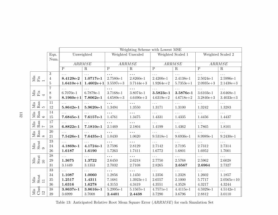
Weighting Scheme with Lowest MSEEqn.Num.
Unweighted Weighted Unscaled Weighted Scaled 1 Weighted Scaled 2
ARRMSE ARRMSE ARRMSE ARRMSEP R P R P R P R
Mis
Fix
1
3 . . . . . . . . . . . . . . . . . . . . . . . .4 8.4129e-2 1.0717e-1 2.7580e-1 2.8260e-1 2.4200e-1 2.4138e-1 2.5024e-1 2.5996e-15 1.6410e+1 1.4602e+1 3.5597e+3 3.7144e+3 1.9264e+2 5.7353e+1 2.0935e+3 2.1438e+3
Mis
Fix
4
7 . . . . . . . . . . . . . . . . . . . . . . . .8 6.7070e-1 6.7879e-1 3.7168e-1 3.8074e-1 3.5823e-1 3.5876e-1 3.6103e-1 3.6468e-19 8.1960e+1 7.8062e-1 4.6589e+3 4.6490e+3 4.6319e+2 4.6718e+2 3.2840e+3 3.4033e+3
Mis
Ran
5
11 . . . . . . . . . . . . . . . . . . . . . . . .12 5.8642e-1 5.9620e-1 1.3494 1.3550 1.3171 1.3100 1.3242 1.3283
Mis
Ran
6
14 . . . . . . . . . . . . . . . . . . . . . . . .15 7.6845e-1 7.6157e-1 1.4761 1.3475 1.4331 1.4335 1.4456 1.4437
Mis
Ran
7
17 . . . . . . . . . . . . . . . . . . . . . . . .18 6.8822e-1 7.1810e-1 2.1469 2.1804 1.4199 1.4362 1.7865 1.8101
Mis
Ran
8
20 . . . . . . . . . . . . . . . . . . . . . . . .21 7.5426e-1 7.6435e-1 1.0430 1.0620 9.5318e-1 9.6936e-1 8.9989e-1 9.2430e-1
Mis
Stra
t9
23 . . . . . . . . . . . . . . . . . . . . . . . .24 4.1869e-1 4.1724e-1 2.7596 2.8129 2.7142 2.7195 2.7312 2.731426 1.6187 1.6190 1.7263 1.7411 1.6772 1.6801 1.6952 1.7001
Mis
Stra
t10
28 . . . . . . . . . . . . . . . . . . . . . . . .29 1.3675 1.3722 2.6450 2.6218 2.7750 2.5768 2.5962 2.602831 3.1449 3.1353 2.7032 2.7108 2.8265 2.6567 2.6964 2.7327
Mis
Stra
t11
33 . . . . . . . . . . . . . . . . . . . . . . . .34 1.1087 1.0060 1.2856 1.1450 1.2356 1.2328 1.2602 1.185735 1.2517 1.4311 7.1681 1.3923e+1 2.6557 2.1000 5.7717 2.0565e+1036 1.6316 1.6278 4.3153 4.3419 4.3551 4.3528 4.3217 4.3244
Mis
Clu
st12
38 3.8637e-1 3.8616e-1 5.2995e-1 5.1567e-1 4.7571e-1 4.4115e-1 4.5929e-1 4.5142e-139 3.6999 3.7008 2.4401 2.4438 3.7290 3.6796 2.8812 3.0110
Table 13: Anticipated Relative Root Mean Square Error (ARRMSE) for each Simulation Set
132

8.5 Tables of True and Anticipated Parameter Values
For the computation of the ARRMSE values, the anticipated parameter values are needed.
The derivation of these values is in Section 8.1. They are also included in Tables 14 and
15 for reference.
133

True (Anticipated) Parameter ValuesEqn.Num.
β0 β1 β2 σ20k σ2
ε σ21k σ2
2k
Mis
Fix
1
3 1 -2 2 0.2 0.54 1(-5) -2 (NA) 2 (2) 0.2 (36.2) 0.5 (0.5)5 1(3) -2 (-2) 2 (NA) 0.2 (0.2) 0.5 (100.5)
Mis
Fix
4
7 1 -2 2 0.2 0.58 1(-5) -2 (NA) 2 (2) 0.2 (36.2) 0.5 (0.5)9 1(3) -2 (-2) 2 (NA) 0.2 (0.2) 0.5 (100.5)
Mis
Ran
5
11 1 -2 2 0.5 112 1(1) -2 (-2) 2 (2) 0 (18) 0.5 (0.5) 1(NA)
Mis
Ran
6
14 1 -2 2 0.5 115 1(1) -2 (-2) 2 (2) 0 (18) 0.5 (0.5) 1(NA)
Mis
Ran
7
17 1 -2 2 0.5 0.818 1(1) -2 (-2) 2 (2) 0 (1.6) 0.5 (16.5) 0.8(NA)
Mis
Ran
8
20 1 -2 2 0.5 0.821 1(1) -2 (-2) 2 (2) 0 (1.6) 0.5 (16.5) 0.8(NA)
Table 14: True and Anticipated Parameter Values for Simulation Sets 1-8.
True (Anticipated) Parameter ValuesEqn.Num.
β0 β1 σ201k σ2
02k σ201k.02k
13 σ2ε σ2
0k orσ2
0k1
σ20k1k2
orβ2
Mis
Stra
t9
23 -3 8 1 5 0 0.524 -3(1) 8 (NA) 1 (NA) 1 (NA) 0(NA) 0.5 (0.5) 0 (16)26 -3(1) 8 (NA) 1 (NA) 1 (NA) 0 (NA) 0.5 (0.5) 0 (16)
Mis
Stra
t10
28 -3 8 0.5 529 -3 (1) 8 (NA) 0.5 (16.5) 5 (5)31 -3 (1) 8 (NA) 0.5 (16.5) 5 (5)
Mis
Stra
t11
33 7 -8 1 5 0 0.5 -1034 7 (3) -8 (NA) 1 (NA) 5 (NA) 0 (NA) 0.5 (NA) 0 (0) -10 (-10)35 7 (2) -8 (-8) 1 (1) 5 (5) 0 (0) 0.5 (NA) -10 (NA)36 7 (-1) -8 (NA) 1 (NA) 5 (NA) 0 (NA) 0.5 (25.5) 0 (16.5) -10 (NA)
Mis
Clu
st12
38 5 (5) 0.5 (1.5) 5 (5) 1 (NA)39 5 (5) 0.5 (0.5) 5 (NA) 1 (6)
Table 15: True and Anticipated Parameter Values for Simulation Sets 9-12.
134

8.6 Computer Code
The simulations for PSHGR method were run using c-code I developed. This code may be
found at http://stat.cmu.edu under the Recent PhD Theses link. The c-code uses
the VMR library, downloaded from http://www.stat.cmu.edu/~hseltman/. It is in the
Computer Programming, C/C++ section. The code uses blas functions, downloadable
from http://www.netlib.org. The compilation instructions are commented in the begin-
ning of the code. Along with the code are sample input files and the corresponding output
file.
The simulations for the RHS method were run in stata using the gllamm() routine.
The gllamm() routine can be found at http://www.gllamm.org.
135

References
Asparouhov, T. (2006). General multi-level modeling with sampling weights. Communi-
cations in Statistics – Theory and Methods, 35:439 – 460.
Fienberg, S. E. (1989). Modeling considerations: Discussion from a modeling perspective.
In Kasprzyk, D., Duncan, G., Kalton, G., and Singh, M. P., editors, Panel Surveys,
pages 512–539. Wiley.
Hoem, J. (1989). The issue of weights in panel surveys of individual behavior. In Kasprzyk,
D., Duncan, G., Kalton, G., and Singh, M. P., editors, Panel Surveys, pages 512–539.
Wiley.
Huang, R. and Hidiroglou, M. (2003). Design consistent estimators for a mixed linear
model on survey data. In Proceedings of the Survey Research Methods Section, American
Statistical Association (2003), pages 1897–1904.
Kalton, G. (1989). Modeling considerations: Discussion from a survey sampling perspec-
tive. In Kasprzyk, D., Duncan, G., Kalton, G., and Singh, M., editors, Panel Surveys,
pages 575–585. Wiley.
Korn, E. L. and Graubard, B. I. (2003). Estimating variance components by using survey
data. Journal of the Royal Statistical Society, Series B, 65(1):175 – 190.
Little, R. (2004). To model or not to model? competing modes of inference for finite
population sampling. Journal of the Americal Statistical Association, 99:546–556.
Little, R. and Rubin, D. (2002). Statistical Analysis with Missing Data. Wiley.
Mislevy, R. J. and Sheehan, K. M. (1989). The role of collateral information about exam-
inees in item parameter estimation. Psychometrika, 54(4):661–679.
136

Patterson, B., Dayton, M., and Graubard, B. (2002). Latent class analysis of complex sam-
ple data: Application to dietary data. Journal of the American Statistical Association,
97(459):1–21.
Pfeffermann, D., Skinner, C., Holmes, D., Goldstein, H., and Rasbash, J. (1998). Weighting
for unequal selection probabilities in multilevel models. Journal of the Royal Statistical
Society, Series B, 60(1):23 – 40.
Rabe-Hesketh, S. and Skrondal, A. (2006). Multilevel modelling of complex survey data.
Journal of the Royal Statistical Society: Series A, 169:805–827.
Searle, S., Casella, G., and McCulloch, C. (1992). Variance Components. John Wiley &
Sons, Inc.
Stapleton, L. M. (2002). The incorporation of sample weights into multilevel structural
equation models. Structural Equation Modeling, 9(4):475–502.
Thomas, D. R. and Cyr, A. (2002). Applying item response theory methods to complex
survey data. In Proceedings of the Survey Methods Section, pages 17–25. Statistical
Society of Canada.
137
Related Documents