SAMPLING THEORY USING EXPERIMENTAL DESIGN CONCEPTS

SAMPLING THEORY 241

SAMPLING THEORY USING EXPERIMENTAL DESIGN CONCEPTS

Jaya Srivastava, Colorado State University

and

Zhao Ouyang, Colorado State University

Abstract

In this paper, we consider the application of concepts of StatisticalExperimental Design to Sampling Theory. As is well-known, because of itsinherent nature, Experimental Design Theory involves a relatively heavy amountof Combinatorial Mathematics. It turns out that, over the years, relativelyspeaking, it is this combinatorial aspect of Design, that has found muchapplication in Sampling. We present a brief review of the same, including someof the latest work in the field.

Introduction

The subject of sampling using experimental design concepts has attractedmore and more attention in recent years. A very explicit connection was madeby M.C. Chakrabarti (1963) who indicated that balanced incomplete blockdesigns (BIBD's) could be used as sampling schemes. At first, it was shown thata BIBD procedure has properties similar to SRSWOR (simple random samplingwithout replacement). But later on it was found that a BIBD corresponds, in asense, to controlled sampling, which was proposed by Goodman and Kish in 1950,and to which further contributions were made by Avadhani and Sukhatme (1965,1968, 1973).

Consider an agricultural survey. Suppose we use SRSWOR to draw asample of n counties from a population of N counties. It may happen that the ncounties in our sample are spread out in an undesirable or inconvenient manner.As pointed out by Avadhani and Sukhatme (1973), "this may not only increaseconsiderably the expenditure on travel, but the quality of data collected is alsolikely to be seriously affected by non-sampling errors, particularly non-responseand investigator bias, since in such cases organizing close supervision over thefield work would generally be fraught with administrative difficulties". Such a

sample is considered as non-preferred. Hence the total set of ί^J samples can be

classified into two classes: preferred samples and non-preferred samples(Goodman and Kish, 1950). Hence, our objective is to design a samplingprocedure which reduces the probability of drawing a non-preferred sample asmuch as possible, and at the same time resembles SRSWOR (assuming nostratification, clustering, etc. is present, and there are no auxiliary variables).

242 J. Srivastava &; Z. Ouyang

The problem of controlled sampling was first proposed by Goodman andKish (1950). This method involves stratified sampling and emphasizes theminimization of the probability of the selection of the non-preferred samples.But, as discussed by Avadhani and Sukhatme (1973), this method may loseprecision in estimation. In their three papers (1965, 1968, 1973), Avadhani andSukhatme discuss the problem of minimizing the chance of selection of non-preferred samples without losing efficiency relative to SRSWOR.

We recall some useful notation from Srivastava (1985). Let U denote apopulation with N units denoted by the integers 1, 2,...,7V. Let y be the variableof interest, and let yi (i = 1,.. .,7V) be the value of y for the unit i in U. Let Y =

J2 yi be the population total The class of all subsets of U is denoted by 2 , andTT

any ω G 2 is called a sample of U. (This includes the empty sample.) For anyset Ky let \K\ denote the number of elements in K. For any ω G 2 , let (ω:n) bethe class of all w-element subsets of u>; if |u>| < w, then this class is empty. Asampling measure, denoted by p( ), is a probability density {^(w)} defined on2U. For a given p( ), let

* ί = Σ P("), « = ! , . . . , # . (1)'6

Then, τrt (i = l,...,iV) is the probability that the unit i is included in the sample.For any non-empty sample ω, let ~yω denote the sample mean. Consider asampling measure p for which all inclusion probabilities iri (i = 1,...,JV) equal(n/N). Then, Avadhani and Sukhatme define p to be admissible if (i) Nyω is anunbiased estimator of 7, and (ii) Varp(Nyω) < VarSR^Nyω), where Varp andVarSRS denote the variance respectively under the measure p, and the measure qinduced by SRSWOR with sample size n. (Note that, for all ω G 2U, q(ω) =

n )}> ί f \ω\ = n ' a n d ί(ω) = °' otherwise.)

Let 3 < n < TV—3. The following results are given by Avadhani andSukhatme (1973).

Theorem 1

Let S C (U: n), and let \S\ = b. Then the sampling measure whichselects each ω G S with probability (1/6) is admissible if and only if |{α;: ω GS, i,j G w, i φ i}|, are the same for all % φ , ij = l,...,iV. For such ameasure, |{α;: ω G 5, % G w}| are the same for all i = 1,...,JV.

Under the condition of Theorem 1, let

λ = \{ω: ω G 5, t j e ω, i φ j}\ (2)

r = in/ΛΓ. (3)

SAMPLING THEORY 243

It is easy to see that the existence of S in Theorem 1 is equivalent to theexistence of a BIBD with parameters (N, b, r, n, λ), such that N is the number oftreatments, b the number of blocks, r the number of replications for eachtreatment, λ the number of blocks which contain any given pair of treatments,and n the block size. In fact, such a S is a BIBD with the above parameters.But, when N and n are large, such a BIBD may be hard to identify. So, the nexttwo theorems are useful.

Theorem 2

The measure induced by the following (two-part) sampling procedure isadmissible:

(i) Split the population randomly into k subpopulations with fixed sizes

N{ (i = 1,.. .,*) such that £ J\Γt = N,*=1

(ii) For t = 1,...,&, select ni units from the ith subpopulation by using anadmissible sampling measure (with inclusion probability {njN^)). Theselection of the units from the different subpopulations should be doneindependently.

Corollary 1

The measure induced by the following procedure is admissible:

(i) Draw a sample of size v! > n from the population by SRSWOR.

(ii) From the sample selected in (i), draw a sample of size n by using anadmissible measure with inclusion probability n/nf for each unit.

In view of the above, Avadhani and Sukhatme suggest that the followingsteps may be followed for controlled sampling:

(i) Let Nχ + N2 + ... + N_ = N. Divide the original populationrandomly into g subpopulations, which have sizes Nv JV2,..., J\Γrespectively.

(ii) Let nα + n2 + ... + ng = n. For i = 1, 2,...,<7, select an integer njsuch that nf < nj < Ni and also select a BIBD with parameters (τij ,δt , rt , niy λt ). (It is preferred that n{ be much smaller than n{ .) UseSRSWOR to select (independently for each i) a sample of size n{ fromthe i subpopulation of size N.

(iii) For each sample of size n\ (i = 1,..., ) drawn in step (ii), collect theinformation on all the preferred subsamples of size ni and then find a

244 J. Srivastava & Z. Ouyang

BIBD with parameters (nj, 6t , rt , ne-, λ4) such that the number of theblocks which correspond to the preferred subsamples of size nf is aslarge as possible. Then draw one block with probability l/bi from thei BIBD independently for i = 1,...,<7 In this way, we get a sampleof total size n^ + ... + n = n.

An example of controlled sampling using BIBD will be given in the lastsection in this paper.

Other Works on Sampling Using Concepts of Experiment Design

In the first section, we discussed the use of BIBD in controlled sampling.It is very clear that for a BIBD with parameters (N, δ, r, n, λ), N corresponds tothe number of units in the population, b corresponds to the (maximum possible)number of distinct samples, and n corresponds to the size of the sample. Withthis interpretation, it is easy to see that the parameters r and λ in the BIBDcorrespond respectively to the first order and the second order inclusion probabil-ities. So, for some time, the use of BIBD in sampling has been discussed widely.

As early as 1963, Chakrabarti pointed out the equivalence betweenSRSWOR and BIBD in the sense of having the same first order and second orderinclusion probabilities. It is clear that the smaller the support of (i.e., thenumber of distinct blocks in) the BIBD, the better is the possibility of adapting itfor a given situation of controlled sampling. Thus, BIBD's with a small supportsize have importance in sampling theory. Because of this, the work of Hedayatand others in the field of BIBD's with small supports is useful.

In 1977, Wynn showed that for each sampling measure p1 there is ameasure p2> which gives rise to the same first and second order inclusion proba-bilities as pv and whose support size is not greater than N(N - l)/2. For thecase of SRSWOR, he showed that no BIBD with support size less than N can beequivalent to SRSWOR in the above sense. Hence, with the help of BIBD's we

can reduce the support size from SRSWOR's ( JJ to something between ί ) andN.

Besides BIBD, Fienberg and Tanur (1985) listed some parallel conceptsin Design of Experiments and Sampling. These include randomization in designand random sampling, blocking in design and stratification in sampling, Latinsquare in design and lattice sampling, split-plot design and cluster sampling, andcovariance adjustment in design and post-stratification in sampling. By usingsome similar parallel concepts in design and sampling, Meeden and Ghosh (1983)found some admissible strategies in sampling and Cheng and Li (1983) showedthat Rao-Hartley-Cochran and Hansen-Hurwitz strategies are approximatelyminimax under some models. Brewer et al. (1977) discussed use of experimentaldesign in the planning of sample surveys, and Sedransk (1967) discussed the useof experimental design in the analysis of sample surveys. But, even thoughexperimental design and sampling have so many parallel concepts and similarstructure, sampling has been developed separately from experimental design.

SAMPLING THEORY 245

Smith and Snyder (1985) pointed out the main distinction between experimentaldesign and sampling from their nature of inference. They concluded that "thedifferences between survey and experiments are as important as the similarities,and that each will continue to develop in its own way". An excellent discussionof experimental design and sample surveys, both with respect to their similaritiesand differences, was given by Fienberg and Tanur (1985).

Hedayat (1979) gave a method for finding a sampling design which hasthe same first and second order inclusion probabilities, but has a reduced supportsize than SRSWOR. (In other words, he gave a general method for obtainingBIBD's with relatively small support sizes.) Let M denote the incidence matrixof all the pairs (i, j) versus all the samples of U with size n, where i, j £ U.

Thus, M is a ί (^) x (**) J zero-one matrix. Suppose all the samples of U with

size n are arranged in a list in an arbitrary but fixed order. Consider a BIBD(with block size n) in which fk denotes the frequency of the k sample in the

above list. Let / = (fv f2,...,./( „[)). Consider a sampling measure p which assigns

probability (/j./Σ/ί) to the * sample. Then, p has the same first and secondi

order inclusion probabilities as SRSWOR of size n iff Mf = λjL, where λ is apositive integer and I is a column vector with all entries equal to 1. So eachfeasible solution of the system

Mf=Xhf > 0 (4)

gives a sampling measure equivalent to SRSWOR of size n. Notice that there isalways a solution for the system. So we can introduce another quantity, forexample, the number of non-zero entries in /, and find a feasible solution of thesystem to minimize the quantity. The algorithm of mathematical programmingcan be used to get such a solution. In other papers in combinatorics, Hedayatand others give further results.

In Hedayat and Pesotan (1983), (R x L) triply balanced matrices wasdiscussed. The (R x L) triply balanced matrices arise in estimating the meansquare error of nonlinear estimators in sampling. Briefly, a (R x L) triply

Rbalanced matrix is Δ = (δ ) with entries +1 or -1 such that Σ# rA = 0,

R R J r=l

Σδrlfirs = 0» Y^^rhKJ^rt = > where the Λ, 5, t are distinct and A, 5, t = 1,...,Z.r=l r=l

It was proved that a (R x L) triply balanced matrix Δ is an orthogonal array ofstrength 3 and 2 symbols.

In Hedayat, Rao, and Stufken (1988), balanced sampling plans excludingcontiguous units are discussed. In some situations, the N units of the populationare arranged in a natural order. In this case it may happen that contiguous unitsprovides us similar information so that it seems more reasonable to select asampling plan such that the contiguous unit cannot appear in the sample. Here


the term balanced means that the first and second order inclusion probabilitiesare fixed. The condition of the existence of such a sampling measure is given inthis paper, and a method of constructing such a sampling measure is alsoproposed.

Use of i-Design

Suggested by the usefulness of BIBD with sampling, the use of /-design insampling was proposed by Srivastava and Saleh (1985). A BIBD, which has thesame inclusion probabilities (of individual units, and pairs of units) as SRSWOR,has the same moments as SRSWOR up to order two. Generalizing this,Srivastava and Saleh showed that a /-design has the same moments as SRSWORup to order /, because it has the same inclusion probabilities as SRSWOR up toorder / (i.e. every set of i units (i = 1,...,/) has the same inclusion probability,say gfj ). Also, as for the BIBD, the sample space under a /-design can be muchsmaller than the sample space under SRSWOR. Thus, using /-designs we can tryto avoid non-preferred samples, and still maintain resemblance to SRSWOR upto moments of order /.

For later use, define aiω (i G U, ω G 2U) by

aiω = 1, if i G ω

== 0, otherwise. (5)

Let 1 < k < N. For any sampling measure {/>(ω): ω G 2 } define

where t1? «2> Λ € UIn this section, we suppose the sample size is always equal to n, a fixed

integer. We are interested in estimating the population total Y.The following results from Srivastava and Saleh (1985) are useful in the

studies on using /-design theory in sampling.

Lemma 1

Let 2 < k < n. Suppose i j , . . . ,^ are distinct elements of U. Then wehave

]Γ>(h,...,*i) = ( n -

ik Φ «i,...,«,t_i (7)

(8)

SAMPLING THEORY 247

This lemma says that for 2 < k < n, the inclusion probabilities oforder j(l < j < k - 1) are determined by the inclusion probabilities of order k.

Theorem 3

Suppose there are two different sampling measures on 2 . Let < be apositive integer. Then these two sampling measures give the same inclusionprobabilities of order t if and only if these two sampling measures give the samevalues of E(y^), k = 1,..., t, for all possible values of (yv...,yj.

Let

11 ~ L i £ ω « - i -

Then, we have

Theorem 4

Consider two sampling measures on 2U. Consider the following fourconditions:

(i) For all possible values of y = (#!,...,yn);j E(jjJ) is the same under

these two sampling measures,

(ii) For all possible values of j/, E(ji2J), or E(s2J), or V(~yω) is the sameunder these two sampling measures,

(iii) For all possible values of j/, cov(Ίjω, s^) is the same under these twosampling measures,

(iv) For all possible values of j/, V(s2J) is the same under these twosampling measures.

Let ί be an integer such that 1 < t < 4. Then the above conditions (i), (ii), upto (i) are true if and only if these two sampling measures have the same inclusionprobabilities of order t

One can generalize Theorem 4 to higher order. But the most importantcase is order 4. In this case, we can characterize the mean and the variance of alinear estimator, and characterize the variance of a quadratic estimator of thevariance of the linear estimator.

Now consider a ί-design Z>(i\Γ, n, t, b) where N is the number of varieties,n the block size, b the number of blocks (which may or may not be distinct), and

where every combination of i varieties (t < u) occurs in δ(!f)/(w) blocks.


Consider a sampling measure (called a t~design sampling measure) which selects

each block of D(N, n, t, b) with probability 1/6. When b = (**) and each block

in DIN, n, ί, (^)J is distinct, this sampling measure becomes SRSWOR. In this

case SRSWOR is a /-design DyN, n, /, (^)J, where t can take any value from 1 to

n.For the /-design sampling measure mentioned above, for distinct iv...,it

G ί/, we have

•ft. > - KKHence we have the following theorem.

Theorem 5

SRSWOR (with sample size n) and the /-design sampling measure havethe same inclusion probabilities of order / and hence have the same moments upto order /.

For any /-design D(N, n, /, 6), the number of distinct blocks is not

greater than ( j , and usually is much less than ί ^ j . This makes a /-design useful

in controlled sampling. In fact, a BIBD is a 2-design. Because we need toestimate V(~yω), we need to consider up to the fourth moments; the first twomoments are not enough. In view of this, Srivastava and Saleh assert that itwould be much better to use 4-designs rather than BIBD's, since the former givesrise to the same moments as SRSWOR up to order 4.

Connection with Arrays

The theory of factorial designs constitutes a major part of the wholesubject of experimental design. Furthermore, the modern theory of factorialdesigns is largely built around the concept of arrays. Indeed, arrays constitute avery important tool in all of design theory, since for example, BIBD's, PBIBD'sand /-designs, etc. may (through their incidence matrices) be studied in terms ofarrays. Because of this, in this section, we discuss the application of arrays insampling theory. An array is a matrix whose elements come from a finite set.Suppose the finite set has m elements in it. Without loss of generality, we usethe integers 0, l,...,m-l to denote the elements of the finite set. In this case, anarray is a matrix whose elements belong to the set {0, l,...,ra-l}. When m = 2,such an array becomes (0, 1) matrix which is of special importance.

A special case of a (0, 1) matrix is the incidence matrix of a class ofsubsets of a given finite set. The rows of an incidence matrix correspond to theelements of the given finite set and the columns correspond to the subsets of thegiven finite set. In sampling, an incidence matrix is Ω^ which is a (N x 2^)(0, l)-matrix such that its columns correspond to the elements of 2 , and rows to

SAMPLING THEORY 249

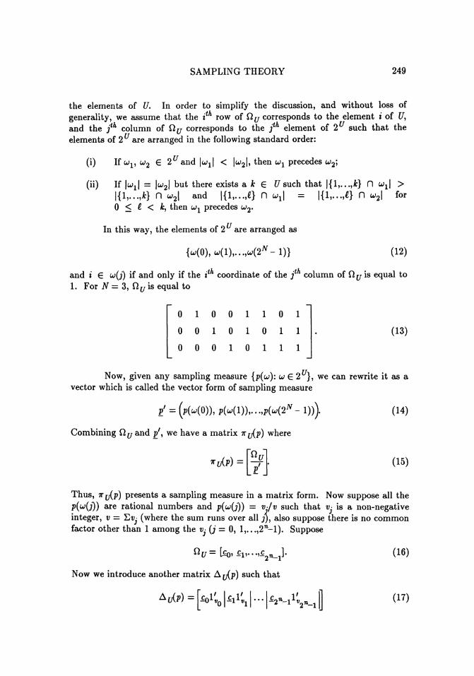
the elements of U. In order to simplify the discussion, and without loss ofgenerality, we assume that the ith row of Ω^ corresponds to the element i of U,and the j t h column of Ω^ corresponds to the j t h element of 2U such that theelements of 2 U are arranged in the following standard order:

(i) If ωv ω2 G 2^ and \ωχ\ < |u>2|, then ωχ precedes ω2,

(ii) If \ωλ\ = \ω2\ but there exists a k G U such that|{1,...,*} Π ω2\ and |{l,..,ί} \ |{0 < I < ifc, then ω1 precedes ω2.

ΓΊ ωχ\ =

In this way, the elements of 2 U are arranged as

} Π ωx\ >Π ω2\ for

(12)

and i E ω(j) if and only if the itfι coordinate of the j column of Ω^ is equal to1. For N = 3, Ω^ is equal to

0 1 0 0 1 1 0 1

0 0 1 0 1 0 1 1

0 0 0 1 0 1 1 1

(13)

Now, given any sampling measure {p(ω): ω G 2^}, we can rewrite it as avector which is called the vector form of sampling measure

p' = (K«(O)), p(ω(l)),...,p(ω(2N- 1))).

Combining Ωy and p', we have a matrix fl"y(p) where

(14)

(15)

Thus, 7Γ j^p) presents a sampling measure in a matrix form. Now suppose all thep(ω(j)) are rational numbers and p(ω(j)) = vjv such that Vj is a non-negativeinteger, v = Σv; (where the sum runs over all j), also suppose there is no commonfactor other than 1 among the i/ (j = 0, l,...,2n-l). Suppose

(16)

Now we introduce another matrix Δy(p) such that

(17)


where lf

k is the (1 x k) vector containing 1 everywhere, and where if for any j , wehave Vj = 0, then the columns (c) do not appear in Δ ^ p ) . Now, drawing acolumn from Δyζp) with probability (l/v) is equivalent to drawing a columnfrom Ω^ with probability measure {p(ω(j)) = v /v, j = 0, 1,...,2^-1}. So, thematrix Ay(p) represents the sampling measure in the form of an array and it iscalled sampling array in Srivastava (1988), wherein the following result is proved.

Theorem 6

For any vector form of sampling measure p and e > 0, there exists avector form of sampling measure /?* whose elements are rational such that(p ~ P*Y(p ~ P*) < t- (Note that every sampling measure can be expressed inthe vector form.)

Although this theorem seems simple it has an important interpretation inthat we can replace a sampling measure by a rational sampling measure asclosely as we want. On the other hand, by using a rational sampling measure weget a sampling array. So the above theorem connects sampling theory to thetheory of arrays in a fundamental manner, and hence to factorial and otherexperimental designs.

Now consider the problem of estimating the population total Y by ageneral linear estimator YQ (G means general), where

NYG = Σ Wi = Σ ciωaiωVi> ( 1 8 )

i € ω *=1

and where ciω are known real numbers which depend on i and ω for all i 6 U, ω£ 2U. Define

Φic= Σciωaiωp(ω) (19)

Φ°iic = Σ claiup(ω), φ% = Σ ciωcjωaiuajωP(ω) (20)

= Φc - ( W e + ΦΛN) + JNN (2 2)

where J m n is a m x n matrix which elements are equal to 1. It is easy to checkthat

Φ c = Σ K " ) U C U;

c (23)ω ω ω

where

ΰcω = (clωalω-^ C2ωa2ω-^' • ->cNωaNuΓl) ( 2 4 )

We have the following theorem:

SAMPLING THEORY 251

Theorem 7

The mean square error of ΫG as an estimator of Y denoted by MSE{ YG)is

MSE(ΫG)= Y*ΦCY. (25)

Notice that the matrix Φc is known when the sampling measure and theestimator ΫG are selected. The matrix Φc in sampling theory is similar to theinformation matrix in the theory of experimental design.

A General Estimator

In this section, we consider an estimator proposed in Srivastava (1985).There is an interesting history relevant here. First, in 1985, Srivastava observedthe connection between combinatorial arrays and sampling theory, discussed inthe last section. This appeared to open up a quite new theoretical field, in whichvariable sample size appeared to be inherent. Thus, there seemed to be a needfor a general estimator in which sample size was not necessarily fixed. Now,most estimators in sampling theory relate to fixed size. In many ways, the mostgeneral estimator (which, among other things, allows variable sample size)existing in 1985 was the Horvitz-Thompson estimator. But this is entirelydependent on the sampling measure, which is of course decided upon before thesample is drawn. In an attempt to be able to utilize the new knowledge(independent of the sample, but obtained during the course of actual sampling)the concepts of the sample weight function (discussed below), and the estimator ofthis section, were discovered. This estimator is extremely general, in that mostof the known estimators turn out to be its special cases.

The most important concept in this estimator is the introduction of thesample weight function r, defined on 2 , such that for all ω £ 2U, r(ω) is a finitereal number. For every K C U, and k £ (1, 2,...,iV), let

(K: k) = {ω:wC K, \ω\ = *}.

Clearly, if i £ (U: £), theni is a A -tuple, with k distinct elements from U. Fromhere on, Σ will denote the sum over all i_ £ (U: Jfc), Σ w m denote the sum

ί i_ίover all ω £ 2 u such that ± C ω, and Σ w m denote the sum over all i £

(w: k). Note that the last sum could be empty. In this section, we always lookuponi = (hv ••?*'*) as a n unordered set {ip. ••>**}• Let

M") (26)

For k G (1, 2,...,JV-1), t € (1, 2,...,JV), and i £ (U: k), let Γ r(j, t) bethe class of all unordered sets = (j0,...J^i) such that j G (U: t) and ± C j

252 J. Srivastava fe Z. Ouyang

wherei = (ij,...,^, and πjj) φ 0. Let

vj(i, t) = I Tr(i, Ol (27)

Also, let α(i, <) be real numbers which satisfy the following twoconditions:

a{i, t) = 0, if vjd, t) = 0, and (28)

Σ"U,<) = 1. (29)t=i

For all ω £ 2u,i e (U: *), define

(30)

where a~ = α"1 if a φ 0 and a~ = 0 if a = 0, and Σ* runs over all j G (U: t)such that i = (ί'lvi^jb) C i and j C ω. Now, consider the estimation of thefollowing symmetric linear population function Q(φ) where

Q(Φ) = ΣV-U). (31)I

where φ, defined over ({/: £), is such that for all ± G (U: k), ψ(J) is a realnumber. Notice when ± C ω and α; is selected, ^(i) can be calculated. Thus,once a sample ω is drawn, we can compute Qsr(ψ) where

)• (32)

Here in Q5r, 5 means that we are estimating a symmetric function, and r meansthat the sample weight function r is being used.

Theorem 8

The statistic Qsr(φ) is an unbiased estimator of Q(φ), if and only if forevery ± G (U: Jfc) with φ{i) φ 0, there exists a t such that 1 < t < N, ι/r(i, t)

φo.For the case of πr(i) φ 0 for all i G (U: Jfc), let a{χ, jfc) = 1 and α(i, /)

= 0 for all t φ k. Then we have

, ω) = K^KCi)]"1 a n d (33)

SAMPLING THEORY 253

(34)

By using Theorem 8, it can be checked that (34) is unbiased for Q(ψ)The variance of Qsr(φ) and an unbiased estimator of the variance of

Q8r{φ) were also obtained in Srivastava (1985). Now we turn to an estimator ofthe population total. N

Let k = 1, i = 1, φii) = Vi. Then Q{φ) = £ y. = Y. Then, (34) gives

(35)

By Theorem 8, if τrr(i) φ 0 for all i € U, then y s r l is an unbiased estimator ofY. When

r(ω) = 1, for all ω 6 2 ϋ , (36)

τrr(i)'s become π t 's where πi is the probability such that the unit i is included inthe sample. At this time, Ysrl becomes the well known Horvitz-Thompsonestimator ΫHT where

*/7Γ= ΣVi/*i (37)

The variance of Ϋsrl is given in the following theorem.

Theorem 9

Suppose πr(i) φ 0, i = l,...,i\Γ. Then

Σ Σ

where

•• # , J =

(38)

(39)

(40)


It is easy to see that

So the term in y\ in Var(Ϋsrl) is always larger than the correspondent term forYffT But we can choose r[ω) such that the cross product terms of Ϋ8rl are smallso that Var(Y8rl) is small. Examples are given in Srivastava (1985).

Balanced Array Sampling

We have defined arrays in the fourth section. Let K(a x b) andk(a x 1) be a matrix and a vector with elements from σβ, where σ8 is a finite setwhose elements are (0, 1,. ,.,s-l). The symbol λ( , ) is defined as a countingoperator, such that λ(&, K) is equal to the number of times k occurs as a columnof K. Let ψ8 be the permutation group over σ8. For φ G φ8, and j G σ5, letφ(j) be the image of .; when the permutation φ is applied. Similarly, we defineφ(k) = (φ(kί),...,φ(kβ)) iϊk= (kv...,ka) is a (α x 1) array over σ8.

Definition 1

Let K be a (a x b) array over σ8. Then K is a balanced array (B-array,or BA) of strength t if and only if

λ(*o, Ko) = λ {φ%), Ko) (42)

where kQ is any (i x 1) array over σ3, Ko is any (< x b) subarray of K and φ isany permutation in φ$.

Balanced arrays play an important role in factorial experimental designand coding theory. F o r i = (tp.. . ,^) € (U: fc), define

π(iv..., ik) = π(i)= Σ P H (43)ωl

When k = 1 or 2, the following customary notations will be used instead of 7r(i),

TΓ = τr(0, TΓ^ = π(2,;). (44)

Definition 2

Let p( ) = {p(ω): ω G 2^} be a sampling measure. Then p(-)corresponds to balanced array sampling wiih strength k iff π(i l v..,2^) is fixed, forall possible (iv...,ig) G (U: g). Here, g = 0, 1,...,*.

Thus, if p( ) corresponds to balanced array sampling with strength fc,then there exists θv...,θk such that

SAMPLING THEORY 255

*,(hv..,g = 0,, (45)

for (iv...,ig) e (U: g), and g = 0, 1,...,*.

Theorem 10

Suppose, the measure p( ) corresponds to BA sampling with strength k.Then there exists a sampling measure p*( ) whose sampling array is Δjy(/>*) suchthat Ay(p*) is a B-array of strength λ, and jp*( ) is arbitrarily close to p( ). (Inthe sense of Theorem 6.)

Theorem 11

Suppose Δ^p) is (N x v) B-array of strength L Let p( ) be a samplingmeasure such that it gives a probability (l/v) to each column of A^yip) f°Γ beingselected. Then p( ) corresponds to balanced array sampling with strength k.

Let <$! and δ2 be the mean and the variance of the sample size under themeasure p( ), i.e.,

δ2 = ΣKw)M (46)

(M - «i)2 (47)

Then we have the following theorem.

Theorem 12

Consider BA sampling whose inclusion probability is given by (45).Then

ΫHT=Θ-I

i\ω\yw (48)

V(ΫHT) = {(N-S^-^ + ψ r (49)

= £where Y = -ί]C !to ^ 2 = xr_ i £ ( ^ i ~ ^)2? a r e respectively of the population

mean and variance. (The significance of this result lies in the fact that if we havesome idea of the value of Y, we can reduce the variance below that of SRSWOR.This may happen, for example, in recursive sampling.)

256 J. Srivastava k Z. Ouyang

Definition 3

Let p( ) be a sampling measure. Then, p( ) corresponds to proportionalarray sampling with strength k (or, briefly, proportional sampling) iff for allinteger g such that 1 < g < fc, and all ( i l v > ϋ € (17: 0) we have

»(*!,...,*,) = *(h) •••*(*,)• (50)

Notice that when π t is fixed, say 6, for all i 6 ί7, then the proportionalarray sampling with strength k is also balanced array sampling with strength k. Inthis case we call it balanced proportional sampling with strength k.

In order to construct a p( ) which corresponds to proportional arraysampling with strength fc, we need the definition of orthogonal array (OA).

Definition 4

Let K be a (a x b) array over σ8. Then K is an orthogonal array ofstrength t if and only if

λ(*o, Ko) = b x 5"' (51)

where JCQ is any (t x 1) array over σ5, ϋΓ0 is any (t x 6) subarray of K. It iseasy to see that an OA with strength t is a BA with strength t.

Let L(N x b) = (€1,...r£jy)/ be an OA of strength ib over σ 5 where s is aprime number. Let st be an integer satisfying 1 < si < 5, i = 1,...,JV. In £{ ,replace the (sχ- - 1) symbols {2, 3,...,st } by 1, leave the original 1 unchanged, andreplace the other symbols (if any) by 0. Notice when si = 5, then the symbol si isthe same as symbol 0. Let L(N x b) be the array obtained by the abovereplacement.

Theorem 13

Consider a sampling measure p{ ) such that it has L(N x b) as asampling array. Then p( ) corresponds to proportional sampling of strength A;,such that the inclusion probability of unit i is equal to st /s, for i = l,...,i\Γ.

Theorem 14

We have

i=l

for proportional sampling and

var( ΫHT) = Q- - l ) [(N - 1> 2 + NΫ2]. (53)

for balanced proportional sampling.

SAMPLING THEORY 257

We can use BA sampling with strength 4 to imitate SRSWOR up to the4<A moments. Notice that the binomial sampling referred to in the literature, is abalanced proportional sampling with strength N. It is clear that it should be ade-quate enough to use balanced proportional sampling with strength 4 instead ofusing binomial sampling.

Weight Balanced Sampling

Now we introduce an estimator of Y called YΛ which is a special case ofΫsl when

r(ω) = M"1, for all u € 2U, ω φ φ. (54)

/ _ v- P(ω)aiω • , v /«*

w |u;|

(57)

where we assume that empty samples are not allowed.

Theorem 15

Suppose τr > 0 for i = 1,...,ΛΓ. Then

γ _ lwl~ ^ Y « lie1 (tJiλ

(59)

Notice that when the sample size is fixed, Ϋs2 = YJIJ

Definition 5

A sampling measure p( ) corresponds to weight-balanced (WB) sampling,if and only if (τr^/(τr^)2) and (TΓ /TΓJTΓ ) are constants for i G U and i φ , ij GU respectively.

258 J. Srivastava k Z. Ouyang

Let

< / ( * ί ) 2 = βv for all i (61)

<jl<*'i = β* for a 1 1 Φ h ij € ft (62)

We have the following corollary of Theorem 15.

Corollary 1

Under WB sampling, we have

V(Ki) = (N- l)S2(/?α - β2) + NΫ\βx - β2) + N(β2 - 1)]. (63)

Definition 6

A sampling measure p( ) corresponds to strongly weight-balanced (SWB)sampling if and only if πj, πf, π» are constants for i e U and i / j , ί j G ί7respectively.

Letπ{ = /?3 t€ 17, and (64)

/W\= Σ* (65)j

Theorem 16

For SWB sampling, we have

( ^ (66)

NSuppose q(n) > 0, n = l,...,iV and Σ ί( n) = l Suppose we draw a

n = l

sample in this way: firstly select the sample size n with probability #(π), thenuse SRSWOR to draw a sample of size n. Then use Nyω to estimate thepopulation total Y. In this way, we select a particular sample of size n with

probability q(n)/l ^J. We have

yJ = £ ύ4(Nyω - Y)21 \ω\ = n] (67)7 1 = 1 L J7 1 = 1

Σ7 1 — 1

SAMPLING THEORY 259

Hence, the technique of using Y52 to estimate the population total inSWB sampling is a technique which imitates SRSWOR.

An estimator YG is said to be location invariant if and only if

ΫG (given that y = y*) = -yQN + ΫG (given that y = y* + yo lJ\r) ( 6 8 )

ί N Vfor all real yQ, when y = (y^.-oίfiv)'' It is easy to see that YG = ί Σ ^iωaiωyi) ιs

N %=1

location invariant iff Σ ciωaiω = ^ f ° r a ^ w € 2 .t = l

Theorem 17

Under SWB sampling, Ys2 is location invariant.The material in this section comes from Srivastava (1987), where

examples of WB are given. From an unpublished paper of Srivastava andOuyang (1988), we know that Y52 is an admissible linear estimator of Y, and hasa variance formula which is similar to the Yates-Grundy variance formula forVar{ Ϋffγ) when the sample size is fixed.

An Example of Controlled Sampling and BA Sampling

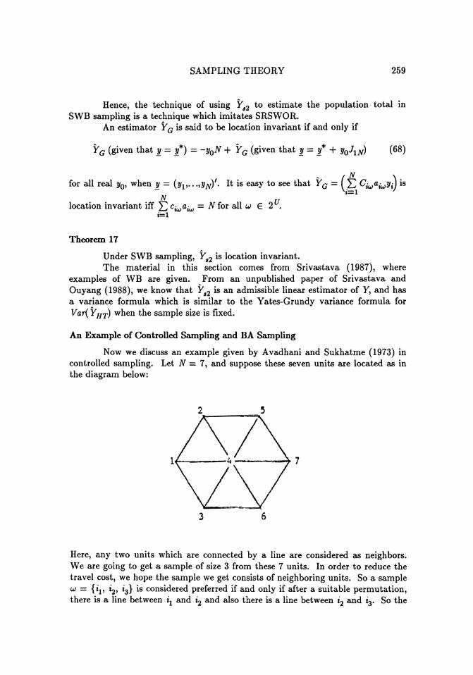
Now we discuss an example given by Avadhani and Sukhatme (1973) incontrolled sampling. Let N = 7, and suppose these seven units are located as inthe diagram below:

Here, any two units which are connected by a line are considered as neighbors.We are going to get a sample of size 3 from these 7 units. In order to reduce thetravel cost, we hope the sample we get consists of neighboring units. So a sampleω — i*v a2> 3} *s considered preferred if and only if after a suitable permutation,there is a line between iχ and i2 and also there is a line between i2 and i3. So the


total number of preferred samples is 21, and the total number of possible samples

is Q = 35.Consider a BIBD with parameter N= 7, A = 3, 6 = 7, r = 3, ι> = 1:

T =

2 2 3 1 3 1 1

5 4 6 4 4 2 5

7 6 7 7 5 3 6

(69)

Now only the block correspond to column 7 is not preferred. Hence if we useprobability 1/7 to draw a column from T, we reduce the probability of drawing anon-preferred sample greatly, and at the same time we have the same first twomoments as SRSWOR. But this technique does not avoid the nonpreferredsamples totally. To avoid the nonpreferred samples totally, consider a balancedarray approach as follows. We have a list of 16 samples: {147}, {246}, {543};{125}, {257}, {576}, {763}, {631}, {321}, {15}, {27}, {56}, {73}, {61}, {32};{5}. With probability (1/11) we draw any one of the first three samples, andwith probability (1/22) we draw any one of the remaining samples. Hence weavoid the nonpreferred samples. But we use some subsamples of the preferredsamples.

The problem of controlled sampling may be approached through theconcepts of array sampling as follows.

(i) Decide the preferred and nonpreferred samples.

(ii) Decide whether fixed sample size should be used or not.

(iii) Consider using BA sampling or WB sampling.

(iv) Suppose BA sampling is used. Then we need to find a BA whosecolumns consist of the preferred samples. If we fail to get such a BA,then consider subsamples of these samples. Sometimes we have tochange the decision in step (ii) to consider using some non-preferredsamples in this step (with minimal probability).

References

Avadhani, M. S. and Sukhatme, B. V. (1963): Controlled simple randomsampling, J. India Soc. Agricultural Stat. 17, 34-42.

Avadhani, M. S. and Sukhatme, B. V. (1967): Controlled sampling with varyingprobability with and without replacement, Austral. J. Siat. 9(1), 8-15.

SAMPLING THEORY 261

Avadhani, M. S. and Sukhatme, B. V. (1973): Controlled sampling with equalprobabilities and without replacement, International Stat. Review 41(2),175-182.

Brewer, K. R. W., Foreman, E. K., Mellor, R. W. and Trewin, D. J. (1977): Useof experimental design and population modelling in survey sampling,Bulletin of the International Stat Inst. 3, 173-190.

Brewer, K. R. W. and Hanif, M. (1983): Sampling with Unequal Probabilities,Springer-Verlag, New York, Heidelberg, Berlin.

Brunk, M. E. and Federer, W. T. (1953): Experimental designs and probabilitysampling in marking research, JASA 48, 440-452.

Cassel, C. M., Sarndal, C. E. and Wretman, J. H. (1977): Foundations ofInference in Survey Sampling, Wiley, New York.

Chakrabarti, M. C. (1963): On the use of incidence matrices of designs insampling from finite populations, J. Indian Stat. Soc. 1, 78-85.

Cheng, C. S. and Li, K. C. (1983): A minimax approach to sample surveys,Annals of Statistics 11, 552-563.

Cochran, W. G. (1977): Sampling Techniques, 3rd edition, Wiley, New York.

Cox, D. R. (1956): A note on weighted randomization, Annals of Math. Stat. 27,1144-1151.

Cox, D. R. (1958): Planning of Experiments, Wiley, New York.

Cumberland, W. G. and Royal, R. M. (1981): Prediction models and unequalprobability sampling, J. Roy. Stat. Soc, Ser. B, 43(3), 353-367.

Deming, W. E. (1953): On the distinction between enumerative and analyticsurvey, JASA 48, 244-255.

Dharmadhikari, S. W. (1982): Connectedness and zero variance in samplingdesigns, Stat. and Prob., 221-225.

Dwyer, P. S. (1972): Moment functions of sample moment functions, inSymmetric Functions in Statistics, ed. Derrick S. Tracy, University ofWindsor, Windsor, Ontario, 11-51.

Fellegi, I. P. (1963): Sampling with varying probabilities without replacement:Rotating and rotating samples, JASA 58, 183-201.


Kalton, G. (1983): Models in the practice of survey sampling, International Stat.Review 51, 175-188.

Kiefer, J. (1961): Optimum designs in regression problems. II, Annals of Math.Stat. 321, 298-325.

Kempthorne, O. (1952): The Design and Analysis of Experiments, Wiley, NewYork.

Kempthorne, O. (1955): The randomization theory of experimental inference,JASA 50, 946-967.

Kish, L. (1965): Survey Sampling, Wiley, New York.

Kruskal, W. H. and Mosteller, F. (1980): Representative sampling IV: Thehistory of the concept in statistics. 1815-1939, International Stat. Review48, 169-195.

Lacayo, H., Pereina, C. A. de, Proschan, F. and Sarndal, C. F. (1982): Optimalsample depends on optimality criterion, Scand. J. Stat. 9, 47-48.

Little, R. J. A. (1983): Estimating a finite population mean from unequalprobability sample, JASA 78(3), 596-604.

Lin, T. P. and Thompson, M. E. (1983): Journal of quadratic finite population:The batch approach, Annals of Stat. 11(1), 275-285.

Mahalanobis, P. C. (1944): On large-scale sample surveys, PhilosophicalTransactions of the Roy. Soc, London, 231(B), 329-451.

Meeden, G. and Ghosh, M. (1983): Choosing between experiments: Applicationsto finite population sampling, Annals of Stat. 11, 296-305.

Mikhail, N. N. and Ali, M. M. (1981): Unbiased estimates of the generalizedvariance for finite population, J. Indian Stat. Assoc. 19, 85-92.

Mukhopadhyay, P. (1975): An optimum sampling design to the HT method ofestimating a population total, Metrika 22, 119-127.

Mukhopadhyay, P. (1982): Optimal strategies for estimating the variance of afinite population under a superpopulation model, Metrika 29, 143-158.

Murthy, M. N.: Sampling theory and methods, Stat. Pub. Soc, Calcutta.

SAMPLING THEORY 263

Padmawar, V. R. (1981): A note on the comparison of certain samplingstrategies, J. Roy. Stat. Soc, Ser. B, 43(3), 321-326.

Pathak, P. K. (1964): On inverse sampling with unequal probabilities,Biometrika 51, 185-193.

Pereira, C. A. B. and Rodriques, J. (1983): Robust linear prediction in finitepopulations, International Stat. Review 51, 293-300.

Prasad, N. G. N. and Srivenkataramana, T (1980): A modification to theHorvitz-Thompson estimator under the Midzuno sampling scheme,Biometrika 67, 709-711.

Raj, D. (1958): On the relation accuracy of some sampling techniques, JASA 53,98-101.

Raj, D. (1972): Sampling Theory, McGraw-Hill Book Company, New York.

Ramakrisknan, M. K. (1975a): Choice of an optimum sampling strategy—I,Annals of Stat. 3(3), 669-679.

Ramakrishnan, M. K. (1975b): A generalization of the Yates-Grundy varianceestimator, Sankhya, Ser. C, 37, 204-206.

Rao, C. R. (1975): Some problems of sample surveys, Adv. Appd. Prob. 7(Supplement), 50-61.

Robinson, P M. (1982): On the convergence of the Horvitz-Thompson estimator,Austral. J. Stat. 24, 234-238.

Rosen, B. (1972): Asymptotic theory for successive sampling with varyingprobabilities without replacement I and II, Annals of Math. Stat. 43, 7, 373-392, 748-776.

Roy, J. (1957): A note on estimation of variance components in multistagesampling with varying probabilities, Sankhya 17, 367-372.

Rubin, D. B. (1978): Bayesian inference for causal effects: The role ofrandomization, Annals of Stat. 6, 34-58.

Sedransk, J. (1967): Designing some multi-factor analytical studies, JASA 62,1121-1139.


Srivastava, J. (1985): On a general theory of sampling, using experimentaldesign. Concept I: Estimation, Bulletin of International Stat. Inst., Vol.51, Book 2, 10.3-1 - 10.3-16.

Srivastava, J. (1988): On a general theory of sampling, using experimentaldesign. Concepts II: Relation with arrays, in Probability and Statistics, ed.J. N. Srivastava, North-Holland.

Srivastava, J. and Ouyang, Z. (1988a): Studies on the general estimator insampling theory, based on the sample weight function, unpublished paper.

Srivastava, J. and Ouyang, Z. (1988b): Optimal properties of balanced arraysampling and weight balanced sampling, unpublished paper.

Srivastava, J. and Saleh, F. (1985): Need of t-designs in sampling theory,Utilitas Mathematica 28, 5-17.

Stenger, H. and Gabler, S. (1981): On the completeness of the class of fixed sizesampling strategies, Annals of Stat. 9, 229-232.

Strauss, I. (1982): On the admissibility of estimators for the finite populationvariance, Metrika 29, 195-202.

Sukhatme, P. V. and Sukhatme, B. V. (1976): Sampling theory of surveys withapplications, New Dehli, Indian Soc. of Agricultural Stat.

Tepping, B. J., Hurvitz, W. N. and Deming, W. E. (1943): On the efficiency ofdeep stratification in block sampling, JASA 38, 93-100.

Vardeman, S. and Meeden, G. (1983): Admissible estimators in finite populationsampling employing types of prior information, JSPI7, 329-341.

Wilk, M. B. and Kempthorne, O. (1956): Some aspects of the analysis offactorial experiments in a completely randomized design, Annals of Math.Stat. 27, 950-985.

Wynn, H. P. (1976): Optimum designs for finite populations sampling, inStatistical Decision Theory and Related Topics, eds. S. S. Gupta and D. S.Moore, Academic Press, New York.

Wynn, H. P. (1977a): Minimax purposive survey sampling design, JASA72(359), 655-657.

Wynn, H. P. (1977b): Convex set of finite population plans, Annals of Stat. 5,414-418.

SAMPLING THEORY USING EXPERIMENTAL DESIGN CONCEPTS

Documents