Sampled Medial Loci and Boundary Differential …shape/publications/3dim09.pdfSampled Medial Loci and Boundary Differential Geometry ... ple of points on the medial locus of a polyhedral

Sampled Medial Loci and Boundary Differential Geometry

Svetlana StolpnerSchool of Computer Science

McGill UniversityMontreal, QC, [email protected]

Sue WhitesidesDepartment of Computer Science

University of VictoriaVictoria, BC, Canada

[email protected]

Kaleem SiddiqiSchool of Computer Science

McGill UniversityMontreal, QC, [email protected]

Abstract

We introduce a novel algorithm to compute a dense sam-ple of points on the medial locus of a polyhedral object,with a guarantee that each medial point is within a speci-fied tolerance ε from the medial surface. Motivated by Da-mon’s work on the relationship between the differential ge-ometry of the smooth boundary of an object and its medialsurface [8], we then develop a computational method bywhich boundary differential geometry can be recovered di-rectly from this dense medial point cloud. Experimental re-sults on models of varying complexity demonstrate the va-lidity of the approach, with principal curvature values thatare consistent with those provided by an alternative methodthat works directly on the boundary. As such, we demon-strate the richness of a dense medial point cloud as a shapedescriptor for 3D data processing.

1. Introduction

The ubiquity of polyhedral models in computer vision,computer graphics, medical imaging and solid modelingcalls for algorithms for the analysis of the smooth objectboundaries associated with them. Medial representations,introduced in [3], have found useful applications in thiscontext, including object recognition and retrieval, objectsegmentation, object registration, statistical shape analysis,motion planning, object animation and path planning [19].Strikingly, whereas the majority of these applications use amodel comprised of medial points and their spoke vectors,few (if any) have capitalized on the fact that these quantitiessuffice to recover the differential geometry of the impliedboundary.

In this article, we present:

1. A novel algorithm to obtain a dense set of points withina one-sided Hausdorff distance ε of the object’s medialsurface, along with their spoke vectors in Section 3.Medial surface normals are then computed from the

spoke vectors, following which the medial point cloudmay be segmented into its constituent smooth sheets.

2. A novel algorithm to obtain the principal curvaturesand principal curvature directions of the two impliedboundary patches on either side of each medial point inSection 5. These curvature estimates are then mappedonto the polyhedral object boundary B.

These results are the first computational investigations,to our knowledge, which relate medial differential geometryto boundary differential geometry for arbitrary polyhedralmodels. We demonstrate that a discrete approximation tothe medial surface is sufficient to estimate local differentialproperties of the object boundary.

2. Background and Related Work

We begin with an overview of medial surfaces and theirproperties. Consider a solid object Ω with boundary B.

Definition 1 The medial surface MS of Ω is the locus ofcentres of all maximal spheres inscribed in Ω.

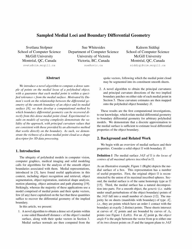
As an illustrative example, Figure 1 (Right) depicts the me-dial surface of a box. This representation has a numberof useful properties. First, the original object Ω is recon-structed by the union of its maximal inscribed spheres. Sec-ond, the medial surface is of the same homotopy type as Ω[15]. Third, the medial surface has a natural decomposi-tion into parts. For a smooth object, the generic (i.e. stableunder small perturbations of the object boundary) points oftheMS fall into a small number of classes [12]. The ma-jority lie on sheets (manifolds with boundary) of type A2

1,i.e., they are points which have an order-1 contact with theboundary at exactly 2 distinct points. These sheets intersectat curves of A3

1 points and are bounded by curves of A3

points (see Figure 1 (Left)). For an A21 point p, the object

angle θ is the angle between the vector from p to either oneof its two closest points on B and the tangent plane toMS

Figure 1. Left: Different classes of points that compose the mediallocus of a smooth 3D object [12]. Right: The medial surface of abox, with each sheet shown in a different colour. The object angleθ at the selected medial point is π/4. The spoke vectors are theblack arrows.

at p (see Figure 1 (Left)). We shall refer to the vectors fromp to its two closest points on B as the spoke vectors.

When Ω is a polyhedron,MS is composed of bisectorsof the faces, edges and vertices of B. The bisector of twosuch elements is a quadric surface and these surfaces inter-sect along curves of higher algebraic degree. Thus, the com-plete medial surface of a polyhedron can be complex and isimpractical (and often unnecessary) to compute exactly formodels with a large number of faces. A common strategy,therefore, is to only recover those parts of the medial surfacewhich are “salient” with respect to an appropriate measure,such as the associated object angle [19].

2.1. Medial Surface Computation

A variety of methods have been proposed for computingmedial surfaces of polyhedral models. Amenta et al. [1] ap-proximate the medial surface by a subset of the Voronoi ver-tices, the ‘poles’, of points sampled on the object’s surface.Leymarie and Kimia [14] compute a geometric directed hy-pergraph whose nodes are medial points, using exact bisec-tor computations between clusters of surface points. Culveret al. [7] use exact arithmetic to compute the seams of themedial surface of polyhedra having a small number of faces.Etzion and Rappaport [10] perform spatial subdivision un-til each cell contains one vertex of the generalized Voronoidiagram of a polyhedron. Foskey et al. [11] approximatethe medial surface of a mesh having a chosen object anglewith axis-aligned facets, with computations accelerated bygraphics hardware.

We now specialize to methods for computing the medialsurface that are based on the average outward flux of thegradient of the Euclidean distance transform of the objectΩ. This approach is well suited to our goal of recoveringboundary differential geometry directly from medial geom-etry as, in this framework, it is possible to efficiently and ac-

curately compute a dense collection of medial points alongwith their spoke vectors.

Definition 2 The Euclidean distance transform of a solidΩ with boundary B is given by D(p) = infq∈B d(p,q),where p ∈ Ω and d(p,q) denotes Euclidean distance.

∇D : R3 → R3 is hence a unit vector field where eachpoint in the interior of Ω is assigned the direction from theclosest point on B, which is also an inward normal to B.The following useful relationships between the average out-ward flux AOF of ∇D through a sphere S inside Ω withoutward normal NS and medial sheets in S are shown in[20]. If no medial sheet passes through S,

limarea(S)→0

AOF = limarea(S)→0

∫∫S∇D ·NSdS∫∫

SdS

= 0. (1)

However, if a medial sheet with object angle θ passesthrough S,

limarea(S)→0

∫∫S∇D ·NSdS∫∫

SdS

= −12

sin(θ). (2)

We wish to apply the above continuous criterion to detectregions of space inside B that contain medial points. To dothis, we voxelize the interior of B and circumscribe eachvoxel with a sphere S. We then sample m points pi on thesurface of S. A discrete version of AOF then is:

AOF =∑mi=1∇D(pi) ·NS(pi)

m. (3)

Eqs. 1 and 2 require that the area of S shrinks to zero. WhenS is of non-zero size andB is the boundary of a polyhedron,[20] shows that if the contribution of certain sample pointspi to the sum in Eq. 3 is ignored, then the quantity AOF is0 if there are no medial points and proportional to the objectangle of the medial points inside S otherwise.

2.2. Discrete Differential Geometry

The traditional approach to estimating curvatures on ob-jects represented as triangle meshes is to perform compu-tations directly on the boundary [17]. These methods maybe divided into two classes: those that fit analytic functionsto the data and those that work with the discrete data di-rectly. In the former class, Cazals and Pouget [4] show thatdifferential quantities evaluated for fitted polynomial sur-faces of required degree converge to the true values giventhat a sampling condition on the boundary is met. In thelatter class, Taubin [22] finds curvature tensors by consid-ering estimates of normal curvature in a neighbourhoodabout each mesh vertex. The curvature values obtainedfrom the curvature tensor in [6] approach the true valuesif a sampling condition on a particular kind of mesh is sat-isfied. Rusinkiewicz [18] performs this computation on a

per-triangle basis. The work of Taubin [22] is extended to3D range data in [13].

The method that we develop for recovering boundary dif-ferential geometry in this paper is fundamentally differentfrom the above techniques since it relies on medial geom-etry. In fact, to our knowledge there is very little com-putational work relating medial geometry to boundary ge-ometry, with two exceptions. In [16] formulas are derivedfor the Gaussian and Mean curvatures for 3D boundariesbased on derivatives along medial sheets, but this theoryhas not yet lead to implementations. For objects with non-branching medial topology, Yushkevich et al. [23] fit asingle-sheet continuous medial representation (an m-rep) tomedical image data and derive conditions to compute theimplied boundary.

3. Dense and Precise Medial PointsAs a starting point, we use the method of [20] to com-

pute a set of voxels inside a polyhedral object Ω that areintersected by the medial surface. In this section, we showhow these initial estimates can be refined to give a densemedial point cloud with a precision guarantee.

3.1. Precise Medial Point Location

We first describe a subroutine that uses informationabout the gradient of the Euclidean distance transform tolocate points near the medial surface. Let (a,b) be a linesegment connecting points a and b. The subroutine is basedon the following lemma proved in [21]:

Lemma 1 Let p be a point in Ω. Let q = p + γ · ∇D(p),such that q is also in Ω and γ is a scalar. A medial point ofΩ lies on (p,q) if and only if∇D(p) 6= ∇D(q).

Algorithm 1 RETRACT(p,q, ε)Input: Points p,q inside Ω s.t. q = p + γ · ∇D(p) and∇D(p) 6= ∇D(q), tolerance ε.

Output: A point within ε of the medial surface of Ω and itstwo spoke vectors.

1: while d(p,q) > ε do2: m = 1

2 (p + q)3: if ∇D(m) 6= ∇D(p) then4: q = m5: else6: p = m7: end if8: end while9: Return p,∇D(p), ∇D(q).

By Lemma 1, Algorithm 1 finds a point on (p,q) thatis within a user-specified tolerance ε of the medial surface

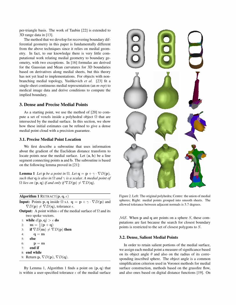
Figure 2. Left: The original polyhedra; Centre: the union of medialspheres; Right: medial points grouped into smooth sheets. Theallowed tolerance between adjacent normals is 5.7 degrees.

MS. When p and q are points on a sphere S, these com-putations are fast because the search for closest boundarypoints is restricted to the set of closest polygons to S.

3.2. Dense, Salient Medial Points

In order to retain salient portions of the medial surface,we assign each medial point a measure of significance basedon its object angle θ and also on the radius of its corre-sponding inscribed sphere. The object angle is a commonsimplification criterion used in Voronoi methods for medialsurface construction, methods based on the grassfire flow,and also ones based on digital distance functions [19]. On

Model # Triangles Final Voxel # Medial TimeResolution Points (min)

Torus 16,000 3,033,136 64,195 5.93Pear 86,016 5,177,526 18,147 22.24Head 6,816 5,244,401 74,853 6.22Venus 22,688 7,739,924 116,793 12.82

Table 1. Statistics for the computation of medial points.

the other hand, Chazal and Lieutier [5] prove that a simpli-fication scheme based on radius preserves topology. Attaliet al. [2] argue in favour of a simplification scheme basedon both object angle and radius.

Our algorithm for detecting salient medial points is asfollows. For each voxel u that is known to contain me-dial points, we attempt to find a salient medial point insideu. For each of the sample points p on the circumscribingsphere S of u, we check to see if∇D(p) 6= ∇D(q), whereq 6= p is a point of intersection of the ray p − ∇D(p)with S. If so, Algorithm 1 finds an approximate locationof a medial point x along the segment (p,q), as well as its2 spoke vectors. Note that the spoke vector ∇D(p) is ex-act, while ∇D(q) is approximate. The object angle is thenhalf the angle between these spoke vectors and the radius istheir magnitude. Point x returned by Algorithm RETRACTis stored as the medial point associated with voxel u if xlies inside voxel u and if either the object angle or radiusthreshold is satisfied. At most one medial point is found pervoxel. Thus, the density of the medial points is controlledby the resolution of the voxels considered. Deciding if avoxel contains a salient medial point is done quickly by us-ing efficient point to polygon mesh distance tests and takingadvantage of temporal coherence between queries. Hence,we can choose a fine resolution that produces a large num-ber of voxels.

Figure 2 (Centre) illustrates the union of the maximalspheres for the computed medial points with object anglethreshold 0.3 radians and radius threshold 0.25 times themaximum dimension of the bounding box. These examplesshow that the boundary of the union of spheres associatedwith the salient medial point cloud provides a close visualapproximation to the boundary B of the original object.

Statistics for the computation of medial points for themodels shown in this paper are given in Table 1. The finalvoxel resolution is the number of finest-resolution voxelsin the interior of the model. The number of medial pointsis the number of salient medial points found, at most oneper finest-resolution voxel. Timings are shown for a sin-gle 3.4GHz Pentium IV processor with 3GB of RAM. Notethat our code can easily be parallelized to speed up compu-tations.

3.3. Medial Surface Normals

Given a medial point x0 and its two spoke vectors Uax0

and Ubx0

, these vectors make an equal angle with the tangentplane toMS at x0, Tx0MS. We use this fact to derive theequation for the normal N(x0) to Tx0MS as follows. Forx ∈ Tx0MS,

Ua(x0) · (x0 − x) = Ub(x0) · (x0 − x) (4)

⇒ (Ua(x0)−Ub(x0)) · (x0 − x) = 0. (5)

Therefore, Ua(x0) − Ub(x0) is the normal direction toTx0MS . Figure 2 shows the polyhedra (Left) and theirmedial surfaces (Right) computed by our algorithm. Weillustrate the quality of the normal estimates by groupingmedial points that have locally consistent normals. Specif-ically, for a medial point q on a sheet that is inside voxeluq, we add to this sheet all medial points p inside voxels inthe 26-neighbourhood of uq whose normals are within anallowed tolerance of the normal at p. The result is a seg-mentation of the medial surface into smooth sheets of A2

1

points.

4. Boundary Geometry from Medial GeometryThe work of Damon [8] demonstrates that surface dif-

ferential geometry can be directly inferred from the rate ofchange of the spoke vectors with respect to the medial sur-face. In this section, we survey some of the results in [8].

IfB ⊂ R3 is the boundary of an object Ω ⊂ R3 with unitoutward normals n, then the rate of change of n along Bdescribes the curvature of B. Rather than studying the rateof change of n as one moves along B, consider the rate ofchange of n as one moves along medial surfaceMS of Ω.Recall that smooth (A2

1) medial points are equidistant fromexactly 2 points on B. The vectors from smooth medialpoints to nearest points on B, the spoke vectors, are normalto B. Thus, by studying the rate of change of the spokevectors we obtain information about the rate of change ofthe normals to the boundary.

Consider a smooth medial point x0 ∈ MS and letUa,Ub be the 2 spoke vectors at x0. Let Ua

1 =Ua/‖Ua‖,Ub

1 = Ub/‖Ub‖. Damon defines

Sarad(v) = −projUa(∂Ua

1

∂v) and (6)

Sbrad(v) = −projUb(∂Ub

1

∂v), (7)

where projU denotes projection into Tx0MS along U [8].Refer to Figure 3.

Choosing an orthonormal basis v1,v2 for Tx0MS,let Sarad, Sbrad denote the matrix representation of the tworadial shape operators. Then, as in the case of the stan-dard shape operator, the eigenvectors are principal radial

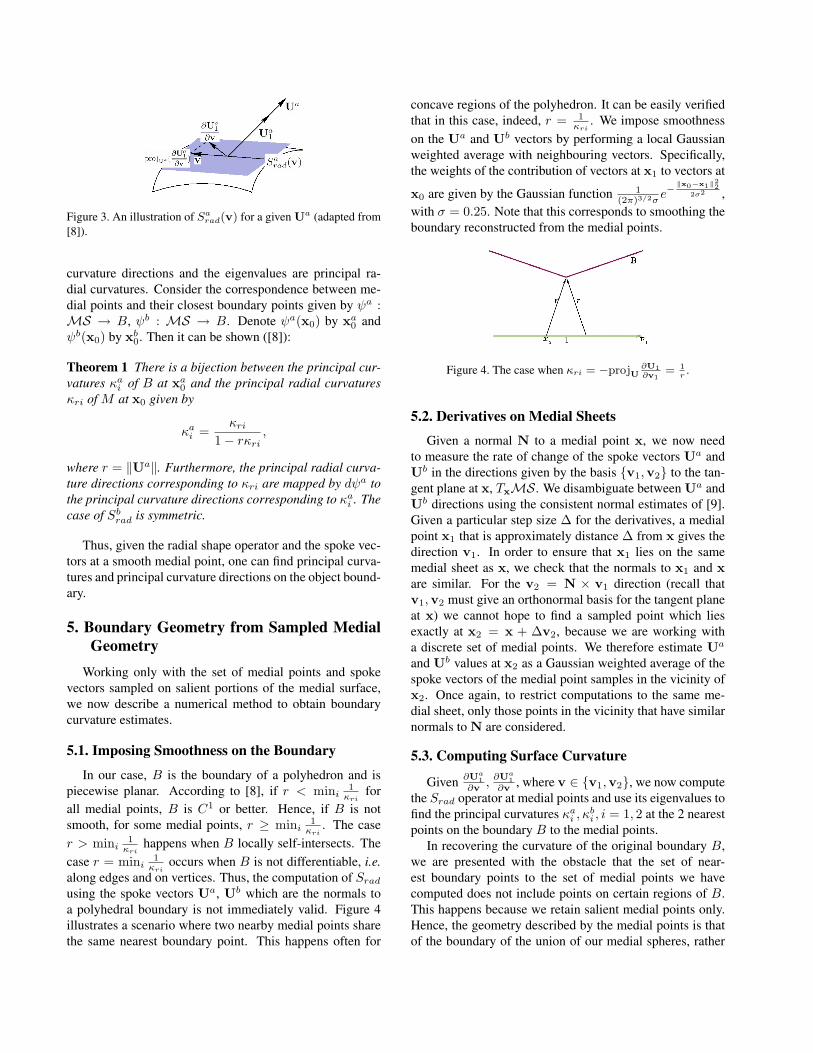
Figure 3. An illustration of Sarad(v) for a given Ua (adapted from

[8]).

curvature directions and the eigenvalues are principal ra-dial curvatures. Consider the correspondence between me-dial points and their closest boundary points given by ψa :MS → B, ψb : MS → B. Denote ψa(x0) by xa0 andψb(x0) by xb0. Then it can be shown ([8]):

Theorem 1 There is a bijection between the principal cur-vatures κai of B at xa0 and the principal radial curvaturesκri of M at x0 given by

κai =κri

1− rκri,

where r = ‖Ua‖. Furthermore, the principal radial curva-ture directions corresponding to κri are mapped by dψa tothe principal curvature directions corresponding to κai . Thecase of Sbrad is symmetric.

Thus, given the radial shape operator and the spoke vec-tors at a smooth medial point, one can find principal curva-tures and principal curvature directions on the object bound-ary.

5. Boundary Geometry from Sampled MedialGeometry

Working only with the set of medial points and spokevectors sampled on salient portions of the medial surface,we now describe a numerical method to obtain boundarycurvature estimates.

5.1. Imposing Smoothness on the Boundary

In our case, B is the boundary of a polyhedron and ispiecewise planar. According to [8], if r < mini 1

κrifor

all medial points, B is C1 or better. Hence, if B is notsmooth, for some medial points, r ≥ mini 1

κri. The case

r > mini 1κri

happens when B locally self-intersects. Thecase r = mini 1

κrioccurs when B is not differentiable, i.e.

along edges and on vertices. Thus, the computation of Sradusing the spoke vectors Ua, Ub which are the normals toa polyhedral boundary is not immediately valid. Figure 4illustrates a scenario where two nearby medial points sharethe same nearest boundary point. This happens often for

concave regions of the polyhedron. It can be easily verifiedthat in this case, indeed, r = 1

κri. We impose smoothness

on the Ua and Ub vectors by performing a local Gaussianweighted average with neighbouring vectors. Specifically,the weights of the contribution of vectors at x1 to vectors at

x0 are given by the Gaussian function 1(2π)3/2σ

e−‖x0−x1‖

22

2σ2 ,with σ = 0.25. Note that this corresponds to smoothing theboundary reconstructed from the medial points.

Figure 4. The case when κri = −projU∂U1∂v1

= 1r

.

5.2. Derivatives on Medial Sheets

Given a normal N to a medial point x, we now needto measure the rate of change of the spoke vectors Ua andUb in the directions given by the basis v1,v2 to the tan-gent plane at x, TxMS . We disambiguate between Ua andUb directions using the consistent normal estimates of [9].Given a particular step size ∆ for the derivatives, a medialpoint x1 that is approximately distance ∆ from x gives thedirection v1. In order to ensure that x1 lies on the samemedial sheet as x, we check that the normals to x1 and xare similar. For the v2 = N × v1 direction (recall thatv1,v2 must give an orthonormal basis for the tangent planeat x) we cannot hope to find a sampled point which liesexactly at x2 = x + ∆v2, because we are working witha discrete set of medial points. We therefore estimate Ua

and Ub values at x2 as a Gaussian weighted average of thespoke vectors of the medial point samples in the vicinity ofx2. Once again, to restrict computations to the same me-dial sheet, only those points in the vicinity that have similarnormals to N are considered.

5.3. Computing Surface Curvature

Given ∂Ua1

∂v ,∂Ua

1∂v , where v ∈ v1,v2, we now compute

the Srad operator at medial points and use its eigenvalues tofind the principal curvatures κai , κ

bi , i = 1, 2 at the 2 nearest

points on the boundary B to the medial points.In recovering the curvature of the original boundary B,

we are presented with the obstacle that the set of near-est boundary points to the set of medial points we havecomputed does not include points on certain regions of B.This happens because we retain salient medial points only.Hence, the geometry described by the medial points is thatof the boundary of the union of our medial spheres, rather

than that of the original boundary B. For medial points thatcontribute a large spherical patch to the reconstruction ofthe shape, we only have curvature information about its 2nearest boundary points (refer to Figure 5 for a 2D illus-tration). These points correspond to A3 points in Giblinand Kimia’s classification[12], or ‘edge points’ (see Figure1 (Left)). Surface curvature values at missing locations arecomputed by propagating known surface curvature valuesof neighbouring surface points along the boundary B.

Figure 5. The medial surface of this object consists of low-objectangle segments (dashed lines) and a high-object angle segment(bold line). When approximating the medial surface with a setof points, we only retain points on high-object angle segments ofthe medial surface. The boundary of the union of the associatedmedial circles approximates the original object. Medial pointm isequidistant from points A and B on the boundary. Surface curva-tures at points A and B are found using the radial shape operator,while for point C a different strategy is used.

6. Experimental ResultsWe present numerical results on polyhedral objects of

varying topology and surface complexity, and with vary-ing medial surface branching topology: a three-hole torus,a pear, a head, and a Venus model.1 To show surface cur-vatures, we use the colormap in Figure 6 (Bottom Right).Here, red corresponds to a convexity, blue to a concav-ity, green to a saddle-shaped region, yellow to a cylindri-cal patch curving toward the object (the non-zero principalcurvature is positive), cyan to a cylindrical patch curvingaway from the object (the non-zero principal curvature isnegative) and white to a flat region. Figure 6 (Left) showsthe surface curvature estimates on the medial surface andFigure 6 (Middle) shows these estimates projected onto theboundary B. For comparison, Figure 6 (Right) shows theresult of applying Rusinkiewicz’s method [18] directly onB.

Although there are subtle numerical differences, the re-sults obtained by the two methods are qualitatively veryconsistent. We emphasize that the implementation of our

1Models from the Princeton Shape Benchmark, http://vcg.isti.cnr.it/polycubemaps/models/, and http://www.cs.princeton.edu/gfx/proj/sugcon/models/

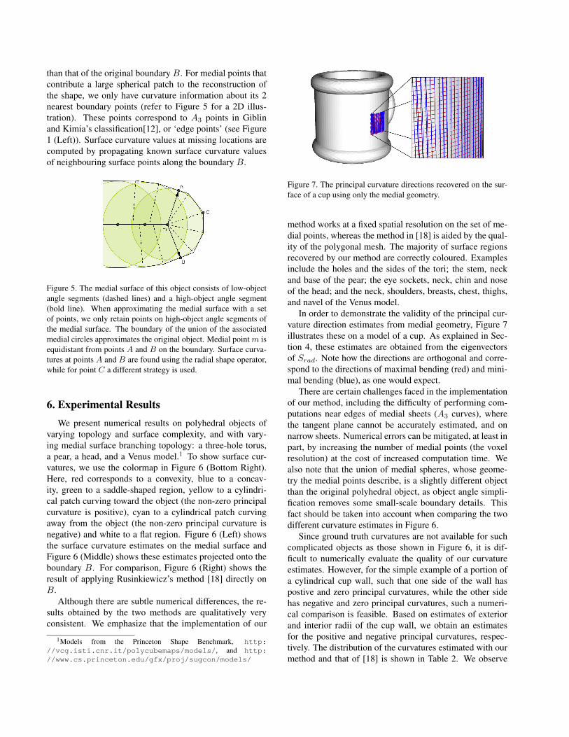
Figure 7. The principal curvature directions recovered on the sur-face of a cup using only the medial geometry.

method works at a fixed spatial resolution on the set of me-dial points, whereas the method in [18] is aided by the qual-ity of the polygonal mesh. The majority of surface regionsrecovered by our method are correctly coloured. Examplesinclude the holes and the sides of the tori; the stem, neckand base of the pear; the eye sockets, neck, chin and noseof the head; and the neck, shoulders, breasts, chest, thighs,and navel of the Venus model.

In order to demonstrate the validity of the principal cur-vature direction estimates from medial geometry, Figure 7illustrates these on a model of a cup. As explained in Sec-tion 4, these estimates are obtained from the eigenvectorsof Srad. Note how the directions are orthogonal and corre-spond to the directions of maximal bending (red) and mini-mal bending (blue), as one would expect.

There are certain challenges faced in the implementationof our method, including the difficulty of performing com-putations near edges of medial sheets (A3 curves), wherethe tangent plane cannot be accurately estimated, and onnarrow sheets. Numerical errors can be mitigated, at least inpart, by increasing the number of medial points (the voxelresolution) at the cost of increased computation time. Wealso note that the union of medial spheres, whose geome-try the medial points describe, is a slightly different objectthan the original polyhedral object, as object angle simpli-fication removes some small-scale boundary details. Thisfact should be taken into account when comparing the twodifferent curvature estimates in Figure 6.

Since ground truth curvatures are not available for suchcomplicated objects as those shown in Figure 6, it is dif-ficult to numerically evaluate the quality of our curvatureestimates. However, for the simple example of a portion ofa cylindrical cup wall, such that one side of the wall haspostive and zero principal curvatures, while the other sidehas negative and zero principal curvatures, such a numeri-cal comparison is feasible. Based on estimates of exteriorand interior radii of the cup wall, we obtain an estimatesfor the positive and negative principal curvatures, respec-tively. The distribution of the curvatures estimated with ourmethod and that of [18] is shown in Table 2. We observe

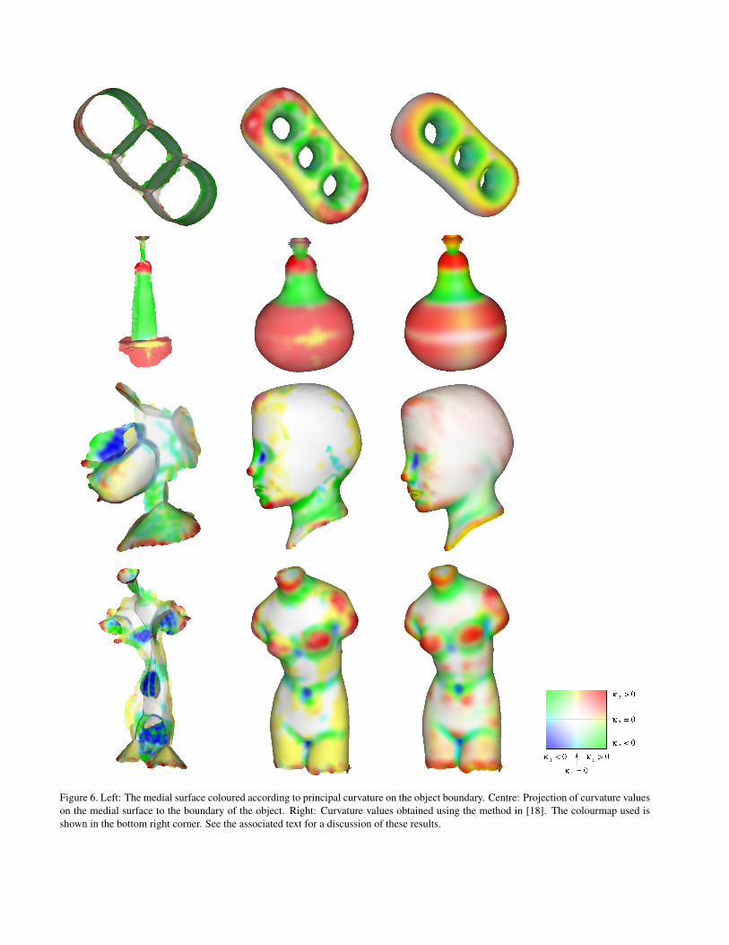
Figure 6. Left: The medial surface coloured according to principal curvature on the object boundary. Centre: Projection of curvature valueson the medial surface to the boundary of the object. Right: Curvature values obtained using the method in [18]. The colourmap used isshown in the bottom right corner. See the associated text for a discussion of these results.

Positive Negative Zeroµ 0.069834 -0.087302 1.205× 10−6

σ 0.000101 0.000148 8.707× 10−6

µ 0.068380 -0.087144 −8.973× 10−7

σ 0.003784 0.002784 1.428× 10−5

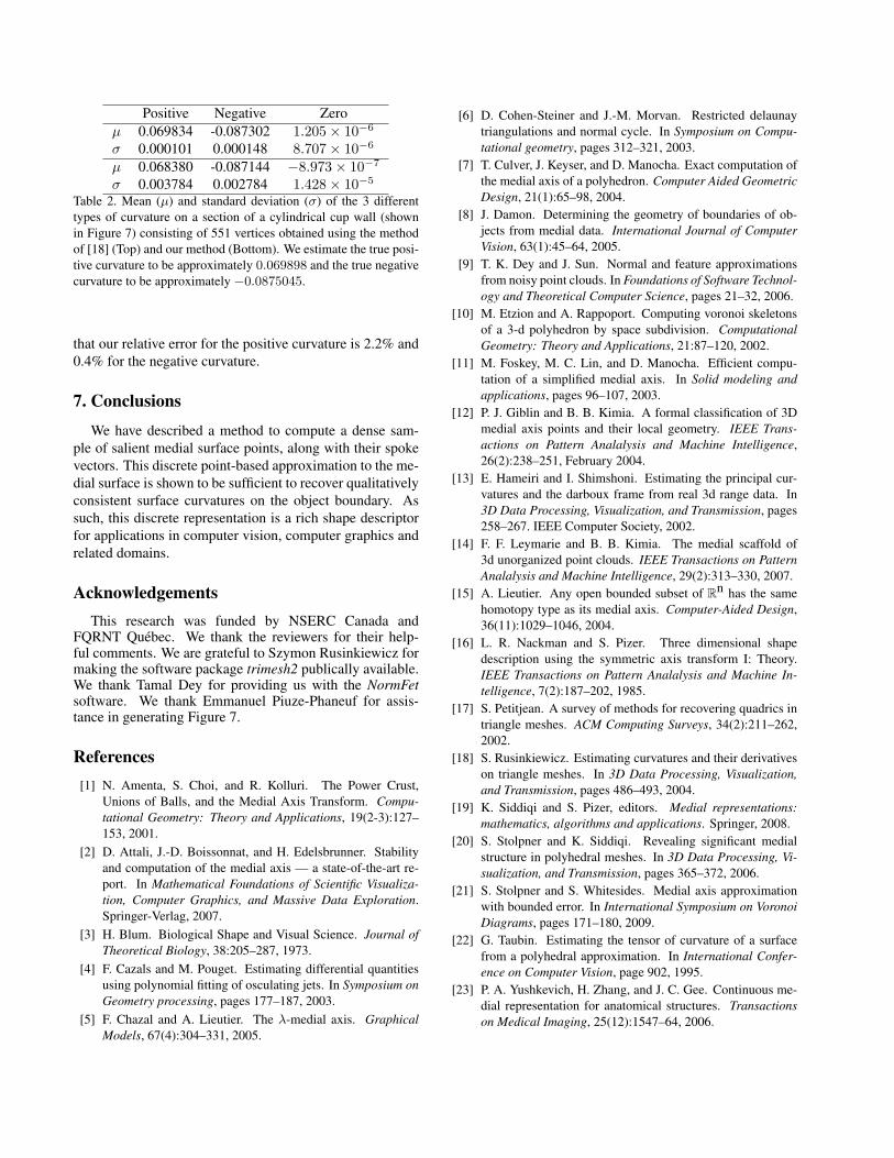
Table 2. Mean (µ) and standard deviation (σ) of the 3 differenttypes of curvature on a section of a cylindrical cup wall (shownin Figure 7) consisting of 551 vertices obtained using the methodof [18] (Top) and our method (Bottom). We estimate the true posi-tive curvature to be approximately 0.069898 and the true negativecurvature to be approximately −0.0875045.

that our relative error for the positive curvature is 2.2% and0.4% for the negative curvature.

7. Conclusions

We have described a method to compute a dense sam-ple of salient medial surface points, along with their spokevectors. This discrete point-based approximation to the me-dial surface is shown to be sufficient to recover qualitativelyconsistent surface curvatures on the object boundary. Assuch, this discrete representation is a rich shape descriptorfor applications in computer vision, computer graphics andrelated domains.

AcknowledgementsThis research was funded by NSERC Canada and

FQRNT Quebec. We thank the reviewers for their help-ful comments. We are grateful to Szymon Rusinkiewicz formaking the software package trimesh2 publically available.We thank Tamal Dey for providing us with the NormFetsoftware. We thank Emmanuel Piuze-Phaneuf for assis-tance in generating Figure 7.

References[1] N. Amenta, S. Choi, and R. Kolluri. The Power Crust,

Unions of Balls, and the Medial Axis Transform. Compu-tational Geometry: Theory and Applications, 19(2-3):127–153, 2001.

[2] D. Attali, J.-D. Boissonnat, and H. Edelsbrunner. Stabilityand computation of the medial axis — a state-of-the-art re-port. In Mathematical Foundations of Scientific Visualiza-tion, Computer Graphics, and Massive Data Exploration.Springer-Verlag, 2007.

[3] H. Blum. Biological Shape and Visual Science. Journal ofTheoretical Biology, 38:205–287, 1973.

[4] F. Cazals and M. Pouget. Estimating differential quantitiesusing polynomial fitting of osculating jets. In Symposium onGeometry processing, pages 177–187, 2003.

[5] F. Chazal and A. Lieutier. The λ-medial axis. GraphicalModels, 67(4):304–331, 2005.

[6] D. Cohen-Steiner and J.-M. Morvan. Restricted delaunaytriangulations and normal cycle. In Symposium on Compu-tational geometry, pages 312–321, 2003.

[7] T. Culver, J. Keyser, and D. Manocha. Exact computation ofthe medial axis of a polyhedron. Computer Aided GeometricDesign, 21(1):65–98, 2004.

[8] J. Damon. Determining the geometry of boundaries of ob-jects from medial data. International Journal of ComputerVision, 63(1):45–64, 2005.

[9] T. K. Dey and J. Sun. Normal and feature approximationsfrom noisy point clouds. In Foundations of Software Technol-ogy and Theoretical Computer Science, pages 21–32, 2006.

[10] M. Etzion and A. Rappoport. Computing voronoi skeletonsof a 3-d polyhedron by space subdivision. ComputationalGeometry: Theory and Applications, 21:87–120, 2002.

[11] M. Foskey, M. C. Lin, and D. Manocha. Efficient compu-tation of a simplified medial axis. In Solid modeling andapplications, pages 96–107, 2003.

[12] P. J. Giblin and B. B. Kimia. A formal classification of 3Dmedial axis points and their local geometry. IEEE Trans-actions on Pattern Analalysis and Machine Intelligence,26(2):238–251, February 2004.

[13] E. Hameiri and I. Shimshoni. Estimating the principal cur-vatures and the darboux frame from real 3d range data. In3D Data Processing, Visualization, and Transmission, pages258–267. IEEE Computer Society, 2002.

[14] F. F. Leymarie and B. B. Kimia. The medial scaffold of3d unorganized point clouds. IEEE Transactions on PatternAnalalysis and Machine Intelligence, 29(2):313–330, 2007.

[15] A. Lieutier. Any open bounded subset of Rn has the samehomotopy type as its medial axis. Computer-Aided Design,36(11):1029–1046, 2004.

[16] L. R. Nackman and S. Pizer. Three dimensional shapedescription using the symmetric axis transform I: Theory.IEEE Transactions on Pattern Analalysis and Machine In-telligence, 7(2):187–202, 1985.

[17] S. Petitjean. A survey of methods for recovering quadrics intriangle meshes. ACM Computing Surveys, 34(2):211–262,2002.

[18] S. Rusinkiewicz. Estimating curvatures and their derivativeson triangle meshes. In 3D Data Processing, Visualization,and Transmission, pages 486–493, 2004.

[19] K. Siddiqi and S. Pizer, editors. Medial representations:mathematics, algorithms and applications. Springer, 2008.

[20] S. Stolpner and K. Siddiqi. Revealing significant medialstructure in polyhedral meshes. In 3D Data Processing, Vi-sualization, and Transmission, pages 365–372, 2006.

[21] S. Stolpner and S. Whitesides. Medial axis approximationwith bounded error. In International Symposium on VoronoiDiagrams, pages 171–180, 2009.

[22] G. Taubin. Estimating the tensor of curvature of a surfacefrom a polyhedral approximation. In International Confer-ence on Computer Vision, page 902, 1995.

[23] P. A. Yushkevich, H. Zhang, and J. C. Gee. Continuous me-dial representation for anatomical structures. Transactionson Medical Imaging, 25(12):1547–64, 2006.