Sample Problem Set – SOLUTIONSinside.mines.edu/~whoff/courses/EENG510/lectures/samplesolns.pdf · 1 . Sample Problem Set – SOLUTIONS . The exam covers these sections in the Gonzalez

CSCI 510 / EENG 510

1

Sample Problem Set – SOLUTIONS The exam covers these sections in the Gonzalez and Woods textbook: Ch 2, 3.1-3.6, 4.1-4.10, 9.1-9.3, 10.1-10.2.6. It will be closed book, but handwritten notes are allowed. The problems below are representative of exam problems (although there may be more problems than would appear on the actual exam). Some of the problems below are drawn from previous exams. For reference, here are some important properties and equations (this will be provided):

Fourier transform

1 12 ( / / )

0 0( , ) ( , )

M Nj ux M vy N

x yF u v f x y e π

− −− +

= =

= ∑∑ (discrete)

2 ( )( , ) ( , ) j ux vyF u v f x y e dx dyπ∞ ∞ − +

−∞ −∞= ∫ ∫ (continuous)

Inverse Fourier transform

1 12 ( / / )

0 0

1( , ) ( , )M N

j ux M vy N

u vf x y F u v e

MNπ

− −+

= =

= ∑∑ (discrete)

2 ( )( , ) ( , ) j ux vyf x y F u v e du dvπ∞ ∞ +

−∞ −∞= ∫ ∫ (continuous)

Important Fourier pairs )(

)(22/)(2

)()sin(

)()sin(],[)(

21)(

1),()(2222222

vbuaj

vuyx

evb

vbua

uaabbarectfunctrect

eeGaussian

yximpulse

+−

+−+−

⇔

⇔

⇔

π

σπσ

ππ

ππ

πσ

δ

Convolution ∑∑−

=

−

=

−−=∗1

0

1

0),(),(),(),(

M

m

N

nnymxhnmfyxhyxf

Correlation 1 1

*

0 0( , ) ( , ) ( , ) ( , )

M N

m nf x y h x y f m n h x m y n

− −

= =

⊗ = + +∑∑

Translation )//(200

)//(200

00

00

),(),(

),(),(NyvMxuj

NvyMuxj

eyxfvvuuF

evuFyyxxf+

+−

⇔−−

⇔−−π

π

Scaling )/,/(1),(

),(),(

bvauFab

byaxf

vuaFyxaf

⇔

⇔

Rotation ),(),(

coscossincos

00 θφωθθφφθθ

+⇔+====

Frfrwruryrx

Morphological erosion ( ){ }θz

A B z B A= ⊆ or ( ){ }θ cz

A B z B A= ≠ ∅

Morphological dilation ( ){ }ˆz

A B z B A⊕ = ≠ ∅

CSCI 510 / EENG 510

2

1. The image of stripes below on the left is too dark when displayed on a monitor. To improve the display, we apply a gamma transformation to produce the image on the right.

Sketch the gray level transformation for a gamma transformation that will produce the image on the right. Solution:

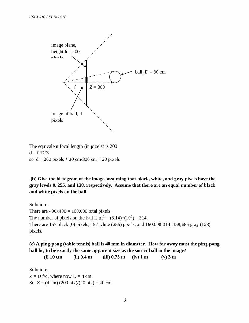
with s crγ= and 1γ < 2. A digital camera captures a 400x400 pixel image of a black and white soccer ball on a

gray background. The ball is 30 cm in diameter and is 3 m away from the camera. The camera has a field of field of 90 degrees horizontally and vertically.

(a) What is the diameter of the ball in pixels, in the image? (i) 3 pixels (ii) 10 pixels (iii) 20 pixels (iv) 31 pixels (v) 63 pixels Solution: D/Z = d/f

Gray level in

Gra

y le

vel o

ut

CSCI 510 / EENG 510

3

The equivalent focal length (in pixels) is 200. d = f*D/Z so d = 200 pixels * 30 cm/300 cm = 20 pixels (b) Give the histogram of the image, assuming that black, white, and gray pixels have the gray levels 0, 255, and 128, respectively. Assume that there are an equal number of black and white pixels on the ball. Solution: There are 400x400 = 160,000 total pixels. The number of pixels on the ball is πr2 = (3.14)*(102) = 314. There are 157 black (0) pixels, 157 white (255) pixels, and 160,000-314=159,686 gray (128) pixels. (c) A ping-pong (table tennis) ball is 40 mm in diameter. How far away must the ping-pong ball be, to be exactly the same apparent size as the soccer ball in the image? (i) 10 cm (ii) 0.4 m (iii) 0.75 m (iv) 1 m (v) 3 m Solution: Z = D f/d, where now D = 4 cm So Z = (4 cm) (200 pix)/(20 pix) = 40 cm

image plane, height h = 400 pixels

Z = 300

ball, D = 30 cm

image of ball, d pixels

f

CSCI 510 / EENG 510

4

3. A CCD camera has a image resolution of 2000 x 2000 pixels. The individual sensor

elements are squares measuring 10 x 10 um, with no spaces between them. a. If the camera uses a lens with focal length = 100 mm, what is the field of view? b. Assume the camera is mounted on an airplane, pointing straight down at the

ground. What height should the airplane fly, so that one pixel in the camera corresponds to one meter on the ground?

Solution: (a) The size of the image plane is 2000x10 um square. This is (2 x 10^3)(10 x 10^-6 m) = 20 x 10^-3 = 20 mm. The field of view is 2 atan(10 mm/100 mm) = 2 atan(0.1) = 2 (5.7) = 11.4 degrees. (b) If one pixel is one meter, then the entire image covers 2000x2000 meters. f/w = H/W (100 mm)/(20 mm) = H/(2000 m) or H = 10000 m

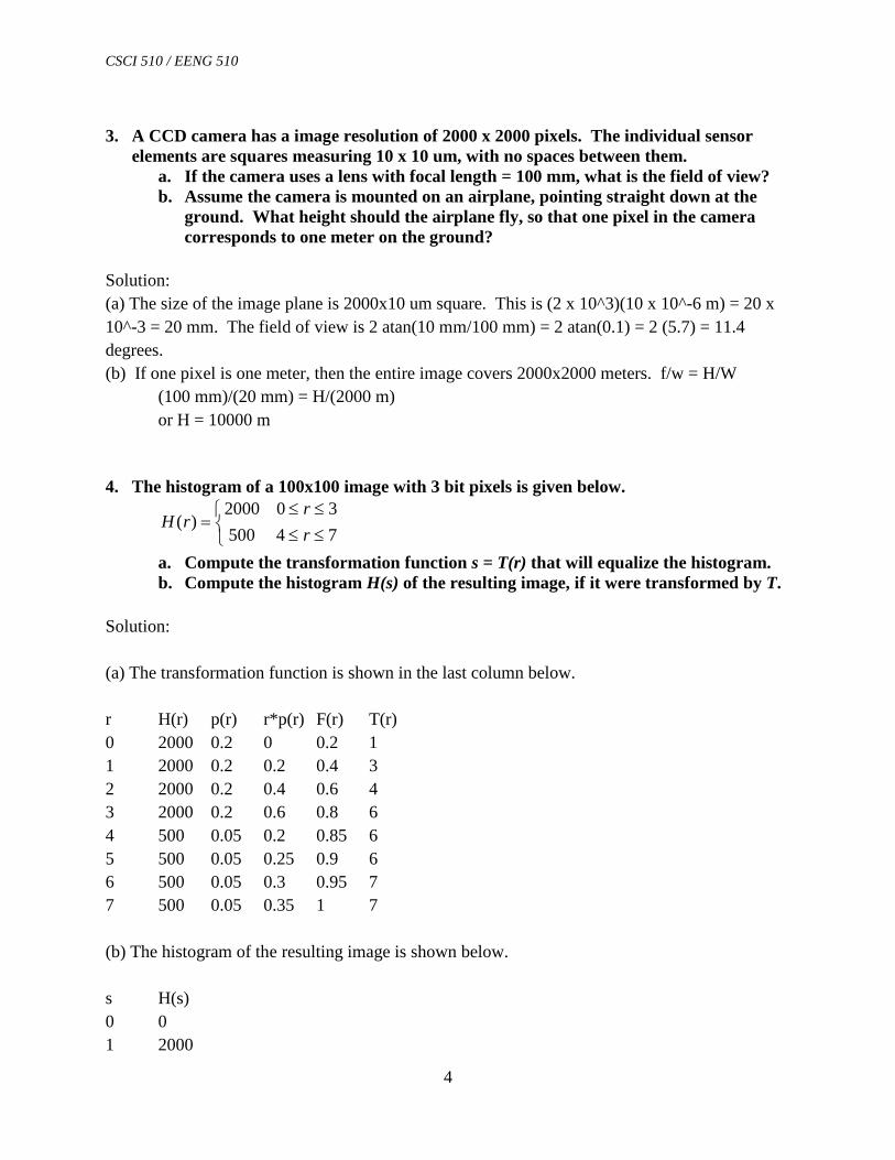
4. The histogram of a 100x100 image with 3 bit pixels is given below.

≤≤≤≤

=74500302000

)(rr

rH

a. Compute the transformation function s = T(r) that will equalize the histogram. b. Compute the histogram H(s) of the resulting image, if it were transformed by T.

Solution: (a) The transformation function is shown in the last column below. r H(r) p(r) r*p(r) F(r) T(r) 0 2000 0.2 0 0.2 1 1 2000 0.2 0.2 0.4 3 2 2000 0.2 0.4 0.6 4 3 2000 0.2 0.6 0.8 6 4 500 0.05 0.2 0.85 6 5 500 0.05 0.25 0.9 6 6 500 0.05 0.3 0.95 7 7 500 0.05 0.35 1 7 (b) The histogram of the resulting image is shown below. s H(s) 0 0 1 2000

CSCI 510 / EENG 510

5

2 0 3 2000 4 2000 5 0 6 3000 7 1000 5. Complete the following Matlab code to do a correlation between a 10x10 template

image T and a 100x100 image I (you do not have to normalize the result). % Assume that I, T are already loaded corr = zeros(100); % resulting correlation image for r=1:90 for c=1:90 % Compute the score for this point (r,c) : (your code goes here) corr(r,c) = score; end end

Solution: corr = zeros(100); % resulting correlation image for r=1:90 for c=1:90 score = 0; for m=1:10 for n=1:10 score = score + I(r+m, c+n) * T(m,n); end end corr(r,c) = score; end end

Note that the above assumes that the origin of the template is at the top left corner; i.e., T(1,1). If the origin of the template is in the middle you could do corr = zeros(100); % resulting correlation image for r=5:95 for c=5:95 score = 0; for m=-4:5

CSCI 510 / EENG 510

6

for n=-4:5 score = score + I(r+m, c+n) * T(m+5,n+5); end end corr(r,c) = score; end end

6. Compute the convolution of the following image with the filter w (assume that the

origin of w is at its center). To compute the result at the border, pad the image with zeros.

1 1 1

0 0 01 1 1

w− − − =

Image: 0 0 0 0 0 0 0 0

0 0 0 0 0 0 0 0

0 0 10 10 10 10 0 0

0 0 10 10 10 10 0 0

0 0 10 10 10 10 0 0

0 0 10 10 10 10 0 0

0 0 0 0 0 0 0 0

0 0 0 0 0 0 0 0 Result:

CSCI 510 / EENG 510

7

Solution: For convolution we have to rotate w by 180° and then do the sum of products at each position. 0 0 0 0 0 0 0 0

0 -10

-20

-30

-30

-20

-10

0

0 -10

-20

-30

-30

-20

-10

0

0 0 0 0 0 0 0 0

0 0 0 0 0 0 0 0

0 10 20 30 30 20 10 0

0 10 20 30 30 20 10 0

0 0 0 0 0 0 0 0 7. Consider a 3x3 spatial mask that averages the four closest neighbors of a point (x,y) but

excludes the point itself from the average. Find the equivalent filter, H(u,v) in the frequency domain. (Hint: Use the translation property of the Fourier transform).

Solution: We have g(x,y) = [ f(x+1,y) + f(x-1,y) + f(x,y+1) + f(x,y-1)]/4. By linearity,

{ } { } { } { }1( , ) ( 1, ) ( 1, ) ( , 1) ( , 1)4

G u v f x y f x y f x y f x y = + + − + + + − F F F F . By the translation

property, 2 / 2 / 2 / 2 /1( , ) ( , ) ( , ) ( , ) ( , )4

j u M j u M j v N j v NG u v F u v e F u v e F u v e F u v eπ π π π− − = + + + . So the

equivalent filter is 2 / 2 / 2 / 2 /1( , )4

j u M j u M j v N j v NH u v e e e eπ π π π− − = + + + .

You can see that this acts like a low pass filter. At (u,v)=(0,0), H(u,v)=1. The values of H(u,v) decrease as (u,v) move away from the origin. Although you wouldn’t need to implement Matlab code on an exam, we can plot the magnitude of H:

CSCI 510 / EENG 510

8

At very high frequencies (where both u and v are high), the magnitude of H starts to rise again, so it does not attenuate those high frequencies like a low pass filter should. The Matlab code for this: M = 100; N = 100; [u,v] = meshgrid(-M/2:M/2, -N/2:N/2); H = (1/4)*( exp(j*2*pi*u/M) + exp(-j*2*pi*u/M) + ... exp(j*2*pi*v/N) + exp(-j*2*pi*v/N) ); Habs = abs(H); figure, imshow(Habs, []), impixelinfo figure, surf(Habs), colormap jet; What would H(u,v) look like for a 3x3 box averaging filter?

8. You want to apply the Laplacian of a Gaussian edge operator, G2∇ to an image f(x, y) of size 512x512. Assume that the edge operator is of size 32x32, and that its origin is at its center. Describe in words how to perform this in the frequency domain.

Solution: 1. Create the 32x32 edge operator in the spatial domain, and zero pad it to size 512x512.

0 2040 60 80

100

0

50

100

1500

0.2

0.4

0.6

0.8

1

CSCI 510 / EENG 510

9

2. Compute the 2D Fourier transforms of zero-padded image and mask. 3. Take the product of the Fourier transforms. 4. Take the inverse Fourier transform of the result. Take the real part of that (it should be real anyway). 5. Shift the resulting image by (-16, -16). This is because doing the convolution this way assumes that the origin of the operator is at its upper left corner, instead of the middle. 9. Describe the Fourier transform of a filter that performs smoothing with the ideal low

pass filter, followed by differentiation in the x direction. Sketch a plot of its magnitude. Notes: The Fourier transform of the ideal low pass filter is:

( )

>+≤+

= 222

222

01

,RvuRvu

vuH

The Fourier transform equivalent of differentiation is

( ) ( ) ( ),2 ,

nn

n

f x yj u F u v

xπ

∂⇔

∂

Smoothing followed by differentiation is

( ) fhx

fhx

∗

∗∂∂

=∗∗

∂∂

Solution: Convolution in the spatial domain is equivalent to multiplication in the frequency domain. The resulting filter is

( )2 2 2

2 2 2

2,

0j u u v R

H u vu v R

π + ≤=

+ >

Here is the x-derivative filter and the ideal low pass filter:

CSCI 510 / EENG 510

10

Here is the combined filter, obtained by point by point multiplication (zoomed in). Also show in 3D.

Here is “moon” image, and the results of applying the combined filter:

CSCI 510 / EENG 510

11

The Matlab source file: % Get a sample image I=imread('moon.tif'); imshow(I,[]); sizeI=size(I); u0 = sizeI(2)/2; v0 = sizeI(1)/2; FI=fft2(I); % Construct the x-derivative operator for u=1:sizeI(2) for v=1:sizeI(1) FE(v,u) = (u-u0)*i*2*pi; end end figure,imshow(abs(FE),[]); % Apply the x-derivative to the image FG = FI .* fftshift(FE); G=ifft2(FG); figure, imshow(abs(G),[]); % Construct ideal low pass filter R2 = 20^2; for u=1:sizeI(2) for v=1:sizeI(1) if (u-u0)^2 + (v-v0)^2 < R2

CSCI 510 / EENG 510

12

FLP(v,u) = 1; else FLP(v,u) = 0; end end end figure, imshow(abs(FLP),[]); % Apply ideal low pass filter to the image FH = fftshift(FLP) .* FI; H = ifft2(FH); figure, imshow(abs(H),[]); % Now apply a combined operator to the image FK = FE .* FLP; figure, imshow(abs(FK),[]); FL=FI .* fftshift(FK); L=ifft2(FL); figure, imshow(abs(L),[]);

10. Assume that the 2D Fourier transform of the MxN image f(x,y) is F(u,v). Determine

the 2D Fourier transform of the following functions. You may wish to refer to the properties of the Fourier transform in the table on the front page.

a. 4 f(2x - 4, y + 2)

(select one) (i) 2 (2 / 2 / )2 ( / 2, )j u M v Ne F u vπ− −

(ii) 2 (2 / / )4 ( / 2, )j u M v Ne F u vπ− −

(iii) 2 (4 / 2 / )2 ( / 2, / 2)j u M v Ne F u vπ− −

(iv) )2/,(4 )/2/(2 vuFe NvMuj −− π Solution: This function involves both translation and scaling. First define a function f1(x,y):

)2,4(),(1 +−= yxfyxf Its Fourier transform is ),(),( )/2/4(2

1 vuFevuF NvMuj −−= π Now define

2 1( , ) 4 (2 , ) 4 (2 4, 2)f x y f x y f x y= = − + 1 Its Fourier transform is

),2/(2),2/(214),( )/2/2(2

12 vuFevuFvuF NvMuj −−=⋅= π

1 This step may be a little tricky to follow. Let’s take a simpler example: f(x) = x^2. Define f1(x) = f(x-4)=(x-4)^2. Then define f2(x) = f1(2x). You substitute 2x in place of x in the expression for f1, to get f2(x)=(2x-4)^2.

CSCI 510 / EENG 510

13

Or, you could do the scaling first and then the translation. Define function f1(x,y): 1( , ) 4 (2 , )f x y f x y=

Its Fourier transform is 1( , ) 2 ( / 2, )F u v F u v= Now define

( )( )2 1( , ) ( 2, 2) 2 2 2 , 2f x y f x y f x y= − + = − + Its Fourier transform is 2 (2 / 2 / ) 2 (2 / 2 / )

2 1( , ) ( , ) 2 ( / 2, )j u M v N j u M v NF u v F u v e F u v eπ π− − − −= =

b. f(x - 3, y + 2) * f(x + 3, y) (where * denotes convolution)

(select one) (i) 2 ( / ) ( , )j v Ne F u vπ

(ii) 2 ( , )F u v

(iii) 2 ( / 2 / ) 2 ( , )j u M v Ne F u vπ −

(iv) 2 (2 / ) 2 ( , )j v Ne F u vπ

Solution:

),(),3(

),()2,3()/3(2

)/2/3(2

vuFeyxfvuFeyxf

Muj

NvMuj

π

π

⇔+

⇔+− −−

Thus

),(),(),(),3()2,3(

2)/2(2

)/3(2)/2/3(2

vuFevuFvuFeeyxfyxf

Nvj

MujNvMuj

π

ππ

=

⇔+∗+− −−

. 11. The following is a binary image I and a structuring element S. Assume that the origin

of S lies at its center.

CSCI 510 / EENG 510

14

I: S: 0 1 2 3 4 5 6 7 8 9 0 1 2 1 1 1 1 1 1 3 1 1 1 1 4 1 1 1 1 1 5 1 1 1 1 1 1 6 1 1 1 1 1 1 7 1 1 1 1 1 1 8 9

(a) Predict the result of dilating I with S.

0 1 2 3 4 5 6 7 8 9 0 1 1 1 1 1 1 1 2 1 1 1 1 1 1 1 1 3 1 1 1 1 1 1 1 4 1 1 1 1 1 1 1 1 5 1 1 1 1 1 1 1 1 6 1 1 1 1 1 1 1 1 7 1 1 1 1 1 1 1 1 8 1 1 1 1 1 1 9

(b) Predict the result of eroding I with S.

1 1 1 1 1

CSCI 510 / EENG 510

15

0 1 2 3 4 5 6 7 8 9 0 1 2 3 1 4 1 5 1 1 1 6 1 1 1 1 7 8 9

12. A small portion of a binary image I is shown below. Assume that you want to join the two groups of 1’s into a single connected group, while distorting the overall image as little as possible (this might be from an image of a fingerprint, for example).

a. Using the structuring element S shown below, would you use morphological opening or morphological closing?

b. Apply the operation you selected in (a) to the image I. (Assume that there are 0’s outside the border of the image.) Show the intermediate results of dilation and erosion (or vice versa).

I: 1 1 1 1 1 1 1 1 1 1 1 1 1 1 1

S (the origin of S is in the upper left):

1 1 1 1

Solution: We would do a morphological closing, which is a dilation followed by an erosion.

CSCI 510 / EENG 510

16

The dilation of I by S is shown below. It consists of all the original 1’s, plus some new 1’s. Bold (and red) indicate the new 1’s.

1 1 1 1 1 1 1 1 1 1 1 1 1 1 1 1 1 1 1 1 1 1 1 1 1 1 1

The erosion of the above by S is shown below. It is the same as the original except that there is an additional “1” joining the two groups, and we have lost the 1’s on the rightmost column because of the assumption that there were 0’s beyond the border.

1 1 1 1 1 1 1 1 1 1 1 1 1 1

13. A camera takes images of a test pattern. The image is converted to binary, as shown in

the left image. Occasionally, diagonal streaks appear in the image due to some unknown noise process, as shown in the right image. To help diagnose the problem, we want to create an algorithm that will automatically count the streaks. It is observed that the streaks are always at the same angle (45 degrees), between 35 and 50 pixels long, and between 2 and 4 pixels wide. Describe an algorithm, based on morphological processing, that will automatically count the streaks. (Be as specific as possible!)

CSCI 510 / EENG 510

17

Solution: We assume that there are no structures in the image (other than the noise stripes) that are longer than 35 pixels. We create a structuring element that is a line at 45 degrees, 35 pixels long, and 2 pixels wide (ie, the minimum size). We “open” the image with this structuring element (“imopen” in Matlab), and then use a connected component labeling algorithm (“bwlabel” in Matlab) to count the objects. An opened image is shown below. Actually, if all you want to do is to count the streaks (instead of producing an image of the streaks), you can simply erode the original image with the line structuring element, and count the number of connected components. Finally, note the extra blob on the right hand side of the image. This is due to the fact that when you erode, the image is effectively padded with 1’s outside the boundary. So the line actually fits partially inside the white area at the right edge, with the remainder falling outside in the 1’s.

CSCI 510 / EENG 510

18

14. Explain why the edges found by the Laplacian of a Gaussian edge operator form closed

contours. Solution: The edges are the zero crossings of the values resulting from convolving the image with the Laplacian of Gaussian operator. In other words, the edges are the boundary between regions with negative values and regions with positive values. Those regions are connected components. A contour surrounding a connected component must be a closed path.