10 100 1,000 Resistivity ohm-m From induction tool 16-in. normal 0 20 40 60 80 100 Depth in meters 100 200 Gamma cps 500 1,000 1,500 Neutron cps SP -50 0 mV 0 50 150 200 250 300 Depth in feet 100 ? 50 150 200 250 300 100 Depth in feet 0 Elevation 7,549 ft (2,301 m) Electrical conductor Prepared in cooperation with National Park Service Sample Descriptions and Geophysical Logs for Cored Well BP-3-USGS, Great Sand Dunes National Park, Alamosa County, Colorado Data Series 918 U.S. Department of the Interior U.S. Geological Survey

Welcome message from author
This document is posted to help you gain knowledge. Please leave a comment to let me know what you think about it! Share it to your friends and learn new things together.
Transcript

10 100 1,000
Resistivity
ohm-m
From inductiontool
16-in.normal
0
20
40
60
80
100
Dept
h in
met
ers
100 200
Gamma
cps500 1,000 1,500
Neutron
cps
SP
-50 0mV
0
50
150
200
250
300
Dept
h in
feet
100
?
50
150
200
250
300
100De
pth
in fe
et
0Elevation
7,549 ft(2,301 m)
Electricalconductor
Prepared in cooperation with National Park Service
Sample Descriptions and Geophysical Logs for Cored Well BP-3-USGS, Great Sand Dunes National Park, Alamosa County, Colorado
Data Series 918
U.S. Department of the InteriorU.S. Geological Survey

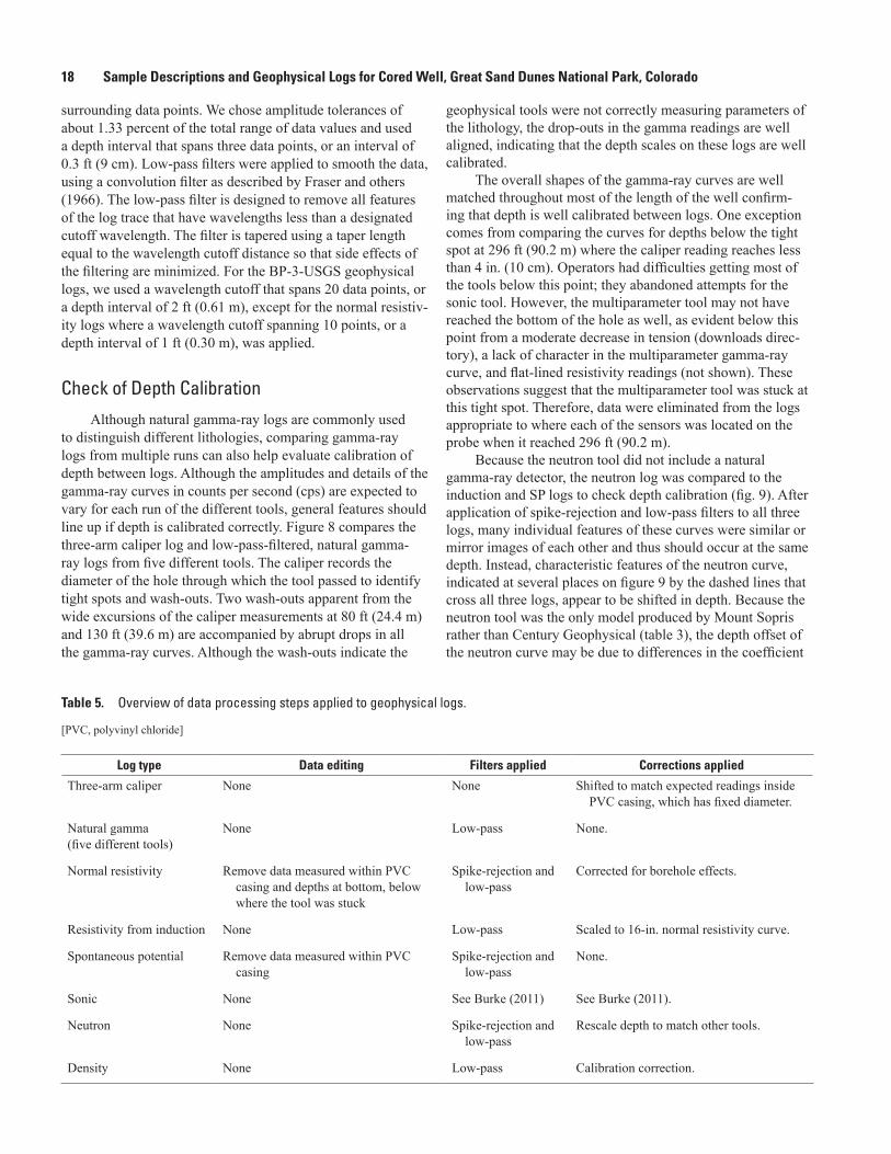
Cover. Selected generalized geophysical logs and generalized lithologic logs for BP-3-USGS. Photographs from top to bottom: At the end of a core run, the barrel is lifted out of the hole onto one of the several sawhorse setups. Clay from the same sample as in A after almost 5 years of storage in a plastic bag. Stream of water that was flowing out of the drill stem into the mud pool the morning of September 17, 2009. Clay with blue tint at time of collection as a core catcher sample at 266 ft depth (core run 19). B, Clay with even-gray color at time of collection from ≈311 ft depth (core run 26). Intact core after extrusion onto a split half of polyvinyl chloride pipe on a sawhorse apparatus.

Sample Descriptions and Geophysical Logs for Cored Well BP-3-USGS, Great Sand Dunes National Park, Alamosa County, Colorado
By V.J.S. Grauch, Gary L. Skipp, Jonathan V. Thomas, Joshua K. Davis, and Mary Ellen Benson
Prepared in cooperation with National Park Service
Data Series 918
U.S. Department of the InteriorU.S. Geological Survey

U.S. Department of the InteriorSALLY JEWELL, Secretary
U.S. Geological SurveySuzette M. Kimball, Acting Director
U.S. Geological Survey, Reston, Virginia: 2015
For more information on the USGS—the Federal source for science about the Earth, its natural and living resources, natural hazards, and the environment—visit http://www.usgs.gov or call 1–888–ASK–USGS.
For an overview of USGS information products, including maps, imagery, and publications, visit http://www.usgs.gov/pubprod/.
Any use of trade, firm, or product names is for descriptive purposes only and does not imply endorsement by the U.S. Government.
Although this information product, for the most part, is in the public domain, it also may contain copyrighted materials as noted in the text. Permission to reproduce copyrighted items must be secured from the copyright owner.
Suggested citation:Grauch, V.J.S., Skipp, G.L., Thomas, J.V., Davis, J.K., and Benson, M.E., 2015, Sample descriptions and geophysical logs for cored well BP-3-USGS, Great Sand Dunes National Park and Preserve, Alamosa County, Colorado: U.S. Geological Survey Data Series 918, 53 p., http://dx.doi.org/10.3133/ds918.
ISSN 2327-638X (online)
iii
Contents
Abstract ...........................................................................................................................................................1Introduction.....................................................................................................................................................1Regional Setting and Geophysical Studies ...............................................................................................3Drilling Operations .........................................................................................................................................4Procedures for Lithologic Descriptions .....................................................................................................6
Sampling Procedures ...........................................................................................................................6Mud Stream Samples ..................................................................................................................6Core Barrel Samples ...................................................................................................................6
Effects of Storage and Handling ......................................................................................................10Laboratory Methods ...........................................................................................................................13Sample Descriptions Versus Well Depths ......................................................................................13
Geophysical Logs .........................................................................................................................................16Logs Acquired......................................................................................................................................16Data Processing ..................................................................................................................................16
Check of Depth Calibration ......................................................................................................18Normal Resistivity Logs ............................................................................................................21Induction Log ..............................................................................................................................21Density and Sonic Logs ............................................................................................................21
Digital Log Files ...................................................................................................................................26Summary of Findings ...................................................................................................................................26Significance for Future Studies .................................................................................................................28Acknowledgments .......................................................................................................................................30References Cited..........................................................................................................................................30
Figures 1. Map showing location of BP-3-USGS well, the inferred limit of the last high stand of
Pliocene and Pleistocene Lake Alamosa before its disappearance and the Hansen Bluff core site near Great Sand Dunes National Park and Preserve in Alamosa County of southern Colorado ......................................................................................................3
2. Photographs of drilling operations ............................................................................................5 3. Photographs of various sampling procedures for mud stream samples ............................8 4. Photographs of various sampling procedures for core barrel samples .............................9 5. Photographs of a selected core at time of collection compared to more than
4 years later .................................................................................................................................11 6. Photographs of two clay samples of differing color at time of collection in
September 2009 compared to almost 5 years later in August 2014 ....................................12 7. Graphical summary of lithologic descriptions and other observations versus
inferred well depth .....................................................................................................................14 8. Diagram showing borehole diameter measured by the three-arm caliper and
low-pass-filtered, natural gamma-ray curves from five different tools ............................19 9. Diagram showing comparison of original neutron curve to induction and
spontaneous potential logs to correct the depth scale for the neutron log .....................20

iv
10. Diagram showing normal resistivity curves from the multiparameter tool before and after data processing .................................................................................................................22
11. Diagram showing resistivity derived from the induction tool before and after data processing compared to normal resistivity curves after data processing .......................23
12. Diagram showing resistivity curves after data processing compared to resistivity layers derived from a time-domain electromagnetic sounding measured at the site before drilling ..............................................................................................................................24
13. Diagram showing sonic velocity and compensated density logs ......................................25 14. Diagram showing selected geophysical logs and generalized lithologic log for
BP-3-USGS ...................................................................................................................................27
Tables 1. Explanation of and procedures for different sample types ...................................................7 2. Core lengths recovered onsite in 2009 and changes in measured lengths in years
2012 and 2013 ...............................................................................................................................10 3. Geophysical tools and associated data logs acquired for BP-3-USGS, listed in the
order they were acquired ..........................................................................................................16 4. Description of geophysical logs and their utility for BP-3-USGS .......................................17 5. Overview of data processing steps applied to geophysical logs .......................................18
Appendix Tables 1. Descriptions of samples by type and drilling interval...........................................................34 2. Depth intervals where fossils or other evidence of life were observed ...........................47 3. Results of analysis by X-ray powder diffraction ...................................................................53
Download FilesLog files—data for borehole geophysical logs
http://pubs.usgs.gov/ds/0918/downloads/LogFiles/
Photographs of samples taken onsite http://pubs.usgs.gov/ds/0918/downloads/PhotoFiles/

v
Conversion FactorsInch/Pound to SI
Multiply By To obtain
Length
inch (in.) 2.54 centimeter (cm)inch (in.) 25.4 millimeter (mm)foot (ft) 0.3048 meter (m)mile (mi) 1.60934 kilometer (km)
Density
grams per cubic centimeter (g/cm3) 1,000.0 kilograms per cubic meter (kg/m3)Velocity
foot per second (ft/s) 0.3048 meter per second (m/s)Flow rate
gallon per minute (gal/min) 0.06309 liter per second (L/s)Electrical resistivity
ohm-meters (ohm-m) 0.001 kiloohm-meters (kohm-m)Electrical conductivity
millimhos per meter (mmhos/m) 1,000.0 siemens per meter (S/m)Electrical potential
millivolts (mV) 1,000.0 volts (V)
Supplemental InformationElectrical resistivity ρ in ohm-meters (ohm-m) can be converted to electrical conductivity σ in siemens per meter (S/m) as follows: σ = 1/ρ.
DatumsVertical coordinate information is referenced to the North American Vertical Datum of 1988 (NAVD 88).
Horizontal coordinate information is referenced to the North American Datum of 1983 (NAD 83).
Elevation, as used in this report, refers to distance above the vertical datum.

vi
Abbreviations Used in This Report
cps counts per second
EM electromagnetic
ka kilo-annum (thousand years)
Ma Mega-annum (million years)
NPS National Park Service
PVC polyvinyl chloride
TEM time-domain electromagnetic
USGS U.S. Geological Survey
Introduction 1
Sample Descriptions and Geophysical Logs for Cored Well BP-3-USGS, Great Sand Dunes National Park, Alamosa County, Colorado
By V.J.S. Grauch,1 Gary L. Skipp,1 Jonathan V. Thomas,1 Joshua K. Davis,2 and Mary Ellen Benson1
1U.S. Geological Survey.
2University of Texas at Austin.
AbstractThe BP-3-USGS well was drilled at the southwestern
corner of Great Sand Dunes National Park in the San Luis Valley, south-central Colorado, 68 feet (ft, 20.7 meters [m]) southwest of the National Park Service’s boundary-piezometer (BP) well 3. BP-3-USGS is located at latitude 37°43ʹ18.06ʺN. and longitude 105°43ʹ39.30ʺW., at an elevation of 7,549 ft (2,301 m). The well was drilled through poorly consoli-dated sediments to a depth of 326 ft (99.4 m) in September 2009. Water began flowing from the well after penetrating a clay-rich layer that was first intercepted at a depth of 119 ft (36.3 m). The base of this layer, at an elevation of 7,415 ft (2,260 m) above sea level, likely marks the top of a regional confined aquifer recognized throughout much of the San Luis Valley. Approximately 69 ft (21 m) of core was recovered (about 21 percent), almost exclusively from clay-rich zones. Coarser grained fractions were collected from mud extruded from the core barrel or captured from upwelling drilling fluids. Natural gamma-ray, full waveform sonic, density, neutron, resistivity, spontaneous potential, and induction logs were acquired. The well is now plugged and abandoned.
This report presents lithologic descriptions from the well samples and core, along with a compilation and basic data pro-cessing of the geophysical logs. The succession of sediments in the well can be generalized into three lithologic packages: (1) mostly sand from the surface to about 77 ft (23.5 m) depth; (2) interbedded sand, silt, and clay, decreasing in overall grain size downward, from 77 to 232 ft (23.5 to 70.7 m) depth; and (3) layers of massive clay alternating with layers of fine sand to silt from 232 to 326 ft (70.7 to 99.4 m), the total depth of the well. The topmost clay layers of the deepest package have a blue tint, prompting a correlation with the “blue clay” of the San Luis Valley that is commonly considered as the top of the confined aquifer. However, a confining clay was intercepted 113 ft (34.4 m) higher than the blue clay in BP-3-USGS.
Most of the geophysical logs have good correspondence to the lithologic variations in the well. Exceptions are the gamma-ray log, which is likely affected by naturally occurring radiation from abundant volcanic detritus, and one interval within the deepest lithologic package, which appears to be abnormally electrically conductive. Resistivity logs and varia-tions in sand versus clay content within the well are consistent with electrical resistivity models derived from time-domain electromagnetic geophysical surveys for the area. In particu-lar, the topmost blue clay corresponds to a strong electrical conductor that is prominent in the electromagnetic geophysical data throughout the park and vicinity.
BP-3-USGS was sited to test hypotheses developed from geophysical studies and to answer questions about the his-tory and evolution of Pliocene and Pleistocene Lake Alamosa, which is represented by lacustrine deposits sampled by the well. The findings reported here represent a basis from which future studies can answer these questions and address other important scientific questions in the San Luis Valley regarding geologic history and climate change, groundwater hydrology, and geophysical interpretation.
IntroductionThe U.S. Geological Survey (USGS) has been conduct-
ing geologic and geophysical studies for several years in the San Luis Valley, Colorado, under the auspices of the National Cooperative Geologic Mapping Program. The goals are to improve understanding of the present-day geologic framework in three dimensions and its geologic history. A combination of drill-hole information, geophysical methods, and geo-logic mapping provide the most comprehensive approach to determining the third dimension of geology that underlies the landscape.
One focus of the USGS studies has centered on the evolution and nature of deposits left behind by a large lake that occupied most of the San Luis Valley in the Pliocene and Pleistocene (Siebenthal, 1910). Recent geologic investiga-tions conclude that this ancient Lake Alamosa formed about
2 Sample Descriptions and Geophysical Logs for Cored Well, Great Sand Dunes National Park, Colorado
3 million years ago when lava erupted onto the valley floor and created a dam (Machette and others, 2013). The lake even-tually breached the dam and drained out to form the through-going, modern Rio Grande drainage system several thousand years ago (Machette and others, 2007, 2013). However, the exact timing and nature of the lake’s demise are still debated (Madole and others, 2013).
The deposits from the lake, known as the Alamosa Formation, include massive clay layers colloquially known as the “blue clay” that are penetrated by water wells throughout the San Luis Valley (Huntley, 1979a). The clays form barriers to groundwater flow, so they are important for understanding groundwater resources of the San Luis Valley, the primary water supply for its thriving agricultural community. Water resource managers in the valley use the depth and extent of the clays to define regulations for well pumping from an upper unconfined aquifer versus a lower confined aquifer. Knowl-edge of the thickness of, depths to, and lateral extents of these clays are also important for developing regional groundwater models, which are used to develop water resource manage-ment plans (for example, the Rio Grande Decision Support System, http://cdss.state.co.us/basins/Pages/RioGrande.aspx, accessed September 2014).
The National Park portion of Great Sand Dunes National Park and Preserve is located in east-central San Luis Valley, Colorado (fig. 1). The area overlies the eastern limit of the confining clay layers of the Alamosa Formation, but the depths to clay and limits of its extent are poorly known because of the extensive sand cover. To help address these unknowns and aid the National Park Service (NPS) in meeting their needs to bet-ter understand their groundwater resources, USGS geophysi-cal efforts have focused on the National Park area. Several geophysical surveys were conducted over the park and vicin-ity, including time-domain electromagnetic (TEM) soundings and airborne surveys designed to image electrical resistivity as much as 984 ft (300 m) deep. As with electrical borehole logs, geophysicists use variations in electrical resistivity (or its inverse, electrical conductivity) in sand-clay environments to infer variations in sediment grain size and water quality with depth (Keys, 1990, 1997; Fitterman and Labson, 2005; Knight and Endres, 2005). Preliminary findings from the TEM soundings identified a strong electrical conductor that could be generally correlated with the presence of blue clay recorded in a few deep wells in the vicinity of the park (Fitterman and de Souza Filho, 2009; Fitterman and Grauch, 2010). A subse-quent airborne TEM survey consistently detected this electri-cal conductor over a wider area of the park (Bedrosian and others, 2012; Grauch and others, 2013). Although correlations between the geophysical survey results and the lithologies in the wells appear good, the sparse and sometimes poorly docu-mented well information does not provide a comprehensive test of the hypotheses.
A cored well, which collects whole samples rather than cuttings, provides a key to testing hypotheses developed from the geophysical studies and answers questions about the
history and evolution of Lake Alamosa. Therefore, when the NPS began plans to drill 10 groundwater-monitoring wells along the western boundary of Great Sand Dunes National Park in 2009 (HRS Water Consultants, 2009; Harmon, 2010), the USGS proposed a supplemental cored well using the same drilling crew. A site was chosen adjacent to the NPS boundary-piezometer well BP-3, at the southwest corner of the park (fig. 1). The choice was guided by the results of TEM sound-ings collected at each of the 10 boundary-piezometer well sites before drilling began (D.V. Fitterman, USGS, unpub. report, 2009). The BP-3 site offered a reasonable, predicted depth of 235 ft (72 m) to the electrical conductor, inferred to be mas-sive clay. This prediction turned out to be fairly accurate.
The BP-3-USGS well is located at latitude 37°43ʹ18.06ʺN. and longitude 105°43ʹ39.30ʺW., or 435,879E., 4,175,185N. (meters) using a Universal Transverse Mercator zone 13 map projection with North American Datum of 1983. The well was drilled through poorly consolidated sediments from a surface elevation of 7,549 ft (2,301 m) (NAVD 88 ver-tical datum) to a total depth of 326 ft (99.4 m) from September 14 through 17, 2009. It was sited 69 ft (21 m) southwest of the much shallower NPS boundary-piezometer well BP-3, with total depth of only 79 ft (24 m).
Water began flowing from the BP-3-USGS well once drilling reached a depth of 141 ft (43.0 m) after penetrating a clay-rich layer that was first intercepted at a depth of 119 ft (36.3 m), elevation 7,430 ft (2,265 m). Approximately 69 ft (21 m) of core was recovered (about 21 percent), almost exclu-sively from clay-rich zones. Coarser grained fractions were collected as viscous fluid extruded from inside the core barrel or captured from upwelling drilling fluids. Wireline geophysi-cal logs acquired include natural gamma-ray, full waveform sonic, density, neutron, resistivity, spontaneous potential (SP), and induction logs. The well is now plugged and abandoned. Drilling and logging of BP-3-USGS was accomplished by the USGS Central Region drilling unit. Funding was provided by the National Cooperative Geologic Mapping Program. NPS, as well as HRS Water Consultants, Inc., who were contracted to oversee the 10 other wells, provided logistical support and technical advice.
Due to unanticipated limitations of personnel and resources after drilling was completed, systematic examination of the well samples and additional processing of geophysical logs did not begin until the end of 2013. This report presents the results of these efforts and includes information obtained from a 2012 study, which was limited to an examination of only core samples. We present basic lithologic descriptions of all the well samples, information on fossil occurrence, and data for geophysical logs for BP-3-USGS after basic data pro-cessing. A previous report details digital signal processing of the full waveform sonic log (Burke, 2011). All core and other types of samples from the well are archived at the USGS Core Research Center in Denver, Colo. (see http://geology.cr.usgs.gov/crc/).

Regional Setting and Geophysical Studies 3
Figure 1. Location of BP-3-USGS well, the inferred limit of the last high stand of Pliocene and Pleistocene Lake Alamosa before its disappearance (from Machette and others, 2013), and the Hansen Bluff core site near Great Sand Dunes National Park and Preserve in Alamosa County of southern Colorado.
San LuisLake
Arkansas River
Rio Grande
DenverCOLORADO
Maparea
Sangre de Cristo Mountains
Sangre de Cristo Mountains
Sangre de Cristo Mountains
Sangre de Cristo Mountains
San Juan Mountains
San Juan Mountains
San Juan Mountains
San Juan Mountains
38°
37°
105°106°
Hansen Bluff core
S A N
L U I S
V A L L E Y
COLORADONEW MEXICO
Alamosa
GREAT SANDDUNES NATIONAL PRESERVE
GREAT SAND DUNESNATIONAL PARK
BP-3-USGS
Inferredhigh-stand
limit of Lake
Alamosa
0 10
100
20 MILES
20 KILOMETERS
Regional Setting and Geophysical Studies
Great Sand Dunes National Park and Preserve is located at the eastern margin of the San Luis Valley in Colorado, nestled against an embayment in the Sangre de Cristo Moun-tains (fig. 1). The valley is underlain by thick deposits (up to thousands of meters) of poorly consolidated sediments that accumulated over the past 25–30 million years during basin subsidence that accompanied the formation of the Rio Grande rift. Rifting continues today at the Sangre de Cristo Moun-tains front along one of the most seismically active faults in Colorado (Kirkham and Rogers, 1981; Ruleman and Machette, 2007). Great Sand Dunes National Park and Preserve is
located over the deepest part of the Rio Grande rift basin in the valley, encompasses a segment of the paleoseismically active range-front fault, and covers the inferred eastern limit of the hydrologically important clays that underlie most of the San Luis Valley.
The Alamosa Formation is associated with Lake Ala-mosa, the large lake that occupied most of the San Luis Valley during the Pliocene and Pleistocene (Siebenthal, 1910; Machette and others, 2013). The formation consists of fluvio-lacustrine sediments, including massive clay to inter-bedded clay and sand as much as hundreds of meters thick (Huntley, 1979b). The sediments accumulated within tectoni-cally subsiding rift basins while the lake was expanding and contracting in response to climate changes (Brister and Gries, 1994; Machette and others, 2013). Although lacustrine clastic

4 Sample Descriptions and Geophysical Logs for Cored Well, Great Sand Dunes National Park, Colorado
deposits have been mapped at the surface, most of the evi-dence of the massive clay left behind by the lake is found in wells (Huntley, 1979a,b; Machette and others, 2007, 2013). The number and thickness of clay layers increase from west to east across the San Luis Valley (Huntley, 1979b). After Lake Alamosa disappeared, the valley was covered by fluvial and eolian deposits. The margins of the valley were also episodi-cally inundated by alluvial-fan and glacial deposits (Colman and others, 1985; Madole and others, 2008; Madole and others, 2013).
Multidisciplinary investigations of measured sections of the Alamosa Formation and a core hole collected near Hansen Bluff, 24 mi (38 km) to the south of the BP-3-USGS (fig. 1), provide detailed information about the lithology and depositional environment over time (Rogers and others, 1985, 1992). The core and surface samples comprise a sediment and fossil record from 2.67 to 0.67 million years ago (Ma [Mega-annum]), as determined from paleomagnetic measurements on the samples and correlation of several ash layers to dated eruptions in the western United States. However, this section may not include the uppermost part of the Alamosa Formation, which should have persisted until at least 0.44 Ma (Machette and others, 2013). Several oil and gas wildcat wells also drilled through the Alamosa Formation, encountering thick clays, claystones, and fossil debris (Huntley, 1979b; Brister and Gries, 1994). Brister and Gries (1994) noted the presence of widely distributed, poorly cemented sandstone horizons near the top of the Alamosa Formation. They considered these horizons to mark the beginning of the demise of the lake.
Groundwater underlying San Luis Valley and Great Sand Dunes National Park primarily resides in two principal aquifers: a shallow unconfined aquifer and a deeper confined aquifer (Emery and others, 1973; Huntley 1979a; Hearne and Dewey, 1988). The shallowest impermeable clay layer within the Alamosa Formation (the blue clay) forms the separation between the two aquifers locally. The upper confining clay layer is generally found at depths of 40–100 ft (12.2–30.5 m) throughout the central part of the San Luis Valley, with depths >100 ft (30.5 m) toward the eastern side (Emery and others, 1973).
In the vicinity of the park, the unconfined aquifer is mainly composed of an eolian sand sheet overlying medium- to coarse-grained piedmont alluvium, which in turn overlies clay, silt, and fine-grained sand of the upper part of the Ala-mosa Formation (HRS Water Consultants, 1999; Madole and others, 2013). The permeability of the unconfined aquifer can be high but is widely variable (Huntley, 1979a). The uncon-fined aquifer in the vicinity of the park is primarily recharged from surface flow at the Sangre de Cristo Mountains front but mixes with precipitated water as it flows under the dune field (Rupert and Plummer, 2004). Some of the water discharges at local creeks; the rest flows southwestward and discharges in closed-basin lakes, such as San Luis Lake (fig. 1).
The deeper confined aquifer is composed of the lacus-trine deposits of interbedded clay, sand, and gravel within the Alamosa Formation. The interbedded layers are difficult to
correlate across the basin and have heterogeneous hydrau-lic properties (Hearne and Dewey, 1988). The extent of the confined aquifer is commonly mapped using the locations of artesian water wells (for example, Huntley, 1979a; Machette and others, 2007, 2013), although some wells completed in the confined aquifer are nonflowing (Brendle, 2002). Recharge to the confined aquifer occurs at the outer limits of the confin-ing clays near the edges of the valley and flows into the discharge area near San Luis Lake (fig. 1) (Emery and others, 1973; Huntley, 1979a; Rupert and Plummer, 2004). Rupert and Plummer (2004) observed that the major ion chemistry of water from the confined aquifer in wells 7 mi (11 km) to the northeast of BP-3-USGS is distinct from that of the unconfined aquifer. They also determined that the confined water in one of these wells had resided in the basin for about 30,000 years. Data are lacking to determine whether the unconfined and confined aquifers are regionally connected (Huntley, 1979a; Rupert and Plummer, 2004).
Preliminary results from ground-based TEM geophysi-cal methods (Fitterman and de Souza Filho, 2009; Fitterman and Grauch, 2010; Grauch and others, 2010) showed a highly resistive thin layer near the surface, a strong signal from an electrical conductor at depths of 150–330 ft (50–100 m), and a transitional layer of low electrical resistivity in between. The electrical conductor was interpreted as a regionally persistent, thick clay that correlates with the blue clay in the few existing deep wells in the area. The top resistive layer was interpreted as sand cover. The transitional layer was interpreted as fine-grained sediment, a combination of sand and clay, or both. Subsequent airborne TEM surveys confirmed these general observations, providing greater detail on the variations in depth and thickness of the three interpreted geophysical layers across a broad area of the park and vicinity (Bedrosian and others, 2012).
Drilling OperationsThe drilling and geophysical logging were conducted by
the USGS Central Region drilling unit located in Denver, Col-orado, who were already on contract to NPS for the 10 wells they were drilling along the boundary of the park. Drilling was initiated on September 14, 2009, using a mud-rotary method for the first 60 ft (18.3 m) and coring methods thereafter. After coring from 60 to 80 ft (18.3 to 24.4 m) depth, 6-inch (in.) schedule 40 polyvinyl chloride (PVC) casing was set to a depth of 67 ft (20.4 m). Core sampling was attempted after every 10-ft (3.0-m)-depth interval, but the intervals varied from 2 ft (0.6 m) to 18 ft (5.5 m) to accommodate variations in sample recovery that depended on the quantity and distribu-tion of clay. To acquire core samples, the 10-ft (3-m)-long core barrel was pulled from the well (fig. 2A). Rubber teeth within a metal fitting screwed to the bottom of the barrel, called a core catcher, are designed to let core travel up into the barrel but not fall out of it. After the core catcher and any sediment

Drilling Operations 5
Figure 2. Photographs of drilling operations. A, At the end of a core run, the barrel is lifted out of the hole onto one of the several sawhorse setups. B, Once placed, the core catcher is unscrewed from the bottom of the barrel and any sediment removed. C, The barrel is moved to a different sawhorse apparatus and the core extruded by a plunger inserted into the top. Pictured, left to right, are Steve Grant, Mike Williams, and Derek Gongaware, U.S. Geological Survey (USGS) drilling crew. D, The core and fluids are extruded onto a lengthwise split of polyvinyl chloride (PVC) pipe for sampling. E, Stream of water that was flowing out of the drill stem into the mud pool the morning of September 17, 2009. F, Setting up for borehole logging. The tools are stored in the PVC tubes lined up along the truck bed. The reel for the wire is partially visible at the top right of the photo. Pictured, left to right, Barbara Corland and Steve Grant, USGS. Photographs by V.J.S. Grauch (A–E ) and Harland Goldstein (F ).

6 Sample Descriptions and Geophysical Logs for Cored Well, Great Sand Dunes National Park, Colorado
trapped inside were removed from the end of the barrel, the remaining material was extruded from the barrel onto a lengthwise-split of PVC pipe that was lying on a saddle-horse apparatus (figs. 2B–2D).
Early on, it appeared that sands were flowing out of the core barrel and into the drilling mud, leaving very little material inside the barrel for sampling. Thus, the decision was made to pull the core barrel only for those 10-ft intervals where significant clay was encountered. Short intervals (<1 ft) of clay were sometimes all that was recovered as core. Below 261 ft (80 m) depth, the increased proportion of clay allowed for better core recovery and core runs (when the core barrel was pulled and samples were recovered) occurred at 2- to 7-ft (0.6 to 2.1-m)-depth intervals.
Bentonite mud was used during drilling below 90 ft (27.4 m) to keep the hole open after attempts to use water mixed with polymer in the interval 80 to 90 ft (24.4 to 27.4 m) proved unsuccessful. Groundwater began flowing out of the well at about 0.25 gallons per minute (gal/min) (0.016 liters per second [L/s]) once drilling reached 141 ft (43 m) depth. The flow rate had increased to 10–20 gal/min (0.631–1.26 L/s) by the time the drill stem was pulled for the night from 276 ft (84 m) depth on September 16. During the night, the arte-sian flow flushed out the drilling mud (fig. 2E), and the sides of much of the hole collapsed. The hole had to be reopened before coring could resume the next morning.
Coring was completed on September 17 at a depth of 326 ft (99.4 m) when the drilling budget was expended. The well was then logged using six different borehole tools (fig. 2F). The next day, the hole was plugged with cement and surface casing removed. The site was cleaned up and abandoned.
Procedures for Lithologic DescriptionsLithologic descriptions of the well samples are included
in appendix 1. The quality and accuracy of these descriptions are dependent on the sampling procedures, effects of subse-quent storage and handling, laboratory methods employed, and strategies for positioning the samples relative to well depth. Some of these procedures proved challenging for BP-3-USGS; they are described in the following sections to provide context for the lithologic logging that was undertaken.
Sampling Procedures
Types of samples fall into one of two general categories depending on where the material was collected: core bar-rel samples or mud stream samples. Collection of material extruded from the core barrel was relatively straightforward. Other sampling strategies were required to collect sediment that moved out of the core barrel into the mud stream. Table 1 summarizes the types of samples and what they represent, with illustrative photos shown in figures 3 and 4. More detail is included in the following sections.
Mud Stream SamplesFor the first 60 ft (18 m) of rotary drilling, sieves were
placed in the mud pool next to the drill rig. Material was removed from a sieve at specified depth intervals and col-lected in plastic bags. The mud stream also flowed through a shale shaker, or hopper, which separated the sediment into coarse and fine fractions. Samples from the hopper were only collected occasionally at the shallower depths and put in plastic bags.
After core runs provided little material from 70 to 101 ft (21.3 to 30.8 m) depth, the drillers concluded that small amounts of clay were clogging the core catcher and forcing coarser grained sediment to come up with the drilling fluid rather than enter the barrel. As a result, samples from the mud stream received greater attention, and strategies were developed to capture sediment from the stream. Some experi-mentation was required, and the strategy evolved as drilling proceeded.
From 101 ft (30.8 m) to 119 ft (36.3 m), samples sieved from the mud stream were collected every few feet because drilling speed indicated mostly sand. When drilling speed slowed significantly through tighter material (presumably clay) from 119 ft (36.3 m) to 131 ft (39.9 m), the core barrel was pulled several times and sieve samples were not collected. Below 131 ft (39.9 m) depth, a new sampling strategy was employed to try to capture greater amounts of fine-grained material. In this strategy, mud flowing out of the casing during a 10-ft (3.0-m) drilling interval was collected periodically in a bucket. At the end of the interval, water was added and the bucket allowed to sit. After a time, the fluids were decanted and the remaining sediment collected in a plastic bag. Thus, bucket samples represent an amalgamation of sediment over an interval. With greater clay content in the lower depths of the well, very little material was obtained from bucket samples, especially in comparison to the volume recovered as core. Combined with observations that the lithologies of these later bucket samples were all very similar, we conclude that these bucket samples mostly represent sediment that was cir-culated by the drilling fluid from shallower parts of the well.
Core Barrel SamplesMaterial extruded from the core barrel included intact
core or core pieces, viscous fluid (sediment slurry or water with suspended sediment or mud), and clay-rich sediments caught in the core catcher at the bottom of the barrel. Com-monly, clay core became stuck in the barrel requiring extru-sion using a power air hose. Two times the extrusion proved explosive and core ended up on the ground. One time, clay was stuck in the barrel and ended up attached to the subse-quent core run. These incidents are noted in the lithologic descriptions (appendix 1).
The core catcher and the sediment within it were removed before material was extruded from the barrel. Sediment was removed from the core catcher with a scoop and placed in a
Procedures for Lithologic Descriptions 7
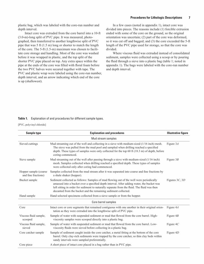
Table 1. Explanation of and procedures for different sample types.
[PVC, polyvinyl chloride]
Sample type Explanation and procedures Illustrative figure
Mud stream samples
Sieved cuttings Mud streaming out of the well and collecting in a sieve with medium-sized (1/16 inch) mesh. The sieve was pulled from the mud pool and sampled when drilling reached a specified depth. These types of samples were only collected for the top 60 ft (18.3 m) of depth, before coring commenced.
Figure 3A
Sieve sample Mud streaming out of the well after passing through a sieve with medium-sized (1/16 inch) mesh. Samples collected when drilling reached a specified depth. These types of samples were collected only after coring had commenced.
Figure 3B
Hopper sample (coarse and fine fractions)
Samples collected from the mud stream after it was separated into coarse and fine fractions by a shale shaker (hopper).
Bucket sample Sediment collected as follows: Samples of mud flowing out of the well were periodically amassed into a bucket over a specified depth interval. After adding water, the bucket was left sitting in order for sediment to naturally separate from the fluid. The fluid was then decanted from the bucket and the remaining sediment collected.
Figures 3C, 3D
Hand sample Hand selected specimens collected from a sieve sample or from the hopper.
Core barrel samples
Core Intact core or core segments that remained contiguous with one another in their original orien-tation as they were extruded into the lengthwise split of PVC pipe.
Figure 4A
Viscous fluid sample, scooped
Sample of water with suspended sediment or mud that flowed from the core barrel. High-viscosity samples were scooped directly into a plastic bag.
Figure 4B
Viscous fluid sample, sieved
Sample of water with suspended sediment or mud that flowed from the core barrel. Low-viscosity fluids were sieved before collecting in a plastic bag.
Figure 4C
Core catcher sample Sample of sediment caught inside the core catcher, a metal fitting at the bottom of the core barrel. Only clay-rich sediments were trapped by the core catcher, so thin clay beds within sandy intervals were sampled preferentially.
Figure 4D
Core piece A short piece of intact core placed in a bag rather than in PVC pipe.
plastic bag, which was labeled with the core-run number and depth interval.
Intact core was extruded from the core barrel into a 10-ft (3.0-m)-long split of PVC pipe. It was measured, photo-graphed, then transferred to another lengthwise split of PVC pipe that was 5 ft (1.5 m) long or shorter to match the length of the core. The 5-ft (1.5-m) maximum was chosen to facili-tate core storage and handling. Most of the core was washed before it was wrapped in plastic, and the top split of the shorter PVC pipe placed on top. Any extra space within the pipe at the ends of the core was filled with floral foam before the two PVC halves were secured together with tape. The PVC and plastic wrap were labeled using the core-run number, depth interval, and an arrow indicating which end of the core is up (shallowest).
In a few cases (noted in appendix 1), intact core was divided into pieces. The reasons include (1) forcible extrusion ended with some of the core on the ground, so the original orientation was uncertain; (2) part of the core was deformed, so it was cut off and bagged; and (3) the core exceeded the 5-ft length of the PVC pipe used for storage, so that the core was divided.
Where viscous fluid was extruded instead of consolidated sediment, samples were collected using a scoop or by pouring the fluid through a sieve into a plastic bag (table 1; noted in appendix 1). The bags were labeled with the core-run number and depth interval.

8 Sample Descriptions and Geophysical Logs for Cored Well, Great Sand Dunes National Park, Colorado
Figure 3. Photographs of various sampling procedures for mud stream samples. A, A cuttings sample is sieved and collected from the pool of mud next to the drill stem during the first 60 feet of rotary drilling. B, A sieve sample is collected from the mud stream while coring. The sieve, attached to a long handle, collects mud that is streaming up the sides of the core barrel and out of the hole. C, Mud streaming from the hole is collected periodically in a small bucket and emptied into a large bucket during the collection of a bucket sample. Pictured, left to right, Steve Grant and Jeff Eman, U.S. Geological Survey (USGS). D, At the end of the drilling interval, fluid from the large bucket is decanted and the remaining sediment stored as the bucket sample. Pictured, left to right, Jeff Eman and Harland Goldstein, USGS. Photographs by V.J.S. Grauch.

Procedures for Lithologic Descriptions 9
Figure 4. Photographs of various sampling procedures for core barrel samples. A, Intact core after extrusion onto a split half of polyvinyl chloride (PVC) pipe on a sawhorse apparatus. B, Viscous fluid collected with a shovel from poorly consolidated core that was extruded along with intact core (not shown). C, Viscous fluid poured through a sieve from the core barrel and collected as a sieved sample. D, Example of a core catcher sample before it was bagged. After detaching the core catcher at the bottom of the core barrel, sediment is inside the fixture and extending outside. Most other core catcher samples did not extend this far outside the fixture. Photographs by V.J.S. Grauch.

10 Sample Descriptions and Geophysical Logs for Cored Well, Great Sand Dunes National Park, Colorado
Effects of Storage and Handling
During the more than 4 years that samples were stored before examination, most of them dried out. Much of the clay making up the core samples contracted and broke into smaller pieces. Thus, the core was never split, fearing that such attempts would further disintegrate the samples. The bagged samples fared better; some of these retained a little of the original fluid that had been captured along with the sediment. Additional problems for the clay-rich samples were changes in color and biologic growth observed since acquisition, sug-gesting that chemical reactions had taken place. As a result, accurate color descriptions and chemical sampling were not attempted.
The desiccation and disaggregation of the clay-rich core samples affected measurements of core length between col-lection and examination. Shrinkage was most notable for the core samples containing the most clay, at depths below 261 ft (79.6 m). On the other hand, disaggregation of the desic-cated core also resulted in expansion of total length because
the pieces tended to separate and leave cracks between them. This problem is exacerbated by repeated handling of the core. Table 2 lists measured core lengths at original acquisition compared to two subsequent episodes of examination showing where core length has varied.
Photographs that capture how samples appeared at the drill site may be downloaded from the Photos folder, which also includes an index file describing the contents of the photographs. These photos are the best record of the condi-tions of the samples at the time they were collected, especially regarding color and sedimentary structures. Figure 5 shows an example of a clay-rich piece of core as it looked at the time of its collection compared to its appearance after more than 4 years of storage. Note the change in color and obscuring of oval blotches of different color that may be part of an impor-tant biogenic or sedimentary feature. Figure 6 demonstrates how the subtle color differences between samples from blue versus gray clay are obvious right after collection, but not so after they dried out.
Table 2. Core lengths recovered onsite in 2009 and changes in measured lengths in years 2012 and 2013.
[cm, centimeter; --, no data; %, percent]
Core run*Drilling depth
interval, in feet
Core length recovered in 2009,
in inches (cm)
2012 measured length,
in inches (cm)
2013 measured length,
in inches (cm)
2012 change from 2009
2013 change from 2009
9 125–128 12.0 (30.5) -- 12.0 (30.5) -- 0.0 %11 131–141 7.5 (19.1) 7.9 (20.0) 10.0 (25.4) +5.0 % +33 %13 171–191 47.0 (119.4) 47.2 (120.0) 48.0 (121.9) +0.5 % +2.1 %14 191–201 38.0 (96.5) 35.4 (90.0) 37.0 (94.0) –6.8 % –2.6 %15 210–211 20.0 (50.8) 20.1 (51.0) 20.0 (50.8) +0.4 % 0.0 %16 211–221 26. 0 (66.0) 24.8 (63.0) 26.0 (66.0) –4.6 % 0.0 %
17 (top) 231–241 57.5 (146.1) 55.9 (142.0) 57.5 (146.1) –2.8 % 0.0 %17 (bottom) 231–241 29.8 (75.6) 28.3 (72.0) 29.4 (74.7) –4.7 % –1.2 %
18 (top) 251–261 57.5 (146.1) 51.6 (131.0) 57.5 (146.1) –10 % 0.0 %18 (bottom) 251–261 17.0 (43.2) 13.8 (35.0) 17.0 (43.2) –19 % 0.0 %
19 261–266 54.0 (137.2) 45.7 (116.0) 48.0 (121.9) –15 % –11 %20 266–271 45.5 (115.6) 39.4 (100.0) 42.0 (106.7) –13 % –7.7 %21 271–276 44.0 (111.8) 35.4 (90.0) 38.0 (96.5) –20 % –14 %22 276–291 11.0 (27.9) 9.1 (23.0) 10.0 (25.4) –18 % –9.1 %23 291–301 59.0 (149.9) 57.9 (147.0) 60.0 (152.4) –1.9 % +1.7 %24 301–306 60.0 (152.4) 56.3 (143.0) 60.0 (152.4) –6.2 % 0.0 %25 306–311 24.0 (61.0) 22.8 (58.0) 23.0 (58.4) –4.9 % –4.2 %26 311–316 57.0 (144.8) 54.3 (138.0) 54.0 (137.2) –4.7 % –5.3 %27 316–321 60.0 (152.4) 53.2 (135.0) 54.0 (137.2) –11 % –10 %28 321–326 55.0 (139.7) 49.6 (126.0) 52.0 (132.1) –9.8 % –5.5 %
*Core was not recovered from all core runs. Cores recovered from runs 17 and 18 were divided into top and bottom pieces on site and stored separately.

Procedures for Lithologic Descriptions 11
Figure 5. Photographs of a selected core at time of collection compared to more than 4 years later. A, Washed core piece from the bottom of core run 25 (depths 306–311 ft) on September 17, 2009. Note the dark oval splotch that may be a sedimentary structure or trace fossil. B, The same core piece as it looked on February 5, 2014, after it had been wrapped in plastic and stored inside a polyvinyl chloride (PVC) pipe. Note the color change, breakage, and difficulty seeing the oval splotch. Photographs by V.J.S. Grauch (A) and Gary L. Skipp (B).

12 Sample Descriptions and Geophysical Logs for Cored Well, Great Sand Dunes National Park, Colorado
Figure 6. Photographs of two clay samples of differing color at time of collection in September 2009 compared to almost 5 years later in August 2014. A, Clay with blue tint at time of collection as a core catcher sample at 266 ft depth (core run 19). B, Clay with even-gray color at time of collection from ≈311 ft depth (core run 26). C, Clay from the same sample as in A after almost 5 years of storage in a plastic bag. Note the color change. D, Clay from the same core sample as in B after almost 5 years of storage wrapped in plastic in a polyvinyl chloride (PVC) pipe. Note the extensive disaggregation and the color change for a small piece of the core on the right-hand side of the photo. Photographs by V.J.S. Grauch (A and B) and Gary L. Skipp (C and D).

Procedures for Lithologic Descriptions 13
Laboratory Methods
All samples from the well were examined and described regarding grain sizes, types, and shapes; sorting, layering, and sedimentary structures; calcium carbonate content; occurrence of fossils or other biogenic material; evidence of biologic activity such as trace fossils or bioturbation; and presence of volcanic ash (appendix 1). Some samples were examined for mineralogy using X-ray diffraction analysis. Difficulties in sample recovery and the effects caused by the long period of sample storage affect how well these descriptions actually represent the lithology at depth. Specific depths that were sampled are uncertain for core samples that are shorter in length than the drilling depth interval.
Bagged samples from the drilling and coring were first identified as to type of sample (table 1). Cores were first wet-ted with a spray bottle then scraped to a depth of several milli-meters on a portion of the core over the entire length. Scraping was done to remove core barrel smear contamination. Wetting was done for visual enhancement of any structures present (bedding, laminations, faulting, bioturbation, contacts, grain size changes, and so forth). Because some of the core had fragmented, a representative piece within broken intervals was chosen for wetting and scraping.
Both bagged and core samples were then examined under a binocular microscope to observe grain size and shape, sort-ing, grain color, and some mineralogy. The relative quantity of calcium carbonate (calcareous degree) was estimated from the intensity of effervescence after application of a 10-percent solution of hydrochloric acid (HCl). Core samples were tested every few inches. Samples suspected to contain fossils or unusual mineral assemblages were viewed under the binocu-lar microscope. Some such samples were tested for magnetic grains using a magnet. Several samples were chosen for X-ray diffraction analysis to determine mineralogy. A subset of these samples were mounted (smear slide) for petrographic examination.
Occurrences of animal remains and evidence of bio-logic activity were noted during the systematic examination of bagged and core samples in 2013 by G.L. Skipp and by M.E. Benson and J.K. Davis while studying core samples in 2012. Most fossil specimens were categorized as bivalves, gastropods, ostracods, or unidentified shells. A few samples were examined by M.E. Benson for the potential presence of diatoms. Where diatoms were found, they were preliminarily identified. Bones and teeth were distinguished, where possible, but no effort was made to identify the animal type, as remains were not intact. Other evidence of animal or plant life included fine organic debris, woody plant parts, or bioturbation, none of which was researched in detail. Appendix 2 provides descrip-tions of the fossils or other evidence of life and the depth intervals where they were observed. Because core length measurements differed between the 2012 and 2013 studies, the locations of the occurrences within the core samples are listed separately and should be considered approximate for future work.
Samples taken for X-ray diffraction analysis were ground to <200 mesh size (≈10 micrometer [μm]) and packed into a cavity mount. Analysis was performed on a Philips R150 goni-ometer with a XRG3100 generator using a 2°-theta scan range of 6–65. Resulting X-ray diffraction patterns were evaluated for characteristic patterns of common minerals. The resulting bulk mineralogy for each sample is listed in appendix 3.
Sample Descriptions Versus Well DepthsFindings from the sample descriptions detailed in appen-
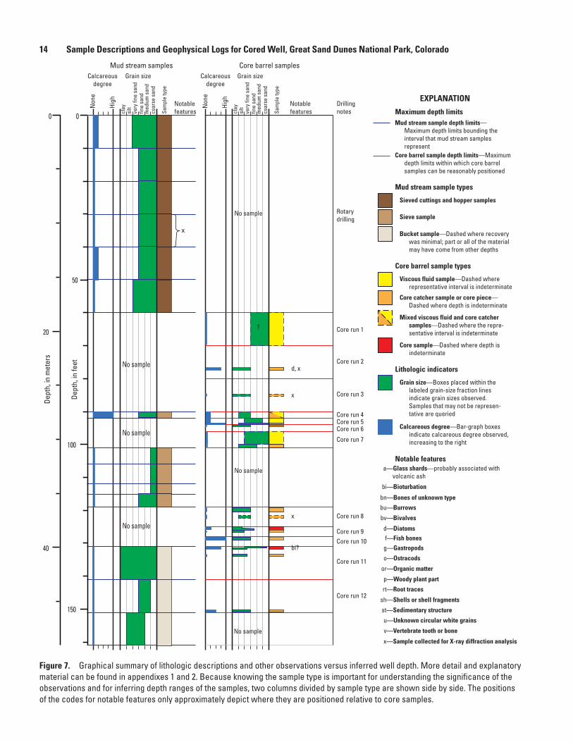
dix 1 are depicted graphically versus well depth in figure 7, divided in two columns by sample type. Assigning the findings to specific depths within the well is not straightforward due to uncertainties caused by poor core recovery and difficulties in sampling sands. The uncertainties, and thus how depths were estimated, are different for mud stream versus core bar-rel samples. For mud stream samples collected over specific depth intervals, uncertainties arose as to whether they accu-rately represent the sediment in the well over that interval. For core samples that were shorter than their associated drilling interval, uncertainties arose regarding their positions within that interval.
Mud stream samples collected during the first 60 ft of rotary drilling (sieved cuttings and hopper samples) were obtained as cuttings of all sediment and are considered to adequately represent the intervals they sampled. Below this depth, sieve and bucket samples were also collected for speci-fied depth intervals, but the sediment may not adequately represent the sediment within that depth interval because of possibilities of mixing with sediment from uphole depths. On the other hand, the volume retrieved in bucket samples sig-nificantly decreased as more clay was recovered as core. This correlation, along with very similar lithology noted for these minimal-volume samples, suggests that the quantity of con-taminating material was limited. In any case, bucket samples with minimal volume are not reliable samples, because they may not be representative of the depth interval sampled, and are noted with question marks on figure 7.
Depth placement of most core samples was evaluated using matches of the lithology of the sample to the description of sediment encountered in the interval onsite and support-ing evidence from the geophysical logs. Some matches relied primarily on the geophysical logs. Depth intervals of core could also be estimated relative to the underlying core catcher sample. Depths were generally easier to estimate for core catcher samples because they commonly represented the last clay recognized by drilling speed before the driller pulled the core barrel. In all but one case, core that was extruded from the barrel in pieces could be considered contiguous. The one exception is core run 13 (depth interval 171–191 ft), where core was extruded as many pieces (4-ft total length) along with viscous fluid (appendix 1 and fig. 7). If the many pieces were considered contiguous, the clay and cemented sand layers observed did not match in depth compared with relative low- versus high-resistivity values in the geophysical logs. The matches were improved if a gap in core recovery was inferred.
14 Sample Descriptions and Geophysical Logs for Cored Well, Great Sand Dunes National Park, Colorado
Figure 7. Graphical summary of lithologic descriptions and other observations versus inferred well depth. More detail and explanatory material can be found in appendixes 1 and 2. Because knowing the sample type is important for understanding the significance of the observations and for inferring depth ranges of the samples, two columns divided by sample type are shown side by side. The positions of the codes for notable features only approximately depict where they are positioned relative to core samples.
Calcareousdegree
Calcareousdegree
Grain sizeGrain size
Mud stream samples Core barrel samples
Non
e
High
Non
e
High
silt
coar
se s
and
med
ium
san
dfin
e sa
ndve
ry fi
ne s
and
clay
silt
coar
se s
and
med
ium
san
dfin
e sa
ndve
ry fi
ne s
and
clay
Rotary drilling
Core run 1
Core run 2
Core run 4Core run 5Core run 6
Core run 7
Core run 8
Core run 9Core run 10
Core run 11
Core run 12
Core run 3
No sample
No sample
No sample
Drillingnotes
?
Sieved cuttings and hopper samples
Sieve sample
Bucket sample—Dashed where recovery was minimal; part or all of the material may have come from other depths
EXPLANATION
Mud stream sample types
Viscous fluid sample—Dashed where representative interval is indeterminate
Core catcher sample or core piece—Dashed where depth is indeterminate
Core sample—Dashed where depth is indeterminate
Core barrel sample types
Maximum depth limits
Grain size—Boxes placed within the labeled grain-size fraction lines indicate grain sizes observed. Samples that may not be represen-tative are queried
Calcareous degree—Bar-graph boxes indicate calcareous degree observed, increasing to the right
Lithologic indicators
Mixed viscous fluid and core catcher samples—Dashed where the repre-sentative interval is indeterminate
Sam
ple
type
Sam
ple
type
a—Glass shards—probably associated with volcanic ash
bn—Bones of unknown type
bu—Burrows
bv—Bivalves
g—Gastropods
o—Ostracods
p—Woody plant part
f—Fish bones
or—Organic matter
sh—Shells or shell fragments
st—Sedimentary structure
u—Unknown circular white grains
v—Vertebrate tooth or bone
x—Sample collected for X-ray diffraction analysis
rt—Root traces
d—Diatoms
Notable features
Notable features
Mud stream sample depth limits—Maximum depth limits bounding the interval that mud stream samples represent
Core barrel sample depth limits—Maximum depth limits within which core barrel samples can be reasonably positioned
Notable features
d, x
bi?
x
x
x
No sample
No sample
No sample
0
20
40
Dept
h, in
met
ers
0
50
150
100
Dept
h, in
feet
bi—Bioturbation
Procedures for Lithologic Descriptions 15
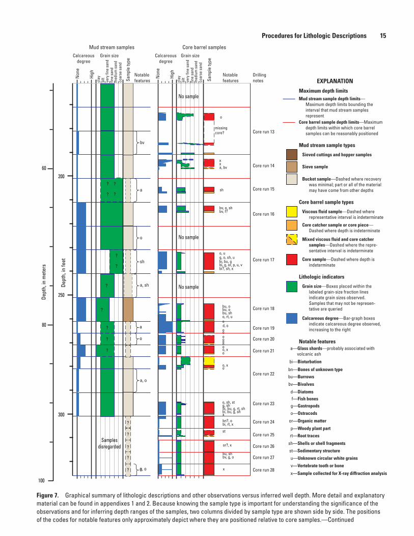
Figure 7. Graphical summary of lithologic descriptions and other observations versus inferred well depth. More detail and explanatory material can be found in appendixes 1 and 2. Because knowing the sample type is important for understanding the significance of the observations and for inferring depth ranges of the samples, two columns divided by sample type are shown side by side. The positions of the codes for notable features only approximately depict where they are positioned relative to core samples.—Continued
Non
e
High
Calcareousdegree
Non
e
High
Grain size Calcareousdegree
Grain size
Mud stream samples Core barrel samples
silt
coar
se s
and
med
ium
san
dfin
e sa
ndve
ry fi
ne s
and
clay
silt
coar
se s
and
med
ium
san
dfin
e sa
ndve
ry fi
ne s
and
clay
Core run 13
Core run 14
Core run 15
Core run 16
Core run 17
Core run 18
Core run 19
Core run 20
Core run 21
Core run 22
Core run 23
Core run 24
Core run 25
Core run 26
Core run 27
Core run 28
Drillingnotes
?
?
?
?
?
?
?
?
?
?
?
?
?
?
?
?
missingcore?
Sam
ple
type
Sam
ple
type
Notable features
Notable features
o
bv
o
a
sh
a, sh
a, o
a
o
og, o
a, bv
bv, o, shbv, f?
sh
o, ug, o, sh, u
bi, g, or, p, u, vbi?, sh, x
bi, bu, g
bu, o
bu, shbu, o
o, rt, uod, ooooooooo, xo
oo, x
o, sh, stg, sh
bi, bu, g, shbi, bu, g, rt, sh
bn?, o
st
bv, g, obu, sh
xx
x
bi, rt, x
or?, x
x
Samplesdisregarded
No sample
No sample
No sample
60
80
100
Dept
h, in
met
ers
200
250
300
Dept
h, in
feet
Sieved cuttings and hopper samples
Sieve sample
Bucket sample—Dashed where recovery was minimal; part or all of the material may have come from other depths
EXPLANATION
Mud stream sample types
Viscous fluid sample—Dashed where representative interval is indeterminate
Core catcher sample or core piece—Dashed where depth is indeterminate
Core sample—Dashed where depth is indeterminate
Core barrel sample types
Maximum depth limits
Grain size—Boxes placed within the labeled grain-size fraction lines indicate grain sizes observed. Samples that may not be represen-tative are queried
Calcareous degree—Bar-graph boxes indicate calcareous degree observed, increasing to the right
Lithologic indicators
Mixed viscous fluid and core catcher samples—Dashed where the repre-sentative interval is indeterminate
a—Glass shards—probably associated with volcanic ash
bn—Bones of unknown type
bu—Burrows
bv—Bivalves
g—Gastropods
o—Ostracods
p—Woody plant part
f—Fish bones
or—Organic matter
sh—Shells or shell fragments
st—Sedimentary structure
u—Unknown circular white grains
v—Vertebrate tooth or bone
x—Sample collected for X-ray diffraction analysis
rt—Root traces
d—Diatoms
Mud stream sample depth limits—Maximum depth limits bounding the interval that mud stream samples represent
Core barrel sample depth limits—Maximum depth limits within which core barrel samples can be reasonably positioned
Notable features
bi—Bioturbation
16 Sample Descriptions and Geophysical Logs for Cored Well, Great Sand Dunes National Park, Colorado
Most depth estimates have fair confidence. Those with uncertainties are indicated by dashed outlines on figure 7. In all cases, maximum errors on the position of the core samples are defined by the upper and lower limits of the drilling depth interval (red lines on fig. 7). Uncertainties for three core runs are particularly large, for which the maximum errors apply (runs 3, 13, and 14; fig. 7).
The depths that viscous fluid samples represent are all uncertain, so all outlines for these sample types are dashed on figure 7. Although the fluid must have sampled the depth interval indicated, it is likely that the entire volume of that interval is not adequately represented. In some cases, the relation of the viscous fluid to more solid portions of the core barrel sample was obvious after extrusion from the barrel, so the depth uncertainties are somewhat less.
Geophysical LogsSix wireline geophysical tools were used to obtain logs
of natural gamma-ray, electrical resistivity and conductivity, spontaneous potential, full waveform sonic, density, and neu-tron data and several other borehole parameters. These logs were chosen to augment lithologic interpretations of the well and to investigate physical properties of the subsurface that can be correlated to surface geophysical measurements and to other wells in the region.
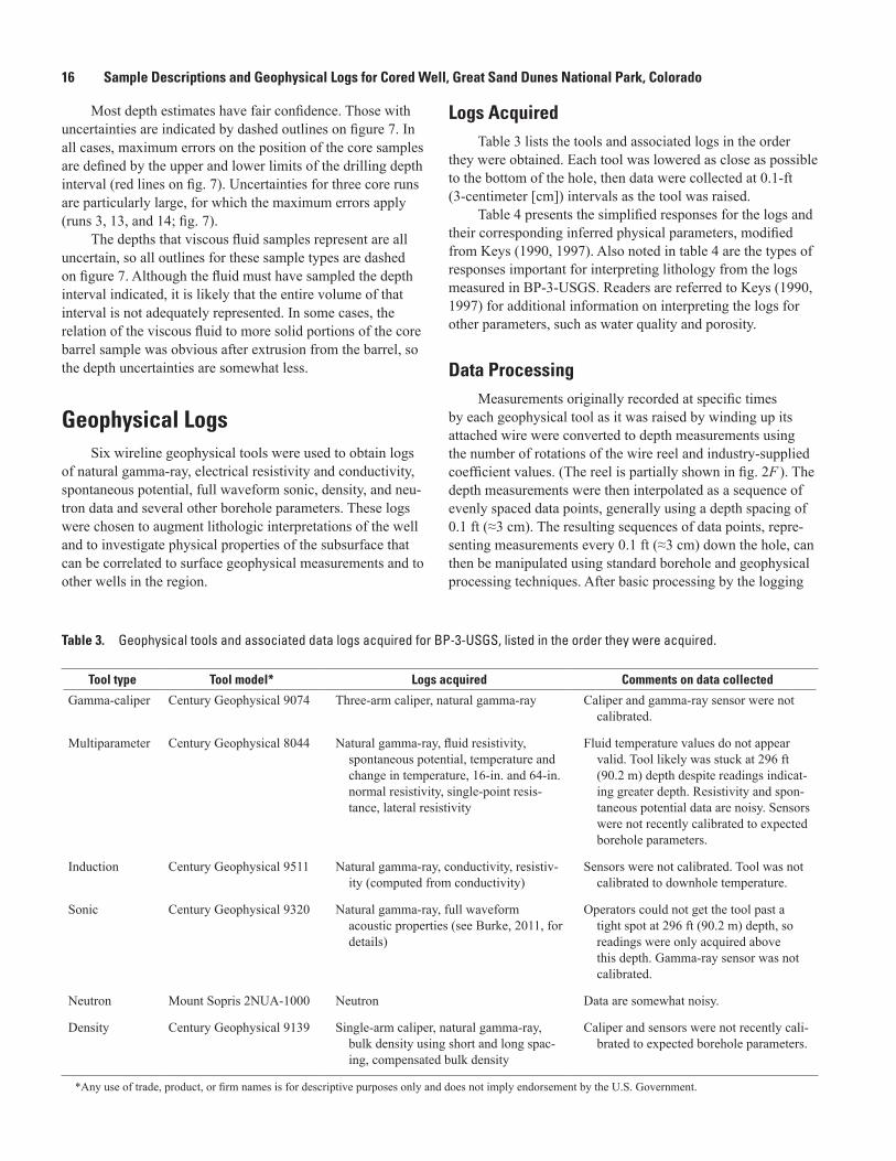
Logs AcquiredTable 3 lists the tools and associated logs in the order
they were obtained. Each tool was lowered as close as possible to the bottom of the hole, then data were collected at 0.1-ft (3-centimeter [cm]) intervals as the tool was raised.
Table 4 presents the simplified responses for the logs and their corresponding inferred physical parameters, modified from Keys (1990, 1997). Also noted in table 4 are the types of responses important for interpreting lithology from the logs measured in BP-3-USGS. Readers are referred to Keys (1990, 1997) for additional information on interpreting the logs for other parameters, such as water quality and porosity.
Data ProcessingMeasurements originally recorded at specific times
by each geophysical tool as it was raised by winding up its attached wire were converted to depth measurements using the number of rotations of the wire reel and industry-supplied coefficient values. (The reel is partially shown in fig. 2F ). The depth measurements were then interpolated as a sequence of evenly spaced data points, generally using a depth spacing of 0.1 ft (≈3 cm). The resulting sequences of data points, repre-senting measurements every 0.1 ft (≈3 cm) down the hole, can then be manipulated using standard borehole and geophysical processing techniques. After basic processing by the logging
Table 3. Geophysical tools and associated data logs acquired for BP-3-USGS, listed in the order they were acquired.
Tool type Tool model* Logs acquired Comments on data collected
Gamma-caliper Century Geophysical 9074 Three-arm caliper, natural gamma-ray Caliper and gamma-ray sensor were not calibrated.
Multiparameter Century Geophysical 8044 Natural gamma-ray, fluid resistivity, spontaneous potential, temperature and change in temperature, 16-in. and 64-in. normal resistivity, single-point resis-tance, lateral resistivity
Fluid temperature values do not appear valid. Tool likely was stuck at 296 ft (90.2 m) depth despite readings indicat-ing greater depth. Resistivity and spon-taneous potential data are noisy. Sensors were not recently calibrated to expected borehole parameters.
Induction Century Geophysical 9511 Natural gamma-ray, conductivity, resistiv-ity (computed from conductivity)
Sensors were not calibrated. Tool was not calibrated to downhole temperature.
Sonic Century Geophysical 9320 Natural gamma-ray, full waveform acoustic properties (see Burke, 2011, for details)
Operators could not get the tool past a tight spot at 296 ft (90.2 m) depth, so readings were only acquired above this depth. Gamma-ray sensor was not calibrated.
Neutron Mount Sopris 2NUA-1000 Neutron Data are somewhat noisy.
Density Century Geophysical 9139 Single-arm caliper, natural gamma-ray, bulk density using short and long spac-ing, compensated bulk density
Caliper and sensors were not recently cali-brated to expected borehole parameters.
*Any use of trade, product, or firm names is for descriptive purposes only and does not imply endorsement by the U.S. Government.

Geophysical Logs 17
Table 4. Description of geophysical logs and their utility for BP-3-USGS.
[PVC, polyvinyl chloride]
Log type Parameters measuredPhysical parameters
inferredNotes important for lithologic interpretation of
BP-3-USGS
Caliper Hole diameter Wash-outs or restric-tions of the sides of the hole
Integrity of the well bore gives clues regarding sand versus clay intervals. Geophysical measurements in wash-outs may be affected and not representative of the formation.
Natural gamma Natural-gamma radiation Clay or feldspar content
Radiation increases with increasing clay or increasing potassium associated with abundance of feldspar, such as in volcanic sands. Readings are attenuated inside PVC casing.
Normal resistivity Electrical resistivity of formation plus pore and borehole fluids, measured over sensor spacings of 16 in. and 64 in.
Lithology, bed bound-aries, and water quality
Resistivity generally decreases with increasing clay content. The 64-in. (long-normal) sensor samples greater volume of material vertically and laterally into the formation than does the 16-in. (short-normal) sensor, resulting in a 64-in. normal curve that is much smoother than the 16-in. normal curve. Readings are affected by borehole fluid and are not valid inside the PVC casing.
Induction Conductivity induced from electromagnetic fields
Lithology and bed boundaries
Resistivity curves computed as the inverse of conductiv-ity data are complimentary to the normal resistivity curves and provide similar information. Readings are unaffected by PVC casing and are more impervious to borehole effects than the normal resistivity sensors.
Spontaneous potential Natural electrical poten-tials
Lithology, bed bound-aries, and water quality
Curve inflections correspond to contacts between beds of different lithology. Readings are not valid inside PVC casing.
Sonic Travel time of an acous-tic wave between transmitters and receivers
Sonic velocity and porosity
The sonic tool was chosen for BP-3-USGS to get a general sense of the overall sonic velocity of poorly consolidated sediments in this region. The readings are attenuated inside PVC casing.
Neutron Neutrons slowed and scattered by hydrogen
Saturated porosity Increasing counts correspond to increasing volume of fluid-filled pore spaces. Porosity and pore connectivity commonly reflect differences in lithology. Clays may have higher porosity than sands, but the pores are not connected, so the effective porosity is low. The read-ings are attenuated inside PVC casing.
Density Scattered and attenuated gamma photons
Bulk density and porosity
The density tool was chosen for BP-3-USGS to get a general sense of the overall bulk density of poorly consolidated sediments in this region. The readings are attenuated inside PVC casing.
operator, we additionally checked the data for depth calibra-tion, applied routines to eliminate spurious data and attenuate noise, adjusted for tool calibration problems, and corrected for effects of borehole fluid and hole diameter. These steps are described in the following sections. Description of the more extensive data processing of the sonic log is described in Burke (2011). Table 5 summarizes the types of processing applied for each log.
Common to the data processing of many of the geophysi-cal logs was the application of spike-rejection and low-pass filters, as implemented by Geosoft OASIS for a sequence of evenly spaced data points. Data spikes were removed using a nonlinear filter, based on a procedure described by Naudy and Dreyer (1968). The filter rejects data points that exceed a particular amplitude tolerance over a certain specified depth interval and replaces them with an estimate based on
18 Sample Descriptions and Geophysical Logs for Cored Well, Great Sand Dunes National Park, Colorado
Table 5. Overview of data processing steps applied to geophysical logs.
[PVC, polyvinyl chloride]
Log type Data editing Filters applied Corrections applied
Three-arm caliper None None Shifted to match expected readings inside PVC casing, which has fixed diameter.
Natural gamma(five different tools)
None Low-pass None.
Normal resistivity Remove data measured within PVC casing and depths at bottom, below where the tool was stuck
Spike-rejection and low-pass
Corrected for borehole effects.
Resistivity from induction None Low-pass Scaled to 16-in. normal resistivity curve.
Spontaneous potential Remove data measured within PVC casing
Spike-rejection and low-pass
None.
Sonic None See Burke (2011) See Burke (2011).
Neutron None Spike-rejection and low-pass
Rescale depth to match other tools.
Density None Low-pass Calibration correction.
surrounding data points. We chose amplitude tolerances of about 1.33 percent of the total range of data values and used a depth interval that spans three data points, or an interval of 0.3 ft (9 cm). Low-pass filters were applied to smooth the data, using a convolution filter as described by Fraser and others (1966). The low-pass filter is designed to remove all features of the log trace that have wavelengths less than a designated cutoff wavelength. The filter is tapered using a taper length equal to the wavelength cutoff distance so that side effects of the filtering are minimized. For the BP-3-USGS geophysical logs, we used a wavelength cutoff that spans 20 data points, or a depth interval of 2 ft (0.61 m), except for the normal resistiv-ity logs where a wavelength cutoff spanning 10 points, or a depth interval of 1 ft (0.30 m), was applied.
Check of Depth Calibration
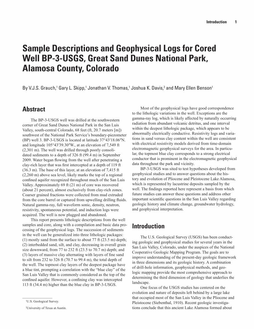
Although natural gamma-ray logs are commonly used to distinguish different lithologies, comparing gamma-ray logs from multiple runs can also help evaluate calibration of depth between logs. Although the amplitudes and details of the gamma-ray curves in counts per second (cps) are expected to vary for each run of the different tools, general features should line up if depth is calibrated correctly. Figure 8 compares the three-arm caliper log and low-pass-filtered, natural gamma-ray logs from five different tools. The caliper records the diameter of the hole through which the tool passed to identify tight spots and wash-outs. Two wash-outs apparent from the wide excursions of the caliper measurements at 80 ft (24.4 m) and 130 ft (39.6 m) are accompanied by abrupt drops in all the gamma-ray curves. Although the wash-outs indicate the
geophysical tools were not correctly measuring parameters of the lithology, the drop-outs in the gamma readings are well aligned, indicating that the depth scales on these logs are well calibrated.
The overall shapes of the gamma-ray curves are well matched throughout most of the length of the well confirm-ing that depth is well calibrated between logs. One exception comes from comparing the curves for depths below the tight spot at 296 ft (90.2 m) where the caliper reading reaches less than 4 in. (10 cm). Operators had difficulties getting most of the tools below this point; they abandoned attempts for the sonic tool. However, the multiparameter tool may not have reached the bottom of the hole as well, as evident below this point from a moderate decrease in tension (downloads direc-tory), a lack of character in the multiparameter gamma-ray curve, and flat-lined resistivity readings (not shown). These observations suggest that the multiparameter tool was stuck at this tight spot. Therefore, data were eliminated from the logs appropriate to where each of the sensors was located on the probe when it reached 296 ft (90.2 m).
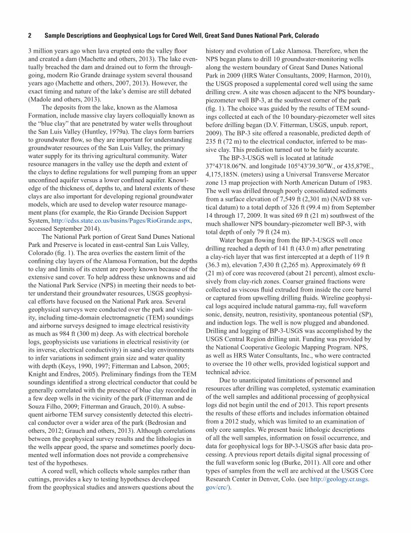
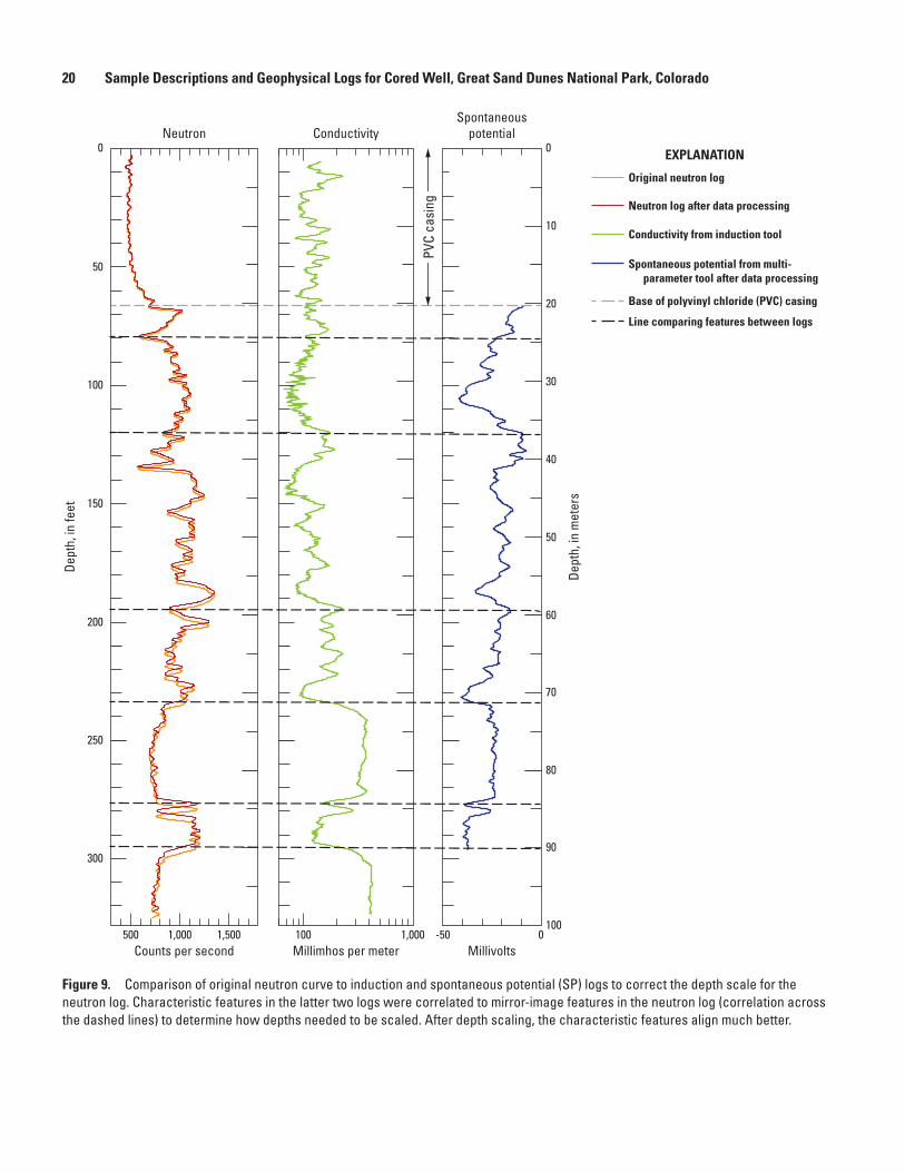
Because the neutron tool did not include a natural gamma-ray detector, the neutron log was compared to the induction and SP logs to check depth calibration (fig. 9). After application of spike-rejection and low-pass filters to all three logs, many individual features of these curves were similar or mirror images of each other and thus should occur at the same depth. Instead, characteristic features of the neutron curve, indicated at several places on figure 9 by the dashed lines that cross all three logs, appear to be shifted in depth. Because the neutron tool was the only model produced by Mount Sopris rather than Century Geophysical (table 3), the depth offset of the neutron curve may be due to differences in the coefficient

Geophysical Logs 19
Figure 8. Borehole diameter measured by the three-arm caliper and low-pass-filtered, natural gamma-ray curves from five different tools. Note that the curves are stacked using a relative scale; their absolute values are floating.
4
2 51 3100 200
Counts per second
Caliper
Hole diameter, inches
Dept
h, in
feet
EXPLANATION
Filtered gamma reading
Gamma-caliper tool
Induction tool
Sonic tool
Multiparameter tool
Density tool
Base of polyvinyl chloride (PVC) casing
Dept
h, in
met
ers
0.0 10.0 20.0
5
321
410
20
30
50
70
90
0
50
150
200
250
300
100
0
50
150
200
250
300
100
0
40
60
80
100
10
20
30
50
70
90
0
40
60
80
100
PVC
casi
ng
20 Sample Descriptions and Geophysical Logs for Cored Well, Great Sand Dunes National Park, Colorado
Figure 9. Comparison of original neutron curve to induction and spontaneous potential (SP) logs to correct the depth scale for the neutron log. Characteristic features in the latter two logs were correlated to mirror-image features in the neutron log (correlation across the dashed lines) to determine how depths needed to be scaled. After depth scaling, the characteristic features align much better.
EXPLANATION
100 1,000
Original neutron log
500 1,000 1,500Counts per second
0
50
150
200
250
300
100
-50 0
Dept
h, in
feet
0
20
40
60
80
100
Dept
h, in
met
ers
Line comparing features between logs
Neutron log after data processing
Conductivity from induction tool
Spontaneous potential from multi-parameter tool after data processing
Base of polyvinyl chloride (PVC) casing
Conductivity
Millimhos per meter
NeutronSpontaneous
potential
Millivolts
10
30
50
70
90
PVC
casi
ng

Geophysical Logs 21
values used by the two companies to determine depth from the number of rotations of the wire reel. A scaling factor of 0.992, determined by inspection, was multiplied to the depth values of the neutron log to fix the problem. The neutron curves before (orange line) and after (red line) correcting the depth scale are shown on figure 9.
Normal Resistivity LogsNormal resistivity logs need to be corrected for borehole
effects to obtain more representative measurements of the resistivity of the formation. Borehole effects include the resis-tivity of the drilling fluid, borehole diameter, volume of fluid invasion, and bed thickness (Keys, 1990, 1997). Scott (1978) presented a practical algorithm for correcting normal resistiv-ity log data for borehole diameter and mud resistivity. The algorithm is derived from resistivity departure-curve charts developed earlier by Schlumberger Well Surveying Corpora-tion, assuming no invasion of drilling mud and an infinite bed thickness. The validity of these assumptions is difficult to ascertain for BP-3-USGS, but they likely are not met. The cor-rection was applied anyway, assuming it improves the results more than no correction at all.
Figure 10 shows the normal resistivity curves before and after correction and filtering. The correction used equation 2 of Scott (1978), incorporating a tool diameter of 2.1 in. (5.3 cm) and fluid resistivity values taken from those measured during the logging. Resistivities of the fluid varied little through-out the hole, ranging from 5.9 to 6.2 ohm-meter (ohm-m). The fluid was probably well distributed throughout the hole because of the artesian flow. Spike-rejection and low-pass fil-ters were then applied to the corrected normal resistivity data. The low-pass filter used a wavelength cutoff spanning 10 data points (or a depth interval of 1 ft, 0.3 m).
Induction LogConductivity readings from the induction tool were
inverted to resistivity values for comparison to the normal resistivity logs (fig. 11). The resulting resistivities appeared much too low, likely due to tool calibration problems. On the other hand, individual features of the induction curve show remarkable similarity to the 16-in. normal resistivity curve. Scatter plots comparing resistivity values for the two curves show a linear relation below 120 ft (36.5 m) but no observ-able relation shallower than this depth. Thus, to adjust for the calibration problem, the induction-tool resistivity values were scaled using a match to the 16-in. normal curve below 120 ft (36.5 m) depth as the criteria. The resulting transform applied to the induction-tool resistivity Rind to get a corrected Rcorr was computed in ohm-meters as
Rcorr = 3.75 Rind + 3.3.
Figure 11 shows the resistivity curves from the induction tool before and after scaling and after a low-pass filter was applied. The curves are shown in comparison to the normal resistivity curves after they were corrected and filtered.
Why the induction-tool resistivities and the normal resistivities have no apparent relation shallower than 120 ft (36.5 m) is unknown. Resistivities derived from a time-domain electromagnetic (TEM) sounding that was measured at the site before drilling suggest the problem lies with the induction log (fig. 12). The TEM model (D.V. Fitterman, USGS, unpub. data, 2009) is derived by assuming there are only four layers of different resistivity in the subsurface. The resistivities of each model layer, depicted by the straight vertical lines on figure 12, are a broad representation of the resistivities of the formation and pore fluids together. The TEM model matches the borehole resistivity curves fairly well below the depth of 120 ft (36.5 m). The TEM model matches the normal resistiv-ity curves better than the induction-tool resistivity curve above this depth. Interestingly, the 120-ft depth is close to the top of the confining clay layer at 119 ft (36.3 m), suggesting that the explanation is related to differences in the formation fluids in the unconfined and confined aquifers. However, this line of reasoning is contradicted by considering that borehole fluid affects the normal resistivity measurements more than those of the induction tool (table 4).
Density and Sonic LogsAfter reviewing the original readings from the two den-
sity sensors (short-spaced and long-spaced), it was determined that density values were too low for the known lithology, and the tool calibration was not accurate. In 2013, the two sensors were calibrated at the USGS Texas Water Science Center in Austin, Texas, by measuring two reference blocks with known densities (aluminum and nylon with densities of 2.62 grams per cubic centimeter [g/cm3] and 1.24 g/cm3, respectively). This new calibration was then applied to the original log to provide an accurate, compensated bulk density log. A low-pass filter was applied to the compensated density log resulting from the calibration, which is shown in figure 13 alongside the sonic (seismic P-wave) velocity derived from the full wave-form sonic log by Burke (2011). These density and sonic logs are best used to provide average values of bulk density and sonic velocity for shallow sediments of the San Luis Valley as opposed to detailed information about variations in lithology in the well. Sonic velocities average 5,922 ft/s (1,805 m/s) (Burke, 2011), with a standard deviation of 230 ft/s (70 m/s). The average and standard deviation from the compensated density log, not considering excursions at 80 and 135 ft (24.4 and 41.4 m) and values measured within the PVC casing, are 1.97 g/cm3 (1,970 kilograms per cubic meter [kg/m3]) and 0.12 g/cm3 (120 kg/m3), respectively. These measurements are compatible with Gardner’s empirical relation between sonic velocity and bulk density in sedimentary basins (Gard-ner and others, 1974), in which a sonic velocity of 5,922 ft/s (1,805 m/s) relates to a density of 2.02 g/cm3 (2,020 kg/m3).
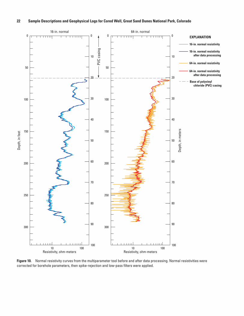
22 Sample Descriptions and Geophysical Logs for Cored Well, Great Sand Dunes National Park, Colorado
Figure 10. Normal resistivity curves from the multiparameter tool before and after data processing. Normal resistivities were corrected for borehole parameters, then spike-rejection and low-pass filters were applied.
EXPLANATION
10 100
16-in. normal
10 100
64-in. normal0
40
60
80
100
0
50
0
50
150
200
250
300
100
150
200
250
300
100
Resistivity, ohm-meters Resistivity, ohm-meters
10
30
50
70
90
0
40
60
80
100
10
20 20
30
50
70
90
64-in. normal resistivity
64-in. normal resistivity after data processing
16-in. normal resistivity
16-in. normal resistivity after data processing
Base of polyvinyl chloride (PVC) casing
Dept
h, in
feet
Dept
h, in
met
ers
PVC
casi
ng
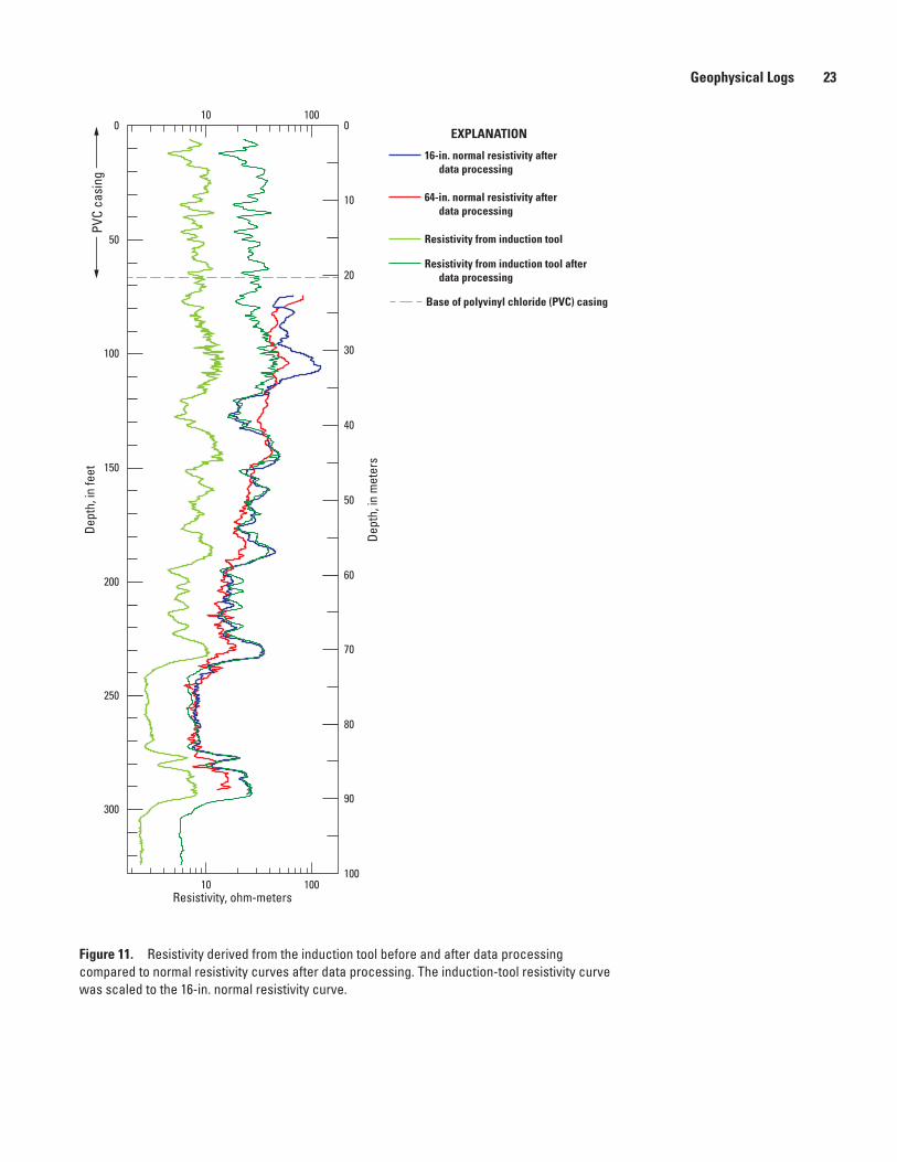
Geophysical Logs 23
Figure 11. Resistivity derived from the induction tool before and after data processing compared to normal resistivity curves after data processing. The induction-tool resistivity curve was scaled to the 16-in. normal resistivity curve.
10 100
10 1000
50
150
200
250
300
100
Resistivity, ohm-meters
0
40
60
80
100
10
20
30
50
70
90
Dept
h, in
met
ers
PVC
casi
ng
EXPLANATION
Resistivity from induction tool after data processing
64-in. normal resistivity after data processing
Resistivity from induction tool
16-in. normal resistivity after data processing
Base of polyvinyl chloride (PVC) casing
Dept
h, in
feet

24 Sample Descriptions and Geophysical Logs for Cored Well, Great Sand Dunes National Park, Colorado
Figure 12. Resistivity curves after data processing compared to resistivity layers derived from a time-domain electromagnetic (TEM) sounding measured at the site before drilling (D.V. Fitterman, U.S. Geological Survey, unpub. data, 2009). The TEM model is derived by assuming there are only four layers of different resistivity in the subsurface.
EXPLANATION
Resistivity from induction tool after data processing
64-in. normal resistivity after data processing
16-in. normal resistivity after data processing
Model from transient electro-magnetic (TEM) sounding
Base of polyvinyl chloride (PVC) casing
0
50
150
200
250
300
100
Resistivity, ohm-meters
0
40
60
80
100
10
20
30
50
70
90
Dept
h, in
met
ers
PVC
casi
ng
10 100 1,000
Dept
h, in
feet

Geophysical Logs 25
Figure 13. Sonic velocity and compensated density logs.
EXPLANATION
1,500 2,500Meters per second
Sonic
1.00 2.00Grams per cubic
centimeter
Density
Dept
h, in
met
ers
Dept
h, in
feet
Compressional sonic velocity derived from sonic log from Burke (2011)
Compensated density log after data processing
Base of polyvinyl chloride (PVC) casing
0
150
200
250
300
100
0
40
60
80
100
10
20
30
50
70
90
PVC
casi
ng
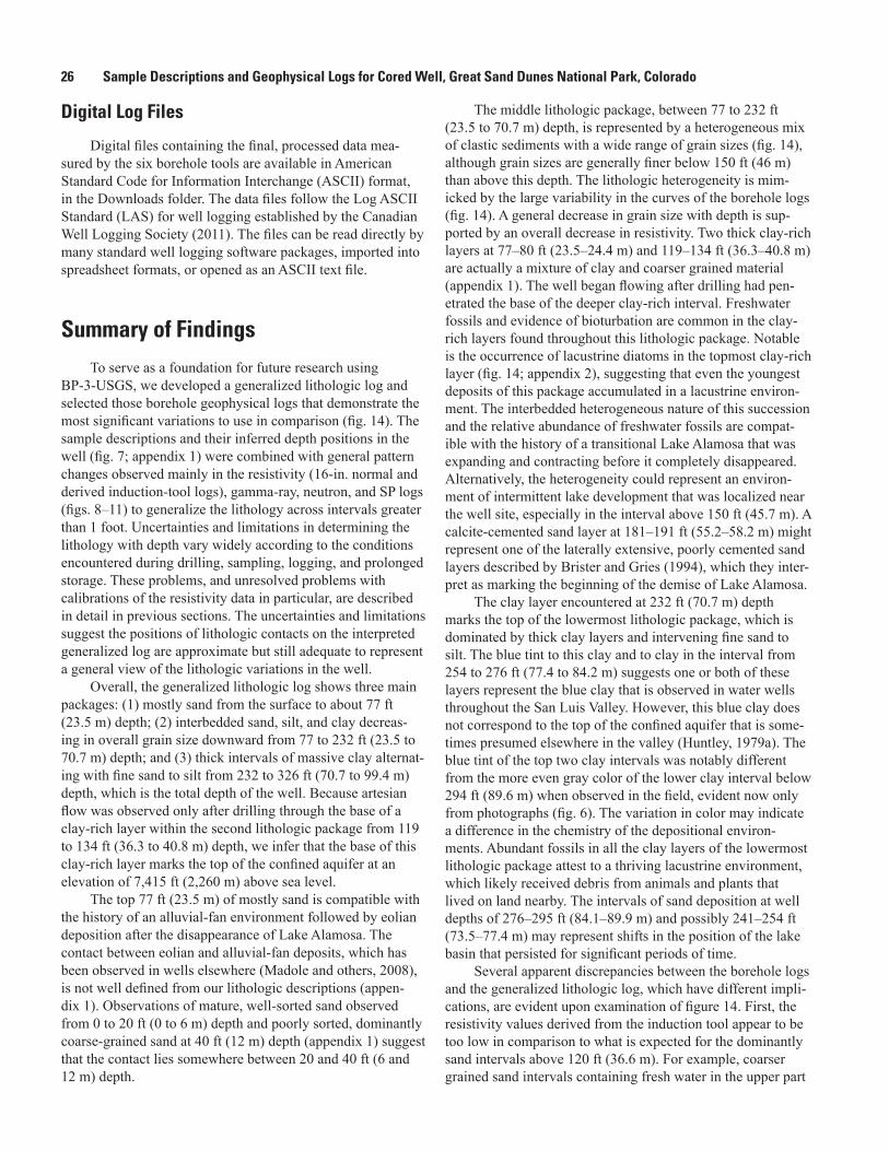
26 Sample Descriptions and Geophysical Logs for Cored Well, Great Sand Dunes National Park, Colorado
Digital Log Files
Digital files containing the final, processed data mea-sured by the six borehole tools are available in American Standard Code for Information Interchange (ASCII) format, in the Downloads folder. The data files follow the Log ASCII Standard (LAS) for well logging established by the Canadian Well Logging Society (2011). The files can be read directly by many standard well logging software packages, imported into spreadsheet formats, or opened as an ASCII text file.
Summary of FindingsTo serve as a foundation for future research using
BP-3-USGS, we developed a generalized lithologic log and selected those borehole geophysical logs that demonstrate the most significant variations to use in comparison (fig. 14). The sample descriptions and their inferred depth positions in the well (fig. 7; appendix 1) were combined with general pattern changes observed mainly in the resistivity (16-in. normal and derived induction-tool logs), gamma-ray, neutron, and SP logs (figs. 8–11) to generalize the lithology across intervals greater than 1 foot. Uncertainties and limitations in determining the lithology with depth vary widely according to the conditions encountered during drilling, sampling, logging, and prolonged storage. These problems, and unresolved problems with calibrations of the resistivity data in particular, are described in detail in previous sections. The uncertainties and limitations suggest the positions of lithologic contacts on the interpreted generalized log are approximate but still adequate to represent a general view of the lithologic variations in the well.
Overall, the generalized lithologic log shows three main packages: (1) mostly sand from the surface to about 77 ft (23.5 m) depth; (2) interbedded sand, silt, and clay decreas-ing in overall grain size downward from 77 to 232 ft (23.5 to 70.7 m) depth; and (3) thick intervals of massive clay alternat-ing with fine sand to silt from 232 to 326 ft (70.7 to 99.4 m) depth, which is the total depth of the well. Because artesian flow was observed only after drilling through the base of a clay-rich layer within the second lithologic package from 119 to 134 ft (36.3 to 40.8 m) depth, we infer that the base of this clay-rich layer marks the top of the confined aquifer at an elevation of 7,415 ft (2,260 m) above sea level.
The top 77 ft (23.5 m) of mostly sand is compatible with the history of an alluvial-fan environment followed by eolian deposition after the disappearance of Lake Alamosa. The contact between eolian and alluvial-fan deposits, which has been observed in wells elsewhere (Madole and others, 2008), is not well defined from our lithologic descriptions (appen-dix 1). Observations of mature, well-sorted sand observed from 0 to 20 ft (0 to 6 m) depth and poorly sorted, dominantly coarse-grained sand at 40 ft (12 m) depth (appendix 1) suggest that the contact lies somewhere between 20 and 40 ft (6 and 12 m) depth.
The middle lithologic package, between 77 to 232 ft (23.5 to 70.7 m) depth, is represented by a heterogeneous mix of clastic sediments with a wide range of grain sizes (fig. 14), although grain sizes are generally finer below 150 ft (46 m) than above this depth. The lithologic heterogeneity is mim-icked by the large variability in the curves of the borehole logs (fig. 14). A general decrease in grain size with depth is sup-ported by an overall decrease in resistivity. Two thick clay-rich layers at 77–80 ft (23.5–24.4 m) and 119–134 ft (36.3–40.8 m) are actually a mixture of clay and coarser grained material (appendix 1). The well began flowing after drilling had pen-etrated the base of the deeper clay-rich interval. Freshwater fossils and evidence of bioturbation are common in the clay-rich layers found throughout this lithologic package. Notable is the occurrence of lacustrine diatoms in the topmost clay-rich layer (fig. 14; appendix 2), suggesting that even the youngest deposits of this package accumulated in a lacustrine environ-ment. The interbedded heterogeneous nature of this succession and the relative abundance of freshwater fossils are compat-ible with the history of a transitional Lake Alamosa that was expanding and contracting before it completely disappeared. Alternatively, the heterogeneity could represent an environ-ment of intermittent lake development that was localized near the well site, especially in the interval above 150 ft (45.7 m). A calcite-cemented sand layer at 181–191 ft (55.2–58.2 m) might represent one of the laterally extensive, poorly cemented sand layers described by Brister and Gries (1994), which they inter-pret as marking the beginning of the demise of Lake Alamosa.
The clay layer encountered at 232 ft (70.7 m) depth marks the top of the lowermost lithologic package, which is dominated by thick clay layers and intervening fine sand to silt. The blue tint to this clay and to clay in the interval from 254 to 276 ft (77.4 to 84.2 m) suggests one or both of these layers represent the blue clay that is observed in water wells throughout the San Luis Valley. However, this blue clay does not correspond to the top of the confined aquifer that is some-times presumed elsewhere in the valley (Huntley, 1979a). The blue tint of the top two clay intervals was notably different from the more even gray color of the lower clay interval below 294 ft (89.6 m) when observed in the field, evident now only from photographs (fig. 6). The variation in color may indicate a difference in the chemistry of the depositional environ-ments. Abundant fossils in all the clay layers of the lowermost lithologic package attest to a thriving lacustrine environment, which likely received debris from animals and plants that lived on land nearby. The intervals of sand deposition at well depths of 276–295 ft (84.1–89.9 m) and possibly 241–254 ft (73.5–77.4 m) may represent shifts in the position of the lake basin that persisted for significant periods of time.
Several apparent discrepancies between the borehole logs and the generalized lithologic log, which have different impli-cations, are evident upon examination of figure 14. First, the resistivity values derived from the induction tool appear to be too low in comparison to what is expected for the dominantly sand intervals above 120 ft (36.6 m). For example, coarser grained sand intervals containing fresh water in the upper part
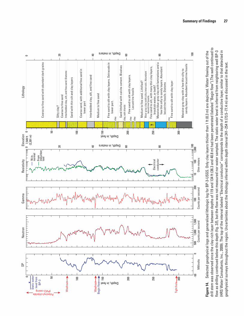
Summary of Findings 27
Figu
re 1
4.
Sele
cted
geo
phys
ical
logs
and
gen
eral
ized
litho
logi
c lo
g fo
r BP-
3-US
GS. O
nly
clay
laye
rs th
icke
r tha
n 1
ft (0
.3 m
) are
dep
icte
d. W
ater
flow
ing
out o
f the
dr
ill s
tem
was
obs
erve
d on
ce th
e cl
ay-r
ich
laye
r bet
wee
n de
pths
of 1
19 a
nd 1
34 ft
(36.
3 an
d 40
.8 m
) had
bee
n pe
netra
ted
(labe
led
“Beg
in fl
ow”)
.The
wel
l con
tinue
d to
flo
w a
s dr
illin
g co
ntin
ued
belo
w th
is d
epth
(fig
. 2E)
, but
the
flow
was
not
mea
sure
d no
r wat
er s
ampl
ed. T
he s
tatic
wat
er le
vel i
s in
ferr
ed fr
om n
eigh
borin
g w
ell B
P-3
(HRS
Wat
er C
onsu
ltant
s, In
c., 2
009)
. The
top
of th
e in
terv
al la
bele
d “E
lect
rical
con
duct
or”
corr
espo
nds
to th
e de
pth
of a
con
duct
ive
laye
r, si
mila
r to
that
det
ecte
d in
ge
ophy
sica
l sur
veys
thro
ugho
ut th
e re
gion
. Unc
erta
intie
s ab
out t
he li
thol
ogy
infe
rred
with
in d
epth
inte
rval
241
–254
ft (7
3.5–
77.4
m) a
re d
iscu
ssed
in th
e te
xt.
1010
01,
000
Resi
stiv
ity
Ohm
-met
ers
From
in
duct
ion
tool
16-in
.no
rmal
0 20 40 60 80 100Depth, in meters
100
200
Gam
ma
Coun
ts p
er s
econ
d50
01,
000
1,50
0
Neu
tron
Coun
ts p
er s
econ
d
SP
-50
0M
illiv
olts
0 50
150
200
250
300
Depth, in feet100
Tigh
t hol
e
Was
hout
Was
hout
Polyvinyl chloride(PVC) casingSt
atic
wat
erle
vel f
rom
BP-3
Begi
n flo
w
clay
clay
, ash
sha
rds
clay
clay
claySa
nd li
thifi
ed w
ith c
alci
te c
emen
t. B
ival
ves
Med
ium
to fi
ne s
and.
Lith
ified
?B
lue-
gray
cla
y w
ith s
ilty
inte
rval
s. A
bund
ant
lacu
stri
ne fo
ssils
Fine
san
d to
silt
, with
man
y th
in c
lay
laye
rs,
brac
kish
wat
er, o
r bot
h?M
assi
ve b
lue-
gray
cla
y w
ith la
min
atio
ns a
nd a
fe
w th
in s
ilty
to s
andy
laye
rs. A
bund
ant
lacu
strin
e fo
ssils
. Dia
tom
s
Fine
san
d to
silt
with
cla
y la
yer
Mas
sive
gra
y cl
ay w
ith a
few
thin
silt
y to
sa
ndy
laye
rs. A
bund
ant l
acus
trin
e fo
ssils
Fine
san
d to
silt
with
cla
y la
yers
. Ost
raco
ds in
lo
wer
par
t.
Fine
san
d to
silt
with
cla
y la
yers
. La
cust
rine
foss
ils
Inte
rbed
ded
clay
, silt
, and
fine
san
d
Silty
cla
y?
Coar
se to
fine
san
d w
ith a
bund
ant d
ark
grai
ns
Coar
se to
fine
san
dIn
terb
edde
d cl
ay, s
ilt, a
nd fi
ne s
and.
Dia
tom
s
Sand
with
thin
silt
and
cla
y la
yers
Med
ium
to fi
ne s
and
Lith
olog
y
?
Coar
se s
and,
with
add
ition
al fi
ne s
and
in
low
er p
art
50 150
200
250
300
100
Depth, in feet
0 20 40 60 80 100Depth, in meters
0El
evat
ion
7,54
9 ft
(2,3
01 m
)
Elec
trica
lco
nduc
tor
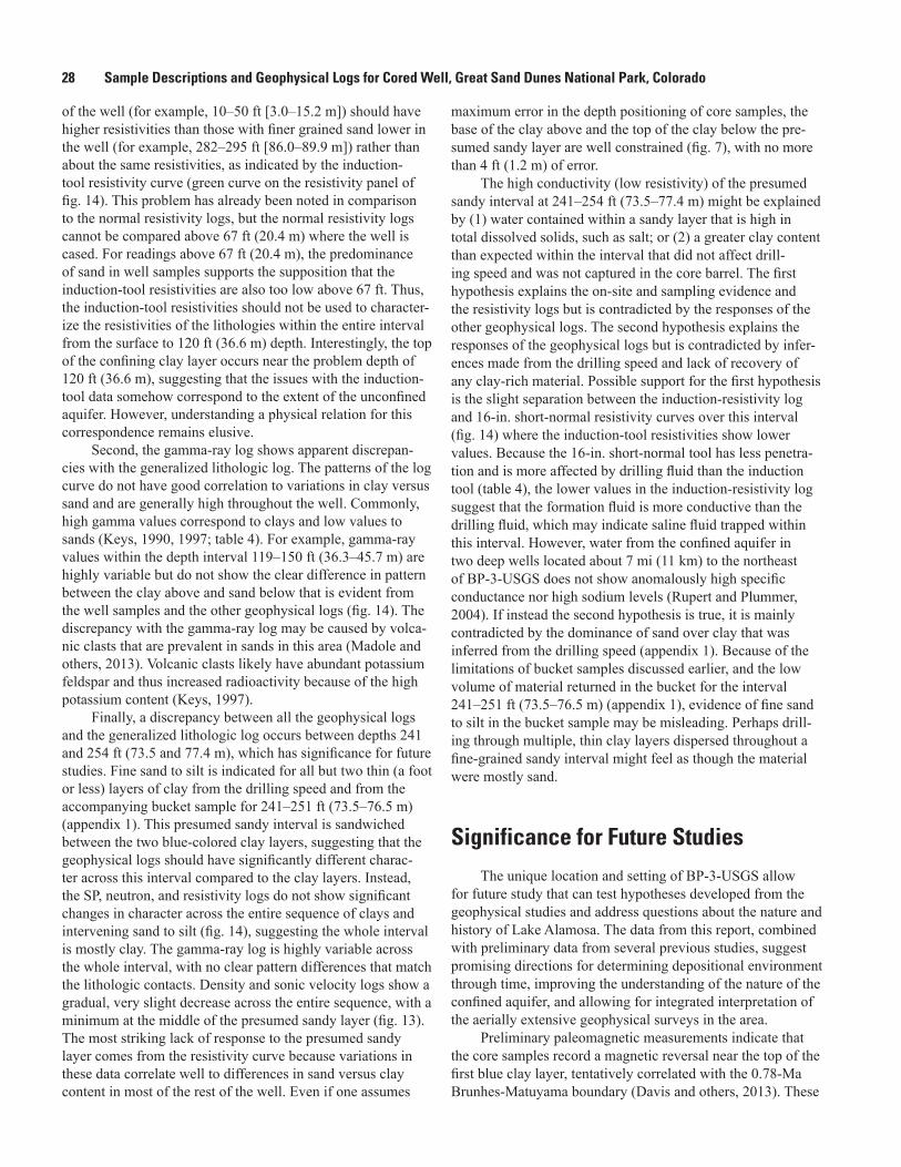
28 Sample Descriptions and Geophysical Logs for Cored Well, Great Sand Dunes National Park, Colorado
of the well (for example, 10–50 ft [3.0–15.2 m]) should have higher resistivities than those with finer grained sand lower in the well (for example, 282–295 ft [86.0–89.9 m]) rather than about the same resistivities, as indicated by the induction-tool resistivity curve (green curve on the resistivity panel of fig. 14). This problem has already been noted in comparison to the normal resistivity logs, but the normal resistivity logs cannot be compared above 67 ft (20.4 m) where the well is cased. For readings above 67 ft (20.4 m), the predominance of sand in well samples supports the supposition that the induction-tool resistivities are also too low above 67 ft. Thus, the induction-tool resistivities should not be used to character-ize the resistivities of the lithologies within the entire interval from the surface to 120 ft (36.6 m) depth. Interestingly, the top of the confining clay layer occurs near the problem depth of 120 ft (36.6 m), suggesting that the issues with the induction-tool data somehow correspond to the extent of the unconfined aquifer. However, understanding a physical relation for this correspondence remains elusive.
Second, the gamma-ray log shows apparent discrepan-cies with the generalized lithologic log. The patterns of the log curve do not have good correlation to variations in clay versus sand and are generally high throughout the well. Commonly, high gamma values correspond to clays and low values to sands (Keys, 1990, 1997; table 4). For example, gamma-ray values within the depth interval 119–150 ft (36.3–45.7 m) are highly variable but do not show the clear difference in pattern between the clay above and sand below that is evident from the well samples and the other geophysical logs (fig. 14). The discrepancy with the gamma-ray log may be caused by volca-nic clasts that are prevalent in sands in this area (Madole and others, 2013). Volcanic clasts likely have abundant potassium feldspar and thus increased radioactivity because of the high potassium content (Keys, 1997).
Finally, a discrepancy between all the geophysical logs and the generalized lithologic log occurs between depths 241 and 254 ft (73.5 and 77.4 m), which has significance for future studies. Fine sand to silt is indicated for all but two thin (a foot or less) layers of clay from the drilling speed and from the accompanying bucket sample for 241–251 ft (73.5–76.5 m) (appendix 1). This presumed sandy interval is sandwiched between the two blue-colored clay layers, suggesting that the geophysical logs should have significantly different charac-ter across this interval compared to the clay layers. Instead, the SP, neutron, and resistivity logs do not show significant changes in character across the entire sequence of clays and intervening sand to silt (fig. 14), suggesting the whole interval is mostly clay. The gamma-ray log is highly variable across the whole interval, with no clear pattern differences that match the lithologic contacts. Density and sonic velocity logs show a gradual, very slight decrease across the entire sequence, with a minimum at the middle of the presumed sandy layer (fig. 13). The most striking lack of response to the presumed sandy layer comes from the resistivity curve because variations in these data correlate well to differences in sand versus clay content in most of the rest of the well. Even if one assumes
maximum error in the depth positioning of core samples, the base of the clay above and the top of the clay below the pre-sumed sandy layer are well constrained (fig. 7), with no more than 4 ft (1.2 m) of error.
The high conductivity (low resistivity) of the presumed sandy interval at 241–254 ft (73.5–77.4 m) might be explained by (1) water contained within a sandy layer that is high in total dissolved solids, such as salt; or (2) a greater clay content than expected within the interval that did not affect drill-ing speed and was not captured in the core barrel. The first hypothesis explains the on-site and sampling evidence and the resistivity logs but is contradicted by the responses of the other geophysical logs. The second hypothesis explains the responses of the geophysical logs but is contradicted by infer-ences made from the drilling speed and lack of recovery of any clay-rich material. Possible support for the first hypothesis is the slight separation between the induction-resistivity log and 16-in. short-normal resistivity curves over this interval (fig. 14) where the induction-tool resistivities show lower values. Because the 16-in. short-normal tool has less penetra-tion and is more affected by drilling fluid than the induction tool (table 4), the lower values in the induction-resistivity log suggest that the formation fluid is more conductive than the drilling fluid, which may indicate saline fluid trapped within this interval. However, water from the confined aquifer in two deep wells located about 7 mi (11 km) to the northeast of BP-3-USGS does not show anomalously high specific conductance nor high sodium levels (Rupert and Plummer, 2004). If instead the second hypothesis is true, it is mainly contradicted by the dominance of sand over clay that was inferred from the drilling speed (appendix 1). Because of the limitations of bucket samples discussed earlier, and the low volume of material returned in the bucket for the interval 241–251 ft (73.5–76.5 m) (appendix 1), evidence of fine sand to silt in the bucket sample may be misleading. Perhaps drill-ing through multiple, thin clay layers dispersed throughout a fine-grained sandy interval might feel as though the material were mostly sand.
Significance for Future StudiesThe unique location and setting of BP-3-USGS allow
for future study that can test hypotheses developed from the geophysical studies and address questions about the nature and history of Lake Alamosa. The data from this report, combined with preliminary data from several previous studies, suggest promising directions for determining depositional environment through time, improving the understanding of the nature of the confined aquifer, and allowing for integrated interpretation of the aerially extensive geophysical surveys in the area.
Preliminary paleomagnetic measurements indicate that the core samples record a magnetic reversal near the top of the first blue clay layer, tentatively correlated with the 0.78-Ma Brunhes-Matuyama boundary (Davis and others, 2013). These

Significance for Future Studies 29
findings suggest that ages for other intervals of the well can be extrapolated from this interval by determining reasonable sedimentation rates. Volcanic ash shards found in several intervals should be evaluated for age dating or tephrochrono-logic correlation to samples of known age. Obtaining ages at these intervals would better establish the chronology of the well stratigraphy, confirm the paleomagnetic results, and allow correlation with similar results from outcrop and core samples studied at Hansen Bluff, 24 mi (38 km) to the south (fig. 1) (Rogers and others, 1992; Machette and others, 2007).
Once age is estimated, more detailed studies of the samples could yield information about depositional environ-ment through time. The strategic approach of the studies might follow that of the Hansen Bluff studies. Variations noted in species of ostracods, pollen, fish, and vertebrates in these studies indicated periods of warm versus cold climate (Rogers and others, 1992), which have potential for correla-tion with species present within BP-3-USGS. In particular, the warm-climate ostracod species Limnocythere bradburyi makes up a coquina at the base of Hansen Bluff near a layer of Bishop Tuff ash (Rogers and others, 1992), which has an age of 774 kilo-annum (ka) (Sarna-Wojcicki and others, 2000). L. bradburyi was also identified in the blue clay at a depth of 93 m in a deep water well 7 mi (11 km) to the northeast of BP-3-USGS (reported in Madole and others, 2013). If this spe-cies is also identified in the blue clay of BP-3-USGS, deposi-tional environment might be correlated across a wide area. If the timing of these variations in environment can be estimated, the findings will have implications for geologic and climatic history for the San Luis Valley. Correlations with worldwide events and geologic mapping of the Rio Grande rift may lead to conclusions about the role of climate versus tectonics dur-ing geologic history.
Investigations of BP-3-USGS can also test hypotheses about when and how Lake Alamosa dried up after breach-ing its lava dam at about 440 ka (Machette and others, 2013). In question is whether sediments from depths of 77–119 ft (23.5–36.3 m), which lie above the confining clay layer, represent transgressions and regressions of Lake Alamosa or whether they were deposited in a local setting with less sig-nificance, such as a fluvial environment with migrating oxbow lakes. Preliminary examination of diatoms in the shallow clay layer at 77 ft (23.5 m) depth (fig. 14; appendix 2) indi-cates a strong presence of a species resembling Aulacoseira distans that is known to inhabit small, acidic lakes (Florin, 1981; Camburn and Kingston, 1986; Haworth, 1988; Siver and Kling, 1997; Camburn and Charles, 2000). The genus Stephanodiscus was also observed in the clay layer, which is a common planktonic form in lakes, ponds, and large rivers (Stoermer and Julius, 2003). Combined with age estimates, these findings may provide evidence for a revised time frame for the demise of Lake Alamosa.
Diatoms were anticipated in a number of other intervals throughout the core; a few were sampled (appendix 2). One additional interval that yielded diatoms was the blue clay at 261–266 ft (79.6–81.1 m) depth. Preliminary examination
of a sample from this interval revealed not only specimens resembling Aulacoseira distans, but also a species resem-bling Anomoeoneis sphaerophora f. costata that inhabits high-conductance and brackish waters (Kociolek and Spauld-ing, 2003) and is among species that are prevalent in highly alkaline waters (Schmid, 1977). Additional pennate diatoms were also observed. Though appearing contradictory as to the suggested nature of the lake setting, the importance of this find is that one could interpret the specimens of Anomoeoneis as suggestive of a nearby shoreline habitat that had migrated closer to the borehole location due to lake drawdown. Such evidence could have implications for the paleoclimate, the basin geometry, or the regional tectonics. Because no diatoms were discovered in samples from Hansen Bluff (Rogers and others, 1992), the documented presence of diatoms in the BP-3-USGS core presents a unique opportunity for a more systematic diatom study that could assist with future interpre-tations of the lake history.
Although BP-3-USGS was not drilled to investigate hydrology, two results are significant or worth further study. First, establishing the top of the confined aquifer adds valu-able information for regional groundwater models of the area, given the paucity of wells penetrating the confined aquifer in Great Sand Dunes National Park and Preserve (Rupert and Plummer, 2004). Second, the alternate hypotheses to explain the conflict in geophysical log response across the apparent sandy interval at 241–254 ft (73.5–77.4 m) requires further evaluation. Follow-up work would likely focus on additional processing of the geophysical logs and evaluation of other deep wells in the region because core was not recovered from this interval.
Finally, the three general lithologic packages observed in the well have good correspondence to the resistivity model determined from the time-domain EM sounding acquired before drilling (fig. 12). A resistive (>80 ohm-m) layer above 85 ft (25.9 m) depth corresponds well to the upper package of mostly sand, with the uppermost, very resistive 15 ft (4.6 m) perhaps representing unsaturated sand. A 20-ohm-m model layer extending from 85 to 235 ft (25.9 to 71.6 m) corresponds well to the middle interbedded sand, silt, and clay package. Most importantly, the low resistivities (high conductivities) of the lowermost model layer, which is also shown by the resistivity logs (fig. 12), mark the top of the lowermost pack-age containing thick clay layers. Similar model resistivity layers have been observed throughout the park and vicinity in both ground-based and airborne EM surveys (Fitterman and Grauch, 2010; Bedrosian and others, 2012). Most notably, BP-3-USGS supports the hypothesis that the persistent, strong electrical conductor observed in the geophysical surveys corresponds to the top of the first observance of massive blue clay. This confirmation allows future studies to use the electri-cal conductor as a proxy to correlate this regional clay across a much wider area. Moreover, if the low resistivity (high electri-cal conductivity) of the sandy interval between the two blue clay layers in BP-3-USGS is caused by saline water, locating the electrical conductor from geophysical surveys may also

30 Sample Descriptions and Geophysical Logs for Cored Well, Great Sand Dunes National Park, Colorado
locate this unusual layer elsewhere, where its nature can be tested.
Acknowledgments
We thank the USGS Central Region drilling and logging team (Art Clarke, Jeff Eman, Steve Grant, Mike Williams, Derek Gongaware, and Barbara Corland) for their expertise, good humor, and invaluable help. We are indebted to Harland Goldstein (USGS) for his critical support in the sampling operations and field work. We thank Andrew Valdez (NPS) and Fred Bunch (NPS) for their help and advice at the drill site. Invaluable assistance was provided by USGS scientists Janet Slate and Mark Hudson in preliminary evaluations of the well samples and Phil Nelson, Bruce Smith, and especially Greg Stanton, in processing the geophysical logs. We are grateful to HRS Water Consultants, who generously provided advice and information. We appreciate the logistical support and collaboration of the Water Resources Division of NPS, in particular, Jim Harte. Finally, we appreciate the funding and moral support for this serendipitous endeavor by the National Cooperative Geologic Mapping Program, especially Randy Orndorff (USGS).
References Cited
Bedrosian, P.A., Grauch, V.J.S., Bloss, B.R., Fitterman, D.V., Abraham, J.D., and Drenth, B.J., 2012, Mapping lacustrine deposits and faults within the east-central San Luis Basin, Rio Grande rift, using airborne electromagnetic surveys [abs.]: Geological Society of America Abstracts with Pro-grams, v. 44, no. 6, p. 79.
Brendle, D.L., 2002, Geophysical logging to determine con-struction, contributing zones, and appropriate use of water levels measured in confined-aquifer network wells, San Luis Valley, Colorado, 1998–2000: U.S. Geological Survey Water-Resources Investigations Report 02–4058, 58 p.
Brister, B.S., and Gries, R.R., 1994, Tertiary stratigraphy and tectonic development of the Alamosa basin (northern San Luis Basin), Rio Grande rift, south-central Colorado, in Keller, G.R., and Cather, S.M., eds., Basins of the Rio Grande rift—Structure, stratigraphy, and tectonic setting: Geological Society of America Special Paper 291, p. 39–58.
Burke, L., 2011, Digital signal processing and interpretation of full waveform sonic log for well BP-3-USGS, Great Sand Dunes National Park and Preserve, Alamosa County, Colorado: U.S. Geological Survey Scientific Investigations Report 2010–5258, 4 p.
Camburn, K.E., and Charles, D.F., 2000, Diatoms of low-alka-linity lakes in the northeastern United States: The Academy of Natural Sciences of Philadelphia Special Publication 18, 152 p.
Camburn, K.E., and Kingston, J.C., 1986, The genus Melosira from soft-water lakes with special reference to northern Michigan, Wisconsin and Minnesota, in Smol, J.P., Battar-bee, R.W., Davis, R.B., and Meriläinen, J.A., eds., Diatoms and lake acidity—Reconstructing pH from siliceous algal remains in lake sediments: Springer-Verlag, Developments in Hydrobiology no. 29, p. 17–34.
Canadian Well Logging Society, 2011, LAS information—Log ASCII Standard (LAS) software: Canadian Well Logging Society Web site, accessed August 19, 2014, at http://www.cwls.org/las/.
Colman, S.M., McCalpin, J.P., Ostenaa, D.A., and Kirkham, R.M., 1985, Map showing upper Cenozoic rocks and depos-its and Quaternary faults, Rio Grande rift, south-central Colorado: U.S. Geological Survey Miscellaneous Investiga-tions Map I–1594, 2 sheets, scale 1:125,000.
Davis, J.K., Hudson, M.R., Slate, J.L., and Grauch, V.J.S., 2013, Preliminary magnetic analysis of the USGS BP3 core, Great Sand Dunes National Park, Colorado [abs.]: Geo-logical Society of America Abstracts with Programs, v. 45, no. 7, p. 603.
Emery, P.A., Snipes, R.J., Dumeyer, J.M., and Klein, J.M., 1973, Water in the San Luis Valley, south-central Colorado: Colorado Water Resources Circular 18, 26 p., 10 pls.
Fitterman, D.V., and de Souza Filho, O.A., 2009, Tran-sient electromagnetic soundings near Great Sand Dunes National Park and Preserve, San Luis Valley, Colorado (2006 field season): U.S. Geological Survey Open-File Report 2009–1051, 55 p.
Fitterman, D.V., and Grauch, V.J.S., 2010, Transient electro-magnetic mapping of clay units in the San Luis Valley, Col-orado: Proceedings of the 23rd Symposium on the Appli-cation of Geophysics to Engineering and Environmental Problems (SAGEEP), 2010 Environmental & Engineering Geophysical Society (EEGS) Annual Meeting, April 11–15, 2010, p. 154–164.
Fitterman, D.V., and Labson, V.F., 2005, Electromagnetic induction methods for environmental problems, in Butler, D.K., ed., Near surface geophysics, part 1—Concepts and fundamentals: Tulsa, Okla., Society of Exploration Geo-physicists, p. 301–355.
Florin, M.-B., 1981, The taxonomy of some Melosira spe-cies—A comparative morphological study, in Ross, R., ed.: II. Proceedings of the 6th International Sympo-sium on Recent and Fossil Marine Diatoms, Budapest, September 1–5, 1980, p. 43–67.

References Cited 31
Fraser, D.C., Fuller, B.D., and Ward, S.H., 1966, Some numerical techniques for application in mining exploration: Geophysics, v. 31, no. 6, p. 1066–1077.
Gardner, G.H.F., Gardner, L.W., and Gregory, A.R., 1974, Formation velocity and density—The diagnostic basics for stratigraphic traps: Geophysics, v. 39, no. 6, p. 770–780.
Grauch, V.J.S., Bedrosian, P.A., Drenth, B.J., and Bloss, B.R., 2013, Mapping under the sand—Progress report on geophysical studies in Great Sand Dunes National Park, Colorado [abs.]: Geological Society of America Abstracts with Programs, v. 45, no. 7, p. 67.
Grauch, V.J.S., Fitterman, D.V., Slate, J.L., and Drenth, B.J., 2010, Mapping Plio-Pleistocene lake deposits under Great Sand Dunes National Park, San Luis Valley, Colorado—Insights from recent drilling and geophysical surveys [abs.]: Geological Society of America Abstracts with Programs, v. 42, no. 5, p. 455.
Harmon, E.J., 2010, Hydrogeologic controls by depositional and lithofacies transitions—Great Sand Dunes National Park and Preserve, Colorado [abs.]: Geological Society of America Abstracts with Programs, v. 42, no. 5, p. 454.
Haworth, E.Y., 1988, Distribution of diatom taxa of the old genus Melosira (now mainly Aulacoseira) in Cumbrian waters, in Round, E.F., ed., Algae and the aquatic environ-ment: Bristol, United Kingdom, Biopress, p. 138–167.
Hearne, G.A., and Dewey, J.D., 1988, Hydrologic analysis of the Rio Grande Basin north of Embudo, New Mexico, Colorado and New Mexico: U.S. Geological Survey Water-Resources Investigations Report 86–4113, 244 p., 1 pl.
HRS Water Consultants, Inc., 1999, Hydrogeologic investiga-tion, Sand Creek and Indian Springs area, Great Sand Dunes National Monument, Colorado: Lakewood, Colo., HRS Water Consultants, Inc., Report to National Park Service 92021–04, 40 p.
HRS Water Consultants, Inc., 2009, Documentation of bound-ary piezometer installation, Great Sand Dunes National Park and Preserve, Colorado: Lakewood, Colo., HRS Water Consultants, Inc., Report to U.S. Department of Justice and National Park Service, December 2009, HRS Project 04-06.10.
Huntley, David, 1979a, Ground-water recharge to the aquifers of northern San Luis Valley, Colorado: Geological Society of America Bulletin, Part II, v. 90, no. 8, p. 1196–1281.
Huntley, David, 1979b, Cenozoic faulting and sedimentation in northern San Luis Valley, Colorado: Geological Society of America Bulletin, Part II, v. 90, no. 1, p. 135–153.
Keys, W.S., 1990, Borehole geophysics applied to ground-water investigations: U.S. Geological Survey Techniques of Water Resources Investigations Book 2, chapter E–2, 150 p.
Keys, W.S., 1997, A practical guide to borehole geophysics in environmental investigations: Boca Raton, Fla., CRC-Lewis Publishers, 176 p.
Kirkham, R.M., and Rogers, W.P., 1981, Earthquake poten-tial in Colorado: Colorado Geological Survey Bulletin 43, p. 171.
Knight, R.J., and Endres, A.L., 2005, An introduction to rock physics principles for near-surface geophysics, in Butler, D.K., ed., Near surface geophysics, part 1—Concepts and fundamentals: Tulsa, Okla., Society of Exploration Geo-physicists, p. 31–70.
Kociolek, J.P., and Spaulding, S.A., 2003, Symmetrical Naviculoid diatoms, in Wehr, J.D., and Sheath, R.G., eds., Freshwater algae of North America—Ecology and classifi-cation: New York, Academic Press, p. 637–668.
Machette, M.N., 2007, Chapter B—Field trip day 2—Qua-ternary geology of Lake Alamosa and the Costilla Plain, southern Colorado, in Machette, M.N., Coates, M.-M., and Johnson, M.L., eds., 2007 Rocky Mountain Section Friends of the Pleistocene Field Trip—Quaternary geology of the San Luis Basin of Colorado and New Mexico, Septem-ber 7–9, 2007: U.S. Geological Survey Open-File Report 2007–1193, p. 53–108. http://pubs.usgs.gov/of/2007/1193/.
Machette, M.N., Marchetti, D.W., and Thompson, R.A., 2007, Chapter G—Ancient Lake Alamosa and the Plio-cene to middle Pleistocene evolution of the Rio Grande, in Machette, M.N., Coates, M.-M., and Johnson, M.L., eds., 2007 Rocky Mountain Section Friends of the Pleis-tocene Field Trip—Quaternary geology of the San Luis Basin of Colorado and New Mexico, September 7–9, 2007: U.S. Geological Survey Open-File Report 2007–1193, p. 157–167, http://pubs.usgs.gov/of/2007/1193/.
Machette, M.N., Thompson, R.A., Marchetti, D.W., and Smith, R.S.U., 2013, Evolution of ancient Lake Alamosa and integration of the Rio Grande during the Pliocene and Pleistocene, in Hudson, M.R., and Grauch, V.J.S., eds., New perspectives on Rio Grande rift basins—From tectonics to groundwater: Geological Society of America Special Paper 494, p. 1–20.
Madole, R.F., Mahan, S.A., Romig, J.H., and Havens, J.C., 2013, Constraints on the age of the Great Sand Dunes, Colorado, from subsurface stratigraphy and OSL dates: Quaternary Research, v. 80, p. 435–446.
Madole, R.F., Romig, J.H., Aleinikoff, J.N., VanSistine, D.P., and Yacob, E.Y., 2008, On the origin and age of the Great Sand Dunes, Colorado: Geomorphology, v. 99, p. 99–119.
Naudy H., and Dreyer H., 1968, Essai de filtrage nonlineare applique aux profils aeromagnetiques: Geophysical Pros-pecting, v. 16, no. 2, p. 171.

32 Sample Descriptions and Geophysical Logs for Cored Well, Great Sand Dunes National Park, Colorado
Rogers, K.L., Larson, E.E., Smith, G., Katzman, D., Smith, G.R., Cerling, T., Wang, Y., Baker, R.G., Lohmann, K.C., Repenning, C.A., Patterson, P., and Mackie, G., 1992, Plio-cene and Pleistocene geologic and climatic evolution in the San Luis Valley of south-central Colorado: Palaeogeogra-phy, Palaeoclimatology, Palaeoecology, v. 94, p. 55–86.
Rogers, K.L., Repenning, C.A., Forester, R.M., Larson, E.E., Hall, S.A., Smith, G.R., Anderson, E., and Brown, T.J., 1985, Middle Pleistocene (late Irvingtonian: Nebrasakan) climatic changes in south-central Colorado: National Geo-graphic Research, v. 1, no. 4, p. 535–563.
Ruleman, C., and Machette, M.N., 2007, An overview of the Sangre de Cristo fault system and new insights to interac-tions between Quaternary faults in the northern Rio Grande rift, in Machette, M.N., Coates, M.-M., and Johnson, M.L., eds., 2007 Rocky Mountain Section Friends of the Pleistocene field trip–Quaternary geology of the San Luis Basin of Colorado and New Mexico, September 7–9, 2007: U.S. Geological Survey Open-File Report 2007–1193, p. 187–197.
Rupert, M.G., and Plummer, L.N., 2004, Ground-water flow direction, water quality, recharge sources, and age, Great Sand Dunes National Monument, south-central Colorado, 2000–2001: U.S. Geological Survey Scientific Investiga-tions Report 2004–5027, 28 p.
Sarna-Wojcicki, A.M., Pringle, M.S., Wijbrans, J., 2000, New 40Ar/39Ar age of the Bishop Tuff from multiple sites and sediment rate calibration for the Matuyama-Brunhes boundary: Journal of Geophysical Research, v. 105, no. B9, p. 21,431–21,443.
Schmid, A., 1977, Morphological and physiological examina-tion of diatoms of Neusiedler Lake. 2. Photomicroscopic and scanning electron-microscopic shell analysis of envi-ronmentally conditioned cyclomorphosis of Anomoeoneis-sphaerophora (KG) Pfitzer: Nova Hedwigia, v. 28, no. 2-3, p. 309–351.
Scott, J.H., 1978, A FORTRAN algorithm for correcting nor-mal resistivity logs for borehole diameter and mud resistiv-ity: U.S. Geological Survey Open-File Report 78–669, 12 p.
Siebenthal, C.E., 1910, Geology and water resources of the San Luis Valley, Colorado: U.S. Geological Survey Water Supply Paper 240, 128 p.
Siver, P.A., and Kling, H., 1997, Morphological observations of Aulacoseira using scanning electron microscopy: Cana-dian Journal of Botany, v. 75, p. 1807–1835.
Stoermer, E.F., and Julius, M.L., 2003, Centric diatoms, in Wehr, J.D., and Sheath, R.G., eds., Freshwater algae of North America—Ecology and classification: New York, Academic Press, p. 559–594.

Appendixes

34 Sample Descriptions and Geophysical Logs for Cored Well, Great Sand Dunes National Park, ColoradoA
ppen
dix
1.
Desc
riptio
ns o
f sam
ples
by
type
and
dril
ling
inte
rval
.
[Dril
ling
dept
h in
terv
al, i
nter
val e
valu
ated
for s
ampl
ing;
thos
e sa
mpl
ed fo
r cor
e ar
e in
dica
ted
by th
e co
re ru
n nu
mbe
r; de
pths
list
ed in
feet
(ft),
cor
resp
ondi
ng to
dril
ling
proc
edur
es; m
, met
ers.
Sam
ple
type
s de
scrib
ed in
text
and
tabl
e 1.
N/A
, not
app
licab
le. X
RD
, X-r
ay d
iffra
ctio
n. A
naly
ses a
re p
rese
nted
in a
ppen
dix
3. O
nsite
cor
e re
cove
ry le
ngth
is th
e or
igin
al le
ngth
mea
sure
d in
200
9. C
ores
are
logg
ed fr
om b
ot-
tom
(0.0
ft) t
o th
e to
p of
the
sam
ple
rela
tive
to c
ore
leng
ths m
easu
red
in 2
013,
whi
ch c
ould
be
diffe
rent
than
the
onsi
te le
ngth
(tab
le 2
). Se
e ap
pend
ix 2
for m
ore
deta
il on
foss
il an
d tra
ce fo
ssil
obse
rvat
ions
.]
Dri
lling
dep
th
inte
rval
Des
crip
tion
from
dri
lling
spe
ed
and
onsi
te o
bser
vatio
nsD
escr
iptio
ns o
f mud
str
eam
sam
ples
Des
crip
tions
of c
ore
barr
el s
ampl
es
0–20
ft(0
–6.1
m)
Rot
ary
drill
ing
Coa
rse
sand
with
clu
mps
of
silty
cla
ySi
eved
cut
tings
at 1
0 ft.
C
oars
e sa
nd to
cla
y w
ith p
oorly
sorte
d su
brou
nded
to
ro
unde
d, m
ostly
dar
k gr
ains
. Slig
htly
cal
care
ous.
Siev
ed c
uttin
gs a
t 20
ft.
Coa
rse
to fi
ne sa
nd w
ith ro
unde
d to
subr
ound
ed g
rain
s.
N
onca
lcar
eous
. H
oppe
r sam
ples
(coa
rse
and
fine
frac
tions
) fro
m 0
–20
ft.
Coa
rse
to v
ery
fine
sand
with
subr
ound
ed to
roun
ded,
mos
tly
da
rk g
rain
s. A
bout
twic
e th
e vo
lum
e of
coa
rse-
com
pare
d
to
fine
-gra
ined
frac
tion.
Ver
y m
atur
e. S
light
ly c
alca
reou
s.
N/A
20–4
0 ft
(6.1
–12.
2 m
)R
otar
y dr
illin
g
Coa
rse
sand
with
clu
mps
of
gre
en c
lay
grad
ing
dow
nwar
d to
fine
sand
Hop
per s
ampl
es (c
oars
e an
d fin
e fr
actio
ns) f
rom
20–
30 ft
. C
oars
e to
fine
sand
with
roun
ded
to su
brou
nded
, mos
tly d
ark
gr
ains
. Non
calc
areo
us.
Siev
ed c
uttin
gs a
t 30
ft.
Coa
rse
to fi
ne sa
nd w
ith ro
unde
d to
subr
ound
ed, m
ostly
dar
k
grai
ns. N
onca
lcar
eous
. H
oppe
r sam
ples
(coa
rse
and
fine
frac
tions
) fro
m 3
0–40
ft.
Coa
rse
to fi
ne sa
nd w
ith su
bang
ular
to ro
unde
d, m
ostly
dar
k
gr
ains
. Non
calc
areo
us. S
ampl
e ta
ken
from
fine
frac
tion
for
X
RD
ana
lysi
sSi
eved
cut
tings
at 4
0 ft.
Ve
ry c
oars
e to
fine
sand
, dom
inat
ed b
y co
arse
sand
. Poo
rly
so
rted,
suba
ngul
ar to
roun
ded,
mos
tly d
ark
grai
ns, s
ome
volc
anic
gra
ins.
Non
calc
areo
us.
N/A
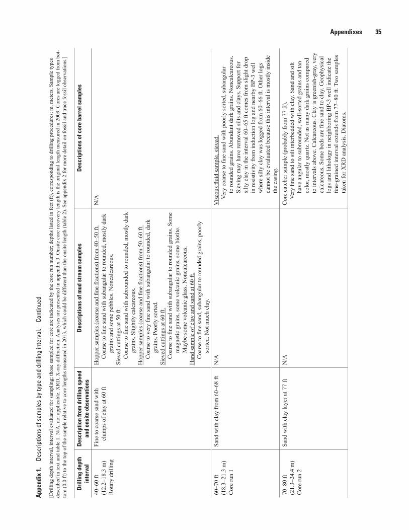
Appendixes 35
Dri
lling
dep
th
inte
rval
Des
crip
tion
from
dri
lling
spe
ed
and
onsi
te o
bser
vatio
nsD
escr
iptio
ns o
f mud
str
eam
sam
ples
Des
crip
tions
of c
ore
barr
el s
ampl
es
40–6
0 ft
(12.
2–18
.3 m
)R
otar
y dr
illin
g
Fine
to c
oars
e sa
nd w
ith
clum
ps o
f cla
y at
60
ftH
oppe
r sam
ples
(coa
rse
and
fine
frac
tions
) fro
m 4
0–50
ft.
Coa
rse
to fi
ne sa
nd w
ith su
bang
ular
to ro
unde
d, m
ostly
dar
k
gr
ains
and
som
e pe
bble
s. N
onca
lcar
eous
.Si
eved
cut
tings
at 5
0 ft.
C
oars
e to
fine
sand
with
subr
ound
ed to
roun
ded,
mos
tly d
ark
gr
ains
. Slig
htly
cal
care
ous.
Hop
per s
ampl
es (c
oars
e an
d fin
e fr
actio
ns) f
rom
50–
60 ft
. C
oars
e to
ver
y fin
e sa
nd w
ith su
bang
ular
to ro
unde
d, d
ark
grai
ns. P
oorly
sorte
d.Si
eved
cut
tings
at 6
0 ft.
C
oars
e to
fine
sand
with
suba
ngul
ar to
roun
ded
grai
ns. S
ome
m
agne
tic g
rain
s, so
me
volc
anic
gra
ins,
som
e bi
otite
.
May
be so
me
volc
anic
gla
ss. N
onca
lcar
eous
.H
and
sam
ple
of c
lay
and
sand
at 6
0 ft.
C
oars
e to
fine
sand
, sub
angu
lar t
o ro
unde
d gr
ains
, poo
rly
so
rted.
Not
muc
h cl
ay.
N/A
60–7
0 ft
(18.
3–21
.3 m
)C
ore
run
1
Sand
with
cla
y fr
om 6
0–68
ftN
/A
Vis
cous
flui
d sa
mpl
e, si
eved
. Ve
ry c
oars
e to
fine
sand
with
poo
rly so
rted,
suba
ngul
ar
to
roun
ded
grai
ns. A
bund
ant d
ark
grai
ns. N
onca
lcar
eous
.
Siev
ing
may
hav
e re
mov
ed si
lts a
nd c
lays
. Sup
port
for
si
lty c
lay
in th
e in
terv
al 6
0–65
ft c
omes
from
slig
ht d
rop
in re
sist
ivity
from
indu
ctio
n lo
g an
d ne
arby
BP-
3 w
ell
w
here
silty
cla
y w
as lo
gged
from
60–
66 ft
. Oth
er lo
gs
ca
nnot
be
eval
uate
d be
caus
e th
is in
terv
al is
mos
tly in
side
the
casi
ng.
70–8
0 ft
(21.
3–24
.4 m
)C
ore
run
2
Sand
with
cla
y la
yer a
t 77
ftN
/AC
ore
catc
her s
ampl
e (p
roba
bly
from
77
ft).
Ve
ry fi
ne sa
nd to
silt
inte
rbed
ded
with
cla
y. S
and
and
silt
have
ang
ular
to su
brou
nded
, wel
l-sor
ted
grai
ns a
nd ta
n
co
lor,
mos
tly q
uartz
. Not
as m
any
dark
gra
ins c
ompa
red
to in
terv
als a
bove
. Cal
care
ous.
Cla
y is
gre
enis
h-gr
ay, v
ery
calc
areo
us. S
ome
beds
are
fine
sand
to c
lay.
Geo
phys
ical
logs
and
lith
olog
y in
nei
ghbo
ring
BP-
3 w
ell i
ndic
ate
the
fine-
grai
ned
inte
rval
ext
ends
from
77–
80 ft
. Tw
o sa
mpl
es
ta
ken
for X
RD
ana
lysi
s. D
iato
ms.
App
endi
x 1.
De
scrip
tions
of s
ampl
es b
y ty
pe a
nd d
rillin
g in
terv
al.—
Cont
inue
d
[Dril
ling
dept
h in
terv
al, i
nter
val e
valu
ated
for s
ampl
ing;
thos
e sa
mpl
ed fo
r cor
e ar
e in
dica
ted
by th
e co
re ru
n nu
mbe
r; de
pths
list
ed in
feet
(ft),
cor
resp
ondi
ng to
dril
ling
proc
edur
es; m
, met
ers.
Sam
ple
type
s de
scrib
ed in
text
and
tabl
e 1.
N/A
, not
app
licab
le. X
RD
, X-r
ay d
iffra
ctio
n. A
naly
ses a
re p
rese
nted
in a
ppen
dix
3. O
nsite
cor
e re
cove
ry le
ngth
is th
e or
igin
al le
ngth
mea
sure
d in
200
9. C
ores
are
logg
ed fr
om b
ot-
tom
(0.0
ft) t
o th
e to
p of
the
sam
ple
rela
tive
to c
ore
leng
ths m
easu
red
in 2
013,
whi
ch c
ould
be
diffe
rent
than
the
onsi
te le
ngth
(tab
le 2
). Se
e ap
pend
ix 2
for m
ore
deta
il on
foss
il an
d tra
ce fo
ssil
obse
rvat
ions
.]

36 Sample Descriptions and Geophysical Logs for Cored Well, Great Sand Dunes National Park, Colorado
Dri
lling
dep
th
inte
rval
Des
crip
tion
from
dri
lling
spe
ed
and
onsi
te o
bser
vatio
nsD
escr
iptio
ns o
f mud
str
eam
sam
ples
Des
crip
tions
of c
ore
barr
el s
ampl
es
80–9
0 ft
(24.
4–27
.4 m
)C
ore
run
3
Coa
rse
sand
with
a li
ttle
hard
, da
rk c
lay
N/A
Cor
e ca
tche
r sam
ple
(pos
sibl
y fr
om 8
5 ft,
bas
ed o
n ge
ophy
sica
l lo
gs).
Ve
ry fi
ne sa
nd to
cla
y, m
ostly
silt
with
ver
y lit
tle c
oars
e sa
nd.
W
ell-s
orte
d an
gula
r to
suba
ngul
ar g
rain
s. Fe
wer
dar
k
gr
ains
than
abo
ve, s
ome
mic
a. N
onca
lcar
eous
. Sam
ple
take
n fo
r XR
D a
naly
sis.
90–9
2 ft
(27.
4–28
.0 m
)C
ore
run
4
Dar
k-gr
ay si
lty c
lay
and
fine
sa
nd w
ith la
yer-l
ike
chun
ks
of li
me-
gree
n cl
ay
Siev
e sa
mpl
e at
92
ft.
Coa
rse
to fi
ne sa
nd, a
ngul
ar to
roun
ded
grai
ns, p
oorly
sorte
d.
So
me
mic
a, o
ne la
rge
pota
ssiu
m fe
ldsp
ar g
rain
. Ver
y
ca
lcar
eous
.
Cor
e ca
tche
r plu
s vis
cous
flui
d sa
mpl
es, s
ieve
d.
Very
fine
sand
to si
lt, so
me
coar
se sa
nd, n
ot m
uch
clay
, if
an
y. M
ostly
qua
rtz. L
ots o
f mic
a. M
ediu
m to
wel
l sor
ted.
Slig
htly
cal
care
ous.
92–9
4 ft
(28.
0–28
.7 m
)C
ore
run
5
Sand
with
laye
r-lik
e ch
unks
of
gree
n cl
ayN
/AV
isco
us fl
uid
sam
ple,
scoo
ped.
M
ediu
m to
ver
y fin
e sa
nd, s
uban
gula
r to
roun
ded
grai
ns.
So
me
clum
ps o
f blu
e cl
ay. M
ediu
m so
rting
. Slig
htly
calc
areo
us.
Cor
e ca
tche
r sam
ple.
C
oars
e sa
nd to
silt,
poo
rly so
rted.
Mos
tly q
uartz
gra
ins w
ith
so
me
pota
ssiu
m fe
ldsp
ar, r
elat
ivel
y fe
w d
ark
grai
ns, s
ome
m
agne
tite
grai
ns. V
ery
calc
areo
us.
94–9
6 ft
(28.
7–29
.3 m
)C
ore
run
6
Cla
y ab
ove
med
ium
, dar
k gr
ay
sand
N/A
Cor
e ca
tche
r sam
ple
(pro
babl
y fr
om 9
4 ft)
. Fi
ne sa
nd to
cla
y w
ith w
ell-s
orte
d, a
ngul
ar to
subr
ound
ed
gr
ains
. Clu
mps
of t
an c
lay.
Som
e cl
umps
of m
ediu
m sa
nd
w
ith d
arke
r gra
ins.
Non
calc
areo
us.
96–1
01 ft
(29.
3–30
.8 m
)C
ore
run
7
Sand
N
/A
Vis
cous
flui
d sa
mpl
e, si
eved
. C
oars
e to
ver
y fin
e sa
nd w
ith m
ediu
m-s
orte
d, su
bang
ular
to
ro
unde
d da
rk g
rain
s. N
onca
lcar
eous
. C
ore
catc
her s
ampl
e (p
roba
bly
from
101
ft).
Fi
ne sa
nd to
silt
with
ver
y w
ell-s
orte
d, su
bang
ular
to ro
unde
d
grai
ns. M
oder
atel
y ab
unda
nt d
ark
grai
ns. N
onca
lcar
eous
.
App
endi
x 1.
De
scrip
tions
of s
ampl
es b
y ty
pe a
nd d
rillin
g in
terv
al.—
Cont
inue
d
[Dril
ling
dept
h in
terv
al, i
nter
val e
valu
ated
for s
ampl
ing;
thos
e sa
mpl
ed fo
r cor
e ar
e in
dica
ted
by th
e co
re ru
n nu
mbe
r; de
pths
list
ed in
feet
(ft),
cor
resp
ondi
ng to
dril
ling
proc
edur
es; m
, met
ers.
Sam
ple
type
s de
scrib
ed in
text
and
tabl
e 1.
N/A
, not
app
licab
le. X
RD
, X-r
ay d
iffra
ctio
n. A
naly
ses a
re p
rese
nted
in a
ppen
dix
3. O
nsite
cor
e re
cove
ry le
ngth
is th
e or
igin
al le
ngth
mea
sure
d in
200
9. C
ores
are
logg
ed fr
om b
ot-
tom
(0.0
ft) t
o th
e to
p of
the
sam
ple
rela
tive
to c
ore
leng
ths m
easu
red
in 2
013,
whi
ch c
ould
be
diffe
rent
than
the
onsi
te le
ngth
(tab
le 2
). Se
e ap
pend
ix 2
for m
ore
deta
il on
foss
il an
d tra
ce fo
ssil
obse
rvat
ions
.]
Appendixes 37
Dri
lling
dep
th
inte
rval
Des
crip
tion
from
dri
lling
spe
ed
and
onsi
te o
bser
vatio
nsD
escr
iptio
ns o
f mud
str
eam
sam
ples
Des
crip
tions
of c
ore
barr
el s
ampl
es
101–
119
ft(3
0.8–
36.3
m)
(No
core
sam
ple)
Sand
with
thin
laye
rs o
f cla
y at
11
5 ft
and
119
ftSi
eve
sam
ple
at 1
05 ft
. C
oars
e sa
nd w
ith m
ediu
m-s
orte
d, su
bang
ular
to ro
unde
d
gr
ains
. Abu
ndan
t dar
k gr
ains
. Non
calc
areo
us.
Siev
e sa
mpl
e at
112
ft.
Coa
rse
sand
with
med
ium
-sor
ted,
suba
ngul
ar to
roun
ded
grai
ns. A
bund
ant d
ark
grai
ns. N
onca
lcar
eous
.Si
eve
sam
ple
at 1
15 ft
. C
oars
e sa
nd w
ith m
ediu
m-s
orte
d, su
bang
ular
to ro
unde
d
gr
ains
. Abu
ndan
t dar
k gr
ains
. Non
calc
areo
us.
Siev
e sa
mpl
e at
119
ft.
Coa
rse
to fi
ne sa
nd w
ith p
oorly
sorte
d, su
bang
ular
to ro
unde
d
dark
gra
ins.
Non
calc
areo
us.
N/A
119–
125
ft(3
6.3–
38.1
m)
Cor
e ru
n 8
Cla
y w
ith sa
nd g
radu
ally
in
crea
sing
dow
nwar
d N
/AC
ore
piec
e (1
.6 ft
fell
off c
ore
tabl
e, p
roba
bly
from
119
–121
ft).
Fine
sand
to c
lay
with
suba
ngul
ar to
roun
ded
grai
ns. S
andy
clay
inte
rbed
ded
with
sand
laye
rs. N
onca
lcar
eous
.C
ore
catc
her s
ampl
e.
Fine
sand
to si
lt w
ith w
ell-s
orte
d, a
ngul
ar to
subr
ound
ed
gr
ains
. Mod
erat
ely
abun
dant
dar
k gr
ains
. Non
calc
areo
us,
al
thou
gh li
ght-c
olor
ed p
ocke
ts a
re c
alca
reou
s. Sa
mpl
e
ta
ken
for X
RD
ana
lysi
s.12
5–12
8 ft
(38.
1–39
.0 m
)C
ore
run
9
Cla
yN
/AC
ore
(1.0
ft o
nsite
reco
very
, pro
babl
y fr
om 1
25–1
26 ft
).
0.5–
1.0
Dar
k gr
ay si
lty c
lay
with
few
er d
ark
grai
ns in
the
fine
r mat
eria
l. Sl
ight
ly c
alca
reou
s.
0.0–
0.5
Ligh
t gra
y sa
ndy
clay
. San
d co
nsis
ts o
f abu
ndan
t
dar
k gr
ains
. Slig
htly
cal
care
ous.
Fain
tly b
edde
d.
D
essi
catio
n cr
acks
par
alle
l to
bedd
ing.
Cor
e ca
tche
r sam
ple.
M
ediu
m w
ell s
orte
d si
lt to
cla
y, w
ith v
ery
little
silt.
Som
e m
ica.
Non
calc
areo
us.
128–
131
ft(3
9.0–
39.9
m)
Cor
e ru
n 10
Cla
y ch
angi
ng to
sand
bel
ow
129
ft N
/A
Cor
e ca
tche
r sam
ple
(pro
babl
y fr
om 1
28–1
29 ft
).
Fine
sand
to c
lay,
mos
tly si
lt, w
ith m
ediu
m so
rted,
suba
ngul
ar to
roun
ded
dark
gra
ins.
Very
cal
care
ous.
App
endi
x 1.
De
scrip
tions
of s
ampl
es b
y ty
pe a
nd d
rillin
g in
terv
al.—
Cont
inue
d
[Dril
ling
dept
h in
terv
al, i
nter
val e
valu
ated
for s
ampl
ing;
thos
e sa
mpl
ed fo
r cor
e ar
e in
dica
ted
by th
e co
re ru
n nu
mbe
r; de
pths
list
ed in
feet
(ft),
cor
resp
ondi
ng to
dril
ling
proc
edur
es; m
, met
ers.
Sam
ple
type
s de
scrib
ed in
text
and
tabl
e 1.
N/A
, not
app
licab
le. X
RD
, X-r
ay d
iffra
ctio
n. A
naly
ses a
re p
rese
nted
in a
ppen
dix
3. O
nsite
cor
e re
cove
ry le
ngth
is th
e or
igin
al le
ngth
mea
sure
d in
200
9. C
ores
are
logg
ed fr
om b
ot-
tom
(0.0
ft) t
o th
e to
p of
the
sam
ple
rela
tive
to c
ore
leng
ths m
easu
red
in 2
013,
whi
ch c
ould
be
diffe
rent
than
the
onsi
te le
ngth
(tab
le 2
). Se
e ap
pend
ix 2
for m
ore
deta
il on
foss
il an
d tra
ce fo
ssil
obse
rvat
ions
.]
38 Sample Descriptions and Geophysical Logs for Cored Well, Great Sand Dunes National Park, Colorado
Dri
lling
dep
th
inte
rval
Des
crip
tion
from
dri
lling
spe
ed
and
onsi
te o
bser
vatio
nsD
escr
iptio
ns o
f mud
str
eam
sam
ples
Des
crip
tions
of c
ore
barr
el s
ampl
es
131–
141
ft(3
9.9–
43.0
m)
Cor
e ru
n 11
Inte
rbed
ded
sand
and
cla
y,
som
e bl
ack
nodu
les (
peat
?)
Buc
ket s
ampl
e, 1
31–1
41 ft
. C
oars
e sa
nd to
cla
y, w
ith p
oorly
sorte
d, a
ngul
ar to
subr
ound
ed g
rain
s. Ve
ry fe
w d
ark
grai
ns. N
onca
lcar
eous
.
Cor
e (0
.6 ft
ons
ite re
cove
ry).
0.
3–0.
8 M
ediu
m sa
nd to
cla
y, m
ostly
sand
; abu
ndan
t dar
k
g
rain
s. Po
ssib
le b
iotu
rbat
ion
from
0.7
to 0
.8 ft
;
mas
sive
with
no
lam
inat
ions
els
ewhe
re. C
alca
reou
s. 0.
2–0.
3 C
oars
e sa
nd to
cla
y, m
ostly
sand
. Slig
htly
cal
care
ous.
0.0–
0.2
Fine
sand
to c
lay,
mos
tly c
lay;
few
er d
ark
grai
ns
t
han
abov
e. S
light
ly c
alca
reou
s.C
ore
catc
her s
ampl
e (p
roba
bly
from
134
ft, b
ased
on
geop
hysi
cal a
nd c
alip
er lo
gs).
Fi
ne sa
nd to
cla
y, m
ostly
silt,
with
med
ium
sorte
d,
su
bang
ular
to ro
unde
d da
rk g
rain
s. N
onca
lcar
eous
.14
1–15
1 ft
(43.
0–46
.0 m
)C
ore
run
12
Sand
, with
less
than
1-f
t-thi
ck
laye
rs o
f cla
y at
145
ft a
nd
151
ft
Buc
ket s
ampl
e, 1
41–1
51 ft
. M
ediu
m to
fine
sand
, with
wel
l-sor
ted,
suba
ngul
ar to
roun
ded
grai
ns. A
bund
ant d
ark
grai
ns. N
onca
lcar
eous
.
Cor
e ca
tche
r sam
ple
(pro
babl
y fr
om 1
51 ft
, bas
ed o
n ge
ophy
sica
l log
s).
Fine
sand
to c
lay,
with
wel
l-sor
ted,
suba
ngul
ar to
roun
ded
grai
ns. C
lay
is c
alca
reou
s; fi
ne sa
nd is
not
.15
1–16
1 ft
(46.
0–49
.1 m
)(N
o co
re sa
mpl
e)
Fine
sand
with
onl
y a
little
cla
y B
ucke
t sam
ple,
151
–161
ft.
Fine
sand
to si
lt, w
ith m
ediu
m so
rted,
suba
ngul
ar to
roun
ded
grai
ns. Q
uartz
gra
ins m
ore
abun
dant
than
dar
k gr
ains
.
Non
calc
areo
us.
N/A
161–
171
ft (4
9.1–
52.1
m)
(No
core
sam
ple)
Fine
sand
with
a fe
w th
in c
lay
laye
rs
Buc
ket s
ampl
e, 1
61–1
71 ft
. Fi
ne sa
nd to
silt,
with
med
ium
-sor
ted,
suba
ngul
ar to
roun
ded
gr
ains
. Qua
rtz g
rain
s mor
e ab
unda
nt th
an d
ark
grai
ns.
N
onca
lcar
eous
.
N/A
App
endi
x 1.
De
scrip
tions
of s
ampl
es b
y ty
pe a
nd d
rillin
g in
terv
al.—
Cont
inue
d
[Dril
ling
dept
h in
terv
al, i
nter
val e
valu
ated
for s
ampl
ing;
thos
e sa
mpl
ed fo
r cor
e ar
e in
dica
ted
by th
e co
re ru
n nu
mbe
r; de
pths
list
ed in
feet
(ft),
cor
resp
ondi
ng to
dril
ling
proc
edur
es; m
, met
ers.
Sam
ple
type
s de
scrib
ed in
text
and
tabl
e 1.
N/A
, not
app
licab
le. X
RD
, X-r
ay d
iffra
ctio
n. A
naly
ses a
re p
rese
nted
in a
ppen
dix
3. O
nsite
cor
e re
cove
ry le
ngth
is th
e or
igin
al le
ngth
mea
sure
d in
200
9. C
ores
are
logg
ed fr
om b
ot-
tom
(0.0
ft) t
o th
e to
p of
the
sam
ple
rela
tive
to c
ore
leng
ths m
easu
red
in 2
013,
whi
ch c
ould
be
diffe
rent
than
the
onsi
te le
ngth
(tab
le 2
). Se
e ap
pend
ix 2
for m
ore
deta
il on
foss
il an
d tra
ce fo
ssil
obse
rvat
ions
.]
Appendixes 39
Dri
lling
dep
th
inte
rval
Des
crip
tion
from
dri
lling
spe
ed
and
onsi
te o
bser
vatio
nsD
escr
iptio
ns o
f mud
str
eam
sam
ples
Des
crip
tions
of c
ore
barr
el s
ampl
es
171–
191
ft(5
2.1–
58.2
m)
Cor
e ru
n 13
Fine
to c
oars
e sa
nd w
ith c
lay
laye
r at 1
75–1
76 ft
and
ap
pare
nt c
lay
laye
rs a
t 180
ft,
187
–188
ft, a
nd 1
89–1
91
ft. T
he a
ppea
ranc
e of
lig
ht-c
olor
ed c
hunk
s alo
ng
with
hig
her v
alue
s on
the
resi
stiv
ity a
nd d
ensi
ty lo
gs
(exa
min
ed la
ter)
sugg
est
that
slow
dril
ling
spee
ds
wer
e ca
used
by
lithi
fied
sand
rath
er th
an c
lay
with
in
181–
191
ft
Buc
ket s
ampl
e, 1
71–1
81 ft
. Fi
ne sa
nd to
silt,
with
med
ium
-sor
ted,
suba
ngul
ar to
roun
ded
gr
ains
. Qua
rtz g
rain
s mor
e ab
unda
nt th
an d
ark
grai
ns.
N
onca
lcar
eous
.B
ucke
t sam
ple
at 1
81–1
91 ft
. Fi
ne sa
nd to
silt,
with
med
ium
-sor
ted,
suba
ngul
ar to
roun
ded
gr
ains
. Ver
y sl
ight
ly c
alca
reou
s. Sa
mpl
e of
cla
m sh
ells
colle
cted
.H
and
sam
ples
of l
ight
-col
ored
chu
nks a
t 191
ft.
Coa
rse
to fi
ne sa
nd w
ith su
bang
ular
to ro
unde
d gr
ains
. Mos
t
of th
e co
arse
par
ticle
s are
agg
rega
tes o
f fine
sand
cem
ente
d w
ith c
alci
um c
arbo
nate
.
Cor
e (4
.0 ft
ons
ite re
cove
ry, b
ut c
ore
was
in p
iece
s tha
t may
not
ha
ve b
een
cont
iguo
us).
3.
7–4.
0 A
brup
t tra
nsiti
on a
t 3.7
ft fr
om m
uddy
sand
bel
ow to
dar
k gr
eeni
sh-g
ray
clay
abo
ve. G
rade
s
upw
ard
from
non
calc
areo
us to
cal
care
ous.
This
pie
ce m
ay n
ot b
e co
ntig
uous
with
cor
e be
low.
2.
7–3.
7 M
uddy
sand
. Cal
care
ous.
2.5–
2.7
Gra
des u
pwar
d fr
om c
lay
to m
uddy
sand
.
Cal
care
ous.
0.7–
2.5
Gre
enis
h-gr
ay c
lay
with
som
e si
lt, p
ossi
bly
from
175
–177
ft, b
ased
on
drill
ing
desc
riptio
n an
d
g
eoph
ysic
al lo
gs. C
alca
reou
s. A
few
ost
raco
ds a
t
1.7
to 2
.0 ft
. Rus
t col
ored
stai
n in
spot
s at 2
.3 ft
pro
babl
y de
velo
ped
durin
g sa
mpl
e st
orag
e.
Som
e co
re sa
mpl
e is
pre
sum
ed m
issi
ng h
ere.
Ass
ume
core
abov
e an
d be
low
are
not
con
tiguo
us b
ased
on
atte
mpt
s to
mat
ch li
thol
ogie
s with
geo
phys
ical
logs
. 0.
0–0.
7 C
oars
e to
med
ium
, lig
ht ta
n, v
ery
wel
l sor
ted,
fairl
y
c
lean
sand
with
cal
care
ous c
emen
t. Fa
int
l
amin
atio
ns m
ay h
ave
been
cau
sed
by c
orin
g bi
t.
G
rade
s upw
ard
into
cla
y. P
roba
bly
from
som
ewhe
re
n
ear t
he to
p of
186
–191
ft fr
om d
rille
r’s
o
bser
vatio
ns a
nd g
eoph
ysic
al lo
gs.
Cor
e ca
tche
r sam
ple
(pro
babl
y fr
om 1
91 ft
bas
ed o
n ha
nd
colle
cted
sam
ple.
Fi
ne sa
nd to
silt,
with
wel
l sor
ted,
suba
ngul
ar to
roun
ded
grai
ns. L
ithifi
ed w
ith v
ery
calc
areo
us c
emen
t.
App
endi
x 1.
De
scrip
tions
of s
ampl
es b
y ty
pe a
nd d
rillin
g in
terv
al.—
Cont
inue
d
[Dril
ling
dept
h in
terv
al, i
nter
val e
valu
ated
for s
ampl
ing;
thos
e sa
mpl
ed fo
r cor
e ar
e in
dica
ted
by th
e co
re ru
n nu
mbe
r; de
pths
list
ed in
feet
(ft),
cor
resp
ondi
ng to
dril
ling
proc
edur
es; m
, met
ers.
Sam
ple
type
s de
scrib
ed in
text
and
tabl
e 1.
N/A
, not
app
licab
le. X
RD
, X-r
ay d
iffra
ctio
n. A
naly
ses a
re p
rese
nted
in a
ppen
dix
3. O
nsite
cor
e re
cove
ry le
ngth
is th
e or
igin
al le
ngth
mea
sure
d in
200
9. C
ores
are
logg
ed fr
om b
ot-
tom
(0.0
ft) t
o th
e to
p of
the
sam
ple
rela
tive
to c
ore
leng
ths m
easu
red
in 2
013,
whi
ch c
ould
be
diffe
rent
than
the
onsi
te le
ngth
(tab
le 2
). Se
e ap
pend
ix 2
for m
ore
deta
il on
foss
il an
d tra
ce fo
ssil
obse
rvat
ions
.]

40 Sample Descriptions and Geophysical Logs for Cored Well, Great Sand Dunes National Park, Colorado
Dri
lling
dep
th
inte
rval
Des
crip
tion
from
dri
lling
spe
ed
and
onsi
te o
bser
vatio
nsD
escr
iptio
ns o
f mud
str
eam
sam
ples
Des
crip
tions
of c
ore
barr
el s
ampl
es
191–
201
ft(5
8.2–
61.3
m)
Cor
e ru
n 14
Sand
with
cla
y la
yers
at
193–
198
ft an
d 20
1 ft
Buc
ket s
ampl
e, 1
91–2
01 ft
. Fi
ne sa
nd to
silt
with
wel
l-sor
ted,
suba
ngul
ar to
subr
ound
ed
gr
ains
. Non
calc
areo
us.
Cor
e (3
.2 ft
ons
ite re
cove
ry).
2.
7–3.
1 A
brup
t tra
nsiti
on a
t 2.7
ft fr
om c
lay
belo
w to
med
ium
-sor
ted,
med
ium
sand
to si
lt w
ith li
ttle
clay
abo
ve. A
bund
ant d
ark
grai
ns. C
alca
reou
s. Si
mila
r to
t
he sa
nd fr
om 0
.0–1
.3 ft
but
less
wel
l sor
ted.
No
bed
ding
. 1.
3–2.
7 G
reen
ish
silty
cla
y w
ith v
ery
little
silt,
pro
babl
y
f
rom
193
–195
ft b
ased
on
desc
riptio
n an
d
g
eoph
ysic
al lo
gs. I
ncre
ases
from
cal
care
ous a
t the
bot
tom
of t
he in
terv
al to
ver
y ca
lcar
eous
at t
he to
p.
S
hell
at 2
.3 ft
. Sam
ple
colle
cted
for X
RD
ana
lysi
s.
0.0–
1.3
Very
fine
, oliv
e-gr
een
sand
to c
lay,
with
ver
y lit
tle
c
lay.
Cal
care
ous.
Sand
is w
ell s
orte
d w
ith a
bund
ant
d
ark
grai
ns. C
lay
cont
ent i
ncre
ases
upw
ard
from
1.1
–1.3
ft. N
o be
ddin
g. S
ampl
e co
llect
ed fo
r XR
D
a
naly
sis.
Cor
e ca
tche
r sam
ple,
pos
sibl
y fr
om 1
97 ft
, bas
ed o
n lo
gs.
Fine
sand
to si
lt, w
ith w
ell-s
orte
d, su
bang
ular
to su
brou
nded
grai
ns, i
nclu
ding
ash
shar
ds a
nd m
agne
tite.
Non
calc
areo
us.
B
ival
ve fo
ssil
colle
cted
.20
1–21
1 ft
(61.
3–64
.3 m
)C
ore
run
15
Fine
sand
with
cla
y at
20
1–20
2.5
ft an
d tig
hter
cla
y at
205
–207
ft
Buc
ket s
ampl
e, 2
01–2
11 ft
(min
imal
mat
eria
l rec
over
ed).
Coa
rse
sand
to si
lt w
ith su
bang
ular
, sub
roun
ded
to ro
unde
d
gr
ains
. Non
calc
areo
us. A
few
gla
ss sh
ards
. Som
e or
all
of
th
e m
ater
ial m
ay h
ave
com
e fr
om a
diff
eren
t dep
th
in
terv
al.
Cor
e (1
.7 ft
ons
ite re
cove
ry).
0.
2–1.
7 M
uddy
silt
with
som
e fin
e sa
nd. W
ell s
orte
d, w
ith
n
ot a
s man
y da
rk g
rain
s as b
elow
. Slig
htly
cal
care
ous.
No
bedd
ing
or la
min
atio
ns. S
hell
fra
gmen
t.
0.0–
0.2
Silt
to c
lay
with
dar
k gr
ains
. Slig
htly
cal
care
ous.
Abr
upt t
rans
ition
from
silty
cla
y to
mud
dy si
lt
a
bove
. No
bedd
ing
or la
min
atio
ns.
Cor
e ca
tche
r sam
ple,
pro
babl
y fr
om 2
07 ft
, bas
ed o
n lo
gs.
Silt
to c
lay
with
som
e sm
all g
ypsu
m c
ryst
als.
Cal
care
ous.
211–
221
ft(6
4.3–
67.4
m)
Cor
e ru
n 16
Sand
with
gre
enis
h sa
ndy
clay
at
211
–214
ftB
ucke
t sam
ple,
211
–221
ft.
Coa
rse
sand
to si
lt w
ith m
ediu
m-s
orte
d, su
bang
ular
to
ro
unde
d gr
ains
. Abu
ndan
t dar
k gr
ains
. Cal
care
ous.
Cor
e (2
.2 ft
ons
ite re
cove
ry).
0.
0–2.
2 Sa
nd to
cla
y, w
ith v
ery
little
fine
sand
, mos
tly si
lt.
C
alca
reou
s. O
stra
cod,
cla
m, a
nd u
nkno
wn
shel
l
fra
gmen
ts fr
om 1
.4 to
2.1
ft. S
ome
smal
l mag
netic
bla
ck b
lotc
hes f
rom
2.0
to 2
.2 ft
.C
ore
catc
her s
ampl
e, p
roba
bly
from
215
ft, b
ased
on
logs
. Fi
ne sa
nd to
gra
y-gr
een
clay
. Cal
care
ous.
Biv
alve
frag
men
ts.
Fi
sh b
ones
(?) s
ampl
ed.
App
endi
x 1.
De
scrip
tions
of s
ampl
es b
y ty
pe a
nd d
rillin
g in
terv
al.—
Cont
inue
d
[Dril
ling
dept
h in
terv
al, i
nter
val e
valu
ated
for s
ampl
ing;
thos
e sa
mpl
ed fo
r cor
e ar
e in
dica
ted
by th
e co
re ru
n nu
mbe
r; de
pths
list
ed in
feet
(ft),
cor
resp
ondi
ng to
dril
ling
proc
edur
es; m
, met
ers.
Sam
ple
type
s de
scrib
ed in
text
and
tabl
e 1.
N/A
, not
app
licab
le. X
RD
, X-r
ay d
iffra
ctio
n. A
naly
ses a
re p
rese
nted
in a
ppen
dix
3. O
nsite
cor
e re
cove
ry le
ngth
is th
e or
igin
al le
ngth
mea
sure
d in
200
9. C
ores
are
logg
ed fr
om b
ot-
tom
(0.0
ft) t
o th
e to
p of
the
sam
ple
rela
tive
to c
ore
leng
ths m
easu
red
in 2
013,
whi
ch c
ould
be
diffe
rent
than
the
onsi
te le
ngth
(tab
le 2
). Se
e ap
pend
ix 2
for m
ore
deta
il on
foss
il an
d tra
ce fo
ssil
obse
rvat
ions
.]

Appendixes 41
Dri
lling
dep
th
inte
rval
Des
crip
tion
from
dri
lling
spe
ed
and
onsi
te o
bser
vatio
nsD
escr
iptio
ns o
f mud
str
eam
sam
ples
Des
crip
tions
of c
ore
barr
el s
ampl
es
221–
231
ft(6
7.4–
70.4
m)
(No
core
sam
ple)
Mos
tly sa
nd, w
ith p
erha
ps
a lit
tle sa
ndy
clay
. G
eoph
ysic
al lo
gs sh
ow
incr
ease
d re
sist
ivity
an
d de
nsity
val
ues f
or
the
inte
rval
224
–232
ft,
sugg
estin
g so
me
lithi
ficat
ion
Buc
ket s
ampl
e, 2
21–2
31 ft
. C
oars
e sa
nd to
silt
with
med
ium
-sor
ted,
suba
ngul
ar to
roun
ded
grai
ns. A
few
smal
l clu
mps
of c
alca
reou
s mud
.
Cal
care
ous.
Abu
ndan
t ost
raco
ds; s
ever
al w
ere
sam
pled
.
N/A
231–
241
ft(7
0.4–
73.5
m)
Cor
e ru
n 17
Sand
with
cla
y at
232
.0–2
33.5
ft
and
237–
241
ft. C
lay
has a
bl
uish
tint
Buc
ket s
ampl
e, 2
31–2
41 ft
(min
imal
mat
eria
l rec
over
ed).
C
oars
e to
fine
sand
with
med
ium
- to
wel
l-sor
ted,
suba
ngul
ar
to
roun
ded
grai
ns. C
alca
reou
s. Sh
ell f
ragm
ents
. Som
e or
all o
f the
mat
eria
l may
hav
e co
me
from
a d
iffer
ent d
epth
inte
rval
.
Cor
e, to
p 4.
8 ft
(7.3
ft to
tal o
nsite
reco
very
, div
ided
). To
p pr
obab
ly a
t 232
ft.
3.8–
4.8
Cla
y w
ith v
ery
little
silt.
Cal
care
ous.
Ost
raco
ds a
nd
u
nide
ntifi
ed, p
ossi
ble
foss
ils.
3.6–
3.8
Silty
cla
y. C
alca
reou
s. O
stra
cods
and
uni
dent
ified
,
pos
sibl
e fo
ssils
. 0.
0–3.
6 C
lay
with
ver
y lit
tle si
lt. C
alca
reou
s. Po
ssib
le
b
iotu
rbat
ion
at 1
.1 ft
and
indi
cate
d by
cen
timet
er-
s
ize
oval
s with
rust
-col
ored
hal
oes a
t 0.8
ft.
O
ther
wis
e, n
o vi
sibl
e la
min
atio
ns th
roug
hout
the
int
erva
l. G
astro
pods
and
oth
er sh
ells
. Car
bon
res
idue
, woo
dy p
lant
frag
men
ts, a
nd to
oth
or b
one
fra
gmen
ts a
t 0.2
ft.
Cor
e, b
otto
m 2
.5 ft
(7.3
ft to
tal r
ecov
ered
, div
ided
).
0.0–
2.5
Silt
to c
lay
with
mas
sive
cla
y fr
om 0
.0–0
.3 ft
.
Cal
care
ous.
Poss
ible
bio
turb
atio
n at
0.4
and
1.5
ft.
P
aral
lel l
amin
a at
1.6
ft (f
aint
) and
at 2
.0–2
.5 ft
.
Ver
tebr
ate
frag
men
t at 1
.7 ft
, uni
dent
ified
shel
l
fra
gmen
ts a
t 0.4
to 0
.8 ft
. Sam
ple
take
n at
1.2
ft fo
r
XR
D a
naly
sis.
Cor
e ca
tche
r sam
ple,
pro
babl
y fr
om 2
41 ft
. Ta
n-co
lore
d, fi
ne si
lt to
cla
y w
ith so
me
mic
a. S
light
ly
ca
lcar
eous
. 24
1–25
1 ft
(73.
5–76
.5 m
)(N
o co
re sa
mpl
e)
Sand
with
cla
y at
243
.0–2
44.0
ft
and
249.
5–25
1 ft
Buc
ket s
ampl
e, 2
41–2
51 ft
(litt
le m
ater
ial r
ecov
ered
).
Fine
sand
to si
lt w
ith su
bang
ular
to ro
unde
d gr
ains
.
Non
calc
areo
us. M
agne
tite
grai
ns. S
hell
frag
men
ts, g
lass
bubb
le, a
sh sh
ards
.
N/A
App
endi
x 1.
De
scrip
tions
of s
ampl
es b
y ty
pe a
nd d
rillin
g in
terv
al.—
Cont
inue
d
[Dril
ling
dept
h in
terv
al, i
nter
val e
valu
ated
for s
ampl
ing;
thos
e sa
mpl
ed fo
r cor
e ar
e in
dica
ted
by th
e co
re ru
n nu
mbe
r; de
pths
list
ed in
feet
(ft),
cor
resp
ondi
ng to
dril
ling
proc
edur
es; m
, met
ers.
Sam
ple
type
s de
scrib
ed in
text
and
tabl
e 1.
N/A
, not
app
licab
le. X
RD
, X-r
ay d
iffra
ctio
n. A
naly
ses a
re p
rese
nted
in a
ppen
dix
3. O
nsite
cor
e re
cove
ry le
ngth
is th
e or
igin
al le
ngth
mea
sure
d in
200
9. C
ores
are
logg
ed fr
om b
ot-
tom
(0.0
ft) t
o th
e to
p of
the
sam
ple
rela
tive
to c
ore
leng
ths m
easu
red
in 2
013,
whi
ch c
ould
be
diffe
rent
than
the
onsi
te le
ngth
(tab
le 2
). Se
e ap
pend
ix 2
for m
ore
deta
il on
foss
il an
d tra
ce fo
ssil
obse
rvat
ions
.]

42 Sample Descriptions and Geophysical Logs for Cored Well, Great Sand Dunes National Park, Colorado
Dri
lling
dep
th
inte
rval
Des
crip
tion
from
dri
lling
spe
ed
and
onsi
te o
bser
vatio
nsD
escr
iptio
ns o
f mud
str
eam
sam
ples
Des
crip
tions
of c
ore
barr
el s
ampl
es
251–
261
ft(7
6.5–
79.6
m)
Cor
e ru
n 18
Sand
251
–256
ft. S
oft b
lue
clay
at
256
–261
ft. L
ight
-col
ored
ba
nd 5
2–53
in. f
rom
top
of c
ore.
Wid
e bl
ack
band
s be
twee
n 35
–39
in. f
rom
top
of c
ore.
Siev
e sa
mpl
e, 2
51–2
61 ft
. Fi
ne sa
nd to
cla
y. C
alca
reou
s. Vo
lum
e of
the
siev
e sa
mpl
e is
muc
h gr
eate
r tha
n th
at o
f the
buc
ket s
ampl
e.B
ucke
t sam
ple,
251
–261
ft (l
ittle
mat
eria
l rec
over
ed).
M
ediu
m sa
nd to
silt
with
suba
ngul
ar to
roun
ded
grai
ns. C
lay
chun
ks. S
light
ly c
alca
reou
s. So
me
or a
ll of
the
mat
eria
l
may
hav
e co
me
from
a d
iffer
ent d
epth
inte
rval
.
Cor
e, to
p 4.
8 ft
(6.2
ft to
tal o
nsite
reco
very
, div
ided
).
4.5–
4.8
Silt
to c
lay,
gra
ding
upw
ard
from
cal
care
ous t
o m
ore
c
alca
reou
s. A
t the
bot
tom
of t
his i
nter
val,
a 0.
1-ft-
thi
ck, o
live-
colo
red,
silty
cla
y la
yer i
s bou
nded
abo
ve a
nd b
elow
by
two
rust
-col
ored
lam
inat
ions
.
Top
of t
his c
ore
is p
roba
bly
at 2
56 ft
dep
th.
3.9–
4.5
Cla
y w
ith fa
int,
para
llel l
amin
atio
ns. G
rade
s upw
ard
f
rom
non
calc
areo
us to
cal
care
ous.
1.
6–3.
9 C
lay
with
fain
t, pa
ralle
l lam
inat
ions
. Non
calc
areo
us.
P
ossi
ble
burr
ow w
ith ru
st-c
olor
ed ri
ng h
aloe
s at
1
.8 ft
. Pos
sibl
e bu
rrow
s at 2
.5 ft
. Ost
raco
ds.
1.3–
1.6
Cla
y w
ith fa
int,
para
llel l
amin
atio
ns. C
alca
reou
s.
O
stra
cods
. 0.
5–1.
3 C
lay
with
fain
t, pa
ralle
l lam
inat
ions
. Non
calc
areo
us.
P
ossi
ble
root
trac
e at
0.7
ft. P
ossi
ble
burr
ow a
t
1.0
ft. O
stra
cods
and
oth
er sh
ells
. 0.
0–0.
5 C
lay
with
fain
t, pa
ralle
l lam
inat
ions
. Cal
care
ous.
Cor
e, b
otto
m 1
.4 ft
(6.2
ft to
tal r
ecov
ered
, div
ided
).
0.0–
1.4
Cla
y w
ith fa
int p
aral
lel l
amin
atio
ns. C
alca
reou
s.
A
cou
ple
of p
ebbl
e-si
zed
piec
es o
f mag
netit
e at
1.0
ft; s
ampl
es c
olle
cted
. Ost
raco
ds a
nd o
ther
pos
sibl
e fo
ssils
.C
ore
catc
her s
ampl
e.
Cla
y w
ith fa
int l
amin
atio
ns. C
alca
reou
s.C
ore
piec
e, 0
.7 ft
long
, rec
over
ed fr
om su
bseq
uent
run,
pr
obab
ly fr
om 2
61 ft
. Fi
ne sa
nd to
cla
y. C
alca
reou
s.
App
endi
x 1.
De
scrip
tions
of s
ampl
es b
y ty
pe a
nd d
rillin
g in
terv
al.—
Cont
inue
d
[Dril
ling
dept
h in
terv
al, i
nter
val e
valu
ated
for s
ampl
ing;
thos
e sa
mpl
ed fo
r cor
e ar
e in
dica
ted
by th
e co
re ru
n nu
mbe
r; de
pths
list
ed in
feet
(ft),
cor
resp
ondi
ng to
dril
ling
proc
edur
es; m
, met
ers.
Sam
ple
type
s de
scrib
ed in
text
and
tabl
e 1.
N/A
, not
app
licab
le. X
RD
, X-r
ay d
iffra
ctio
n. A
naly
ses a
re p
rese
nted
in a
ppen
dix
3. O
nsite
cor
e re
cove
ry le
ngth
is th
e or
igin
al le
ngth
mea
sure
d in
200
9. C
ores
are
logg
ed fr
om b
ot-
tom
(0.0
ft) t
o th
e to
p of
the
sam
ple
rela
tive
to c
ore
leng
ths m
easu
red
in 2
013,
whi
ch c
ould
be
diffe
rent
than
the
onsi
te le
ngth
(tab
le 2
). Se
e ap
pend
ix 2
for m
ore
deta
il on
foss
il an
d tra
ce fo
ssil
obse
rvat
ions
.]
Appendixes 43
Dri
lling
dep
th
inte
rval
Des
crip
tion
from
dri
lling
spe
ed
and
onsi
te o
bser
vatio
nsD
escr
iptio
ns o
f mud
str
eam
sam
ples
Des
crip
tions
of c
ore
barr
el s
ampl
es
261–
266
ft(7
9.6–
81.1
m)
Cor
e ru
n 19
Blu
e-gr
ay c
lay
Buc
ket s
ampl
e, 2
61–2
66 ft
(min
imal
mat
eria
l rec
over
ed).
Fi
ne sa
nd to
silt
with
med
ium
-sor
ted,
suba
ngul
ar to
roun
ded
grai
ns. N
onca
lcar
eous
. A fe
w a
sh sh
ards
. Som
e or
all
of
th
e m
ater
ial m
ay h
ave
com
e fr
om a
diff
eren
t dep
th
in
terv
al.
Cor
e (4
.5 ft
ons
ite re
cove
ry),
top
prob
ably
from
261
ft.
3.6–
4.0
Gra
dual
incr
ease
upw
ard
from
cla
y to
silt.
Ver
y
c
alca
reou
s. Pa
ralle
l lam
inat
ions
. Ost
raco
ds in
silti
er
i
nter
val.
1.
6–3.
6 Si
lt to
cla
y, v
ery
little
silt.
Ver
y ca
lcar
eous
. Par
alle
l
lam
inat
ions
. Slic
kens
ide
mea
sure
d 40
º fro
m p
aral
lel
t
o co
re, o
ppos
ite o
rient
atio
n to
the
one
belo
w.
O
stra
cods
and
oth
er sh
ells
. Dia
tom
s at 2
.8 ft
. 0.
0–1.
6 C
lay.
Ver
y ca
lcar
eous
. Par
alle
l lam
inat
ions
.
Slic
kens
ide
mea
sure
d 40
º fro
m p
aral
lel t
o co
re,
o
ppos
ite o
rient
atio
n to
the
one
abov
e. O
stra
cods
.C
ore
catc
her s
ampl
e.
Fine
sand
to c
lay,
mos
tly c
lay.
Gyp
sum
cry
stal
s. C
alca
reou
s.
A
bund
ant o
stra
cods
.26
6–27
1 ft
(81.
1–82
.6 m
)C
ore
run
20
Blu
e-gr
ay c
lay.
Buc
ket s
ampl
e, 2
66–2
71 ft
(min
imal
mat
eria
l rec
over
ed).
Fi
ne sa
nd to
silt
with
med
ium
-sor
ted,
suba
ngul
ar to
roun
ded
grai
ns, s
ome
or a
ll of
whi
ch m
ay h
ave
com
e fr
om
a
diffe
rent
dep
th in
terv
al. S
light
ly c
alca
reou
s. C
lum
ps o
f
clay
. Ost
raco
ds.
Cor
e (3
.8 ft
ons
ite re
cove
ry).
3.
1–3.
5 M
assi
ve c
lay.
Cal
care
ous.
Ost
raco
ds.
3.0–
3.1
Silty
cla
y. C
alca
reou
s. O
stra
cods
. 1.
7–3.
0 M
assi
ve c
lay
with
1-in
ch-th
ick
ostra
cod
bed
at
a
bout
2.5
ft. C
alca
reou
s.
1.6–
1.7
Silt
to c
lay,
mos
tly c
lay.
Cal
care
ous.
Ost
raco
ds.
1.3–
1.6
Cla
y. C
alca
reou
s. O
stra
cods
. 1.
0–1.
3 Si
lt to
cla
y, m
ostly
cla
y. C
alca
reou
s. O
stra
cods
. 0.
5–1.
0 C
lay
with
ost
raco
d co
quin
a at
abo
ut 0
.9 ft
. Fai
nt
l
amin
atio
ns. C
alca
reou
s.
0.2–
0.5
Silt
to c
lay,
mos
tly c
lay.
Cal
care
ous.
0.
0–0.
2 C
lay
with
ost
raco
ds. C
alca
reou
s. C
ore
catc
her s
ampl
e.
Cla
y w
ith v
ery
little
silt.
Cal
care
ous.
Ost
raco
ds.
271–
276
ft(8
2.6–
84.1
m)
Cor
e ru
n 21
Blu
e-gr
ay c
lay.
Muc
h of
the
core
was
def
orm
ed fr
om
drill
ing.
Buc
ket s
ampl
e, 2
71–2
76 ft
(min
imal
mat
eria
l rec
over
ed).
Fi
ne sa
nd to
cla
y w
ith c
lay
chun
ks. C
alca
reou
s. So
me
or
al
l of t
he m
ater
ial m
ay h
ave
com
e fr
om a
diff
eren
t dep
th
in
terv
al.
Cor
e (3
.7 ft
ons
ite re
cove
ry; c
ore
was
def
orm
ed fr
om d
rillin
g).
0.0–
3.2
Mas
sive
blu
e cl
ay w
ith v
ery
little
silt.
Cal
care
ous.
Sam
ple
take
n fo
r XR
D a
naly
sis a
t 1 ft
. Diffi
cult
to
tell,
but
app
ears
to h
ave
no se
dim
enta
ry st
ruct
ures
or t
race
foss
ils. O
stra
cods
are
pre
sent
thro
ugho
ut,
e
spec
ially
abu
ndan
t at a
bout
1.4
ft.
Cor
e ca
tche
r sam
ple,
pro
babl
y fr
om 2
74–2
75 ft
, bas
ed o
n lo
gs.
Cla
y w
ith so
me
dark
fine
sand
gra
ins.
Abu
ndan
t gyp
sum
crys
tals
, som
e m
ica.
Cal
care
ous.
Ost
raco
ds.
App
endi
x 1.
De
scrip
tions
of s
ampl
es b
y ty
pe a
nd d
rillin
g in
terv
al.—
Cont
inue
d
[Dril
ling
dept
h in
terv
al, i
nter
val e
valu
ated
for s
ampl
ing;
thos
e sa
mpl
ed fo
r cor
e ar
e in
dica
ted
by th
e co
re ru
n nu
mbe
r; de
pths
list
ed in
feet
(ft),
cor
resp
ondi
ng to
dril
ling
proc
edur
es; m
, met
ers.
Sam
ple
type
s de
scrib
ed in
text
and
tabl
e 1.
N/A
, not
app
licab
le. X
RD
, X-r
ay d
iffra
ctio
n. A
naly
ses a
re p
rese
nted
in a
ppen
dix
3. O
nsite
cor
e re
cove
ry le
ngth
is th
e or
igin
al le
ngth
mea
sure
d in
200
9. C
ores
are
logg
ed fr
om b
ot-
tom
(0.0
ft) t
o th
e to
p of
the
sam
ple
rela
tive
to c
ore
leng
ths m
easu
red
in 2
013,
whi
ch c
ould
be
diffe
rent
than
the
onsi
te le
ngth
(tab
le 2
). Se
e ap
pend
ix 2
for m
ore
deta
il on
foss
il an
d tra
ce fo
ssil
obse
rvat
ions
.]
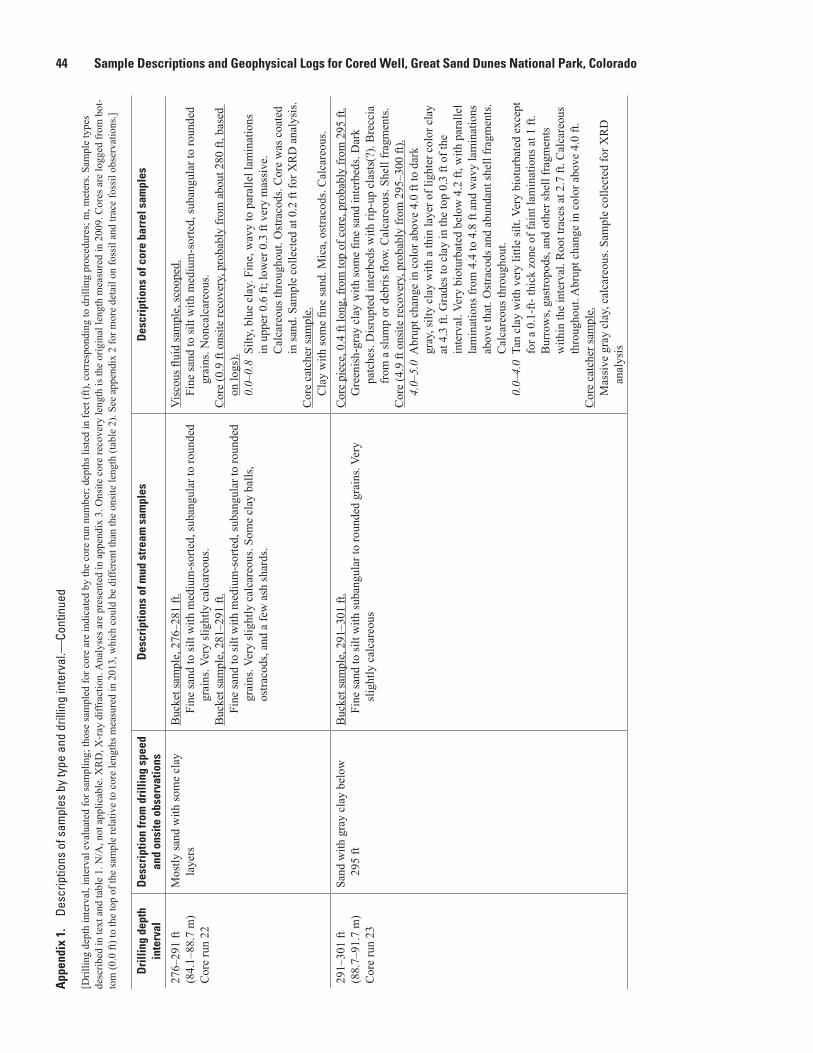
44 Sample Descriptions and Geophysical Logs for Cored Well, Great Sand Dunes National Park, Colorado
Dri
lling
dep
th
inte
rval
Des
crip
tion
from
dri
lling
spe
ed
and
onsi
te o
bser
vatio
nsD
escr
iptio
ns o
f mud
str
eam
sam
ples
Des
crip
tions
of c
ore
barr
el s
ampl
es
276–
291
ft(8
4.1–
88.7
m)
Cor
e ru
n 22
Mos
tly sa
nd w
ith so
me
clay
la
yers
Buc
ket s
ampl
e, 2
76–2
81 ft
. Fi
ne sa
nd to
silt
with
med
ium
-sor
ted,
suba
ngul
ar to
roun
ded
grai
ns. V
ery
slig
htly
cal
care
ous.
Buc
ket s
ampl
e, 2
81–2
91 ft
. Fi
ne sa
nd to
silt
with
med
ium
-sor
ted,
suba
ngul
ar to
roun
ded
grai
ns. V
ery
slig
htly
cal
care
ous.
Som
e cl
ay b
alls
,
ostra
cods
, and
a fe
w a
sh sh
ards
.
Vis
cous
flui
d sa
mpl
e, sc
oope
d.
Fine
sand
to si
lt w
ith m
ediu
m-s
orte
d, su
bang
ular
to ro
unde
d
gr
ains
. Non
calc
areo
us.
Cor
e (0
.9 ft
ons
ite re
cove
ry, p
roba
bly
from
abo
ut 2
80 ft
, bas
ed
on lo
gs).
0.
0–0.
8 Si
lty, b
lue
clay
. Fin
e, w
avy
to p
aral
lel l
amin
atio
ns
i
n up
per 0
.6 ft
; low
er 0
.3 ft
ver
y m
assi
ve.
C
alca
reou
s thr
ough
out.
Ost
raco
ds. C
ore
was
coa
ted
in
sand
. Sam
ple
colle
cted
at 0
.2 ft
for X
RD
ana
lysi
s. C
ore
catc
her s
ampl
e.
Cla
y w
ith so
me
fine
sand
. Mic
a, o
stra
cods
. Cal
care
ous.
291–
301
ft(8
8.7–
91.7
m)
Cor
e ru
n 23
Sand
with
gra
y cl
ay b
elow
29
5 ft
Buc
ket s
ampl
e, 2
91–3
01 ft
. Fi
ne sa
nd to
silt
with
suba
ngul
ar to
roun
ded
grai
ns. V
ery
slig
htly
cal
care
ous
Cor
e pi
ece,
0.4
ft lo
ng, f
rom
top
of c
ore,
pro
babl
y fr
om 2
95 ft
. G
reen
ish-
gray
cla
y w
ith so
me
fine
sand
inte
rbed
s. D
ark
patc
hes.
Dis
rupt
ed in
terb
eds w
ith ri
p-up
cla
sts(
?). B
recc
ia
fr
om a
slum
p or
deb
ris fl
ow. C
alca
reou
s. Sh
ell f
ragm
ents
.C
ore
(4.9
ft o
nsite
reco
very
, pro
babl
y fr
om 2
95–3
00 ft
).
4.0–
5.0
Abr
upt c
hang
e in
col
or a
bove
4.0
ft to
dar
k
g
ray,
silty
cla
y w
ith a
thin
laye
r of l
ight
er c
olor
cla
y
a
t 4.3
ft. G
rade
s to
clay
in th
e to
p 0.
3 ft
of th
e
i
nter
val.
Very
bio
turb
ated
bel
ow 4
.2 ft
, with
par
alle
l
lam
inat
ions
from
4.4
to 4
.8 ft
and
wav
y la
min
atio
ns
a
bove
that
. Ost
raco
ds a
nd a
bund
ant s
hell
frag
men
ts.
C
alca
reou
s thr
ough
out.
0.
0–4.
0 Ta
n cl
ay w
ith v
ery
little
silt.
Ver
y bi
otur
bate
d ex
cept
for
a 0
.1-f
t- th
ick
zone
of f
aint
lam
inat
ions
at 1
ft.
B
urro
ws,
gast
ropo
ds, a
nd o
ther
shel
l fra
gmen
ts
w
ithin
the
inte
rval
. Roo
t tra
ces a
t 2.7
ft. C
alca
reou
s
thr
ough
out.
Abr
upt c
hang
e in
col
or a
bove
4.0
ft.
Cor
e ca
tche
r sam
ple.
M
assi
ve g
ray
clay
, cal
care
ous.
Sam
ple
colle
cted
for X
RD
anal
ysis
App
endi
x 1.
De
scrip
tions
of s
ampl
es b
y ty
pe a
nd d
rillin
g in
terv
al.—
Cont
inue
d
[Dril
ling
dept
h in
terv
al, i
nter
val e
valu
ated
for s
ampl
ing;
thos
e sa
mpl
ed fo
r cor
e ar
e in
dica
ted
by th
e co
re ru
n nu
mbe
r; de
pths
list
ed in
feet
(ft),
cor
resp
ondi
ng to
dril
ling
proc
edur
es; m
, met
ers.
Sam
ple
type
s de
scrib
ed in
text
and
tabl
e 1.
N/A
, not
app
licab
le. X
RD
, X-r
ay d
iffra
ctio
n. A
naly
ses a
re p
rese
nted
in a
ppen
dix
3. O
nsite
cor
e re
cove
ry le
ngth
is th
e or
igin
al le
ngth
mea
sure
d in
200
9. C
ores
are
logg
ed fr
om b
ot-
tom
(0.0
ft) t
o th
e to
p of
the
sam
ple
rela
tive
to c
ore
leng
ths m
easu
red
in 2
013,
whi
ch c
ould
be
diffe
rent
than
the
onsi
te le
ngth
(tab
le 2
). Se
e ap
pend
ix 2
for m
ore
deta
il on
foss
il an
d tra
ce fo
ssil
obse
rvat
ions
.]
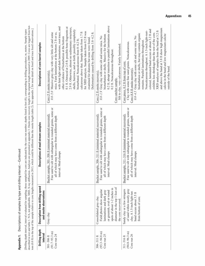
Appendixes 45
Dri
lling
dep
th
inte
rval
Des
crip
tion
from
dri
lling
spe
ed
and
onsi
te o
bser
vatio
nsD
escr
iptio
ns o
f mud
str
eam
sam
ples
Des
crip
tions
of c
ore
barr
el s
ampl
es
301–
306
ft(9
1.7–
93.3
m)
Cor
e ru
n 24
Gra
y cl
ayB
ucke
t sam
ple,
301
–306
ft (m
inim
al m
ater
ial r
ecov
ered
).
Fine
sand
to si
lt w
ith su
bang
ular
to ro
unde
d gr
ains
, som
e or
all o
f whi
ch m
ay h
ave
com
e fr
om a
diff
eren
t dep
th
in
terv
al. M
ud c
lum
ps
Cor
e (5
ft o
nsite
reco
very
).
0.0–
5.0
Mas
sive
gra
y cl
ay w
ith v
ery
little
silt
and
som
e
m
ica.
Fai
nt la
min
atio
ns a
t the
bot
tom
2 ft
or s
o,
w
ith fa
int l
ight
and
dar
k la
min
atio
ns, r
oot t
race
, and
oth
er e
vide
nce
of b
iotu
rbat
ion
at th
e bo
ttom
0.1
ft. O
stra
cod
at 2
.4 ft
; pos
sibl
e bo
ne fr
agm
ents
at
2
.9 ft
. Oth
erw
ise,
alm
ost n
o se
dim
enta
ry st
ruct
ures
,
she
lls, b
urro
ws,
and
so fo
rth; p
ossi
bly
com
plet
ely
bio
turb
ated
. Non
calc
areo
us fr
om 0
–4.2
ft;
c
alca
reou
s abo
ve th
at. S
ampl
e ta
ken
from
1.7
ft
f
or X
RD
ana
lysi
s. Sa
mpl
e ta
ken
from
0.2
ft w
as
e
xam
ined
for d
iato
ms b
ut n
one
wer
e fo
und.
Def
orm
atio
n ca
used
by
drill
ing
from
3.8
–4.2
ft.
306–
311
ft(9
3.3–
94.8
m)
Cor
e ru
n 25
Con
solid
ated
gra
y cl
ay.
Fiel
d ph
otos
show
ang
ular
la
min
atio
ns a
nd d
ark
gray
or
gre
enis
h, o
val o
r rou
nd
spot
s of a
bout
1-2
inch
es in
di
amet
er in
the
top
1 fo
ot o
f th
e co
re re
cove
red.
Buc
ket s
ampl
e, 3
06–3
11 ft
(min
imal
mat
eria
l rec
over
ed).
Fi
ne sa
nd to
silt
with
suba
ngul
ar to
roun
ded
grai
ns, s
ome
or
al
l of w
hich
may
hav
e co
me
from
a d
iffer
ent d
epth
inte
rval
. Mud
clu
mps
Cor
e (2
ft o
nsite
reco
very
).
0.0–
1.9
Gra
y cl
ay w
ith so
me
silt
and
som
e m
ica.
No
bio
turb
atio
n or
shel
ls. M
assi
ve fo
r the
bot
tom
0.2
ft; a
brup
t tra
nsiti
on to
par
alle
l lam
inat
ions
abo
ve
0
.2 ft
. Non
calc
areo
us th
roug
hout
. C
ore
catc
her s
ampl
e.
Silt
to c
lay,
ver
y ca
lcar
eous
. Fai
ntly
lam
inat
ed.
311–
316
ft(9
4.8–
96.3
m)
Cor
e ru
n 26
Sand
y cl
ay o
r a fe
w st
ringe
rs
of sa
nd w
ithin
mos
tly g
ray
clay
. A 1
.5-in
ch li
ght-t
an
band
occ
urs a
bout
3.5
ft
from
bot
tom
of c
ore.
Buc
ket s
ampl
e, 3
11–3
16 ft
(min
imal
mat
eria
l rec
over
ed).
Fi
ne sa
nd to
silt
with
suba
ngul
ar to
roun
ded
grai
ns, s
ome
or
al
l of w
hich
may
hav
e co
me
from
a d
iffer
ent d
epth
inte
rval
. Mud
clu
mps
Cor
e pi
ece,
0.2
ft fr
om to
p of
cor
e.
Cla
y w
ith so
me
fine
sand
gra
ins.
Non
calc
areo
us.
Cor
e (4
.8 ft
ons
ite re
cove
ry).
0.
0–4.
5 G
ray
clay
with
som
e si
lt an
d so
me
mic
a. N
o
b
iotu
rbat
ion
or sh
ells
, but
may
con
tain
org
anic
rem
ains
. Par
alle
l lam
inat
ions
thro
ugho
ut.
N
onca
lcar
eous
thro
ugho
ut. A
1.5
-inch
ligh
t-rus
t-
col
ored
, lam
inat
ed b
and
occu
rs a
t abo
ut 3
.2 ft
and
exh
ibits
less
shrin
kage
than
the
rest
of t
he c
ore.
XR
D a
naly
ses o
f sam
ples
from
the
band
at 3
.2 ft
and
abo
ve th
e ba
nd a
t 3.8
ft sh
ow h
igh
mag
nesi
um
c
alci
te in
the
band
and
low
mag
nesi
um c
alci
te
o
utsi
de o
f the
ban
d.
App
endi
x 1.
De
scrip
tions
of s
ampl
es b
y ty
pe a
nd d
rillin
g in
terv
al.—
Cont
inue
d
[Dril
ling
dept
h in
terv
al, i
nter
val e
valu
ated
for s
ampl
ing;
thos
e sa
mpl
ed fo
r cor
e ar
e in
dica
ted
by th
e co
re ru
n nu
mbe
r; de
pths
list
ed in
feet
(ft),
cor
resp
ondi
ng to
dril
ling
proc
edur
es; m
, met
ers.
Sam
ple
type
s de
scrib
ed in
text
and
tabl
e 1.
N/A
, not
app
licab
le. X
RD
, X-r
ay d
iffra
ctio
n. A
naly
ses a
re p
rese
nted
in a
ppen
dix
3. O
nsite
cor
e re
cove
ry le
ngth
is th
e or
igin
al le
ngth
mea
sure
d in
200
9. C
ores
are
logg
ed fr
om b
ot-
tom
(0.0
ft) t
o th
e to
p of
the
sam
ple
rela
tive
to c
ore
leng
ths m
easu
red
in 2
013,
whi
ch c
ould
be
diffe
rent
than
the
onsi
te le
ngth
(tab
le 2
). Se
e ap
pend
ix 2
for m
ore
deta
il on
foss
il an
d tra
ce fo
ssil
obse
rvat
ions
.]

46 Sample Descriptions and Geophysical Logs for Cored Well, Great Sand Dunes National Park, ColoradoA
ppen
dix
1.
Desc
riptio
ns o
f sam
ples
by
type
and
dril
ling
inte
rval
.—Co
ntin
ued
[Dril
ling
dept
h in
terv
al, i
nter
val e
valu
ated
for s
ampl
ing;
thos
e sa
mpl
ed fo
r cor
e ar
e in
dica
ted
by th
e co
re ru
n nu
mbe
r; de
pths
list
ed in
feet
(ft),
cor
resp
ondi
ng to
dril
ling
proc
edur
es; m
, met
ers.
Sam
ple
type
s de
scrib
ed in
text
and
tabl
e 1.
N/A
, not
app
licab
le. X
RD
, X-r
ay d
iffra
ctio
n. A
naly
ses a
re p
rese
nted
in a
ppen
dix
3. O
nsite
cor
e re
cove
ry le
ngth
is th
e or
igin
al le
ngth
mea
sure
d in
200
9. C
ores
are
logg
ed fr
om b
ot-
tom
(0.0
ft) t
o th
e to
p of
the
sam
ple
rela
tive
to c
ore
leng
ths m
easu
red
in 2
013,
whi
ch c
ould
be
diffe
rent
than
the
onsi
te le
ngth
(tab
le 2
). Se
e ap
pend
ix 2
for m
ore
deta
il on
foss
il an
d tra
ce fo
ssil
obse
rvat
ions
.]
Dri
lling
dep
th
inte
rval
Des
crip
tion
from
dri
lling
spe
ed
and
onsi
te o
bser
vatio
nsD
escr
iptio
ns o
f mud
str
eam
sam
ples
Des
crip
tions
of c
ore
barr
el s
ampl
es
316–
321
ft(9
6.3–
97.8
m)
Cor
e ru
n 27
Gra
y cl
ay w
ith a
coa
rser
gr
aine
d la
yer a
bout
1.5
ft
from
the
top
of th
e co
re.
Buc
ket s
ampl
e, 3
16–3
21 ft
(min
imal
mat
eria
l rec
over
ed).
Fi
ne sa
nd to
silt
with
suba
ngul
ar to
roun
ded
grai
ns, s
ome
or
al
l of w
hich
may
hav
e co
me
from
a d
iffer
ent d
epth
inte
rval
. Mud
clu
mps
Cor
e (5
ft o
nsite
reco
very
).
0.0–
4.5
Gra
y cl
ay w
ith v
ery
little
silt
and
som
e m
ica.
Non
calc
areo
us th
roug
hout
. Par
alle
l lam
inat
ions
thr
ough
out.
The
botto
m 2
.8 ft
con
sist
s of m
any
lig
ht-c
olor
ed la
min
atio
ns a
bout
2 m
illim
eter
s
thi
ck; n
o pa
ttern
is o
bser
ved.
A fe
w o
stra
cods
and
oth
er sh
ells
obs
erve
d w
ithin
2.5
–4.4
ft. A
thin
bed
of b
ival
ves a
nd p
ossi
ble
gast
ropo
ds a
t 3.1
ft is
sur
roun
ded
by li
ght-r
ust-c
olor
ed se
dim
ent.
Poss
ible
lig
ht-r
ust-c
olor
ed o
val b
urro
w a
t 4.4
ft. S
ampl
e
t
aken
from
0.7
ft w
as e
xam
ined
for d
iato
ms b
ut
n
one
wer
e fo
und.
C
ore
piec
e, 0
.1 ft
from
bot
tom
of c
ore.
C
lay
with
som
e fin
e sa
nd g
rain
s. N
onca
lcar
eous
.32
1–32
6 ft
(97.
8–99
.4 m
)C
ore
run
28
Gra
y cl
ay. T
he to
p 2.
7 ft
of
the
core
was
def
orm
ed fr
om
drill
ing
Buc
ket s
ampl
e, 3
21–3
26 ft
(min
imal
mat
eria
l rec
over
ed).
Fi
ne sa
nd to
silt
with
suba
ngul
ar to
roun
ded
grai
ns, s
ome
or
al
l of w
hich
may
hav
e co
me
from
a d
iffer
ent d
epth
inte
rval
. Ost
raco
ds a
nd g
astro
pod
frag
men
ts
Cor
e (4
.6 ft
ons
ite re
cove
ry).
0.
0–4.
3 G
ray
clay
with
som
e si
lt an
d le
ss m
ica
than
abo
ve.
S
light
ly c
alca
reou
s. N
o sa
nd in
terb
eds.
No
lam
inat
ions
vis
ible
, but
diffi
cult
to te
ll be
caus
e th
e
c
ore
was
def
orm
ed b
y dr
illin
g fr
om 1
.6 to
4.3
ft. A
lig
ht-r
ust-c
olor
ed b
ed a
t 2.5
ft is
ver
y ca
lcar
eous
.
Sam
ple
take
n fo
r XR
D a
naly
sis a
t 2.7
ft.
Cor
e ca
tche
r sam
ple.
Si
lt to
cla
y w
ith li
ght a
nd d
ark
lam
inat
ions
. Non
calc
areo
us.
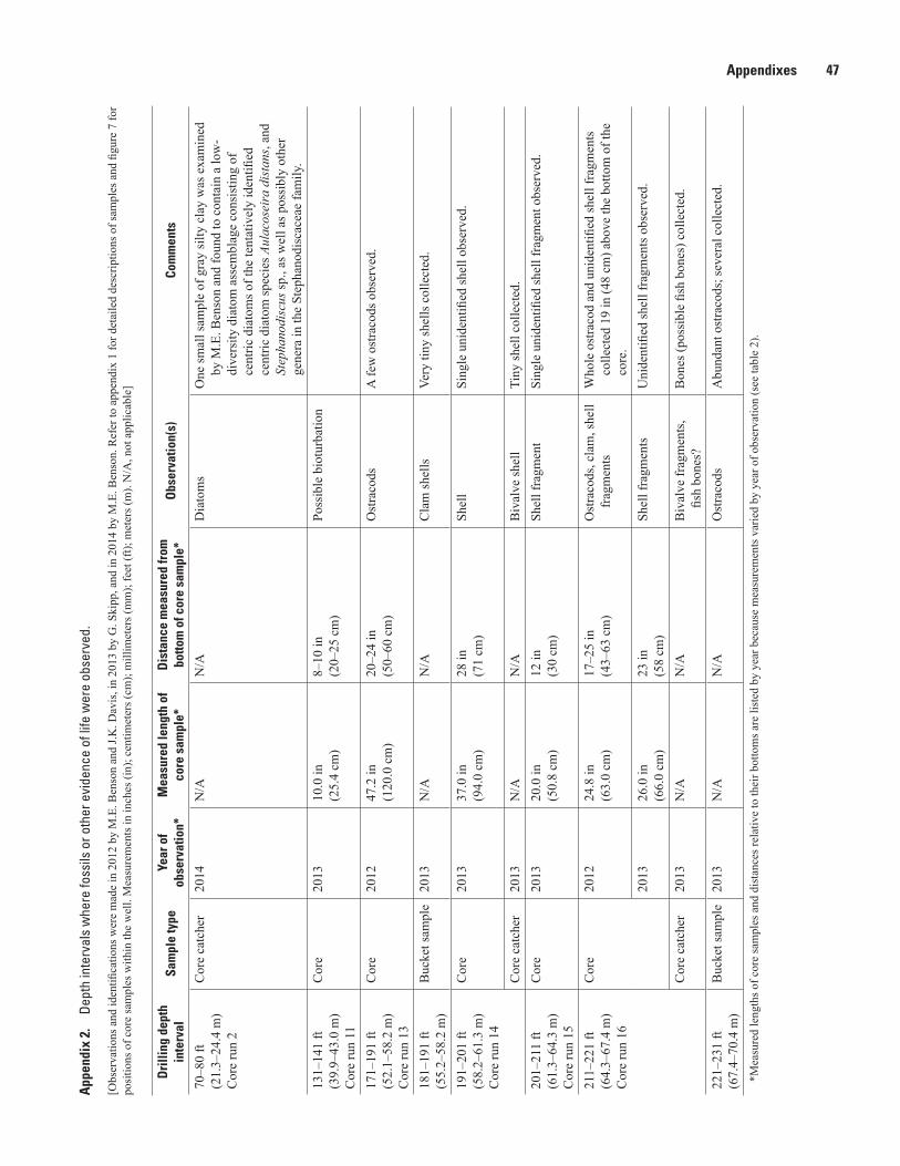
Appendixes 47A
ppen
dix
2.
Dept
h in
terv
als
whe
re fo
ssils
or o
ther
evi
denc
e of
life
wer
e ob
serv
ed.
[Obs
erva
tions
and
iden
tifica
tions
wer
e m
ade
in 2
012
by M
.E. B
enso
n an
d J.K
. Dav
is, i
n 20
13 b
y G
. Ski
pp, a
nd in
201
4 by
M.E
. Ben
son.
Ref
er to
app
endi
x 1
for d
etai
led
desc
riptio
ns o
f sam
ples
and
figu
re 7
for
posi
tions
of c
ore
sam
ples
with
in th
e w
ell.
Mea
sure
men
ts in
inch
es (i
n); c
entim
eter
s (cm
); m
illim
eter
s (m
m);
feet
(ft);
met
ers (
m).
N/A
, not
app
licab
le]
Dri
lling
dep
th
inte
rval
Sam
ple
type
Year
of
obse
rvat
ion*
Mea
sure
d le
ngth
of
core
sam
ple*
Dis
tanc
e m
easu
red
from
bo
ttom
of c
ore
sam
ple*
Obs
erva
tion(
s)Co
mm
ents
70–8
0 ft
(21.
3–24
.4 m
)C
ore
run
2
Cor
e ca
tche
r20
14N
/AN
/AD
iato
ms
One
smal
l sam
ple
of g
ray
silty
cla
y w
as e
xam
ined
by
M.E
. Ben
son
and
foun
d to
con
tain
a lo
w-
dive
rsity
dia
tom
ass
embl
age
cons
istin
g of
ce
ntric
dia
tom
s of t
he te
ntat
ivel
y id
entifi
ed
cent
ric d
iato
m sp
ecie
s Aul
acos
eira
dis
tans
, and
St
epha
nodi
scus
sp.,
as w
ell a
s pos
sibl
y ot
her
gene
ra in
the
Step
hano
disc
acea
e fa
mily
.13
1–14
1 ft
(39.
9–43
.0 m
)C
ore
run
11
Cor
e20
1310
.0 in
(25.
4 cm
)8–
10 in
(20–
25 c
m)
Poss
ible
bio
turb
atio
n
171–
191
ft(5
2.1–
58.2
m)
Cor
e ru
n 13
Cor
e20
1247
.2 in
(120
.0 c
m)
20–2
4 in
(50–
60 c
m)
Ost
raco
ds
A fe
w o
stra
cods
obs
erve
d.
181–
191
ft(5
5.2–
58.2
m)
Buc
ket s
ampl
e20
13N
/AN
/AC
lam
shel
ls
Very
tiny
shel
ls c
olle
cted
.
191–
201
ft(5
8.2–
61.3
m)
Cor
e ru
n 14
Cor
e20
1337
.0 in
(94.
0 cm
)28
in(7
1 cm
)Sh
ell
Sing
le u
nide
ntifi
ed sh
ell o
bser
ved.
Cor
e ca
tche
r20
13N
/AN
/AB
ival
ve sh
ell
Tiny
shel
l col
lect
ed.
201–
211
ft(6
1.3–
64.3
m)
Cor
e ru
n 15
Cor
e 20
1320
.0 in
(50.
8 cm
)12
in(3
0 cm
)Sh
ell f
ragm
ent
Sing
le u
nide
ntifi
ed sh
ell f
ragm
ent o
bser
ved.
211–
221
ft(6
4.3–
67.4
m)
Cor
e ru
n 16
Cor
e20
1224
.8 in
(63.
0 cm
)17
–25
in(4
3–63
cm
)O
stra
cods
, cla
m, s
hell
frag
men
tsW
hole
ost
raco
d an
d un
iden
tified
shel
l fra
gmen
ts
colle
cted
19
in (4
8 cm
) abo
ve th
e bo
ttom
of t
he
core
.20
1326
.0 in
(66.
0 cm
)23
in(5
8 cm
)Sh
ell f
ragm
ents
Uni
dent
ified
shel
l fra
gmen
ts o
bser
ved.
Cor
e ca
tche
r20
13N
/AN
/AB
ival
ve fr
agm
ents
, fis
h bo
nes?
Bon
es (p
ossi
ble
fish
bone
s) c
olle
cted
.
221–
231
ft(6
7.4–
70.4
m)
Buc
ket s
ampl
e20
13N
/AN
/AO
stra
cods
Abu
ndan
t ost
raco
ds; s
ever
al c
olle
cted
.
*Mea
sure
d le
ngth
s of c
ore
sam
ples
and
dis
tanc
es re
lativ
e to
thei
r bot
tom
s are
list
ed b
y ye
ar b
ecau
se m
easu
rem
ents
var
ied
by y
ear o
f obs
erva
tion
(see
tabl
e 2)
.

48 Sample Descriptions and Geophysical Logs for Cored Well, Great Sand Dunes National Park, Colorado
Dri
lling
dep
th
inte
rval
Sam
ple
type
Year
of
obse
rvat
ion*
Mea
sure
d le
ngth
of
core
sam
ple*
Dis
tanc
e m
easu
red
from
bo
ttom
of c
ore
sam
ple*
Obs
erva
tion(
s)Co
mm
ents
231–
241
ft(7
0.4–
73.5
m)
Cor
e ru
n 17
Cor
e (to
p pi
ece)
2012
55.9
in(1
42.0
cm
)52
in(1
32 c
m)
Ost
raco
ds
46 in
(118
cm
)Fo
ssil
Uni
dent
ified
foss
il co
llect
ed.
36–5
6 in
(92–
142
cm)
Ost
raco
d, u
nkno
wn
whi
te c
ircul
ar
grai
ns
Unk
now
n fin
e w
hite
circ
ular
gra
ins m
ay o
r may
not
be
foss
ils.
34 in
(86
cm)
Poss
ible
gas
tropo
dPo
ssib
le g
astro
pod
colle
cted
.
33–3
5 in
(84–
89 c
m)
Shel
l fra
gmen
tsU
nide
ntifi
ed sh
ell f
ragm
ents
col
lect
ed.
32–3
6 in
(82–
92 c
m)
Gas
tropo
dsA
few
gas
tropo
ds w
ere
obse
rved
.
13 in
(32
cm)
Gas
tropo
ds,
biot
urba
tion
9 in
(24
cm)
Bur
row
Bur
row
sam
pled
.
5 in
(12
cm)
Poss
ible
bla
ck sh
ells
Bla
ck-c
olor
ed sp
ecim
ens t
hat m
ay b
e sh
ells
wer
e co
llect
ed.
4–13
in
(9–3
2 cm
)G
astro
pod,
unk
now
n w
hite
circ
ular
gr
ains
Unk
now
n fin
e w
hite
circ
ular
gra
ins m
ay o
r may
not
be
foss
ils.
2 in
(4 c
m)
Car
bon
resi
due,
w
oody
pla
nt
frag
men
ts, t
ooth
or
bone
frag
men
ts20
1357
.5 in
(146
.1 c
m)
10 in
(25
cm)
Poss
ible
bio
turb
atio
nPo
ssib
le b
iotu
rbat
ion
indi
cate
d by
1-c
m-s
ize
oval
s w
ith ru
st-c
olor
ed h
aloe
s.
App
endi
x 2.
De
pth
inte
rval
s w
here
foss
ils o
r oth
er e
vide
nce
of li
fe w
ere
obse
rved
.—Co
ntin
ued
[Obs
erva
tions
and
iden
tifica
tions
wer
e m
ade
in 2
012
by M
.E. B
enso
n an
d J.K
. Dav
is, i
n 20
13 b
y G
. Ski
pp, a
nd in
201
4 by
M.E
. Ben
son.
Ref
er to
app
endi
x 1
for d
etai
led
desc
riptio
ns o
f sam
ples
and
figu
re 7
for
posi
tions
of c
ore
sam
ples
with
in th
e w
ell.
Mea
sure
men
ts in
inch
es (i
n); c
entim
eter
s (cm
); m
illim
eter
s (m
m);
feet
(ft);
met
ers (
m).
N/A
, not
app
licab
le]
*Mea
sure
d le
ngth
s of c
ore
sam
ples
and
dis
tanc
es re
lativ
e to
thei
r bot
tom
s are
list
ed b
y ye
ar b
ecau
se m
easu
rem
ents
var
ied
by y
ear o
f obs
erva
tion
(see
tabl
e 2)
.
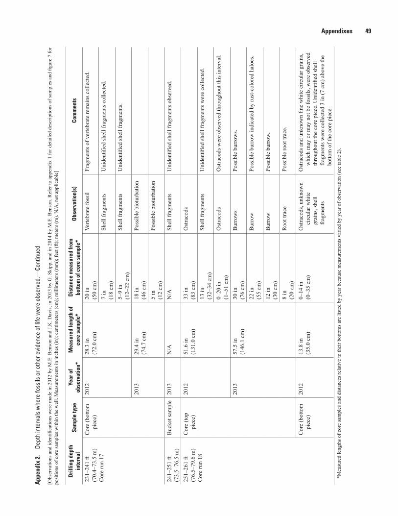
Appendixes 49
Dri
lling
dep
th
inte
rval
Sam
ple
type
Year
of
obse
rvat
ion*
Mea
sure
d le
ngth
of
core
sam
ple*
Dis
tanc
e m
easu
red
from
bo
ttom
of c
ore
sam
ple*
Obs
erva
tion(
s)Co
mm
ents
231–
241
ft(7
0.4–
73.5
m)
Cor
e ru
n 17
Cor
e (b
otto
m
piec
e)20
1228
.3 in
(72.
0 cm
)20
in(5
0 cm
)Ve
rtebr
ate
foss
ilFr
agm
ents
of v
erte
brat
e re
mai
ns c
olle
cted
.
7 in
(18
cm)
Shel
l fra
gmen
tsU
nide
ntifi
ed sh
ell f
ragm
ents
col
lect
ed.
5–9
in(1
2–22
cm
)Sh
ell f
ragm
ents
Uni
dent
ified
shel
l fra
gmen
ts.
2013
29.4
in(7
4.7
cm)
18 in
(46
cm)
Poss
ible
bio
turb
atio
n
5 in
(12
cm)
Poss
ible
bio
turb
atio
n
241–
251
ft(7
3.5–
76.5
m)
Buc
ket s
ampl
e20
13N
/AN
/ASh
ell f
ragm
ents
Uni
dent
ified
shel
l fra
gmen
ts o
bser
ved.
251–
261
ft(7
6.5–
79.6
m)
Cor
e ru
n 18
Cor
e (to
p pi
ece)
2012
51.6
in(1
31.0
cm
)33
in(8
3 cm
)O
stra
cods
13 in
(32–
34 c
m)
Shel
l fra
gmen
tsU
nide
ntifi
ed sh
ell f
ragm
ents
wer
e co
llect
ed.
0–20
in(1
–51
cm)
Ost
raco
dsO
stra
cods
wer
e ob
serv
ed th
roug
hout
this
inte
rval
.
2013
57.5
in(1
46.1
cm
)30
in(7
6 cm
)B
urro
ws
Poss
ible
bur
row
s.
22 in
(55
cm)
Bur
row
Poss
ible
bur
row
indi
cate
d by
rust
-col
ored
hal
oes.
12 in
(30
cm)
Bur
row
Poss
ible
bur
row
.
8 in
(20
cm)
Roo
t tra
cePo
ssib
le ro
ot tr
ace.
Cor
e (b
otto
m
piec
e)20
1213
.8 in
(35.
0 cm
)0–
14 in
(0–3
5 cm
)O
stra
cods
, unk
now
n ci
rcul
ar w
hite
gr
ains
, she
ll fr
agm
ents
Ost
raco
ds a
nd u
nkno
wn
fine
whi
te c
ircul
ar g
rain
s, w
hich
may
or m
ay n
ot b
e fo
ssils
, wer
e ob
serv
ed
thro
ugho
ut th
e co
re p
iece
. Uni
dent
ified
shel
l fr
agm
ents
wer
e co
llect
ed 3
in (7
cm
) abo
ve th
e bo
ttom
of t
he c
ore
piec
e.
App
endi
x 2.
De
pth
inte
rval
s w
here
foss
ils o
r oth
er e
vide
nce
of li
fe w
ere
obse
rved
.—Co
ntin
ued
[Obs
erva
tions
and
iden
tifica
tions
wer
e m
ade
in 2
012
by M
.E. B
enso
n an
d J.K
. Dav
is, i
n 20
13 b
y G
. Ski
pp, a
nd in
201
4 by
M.E
. Ben
son.
Ref
er to
app
endi
x 1
for d
etai
led
desc
riptio
ns o
f sam
ples
and
figu
re 7
for
posi
tions
of c
ore
sam
ples
with
in th
e w
ell.
Mea
sure
men
ts in
inch
es (i
n); c
entim
eter
s (cm
); m
illim
eter
s (m
m);
feet
(ft);
met
ers (
m).
N/A
, not
app
licab
le]
*Mea
sure
d le
ngth
s of c
ore
sam
ples
and
dis
tanc
es re
lativ
e to
thei
r bot
tom
s are
list
ed b
y ye
ar b
ecau
se m
easu
rem
ents
var
ied
by y
ear o
f obs
erva
tion
(see
tabl
e 2)
.

50 Sample Descriptions and Geophysical Logs for Cored Well, Great Sand Dunes National Park, Colorado
Dri
lling
dep
th
inte
rval
Sam
ple
type
Year
of
obse
rvat
ion*
Mea
sure
d le
ngth
of
core
sam
ple*
Dis
tanc
e m
easu
red
from
bo
ttom
of c
ore
sam
ple*
Obs
erva
tion(
s)Co
mm
ents
261–
266
ft(7
9.6–
81.1
m)
Cor
e ru
n 19
Cor
e20
1245
.7 in
(116
.0 c
m)
0–46
in(0
–116
cm
)O
stra
cods
Ost
raco
ds a
bund
ant t
hrou
ghou
t thi
s cor
e sa
mpl
e,
espe
cial
ly a
t 4 in
(10
cm) a
bove
the
botto
m
of th
e sa
mpl
e. S
ampl
es c
olle
cted
at 1
7 in
(43
cm) a
nd 3
6 in
(91
cm) a
bove
the
botto
m o
f the
sa
mpl
e.
34 in
(86
cm)
Dia
tom
s, os
traco
dsA
few
dia
tom
s wer
e pr
esen
t in
a sa
mpl
e co
ntai
ning
os
traco
ds.
M.E
. Ben
son
obse
rved
a lo
w-
dive
rsity
dia
tom
ass
embl
age
dom
inat
ed b
y th
e te
ntat
ivel
y id
entifi
ed sm
all c
entri
c sp
ecie
s Au
laco
seir
a di
stan
s and
the
larg
e pe
nnat
e sp
ecie
s Ano
moe
onei
s sph
aero
phor
a f.
cost
ata.
A
dditi
onal
pen
nate
gen
era,
pos
sibl
y of
the
Ach
nant
hidi
acea
e an
d Fr
agila
riace
ae fa
mili
es,
as w
ell a
s one
spec
imen
rese
mbl
ing
the
genu
s Su
rire
lla, w
ere
also
obs
erve
d.22
–30
in(5
6–76
cm
)Sh
ell f
ragm
ents
Unk
now
n sh
ell f
ragm
ents
.
2013
48.0
in(1
21.9
cm
)44
–46
in(1
12–1
16 c
m)
Ost
raco
dsA
bund
ant o
stra
cods
obs
erve
d w
ithin
a si
lty
inte
rval
.C
ore
catc
her
2013
N/A
N/A
Ost
raco
dsA
bund
ant o
stra
cods
thro
ugho
ut th
e sa
mpl
e.26
6–27
1 ft
(81.
1–82
.6 m
)C
ore
run
20
Cor
e20
1239
.4 in
(100
.0 c
m)
0–39
in(0
–100
cm
)O
stra
cods
Ost
raco
ds a
bund
ant t
hrou
ghou
t the
sam
ple,
with
os
traco
d co
quin
as a
t 10–
11 in
(25–
28 c
m),
25–2
6 in
(64–
65 c
m),
and
30 in
(75
cm) a
bove
th
e bo
ttom
. She
ll fr
agm
ents
and
ost
raco
ds
colle
cted
from
the
low
er tw
o co
quin
as.
35 in
(90
cm)
Unk
now
n sp
ecim
enA
n un
iden
tified
spec
imen
of b
row
n co
lor w
as
colle
cted
.20
1342
.0 in
(106
.7 c
m)
30 in
(76
cm)
Ost
raco
dsO
stra
cod
coqu
ina
abou
t 1 in
(3 c
m) t
hick
.
12 in
(30
cm)
Ost
raco
ds
2 in
(6 c
m)
Ost
raco
ds
Cor
e ca
tche
r20
13N
/AN
/AO
stra
cods
Buc
ket s
ampl
e20
13N
/AN
/AO
stra
cods
App
endi
x 2.
De
pth
inte
rval
s w
here
foss
ils o
r oth
er e
vide
nce
of li
fe w
ere
obse
rved
.—Co
ntin
ued
[Obs
erva
tions
and
iden
tifica
tions
wer
e m
ade
in 2
012
by M
.E. B
enso
n an
d J.K
. Dav
is, i
n 20
13 b
y G
. Ski
pp, a
nd in
201
4 by
M.E
. Ben
son.
Ref
er to
app
endi
x 1
for d
etai
led
desc
riptio
ns o
f sam
ples
and
figu
re 7
for
posi
tions
of c
ore
sam
ples
with
in th
e w
ell.
Mea
sure
men
ts in
inch
es (i
n); c
entim
eter
s (cm
); m
illim
eter
s (m
m);
feet
(ft);
met
ers (
m).
N/A
, not
app
licab
le]
*Mea
sure
d le
ngth
s of c
ore
sam
ples
and
dis
tanc
es re
lativ
e to
thei
r bot
tom
s are
list
ed b
y ye
ar b
ecau
se m
easu
rem
ents
var
ied
by y
ear o
f obs
erva
tion
(see
tabl
e 2)
.

Appendixes 51
Dri
lling
dep
th
inte
rval
Sam
ple
type
Year
of
obse
rvat
ion*
Mea
sure
d le
ngth
of
core
sam
ple*
Dis
tanc
e m
easu
red
from
bo
ttom
of c
ore
sam
ple*
Obs
erva
tion(
s)Co
mm
ents
271–
276
ft(8
2.6–
84.1
m)
Cor
e ru
n 21
Cor
e20
1235
.4 in
(90.
0 cm
)0–
35 in
(0–9
0 cm
)O
stra
cods
Ost
raco
ds o
bser
ved
thro
ugho
ut th
e co
re sa
mpl
e.
They
are
abu
ndan
t 16–
17 in
(41–
42 c
m) a
bove
th
e ba
se o
f the
sam
ple.
Spe
cim
ens c
olle
cted
fr
om 1
7 in
(42
cm) a
nd 1
in (3
cm
) abo
ve th
e bo
ttom
of t
he c
ore
sam
ple.
C
ore
catc
her
2013
N/A
N/A
Ost
raco
ds27
6–29
1 ft
(84.
1–88
.7 m
)C
ore
run
22
Cor
e20
129.
1 in
(23.
0 cm
)0–
9 in
(0–2
3 cm
) O
stra
cods
Ost
raco
ds o
bser
ved
thro
ugho
ut th
e w
hole
sam
ple.
Sp
ecim
ens c
olle
cted
7 in
(17
cm) a
bove
the
botto
m o
f the
cor
e sa
mpl
e.
Cor
e ca
tche
r20
13N
/AN
/AO
stra
cods
291–
301
ft(8
8.7–
91.7
m)
Cor
e ru
n 23
Cor
e pi
ece
at
top
2013
N/A
N/A
Shel
l fra
gmen
tsU
nide
ntifi
ed sh
ell f
ragm
ents
obs
erve
d.
Cor
e20
1257
.9 in
(147
.0 c
m)
50–5
8 in
(127
–147
cm
)O
stra
cods
, she
ll fr
agm
ents
Ost
raco
ds a
nd u
nkno
wn
5-m
m-s
ize
shel
l fra
gmen
ts
obse
rved
. J.K
. Dav
is c
olle
cted
sam
ples
of
ostra
cods
and
oth
er fo
ssils
from
53
in (1
35 c
m)
and
54–5
5 in
(137
–140
cm
). 42
–46
in(1
07–1
17 c
m)
Gas
tropo
ds, s
hell
frag
men
tsG
astro
pods
and
unk
now
n 5-
mm
-siz
e sh
ell
frag
men
ts o
bser
ved.
30–4
2 in
(77–
107
cm)
Shel
l fra
gmen
tsA
few
unk
now
n, 2
-mm
-siz
e sh
ell f
ragm
ents
ob
serv
ed.
32 in
(81
cm)
Bio
turb
atio
n, ro
ot
trace
s, ga
stro
pods
Bio
turb
atio
n, p
ossi
ble
root
trac
es, a
nd fr
agm
ents
of
gast
ropo
ds o
bser
ved.
19
–26
in(4
7–67
cm
)Sh
ell f
ragm
ents
Unk
now
n 1-
mm
-siz
e sh
ell f
ragm
ents
obs
erve
d.
2013
60.0
in(1
52.4
cm
)0–
50 in
(0–1
28 c
m)
Bio
turb
atio
n, b
urro
ws,
shel
l fra
gmen
tsSa
mpl
e sh
ows i
nten
se b
iotu
rbat
ion,
with
bur
row
s at
18
in (4
6 cm
), 19
in (4
9 cm
), 24
in (6
1 cm
), 30
in (7
6 cm
), an
d po
ssib
ly a
t 2 in
(6 c
m) a
bove
bo
ttom
of t
he c
ore,
resp
ectiv
ely.
She
ll fr
agm
ents
w
ere
also
obs
erve
d at
24
in (6
1 cm
). 48
–58
in(1
22–1
47 c
m)
Shel
l fra
gmen
tsA
bund
ant s
hell
frag
men
ts.
17 in
(43
cm)
Gas
tropo
dA
smal
l gas
tropo
d ob
serv
ed.
App
endi
x 2.
De
pth
inte
rval
s w
here
foss
ils o
r oth
er e
vide
nce
of li
fe w
ere
obse
rved
.—Co
ntin
ued
[Obs
erva
tions
and
iden
tifica
tions
wer
e m
ade
in 2
012
by M
.E. B
enso
n an
d J.K
. Dav
is, i
n 20
13 b
y G
. Ski
pp, a
nd in
201
4 by
M.E
. Ben
son.
Ref
er to
app
endi
x 1
for d
etai
led
desc
riptio
ns o
f sam
ples
and
figu
re 7
for
posi
tions
of c
ore
sam
ples
with
in th
e w
ell.
Mea
sure
men
ts in
inch
es (i
n); c
entim
eter
s (cm
); m
illim
eter
s (m
m);
feet
(ft);
met
ers (
m).
N/A
, not
app
licab
le]
*Mea
sure
d le
ngth
s of c
ore
sam
ples
and
dis
tanc
es re
lativ
e to
thei
r bot
tom
s are
list
ed b
y ye
ar b
ecau
se m
easu
rem
ents
var
ied
by y
ear o
f obs
erva
tion
(see
tabl
e 2)
.
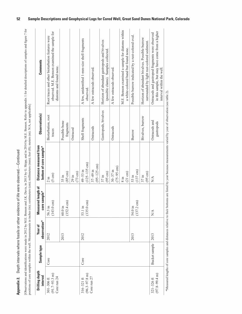
52 Sample Descriptions and Geophysical Logs for Cored Well, Great Sand Dunes National Park, Colorado
Dri
lling
dep
th
inte
rval
Sam
ple
type
Year
of
obse
rvat
ion*
Mea
sure
d le
ngth
of
core
sam
ple*
Dis
tanc
e m
easu
red
from
bo
ttom
of c
ore
sam
ple*
Obs
erva
tion(
s)Co
mm
ents
301–
306
ft(9
1.7–
93.3
m)
Cor
e ru
n 24
Cor
e20
1256
.3 in
(143
.0 c
m)
2 in
(5 c
m)
Bio
turb
atio
n, ro
ot
trace
sR
oot t
race
s and
oth
er b
iotu
rbat
ion
feat
ures
wer
e ob
serv
ed. M
.E. B
enso
n ex
amin
ed th
e sa
mpl
e fo
r di
atom
s and
foun
d no
ne.
2013
60.0
in(1
52.4
cm
)35
in(8
5 cm
)Po
ssib
le b
one
frag
men
ts29
in(7
3 cm
)O
stra
cod
316–
321
ft(9
6.3–
97.8
m)
Cor
e ru
n 27
Cor
e20
1253
.1 in
(135
.0 c
m)
49–5
3 in
(125
–135
cm
)Sh
ell f
ragm
ents
A fe
w, u
nide
ntifi
ed 1
-mm
-siz
e sh
ell f
ragm
ents
ob
serv
ed.
37–4
9 in
(95–
125
cm)
Ost
raco
dsA
few
ost
raco
ds o
bser
ved.
37 in
(95
cm)
Gas
tropo
ds, b
ival
ves
Hor
izon
of a
bund
ant g
astro
pods
and
biv
alve
s (p
ossi
ble
clam
s).
Sam
ples
col
lect
ed.
30–3
7 in
(75–
95 c
m)
Ost
raco
dsA
few
ost
raco
ds o
bser
ved.
8 in
(21
cm)
M.E
. Ben
son
exam
ined
a sa
mpl
e fo
r dia
tom
s with
in
a w
hite
-col
ored
ban
d bu
t fou
nd n
one.
2013
54.0
in(1
37.2
cm
)53
in(1
37 c
m)
Bur
row
Poss
ible
bur
row
indi
cate
d by
a ru
st-c
olor
ed o
val.
37 in
(95
cm)
Biv
alve
s, bu
rrow
Hor
izon
of a
bund
ant b
ival
ves.
Poss
ible
bur
row
su
rrou
nded
by
light
rust
-col
ored
sedi
men
t.32
1–32
6 ft
(97.
8–99
.4 m
)B
ucke
t sam
ple
2013
N/A
N/A
Ost
raco
ds a
nd
gast
ropo
dsO
stra
cods
and
gas
tropo
d fr
agm
ents
wer
e ob
serv
ed
in th
is sa
mpl
e, b
ut m
ay h
ave
com
e fr
om a
hig
her
inte
rval
with
in th
e w
ell.
*Mea
sure
d le
ngth
s of c
ore
sam
ples
and
dis
tanc
es re
lativ
e to
thei
r bot
tom
s are
list
ed b
y ye
ar b
ecau
se m
easu
rem
ents
var
ied
by y
ear o
f obs
erva
tion
(see
tabl
e 2)
.
App
endi
x 2.
De
pth
inte
rval
s w
here
foss
ils o
r oth
er e
vide
nce
of li
fe w
ere
obse
rved
.—Co
ntin
ued
[Obs
erva
tions
and
iden
tifica
tions
wer
e m
ade
in 2
012
by M
.E. B
enso
n an
d J.K
. Dav
is, i
n 20
13 b
y G
. Ski
pp, a
nd in
201
4 by
M.E
. Ben
son.
Ref
er to
app
endi
x 1
for d
etai
led
desc
riptio
ns o
f sam
ples
and
figu
re 7
for
posi
tions
of c
ore
sam
ples
with
in th
e w
ell.
Mea
sure
men
ts in
inch
es (i
n); c
entim
eter
s (cm
); m
illim
eter
s (m
m);
feet
(ft);
met
ers (
m).
N/A
, not
app
licab
le]

Appendixes 53
Appendix 3. Results of analysis by X-ray powder diffraction
[Depth in feet (ft); meters (m); in., inch. Refer to appendix 1 for detailed descriptions of samples. Minerals are listed in order of peak X-ray intensity]
Drilling interval Sample type Description of specimen collected Bulk X-ray minerology
30–40 ft(9.1–12.2 m)
Hopper, fine fraction Fine sand Quartz, anorthite, albite, cristobalite, potassium feldspar, amphibole, mica.
70–80 ft(21.3–24.4 m)
Core catcher Clay from about 77 ft depth Quartz, plagioclase feldspar, calcite, cristobalite, clay, mica.
70–80 ft(21.3–24.4 m)
Core catcher Silt from about 77 ft depth Quartz, plagioclase feldspar, cristobalite, calcite, clay, mica.
80–90 ft(24.4–27.4 m)
Core catcher Very fine sand to clay, possibly from about 85 ft depth
Quartz, albite, cristobalite, potassium feldspar, mica, smectite.
119–125 ft(36.3–38.1 m)
Core catcher Fine sand to silt, probably from somewhere between 121 and 125 ft depth
Quartz, plagioclase feldspar, cristobalite, potassium feldspar, clay, pyrite?
191–201 ft(58.2–61.3 m)
Core Silty clay taken from approximately 2 ft above the bottom of the core
Quartz, plagioclase feldspar, cristobalite, potassium feldspar, clay.
191–201 ft(58.2–61.3 m)
Core Very fine sand taken from the lower foot of the core
Cristobalite, quartz, plagioclase feldspar, mica.
231–241 ft(70.4–73.5 m)
Core Clay taken from 14 in. above the bottom of the bottom core piece, probably at about 239–240 ft depth
Quartz, plagioclase feldspar, cristobalite, calcite, clay, mica, kaolinite.
271–276 ft(82.6–84.1 m)
Core Clay taken from 11 in. above the bottom of the core, at about 273 ft depth
Quartz, calcite, plagioclase feldspar, cristobalite, potassium feldspar, clay, mica.
276–291 ft(84.1–88.7 m)
Core Clay taken from 2 in. above the bottom of the core, probably at about 280 ft depth
Quartz, calcite, plagioclase feldspar, cristobalite, clay, potassium feldspar, mica, kaolinite.
291–301 ft(88.7–91.7 m)
Core catcher Clay from about 300 ft depth Quartz, calcite, plagioclase feldspar, cristobalite, clay, potassium feldspar, mica, kaolinite.
301–306 ft(91.7–93.3 m)
Core Clay taken from 20 in. above the bottom of the core, at about 304 ft depth
Plagioclase feldspar, quartz, cristobalite, dolomite, potassium feldspar, clay, mica, kaolinite.
311–316 ft(94.8–96.3 m)
Core Clay taken at 45 in. from the bottom of the core, sampled above a light-rust-colored band at 38 in. Sample probably from a depth of about 312 ft
Cristobalite, plagioclase feldspar, quartz, potassium feldspar, calcite, clay, kaolinite, mica.
311–316 ft(94.8–96.3 m)
Core Sample taken from a light-rust-colored, laminated band 38 in. above the bottom of the core, probably at about 313 ft depth
High-magnesium calcite, plagioclase feldspar, cristobalite, quartz, potassium feldspar, clay, mica.
321–326 ft(97.8–99.4 m)
Core Clay taken from 32 in. above the bottom of the core, at about 322 ft depth
Quartz, plagioclase feldspar, cristobalite, potassium feldspar, clay, calcite, kaolinite, mica.

Publishing support provided by the U.S. Geological Survey Science Publishing Network, Rolla Publishing Service Center and Denver Publishing Service Center
For more information concerning the research in this report, contact the Director, Crustal Geophysics and Geochemistry Science Center U.S. Geological Survey Box 25046, Mail Stop 964 Denver, CO 80225 http://crustal.usgs.gov/


Grauch and others— Sam
ple Descriptions and G
eophysical Logs for Cored Well, G
reat Sand Dunes N
ational Park, Colorado—Data Series 918
ISSN 2327-638X (online)http://dx.doi.org/10.3133/ds918
Related Documents