SALT INTRUSION IN GATUN LAKE A Major Qualifying … Table of Contents Abstract ..... ii

Project JYP-1104

SALT INTRUSION IN GATUN LAKE

A Major Qualifying Project

submitted to the Faculty

of

WORCESTER POLYTECHNIC INSTITUTE

in partial fulfillment of the requirements for the

Degree of Bachelor of Science

By

Assel Akhmetova

Cristina Crespo

Edwin Muñiz

March 11, 2012

Jeanine D. Plummer, Major Advisor

Associate Professor, Civil and Environmental Engineering

1. Gatun Lake

2. Salt Intrusion

3. Panama Canal

ii

Abstract

The expansion of the Panama Canal is adding another lock lane to the canal, allowing

passage of larger ships. Increases in the number of transits and the size of the locks may displace

more salt from the oceans into the freshwater lake, Gatun Lake, which is a drinking water source

for Panama City. This project evaluated future salinity levels in Gatun Lake. Water quality and

hydrometeorological data were input into a predictive hydrodynamic software package to project

salinity levels in the lake after the new lock system is completed. Modeling results showed that

salinity levels are expected to remain in the freshwater range. In the event that the lake becomes

brackish, the team designed a water treatment plant using electrodialysis reversal for salt removal

and UV light disinfection.

iii

Executive Summary

The Panama Canal runs from the Pacific Ocean in the southeast to the Atlantic Ocean in

the northwest over a watershed area containing the freshwater lake, Gatun Lake. The canal

facilitates the transit of 36 ships daily using three sets of locks, which displace large volumes of

water into and out of Gatun Lake. The displacement of water has the potential to cause salt

intrusion into the freshwater Gatun Lake. The ACP is currently expanding the Panama Canal by

constructing a new series of locks, Post-Panamax locks, which will accommodate the transit of

larger ships through the channel. The ACP does not expect that new locks to change the salinity

levels of Gatun Lake (Jongeling, 2008). However, since the lake acts as a fresh drinking water

source for Colon and Panama City, predicting future salinity levels in the lake is important.

The primary goal of this project was to model future salinity levels in Gatun Lake. In

order to meet this goal, three objectives were completed: (1) collection of current water quality

conditions in the lake, (2) modeling of current salinity levels based on historical data and

comparison of those modeled levels to measured values and (3) modeling of future salinity levels

after the expansion project is complete. First, current lake conditions were measured during a

two-day water quality campaign in which water quality was determined at 13 stations within

Gatun Lake. In-situ data in real-time were collected using a SBE 19plus SEACAT Profiler (Sea-

Bird Electronics, Inc., Bellevue, Washington), which measures conductivity, temperature, and

pressure in marine or fresh-water environments at depths of up to 7,000 meters. Then, water

samples at various depths were collected in bottles and transported to the laboratory for

measurement of salinity. Results showed salinity levels were below 0.5 ppt at all stations,

salinity levels tended to increase below an elevation of 5 meters, and of all stations, Buoy D

showed to have the highest salinity levels at the bottom layers of the lake due to its location in

front of the Gatun Locks.

The second objective was to model current salinity levels. Hydrometeorological data,

including air temperature, wind velocity, runoff, precipitation, and evaporation measurements,

were obtained from ACP for the years 2003 – 2005. Saltwater intrusion and dispersion

simulations were run by inputting these data into hydrodynamic software, Delft3D, which

considers the hydrology within natural as well as artificial environments such as the Panama

Canal lock system. In a contract with ACP, Deltares, the developer of the Delft3D software,

created multiple scenarios to analyze the salt intrusion within the particular environment of

iv

Gatun Lake. Year 2011 salinity levels were predicted using the 2003 – 2005 data and the current

shipping schedules (prior to expansion). Results showed that these salinity levels were consistent

with the in-situ salinity measurements gathered during the water quality campaign, verifying that

the software was representative of the real situation.

The third objective was to model future salinity levels considering the large Post-

Panamax locks and increased ship transits. Predictions were made using hydrometeorological

data from 2003 to 2005 and also for data from 2008 to 2009. For all locations in the lake that

were simulated, future salt levels were within the freshwater range (0 ppt – 0.5 ppt). These

results are consistent with ACP expectations that the expanded lock system will not negatively

impact the water quality in Gatun Lake with regard to salinity.

Delft3D modeling results showed that salt levels within Gatun Lake have remained

consistent and are predicted to stay within the freshwater range, with salt levels less than 0.5 ppt.

However, it is still possible that modeling efforts have not fully captured future water quality

scenarios, or that changes in shipping schedules or operation of the locks could result in

increased salt levels in Gatun Lake after the expansion project is completed. Therefore, a

drinking water treatment plant was designed to produce potable water for the city of Colon and

the Panama City metro area considering a brackish water range of 0.5 ppt to 15 ppt conditions in

Gatun Lake. Panamanian law requires some form of flocculation, coagulation, sedimentation, or

filtration in addition to disinfection. The design complies with Panamanian law, and includes

cartridge filters for pretreatment, an electrodialysis reversal (EDR) system for salt removal and

ultraviolet (UV) light for disinfection.

v

Acknowledgements

The group would like to acknowledge Professor Jeanine Plummer and Professor Tahar

El-Korchi, of the Civil and Environmental Engineering Department at Worcester Polytechnic

Institute, for coordinating our project with the Panama Canal Authority as well as their support

as advisers throughout the project. The group would like to thank Daniel Muschett, of the

Panama Canal Authority, for sponsoring our project in Panama. The group would like to thank

Luis Castaneda, Arismediz Montoya, Guadalupe Ortega, and Jorge Villalaz, of the Panama

Canal Authority, for their constant support and guidance throughout our time in Panama.

vi

Table of Contents

Abstract ........................................................................................................................................... ii

Executive Summary ....................................................................................................................... iii

Acknowledgements ......................................................................................................................... v

List of Figures ................................................................................................................................ ix

List of Tables ................................................................................................................................. xi

1.0 Introduction ............................................................................................................................... 1

2.0 Background ............................................................................................................................... 2

2.1 Panama Canal........................................................................................................................ 2

2.1.1 Construction History ...................................................................................................... 3

2.1.2 Canal: 1914 – 2006 ........................................................................................................ 4

2.1.3 Panama Canal Expansion Project .................................................................................. 4

2.1.4 La Autoridad del Canal de Panamá ............................................................................... 7

2.2 Gatun Lake ............................................................................................................................ 7

2.3 Salt Intrusion ......................................................................................................................... 9

2.3.1 Salt Intrusion in Gatun Lake .......................................................................................... 9

2.3.2 Impacts of Salt Intrusion .............................................................................................. 12

3.0 Hydrometeorological and Water Quality Monitoring of Gatun Lake .................................... 13

3.1 Water Quality Measurement Stations ................................................................................. 13

3.2 Hydrometeorological Measurement Stations ...................................................................... 14

4.0 Salt Water Intrusion Modeling Software ................................................................................ 16

4.1 Delft3D-FLOW ................................................................................................................... 16

4.2 Mass Balance ...................................................................................................................... 18

4.3 Modeling Summary ............................................................................................................ 19

5.0 Methodology ........................................................................................................................... 20

5.1 Historical Hydrometeorological Characteristics ................................................................. 20

5.2 Current Salt Intrusion Conditions ....................................................................................... 20

5.3 Salt Intrusion Modeling ...................................................................................................... 21

vii

5.4 Water Quality in Gatun Lake .............................................................................................. 22

6.0 Results and Analysis ............................................................................................................... 25

6.1 Hydrometeorological Parameter Input Data for Software Simulations .............................. 25

6.1.1 Air Temperature ........................................................................................................... 25

6.1.2 Wind ............................................................................................................................. 26

6.1.3 Precipitation ................................................................................................................. 27

6.1.4 Runoff .......................................................................................................................... 28

6.1.5 Evaporation .................................................................................................................. 30

6.2 Water Quality Campaign Results and Simulation Results for Scenario 0 .......................... 31

6.2.1 BuoyD .......................................................................................................................... 33

6.2.2 GE-1 ............................................................................................................................. 34

6.2.3 P-6 ................................................................................................................................ 35

6.3 Salinity Results for Scenario 1 ............................................................................................ 37

6.3.1 Sabanitas ...................................................................................................................... 38

6.3.2 Mt Hope ....................................................................................................................... 40

6.3.3 Escobal ......................................................................................................................... 41

6.3.4 Gamboa ........................................................................................................................ 42

6.3.5 Paraiso .......................................................................................................................... 43

6.3.6 Gatun Lake ................................................................................................................... 44

7.0 Water Treatment Plant ............................................................................................................ 46

7.1 Plant Specifications ............................................................................................................. 46

7.2 Design Alternatives ............................................................................................................. 47

7.2.1 Electrodialysis and Electrodialysis Reversal ............................................................... 48

7.2.2 Reverse Osmosis .......................................................................................................... 51

7.2.3 Membrane Process Selection ....................................................................................... 52

7.3 Disinfection ......................................................................................................................... 53

7.3.1 Chlorine........................................................................................................................ 54

7.3.2 Chlorine Dioxide .......................................................................................................... 55

7.3.3 Ozone ........................................................................................................................... 55

7.3.4 Ultraviolet Disinfection ............................................................................................... 56

7.3.5 Disinfection Process Selection ..................................................................................... 57

viii

7.4 Water Treatment Plant Design ............................................................................................ 57

8.0 Conclusion .............................................................................................................................. 60

9.0 References ............................................................................................................................... 61

ix

List of Figures

Figure 1: Passage of ships through Panama Canal (BBC News, 2006).......................................... 2

Figure 2: Third Set of Locks Project (Panama Canal Authority, 2006a)........................................ 5

Figure 3: Conceptual Isometric View of the New Locks Complex ................................................ 6

(Panama Canal Authority, 2006b) .................................................................................................. 6

Figure 4: Cross-section of Lock Chamber and Walls, Panama Canal (Balu, 2010) ..................... 10

Figure 5: Water Quality Measurement Stations within Water Basin Area (Jongeling, 2008). .... 14

Figure 6: Water Quality Measurement Sites near Pedro Miguel Locks ....................................... 22

Figure 7: Water Quality Measurement Sites near Gatun Dam and Gatun Locks ......................... 23

Figure 8: Air Temperature comparison 2003-2005, 2008-2010 ................................................... 26

Figure 9: Wind velocity comparison 2003-2005, 2008-2010 ....................................................... 27

Figure 10: Precipitation comparison 2003-2005, 2008-2010 ....................................................... 28

Figure 11: Runoff comparison for three principal rivers 2003-2005, 2008-2010 ........................ 29

Figure 12: Evaporation comparison 2003-2005, 2008-2010 ........................................................ 30

Figure 13: Water Quality Measurement Stations near Gatun Dam and Gatun Locks .................. 32

Figure 14: Delft3D Quickplot Salinity Modeling Results at BuoyD for 2003-2005 .................... 33

Figure 15: Salinity Measurements at BuoyD on December 2, 2011 at 11 am.............................. 33

Figure 16: Quickplot Salinity Modeling Results at GE-1 for 2003-2005 ..................................... 34

Figure 17: Salinity Measurements at GE-1 on December 2, 2011 at 12 pm ................................ 35

Figure 18: Quickplot Salinity Modeling Results at P-6 for 2003-2005 ........................................ 36

Figure 19: Salinity Measurements at P-6 on December 2, 2011 at 1 pm ..................................... 36

Figure 20: Freshwater Intake Stations in Gatun Lake .................................................................. 38

Figure 21: Sabanitas Salt Concentration at Depth 1 m above Bottom ......................................... 39

Figure 22: Sabanitas Salt Concentration at Depth 1 m below Surface ......................................... 39

Figure 23: Mt Hope Salt Concentration at Depth 1 m above Bottom .......................................... 40

Figure 24: Mt Hope Salt Concentration at Depth 1 m below Surface .......................................... 40

Figure 25: Escobal Salt Concentration at Depth 1m above Bottom ............................................. 41

Figure 26: Escobal Salt Concentrations at Depth 1m below Surface ........................................... 41

Figure 27: Gamboa Salt Concentration at Depth 1m above Bottom ............................................ 42

Figure 28: Gamboa Salt Concentration at Depth 1m below Surface ............................................ 43

Figure 29: Paraiso Salt Concentration at Depth 1m above Bottom .............................................. 44

x

Figure 30: Paraiso Salt Concentration at Depth 1 m below Surface............................................. 44

Figure 31: Volume-Averaged Salt Concentration in Gatun Lake ................................................ 45

Figure 32: Electrodialysis Process (EET Corporation, 2009) ....................................................... 49

Figure 33: EDR configuration (Trussell Technologies, 2008) ..................................................... 50

Figure 34: Reverse Osmosis Process (E.S.P. Water Products, 2009) ........................................... 51

Figure 35: Water Treatment Plant Flowchart ............................................................................... 59

xi

List of Tables

Table 1: ACP Hydrometeorological Stations ............................................................................... 15

Table 2: Raw Water Quality in Gatun Lake (ACP, 2010) ............................................................ 47

Table 3: Membrane Types ............................................................................................................ 48

Table 4: Comparison of Electrodialysis Reversal and Reverse Osmosis ..................................... 53

Table 5: Characteristics of Disinfectants (adapted from MWH, 2005) ........................................ 54

Table 6: The Main Characteristics of Abrera and Panama City Water Treatment Plants ............ 58

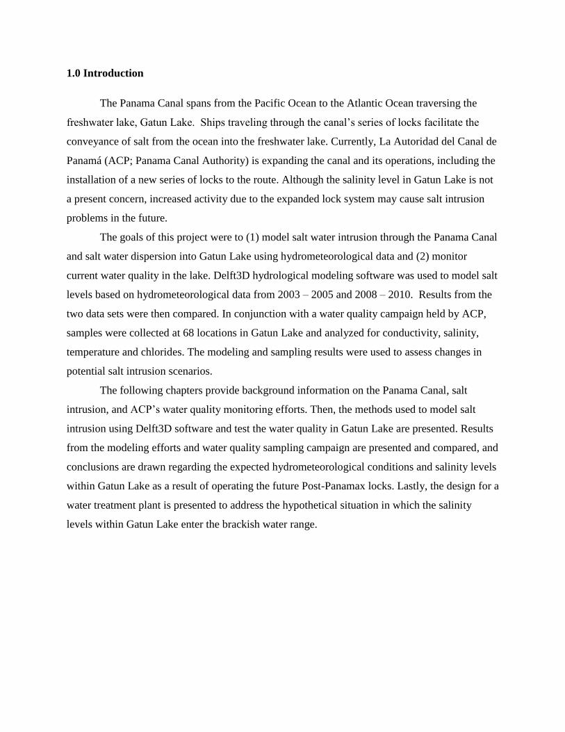
1.0 Introduction

The Panama Canal spans from the Pacific Ocean to the Atlantic Ocean traversing the

freshwater lake, Gatun Lake. Ships traveling through the canal’s series of locks facilitate the

conveyance of salt from the ocean into the freshwater lake. Currently, La Autoridad del Canal de

Panamá (ACP; Panama Canal Authority) is expanding the canal and its operations, including the

installation of a new series of locks to the route. Although the salinity level in Gatun Lake is not

a present concern, increased activity due to the expanded lock system may cause salt intrusion

problems in the future.

The goals of this project were to (1) model salt water intrusion through the Panama Canal

and salt water dispersion into Gatun Lake using hydrometeorological data and (2) monitor

current water quality in the lake. Delft3D hydrological modeling software was used to model salt

levels based on hydrometeorological data from 2003 – 2005 and 2008 – 2010. Results from the

two data sets were then compared. In conjunction with a water quality campaign held by ACP,

samples were collected at 68 locations in Gatun Lake and analyzed for conductivity, salinity,

temperature and chlorides. The modeling and sampling results were used to assess changes in

potential salt intrusion scenarios.

The following chapters provide background information on the Panama Canal, salt

intrusion, and ACP’s water quality monitoring efforts. Then, the methods used to model salt

intrusion using Delft3D software and test the water quality in Gatun Lake are presented. Results

from the modeling efforts and water quality sampling campaign are presented and compared, and

conclusions are drawn regarding the expected hydrometeorological conditions and salinity levels

within Gatun Lake as a result of operating the future Post-Panamax locks. Lastly, the design for a

water treatment plant is presented to address the hypothetical situation in which the salinity

levels within Gatun Lake enter the brackish water range.

2

2.0 Background

A modern engineering marvel, the Panama Canal facilitates global trade and cross-

oceanic travel as it runs southeast to northwest from the Pacific to the Atlantic Ocean (see Figure

1). A freshwater lake, Gatun Lake, comprises the largest part of the naval transit between the two

oceans. Through a series of locks, ships entering via the Pacific Ocean are raised 26 meters

above sea level into Gatun Lake and are then lowered on the northwest end into the Atlantic

Ocean. To meet the ever-growing demands of maritime trade and to accommodate the transit of

larger vessels, the ACP, which maintains sole ownership of the canal, approved the Panama

Canal expansion program in 2006. The expansion will add a third series of locks to the canal.

Since ships travel from the saltwater Pacific and Atlantic Oceans to the freshwater of Gatun

Lake, salt intrusion is a potential concern with the canal expansion.

Figure 1: Passage of ships through Panama Canal (BBC News, 2006)

2.1 Panama Canal

The construction of Panama Canal was an exceptional accomplishment of engineering

that affected the lives of thousands of people. Multiple countries were involved in the planning,

3

design and construction, including Spain and the United States. The Republic of Panama was

created, which turned into a world trade and transportation center. The United States of America

became more globally involved through direct involvement in the construction of the canal

(McCullough, 1977).

2.1.1 Construction History

In the beginning of the 16th

century, the Spanish discovered valuable natural resources in

Peru, Ecuador, and Asia, but they were not satisfied by the time it took for those resources to

reach Spain. In 1534, Charles V, the ruler of Holy Roman Empire, suggested that a piece of land

be cut out somewhere in Panama to make the trips from South America to Spain shorter. The

plan for the canal was drawn up by 1529. However, the project was set aside because of various

wars that were going on in Europe at that time.

From 1850 to 1870, numerous surveys were made and two reasonable routes for the canal

were determined. The first route would go across Panama, and the second would go across

Nicaragua. For various geographical reasons, the Panama location was pursued. Nicaragua had

some serious earthquakes in the past, as well as active volcanoes that could cause problems with

the canal maintenance. Most importantly, the crossing from the Caribbean Sea to the Pacific

Ocean was much shorter in Panama than in Nicaragua (McCullough, 1977).

From 1880 to 1889, a French company led by Ferdinand Marie de Lesseps started

working on the construction of the Panama Canal. However, the project was wrought with

mismanagement, devastating disease, financial problems, and engineering mistakes. Lesseps’

plan to build the canal at sea level failed.

An Isthmian Canal Commission was created by the United States Congress in 1899. Its

mission was to recommend a feasible route for the canal and to examine different possibilities

for a Central American canal. The French company offered its assistance to the United States at a

price of $40 million. In 1904, the U.S., led by President Theodore Roosevelt, took over the

Panama Canal construction and succeeded due to innovations in medicine and technology, and

wise engineering decisions. Engineers that took part in the construction were challenged by

digging through the Continental Divide, disposing of the dredged material, and handling the

mudslides. The most important decision was to rely on locks for raising and lowering the ships

4

going through the canal, instead of trying to build the canal at sea level (Greene, 2009). The

construction of the Panama Canal was completed in 1914 (McCullough, 1977).

2.1.2 Canal: 1914 – 2006

The Panama Canal is 77 kilometers long and joins the Atlantic Ocean and the Pacific

Ocean (see Figure 1). On average, vessels take 8 – 10 hours to transit across the canal. The canal

has three sets of locks: Miraflores, Pedro Miguel, and Gatun. Each lock has chambers that are

33.5 m (110 ft) wide and 305 m (1000 ft) long. Each lock chamber uses 101,000 cubic meters of

fresh water to fill and raise a ship and this water comes from Gatun Lake. Vessels that travel

through the Panama Canal get raised 26 m (85 feet) above sea level, which is the level of Gatun

Lake.

The canal is a center of international maritime trade. Since the first day of opening on

August 15, 1914, the canal has been a waterway transit for more than 922,000 vessels. Due to the

efficiency of people working at the canal, each vessel spends less than 10 hours in transit through

the Panama Canal, even though the daily number of vessels has significantly increased since

1914 (Panama Canal Authority, 2011c).

2.1.3 Panama Canal Expansion Project

On October 22, 2006, the Panama Canal expansion project was approved in a national

referendum. The goal of the expansion project is to maintain the canal’s competitiveness as a

global transportation provider and to maintain the value of the Panama maritime route to the

national economy. More specifically, the project is intended to increase the canal’s capacity for

capturing the growing demand with the appropriate service, and increase the canal’s

productivity, safety and efficiency (Martinez, 2006).

As shown in Figure 1, the Panama Canal had three sets of locks: Gatun Locks, Pedro

Miguel Locks and Miraflores Locks. Each set of locks had two lanes – one for northbound ships

and one for southbound ships. The expansion project will add a third lane, through the

construction of two new lock facilities, one at the Pacific side and one at the Atlantic side of the

canal. On the Pacific side, the new locks and a new channel will bypass the existing Miraflores

and San Pedro Locks. On the Atlantic side, the new locks and a channel will parallel the Gatun

Locks. The new locks will allow for increased capacity and for larger ships to transverse the

5

canal. The location of current and new sets of locks can be seen in Figure 2 (Panama Canal

Authority, 2006b).

Figure 2: Third Set of Locks Project (Panama Canal Authority, 2006a)

There will be three consecutive chambers at each of the new lock facilities. These new

chambers will be 427 m (1,400 ft) long, 55 m (180 ft) wide, and 18.3 (60 ft) deep. The chambers

will move vessels from sea level to the level of Gatun Lake and back to sea level again. Each of

the chambers will have three lateral water reutilization basins, which means each lock will have

nine basins (see Figure 3). Three basins per chamber were selected based on a cost-benefit

analysis of water yield in relation to construction costs. In addition, this number of chambers will

have a low impact on lockage times and lockage capacity. Each water reutilization basin will be

approximately 70 m wide, 430 m long and 5.50 m deep. With these basins, the third set of locks

will reutilize 60% of the water in each transit. The existing locks use 55 million gallons of water

per transit. The new locks, despite their bigger size, will use only 51 million gallons because of

water reutilization from the lateral basins. The new locks will be filled and emptied by gravity

without the help of pumps. The existing locks work the same way (Panama Canal Authority,

2006b).

6

Figure 3: Conceptual Isometric View of the New Locks Complex

(Panama Canal Authority, 2006b)

The expansion project is planned to be completed by 2014 and consists of three main

components. The first component is to construct the two lock facilities on the Atlantic side and

the Pacific side, along with the water reutilization basins. The construction of access channels for

the new locks, as well as the widening of existing channels, is the second component of the

project. The third aspect is deepening existing navigation channels and the elevation of Gatun

Lake’s maximum operating level. The estimated cost for this project is $5,250 million (Panama

Canal Authority, 2006a).

Currently the canal is operating approximately at 85% of its maximum sustainable

capacity. Since 2004, the canal has not been able to accommodate every vessel that needed to

pass through the canal, which led to approximately 20% of the requests being denied. In

addition, half of the transiting vessels have the maximum width that fits in the locks and over

10% have the maximum length. The current size limit for ships travelling through the Panama

Canal, termed “Panamax”, is 289.6 m length, 32.31 m width, and 12 m depth (Panama Canal

Authority, 2005). Adding a third set of locks will increase the maximum vessel size, because the

new lock chambers will be able to transit post-Panamax containerships that are 366 m in length

and 49 m in width, with a 15 m draft in tropical fresh water (Panama Canal Authority, 2006a).

7

2.1.4 La Autoridad del Canal de Panamá

The Panama Canal is operated by La Autoridad del Canal de Panamá, an autonomous

entity of the Government of Panama. Established under Title XIV of the National Constitution,

ACP has “exclusive charge of the operation, administration, management, preservation,

maintenance, and modernization of the Canal, as well as its activities and related services,

pursuant to legal and constitutional regulations in force, so that the Canal may operate in a safe,

continuous, efficient, and profitable manner” (Panama Canal Authority, 2011a). On June 11,

1997, Organic Law provided legislation for ACP’s organization and operation. ACP is

financially autonomous, maintaining its own patrimony and right to administer its patrimony.

The government entity is headed by an Administrator and a Deputy Administrator who are both

under the supervision of an 11-member Board of Directors. The President of the Republic of

Panama with the consent of the Cabinet Council and ratification by an absolute majority of the

members of the Legislative Assembly appoints nine directors of the Board. The Legislative

Branch designates one director, who may be freely appointed or removed by said branch. The

Board’s final director is appointed by the President of the Republic. This director assumes the

role of the Board of Directors chair, having the rank of Minister of State for Canal Affairs. The

director attends Cabinet Council meetings and has the right to voice and vote (Panama Canal

Authority, 2011a). The members of the first Board of Directors were appointed for overlapping

terms to ensure their independence from the country’s administrations.

The Panama Canal constitutes an inalienable patrimony of the Republic of Panama;

therefore, it may not be sold, assigned, mortgaged, or otherwise encumbered or transferred. The

legal framework of the ACP has the fundamental objective of preserving the conditions for the

canal to always remain an enterprise for the peaceful and uninterrupted service of the maritime

community, international trade, and the Republic of Panama (Panama Canal Authority, 2011a).

2.2 Gatun Lake

The Panama Canal uses fresh water from Gatun Lake, at approximately 26 m above sea

level, to operate the gravity locks system (Fernandez & Schattanek, 2010). The lake was formed

by the construction of an earthen dam, the Gatun Dam, between 1907 and 1913 across the Rio

Charges (or Chagres River) which runs northward toward the Caribbean Sea. The lake forms a

8

major part of the Panama Canal, serving a dual purpose as a channel and a reservoir. Three sets

of locks work as water elevators that lift the ships to the level of Gatun Lake and later lower

them again to sea level on the other side of the Isthmus of Panama. Ocean-going vessels entering

from the Atlantic Ocean are raised to Gatun Lake’s level within the Gatun locks. Vessels then

traverse the lake and continue south into the second set of locks, the Pedro Miguel Locks. This

second set of locks commences the return of vessels back down to sea level. These locks are

followed by Miraflores Lake and then the third and final set of locks, the Miraflores Locks.

Following the Miraflores Locks, vessels are returned to sea level meeting the Pacific Ocean on

the other side of the canal.

Gatun Lake is one of two artificial lakes (Lake Alhajuela being the other) comprising the

Panama Canal Watershed. Within this two lake system, Gatun Lake serves several functions.

First, it helps regulate runoff by distributing the flow of the watershed between the Caribbean

and the Pacific spillways. The Panama Canal watershed extends over a surface of 336,650

hectares between the Caribbean and the Pacific spillways which flow into the Caribbean Sea

(Atlantic Ocean) and the Pacific Ocean, respectively. The watershed contains three lakes (Gatun,

Miraflores and Alhajuela) and six secondary watersheds (the rivers Chagres, Gatun, Boqueron,

Pequeni, Trinidad, and Ciri). The second function of the lake is to provide drinking water (47

MGD) to the inhabitants of Colon, Panama City and its surrounding areas. Thirdly, Gatun Lake

provides water for the generation of hydroelectric power. Lastly, Gatun Lake provides water to

operate the lock system in the canal to allow ship transits. Over the period between 1994 and

2003, more than 4.2 billion cubic meters of water were used for the aforementioned purposes

(URS Holdings, Inc., 2004). In its function as a reservoir, Gatun Lake stores water from rainfall

for canal operations. During years of low rainfall, a shortage of freshwater is experienced which

decreases the working capacity of the canal.

Currently, Gatun Lake contains roughly less than 0.05 ppt of salt. This concentration of

salt does not pose a major threat to the quality of the water in the lake. Intruding salt is dispersed

over the lake’s area. Thus, salt intrusion does not necessarily imply poorer water quality since

the overall salinity of the lake may remain unchanged. To this end, even though the expansion

project may increase the amount of salt intrusion into Gatun Lake, the ACP reports that this

augmented intrusion will raise no concern to the overall water quality as salinity levels may

9

remain unchanged or change insignificantly throughout the lake (Panama Canal Authority,

2006b). The following section discusses salt intrusion in more detail.

2.3 Salt Intrusion

Salt intrusion is the migration of seawater into freshwater bodies. Because freshwater has

a lower density than salt water, when mixed the freshwater will float to the top while the bottom

layer is filled with saltwater. Salt intrusion most commonly occurs where freshwater and

saltwater closely border each other such as Gatun Lake and the Caribbean Sea.

A method for measuring the amount of salt in water is salinity. Salinity is the amount of

salt measured in 1000 grams of water and is typically expressed in parts per thousand (ppt). The

average seawater salinity is 35 ppt or thirty five grams of salt in a thousand grams of water,

while freshwater only has about 0.5 ppt salinity. The mixing of saltwater and freshwater creates

moderate salinity water which is classified as brackish water. Brackish waters have between 0.5

and 17 ppt salinity (Office of Naval Research, 2011).

2.3.1 Salt Intrusion in Gatun Lake

Gatun Lake, bordered on nearly every side by land, is initially protected from salt

intrusion. The primary cause of salt intake to Gatun Lake is the passage of ships through the

locks. Vessels travelling to the Gatun locks from the Atlantic side first enter through Limon Bay

then move into the Gatun lock compartments where gravity fed freshwater floods the lock,

raising vessels from sea level to 26 meters above sea level; the approximate level of Gatun Lake

(Panama Canal Authority, 2011b). Once the vessel is brought up to the level of Gatun Lake, the

vessel then passes through Gatun Lake, the Gaillard Cut, Pedro Miguel locks, and Miraflores

locks before making its way into the Pacific Ocean. This transit is illustrated by Figure 1.

Each lock is equipped with a floor filling system which equally distributes incoming

water throughout the lock compartment. The side and center walls of the locks contain culverts

running through the entire length of the locks; these culverts are the main culverts which supply

and drain water into and out of the lock compartments. Side wall culverts are 5.5 meters in

diameter and have a circular cross-section. The center wall culvert is shaped like a horseshoe and

has a cross-sectional area of 23.7 m2. These culverts connect the forebay (lock entrance) and the

10

tailbay (lock exit). The designation of the forebay or tailbay is dependent upon whether or not a

ship is on a down-lockage or up-lockage passage.

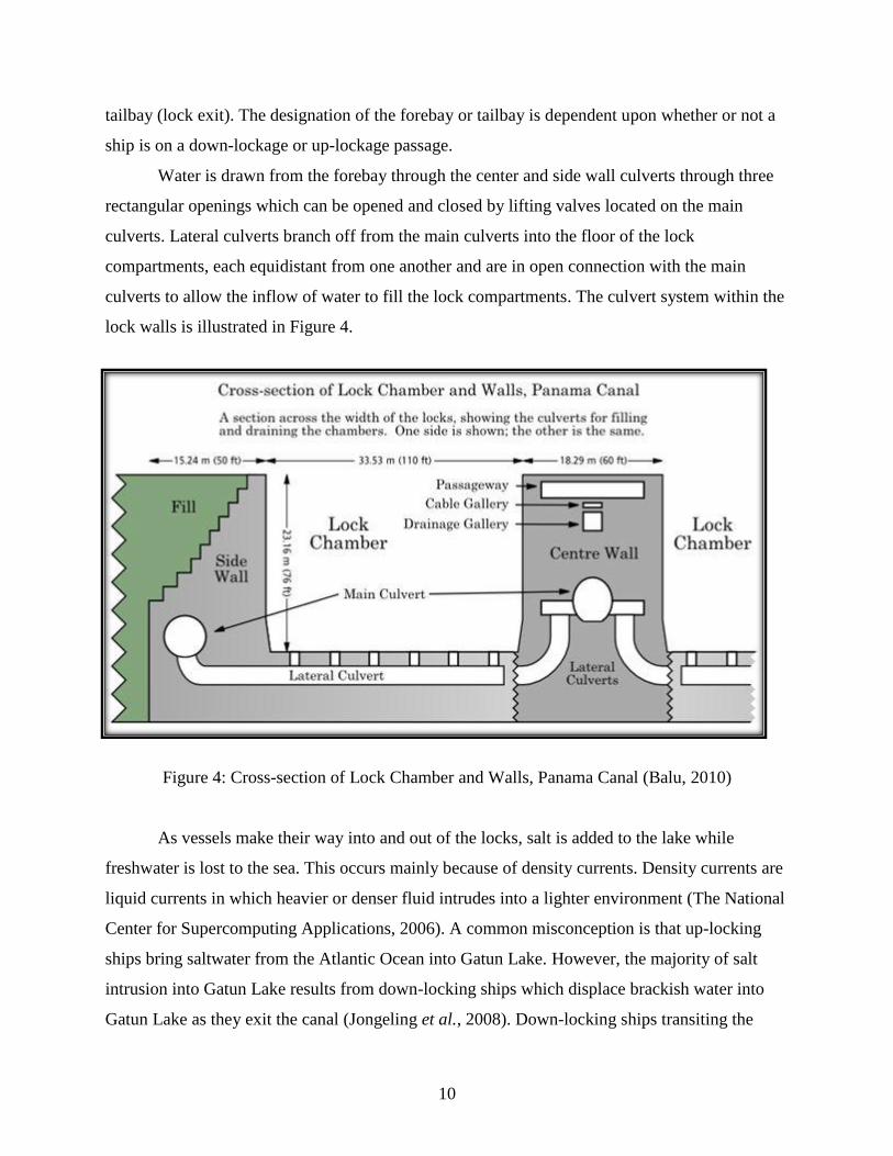
Water is drawn from the forebay through the center and side wall culverts through three

rectangular openings which can be opened and closed by lifting valves located on the main

culverts. Lateral culverts branch off from the main culverts into the floor of the lock

compartments, each equidistant from one another and are in open connection with the main

culverts to allow the inflow of water to fill the lock compartments. The culvert system within the

lock walls is illustrated in Figure 4.

Figure 4: Cross-section of Lock Chamber and Walls, Panama Canal (Balu, 2010)

As vessels make their way into and out of the locks, salt is added to the lake while

freshwater is lost to the sea. This occurs mainly because of density currents. Density currents are

liquid currents in which heavier or denser fluid intrudes into a lighter environment (The National

Center for Supercomputing Applications, 2006). A common misconception is that up-locking

ships bring saltwater from the Atlantic Ocean into Gatun Lake. However, the majority of salt

intrusion into Gatun Lake results from down-locking ships which displace brackish water into

Gatun Lake as they exit the canal (Jongeling et al., 2008). Down-locking ships transiting the

11

canal on the Atlantic side enter the Gatun Locks from Gatun Lake and make their way through

three lock compartments before exiting the canal into Limon Bay. Up-locking ships enter from

Limon Bay and pass through three locks compartments into Gatun Lake. Similar lock operations

occur on the Pacific side, the main difference being Miraflores Lake which is located between

the Pedro Miguel Locks and Miraflores Locks. The Miraflores Lake acts as a buffer to counteract

the saltwater displaced by transiting ships.

As a vessel sits in a lock compartment, the water on each side is separated by the lock

gate. When the gate opens, brackish water can enter the lake under the fresher water. As the

vessel travels down the three lock compartments, more and more brackish water can be displaced

into Gatun Lake. However, the salt that gets into Gatun Lake is diluted, creating a low salinity in

the lake (Jongeling et al., 2008).

Some of the contributing factors to salt exchange between locks are ship size, number of

daily passages of ships through locks, and variations in space and time of salt concentrations

close to the locks (DHI Water & Environment, 2005). With the current shipping schedule,

designated as the Gen3 shipping schedule, an average of 36 to 38 ships transits the canal every

day. Because larger ships displace a greater volume of water, the expansion project could

potentially increase salt intrusion into Gatun Lake. With the completion of the third set of locks,

a new shipping schedule called the PP1 will be implemented, allowing 12 Post-Panamax ships to

transit the canal per day.

Salt intrusion into and the loss of freshwater from Gatun Lake is of potential concern

because Gatun Lake is a source of drinking water for the local population. Gatun Lake , which

was formed nearly a century ago by the construction of the Gatun Dam, provides water for canal

operations, hydropower generation, and drinking water for the cities of Colón and Panama metro

area; the operational level of the lake is maintained to balance the water needs of these three

components (Fernandez & Schattanek, 2010). Nearly seven percent of the total available water in

Gatun Lake is used for public consumption, while 59% is used for canal operations and 34% of

the total available water is used for hydroelectric generation (Fernandez & Schattanek, 2010).

For use as drinking water, the lake supplies approximately 47 million gallons per day. The lake

loses about five million more gallons a day due to ship transit than it does supplying drinking

water to local communities (McAnally et al., 2000). The main focus is to keep the salinity of the

12

water at low levels during and after expansion so that Gatun Lake may continue to provide

drinking water to the populations of Panama metro area and Colón.

2.3.2 Impacts of Salt Intrusion

Although salt intrusion is not a current or foreseeable concern following the lock

expansion, the potential impact of salinity increases has been researched. Studies of Gatun Lake

have shown that increased salinity from salt intrusion, if it occurred, would adversely affect the

flora and fauna. URS Holdings, Inc. (2004) inventoried flora and fauna in Gatun Lake. They then

researched the impact increased salinity would have on the lake ecosystem and various species in

the lake. Plant species were divided into three groups: algae, aquatic macrophytes and

mangroves. A reported 147 species of six taxonomic groups were discovered for algae, 74

species of aquatic macrophytes, and 25 species of mangroves. 185 animal species were reported

within Gatun Lake and the Gatun locks. With regard to salinity impacts, URS Holdings, Inc

(2004) reported that only fifteen species may tolerate salinity levels of up to 1.32 ppt. Micro

algae as well as various fish, their larva and eggs could disappear completely from Gatun Lake

due to an increase in salt. This ultimately has an overall negative impact on the ecosystems in

Gatun Lake.

However, the Panama Canal Authority reports that the addition of the third set of locks

will not adversely affect the water quality in Gatun Lake:

“…the project will not cause permanent or irreversible impacts on water or air

quality…even when operating at maximum capacity, the third set of locks will not affect

the water quality of Gatun lake…the lake will keep its tropical fresh water quality with

stable ecosystems, and the water will be kept to well within appropriate quality levels and

standards in order that they can be made potable and used by the population” (Panama

Canal Authority, 2006b).

To confirm that salt levels are not increasing, the ACP monitors hydrometeorological parameters

that affect intruding salt into the lake and the lake water quality. This is done through routine

monitoring programs conducted by the ACP. The next chapter describes the ACP’s monitoring

programs.

13

3.0 Hydrometeorological and Water Quality Monitoring of Gatun Lake

ACP maintains many water quality and hydrometeorological measurement stations on the

rivers and the lakes within the Panama Canal Hydrographic Water basin area (La Cuenca

Hidrográfica del Canal de Panama or CHCP). The water quality measurement stations are sites

of interest designated by the ACP where in-situ data can be taken to indicate the water quality at

those particular locations. Data from these sites of interest are representative of the lake as a

whole. Since water quality measurement stations are just designated locations within the water

basin area, ACP personnel must travel to the sites in boats and acquire in-situ data using

equipment that measures water quality parameters. On the contrary, the hydrometeorological

measurement stations are equipped to measure hydrometeorological conditions in real-time.

Most stations are equipped to monitor conditions at regular time intervals; real-time data are

measured and archived every 15 seconds. In this way, data can be retrieved representing

measurements for longer time intervals such as hourly, daily, and yearly measurements. The

monitoring done by ACP at the measurement stations includes water quality parameters

(physical parameters such as temperature, conductivity, water column depth, and salinity) and

hydrometeorological conditions (such as air temperature, wind velocity, runoff, precipitation,

and evaporation). Each year the measurement data gathered by the stations are published by ACP

in hydrological and water quality year books (Jongeling et al., 2009). The following sections

describe the role of the water quality and hydrometeorological measurement stations in ACP’s

monitoring processes.

3.1 Water Quality Measurement Stations

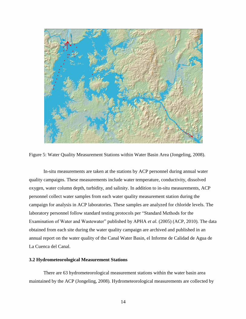
There are 68 water quality measurement stations within the water basin area: 21 sites

within the three reservoirs (Alhajuela, Gatun, and Miraflores); 8 sites within the main rivers; and

39 sites within other water bodies of the major sub-basins. Figure 5 shows the locations of the

water quality monitoring stations.

14

Figure 5: Water Quality Measurement Stations within Water Basin Area (Jongeling, 2008).

In-situ measurements are taken at the stations by ACP personnel during annual water

quality campaigns. These measurements include water temperature, conductivity, dissolved

oxygen, water column depth, turbidity, and salinity. In addition to in-situ measurements, ACP

personnel collect water samples from each water quality measurement station during the

campaign for analysis in ACP laboratories. These samples are analyzed for chloride levels. The

laboratory personnel follow standard testing protocols per “Standard Methods for the

Examination of Water and Wastewater” published by APHA et al. (2005) (ACP, 2010). The data

obtained from each site during the water quality campaign are archived and published in an

annual report on the water quality of the Canal Water Basin, el Informe de Calidad de Agua de

La Cuenca del Canal.

3.2 Hydrometeorological Measurement Stations

There are 63 hydrometeorological measurement stations within the water basin area

maintained by the ACP (Jongeling, 2008). Hydrometeorological measurements are collected by

15

the stations’s equipment every 15 seconds throughout each day of the year and are archived at

the measurement stations. The ACP monitors the hydrometeorological parameters of air

temperature, wind velocity, runoff, precipitation, and evaporation. Whereas most

hydrometeorological measurement stations are equipped to monitor only one or several of these

hydrometeorological parameters, some hydrometeorological stations, designated as “principal”

stations, measure all hydrometeorological parameters at their sites (Jongeling, 2008). The ACP

operates three principal hydrometeorological stations along the Panama Canal: Balboa Federal

Aviation Administration (FAA) station at the southern entrance of the canal (Pacific side),

Gamboa station at the mouth of Rio Chagres at the southern side of Gatun Lake, and Gatun

station at the northern side of the lake close to the shipping locks of the same name (Jongeling et

al., 2009). Table 1 shows the location of these stations in Universal Transverse Mercator (UTM)

coordinates as well as the elevation of each station given in Precise Level Datum (PLD) levels.

Table 1: ACP Hydrometeorological Stations

Station Latitude y

[UTM Zone 17N]

Longitude x

[UTM Zone 17N]

Elevation

Balboa FAA N 8.9689 ° 991664 W 79.5494 ° 659468 PLD + 10.1 m

Gamboa N 9.1122 ° 1007455 W 79.6939 ° 643528 PLD + 31.4 m

Gatun N 9.1122 ° 1024634 W 79.9206 ° 618565 PLD + 30.5 m

16

4.0 Salt Water Intrusion Modeling Software

Through its monitoring programs employed at the various water quality and

hydrometeorological measurement stations, the ACP has the capacity to record real-time

measurements and acquire information on the current conditions within the Panama Canal Water

Basin area. As the canal’s capacity and operations expand, it has become important for the ACP

to predict future conditions within the water basin. In particular, predicting water quality within

Gatun Lake is important to determine whether salinity levels may increase from increased canal

activity. While historical data can identify trends over long periods of time, modeling software is

used to predict future water quality in Gatun Lake and potentially avert any problems before they

occur. ACP currently utilizes Delft3D software for predictive modeling.

Delft3D software was developed by Deltares, a Dutch institute known for its

development of technology which analyzes delta processes and soft soil/sediment environments.

There have been four versions of the Delft3D software; the fourth was released on July 8, 2011

and is the first version based on open source code. This version of the software simulates the

hydrodynamics and inherent spatial characteristics of water systems.

As the name of the suite implies, Delft3D considers natural phenomena three-

dimensionally. The modeling suite of Delft3D is based on software that is continuously being

developed and approved through in-house research, development, and contributions by external

users of the system. Since natural processes are often time dependent and interrelated, Delft3D

simulates the interactions of water, sediment, and ecology in time and space to give an overall

water quality assessment. The suite is primarily used for the modeling of natural environments

such as coastal, river and estuarine areas. Delft3D has also been designed for integration into

more artificial environments, such as harbors and locks. The suite consists of a number of well-

tested and validated programs, which are linked to and are integrated with one another. Although

the software handles complex interactions, it is user-friendly and thus can be used by domain

experts and non-experts alike.

4.1 Delft3D-FLOW

Delft3D-FLOW is a multi-dimensional (2D or 3D) hydrodynamic simulation program.

This program calculates non-steady flow and transport phenomena resulting from tidal and

17

meteorological forcing on a rectilinear or curvilinear, boundary fitted grid. This program

includes the effect of density differences due to a non-uniform temperature and salinity

distribution (density-driven flow). The Delft3D-FLOW program has various areas of application

such as stratified and density driven flows, river flow simulation, simulations in deep lakes and

reservoirs, fresh-water river discharges in bays, and wave-driven currents. The area of

application that the project team focused on was salt intrusion and dispersion, specifically in

Gatun Lake.

Delft3D-FLOW can run simulations both in two-dimensional and three-dimensional

modes. The two-dimensional mode of Delft3D-FLOW, which models horizontal flow,

corresponds to solving depth-averaged equations. Tidal waves, storm surges, tsunamis, harbor

oscillations and transport of pollutants in vertically well-mixed flow regimes can be simulated by

Delft3D-FLOW in its two-dimensional mode using depth-averaged flow equations.

Transport problems where the horizontal flow significantly changes in the vertical

direction can be solved by three-dimensional modeling of Delft3D-FLOW. Changes in

horizontal flow may be caused by wind forcing, bed stress, Coriolis force, bed topography or

density differences. Examples in which the three-dimensional mode can be applied are

dispersion of waste or cooling water in lakes and coastal areas, salt intrusion in estuaries, fresh

water discharges in bays, and thermal stratification in lakes and seas.

Delft3D-RGFGRID, a part of Delft3D modeling suite, generates a curvilinear grid. A

curvilinear grid allows for a higher resolution in more important areas and lower resolution in

less important areas, which saves computational time. Three types of equations are used in

Delft3D-FLOW: horizontal equations of motion, the continuity equation, and transport equations

for conservative constituents. These equations are expressed in orthogonal curvilinear

coordinates or in spherical coordinates on the globe. The difference between curvilinear and

spherical coordinates is their plane of reference. Curvilinear coordinates’ free surface level and

bathymetry follow a flat horizontal plane of reference, whereas the spherical coordinates’

reference plane relates to the Earth’s curvature.

A special input file needs to be prepared to set up a Delft3D-FLOW model. Parameters

that are used for the input file depend on the physical phenomena being modeled, and on the

numerical techniques used for solving the equations that describe these phenomena. A Master

Definition File (MDF) is the input file that is used for storing the selected data of the model.

18

MDF files contain all the necessary data required for defining a model and running the

simulation program, such as temperature, discharges, wind, and evaporation data (Delft

Hydraulics, 2010).

While ACP was conducting water quality modeling studies in 2003 – 2005, Delft

Hydraulics was contracted by ACP to develop a simulation model tailored specifically to the

Panama Canal region. The new simulation model SWINLOCKS simulates and calculates the salt

load on Gatun Lake, Gaillard Cut and Miraflores Lake. The model can be used for the existing

locks and for Post-Panamax Locks in the future. The simulation model SWINLOCKS provides

an opportunity to compare the salt water load of different designs of Post-Panamax Locks. For

example, the model can be run to predict salt water loads for Post-Panamax Locks with or

without water saving basins, for the locks with or without salt water intrusion mitigation systems,

for various water control scenarios of Gatun Lake, and for different Post-Panamax ship traffic

intensities. Most importantly, a comparison of the salt load in the present situation to that of the

future situation can be drawn using this model. It also incorporates generalized shipping

schedules for the operation of the existing canal locks (Gen3) and for the operation of the future

canal locks (PP1). However, the simulation model SWINLOCKS is not capable of predicting the

time dependent salt water dispersion in Miraflores Lake, Gaillard Cut and Gatun Lake. For this

reason, the simulation model SWINLOCKS is run in parallel with Delft3D-Flow, which has the

capacity to analyze time-dependent variables (Jongeling et al., 2008).

4.2 Mass Balance

Within the hydrodynamic model Delft3D–FLOW, Gatun Lake is presented as a

hypothetical closed system with no open boundaries and the assumption that the total volume of

water is conserved within the lake. This virtual assumption is checked by a mass balance of the

real situation, considering all the relevant inflows and outflows of Gatun Lake. SWINLOCKS

does not consider the sources and sinks of Gatun Lake and only simulates the operation of the

locks and shipping schedules for lock transit; therefore, no mass balance is required to run the

SWINLOCKS model. The Delft3D-FLOW model can only be run when the mass balance

supports the assumption that the lake is a closed system. Understandably, it is expected that the

mass balance of the real-world Gatun Lake would not represent a perfectly closed system where

the difference between the lake inflows and outflows is zero. Namely, for the Gatun Lake

19

system, a mass balance which yields a water level difference of 1 m is the maximum acceptable

discrepancy for integration into the model. It is important that the lake system is closed when

implemented into the model since an unclosed system can produce unrealistic differences in the

water level of Gatun Lake. In addition, an unclosed lake system can imply that there are inflows

or outflows that are missing in the mass balance consideration which could affect water quality.

The mass balance indicates that the main sources of Gatun Lake’s inflow are rivers and the main

sources of outflow are both Gatun Dam and two locks systems (Gatun Locks and Pedro Miguel

Locks) (Jongeling et al., 2009).

4.3 Modeling Summary

The modeling capabilities of Delft3D software described in this chapter enable the ACP

to predict the future conditions of the canal water basin area. The saltwater intrusion and

dispersion calculation capacity of the SWINLOCKS simulation model was used by the project

team to forecast future salinity levels within the water basin area and in particular, within Gatun

Lake. The following chapter explains the methodology of the project team in determining how

hydrometeorological conditions affect salinity levels within Gatun Lake, which includes the

team’s use of the modeling software.

20

5.0 Methodology

The goals of this project were to (1) gather historical data describing hydrometeorological

characteristics of Gatun Lake, (2) model salt water intrusion through the Panama Canal and salt

water dispersion into Gatun Lake using hydrometeorological data, and (3) monitor current water

quality conditions through a water quality campaign. Historical hydrometeorological data from

2003 to 2005 and 2008 to 2009 were used as input for Delft3D hydrological modeling software

to obtain saltwater intrusion predictions. The team conducted a comparative analysis of the

model results from the two data sets. In a water quality campaign held by ACP, the team took

samples and obtained measurements for different water quality parameters (conductivity,

salinity, temperature and chlorides) at 68 locations in the lake. The model output from the

hydrometeorological data and the water quality in-situ data were compared to determine if

software simulations were representative of the current conditions in Gatun Lake. The following

sections explain the methods in more detail.

5.1 Historical Hydrometeorological Characteristics

The hydrometeorological section of El Departamiento del Ambiente, Agua, y Energia

(Environment, Water, & Energy Department) of the ACP provided the team with

hydrometeorological data from 2003 to 2005 and from 2008 to 2009. These data were used as

input data for salt intrusion modeling using Delft3D. Hydrometeorological data included the

hourly inflow and outflow rates of the Gatun Lake Watershed for every day from January 1,

2003 to December 31, 2005 and from January 1, 2008 to December 31, 2009. The data also

included hourly measurements for precipitation over the watershed, air temperature, wind

velocity and direction, atmospheric pressure, solar radiation, relative humidity, evaporation, and

elevations of Gatun and Madden Lake for every day over the two year period. ACP provided the

data to the team in Microsoft Excel files, which were then converted to text files in a script

recognizable by Delft3D.

5.2 Current Salt Intrusion Conditions

In order to assess current salt intrusion conditions in Gatun Lake, the team ran a saltwater

intrusion and dispersion simulation using Delft3D software (Scenario 0 – Current Conditions).

21

The D-FLOW program of Delft3D was used with water quality data from 2003 to 2005, which

was the most up-to-date data available to the team when Scenario 0 was run on November 14,

2011. Data from 2008 – 2009 were not obtained from ACP until the following day; this data still

needed to be organized before its use within the software. Prior analysis by the ACP had shown

that the conditions in Gatun Lake have remained consistent in recent history (ACP, 2010 &

Jongeling, 2008), thus the 2003 – 2005 data were deemed adequate. Scenario 0 used the Gen3

shipping schedule, a generalized schedule for shipping in the existing locks which describes the

current operation of the canal. It does not consider the future situation when the new set of locks

will be operating and a different shipping schedule will exist.

The water quality data acquired by the team during the water quality campaign (see

section 6.2) were compared to the results from Scenario 0 to demonstrate if the water quality in

Gatun Lake had changed over time. This comparison between historical data and current in-situ

data was completed to determine if factors other than operation of the new locks would

potentially affect salt intrusion in Gatun Lake.

5.3 Salt Intrusion Modeling

The team ran salt water intrusion and dispersion simulations using the

hydrometeorological data provided by the ACP for the two time periods of 2003 to 2005 and

2008 to 2009 using Delft 3D software. In particular, the D-FLOW program of Delft3D has the

capacity to run 5 scenarios within ACP’s contract with Deltares using the input

hydrometeorological data. Due to time constraints, the team ran one of the five scenarios.

Scenario 1 considered the operation of the canal after the expansion program is completed, using

the general Gatun Lake operating conditions and the water saving basins for the new locks. This

scenario utilizes general rules for operating the Gatun Dam and determines the yearly output

from Gatun Lake for the operation of the locks. Generalized shipping schedules for shipping in

the existing locks (shipping schedule Gen3) and for shipping in the future Post-Panamax Locks

(shipping schedule PP1) were used to determine how much salt intrusion will occur as a result of

the operation of the new locks. Since the existing locks will continue to be in use when the new

Post-Panamax locks are in operation, Scenario 1 considers a general schedule for each lock

system since the locks will be used concurrently. Thus, in each of the two simulation runs of

Scenario 1 (one for 2003 to 2005 and one for 2008 to 2009), salinity levels of Gatun Lake are

22

output considering the salt intrusion due to the operation of both series of locks (the existing

locks and Post-Panamax Locks)

5.4 Water Quality in Gatun Lake

As mentioned in Chapter 3, in order to monitor the water quality of Gatun Lake, ACP

conducts an annual water quality campaign in which it collects water samples from Gatun Lake

for measurements of various water quality parameters. Water quality measurement stations are

located at various sites throughout Gatun Lake. Over a 2-day period, the team visited 13 sites: 5

locations near Pedro Miguel Locks (PM14, PM15, PM17, PM20, and PM21) and 8 locations

near the Gatun Dam and Gatun Locks (Buoy D, P13, GL17, GE-1, GE-2, GE-3, P6, and Buoy

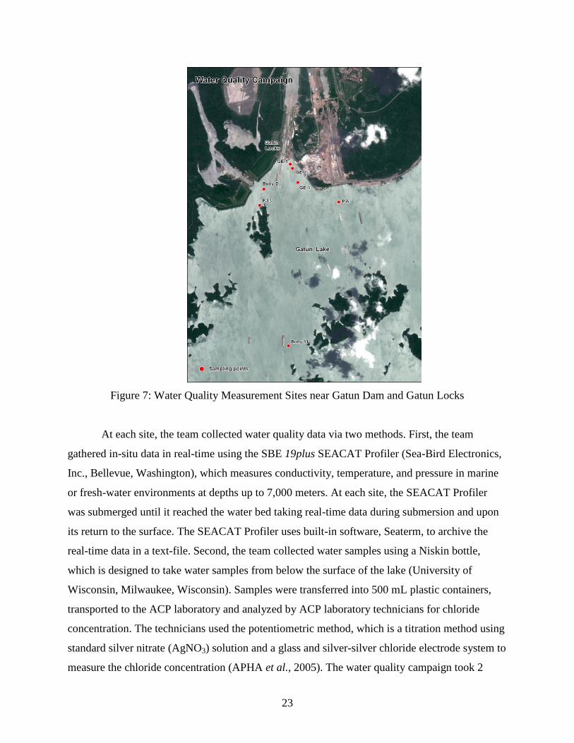
11). Figures 6 and 7 depict the sites the team visited; the locations of the sites are indicated in

each figure by blue dots and red dots, respectively.

Figure 6: Water Quality Measurement Sites near Pedro Miguel Locks

23

Figure 7: Water Quality Measurement Sites near Gatun Dam and Gatun Locks

At each site, the team collected water quality data via two methods. First, the team

gathered in-situ data in real-time using the SBE 19plus SEACAT Profiler (Sea-Bird Electronics,

Inc., Bellevue, Washington), which measures conductivity, temperature, and pressure in marine

or fresh-water environments at depths up to 7,000 meters. At each site, the SEACAT Profiler

was submerged until it reached the water bed taking real-time data during submersion and upon

its return to the surface. The SEACAT Profiler uses built-in software, Seaterm, to archive the

real-time data in a text-file. Second, the team collected water samples using a Niskin bottle,

which is designed to take water samples from below the surface of the lake (University of

Wisconsin, Milwaukee, Wisconsin). Samples were transferred into 500 mL plastic containers,

transported to the ACP laboratory and analyzed by ACP laboratory technicians for chloride

concentration. The technicians used the potentiometric method, which is a titration method using

standard silver nitrate (AgNO3) solution and a glass and silver-silver chloride electrode system to

measure the chloride concentration (APHA et al., 2005). The water quality campaign took 2

24

days. Due to time constraints, the team used data obtained from 3 of the 8 monitoring sites near

Gatun Dam and Gatun Locks for its analysis: Buoy D, GE-1, and P-6.

During this campaign, salinity levels at different depths of the water column for points

Buoy D, GE-1, and P-6 were generated by the Seaterm software. Depths were converted to

elevations by subtracting depths from the water surface elevation of Gatun Lake. For example,

the water surface elevation for Gatun Lake is 27 m (PLD), so for a salinity reading taken at a

depth of 5 m, the calculated elevation was 22 m (PLD).

25

6.0 Results and Analysis

The main goal of this project was to see how hydrometeorological conditions affect the

salinity levels in Gatun Lake. To meet this goal, the project team used historical

hydrometeorological data to predict salinity by software simulations and in-situ measurements

taken during its water quality campaign. The following sections explain the results acquired by

the team and the analysis of those results. Hydrometeorological input data for the software

simulations (Scenario 0 & 1) run by the team are presented and discussed in the first section. In

the following section, the salinity results from Scenario 0 run for 2003 to 2005 and the in-situ

salinity measurements from the water quality campaign are presented and compared. The last

section presents salinity results from Scenario 1 run for the two periods of 2003 to 2005 and

2008 to 2009. These results were analyzed to draw conclusions on how the operation of the

future Post-Panamax lock system would affect salinity levels in Gatun Lake.

6.1 Hydrometeorological Parameter Input Data for Software Simulations

To reach the main goal of the project, the team studied the variation of the

hydrometeorological parameters (air temperature, wind, precipitation, runoff, evaporation) in the

period of 2003-2005 and the period of 2008-2010. The Hydrometeorological Section of the ACP

provided data for each parameter. Each parameter represents a corresponding parameter built

into the Delft3D software used by the project team since each parameter affects the salinity

levels in Gatun Lake. As a result, the hydrometeorological data received from ACP by the

project team served as the input data for the saltwater intrusion and dispersion simulations

(Scenario 0 and Scenario 1) run by the software. The following sections present the input data

for each hydrometeorological parameter, and thus, each parameter of the software. Data were

monthly-averaged for each time period and compared to determine if hydrometeorological

conditions within Gatun Lake have remained consistent historically and throughout each time

period.

6.1.1 Air Temperature

Air temperature was one of the hydrometeorological parameters that was analyzed and

compared. As shown in Figure 8, 2003 has higher air temperature values than 2008, with a

26

difference of 0.5 – 1 degree. An exception can be observed from February to April of 2003,

where the highest air temperature value is 27.8 degrees, which is more than 2 degrees higher than

in 2008. Considering the second year of each data set, 2004 has significantly higher values in the

first quarter of the year than in 2009. In mid-February 2004 the temperature reached 27.6

degrees, while in March 2009 the temperature dropped down to almost 25 degrees Celsius. From

April to December, temperatures in 2004 and 2009 are similar. In 2010, the highest temperature

occurs in mid-April (28 degrees), which is 1 degree higher than in 2005. Then, while the air

temperature went up to 27.5 degrees from mid-May to mid-June in 2003, in 2005 the air

temperature dropped to 26.7 degrees during the same month period in 2005.

Figure 8: Air Temperature comparison 2003-2005, 2008-2010

6.1.2 Wind

As shown on Figure 9, there is a significant difference between the wind velocities of the

two time periods. Wind speeds in 2003 to 2005 are more than double the recorded values in 2008

to 2010. The wind velocity values for the years of 2003 – 2005 are approximately 2 to 6 m/s,

while the values for 2008 – 2010 are 0.7 – 4 m/s. The highest wind velocity values are observed

during the dry season (January-May) for the both time periods, with the values reaching 6 m/s

for 2003-2005 and 4 m/s for 2008-2010.

25

25.5

26

26.5

27

27.5

28

28.5

Mo

nth

- a

ver

aged

air

tem

per

aturt

e (©

)

Month

Air Temperature 2003-2005 Air Temperature 2008-2010

1st year 2nd year 3rd year

27

Figure 9: Wind velocity comparison 2003-2005, 2008-2010

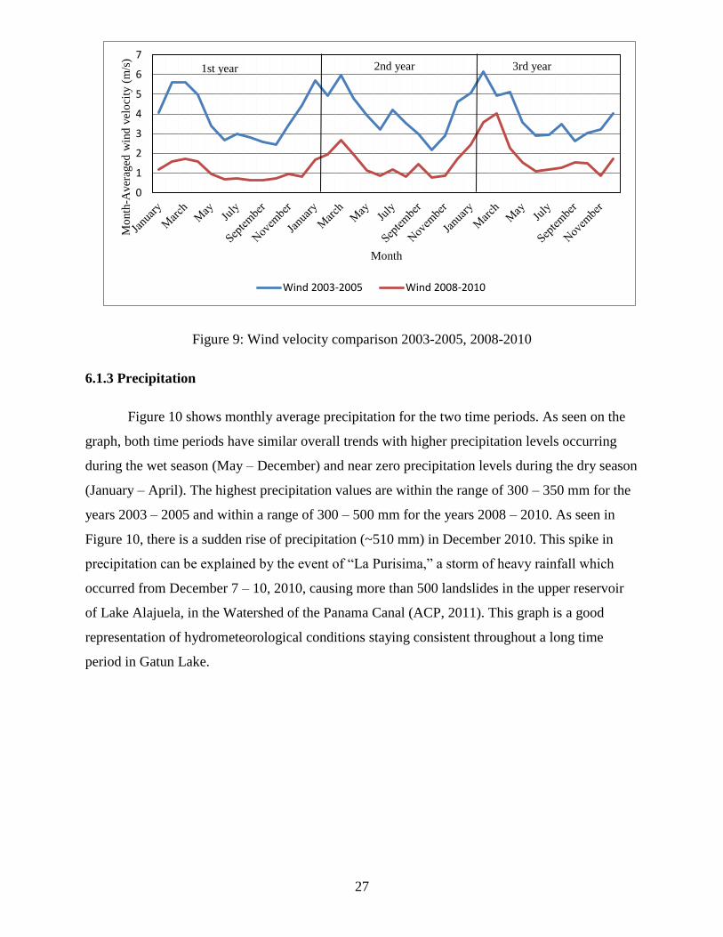
6.1.3 Precipitation

Figure 10 shows monthly average precipitation for the two time periods. As seen on the

graph, both time periods have similar overall trends with higher precipitation levels occurring

during the wet season (May – December) and near zero precipitation levels during the dry season

(January – April). The highest precipitation values are within the range of 300 – 350 mm for the

years 2003 – 2005 and within a range of 300 – 500 mm for the years 2008 – 2010. As seen in

Figure 10, there is a sudden rise of precipitation (~510 mm) in December 2010. This spike in

precipitation can be explained by the event of “La Purisima,” a storm of heavy rainfall which

occurred from December 7 – 10, 2010, causing more than 500 landslides in the upper reservoir

of Lake Alajuela, in the Watershed of the Panama Canal (ACP, 2011). This graph is a good

representation of hydrometeorological conditions staying consistent throughout a long time

period in Gatun Lake.

0

1

2

3

4

5

6

7

Mo

nth

-Aver

aged

win

d v

elo

city

(m

/s)

Month

Wind 2003-2005 Wind 2008-2010

2nd year 3rd year 1st year

28

Figure 10: Precipitation comparison 2003-2005, 2008-2010

6.1.4 Runoff

For this parameter, discharges of three principal rivers were used. These principal rivers

are Rio Ciri Grande, Rio Gatun, and Rio Trinidad. As shown in Figure 11, the patterns stay

nearly consistent for each of the rivers. All three rivers have their highest peaks during the

months of September to December which are the months of the rainy season. Precipitation is one

of the conditions that directly affect the discharge values.

Rio Trinidad has a major difference in discharge of 10 m3/s between mid-November

values in 2003 and mid-November values in 2008. The river discharges in the years of 2004 and

2009 are similar. The year 2010 has a sudden peak of 27 m3/s in mid-December as does Rio Ciri

Grande, which is due to the storm “La Purisima” (ACP, 2011). This value is higher by 20 m3/s

than the mid-December value of 2005, which is a very significant difference throughout the

overall trend.

0

100

200

300

400

500

600

Mo

nth

-aver

aged

pre

cip

itat

ion (

mm

)

Month

Precipitation 2003 - 2005 Precipitation 2008 - 2010

1st year 3rd year 2nd year

29

Figure 11: Runoff comparison for three principal rivers 2003-2005, 2008-2010

05

101520253035404550

Mo

nth

-aver

aged

dis

char

ge

(m3

/s)

Month

Rio Ciri Grande 2003-2005 Rio Ciri Grande 2008-2010

2nd year 3rd year 1st year

0

5

10

15

20

25

30

Mo

nth

-aver

aged

dis

char

ge

(m3

/s)

Month

Rio Gatun 2003-2005 Rio Gatun 2008-2010

3rd year 2nd year

0

5

10

15

20

25

30

Mo

nth

-aver

aged

dis

char

ge

(m3

/s)

Month

Rio Trinidad 2003-2005 Rio Trinidad 2008-2010

2nd year 3rd year 1st year

30

For Rio Gatun, similar patterns are observed from January to mid–June for 2003 and

2008. In 2008, the peak value of 12 m3/s is observed in mid-July, which is 5 m

3/s higher than the

discharge rate in 2003. Also, while the highest peak discharge occurred in mid-December in

2003, in 2008 it occurred in mid-November. The years 2004 and 2009 have very similar patterns

except for a 4 m3/s difference in the first half of April. Mid-June of 2010 has a peak discharge of

approximately 10 m3/s, which is almost 8 m

3/s higher than in the year 2005. However, both years

have the same peak of 15 m3/s in mid-November.

For Rio Ciri Grande, both time periods have very similar ranges of monthly averaged

discharge. However, as shown in Figure 11, mid-October of 2003 has a peak discharge value of

28 m3/s, which is approximately 5 m

3/s greater than in the year 2008. That is the most significant

difference for Rio Ciri Grande, except for a sudden rise in December 2010 due to “La Purisima”.

6.1.5 Evaporation

Figure 12 shows that there is a significant difference in evaporation values for the two

time periods. The evaporation values for 2003 to 2005 are within a range of 390 to 950 mm/day.

For the 2008 to 2010 time frame, evaporation ranges from 190 to 400 mm/day. The decrease in

evaporation values in recent years may be due to increased cloud coverage during the years of

2008 – 2010 or to increased solar radiation during the years of 2003 – 2005.

Figure 12: Evaporation comparison 2003-2005, 2008-2010

0

200

400

600

800

1000

1200

Mo

nth

-aver

aged

evap

ora

tio

n

(mm

/day

)

Month Evaporation 2003-2005 Evaporation 2008-2010

1st year 2nd year 3rd year

31

6.2 Water Quality Campaign Results and Simulation Results for Scenario 0

The hydrometeorological input data from the period 2003 to 2005, as presented in the

previous section, were run within Scenario 0 of the software. As explained in Chapter 5,

Scenario 0 was a simulation which used a generalized schedule (Gen3) for shipping in the

existing lock system to describe the current operation of the canal. Consequently, the simulation

does not consider the future situation when the new set of locks (Post-Panamax) will be

operating and a different shipping schedule will exist. The purpose of running Scenario 0 was to

determine if the software simulations were representative of the real conditions in Gatun Lake.

To this end, the project team compared the simulation salinity results from Scenario 0 to real in-

situ salinity measurements taken by the team during its water quality campaign. This section

presents the in-situ salinity measurements taken at different water quality measurement stations

during the water quality campaign and draws comparisons between these measurements and the

salinity results from the software for Scenario 0.

During the water quality campaign, salinity measurements were collected at 13 sites near

Pedro Miguel and Gatun Locks. Due to time constraints, the data from 3 stations near the Gatun

Locks were analyzed by the team. Figure 13 displays the locations of the three measuring sites

that were chosen: BuoyD, GE-1, and P-6.

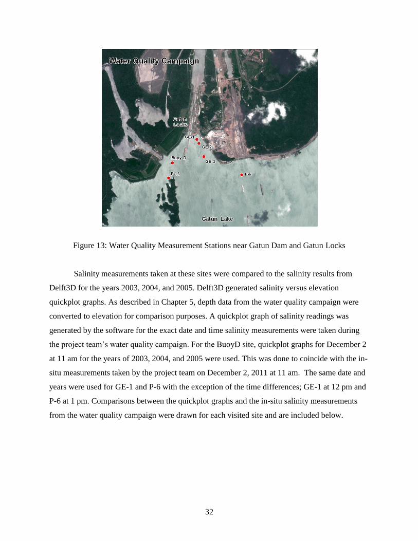
32

Figure 13: Water Quality Measurement Stations near Gatun Dam and Gatun Locks

Salinity measurements taken at these sites were compared to the salinity results from

Delft3D for the years 2003, 2004, and 2005. Delft3D generated salinity versus elevation

quickplot graphs. As described in Chapter 5, depth data from the water quality campaign were

converted to elevation for comparison purposes. A quickplot graph of salinity readings was

generated by the software for the exact date and time salinity measurements were taken during

the project team’s water quality campaign. For the BuoyD site, quickplot graphs for December 2

at 11 am for the years of 2003, 2004, and 2005 were used. This was done to coincide with the in-

situ measurements taken by the project team on December 2, 2011 at 11 am. The same date and

years were used for GE-1 and P-6 with the exception of the time differences; GE-1 at 12 pm and

P-6 at 1 pm. Comparisons between the quickplot graphs and the in-situ salinity measurements

from the water quality campaign were drawn for each visited site and are included below.

33

6.2.1 BuoyD

Salinity measurements from the water quality campaign at BouyD are shown in Figure

14, while simulated salinity levels per the Delft3D software for 2003, 2004 and 2005 are shown

in Figure 15. The model results show similar trends to the measured values.

Figure 14: Delft3D Quickplot Salinity Modeling Results at BuoyD for 2003-2005

Figure 15: Salinity Measurements at BuoyD on December 2, 2011 at 11 am

0

5

10

15

20

25

30

0.000 0.020 0.040 0.060 0.080 0.100 0.120 0.140 0.160

Ele

vat

ion (

m)

Salinity (ppt)

34

The salinity values are reasonably consistent from the surface to an elevation of

approximately 5 meters. Below 5 meters, the salinity levels increase. However, the salinity levels

remain within the acceptable range for freshwater lakes (less than 0.5 ppt) at all elevations in the

model and in the measurements. The salinity increase in the bottom layers of the lake is likely

due to the location of BuoyD. As shown in Figure 13, the BuoyD station is located right in front

of the Gatun Locks where incoming salt through the locks gets accumulated. High salinity

currents from the locks cause the sudden increase in salinity in the bottom layers of the lake.

6.2.2 GE-1

Salinity measurements from the water quality campaign at GE-1 are shown in Figure 16,

while simulated salinity levels per the Delft3D software for 2003, 2004 and 2005 are shown in

Figure 17

Figure 16: Quickplot Salinity Modeling Results at GE-1 for 2003-2005

35

Figure 17: Salinity Measurements at GE-1 on December 2, 2011 at 12 pm

As seen in Figure 17, there is no consistent pattern for salinity at the different elevations

of GE-1, which is likely due to the location of the station. As Figure 13 shows, the GE-1

measuring station is located to the right of the locks where there is high turbulence from the

ships and boats going through the locks. The salinity values for the quickplot graphs of GE-1 are

very close to the values of BuoyD since both stations are located close to the locks (Figure 14 &

16). There is a minor difference in salinity between the measured values from the water quality

campaign and the quickplot graphs for the years of 2003 and 2004 (0.02-0.03ppt). The quickplot

for the year 2005 has salinity values around 0.1 ppt, which is higher than the rest of the graphs.

Still, these graphs are representative of salinity over a very short time period, whereas long-term

patterns would be more consistent with the modeling results from the Delft3D.

6.2.3 P-6

Salinity measurements from the water quality campaign at P-6 are shown in Figure 18,

while simulated salinity levels per the Delft3D software for 2003, 2004 and 2005 are shown in

Figure 19. Measured values during the water quality campaign showed salinity at P-6 to be 0.05

– 0.06 that are within the acceptable range of salinity in fresh water (> 0.5 ppt). The salinity

levels for the quickplot graphs are consistent during the years of 2003 and 2004 with salinity

measurements ranging from 0.066 to 0.071 ppt. The values of 2005 are higher by 0.03 – 0.04

ppt than the values of the previous two years.

10

12

14

16

18

20

22

24

26

28

0.0532 0.0533 0.0534 0.0535 0.0536 0.0537 0.0538 0.0539

Ele

vat

ion (

m)

Salinity (ppt)

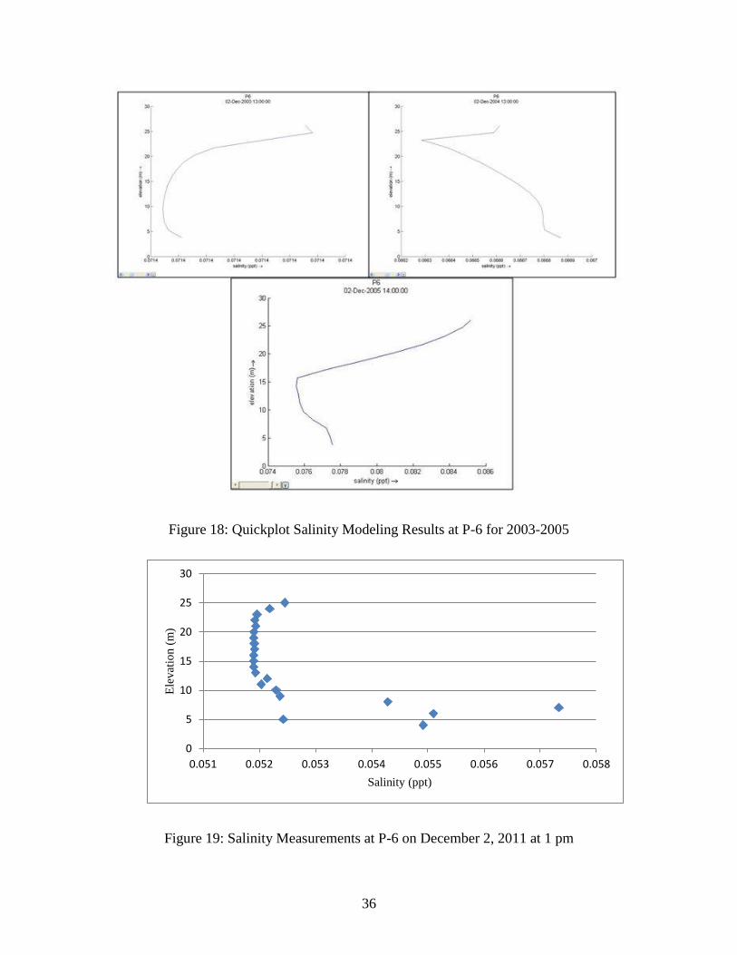
36

Figure 18: Quickplot Salinity Modeling Results at P-6 for 2003-2005

Figure 19: Salinity Measurements at P-6 on December 2, 2011 at 1 pm

0

5

10

15

20

25

30

0.051 0.052 0.053 0.054 0.055 0.056 0.057 0.058

Ele

vat

ion (

m)

Salinity (ppt)

37

The salinity results from the software simulation for Scenario 0 were consistent with the

in-situ measurements of the water quality campaign. This demonstrates that the software is

working correctly and is representative of the real conditions in the lake, and that the conditions

of Gatun Lake have remained consistent over time, up to the present-day. In addition, since

Scenario 0 only considers the operation of the current lock system, the consistency between the

software results and the in-situ measurements implies that only the operation of the new locks

would potentially affect salt intrusion in Gatun Lake and other factors will not affect predicted

lake water quality.

6.3 Salinity Results for Scenario 1

The hydrometeorological input data from the periods 2003 to 2005 and 2008 to 2009, as

presented in the Section 6.1, were run using the software for Scenario 1. As explained in

Chapter 5, one run was done for each time period for a total of two runs. Scenario 1 includes

both the the generalized schedule (Gen3) for shipping in the existing lock system and a

generalized shipping schedule, PP1, for the future Post-Panamax locks. Thus, the salinity results

generated by the software for Scenario 1 represent the future conditions in Gatun Lake when

both series of locks are in operation. This section presents the salinity results for five freshwater

intake stations, Sabanitas, Mt Hope, Escobal, Gamboa, and Paraiso, from the software for the

each run of Scenario 1.

Although the five freshwater intake stations are far from the Gatun shipping locks (see

Figure 20), special attention is given to them because these five points are freshwater intake

stations for drinking water. Therefore, monitoring salinity levels at these locations is of high

importance. Graphs were prepared for the bottom as well as the surface water elevations to

illustrate salt concentrations at both extremes. Typically, the highest salt concentration at a

specific point lies at the bottom of the lake while the lowest salt concentration occurs at the

lake’s surface.

38

Figure 20: Freshwater Intake Stations in Gatun Lake

In addition, to gain a better understanding of the salt intrusion phenomena near the Gatun

shipping locks, the team averaged the salinity levels for 23 hydrometeorological stations located

throughout Gatun Lake. The team made a graph of the salinity level average from these 23 points

as a representation of the overall salinity in Gatun Lake. The following sections display salinity

graphs for various locations throughout Gatun Lake as well as a salinity graph for Gatun Lake as

a whole (as the average of the salinity levels at the 23 sites). The salinity results displayed in

these graphs are indicative of the future salinity levels at the five freshwater intake stations and

in Gatun Lake in whole as a result of operating the current lock system with the future Post-

Panamax lock system. Each graph was produced from simulation salinity results for Scenario 1.

6.3.1 Sabanitas

Figures 21 and 22 illustrate that the volume-averaged salinities at the bottom and surface

of Sabanitas over the two time periods (2003-2005 and 2008-2009) are very similar and their

differences in salt levels are insignificant. The volume-averaged salinities vary between about

39

0

0.05

0.1

0.15

0.2

0.25

0.3

Q1 Q2 Q3 Q4 Q1 Q2 Q3 Q4 Q1 Q2 Q3 Q4

20032008

20042009

2005

Sal

init

y (

pp

t)

Quarter Annual Periods

2003-2005

2008-2009

0

0.05

0.1

0.15

0.2

0.25

0.3

Q1 Q2 Q3 Q4 Q1 Q2 Q3 Q4 Q1 Q2 Q3 Q4

20032008

20042009

2005

Sal

init

y (

pp

t)

Quarter Annual Periods

2003-2005

2008-2009

0.1 ppt and 0.17 ppt. This range of salinity in the years 2008 and 2009 is very low and is

consistent with the years 2003-2005.

Figure 21: Sabanitas Salt Concentration at Depth 1 m above Bottom

Figure 22: Sabanitas Salt Concentration at Depth 1 m below Surface

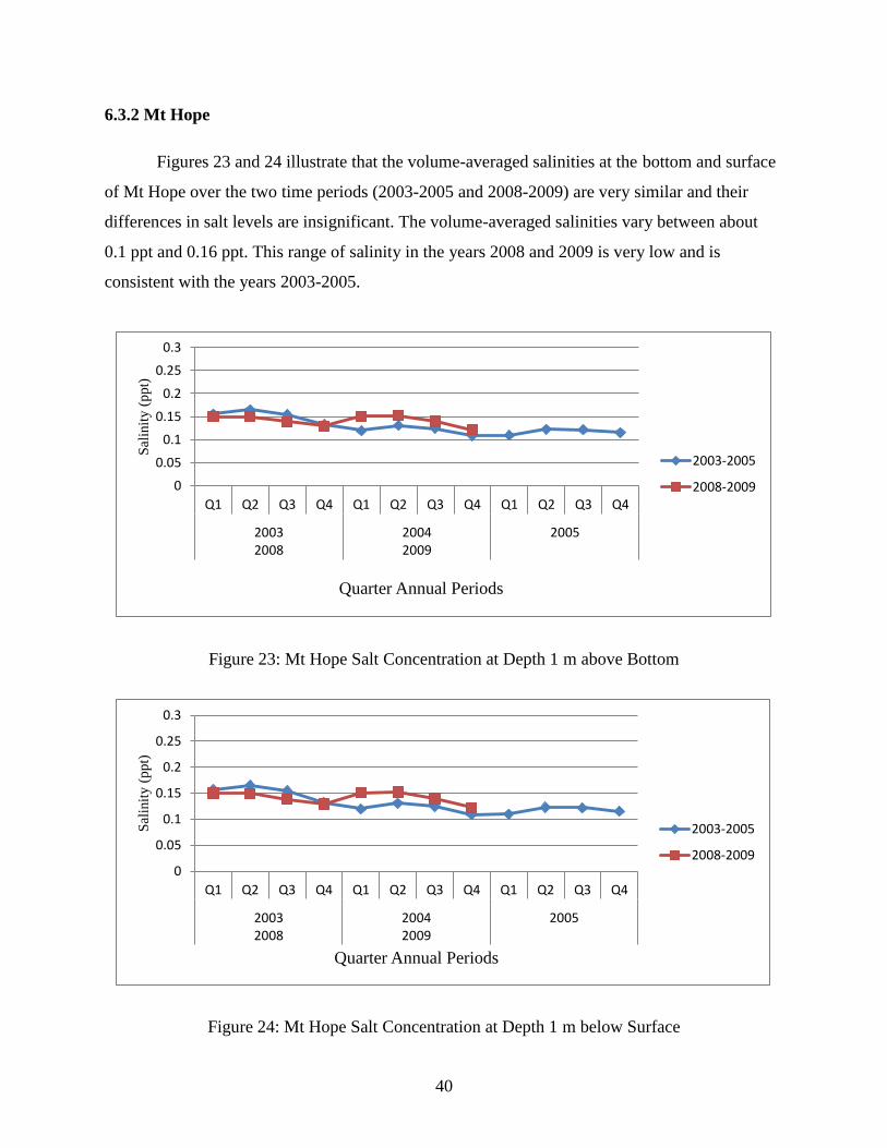
40

0

0.05

0.1

0.15

0.2

0.25

0.3

Q1 Q2 Q3 Q4 Q1 Q2 Q3 Q4 Q1 Q2 Q3 Q4

20032008

20042009

2005

Sal

init

y (

pp

t)

Quarter Annual Periods

2003-2005

2008-2009

0

0.05

0.1

0.15

0.2

0.25

0.3

Q1 Q2 Q3 Q4 Q1 Q2 Q3 Q4 Q1 Q2 Q3 Q4

20032008

20042009

2005

Sal

init

y (

pp

t)

Quarter Annual Periods

2003-2005

2008-2009

6.3.2 Mt Hope

Figures 23 and 24 illustrate that the volume-averaged salinities at the bottom and surface

of Mt Hope over the two time periods (2003-2005 and 2008-2009) are very similar and their

differences in salt levels are insignificant. The volume-averaged salinities vary between about

0.1 ppt and 0.16 ppt. This range of salinity in the years 2008 and 2009 is very low and is

consistent with the years 2003-2005.

Figure 23: Mt Hope Salt Concentration at Depth 1 m above Bottom

Figure 24: Mt Hope Salt Concentration at Depth 1 m below Surface

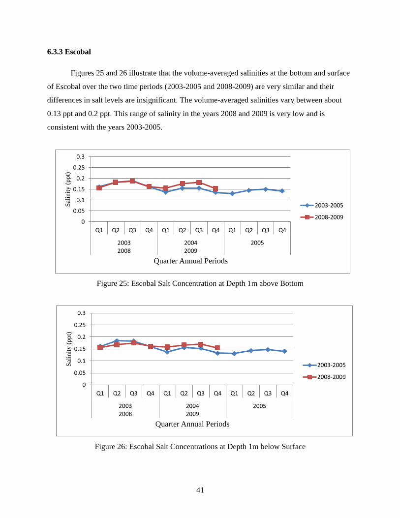
41

6.3.3 Escobal

Figures 25 and 26 illustrate that the volume-averaged salinities at the bottom and surface

of Escobal over the two time periods (2003-2005 and 2008-2009) are very similar and their

differences in salt levels are insignificant. The volume-averaged salinities vary between about

0.13 ppt and 0.2 ppt. This range of salinity in the years 2008 and 2009 is very low and is

consistent with the years 2003-2005.

Figure 25: Escobal Salt Concentration at Depth 1m above Bottom

Figure 26: Escobal Salt Concentrations at Depth 1m below Surface

0

0.05

0.1

0.15

0.2

0.25

0.3

Q1 Q2 Q3 Q4 Q1 Q2 Q3 Q4 Q1 Q2 Q3 Q4

20032008

20042009

2005

Sal

init

y (

pp

t)

Quarter Annual Periods

2003-2005

2008-2009

0

0.05

0.1

0.15

0.2

0.25

0.3

Q1 Q2 Q3 Q4 Q1 Q2 Q3 Q4 Q1 Q2 Q3 Q4

20032008

20042009

2005

Sal

init

y (

pp

t)

Quarter Annual Periods

2003-2005

2008-2009

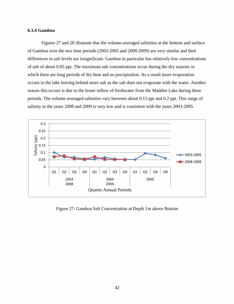
42

6.3.4 Gamboa

Figures 27 and 28 illustrate that the volume-averaged salinities at the bottom and surface

of Gamboa over the two time periods (2003-2005 and 2008-2009) are very similar and their

differences in salt levels are insignificant. Gamboa in particular has relatively low concentrations

of salt of about 0.05 ppt. The maximum salt concentrations occur during the dry seasons in

which there are long periods of dry heat and no precipitation. As a result more evaporation

occurs in the lake leaving behind more salt as the salt does not evaporate with the water. Another

reason this occurs is due to the lesser inflow of freshwater from the Madden Lake during these

periods. The volume-averaged salinities vary between about 0.13 ppt and 0.2 ppt. This range of

salinity in the years 2008 and 2009 is very low and is consistent with the years 2003-2005.

Figure 27: Gamboa Salt Concentration at Depth 1m above Bottom

0

0.05

0.1

0.15

0.2

0.25

0.3

Q1 Q2 Q3 Q4 Q1 Q2 Q3 Q4 Q1 Q2 Q3 Q4

20032008

20042009

2005

Sal

init

y (

pp

t)

Quarter Annual Periods

2003-2005

2008-2009

43

Figure 28: Gamboa Salt Concentration at Depth 1m below Surface

6.3.5 Paraiso

Figures 29 and 30 illustrate that the volume-averaged salinities at the bottom and surface

of Paraiso over the two time periods (2003-2005 and 2008-2009). The volume-averaged

salinities vary between about 0.15 ppt and 0.275 ppt and vary more significantly than at other

freshwater intake stations. The salinity values presented here are also the highest of any station.

This occurs mainly because the Paraiso water intake station is directly influenced by the Pacific

Locks as it is located in close proximity to the Pedro Miguel Locks where the highest

concentration of salt occurs. Although the results at this freshwater intake station vary more than

others and are more elevated, the salinity levels present no concern as they are well below 0.5

ppt.

0

0.05

0.1

0.15

0.2

0.25

0.3

Q1 Q2 Q3 Q4 Q1 Q2 Q3 Q4 Q1 Q2 Q3 Q4

20032008

20042009

2005

Sal

init

y (

pp

t)

Quarter Annual Periods

2003-2005

2008-2009

44

Figure 29: Paraiso Salt Concentration at Depth 1m above Bottom

Figure 30: Paraiso Salt Concentration at Depth 1 m below Surface

6.3.6 Gatun Lake

As seen in Figure 31 the salt concentrations throughout the two time periods (2003-2005

and 2008-2009) are very consistent. The salinity ranges between 0.13 ppt and 0.2 ppt. The

0

0.05

0.1

0.15

0.2

0.25

0.3

Q1 Q2 Q3 Q4 Q1 Q2 Q3 Q4 Q1 Q2 Q3 Q4

20032008

20042009

2005

Sal

init

y (

pp

t)

Quarter Annual Periods

2003-2005

2008-2009

0

0.05

0.1

0.15

0.2

0.25

0.3

Q1 Q2 Q3 Q4 Q1 Q2 Q3 Q4 Q1 Q2 Q3 Q4

20032008

20042009

2005

Sal

init

y (

pp

t)

Quarter Annual Periods

2003-2005

2008-2009

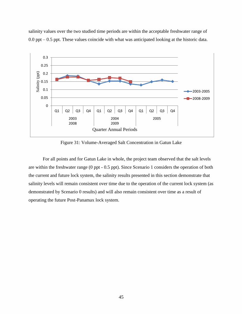
45

salinity values over the two studied time periods are within the acceptable freshwater range of

0.0 ppt – 0.5 ppt. These values coincide with what was anticipated looking at the historic data.

Figure 31: Volume-Averaged Salt Concentration in Gatun Lake

For all points and for Gatun Lake in whole, the project team observed that the salt levels

are within the freshwater range (0 ppt - 0.5 ppt). Since Scenario 1 considers the operation of both

the current and future lock system, the salinity results presented in this section demonstrate that

salinity levels will remain consistent over time due to the operation of the current lock system (as

demonstrated by Scenario 0 results) and will also remain consistent over time as a result of

operating the future Post-Panamax lock system.

0

0.05

0.1

0.15

0.2

0.25

0.3

Q1 Q2 Q3 Q4 Q1 Q2 Q3 Q4 Q1 Q2 Q3 Q4

20032008

20042009

2005

Sal

init

y (

pp

t)

Quarter Annual Periods

2003-2005

2008-2009

46

7.0 Water Treatment Plant

Delft3D modeling results showed that salt levels within Gatun Lake have remained

consistent and are predicted to stay within the freshwater range, with salt levels less than 0.5 ppt.

However, it is still possible that modeling efforts have not fully captured future water quality

scenarios, or that changes in shipping schedules or operation of the locks could result in

increased salt levels in Gatun Lake after the expansion project is completed. In order to prepare

for these possible situations, the project team designed a water treatment facility that produces

potable water for the city of Colon and the Panama City metro area considering brackish water

conditions in Gatun Lake.

7.1 Plant Specifications

Gatun Lake supplies the populations of the Panama City metro area and the city of Colon

with an estimated 115 MGD of water through three water treatment facilities. The Miraflores

filtration plant is located on the Pacific side (45 MGD), and on the Atlantic side there is the

Mount Hope filtration plant (42 MGD) and the Sabanitas filtration plant (28 MGD). The 2010

populations for the Panama City metro area and Colon are estimated at 1.207 million and

242,000, respectively (Hubbard, 2012). According to the CIA World Fact Book (2012), Panama

experiences a population growth rate of 1.435% annually. Given the populations and annual

growth rate, the 2032 populations of the Panama City metro area and Colon are an estimated

1.588 million and 318,000, respectively. Using a relative ratio of the 2010 populations and water

demands to the projected 2032 populations, the water demand through 2032 is estimated to be

150 MGD.

Panamanian law requires that drinking water discharges comply with COPANIT 23-395-

99 which states that treatment of surface waters requires some form of flocculation, coagulation,

sedimentation, or filtration in addition to disinfection. Specific information on processes at the

current water filtration plants was not available. A summary of important raw water quality

conditions are listed in Table 2.

47

Table 2: Raw Water Quality in Gatun Lake (ACP, 2010)

Parameter Average Value

Turbidity (NTU) 35.2

Dissolved Oxygen (mg/L) 6.06

pH 7.32

Conductivity (µS/cm) 148

Salinity (ppt) 0.5

Chlorine (mg/L) 8.3

Total Dissolved Solids (mg/L) 96

Total Suspended Solid (mg/L) 31

Alkalinity (mg/L CaCO3) 52

N-NO2 (mg/L) 0.001

N-NO3 (mg/L) 0.198

P-PO4 (mg/L) 0.010

SO4 (mg/L) 3.2

Hardness (mg/L CaCO3) 51.7

E. coli (MPN/100 mL) 64

Total Coliforms (MPN/100 mL) 2857

The project team assumed the same raw water quality as currently in the lake for the

design of the plant, with the exception of increased salt. Brackish water is defined as water

containing salt levels within the range of 0.5 ppt to 30 ppt. Any value above 30 ppt is considered

salt water and any value below 0.5 ppt is considered freshwater. Due to the unlikelihood that the

salt levels within Gatun Lake would reach 30 ppt, the team considered a lower value between 0.5

ppt and 15 ppt.

7.2 Design Alternatives

Treatment of brackish waters to drinking water standards (including a salt level less than

0.5 ppt) can be accomplished using membranes. The different types of membranes available are

shown in Table 3. Microfiltration and ultrafiltration do not reject salt and are therefore not

applicable for brackish waters. For this reason, microfiltration and ultrafiltration are not

48

discussed further. While nanofiltration aids in the removal of salt by softening the water, the

technology is not sufficient on its own to remove salt from water. Two technologies for salt

removal that were examined are electrodialysis reversal and reverse osmosis.

Table 3: Membrane Types

Membrane Driving force Membrane

Structure

Applications

Microfiltration Pressure Macropores Pretreatment for NF and RO;

particle, cyst, and bacterial

removal

Ultrafiltration Pressure Mesopores Pretreatment for NF and RO;

macromolecule, cyst, bacteria,

and virus removal

Nanofiltration Pressure Micropores Softening; NOM removal

Reverse osmosis Pressure Dense, or thin film

composite

Demineralization; TDS

reduction, brackish and

seawater desalinization

Electrodialysis

Reversal

Electrical

potential and

pressure

Ion exchange Brackish water desalinization

7.2.1 Electrodialysis and Electrodialysis Reversal

Electrodialysis (ED) is a membrane treatment processes that was developed in the 1950s.

This process uses an electrical potential to remove salts and other ions through ion selective

membranes to a concentrate collecting stream. The principal application of ED for water

treatment is the desalination of brackish water.

Electrodialysis uses a configuration called an electrodialysis cell that consists of two

compartments (dilute and brine) that are formed by an anion exchange membrane and a cation

exchange membrane placed between two electrodes. Usually, multiple ED cells are arranged into

a stack to provide a higher salt removal percentage. Anion and cation exchange membranes get

arranged alternatively to form the multiple electrodialysis cell. ED cells separate the solution

with anion exchange membranes, permeable only for anions and cation exchange membranes,

permeable only for cations.

49

As shown in Figure 32, the stack of multiple ED cells has three different types of streams

going through it. These streams are the dilute (D) feed stream, brine (C) stream, and electrode

(E) stream. There are also an anode and cathode on two sides of the of ED stack. The anode and

cathode are electrodes that have an electric current from a polarized electrical device flowing

through them. Anions, negatively charged ions, migrate towards the positively charged anode

because of an electrical potential difference. Anions pass through the positively charged ion

exchange membrane, but they get stopped in the (C) stream when reaching the negatively

charged ion exchange membrane, which results in (C) stream becoming highly concentrated with

anions. The opposite happens to cations, which are positively charged ions. When they move

towards the negatively charged cathode, they pass through the negatively charged ion exchange

membrane and get stopped by the positively charged ion exchange membrane and also stay in

the (C) stream. Electric current flows between the cathode and anode because of the anion and

cation migration. As a result of the electrodialysis process, the (C) stream ends up highly

concentrated with ions, while the ion concentration in the (D) stream dramatically decreases. The

(E) stream flows past each electrode in the stack and it can have the same or different species as

the feed stream passing through it.

Figure 32: Electrodialysis Process (EET Corporation, 2009)

50

Electrodialysis reversal (EDR) uses the same concept as electrodialysis, except the

polarity charges on the membrane get periodically changed, which causes the flow to reverse. It

is done to reduce fouling and to extend the membrane life.

Typical removal of salt from brackish water ranges from 25 to 40 percent of dissolved

solids per stage of treatment. Therefore, efficient removal of salt by ED requires multiple stage

treatment systems. With every additional stage the salt percent removal increases by 25 – 30

percent. Figure 33 shows a schematic of a three-stage EDR process with four treatment trains,

which has 90% overall recovery and 87.5% solute removal (Trussell Technologies, 2008).

Figure 33: EDR configuration (Trussell Technologies, 2008)

The energy requirement for ED systems is 2.6 – 4.2 kWh/1,000 gallons of product water

for removal of 300 mg/L of dissolved solids. In addition to salt, ED can also remove various

contaminants such as potassium, zinc, acetate, TDS and others.

Electrodialysis membranes are very resilient, and can be used under a wide range of pH

conditions (pH 2 – 11). These membranes can endure high temperatures during cleaning, and can

be scrubbed if necessary. If maintained properly, membranes can be used up to 15 years. Various

solids left in the system can be flushed out by turning the power off and letting water circulate

through the stack. Each stack has to be disassembled, mechanically cleaned, and put back

together on a regular basis (TSC Water Treatment Engineering Team, 2010).

51

7.2.2 Reverse Osmosis

Reverse osmosis (RO) is a widely used process for the desalination of brackish and

seawater. In RO, water is forced from a stronger saline solution to a weaker one through a semi-

permeable membrane. The semi-permeable membrane blocks the passage of salt particles

through the system and only allows water molecules to pass because the salt particles are larger

than the water molecules (Figure 34). The result of the process is desalinized, purified water on

one side and a solution of concentrated salt, known as brine, on the other side. The brine is

removed from the system and disposed of.

Figure 34: Reverse Osmosis Process (E.S.P. Water Products, 2009)

A pretreatment system is typically required prior to RO in order to reduce scaling,

plugging, and membrane fouling. Options for pretreatment include microfiltration, ultrafiltration,

cartridge filtration, coagulation/flocculation, and sedimentation. Properly designed RO systems

reject 90 to 99% of the salt. In addition to salt, RO systems remove lead, manganese, iron,

calcium, and fluoride. However, RO will not remove contaminants such as chlorine and volatile

organic chemicals (VOCs). VOCs are synthetic chemicals such as insecticides and herbicides.

Due to their small size, chlorine and VOCs pass through the semi-permeable membrane and

remain in the drinking water.

52

Due to membrane fouling, the membrane within the system should be replaced every 5 to

7 years depending on the quality of water flowing through the system. To enhance the

performance and life of RO systems, it is necessary to complete regular flushing of the system

using treated water as well as intervals of chemical cleaning of the semi-permeable membrane

when necessary.

7.2.3 Membrane Process Selection

Electrodialysis reversal and reverse osmosis were compared for treating brackish water

based on operation conditions recovery and cost as shown in Table 4. RO systems require

extensive pretreatment with large amounts of chemicals involved. RO also requires a higher

operating pressure than EDR. RO systems have a process recovery of 65 – 75% in comparison

with EDR systems that have a process recovery of 80 – 90%. This means that an EDR system

has a lower feed water usage and wastewater discharge cost. As mentioned previously, EDR

systems are resistant to bacteria and are not affected by high temperatures, which means that they

do not require special storage space. EDR systems have an average membrane life of 7-10 years

and can be cleaned with acid (Valero et al., 2011). RO systems require specific storage

conditions with controlled temperatures. When being cleaned, RO systems require the addition

of acid and a sequestering agent; the resulting waste then has to be additionally treated when

being discharged to the environment. RO systems have a membrane life of 5-7 years, which is

lower than EDR systems. For these reasons, the project team recommends a treatment plant with

electrodialysis reversal for treating brackish water from Gatun Lake.

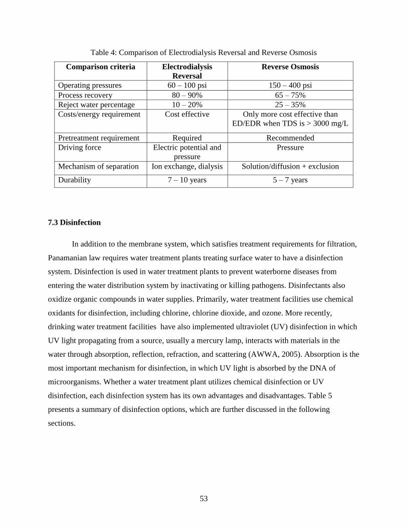
53

Table 4: Comparison of Electrodialysis Reversal and Reverse Osmosis

Comparison criteria Electrodialysis

Reversal

Reverse Osmosis

Operating pressures 60 – 100 psi 150 – 400 psi

Process recovery 80 – 90% 65 – 75%

Reject water percentage 10 – 20% 25 – 35%

Costs/energy requirement Cost effective Only more cost effective than

ED/EDR when TDS is > 3000 mg/L

Pretreatment requirement Required Recommended

Driving force Electric potential and

pressure

Pressure

Mechanism of separation Ion exchange, dialysis Solution/diffusion + exclusion

Durability 7 – 10 years 5 – 7 years

7.3 Disinfection

In addition to the membrane system, which satisfies treatment requirements for filtration,

Panamanian law requires water treatment plants treating surface water to have a disinfection

system. Disinfection is used in water treatment plants to prevent waterborne diseases from

entering the water distribution system by inactivating or killing pathogens. Disinfectants also

oxidize organic compounds in water supplies. Primarily, water treatment facilities use chemical

oxidants for disinfection, including chlorine, chlorine dioxide, and ozone. More recently,

drinking water treatment facilities have also implemented ultraviolet (UV) disinfection in which

UV light propagating from a source, usually a mercury lamp, interacts with materials in the

water through absorption, reflection, refraction, and scattering (AWWA, 2005). Absorption is the

most important mechanism for disinfection, in which UV light is absorbed by the DNA of

microorganisms. Whether a water treatment plant utilizes chemical disinfection or UV

disinfection, each disinfection system has its own advantages and disadvantages. Table 5

presents a summary of disinfection options, which are further discussed in the following

sections.

54

Table 5: Characteristics of Disinfectants (adapted from MWH, 2005)

Disinfectant

Characteristic Chlorine Chlorine

Dioxide

Ozone Ultraviolet

light

Inactivation of:

Bacteria

Excellent

Excellent

Excellent

Good

Viruses Excellent Excellent Excellent Fair

Protozoa Fair to poor Good Good Excellent

Endospores Good to poor Fair Excellent Fair

Frequency of use as

Primary Disinfectant

Most Common Occasional Common Emerging Use

Regulatory limit on

Residuals

4 mg/L 0.8 mg/L Not Applicable Not Applicable

Formation of

Regulated

Byproducts

4 THMs;

5 HAAs

Chlorite Bromate None

Formation of Other

Byproducts

Cyanogen

halides,

NDMA

Chlorate Biodegradable

organic carbon

None Known

Typical Dose, mg/L

(kg/ML)

1 – 6 0.2 – 1.5 1 – 5 20 – 100

mJ/cm2

Typical Dose, lb/MG 8 – 50 2 – 13 8 – 42 Not Applicable

7.3.1 Chlorine

Chlorine disinfection is widely used in the drinking water industry as a disinfectant.

Chlorine effectively inactivates a wide range of waterborne pathogens, produces a free chlorine

residual in the system that ensures the drinking water is properly disinfected, and has the lowest

relative costs to other disinfectant chemicals. In addition, chlorine serves as an oxidizing agent to

oxidize naturally occurring organic and inorganic compounds found in water. Chlorine

disinfection prevents algal growth in treatment systems, removes potential scale-forming metals

like iron and manganese, oxidizes hydrogen sulfide, and bleaches organic dyes which

compromise the aesthetics of the drinking water. However, chlorine produces disinfection by-

products when it reacts with organic matter. Some of these byproducts are known or suspected

carcinogens. Also, there is a health and safety concern when chlorine gas is administered into a

treatment system since the gas is classified by the U.S. Department of Transportation as

poisonous (HDR Engineering, Inc., 2001). Chlorine can be applied as a gas, liquid or solid.

Chlorine is delivered as liquid gas in tank cars, 1 ton and 150 lb cylinders, or as liquid bleach

55

which can be generated onsite from salt and water using electrolysis. In very small applications,

calcium hypochlorite powder is also used as a source for chlorine disinfection. In the past,

chlorine was added at the beginning of the plant and residual was carried through. Increasingly,

engineered contactors are used (MWH, 2005).

7.3.2 Chlorine Dioxide

Not as widely used as chlorine, another disinfectant used in drinking water treatment is

chlorine dioxide. This disinfectant is effective in destroying phenols and other organics in water

without the formation of the byproducts trihalomethanes (TTHs) and haloacetic acids (HAAs),

which are formed during chlorine disinfection. Chlorine dioxide does not dissociate or

disproportionate as chlorine does at normal drinking water pH levels (~ 6 to 10) and as a result is

a faster acting disinfectant than chlorine at higher pH levels. It exerts a demand when it is first

added to a water supply, which must be overcome if a persistent residual is to be maintained

throughout the system. Like chlorine, chlorine dioxide is photosensitive, and because it is a gas

at temperatures above 11°C, its residuals are easily removed by aeration. It is unsafe to store

chlorine dioxide once it is generated because it is a gas that readily reacts with multiple stimuli.

An increase in temperature, exposure to light, changes in pressure, and exposure to organic

contaminants in the water may cause the pure gas to explode. As a result, chlorine dioxide is

usually generated through a two-chemical oxidative process, in which chlorine, either as a gas or

in solution, is mixed with a 25 percent sodium chlorite (NaClO2) solution. It can also be

generated by direct electrolysis of sodium chlorite as powder or stabilized liquid solution. In the

past, chlorine dioxide was typically added at the beginning of the plant and residual was carried

through. Increasingly, engineered contactors are used. Chlorine dioxide has gained popularity

throughout Western Europe and the United States because the disinfectant does not form the

undesirable byproducts formed by chlorine disinfection. Still, there is concern that there are other

organic byproducts of chlorine dioxide that are not yet well understood, and it may have other

undesirable reaction products (AWWA, 2005).

7.3.3 Ozone

An allotrope of oxygen with three oxygen atoms, ozone (O3) is a strong oxidative gas. As

a result, extended exposure to ozone-containing air is harmful. At high concentrations (>23

56

percent) ozone is unstable (explosive) and under ambient conditions it undergoes rapid decay.

Therefore, unlike chlorine gas, it cannot be stored inside pressurized vessels and transported to

the water treatment plant (HDR Engineering, Inc., 2001). Consequently, like chlorine dioxide,

ozone must be generated onsite. Ozone is manufactured onsite using a corona discharge in dry

air or pure oxygen. Oxygen is usually delivered as a liquid. In some large plants, oxygen is also

manufactured onsite (MWH, 2005).

Once dissolved in water, ozone begins a process of decay that results in the formation of

the hydroxyl radical. For the inactivation of microorganisms and chemical breakdown of

organics in water, ozone reacts in two ways: (1) by direct oxidation and (2) through the action of

hydroxyl radicals (HO•) generated during its decomposition. Treatment plants using ozone

disinfection require two components: (1) a mass transfer device for dissolving the ozone into the

water and (2) a contact chamber in which the disinfection reaction takes place. In practice these

two components have been combined by the introduction of the ozone into the water in large,

deep basins using porous diffusers. When designing an ozonation system there are many

challenges that must be addressed including: determining a means for estimating mass transfer of

ozone into the water, having an understanding of the kinetics of ozone decay, having an

understanding of the disinfection kinetics, and determining a means for estimating dispersion in

the reactor. For a full-scale water treatment design addressing all of these issues with a variety of

approaches can be difficult. In addition, since ozone is sparingly soluble, the facilities that are

required to introduce it into water are usually expensive (HDR Engineering, Inc., 2001). Ozone

has always been added in specially engineered contactors. Currently, these contactors are using

more compartments and other techniques are being experimented with (MWH, 2005).

7.3.4 Ultraviolet Disinfection

Disinfection by ultraviolet (UV) radiation inactivates microorganisms by absorption of

light, which causes a photochemical reaction that alters molecular components essential to cell

function. UV radiation is excellent when disinfecting microorganisms such as bacteria and

viruses. Higher dosages of UV energy are required for the inactivation of protozoa such as

Giardia and Cryptosporidium. In addition, no undesired by-products or residual remain as a

result of UV disinfection; UV radiation [via electromagnetic waves] quickly dissipates into

water, to be absorbed or reflected off material within the water. For germicidal purposes the

57

optimal UV range is between 245 and 285 nm. Within a disinfection system low-pressure lamps

emit maximum energy output at a wavelength of 253.7 nm, and medium-pressure lamps emit

energy at wavelengths from 180 to 1370 nm. Lamps that emit at other wavelengths in a high-

intensity “pulsed” manner can also be utilized (HDR Engineering, Inc., 2001). Ultraviolet light

lamps are placed in gravity channels or in specially manufactured UV reactors. Because the

contact time is so short, reactors must be tested for short circuiting (MWH, 2005).

7.3.5 Disinfection Process Selection

Since the water treatment plant was designed for treating water in Panama, the team

considered the suitability of each disinfectant and its accompanying system to its application in

the country of Panama which is undergoing aggressive infrastructure development (CIA, 2012).

Although an excellent oxidative chemical, chlorine produces undesirable byproducts that would

require an additional removal process, increasing costs and complexity to the system by the

introduction of another system. Chlorine dioxide is suited for more sophisticated and equipped

facilities as it requires mixing tanks and chlorine dioxide is a highly reactive and dangerous gas.

Since ozone is sparingly soluble, an additional system is needed to facilitate the mass transfer of

ozone into water and a contact tank is needed for chemical reaction. In contrast, UV disinfection

is cost-effective and does not produce unwanted byproducts. In addition, UV lamps can be

installed with minimal maintenance or health concerns.

7.4 Water Treatment Plant Design

In the EDR process, polarity reversal is used to dissolve and flush precipitated salts from

the brine out of the system without involving any chemical pretreatment (HDR Engineering, Inc.,

2001). Still, some form of pretreatment is necessary. For this application, a 5-micron cartridge

filter was chosen as a means of pretreatment. Cartridge filters are typically used for point-of-use

systems and for pretreatment in advance of membrane treatment systems. These filters can be

made out of membrane, fabric, or string filter mediums, which are supported by a filter element

and placed in a pressure vessel. In the design of a water treatment plant for Gatun Lake, the team

has referred to the drinking water treatment plant (DWTP) built in Abrera (Barcelona), Spain.

This plant was designed by General Electric and was put into operation in April 2009 (Valero et

al., 2011).

58

The DWTP in Abrera has a total flow of 58 MGD. The plant uses cartridge filters for

pretreatment and electrodialisys reversal units for treatment. Details of the process design are

shown in Table 6. The plant has 18 cartridge filters followed by 9 EDR modules. These numbers

include both processes in operation and those off-line for cleaning and maintenance. The design

was scaled up to a design for a 150 MGD plant for Panama City. As shown in Table 6, the

Panama City plant is designed with 48 cartridge filters and 24 EDR modules.

Table 6: The Main Characteristics of Abrera and Panama City Water Treatment Plants

Process Abrera Plant

(58 MGD)

Panama City Plant

(150 MGD)

Number 18 48

Pore Size 5 µm 5 µm

Flow per cartridge 3.2 MGD 3.125 MGD

Number of off-line filters 4 8

Modules 9 24

Stacks per module 64 64

Stacks (total) 576 1536

Number of off-line EDR

stacks

1 module = 64

stacks

3 modules = 192

stacks

A total of 18 cartridge filters with a pore size of 5 µm are used during the pretreatment

for the water flow of 58 MGD (Valero el al., 2011). Scaling up to 150 MGD, a total of 48

cartridge filters with a pore size of 5 µm will be needed.

Electrodialisys reversal was chosen for the desalination of the brackish water. The DWTP

of Abrera uses 9 modules with 576 stacks in double stage (Valero el al., 2011). Scaling up to a

water demand of 150 MGD will require 1536 EDR stacks in double stage as well.

The disinfection system designed for the Panama water treatment plant is based off of the

Orange County water district’s ground water replenishment system located in California. While

the Orange County plant design is not focused on treating brackish water, it is still applicable

because the design has the capability to desalinate water and incorporates some of the same

design components as the plant for Panama: microfiltration, reverse osmosis, and ultraviolet

disinfection. The treatment plant has a capacity to treat 70 million gallons of water per day.

Trojan UV Phox equipment is used for the UV disinfection system. The design incorporated 9

ultraviolet trains with three stainless steel vessels installed in a vertical row as well as 39 low

pressure, high output UV lamps in each of the two chambers within in the vessels (Chalmers et

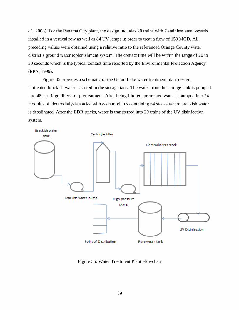
59

al., 2008). For the Panama City plant, the design includes 20 trains with 7 stainless steel vessels

installed in a vertical row as well as 84 UV lamps in order to treat a flow of 150 MGD. All

preceding values were obtained using a relative ratio to the referenced Orange County water

district’s ground water replenishment system. The contact time will be within the range of 20 to

30 seconds which is the typical contact time reported by the Environmental Protection Agency

(EPA, 1999).

Figure 35 provides a schematic of the Gatun Lake water treatment plant design.

Untreated brackish water is stored in the storage tank. The water from the storage tank is pumped

into 48 cartridge filters for pretreatment. After being filtered, pretreated water is pumped into 24

modulus of electrodialysis stacks, with each modulus containing 64 stacks where brackish water

is desalinated. After the EDR stacks, water is transferred into 20 trains of the UV disinfection

system.

Figure 35: Water Treatment Plant Flowchart

60

8.0 Conclusion

Current salinity levels in Gatun Lake were determined from water quality sampling

campaign conducted in 2011, which showed that the lake water is of freshwater quality. Then, a

modeling program was used to model salinity in the lake under current canal conditions

(Scenario 0) and future Post-Panamax conditions (Scenario 1). Modeling results showed that

salinity levels in Gatun Lake are expected to remain low after the expansion project is complete.

Namely, the results show that with the current lock system in operation the conditions of Gatun

Lake have remained consistent over time, up to the present-day. Furthermore, the results indicate

that salinity levels will remain consistent even with the operation of the Post-Panamax lock

system in the future. However, it is possible that the modeling efforts of Delft3D did not fully

capture the future water quality of Gatun Lake or that changes in canal operation could cause

future changes to the salinity in Gatun Lake. Based on these potential issues, a drinking water

treatment plant was designed to treat water from Gatun Lake assuming it was brackish. Based on

treatment process research and requirements in Panamanian for the treatment of surface waters,

the final design incorporated an EDR system for salt removal and UV light for disinfection.

61

9.0 References

Autoridad del Canal de Panamá. Anuario Hidrologico 2010; Republica de Panamá, April 2011.

[Online] http://www.pancanal.com/esp/cuenca/anuario-hidrologico/2010.pdf

Autoridad del Canal de Panamá. Informe de Calidad de Agua: De La Cuenca del Canal 2008-

2009; Metodología, 2; Panama. 2010. [Print]

All About Water. Reverse Osmosis, 2004 [Online] http://www.allaboutwater.org/reverse-

osmosis.html

American Public Health Association. Standard Methods for the Examination of Water and

Wastewater, 22; American Public Health Association, Washington, D.C., 2005.

American Water Works Association, American Society of Civil Engineers. Water Treatment

Plant Design, 4; Mc-Graw Hill, Inc., 2005.

Central Intelligence Agency. The World Fact Book: Panama, 2012 [Online]

https://www.cia.gov/library/publications/the-world-factbook/geos/pm.html

Chalmers B., Patel M., Dunivin B., Cutler D. Orange County Water District’s Groundwater

Replenishment System Is Now Producing Water, Water Environment Federation. 2008

[Online]

http://www.ingentaconnect.com/content/wef/wefproc/2008/00002008/00000012/art0002

3

Dean, R.G. and Dalrymple R.A. Water wave mechanics for engineers and scientists, Singapore:

World Scientific, 1991. [Print]

Delft Hydraulics. Delft3D-FLOW: Simulation of multi-dimensional hydrodynamic flows and

transport phenomena, including sediments, Deltares, Rotterdamseweg 185, September,

2010; Version 3.14. [Print]

62

DHI Water and Environment. Review of Saltwater Intrusion and Mitigation Studies and Models

for Proposed Post Panamax Locks, November 2005 [Online]

http://www.pancanal.com/esp/plan/estudios/0276-exec.pdf

E.S.P. Water Products. Reverse Osmosis Membrane, 2009 [Online]

http://espwaterproducts.com/about-reverse-osmosis.htm

Fernandez P. C. and Schattanek G. The Panama Canal: environmental aspects, sustainability

and global effects on greenhouse gases, November 2010 [Online]

http://www.citiesandports2010.com/pdf/orales_texte/ARG_TEXT_g-schattanek_p-

clemente.pdf

Greene, J. The Canal Builders: Making America's Empire at the Panama Canal, New York:

Penguin, 2009. [Print]

HDR Engineering, Inc. Handbook of Public Water Systems: Second Edition, Wiley. March 2011.

[Print]

Hubbard, K. Central America Cities: The Biggest Cities in Central America, Central America

Travel Guide. 2010 [Online]

http://gocentralamerica.about.com/od/tripplanning/a/Central-America-Cities.htm

Jongeling T., Hulsbergen R., and Schwanenberg D. Water Quality Model of Gatun Lake for

Expanded Panama Canal: Part I Modeling of the Present Situation, December 2008.

[Print]

Jongeling T., Zijl F., and Hulsbergen R. Water Quality Model of Gatun Lake for Expanded

Panama Canal: Part II Modeling of the Future Situation, March 2009. [Print]

Komar, P. Beach processes and sedimentation, Englewood Cliffs, NJ: Prentice-Hall, Inc., 1976.

[Print]

63

Louis Berger International, Inc. Development of Panama Canal Growth Strategy, The Port

Authority of New York & New Jersey. [Online]

http://www.pancanal.com/esp/plan/estudios/ep-0010-03.pdf

Martin C. What is the nutrient cycle? WiseGEEK, 2011. [Online]

http://www.wisegeek.com/what-is-the-nutrient-cycle.htm

Martinez K. Panama to vote on Canal Expansion Oct. 22, Washington Post, 2006. [Online]

http://www.washingtonpost.com/wp-

dyn/content/article/2006/07/16/AR2006071600470.html

McCullough, D. G. The Path between the Seas: the Creation of the Panama Canal, 1870-1914.

New York: Simon and Schuster, 1977. [Print]

Montgomery Watson Harza. Water Treatment: Principles and Design, 2; John Wiley & Sons,

Inc: Hoboken, New Jersey, 2005. [Print]

Nature Grid. Algae, 2011 [Online]

http://www.naturegrid.org.uk/biodiversity/plants/crypalga.html#feed

Office of Naval Research. Ocean Water: Salinity, 2011 [Online]

http://www.onr.navy.mil/focus/ocean/water/salinity1.htm

Panama Canal Authority. ACP Overview, 2011a [Online]

http://www.pancanal.com/eng/general/acp-overview.html

Panama Canal Authority. Category III Environmental Impact Study, Panama Canal Expansion

Project – Third Set of Locks, July 2007 [Online]

http://www.pancanal.com/eng/expansion/eisa/chap-04.pdf

64

Panama Canal Authority. Proposal for the Expansion of the Panama Canal, 24 April, 2006b.

[Online] http://www.acp.gob.pa/eng/plan/documentos/propuesta/acp-expansion-

proposal.pdf

Panama Canal Authority. Third Set of Locks Project, 24 April, 2006a. [Online]

http://www.pancanal.com/esp/plan/documentos/propuesta/acp-proposla-relevant-

information.pdf

Panama Canal Authority. This is the Canal, 2011b [Online]

http://www.pancanal.com/eng/acp/asi-es-el-canal.html

Panama Canal Authority. Trade Routes, 2011c [Online]

http://www.pancanal.com/eng/maritime/routes.html

Panama Canal Authority. Vessel Requirements, 2005 [Online]

http://www.pancanal.com/eng/maritime/notices/n01-05.pdf

Parchure T. M., Wilhelms S. C., Sarruff S., and McAnally W. H. Salinity Intrusion in the

Panama Canal, April 2000, [Online] http://www.dtic.mil/cgi-

bin/GetTRDoc?Location=U2&doc=GetTRDoc.pdf&AD=ADA378475

Sea-Bird Electronics, Inc. SBE 19plus SEACAT Profiler User’s Manual, December 2007

[Online] http://www.seabird.com/pdf_documents/manuals/19plus_017.pdf

Simon, F.X., Penru Y., Guastalli A.R., Llorens J., and Baig S. Improvement of the Analysis of the

Biochemical Oxygen Demand (BOD) of Mediterranean Seawater by Seeding Control,

Atlanta, 85.1 (2011): 527-32.

Stubbs H.S., Spence L., Hall C., and Ostendorff M. Algae for better or worse, Science

Activities: Classroom projects and curriculum ideas, 3 April 2010 [Online]

http://www.tandfonline.com/doi/pdf/10.1080/00368120209601070

65

Thatcher T.L. and Layton D.W. Deposition, resuspension, and penetration of particles within a

residence, Atmospheric Environment, Vol.29, No. 13, 1995, Elsevier Science Ltd.

The National Center for Supercomputing Applications. Density Currents, 2006 [Online]

http://access.ncsa.illinois.edu/Stories/DensityCurrents/

Trussel Technologies. Desalination Technologies, Pasadena. 2008. [Online]

http://www.trusselltech.com/tech_desalination.asp

TSC’s Water Treatment Engineering Team. Electrodialysis (ED) and Electrodialysis Reversal

(EDR), U.S. Department of the Interior, September 2010. [Online]

http://www.usbr.gov/pmts/water/publications/reportpdfs/Primer%20Files/07%20-

%20Electrodialysis.pdf

Uhrikova D. Adsorption, 2011. [Online]

http://www.fpharm.uniba.sk/fileadmin/user_upload/english/Physical_Chemistry/5-

Adsorption.pdf

United States Environmental Protection Agency. Wastewater Technology Fact Sheet: Ultraviolet

Disinfection, Municipal Technology Branch U.S. EPA, 1999. [Online]

http://water.epa.gov/scitech/wastetech/upload/2002_06_28_mtb_uv.pdf

University of Wisconsin School of Freshwater Sciences. The Niskin Bottle, November 2011

[Online] http://www.glwi.uwm.edu/education/outreach/cruise/niskin.php

URS Holdings, Inc. Tropical Lake Ecology Assessment with Emphasis on Changes in Salinity of

Lakes, December 2004 [Online] http://www.pancanal.com/esp/plan/estudios/0261-03.pdf

Valero F., Barcelo A. & Arbos R. Electrodialysis Technology, Theory and Application.

Desalination, Trends and Technologies. [Online]

http://www.intechopen.com/source/pdfs/13751/InTech_Electrodialysis_technology_theor

y_and_applications.pdf

66

Webb D. Water quality variations during nitrification in drinking water distribution systems,

University of Central Florida, 2004. [Online]

http://etd.fcla.edu/CF/CFE0000063/Webb_David_W_200405_MSEnvE.pdf