Salient Object Detection via Bootstrap Learning Na Tong 1 , Huchuan Lu 1 , Xiang Ruan 2 and Ming-Hsuan Yang 3 1 Dalian University of Technology 2 OMRON Corporation 3 University of California at Merced Abstract We propose a bootstrap learning algorithm for salient object detection in which both weak and strong models are exploited. First, a weak saliency map is constructed based on image priors to generate training samples for a strong model. Second, a strong classifier based on samples direct- ly from an input image is learned to detect salient pixels. Results from multiscale saliency maps are integrated to fur- ther improve the detection performance. Extensive experi- ments on six benchmark datasets demonstrate that the pro- posed bootstrap learning algorithm performs favorably a- gainst the state-of-the-art saliency detection methods. Fur- thermore, we show that the proposed bootstrap learning ap- proach can be easily applied to other bottom-up saliency models for significant improvement. 1. Introduction As an important preprocessing step in computer vision problems to reduce computational complexity, saliency de- tection has attracted much attention in recent years. Al- though significant progress has been made, it remains a challenging task to develop effective and efficient algo- rithms for salient object detection. Saliency models include two main research areas: vi- sual attention which is extensively studied in neuroscience and cognitive modeling, and salient object detection which is of great interest in computer vision. Salient object de- tection methods can be categorized as bottom-up stimuli- driven [1, 8–12, 15–18, 20, 23, 28–38, 41, 43] and top-down task-driven [19, 40, 42] approaches. Bottom-up methods are usually based on low-level visual information and are more effective in detecting fine details rather than global shape information. In contrast, top-down saliency model- s are able to detect objects of certain sizes and categories based on more representative features from training sam- ples. However, the detection results from top-down meth- ods tend to be coarse with fewer details. In terms of com- putational complexity, bottom-up methods are often more efficient than top-down approaches. In this paper, we propose a novel algorithm for salien- Figure 1. Saliency maps generated by the proposed method. Brighter pixels indicate higher saliency values. Left to right: in- put, ground truth, weak saliency map, strong saliency map, and final saliency map. t object detection via bootstrap learning [22]. To address the problems of noisy detection results and limited repre- sentations from bottom-up methods, we present a learning approach to exploit multiple features. However, unlike ex- isting top-down learning-based methods, the proposed algo- rithm is bootstrapped with samples from a bottom-up mod- el, thereby alleviating the time-consuming off-line training process or labeling positive samples manually. 2. Related Work and Problem Context Both weak and strong learning models are exploited in the proposed bootstrap learning algorithm. First, we com- pute a weak contrast-based saliency map based on super- pixels of an input image. This coarse saliency map is s- moothed by a graph cut method, where a set of training samples is collected, where positive samples are pertaining to the salient objects while negative samples are from the background in this image. Next, a strong classifier based on Multiple Kernel Boosting (MKB) [39] is learned to measure saliency where three feature descriptors (RGB, CIELab col- or pixels, and the Local Binary Pattern histograms) are ex- tracted and four kernels (linear, polynomial, RBF, and sig- moid functions) are used to exploit rich feature representa- tions. Furthermore, we use multiscale superpixels to detect salient objects of varying sizes. As the weak saliency mod- el tends to detect fine details and the strong saliency model focuses on global shapes, these two are combined to gener- ate the final saliency map. Experiments on six benchmark

Welcome message from author
This document is posted to help you gain knowledge. Please leave a comment to let me know what you think about it! Share it to your friends and learn new things together.
Transcript
Salient Object Detection via Bootstrap Learning
Na Tong1, Huchuan Lu1, Xiang Ruan2 and Ming-Hsuan Yang3
1Dalian University of Technology 2OMRON Corporation 3University of California at Merced
Abstract
We propose a bootstrap learning algorithm for salient
object detection in which both weak and strong models are
exploited. First, a weak saliency map is constructed based
on image priors to generate training samples for a strong
model. Second, a strong classifier based on samples direct-
ly from an input image is learned to detect salient pixels.
Results from multiscale saliency maps are integrated to fur-
ther improve the detection performance. Extensive experi-
ments on six benchmark datasets demonstrate that the pro-
posed bootstrap learning algorithm performs favorably a-
gainst the state-of-the-art saliency detection methods. Fur-
thermore, we show that the proposed bootstrap learning ap-
proach can be easily applied to other bottom-up saliency
models for significant improvement.
1. Introduction
As an important preprocessing step in computer vision
problems to reduce computational complexity, saliency de-
tection has attracted much attention in recent years. Al-
though significant progress has been made, it remains a
challenging task to develop effective and efficient algo-
rithms for salient object detection.
Saliency models include two main research areas: vi-
sual attention which is extensively studied in neuroscience
and cognitive modeling, and salient object detection which
is of great interest in computer vision. Salient object de-
tection methods can be categorized as bottom-up stimuli-
driven [1, 8–12, 15–18, 20, 23, 28–38, 41, 43] and top-down
task-driven [19, 40, 42] approaches. Bottom-up methods
are usually based on low-level visual information and are
more effective in detecting fine details rather than global
shape information. In contrast, top-down saliency model-
s are able to detect objects of certain sizes and categories
based on more representative features from training sam-
ples. However, the detection results from top-down meth-
ods tend to be coarse with fewer details. In terms of com-
putational complexity, bottom-up methods are often more
efficient than top-down approaches.
In this paper, we propose a novel algorithm for salien-
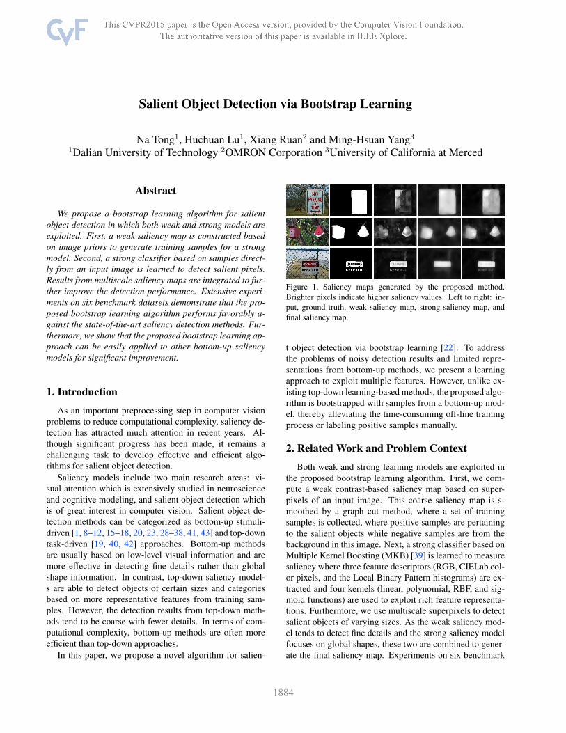
Figure 1. Saliency maps generated by the proposed method.
Brighter pixels indicate higher saliency values. Left to right: in-
put, ground truth, weak saliency map, strong saliency map, and
final saliency map.
t object detection via bootstrap learning [22]. To address
the problems of noisy detection results and limited repre-
sentations from bottom-up methods, we present a learning
approach to exploit multiple features. However, unlike ex-
isting top-down learning-based methods, the proposed algo-
rithm is bootstrapped with samples from a bottom-up mod-
el, thereby alleviating the time-consuming off-line training
process or labeling positive samples manually.
2. Related Work and Problem Context
Both weak and strong learning models are exploited in
the proposed bootstrap learning algorithm. First, we com-
pute a weak contrast-based saliency map based on super-
pixels of an input image. This coarse saliency map is s-
moothed by a graph cut method, where a set of training
samples is collected, where positive samples are pertaining
to the salient objects while negative samples are from the
background in this image. Next, a strong classifier based on
Multiple Kernel Boosting (MKB) [39] is learned to measure
saliency where three feature descriptors (RGB, CIELab col-
or pixels, and the Local Binary Pattern histograms) are ex-
tracted and four kernels (linear, polynomial, RBF, and sig-
moid functions) are used to exploit rich feature representa-
tions. Furthermore, we use multiscale superpixels to detect
salient objects of varying sizes. As the weak saliency mod-
el tends to detect fine details and the strong saliency model
focuses on global shapes, these two are combined to gener-
ate the final saliency map. Experiments on six benchmark
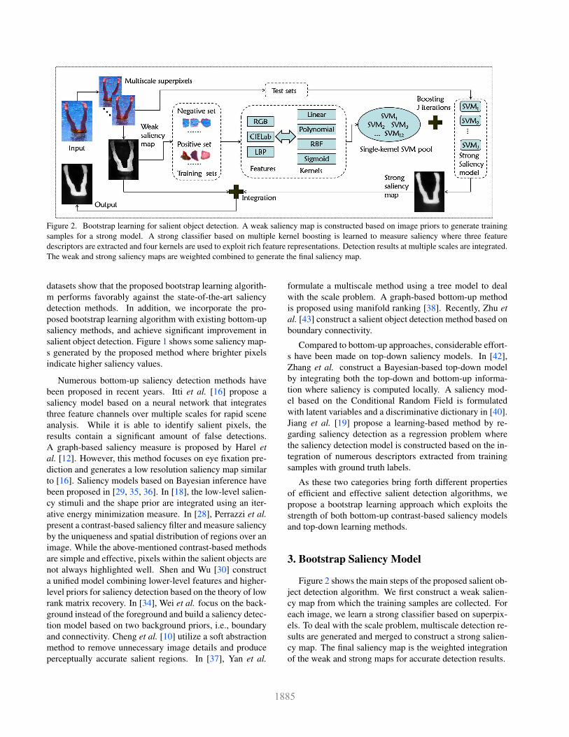
Figure 2. Bootstrap learning for salient object detection. A weak saliency map is constructed based on image priors to generate training
samples for a strong model. A strong classifier based on multiple kernel boosting is learned to measure saliency where three feature
descriptors are extracted and four kernels are used to exploit rich feature representations. Detection results at multiple scales are integrated.
The weak and strong saliency maps are weighted combined to generate the final saliency map.
datasets show that the proposed bootstrap learning algorith-
m performs favorably against the state-of-the-art saliency
detection methods. In addition, we incorporate the pro-
posed bootstrap learning algorithm with existing bottom-up
saliency methods, and achieve significant improvement in
salient object detection. Figure 1 shows some saliency map-
s generated by the proposed method where brighter pixels
indicate higher saliency values.
Numerous bottom-up saliency detection methods have
been proposed in recent years. Itti et al. [16] propose a
saliency model based on a neural network that integrates
three feature channels over multiple scales for rapid scene
analysis. While it is able to identify salient pixels, the
results contain a significant amount of false detections.
A graph-based saliency measure is proposed by Harel et
al. [12]. However, this method focuses on eye fixation pre-
diction and generates a low resolution saliency map similar
to [16]. Saliency models based on Bayesian inference have
been proposed in [29, 35, 36]. In [18], the low-level salien-
cy stimuli and the shape prior are integrated using an iter-
ative energy minimization measure. In [28], Perrazzi et al.
present a contrast-based saliency filter and measure saliency
by the uniqueness and spatial distribution of regions over an
image. While the above-mentioned contrast-based methods
are simple and effective, pixels within the salient objects are
not always highlighted well. Shen and Wu [30] construct
a unified model combining lower-level features and higher-
level priors for saliency detection based on the theory of low
rank matrix recovery. In [34], Wei et al. focus on the back-
ground instead of the foreground and build a saliency detec-
tion model based on two background priors, i.e., boundary
and connectivity. Cheng et al. [10] utilize a soft abstraction
method to remove unnecessary image details and produce
perceptually accurate salient regions. In [37], Yan et al.
formulate a multiscale method using a tree model to deal
with the scale problem. A graph-based bottom-up method
is proposed using manifold ranking [38]. Recently, Zhu et
al. [43] construct a salient object detection method based on
boundary connectivity.
Compared to bottom-up approaches, considerable effort-
s have been made on top-down saliency models. In [42],
Zhang et al. construct a Bayesian-based top-down model
by integrating both the top-down and bottom-up informa-
tion where saliency is computed locally. A saliency mod-
el based on the Conditional Random Field is formulated
with latent variables and a discriminative dictionary in [40].
Jiang et al. [19] propose a learning-based method by re-
garding saliency detection as a regression problem where
the saliency detection model is constructed based on the in-
tegration of numerous descriptors extracted from training
samples with ground truth labels.
As these two categories bring forth different properties
of efficient and effective salient detection algorithms, we
propose a bootstrap learning approach which exploits the
strength of both bottom-up contrast-based saliency models
and top-down learning methods.
3. Bootstrap Saliency Model
Figure 2 shows the main steps of the proposed salient ob-
ject detection algorithm. We first construct a weak salien-
cy map from which the training samples are collected. For
each image, we learn a strong classifier based on superpix-
els. To deal with the scale problem, multiscale detection re-
sults are generated and merged to construct a strong salien-
cy map. The final saliency map is the weighted integration
of the weak and strong maps for accurate detection results.
3.1. Image Features
Superpixels have been used extensively in vision tasks
as the basic units to capture the local structural information.
In this paper, we compute a fixed number of superpixels
from an input image using the Simple Linear Iterative Clus-
tering (SLIC) method [2]. Three descriptors including the
RGB, CIELab and Local Binary Pattern (LBP) features are
used to describe each superpixel. The rationale to use two
different color representations is based on empirical results
where better detection performance is achieved when both
are used, which can be found in the supplementary docu-
ment. We consider the LBP features in a 3 × 3 neighbor-
hood of each pixel. Next, each pixel is assigned to a value
between 0 and 58 in the uniform pattern [27]. We construct
an LBP histogram for each superpixel, i.e., a vector of 59dimensions ({hi}, i = 1, 2, ...59, where hi is the value of
the i-th bin in an LBP histogram).
3.2. Weak Saliency Model
The center-bias prior has been shown to be effective in
salient object detection [5, 25]. Based on this assumption,
we develop a method to construct a weak saliency model by
exploiting the contrast between each region and the region-
s along the image border. However, existing contrast-based
methods usually generate noisy results since low-level visu-
al cues are limited. In this paper, we exploit the center-bias
and dark channel priors to better estimate saliency maps.
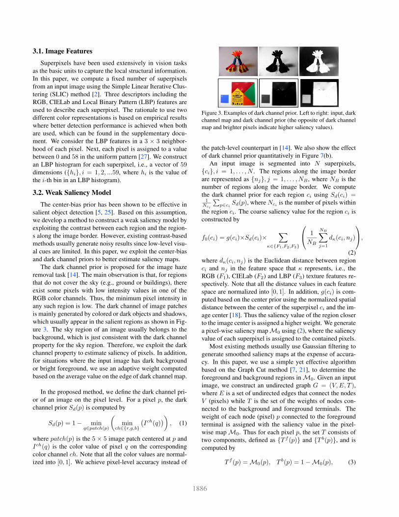
The dark channel prior is proposed for the image haze
removal task [14]. The main observation is that, for regions
that do not cover the sky (e.g., ground or buildings), there
exist some pixels with low intensity values in one of the
RGB color channels. Thus, the minimum pixel intensity in
any such region is low. The dark channel of image patches
is mainly generated by colored or dark objects and shadows,
which usually appear in the salient regions as shown in Fig-
ure 3. The sky region of an image usually belongs to the
background, which is just consistent with the dark channel
property for the sky region. Therefore, we exploit the dark
channel property to estimate saliency of pixels. In addition,
for situations where the input image has dark background
or bright foreground, we use an adaptive weight computed
based on the average value on the edge of dark channel map.
In the proposed method, we define the dark channel pri-
or of an image on the pixel level. For a pixel p, the dark
channel prior Sd(p) is computed by
Sd(p) = 1− minq∈patch(p)
(
minch∈{r,g,b}
(
Ich(q))
)
, (1)
where patch(p) is the 5 × 5 image patch centered at p and
Ich(q) is the color value of pixel q on the corresponding
color channel ch. Note that all the color values are normal-
ized into [0, 1]. We achieve pixel-level accuracy instead of
Figure 3. Examples of dark channel prior. Left to right: input, dark
channel map and dark channel prior (the opposite of dark channel
map and brighter pixels indicate higher saliency values).
the patch-level counterpart in [14]. We also show the effect
of dark channel prior quantitatively in Figure 7(b).
An input image is segmented into N superpixels,
{ci}, i = 1, . . . , N . The regions along the image border
are represented as {nj}, j = 1, . . . , NB , where NB is the
number of regions along the image border. We compute
the dark channel prior for each region ci using Sd(ci) =1
Nci
∑
p∈ciSd(p), where Nci is the number of pixels within
the region ci. The coarse saliency value for the region ci is
constructed by
f0(ci) = g(ci)×Sd(ci)×∑
κ∈{F1,F2,F3}
1
NB
NB∑
j=1
dκ(ci, nj)
,
(2)
where dκ(ci, nj) is the Euclidean distance between region
ci and nj in the feature space that κ represents, i.e., the
RGB (F1), CIELab (F2) and LBP (F3) texture features re-
spectively. Note that all the distance values in each feature
space are normalized into [0, 1]. In addition, g(ci) is com-
puted based on the center prior using the normalized spatial
distance between the center of the superpixel ci and the im-
age center [18]. Thus the saliency value of the region closer
to the image center is assigned a higher weight. We generate
a pixel-wise saliency map M0 using (2), where the saliency
value of each superpixel is assigned to the contained pixels.
Most existing methods usually use Gaussian filtering to
generate smoothed saliency maps at the expense of accura-
cy. In this paper, we use a simple yet effective algorithm
based on the Graph Cut method [7, 21], to determine the
foreground and background regions in M0. Given an input
image, we construct an undirected graph G = (V,E, T ),where E is a set of undirected edges that connect the nodes
V (pixels) while T is the set of the weights of nodes con-
nected to the background and foreground terminals. The
weight of each node (pixel) p connected to the foreground
terminal is assigned with the saliency value in the pixel-
wise map M0. Thus for each pixel p, the set T consists of
two components, defined as {T f (p)} and {T b(p)}, and is
computed by
T f (p) = M0(p), T b(p) = 1−M0(p), (3)
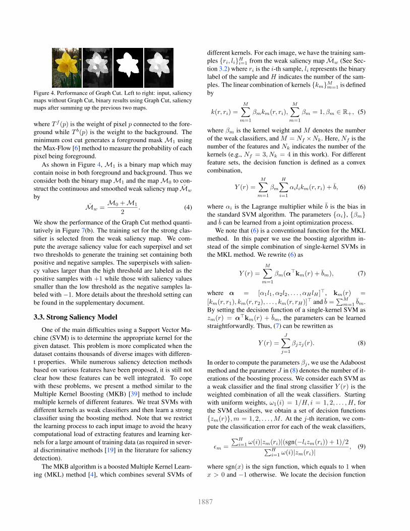
Figure 4. Performance of Graph Cut. Left to right: input, saliency
maps without Graph Cut, binary results using Graph Cut, saliency
maps after summing up the previous two maps.
where T f (p) is the weight of pixel p connected to the fore-
ground while T b(p) is the weight to the background. The
minimum cost cut generates a foreground mask M1 using
the Max-Flow [6] method to measure the probability of each
pixel being foreground.
As shown in Figure 4, M1 is a binary map which may
contain noise in both foreground and background. Thus we
consider both the binary map M1 and the map M0 to con-
struct the continuous and smoothed weak saliency map Mw
by
Mw =M0 +M1
2. (4)
We show the performance of the Graph Cut method quanti-
tatively in Figure 7(b). The training set for the strong clas-
sifier is selected from the weak saliency map. We com-
pute the average saliency value for each superpixel and set
two thresholds to generate the training set containing both
positive and negative samples. The superpixels with salien-
cy values larger than the high threshold are labeled as the
positive samples with +1 while those with saliency values
smaller than the low threshold as the negative samples la-
beled with −1. More details about the threshold setting can
be found in the supplementary document.
3.3. Strong Saliency Model
One of the main difficulties using a Support Vector Ma-
chine (SVM) is to determine the appropriate kernel for the
given dataset. This problem is more complicated when the
dataset contains thousands of diverse images with differen-
t properties. While numerous saliency detection methods
based on various features have been proposed, it is still not
clear how these features can be well integrated. To cope
with these problems, we present a method similar to the
Multiple Kernel Boosting (MKB) [39] method to include
multiple kernels of different features. We treat SVMs with
different kernels as weak classifiers and then learn a strong
classifier using the boosting method. Note that we restrict
the learning process to each input image to avoid the heavy
computational load of extracting features and learning ker-
nels for a large amount of training data (as required in sever-
al discriminative methods [19] in the literature for saliency
detection).
The MKB algorithm is a boosted Multiple Kernel Learn-
ing (MKL) method [4], which combines several SVMs of
different kernels. For each image, we have the training sam-
ples {ri, li}Hi=1 from the weak saliency map Mw (See Sec-
tion 3.2) where ri is the i-th sample, li represents the binary
label of the sample and H indicates the number of the sam-
ples. The linear combination of kernels {km}Mm=1 is defined
by
k(r, ri) =
M∑
m=1
βmkm(r, ri),
M∑
m=1
βm = 1, βm ∈ R+, (5)
where βm is the kernel weight and M denotes the number
of the weak classifiers, and M = Nf ×Nk. Here, Nf is the
number of the features and Nk indicates the number of the
kernels (e.g., Nf = 3, Nk = 4 in this work). For different
feature sets, the decision function is defined as a convex
combination,
Y (r) =
M∑
m=1
βm
H∑
i=1
αilikm(r, ri) + b, (6)
where αi is the Lagrange multiplier while b is the bias in
the standard SVM algorithm. The parameters {αi}, {βm}and b can be learned from a joint optimization process.
We note that (6) is a conventional function for the MKL
method. In this paper we use the boosting algorithm in-
stead of the simple combination of single-kernel SVMs in
the MKL method. We rewrite (6) as
Y (r) =
M∑
m=1
βm(α⊤km(r) + bm), (7)
where α = [α1l1, α2l2, . . . , αH lH ]⊤, km(r) =
[km(r, r1), km(r, r2), . . . , km(r, rH)]⊤ and b =∑M
m=1 bm.
By setting the decision function of a single-kernel SVM as
zm(r) = α⊤km(r) + bm, the parameters can be learned
straightforwardly. Thus, (7) can be rewritten as
Y (r) =J∑
j=1
βjzj(r). (8)
In order to compute the parameters βj , we use the Adaboost
method and the parameter J in (8) denotes the number of it-
erations of the boosting process. We consider each SVM as
a weak classifier and the final strong classifier Y (r) is the
weighted combination of all the weak classifiers. Starting
with uniform weights, ω1(i) = 1/H, i = 1, 2, . . . , H , for
the SVM classifiers, we obtain a set of decision functions
{zm(r)},m = 1, 2, . . . ,M . At the j-th iteration, we com-
pute the classification error for each of the weak classifiers,
ǫm =
∑Hi=1 ω(i)|zm(ri)|(sgn(−lizm(ri)) + 1)/2
∑Hi=1 ω(i)|zm(ri)|
, (9)
where sgn(x) is the sign function, which equals to 1 when
x > 0 and −1 otherwise. We locate the decision function
zj(r) with the minimum error ǫj , i.e., ǫj = min1≤m≤M ǫm.
Then the combination coefficient βj is computed by βj =12 log
1−ǫjǫj
· 12 (sgn(log
1−ǫjǫj
) + 1). Note that βj must be
larger than 0, indicating ǫj < 0.5, which accords with the
basic hypothesis that the boosting method could make the
weak classifiers into a strong one. In addition, we update
the weight using the following equation,
ωj+1(i) =ωj(i)e
−βj lizj(ri)
2√
ǫj(ǫj − 1). (10)
After J iterations, all the βj and zj(r) are computed and we
have a boosted classifier (8) as the saliency model learned
directly from an input image. We apply this strong salien-
cy model to the test samples (based on all the superpixels
of an input image), and a pixel-wise saliency map is thus
generated.
To improve the accuracy of the map, we first use the
Graph Cut method to smooth the saliency detection result-
s. Next, we obtain the strong saliency map Ms by further
enhancing the saliency map with the guided filter [13] as
it has been shown to perform well as an edge-preserving
smoothing operator.
3.4. Multiscale Saliency Maps
The accuracy of the saliency map is sensitive to the num-
ber of superpixels as salient objects are likely to appear at
different scales. To deal with the scale problem, we gen-
erate four layers of superpixels with different granularities,
where N = 100, 150, 200, 250 respectively. We represen-
t the weak saliency map (See Section 3.2) at each scale as
{Mwi} and the multiscale weak saliency map is comput-
ed by Mw = 14
∑4i=1 Mwi
. Next, the training sets from
the four scales are used to train one strong saliency model
and the test sets (based on all the superpixels from four s-
cales) are tested by the learned model simultaneously. Four
strong saliency maps from four scales are constructed (See
Section 3.3), denoted as {Msi}, i = 1, 2, 3, 4. Finally, we
obtain the final strong saliency map as Ms =14
∑4i=1 Msi .
As such, the proposed method is robust to scale variation.
3.5. Integration
The proposed weak and strong saliency maps have com-
plementary properties. The weak map is likely to detect fine
details and to capture local structural information due to the
contrast-based measure. In contrast, the strong map works
well by focusing on global shapes for most images except
the case when the test background samples have similari-
ty with the positive training set or large differences com-
pared to the negative training set, or vice versa for the test
foreground sample. In this case, the strong map may mis-
classify the test regions as shown in the bottom row of Fig-
ure 1. Thus we integrate these two maps by a weighted
combination,
M = σMs + (1− σ)Mw, (11)
where σ is a balance factor for the combination, and σ =0.7 to weigh the strong map more than the weak map, and
M is the final saliency map via bootstrap learning. More
discussions about the values of σ can be found in the sup-
plementary document.
4. Experimental Results
We present experimental results of 22 saliency detection
methods including the proposed algorithms on six bench-
mark datasets. The ASD dataset, selected from a bigger
image database [25], contains 1,000 images, and is labeled
with pixel-wise ground truth [1]. The THUS dataset [9]
consists of 10, 000 images where all images are labeled
with pixel-wise ground truth. The SOD dataset [26] is
composed of 300 images from the Berkeley segmentation
dataset where each one is labeled with salient object bound-
aries, based on which the pixel level ground truth [34] is
built. Some of the images in the SOD dataset include more
than one salient object. The SED2 dataset [3] contains 100images which are labeled with pixel-wise ground truth an-
notations. It is challenging due to the fact that every image
has two salient objects. The Pascal-S dataset [24] contains
850 images which are also labeled with pixel-wise ground
truth. For comprehensive evaluation, we use all the im-
ages in the Pascal-S dataset for test instead of using 40%for training and the rest for test as [24]. The DUT-OMRON
dataset [38] contains 5168 challenging images with pixel-
wise ground truth annotations. All the experiments are car-
ried out using MATLAB on a desktop computer with an In-
tel i7-3770 CPU (3.4 GHz) and 32GB RAM. For fair com-
parison, we use the original source code or the provided
saliency detection results in the literature. The MATLAB
source code is available on our project site.
We first evaluate the proposed algorithms and other 19
state-of-the-art methods including the IT98 [16], SF [28], L-
RMR [30], wCO [43], GS SP [34], XL13 [36], RA10 [29],
GB [12], LC [41], SR [15], FT [1], CA [11], SVO [8],
CBsal [18], GMR [38], GC [10], HS [37], RC-J [9] and
DSR [23] methods on the ASD, SOD, SED2, THUS and
DUT-OMRON datasets. In addition, the DRFI [19] method
uses images and ground truth for training, which contains
part of the ASD, THUS and SOD datasets, and the result-
s on the Pascal-S dataset are not provided. Accordingly,
we only compare our method with the DRFI model on the
SED2 dataset. Therefore, our methods are evaluated with
20 methods on the SED2 datasets. The MSRA [25] dataset
consists of 5,000 images. Since more than 3,700 images
in the MSRA dataset are included in the THUS dataset, we
do not present the evaluation results on this dataset due to
space limitations.
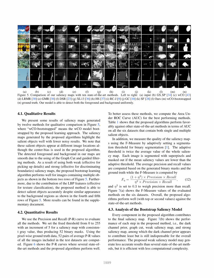
(a) (b) (c) (d) (e) (f) (g) (h) (i) (j) (k) (l) (m) (n)Figure 5. Comparison of our saliency maps with ten state-of-the-art methods. Left to right: (a) input (b) GS SP [34] (c) wCO [43]
(d) LRMR [30] (e) GMR [38] (f) DSR [23] (g) XL13 [36] (h) HS [37] (i) RC-J [9] (j) GC [10] (k) SF [28] (l) Ours (m) wCO-bootstrapped
(n) ground truth. Our model is able to detect both the foreground and background uniformly.
4.1. Qualitative Results
We present some results of saliency maps generated
by twelve methods for qualitative comparison in Figure 5,
where “wCO-bootstrapped” means the wCO model boot-
strapped by the proposed learning approach. The saliency
maps generated by the proposed algorithms highlight the
salient objects well with fewer noisy results. We note that
these salient objects appear at different image locations al-
though the center-bias is used in the proposed algorithm.
The detected foreground and background in our maps are
smooth due to the using of the Graph Cut and guided filter-
ing methods. As a result of using both weak (effective for
picking up details) and strong (effective for discriminating
boundaries) saliency maps, the proposed bootstrap learning
algorithm performs well for images containing multiple ob-
jects as shown in the bottom two rows of Figure 5. Further-
more, due to the contribution of the LBP features (effective
for texture classification), the proposed method is able to
detect salient objects accurately despite similar appearance
to the background regions as shown in the fourth and fifth
rows of Figure 5. More results can be found in the supple-
mentary document.
4.2. Quantitative Results
We use the Precision and Recall (P-R) curve to evaluate
all the methods. We set the fixed threshold from 0 to 255
with an increment of 5 for a saliency map with consisten-
t gray value, thus producing 52 binary masks. Using the
pixel-wise ground truth data, 52 pairs of average P-R values
of all the images included in the test datasets are comput-
ed. Figure 6 shows the P-R curves where several state-of-
the-art methods and the proposed algorithms perform well.
To better assess these methods, we compute the Area Un-
der ROC Curve (AUC) for the best performing methods.
Table 1 shows that the proposed algorithms perform favor-
ably against other state-of-the-art methods in terms of AUC
on all the six datasets that contain both single and multiple
salient objects.
In addition, we measure the quality of the saliency map-
s using the F-Measure by adaptively setting a segmenta-
tion threshold for binary segmentation [1]. The adaptive
threshold is twice the average value of the whole salien-
cy map. Each image is segmented with superpixels and
masked out if the mean saliency values are lower than the
adaptive threshold. The average precision and recall values
are computed based on the generated binary masks and the
ground truth while the F-Measure is computed by
Fη =(1 + η2)× Precision×Recall
η2 × Precision+Recall, (12)
and η2 is set to 0.3 to weigh precision more than recall.
Figure 7(a) shows the F-Measure values of the evaluated
methods on the six datasets. Overall, the proposed algo-
rithms perform well (with top or second values) against the
state-of-the-art methods.
4.3. Analysis of the Bootstrap Saliency Model
Every component in the proposed algorithm contributes
to the final saliency map. Figure 7(b) shows the perfor-
mance of each step in the proposed method, i.e., the dark
channel prior, graph cut, weak saliency map, and strong
saliency map, among which the dark channel prior appears
to contribute least but is still indispensable for the overall
performance. The proposed weak saliency model may gen-
erate less accurate results than several state-of-the-art meth-
ods, but it is efficient with less computational complexity.

HS 1 0.956859 0.932825 0.915226 0.901242 0.889679 0.879479
0.198502 0.529796 0.636434 0.689749 0.7209 0.74431 0.764197
Cbsal 1 0.971362 0.958368 0.947988 0.939012 0.930239 0.922293
0.198502 0.596668 0.689279 0.745228 0.784004 0.811859 0.833464
wCO 1 0.991373 0.984814 0.978828 0.972422 0.966175 0.959811
0.198502 0.34036 0.420089 0.487547 0.546427 0.598013 0.640131
GMR 1 0.996639 0.993223 0.988612 0.983668 0.978369 0.972685
0.198502 0.275404 0.340007 0.39482 0.444039 0.493797 0.542221
SF 1 0.96539 0.92304 0.881957 0.841839 0.801431 0.761542
0.198502 0.264398 0.34321 0.411997 0.473571 0.522639 0.565179
XL13 1 0.999299 0.996734 0.992776 0.98805 0.981953 0.974305
0.198502 0.236202 0.272545 0.302544 0.328963 0.353891 0.377825
GC 1 0.886054 0.843728 0.813928 0.790586 0.767664 0.747103
0.198502 0.705022 0.769759 0.803371 0.825166 0.838617 0.850679
GB 1 0.988078 0.982603 0.977734 0.973411 0.969592 0.965436
0.198502 0.38423 0.427996 0.461323 0.489534 0.512009 0.530991
FT 1 0.981387 0.974862 0.969033 0.963843 0.959326 0.954786
DRFI 0.198502 0.633372 0.704613 0.747522 0.774438 0.793867 0.808803
Ours 1 0.999898 0.999571 0.998489 0.99552 0.991584 0.987516
0.198502 0.210277 0.248633 0.317062 0.403944 0.483701 0.552295
wCO-ours 1 0.999705 0.998742 0.995912 0.991479 0.987154 0.983048
0.198502 0.2216 0.302111 0.460789 0.618884 0.702657 0.750125
DSR
RC-J
0.1
0.2
0.3
0.4
0.5
0.6
0.7
0.8
0.9
1
0 0.2 0.4 0.6 0.8 1
Pre
cisi
on
Recall
GC GMR
HS CBsal
FT GB
SF XL13
wCO Ours
wCO-bootstrapped
0.982384 0.97312 0.964101 0.95479 0.945668 0.936532 0.927745
0.198502 0.614823 0.679576 0.718003 0.745381 0.765974 0.782669 0.797484
1 0.989102 0.98598 0.982513 0.978928 0.974681 0.970165 0.965189
0.198502 0.409187 0.461513 0.51417 0.561826 0.602324 0.637095 0.669028
1 0.997455 0.992517 0.985509 0.975782 0.962913 0.947228 0.928877
0.198502 0.228139 0.260025 0.290259 0.31854 0.344854 0.369555 0.392639
1 0.988088 0.984873 0.982108 0.978837 0.97597 0.973555 0.970536
0.198502 0.445325 0.494336 0.533049 0.567411 0.598715 0.627108 0.652996
1 0.998419 0.995459 0.990654 0.983804 0.974234 0.961022 0.944978
0.198502 0.240503 0.276504 0.307885 0.335606 0.361047 0.384458 0.406513
1 0.896744 0.84615 0.806577 0.771966 0.741939 0.714665 0.689201
0.198502 0.25991 0.304303 0.341013 0.374589 0.402885 0.427825 0.450075
1 0.999749 0.999104 0.997843 0.995607 0.99253 0.98726 0.981167
0.198502 0.217465 0.249498 0.287794 0.330774 0.375495 0.420845 0.465218
1 0.997904 0.997824 0.997806 0.997798 0.99779 0.997773 0.997734
0.198502 0.22674 0.22713 0.227236 0.227349 0.227497 0.227706
1 0.756989 0.602621 0.498125 0.41962 0.357466 0.3072
0.198502 0.326707 0.373896 0.404479 0.427229 0.444462 0.458069 0.469238
1 0.999989 0.999981 0.999963 0.999943 0.999863 0.999743 0.999635
0.198502 0.19984 0.200697 0.201901 0.203536 0.20593 0.2092 0.213592
1 0.999898 0.999571 0.998489 0.99552 0.991584 0.987516 0.982987
0.198502 0.210277 0.248633 0.317062 0.403944 0.483701 0.552295 0.609845
1 0.999705 0.998742 0.995912 0.991479 0.987154 0.983048 0.979367
0.198502 0.2216 0.302111 0.460789 0.618884 0.702657 0.750125 0.7838390.1
0.2
0.3
0.4
0.5
0.6
0.7
0.8
0.9
1
0 0.2 0.4 0.6 0.8 1
Pre
cisi
on
Recall
DSR RC-J
CA GS_SP
IT98 LC
LRMR RA10
SR SVO
Ours wCO-bootstrapped
1 0.987069 0.980847 0.97397 0.965677 0.956743 0.946469 0.935119
0.222103 0.314634 0.370988 0.416672 0.458815 0.497213 0.533738 0.568017
1 0.951958 0.903791 0.859761 0.818823 0.780645 0.744503 0.710118
0.222103 0.293593 0.362877 0.419597 0.466306 0.505243 0.538392 0.566386
1 0.968468 0.923185 0.86687 0.805067 0.741772 0.679701 0.620602
0.222103 0.297256 0.36568 0.420626 0.464475 0.499184 0.527023 0.549691
1 0.91468 0.877391 0.852093 0.832689 0.8159 0.800529 0.786148
0.222103 0.552342 0.633414 0.676323 0.705022 0.726102 0.744269
1 0.95948 0.935991 0.916691 0.900049 0.884974 0.871189
0.222103 0.54934 0.633719 0.684846 0.720312 0.747557 0.769427
1 0.977386 0.964358 0.952411 0.941185 0.929486 0.919761 0.910072
0.222103 0.425414 0.48894 0.539133 0.580378 0.615381 0.64351 0.671294
1 0.761261 0.693828 0.651438 0.61917 0.592876 0.569939 0.549134
0.222103 0.709993 0.757686 0.782122 0.798695 0.811369 0.820342 0.827856
1 0.950287 0.934015 0.918569 0.905108 0.893063 0.881937 0.871236
0.222103 0.656596 0.70949 0.742347 0.764508 0.781974 0.796488 0.809351
1 0.980551 0.972205 0.964589 0.957946 0.951684 0.9453 0.939189
0.222103 0.402736 0.44558 0.474548 0.497976 0.518036 0.535715 0.551826
1 0.999773 0.998923 0.996485 0.991469 0.983682 0.973703 0.962381
0.222103 0.242388 0.286028 0.347219 0.418188 0.487416 0.548543
1 0.999103 0.995535 0.986617 0.9695 0.951501 0.937318 0.925193
0.222103 0.258531 0.341484 0.474535 0.612212 0.692879 0.739694 0.773425
0.1
0.2
0.3
0.4
0.5
0.6
0.7
0.8
0.9
1
0 0.2 0.4 0.6 0.8 1
Pre
cisi
on
Recall
CBsal FT
GB GC
GMR HS
SF wCO
XL13 Ours
wCO-bootstrapped0.1
0.2
0.3
0.4
0.5
0.6
0.7
0.8
0.9
1
0 0.2 0.4 0.6 0.8 1
Pre
cisi
on
Recall
CA DSR
IT98 LC
LRMR RA10
RC-J GS_SP
SR SVO
Ours wCO-bootstrapped
(a) ASD dataset (b) THUS dataset1 0.920397 0.900215 0.880188 0.85977 0.835566 0.807048 0.775269
0.278717 0.318609 0.343403 0.367061 0.385807 0.405899 0.419001
1 0.889093 0.779385 0.690937 0.619392 0.561021 0.511016 0.465889
0.278717 0.300779 0.325901 0.34763 0.365899 0.385027 0.40402 0.424071
1 0.982312 0.956932 0.933906 0.914687 0.896828 0.879444 0.861938
0.278717 0.304591 0.332426 0.354204 0.372869 0.389554 0.405172 0.419798
1 0.811953 0.724261 0.674243 0.637425 0.603023 0.577778 0.555252
0.278717 0.403439 0.450895 0.482919 0.50621 0.523534 0.536015 0.545794
1 0.908959 0.856114 0.818419 0.785698 0.760926 0.739447 0.717638
0.278717 0.411477 0.465892 0.502491 0.529808 0.550709 0.568408 0.584325
1 0.981352 0.965058 0.94625 0.930765 0.914455 0.897402 0.876269
0.278717 0.343307 0.370144 0.398938 0.420865 0.444195 0.464804 0.481924
1 0.864981 0.855784 0.846473 0.836489 0.825607 0.813837 0.800785
0.278717 0.450058 0.467134 0.484738 0.499938 0.516507 0.534666 0.550987
1 0.951824 0.935726 0.91753 0.903515 0.889645 0.876273 0.862776
0.278717 0.341097 0.356443 0.370743 0.383495 0.394081 0.407028 0.418978
1 0.828456 0.774615 0.734617 0.704402 0.677636 0.654846 0.634945
0.278717 0.517502 0.562637 0.588039 0.606665 0.622914 0.63587 0.650379
1 0.998903 0.993501 0.979455 0.95613 0.919795 0.882807 0.845409
0.278717 0.283778 0.301968 0.338161 0.387345 0.438927 0.484032 0.522597
1 0.994851 0.972493 0.920558 0.850387 0.790701 0.753508 0.725791
0.278717 0.288398 0.33035 0.41584 0.509834 0.576931 0.612973 0.638586
0.1
0.2
0.3
0.4
0.5
0.6
0.7
0.8
0.9
0 0.2 0.4 0.6 0.8 1
Pre
cisi
on
Recall
CBsal FT
GB GC
GMR HS
SF XL13
wCO Ours
wCO-bootstrapped
1 0.990269 0.976658 0.960624 0.942776 0.922811 0.899572 0.875362
0.278717 0.295729 0.315601 0.334325 0.35178 0.368478 0.384358 0.399934
1 0.875416 0.822041 0.782123 0.750731 0.722971 0.69682 0.672548
0.278717 0.46948 0.520541 0.555101 0.580696 0.600371 0.617507 0.632632
1 0.908959 0.856114 0.818419 0.785698 0.760926 0.739447 0.717638
0.278717 0.411477 0.465892 0.502491 0.529808 0.550709 0.568408 0.584325
1 0.989806 0.974386 0.957521 0.937717 0.91511 0.890587 0.863454
0.278717 0.303741 0.326643 0.34706 0.366539 0.384716 0.402191 0.418906
1 0.826139 0.738274 0.671189 0.616628 0.571376 0.532 0.495953
0.278717 0.305291 0.323485 0.338826 0.352695 0.365443 0.379055 0.390106
1 0.992001 0.976574 0.956097 0.934126 0.908171 0.880446 0.852426
0.278717 0.295655 0.315207 0.33632 0.358456 0.381386 0.402669 0.422975
1 0.969722 0.969285 0.9692 0.969114 0.968957 0.968752
0.278717 0.305168 0.305385 0.305473 0.305578 0.305748 0.306006 0.306416
1 0.864981 0.855784 0.846473 0.836489 0.825607 0.813837 0.800785
0.278717 0.450058 0.467134 0.484738 0.499938 0.516507 0.534666 0.550987
1 0.820011 0.663094 0.546597 0.455467 0.382779 0.32432 0.276651
0.278717 0.353377 0.393224 0.421177 0.442881 0.460598 0.474906 0.486527
1 0.999164 0.998939 0.998476 0.997882 0.996979 0.995556 0.994192
0.278717 0.279978 0.280998 0.281767 0.282968 0.284667 0.286572 0.290644
1 0.998903 0.993501 0.979455 0.95613 0.919795 0.882807 0.845409
0.278717 0.283778 0.301968 0.338161 0.387345 0.438927 0.484032 0.522597
1 0.994851 0.972493 0.920558 0.850387 0.790701 0.753508 0.725791
0.278717 0.288398 0.33035 0.41584 0.509834 0.576931 0.612973 0.6385860.1
0.2
0.3
0.4
0.5
0.6
0.7
0.8
0.9
0 0.2 0.4 0.6 0.8 1
Pre
cisi
on
Recall
CA DSR
GS_SP IT98
LC LRMR
RA10 RC-J
SR SVO
Ours wCO-bootstrapped
1 0.936126 0.922062 0.91379 0.901447 0.891325 0.882745 0.869951
0.213355 0.386271 0.453001 0.481837 0.516842 0.553192 0.592218 0.610487
1 0.952448 0.92478 0.904946 0.887637 0.868179 0.855509 0.845319
0.213355 0.574942 0.645992 0.689842 0.716141 0.736075 0.753745 0.773769
1 0.899414 0.827485 0.765704 0.713276 0.667121 0.623763 0.583773
0.213355 0.419311 0.534552 0.605753 0.656277 0.697904 0.727815 0.753631
1 0.981994 0.959752 0.938597 0.918975 0.89956 0.881011 0.863264
0.213355 0.238611 0.263392 0.282927 0.300164 0.316213 0.331714 0.347287
1 0.911909 0.865299 0.838978 0.821752 0.804198 0.785714 0.772567
0.213355 0.505345 0.581536 0.621193 0.642791 0.656156 0.668612 0.684892
1 0.880763 0.84456 0.816747 0.795086 0.773492 0.753965 0.740319
0.213355 0.533234 0.626902 0.699246 0.73825 0.758382 0.767909 0.779106
1 0.948966 0.930895 0.90895 0.876858 0.862216 0.854197 0.847909
0.213355 0.465231 0.509529 0.575584 0.595728 0.615217 0.628555 0.647151
1 0.759301 0.700876 0.662971 0.6293 0.599371 0.573255 0.548363
0.213355 0.756712 0.804471 0.830692 0.844333 0.85412 0.858786 0.859991
1 0.965879 0.954867 0.942914 0.931523 0.922264 0.913002 0.902293
0.213355 0.269846 0.283322 0.300273 0.315331 0.327719 0.344419 0.354018
1 0.883156 0.855872 0.835237 0.819011 0.804484 0.793123 0.783876
0.213355 0.648819 0.736792 0.778927 0.803447 0.817378 0.828515 0.836982
1 0.999494 0.998045 0.995005 0.988546 0.978136 0.962468 0.943978
0.213355 0.226993 0.266335 0.322554 0.383245 0.439602 0.491917 0.538216
1 0.993875 0.984345 0.970906 0.94491 0.917434 0.892055 0.874709
0.213355 0.238523 0.33158 0.449444 0.55163 0.61131 0.661932 0.6985620.1
0.2
0.3
0.4
0.5
0.6
0.7
0.8
0.9
1
0 0.2 0.4 0.6 0.8 1
Pre
cisi
on
Recall
CBsal DRFI
FT GB
GC GMR
HS SF
XL13 wCO
Ours wCO-bootstrapped
1 0.983056 0.965443 0.947118 0.924838 0.901323 0.877169 0.852466
0.213355 0.257229 0.300394 0.3343 0.362574 0.38941 0.414475 0.437278
1 0.911357 0.869239 0.836998 0.808718 0.786105 0.765419 0.747873
0.213355 0.539653 0.620679 0.665437 0.700039 0.729821 0.752567 0.770373
1 0.887505 0.869648 0.850465 0.834849 0.82046 0.806779 0.795082
0.213355 0.502608 0.576543 0.627723 0.65775 0.687091 0.705846 0.718395
1 0.993861 0.983784 0.973254 0.961812 0.949822 0.93689
0.213355 0.262551 0.302232 0.334684 0.360886 0.385321 0.408389 0.429299
1 0.921097 0.881372 0.848972 0.821028 0.794367 0.769576 0.746927
0.213355 0.294889 0.362692 0.423412 0.471221 0.514498 0.54928 0.582565
1 0.996323 0.993363 0.988582 0.981045 0.969616 0.953867 0.939025
0.213355 0.22379 0.240993 0.264212 0.288098 0.316204 0.349571 0.384918
1 0.967794 0.967424 0.967354 0.967333 0.967291 0.967185 0.966822
0.213355 0.232467 0.232496 0.232507 0.232547 0.232629 0.232772
1 0.841261 0.825767 0.816857 0.806882 0.797977 0.787129 0.780156
0.213355 0.430695 0.465339 0.505593 0.536024 0.561506 0.585339 0.612561
1 0.809991 0.676959 0.576438 0.497468 0.433664 0.380941 0.336528
0.213355 0.364592 0.435841 0.475014 0.503376 0.524367 0.54078 0.555837
1 0.999984 0.999939 0.999842 0.999618 0.999117 0.998538 0.997698
0.213355 0.213501 0.213812 0.214274 0.215091 0.215989 0.217263 0.219156
1 0.999494 0.998045 0.995005 0.988546 0.978136 0.962468 0.943978
0.213355 0.226993 0.266335 0.322554 0.383245 0.439602 0.491917 0.538216
1 0.993875 0.984345 0.970906 0.94491 0.917434 0.892055 0.874709
0.213355 0.238523 0.33158 0.449444 0.55163 0.61131 0.661932 0.6985620.1
0.2
0.3
0.4
0.5
0.6
0.7
0.8
0.9
1
0 0.2 0.4 0.6 0.8 1
Pre
cisi
on
Recall
CA DSR
GS_SP IT98
LC LRMR
RA10 RC-J
SR SVO
Ours wCO-bootstrapped
(c) SOD dataset (d) SED2 dataset1 0.965883 0.95398 0.942742 0.925081 0.90906 0.890885
0.248389 0.285422 0.30894 0.326191 0.347144 0.365129 0.386078 0.407191
1 0.878138 0.769397 0.680655 0.606671 0.543551 0.488931 0.439762
0.248389 0.291383 0.318867 0.339337 0.361939 0.378982 0.395018 0.408844
1 0.9873 0.968333 0.950208 0.934101 0.918806 0.903473 0.887888
0.248389 0.277074 0.305775 0.328961 0.34844 0.36594 0.382191 0.397633
1 0.846864 0.778059 0.734257 0.701182 0.673356 0.649816 0.627203
0.248389 0.386484 0.433136 0.465611 0.48654 0.502147 0.517125 0.529202
1 0.938931 0.899931 0.870508 0.843321 0.818823 0.796207 0.774922
0.248389 0.375932 0.432296 0.466385 0.494078 0.518836 0.538854 0.556143
1 0.979326 0.966887 0.953031 0.94211 0.930923 0.918466 0.904709
0.248389 0.308492 0.338046 0.363343 0.385162 0.407627 0.426283 0.451115
1 0.5269 0.429284 0.376869 0.341243 0.311992 0.28854 0.270033
0.248389 0.485926 0.519804 0.541968 0.558288 0.569247 0.579269 0.586938
1 0.890918 0.853066 0.825251 0.802656 0.784211 0.767143 0.750837
0.248389 0.474668 0.511158 0.535236 0.552803 0.567355 0.58002
1 0.947408 0.926569 0.910012 0.897208 0.884389 0.871442 0.858831
0.248389 0.315744 0.335085 0.348504 0.360016 0.370742 0.382424 0.391502
1 0.998558 0.994203 0.98472 0.967267 0.941691 0.911625 0.883466
0.248389 0.253438 0.270651 0.305467 0.352755 0.402201 0.444531 0.478597
1 0.994877 0.980451 0.949376 0.897116 0.849466 0.817102 0.792197
0.248389 0.25874 0.295281 0.369636 0.462459 0.522307 0.556053 0.579995
Pascal-S---1
0.1
0.2
0.3
0.4
0.5
0.6
0.7
0.8
0.9
0 0.2 0.4 0.6 0.8 1
Pre
cisi
on
Recall
CBsal FT
GB GC
GMR HS
SF wCO
XL13 Ours
wCO-bootstrapped
1 0.990412 0.975769 0.957573 0.936719 0.914022 0.889692 0.864076
0.248389 0.274154 0.298187 0.31799 0.335862 0.352273 0.367438 0.381454
1 0.865216 0.807304 0.759725 0.721945 0.691511 0.665219 0.642916
0.248389 0.436554 0.486611 0.51764 0.53937 0.55714 0.572755 0.586136
1 0.989697 0.974834 0.95781 0.937258 0.914989 0.889975 0.863607
0.248389 0.275304 0.29781 0.316962 0.333716 0.349298 0.363896 0.377602
1 0.840079 0.768997 0.714843 0.669288 0.628861 0.593356 0.561494
0.248389 0.274989 0.293339 0.307346 0.318316 0.327509 0.335946 0.344015
1 0.99368 0.984775 0.97179 0.955676 0.936512 0.914422 0.890593
0.248389 0.264879 0.284262 0.306064 0.328005 0.350179 0.372331 0.393778
1 0.978797 0.978456 0.978369 0.978316 0.978249 0.97815 0.977947
0.248389 0.277877 0.278161 0.278237 0.278307 0.278415 0.278616 0.278947
1 0.892977 0.886302 0.879399 0.869949 0.859089 0.847783 0.833327
0.248389 0.423379 0.437934 0.453332 0.466989 0.480445 0.493182 0.505408
1 0.912275 0.89578 0.87998 0.866285 0.850857 0.834572 0.820381
0.248389 0.416359 0.440591 0.460114 0.476494 0.489981 0.503228 0.515803
1 0.76475 0.604459 0.49216 0.407781 0.342621 0.290825 0.249069
0.248389 0.3217 0.352792 0.373129 0.388438 0.400207 0.40982 0.417906
1 0.999529 0.999318 0.998821 0.998364 0.996849 0.995714 0.994589
0.248389 0.250104 0.252126 0.253655 0.255196 0.257485 0.261542 0.266602
1 0.998558 0.994203 0.98472 0.967267 0.941691 0.911625 0.883466
0.248389 0.253438 0.270651 0.305467 0.352755 0.402201 0.444531 0.478597
1 0.994877 0.980451 0.949376 0.897116 0.849466 0.817102 0.792197
0.248389 0.25874 0.295281 0.369636 0.462459 0.522307 0.556053 0.5799950.1
0.2
0.3
0.4
0.5
0.6
0.7
0.8
0.9
0 0.2 0.4 0.6 0.8 1
Pre
cisi
on
Recall
CA DSR
IT98 LC
LRMR RA10
RC-J GS_SP
SR SVO
Ours wCO-bootstrapped 0.1
0.2
0.3
0.4
0.5
0.6
0.7
0.8
0 0.2 0.4 0.6 0.8 1
Pre
cisi
on
Recall
CBsal FT
GB GC
GMR HS
SF wCO
XL13 Ours
wCO-bootstrapped
0.1
0.2
0.3
0.4
0.5
0.6
0.7
0.8
0 0.2 0.4 0.6 0.8 1
Pre
cisi
on
Recall
CA DSR
IT98 LC
LRMR RA10
RC-J GS_SP
SR SVO
Ours wCO-bootstrapped
(e) Pascal-S dataset (f) DUT-OMRON dataset
Figure 6. P-R curve results on six datasets.
0.2
0.3
0.4
0.5
0.6
0.7
0.8
0.9
1
F-m
ea
sure
ASD ASD (b) THUS THUS (b) SED2 SED2 (b)
Pascal-S Pascal-S (b) SOD SOD (b) DUT-OMRON DUT-OMRON (b)
1 0.999367 0.996218 0.98951 0.980134 0.968261 0.954498 0.939315
0.198502 0.259068 0.355843 0.443543 0.51426 0.572371 0.621554 0.663776
1 0.998443 0.99556 0.990095 0.981637 0.972306 0.960871 0.948325
0.198502 0.236905 0.303001 0.3724 0.435355 0.489507 0.536611 0.576741
1 0.999143 0.994943 0.987283 0.975956 0.963132 0.948835 0.933191
0.198502 0.278919 0.389449 0.480892 0.551728 0.608891 0.656242 0.696612
1 0.999839 0.999603 0.999021 0.99793 0.995926 0.992831 0.988666
0.198502 0.206821 0.2265 0.261786 0.317829 0.39181 0.470813 0.544194
1 0.999898 0.999571 0.998489 0.99552 0.991584 0.987516 0.982987
0.198502 0.210277 0.248633 0.317062 0.403944 0.483701 0.552295 0.609845
0.2
0.3
0.4
0.5
0.6
0.7
0.8
0.9
1
0 0.2 0.4 0.6 0.8 1
Pre
cisi
on
Recall
Weak saliency map without dark channel prior
Weak saliency map without graph cut
Weak saliency map
Strong saliency map
Ours
(a) F-measure (b) P-R curve
Figure 7. (a) is the F-measure values of 21 methods on six datasets. Note that “ * (b)” shows improvement of state-of-the-art methods by
the bootstrap learning approach on the corresponding dataset as stated in Section 4.4. (b) shows performance of each component in the
proposed method on the ASD dataset.
4.4. Bootstrapping State-of-the-Art Methods
The performance of the proposed bootstrap learning
method hinges on the quality of the weak saliency model.
If a weak saliency model does not perform well, the pro-
posed algorithm is likely to fail as an insufficient number
of good training samples can be collected for constructing
the strong model for a specific image. Figure 8 shows ex-
amples where the weak saliency model does not perform
well, thereby affecting the overall performance of the pro-
posed algorithm. This motivates us that the proposed algo-
rithm can be used to bootstrap the performance of the state-
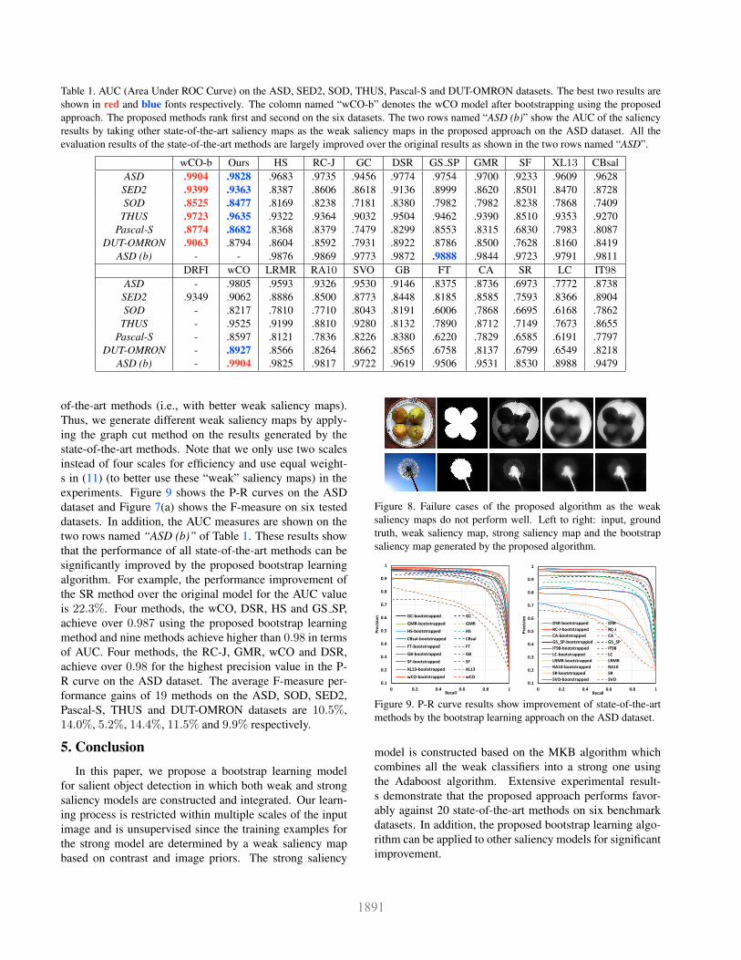
Table 1. AUC (Area Under ROC Curve) on the ASD, SED2, SOD, THUS, Pascal-S and DUT-OMRON datasets. The best two results are
shown in red and blue fonts respectively. The colomn named “wCO-b” denotes the wCO model after bootstrapping using the proposed
approach. The proposed methods rank first and second on the six datasets. The two rows named “ASD (b)” show the AUC of the saliency
results by taking other state-of-the-art saliency maps as the weak saliency maps in the proposed approach on the ASD dataset. All the
evaluation results of the state-of-the-art methods are largely improved over the original results as shown in the two rows named “ASD”.
wCO-b Ours HS RC-J GC DSR GS SP GMR SF XL13 CBsal
ASD .9904 .9828 .9683 .9735 .9456 .9774 .9754 .9700 .9233 .9609 .9628
SED2 .9399 .9363 .8387 .8606 .8618 .9136 .8999 .8620 .8501 .8470 .8728
SOD .8525 .8477 .8169 .8238 .7181 .8380 .7982 .7982 .8238 .7868 .7409
THUS .9723 .9635 .9322 .9364 .9032 .9504 .9462 .9390 .8510 .9353 .9270
Pascal-S .8774 .8682 .8368 .8379 .7479 .8299 .8553 .8315 .6830 .7983 .8087
DUT-OMRON .9063 .8794 .8604 .8592 .7931 .8922 .8786 .8500 .7628 .8160 .8419
ASD (b) - - .9876 .9869 .9773 .9872 .9888 .9844 .9723 .9791 .9811
DRFI wCO LRMR RA10 SVO GB FT CA SR LC IT98
ASD - .9805 .9593 .9326 .9530 .9146 .8375 .8736 .6973 .7772 .8738
SED2 .9349 .9062 .8886 .8500 .8773 .8448 .8185 .8585 .7593 .8366 .8904
SOD - .8217 .7810 .7710 .8043 .8191 .6006 .7868 .6695 .6168 .7862
THUS - .9525 .9199 .8810 .9280 .8132 .7890 .8712 .7149 .7673 .8655
Pascal-S - .8597 .8121 .7836 .8226 .8380 .6220 .7829 .6585 .6191 .7797
DUT-OMRON - .8927 .8566 .8264 .8662 .8565 .6758 .8137 .6799 .6549 .8218
ASD (b) - .9904 .9825 .9817 .9722 .9619 .9506 .9531 .8530 .8988 .9479
of-the-art methods (i.e., with better weak saliency maps).
Thus, we generate different weak saliency maps by apply-
ing the graph cut method on the results generated by the
state-of-the-art methods. Note that we only use two scales
instead of four scales for efficiency and use equal weight-
s in (11) (to better use these “weak” saliency maps) in the
experiments. Figure 9 shows the P-R curves on the ASD
dataset and Figure 7(a) shows the F-measure on six tested
datasets. In addition, the AUC measures are shown on the
two rows named “ASD (b)” of Table 1. These results show
that the performance of all state-of-the-art methods can be
significantly improved by the proposed bootstrap learning
algorithm. For example, the performance improvement of
the SR method over the original model for the AUC value
is 22.3%. Four methods, the wCO, DSR, HS and GS SP,
achieve over 0.987 using the proposed bootstrap learning
method and nine methods achieve higher than 0.98 in terms
of AUC. Four methods, the RC-J, GMR, wCO and DSR,
achieve over 0.98 for the highest precision value in the P-
R curve on the ASD dataset. The average F-measure per-
formance gains of 19 methods on the ASD, SOD, SED2,
Pascal-S, THUS and DUT-OMRON datasets are 10.5%,
14.0%, 5.2%, 14.4%, 11.5% and 9.9% respectively.
5. Conclusion
In this paper, we propose a bootstrap learning model
for salient object detection in which both weak and strong
saliency models are constructed and integrated. Our learn-
ing process is restricted within multiple scales of the input
image and is unsupervised since the training examples for
the strong model are determined by a weak saliency map
based on contrast and image priors. The strong saliency
Figure 8. Failure cases of the proposed algorithm as the weak
saliency maps do not perform well. Left to right: input, ground
truth, weak saliency map, strong saliency map and the bootstrap
saliency map generated by the proposed algorithm.
1 0.998985 0.995833 0.988996 0.978742 0.967646 0.958339
0.198502 0.220614 0.311115 0.462189 0.588434 0.669275 0.722714 0.760505
1 0.956859 0.932825 0.915226 0.901242 0.889679 0.879479 0.870624
0.198502 0.529796 0.636434 0.689749 0.7209 0.74431 0.764197 0.779962
1 0.998944 0.996054 0.988925 0.978857 0.969766 0.962073 0.955956
0.198502 0.220623 0.312355 0.473508 0.615801 0.705122 0.761417 0.800181
1 0.971362 0.958368 0.947988 0.939012 0.930239 0.922293 0.913841
0.198502 0.596668 0.689279 0.745228 0.784004 0.811859 0.833464
1 0.999971 0.999263 0.996502 0.992816 0.988713 0.984211 0.979515
0.198502 0.216807 0.290608 0.413276 0.530211 0.614287 0.67956
1 0.991373 0.984814 0.978828 0.972422 0.966175 0.959811 0.952779
0.198502 0.34036 0.420089 0.487547 0.546427 0.598013 0.640131 0.677577
1 0.9998 0.9985 0.995489 0.990313 0.984006 0.977842 0.971123
0.198502 0.212996 0.273305 0.381449 0.490964 0.579066 0.646069 0.699272
1 0.996639 0.993223 0.988612 0.983668 0.978369 0.972685 0.965954
0.198502 0.275404 0.340007 0.39482 0.444039 0.493797 0.542221 0.582563
1 0.999433 0.996985 0.990381 0.978753 0.964858 0.950376 0.935476
0.198502 0.210841 0.261313 0.340034 0.41977 0.488011 0.545337 0.593391
1 0.96539 0.92304 0.881957 0.841839 0.801431 0.761542 0.722546
0.198502 0.264398 0.34321 0.411997 0.473571 0.522639 0.565179 0.602751
1 0.999914 0.999464 0.998457 0.996573 0.99367 0.989936
0.198502 0.203947 0.224206 0.266502 0.318258 0.363659 0.403125 0.439844
1 0.999299 0.996734 0.992776 0.98805 0.981953 0.974305 0.965352
0.198502 0.236202 0.272545 0.302544 0.328963 0.353891 0.377825 0.401033
1 0.998672 0.994693 0.985401 0.96569 0.941913 0.923739 0.909219
0.1
0.2
0.3
0.4
0.5
0.6
0.7
0.8
0.9
1
0 0.2 0.4 0.6 0.8 1
Pre
cisi
on
Recall
GC-bootstrapped GC
GMR-bootstrapped GMR
HS-bootstrapped HS
CBsal-bootstrapped CBsal
FT-bootstrapped FT
GB-bootstrapped GB
SF-bootstrapped SF
XL13-bootstrapped XL13
wCO-bootstrapped wCO
1 0.999605 0.997566 0.993717 0.987887 0.98121 0.975035 0.969362
0.198502 0.218252 0.304875 0.460966 0.597131 0.674241 0.725753 0.764029
1 0.982384 0.97312 0.964101 0.95479 0.945668 0.936532 0.927745
0.198502 0.614823 0.679576 0.718003 0.745381 0.765974 0.782669 0.797484
1 0.999695 0.998718 0.996238 0.992838 0.989672 0.98615 0.981912
0.198502 0.216012 0.286274 0.405711 0.517404 0.596888 0.659366
1 0.989102 0.98598 0.982513 0.978928 0.974681 0.970165 0.965189
0.198502 0.409187 0.461513 0.51417 0.561826 0.602324 0.637095 0.669028
1 0.999616 0.998387 0.995843 0.991717 0.986935 0.981443 0.975838
0.198502 0.205368 0.230541 0.270983 0.31678 0.359809 0.399964 0.436634
1 0.997455 0.992517 0.985509 0.975782 0.962913 0.947228 0.928877
0.198502 0.228139 0.260025 0.290259 0.31854 0.344854 0.369555 0.392639
1 0.999397 0.99857 0.996914 0.994967 0.992583 0.989925 0.986518
0.198502 0.220225 0.28606 0.399811 0.515489 0.596625 0.654776 0.700652
1 0.988088 0.984873 0.982108 0.978837 0.97597 0.973555 0.970536
0.198502 0.445325 0.494336 0.533049 0.567411 0.598715 0.627108 0.652996
1 0.999512 0.998059 0.995498 0.991745 0.986766 0.980849 0.974396
0.198502 0.205944 0.233525 0.280116 0.330367 0.372913 0.410582 0.445527
1 0.998419 0.995459 0.990654 0.983804 0.974234 0.961022 0.944978
0.198502 0.240503 0.276504 0.307885 0.335606 0.361047 0.384458 0.406513
1 0.99741 0.989466 0.974851 0.954313 0.931797 0.910382 0.890669
0.198502 0.210601 0.250018 0.308412 0.366721 0.418483 0.463138 0.500718
1 0.896744 0.84615 0.806577 0.771966 0.741939 0.714665 0.689201
0.198502 0.25991 0.304303 0.341013 0.374589 0.402885 0.427825 0.450075
1 0.999984 0.999724 0.998759 0.996396 0.992555 0.98836 0.983684
0.1
0.2
0.3
0.4
0.5
0.6
0.7
0.8
0.9
1
0 0.2 0.4 0.6 0.8 1
Pre
cisi
on
Recall
DSR-bootstrapped DSR
RC-J-bootstrapped RC-J
CA-bootstrapped CA
GS_SP-bootstrapped GS_SP
IT98-bootstrapped IT98
LC-bootstrapped LC
LRMR-bootstrapped LRMR
RA10-bootstrapped RA10
SR-bootstrapped SR
SVO-bootstrapped SVO
Figure 9. P-R curve results show improvement of state-of-the-art
methods by the bootstrap learning approach on the ASD dataset.
model is constructed based on the MKB algorithm which
combines all the weak classifiers into a strong one using
the Adaboost algorithm. Extensive experimental result-
s demonstrate that the proposed approach performs favor-
ably against 20 state-of-the-art methods on six benchmark
datasets. In addition, the proposed bootstrap learning algo-
rithm can be applied to other saliency models for significant
improvement.
Acknowledgements. N. Tong and H. Lu are supported by
the Natural Science Foundation of China #61472060 and
the Fundamental Research Funds for the Central Universi-
ties under Grant DUT14YQ101. M.-H. Yang is supported in
part by NSF CAREER Grant #1149783 and NSF IIS Grant
#1152576.
References
[1] R. Achanta, S. Hemami, F. Estrada, and S. Susstrunk.
Frequency-tuned salient region detection. In CVPR, 2009.
1, 5, 6[2] R. Achanta, A. Shaji, K. Smith, A. Lucchi, P. Fua, and
S. Susstrunk. Slic superpixels. EPFL, 2010. 3[3] S. Alpert, M. Galun, R. Basri, and A. Brandt. Image seg-
mentation by probabilistic bottom-up aggregation and cue
integration. In CVPR, 2007. 5[4] F. R. Bach, G. R. Lanckriet, and M. I. Jordan. Multiple kernel
learning, conic duality, and the SMO algorithm. In ICML,
2004. 4[5] A. Borji, D. N. Sihite, and L. Itti. Salient object detection: A
benchmark. In ECCV, 2012. 3[6] Y. Boykov and V. Kolmogorov. An experimental comparison
of min-cut/max-flow algorithms for energy minimization in
vision. PAMI, 26(9):1124–1137, 2004. 4[7] Y. Boykov, O. Veksler, and R. Zabih. Fast approximate en-
ergy minimization via graph cuts. PAMI, 23(11):1222–1239,
2001. 3[8] K.-Y. Chang, T.-L. Liu, H.-T. Chen, and S.-H. Lai. Fusing
generic objectness and visual saliency for salient object de-
tection. In ICCV, 2011. 1, 5[9] M. Cheng, N. J. Mitra, X. Huang, P. H. S. Torr, and
S. Hu. Global contrast based salient region detection. PAMI,
37(3):569–582, 2015. 5, 6[10] M.-M. Cheng, J. Warrell, W.-Y. Lin, S. Zheng, V. Vineet, and
N. Crook. Efficient salient region detection with soft image
abstraction. In ICCV, 2013. 2, 5, 6[11] S. Goferman, L. Zelnik-Manor, and A. Tal. Context-aware
saliency detection. In CVPR, 2010. 5[12] J. Harel, C. Koch, and P. Perona. Graph-based visual salien-
cy. In NIPS, 2006. 1, 2, 5[13] K. He, J. Sun, and X. Tang. Guided image filtering. In ECCV,
2010. 5[14] K. He, J. Sun, and X. Tang. Single image haze removal using
dark channel prior. PAMI, 33(12):2341–2353, 2011. 3[15] X. Hou and L. Zhang. Saliency detection: A spectral residual
approach. In CVPR, 2007. 1, 5[16] L. Itti, C. Koch, and E. Niebur. A model of saliency-based
visual attention for rapid scene analysis. PAMI, 20:1254–
1259, 1998. 2, 5[17] B. Jiang, L. Zhang, H. Lu, C. Yang, and M.-H. Yang. Salien-
cy detection via absorbing markov chain. In ICCV, 2013.[18] H. Jiang, J. Wang, Z. Yuan, T. Liu, N. Zheng, and S. Li.
Automatic salient object segmentation based on context and
shape prior. In BMVC, 2011. 1, 2, 3, 5[19] H. Jiang, J. Wang, Z. Yuan, Y. Wu, N. Zheng, and S. Li.
Salient object detection: A discriminative regional feature
integration approach. In CVPR, 2013. 1, 2, 4, 5[20] D. A. Klein and S. Frintrop. Center-surround divergence of
feature statistics for salient object detection. In ICCV, 2011.
1[21] V. Kolmogorov and R. Zabin. What energy functions can be
minimized via graph cuts? PAMI, 26(2):147–159, 2004. 3[22] B. Kuipers and P. Beeson. Bootstrap learning for place
recognition. In AAAI, 2002. 1[23] X. Li, H. Lu, L. Zhang, X. Ruan, and M.-H. Yang. Salien-
cy detection via dense and sparse reconstruction. In ICCV,
2013. 1, 5, 6[24] Y. Li, X. Hou, C. Koch, J. Rehg, and A. Yuille. The secrets
of salient object segmentation. In CVPR, 2014. 5[25] T. Liu, J. Sun, N.-N. Zheng, X. Tang, and H.-Y. Shum.
Learning to detect a salient object. In CVPR, 2007. 3, 5[26] V. Movahedi and J. H. Elder. Design and perceptual vali-
dation of performance measures for salient object segmenta-
tion. In POCV, 2010. 5[27] T. Ojala, M. Pietikainen, and T. Maenpaa. Multiresolution
gray-scale and rotation invariant texture classification with
local binary patterns. PAMI, 24(7):971–987, 2002. 3[28] F. Perazzi, P. Krahenbuhl, Y. Pritch, and A. Hornung. Salien-
cy filters: Contrast based filtering for salient region detec-
tion. In CVPR, 2012. 1, 2, 5, 6[29] E. Rahtu, J. Kannala, M. Salo, and J. Heikkila. Segmenting
salient objects from images and videos. In ECCV, 2010. 2, 5[30] X. Shen and Y. Wu. A unified approach to salient object
detection via low rank matrix recovery. In CVPR, 2012. 2,
5, 6[31] J. Sun, H. Lu, and S. Li. Saliency detection based on inte-
gration of boundary and soft-segmentation. In ICIP, 2012.[32] N. Tong, H. Lu, L. Zhang, and X. Ruan. Saliency detection
with multi-scale superpixels. SPL, 21(9):1035–1039, 2014.[33] N. Tong, H. Lu, Y. Zhang, and X. Ruan. Salient objec-
t detection via global and local cues. Pattern Recognition,
doi:10.1016/j.patcog.2014.12.005, 2014.[34] Y. Wei, F. Wen, W. Zhu, and J. Sun. Geodesic saliency using
background priors. In ECCV, 2012. 2, 5, 6[35] Y. Xie and H. Lu. Visual saliency detection based on
Bayesian model. In ICIP, 2011. 2[36] Y. Xie, H. Lu, and M.-H. Yang. Bayesian saliency via low
and mid level cues. TIP, 22(5):1689–1698, 2013. 2, 5, 6[37] Q. Yan, L. Xu, J. Shi, and J. Jia. Hierarchical saliency detec-
tion. In CVPR, 2013. 2, 5, 6[38] C. Yang, L. Zhang, H. Lu, X. Ruan, and M.-H. Yang. Salien-
cy detection via graph-based manifold ranking. In CVPR,
2013. 1, 2, 5, 6[39] F. Yang, H. Lu, and Y.-W. Chen. Human tracking by multiple
kernel boosting with locality affinity constraints. In ACCV,
2010. 1, 4[40] J. Yang and M.-H. Yang. Top-down visual saliency via joint
CRF and dictionary learning. In CVPR, 2012. 1, 2[41] Y. Zhai and M. Shah. Visual attention detection in video
sequences using spatiotemporal cues. In ACM MM, 2006. 1,
5[42] L. Zhang, M. H. Tong, T. K. Marks, H. Shan, and G. W. Cot-
trell. Sun: A Bayesian framework for saliency using natural
statistics. Journal of Vision, 8(7), 2008. 1, 2[43] W. Zhu, S. Liang, Y. Wei, and J. Sun. Saliency optimization
from robust background detection. In CVPR, 2014. 1, 2, 5, 6
Related Documents