Salient closed boundary extraction with ratio contour

University of South CarolinaScholar Commons

Faculty Publications Computer Science and Engineering, Departmentof

4-1-2005

Salient Closed Boundary Extraction with RatioContourSong WangUniversity of South Carolina - Columbia, [email protected]

Toshiro Kubota

Jeffrey Mark Siskind

Jun Wang

This Article is brought to you for free and open access by the Computer Science and Engineering, Department of at Scholar Commons. It has beenaccepted for inclusion in Faculty Publications by an authorized administrator of Scholar Commons. For more information, please [email protected].

Publication InfoIEEE Transactions on Pattern Analysis and Machine Intelligence, Volume 27, Issue 4, 2005, pages 546-561.http://ieeexplore.ieee.org/xpl/RecentIssue.jsp?punumber=34© 2005 by the Institute of Electrical and Electronics Engineers (IEEE)

Salient Closed BoundaryExtraction with Ratio ContourSong Wang, Member, IEEE, Toshiro Kubota, Member, IEEE,

Jeffrey Mark Siskind, Member, IEEE, and Jun Wang

Abstract—We present ratio contour, a novel graph-based method for extracting salient closed boundaries from noisy images. This

method operates on a set of boundary fragments that are produced by edge detection. Boundary extraction identifies a subset of these

fragments and connects them sequentially to form a closed boundary with the largest saliency. We encode the Gestalt laws of

proximity and continuity in a novel boundary-saliency measure based on the relative gap length and average curvature when

connecting fragments to form a closed boundary. This new measure attempts to remove a possible bias toward short boundaries. We

present a polynomial-time algorithm for finding the most-salient closed boundary. We also present supplementary preprocessing steps

that facilitate the application of ratio contour to real images. We compare ratio contour to two closely related methods for extracting

closed boundaries: Elder and Zucker’s method based on the shortest-path algorithm and Williams and Thornber’s method based on

spectral analysis and a strongly-connected-components algorithm. This comparison involves both theoretic analysis and experimental

evaluation on both synthesized data and real images.

Index Terms—Image segmentation, perceptual organization, boundary detection, edge detection, graph models.

�

1 INTRODUCTION

IN this paper, we present and analyze a novel method forextracting perceptually salient closed boundaries in

images. This problem can be divided into two parts:formulating appropriate criteria for salience that reflecthuman perceptual judgment and, subsequently, findingboundaries that meet those criteria. Cognitive scientistshave articulated Gestalt laws, such as closure, proximity, andcontinuity, that attempt to characterize boundary salience. Inthis paper, we present one way of formalizing these laws interms of a precise mathematical objective function to beoptimized. We then present a novel graph-theoretic algo-rithm, called ratio contour, for finding a global optimum tothis objective function in polynomial time. Our methodsalways yield closed boundaries and our saliency measure islargely insensitive to boundary length.

The earliest attempts at finding salient boundaries werebased on edgedetection (e.g. [45], [41], [55], [7], [43], [26], [24],[6], [32]). However, suchmethods usually produce boundaryfragments that are not connected into closed boundaries,especially in the presence of noise and occlusion. Further-more, most edge detectors do not incorporate a saliencemetric that reflects the Gestalt laws of proximity andcontinuity. Edge-linking methods, such as [23], attempt toaddress these problems by connecting boundary fragmentsinto closed boundaries using local-search techniques. How-ever, these methods do not guarantee an optimal solution toan independently specified salience measure.

A broader class of local optimization techniques havebeen applied to the general problem of boundary extraction.These include active-contour (e.g., [30], [3], [9], [63], [8], [67])and shape-deformation (e.g., [57], [11], [28], [47], [36], [22])methods. Both types of method usually force the boundaryto be smooth and closed by iteratively updating an initialboundary to produce a series of boundaries that better meetthe saliency criteria. However, the result of such an iterativemethod can depend on the initial boundary and there is noguarantee that a globally optimal boundary will be found.Other approaches for extracting boundaries include theIsing model [46], the Cartoon model [20], the Theater-Wingmodel [39], the Spectrogram model [35], and the Region-Competition model [68], where the saliency measure isexplicitly formulated as a Bayesian variational problem.However, it is usually difficult to find optimal solutions forthese variational problems. In fact, many of these problemsare NP-hard. Practical approaches to solving these problemsoften use local-search techniques that require some form ofinitialization.

To avoid dependence on initialization, graph-theoreticapproaches were introduced to guarantee production ofboundaries that globally optimize a given saliency measure.These methods typically construct a graph where thevertices represent pixels or small regions and the weightededges represent affinity between these pixels or regions. Inthis context, finding a boundary is reduced to the problem ofpartitioning the graph in a way that optimizes some costfunction. Different graph-theoretic methods employ differ-ent algorithms to optimize different cost functions. Theseinclude Minimum Cut [66], Ratio Regions [13], NormalizedCut [54], Average Cut [49], the methods of Jermyn andIshikawa [29], Ratio Cut [61], and many more recentmethods (e.g., [40], [19], [51], [59], [52], [56], [5], [18]). Someof these methods attempt to solve NP-hard problems usingapproximate algorithms. Because many of those methodsconstruct graphs where vertices correspond to pixels orsmall regions, it is difficult to incorporate many Gestalt laws,

546 IEEE TRANSACTIONS ON PATTERN ANALYSIS AND MACHINE INTELLIGENCE, VOL. 27, NO. 4, APRIL 2005

. S. Wang, T. Kubota, and J. Wang are with the Department of ComputerScience and Engineering, University of South Carolina, Columbia, SC29208. E-mail: {songwang, kubota, wang286}@cse.sc.edu.

. J.M. Siskind is with the School of Electrical and Computer Engineering,465 Northwestern Ave., Room 330, Purdue University, West Lafayette, IN47906. E-mail: [email protected].

Manuscript received 16 Mar. 2004; revised 30 Sept. 2004; accepted 1 Oct.2004; published online 10 Feb. 2005.Recommended for acceptance by R. Basri.For information on obtaining reprints of this article, please send e-mail to:[email protected], and reference IEEECS Log Number TPAMI-0132-0304.

0162-8828/05/$20.00 � 2005 IEEE Published by the IEEE Computer Society

such as smoothness, into the formulation of the saliencymeasure.

Cost functions that measure the Gestalt properties ofclosure, proximity, and continuity can be more conveni-ently formulated in terms of preextracted boundaryfragments than image pixels. These boundary fragments,or simply fragments,1 can be obtained with an edgedetector. In this context, boundaries are extracted byidentifying and connecting a subset of these fragmentsinto a salient boundary. The Gestalt laws correspond toenforcing specified properties of a boundary. Closurerequires that the boundary be a cycle. Proximity requiresthe gap between two neighboring fragments to be small.Continuity requires the resulting boundary to be smooth.Methods have been proposed for connecting fragments in away that attempts to satisfy these properties (e.g., [53], [16],[37], [2], [27], [48], [21], [64], [4], [65], [37], [25], [4], [27],[44]). These methods typically:

1. Define a prominence2 measure for each fragment and/or gap between two neighboring fragments. Thismeasure is usually based on the smoothness andlength of these fragments and/or gaps to encode thelocal continuity and proximity properties.

2. Define a saliency measure for valid boundaries interms of fragment and gap prominence definedabove. For example, saliency of a boundary can bedefined as the sum of the prominences of itscomponent fragments and gaps.

3. Develop an optimization algorithm for finding theboundary that maximizes the selected saliencymeasure. Such algorithms may employ graph-theoretic techniques in an attempt to achieve globaloptimality [16], [37].

Prior methods differ in their choice of prominence andsaliency measures and approaches to optimization.

A psychological study has shown that boundary closureplays a critical role in human perception, as shown byKovacs and Julesz [33, p. 7496]:

We found an unexpected advantage of circular arrangements: �c

(maximum spacing for closed contours) was extended by a factor of1.8 relative to �o (maximum spacing for open ones).

In other words, with similar maximum gap (spacing)between fragments, humans may perceive closed curves,but not open ones. The maximum allowed gap in perceivinga closed curve is 1.8 times the maximum allowed gap inperceiving an open curve. Since closure appears to beimportant in human vision, researchers deem it prudent toincorporate closure into computer vision.

As a global property, boundary closure is usually moredifficult to enforce with prominence measures than localproperties such as proximity and continuity. In fact, many ofthe above methods cannot guarantee production of closedboundaries. One way to enforce closure is to performconstrained optimization that only considers closed bound-aries. In the context of graph-based optimization algorithms,this constraint corresponds to finding cycles in a graph. For

example, Elder and Zucker [16] define boundary saliency asthe product of fragment/gap prominence along the bound-ary and then use the shortest-path algorithm [14] to find theoptimal cycle. Similarly, Williams and Thornber [65] defineboundary saliency as the geometric mean of fragment/gapprominence along the boundary and use spectral-analysistechniques to enhance the fragment/gap prominencemeasure with closure information.3 With this measure,Mahamud et al. [37] attempt to enforce closure using astrongly-connected-components algorithm [12]. Other re-lated methods that attempt to find closed boundariesinclude [27], [4], [42].

This paper presents a new graph-based method, calledratio contour, for detecting closed salient boundaries, wherethe globally most-salient boundary is found in polynomialtime. Like the methods described above, ratio contour findsboundaries by identifying and connecting a set of preex-tracted fragments. Further, ratio contour guarantees closureby constrained graph-based optimization. We encode theGestalt laws of proximity and continuity in a novelboundary-saliency measure based on relative gap lengthand average curvature. Formulating saliency in terms ofrelative gap length and average curvature removes the biastoward short boundaries that is present in saliencymeasures based on total gap length and curvature.

Our paper contains two major parts. In the first part, wepresent the algorithmic details of ratio contour along withthe supplementary processing steps needed to use thismethod to extract salient boundaries from images. Morespecifically, we present methods for 1) preprocessing theedge-detector output to produce a set of topologicallyunconnected fragments, 2) smoothing the detected frag-ments to remove noise, and 3) reliably estimating thecurved gap-filling segment between two detected frag-ments. The latter two use a spline-based curve smoothingalgorithm for noise removal and robust gap filling. In thesecond part, we analyze the differences between ratiocontour and the two most-related prior methods: Elder andZucker (EZ) [16] and Williams and Thornber (WT) [65], [37],and compare their performance on synthesized and realimages in a unified framework.

The remainder of this paper is organized as follows:Section 2 formulates the saliency measure used by ratiocontour and converts the problem of finding the most-salient boundary with this measure into the problem offinding an optimal cycle in a graph. Section 3 presents apolynomial-time algorithm for finding the desired optimalcycles. Section 4 discusses the preprocessing steps 1) through3) described above to derive the fragment/gap prominencemeasure, in terms of graph edge weights, from noisy edge-detector output. Section 5 illustrates the boundariesdetected by ratio contour on real images. Section 6 analyzesthe similarities and differences between ratio contour andthe methods of EZ and WT. Section 7 compares theperformance of ratio contour with that of EZ and WT withexperiments on real and synthetic images. Section 8concludes with a summary of our method.

2 PROBLEM FORMULATION

We refer to the process of identifying a subset of fragmentsproduced by preprocessing and connecting the fragments inthat subset to form a closed boundary as boundary extraction.

WANG ET AL.: SALIENT CLOSED BOUNDARY EXTRACTION WITH RATIO CONTOUR 547

1. Prior literature often uses the term “edge” instead of “fragment.” Wedo not use this terminology to avoid confusion with the notion of edge in itsgraph-theoretic sense.

2. Note that we have prominence measures for both fragments and gaps.Prior literature often uses the term “affinity” between a pair of fragments torefer to what we call gap prominence. We refrain from using the termaffinity as it is not appropriate for individual fragments and we wish to useunified terminology for both fragments and gaps.

3. In [37], such enhanced fragment/gap prominence is referred to as“edge saliency” and “link saliency.”

As shown in Fig. 1a, the input to boundary extractionconsists of a set of noncrossing fragments, each of which is acontinuous open curve segment with two endpoints. Wefurther assume that a boundary produced by boundaryextraction always consists of indivisible fragments, i.e., aboundary cannot contain only part of a fragment. The goalof boundary extraction is to find the closed boundary withmaximum perceptual saliency, as shown in Fig. 1b. To forma closed boundary from disconnected fragments, weconstruct another set of fragments to fill the gaps betweenthe initial fragments. To distinguish these two kinds offragments, we refer to the initial fragments, the solid curvesin Fig. 1b, as real fragments and the gap-filling fragments,the dashed curves in Fig. 1b, as virtual fragments.

Virtual fragments are derived from adjacent real frag-ments by a process of gap completion. Any gap-completionmethod can be used (e.g., [38], [58], [64], [51]). For theexperiments in this paper, we use the particular gap-completion method that we present in Section 4. Weassociate a prominence or fragment cost with each fragmentto describe how likely or unlikely that fragment is to beincluded in the most-salient boundary. Such fragmentprominence or cost usually incorporates only local informa-tion derived from a given fragment. Many formulations offragment prominence or cost have been proposed (e.g., [16],[64], [60]). Such formulations often attempt to codify theGestalt laws of proximity and continuity: 1) real fragmentsare more prominent than virtual fragments, 2) short virtualfragments are more prominent than long virtual fragments,and 3) smooth fragments are more prominent thannonsmooth fragments.

A closed boundary can then be constructed by connect-ing a subset of real and virtual fragments, sequentially andalternately, as shown in Fig. 1b. We are only interested innondegenerate boundaries where no fragment is traversedmore than once when forming a closed boundary. For theremainder of the paper, we use the term “boundary,”without the qualifier “degenerate,” to refer to nondegene-rate boundaries. Note that the nondegeneracy of aboundary does not require it to be non-self-crossing4 inour problem formulation because a virtual fragment maycross another real or virtual fragment along an extractedboundary. An example of this is shown in Fig. 1c, where theboundary is nondegenerate but self crossing. The ratio-contour method presented in this paper extracts onlynondegenerate boundaries, which, however, may be self-crossing. Associated with each closed boundary, we candefine a boundary saliency Sð�Þ or a boundary cost �ð�Þ as a

function of the prominence or cost of the fragments thatform that boundary. Finally, we develop an optimizationalgorithm to search for a closed boundary that maximizesthis boundary saliency or, alternatively, minimizes theboundary cost. In essence, various boundary-extractionmethods differ mainly in their definition of boundarysaliency/cost and/or their optimization algorithm.

We encode the Gestalt laws of proximity and continuityinto the following boundary-cost definition:

�rcðBÞ ¼4 WðBÞ

LðBÞ ¼RB½�ðtÞ þ � � �2ðtÞ�dtR

B dt; ð1Þ

where vðtÞ, 0 � t � LðBÞ, is the arc-length parameterizedform of the boundary B, �ðtÞ ¼ 1 if the point vðtÞ is in avirtual fragment, �ðtÞ ¼ 0 if it is in a real fragment, and �ðtÞis the curvature of the boundary at vðtÞ. The most-salientboundary B is then the one with the minimum cost �rcðBÞ.The cost �rcðBÞ normalizes WðBÞ, a weighted sum of thetotal gap-length and curvature along the boundary B, byLðBÞ, the length of the boundary B, in an attempt to removea possible bias toward short boundaries in WðBÞ. Theparameter � > 0 controls the relative contribution ofproximity and continuity to this cost.

While �rc avoids a bias toward short boundaries, it doesnot eliminate all biases dependent on boundary length. Thechoice of most-salient boundary using �rc can depend onimage scale, given a fixed �. An example is shown in Fig. 2,which contains two circular boundaries, A and B. Along A,the virtual fragments count for half of the boundary length,while, along B, the virtual fragments count for one-third ofthe boundary length. Consider the case where the radius ofthese two circular boundaries are rA ¼ 4 and rB ¼ 2 and� ¼ 2. It is easy to see that

�rcðAÞ ¼1

2þ �

r2A¼ 1

2þ 1

8< �rcðBÞ ¼

1

3þ �

r2B¼ 1

3þ 1

2;

548 IEEE TRANSACTIONS ON PATTERN ANALYSIS AND MACHINE INTELLIGENCE, VOL. 27, NO. 4, APRIL 2005

Fig. 1. Extracting a salient boundary from a set of fragments. (a) Real fragments. (b) A nondegenerate non-self-crossing closed boundary derived byconnecting a subset of real and virtual fragments. (c) A nondegenerate self-crossing closed boundary. (d) The solid-dashed graph G constructedfrom (a) together with a simple alternate cycle (shown in thick lines) corresponding to the boundary shown in (b). (e) A simple alternate cycle (shownin thick lines) corresponding to the boundary shown in (c).

4. Prior literature often refers to non-self-crossing boundaries as“simple” boundaries. We do not use this terminology to avoid confusionwith the notion of simple cycles in a graph.

Fig. 2. The most-salient boundary that optimizes �rc can depend on

image scale and the parameter �.

i.e., A is more salient than B. If we enlarge the image by a

factor of 2, we have rA ¼ 8 and rB ¼ 4. With the same � ¼ 2,

we have

�rcðAÞ ¼1

2þ �

r2A¼ 1

2þ 1

32> �rcðBÞ ¼

1

3þ �

r2B¼ 1

3þ 1

8;

i.e., B is more salient than A.The parameter � > 0 specifies the relative contribution of

proximity and continuity to saliency. With smaller �,proximity dominates. With larger �, continuity or smooth-ness dominates. Therefore, different values for � may leadto different most-salient boundaries. To see this, consideragain the two circular boundaries shown in Fig. 2 with theradii rA ¼ 4 and rB ¼ 2. We have previously shown thatwith � ¼ 2, A is more salient than B. However, with � ¼ 0:5,we have

�rcðAÞ ¼1

2þ �

r2A¼ 1

2þ 1

32> �rcðBÞ ¼

1

3þ �

r2B¼ 1

3þ 1

8;

i.e., B is more salient than A. Finding an optimal � for aninput image is one of our ongoing research topics. In thispaper, we choose a fixed � for all experiments.

We now formulate the problem of boundary extractioninto an optimization problem in an undirected graphG ¼ ðV ;EÞ. We construct a unique vertex for each fragmentendpoint. Two kinds of edges, solid and dashed, are thenconstructed between vertices to represent real and virtualfragments, respectively. An example of such a graph isshown in Fig. 1d. This graph is constructed from the realfragments in Fig. 1a and consists of seven solid edges and25 dashed edges. To illustrate this construction clearly, thegraph in Fig. 1d is embedded so that each vertex uA has thesame spatial coordinate as its corresponding fragmentendpoint A in Fig. 1a. G must have an even number ofvertices since each real fragment has two endpoints.Furthermore, no two solid edges can be incident on thesame vertex. We call such a graph an (undirected) solid-dashed (SD) graph. In this graph, an alternate cycle is definedas a cycle that alternately traverses solid and dashed edgesand a simple cycle as a cycle that does not traverse a vertexmore than once. For the remainder of the paper, we use theterm “cycle,” without the qualifier “nonsimple,” to refer tosimple cycles. Examples of an SD graph and alternate cyclesare illustrated in Figs. 1d and 1e. It is easy to see thatnondegenerate closed boundaries correspond exactly tosimple alternate cycles in G. Thus, we can constrain ouroptimization of saliency to consider only nondegenerateclosed boundaries by using graph algorithms that findsimple alternate cycles.

To formulate the boundary cost (1) in terms of G, weassociate a weight wðeÞ and a length lðeÞ with each edge e inG. For convenience, we define BðeÞ as the original (real orvirtual) fragment corresponding to an edge e. Based on this,we define

wðeÞ ¼4 W ðBðeÞÞ ¼ZBðeÞ½�ðtÞ þ � � �2ðtÞ�dt; ð2Þ

which is the unnormalized cost of BðeÞ, and

lðeÞ ¼4 LðBðeÞÞ ¼ZBðeÞ

dt; ð3Þ

which is the curve length of BðeÞ. The most-salient closed

boundary B with minimum cost �rcðBÞ corresponds to an

alternate cycle C that minimizes the cycle ratio

�rcðCÞ ¼P

e2C wðeÞPe2C lðeÞ : ð4Þ

In the next section, we present a polynomial-time algorithm

for finding such an optimal alternate cycle.

3 THE RATIO-CONTOUR ALGORITHM

For simplicity, we denote an alternate cycle with minimum

cycle ratio as a Minimum Ratio Alternate (MRA) cycle. In this

section, we introduce a polynomial-time algorithm for

finding an MRA cycle in an SD graph G. This algorithm

consists of three reductions: 1) Reduce the problem of

finding an MRA cycle in a general SD graph G to the

problem of finding an MRA cycle in a special SD graph with

the same structure as G, except that all the solid edges have

zero weight and length. This reduction is achieved by

merging the weight and length of solid edges into the

weight and length of their adjacent dashed edges, without

changing the structure of the graph. 2) Reduce the problem

of finding an MRA cycle in an SD graph G to the problem of

finding a Negative total Weight Alternate (NWA) cycle in the

same graph G. 3) Reduce the problem of finding an NWA

cycle in an SD graph G with zero solid-edge weights and

lengths to the problem of finding a Minimum-Weight Perfect

Matching (MWPM) in the same graph G. One can find an

MWPM in polynomial-time [15]. This allows us to find an

MRA cycle in polynomial time as well.

3.1 Reduction 1: Setting the Weight and Lengthof Solid Edges to Zero

From (2) and (3), the weight and length of any edge in

the constructed SD graph G are usually nonzero. In this

section, we show how to transform the edge weights and

lengths in G so that all solid edges have zero weight and

length without changing the MRA cycle. As illustrated in

Fig. 3, no two solid edges can be adjacent. Therefore, each

solid edge e ¼ ðu; vÞ can only be adjacent to a set of

dashed edges, say fe1; e2; . . . ; eKg, in G. We can decom-

pose the weight wðeÞ and length lðeÞ of the solid edge e

arbitrarily into sums of two nonnegative terms: wðeÞ ¼wuðeÞ þ wvðeÞ and lðeÞ ¼ luðeÞ þ lvðeÞ. We can then reas-

sign the weight and length of the solid edge to its

adjacent dashed edges by the following transformation:

WANG ET AL.: SALIENT CLOSED BOUNDARY EXTRACTION WITH RATIO CONTOUR 549

Fig. 3. Reassigning the weight and length of a solid edge to its adjacentdashed edges. (a) The cases where solid and dashed edges share onlyone vertex. (b) A case where solid and dashed edges share two vertices.

wðekÞ wðekÞþwuðeÞ if ek only shares vertex u with e

wvðeÞ if ek only shares vertex v with e

wðeÞ if ek shares both vertices u and v with e

8><>:lðekÞ lðekÞþ

luðeÞ if ek only shares vertex u with e

lvðeÞ if ek only shares vertex v with e

lðeÞ if ek shares both vertices u and v with e

8><>:

for k ¼ 1; 2; . . . ; K sequentially. We can then reset theweight and length of the solid edge e to zero. For example,we can set wuðeÞ ¼ wvðeÞ ¼ 1

2wðeÞ and luðeÞ ¼ lvðeÞ ¼ 12 lðeÞ to

divide the weight and length of the solid edge e into twoequal components and then reassign these components tothe adjacent dashed edges. This reassignment process isperformed iteratively over all solid edges. Since solid anddashed edges are traversed alternately in an alternate cycle,this process will not change the total weight and length ofany alternate cycle in G. Therefore, this process does notchange the MRA cycle in G.

3.2 Reduction 2: Detecting Negative-WeightAlternate Cycles

In this section, we reduce the problem of finding an MRAcycle in an SD graph G to the problem of finding analternate cycle with negative total edge weight in the samegraph G by searching for an appropriate transformation ofthe edge weights in G that preserves the MRA cycle butwhere the MRA cycle has a cycle ratio of zero. The cost offinding the appropriate parameter b� for this transformationis incorporated into the complexity analysis of the algo-rithm. This reduction is possible because an MRA cycle in Gis invariant to the following linear transformation of theedge weights:

w0ðeÞ ¼ wðeÞ � b � lðeÞ; 8e 2 E: ð5Þ

This holds because, for any two alternate cycles C1 and C2

in G, �rcðC1Þ � �rcðC2Þ implies

�0rcðC1Þ ¼P

e2C1w0ðeÞP

e2C1lðeÞ ¼

Pe2C1½wðeÞ � b � lðeÞ�P

e2C1lðeÞ

¼ �rcðC1Þ � b � �rcðC2Þ � b ¼P

e2C2w0ðeÞP

e2C2lðeÞ

¼ �0rcðC2Þ;

where �0rcð�Þ denotes the cycle ratio after the edge-weighttransformation.

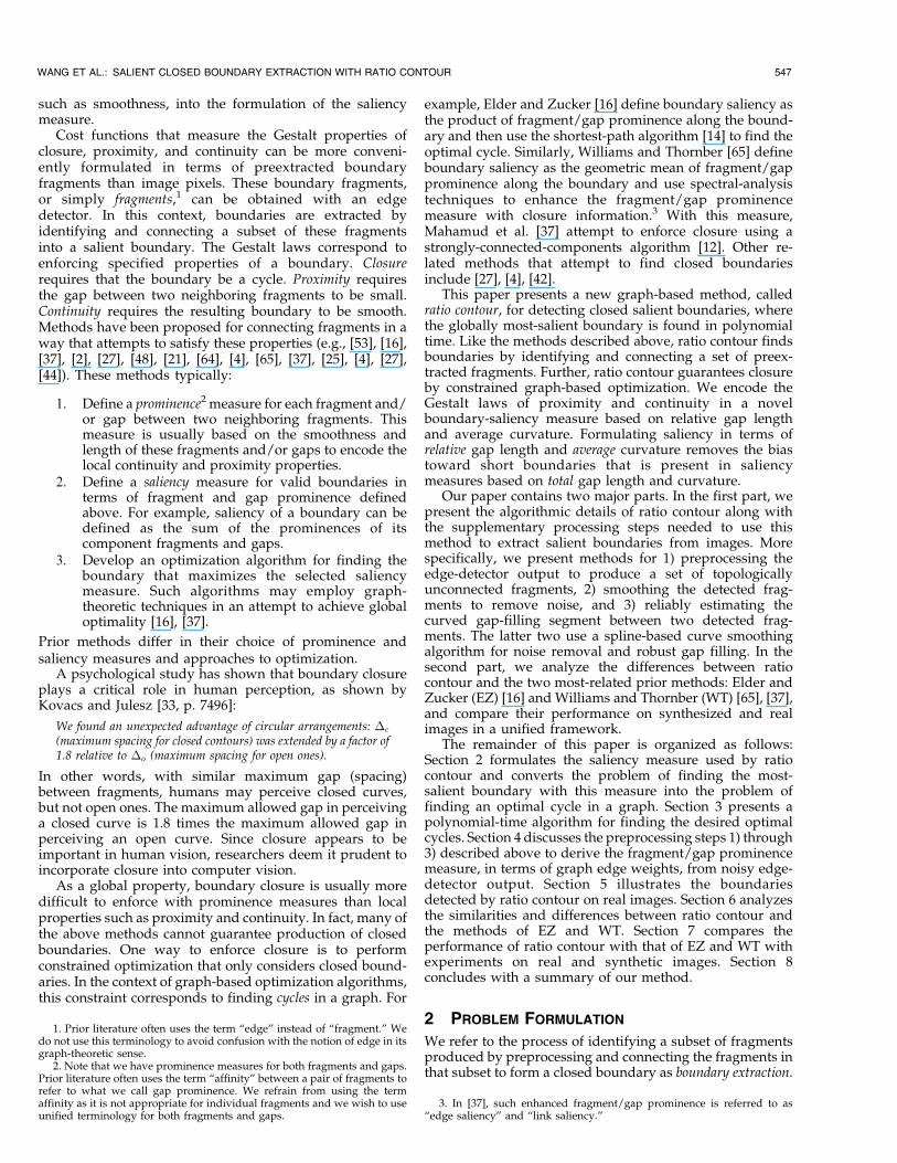
Since edge lengths are nonnegative, there exists anoptimal b ¼ b� so that, after the above edge-weight transfor-mation, the resulting MRA cycles have a cycle ratio of zero.In this case, MRA cycles are the same as the cycles with zerototal edge weight. Now, suppose that we have an NWAcycle-detection algorithm that can determine whether thereis an NWA cycle inG and, if there is, can extract such a cycle,both in polynomial time. Then, we can use this NWA cycle-detection algorithm repeatedly to determine b� using thefollowing sequential-search algorithm, as shown in Fig. 4.

This sequential-search algorithm is adapted from Ahujaet al. [1, pp. 496-497], where it is used for finding aminimum ratio cycle in a directed graph. The correctness ofthis algorithm comes from the fact that an alternate cycle Calways has zero total weight when all the edge weights are

transformed by w0ðeÞ ¼ wðeÞ � �rcðCÞ � lðeÞ, after Step 3. Toavoid confusion, we specify that the cycle ratio �rcðCÞ isalways calculated using the original edge weights in Gwithout applying the edge-weight transformation (5).Furthermore, we know that, with the current edge-weighttransformation w0ðeÞ ¼ wðeÞ � �rcðCÞ � lðeÞ, there is no alter-nate cycle with negative total weight after termination. Thisimplies that after termination b� ¼ �rcðCÞ and the current Cis a desired MRA cycle.

It can be shown that this search process terminates in a(pseudo)polynomial number of iterations if the edgeweightsand lengths are all integers. Let wmax ¼ maxe2E wðeÞ andlmax ¼ maxe2E lðeÞ. The cycle ratio of any alternate cycle Chas the form

�rcðCÞ ¼P

e2C wðeÞPe2C lðeÞ :

When all edge weights and lengths are integral, thenumerator,

Pe2C wðeÞ, can take on at most wmaxjEj different

values. Similarly, the denominator,P

e2C lðeÞ, can take on atmost lmaxjEj different values. Therefore, the cycle ratio�rcðCÞ of any alternate cycle C in G can take on at mostwmaxlmaxjEj2 different values. Notice that, in the abovesequential-search algorithm, the estimated b ¼ �rcðCÞ willstrictly decrease after each iteration. Therefore, this algo-rithm terminates in at most wmaxlmaxjEj2 iterations.

Now, let us consider the combination of the firstreduction described in Section 3.1 and this second reduc-tion. After the first reduction, the SD graph G has a specialproperty: All solid edges have zero weight and length. Theedge-weight transformation (5) preserves this property.Therefore, we need only develop an NWA cycle-detectionalgorithm for SD graphs where all the solid edges have zeroweight and length.

3.3 Reduction 3: Finding Minimum Weight PerfectMatchings

The problem of detecting an NWA cycle in an SD graphwhere all the solid edges have zero weight and length canbe reduced to the problem of finding an MWPM in the samegraph. A perfect matching in G denotes a subgraph of Gthat contains all the vertices in G, but where each vertexonly has one incident edge. Fig. 5a shows an example ofperfect matching where the seven thick edges, together withtheir vertices, form a perfect matching. The MWPM is theperfect matching with minimum total edge weight. In an SDgraph, all the solid edges form a trivial perfect matching,which, in our case, has zero total weight given the firstreduction from Section 3.1. Therefore, the MWPM in our SDgraph will have nonpositive total weight.

We can derive a set of cycles from an MWPM P with thefollowing two-step algorithm:

550 IEEE TRANSACTIONS ON PATTERN ANALYSIS AND MACHINE INTELLIGENCE, VOL. 27, NO. 4, APRIL 2005

Fig. 4. Sequential-search algorithm.

1. Remove from P all the solid edges and their incidentvertices. We denote the resulting graph as P 0.

2. Add the edge e to P 0 if (a) e is a solid edge in G and(b) e is not in the MWPM P . We denote the resultinggraph as P 00.

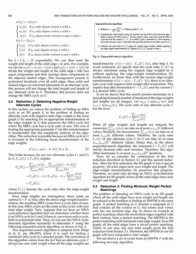
The graph P 00 produced by the above algorithm consists of aset of disjoint alternate cycles because each vertex in P 00 hastwo incident edges: one solid and one dashed. Twoexamples of this reduction are shown in Fig. 5. Since allthe solid edges have zero weight and length and we onlyremove and add solid edges in the above algorithm, thetotal weight of the MWPM P is the same as the total weightof the derived alternate-cycle set P 00. When P 00 contains asingle alternate cycle, as shown in Figs. 5a and 5b, the NWAcycle-detection problem is reduced to the problem offinding an MWPM and checking whether it has negativetotal weight.

However, P 00 may contain multiple alternate cycles, asshown in Figs. 5c and 5d. It is easy to see that at least one ofthese alternate cycles must have nonpositive total weight,for otherwise, the sum of the total weights of all of thealternate cycles would be positive. This is sufficient for ourreduction. We can show an even stronger property;however, each alternate cycle in P 00 must have nonpositivetotal weight. This can be shown by contradiction. Assumeone cycle, Cþ, in the cycle set P 00, has a positive total weight.Then, we can construct a new perfect matching Q from theMWPM P by: 1) removing from P all the dashed edges inCþ and 2) adding into P all solid edges in Cþ. Theconstruction of Q from P is illustrated in Figs. 5c, 5d, and5e. As all the solid edges have zero weight and length, Qmust have less total edge weight than P . This contradictsthe assumption that P is an MWPM. Therefore, even whenP 00 contains multiple alternate cycles, the problem offinding an NWA cycle in G can still be reduced to theproblem of finding an MWPM in G simply by choosingfrom P 00 the cycle with minimum cycle ratio �rcðCÞ (basedon the original edge weights) for the sequential-searchalgorithm from Section 3.2. This cycle brings b closer to thedesired b� than any other cycle in P 00. Although the earlieranalysis provides an upper-bound of wmaxlmaxjEj2 on thenumber of iterations required in the sequential-searchalgorithm from Section 3.2, none of the experimentsreported in the paper requires more than eight iterationsusing this NWA cycle-detection algorithm.

4 FRAGMENT CONSTRUCTION AND EDGE-WEIGHT

FUNCTION

This section discusses the supplementary processing stepsneeded to use the above ratio-contour algorithm to extractsalient boundaries from real images: the construction of thereal and virtual fragments and the calculation of edge

weights and lengths. Specifically, we discuss the followingissues: 1) preprocessing the edge-detector output toproduce a set of topologically unconnected fragments,2) smoothing the detected fragments to remove noise, and3) reliably estimating the curved gap-filling segmentbetween two detected fragments. The latter two use aspline-based curve-smoothing algorithm for noise removaland robust gap filling.

4.1 Preprocessing the Edge-Detector Output

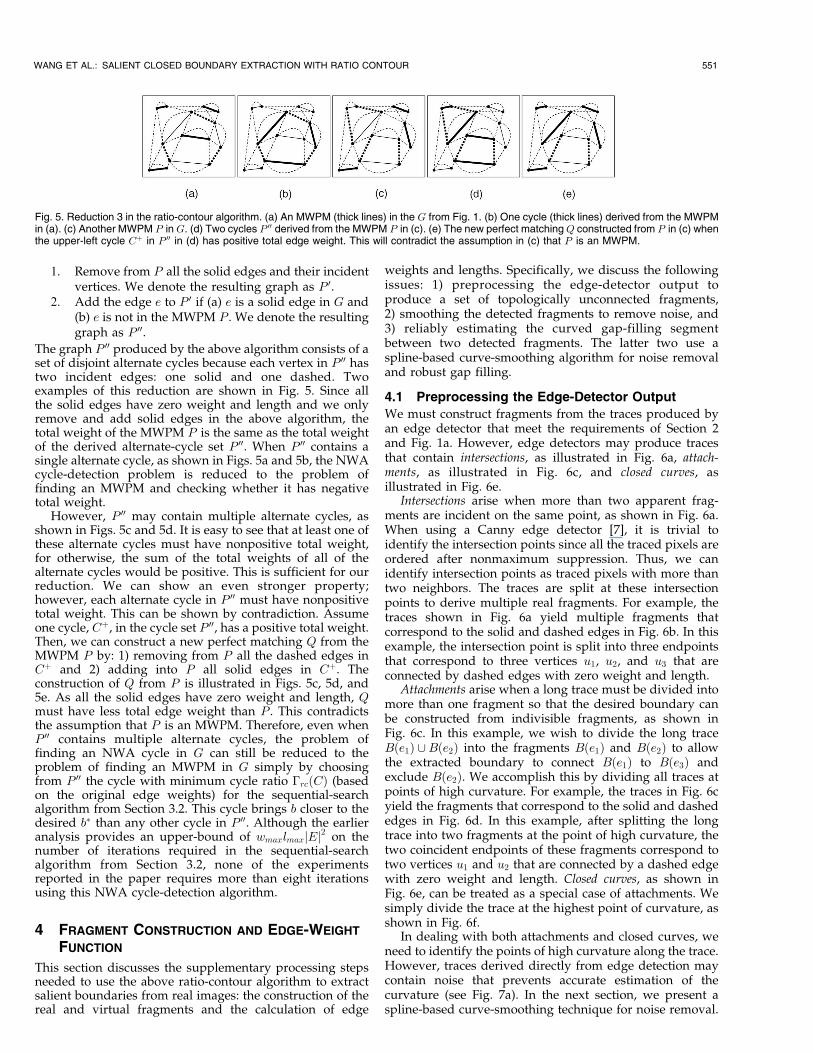
We must construct fragments from the traces produced byan edge detector that meet the requirements of Section 2and Fig. 1a. However, edge detectors may produce tracesthat contain intersections, as illustrated in Fig. 6a, attach-ments, as illustrated in Fig. 6c, and closed curves, asillustrated in Fig. 6e.

Intersections arise when more than two apparent frag-ments are incident on the same point, as shown in Fig. 6a.When using a Canny edge detector [7], it is trivial toidentify the intersection points since all the traced pixels areordered after nonmaximum suppression. Thus, we canidentify intersection points as traced pixels with more thantwo neighbors. The traces are split at these intersectionpoints to derive multiple real fragments. For example, thetraces shown in Fig. 6a yield multiple fragments thatcorrespond to the solid and dashed edges in Fig. 6b. In thisexample, the intersection point is split into three endpointsthat correspond to three vertices u1, u2, and u3 that areconnected by dashed edges with zero weight and length.

Attachments arise when a long trace must be divided intomore than one fragment so that the desired boundary canbe constructed from indivisible fragments, as shown inFig. 6c. In this example, we wish to divide the long traceBðe1Þ [Bðe2Þ into the fragments Bðe1Þ and Bðe2Þ to allowthe extracted boundary to connect Bðe1Þ to Bðe3Þ andexclude Bðe2Þ. We accomplish this by dividing all traces atpoints of high curvature. For example, the traces in Fig. 6cyield the fragments that correspond to the solid and dashededges in Fig. 6d. In this example, after splitting the longtrace into two fragments at the point of high curvature, thetwo coincident endpoints of these fragments correspond totwo vertices u1 and u2 that are connected by a dashed edgewith zero weight and length. Closed curves, as shown inFig. 6e, can be treated as a special case of attachments. Wesimply divide the trace at the highest point of curvature, asshown in Fig. 6f.

In dealing with both attachments and closed curves, weneed to identify the points of high curvature along the trace.However, traces derived directly from edge detection maycontain noise that prevents accurate estimation of thecurvature (see Fig. 7a). In the next section, we present aspline-based curve-smoothing technique for noise removal.

WANG ET AL.: SALIENT CLOSED BOUNDARY EXTRACTION WITH RATIO CONTOUR 551

Fig. 5. Reduction 3 in the ratio-contour algorithm. (a) An MWPM (thick lines) in the G from Fig. 1. (b) One cycle (thick lines) derived from the MWPMin (a). (c) Another MWPM P inG. (d) Two cycles P 00 derived from the MWPM P in (c). (e) The new perfect matchingQ constructed from P in (c) whenthe upper-left cycle Cþ in P 00 in (d) has positive total edge weight. This will contradict the assumption in (c) that P is an MWPM.

4.2 Smoothing the Detected Fragments

To accurately estimate the curvature along a trace, we needto remove noise and aliasing. To accomplish this, weemploy a spline-based smoothing technique that representsa trace by a set of quadratic splines. Note that each trace isoriginally represented by a set of connected pixel pointsextracted by an edge detector. We refer to these pixel pointsas control points and associate a quadratic spline to eachcontrol point that interpolates that control point and itsneighbor. The spline for the ith control point has thefollowing parametric form:

xiðtÞyiðtÞ

� �¼ �xxi

�yyi

� �þ Ai Bi

Ci Di

� �t2

t

� �;

where piðtÞ ¼ ðxiðtÞ; yiðtÞÞT is the spatial coordinate of the ithspline parameterized with t 2 ½�1; 1�, �ppi ¼ ð�xxi; �yyiÞT is thespatial coordinate of the control point and Ai, Bi, Ci, and Di

are the coefficients of the quadratic. We smooth these splinesby visiting each in turn and adjusting its attributes (�xxi, �yyi,Ai,Bi, Ci, andDi) to improve a continuity measure. The processrepeats iteratively until themeasure reaches a given tolerancelevel. Thus, among all the representations whose continuitymeasure is under the tolerance level, the process returns thefirst one to be reached from the original representation by theiterative optimization process [34]. While we cannot provethat such a smoothed fragment remains aligned with theoriginal unsmoothed fragment, in practice, we have neverobserved a case of significant misalignment. Furthermore,with the parametric form of the quadratic splines associatedwith each trace, the total length of the ith spline and thecurvature along that spline can be computed by

li ¼Z 1

0

ffiffiffiffiffiffiffiffiffiffiffiffiffiffiffiffiffiffiffiffiffiffiffiffiffiffiffiffiffiffiffiffiffiffiffiffiffiffiffiffiffiffiffiffiffiffiffiffiffiffiffiffiffiffiffiffiffiffið2AitþBiÞ2 þ ð2CitþDiÞ2

qdt;

�iðtÞ ¼2ðBiCi �AiDiÞ

ðð2AitþBiÞ2 þ ð2CitþDiÞ2Þ3=2:

This can be used to calculate the edge weights and lengthsin the constructed SD graph.

To derive the optimal attributes for these quadraticsplines, we form a prior energy term that penalizesdeviation away from C1 continuities. We use the followingenergy function:

Ep ¼XN�1i¼1

�kpið0Þ � piþ1ð�1Þk2 þ kpið1Þ � piþ1ð0Þk2 þ k _ppið0Þ

� _ppiþ1ð�1Þk2 þ k _ppið1Þ � _ppiþ1ð0Þk2�;

where k � k2 is the L2 norm and _ppðtÞ is the tangent vector at t.The smoothing process iteratively visits each spline sequen-tially toupdate its attributes [34]. This canbeperformedusinga block Gauss-Seidel method. Throughout the experimentspresented in this paper, we iterate the Gauss-Seidel process50 times to smooth each trace.An example of trace smoothingusing this method is shown in Fig. 7.

4.3 Gap Filling

The final supplementary processing step is to derive virtualfragments from the real fragments. One approach is toestimate a virtual fragment that interpolates each pair ofreal-fragment endpoints in a way that satisfies specifiedcontinuity and perceptual criteria. This approach is oftencalled curve completion [21], [50], [31]. For example, Figs. 8aand 8b show a closed boundary and the same boundarywith three gaps, respectively. In the ideal case, we wishcurve completion to derive three virtual fragments to fillthese gaps, as shown in Fig. 8c, and produce a boundarythat resembles the original one in Fig. 8a.

However, curve completion does not work properly withnoisy or aliased real fragments. For example, noise at thefragment endpoints shown in Fig. 8d may result in virtualfragments that deviate significantly from the original curve,as shown in Fig. 8e, because the noisy tangent values atfragment endpoints dominate this curve-completion pro-cess. Real fragments derived by preprocessing edge-detector traces with the methods from Sections 4.1 and 4.2still may suffer from such endpoint noise and aliasing.Therefore, curve completion must use more informationthan is available at fragment endpoints.

In this paper, we estimate a virtual fragment from thegeneral shape of its adjacent real fragments because fragmentshape information is less susceptible to noise and aliasing.Thisway, the estimationof virtual fragments and the removalof the real-fragment endpoint noise and aliasing arecombined into a single task. Specifically, each real fragmentis divided into two real subfragments at its midpoint. Eachreal subfragment is then combined into its adjacent virtualfragment to form a combined fragment. As illustrated in Fig. 8f,the closed boundary consists of three combined fragmentsAB�!

, BC�!

, and CA�!

, where AB�!

represents the curve segmenttraversing fromA toB in the clockwise direction. We can seethat each combined fragment ismadeupof a virtual fragmentand two of their adjacent real subfragments. Instead ofestimating the virtual fragments from the endpoints, weestimate the whole combined fragment that fits the includedreal subfragmentswhile filling thegap smoothly.Wenot only

552 IEEE TRANSACTIONS ON PATTERN ANALYSIS AND MACHINE INTELLIGENCE, VOL. 27, NO. 4, APRIL 2005

Fig. 6. Constructing fragments from traces. (a) and (b), (c) and (d), and (e) and (f) illustrate how to construct fragments from traces with intersections,attachments, and closed curves, respectively.

Fig. 7. Trace smoothing. (a) A noisy trace. (b) The same trace aftersmoothing.

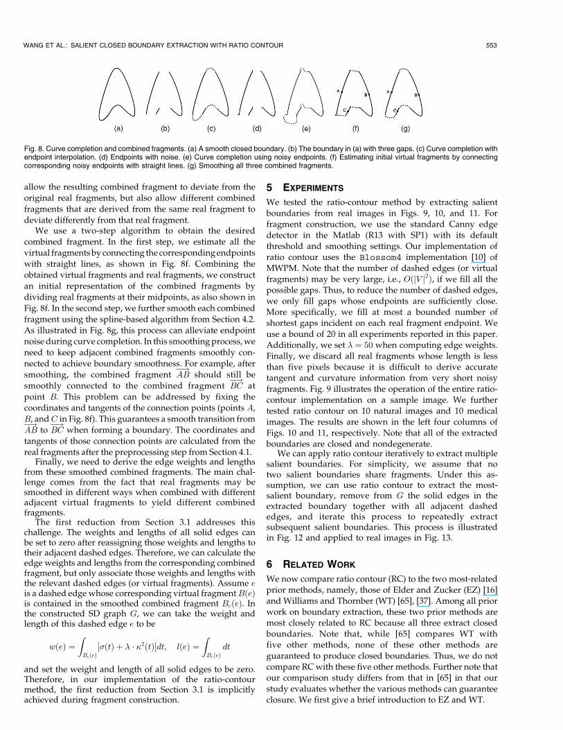
allow the resulting combined fragment to deviate from the

original real fragments, but also allow different combined

fragments that are derived from the same real fragment to

deviate differently from that real fragment.We use a two-step algorithm to obtain the desired

combined fragment. In the first step, we estimate all the

virtual fragmentsbyconnecting the correspondingendpoints

with straight lines, as shown in Fig. 8f. Combining the

obtained virtual fragments and real fragments, we construct

an initial representation of the combined fragments by

dividing real fragments at their midpoints, as also shown in

Fig. 8f. In the second step, we further smooth each combined

fragment using the spline-based algorithm from Section 4.2.

As illustrated in Fig. 8g, this process can alleviate endpoint

noise during curve completion. In this smoothingprocess,we

need to keep adjacent combined fragments smoothly con-

nected to achieve boundary smoothness. For example, after

smoothing, the combined fragment AB�!

should still be

smoothly connected to the combined fragment BC�!

at

point B. This problem can be addressed by fixing the

coordinates and tangents of the connection points (points A,

B, andC in Fig. 8f). This guarantees a smooth transition from

AB�!

to BC�!

when forming a boundary. The coordinates and

tangents of those connection points are calculated from the

real fragments after the preprocessing step from Section 4.1.Finally, we need to derive the edge weights and lengths

from these smoothed combined fragments. The main chal-lenge comes from the fact that real fragments may besmoothed in different ways when combined with differentadjacent virtual fragments to yield different combinedfragments.

The first reduction from Section 3.1 addresses thischallenge. The weights and lengths of all solid edges canbe set to zero after reassigning those weights and lengths totheir adjacent dashed edges. Therefore, we can calculate theedge weights and lengths from the corresponding combinedfragment, but only associate those weights and lengths withthe relevant dashed edges (or virtual fragments). Assume eis a dashed edge whose corresponding virtual fragmentBðeÞis contained in the smoothed combined fragment BcðeÞ. Inthe constructed SD graph G, we can take the weight andlength of this dashed edge e to be

wðeÞ ¼ZBcðeÞ½�ðtÞ þ � � �2ðtÞ�dt; lðeÞ ¼

ZBcðeÞ

dt

and set the weight and length of all solid edges to be zero.Therefore, in our implementation of the ratio-contourmethod, the first reduction from Section 3.1 is implicitlyachieved during fragment construction.

5 EXPERIMENTS

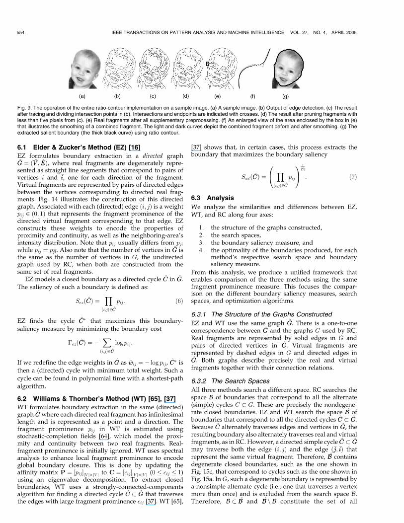
We tested the ratio-contour method by extracting salientboundaries from real images in Figs. 9, 10, and 11. For

fragment construction, we use the standard Canny edgedetector in the Matlab (R13 with SP1) with its defaultthreshold and smoothing settings. Our implementation ofratio contour uses the Blossom4 implementation [10] ofMWPM. Note that the number of dashed edges (or virtualfragments) may be very large, i.e., OðjV j2Þ, if we fill all thepossible gaps. Thus, to reduce the number of dashed edges,we only fill gaps whose endpoints are sufficiently close.More specifically, we fill at most a bounded number ofshortest gaps incident on each real fragment endpoint. We

use a bound of 20 in all experiments reported in this paper.Additionally, we set � ¼ 50 when computing edge weights.Finally, we discard all real fragments whose length is lessthan five pixels because it is difficult to derive accuratetangent and curvature information from very short noisyfragments. Fig. 9 illustrates the operation of the entire ratio-contour implementation on a sample image. We furthertested ratio contour on 10 natural images and 10 medicalimages. The results are shown in the left four columns of

Figs. 10 and 11, respectively. Note that all of the extractedboundaries are closed and nondegenerate.

We can apply ratio contour iteratively to extract multiplesalient boundaries. For simplicity, we assume that notwo salient boundaries share fragments. Under this as-sumption, we can use ratio contour to extract the most-salient boundary, remove from G the solid edges in theextracted boundary together with all adjacent dashededges, and iterate this process to repeatedly extractsubsequent salient boundaries. This process is illustratedin Fig. 12 and applied to real images in Fig. 13.

6 RELATED WORK

We now compare ratio contour (RC) to the two most-relatedprior methods, namely, those of Elder and Zucker (EZ) [16]and Williams and Thornber (WT) [65], [37]. Among all priorwork on boundary extraction, these two prior methods aremost closely related to RC because all three extract closedboundaries. Note that, while [65] compares WT withfive other methods, none of these other methods are

guaranteed to produce closed boundaries. Thus, we do notcompare RCwith these five other methods. Further note thatour comparison study differs from that in [65] in that ourstudy evaluates whether the various methods can guaranteeclosure. We first give a brief introduction to EZ and WT.

WANG ET AL.: SALIENT CLOSED BOUNDARY EXTRACTION WITH RATIO CONTOUR 553

Fig. 8. Curve completion and combined fragments. (a) A smooth closed boundary. (b) The boundary in (a) with three gaps. (c) Curve completion withendpoint interpolation. (d) Endpoints with noise. (e) Curve completion using noisy endpoints. (f) Estimating initial virtual fragments by connectingcorresponding noisy endpoints with straight lines. (g) Smoothing all three combined fragments.

6.1 Elder & Zucker’s Method (EZ) [16]

EZ formulates boundary extraction in a directed graphGG ¼ ðVV ; EEÞ, where real fragments are degenerately repre-sented as straight line segments that correspond to pairs ofvertices i and �ii, one for each direction of the fragment.Virtual fragments are represented by pairs of directed edgesbetween the vertices corresponding to directed real frag-ments. Fig. 14 illustrates the construction of this directedgraph. Associated with each (directed) edge ði; jÞ is a weightpij 2 ð0; 1Þ that represents the fragment prominence of thedirected virtual fragment corresponding to that edge. EZconstructs these weights to encode the properties ofproximity and continuity, as well as the neighboring-area’sintensity distribution. Note that pij usually differs from pjiwhile pij ¼ p�jj�ii. Also note that the number of vertices in GG isthe same as the number of vertices in G, the undirectedgraph used by RC, when both are constructed from thesame set of real fragments.

EZ models a closed boundary as a directed cycle CC in GG.

The saliency of such a boundary is defined as:

SezðCCÞ ¼Yði;jÞ2CC

pij: ð6Þ

EZ finds the cycle CC� that maximizes this boundary-

saliency measure by minimizing the boundary cost

�ezðCCÞ ¼ �Xði;jÞ2CC

log pij:

If we redefine the edge weights in GG as wwij ¼ � log pij, CC� is

then a (directed) cycle with minimum total weight. Such a

cycle can be found in polynomial time with a shortest-path

algorithm.

6.2 Williams & Thornber’s Method (WT) [65], [37]

WT formulates boundary extraction in the same (directed)graph GGwhere each directed real fragment has infinitesimallength and is represented as a point and a direction. Thefragment prominence pij in WT is estimated usingstochastic-completion fields [64], which model the proxi-mity and continuity between two real fragments. Real-fragment prominence is initially ignored. WT uses spectralanalysis to enhance local fragment prominence to encodeglobal boundary closure. This is done by updating theaffinity matrix P ¼ ½pij�jV j�jV j to C ¼ ½cij�jV j�jV j (0 � cij � 1)using an eigenvalue decomposition. To extract closedboundaries, WT uses a strongly-connected-componentsalgorithm for finding a directed cycle CC � GG that traversesthe edges with large fragment prominence cij [37]. WT [65],

[37] shows that, in certain cases, this process extracts theboundary that maximizes the boundary saliency

SwtðCCÞ ¼Yði;jÞ2CC

pij

0@

1A

1jCCj

: ð7Þ

6.3 Analysis

We analyze the similarities and differences between EZ,WT, and RC along four axes:

1. the structure of the graphs constructed,2. the search spaces,3. the boundary saliency measure, and4. the optimality of the boundaries produced, for each

method’s respective search space and boundarysaliency measure.

From this analysis, we produce a unified framework thatenables comparison of the three methods using the samefragment prominence measure. This focuses the compar-ison on the different boundary saliency measures, searchspaces, and optimization algorithms.

6.3.1 The Structure of the Graphs Constructed

EZ and WT use the same graph GG. There is a one-to-onecorrespondence between GG and the graphs G used by RC.Real fragments are represented by solid edges in G andpairs of directed vertices in GG. Virtual fragments arerepresented by dashed edges in G and directed edges inGG. Both graphs describe precisely the real and virtualfragments together with their connection relations.

6.3.2 The Search Spaces

All three methods search a different space. RC searches thespace B of boundaries that correspond to all the alternate(simple) cycles C � G. These are precisely the nondegene-rate closed boundaries. EZ and WT search the space BB ofboundaries that correspond to all the directed cycles CC � GG.Because CC alternately traverses edges and vertices in GG, theresulting boundary also alternately traverses real and virtualfragments, as in RC. However, a directed simple cycle CC � GGmay traverse both the edge ði; jÞ and the edge ð�jj; �iiÞ thatrepresent the same virtual fragment. Therefore, BB containsdegenerate closed boundaries, such as the one shown inFig. 15c, that correspond to cycles such as the one shown inFig. 15a. InG, such a degenerate boundary is represented bya nonsimple alternate cycle (i.e., one that traverses a vertexmore than once) and is excluded from the search space B.Therefore, B � BB and BB n B constitute the set of all

554 IEEE TRANSACTIONS ON PATTERN ANALYSIS AND MACHINE INTELLIGENCE, VOL. 27, NO. 4, APRIL 2005

Fig. 9. The operation of the entire ratio-contour implementation on a sample image. (a) A sample image. (b) Output of edge detection. (c) The resultafter tracing and dividing intersection points in (b). Intersections and endpoints are indicated with crosses. (d) The result after pruning fragments withless than five pixels from (c). (e) Real fragments after all supplementary preprocessing. (f) An enlarged view of the area enclosed by the box in (e)that illustrates the smoothing of a combined fragment. The light and dark curves depict the combined fragment before and after smoothing. (g) Theextracted salient boundary (the thick black curve) using ratio contour.

degenerate closed boundaries. While, in principle, EZ canproduce degenerate boundaries because it searches BB, itrarely produces degenerate boundaries, in practice, because,as analyzed later, EZ has a bias toward boundaries withfewer fragments.

WT employs the following local-search technique forfinding strongly connected components in an attempt toproduce nondegenerate closed boundaries: The techniqueselects an initial vertex k, expands the boundary byselecting the unvisited adjacent vertex j with maximumckj, and repeats this process on j until arriving back at k.This produces a cycle CCk. This same process is used toproduce a cycle CC�kk starting from �kk. A cycle CC0�kk ¼ f�iiji 2 CC�kkgis then constructed from CC�kk. Note that CCk, CC�kk, and CC0�kk allcorrespond to closed boundaries because they are necessa-rily cycles. However, they may be degenerate. WT attemptsto produce nondegenerate boundaries by taking CCk \ CC0�kk toderive a boundary. However, CCk \ CC0�kk might not be a cycleand, thus, might not correspond to a closed boundary. Forexample, consider the vertices k and �kk and the cycle CCk inFig. 15a. Since CCk contains both k and �kk, CCk and CC�kk can bethe same cycle. In this case, the subgraph CCk \ CC0�kkcorresponds to an open curve segment, as shown inFig. 15d. Such situations arise in the experiments presentedin the next section.

6.3.3 The Boundary Saliency MeasureAll three methods adopt a different boundary saliencymeasure. As seen by (6), EZ formulates boundary saliencyas the product of fragment prominence. As seen by (7), WTformulates boundary saliency as the geometric mean offragment prominence. As pointed out in [65], EZ’sboundary saliency decreases more quickly than WTs asthe number of fragments along the boundary increases.Therefore, EZ favors boundary with fewer fragments that,in many cases, results in short boundaries.

To compare the boundary saliency measures of WT andRC, we can redefine the edge weight wwij ¼ � log pij in GG torepresent fragment cost. Then, the cycle CC� that maximizesthe boundary saliency (7) is the same as the one thatminimizes the boundary cost

�wtðCCÞ ¼Pði;jÞ2CC wwij

jCCj:

This has the same form as the RC boundary cost (4) when

limited to the case where solid edges in G have zero weight

and length and dashed edges have unit length. While WT

and RC employ similar boundary saliency measures in this

limited case, they can still produce different results, even in

this limited case, because they search different spaces.

WANG ET AL.: SALIENT CLOSED BOUNDARY EXTRACTION WITH RATIO CONTOUR 555

Fig. 10. Boundary extraction on 10 natural images. Column 1: original image. Column 2: output of Canny edge detection. Column 3: real fragmentsconstructed by supplementary preprocessing. Column 4: the most-salient boundary extracted by RC on column 3. Column 5: real fragmentsconstructed by the unified framework. Columns 6 through 9: the most-salient boundaries detected by EZ, WT, (P-)RC, and C-RC on column 5.Columns 2 through 4 correspond to experiments discussed in Section 5. Columns 5 through 9 correspond to experiments discussed in Section 7.Image size is indicated under the images in column 1 and processing time in CPU seconds is indicated under the images in the remaining columns.See Section 7.5 for details on the measurement of processing time. Note that some closed boundaries have been cropped by the image perimeterwhen producing this figure.

6.3.4 The Optimality of the Boundaries Produced

Elder and Zucker [16] show that EZ is guaranteed to finda boundary that optimizes the boundary saliency measure�ez within the search space BB of closed boundarieswhether degenerate or nondegenerate. This paper showsthat RC is guaranteed to find a closed boundary thatoptimizes the boundary saliency measure �rc within thesearch space B of nondegenerate closed boundaries. Weknow of no proof that WT is guaranteed to find aboundary that optimizes the boundary saliency measure�wt within either BB or B.

6.3.5 Unified FrameworkThe three methods use different kinds of real fragments.In EZ, real fragments are line segments. In WT, realfragments are line segments with infinitesimal length. InRC, real fragments are quadratic splines. To facilitateexperimental comparison, we apply all three methods tothe kind of real fragments used by WT, namely, linesegments with infinitesimal length. The three methods usedifferent approaches to gap filling for constructing virtualfragments. To facilitate experimental comparison, weapply all three methods to virtual fragments constructed

using the stochastic-completion field method [64] of WTwith the parameters � ¼ 0:15, T ¼ 0:004, and � ¼ 5:0, assuggested in [64], [37].

The three methods use different fragment prominencemeasures. In EZ and WT, edge weights pij representfragment prominence, while, in RC, edge weights wð�Þrepresent fragment cost. Furthermore, EZ and WT onlyassociate prominence with virtual fragments, not realfragments, while RC associates costs with both. Finally, inWT, the number of virtual fragments along the boundary,i.e., jCCj, is used tomeasure the boundary length,while, in RC,boundary length is taken to be the total fragment length.

To facilitate experimental comparison, we apply allthree methods to the same prominence measure con-structed as follows: First, we take the weights pij used byEZ and WT to be related to the weights wð�Þ used by RCby the relation wði2; j1Þ ¼ � log pij, given that the undir-ected dashed edge ði2; j1Þ in G and the directed edge ði; jÞin GG correspond to the same virtual fragment, as shownin Fig. 14. Second, we take the length of all dashed edgesin G to be one and the weight and length of all solidedges in G to be zero. While this fragment prominence

556 IEEE TRANSACTIONS ON PATTERN ANALYSIS AND MACHINE INTELLIGENCE, VOL. 27, NO. 4, APRIL 2005

Fig. 11. Boundary extraction on 10 medical images. The columns depict the same information as in Fig. 10.

measure is a special case of the ones used in EZ and RC,it is compatible with all three algorithms.

7 COMPARISON STUDY

Unless otherwise noted, all the experiments reported in thissection use the unified framework of Section 6.3.

7.1 An Illustrative Example

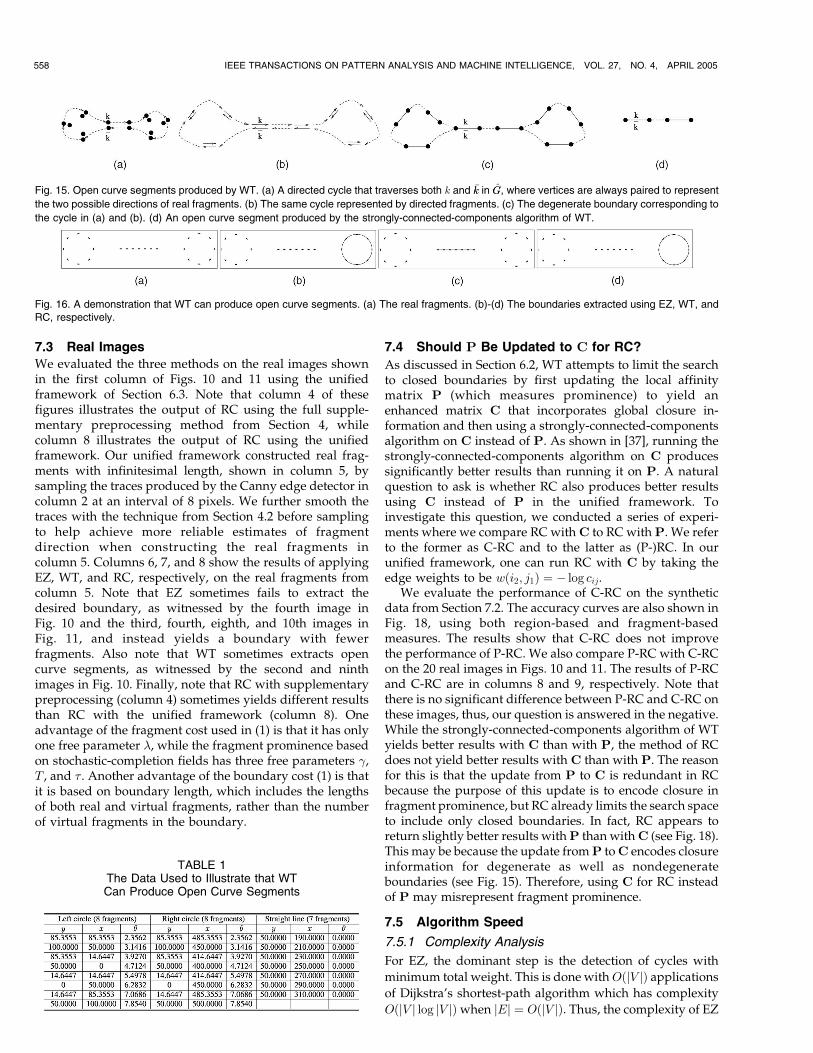
We construct a simple synthetic example to show that WTcan produce open curve segments. The real fragments inthis examples are shown in Fig. 16a. Sixteen real fragmentswere constructed by sampling two circles of radius 100 andseven addition real fragments were constructed by sam-pling a straight line segment placed between thesetwo circles. The exact information needed to reconstructthis example is given in Table 1. Figs. 16b, 16c, and 16dshow the most-salient boundaries extracted using EZ, WT,and RC, respectively. This confirms that WT can produceopen curve segments, as discussed in Section 6.3.

7.2 Synthetic Data

As in [65], we constructed a set of synthetic data toquantitatively evaluate the performance of EZ, WT, andRC. In this data, the input real fragments containtwo superimposed patterns: a foreground pattern and abackground pattern. The foreground pattern is selected fromthe nine objects shown in Fig. 17, where the object boundaryis uniformly sampled to construct the real fragments for theforeground pattern. The first five fruit patterns shown inFig. 17 were used in [65]. As in [65], the real fragments for thebackground pattern is derived from nine texture images:bark, fabric, sand, terrain, wood, brick, leaves, stone, andwater, by uniformly sampling their edge-detector outputs.In this experiment, we sample each foreground-objectboundary with seven different sampling rates to constructa set of synthetic data with varied signal to noise ratio (SNR).Here, we define the SNR as the ratio between the number ofreal fragments from the foreground pattern and the numberof real fragments from the background pattern. This way, we

have a total of 9� 9� 7 ¼ 567 synthetic data samples for ourexperiments by superimposing a foreground pattern with abackground pattern.

We applied both EZ, WT, and RC to extract the most-salient boundaries from all these 567 data samples. Theaccuracy is then evaluated by comparing the extractedsalient boundaries and the underlying foreground objectboundaries. We evaluate the accuracy using twomeasures: aregion-based measure and a fragment-based measure. Theregion-based accuracy measure is defined as the relativeregion coincidence,

jR1 \R2jjR1 [R2j

;

where R1 is the region of the foreground object, R2 is theregion enclosed by the detected salient boundary, and jRjdenotes the area ofR. The fragment-based accuracy measureis defined as the percentage of real fragments for theforeground pattern that are included in the detected salientboundary. Figs. 18a and18c showtheperformance of EZ,WT,andRC on all 567 synthetic data samples using the above twomeasures.Note that the accuracy at each SNR is calculated bytaking the average accuracy on 9� 9 ¼ 81 data samples withthis SNR. In this experiment, WT produces open curvesegments in 170 data samples out of the 567 data samples andits performance is degraded greatly by these 170 samples.Figs. 18band18dshowtheperformanceofEZ,WT,andRConthe remaining 397 data samples where all three methodsproduce closed boundaries. We see that WT has no betterperformance than RC, even if we only count these 397 datasamples. Four examples of these experiments are shown inFig. 19, where WT produces open curve segments in thesecond and third images.

WANG ET AL.: SALIENT CLOSED BOUNDARY EXTRACTION WITH RATIO CONTOUR 557

Fig. 12. Extracting multiple salient boundaries. (a) The original SD graphfrom Fig. 1e. (b) The new SD graph after extracting the most-salientboundary corresponding to the cycle (thick lines) shown in (a). Note thatfrom (a) to (b), we remove not only all solid and dashed edges in thecycle corresponding to the most-salient boundary, but also all thedashed edges adjacent to the removed solid edges. A second iterationof ratio contour on this new SD graph yields the second most-salientboundary, shown in thick lines in (b).

Fig. 14. The directed graph GG used in EZ and WT. (a) Initial real/virtual fragments and the SD graph G, (b) directed real/virtual fragments, and (c) theresulting directed graph GG analogous to (a). This figure is adapted from Fig. 3 from [65].

Fig. 13. Extracting multiple salient boundaries from seven real images

with iterative ratio contour. Each row depicts an original image, the

edge-detector output, and the sequence of boundaries extracted for that

image. The images in the last two rows come from [37].

7.3 Real Images

We evaluated the three methods on the real images shownin the first column of Figs. 10 and 11 using the unifiedframework of Section 6.3. Note that column 4 of thesefigures illustrates the output of RC using the full supple-mentary preprocessing method from Section 4, whilecolumn 8 illustrates the output of RC using the unifiedframework. Our unified framework constructed real frag-ments with infinitesimal length, shown in column 5, bysampling the traces produced by the Canny edge detector incolumn 2 at an interval of 8 pixels. We further smooth thetraces with the technique from Section 4.2 before samplingto help achieve more reliable estimates of fragmentdirection when constructing the real fragments incolumn 5. Columns 6, 7, and 8 show the results of applyingEZ, WT, and RC, respectively, on the real fragments fromcolumn 5. Note that EZ sometimes fails to extract thedesired boundary, as witnessed by the fourth image inFig. 10 and the third, fourth, eighth, and 10th images inFig. 11, and instead yields a boundary with fewerfragments. Also note that WT sometimes extracts opencurve segments, as witnessed by the second and ninthimages in Fig. 10. Finally, note that RC with supplementarypreprocessing (column 4) sometimes yields different resultsthan RC with the unified framework (column 8). Oneadvantage of the fragment cost used in (1) is that it has onlyone free parameter �, while the fragment prominence basedon stochastic-completion fields has three free parameters �,T , and � . Another advantage of the boundary cost (1) is thatit is based on boundary length, which includes the lengthsof both real and virtual fragments, rather than the numberof virtual fragments in the boundary.

7.4 Should P Be Updated to C for RC?

As discussed in Section 6.2, WT attempts to limit the searchto closed boundaries by first updating the local affinitymatrix P (which measures prominence) to yield anenhanced matrix C that incorporates global closure in-formation and then using a strongly-connected-componentsalgorithm on C instead of P. As shown in [37], running thestrongly-connected-components algorithm on C producessignificantly better results than running it on P. A naturalquestion to ask is whether RC also produces better resultsusing C instead of P in the unified framework. Toinvestigate this question, we conducted a series of experi-ments where we compare RC withC to RC with P. We referto the former as C-RC and to the latter as (P-)RC. In ourunified framework, one can run RC with C by taking theedge weights to be wði2; j1Þ ¼ � log cij.

We evaluate the performance of C-RC on the syntheticdata from Section 7.2. The accuracy curves are also shown inFig. 18, using both region-based and fragment-basedmeasures. The results show that C-RC does not improvethe performance of P-RC. We also compare P-RC with C-RCon the 20 real images in Figs. 10 and 11. The results of P-RCand C-RC are in columns 8 and 9, respectively. Note thatthere is no significant difference between P-RC and C-RC onthese images, thus, our question is answered in the negative.While the strongly-connected-components algorithm of WTyields better results with C than with P, the method of RCdoes not yield better results with C than with P. The reasonfor this is that the update from P to C is redundant in RCbecause the purpose of this update is to encode closure infragment prominence, but RC already limits the search spaceto include only closed boundaries. In fact, RC appears toreturn slightly better results withP than withC (see Fig. 18).This may be because the update fromP toC encodes closureinformation for degenerate as well as nondegenerateboundaries (see Fig. 15). Therefore, using C for RC insteadof P may misrepresent fragment prominence.

7.5 Algorithm Speed

7.5.1 Complexity Analysis

For EZ, the dominant step is the detection of cycles with

minimum total weight. This is done withOðjV jÞ applicationsof Dijkstra’s shortest-path algorithm which has complexity

OðjV j log jV jÞwhen jEj ¼ OðjV jÞ. Thus, the complexity of EZ

558 IEEE TRANSACTIONS ON PATTERN ANALYSIS AND MACHINE INTELLIGENCE, VOL. 27, NO. 4, APRIL 2005

Fig. 15. Open curve segments produced by WT. (a) A directed cycle that traverses both k and �kk in GG, where vertices are always paired to represent

the two possible directions of real fragments. (b) The same cycle represented by directed fragments. (c) The degenerate boundary corresponding to

the cycle in (a) and (b). (d) An open curve segment produced by the strongly-connected-components algorithm of WT.

Fig. 16. A demonstration that WT can produce open curve segments. (a) The real fragments. (b)-(d) The boundaries extracted using EZ, WT, andRC, respectively.

TABLE 1The Data Used to Illustrate that WTCan Produce Open Curve Segments

is OðjV j2 log jV jÞ. For WT, the dominant step is to compute

the principle eigenvector of P, a reversal matrix whose size

is jVV j � jVV j. If jEEj ¼ OðjVV jÞ, then P is sparse and has OðjVV jÞnonzero entries. Note that jV j ¼ jVV j. The principle eigen-

vector of an arbitrary dense matrix of size jV j � jV j can be

computed in OðjV j2Þ time. We do not know if the fact that P

is sparse or is a reversal matrix can reduce this time

complexity. For RC, the dominant step is the third reduction

from Section 3, namely, MWPM. Gabow [17] shows that the

time-complexity for finding an MWPM in an integer-

weighted graph G ¼ ðV ;EÞ is OðjV j34jEj logwmaxÞ, where

wmax is the maximum edge weight in the graph. In practice,

since each vertex is only connected to a bounded number of

vertices, jEj ¼ OðjV jÞ. Thus, the complexity of RC is OðjV j74Þ.

7.5.2 Running Times

Figs. 10 and 11 indicate the running times, in CPU seconds,of various steps of the different methods. Column 2indicates the time to perform edge detection. Column 3indicates the time to perform supplementary preprocessingto construct the graph G. Column 4 indicates the runningtime of RC after constructing G. Column 5 indicates thetime to construct GG. Columns 6 through 9 indicate therunning times of EZ, WT, P-RC, and C-RC after construct-ing GG. All experiments were conducted on a Dell PrecisionWorkstation equipped with a 3.06GHz Intel Xeon Processorwith a 512K L2 Cache.

8 CONCLUSION

We have presented ratio contour, a novel method forextracting salient closed boundaries from noisy images.Starting with a set of boundary fragments that are detectedin images using an edge detector, ratio contour is able toidentify a subset of those fragments and connect themsequentially into a closed boundarywith the largest saliency.

Boundary saliency encodes the Gestalt laws of closure,proximity, and continuity. Our paper makes several con-tributions. First, it formulates a new boundary-saliencymeasure in terms of a ratio that is normalized relative toboundary length. This effectively avoids the possible biastoward short boundaries. Second, it presents a novelpolynomial-time algorithm for finding the most-salientclosed boundary with the saliency measure. Third, ourmethod finds only closed nondegenerate boundaries byprecisely constraining the search space to include only suchdesired boundaries. Fourth, it presents a novel collection ofpreprocessing methods to reduce the effects of noise onboundary detection. Finally, it constructs a unified frame-work for comparing ratio contour with two closely relatedprevious methods, EZ and WT, and conducts such acomparison.

WANG ET AL.: SALIENT CLOSED BOUNDARY EXTRACTION WITH RATIO CONTOUR 559

Fig. 17. The nine foreground patterns used for constructing synthetic data. From the left to the right are the patterns of a lemon, a pear, a peach, an

onion, an apple, a knife, a spoon, a handsaw, and an oil can, respectively.

Fig. 18. Accuracy in extracting the foreground patterns out of background patterns. (a) Region-based accuracy computed on all 567 data samples.

(b) Region-based accuracy computed on the 397 data samples where WT produces closed boundaries. (c) Fragment-based accuracy computed on

all 567 data samples. (d) Fragment-based accuracy computed on the 397 data samples where WT produces closed boundaries. The curve for C-RC

and the notation P-RC will be explained in Section 7.4.

Fig. 19. Extracting salient boundaries on four synthetic data samples.From the leftmost column to the rightmost column are the real fragmentsand the boundaries extracted using EZ, WT, (P-)RC, and C-RC,respectively. The meaning of (P-)RC and C-RC will be explained inSection 7.4. From the top row to the bottom row are the superimposedpatterns of onion and terrain, spoon and stone, knife and leaves, andpeach and fabric, respectively.

Our comparison yields the following findings:

1. EZ shows a bias toward boundaries with fewerfragments, whileWT and RCdo not show such a bias.

2. WT may produce open curve segments, while RC isguaranteed to produce closed boundaries.

3. The space searched by EZ and WT includesdegenerate boundaries, while the space searchedby RC does not.

4. Adding the fragment-prominence update methodused by WT to RC does not appreciably improveperformance.

5. Experimental evaluation on natural and medicalimages shows that RC produces results that are asgood as or better than EZ and WT.

We hope that the techniques underlying ratio contour will

lead to future advances in boundary extraction.

ACKNOWLEDGMENTS

The authors would like to thank David Jacobs for important

comments on an earlier draft of this paper. This work was

funded, in part, by US National Science Foundation grants

0312861EIA and 0329156IIS. Some preliminary results from

this paper were reported in [60] and [62].

REFERENCES

[1] R.K. Ahuja, T.L. Magnanti, and J.B. Orlin, Network Flows: Theory,Algorithms, & Applications. Prentice Hall, 1993.

[2] T. Alter and R. Basri, “Extracting Salient Contours from Images:An Analysis of the Saliency Network,” Proc. IEEE Conf. ComputerVision and Pattern Recognition, pp. 13-20, 1996.

[3] A.A. Amini, T.E. Weymouth, and R.C. Jain, “Using DynamicProgramming for Solving Variational Problems in Vision,” IEEETrans. Pattern Analysis and Machine Intelligence, vol. 12, no. 9,pp. 855-867, 1990.

[4] A. Amir and M. Lindenbaum, “A Generic Grouping Algorithmand Its Quantitative Analysis,” IEEE Trans. Pattern Analysis andMachine Intelligence, vol. 20, no. 2, pp. 168-185, Feb. 1998.

[5] A. Barbu and S.C. Zhu, “Graph Partition by Swendsen-WangCuts,” Proc. Int’l Conf. Computer Vision, 2003.

[6] K. Bowyer, C. Kranenburg, and S. Dougherty, “Edge DetectorEvaluation Using Empirical ROC Curves,” Computer Vision andImage Understanding, vol. 84, no. 10, pp. 77-103, 2001.

[7] J. Canny, “A Computational Approach to Edge Detection,” IEEETrans. Pattern Analysis and Machine Intelligence, vol. 8, no. 6,pp. 679-698, 1986.

[8] V. Casselles, F. Catte, T. Coll, and F. Dibos, “AGeometricModel forActive Contours,” Numerische Mathematik, vol. 66, no. 1, pp. 1-31,1993.

[9] L.D. Cohen and I. Cohen, “A Finite Element Method Applied toNew Active Contour Models and 3D Reconstruction from CrossSections,” Proc. Int’l Conf. Computer Vision, pp. 587-591, 1990.

[10] W. Cook and A. Rohe, “Computing Minimum-Weight PerfectMatchings,” http://www.or.unibonn.de/home/rohe/matching.html, Aug. 1998.

[11] T.F. Cootes, C.J. Taylor, D.H. Cooper, and J. Graham, “ActiveShape Models—Their Training and Application,” Computer Visionand Image Understanding, vol. 61, no. 1, pp. 38-59, 1995.

[12] T.H. Cormen, C.E. Leiserson, and R.L. Rivest, Introduction toAlgorithms. Cambridge: MIT Press and New York: McGraw Hill,1990.

[13] I. Cox, S.B. Rao, and Y. Zhong, “Ratio Regions: A Technique forImage Segmentation,” Proc. Int’l Conf. Pattern Recognition, pp. 557-564, 1996.

[14] E. Dijkstra, “Note on Two Problems in Connection with Graphs,”Numerische Mathematik, vol. 1, pp. 269-271, 1959.

[15] J. Edmonds, “Path, Trees, and Flowers,” Canadian J. Math., vol. 17,pp. 449-467, 1965.

[16] J. Elder and S. Zucker, “Computing Contour Closure,” Proc.European Conf. Computer Vision, pp. 399-412, 1996.

[17] H.N. Gabow, “A Scaling Algorithm for Weighted Matching onGeneral Graphs,” Proc. 26th Ann. Symp. Foundations of ComputerScience, pp. 90-100, 1985.

[18] M. Galun, E. Sharon, R. Basri, and A. Brandt, “TextureSegmentation by Multiscale Aggregation of Filter Responses andShape Elements,” Proc. Int’l Conf. Computer Vision, 2003.

[19] Y. Gdalyahu, D. Weinshall, and M. Werman, “Stochastic ImageSegmentation by Typical Cuts,” Proc. IEEE Conf. Computer Visionand Pattern Recognition, pp. 596-601, 1999.

[20] S. Geman and D. Geman, “Stochastic Relaxation, Gibbs Distribu-tion, and the Bayesian Restoration of Images,” IEEE Trans. PatternAnalysis and Machine Intelligence, vol. 6, no. 6, pp. 721-741, 1984.

[21] G. Guy and G. Medioni, “Inferring Global Perceptual Contoursfrom Local Features,” Int’l J. Computer Vision, vol. 20, no. 1, pp. 113-133, 1996.

[22] X. Han, C. Xu, and J.L. Prince, “A Topology PreservingDeformable Model Using Level Set,” Proc. IEEE Conf. ComputerVision and Pattern Recognition, vol. 2, pp. 765-770, 2001.

[23] P. Hart, N. Nilsson, and B. Raphael, “A Formal Basis for theHeuristic Determination of Minimum-Cost Path,” IEEE Trans.Systems, Man, and Cybernetics, vol. 4, pp. 100-107, 1968.

[24] M.D. Heath, S. Sarkar, T. Sanocki, and K.W. Bowyer, “A RobustVisual Method for Assessing the Relative Performance of Edge-Detection Algorithms,” IEEE Trans. Pattern Analysis and MachineIntelligence, vol. 19, no. 12, pp. 1338-1359, Dec. 1997.

[25] L. Herault and R. Horaud, “Figure-Ground Discrimination: ACombinatorial Optimization Approach,” IEEE Trans. PatternAnalysis and Machine Intelligence, vol. 15, pp. 899-914, 1993.

[26] L.A. Iverson and S.W. Zuker, “Logic/Linear Operators for ImageCurves,” IEEE Trans. Pattern Analysis and Machine Intelligence,vol. 17, no. 10, pp. 982-996, Oct. 1995.

[27] D. Jacobs, “Robust and Efficient Detection of Convex Groups,”IEEE Trans. Pattern Analysis and Machine Intelligence, vol. 18, no. 1,pp. 23-37, Jan. 1996.

[28] A.K. Jain, Y. Zhong, and S. Lakshmanan, “Object Matching UsingDeformable Templates,” IEEE Trans. Pattern Analysis and MachineIntelligence, vol. 18, no. 3, pp. 267-278, Mar. 1996.

[29] I.H. Jermyn and H. Ishikawa, “Globally Optimal Regions andBoundaries as Minimum Ratio Cycles,” IEEE Trans. PatternAnalysis and Machine Intelligence, vol. 23, no. 10, pp. 1075-1088,Oct. 2001.

[30] M. Kass, A. Witkin, and D. Terzopoulos, “Snakes: Active ContourModels,” Int’l J. Computer Vision, vol. 1, no. 4, pp. 321-331, 1988.

[31] B.B. Kimia, I. Frankel, and A.-M. Popescu, “Euler Spiral for ShapeCompletion,” Int’l J. Computer Vision, vol. 54, pp. 157-180, 2003.

[32] S. Konishi, A.L. Yuille, J.M. Coughlan, and S.C. Zhu, “StatisticalEdge Detection: Learning and Evaluating Edge Cues,” IEEE Trans.Pattern Analysis and Machine Intelligence, vol. 25, no. 1, pp. 57-74,Jan. 2003.

[33] I. Kovacs and B. Julesz, “A Closed Curve is Much More than anIncomplete One: Effect of Closure in Figure-Ground Segmenta-tion,” Proc. Nat’l Academy of Science USA, vol. 90, pp. 7495-7497,1993.

[34] T. Kubota, “Contextual and Non-Combinatorial Approach toFeature Extraction,” Proc. Int’l Workshop Energy MinimizationMethods in Computer Vision and Pattern Recognition, 2003.

[35] T.-S. Lee, D. Mumford, and A. Yuille, “Texture Segmentation byMinimizing Vector-Valued Energy Functionals: The Coupled-Membrane Model,” Proc. European Conf. Computer Vision, pp. 165-183, 1992.

[36] M.E. Leventon, E.L. Grimson, and O. Faugeras, “Statistical ShapeInfluence in Geodesic Active Contours,” Proc. IEEE Conf. ComputerVision and Pattern Recognition, pp. 316-323, 2000.

[37] S. Mahamud, L.R. Williams, K.K. Thornber, and K. Xu, “Segmen-tation of Multiple Salient Closed Contours from Real Images,”IEEE Trans. Pattern Analysis and Machine Intelligence, vol. 25, no. 4,pp. 433-444, Apr. 2003.

[38] D.Mumford, “Bayesian Rationale for theVariational Formulation,”Geometry-Driven Diffusion in Computer Vision, B.M.H. Romeny, ed.,pp. 135-143, Kluwer, 1994.

[39] M. Nitzberg, D. Mumford, and T. Shiota, “Filtering, Segmentationand Depth,” Lecture Notes in Computer Science, vol. 662, New York:Springer-Verlag, 1993.

[40] P. Perona, “A Factorization Approach to Grouping,” Proc.European Conf. Computer Vision, pp. 655-670, 1998.

560 IEEE TRANSACTIONS ON PATTERN ANALYSIS AND MACHINE INTELLIGENCE, VOL. 27, NO. 4, APRIL 2005

[41] J.M. Prewitt, “Object Enhancement and Extraction,” PictureProcessing and Psychopictorics, B. Lipkin and A. Rosenfeld, eds.,pp. 75-149, New York: Academic Press, 1970.

[42] S. Raman, S. Sarkar, and K. Boyer, “Hypothesizing Structures inEdge-Focused Cerebral Magnetic Resonance Images Using Graph-Theoretic Cycle Enumeration,” Computer Vision, Graphics, andImage Processing, vol. 57, no. 1, pp. 81-98, 1993.

[43] K.R. Rao and J. Ben-Arie, “Optimal Edge Detection UsingExpansionMatching and Restoration,” IEEE Trans. Pattern Analysisand Machine Intelligence, vol. 16, no. 12, pp. 1169-1182, Dec. 1994.

[44] X. Ren and J. Malik, “A Probabilistic Multi-Scale Model forContour Completion Based on Image Statistics,” Proc. EuropeanConf. Computer Vision, vol. 1, pp. 312-327, 2002.

[45] L.G. Roberts, “Machine Perception of Three-Dimensional Solids,”Optical and Electro-Optical Information Processing, J.T. Tippett, ed.,pp. 159-197, Cambridge, Mass.: Massachusetts Inst. of TechnologyPress, 1965.

[46] B.M.H. Romeny, Geometry-Driven Diffusion in Computer Vision.Dordrecht & Boston: Kluwer Academic Publishers, 1994.

[47] D. Rueckert and P. Burger, “Geometrically Deformable Templatesfor Shape-Based Segmentation and Tracking in Cardiac MRImage,” Proc. Int’l Workshop Energy Minimization Methods inComputer Vision and Pattern Recognition, pp. 83-98, 1997.

[48] S. Sarkar andK. Boyer, “QuantitativeMeasures of Change Based onFeature Organization: Eigenvalues and Eigenvectors,” Proc. IEEEConf. Computer Vision and Pattern Recognition, pp. 478-483, 1996.

[49] S. Sarkar and P. Soundararajan, “Supervised Learning of LargePerceptual Organization: Graph Spectral Partitioning and Learn-ing Automata,” IEEE Trans. Pattern Analysis and Machine Intelli-gence, vol. 22, no. 5, pp. 504-525, May 2000.

[50] E. Sharon, A. Brandt, and R. Basri, “Completion Energies andScale,” IEEE Trans. Pattern Analysis and Machine Intelligence, vol. 22,no. 10, pp. 1117-1131, Oct. 2000.

[51] E. Sharon, A. Brandt, and R. Basri, “Fast Multiscale ImageSegmentation,” Proc. IEEE Conf. Computer Vision and PatternRecognition, vol. 1, pp. 70-77, 2000.

[52] E. Sharon, A. Brandt, and R. Basri, “Segmentation and BoundaryDetection Using Multiscale Intensity Measurements,” Proc. IEEEConf. Computer Vision and Pattern Recognition, vol. 1, pp. 469-476,2001.

[53] A. Shashua and S. Ullman, “Structural Saliency: The Detection ofGlobally Salient Structures Using a Locally Connected Network,”Proc. Int’l Conf. Computer Vision, pp. 321-327, 1988.

[54] J. Shi and J. Malik, “Normalized Cuts and Image Segmentation,”IEEE Trans. Pattern Analysis and Machine Intelligence, vol. 22, no. 8,pp. 888-905, Aug. 2000.

[55] I.E. Sobel, “Camera Models and Machine Perception,” PhDdissertation, Stanford Univ., Stanford, Calif., 1970.

[56] P. Soundararajan and S. Sarkar, “An In-Depth Study of GraphPartitioning Measures for Perceptual Organization,” IEEE Trans.Pattern Analysis and Machine Intelligence, vol. 25, no. 6, pp. 642-660,June 2003.

[57] L.H. Staib and J.S. Ducan, “Boundary Finding with ParametricallyDeformable Models,” IEEE Trans. Pattern Analysis and MachineIntelligence, vol. 17, no. 11, pp. 1061-1075, Nov. 1992.

[58] K.K. Thornber and L.R. Williams, “Analytic Solution of StochasticCompletion Fields,”Biological Cybernetics, vol. 75, pp. 141-151, 1996.

[59] O. Veksler, “Image Segmentation by Nested Cuts,” Proc. IEEEConf. Computer Vision and Pattern Recognition, pp. 339-344, 2000.

[60] S. Wang, T. Kubota, and J.M. Siskind, “Salient Boundary DetectionUsing Ratio Contour,” Proc. Neural Information Processing SystemsConf., pp. 1571-1578, 2003.

[61] S. Wang and J.M. Siskind, “Image Segmentation with Ratio Cut,”IEEE Trans. Pattern Analysis and Machine Intelligence, vol. 25, no. 6,pp. 675-690, June 2003.

[62] S. Wang, J. Wang, and T. Kubota, “From Fragments to SalientClosed Boundaries: An In-Depth Study,” Proc. IEEE Conf.Computer Vision and Pattern Recognition, vol. I, pp. 291-298, 2004.

[63] D.J. Williams and M. Shah, “A Fast Algorithm for ActiveContours,” Proc. Int’l Conf. Computer Vision, pp. 592-595, 1990.

[64] L. Williams and D. Jacobs, “Stochastic Completion Fields: ANeural Model of Illusory Contour Shape and Salience,” NeuralComputation, vol. 9, pp. 849-870, 1997.

[65] L. Williams and K.K. Thornber, “A Comparison Measures forDetecting Natural Shapes in Cluttered Background,” Int’l J.Computer Vision, vol. 34, nos. 2/3, pp. 81-96, 2000.

[66] Z. Wu and R. Leahy, “An Optimal Graph Theoretic Approach toData Clustering: Theory and Its Application to Image Segmenta-tion,” IEEE Trans. Pattern Analysis and Machine Intelligence, vol. 15,no. 11, pp. 1101-1113, Nov. 1993.

[67] C. Xu and J.L. Prince, “Snakes, Shapes, and Gradient VectorFlow,” IEEE Trans. Image Processing, vol. 7, no. 3, pp. 359-369, 1998.

[68] S.C. Zhu and A. Yuille, “Region Competition: Unifying Snakes,Region Growing, and Bayes/MDL for Multi-Band Image Seg-mentation,” IEEE Trans. Pattern Analysis and Machine Intelligence,vol. 18, no. 9, pp. 884-900, Sept. 1996.

Song Wang received the PhD degree inelectrical and computer engineering from theUniversity of Illinois at Urbana-Champaign in2002. From 1998 to 2002, he also worked as aresearch assistant in the Image Formation andProcessing Group of the Beckman Institute,University of Illinois at Urbana-Champaign.Since August 2002, he has been an assistantprofessor in the Department of ComputerScience and Engineering at the University of

South Carolina. His research interests include computer vision, medicalimage processing, and machine learning. He is a member of the IEEEand the IEEE Computer Society.

Toshiro Kubota received the BS degree fromKeio University, Japan, in 1988, and the MS andPhD degrees from the Georgia Institute ofTechnology, Atlanta, in 1989 and 1995, respec-tively. From 1996 until 2004, he was at theUniversity of South Carolina, Columbia. He wasan assistant professor from 2000 to 2004 anddirected the Intelligent Systems Laboratory from1999 to 2004. In 2004, he started a consultingbusiness applying image processing and com-

puter vision techniques to real-world problems. His research interestsinclude computational vision, low-level vision, and neural networks. Heis a member of the ACM and the IEEE.

Jeffrey Mark Siskind received the BA degree incomputer science from the Technion, IsraelInstitute of Technology, in 1979, the SM degreein computer science from MIT in 1989, and thePhD degree in computer science from MIT in1992. He did a postdoctoral fellowship at theUniversity of Pennsylvania Institute for Researchin Cognitive Science from 1992 to 1993. He wasan assistant professor at the University ofToronto in the Department of Computer Science

from 1993 to 1995, a senior lecturer in the Technion Department ofElectrical Engineering in 1996, a visiting assistant professor at theUniversity of Vermont Department of Computer Science and ElectricalEngineering from 1996 to 1997, and a research scientist at NECResearch Institute, Inc. from 1997 to 2001. He joined the PurdueUniversity School of Electrical and Computer Engineering in 2002,where he is currently an associate professor. His research interestsinclude machine vision, artificial intelligence, cognitive science, compu-tational linguistics, child language acquisition, and programminglanguages and compilers. He is a member of the IEEE and the IEEEComputer Society.

Jun Wang received the bachelor’s degree fromShanghai JiaoTong University (SJTU) in July1998 and the master’s degree from the Depart-ment of Automation at Tsinghua University in2003. He was a graduate student in theDepartment of Computer Science and Engineer-ing, University of South Carolina, from August2003 to May 2004. His research interest iscomputer vision.

. For more information on this or any other computing topic,please visit our Digital Library at www.computer.org/publications/dlib.

WANG ET AL.: SALIENT CLOSED BOUNDARY EXTRACTION WITH RATIO CONTOUR 561