^s THE BEHAVIOUR OF ANNULAR FOOTINGS ON SAND

^s

THE BEHAVIOUR OF ANNULAR FOOTINGS ON SAND

ABSTRACT

Thesis submitted for the award of the Degree of

Bottor of $Ijilo£(opt)j> IN

CIVIL ENGINEERING (Soil Mechanics & Foundation Engineering)

by

SYED SALAHUDDIN SHAH

DEPARTMENT OF CIVIL ENGINEERING Z. H. COLLEGE OF ENGINEERING & TECHNOLOGY

ALIGARH MUSLIM UNIVERSITY ALIGARH (INDIA)

1994


ABSTR/iCT

The bearing capacity of a footiBg-soU Fysteo i*afi tc satisfy the

shear aod settlemeDt criter' for disigniag a fou. da>.loD. A ireat deal

of vork has aJready been done for predicting the bearing capa'l y of a

foujidatioD on sandy soil for conventional shape of footings like square,

circular and strip footings. However owing to scarcity of field and

laboratory tests data for annuler footing on sand, it has not been

possible to give a definite formula for the bearing capacity and

settleuent behaviour of these footings. The laboratory tests conducted

by Haroon et al., (1980), Saha (1978) ar' Kaxroo (1985) have provided

qualitative iDformation regarding the behaviour of ainular footings on

sand. Since sraaJJ scale model test results are looked upon with

suspicion, the author investigated the problem using large size annular

footing with different annularity ratios. The rigid an ular model

footing of external diameter 200 mm, 300 mm and 400 mo with five

different ratios of Internal to external diameter, h/d ° C O , 0.3, 0.4,

0.5, 0.6 and 0,7 have been used.

The vork includes model studies based on dimensional analysis. An

equation for the ultimate bearing capacity of a.ujuiar footing

introducing shape factor In the original Trezahl's equation has been

presented in this study.

The prediction of the settlement of annular foodng is highly

complicated due to the effect of annularity. In order to estimate the

setUement, the stress analysis below the annular footing is necessary.

(ii)

Closed iorm solution for the stress belov the annular footing is given

bv Egorov, (1965). Using the chart proposed by Egorov (1977), isobars

have been dravn for different annularlty ratios by the author, and the

same has been compared vith the solid circular footings. The stresses

have also been experimentally measured at different depths by the use of

pressure cells under the footings. The theoretical values of stresses

have also been worked out by softvaie progranuDe and data are given in

labular foriu.

The above concept can be used to estimate the elastic as veil as

iong term consolidation settlement of soil layers influenced by annular

footings. To the author's knowledge, there is no formula to predict the

settlement of annular prototype footing using plate-load test. It was

therefore felt necessary to find a formula similar to one suggested by

Terzaghi, in order to predict the settlement of prototype foundation

Dased on small size plate-load test. A non-dimensional settlement

eHiciency factor has been introduced by the author to predict the

sfetileoent of annular footing by using a circular plate-load test. The

settleaent as a function of annularity has been determined empirically

by using test data. The results have been compared with the Terzaghi

approach for predicting the settlement of solid circular footings. It

has been observed that the effect of size for annular foundation for the

same h/d ratios is similar to one suggested by Terzaghi'.


Thesis submitted for the award of the Degree of

©octor of ^bilogopfjp IN

CIVIL ENGINEERING (Soti Mechanics & Foundation Engiiieering)

by

SYED SALAHUDDIN SHAH

DEPARTMENT OF CIVIL ENGINEERING Z. H. COLLEGE OF ENGINEERING & TECHNOLOGY

ALIGARH MUSLIM UNIVERSITY ALIGARH (INDIA)

1994

T4241

r42^4 l

JU?^ 1334

^ c ^ '

C E R T I F I C A T E

Th-U, -ii to ctn.ti{iy that thz pKzânt the^li zntitizd 'THE

BEHAVIOUR Of KUmiMi. TOOTJUGS ON SAM)' bzing 6appUaatzd by UK. SVEV

SALAHUWW SHAH, {ô^ the, amid o{, VzQuaz oi VoctoK oi Phltoioph(f in thz

¥ acuity o(^ Engine-Zfiing, -Li a izcoid 0(J bonafîda KZiaafich uioik caiiizd

ovzK by him on thz a{ôKti,aid topic a6.6igmd to him by thz Committze {ÔK

Advanced Studizi and RzAzaich in iti mzzting hzid on 22.4.19S1.

KligaKh ( VK. Alixml Qadan. ) Vatzd: DfK ^ ^ ^ - )^^4 ?ioiU60Ko^ CivU Einînzzjung

ACKNOWLEDGhMENl

Thz aatkofi mo&t e.an.nQ.6tltj ui-Uhzi to zxpiui hi& htOLKtizlt

^fiatituda and 4-cnceê thanks to h-Lk •iupziv-Uoi thz late. Vi. W. Hevioon,

Ex-ChjCUAman and P1o^^^^>ofL o^ SoiZ Uzchayu.c& and Foundation Engine-eAing,

DzpafLtrnznt o^ Civil EnQinzzKlnQ, AligaAh Uiulijn UnlveJUiXy, KllgaAh ÔK

hii conii^tznt guidantz, zncoufiagzmznt, kind i,upzK\>i&ion and valuabiz

timz i>izzlij givzn ioK ^tzquznt diûuiiion^ dufiing thz ujiiting oi thli>

thZ6lA.

lndzbtnz-i,6 -66 ai.{>o acknowlzdgzd to Pio^. U.V, kn&oJil, PKO^.

Shamim Alvnad and Ffio^. K&lam QadzzK, Ex-Chaifunan, and PKO^. AtimuZ QadoA

Chaiman, Vzpaitmznt o^ Civil Enginzziing, AM.U., AligaKh ôn. providing

all poîlblz {âtilitizii availablz in thz dzpaKtmznt dwiing thzii tzruiKZ

O/b Chaiman.

Thz aathofi iM zxtizmzly gfiatz{iUl to Pio^. Uohd. Jamlt and

Vi. Ha&ain Abbas, Rzadzi, Vzptt. O) Civil Engg. {ôi thzil intzKZ&t and

tijnzly i,a.ggzi,tion^. Thz authoK iA alio gn.atziul to Vn.. Gopal Ranj'an,

Pio{,z6iofi oi Gzotzchnical Engg., Univzi-bity o^ Rooikzz, ÔK hiJ> valuablz

iuggzîtiotvi ^n.om timz to timz dating thz Study.

Thz author zxpizsszs his sincziz thanks to PfLo£. JiazauttaJi Khan,

PKO^. G. UuAtaza and M>i. S.A. Raza, Rzadzi, Vzptt. o^ Civil Engg. ÔK

thzit znccuKagzmznt during thz couisz Oj$ thi!> Moik. Thanks aKZ also duz

to latz Un. Uohd. Uasood Ha&ain, Ji. Lab. Attzndant, Hn.. UazaJuA Ha&aln,

Szniofi Tz'zhnical Assistant, Soil Hzchaniu Laboiatoty and M . Jqbal

( i i )

Taqvl, Jtchnical K66U>tant o{^ Stuattant Labofiatoiy o^ Civil Engimziing

Vo.pan.tn'iZnt {ÔH. thzlK htip in &zttinQ up £.Kpzfiijnznt&, and to dli tho6Z

who kalpzi diizctltj on. indiizctZy duiing thz pziiod o^ thi6 itudy.

Finally thz autkoi thanlu to UK. M.G. Rabbcufii {ofi taking tkz

tAoablt 0^ typing out the. thuii.

(iii)


ABSTRACT

The bearing capacity of a footing-soil system has to satisfy the

shear and settlement criteria for designing a foundation. A great deal

of vork has already been done for predicting the bearing capacity of a

foundation on sandy soil for conventional shape of footings like square,

circular and strip footings. However owing to scarcity of field and

laboratory tests data for annular footing on sand, it has not been

possible to give a definite formula for the bearing capacity and

settlement behaviour of these footings. The laboratory tests conducted

by Haroon et al., (1980), Saha (1978) and Kakroo (1985) have provided

qualitative information regarding the behaviour of annular footings on

sand. Since small scale model test results are looked upon with

suspicion, the author investigated the problem using large size annular

footing with different annularity ratios. The rigid annular model

footing of external diameter 200 mm, 300 mm and 400 mm with five

different ratios of internal to external diameter, h/d = 0,0, 0.3, 0.5

0.5, 0.6 and 0.7 have been used.

The vork includes model studies based on dimensional analysis, ^n

equation for the ultimate bearing capacity of annular footing

introducing shape factor in the original Trezahi's equation has been

presented in this study.

The prediction of the settlement of annular footing is hiqhJ>

complicated due to the effect of annularity. In order to estimate the

settlement, the stress analysis below the annular footing is necessary.

(iv)

Closed form solution for the stress below the annular footing is given

by Egorov, (1965), Using the chart proposed by Egorov (1977), isobars

have been dravn for different annularlty ratios by the author, and the

same has been compared with the solid circular footings. The stresses

have also been experiraentaJly measured at different depths by the use of

{)ressure cells under the footings. The theoretical values of stresses

have also been worked out by software programme and data are given in

tabular form.

The above concept can be used to estimate the elastic as well as

long term consolidation settlement of soil layers influenced by annular

lootings. To the author's Jcnowledge, there is no formula to predict the

settlement of annular prototype footing using plate-load test. It was

therefore felt necessary to find a formula similar to one suggested by

Terzaghi, in order to predict the settlement of prototype foundation

based on small size plate-load test. A non-dimensional settlement

efficiency factor has been introduced by the author to predict the

settlement of annular footing by using a circular plate-load test. The

settlement as a function of annularity has been determined empirically

by using test data. The results have been compared with the Terzaghi

approach for predicting the settlement of solid circuJ.ir footings. It

has been observed that the effect of size for ajinular foundation for the

same h/d ratios is similar to one suggested by Terzaghi.

(v)

TABLES OF CONTENTS

Page:

TITLE

CERTIFICATE

ACKNOWLEDGEMENTS

ABSTRACT

LIST OF FIGURES

LIST OF TABLES

NOTATION

CHAPTER 1

CHAPTER 2

CHAPTER 3

CHAPTER 4

CHAPTER 5

INTRODUCTION

LITERATURE REVIEW

DIMENSIONAL ANALYSIS

THEORETICAL MODEL

EXPERIMENTAL PROCEDURE

5.1 GENERAL

5.2 SIZE AND RIGIDITY OF MODEL FOOTINGS

5.3 EXPERIMENTAL BOX

5.4 LOADING ARRANGEMENT

5.5 SOIL USED

5.6 MEASUREMENT OF THE SETTLEMENT

5.7 MEASUREMENT OF PRESSURE IN THE SOILMASS

CHAPTER 6 TEST RESULTS AND DISCUSSION :

6.1 SHEAR STRENGTH PARAMETERS :

6.2 LOAD INTENSITY VERSUS SETTLEMENT OF:

MODEL FOOTINGS

X - 11

iii- iv

vii- xi

xii-xiv

xv-xvii

1-12

13-67

68-74

75-77

78-96

78

78-83

83

83-88

88-90

90-93

93-96

97-107

97

97-102

(vi)

Page:

6.3 ULTIMATE BEARING CAPACITY :: 102

6.4 SHAPE FACTOR :: 102-105

6.5 NON-DIMENSIONAL PARAMETER VERSUS:: 105-107

ANNULARITY RATIO

CHAPTER 7 STRESS ANALYSIS :: 108-189

7.1 PRINCIPLE OF SUPER POSITION METHOD :: 108-136

7.2 NUMERICAL INTEGRATION METHOD :: 137-138

7.3 MEASUREMENT OF STRESSES AND COMPARISON:: 138-189

WITH THEORETICAL VALUES

CHAPTER 8 SETTLEMENT ANALYSIS :: 190-213

8.1 PREDICTION OF SETTLEMENT BY THE:: 190-191

TERZAGHI METHOD

8.2 PREDICTION OF SETTLEMENT OF ANNULAR:: 191-192

FOOTINGS

8.3 PREDICTION OF SETTLEMENT BY THE HOUSEL:: 192-196

BURMISTER METHOD

8.4 PREDICTION OF SETTLEMENT BY AUTHOR'S:: 196-209

APPROACH

8.4.1MODIFICATION IN TERZAGHI'S EQUATION:: 196-200

8.4.2MODIFIED HOUSEL-BURMISTER EQUATION;: 200-209

CHAPTER 1? CONCLUSIONS AND SUGGESTIONS FOR FURTHER: 210-213

STUDIES

9.1 CONCLUSIONS '•'• 210-212

9.2 SUGGESTIONS FOR HJPaHER STUDIES :: 212-213

APPENDIX 'A' EVALUATION OF NON-DIMENSIONAL PARAMETERS 214-216

(vii)

Page:

APPENDIX 'B' PRESSURE CELL, SWITCHING AND BALANCING:: 217-228

UNIT AND UNIVERSAL INDICATOR

APPENDIX C-I SOFTWARE PROGRAMME FOR EVALUATING:: 229

VERTICAL STRESS UNDER ANNULAR FOOTING

AT DIFFERENT DEPTH

APPENDIX C-II SOFTWARE PROGRAMME FOR EVALUATING:: 230-231

VERTICAL STRESS UNDER 400 mm DIAMETER

CIRCULAR FOOTING

APPENDIX C-IIISOFTWARE PROGRAMME FOR 0.2 AND 0.5:: 232-233

INTENSITIES OF VERTICAL STRESS UNDER

ANNULAR FOOTINGS

REFERENCES : : 234-244 P>\OGPAPHICAL SKETCH .. 2A5-2A&

(viii)

LIST OF FIGURES

No. Title Page

2.1 The development of failure surface as two rough 16

bassed foundations approach each other on the

surface of a cohesionless soil (After Stuart 1962)

4.1 The problem of ultimate bearing capacity of 76

annular footing

5.1 Photograph of Model footing 81

5.2 Details of Model of annular footing 82

5.3 Detail of sand box 84

5.4 Details of experimental set-up 85

5.5 Photograph of Loading arrangement and model 86

footing

5.6 Photograph showing Loading frame, steel tank and 87

hydraulic jack

5.7 Particle size distributLo , for sand 89

5.8 Photograph showing pla :;ei ent of dial gauges on 91

model footing

5.9 Height of fall versus • ela ive density 92

5.10 Photograph showing witcKing balancing unit, 95

universal indicator and voltage stabilizer

arrangement.

(ix)

5.11 Photograph showing universal indicator/ SB unit

with pressure cells embeded in the tank

98

6.1 Moh-r diagram circle

6.2 Load intensity - settlement curves ' for 200 mm 99

external diameter footing

6.3 Load intensity - settlement curves for 300 mm 100


6.4 Load intensity - settlement curves for 400 ram 101


6.5 Ultimate bearing capacity/ q V diameter of 103

footing for different values of 'h/d'

6.6 Shape factor (Sy) Versus annularity ratio (h/d) 104

6.7 Non-dimensional parameter (4 /y.d) , Vs • 107

annularity ratio (h/d)

7.1 Principle of superposition for annular footing 109

7.2 Normal Load over circular area/ uniform distribu- H O

tion (After Egorov, 1977)

7.3 Comparison of isobars for solid circular and 140

annular foooting of 400 mm diameter (h/d = 0.3)

7.4 Isobars for annular footing of 400 mm diamter 141

(h/d =0.4)

7.5 Isobars for annular footing of 400 mm diameter 142

(h/d =0.5)


(h/d =0.6)

(x)


(h/d = 0.7).

7.8 Plan for stress below a point lying outside 145

circular area.

7.9 Location of pressure cells (P.C.) 146

7.10 Comparison of theoretical and observed stresses 147

for 400 mm diameter plate having/ h/d = 0.3


for 400 mm diameter plate having, h/d = 0.4

7.12 Comparison of theoretical and observed stressesfor 148

400 mm diameter plate having, h/d = 0.5


for 400 mm diameter plate having, h/d =0.6


for 400 mm diameter plate having, h/d =0.7

8.1 Settlement efficiency factor, Fp versus annu- 198

larity ratio, h/d

j?3„(400) ^•^ ~?—11 Versus annularity ratio, h/d 198

8-3 y n/ri ' " /p versus B/ 201

8.4 Load intensity Vs settlement of 200 mm 300mm and 203

400 mm diameter footing for h/d = 0.4

8.5 Load intensity Vs settlement of 200 mm, 300 mm 204

and 400 mm diameter footing for h/d = 0.5

(xi)

8.6 Load intensity Vs settlement of 200 rnn, 300 mm 205


8.7 Load intensity Vs settlement of 200 mm, 300 mm 206


•,n (400)

8.8 —p (300) Versus annularity ratio, h/d 209

B-1 Pressure cell 219

B-2 Pressure cell connected to bridge terminals 228

(xii)

LIST OF TABLES

No. Title Page

3-1 Physical quantities for the ultimate bearing "^^

capacity of annular footing

5-1 Properties of sand 88

7-1 to 7-5

7-6 to 7-10

7-11 to 7-15

7-16 to 7-20

7-21 to 7-25

VERTICAL STRESS UNDER ANNULAR FOOTING BY SUPER

POSITION METHOD

0.3

= 200 nun, 150 n\m, 100 mni,80nun 112-116

= 0.4

Annularity ratio

Radial distances

and 0.0 mm.

Annularity ratio

Radial distances = 200mm, 150mm, 100mm, 80mm 117-121

and 0.0 mm.

Annularity ratio = 0.5

Radial distances = 200mm, 150mm, 100mm, 80mm 122-126

and 0.0 mm.


Raidal distances = 200mm, 150mm, 120mm, 60mm 127-131

and 0,0 mm. .


Radial distances = 200mm, 150mm, 100mm/ 70mm 132-136

and 0.0 0mm.

(xiii)

7-26 to 7-30

7-31 to . 7-35

7-36 to 7-40

7-41 to 7-45

7-46 to 7-50

VERTICAL STRESS UNDER ANNULAR FOOTING BY

NUMERICAL INTEGRATION METHOD


Radial distances = 200mm, 150mm, 100mm,

80mm and 0.0mm.


Radial distances = 200mm, 150mm, 100mm,80mm

and 0.0mm.



and 0.0mm.


Radial distances=200mm, 150mm, 100mm, 60mm

and 0.0mm.

Annularity ratio = 0. 7

Radial distances=200mm, 150mm, 100mm, 70mm

and 0.0mm.

Page:

150-154

155-159

160-164

165-169

170-174

7-51 to 7-55



and 0.0mm. 175-179

EXPERIMENTALLY MEASURED VERTICAL STRESSES UNDER

ANNULAR FOOTING

7-56 to 7-60

Annularity ratio=0.3,0.4,0.5,0.6 and 0.7. 180-184

(xiv)

COMPAEISON BETWEEN EXPERIMENTAL AND THEORETICAL

VALUES OFOz/q

Page:

7-61 to 7-65

Annularity ratio=0.3,0.4,0.5,0.6 and 0.7. 185-189

8-1 Settlement observed for different size annu- 197

lar footings.

8-2 Settlement efficiency factor, F foi- different 199

h/d ratios.

8-3 Relationship between load intensity, q and P/A 207

NOTATIONS

(xv)

Symbol Represents

A

a

B

B

'u

c

C 7

C

D

D

d

do-

d^

10

dp/dq & d.

E

E

O

xc

Area of footing

Radius of footing

Width of footing

Width of test plate

Coefficient of curvature

Uniformity coefficient

Unit cohesion

Coefficient dependent of the shape and

rigidity of the footing plate

Increment of Modulus with the depth

Effective grain size

Depth of footing below ground surface

External diameter of annular footing

Angle subtended in annular ring

Thickness of annular ring

Depth factors

Depth of embedment of footing

Modulus of elasticity

Modulus of deformation at depth 'Z'

Modulus of deformation of the surface of

the ground

Excitation

(xvi)

max

mm

G

H

h

h/d

i , i & i c q z

K

o o

N , N & N,

N

P

Q

Q u

q

\

R

R,

yq

Maximum void ratio

Minimum void ratio

Interference efficiency factor for

settlement

Interference efficiency ratio

Specific gravity

Height of lateral load application

Internal diameter of annular footing

Annularity ratio

Relative density

Inclination factors

Calibration factor of pressure cell

Stress coefficient

Length of footihg

Characteristic Coefficients of the ground

Terzaghi's bearing capacity factors

Resultant bearing capacity factor

Perimeter of footing

Total load

Ultimate load

Load intensity

Ultimate bearing capacity

Load of failure per unit length.

Radial distance from centre of the footing

Radial distance from centre of the footing

upto elemental annular ring

(xvii)

r

S

t

th

u

Z

y

a?

" 1

?

%

Xan

ân

^ 2 &

( 4 0 0 )

a 3

f anOOO)

Rate of loading

Inner radius of concentric annular rings

Spacing between centre to centre of

footing

Shape factor

Time of Loading

Thickness of footing

Depth of the loaded area from surface

Depth

Constant

Effective unit weight

Angle of internal friction

Coefficient of poisson

Vertical stress

Major, intermediate and minor principal stress

Settlement of footing

Settlement of test plate

Settlement of annular footing

Settlement of 400 mm external diameter

annular footing

Settlement of 300 mm external diameter

annular footing.

INTRODUCTION

1,1 GENERAL

Circular foundations are generally provided for tall

circular structures like smoke stack, cooling towers, water

towers and silos etc. The circular footings may either be

solid circular or annular. In case of annular footings, the

difference between maximum and minimum pressure is less as

compared to solid circular footings. Therefore, a structure

supported over a solid circular footing may tilt and undergo

excessive settlement as compared to annualr footing. It is

due to these reasons that annular footing is preferred over

solid circular.

For a satisfactory performance of a foundation

following conditions must be satisfied:

(i) The foundation must be safe against shear failure

i.e. the maximum pressure under the foundation should

be less than or equal to safe bearing capacity of the

soil.

(ii) No part of the foundation should be in tension i.e.

the minimum pressure should be zero or compressive in

nature.

(iii) The foundation must not settle or tilt to an extent

as to damage the structure or impair its usefulness.

In case of a solid circular raft/ only one of the

first two limiting conditions can be satisfied exactly/ the

third condition may be satisfied only marginally. By the use

of annular foundation all the above mentioned conditions can

usually be satisfied. In case of annular footing/ the

difference between maximum and minimum pressure acting on

the soil is less as compared to solid circular footing/

which considerably reduces leaning in the direction of

dominating winds. Annular foundations are also better when

the diameter of foundation need be increased not for the

pressure but for stability considerations.

1.2. CURRENT METHODS OF DESIGNING ANNULAR FOUNDATIONS

Bearing capacity of circular footing is usually

estimated by the well known Terzaghi equation. Terzaghi

(1943), on the basis of certain assumptions carried out an

analysis for a strip footing and later on proposed Shape

factors for the case of circular and square footings. These

shape factors are based on model/prototype studies and are

thus semi-empirical in nature. A common practice to design

the annular foundation is to design as circular footing and

reduce the bearing capacity due to annular portion. Alter

natively it is designed as a strip foundation with width of

the strip being equal to the width of the annular footing.

The lower of the two values is usually adopted. This

approach for design of annular foundation does not have a

sound background.

Many other bearing capacity theories have been formu

lated, but all involve some simplifying approximation

regarding the soil properties and the movements which take

place that are incompatible with the observed facts. In

spite of these shortcomings/ comparison between the ultimate

bearing capacity of both model and full size foundation

shows that the range of error is a little greater than for

problems of structural stability in other materials.

The concept of general shear failure which implies

that the soil behaves like an ideally plastic material was

first developed by Prandtl (1920) for the punching of metal.

The metal was assumed weightless. The discrepancy of

assuming the material as weightless was corrected by

investigators such as Terzaghi/ Meyerhof and others.

The pressure distribution (isobars) at various depths

below the surface of footing and settlement pattern is

essential for safe and economical design of annular

footings. The pressures at various depths below the footing

are dependent upon the flexibility/rigidity of footing and

nature (cohesionless/cohesive) of soil. The isobar diagram

of an annular footing will be different from that of

circular solid footing.

Not much work has so far been reported on annular

footings. A few attempts have been made to obtain analytical

solution for determination of stresses and displacements of

annular footings.

Egorov (1965) has determined the settlements and

reactive pressures of rigid annular foundation by the use of

theory of elasticity. The foundation bed being treated as

linearly deforming semi infinite mass. The equation proposed

is in the form of elliptical integrals of the second and

third order which is difficult to solve and time consuming.

Soil modulus, Es is assumed to be constant with depth, this

makes its application limited. Gusev (1969) gave an equation

for maximum and minimum pressures under annular foundation.

Milovic and Bowles (1975) used the finite element technique

for the determinatin of stresses and displacements for axis-

symmetric load. Experimental studies have also been made by

a few investigators to study the behaviour of annular

footings under vertical and eccentric loading. Saha (1978)

and Haroon et.al. (1980), utilizing model test data and

concepts of dimensional analysis, have tried to formulate

equations for bearing capacity of surface annular footings

for cohesionless soil. However, the limitation of this study

is that the tests have been conducted on very small sized

footings. Chaturvedi (1982) investigated the settlement.

tilt and bearing capacity of annular footings under

eccentric vertical loading. Gupta (1983) investigated

lateral load capacity, lateral displacement/ vertical

settlement, and tilt characteristics of rigid annular

footings subjected to a constant vertical and progressively

increasing load. Kakroo (1985) carried out model tests to

study the contact pressure distribution, bearing capacity,

settlement and rupture surface for rigid annular footings

resting on cohesionless soil under vertical loads.

In spite of the theoretical solutions and model

studies (as discussed above), there is still a gap regarding

understanding of pressure distribution (isobars) and settle

ment below annular footing and influence of interference due

to annularity. A thorough study related to ultimate bearing

capacity of annular footing with varying annularity and

prediction of settlement of prototype annular footing based

on large scale model tests will be useful.

1.3 SCOPE OF STUDY

The parameters informing the behaviour of annular

footing resting at the surface of sand are given below:

(a) Footing characteristics i.e. size of footing, annu

larity ratio (ratio of internal to external dameter)

of footing, roughness and rigidity.

(b) Soil characteristics including influence of water.

(c) Loading condition (vertical, lateral or eccentric

loading etc.)

Although not much work has so far been reported on

annular foundation specially isobars below the surface

footing, the influence of different variables on annular

footing as reported in the literature can be summarized as

below:

(i) Size of the footing

Saha (1978)and Haroon et.al. (1980) conducted model

tests on annular footings on cohesionless soil under

vertical loads on very small sized footings while comparing

their experimental results with results obtained by

Terzaghi's equation, it is observed that although the

results of Saha are fairly concurrent, the results of Haroon

show an appreciable difference. The experimental values of

Haroon are about six times higher than the values obtained

by Terzaghi equation. Hence there are conflicting views. The

experimental values given by Kakroo (1985) are on the lower

side as compared with the computed values of Kakroo's

equation.

(ii) Annularity Ratio

Annularity ratio (internal to external diameter of an

annular footing) plays an important role in the behaviour of

annualr footing due to interference which is more predominent

is case h/d < 0.3. Interference of square, rectangular and

strip footings have been studied. Stuart (1962), Alam Singh

(1973), Saran et.al. (1974), Salvadurai and Rubba (1983),

Graham (1984), all reported that the bearing capacity of

footings increases as the spacing between footings decreases

below 4 to 5 times the width of the footing. However, the

conclusions on settlements are contradictory.

(iii) Rigidity of Annular Footing

The pressure distribution upto the influence zone

below surface footing is dependent upon rigidity of footing

and characteristics of soils. Contact pressure and settle

ment pattern for some of the cases have been reported

(Taylor, .1959). However, the work on circular surface

footing (Arora and Varadarajan, 1984) indicates that the

rigidity of circular footings on cohesionless soil has not

much effect on the contact pressure distribution and the

diagram is of parabolic shape for flexible as well as rigid

footings. Kakroo (1985) has concluded that for different

densities of sand for annularity ratio h/d > 0.6, the

contact pressure diagram changes over to parabola which is

symmetrical about the central section of the ring.

(iv) Depth of footing

In practice the foundations are generally located at

some depth below the ground surface. The depth of foundation

significantly increases bearing capacity. The depth

influence has been accounted for by various investigators

e.g. Terzaghi (1942), Meyerhof (1951) etc. and various

equations have been proposed. The depth of embedment of

annular footings on sand will also influence the overall

behaviour. As reported by Kakroo (1985), for annular

foundation with increase in depth there is a slight shift in

the position of the maximum pressure point away from the

annuli and towards the central section of the ring.

(v) Characteristics of soil

The characteristics of soil influence the bearing

capacity of foundation e.g. Terzaghi's bearing capacity

factors are dependent in the C and 0 values of the soil. The

position of water table also influences the behaviour of

soil. Correction factor may be used as proposed by Peck

et.al. (1974) to account for the position of water table.

(vi) Loading condition

Loading system would change the pattern of pressure

distribution, the bearing capacity and also the settlement.

Ingra and Baecher (1985) have conducted experiements on

footings with different loading conditions and have arrived

at the conclusion that the eccentricity of loading is one of

the importnt factors which greatly influence the bearing

capacity of footings.

1.4 OBJECT OF PRESENT STUDY

The present study aims to investigate the behaviour

of rigid annular footing resting on the surface of sand. The

work presented in the thesis includes/ the study of ultimate

bearing capacity, pressure distribution, and settlement

under vertical loads.

In order to investigate the influence of different

variables, tests have been conducted on circular and annular

footings of different sizes with outer diameter 200 mm, 300

mm and 400 mm. The internal diameters of the annular

footings have been chosen in terms of annularity ratio as

h/d = 0.0, 0.3, 0.4, 0.5, 0.6 and 0.7. The density of sand

was maintained by using rain fall technique.

The test results obtained with model annular footings

are generally looked upon with suspicion. Therefore the

dimensional analysis was made on the effect of correlating

all the variables influencing the bearing capacity of

annular footings. Based on the non-dimensional technique and

test data a new equation has been given for obtaining the

ultimate bearing capacity of rigid annular footing on sand

under vertical load. Shape factor for annular footing which

is a function of the annularity ratio has been introduced in

the bearing capacity equation. The ultimate bearing capacity

prediction using the proposed equation is found to be in

10

good agreement, qualitatively/ with the results of other

investigators.

On the basis of the experimental investigations/ a

new expression has been proposed for the prediction of

settlement of annular footing under vertical loads. The

proposed equation is the modification of Terzaghi's equation

usually employed to predict settlement of solid circular

footings. The modification involves the introduction of

interference efficiency factor. The introduction of the same

interference efficiency factor in the Housel-Burmister

equation has been found to predict lesser settlement as

compared to that observed in the test results.

1.5 LAYOUT OF THE THESIS

The complete work of this thesis has been presented

in nine different chapters. The first chapter deals with the

introduction to the subject, the importance/ scope and the

objectives of the present study.

The second chapter presents brief and critical review

of the subject. The state of art available on the subject is

grouped into effect of interference of footings/ bearing

capacity of footing on sand and stresses and settlements

under footings.

In chapter third dimensional analysis technique has

been incorporated for finding out the influence of different

11

parameters considered in the study and an equation has been

developed presenting ultimate bearing capacity in non-

dimensional form.

A theoretical model has been developed by introducing

a non-dimensional factor known as shape factor in Terzaghi's

equation for strip footing which has been presented in the

fourth chapter.

The methods adopted for testing and fabricating of

equipment have been dealt with in the fifth chapter. The

rigidity of footing as verified and the properties of soil

used in the study have also been mentioned in this chapter.

In the sixth chapter, the data obtained from experi

mentation has been presented, analysed and discussed in

detail with respect to shear strength parameters, load

intensity versus settlement, ultimate bearing capacity, non

dimensional parameter and shape factor.

In chapter seventh the stress analysis has been

carried out by using the principle of superposition and

numerical integration technique. Software programmes have

been developed and presented in Appendix C. The observed

stresses have been compared with the theoretical values

calculated by the computer.

The empirical equations for predicting the settlement

of footing given by other investigaters have been modified

12

and a new equation for predicting the settlement of annular

footing has been presented in the chapter eighth. The

observed and predicted values of settlement of annular p

footings have also been comared m this chapter.

The conclusions drawn on the basis of the study are

presented in the ninth chapter. The scope arising out of

the study for further research has also been mentioned in

this chapter.

CHAPTER - 2

REVIEW OF LITERATURE

2.1 GENERAL

Annular footings are generally used for structures,

like water towers, chimneys, TV towers and silos etc. A

large number of over head water tanks are constructed on

annular footings. These structures usually transit loads to

their foundation through columms or through cylindrical or

cone type shells. This type of foundation is becoming more

and more common because of its economy and suitability for

certain type of structures. Besides being economical,

annular footing is often the only solution when the dual

condition of full utilization of soil capacity and no

tension under foundation is to be satisfied. In the

following paragraphs the latest information available on the

subject is reviev/ed critically.

The review has been broadly classified into three

main parts related to the behaviour of footings in different

types of soil under static load taking into consideration

the effect of interference of footing at closer spacing,

bearing capacity of footings on bearing Capacity and the

stress and settlement pattern under footings on sand.

(i) The effect of interference of footings

(ii) Bearing capacity of footing on sand

14

(iii) Stresses and settlements under footings.

2.2. EFFECT OF INTERFERENCE OF FOOTINGS

When the individual footings are placed at a

comparatively clear spacing, the individual stress distribu

tion pattern changes. The actual results can, however, be

predicted by experimentation. This phenomenon in foundation

is of greater practical interest. For a perticular soil type

the factors influencing mutual interference betweeen foot

ings are more numerous and complex than those of isolated

footings viz. the shape and nature of footing, the spacing

between the footings, the depths and homogeneity of com

pressible sub strata, the rigidity of the super structure

and finally depth and nature of a rigid layer beneath the

support surface. The phenomenon of interference of two

adjacent footings has a lot of relevance to the problem of

annular footings. In case of annular footing depending upon

the inner diameter of the annuli in relation to the outer

diameter, the interference will occur.

It was Stuart (1962), who made poineering studies on

interference of footings and obtained a theoretical solution

for ultimate bearing capacity of two rough interfering

footings resting on cohesionless soil. When the spacing

between two footings is large (S > 5B), the footings behave

as individual footings and there is no interference. At this

15

stage the bearing capacity can be obtained by the equation

proposed by Terzaghi for isolated strip footing Fig.2.1(a).

As the spacing between the footings decreases, the size of

the passive zone between the footings is curtailed

Fig. 2.1(b). When the footings are very close to each

other Fig. 2.1(c) blocking occurs due to arching and the

pair of footing act as a single footing. Lastly, when the

footings are placed such that they touch each other, the

arching disappears and the system behaves like a foundation

with a width equal to 2B.

Stuart introduced the interference coefficients F q

and Fy in the Terzaghi's bearing capacity equation and gave

his equation for load at failure per unit length, q^ of a

pair of interfering footings as

q = y D F . N + 0.5 V BFy Ny (2.1)

when F and F are the effeciency of ratios of the inter

fering to isolated values of the bearing capacity coeffi

cients. N and Ny = Terzaghi's bearing capacity factors.

B =-• Width of foundation.

There is an increase in the efficiency factors as the

spacing between two strip footings decreases below S = 5B,

and hence there will be an increase in the bearing capacity.

Thus interference occurs upto a distance of S = 5B only,

beyond which the pair of footings act as two isolated footings.

16

( Q )

(b)

(c)

Fig.2.1 The development of failure surfaces as two rough based foundations approach each other on the surface of a cohesionless soil { After Stuart, 1962 ).

17

Stuart also conducted tests on model footings of

widths 25 cm and 1.27 cm with length of 33 cm and 23 cm

respectively placed on the surface of compacted fine dry

sand. As compared to theoretical values/ the experimental

values have been observed to be on the lower side. The

possible reasons for the differences have been suggested as

rotation, spreading of footing and other disturbance during

the placement of footing.

Mandel(1963) studied the change in bearing capacity

of two parallel strip foundations using the method of

characteristics for getting the failure zones. It has been

proved that decreases of spacing between two strip

foundations result in an increase in bearing capacity. For

cohesionless soils having value equal to or more than 30"

the increase in the bearing capacity value is almost 100

percent. In arriving at the solution/ he considered the soil

as weightless.

Rao (1965) did some work on square footings resting

on sandy and clayey soils. His results are contary to those

given by the other investigators. Murthy (1970) kept one

footing loaded to its safe bearing capacity and loaded the

other footing till the soil failed in shear.

Alam Singh et.al. (1973) carried out tests on small

interfering square footings of size 4 cm x 4 cm/ 4.9 cm x

18

4.9 era and 6 en x 6 a.i placed on clean coarse medium dry sand.

The sand was compacted by vibration to obtain a relatively

density of 80 percent in a tank of size 100 cm x 50 cm with

50 cm depth. The footings were cut out from aluminium alloy

plates of 13 mm thickness and had a smooth base. The

footings have been treated as rigid.

Analysing the test data, an interference efficiency

factor, Fy, for bearing capacity has been proposed. The

interference efficiency factor is the ratio of the ultimate

bearing capacity of the footing group to that of an equal

number of identical isolated footings:

group ) (2.2) nx q (isolated)

This factor has been introduced in Terzaghi's equa

tion for bearing capacity:

q = 0.4 YBN^F^ (2.3)

From experimental results an average curve of varia

tion of the interference efficiency factor has been plotted.

The equation of the curve has been expressed as

Fy = 2.25 - 0.3 S/B, for S/B 4 3.25 (2.4a)

and F^ = 1.04, for S/B = 5 (2.4b)

A similar efficiency factor for settlement of inter

fering footings has been proposed:

19

Fy = f(qroup) (2.5) n.o(isolated)

This interference efficiency factor has been intro

duced in the semi empirical relationship for settlement:

f = £ f [ B {B + 30.5j2 p ^2.6) ' ^ B (B + 30.5

5 = F > ^°^ ^ = f ^ ' ^

An average curve for variation of efficiency factor

for settlement of interferring footings has been plotted and

it has been reported that Fp increases almost linearly with

increase in S/B ratio. The proposed equation is

F =0.4+0.10 S/B/ for S/B ^ 5 (2.8)

This indicates that the settlement for a given load

intensity decreases as the centre to centre spacing between

footings decreases below S/B = 5.

Saran and Aggarwal (1974) conducted model tests in

different footings sizes of 7.5 cm x 7.5 cm/ 7.5 cm x 10 cm,

7.5 cm X 15 cm and 10 cm x 30 cm on sand to a relative

density of 75 percent. The effect of interference was

studied by changing the spacing of the footings. The tests

were also conducted on isolated footings. The effect of

change in spacing of two footings has been in terms of

20

Terzaghi's bearing capacity factor, Ny, using the experimen

tal data the curves between Ny and S/B have been plotted. It

has been reported that the bearing capacity of interfering

footing is more and the interference effect is only upto a

distance of S = 4.5 B. Beyond a spacing of 4.5 B the foot

ings act as isolated footings. Further/ the settlement

increases as the spacing between the two interfering foot

ings decreases.

Grover (1975) also performed model tests on compacted

sand on circular footings. The effect of interference was

studied by changing the spacing of the footings.

Mathur (1977) studied experimentally the relative

behaviour of footings in a group/ by subjecting a number of

pairs of rough footings of rectangular dimensions (L/B ratio

1.25) to vertical loading at varied spacing on dense

deposits of sandy soil. Laboratory experiments were

performed with 4 cm x 5 cm, 5 cm x 6.25 cm and 6 cm x 7.5 cm

size footing resting on the surface of a dry bed of sandy

soil contained in a tank. The relationship between the group

of footings to that of the isolated footing has been

analyzed in terms of the non- dimensional interference

efficiency factor both for the bearing as well as the

deformation values. It is reported that a decrease in

spacing between the footing significantly influences the

21

bearing capacity and settlement characteristics of the

footing by increasing the former and decreasing the latter.

Das and Cherif (1983) performed the tests on strip

footings of size 50.80 mm x 304.80 mm. The bottom surface of

the footings was made rough by gluing sand paper. The sand

was deposited in layers in a box at a relative density of 54

percent. The tests were carried out at different spacing to

width ratios. The efficiency factors have been calculated

for interfering footings and correlated with the efficiency

factors given theoretically by Stuart. The average settle

ment at failure is observed to be about 14 percent of the

foundation width for foundation spacing of S/13 ^4.5 and at

S/B = 1,, the average settlement is about 28 to 30 percent of

the foundation width. By using the equation proposed by

Stuart (1962) they compared the model test results with the

theoretical solution given by Stuart. It has been concluded

that the efficiency factors proposed by interfering surface

footings are higher than those obtained experimentally. Also

the value of ultimate bearing capacity of interfering

footings is reported to be higher than that of isolated

footing S/B > 4.5. The settlement is more for interfering

footing having S/B lower than 4.5.

Salvadurai and Rabba (1983) conducted the experiments

on a square steel plate of size 378 mm x 378 mm with a

22

thickness of 51.0 mm. A steel tank was used with inner sides

of highly polished stainless steel to provide frictionless

interface. The tank was filled with sand by raining

technique to obtain a relative density of 90+2 percent. The

case of interference between two rigid strip footings

resting on the surface of a layer of sand was examined. It

has been observed that the settlement decreases as the

spacing decreases. The tests have however been conducted to

a maximum range of q /3 due to limitation of the Jack used.

Anyway/ it has been reported that the footings behave as

independent footings when S/B ratio is greater than 4.

Graham et.al. (1984) have used the method of

characteristics to calculate the theoretical bearing

capacity of three parallel strip footings. The theoretical

values have been compared with labooratory tests on three

parallel closely spaced footings at various spacings on

sand. Analysing the experimental data it has been reported

that as the S/B ratio decreased, less than 4.0, the footing

started interfering and the bearing capacity increased,

particularly of the central foooting above the value of

isolated footing. Further reduction in spacing resulted in

the reduction in the bearing capacity of the central

footing compared to the maximum value obtained at S/B = 1.7.

It has been suggested that the bearing capacity of inter

fering footings on sand may increase by 150 percent for sand

23

having jd = 35° was reported to indicate brittle failure as

spacing and load distribution decreased.

Pathak and Dewaker (1985) have studied the interfe

rence between two surface strip footings of flexible nature

on elastic homogeneous and isotropic soil medium using the

method of finite strip. It has been claimed that the method

is more economical with respect to computer memory and time

and is effective in layered soil medium where the properties

are changing with respect to depth. The stress distribution

for different spacings i.e. for different S/B ratios has

been obtained. It has been reported that beyond a spacing of

4B between the footings the interference is insignificant.

The stress distribution is also similar to that of an

isolated footing and there is not much influence on

settlement either.

2.3 COMIIENTS

The available literature for the effect of interfe

rence between surface footing on sand reveals that various

investigations have tried to analyze this effect. There are

conflicting opinions regarding settlement behaviour of

interfering footings and therefore a verification is called

for.

When the radius of annularity is very small nearing

the simulated conditions of strip footings at S/B > 1 (S/B =

24

R + 1" •— for annular footings), the arching within the

R - r

space between the footings is likely to take place resulting

in rise in bearing capacity. These statements, however, need

verification as only scanty data for annular footing is

available so far. The shape of annular footing could be

considered as an axial symmetrical case in which the effect

of interference comes into play from all radial directions.

Thus the problem of interference in case of annular footings

become more combursome. 2.4 BEAl ING CAPACITY OF FOOTING ON SAND

The formulation of concepts of bearing capacity for

different types of soild foundation has undergone a long

process of evaluation through analytical and experimental

studies by a number of investigators in the past.

Prandtl (1920) contributed an important concept of

shear failure which formed the basis of all future work. He

based his analysis on plastic equilibrium condition. He

assumed the soil as weightless and ideally plastic and

considered the foundation to be perfectly smooth.

Terzaghi (1925), Terzaghi and Hogentogler (1929)

assumed a triaxial shear type failure in the soil under

uniform strip footintgs. The overburden was accounted for in

terms of an equivalent surcharge. The expression put forth

by them is as under:

% = -7— (tan cc -tan«r) + yo tan or — (2.9)

25

where

q ^ = Ultimate bearing capacity

D = Depth of footing below ground surface

B = Width of footing

od = 45 + J3/2

0 = Angle of internal friction

Certain studies were also made by Jurgenson (1934),

Frohlich (1934), Krey (1935) and Wilson (1941). While

Jurgenson and Frohlich considered the elastic and plastic

state in sands, Wilson tried to extend the work of Frohlich

to cohesive soil. Krey, however, evolved, a graphical method

to determine bearing capacity of cohesionless soils.

The most outstanding contribution, however, was made

by Terzaghi (1943) for the condition of complete bearing

capacity failure. He proposed the theory for estimating

bearing capacity of shallow strip footings (L > 5B, D > B)

and assumed the Prandtl rupture surface as logarithmic

spiral surface, neglecting the shear resistance of the soil

above the base of footing and replacing the same, with

equivalent overburden and the footing surface as perfectly

rough. For square and circular footings shape factors have

been suggested and equation developed for strip footings

modified. The equation proposed by Terzaghi is widely used

for determination of bearing capacity of circular footing.

26

the expression for the ultimate bearing capacity in soil was

given as

%f = CN^ + /DN . + 0.5 YB Ny.

where N , N and Ny are bearing capacity factors (coeffi

cients) depending on the value of 0 of the soil.

Practically no attempts have so far been made by any

investigator to develop a better and quicker solution for

bearing capacity problem. Terzaghi also introduced the

concept of local shear failure which is common to certain

soils and suggested the method of taking the original values

of local shear failure which is common to certain soils and

suggested the method of taking the original values of c and

tan 0 with reduced bearing capacity factorr.

Meyerhof (1951) for the first time considered the

effect of shear strength of overburden above the base level

of footing and developed factors for shallow as well as deep

foundation. He also gave different factors for strip,

rectangular and circular footings.

According to Meyerhof the bearing capacity of strip

foundation in cohesionless soil may be expressed as

q = y B/2 Ny (2.10)

The parameter N is the resultant bearing capacity

factor which depends upon Ny and Nq; the former contributing

more at greater depth and the latter more at shallow depth.

27

Lundgren (1953) developed a method for accurate

determination of rupture lines as well as the bearing capa

city for a continuous footing on horizontal sand surface for

any value of surface load. An infintesimal element of sand

was considered which is assumed to be in a state of two

dimensional flow with the intermediate principal stress 2

perpendicular to the vertical plane. The major and minor

principal stresses at a point satisfy the relation:

^1 -^3

^ 1 + 3 = Sin 0 (2.11)

The vertical plane contains two systems of rupture

lines which intersect at an angle ( /2 + 0), The element

considered is enclosed by two sets of consecutive rupture

lines. From the equation of equilibrium the following

relation have been derived:

(In t + 2 0 tan 0) = Y/t Sin (6 + 0) (2.12) Si

(Int - 2 e tan £f) = y/t cos 6 (2.13) 6^2

where 5 S-, and S S- are the length of element along the

rupture line, 't' the total stress on the face of the

element forming angle 0 with normal and 9 the clock wise

angle from the horizontal to the positive in oc direction.

When two points of the first element considered are known

28

and values of 6 and t are also known, the third point i.e.

the first point of the next element can be found by the

interesting & lines through first point and oc line through

second point. The equation given can be used to determine

the value of & and t for third point i.e. the first point of

the next element and so on. This method of construction of

rupture lines is a special example of the general method of

characteristics and the full set of rupture lines can be

obtained by proceeding from one element to next adjoining

element. The bearing capacity is then calculated from the

following equation:

q^ = (q N^ + Y B/2 N^ ) (2.14)

where/(/ is a factor which is dependent upon 0, ratio of'iB/q

and roughness.

After obtaining the generalised solution, three

typical cases were considered:

(i) weightless sand with surface load

(ii) Sand having weight but carrying surface load

(iii) sand having weight but carrying no surface load.

Bent Hansen (1961) performed tests on circular plates

of different diameter on sand surface. Sand was placed at

different void ratios and data analysed to obtain bearing

capacity factors. Tests conducted on circular plates, as the

tests on circular plates are reported to be more consistant

23

and shov/ smaller scatter of test results than do tests with

other shapes. The bearing capacity factors obtained by tests

on circular plates are not the bearing capacity factors

recommended for strip footings and this correction has to be

applied to bearing capacity factors obtained from tests on

circular plates by inserting shape factors. The friction

angle of the sand was obtained by conducting triaxial tests

at different void ratios. From the bearing capacity tests

the coefficients Ny, Nq are obtained after making

corrections for shape factors and also the weight factor

which is given by A/^P where A is the area of plate and A p

is the load increase in each step. The bearing capacity of

circular plates is found to be much larger than the values

predicted by theory. The difference was noted particularly

in the observed value of Nq which was greater than the

corresponding theoretical values. This has been attributed

to different determination conditions in a triaxial test.

Further, because of sand layering there is a possibility of

ring stresses acting on radial planes through the axis of

the plate which are relatively greater for dense than for

loose sand layering. Further, for very loose densities the

rupture surface is observed not to extend' all the way upto

the sand surface.

Balla (1962) has also proposed a theory for computing

ultimate bearing capacity of soils. This theory seems to be

30

in good agreement with field tests on footings founded on

cohesionless soils. It consideres the depth as well as the

shearing stresses developed along the failure rupture

surfaces but the solution led to a very complicated mathema

tical expression for long footing. The solution can be

obtained with the helgof computers.

Meyerhof (1963) proposed an expression for the

ultimate bearing capacity similar to that given by Hansen

but computed the shape; depth, inclination and Ny factors

differently.

Sokolovsky (1965) developed a slip lines field method

for bearing capacity analysis, by solving the equilibrium

equation along with the strength criteria.

Larkin (1968) developed solutions for bearing

capacity of footing by idealising the problem to that of a

perfectly rigid footing in an ideally plastic material.

First order partial differential equations which were hyper

bolic in nature are obtained. The stress distribution below

footing is then obtained by the method of characteristics

for which equations have been worked for the circular and

also for strip footings at very shallow depths. Graphs have

been plotted between average bearing capacity and the depth

of the footing for strip and circular footings for the

values of 0 = 30° and 0 = 40°. It has been observed that the

31

slip line fields and the bearing pressures calculated from

the equation of plastic equilibrium for very shallow strip

and circular footings on cohesionless soil were quite sensi

tive to depth of embedment. Further, it has been reported

that an increase in depth of 0.09 to 0.13 of the footing

diameter is sufficient to increase the bearing capacity by

100 percent compared to surface footings. The little

settlement which accompanies the loading upto failure point

may significantly increase the bearing capacity and has been

suggested as one of the reasons why theory consistently

under estimates the bearing capacity.

Apart from the Terzaghi's solution there have been

several recent proposals for the computation of the ultimate

bearing capacity. The use of Terzaghi equation has generally

been decreasing, even though the Terzaghi bearing capacity

factors are not substancially different numerically from

factors proposed by others. The principal reason is that

these equations are based on obviously incorrect failure

patterns of Vesic (1973) and Bowles (1983). Also these

equations do not have provisions for including other

boundary conditions.

The most comprehensive solutions which take into

account the shape and depth of the foundation, the eccfS-itri-

city and inclination of loading and inclination of the

32

foundation have been derived by Hansen (1970) and Meyerhof

(1963). Both expressed the general beariny capacity ec uation

in the same form (eg. 2.15), but the shape, depth, inclina

tion and Ny factors are computed in a different way.

The Hansen analysis gives more conservative values

(Tomlinson, 1980). His analysis seems to provide better

computed bearing capacities than the Terzayhi analysis.

Accoording to Hansen (1970) and Danish Code (DGI 1985) the

general bearing capacity equation is expressed as:

q . = c N c S d i + D N S„ d ^ i „ + 0 . 5 Y BNy S y d y ( 2 . 1 5 ) »f c c c q q q q y y ^

where Sc, Sg, Sy = Shape factors

dc, dq, dy = Depth factors

ic, iq, iy = Inclination factors

Hon-Yin Ko (1973) suggested that the baring capacity

values predicted by Terzaghi's equation are too high as

compared to those obtained by means of plasticity theory.

Equation have been developed to clerify the doubts that have

arisen by the method of characteristics (i.e. slip line

method). Simple non-dimensional charts have been presented

giving the values of limiting loads, which otherwise, if

obtained by performing numerical solution, would be

difficult and time consuming. From the charts the bearing

capacity of the footing can be obtained directly without any

problem of superimposition. In view of the uncertainties

33

arising from the comparison between experimental bearing

capacity values and the theoretical prediction, experiments

have been conducted in conditions of plane strain and the

statements made above have been substantiated.

Saha (1978) carried out a model study to determine

the ultimate bearing capacity of ring footings on sand. The

load deformation characteristics of fifteen different model

footings of external diameters 5 cm, 10 cm and 15 cm with

five ratios of internal to external diameters on dry sand at

five different relative densities of 74, 65, 55, 43 and 31

percent have been studied. On the basis of ultimate loads

obtained from the load settlement curves, dimensional

analysis has been carried out to get non dimensional para

meters for the different variables involved. An empirical

equation (2.16) for the ultimate bearing capacity of surface

ring footings on sand is obtained.

q^ = 1/A Vd^ (2 + 59 ll'-^^)e~^'^{h/d)^ (2.16)

where A = Actual area of the ring foooting

I = Relative density in fraction

h/d= Annualarity ratio

Analysing the test data, Saha concluded that for circular

footings (a special case of a ring footing having internal

diameter zero), Terzaghi's bearing capacity equation for

sand using Meyerhof's Ny values is conservative, the experi-

34

mental values being 2 to 3 times higher than theoretical

values. Also, it has been reported that the rate of

reduction of ultimate load with reduction of bearing area is

independent of the size of the footing. The pattern of

rupture surface is reported to be circular, with size of

rupture surface 3 to 3.5 times the diameter of the footings.

Haroon and Misra (1980) studied the behaviour of

annular footings of size 60 mm, 80 mm and 100 mm external

diameter with annularity ratio (h/d) = 0, 0.35, 0.5, 0.6 and

0.7 on sand. Tests were carried out in a rigid tank of size

500 mm by 500 mm and 300 mm filled with medium uniform river

sand and compacted for five minutes to obtain a desnity of

1.72 g/cc having an average value of ^=42" with the help of

non-dimensional technique in injuction with samll scale

model tests. An attempt has thus been made to obtain empiri

cal relationship between different variables to determine

directly the ultimate bearing capacity of annular footings

on sandy soil.

Q^/Bc^.Y = V8[l-{h/d)^]Ny for h/d < 1 (2.17)

Based on the ratio of Haroon's experimental values to the

theoretical values obtained from Terzaghi's equation, shape

factor, Sy has been introduced in Terzaghi's equation

q = 0.5 V B Ny Sy (2.18)

, „ d-h (2.18) where B =

35

Sy = 3.0 + 5.6 (h/d) for 0.5 >, h/d ^ 0

The value of Sy = 5.8 for (h/d) > 0.5.

Load - settlement curves have been plotted for

different footing sizes indicating the general trend of dec

rease in bearing capacity of annular footings having annula-

rity ratio more than 0.35 (n > 0.35). Also it has been con

cluded that the bearing capacity of footing having 'n' ratio

equal to or less than 0.35/ the bearing capacity is same as

that of a circular footing. The suggested non dimension

relationship will however be useful for 'n' values varying

between 0.5 to 0.7.

Chaturvedi (1982) carried out model tests to study

the settlement/ tilt and ultimate bearing capacity of ring

footings under eccentric vertical loading. These tests were

carried out on nine model footings with three different

external diameter viz 100 mm/ 200 mm and 300 mm. Annularity

ratio of footing in each case has been kept as 0.0, 0.4 and

0.8. Poorly graded air dried Ranipur sand at medium dense

state of packing was used for the tests. The footing were

tested both at the surface and at shallow depth keeping D /d

= 0.5 and eccentricity of load ranged from 0.1 d to 0.3 d.

Where Dr- is the depth of footing. Based on dimensional

analysis,- an empirical relationship has been given to

calculate the ultimate bearing capacity of eccentrically

36

loaded ring footings. The obtained expression is expressed

as:

Chaturvedi has concluded that the ratio of bearing capacity

of footing at shallow depth to that of surface footing

increases with increase in the size of opening of ring

footing. This ratio is even higher for higher eccentricities.

Hence, the depth of foundation has an added advantage of

increased bearing capacity leading for their reduction in

base area. His experimental results show a good agreement

with Madhav's (1980) theory upto h/d = 0.0 to 0.4, however,

experimental results obtained from this study were somewhat

on lower side quantitatively at h/d = 0.8.

Ingra and Baecher (1983) have tried to correlate the

bearing capacity obtained experimentally from model • tests

and tests on prototype with the theoretical bearing capacity

values. It has been reported that as Terzaghi's method for

determination of bearing capacity is partly theoretical and

partly empirical, the values differ. From a little uncer-

tainity in soil properties the variations in the value of

bearing capacity coefficient for cohesionless soil without

surchage are about 20% to 30%. Attempts have been made to

plot the bearing capacity values obtained experimentally for

different coefficients like N^, correction factor for size,

37

shape and eccentricity of loading. It is reported that out

of all the bearing capacity coefficients the bearing

capacity coefficient Ny and the inclination correction

factor.. ly, display greatest differences. A deviation of

more than 1° in the angle of internal friction '0' will

dominate the errors due to other sources.

Kakroo (1985) carried out model tests to study the

contact pressure distribution, bearing capacity, settlement

and rupture surface for rigid annular footings resting on

cohensionless soil under vertical loads. The tests were

conducted on instrumented model footings. Very small size

footings were avoided for better correlation between the

model and the protytype. The footings v/ere instrumented with

specially designed pressure cell for measurement of contact

pressures. Tests were conducted on locally available Ranipur

sand. These footing sizes of 100 mm, 200 mm and 300 mm

external diameter with five ratios of annularity, n = 0.0,

0.2, 0.4, 0.6 and 0.8 were tested at three depths of 0.0 mm,

d/6 and d/3. The tests were conducted at three different

relative densities of 20 percent, 55 percent and 75 percent.

Based on non-dimensional analysis of test data, an empirical

equation has been proposed for obtaining the bearing

capacity of rigid annular footing on cohesionless soils

under vertical loads.

38

q = > R tan ^ I„[236 + 465 (|) - 1420 (r/R)^ + 754 u D R (r/R)^ + 282 (dg/R)] (2.20)

2

where q = ultimate bearing capacity (Kg/cm )

y = the unit weight of soil (g/cc)

R = the external radius = ——•

r = internal radius of footings (cm)

6 = Angle of internal friction

I = relative density (percent) d = depth of embedment of footing (cm) e

Fquation (2.20) takes into account the properties of the

soil and characteristics of the footing.

It has been suggested that in case of annular

foundation on dense/medium dense sand, the bearing capacity

is maximum for the annularity ratio between 0.2 to 0.4 and

for n > 0.4, decreases gradually to that of a strip footing.

In case of annular footings on loose sand no increase in

bearing capacity is noted, the bearing capacity decreases

continuously from circular to that of a strip footing. It

was also concluded that under same magnitude of pressure,

the settlements of annular footings are less than those of

the settlements for circular footings of same external

diameter.

Gupta (1985) carried out model test on rigid ring

footings under constant vertical and progressively

increasing lateral loads on dry dense sand deposit. These

39

dimensional tests were conducted on 20 cm external diameter

ring footing and annularity ratio of 0.0/ 0.2, 0.4, 0.6 and

0.8. The values of constant vertical load have been kept as

5 percent, 20 percent, 40 percent, 80 percent and 100

percent of the ultimate vertical load. The ratio of height

of lateral load application to external diameter of footing

in each case has been kept as 0.0, 0.3 and 0.6. In order to

simulate the roughness of actual footing, the base was made

rough. Rain fall technique of placement of sand was used.

It has been reported that for all âlue of H/d ratio

and n, the lateral load capacity increases with increase in

constant vertical load, Q upto 80 percent of the ultimate

vertical load then starts decreasing. Also for a particular

value of constant vertical load, the lateral load capacity

decreases with increase in H/d ratio. This is true for all

values of 'n'. Where 'H' is the height of lateral load

application and 'd' is the external diameter of footing.

2.5 COMMENTS

A comprehensive study of available literature on

annular footing reveals that no general formula is available

for deteinnming the bearing capacity incorporating effect of

size, depth and annularity ratio on cohesioriLass soil, however

some studies have been reported recently. For determination

of bearing capacity of strip and circular footing Sokolovsky

40

(1965) developed a slip line method or method of character

istics. It is clear from the literature that Terzaghi's

bearing capacity equation gives values on a much lower side

than obtained from the actual field or laboratory tests on

cohesionless soil. This has been attributed to change in J0

value due to layering of sand placement in tests as reported

by Bent Hansen (1961). Larkin (1968) attributed this rise in

bearing capacity value to the little settlement which

accompanies the loading upto failure point and increases the

depth of the footing. It has been concluded that the

equations obtained from plastic equilibrium of soils are

quite sensitive to depth of embedment. Frther/ it has been

reported that an increase in depth of 0.09 to 0.13 of the

footing diameter is sufficient to increase the bearing

capacity by 100 percent as compared to surface footings.

Apart from the Terzaghi's solution, there have

recently been several proposals for the computation of the

ultimate bearing capacity. The use of Terzaghi's equation is

generally decreasing, even though the Terzaghi bearing

capacity factors are not substantially different numerically

from factors proposed by others. The most comprehensive

solutions, v/hich take into account the shape and depth of

foundation, the eccentricity and inclination of loading and

inclination of the foundation have been derived by Bench

41

Hansen(1970) and Meyerhof(1963) . Hansen's analysis gives

more conservative values(Tomlinson,1980). His analysis seems

to provide better computed bearing capacity than the Terzaghi

analysis;. It has been suggested by Hon-Yanko( 1973) that the

bearing capacity values predicted by Terzaghi's equation are

much higher than those obtained by means of plasticity theory.

Except Madhav(1980), no analytical solution has been obtained

for bearing capacity of ring footings. He has obtained the

allowable bearing pressure of a rigid annular footing as a

ratio of rigid circular footing on semi-infinite layer based

on Egorov's theory (1965).

So far only a few experimental studies have been

carried out and not much literature is available for deter

mination of bearing capacity of annular footing. Saha (1978)

and Haroon et.al.(1980) performed model tests on surface

footings under axis-symmetrical load and tried to formulate

equation for bearing capacity of surface annular footings on

cohesionless soil. Chaturvedi (1982) carried out model tests

to study the ultimate bearing capacity of annular footing

subjected to eccentric vertical loading. Kakroo (1985) also

carried out model tests to study the bearing capacity for

rigid annular footing at the surface and at various shallow depths

on cohesictnless soil under vertical loads. Gupta (1985) carried out

model tests on rigid annular footings under constant vertical and

progressively increasing lateral loads on dry dense sand.

The model tests have been conducted on very small

sized footings. The small sized footings used in model tests

42

are a drawback in the study as the behaviour of small sized

footiny is different from prototype, they mostly fail by

punching then by local or general shear failure. As reported

by Haroon et.al. (1980) the results based on small scale

model tests should be considered as a work of theoretical

research rather than a basis for practical design. Hence, it

is useful to under take a systematic investigation to study

the behaviour of annular footings for large sized models and

various parameters influencing the behaviour.

2.6 STRESSES AND SETTLEMENTS UNDER FOOTINGS

Any load placed on a soil mass induces stress changes

v/ithin the soil. The changes are greatest at shallow depths

close to the point of load application, and they become

small as the vertical distance below the load or the

horizontal distance from the load increases. Estimation of

vertical stresses at any point in a soil mass due to

external loadings is of great significance in the prediction

of settlements of buildings, bridges, enbankments and many

other structures. Most of the methods currently used for

studying stress distribution within soil masses are based in

elastic theory on empirical modification to precise

analytical solutions of elasticity. The commonly used

assumptions are that the soil mass is (i ) semi infinite in

extent (ii) homogeneous (iii) isotropic and (iv) elastic.

43

and obeys Hook's Law. Natural soils seldom comply with any

of these assumption but the lack of acceptable alternative

approaches makes their use a practical necessity.

The analytical solution for stress due to a concen

trated load at the plane boundary of semi infinite elastic

medium is generally attributed to Boussinesq (1885) which is

still being widely used for studying the stress distribution

within the medium. Several methods have been developed e.g.

sector method, method of characteristics and also finite

element techniques for determination of stresses and

displacement in a soil mass. However, all these methods have

been based on simplified assumption which are not fully

justified in practice.

Recognizing the need in foundation engineering for

the determination of the stresses in soil deposits where in

there is little or no lateral extension, Westergaard (1938)

obtained the solution for soil satisfying their condition

for the problems previously considered by Boussinesq and

Mindlin (1936). Nev mark (1942) evolved an influence chart on

the basis of the Bouysiiiesq solution which can be used for the vertical

pressure below any irregularly shaped area carrying a uniform load.

A very useful chart was given by Janbu, Bjerrum and

Kjaernsli (1955) for estimating the increase in vertical

pressure below the centre of a uniformly loaded flexible

area of strip, reqtangular or circular shape.

44

Skopoct (1961) developed general solutions for the

vertical stresses in a semi infinite solid due to a uni

formly distributed load on a rectangular area and a strip

load acting in the interior of a solid using Mindlin

equation. A small uniformly loaded element has been taken

and Minalin's equation integrated to estimate the vertical

stresses at a point due to flexible rectangular loaded area

of size 2ax2b at a depth 'h' when '2a' is the breadth and

'2b' is the length of the rectangle. The equation is as

f ollo\/s :

O z = ^ P dx /2 ^ _ (l-2 )(Z-u) +

(1-2^) (Z-u) _ 3(3-4/t^)z(Z+U)^-3h(Z + u) (5Z-u)

^2 ^2

3 30 hZ(Z+u ) ] dy (2.21)

R2^

where R = 1 /z + y + (Z-h)2 (2.22)

^ 2 =/x2 + y- + (z+h)2 (2.23)

Z = The depth of the point

u = depth of the loaded area from surface

The equation has been soolved to get the (i) vertical

stresses at a point lying along the vertical through the

45

centre of the rectangular area and (ii) vertical stresses at

a point lying along the vertical through the centre of a

uniformly loaded strip.

It has been noted that the depth of the loaded area

influences the concentration of vertical stresses in an

elastic mass. Due to this influence there is a reduction in

stresses only for materials above the level of load

transmission which can withstand tensile stresses and hence

the reduction of cooncentration will be only in cohesive

soils.

Harden (1963) reported that the basic assumptions of

simplified models of soil behaviour are being used in order

to arrive at engineering approximation which is not correct

as soils in general follows extremely complicated stress -

strain time laws and also these are rarely homogeneous. In

view of this, it is difficult to predict stresses and

displacements correctly. The solution of a hexagonal

anisotropy presented by flitchell (1900) has been adopted. To

accomplish this stress-strain relationship for various types

of anisotropy presented by Hearmon (1961) has been utilized

to get the expression for the soil stresses < z and T • ' rZ

It has been reported that poisson's ratio has a

reJatively small effect on J compared to the degree of

anisotropy. The equations for surface displacement developed

are:

46

r E

where J = E fj^ [ (yAC + L^ )-(F+L) ] (2.24) 2x "/ L

AC-F2

which is a dimensionless numerical factor.

where A = "^, (1-^12^3) (2.25)

P = E (l-jLi >i) (2.26)

L = ^"2 (2.28)

(p2+>i3 + 2p2;i3)

N = "a E (2.29)

2(1+A )

0' = (l+p^)(l->:,-2;:2P3)

p.'^ = effect of horizontal strain to horizontal strain

u„ = effect of horizontal strain to vertical strain

P- = effect of vertical strain to horizontal strain

for isotropy n = 1 ; where n is the degree of anisotropy a a

and >:, = ;i2 " >"3 = ^

47

A curve for finding this effect of anisotropy on

surface settlements has also been given. It has been

reported that as the degree of anisotropy increases the load

spreading capacity of the medium increases, and/ thus, the

surface settlements decrease. Vesic (1963) carried out a

large nuirffeer of plate load tests to study the behaviour of

plates of different sizes on sand. It was shown that the

settlement' of the footing was a function of size of the

footing and the relative density of sand.

Geddes (1966) has tried to get the stresses in the

foundation soils due to vertical subsurface loading from the

solution provided by Mindlin for a soil mass which is

homogeneous, isotropic, elastic and obeys Hook's Law. It has

been indicated that by use of Boussinesq's equation stresses

are overstimated. Mindlin's equation has been converted in a

dimensionless form for getting vertical, radial, circumfe

rential and shearing stresses. It has been suggested that

Mindlin's equation is best expressed in dimensionless form

by equating

X Z n = — and m = —

D D

Therefore for vertical stresses the Mindlin's equation is

modified as

3 1 , (l-2;a)(m-l) (l-2/i)(m-l) , 3(m-l) K = [ CL- H + —

- 3(3-4;a)m(m+l)^-3(m+l)(5m-l) 30m(m+l)^ (2.30)

B5 " B7

48

2 2 2 in which A = [n + (m-1) ]

B = [n^ + (m+1)^

and K is a stress coefficient, zz

The equation has been fed to the computer and the

values of stress coefficients for different values of

Poisson's ratio equal to 0.1, 0.3 and 0.5 obtained. Knowing

the loading intensity and the depth of loading, the stress

intensities in different directions can be computed.

Gusev (1967) performed experiements on annular

foundations to study the moment required for tilting. The

tests were carried out on rings having external diameter of

1300 mm and different inner diameter of 910 mm, 660 mm and

zero giving the corresponding value of n = 0.7, 0.51, 0.3

and zero respectively over a clay bed of 7 m thickness.

The theoretical value of K, coefficient of subgrade

reaction derived by Egorov for an annular footing has been

confirmed.

Egorov (1965) developed equation for calculating the

settlement and reactive pressures of rigid ring foundation

subjected to an axis symmetrical loading. The foundation bed

assumed to be a linearly deforming half space medium. The

equation has been obtained with an assumption that there is

no friction under the foundation. He derived the equation

49

for calculation of settlement of the ring foundation as:

W = P (1-9)^ W (2.31) o n

VJhere, VJ = Settlement of a ring foundation o ^

P = Axis symmetrical load

E = Modulus of diformation

" = Poisson's ratio

R = External radius of ring footing

W = Deflection factor as a function of 'n' n

n = Ratio of inner radius to outer radius of ring

ring R /R„ 1 ^

Rl = Inner radius of ring footing

A formula has also been derived for the reactive pressure

under an absolutely rigid ring foundation in the case of an

axial symmetrical load. The formula will be.

p(r)= ^r2-m^R2

2 R_/(l-m2).E , 2 „2.,„2 2. ,. .„. 2 o (r -R,)(R2-r ) (2.32)

where p(r)= Reactive pressure at a distance 'r' from the

centre within the plates.

m = coefficient depending upon the value of n (for

0 < n < 0.9), therefore m = 0.8 n can be taken.

50

E is the complete elliptical integral of the second

order having the form

E . V 2 o / /(l-k2sin^0).de (2.33)

o

K . -^^l-- n = A _ (2.34) l-m" R2

and within the interval of 0 ^ n ^ 0.9, m = 0.8 n. Egorov

also suggested the following formula for determining incli

nation of the ring foundation with 0 ^ n ^ 0.6

• - (1-^)^ . M "'" 3

4.E R2

where M = P.e

e - Eccentricity of load P

M - Moment acting on the plate

He also recommended the tolerable settlement (W) and incli

nation (i) depending upon the height of the tower. For H <

100 m

W - 20 , to 30,i = 0.004

:.00 m < H < 200 m W = 150 mm, i = 0.003

200 m < H < 300 m W = 100 m, i = 0.002

Formulae are also given by him for radial and tangential

moments in the ring footing.

51

Poulos (1967) used the sector method for obtaining

stresses and displacements in an elastic layer underlain by

a rough rigid base. For general shapes of loaded areaS/ the

point load values have been integrated over a uniformly

loaded sector to the geometry of the sector. The results

obtained are further integrated for a given shaped of the

loaded area, and will vary from time to time.

At any given depth below the apex of a uniformly

loaded sectoor the influence factor for any stress or

displacement is given by

r s/x I - / Ip- Ê_ . dr (2.35) ^ O ^ X X

where I = appropriate point load influence factor

rs = radius of the sector

X = some representative dimension of the problem

r = the distance from the centre line to loading

point

Expressions have been given for the actual stresses

and displacements beneath the sector as

se Is a = p. (2.36)

2 7^

0 X .($ T

r = p. — — ^ ^ s

where ^9 = the radial angle of the sector

p = the load per unit area

52

This method has also been applied to circular shapes.

The equation reduces to a very simple form f orlXz ,-'z and

invariant stresses

I = 2?!' I (2.37) sa

I is the sector influence factor for a sector sa

radius ecjual to radius of the circle.

The horizontal stresses CT and fT ^^^ yiven by X ^ y

1 ^ = 1 - . = (Cr I + Q- . I ) (2.38) ux oy r sa © sa

v/here^Tr I and C . I a re s ec to r in f luence f a c t o r s for sa e sa

(TQ and rr for a sec to r r ad ius equal to the r ad ius of the o r

c i r c l e .

For horizontal displacement

C? = ^ = 0 y

Borodacheva (1968) has examined the problem of application

of moment on a foundation with a flat bottom of annular form

situated on a elastic medium represented by a semi infinite

mass. Equations have been given for anyle of tilt of footiny

and also for the maximum and minimum disolacements. The

angle of rotation relative to horizontal axis is given b;/

' • 4 P : T (2.39)

where '/' is a constant depending on 'n'. This displacement

and stresses under the bottom of the foundation can be

calculated by the following equations.

53

For maximum displacement

S . = ^ + R. (2.40)

and for minimum displacement

X-, = 6" - R. (2.41) "2 1 r y ' _P(l-u ? )

where o = '2 2ER

(5" is the displacement corresponding to the application of

force P centrally.

Mackey and Khafogy (1968) tried to adopt the method

of integrating graphically the equation given by Mindlin on

similar lines as given by Newmark for his well known

influence charts for the solution of the Boussinesq

expression for the stresses under surface loading. The

Mindlin's equation is for vertical direct stress on

horizontal places resulting from concentrated vertical load.

In most of the cases uniformly distributed loads are

encountered hence there is the need for integrating the

equation graphically.

Gusev (1969) gave a solution for soil deformation and

degree of tilting for a structure with an annular

foundation. The foundation pressures have been determined by

equating the moments of all the forces around the centre of

the foundation to zero.

54

^ =_^^ ^^ ny (2.42) nax A R^.A

a . =^ i^LUiLL (2.43) min A R3 . A'

4M t - y A , ^

1 = —a (2.44) R .A'K

v/here P is the Normal force, M is the moment

t = b'/R

where b' is the distance through which axis of rotation of

lower surface is displaced from the centre in the direction

contrary to the action of the moment.

K' and A' are given by

t (/ -arc cos t + t^l-t^) + 2/3/( 1-t^) -t/^n^ ( 2.45) K'= 1—I '

^{tTT-t^ - arc cos t ) + 2/3/(l-t'^)

A' = (k'-l)(arc cos t-t [ 2/3y (1-t^ ) +yi-t^ ) ] )+A( 1-n^ ) (2.46)

K = modulus of subgrade reaction

0.32 E ^^_

(l-;j2) R W (1-n^)

where W is a non-dimensional coefficient whose values have

been given in a tabular form.

55

Brown (1969) presented the numerical solution for the

distribution of reaction pressure, radial and tangential

bending .noments and vertical displacement for a perfectly

smooth uniformly loaded circular raft resting on a finite

layers of isotropic elastic material underlain by a rigid

rough base. The raft has been considered as being devided by

circles whose radii increase in equal steps of (n-1) annuli

and a central disc. The central disc with inner radius zero

has been analysed by sector method. The displacements of

the (n-1) annuli are calculated by equation proposed by

Egorov;

2Rq(l-/jg) [(1-x) K(k) + (H-x)E(k)] (2.47)

X Ef

E(K) and K(K) are complete elliptical integrals of second

and first kind and

J, K = [ __i2L_J 3nd X = b/R (2.48)

l+x2

where R = raft radius

b = radial coordinate

K - Stiffness of raft relative to foundation material

q = intensity of load

E = Young's Modulus of foundation material

j2 = Poisson' s ratio of raft material. •

56

It has been reported that the central deflection of a

raft depends upon layer depth; relative stiffness of the

raft and poisson's ratio of the foundation material.

Burodacheva, F.M. (1972) has found analytically

formulae for radial and vertical displacement of the entire

body of a compressible base and also the vertical normal

stresses and displacement within the base acted on by a riny

foundation. He considered centrally applied force acting on

ring foundation located on an elastic medium represented by

a homogeneous semi-infinite mass.

Milovic (1973) calculated stresses and displacement

in an elastic layer of finite thickness due to flexible

annular foundation using finite element technique. The case

being an axial symmetrical one, the finite element mesh has

been given for half the footing. The displacements have been

determined using the equilibrium equations and imposed

boundary conditions and stresses have been calculated

Vertical stress (;TZ-=P. I (2.49) z

Displacement W = g^ . i (2.50) b w

Radial stress o— = p. I (2.51) b

where I , I„ and I are dimensionless coefficients w Z

D = outer diameter of annular foundation

B = Width of ring

R = Radius of the ring foundation

57

The coefficients Iz and I are calculated for

different ratios of ^" = - ^ = 0.2, 0.4, 0.6 and 0.8 have R R

been tabulated. The coefficient I has been calculated for

ratio H/2 R = 1.0, 2.0 and 3.0 for B/2D = 0.0, 0.1, 0.2,

0.3, 0.4 and 0.5 and for Poisson's ratio, /i = 0.15, 0.30,

0.40 and 0.45. These tabulated values of I have been R—r

obtained for the B ratio — ^ — = 0.20, 0.4, 0.6 and 0.8.

Barata (1975) studied the settlement of superficial

foundation on sand. It is demonstrated that its

applicability is restricted and unsatisfactory. On the

other hand, the importance and validity of the equation of

Housel Burmister (1929, 1936 and 1947) is evidenced. Dealing

with the latter, the settlement measurements (collected by

Bjerrum Eggested, 1963) described by several investigators

were analyzed. It is reported that the expression of Housel

Burmister is of a much more general applicability, since it

takes into account, explicitly the deformation

characteristics of the sand as well as its variation with

the depth. In order to foresee the deformability of a given

soil in relation with loaded area of different dimension the

knowledge of the variation of deformation modulus is

indispensable.

Glazer (1975) proposed the method for determination

of compression zone and the maximum pressure on the soil for

58

annular foundations and its lower surface partially

separated from the soil. Satisfying the condition of

equilibrium the following equations have been obtained

V = o , R^= N (2.52)

Sy = 0^3^ R = N (R-e) (2.53)

where V = the volume of the soil pressure diagram

Sy = Static moment about Y-axis

R = outer radius of the annular footing

N = the longitudinal force at the lower surface of

foundation

e = eccentricity of longitudinal force

C7 = the maximum soil pressure max '^

and n are constants.

On simple transformation

The maximum value of e/R is obtained from e/R = 0.25

e/R = 0.25 (1+n^) =- M/NR

where M is the moment.

The width of the compression zone of the foundation is given

by

B =«<R (2.55)

59

The value of constants c^, ^ for different e/R ratios for

different values of n have been obtained with the help of a

computer and presented in a tabular form for easy

computation.

Geddes (1975) suggested that the Boussinesq's solution

for determination of stresses leads to errors where sub

surface point loads are involved. By using Mindlin's

equation solutions have been developed for the intensity of

vertical stress on the areas of loading caused by a number

of axially symmetrical distributions of sub surface loads.

The values of stress coefficients obtained by solutions are

smaller than those obtained by the use of integrated

Boussinesq's solution for a surface point load.

Glazer and Shkolink (1975) have presented an analysis

for determining the dimension of the compression zone and the

maximum pressure on soil for annular foundation with their

lower surface partially separated from the soil. It has been

suggested that the area of separation should not be more

than 25 percent of the total area of the foundation. The

maximum pressure is given by

and compression zone is given by

B' ôc R (2..5.7)

60

where

N = logitudinal force at the lower surface of

foundation

R = Outer radius

4, and oc are the two coefficients whose values have been

yiven in a tabular form for different values of ' e/R' and

•n'.

Dave (1977) has established relationship between

eccentricity ratio and the factor of safety for an annular

footing with outer radius 'R' and inner radius ' nR' to an

axial load N and moment M. Equating the resisting and

overturning moments

F.N.e = N.R.

where F = Factor of safety

e = ecentricity and

R = outer radius

Different cases of ecentricity have been dealt with equation

given for soil pressure

p = Kp' (2.58)

where p is the soil pressure and p' is given by

p. = _Ji^ (2.59) ^R'^(l-n^) :.

and n = r/R

61

K is a function of eccentricity and foundation parameters

only which is given by

K = 1 + - ^ i-A-o-) (2.60)

The lower value of K gives P and smaller gives P_-_,

^ max m m .

Egorov (1977) has obtained tho formulae for

settlement and inclination of annular footings resting on

linearly deformable layer of finite thickness H. The theory

has been also verified by the measured field results.

The formulae for settlement '5' and inclination 'i'

for annular footing are given by

9= 2 RpM.£ ^^ " ^^"^ (2.61) i =1 m.Ei

i = - ^ Km — ^ (2.62) m.Ej^ R-

where p = average pressure on the base

t = number of soil layers within the compressible

layer H

K = coefficient for ith soil layer depending on the

ratio of Z/R and n = r/R

where Z is the depth of soil layer.

M = a coefficient accounting for the concentration

of stresses in the layer

62

= 1.5 when 0 < 2 H/R < 0.5

= 1.4 when 0.5 < 2 H/R ;< 1

==1.3 when 1 < 2 H/R ^ 2

==1.2 when 2 < 2 H/R ^ 3

=-- 1.1 when 3 < 2 H/R ^ 4

m ~ coefficient of the base deformation conditions

depending on the footing width B = R-r

=1.2 when 5 < B 10

= 1.35 when 10 < B ^ 15

=1.5 when B 15

E. = deformation modulus of the ith soil layer 1

E = The average deformation of modulus within the m ^

compressible layer

M = Wind load moment w

K = coefficient which depend on the ratio of H/R m

H/R= 0.25 0.50 1.00 2.00 >2.00

Km = 0.26 0.43 0.63 0.74 0.75

It has been recommended that the depth of

compressible layer of an annular shaped foundation should

be equal to 2/3 of outer radius for cohesionless soil.

63

Zinov'ev (1979) has determined the average settlement

(deformation) under an annular foundation of a finite

thickness lying on an incompressible base.

The equation has been expressed by complete ellipti

cal integrals of first, second and third order. A computer

programme has also been given and the values of the

coefficients have been put in tabulr form for different

annularity ratio, of rdifferent thickness to outside radius

of the footing. The solution is however too complicated for

normal use.

Arora and Varadarajan (1984) reported experimental

studies on circular rigid and flexible fairly large size

footings of different materials of a size of 50 cm diameter,

with five different stiffnesses. The tests were conducted on

the Yamuna river sand which was deposited at a relative

density of 67 percent by rainfall technique in a masonary

tank of size 2500 mm x 2500 mm x 1500 mm. Vertical stresses

have been measured in the sand below the centre of the

footings. It has been observed that the vertical stresses

are greater than those given by Boussinesq's solution. As

the load increased from 1 to 2t, the normalised vertical

stresses increased at shallow depth upto Z/R (Z=depth and

R = Radius) equal to 0.75 but at greater depths, the

stresses decreased. It is also predicted that as the

64

relative stiffness of the footing decreases the settlement

at the centre increases.

Kakroo (1985) carried out a model test of annular

shaped footings for the determination of contact pressure

distribution below the surface of footings. The footings

were instrumented with especially designed pressure cells

for measurement of contact pressures. Observations were made

for contact pressures below footings and for settlements.

Tests were conducted upto failure. By utilizing load

settlement curves. It was reported that the footings with

higher values of n on dense and medium sand indicate a well

defined brittle failure. However, for footings with smaller

'n' value, these curves do not indicate a well defined

failure. In case of loose sand, with varying values of 'n',

no change in failure pattern is noted. It has also been

reported rhat the settlements of annular footings are less

than those of the settlements for circular- footings of same

external diameter, under same magnitude of load intensity.

2.7 COMMENTS

From the review of available literature it is clear

that a number of investigators have tried to present

solutions for the determination of stresses and settlement

of different shaped footings on sand, yet, the solutions are

too tedius and time consuming and they requires computer

65

analysis for finite element technique to overcome this

problem. Several investigators have tried to solve the

equation given by Mindlin (1936) and Kryine (1938) for

obtaining stresses and displacements under . circular footings

on sand. Geddes (1966) used the middlin equation in

dimensionless form and determined vertical, radial, circum

ferential and shearing stress. Poulos (1967) used the

sectors method for obtaining stresses and displacements in

an elastic layer underlain by a rough rigid base. Mackey and

Khefagy (1968) have tried to solve the Mindlin equation

graphically and have given stress charts for determination

of stresses under a footing. Brown (1969) has presented the

numerical solution for the distribution of reaction pressure

and vertical displacement for a perfectly smooth uniformly

loaded circular raft resting on a finite layer of isotropic

elastic material underlain by a rigid rough base.

A few attempts have also been made to obtain solution

for determination of stresses and settlements in case of

annular shaped foundation on sand. Egorov (1965) developed

equation for calculating the settlements and reactive

pressure of rigid annular foundation by the use of the

theory of elasticity. Borodacheva (1968) used the elastic

theory and developed equation for determination of tilt of

annular footing and also for maximum and minimum

66

displacements. Guser (1969) gave equation for maximum and

minimum pressures under annular foundation and also for

degree of tilting. Borodacheva (1972) has given formulae for

radial and vertical displacement within the base acted on by

an annular foundation Millovic (1973) used the finite

element technique for determination of stresses and

settlements under annular foundation treating them as loaded

axially for axial symmetrical cases. Glazer and Shkoline

(1975) have presented an analysis for determining the

dimension of compression zone and the maximum pressure on

soil for annular with their lower surface partially

separated from the soil. Dave (1977) has established

relationship between eccentricity ratio and factor safety for

an annular footing. Egorov (1977) suggested formulae for

determination of settlement and inclination and also tried

to verify the theoretical solutions with the experimental

results. Zinov'ev (1979) developed a computer programme for

the average settlement under an annular foundation of a

finite thickness lying on an incompressible base. The

solution is however too complicated for normal use. Kakroo

(1985) has measured contact pressure below the surface of

annular footing by the application of especially designed

pressure cells and also determined the settlements experi

mentally. It is reported that the settlements under the same

67

loading intensity are more in case of footing with smaller

annularity ratio.

It is observed from the review that though some

theoretical solutions are available for determination of

settlement of circular footing, there is practically no

method available for the prediction of settlement of annular

foundations. Also very little work has been carried out

experimentally for determination of settlement under annular

foundation of large size model footing. To the knowledge of

the author no one has tried to find out stresses belov/ the

annular footing at various depths in sand.

mssussBm DIMENSIONAL ANALYSIS

3.1 INTRODUCTION

All quantities which can be measured either directly

or indirectly are called physical quantities such as length/

mass, time/ force etc. Physical quantities are divided into

two classes. Examples of quantities usually classified as

fundamentals are mass (M), length (L) and time (T) or Force

(F) length (L) and time (T) e.g. area can be represented by

2 F° L T° in F/ L/ T, system. The unit of a quantity written

in this form is called its dimensional formula.

The analysis of any phenomenon carried out by using

the method of dimensions is called dimensional analysis.

This analysis is based on the principle of homogeneity of

dimension. Hence it is a method by which one obtain certain

information about a physical phenomenon on the assumption

that the phenomenon can be described by a dimensionally

homogenous equation among certain variables.

3.1.1 LIMITATIONS OF DIMENSIONAL ANALYSIS

Though the dimensional method is a simple and a very

convenient but it has own limitations some of which are

listed as follows.

(i) In more complicated situations/ it is often not easy

to find out the factors on v/hich a physical quantity will

depend. In such cases, to make a guess which may or may not

work.

69

(ii) This method gives no information about the dimension-

less constant which has to be determined either by

experiment or by a complete mathematical derivation.

(iii) This method will not work if a quantity depends on

another quantity as Sin or Cos of an angle, i.e. if the

dependence is by trignometric function. The method works

only if the dependence is by power function only.

(iv) This method does not give a complete information in

cases where a physical quantity depends on more than three

quantities, because by equating powers of F, L and T we can

obtain only three equation for the exponents.

In spite of above mentioned limations of dimensional

analysis, it is helpful in providing a simple basis for the

possible correlationship between the results of small scale

model tests and full scale prototypes. Several investigators

Kondner {1960),Backer and Kondner (1966) and Haroon and Shah

(1983 and 1984) have previously demonstrated the use-fulness

of dimensional analysis in several soil mechanics studies.

The method of dimensional analysis can be summarised

as follows:

According to Buckingham-A-theorem (1915) states that

if there are 'm' variables (physical quantities) which

govern a certain phenomenon and if these variables involve

70

'n' fundamental dimensions, then there are (m-n) and only

(m-n), independent non-dimensional parameters (called

TT-terms) such that the terms are arguments of some

indeterminate, homogeneous function 'f:

fC ; , Xp , 7: ) = 0 (3.1) -L ^ m-n

To apply this method properly a correct choice of

physical quantities involved has to be made. Omission of

significant variables may lead to erroneous results, while

the consideration of unimportant variables may greatly

reduce usefulness of this method and considerably increase

the expenditure of experimental and computational efforts.

The physical quantities for the study of ultimate

bearing capacity of annular footing on sand used in this

investigation are given in Table (3—1). A force, length and

time system has been used.

Once the physical quantities are chosen a

mathematical procedure is used to obtain ;r-terms involved in

the functional formulation. The explicit form of functional

relationship must then be determined experimentally.

71

TABLE (3-1)

Physical quantities for ultimate bearing capacity of annular

footing:

Phys ica l c [uant i t ies Symbol Dimensions

-2 1. Ultimate bearing capacity q FL

-3

2. Effective unit weight of sand / FL

3. Rate of loading Rn F T "

4. Time of loading t T 2

5. Plan area of annular footing A L 6. Width of annular footing B L 7. External diameter of annular d L

footing

8. Internal diameter of annular h L footing

9. Angle of internal friction of sand 0 poLorpo

10. Relative density of sand I F°L"'T°

11. Shape factor of annular footing Sy F°L°T°

Since there are 11 physical quantities (Table 3.1)

which involve three fundamental units, there must be 8

independent non-dimensional groups or -terms. These ; --terms

can be obtained by choosing three physical quantities B, d

and y as repeating variables while others are non-repeating

variables. Now combining these three physical quantities,

one at a time, we can get x -terms. The calculations of

;^-terms has been given in Appendix 'A'.

72

Dimensional matrix approach for checking number of

; -terms for the problem is given below:

The bearing capacity of annular footing/ q / is a

function of various parameters and can be written as:

g = f {t,Ri,t,h,B,d,h,I,(i),Sy)

The dimensional matrix of these variable is

q y e ^ t A B d h j ^ I D >'

1

- 2

0

1

- 3

0

1 0

0 0

-1 1

0

2

0

0

1

0

0

1

0

0

0

0

0

0

0

0

0

0

0

0

0

F

L

T

In forming the dimensional matrix the powers of (F),

(L) and (T) which appear in the dimensional formula of the

variables are written in the column below the variable

itself as shown above.

For finding out the rank of the matrix, let us select the

following third order determinant:

-2

0 -1

=[(-3)x(-l)-(0x0)J-l[(-2)x

(-l)-(0x0)+l(-2x0-0x-3)

Thus it was found that a third order determinant of the

dimensional matrix is non-zero, and therefore the rank of

73

the matrix is three. If this determinant had been equal to

zero, we would have evaluated remaining three third order

determinants one after the other. If none of these

determinants was found to be non-zero/ we would similarly

have considered the second order determinants till a

non-zero determinant was discovered.

The number of dimensionless groups, therefore, is

= 11-3

= 8

The actual dimensionless groups may however be formed by

using Buckingham's method.

For the present study, the eight 7 -terms evaluated

are:

r.^ - qyy.d

X3 = h/d

TC = 0

^5 = ^D

h is

ultimate bearing capacity of annular footings between the

For this set of x -terms, the functional relationship for

74

physical quantities involved in the phenomenon can be given

as:

qyy.d = f(A/d, h/d, 0, 1^, B/d, R^t/y.Bd, Sy) (3.2)

For annular footing of external diameter d and

internal diameter h, the above equation can further be

simplified as:

q /y.d = f[{^/4[l-(h/d)2]},h/d,/f,Ij^,l/2(l-h/d),

(Rlt/y.Bd^), Sy] (3.3)

If all the tests are conducted on the same sand at

constanc density, the parameters j? and I, can be considered

constant. For sandy soil (under investigation)/ the rate of

loading is not likely to influence the results in a big way.

Moreover, an effort has been made to koep the rate of

loading and time of Loading constant during experimental

work and however it was not regarded as one of the variables

of the phenomenon. Thus equation (3.3) reduces to:

q /y.d = f[(h/d), SyJ (3.4) u Hence nondimensional parameter, q /y.d, is a function

of Annulariy ratio (h/d) and shape factor (Sy).

THEORETICAL MODEL

A rigid annular footing of external diameter d and

internal diameter h is resting on the surface of sandy soil

mass of homogeneous, semi-infinite extent vi hich has

effective unit weight y and shear strength properties

defined by a straight line Mohr envelope, with the strength

parameter c and 0 (Fig. 4.1).

Considering strip action of the annular footings, the

ultimate bearing capacity as proposed by Terzaghi (1967) can

be given by:

q ^ O . S V B N y (4.1)

where q = ultimate bearing capacity

Y •- effective unit weight of sand

B " width of the annular footing

d-h

2

N/ = Non-dimensional bearing capacity factor

For an annular footing the equation (4.1) reduces to:

q = 0.5 r (- ^ . N, u 2

or q = 0.25 (1-h/d). Ny for h/d < 1 (4.2)

The equation (4.2) is in dimensionless form. The non-

dimensional parameter (q^Y-d) has been derived by equation

76

PLAN OF ANNULAR FOOTING

ANNULAR FOOTING

SEMI-INFINITE HOMOGENEOUS HALF-SPACE

Fig.A.I The problem of ultimate bearing capacity of annular footing.

77

(3.4). After introducing a non-dimensional factor Sy in

d-h. Terzaghis equation for strip footing having B = th«

bearing capacity equation for annular footing in the non-

dimensional form can be v\?ritten as:

q /yd - 0.25 (l-h/d)N/ Sy for h/d < 1 (4.3)

t r

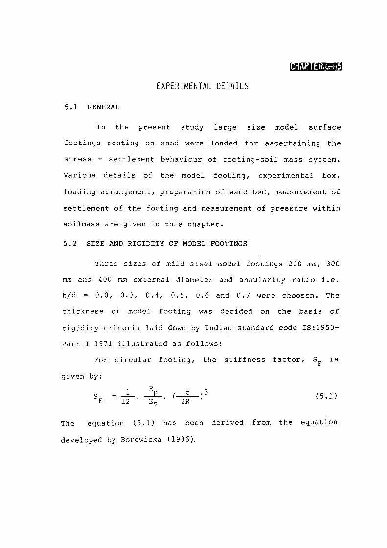
EXPERIMENTAL DETAILS

5.1 GENERAL

In the present study large size model surface

footings resting on sand were loaded for ascertaining the

stress - settlement behaviour of footing-soil mass system.

Various details of the model footing, experimental box,

loading arrangement, preparation of sand bed, measurement of

settlement of the footing and measurement of pressure within

soilmass are given in this chapter.

5.2 SIZE AND RIGIDITY OF MODEL FOOTINGS

Three sizes of mild steel model footings 200 mm, 300

mm and 400 mm external diameter and annularity ratio i.e.

h/d = 0.0, 0.3, 0.4, 0.5, 0.6 and 0.7 were choosen. The

thickness of model footing was decided on the basis of

rigidity criteria laid down by Indian standard code 15:2950"-

Part I 1971 illustrated as follows:

For circular footing, the stiffness factor, S is

given by:

The equation (5.1) has been derived from the equation

developed by Borowicka (1936).

79

where

E = Young's modulus of elasticity of footing P

material in k Pa

E = Young's modulus of dfeisticity of the foundation

sand in k Pa

t-h - Thickness of the footing in mm

R = Radius of footing in mm

Since E for sand changes continously with increase S 3 J

in the depth and with the change in load level, a

representative value of E is required. It has been found

that, for circular footings on sand beds,the stress in sand

at depth of 0.6 times the diameter can be taken as the

average of the stresses in the entire meuium/ Arora (1980

and 1984). The value of E corresponding to the in-situ s r 3

stress condition at this depth was taken as representative value E = 6 x 10^ k Pa

s

The value of E is determined by conducting the s

triaxtd tests in the laboratory according to IS: 2720 Part

XI-1971. This value of E has been used for computation of

S . For rigid footing, S_ should be greater than 0.1.

r F When E = 6 x lo" kPa

s Q

E =2.0 X 10 k.Pa (mild steel plate was used)

th = 20 mm (thickness assumed)

R = 200 mm.

80

Substituting above values in equation (5.1)/ we get

S^ = 0.27 > 0.1.

The behaviour of annular footing is neither perfectly

circular footing nor strip footing, therefore it was felt

necessary to check the rigidity of annular footing as strip

footing. The following Browicka's (1939) equation in the

modified form has been used for this purpose.

S, = ^ 3 ^ (-yi-)3 F 12 E3 B

where B = width of strip footing

In case of 400 mm diameter annular footing of annularly ratio

= 0.7, B = 60 mm.

S^ = 5.14 > 0.1 r

and also for h/d = 0.3, B = 140 mm

S^ = 0.81 > 0.1 r

Hence the model footings were prepared using 20 mm

thick mild steel plates so that the footings behave as rigid

footings. The annular plate was mounted with a similar solid

plate with the help of 100 mm x 40 mm x 20 mm vertical legs

for transfering the load to the footing plate. A close up

photo of the models used is shown in Fig. (5.1) and

schematic diagram of model annular footing has shown in Fig.

(5.2). The steel plate at the top was grooved to accomodate

(81)

FIG.5.1-PH0T0GRAPH OF MODEL FOOTINGS

82 EXTERNAL DIA.

d

VERTICAL MEMBER

I.JV777?

BOTTOM PLAN

1 iLiJlfi ^

VERTICAL

MEMBER

BOTTOM PLATE

20 mm. THICK

ANNULAR PLATE

TOP PLATE

SECTION A A

FIG.5.2-DETAILS OF MODEL OF ANNULAR FOOTING

ALL DIMENSIONS IN mm.

MATERIAL USED 20mm THICK M.S.SHEET

83

a ball such that a model can be centred with the proving

ring and load applied eccentrically. To simulate the

roughness of the actual footing, the base was made rough

according to IS Code: 1888 - 1982.

5.3 EXPERIMENTAL BOX

A rigid steel tank 2.0 m x 2.0 m x 1.0 m internal

dimensions was designed and prepared for accomodating the

bed of sand Fig. (5.3). The size of the tank was selected in

order to keep the rupture zones and pressure bulb within

boundaries. The tank was prepared with 4 mm thick steel

plate and angle iron of 35 mm x 35 mm size. The steel tank

was kept on a steel girder portal self straining loading

frame which was designed for the purjpose of loading

arrangement. The tank was rested on four steel girders of

loading frame 150 mm above the ground. The top of the girder

was fabricated in such a way that it can be used for placing

the pxoving ring and jack to be centre of the tank so that

the load application by hydraulic jack would always be on

the centre of the tank.

5.4 LOADING ARRANGEMENT

The schemetic diagram of experimental set with

loading arrangement has shown in Fig. (5.4). Steel girders

were welded to suitably designed portal frame as shown in

84

2000

PLAN

500

OF

500 500 500

DF qoF 2000

ELEVATION

-^75 k CHANNEL =a

ALL DIMENSIONS IN mm.

FIG.5.3- DETAIL OF SAND BOX

1000

i so

. T

85

1750

350

ISO-750 • PIPE

900

r-H-! I—I '

1750

Ul -H3S0 k -

)S0

• 2000 -25000

M - t r = * _ _ j

PLAN

1520

2300

IZ

Z "a/

/6/

RSJ 300X150

RSJ 300X150

STEEL BALL

PROVING RINO

FLOOR

a

A a N r ^

1

DIAL ' ^ l l ^ Cp-^ GAUGE U O ; [ [ J j _ 'ÔDEL

SAND BOX

2000X2000X1000

RSJ 300X150

O

190

L y Nr" Sr ' t 300

1. i. / z RSJ 300X150

T 4S0

J 4L-

4 SO

RSJ 300X150

,JZA1

3650

rr

1 ^ 3 7 5 - ^ ALL 0IMCNSION5 IN mm

SECTIONAL ELEVATION

FIG.S.A- DETAILS OF EXPERIMENTAL SET-UP

(86)

FIG.5.5-PHOTOGRAPH OF LOADING ARRANGEMENT AND MODEL FOOTING

(87)

FIG.5.6-PHOTOGRAPH SHOWING LOADING FRAME, STEEL TANK AND HYDRAULIC JACK

88

Fig. (5.5) and (5.6). A steel joist was bolted across the

steel girders to support the reaction of hydraulic jack. The

jack was adjusted just above the centre of the footing. A

proving ring of 50t capacity was used to measure the load

applied. Load were applied to the footing through a remote

control hydraulic jack as shown in Fig. (5.5 & 5.6).

5.5 SOIL USED

In this study, medium uniform river sand was used.

The grain size distribution curve is shown in Fig. (5.7).

The properties of the above mentioned sand used are as

follows: TABLE 5-1 PROPERTIES OF SAND

Fine fraction • 17%

Medium fraction 80%

Coarse fraction 3%

Uniformity coefficient/ C 1.47 u

Coefficient of curvature, C 1.14 c

Effective size, D. 0.17 mm

Specific gravity, G 2.65

Average bulk unit weight, Y 162 kPa

Angle of internal friction, < 42"

According to Indian standard code IS: 1498 - 1970

the soil is- poorly graded sand (SP). The angle of

shearing resistance was obtained from triaxial shear

test for confining pressure from 50 to 100 KPa.

89

2

UJ O <

z u a a

l U U

90

80

70

60

50

40

30

->f\ iO

i n 1 U

0 • IL I

^ < ' / . t

n : T . t . t . 1 Cu =

i T <:c= r : r . t _ , ., i

...Zl ..7: ,r 1

1 060 , 0.4

D10 ' 0 . 1

= 1.4

!5 7

7

1 1 0.01 0.1 1 GRAIN SIZE,(mm)

FINE i MEDIUM j COARSE SAND

10

Fig.5.7-Particle size distribution for sand

90

Vibration technique can not be used for obtaining a

uniform density of sand when earth pressure cells are to be

embeded in it. Raining techniques are quite suitable in such

conditions, Walker and Whitker (1967).

5.6 MEASUREMENT OF THE SETTLEMENT

In order to record the correct settlement of the

footing for each increment of load applied, four sensitive

dial gaugesof least count .01 were placed on the top loading

plate directly under the proving ring on the peripheries at

an angle of 90° to each other. The dial gauges were mounted

on magnetic bases were placed on two independent reference

bars on two sides of the footing Fig. (5.8). Four dial

gauges on four sides were placed in such a way as to record

any uneven settlement that may take place. An average

settlement was obtained from the settlement recorded by all

the four dial gauges for each increment of load applied.

The tank was filled by rainfall technique in layers

of 100mm. The height of fall has to be known for attaining a

particular density. In order to achieve the required density

by rainfall technique a graph was plotted between the height

of the fall versus density Fig. (5.9). It was observed that

the relative density increases as the height of the fall

increases, but beyond a fall of 900 mm there is almost no

increase in the relative density. At an average fall of 850

(91)

FIG 5.8-PHOTOGRAPH SHOWING PLACEMENT OF DIAL GAUGES ON MODEL FOOTING

92

E u

< u. u. O t -I o ijj X

10 20 30 40 50 60 70 80 90 100

RELATIVE DENSITY ( Percent )

Fig.5.9- Height of fall versus relative density

93

mm the maximum relative density achieved was 75 percent. The

sieve was first set at the required height and when one

layer of 100 mm was laid, sieve is lifted by the same

distance so that the same fall is provided throucôut the

filling. After the sand was filled the surface is levelled

and the footing was placed properly on it for the test. When

the test was completed the sand from the tank was removed

and refilled by the same technique for the next test. During

the process of filling of tanks, samples were also taken to

ascertain the required relative density of sand deposit.

5.7 ME/iSUREMENT OF PRESSURE IN THE SOIL MASS

For determination of stresses in the sand mass at

various depths below the centre line of the footing, eight

free earth pressure cells were embeded at depths of 0.2q and

0.5q i.e. significant depth, when q is the intensity of

pressure, below the surface of the footing depending upon

the size and annularity of the footing. These pressure cells

were placed on sand with their diaphragms at bottom. As soon

as the required level of sand was attained during the

process of deposition of sand, the leads of the strain

gauges of the earth pressure cells were taken out

horizontally towards the side wall of the tank. The process

of depsotion of sand was continued after the pressure cells

had been placed. These pressure cells were connected to a

94

Switching Balancing Unit (S.B.U.) and the S.B.U. was

connected to Universal Indicater model UA6411B digital

display for displaying out put of the pressure cells made by

New Engg. Enterprise/ Roorkee (India) as shown in Fig. 5.10

and Fig. 5.11.

The pressure cells of known calibration factors were

used for measuring the stresses in the sand at various

depths. The leads in 4 number from each cells (2 for

excitation and 2 for out put) v ere taken out side. They v;ere

of different colours. The leads of the pressure cells were

connected to the 1st channel's knobs in 4 nos. of the same

colour. The excitation leads were connected to Bridge

terminal 2 and 3 and out put leads to Bridge terminal 1 and

4. The Unit consists of 10 channels. Eight channels were

used for eight pressure cells. The switching and balancing

unit was connected to the digital universal indicater. After

balancing the universal indicater and Switching and

Balancing unit, the stress v;as measured by noting the

reading which appeared on digital display and multiplied by

the respective calibration constant.

The salient features about pressure cell, switching

balancing unit and universal indicater have been discussed

in Appendix-B.

(95)

FIG.5.10-PHOTOGRAPH SHOWING SWITCHING BALANCING UNIT,UNIVERSAL INDICATOR AND VOLTAGE STABILIZER

(96)

FIG.5.11-PHOTOGRAPH SHOWING UNIVERSAL INDICATOR,S.B. UNIT CONNECTED WITH PRESSURE CELLS( Embedded in the tank)

CHAPTER^m

TEST RESULTS AND DISCUSSION

6 . 1 SHEAR STRENGTH PTUIAMETERS

In this study dense sand was used. Hence the value of

c (cohesion) is equal to zero. The angle of shearing

resistance 0 was determined by conducting triaxial tests in

the laboratory for approximately the same density as that of

the sand in the experimental box. The mohr's circle diagram

is shown in Fig. 6.1 The average value of 0 = 42° was

determined.

6.2 LOAD INTENSITY VERSUS SETTLEMENT OF MODEL FOOTINGS

The load intensity-settlement was observed for each

test using 200 mm, 300 mm and 400 mm external diameter

circular and annular model footings each with six different

annularity ratios (h/d) = 0.0, 0.3, 0.4, 0.5, 0.6 and 0.7.

These footings were tested on a constant density of dry sand

deposited in a tank. The load intensity versus settlement

results are presented in the form of curves, shown in Fig.

6.2, 6.3 and 6.4. which indicate that the initial slope of

the curves for solid circular footing i.e. h/d = 0.0 is less

than the annular footings having h/d > 0. The settlement for

the same stress level near elastic range is more for smaller

h/d ratio. This happens due to larger pressure bulb

available to solid circular footing and footings with

98

o a M

•» «n

cc t -«/i

a: <

700

600

SOO

400

300

^ 200

100

Shear strength parameters C = O , 0 = 42«

100 200 300 400 500 600 700 800

NORMAL STRESS, kPg

Fig.6.1-Mohr diagram circle

LOAD INTENSITYjkPa

99

100 200 300

E

2

to

2 -

4 -

6 -

8 -

10

-

"•

s —

1

I 1 1 1

^^^S^ , . , ^^^h /d r0 .6

^ ^ J ^ ^ h / d = 0.5

Ôy—h/d:0.3

h/d=0.4 P \

h /d :0 .0

I I I !

-

^

Fig.6-2 Load intensity- settlement curves tor 200 mm external diameter footing

LOAD INTENSITY,kPQ

100

£ E

z l i j

z UJ

c

2

4

6

8

10

1 •)

I

-

100 ^ __ 1

1

1

1

200 300 3C 1 1 1 1

h/drO.7

^ j - ^ . ^ ^ h/d=X).6

^sN55v,^h/dr0.5

h/d=0.4 " ^ NV

\ \ v -h /d - -0 3

h/dr0.0 jL

1 1 1 1

Fig.63 Load intensity-sett lement curves for 300 nr>m external diameter tooting

LOAD INTENSITY,kPa

101

£ e

2

UJ

UJ

if)

Fig. 6.4 Load intensi ty - sett lement curves for AOO mm external diameter footing

102

smaller h/d ratios as compared to annular footings of larger

h/d ratios.

6.3 ULTIMATE BEARING CAPACITY

Ultimate bearing capacity q versus size of the

footing with different annularity ratio has been plotted in

Fig. 6.5. The results show that for the same annularity

there is an increase in ultimate bearing capacity as the

size of the footing increases. In can be further observed

that the ultimate bearing capacity decreases as the

annularity ratio increases.

6.4 SRAPE FATOR Sf

To cater for the annularity an attempt has been made

to suggest shape factor for annular footing resting on sand

bed. It is intended to introduce a shape factor Sy in

Terzaghi's ultimate bearing capacity relationship for strip

action of annular footing resting on the surface of the sand

as under:

q = 0.5 y B Ny S/ (6.1)

The shape factors for 200 mm, 300 mm and 400 mm size

footing having h/d = 0.0, 0.3 0.4 0.5, 0.6 and 0.7 were

calculated using the above equation and observed values of

q , for if = 42° and corresponding bearing capacity factor

Ny = 150. Tne shape factor versus annularity ratio plot is

1 0 3

Q?

< a < u o 2 cr < Ui CD UJ

500

400

300

200

< 5 100

•

h 0 X

A

X

h/d=0.0 h/drO.3 h/d s 0. A h/d=0.5 h/d =0.6 h/d = 0.7

100 200 300 400

FOOTING DIAMETER, mm

Fig.6.5 Ult imate bearing capacity q^ Vs. diameter of footing

for different values of ' h / d *

104

A.O

35 -

3,0 -

cr o » -o <

< X in

2.5 -

1.5

1.0

0.5

0.0

1 1 1 1 1 1 1

V^^ ^— Sy= 1.86 ( 1 + h / d )

LEGEND - External footing -

Diameter 0 200mm

_ X 300mm

A 00

1 1 1 1 1 1 1 0.0 0.1 0.2 0.3 O.A 0.5 0.6

ANNULARITY RATIO, ( h / d )

0.7 0.8

Fig.6.6 Shape factor (Sy) Vs. Annularity ratio ( h / d )

105

shown in Fig. 6.6. It is evident from the figure that the

shape factor depends on h/d ratio of the footing and it is

almost independent of size of the footings. Based on the

experimental results of the plot shown in Fig. 6.6, the

author has developed an empirical equation for shape factor

(by feeding the data in computer and using least square

method) as given below:

Sy = 1.86 (1+h/d) (6.2)

for 0 h/d -$ 0.7

By substituting the shape factor from equation (6.2)

in equation (6.1)/ the equation for ultimate bearing

capacity of annular footings reduces to:

q = 0.465 y.d [l-(h/d)^j (6.3)

for 0 h/d ^0.7

6.5 NON DIMENSIONAL PARAMETER< (q /V.d) VERSUS ANNULARITY û

RATIO, (h/d)

The non-dimensional form of the ultimate bearing

capacity equation derived in Chapter 4 is reproduced below:

(q /Yd) = 0.2.5 (l-h/d) Ny. Sy for h/d ,$: 1 u Theoretical ' y r

Using N^ = 150 for 0 = 42° and Sy = 1.86 (1+h/d) in the

right hand side of the equation, the above equation reduces

to:

(q /^d) _ - . = 70 [1-h/d)^] (6.4) u Theoretical

106

for 0 h/d <$ 0.7

Theoretically there should be a unique relationship

between q //d versus h/d which is confirmed by the equation

given above. Non-dimensional parameter (q //d) , , has ^ ^ û observed

also been calculated on the basis of observed ultimate

bearing capacity q for 200 mm, 300 mm and 400 mm diameter

footing having h/d = 0.0, 0.3, 0.4, 0.5, 0.6 and 0.7, using

" = 162 kPa. Non-dimensional parameters (q /^d) , •, and '^ û observed

^V^^^Theoretical ^^^ Plotted in Fig. 6.7. (q^,/yd)^^^3î^^ and (q /Yd) , _, are in fairly good agreement,

u observed ' The values of (q / V'd)^^ ^. , given by Kakroo

û' Theoretical ^

(1985) have also been plotted in Fig. 6.7 and compared with

the author's values. The theoretical equation derived by

Kakroo for dense sand is given below:

^V^^^Theoretical " 0. 36[ 236+465(h/a)-1420(h/d) +754

(h/d)^] (6.5)

The results are in fairly good agreement qualitatively.

107

100

18 t

^ 80

0

60

50

AO

30 -

(û/yd)s0.36D36 •f5(h/d)-U20(h/df

7 5 A ( h / d / ] -Kakroo's equation

( ^ u A d Ôbserved EXTERNAL FOOTING DIAMETER 200 mm. 300 mm. AOOmm. Kakroo's values

(%/2 rd )=70n- (h /d ) * l

Author's equation

20 I

0.0 0.1 0.2 0.3 0.4 0.5 ANNULARITY RATIO h/d

0.6 0.7 o.e.

Fig.6.7 Non- dimensional parameter ( qn / yd ) Vs. Annularity ratio f h / r f i ^ / • bbserved

STRESS ANALYSIS

The bearing capacity of soil-foundation system is

governed mostly by settlement criteria in case of sandy

soils. The settlement of the foundation depends on the

stress condition in the soil below the foundation.

Boussinesq's classical equation is generally used for

computations of stresses in the soil mass. Boussinesq's

equation assumes the material to be elastic, homogeneous and

isotropic. Though the soils are not truly elastic/ yet the

equation has profusely been used in Geotechnical

Engineering. The use of Principle of superposition and

Numerical Integration has been suggested for determination

of stresses under a uniformly loaded annular footings.

7.1 PRINCIPLE OF SUPERPOSITION METHOD

The principle of superposition state that if y, is

the effect of Q-^ and y is the effect of Q^ the combined

effect of Q, + Q- will be y, + y-,. On the basis of

principle of superposition, the stresses below the footing

has been computed considering the full diameter 'd' of the

footing and deducting the stresses due to annular portion of

the footing having, diameter 'h'. The superposition is

explained in Fig. 7.1. For example, considering 400 mm

diameter footing of annularity ratio h/d = 0.3, the value of

109

-H-d—4 f-hH

a..Ûwnrl - cn TTITT

g i

fM l u l j 111 I

= ^1 - ^ 2

Fig. 7.1- Principle of superposition for annular fooling

l l u

b cr

c o

•4-»

J3

E o

c

3

O

3 t -

u L. 0* > o

• o a _o

"5 E t -o z:

<7»

> O I . o en

UJ u. 0*

N O

<N

Ill

h = 120 mm. First, the stresses have been worked out for 400

mm diameter circular footing at various depths considering

uniformly distributed load of intensity 'g' over entire area

by the footing. Egorov (1977), Fig. 7.2. The Egorov plot

represents various curves drawn for r/a = 0 to r/a = 2.0

where 'r' is the distance of point where stresses is being

computed from the centre of the footing and 'a' is the

radius of the footing. These curves have been drawn between

c /q versus Z/a where og- is the stress at a depth 'Z' where

stress v\7as to be found out. The values of Z, in this study

was chosen from 20 mm to 500 mm at interval of 20 mm

depending upon the significant depth of isobars. Similarly

the annular portion is considered as complete circular

footing of 120 mm diameter (h = 120 mm) and the stress is

worked out at the same depth as considered for 400 mm

diameter of footing. The difference of these stresses will

be net stress due to annular footing of 400 mm diameter of

annularity ratio 0.3. Table 7-1 to 7-5.

By using same priciple/ stresses have been worked out

for 400 mm diameter annular footing of h/d ratios, 0.4,

0.5, 0.6 and 0.7 and the same have been given in the

tabular form (Table 7-6 to 7-25). In the same way the

stresses can also be calculated for 300 mm and 200 mm

diameter annular footings.

112

VERTICAL STRESS UNDER ANNULAR FOOTING THEORETICALLY MEASURED

BY SUPER POSITION METHOD

ANNULARITY RATIO

EXTERNAL RADIUS

INTERNAL RADIUS

0.3

200.0 mm

60.0 mm

RADIAL DISTANCE

TABLE NO. 7-1

200.0 mm

S.No. Depth mm

Sigma - z/q

1

2

3

4

5

6

7

8

9

10

11

12

13

14

15

16

17

18

19

20

20

40

60

80

100

120

140

160

180

200

220

240

260

280

300

320

340

360

380

400

0.48

0.46

0.44

0.42

0.40

0.38

0.36

0.34

0.32

0.31

0.29

0.27

0.25

0.24

0.23

0.22

0.21

0.19

0.18

0.17

113

TABLE NO. 7-2

RADIAL DISTANCE 150 mm

S.No. Depth Sigma - z/q mm

1 20 0.97

2 40 0.92

3 60 0.79

4 80 0.70

5

7

100 0.65

^ 120 0.57

140 0.52

8 160 0.50

9 180 0.45

10 200 0.42

11 220 0.39

12 240 0.34

13

14

15 300 0.28

260 0.32

280 0.29

16

17

18

19

20 400

310 0.26

320 0.25

340 0.23

360 0.21

0.20

114

TABLE NO. 7 3


S.No. Depth Sigma - Z/q mm

1 20 0.97

2 40 0.92

3 60 0.85

4 80 0.78

5 100 0.72

6 120 0.67

7 140 0.60

8 160 0.54

9 180 0.52

10 200 0.48

11 220 0.43

12 240 0.41

13 260 0.37

14 280 0.34

15 300 0.33

16 320 0.32

17 340 0.28

18 360 0.26

19 380 0.24

20 400 0.23

21 420 0.21

22 440 0.19

115

TABLE NO. 7-4

RADIAL DISTANCE 80.0 mm


1 20 0.92

2 40 0.83

3 60 0.77

4 80 0.73

5 100 0.70

6 120 0.67

7 140 0.63

8 160 0.59

9 180 0.54

10 200 0.50

11 220 0.47

12 240 0.43

13 260 0.40

14 280 0.38

15 300 0.34

16 320 0.32

17 340 0.30

18 360 0.28

19 380 0.25

20 400 0.23

21 420 0.22

22 440 0.20

23 • 460 0.19

116

TABLE No. 7-5

RADIAL DISTANCE 0.0 nun

S.No. Depth Sigma - . Z/q mm

1 20

2 40

3 60

4 80

5 100

6 120

7 140

8 160

9 180

10 200

11 220

12 240

13 260

14 280

15 300

16 320

17 340

18 360

19 380

20 400

21 420

22 440

23 460

0 0 0

0

0

0

0

0

0

0

0

0,

0,

0.

0.

0,

0.

0.

0.

0 .

0 .

0.

0 .

0 .

.03

.16

.32

.42

.53

.51

.55

.54

.55

.52

.49

.46

.43

.39

,37

35

31

29

26

24

23

22

20

117


ANNULARITY RATIO

EXTERNAL RADIUS

INTERNAL RADIUS

RADIAL DISTANCE

TABLE NO. 7-6

0.4

200.0 mm

80 mm

200.0 mm

S.No, Depth mm

Sigma-Z/q

1

2

3

4

5

6

7

8

9

10

11

12

13

14

15

16

17

20

40

60

80

100

120

140

160

180

200

220

240

260

280

300

320

340

0.46

0.45

0.44

0.41

0.39

0.36

0.34

0.31

0.30

0.29

0.28

0.27

0.24

0.22

0.21

0.20

0.19

118

TABLE NO. 7 - 7

Ri>X)IAL DISTANCE 1 5 0 . 0 mm

S . N o . D e p t h S i g m a - Z / q mm

1 20 0.96

2 40 0.92

3 60 0.78

4 80 0.69

5 100 0.63

6 120 0.54

7 140 0.50

8 160 0.47

9 180 0.46

10 200 0.45

11 220 0.44

12 240 0.31

13 260 0.30

14 280 0.27

15 300 0.26

16 320 0.24

17 340 0.23

18 360 0.21

19 380 0.19

119

S.No,

1

2

3

4

5

6

7

8

9

10

11

12

13

14

15

16

17

18

19

20

TABLE NO. 7-8


mm

20

40

60

80

100

120

140

160

180

200

220

240

260

280

300

320

340

360

380

400

Sigma - Z/q

0

0

0

0

0

0

0

0

0,

0,

0.

0.

0.

0.

0.

0.

0.

0.

0.

0.

.91

.81

.74

.67

.62

.58

.52

.47

.45

.43

,40

,37

.34

,31

30

29

25

24

22

21

120

TABLE NO. 7-9



1 20 0.54

2 40 0.56

3 60 0.58

4 80 0.57

5 100 0.55

6 120 0.54

7 140 0.53

8 160 0.49

9 180 0.47

10 200 0.44

11 220 0.41

12 240 0.39

13 260 0.35

14 280 0.33

15 300 0.30

16 320 0.28

17 340 0.26

18 360 0.24

19 380 0.23

20 400 0.21

21 420 0.20

22 440 0.18

121

TABLE NO. 7-10


S.No. Depth Sigma - Z/q run

1 20 0.01

2 40 0.08

3 60 0.15

4 80 0.14

5 100 0.37

6 120 0.41

7 140 0.40

8 160 0.45

9 180 0.46

10 200 0.44

11 220 0.42

12 240 0.39

13 260 0.37

14 280 0.34

15 300 0.32

16 320 0.31

17 340 0.28

18 360 0.26

19 .80 0.23

20 4 0 0.22

21 420 0.21

22 440 0.19

122

VERTICAL STRESS UNDER ANNULAR FOOOTING

ANNULARITY RATIOO 0.5

EXTERNAL RADIUS 200.0 mm

INTERNAL RADIUS 100.0 mm

TABLE NOP. 7-11

RADIAL DISTANCE 200.0 ram

S.No. Depth . Sigma- Z/q mm

1 20 0.47

2 40 0.45

3 60 0.43

4 80 0.40

5 100 0.38

6 120 0.35

7 140 0.32

8 160 0.30

9 180 0.27

10 200 0.26

11 220 0.25

12 240 0.23

13 260 0.22

14 280 0.20

15 30C 0.18

123

TABLE NO. 7-12


S.No. Depth min

1. 20

2. 40

3. 60

4. 80

5. 100

6. 120

7. 140

8. 160

9. 180

10. 200

11. 220

12. 240

13. 260

14. 280

15. 300

16. 320

17. 340

Sigma - Z/q

0

0

0,

0,

0,

0,

0,

0.

0.

0.

0.

0.

0.

0.

0 .

0 .

0 .

.95

.89

.73

.61

.56

.53

.50

.42

.38

.34

.32

,30

,27

23

22

21

19

124

TABLE NO. 7-13


S.No. Depth Sigma - Z/q

1. 20 0.53

2. 40 0.54

3. 60 0.54

4. 80 0.53

5. 100 0.49

6. 120 0.48

7. 140 0.43

8. 160 0.42

9. 180 0.32

10. 200 0.33

11. 220 0.32

12. 240 0.30

13. 260 0.27

14. 280 0.26

15 300 0.25

16. 320 0.23

17. 340 0.22

18. 360 0.20

19. 380 0.19

20. 400 0.18

125

TABLE NO. 7-14



1 .

2 .

3 .

4 .

5.

6.

7.

8 .

9.

10 .

1 1 .

1 2 .

1 3 .

14 .

15.

16 .

17.

18 .

19 .

20 .

20 0.12

40 0.28

60 0.37

80 0.41

100 0.42

120 0.43

140 0.42

160 0.40

180 0.39

200 0.38

220 0.33

240 0.32

260 0.30

280 0.28

300 0.26

320 0.24

340 0.23

360 0.21

380 0.20

400 0.18

126

TABLE NO. 7-15


S.NO. Depth Sigma - Z/q

1. 20 0.01

2. 40 0.06

3. 60 0.10

4. 80 0.19

5. 100 0.26

6. 120 0.33

7. 140 0.32

8. 160 0.35

9. 180 0.30

10. 200 0.36

11. 220 0.35

12. 240 0.33

13. 260 0.32

14. 280 0.28

15. 300 0.27

16. 320 0.26

17. 340 0.24

18. 360 0.22

19. 380 0.21

20. 400 0.20

127


ANNULARIY RATIO 0.6



TABLE NO. 7-16



1. 20

2. 40

3. 60

4. 80

5. 100

6. 120

7. 140

8. 160

' 9. 180

10. 200

11. 220

12. 240

0.47

0.44

0.42

0.38

0.34

0.31

0.27

0.25

0.24

0.22

0.21

0.19

128

TABLE NO. 7-17



1. 20 0.95

2. 40 ' 0.83

3. 60 0.69

4. - 80 0.54 5. 100 0.48

6. 120 0.40

7. 140 0.34

8. 160 0.32

9. 180 0.29

10. 200 0.26

11. 220 0.24

12. 240 0.22

13. 260 0.21

14. 280 0.19

129

TABLE NO. 7-18



1- 20 0.52

2. 40 0.52

3- 60 0.50

4. 80 0.46

5. 100 0.43

6. 120 0.40

7. 140 0.37

8. 160 0.31

9- 180 0.31

10. 200 0.29

11. 220 0.27

12. 240 0.25

13. 260 0.23

14. 280 0.21

15. 300 0.20

16. 320 0.19

130

TABLE NO. 7-19



1. 20 0.01

2. 40 0.07

3. 60 0.16

4. 80 0.19

5. 100 0.25

6. 120 0.30

7. 140 0.29

8. 160 0.29

9. 180 0.28

10. 200 0.27

11. 220 0.26

12. 240 0.25

13. 260 0.23

14. 280 0.22

15. 300 0.21

16. 320 0.20

17. 340 0.19

18. 360 0.17

131

TABLE NO. 7-20



1. 20

2. 40

3. 60

4. 80

5. 100

6. 120

7. 140

8. 160

9. 180

10. 200

11. 220

12. 240

13. 260

14. 280

15. 300

16. 320

17. 340

18. 360

0

0

0

0

0

0

0

0

0,

0,

0.

0.

0,

0.

0 .

0 .

0 .

0 .

.04

.02

.07

.12

.17

.22

.25

.27

,26

.27

,27

,26

24

23

22

21

19

18

132


i\NNULARITY RATIO 0.7



T2\BLE NO. 7 - 2 1

:RADIAL DISTANCE 2 0 0 . 0 mm

S . N o . D e p t h Sigma - Z / q mm

1. 20 0.47

2. 40 0.43

3. 60 0.36

4. 80 0.30

5. 100 0.27

6. 120 •0.21

7. 140 0.22

8. 160 0.21

9. 180 0.19

10. 200 0.18

133

TABLE NO, 7-22



1. 20 0.52

2. 40 0.50

3. 60 0.45

4. 80 0.40

5. 100 0.36

6. 120 0.31

7. 140 0.28

8. 160 0.26

9. 180 0.22

10. 200 0.21

11. 220 0.19

12. 240 0.18

134

TABLE NO. 7-23



1. 20 0.03

2. 40 0.14

3. 60 0.20

4. 80 0.24

5. 100 0.26

6. 120 0.27

7. 140 0.25

8. 160 0.24

9. 180 0.23

10. 200 0.21

11. 220 0.20 12. 240 0.19

135

TABLE NO. 7-24



1. 20

2. 40

3. 60

4. 80

5. 100

6. 120

7. 140

8. 160

9. 180

10. 200

11. 220

12. 240

0

0

0

0

0.

0.

0.

0.

0.

0.

0 .

0 .

. 01

.03

.07

.15

.18

.19

.20

,22

,21

20

20

19

136

TABLE NO. 7-25


S.No. Depth mm

1. 20

2. 40

3. 60

4. 80

5. 100

6. 120

7. 140

8. 160

9. l JO

10. 2C0

11. 22)

12. 240

13. 26(..

14. 280

Sigma

0

0

0

0

0

0.

0,

0,

0.

0.

0 .

0 .

0 .

0 .

- Z/q

.01

.02

.05

.10

.14

.16

.18

.19

.20

,21

20

19

18

17

137

7.2 NUMERICAL INTEGRATION METHOD

Stresses in the soil under an annular footing

carrying uniformly distributed load of intensity 'q' are

evaluated numerically using Boussinesq relationship. Annular

footing is divided into concentric annular rings of

thickness 'dr' and inner radius being 'r'. A small element

in this annular ring subtending an angle 'd9' at the centre

is considered as a point load for the evaluation of stresses

at a general point P in the soilmass (Fig. 7.8). The point P

is located at a depth Z and is at a radial distance R. Total

effect of the annular loaded area is obtained by integrating

the stress due to elemental load over whole of the loaded

area as given below:

d/2 2 ; f_^ i^L^ o-„ - _ l a 2A f ô [l+(r/Z)2j5/2

Rl= h/2

3q d/2 J- RidfAe f O ^^2 5/2

Rl=h/2 [l-^{r/zrV^^ (7.1)

where r = ^R2 + 1 ~ 2RRi Cos e

The above equation (7.i) has been integrated

numerically by converting it into the following form:

dA £

180 Ri

3_

R=h/2 e=0 [ l + ( r / Z ) 2 ] 5 / 2

n i n2 R.+ i 8^

i=0 j=0 [ l + ( r / Z ) 2 ] 5 / 2

1 ^ SL.

138

where rii and n„ are the number of dimensions in

radial and circumferential direction respectively. A

software programme has been developed; using the above

algorithm and has been presented in Appendix C.

The stresses worked out at various radial distances

and depths for different annularity ratios 0.3; 0.4; 0.5;

0.6 and 0.7 for 400 mm outer diameter annular footings have

been given in Table 7-26 to 7-50 and the same have been

plotted in the form of isobars in Fig. 7.3, 7.4, 7.5, 7.6

and 7.7. In the same way the isobars can also be drawn for

300 mm and 200 mm diameter annular footings. Isobars have

also been drawn for circular footing (h/d = 0.0),Table 7-51 400 VriTn

to 7-55,of,dianeter in Fig. 7.3 for comparing with (h/d=0.3)

p annular footing. These stresses comuted by this method are

almost same as calculated by superposition method.

7.3 MEASUREMENT OF STRESSES AND COMPARISON WITH THEORETICAL

VALUES

In order to verify the results of the computation of

stresses using the principle of superposition and numerical

integration the stresses have been measured in the soilmass

experimentally under annular footings of diameter 400 mm

having annularity ratios of 0.3, 0.4, 0.5, 0.6 and 0.7.

Pressure cells were used at depths of 0.2 q and 0.5 q

estimated by stress analysis as explained in Article 7.2

139

v/here q is the intensity of Load. The verification was done

for q = 50 k Pa and 100 k Pa. The location of pressure cells

have shown in Fig. 7.9.

The observed vertical stresses measured by pressure

cells have been given in Table 7-56 to 7-60. The calibrated

pressure cells of known calibration factor K supplied by New

Engg. Enterprise (Roorkee) have been used. Full arrangement

for measuring the stresses have been given in Chapter 5/

para 5.7.

The experimental values of o—2/q have also been

compared with the theoretical values of stresses computed by

software programme given in Appendix -C as represented in

the table 7-56 to 7-60. There is not much difference between

theoretical and experimental values but the theoretical

stresses are more than the experimental stresses. Therefore/

the stresses under the annular footing can be predicted

safely by this technique.

The observed values of o-g /q have also been compared

with the theoretical values by plotting a graph between oj/q

versues Z/B (where B = — - — ) . The comparison of theoretical

and measured stresses for 400 mm diameter footings for h/d

ratio 0.3, 0.4, 0.5', 0.6 and 0.7 have been shown in Fig.

7.10 to 7-14.

14C

Fig.7.3-Compansion of isobars for solid circular and annular footing of ÔOmm diameter (h /d=0 .3 )

141

Fig.y.A- Isobars for annular fooling of 400mm diameter ( h/d =0.A )

d-h •d/2

M •M 142

GL )A\r,Kvr •

_ M i W i i i i rv-Q stress"

_d_ 2

d

Fig.7.5-Isobars for annular footing of AOOmm diameter {h/d=0.5 )

h — ^ — + ''A ''A

14?.

, ^ ^ n H n i i rq stress

6_ 2

d

Fig.7.6'- Isobars for annular footing of AOOmm diameter ( h / d =0-6 )

f-^-f d/ j

^ ^ •

, , S , U I 1 1 1 i I l ^ q Mr>-s.<>

144

2

^ q

^ ^

Fig. 7.7-Isobars for annular footing of AOOmm diometer (h/d=0.7 )

14 5

Fig.7.8 Plan for stress below a point lying outside circular area

146

Stress For 4 0 0 m m Annular Footing

h/d=0.3 a^rlScm 8.b:^4cm h/drO.4 a'= 16cm &b'r 34cm h/d = 0.5 a= 12cm8,b'r32cnn

h/d =0.6 a'= 8 cm &b'r 28cm

h/d =0.7 a ' : 6cm 8ibr 20cm

Fig.7-9 Location of pressure cells

147

0.0

II

CQ

N

1.0

2.0

3.0

4.0

Fi9.7.10Comparison of theoretical and observed stresses for 400 mm diameter plate having h/d =0.3

T/q 148

0.0

CD M

THEORETICAL

OBSERVED

Fig.ZII-Comparison of theoretical and observed stresses for 400 mm diameter plate having h/d = 0.4

0.0

10

20

30

4.0

THEORETICAL

OBSERVED

Fig.7.12 Comparison of theoretical and observed stresses for 400mm diameter plate having h/d = 0.5

0.0

1.0

2.0

3-0

4.0

149

THEORETICAL

OBSERVED

Fig.7.13 Comparison of theoretical and observed stresses for 400 mm diameter plate having h/d = 0.6

T/q

CO

M

0.0

1.0

2.0

3.0

4.0

Fig.7.)A Comparison of theoretical and observed stresses for 400mm diameter plate having h/d =0.7

150

VERTICAL STRESS UNDER ANNULAR FOOTING (THEORETICALLY MEASURED BY COMPUTER)

AHHULARITY RATIO 0.3 mm EXTERNAL RADIUS 200.0 mm INTERNAL RADIUS 60.0 mm

Table No. 7-26


S.Ho. DEPTH SIGHA-z/q (mm)

1. 20.0 0.4679

2. 40.0 0.4586

3. 60.0 0.4424

4. 80.0 0.4234

5. 100.0 0.4031

6. 120.0 0.3825

7. 140.0 0.3622

8. 160.0 0.3426

9. 180.0 0.3239

10. 200.0 0.3061

11. 220.0 0.2894

12. 240.0 0.2736

13. 260.0 0.2587

14. 280.0 0.2447

15. 300.0 0.2315

16. 320.0 0.2191

17. 340.0 0.2073

13. 360.0 0.1963

19. 380.0 0.1860

20. 400.0 0.1762

21. 420.0 0.1671

22. 440.0 0.1585

23. 460.0 0.1505

24. 480.0 0.14?9

25. 500.0 0.1358

151

Table Ho. 7-27


S.No. DEPTH SIGMA-z/q (mm)

1.

2.

3.

4.

5.

6.

7.

8.

9.

1.0.

11.

12.

13.

14.

15.

16.

17.

18.

19.

20.

21.

22.

23.

24.

25.

20.0

40.0

60.0

80.0

100.0

120.0

140.0

160.0

180.0

200.0

220.0

240.0

260.0

280.0

300.0

320.0

340.0

360.0

380.0

400.0

420.0

440.0

460.0

480.0

500.0

0.9845

0.9175

0.8247

0.7346

0.6563

0.5905

0.5352

0.4883

0.4480

0.4128

0.3818

0.3540

0.3290

0.3064

0.2858

0.26bd

0.2497

0.2336

0.2192

0.2058

0.1934

0.1820

0.1714

0.1617

0.1526

152

Table No. 7-28


S.Ho. DEPTH SIGMA-z/q (mm)

1. 20.0 0.9847

2. 40.0 0.9292

3. 60.0 0.8604

4. 80.0 0.7935

5. 100.0 0.7311

6. 120.0 0.8735

7. 140.0 0.6206

8. 160.0 0.5720

9. 180.0 0.5276

10. 200.0 0.4863

11. 220.0 0.4495

12. 240.0 0.4154

13. 260.0 0.3842

14. 280.0 0.3557

15. 300.0 0.3297

16. 320.0 0.3059

17. 340.0 0.2842

18. 360.0 0.2645

19. 380.0 0.2464

20. 400.0 0.2299

21. 420.0 0.2148

22. 440.0 0.2010

23. 460.0 0.1884

24. 480.0 0.1768

25. 500.0 0.1661

153

Table No. 7-29


S.No. DEPTH SIGHA-z/q (mm)

1. 20.0 0.9324

2. 40.0 0.8372

3. 60.0 0.7830

4. 80.0 0.7435

5. 100.0 0.7058

6. 120.0 0.6661

7. 140.0 0.6252

8. 180.0 0.5839

9. 180.0 0.5432

10. 200.0 0.5041

11. 220.0 0.4670

12. 240.0 0.4323

13. 260.0 0.4000

14. 280.0 0.3702

15. 300.0 0.3428

16. 320.0 0.3177

17. 340.0 0.2948

18. 360.0 0.2739

19. 380,0 0.2548

20. 400.0 0.2374

21. 420.0 0.2214

22. 440.0 0.2069

23. 460.0 0.1936

24. 480.0 0.1814

25. 500.0 0.1703

154

Table No. 7-30



1. 20.0 0.0313

2. 40.0 0.1661

3. 60.0 0.3341

4. 80.0 0.4651

5. 100.0 0.5447

6. 120.0 0.5823

7. 140.0 0.5900

8. 160.0 0.5785

9. 180.0 0.5553

10. 200.0 0.5257

11. 220.0 0.4930

12. 240.0 0.4596

13. 260.0 0.4269

14. 280.0 0.3957

15. 300.0 0.3664

16. 320.0 0.3392

17. 340.0 0.3142

18. 360.0 0.2912

19. 380.0 0.2702

20. 400.0 0.2511

21. 420.0 0.2337

22. 440.0 0.2177

23. 460.0 0.2032

24. 480.0 0.1900

25. 500.0 0.1779

155



Table No. 7-31



1. 20.0 0.4677

2. 40.0 0.4571

3. 60.0 0.4382

4. 80.0 0.4157

5 100.0 0.3917

6. 120.0 0.3679

7. 140.0 0.3451

8. 160.0 0.3238

9. 180.0 0.3040

10. 200.0 0.2857

11. 220.0 0.2689

12. 240.0 0.2533

13. 260.0 0.2389

14. 280.0 0.2255

15. 300.0 0.2129

16. 320.0 0.2013

17. 340.0 0.1904

18. 360,0 0.1801

19. 380.0 0.1706

20. 400.0 0.1616

21. 420.0 0.1532

22. 440.0 0.1453

23. 460.0 0.1380

24. 480.0 0.1310

25. 500.0 0.1245

156

Table No. 7-32

RADIAL DISTANCE 150 . 0 rriin

S.No. DEPTH SIGMA-z/q

(mm)

1,

2

3.

4,

6.

6,

7.

8,

9.

10,

11.

12.

13.

14.

15.

16.

17.

18.

19.

20.

21.

22.

23.

24.

20.0

40.0

60.0

80.0

100.0

120.0

140.0

160.0

180.0

200.0

220.0

240.0

260.0

280.0

300.0

320.0

340.0

360.0

380.0

400.0

420.0

440.0

460.0

480.0

500.0

0.9829

0.9082

0.8047

0.7055

0.6214

0.5526

0.4965

0.4501

0.4110

0.3775

0.3484

0.3226

0.2997

0.2790

0.2602

0.2431

0.2274

0.2131

0.1999

0.1877

0.1765

0.1662

0.1566

0.1478

0.1396

157

Table No. 7-33



1. 20.0 0.9269

2. 40.0 0.8160

3. 60.0 0.7428

4. 80.0 0.6856

5. 100.0 0.6348

8. 120.0 0.5878

7. 140.0 0.5442

8. 160.0 0.5039

9. 180.0 0.4666

10. 200,0 0.4321

11. 220.0 0.4004

12. 240.0 0.3711

13. 260.0 0.3442

14. 280.0 0.3195

15. 300.0 0.2968

16. 320.0 0.2769

17. 340.0 0.2569

18. 360.0 0.2395

19. 380.0 0.2234

20. 400.0 0.2088

21. 420.0 0.1953

22. 440.0 0.1830

23. 460.0 0.171 J

24. 480.0 0.1612

25. 500.0 0.1516

158

Table No. 7-34


'STNOT DEPTH SIGMA-z/q (mm)

1. 20.0 0.5544

2. 40.0 0.5770

3. 60.0 0.5909

4. 80.0 0.5912

5. 100.0 0.5795

6. 120.0 0.5590

7. 140.0 0.5328

8. 160.0 0.5034

9. 180.0 0.4727

10. 200.0 0.4419

11. 220.0 0.4119

12. 240.0 0.3832

13. 280.0 0.3562

14. 280.0 0.3309

15. 300.0 0.3074

16. 320.0 0.2857

17. 340.0 0.2658

18. 360.0 0.2474

19. 380.0 0.2306

20. 400.0 0.2152

21. 420.0 0.2010

22. 440.0 0.1881

23. 460.0 0.1', o2

24. 480.0 0.1653

25. 500.0 0.1553

159

Table No. 7-35


S.No, DEPTH SIGMA-z/q (mm)

1. 20.0 0.0135

2. 40.0 0.0832

3. 60.0 0.1947

4. 80.0 0.3053

5. 100.0 0.3897

6. 120.0 0.4424

7. 140.0 0.4680

8. 160.0 0.4733

9. 180.0 0.4648

10. 200.0 0.4476

11. 220.0 0.4254

12. 240.0 0.4006

13. 260.0 0.3752

14. 280.0 0.3500

15. 300.0 0.3258

16. 320.0 0.3030

17. 340.0 0.2817

18. 360.0 0.2619

19. 380.0 0.2437

20. 400.0 0.2269

21. 420.0 0.2116

22. 440.0 0.1975

23. 460.0 0.1846

24. 480.0 0.1728

25. 500.0' 0.1620

160



Table No. 7-36



1. 20.0 0.4673

2. 40.0 0.4540

3. 60.0 0.4302

4. 80.0 0.4021

5. 100.0 0.3730

6. 120.0 0.3453

7. 140.0 0.3198

8. 160.0 0.2969

9. 180.0 0.2764

10. 200.0 0.2580

11. 220.0 0.2415

12. 240.0 0.2266

13. 260.0 0.2130

14. 280.0 0.2006

15. 300.0 0.1891

16. 320.0 0.1785

17. 340.0 0.1687

18. 360.0 0.1595

19. 380.0 0.1510

20. 400.0 0.1430

21. 420.0 0.1356

22. 440.0 0.1286

23. 460.0 0.1221

24. 480.0 0.1160

25. 500.0 0.1103

161

Table Ho. 7-37


S.Ho. DEPTH SIGMA-2/q (mm)

1.

2.

3.

4.

5.

6.

7.

8.

9.

10.

11.

12.

13.

14.

15.

16.

17.

18.

19.

20.

21.

22.

23.

24.

25.

20.0

40.0

60.0

80.0

100.0

120.0

140.0

160.0

180.0

200.0

220.0

240.0

260.0

280.0

300.0

320.0

340.0

360.0

380.0

400.0

420.0

440.0

460.0

480.0

500.0

0.9776

0.8837

0.7619

0.6527

0.5650

0.4963

0.4420

0.3983

0.3622

0.3318

0.3057

0.2828

0.2626

0.2445

0.2281

0.2132

0.1996

0.1871

0.1757

0.1651

0.1554

0.1464

0.1380

0.1303

0.1232

162

Table Ho. 7-38



1. 20.0 0.5453

2. 40.0 0.5543

3. 60.0 0.5509

4. 80.0 0.5343

5. 100.0 0.5095

6. 120.0 0.4808

7. 140.0 0.4509

8. 180.0 0.4215

9. 180.0 0.3932

10. 200.0 0.3664

11. 220.0 0.3412

12. 240.0 0.3177

13. 260.0 0.2958

14. 280.0 0.2755

15. 300.0 0.2567

16. 320.0 0.2393

17. 340.0 0.2233

18. 360.0 0.2086

19. 380.0 0.1950

20. 400.0 0.1825

21. 420.0 0.1710

22. 440.0 0.1604

23. 460.0 0.1507

24. 480.0 0.1417

25. 500.0 0.1334

163

Table No. 7-39



1. 20.0 0.1127

2. 40.0 0.2797

3. 60.0 0.3736

4. 80.0 0.4198

5. 100.0 0.4376

6. 120.0 0.4380

7. 140.0 0.4277

8. 160.0 0.4112

9. 180.0 0.3911

10. 200.0 0.3693

11. 220,0 0.3471

12. 240.0 0.3251

13. 280.0 0.3039

14. 280.0 0.2836

15. 300.0 0.2646

16. 320.0 0.2468

17. 340.0 0.2303

18. 360.0 0.2149

19. 380.0 0.2008

20. 400.0 0.1878

21. 420.0 0.1757

22. 440.0 0.1647

23. 460.0 0.1545

24. 480.0 0.1451

25. 500.0 0.1365

164

Table No. 7-40



1. 20.0 0.0067

2. 40.0 0.0443

3. 60.0 0.1138

4. 80.0 0.1945

5. 100.0 0.2663

6. 120,0 0.3192

7. 140.0 0.3520

8. 160.0 0.3674

9. 180.0 0.3697

10. 200.0 0.3628

11. 220.0 0.3499

12. 240.0 0.3335

13. 260.0 0.3153

14. 280.0 0.2964

15. 300.0 0.2777

16. 320.0 0.2596

17. 340.0 0.2425

18. 360.0 0.2263

19. 380.0 0.2112

20. 400.0 0.1973

21. 420.0 0.1844

22. 440.0 0.1725

23. 460.0 0.1615

24. 480.0 0.1515

25. 500.0 0.1422

165

VERTICAL STRESS UNDER ANHULAR FOOTING (THEORETICALLY MEASURED BY COMPUTER)

AHHULARITY RATIO 0.6 mm EXTERHAL RADIUS 200.0 mm IMTERHAL RADIUS 120.0 mm

Table Ho. 7-41


S.No. DEPTH SIGMA-2/q (mm)

1. 20.0 0.4662

2. 40.0 0.4473

3. 60.0 0.4147

4. 80.0 0.3781

5. 100.0 0.3428

6. 120.0 0.3111

7. 140.0 0.2837

8. 160.0 0.2601

9. 180.0 0.2398

10. 200.0 0.2223

11. 220.0 0.2069

12. 240.0 0.1933

13. 260.0 0.1811

14. 280.0 0.1701

15. 300.0 0.1601

16. 320.0 0.1509

17. 340.0 0.1425

18. 360.0 0.1347

19. 380.0 0.1274

20. 400.0 0.1207

21. 420.0 0.1144

22. 440.0 0.1085

23. 460.0 0.1030

24. 480.0 0.0979

25. 500.0 0.0931

166

Table No. 7-42

RADIAL DISTANCE 150.0 min


1.

2.

3.

4.

5.

6.

7.

8.

9,

10.

11.

12.

13.

14.

15.

16.

17.

18.

19.

20.

21.

22.

23.

24.

25.

20.0

40.0

80.0

80.0

100.0

120.0

140.0

160.0

180.0

200.0

220.0

240.0

260.0

280.0

300.0

320.0

340.0

360.0

380.0

400.0

420.0

440.0

460.0

480.0

500.0

0.9598

0.8205

0.6733

0.5581

0.4732

0.4100

0.3619

0.3241

0.2936

0.2684

0.2470

0.2285

0.2122

0.1978

0.1848

0.1730

0.1623

0.1524

0.1434

0.1350

0.1273

0.1202

0.1135

0.1074

0.1017

167

Table No. 7-43



1. 20.0 0.5380

2. 40.0 0.5319

3. 60.0 0.5087

4. 80.0 0.4744

5. 100.0 0.4370

6. 120.0 0.4013

7. 140.0 0.3889

8. 160.0 0.3399

9. 180.0 0.3140

10. 200.0 0.2909

11. 220.0 0.2701

12. 240.0 0.2512

13. 260.0 0.2340

14. 280.0 0.2182

15. 300.0 0.2038

IB. 320.0 0.1905

17. 340.0 0.1782

18. 360.0 0.1670

19. 380.0 0.1566

20. 400.0 0.1470

21. 420.0 0.1381

22. 440.0 0.1299

23. 460.0 0.1224

24. 480.0 0.1153

25. 500.0 0.1089

168

Table Ho. 7-44



1. 20.0 0.0104

2. 40.0 0.0595

3. 60.0 0.1306

4. 80.0 0.1964

5. 100.0 0.2454

6. 120.0 0.2765

7. 140.0 0.2927

8. 160.0 0.2978

9. 180.0 0.2950

10. 200.0 0.2870

11. 220.0 0.2756

12. 240.0 0.2625

13. 260.0 0.2484

14. 280.0 0.2340

15. 300.0 0.2199

16. 320.0 0.2063

17. 340.0 0.1933

18. 360.0 0.1811

19. 380.0 0.1696

20. 400.0 0.1590

21. 420.0 0.1491

22. 440.0 0.1399

23. 460.0 0.1314

24. 480.0 0.1235

25. 500.0 0.1163

169

1

2

3

8

9

10.

11

12

13

14

1£

16

17

18,

19

20

21

22

23

24

25

Table Ho. 7-45


No. DEPTH SIGHA-z/q (mm)

20.0

40.0

60.0

80.0

100.0

120.0

140.0

160.0

180.0

200.0

220.0

240.0

280.0

280.0

300.0

320.0

340.0

360.0

380.0

400.0

420.0

440.0

460.0

480.0

500.0

0.0035

0.0244

0.0664

0.1208

0.1743

0.2188

0.2505

0.2694

0.2776

0.2777

0.2720

0.2625

0.2508

0.2378

0.2244

0.2111

0.1981

0.1857

0.1740

0.1630

0.1528

0.1433

0.1345

0.1263

0.1188

VERTICAL STRESS UHDER ANNULAR FOOTING " ^ (THEORETICALLY MEASURED BY COMPUTER)

ANHULARITY RATIO 0.7 mm EXTERNAL RADIUS 2 0 0 . 0 miri INTERNAL RADIUS 1 4 0 . 0 mm

T a b l e Ho. 7 - 4 6


S.No. DEPTH SIGMA-z/q ( mm)

1. 2 0 . 0 0 - 4 6 3 1

2 . 4 0 . 0 0 . 4 3 1 2

3 . 6 0 . 0 0 . 3 8 3 2

4 . 8 0 . 0 0 . 3 3 5 8

5 . 1 0 0 . 0 0 . 2 9 5 0

6 . 1 2 0 . 0 0 . 2 6 1 5

7 . 1 4 0 . 0 0 . 2 3 4 2

8 . 1 6 0 . 0 0 . 2 1 2 0

9 . 1 8 0 . 0 0 . 1 9 3 6

10 . 2 0 0 . 0 0 . 1 7 8 1

1 1 . 2 2 0 . 0 0 . 1 6 4 8

12 . 2 4 0 . 0 0 . 1 5 3 3

1 3 . 2 6 0 . 0 0 . 1 4 3 2

14 . 2 8 0 . 0 0 . 1 3 4 2

1 5 . 3 0 0 . 0 0 . 1 2 8 1

16 . 3 2 0 . 0 0 . 1 1 8 8

1 7 . 3 4 0 . 0 • 0 . 1 1 2 1

1 8 . 3 6 0 . 0 0 . 1 0 5 9

1 9 . 3 8 0 . 0 0 . 1 0 0 2

2 0 . 4 0 0 . 0 0 . 0 9 4 9

2 1 . 4 2 0 . 0 0 . 0 8 9 9

2 2 . 4 4 0 . 0 0 . 0 8 5 3

2 3 . 4 6 0 . 0 0 . 0 8 1 0

2 4 . 4 8 0 . 0 0 . 0 7 7 0

2 5 . 5 0 0 . 0 0 . 0 7 3 3

171

Table No. 7-47


Ho. DEPTH SIGMA-z/q (mm )

1. 20.0 0.5295

2. 40.0 0.5000

3. 60.0 0.4510

4. 80.0 0.3990

5. 100.0 0.3530

6. 120.0 0.3145

7. 140.0 0.2829

8. 160.0 0.2567

9. 180.0 0.2347

10. 200.0 0.2160

11. 220.0 0.1997

12. 240.0 0.1853

13. 260.0 0.1725

14. 280.0 0.1610

15. 300.0 0.1506

16. 320.0 0.1410

17. 340.0 0.1323

18. 360.0 0.1243

19. 380.0 0.1168

20. 400.0 0.1100

21. 420.0 0.1036

22. 440.0 0.0978

23. 460.0 0.0923

24. 480.0 0.0872

25. 500.0 0.0825

172

Table Ho. 7-48


S.No . DEPTH SIGMA-2/q ( miri)

1. 20.0 0.0333

2. 40.0 0.1280

3. 80.0 0.2034

4. 80.0 0.2429

5. 100.0 0.2577

6. 120.0 0.2584

7. 140.0 0.2518

8. 160.0 0.2415

9. 180.0 0.2296

10. 200.0 0.2172

11. 220.0 0.2048

12. 240.0 0.1927

13. 260.0 0.1810

14. 280.0 0.1700

15. 300.0 0.1596

16. 320.0 0.1498

17. 340.0 0.1406

18. 360.0 0.1320

19. 380.0 . 0.1241

20. 400.0 0.1166

21. 420.0 0.1097

22. 440.0 0.1033

23. 460.0 0.0974

24. 480.0 0.0919

25. 500.0 0.0867

173

Table No. 7-49



1. 20.0 0.0060

2. 40.0 0.0366

3. 60.0 0.0848

4. 80.0 0.1326

5. 100.0 0.1698

6. 120.0 0.1945

7. 140.0 0.2084

8. 160.0 0.2139

9. 180.0 0.2136

10. 200.0 0.2092

11. 220.0 0.2023

12. 240.0 0.1938

13. 260.0 0.1844

14. 280.0 0.1746

15. 300.0 0.1649

16. 320.0 0.1553

17. 340.0 0.1462

13. 360.0 0.1374

19. 380.0 0.1292

20. 400.0 0.1214

21. 420.0 0.1142

22. 440.0 0.1074

23. 460.0 0.1011

24. 480.0 0.0953

25. 500.0 0.0899

174

Table No. 7-50



1. 20.0 0.0019

2. 40.0 0.0133

3. 60.0 0.0378

4. 80.0 0.0716

5. 100.0 0.1078

6. 120.0 0.1404

7. 140.0 0.1659

8. 160.0 0.1833

9. 180.0 0.1932

10. 200.0 0.1969

11. 220.0 0.1958

12. 240.0 0.1915

13. 260.0 0.1849

14. 280.0 0.1769

15. 300.0 0.1682

16. 320.0 0.1592

17. 340.0 0.1503

18. 360.0 0.1415

19. 380.0 0.1332

20. 400.0 0.1252

21. 420.0 0.1177

22. 440.0 0.1107

23. 460.0 0.1042

24. 480.0 0.0981

25. 500.0 0.0924

175

VERTICAL STRESS UNDER CIRCULAR FOOTING (THEORETICALLY MEASURED BY COMPUTER)

ANHULARITY RATIO 0.0 mm EXTERNAL RADIUS 200.0 mm IHTERHAL RADIUS 0.0 mm

Table No. 7-51

RADIAL DISTAHCE 200.0 mm


1. 20.0 0.4681

2. 40.0 0.4598

3. 80.0 0.4460

4. 80.0 0.4305

5. 100.0 0.4142

6. 120.0 0.3976

7. 140.0 0.3807

8. 160.0 0.3638

9. 180.0 0.3471

10. 200.0 0.3305

11. 220.0 0.3144

12. 240.0 0.2987

13. 260.0 0.2836

14. 280.0 0.2690

15. 300.0 0.2551

16. 320.0 0.2418

17. 340.0 0.2291

18. 360.0 0.2171

19. 380.0 0.2058

20. 400.0 0.1951

21. 420.0 0.1850

22. 440.0 0.1755

23. 460.0 0.1666

24. 480.0 0.1582

25. 500.0 0.1503

176

1.

2

3.

6 7

Table No. 7-52



8

9.

10

11.

12,

13.

14,

16.

16,

17.

18.

19.

20.

21.

22.

23.

24.

25.

20.0

40.0

80.0

80.0

100.0

120.0

140.0

180.0

180.0

200.0

220.0

240.0

260.0

280.0

300.0

320.0

340.0

360.0

380.0

400.0

420.0

440.0

460.0

480.0

500.0

0.9854

0.9233

0.8395

0.7594

0.6899

0.8303

0.5788

0.5335

0.4932

0.4570

0.4242

0.3944

0.3671

0.3421

0.3191

0.2981

0.2787

0.2609

0.2445

0.2293

0.2154

0.2025

0.1907

0.1797

0.1696

177

Table No. 7-53



1. 20.0 0.9970

2. 40.0 0.9808

3. 60.0 0.9458

4. 80.0 0.8981

5. 100.0 0.8384

6. 120.0 0.7781

7. 140.0 0.7187

8. 160.0 0.6622

9. 180.0 0.6094

10. 200.0 0.5606

11. 220.0 0.5160

12. 240.0 0.4752

13. 260.0 0.4381

14. 280.0 0.4043

15. 300.0 0.3737

16. 320.0 0.3459

17. 340.0 0.3206

18. 360.0 0.2977

19. 380.0 0.2768

20. 400.0 0.2579

21. 420.0 0.2406

22. 440.0 0.2248

23. 460.0 0.2104

24. 480.0 0.1972

25. 500.0 0.1851

178

Table No. 7-54



1. 20.0 0.9979

2. 40.0 0.9866

3. 60.0 0.9599

4. 80.0 0.9192

6. 100.0 0.8685

6. 120.0 0.8123

7. 140.0 0.7543

8. 160.0 0.6972

9. 180.0 0.6425

10. 200.0 0.5912

11. 220.0 0.5437

12. 240.0 0.5000

13. 260.0 0.4601

14. 280.0 0.4238

15. 300.0 0.3908

16. 320.0 0.3609

17. 340.0 0.3338

18. 360.0 0.3092

19. 380.0 0.2870

20. 400.0 0.2668

21. 420.0 0.2484

22. 440.0 0.2317

23. 460.0 0.2165

24. 480.0 0.2026

25. 500.0 0.1899

179

Table No. 7-55


S.No. DEPTH SIGMA-z/q (min /

1. 20.0 0.9984

2. 40.0 0.9923

3. 60.0 0.9760

4. 80.0 0.9485

5. 100.0 0.9099

6. 120.0 0.8630

7. 140.0 0.8104

8. 160.0 0.7551

9. 180.0 0.6993

10. 200.0 0.6451

11. 220.0 0.5935

12. 240.0 0.5452

13. 260.0 0.5006

14. 280.0 0.4598

15. 300.0 0.4227

16. 320.0 0.3889

17. 340.0 0.3584

18. 360.0 0.3309

19. 380.0 0.3059

20. 400.0 0.2834

21. 420.0 0.2630

22. 440.0 0.2445

23. 460.0 0.2278

24. 480.0 0.2126

25. 500.0 0.1988

180

EXPERIMENTALLY MEASURED VERTICAL STRESS UNDER ANNULAR FOOTINGS

TABLE 7-56

ANNULARITY RATIO (h/d) = 0 . 3

EXTERNAL DIAMETER, d = 400.0 mm

INTERNAL DIAMETER, h = 120.0 mm

S.No. Locatic3n of Preesvure cel l

Depth (ran)

Radial iistance

(nm)

Pressure ce l l used

NLiii)er8 Value of'K'

Universal Indicatxir

Reading

cr-j/q

•T5E q=50kPa

Vertical (7_Stree8

Ubiversal Reading

AtxplOOkPa

1. 180.0 150.0 1251 0.0222 9.036

2. " " 1252 0.0290 6.868

3. " " 1253 0.0225 8.360

4. " " 1254 0.0548 3.551

5. 440.0 " 1255 0.0465 1.447

e. " " 1257 0.0179 3.977

7. " " 1258 0.0188 3.452

8. " " 1259 0.0209 3.181

.2006

.1992

.1881

.1946

.0673

.0712

.0649

.0665

18.07

13.74

16.72

7.102

2.892

7.908

6.904

6.368

0.4012

0.3985

0.3763

0.3892

0.1347

0.1425

0.1298

0.1331

181

TABLE 7-57

ANNULARITY RATIO (Vd) = 0.4

EXTERNAL DIAMEOTK, d = 400 ram

lOTERNAL DIAMETER, h = 160 inn

S.No.

1. .

2.

3.

4.

5. :

6.

7.

8.

Lccaticxi of Pressure c e l l Depth

(rara)

L60.0

M

II

It

340.0

II

tl

M

Raflial distance

(ram)

Pressure c e l l used

Nunters

150.0 1251

1252

1253

1254

1255

1257

1258 (

1259 (

Value of'K'

0.0222

0.0290

0.0225

0.0548

0.0465

D.0179

D.0188

D.0209

Universal indicator

Reading

9.486

7.106

8.564

3.591

1.855

4.487

4.670

4.358

O-z/q

FCir q=50kPa

0.2106

0.2061

0.1927

0.1968

0.0863

0.0839

0.0878

0.0911

VerticaKT Stress z

Universal Atq=100kPa Reading

18.97

14.21

17.12

7.182

3.711

9.379

9.346

8.722

0.4212

0.4122

0.3854

0.3936

0.1726

0.1679

0.1756

0.1823

182

TABLE 7-58

ANNUIARTTY RATIO (h/d) = 0 .5

EXTERNAL DIAMEOTK, d = 400 nm

INTERNAL DIAMETER, h = 200 nm

S.No. LccatJXJn of Pressure cell

Depth (nm)

Radial dist. (run)

Pressure cell usod

Numbers Value of'K'

Universal Iridicator Reading

0-. z/q

For cf=5(»tPa

Vertical cr Stress

Uhi versa! Reading

Abq=100kPa

1.

2.

3.

4.

5.

6.

7.

8.

120

II

11

II

320

II

II

II

,0

0

150.0

It

It

It

If

fl

II

It

1251

1252

1253

1254

1255

1257

1258

1259

0.0222

0.0290

0.0225

0.0598

0.0465

0.0179

0.0188

0.0209

9.752

7.355

9.631

3.678

16.36

4.469

4.090

3.511

0.2165

0.2133

0.2167

0.2200

0.7610

0.0800

0.0767 •

0.0734

19.50

14.71

19.26

8.031

3.273

8.944

8.164

7.023

0.4331

0.4267

0.4335

0.4401

0.1522

0.1601

0.1535

0.1468

183

TABLE 7-59

ANNULARITY RATIO (h/d) = 0.6


INTERNAL DIAMETER, h = 240.0 ram

S.No.

T

2.

3.

4.

5.

6.

7.

8.

Location of Pressure c^l

Dept±i (ram)

80.0

II

II

II

280.0

II

II

II

Radial dJLst. (mn)

150.0

It

II

II

VI

II

II

II

Pressure cell used

Numbers

1251

1252

1253

1254

1255

1257

1258

1259

Value of'K'

0.0222

0.0290

0.0225

0.0548

0.0465

0.0179

0.0188

0.0209

Universal indicator Reading

10.86

8.182

10.34

4.448

1.735

4.988

4.351

3.732

^2/q

q=50kPa

0.2412

0.2373

0.2327

0.2438

0.0807

0.0893

0.0818

0.0780

Vertical (7 Stress z

Uhiversal Atq=100kPa Reading

21.72

16.36

20.69

8.897

3.473

9.983

8.702

7.464

0.4824

0.4746

0.4654

0.4876

0.1615

0.1787

0.1636

0.1560

184

TABLE 7-60

ANNULARITY RATIO (h/d) = 0 . 7

EXTERNAL DIAMETER, d = 400.0 nun


S.No. Location of Presstire 02II

Depth (nm)

1. 60.0

2. "

3. "

4 . "

5. 200.0

6. "

7. "

8. II

Radial dist:. (nin)

150.0

II

II

II

II

M

II

II

Pressure cell used

Numbers

1251

1252

1253

1254

1255

1257

1258

1259

Value of'K'

0.0222

0.0290

0.0225

0.0548

0.0465

0.0179

0.0188

0.0209

Uriiversal" indicator Reading

11.18

8.334

10.871

4.5036

1.982

4.849

4.936

4.349

^z/q

For q=50kPa

0.2482

0.2417

0.2446

0.2468

0.0922

0.0868

0.0928

0.0909

Vei±ical (T Stress

Universal Atq=lGOkPa Rfflding

22.36

16.66

21.74

9.007

4.073

9.698

9.877

8.703

0.4965

0.4834

0.4892

0.4936

0.1894

0.1736

0.1857

0.1819

185

COMPARISON BETWEEN EXPERIMENTAL AND THEORETICAL VALUES OF <^/q

TftBLE 7-61


EXTERNAL DIAMETER, d = 400.0 nun


S.No. Location of pressure cêlls

Radial d is tance

mn

Depth inn

Theore.

cr /q

Ejqjeriraental Average Experimental

o ^ / q

% Dif ferMice

1 .

2 .

3 .

4 .

5 .

6 .

7 .

8 .

1 5 0 . 0

If

II

n

II

11

•1

M

1 8 0 . 0 0 . 4 4 8 0

II "

II II

II '1

440.0 0.1620

•• "

II II

II II

0 . 4 0 1 2

0 . 3 9 8 4

0 . 3 7 6 2

0 . 3 8 9 2

0 . 1 3 4 6

0 . 1 4 2 4

0 . 1 2 9 8

0 . 1 3 3 0

0 . 3 9 1 2 1 4 . 5 1

0 . 1 3 4 9 20.08

186

TABLE 7-62




S.No.

1 .

V .

J .

A.

S.

6 .

7 .

8 .

Location of presiûre o e l l s

Radial distance

nm

1 5 0 . 0

II

1*

II

M

M

n

II

Depth

Iheore.

1 6 0 . 0 0 . 4 5 0 .

•1 "

n "

n "

3 4 0 . 0 0 . 2 1 1 ^

"

"

"

Expearimental

L 0 . 4 2 1 2 '

0 . 4 1 2 2

0 . 3 8 5 4

0 . 3 9 3 6

I 0 . 1 7 2 6 •

0 . 1 6 7 9

Average Experimental

o j / q

'

0 . 4 0 3 1

0 . 1 7 5 6 1 0 . 1 7 4 6

0 . 1 8 2 3 J

% Difference

1 1 . 6 5

2 1 . 0 7

187

TABLE 7- 63


EXTERNAL DIAMETER, d = 4 00.0 mm


S.No.

1 .

2.

3.

4 .

S.

6 .

7 .

8 .

Locaticxi of p res su re c e l l s

Radial d i s t a n c e

itin

1 5 0 . 0

n

N

n

II

n

n

m

Depth rmi

1 2 0 . 0

n

M

n

3 2 0 . 0

n

n

M

Theore . c r / q

0 . 4 9 6 3

II

II

II

0 . 1 7 4 6

fl

II

11

Bqaeritaental

0 . 4 3 3 l "

0 . 4 2 6 7

0 . 4 3 3 5

0 . 4 4 0 1

0 . 1 5 2 2 '

0 . 1 6 0 1

0 . 1 7 6 8

0 . 1 2 3 3

Average E>q3erijnental

o j / q

0 . 4 3 3 3

0 . 1 5 3 1

% Dif ferenoe

1 4 . 5 3

1 4 . 0 4

188

TABLE 7-64

ANhfULARITY RATIO ( h / d ) = 0.6

EXTERNAL DIAMETER, d = 4 0 0 . 0 mm

INTERNAL DIAMETER, h = 2 4 0 . 0 nun

S.No.

1 .

2 .

\ .

4 .

5.

6.

7 .

M .

Lcx:ation of pressure c e l l s

Radial distance

i m

1 6 0 . 0

n

ti

n

" ^

n

n

M

Depth mn

8 0 . 0

It

n

II

>80.0

n

r

II

Tlieore.

0 . 5 5 8

II

II

II

0 . 1 9 7 8

II

II

II

Experimental

0 . 4 8 2 4

0 . 4 2 4 6

0 . 4 6 5 4

0 . 4 8 7 6

0 . 1 6 1 5

0 . 1 7 8 7

0 . 1 6 3 6

0 . 1 5 6 0

Average Experixoental

o j / q

0 . 4 7 7 5

0 . 1 6 4 9

% Difference

1 6 . 8 0

1 9 . 9 5

189

TABUE 7- 65

ANNULARITY RATIO ( h/d) = 0.7



S.tto,

i .

2 .

J.

4 .

5 .

(..

7 .

8 .

LocaticTi of pressure; c e l l s

Radial distance!

mm

1 7 0 . 0

n

n

I t

If

n

n

H

Depth mn

6 0 . 0

t i

n

»i

? 0 0 . 0

n

n

M

Theore.

0 . 5 5 3 5

II

II

II

0 . 2 0 2 7

II

II

II

Experimental Average Experimental

o j / q

•.

0 . 4 9 6 5

0 . 4 8 3 4

0 . 4 8 9 2

0 . 4 9 3 6

0 . 1 8 4 4 '

0 . 1 7 3 6

0 . 1 8 5 7

0 . 1 8 1 9

0 . 4 9 0 6

0 . 1 8 1 1 4

• ^

% Difference

1 2 . 8 2

1 1 . 7 4

SETTLEMENT ANALYSIS

8.1 PREDICTION OF SETTLEMENT BY THE TERZAGHI METHOD

There is no formula to predict the settlement of

annular footings using plate load test. It was, therefore,

felt necessary to find a formula similar to the one

suggested by Terzaghi in order to predict the settlement of

annular footing based on small size plate load test.

The bearing pressure for footings on cohesionless

soils is generally to be obtained ' for settlement

consideration. Terzaghi and Peck (1967) suggest the

following relationship between the settlement f of a

standard square plate of 1 ft size (0.305 m) and settlement

q ' '' of a footing 'B' m size placed on the surface of sand

and both loaded to the same intensity q:

-f - ( - ^ ^ f (8.1) •^p B+1

Expressing 'B' in meters, the above equation can be written

as:

' , , 6.56 B 2 ^P 3.28B+1

v/here '^ is the settlement of standard test plate 0.305 m

square.

Equation (8.2) can confidently be used for extrapola

ting the settlement of the square shaped actual foundation

191

using square test plate. The extrapolations of settlement

for rectangular and strip footings are doubtful as the

pressure bulb depth in these cases is larger than the square

shape footings. However, the settlement of circular

foundation can be predicted using square test plate because

the significant depth of the pressure bulb is almost same

for square as \\iell as circular footing. If 'B' is width of

foundation in meters and B is the width of test plate in P

meters/ equation (8.2) after rearranging can be written as

2 following

-ZT - { ) 3.28 p+1

3.28 B + 1 (8.3)

The above formula can not be directly uscj to estimate the

settlement of annular footings.

8.2 PREDICTION OF SETTLEMENT OF ANNULAR FOOTING

While considering the effect of interference of

footings on sand, efficiency factors for settlement have

been defined by Mathur (1982) as "The ratio of average

settlement of the footing group at a given intensity of

pressure to an identical isolated footing at the same

intensity of pressure, the intensity of pressure being

within elastic range". According to Mathur (1982) efficiency

factor 'Fp in general increases linearly as the centre to

192

centre spacing between the footing is increased but shows

change at spacing beyond S/B = 4 where 'S' is the spacing

between the footings of width 'B'.

The probable settlement between a pair of rough

rectangular or circular footings may be obtained by

introducing the interference efficiency factor for

settlement

follows: '!

in semiempirical interrelationship as

S -I B (Bp + 0.3) Bp(B + 0.3 )

(8.4)

where Q - Settlement of footing in m

9, = Settlement of test plate in m Jp

B = Size of footing in m, and

B = Size of test plate in m P

The above equation also can not be used for annular

footing.

8.3 PREDICTION OF SETTLEMENT BY HOUSEL-BURMISTER METHOD

Housel (1929) has suggested a practical method of

determining bearing capacity by means of bearing tests. This

method is perticularly applicable in a ca;'j where the soil

is reasonably homogenous in depth. In this method load is

assumed to be transmitted to the soil as the sum of two

components. One is that which is carried out by the soil

193

column directly beneath the foundation and the other which

is carried by the soil around the perimeter of the

foundation. The first of these components is a function of

the area, and the second is a function of the perimeter of

the foundation. If 'Q' load is applied at the surface of the

square plate of the thickness ' th' (side B = 2b)/ the

settlement produced by the load 'Q' is given by:

Q = p.A + P.q.t.

Q 2, P or T- -h T - <q-t)

According to Housel (1929) the settlement of the

plate is produced by the intensity of pressure 'q'

q = n + (P/A).m (8.5) o o

Where 'P' is the perimeter and 'A' the area of plate, 'n' o

and 'm ' are characteristic coefficients of the ground, o

Expressed as compressive stress on soil column directly

beneath foundation and perimeter shear respectively.

Burmister (1947) adopted the empirical expression (8.5) of

Housel to the theory of elasticity. Burmister considered

that in case of soils the modulus of deformation 'E ' may

vary (increase in general) with the depth 'Z' and obtained n and m^ as follows; o o

n - -^•^?r-T7, (8.6) o c^ (1-Sl )

'° 4.C£,.(1-D'') and m^ = 5 (B.7)

194

where E = Modulus of deformation of the surface of the o

ground

C = Increment of modulus with the depth (E =E +CZ) u O

l) = Poisson's ratio

C = Coefficient dependent of the shape and

rigidity of the footing plate

y = Settlment of footing in m

E = Modulus of deformatin varying with the depth

below the surface

Z = Depth below the ground surface

The following expression (8.8) may be referred as

expression of Housel-Burmister for side of square plate =

2b; being P/A = 2/b:

C f E ? + 1/4 2.^—— (2/b) (8.8) C(l--V2) C. (1-^2)

Terzaghi had already arrived at an expression similar to

(8.7), concerning m , but without setting forth the corres-o

ponding expression (8,6) to n , Terzaghi (1943).

I is important to bear in mind that the expression

(8.8), inspite of having been originated from the theory of

elasticity, does not demand for application that the

material tie of elastic behaviour. It may be applied to soils

when loaded by plates, since there has been proportionality

between pressures and settlements, Barata (1967).

195

Barata (1966) has also demonstrated theoretically that the

expression (8.8) is general and valid for any dimensions of

plates, since it deals with plates on the surface of the

ground. In case of plates at depth there will be correction

needed which do not concern with the scope of the present

study.

The expression (8.8) may be written in the classical

form:

S ~-C ^ E + CB

(1-^^) (8.9)

According to the modification suggested by Burmister (1947)

for standard plate 'Bp'.

S B

7 P = Co q

'9 ' E +C.B - 'o p (1-- ) (8.10)

From the expression (8.9) and (8.10)

or

B

i'p Bj

EQ + C B^

Eg + C B

EQ/C +Bp

EQ/C + B (8.11)

Barata (1975) on the basis of experimental work,

concluded that the empirical expression of Terzayhi-Peck

(1967) has its field of application restricted to certain

sands. Should it be put to use, in many cases the results

obtained would be smaller than in reality; he also concluded

196

that the expression of Housel-Burmister is of much more

general application since it takes into account, explicitly,

the deformation characteristics of the soil as well as its

variation with the depth.

The above equation can be used for circular footing

also but it is doubtful that it can be used for annular

footing for predicting the settlement.

8.4 PREDICTION OF SETTLEMENT BY AUTHOR'S APPROACH

8.4.1. Modification in Terzaghi's Equation

There is no formula to predict the settlement of

annular footings using plate load test. It was therefore

felt necessary to find a formula similar to the one

suggested by Terzaghi in order to predict the settlement of

annular footings based on small size plate load test. The

original Terzaghi equation for predicting the settlement of

foundation based on plate load test is widely used in the

modified form as given below:

9 T,

B„ + 30 (8.12)

where B and B must be in cm P

For annular footings a non-dimensional parameter ' Fp ' (to be

known as settlement efficiency factor) defined as '•ratio of

settlement of annular footing to circular footing of same

197

outer diameter and at the same intensity of pressure within

elastic range"*is introduced as given below:

Tan = F« (8.13)

Now substituting j* / from equation (8.12) in equation

(8.13) we get.

? an

-i2 B,, + 30

B/B^ ( _ £ - ) P B + 30

. F, ? (8.14)

Using 200 mm, 300 mm and 400 mm diameter model

footings with h/d ratio equal to 0.4, 0.5, 0.6 and 0.7 and

also solid circular footing (h/d = 0.0) of the same

diameter, the settlement was obtained at 100 kPa stress

given in Table (8.1):

TABLE 8T1

SETTLEMENT OBSERVED FOR DIFFERENT SIZE ANNULAR FOOTINGS

Footing size in mm 0.4

Settlement in mm (h/d) annularity Ratio 0.5 0.6 0.6

Solio circular footing h/d = 0.0

200

300

400

1.5

1.4

1.6

1.1

1.21

1.35

1.01

1.20

1.31

0.95

1.1

1.25

1.75

2.00

2.42

From the observed values of 5 „ and y, F_ was calcu-an ^ y

lated for all test footings and the average results for each

'h/d' ratio were obtained (Table 8.2). The results are

plotted in Fig. (8.1).

198

Fig. 8.1 Settlement effici^^'ie^'factor, F D VS Annularity ratio, h/d .

o o

c

< a.

8 0 ^Q. 0.9 -

0.8 -)

0.7

0.6 z

liJ 0 .5

u iA

0.4

OBSERVED PREDICTED (AUTHORS)

X ± _L

Fig. 8.2

0.0 0.1 0.2 0.3 QA 0.5 0.6 0.7 0.8 0.9 1.0

h /d

" - Versus annularity ratio,h/d i'p (300)

199

TABLE 8-2

SETTLEMENT EFFICIENCY FACTOR F FOR DIFFERENT h/d RATIOS

h/d Ratio

0.4

0.5

0.6

0.7

200 mm

0.68

0.62

0.577

0.542

F

300 mm

0.70

0.605

0.60

0.55

400 mm

0.68

0.577

0.541

0.51

Average

'f

0.68

0.59

0..572

0.534

It is interesting to observe that the efficiency

factor ratios were very close for the same h/d ratios for

different sizes of footings. Therefore average value of F

was adopted for each h/d ratio.

It can be observed from the Fig. (8.1) that F-

decreases non-linearly as h/d ratio increases and Fp is not

a function of size of the footings.

For the average values of F , an empirical equation

was obtained by Least Square Method, as given below:

-0.384 F = 0.465 (h/d)

for 0.4 <: h/d ^0.7

(8.15)

Thus for predicting the settlement of annular

^^ - [B/Bp ( -£ — - )]2{0.465 (h/d)"* - " } (8.16)

200

prototype footing from circular plate load test; the

empirical equation suggested by the author is given below:

^ ân (400) In Fig. 8.2, observed values of —5 •^^^, versues

Jp (300)

h/d are plotted and compared with the predicted values. The

predicted values are qualitatively in ag'reement with the

observed values, the variation being 9 to 15 percent only.

The predicted values are conservative, and, hence, can be

safely used. Terzaghi's approach for predicting the

settlement of solid footings and the approach suggested by

author for annular footings are compared in Fig. 8.3. Here

the effect of size of footings is taken into consideration.

It is evident from the figure that the effect of size for

annular foundations for the same h/d ratios is similar to

the one suggested by Terzaghi. For different h/d ratios, the

suggested empirical equation shows that as the annularity

increases the settlement of the footing for the same

intensity of pressure decreases. The observed values for 400

mm diameter plate are also shown in Fig. 8.3, which is very

Close to the values suggested by the author.

8.4.2. Modified Housel-Burmister Equation

For the application of Housel-Burmister equation in

case of annular footings, the equation has been modified by

201

O z <

c c5 ^

6

5

A

3

"1 1 1—I I I I

1.0 0.9 0.8

0.7 0.6

0.5

0.4

0.3

0.2

SOLID PLATES(TERZAGHI)-5- = 0

• h/d r O . ^ l O h/d r 0.5 A h/d r 0.6 X h/d = 0.7

OBSERVED VALUES (AUTHORS

THEORETICAL (AUTHORS)

0.1 _L I I I

U

_B_ Bp

5 6 7 8 9 10

Fig. 8.3 ^ a n / i ' p and -^/fo ver sus B/Bi

20

202

the author by introducing a non-dimensional parameter F«

(settlement efficiency factor) as defined earlier. The

modified equation for predicting the settlement of annular

footing based on solid circular test plate result is given

below:

L^ B - /c + Bp - ^ [ E°/c \ ^ J y (8.17)

an

The value of F remains same as given earlier. The equation

(8.17) thus reduces to:

•'an ô/^"^ ^0 -0.384 - p - = [B/Bp ( E°/c + B-) J {0-465 (h/d) ''•-'" (8.18)

Evaluation of E /c •

The plots between load intensity versus settlement

have been drawn in Fig. 8.4, 8.5, 8.6 and 8.7 for 200,300

and 400 mm diameter footing for h/d ratio 0.4, 0.5,

0.6 and 3.7 at same intensity of pressure q = 100 kPa. From

these plots intensity of load has been found for 0.5 mm

settlement. For calculating E /c, q (intensity of load) from

Fig. 8.4 to 8.7 for each size footing with annularity ratio,

P/A is worked out as shown in the Table 8.3.

203

LOAD INTENSITY , k Pa

'- 0.6 z u

>- 0.8

1.6

60 100

—r"

200 mm

300 mm

Fig.8.^ Load Intensity Vs. Settlement of 200mm , 300 mm and AOO mm diameter footings for h /d =0.A

204


20 40 60 80

Fig. 8.5 Load Intensity Vs. Settlement of 200mm , 300mm and 400 mm diameter footings for h/d =0.5

205

LOAD INTENSITY , k PQ

6 6 - 0.6 -

z ill

z UJ

Fig.8.6 Load Intensity Vs. Settlement of 200mna, 300mm and 400 mm diameter footings for h/d =0.6

206


20 ^0 60 80

E E

z

100 r

Fig.8.7 Load IntensityVs. Settlement of 200mm, 300mm and AOO mm diameter footings for h/d =0.7

207

TABLE 8T3

RELATIONSHIP BETWEEN q and P/A

h/d ratio Diameter footing,

200

300

400

200

300

400

200

300

400

200

300

400

of mm

P/A per mm

3.3

2.2

1.6

4.0

2.6

2.0

5.0

3.3

2.5

6.6

4.4

3.3

Load Intensity q/kPa

37

35

33

46

41

37

50

42

38

53

46

41

0.4

0.5

0.6

0.7

The best fit for the linear relationship between q

versus P/A was obntained. The intercept of the line on q

axis gives n and the slope of the line gives m . Then m o ' ^ o o

and n have been worked out by computer on least square

method technique which come out as m =0.5/ n =0.24 & E /C= o o o

8.33. Thus, the final equation modified by the author is

given below:

208

^' an [B/B

5.33 + B.-,

P" 8.33 + B (8.19)

T T. • o D u J T c ai (400) , ,-In Fiq. 8.8, observed values of —pj versus h/d ^p(300)

are plotted and compared with the predicted values yiven by

Housel-BurmJs&r (modified) equation (8.19). On comparing the

results with the observed values, qualitatively the

comparison is excellent, however, the predicted values by

the above equation are less than the observed values. Since

the predicted values of the Modified Housel-Burmister

equation are less than the observed values, therefore, it

can not be recommended for predicting the settlement of

annular footings.

2 0 9

c

<

a Z Ui

(A

S '0 en

a 0.9

O.fl

0.7

0.6

o.s

0.4,

Fig. 8.3

OBSERveo-

HOUSEL-BURMiSTER (MODIFIED)

0.0 0.2

WÔO)

J-

fp (300)

0.4 0.6 0.8

h/d

Versus Annularity ratiO|h/d

1.0

CONCLUSIONS AND SUGGESTIONS FOR FURTHER STUDIES

9.1 CONCLUSIONS

Experimental results show that for a given external

diameter of annular footing, there is a general trend of

decrease in bearing capacity as h/d ratio increases beyond

0.4. However for h/d ,$ 0.4 the bearing capacity of annular

footing is almost the same as that of solid circular

footing. Similar results were obtained by Haroon et, al.

[1980] for small size model footings.

The dimensional analysis, shows that the theoretical

value of non-dimensional parameter q /Y.d is a function/h/d u X

ratio. There is good agreement between theoretical and

observed values o f q . ^ , i-^^-i n u/j.d, qualitatively as well as

quantitatively. The observed values of q , v/ -, . ^ ^ û/y. d by authors

-equation q^ ^ o,\^'^ Y.d [l-(h/d)^] for 0 ^ h/d ^ 0.7 have

also been compared with the values of Kakroo's theoretical

equation q = 0.36 [236 + 465 (h/d) - 1420 (h/d)^ + 754 3

;h/d) ] for 0^ h/d ^ 0.8. The results are in fairly good

agreement qualitatively and also not at much variance

quantitatively.

A theoretical model has been proposed by introducing

shape factor Sy for bearing capacity calculation of annular

footings resting on the surface of sand. It was observed

211

that the shape factor depends only on the annularity ratio

of the footing.

The stress analysis below the annular footings shows

that the stress concentration occurs near the footing as

compared to circular footing where the stresses are

dispersed into deeper layers. It was deduced from the

computed results that the significant depth i.e. the depth

of isobars having 0.5 q and 0.2 q stress decreases as the

annularity ratio increases.

In order to predict the settlement of prototype

annular footings based on the plate load test on circular

plate an empirical relationship has been suggested as given

by the author's equation:

âr B D + 3 0 2 -0384

For different h/d ratio the suggested empirical equation

shows that as the annularity increases the settlement of the

footing for the same intensity of pressure decreases.

Under the same magnitude of pressure, the 'settlements

of annular footings are less than those of the settlements

for circular footings of same external diameter.

A software programme has been developed to predict

the stresses below the annular footing of different annula-

212

rity ratio at desired depth. The stresses experimentally

observed and theoretically computed at same depth by soft

ware programme have been compared. There is not much

difference between the observed and the theoretical values

of normal stresses. Theoretical values are on the higher

side, therefore it is safe to adopt the developed software

programme for prediction of stresses.

9.2 SUGGESTIONS FOR FURTHER STUDIES

The results of the investigations give a fair insight

into the behaviour of the rigid annular footings on sand

under vertical loads. These findings could be used as

guidelines in further understanding the behaviour of the

system and in designing of annular footings. With this

background of known shape factor, the bearing capacity,

pressure diagrams and settlement, the following further

studies can be under taken.

The behaviour of rigid and flexible annular footings

ander inclined loads for different depth of foundation and

annularity ratios in cohesive as well as non-cohesive soils.

The studies related to contact pressure diagrams,

bearing capacity, and settlements for annular footings

resting on clay.

The knowledge of extent of rupture surface of annular

footings can be used to develop an analytical approach for

213

the determination of bearing capacity either by finite

element technique or method of characteristics.

Effect of submergence on the behaviour of annular

footings for different values of annularity ratio and also

change in water table.

The dynamic response of annular footings needs

thorough investigation under seismic loading.

APPENDIX - A

EVALUATION OF NON-DIMENSIONAL PARAMETERS

If there are m numbers of variables which yovern a

certain phenomenon and if these variables involve n number

of fundamental units, then member of independent non-

dimensional parameters is (m-n).

The variables are to two types:

1. Repeating variables

2. Non Repeating variables

Repeating variables are those which occur in all dimension-

less parameters, while non repeating variables are those

which do not repeat in those dimensionless parameters. If

one can isolate repeating variables form non-repeating

variables, the problem of forming dimensionless parameter

becomes easy because all the repeating variables will then

combine with each one of the non repeating variables to form

non dimensional groups.

The choice of repeating variables is governed by the

following considerations:

(i) The number of repeating variables should be equal to

the number of the fundamental units which describe

the variables involved in the phenomenon.

(ii) As far as possible, the dependent variables should

not be included in the repeating variables. This

215

limitation comes from the fact that if the dependent

variables occur in more than one dimensionless

parameter, the resulting homogeneous equation is not

explicit.

(iii) The repeating variables should be such that together

they contain all the primary units and they do not

combine among themselves to form a dimensionless

parameter.

Keeping all the points in mind, Buckingham'sX-theorem

has been applied in this investigation

Number of variables m = 11

Number of Primary unit n = 03

Number of non-dimensional = m-n= 08

groups

From equation (3.1)

Considering the physical quantities, external

diameter of annular footing 'd', width of annular footing

'B' and effective unit weight ' V ' of sand as repeating

variables, while others are non repeating variables.

Combining these repeating variables with each non repeating

variables, one at a time, we can evaluate dimensionless

parameters (^-terms), we get

^ = F°L°T°

a b c = (q ) d B V

216

or F° L° T° = (FL ^) L^ L^ (FL~^)^

Equating the exponents of fundamental unitS/ we get

1 + C ^ 0 or C =^-1

- 2 + a + b - 3 c = 0

or a + b = 2 + 3c

= 2 + 3 (-1)

= 2-3

a + b = -1

or a = -(b+1)

An . U

It is immaterial what value is assigned to b:

Suppose b = 0; a = -1

1 ^, = q d"^ y-1

= q /Id u

Similarly other non-dimensional parameters obtained are

given below;

A 2 = A/d'

^^ = h/d

^4 ^ ^

5

7^,

'D

B/D

^7 - R^t/y.B d'

^8 = Sv

APPENDIX - B

PRESSURE CELL, SWITCHING BALANCING UNIT AND

UNIVERSAL INDICATOR

PRESSURE CELLS

Pressure cells have been used for the measurement of

stresses at various depths below the annular footings. The

pressure cells which were used for performing the experiment

are strain gauge based pressure cells. These pressure cells

are made out of solid stainless steel bars and can be used

under embedded conditions. The pressure cells used here are

of 400 kPa range. These cells have been used for an accurate

measuring of stresses under static conditions. They are

basically designed for application requiring flush

diaphragm. The diameter of the pressure cells used is 25 mm.

Four conductor shielded cable terminates four arms of the

uheatStoAe .jridge formed by strain gauges bounded to the

stainless steel diaphragm. Eight pressure cells were used

for measurement of pressure at various depths.

2 Standard pressure range sensitivity

Sensitivity

Input/output resistance

Excitation

Allowable overload

Overal error

4 Kg/cm

0.5to 1.0 mv/v

120 ohms

Upto 12 RMS A

150% of rated capacity

:: + 0.5% f.s

218

Operating temperature range

Thermal zero effect

Thermal sensitivity

CALIBRATION OF PRESSURE CELLS

Upto 60°C

less than 0.0025%f.s

less than 0.003% f.s

Every pressure cell (Fig. B-1) has been supplied with 2

its calibration factor in terms of Kg/cm /micro strain per

unit. This strain gauge based pressure cell was tested and

calibrated on a precision Dead weight Pressure Gauge Tester.

The calibration data was available in terms of micro strain

of output. On that basis calibration factors were determined

for these pressure cells which are given in the following

Table B-1.

Table B-1. Calibration Factors of pressure cells

Pressure Cell Number

Factor, K

1251 1252 1253 1254 1255 1257 1258 1259

.0222 .029 .0225 .0548 .0465 .0179 .0188 .028

BALANCING BRIDGE CIRCUIT

Every pressure cell was exhibited to some out of

balance output. This was mainly due to minor variation in

individual resistance of the strain gauges. For

satisfactory operation and to obtain satisfactory readings,

the out of balance voltage has to be nulled. Provision for

nulling the voltage was made in the universal indicator.

219

STRAIN GAUGE

PLAN OF DIAPHRAGM

HOLE FOR TAKING OUT LEADS BRASS COVER 2mnr) THIOK

DIAPHRAGM

SECTION

Fig.J3-1 Pressure cell

220

OPERATION PROCEDURE

The pressure cell was of four arm strain gauge bridge

and was therefore used in the universal indicator for

finding the stress at various depths. When the load v/as

applied on the footing, the reading was displayed on the

digital universal indicator and the pressure was found in

2 Kg/cm by multiplying the calibration factor of the

respective pressure cells.

0PERATI/V<5 PRECAUTIONS

(i) No sharp object should come in contact with the

pressure sensitive diaphragm,

(ii) Overload limits should be observed while applying

pressure,

(iii) Cable of the pressure cells should not be stretched

and

(iv) the pressure cell should be kept clean and dust free

after use.

BALANCING PROCEDURE OF PRESSURE CELLS:

The following steps were followed:

1. USE/BAL switch was set to BAL position. Set Range

from 2v, 20 mv ....) switch to OFF position. Set GAIN

control was kept for anticlockwide movement [Q] In

case of set LVDT/BRIDGE , BRIDGE was used for using

the pressure cell.

221

2. Power ON/OFF was switched which was on back panel.

Then switch was kept in ON position i.e. downward

side, pilot lamp marked ON (on front panel) was

lighted up along with the digital display.

3. 10 minutes were allowed for warm up.

4. The instrument was set RANGE switch to 2 v position

and was gradually rotated (GAIN Control in clockwise

[O] direction till displlay indicates about 200

counts (working at 20 mv). Using front C-BAL by

rotating: the reading decreases and then increases to

go back to decrease value. Using R-BAL: the reading

decreases and then increases, again returns to

decrease. Using C-BAL in this way reading was brought

to display reading as per near zero (0) as possible.

5. If appreciable reading did not display 200 counts

then it could be obtained even by turning GAIN

control finally clock wise by rotating back to GAIN

control fully counterclock wise. Then set range is

switched to 200 mv position and again rotated GAIN

control clockwise till display read about 200 counts.

6. R-BAL and C-BAL control was adjusted alternately by

bringing display reading as near zero as possible.

7. GAJN control was rotated further clockwise till meter

222

shows more than 200 counts. Then step 6th was

repeated.

8. If display, shows less than 200 counts even by

rotating GAIN control fully clockwise, RANGE switch

v/as set to 20 mv position and 5th step was repeated

followed by 6th and 7th.

9. The RANGE switch has been balanced cautiously at 20

mv position.

10. No USE/BAL selector switch is set to USE position and

RANGE switch to OFF position. If necessary, display

reading has to be adjusted to zero by means of zero

control.

11. RANGE switch was set to desired position and meter

reading was adjusted to zero by means of R-BAL

control.

12. R-BAL and C-BAL controls were locked by tighten

knurled nut behind knob in clockwise direction.

SWITCHING BALANCING UNIT (SOU)

Monitoring of data at many points one by one was

served by versatile switching and balancing unit SB031 QUA

supplied by New Engg. Enterprises, Roorkee.

SPECIFICATIONS

Number of measuring points : 10

223

Connectable instrument

Bridge/pressure cell : (1) Quarter, half or full

strain gauge bridge.

(2) Strain gauge based pre

ssure cell.

Internal dummy : 120, 350 and 600 ohms

for quarter bridge

Bridge excitation : AC voltage as received from

universal indicator

Following switch and terminals were provided in this model;

(i) CHANNEL SELECTION SWITCH

This is a rotary switch for selecting any one of the

channels from 1 to 10 as only eight pressure cells have been

used here. If in some cases more than 10 pressure cells have

to be used, another SBU will be used. One selection point is

for selecting for next SBU when two units are used in

cascading mode.

(ii) ARM SELECTION SWITCH

This is a three position rotary switch to select the

bridge mode 1 arm, 2 arm or 4 arm. In the present case 4 arm

bridge mode has been used.

(iii) PRESSURE CELL/INPUT CONNECTION BINDING TERMINALS

For each channel input there are four binding

terminals with numbers 1,2,3 and 4 engraved under them.

224

CONNECTIONS ARE MADE AS SHOWN BELOW:

1 - HI

4 - LO

2 - HI

3 - LO

Output

Excitation

(iii) UNIVERSAL INDICATOR MODEL NO. UAO 411B BINDING

TERMINALS

Four binding terminals designated 1/2,3 and 4 are

provided for connecting the unit with universal indicator.

The connection convention is same as described above-

Civ) R and C BALANCE CONTROLS

Highly reliable precision ten turn potentiometers are

provided for nullifying the imbalanced bridge effects. DC

excited units are provided with R abalance potentiometer

only/W-r fre as carrier excited units are provided with one

additional C balance potentiometer to nullify advancing and

Lagging effects of the imbalanced bridge.

Each channel is provided with separate independent

balance controls.

USE OF THE UNIT

(i) Connecting the inputs: SBU offer the facility of

connecting the inputs to the input binding terminals in 4

arm mode (as used here) as per the following configuration:

225

(ii) Connecting the universal Indicator:

Indicatoor binding terminals and switching balancing

unit v/ere connected to the pressure cells binding terminals,

(iii) Balancing

(a) DC Excited Units

After connecting pressure cells to the channels to be

used for measurement, the unit is connected to the universal

indicator. Each channel is now selected one by one and using

the R balance potentiometer provided for that channel any

imbalance in the bridge is nullified by making the display

reading zero.

(b) Carrier Excited Units

After connecting pressure cells and indicator to the

unit the universal indicator used was put in BALANCE mode.

Now the unbalance is minimised using R and C balance pots

alternatively. If it is not possible to nullify the

imbalance completely and display still shows some reading,

the indicator is put in USE mode and R balance used only to

bring the display to zero.

C balance is not disturbed after switching over to

USE mode.

(iv) After balancing all the channels as described above,

units are ready to monitor measurement on all the channels

by selection.

226

UNIVERSAL INDICATOR (MODEL UAO 411B)

A carrier excited digital indicator was used to

display outputs of pressure cells. It consists of a stable

sine wave oscillation which provides excitation to the

pressure cell and reference to the phase sensitive denodu-

lator. Its highly sensitive carrier amplifier conditions the

small amplitude signals to provide a virtually drift free

amplification.

Its 3.5 digit display meter can be adjusted by front

panel controls to give direct reading of measured physical

ofT m.echanical parameter. By virtue of its selectable input

ranges of 20 mv, 200 mv and 2000 mv full scale, any pressure

cell can be used,

Specification:

Display

Input signal range

Resolution

Transducer Acceptable

Transducer excitation

3.5 or (3J5 ) digit LED

20 mv, 200 mv and 2 v

rms (selectable)

10 microvolt (20 mv range)

100 microvolt(200 wv range)

1 mv (2 V range)

1,2 and 4 arm strain gauge

based sensors (100 to 1000

ohms)

2v, 5 KHz

227

Transducers null balance

Strain calibration

Analogue output

Power source

: Through ten turn controls

with lucknuts

: Achieved by push botton

which shuts one arm by

precision resistor.

: 0-200 mv for full scale

meter display

: 230V+ 10 %, 50 Hz

Transducer connecting to Indicator

The model of digital indicator is specially designed

to accept four arm strain gauge based transducer such as

pressure cell which has been used here.

Connecting Four Arm type strain gauge based Pressure Cells

to Bridge:

A four arm type sensor has four core conductors. Two

leads are for excitation and two for output. Every pressure

cells has a column code for leads. Excitation leads are

connected to BRIDGE TERMINAL 2 and 3 respectively. Output

leads are connected to bridge terminal 1 and 4 respectively.

The four leads of the pressure cells are connected to

four bridge terminals of switching balancing unit of one

channel as shown in Pig. B-2.

228

SH

EXCITATION {+)

OUT PUT(HI)

EXCITATION ( - )

OUT PUT(LO)

PRESSURE CELL RED YELLOW/WHITE BLACK 1 2 3

(o) Co) © f

BRIDGE TERMINALS

Fig.B-2 Pressure cell connected to bridge terminals

GREEN

1

APPENDIX - C-I 229

SOFTWARE PROGRAMME FOR EVALUATING VERTICAL STRESS UNDER

ANNULAR FOOTING AT DIFFERENT DEPTHS

PIs4,*ATAH(l,) READn,»)N,DTH N2sl8O,0/DTH-l DTH=OTH»PI/180.0

C TYPt »,'STARTING T. NO, C READ(»,»)ITNO

ITNOsO DO 50 I l s l , ' < R E A D ( 1 , » ) N O A T , R I , R O , D H , N R AR = RI/P.O n f P t H 1 , A K

111 F O R M A K I O X , ' A N N U L A R I T Y RATIO = ' , F 5 . 1 / ) f t l = { R U - R I ) / D R - | * H I T £ C 2 , 2 j W R I T E ( 2 , 3 ) A H . * R I T E ( 2 , 4 J R J H H I T E ( 2 , 5 ) R I DO lOU 11 = 1,-iR R E A D ( 1 , » ) R • * R I T E ( 2 , 6 n T ' . n , R TYPE 6 . I T U 0 , R ITNOs ITNO+ l z=o * W R I T E ( 2 , 1 ) DO 40 I 2 = 1 , : . D A T Z = Z f 2 . SN = I 2 ST = U.O Ou 10 1 = 0 , . 1 R l s R I t I * D R I F C R l . G E . K n ) GO TO 10 DO 20 J = 0 , N 2 T H s J » P I / 1 8 0 . 0

C R B Y Z s S Q R T C ( R - R l » C O S ( T H ) ) » « 2 * ( H l » S I N ( T i O J * * 2 ) RBYZ35QRT(R*«2tRl»*2-2*R»Rl*C0S(TM))/Z CKB=(l./(l.fRtiyZ**2))»»2.5 ST=ST+CKB»Rl

20 CONTINUE 10 CONTINUE

ST=2*ST*DR*DTH/Z«*2 ST3ST»3/(2.»PI) WRlTE(2,8)Sn,Z,ST

4 0 CONTINUE «KITE(2,1)

100 QOUTIUOE 50 CGNTIl.UE

STOP 1 F0RMAT(5X.36(1H-)) 2 FpRMATnH6//l5x,'NORMAL STRESS UNDER ANNULAR FOOTING'//) 3 FORMATCIOX,'ANNULARITY RATIO ,..,.. ',F10,l) 4 FORMATnoX,'OUTER RADIUS ,,,. '.FlO.l,' CK') I SRS'^fJP,^^' ' ','" 5 RADIUS ',FlO.l,' CM') 6 FORMAT(//25X,'TABLE NO.',13,//

UOX,'RADIAL DISTANCE .,.., ' KlU.l,' CM'//) « F O R M A T ( F 8 . J , F 1 2 . 1 ,F12.4)

END

230

APPENDIX C-II

SOFTWARE PROGRAMME FOR EVALUATING VERTICAL STRESS UNDER

400 mm DIAMETER CIRCULAR FOOTING

OIHENSIUN DKPTH(8.20),RDIST(e.20).SZnYO(B) DATA bZBYU/u.2.0.3,0,4,0,5,0.6,0,7,0,8,0,9/ KKsO PIs4.*ATAN(I.) REA0(8,*)N,()TH N2 = 180,0/DT.H-1. DTH=DTH»PI/180.0 TYPE •,'STARTING T. NO. ' READ(»,*)ITN0 DO 50 n = l, 1 READ(8,*)NDAT,Rl,R0,DR,NR AKsRI/RO TYPE lU.AR

H i FORHATdOX,'ANNULARITY RATIO = ',F5,1/) NlsCRO-RIJ/DR-l •rRITE(5,2) WRITE(5,3)Ak • R I T E ( 5 , 4 ) R 0 WRITe(5,5)Rl DO 100 11=1.NR READ(8,»)R *RlTE(5i,6)ITNO,H TYPE 6,ITN0,R ITNOslfr.O-fl WRITEC5,1) WRITE(S,7) taRITE(5,l) Z = 0. DO 40 I2 = l,r.DAT ZaZf2. 5N3I2 STxO.O DO 10 1=0.M Rl=RI+I»Dfi IF(Rl.GE.RO) GO TO 10 DO 20 J=0,N2 TH3j»PI/l60.0

C RBYZsSORTC(R-R1•COS(TH))••2t(R1•SIN(TH))•»2 ) RdY2»S0RT(R*^2+R1^*2-2•R^Rl•COS(TH))/Z CKB3(l,/(l,tRHYZ*^2) )^^2.5 STsST+CKB^r , _ _ 'Rl

20 CONTINUE 10 CONTINUE

STs2^ST^DR»|)TH/Z»»2 ST=ST^3/(2.*PI) •»RIIE(5,8)SN,Z.ST IF(KK,EQ,0)G0 TO 40 DO 30 1=1,8 VAL=SZ8Y0(I) IFCI2.E0,n THFN 8=VAL-ST ZB=Z ELSE

231

ZA»ZB P = VAl.-ST ZH = Z P = A»B IFCP.LT.n,;, )Tt'F-'. K=K+1 YlsVAL-A y2sVAL-n DEPTH (I , K ) = 7 M r Z ^ - Z A ) * ( V A L - n ) / ( Y 2 - Y l ) RuI5T(I,K)=-ENn IK FND IF

30 CONTJMJL 4 0 C'j\TIf-if:

/•RITFCS, 1 ) 100 CONTINUK c » » R I T E : ( 5 , I ) C »*HITE(5,q) C wRITF:(5,t)

DO 60 1=1,P S.» = I

60 CONTTNUK C i«rfÎTE(5, 1 ) 5 0 CONTI'MIP"

STOP 1 r O R M A T ( 5 X , U C l H - ) ) 2 FJR"AT( 1H(://)5X,'fiHRMAL STRESS UNDER ANNULAR FOOTING'//) 3 F O R M A K I D X , 'ANGULARITY RATIO '^FlO.l) 4 FORMAK lOX, 'OilTfR RAnilfS ',F10.1,' CM') 5 FORVATllOX,'II.NER RADIUS ,. ,, '.FlO.l,' CM') 6 F0RMAT(7/25X,'TABLE^Na.',l3.// , .„ . , ..,./,

IIOX ' R A D U L DiSTAWCF ,,..,, tl^^^l^t. CM'//) 7 FORMATC S. NO, DEPTH SIGMA-J/O'/

I ' (CM)') 8 FORMATCFB.r,F12.1,F12,42 9 FORMATl' S. HO. RADIAL DIST, DEPTH'/

ENH ' ^C^> CCM)')

232

APPENDIX C-III

SOFTWARE PROGRAMME FOR 0.2 AND 0.5 INTENSITIES OF VERTICAL

STRESS UNDER ANNULAR FOOTINGS

1 0 0 C » • • » • • » • » • » • * • 200 DIMtJNSlON D E P T H ( 3 0 , 5 ) , S Z B y O ( 8 ) , S T R ( 3 0 ) , Z i ( 3 0 ) 300 DATA S Z 8 Y Q / 0 , 2 , 0 , 5 , 0 . 4 , 0 , 5 , 0 . 6 , 0 . 7 , 0 . 6 , 0 , 9 / 400 P I S 4 . » A T A N ( 1 . ) 500 REAUCl . • ) . N , U T H , N S 600 N 2 S 1 8 0 . 0 / D T H - 1 700 D T H = D T H * P I / 1 8 0 . 0 8 0 0 DO 50 r l s l . N 900 R E A D d . • ) N D A T , R I , K O , D K , N R

1000 A K S R I / R O 1100 Nl=(RU-RI)/DR-l 1200 TYPE 2.11 1300 TYPE 3.R0 1400 TYPE 4,RI 1500 TYPE 5.AR 1600 TYPE 1 1700 TYPE 7 1800 TYPE 1 1900 SlisO. 2000 DO lOu 11=1,NK 2100 REAn(l,*)R 2200 ZaO. 2300 DO 40 I2=1,NDAT 2400 Z=Zt2. 2500 Z1(I2)=Z 2600 STaO.O 2700 DO 10 iaO,Nl 2800 Rl=RI+I*Dft 2900 IF(Rl.GE.RO) GO TO 10 3000 DO 20 J = 0 , N 2 3100 TH=J«Pi/ieo,0 3200 C R B y z = S Q R T ( ( R - R l » C u S ( T H ) ) » » 2 + ( R 1 * S I N ( T H ) ) » » 2 ) 3 300 RBYZ=SORT(R»*2fRM«2-2»K*Rl»COS(TH))/Z 3400 CKB={l./(l.*R8YZ*»2))»»2.5 3500 ST=ST*CKB*R1 3600 20 CONTINUE 3700 10 CONTINUE 3800 ST=2»ST*DR»DTH/Z*»2 3900 ST=ST*3/(2.*PI) 4000 STR(I2)=ST 4100 40 CONTINUE JiSS CALL I N T P 0 L ( N S , N D A T , S Z B Y Q , S T R , Z 1 , D E P T H , K K ) 4300 DO 30 1=1,NS 4400 SN=I 4500 TYPE 6 . S N , R , ( D E P T H ( I , K ) , K = 1 , K K ) 4600 30 CONTINUE 4700 100 CONTINUE 4 8 00 TYPE 1 4900 TYPE 8 5 000 " f r T J T T •,• 11 r

233

bl JO STOP

53.1: 2 F ) R ' : A T 1H')//5X,'TABLE NO.',13,' DEPTH FOR DIFFERENT', ^ b4,,() ' IJTKNSITP.S UF NORMAL STRESS UNDER ANNULAR FOOTING'//) SSOn j FURMATC lOX,'OUTtR RADIUS .,.,. l'^\1*\f, Z^ A 5600 4 FORHATClOX,'INNER RADIUS ',FI0,1,' CM') 5700 5 FORMAT(10X,'ANNDLARITY RATIO < ',F10,1//) 5900 7 FORMAT(' S. NO. ftA&lAL DIST.',l5X,' DEPTH IN CM'/ 60O0 1 ' 'Il5X,' (VALUES OF SIGMA-Z 6100 2''/Q)'/ 6200 3 ' (CM) 0.2 0.3 0,4 0.'. 6300 4., ' 0.6 0.7 0,8 0,0') 6400 8 F6RMAT(10X,'N0TE - VALUE OF Z ZERO/lOO IMPLIES THAT THEY ARE 65uO 1,' ONKXISTANT')

b7uO SUflROllTlNE INTPOL ( NS, NDAT ,SZBYO . STR, Z, DEPTH, KK) 6fl0n OIMENSION DEPTH(30,5),STR(30),Z(30),SZBYO(e) b90(> 00 10 1 = 1,24 7000 OC 10 J=l,5 7100 DtPTHCl,J)sO,n 7200 10 CONTINUE 7300 STHINsiUO 7400 STMAX=-100 750f no 15 I=1,MDAT 7600 STsSTR(I) 770G lF(ST.flT.STMAX)STHAXc5T 7800 l F ( S T . L T . S T M I N ) S T ^ I N s S T 7 9 0 O 15 CUNTINi i t : 8000 KKs l 8100 DO 20 T = 1,'JS 820U VAL=SZPYQ(I ) 8300 IF (VAL.aT .STMAX)T<IEN 8400 DEPTHCt,1)sl00 8500 GO TO 20 8600 END IF 8700 IF(VAL.LT,STMIN)THEN 8800 DRPTH(I,1)=0 o900 GO TO 7 0 9 0u0 END IF 9100 H=VAL-STR(1) 9 2 00 KsO 930' no 30 J = 2,»JnAT 9400 AsB 950C BsVAL-STR(J) 960U PsA^fl 97d0 IF(P,LT.0.0) THKr/ 9R0U KsK+1 990G IF(K,GT.KK) KK=K 10000 YUVAL-A 10100 y2aVAL-B 10200 0EPTH(l,K)=Z(j-i)*(Z(j)-z(J-l))*(VAL-Yl)/(Y2-Yl) 10300 END IF 10400 30 CONTINUE lOSCw 2C CONTINUE 10600 RETUR'J 107 00 Er,D

REFERENCES

1. Arora, K.K. Vardarajan, A. (1984), 'Experimental In

vestigation of soil-structure Interaction of circular

footings on sand', Indian Geotechnical Journal Vol.14

No.2, April, pp. 127-141.

2. Baker, N.H. and Kondner, R.L. (1966), 'Pullout Load

Capacity of circular Earth Anchors Buried in Sand',

Highway Research Record 108, pp. 1-9.

3. Barata, F.E. (1975), 'Prediction Settlements of

Foundations on Sand', Eighth Inter. Conf. on SMFE,

Vol. 2, pp. 7-14.

4. Balla, A. (1962), 'Bearing capacity of Foundation',

J.Soil Mechanics Foundation Division, ASCE, Vol.

3MS-89, pp. 13-34.

5. 3handari, R.K. Rao, A.R.K. (1977), 'Concept of

Rigidity of Foundation Analysis', International

Symposium on Soil - Structure Interaction, Roorkee,

pp. 287-294.

6. Bound, D. (1961), 'Influence of Size on Foundation

Settlement', Geotechnique, January, pp. 121-143.

7. Borodacheva, F.N. (1968), 'Action of vertical

Eccentric Force on An Annular Foundation Situated on

a Compressible Base', Journal of Soil Mech. & Founda

tion Engg., No. 1-6, Jan - Dec. pp. 34-37.

235

8. Borodacheva, F.N. (1972), 'Displacements and Stresses

in the Base of a Rigid Symmetrically loaded Ring

Foundation', Soil Mech. and Foundation Engg. Vol. 9,

No. 4, July - Aug. pp. 217-221.

9. Borowicka, H. (1936), 'Influence of Rigidity of a

circular Foundation Slab on the Distribution of

Pressure over the contact surface' Proc. 1st Int.

Conf. Soil Mech. Found. Engg., Cambridge, Mass. Vol.

2, pp. 144-149.

10. Boussinesq, J.V. (1985), 'Application des Potentiels

on L'etude de L'equilibre et du Mouvement des Solides

Elastiques', Gauthier Villars, Paris.

11. Bowles, J.E. (1983), 'Foundation Analysis and

Design', Mc Graw Hill, Kogakusha Ltd. Tokyo.

12. Brown, P.T. (1969), 'Numerical Analysis of Uniformly

loaded Circular Rafts on Elastic Layers of Finite

Depth', Geotechnique Vol. 19, No. 2, June, pp.301-306

13. Buckingham, E. (1915), 'Model Experiments and the

Forming of Empirical Equation', Trans. ASME, Vol.37.

14. Burmister, D.M. (1947), 'Symposium on Load Tests of

Bearing Capacity of Soils', Publ. No. 79, ASTM,

Discussion, pp. 139-148.

15. Chaturvedi, A. (1982), 'Behaviour of Eccentrically

236

Loaded Ring Footing on Sand', M.E. Thesis, University

of Roorkee, Roorkee.

16. Dave, P.C. (1977), 'Soil Pressure Under Annular Foun

dations', Jr. of Institution of Engrs. (India), Vol.

58, Sept. p. 56.

17. DGI (1985), 'Code of Practice for Foundation Engg.

Bull.No.36, Danish Geotechnical Inst.Copenhagen

(1st edition 1978, Bull. No. 32).

18. Egorov, K.E. (1965), 'Concerning of Question of Cal

culations for Base under Foundation with Ring Footing

6th Int. Conference on Soil Mech. and Foundation

Engineering, Vol. 2, pp. 41-45.

19. Egorov, K.E. et.al (1977), 'Soil Deformation under

Circular Footings', 9th Int. Conf. on Soil Mech. and

Found. Engg., Vol. 1, pp. 489-492.

20. Frohlich, O.K. (1934), 'Druckverteilung in Bangrun

de, Springer-Verlag OHG, Berlin.

21. Garde, R.J. and Mirajgoaker, A.C. (1972), 'Fluid

Mechanics', Roorkee Publishing House, Roorkee, India,

1972, Edit. pp. 182.

22. Geddes, J.D. (1966), 'Stresses in Foundation Soils

due to Vertical Subsurface Loading', Geotechnique 16,

pp. 231-255.

237

23. Geddes James, D. (1975), 'Vertical Stress Component

Produced by Axially symmetrical subsurface Loadings'/

Canadian Geotechnical J. Vol.12, No.4, pp.482-497.

24. Glazer,S.I., and Shkol'nik, S.Sh. (1975), 'Analysis

of Annular Foundation Partially separated from the

soil', Soil Mech. and Foundation Entj j. , Vol.12, No. 2,

March - April, pp. 108-110.

25. Glazer, S.I. et.al. (1975), 'Analysis of Annular

Foundation Partially Separated from the soils'.

Journal of Soil Mech. and Found. Engg., pp. 108-110.

26. Graham, J. Raymond, G.P. and Suppiah, A. (1984),

'Bearing capacity of Three Closely spaced Footings on

Sand', Geotechnique, Vol.XXXIV, No.2, p. 173.

27. Gupta, A.K. (1985), 'Behaviour of Rigid Ring Footing

under Vertical and horizontal Loads on Sand', ME

Thesis, UOR, Roorkee.

28. Gusev, Yu. M. (1967), 'Experimental Study of the

Effect of Ring Foundation with Settling and Inclini-

cation Movements', Journal of Soil Mech. and Founda

tion Engg., No. 1-6, Jan-Dec. pp. 178-180.

29. Hansen, J.B. (1970), 'A revised and extended Formula

for Bearing Capacity', Bull. No.28, Danish Geotech.

Inst., Copenhagen.

238

30. Hansen, Bent. (1961), 'Bearing capacity of sand

Tested by Loading Circular Plates', 5th Int. Cong, on

Soil Mech. and Found. Engg., Vol. I, pp. 659-664.

31. Haroon, M. and Misra, S.K. (1980), 'A study on the

Behaviour of Annular Footings on Sand', Proc. of

Geotech. 1980 Conf. on Geotechnical Engg. Vol. 1,

pp. 87-91.

32. Haroon, M. Shah, S.S. and Alam, Z. (1983), 'A Study

on the Behaviour of Annular Footings on Clay',

IGC-1983, Proc. of Indian Geotechnical Conf. IIT,

Madras, India Vol. 1, pp. II-l to II-5.

33. Haroon, M. and Shah, S.S. (1990), 'A Study on the

Bearing Capacity and Settlement Behaviour of annular

Footing on Sand', Proc. of 1st International Seminar

on Soil Mechanics and Foundation Engg, Tehran, Iran,

Vol. 1, Nov. pp. 666-679.

34. Harr, M.E. (1966), 'Foundation and Theoretical Soil

Mechanics', Mc Graw Hill Book Co., New York.

35. Hon-Yim, Ko, and Ronald, F. Scott. (1973), 'Bearing

Capacity by Plasticity Theory', ASCE Proc. on Soil

Mech. and Foundation Engg., Jan. SM-1, pp. 25.

36. Housel,W.S.(1929), 'A Practical Method for the Selec

tion of Foundation Based on Fundamental Research in

Soil Mech.', University of Michigan, Ann Arbour, USA,

Deptt. of Eng's. Research, Bull. 13.

239

37. Housel, W.S. (1936), 'Research in Foundation and Soil

Mech.', 2nd Congress of Intern. Assoc, of Bridge and

Verlag V.W. Errst and Sohn, Birlin, 1939.

38. I.S. Code: 1498-1970, 'Classification and

Identification of Soils for General Engineering

Purposes', Indian Standard Institution, New Delhi.

39. I.S. Code: 1888-1982 (Second Revised), 'Method of

Load Test on Soils', Indian Standard Institution, New

Delhi-1.

40. I.S. Code: 6403-1981, 'Code of Practice for Determi

nation of Allowable Bearing Prer ;ure on Shallow

Foundations', Indian Standard Institution,New Delhi-1

41. I.S. Code: 2950-1971-Part I, 'Code of Practice for

Design and Construction of Raft Foundations', Indian

Standard Institution, NewDelhi-1.

42. I.S.C.2720-XI 1971 Deteminatipn of the Shear Strength

Parameters of a Specimen Tested in Unconsolidated

Underained Triaarjal Compression without Measurement

of Free. Pressure; ISI, New Delhi.

43. Ingra and Baecher (1983), 'UncertainLj- in Bearing

Capacity of Sands', Jr. of Geotechnical Engg. Div. of

ASCE, Vol. 109, No.7, July, pp. 899-914.

44. Janbu, N., Bjerrum, L. and Kjaernsli, B. (1956),

240

Norwegian Geotech. Inst. (NGI), OSLO, Publ. 16.

45. Jurgenson (1934), 'The Application of Theory of

Plasticity to Foundation Problems', Boston Society of

Civil Engrs., Vol. 21.

46. Kakroo, A.K. (1985), 'Bearing Capacity of Rigid

Annular Foundations Under Vertical Loads', Ph.D.

thesis, UOR, Roorkee (India).

47. Kondner, R.L. (1960), 'A Non-Dimensional Approach to

the Vibratory Cutting, Compaction and Penetration of

Solids', Technical Report No.8, Deptt. of Mechanics,

Johns Hopkins University.

48. Krynine, D.P. (1938), 'Pressure Beneath Spread

Foundations', Trans. ASCE, pp. 828-887.

49. Larkin, L.A. (1968), 'Theoretical Bearing Capacity

of very shallow Footings', ASCE Proc. Vol.94, J. Soil

Mech.and Found.Division No.SM6,Nov. paper 6258, pp.

1347-57.

50. Lundgren,H. and Mortenson, K. (1953), 'Determination

of Theory of Plasticity the Bearing Capacity of

continuous Footings on Sand', Proc. 3rd Int. Conf. on

Soil Mech. and Found. Engg. Zurich, Vol.I,pp.409-413.

51. Mackey, R.D. and Khafagy, A.A. (1968), 'Vertical

Pressures Distribution Resulting from a Flexible

241

Distributed Load Applied in the Interior of a Semi-

Infinite Elastic Medium, Civil Engg. and Public Works

Preview, Feb./ pp. 163-166.

52. Madhav, M.R. (1986), 'Settlement and Allowable

Pressure for Ring or Annular Footings', Short Commu

nication, Indian Geotechnical Journal, Vol. 10, No.3,

July pp. 267-271.

53. Mandel, J. (1963), 'Plastic Interference Between

Surface Strip Footings', Int. Conf. on Soil Mech. and

Found, engg. Budapest, Sept. pp. 24-27.

54. Mathur, B.L. (1982), 'Effect of water table on

Bearing Capacity of Model Footings on Dune Sand, M.E.

Thesis, Jodhpur University (India).

55. Meyerhof, G.G. (1951), 'The Ultimate Bearing Capacity of

Foundation', Geotechnique, Vol. 2, No. 4, pp.301-332.

56. Heyerhof, G.G. (1963), 'Some Recent Research on the

Bearing Capacity of Foundation's, Canadian Geotech. J.

Vol. 1 No. 1 September f pp. 16-26.

57. Mitchell, J.H. (1900), 'The stress distribution in an

Aelotropic Solid with Infinite Boundary Plane', Proc.

London, Math. Soc. Vol. 32.

58. Mindlin, R.D. (1936), 'Force at a Point in the

Interior of a Semi-Infinite Solid', Physics, May,Vol.7,

pp. 195-202.

242

59. Mewmark, N.M. (1942), 'Influence charts for

computation of Stresses in Elastic Foundation',

University of Illinois Eng. Exp. Station, Bulletin

No.338, pp. 28.

60. Pathak, S.P. and Dewaiker, D.M. (1985), 'Study of

Interference of Two Footings by Method of Finite

Strips', Proc. Second. Int. Conf. on Computer Aided

Analysis and Design in Civil Engg., Jan. Feb. 1985

(Roorkee), pp. VI-39.

61. Pulos, H.G. (1967), 'Stresses and Displacements in an

Elastic Layer, Underlain by a Rough Rigid Base', Geo-

technique 17, No. 4, pp. 378-410.

62. Poulos, H.G. (1969), 'Stresses and Displacements in

an Elastic Mass by Sector Method', Vth Australian -

New Zealand Conf. pp. 198.

63. Prandtl, L. (1920), 'Uber die Heirte plastischer

Korper', Nachr. Kgl. Ges. Wiss Gotingen, Math. Phys.

Kl.

64. Rao, S. (1965), 'Effect of Spacing on Settlement &

Ultinate Bearing Capacity characteristics of Footings,

ME Thesis at IIT Bombay.

65. Saha, M.C. (1978), 'Ultimate Bearing Capacity of Ring

Footings on Sand', M.E. Thesis, University of Roorkee/

Roorkee.

243

66. Shah, S.S. and Haroon, M. (1992), 'A Study on the

Ultimate Bearing Capacity of Annular Footingson Sand'

Proc. 1st. International Conference on Geotechnical

Engineering GEOTROPIKA'92, Johar Bahru, Malaysia,

Vol.1, April pp. 160-167.

67. Saran, S. and Aggarwal, V.C. (1974), 'Interference of

Surface Footing in Sand', Indian Geotechnical Jr.

Vol. 4, No. 2, April, pp. 807-813.

68. Selvadurai, A.P.S. and Rabba, S.A.A. (1983), 'Some

experimental studies Concerning the Contact Stresses

Beneath Interfering Rigid Strip Foundation Resting on

a Granular Stratum', Canadian Geotechnical Jr. No.20,

pp. 406-415.

69. Singh, Alam et.al. (1973), 'Interference Between

Adjacent Square Footings on Cohesionless Soil',

Indian Geotech. Jr. Vol. 3, No. 4, Oct. pp. 275.

70. Singh, Alam (1975), 'Soil Engineering in Theory and

Practice', Volume I. Asia Publishing House, India.

71. Skopect, J. (1961), 'The Influence of Foundation

Depth on Stress Distribution', Proc. of Vth Inter

national Conference on Soil Mechanics and Found.

Engg., pp. 815.

72. Sokolovsky, V.V. (1965). 'Statics of Granular Media',

Pergamon Press.

244

73. Stuart, J.G. (1962), 'Interference Between Foundation

With Special Reference to Surface Footings On Sand',

Geotechnique, Vol. 12, pp. 15-23.

74. Terzaghi, K. (1925), 'Erdbaumechanik F. Denticke',

Vienna.

75. Terzaghi, K. (1943), 'Theoretical Soil Mechanics',

John Wiley and Sons Inc. New York.

76. Terzaghi, K. and Peck, R.B. (1967), 'Soil Mechanics

in Engineering Practice', John Wiley and Sons, Inc.

New York.

77. Tomlinson, M.I. (1980), 'Foundation Design and Cons

truction', Pitman Book Ltd. London, 4/e.

78. Vesic, A.S. (1973), 'Analysis of Ultimate Loads of

Shallow Foundations', Proc. ASCE, of soil Mech. and

Found. Jr. Vol. 99, No.l, pp. 45-73.

79. V alker, B.P. and Whitkar, T. (1967), 'An Apparatus

for Forming Uniform Beds of Sand for Model Foundation

Tests', Geotechnique,No.17, Vol.1, pp. 161-167.

80. Zinov'ev, A.V. (1979), 'Determination of the Deforma

tion of a Base of Finite Thickness under an Annular

Foundation', Journal of Soil Mech. -.nd Found. Engg.

Vol. 16, No. 3, pp. 152-155.

2A5

BIOGRAPHICAL SKETCH

The author was born at Kanpur, Uttar Pradesh, India, on

26th July, 1947.

The author did his undergraduate and postgraduate

studies at Zakir Husain College of Engg. & Technology, Aligarh

Muslim University, Aligarh and was awarded the degree of Bachelor

of Engineering in Civil Engineering in 1969 and degree of Master

of Engineering in Civil Engineering in 1972. The author served as

Assistant Engineer in U.P. Jal Nigam (Public Health Engg. Dept.),

India, during the period 1972-77. He joined Aligarh Muslim

University as Lecturer in Civil Engineering, where now he is

working as Reader in Civil Engineering.

He is a member of the International Geotextile Society,

the Indian Geotechnical Society, the Institution of Engineers.

India, and Indian Society for Technical Education. He has

published a number of papers and also a Practical note book on

Soil Mechanics for the undergraduate students.

A list of papers published on the basis of the research

work carried out for this Ph.D. Thesis is given below.

1. Haroon, H. and Shah, S.S. (1990), 'A Study on the Bearing

Capacity and Settlement Behaviour of Annular Footings on

Sand', Proc. of 1st International Seminar on Soil Mechanics

and Foundation Engineering, Tehran, vol.1, Nov. pp.666-679.

2. Shah, S.S. and Haroon, M. (1992), 'A Study on the Ultimate

Bearing Capacity of Annular Footings on Sand', Proc. 1st

246

International Conference on Geotechnical Engineering

GEOTROPIKA'92, Malaysia, Vo.1, April, pp. 160-167.

3. Shah, S.S. (1994), "Determination of Stress distribution

under an Annular Footing', Indian Geotechnical Journal (sent

for publication).

^s THE BEHAVIOUR OF ANNULAR FOOTINGS ON SAND

Documents