RURAL BROADBAND MOBILE COMMUNICATIONS - Digital ...

Montana Tech LibraryDigital Commons @ Montana Tech

Graduate Theses & Non-Theses Student Scholarship

Spring 2017

RURAL BROADBAND MOBILECOMMUNICATIONS: SPECTRUMOCCUPANCY AND PROPAGATIONMODELING IN WESTERN MONTANAErin WilesMontana Tech

Follow this and additional works at: http://digitalcommons.mtech.edu/grad_rsch

Part of the Electrical and Electronics Commons, Electromagnetics and Photonics Commons, andthe Other Electrical and Computer Engineering Commons

This Thesis is brought to you for free and open access by the Student Scholarship at Digital Commons @ Montana Tech. It has been accepted forinclusion in Graduate Theses & Non-Theses by an authorized administrator of Digital Commons @ Montana Tech. For more information, pleasecontact [email protected].

Recommended CitationWiles, Erin, "RURAL BROADBAND MOBILE COMMUNICATIONS: SPECTRUM OCCUPANCY AND PROPAGATIONMODELING IN WESTERN MONTANA" (2017). Graduate Theses & Non-Theses. 119.http://digitalcommons.mtech.edu/grad_rsch/119

RURAL BROADBAND MOBILE COMMUNICATIONS:

SPECTRUM OCCUPANCY AND PROPAGATION MODELING IN

WESTERN MONTANA

by

Erin Wiles

A thesis submitted in partial fulfillment of the

requirements for the degree of

Masters of Science Electrical Engineering

Montana Tech

2017

ii

Abstract

Fixed and mobile spectrum monitoring stations were implemented to study the spectrum range from 174 to 1000 MHz in rural and remote locations within the mountains of western Montana, USA. The measurements show that the majority of this spectrum range is underused and suitable for spectrum sharing. This work identifies available channels of 5-MHz bandwidth to test a remote mobile broadband network. Both TV broadcast stations and a cellular base station were modelled to test signal propagation and interference scenarios.

Keywords: spectrum monitoring, propagation modeling, spectrum management, mobile communication, remote mobile broadband, spectrum occupancy

iii

Dedication

This work is dedicated to those who work hard and never give up.

iv

Acknowledgements

I would like to thank my thesis advisor, Kevin Negus for his guidance and

encouragement. I am happy he came to Tech to start the Wireless Lab.

I would like to thank the Electrical Engineering Department at Montana Tech and

Department Head Dan Trudnowski for providing the funding that allowed me to undertake this

research and attend a conference.

I would like to thank my husband, Conor Cote, for his love and support as I completed

my studies at Tech. I especially appreciate his help in editing and organizing my thesis

manuscript.

v

Table of Contents

ABSTRACT ................................................................................................................................................ II

DEDICATION ........................................................................................................................................... III

ACKNOWLEDGEMENTS ........................................................................................................................... IV

LIST OF TABLES ...................................................................................................................................... VII

LIST OF FIGURES ...................................................................................................................................... IX

LIST OF EQUATIONS .............................................................................................................................. XIV

GLOSSARY OF ACRONYMS ................................................................................................................... XVII

1. INTRODUCTION ................................................................................................................................. 1

2. LITERATURE REVIEW ........................................................................................................................... 6

3. TECHNICAL BACKGROUND ................................................................................................................... 9

4. SPECTRUM MONITORING .................................................................................................................. 26

4.1. Methodology .................................................................................................................... 26

4.2. Equipment ........................................................................................................................ 27

4.3. Locations .......................................................................................................................... 37

4.4. Procedure ......................................................................................................................... 39

4.5. Results .............................................................................................................................. 50

4.6. Analysis ............................................................................................................................ 57

5. PROPAGATION MODELING................................................................................................................. 79

5.1. Locations .......................................................................................................................... 79

5.2. Methodology .................................................................................................................... 83

5.2.1. Path Loss Parameters ........................................................................................................................ 84

5.2.2. ITM Algorithm ................................................................................................................................... 94

5.2.3. Propagation Mode Case Studies ...................................................................................................... 103

5.3. Results ............................................................................................................................ 108

vi

5.3.1. SPLAT! Irregular Terrain Parameter Calibration .............................................................................. 108

5.3.2. ITM Predictions Compared to Measurements ................................................................................ 115

5.3.3. Interference Simulations ................................................................................................................. 118

6. CONCLUSION ................................................................................................................................ 137

REFERENCES CITED ............................................................................................................................... 138

APPENDIX A: SUMMARY OF SPECTRUM MONITORING STUDIES .......................................................... 148

APPENDIX B: S21 MEASUREMENTS ...................................................................................................... 150

APPENDIX C: OCCUPIED CHANNELS AT MONTANA TECH MUSEUM LOCATION .................................... 163

APPENDIX D: SPLAT! USER CONTROL ................................................................................................... 166

APPENDIX E: ANTENNA PATTERNS ...................................................................................................... 173

vii

List of Tables

Table I: Problematic Intermodulation Products .................................................................22

Table II: Equipment Summary ...........................................................................................35

Table III: Time Duration for Each Hold ............................................................................58

Table IV: Channel Occupancy Metrics ..............................................................................72

Table V: Occupied Channels at Moose Lake Road Location ............................................74

Table VI: Mobile Communications at Museum and Moose Lake .....................................77

Table VII: Summary of TV UHF Channels .......................................................................81

Table VIII: Population Grid Summary ..............................................................................83

Table IX: Approximate Resolution for Each Elevation SDF File in Montana ..................88

Table X: SPLAT! Irregular Terrain Parameters ................................................................89

Table XI: Suggested Values for Electrical Ground Constants...........................................90

Table XII: Radio Climates and Suggested Values .............................................................91

Table XIII: SPLAT! Test Input Parameters .......................................................................94

Table XIV: Irregular Terrain Parameter for Various Terrains .........................................101

Table XV: Propagation Mode Case Studies ....................................................................103

Table XVI: Path Loss Predictions....................................................................................109

Table XVII: Input Parameters Propagation Type ............................................................111

Table XVIII: Input Parameters Warning Code ................................................................113

Table XIX: Channel Power at Montana Tech Museum ...................................................117

Table XX: Summary of Channel Interference when EVM exceeds 5% .........................134

Table XXI: Summary of Spectrum Monitoring Studies ..................................................148

Table XXII: Occupied Channels at Montana Tech Museum Location ...........................163

viii

Table XXIII: Incompatible Latitudes for SPLAT! ..........................................................171

ix

List of Figures

Figure 1: Open Signal 2G/3G and LTE Coverage Map of USA .........................................7

Figure 2: Open Signal 2G/3G and LTE Coverage Map of Montana ...................................8

Figure 3: Modulation .........................................................................................................10

Figure 4: Link Budget ........................................................................................................12

Figure 5: Antenna Pattern of Omnidirectional in Azimuth ...............................................15

Figure 6: Dipole Pattern in Azimuth (left) and in Elevation (right) ..................................15

Figure 7: Path Loss from a Transmitter .............................................................................17

Figure 8: Signal Propagation .............................................................................................18

Figure 9: Receiver with Two Transmitters ........................................................................20

Figure 10: Channel Interference: Adjacent Channel (top), Co-channel (bottom) .............21

Figure 11: Error Vector Magnitude ...................................................................................23

Figure 12: Mobile Spectrum Monitoring Station...............................................................27

Figure 13: Station Equipment Schematic ..........................................................................28

Figure 14: Spectrum Analyzer Decompose Signal with Three Frequencies .....................29

Figure 15: Spectrum Analyzer Diagram ............................................................................30

Figure 16: PSD Measurement without Shielding ..............................................................36

Figure 17: PSD Measurement with Shielding ...................................................................36

Figure 18: Map of Test Locations ......................................................................................37

Figure 19: Discone Antenna at Moose Lake Road Location .............................................38

Figure 20: Museum Spectrum Monitoring Station at Montana Tech ................................38

Figure 21: Test Procedure Flow Chart ...............................................................................40

Figure 22: Data Acquisition Flow Chart ............................................................................42

x

Figure 23: RTSA Device Initialization in Python..............................................................42

Figure 24: RTSA Sweep Settings and Initial Sweep .........................................................43

Figure 25: Frequency Interpolation ...................................................................................44

Figure 26: Gain Measurements on Network Analyzer ......................................................45

Figure 27: Equipment Gain Interpolation for Fixed Station Equipment ...........................46

Figure 28: Equipment Gain Interpolation for Mobile Station Equipment .........................46

Figure 29: Gain Measurements of HP Filter Loss .............................................................47

Figure 30: D3000N Antenna Nominal Gain ......................................................................47

Figure 31: Equipment Gain Interpolation ..........................................................................47

Figure 32: Typical Header File ..........................................................................................49

Figure 33: Accessing Binary Data Efficiently ...................................................................50

Figure 34: Montana Tech Wireless Lab YouTube Homepage ..........................................50

Figure 35: Typical Sweep for Montana Tech Museum Location ......................................51

Figure 36: Typical Frame Non-Shielded Equipment at The M .........................................53

Figure 37: Typical Frame Shielded Equipment at The M .................................................54

Figure 38: The M Sweep with Spurious Emissions ...........................................................55

Figure 39: Typical Frame at Moose Lake ..........................................................................56

Figure 40: Frame with Spurious Emissions at Moose Lake ..............................................57

Figure 41: Montana Tech Museum Hold Comparison ......................................................59

Figure 42: Moose Lake Road Hold Comparison ...............................................................60

Figure 43: Noise Hold Comparison Analysis for Museum Setup .....................................62

Figure 44: Noise Hold Comparison Analysis for Moose Lake Setup ...............................63

Figure 45: Typical Idle Channel at Montana Tech ............................................................65

xi

Figure 46: Active Channel 2G/3G Downlink at Museum Location ..................................65

Figure 47: Active Channel with Noise, Verizon LTE Downlink, at Museum Location ...66

Figure 48: Museum Location Typical Spurious Emissions Dominated Channel ..............67

Figure 49: Spurious Emissions Dominated Channel 14 at Moose Lake Road Location ...68

Figure 50: Spurious Emissions Dominated Channel 32 at Moose Lake Road Location ...68

Figure 51: Channel 43 at Moose Lake Road Location ......................................................69

Figure 52: Channel 98 at Moose Lake Road Location ......................................................70

Figure 53: Channel with RTSA 625 MHz Harmonic at Museum Location ......................71

Figure 54: Channel with RTSA 625 MHz Harmonic at Moose Lake Road Location .......71

Figure 55: Museum Occupancy Plot for Each Frequency Bin ..........................................75

Figure 56: Moose Lake Occupancy Plot for Each Frequency Bin ....................................76

Figure 57: UHF TV Channels within 242 km of Tech Museum .......................................80

Figure 58: Map of Grid Locations .....................................................................................83

Figure 59: Distance between Tx and Rx on Earth .............................................................85

Figure 60: Python Azimuth Normalization........................................................................86

Figure 61: SRTM1 Coverage Area ....................................................................................87

Figure 62: SRTM3 Coverage Area ....................................................................................87

Figure 63: Surface Refractivity, 𝑵𝑵𝑵𝑵 Mean August ............................................................92

Figure 64: Surface Refractivity, 𝑵𝑵𝑵𝑵 Mean February .........................................................93

Figure 65: Geometry of Double Horizon Path ...................................................................95

Figure 66: Typical Reference Attenuation .........................................................................96

Figure 67: Horizon Distance ..............................................................................................97

Figure 68: Reference Attenuation Test Case ...................................................................100

xii

Figure 69: Test Case for Quantile Attenuation ................................................................102

Figure 70: LOS Terrain Profile from Tech-Museum to K43DU-D .................................104

Figure 71: LOS Path Loss from K43DU-D to Montana Tech Museum ..........................105

Figure 72: Diffraction Dominant Terrain Profile from Montana Tech Museum to K49KA-D

..............................................................................................................................106

Figure 73: SPLAT! Diffraction Dominant Path Loss from K49KA-D to Montana Tech Museum

..............................................................................................................................106

Figure 74: SPLAT! Troposcatter Dominant Terrain Profile form Montana Tech Museum to

KTMF ..................................................................................................................107

Figure 75: SPLAT! Troposcatter Dominant Terrain Profile from KTMF to Montana Tech

Museum................................................................................................................108

Figure 76: SPLAT! ITM Computation Warnings ............................................................112

Figure 77: K48MM-D Terrain Profile .............................................................................114

Figure 78: RMS Smoothing of Channel Power ...............................................................116

Figure 79: Matplotlib Contour Script ..............................................................................120

Figure 80: EVM Baseline for K27CD-D in Boulder, MT ...............................................121

Figure 81: EVM due Noise and Interference below 5% threshold in Boulder, MT ........122

Figure 82: EVM due Noise and Interference above 5% threshold in Boulder, MT ........122

Figure 83: EVM Baseline for KWYB at 79 dBm in Anaconda, MT ..............................123

Figure 84: EVM Baseline for KWYB at 83 dBm in Anaconda, MT ..............................124

Figure 85: EVM due Noise and Interference for KYWB at 79 dBm in Anaconda, MT .125

Figure 86: EVM due Noise and Interference for KYWB at 83 dBm in Anaconda,MT ..125

Figure 87: EVM Baseline for KWYB at 79 dBm in Whitehall/Cardwell, MT ...............126

xiii

Figure 88: EVM Baseline for KWYB at 79 dBm in Whitehall/Cardwell, MT ...............127

Figure 89: EVM due Noise and Interference for KWYB at 79 dBm in Whitehall/Cardwell, MT

..............................................................................................................................128

Figure 90: EVM due Noise and Interference for KWYB at 83 dBm in Whitehall/Cardwell, MT

..............................................................................................................................128

Figure 91: EVM Baseline for KWYB at 83 dBm in Deer Lodge MT .............................129

Figure 92: EVM Baseline for KWYB at 83 dBm in Divide MT .....................................130

Figure 93: EVM Baseline for KWYB at 79 dBm in Butte, MT ......................................131

Figure 94: EVM Baseline for KWYB at 83 dBm in Butte, MT ......................................131

Figure 95: EVM due Noise and Interference for KWYB at 79 dBm in Butte, MT .........132

Figure 96: EVM due Noise and Interference for KWYB at 83 dBm in Butte, MT .........133

Figure 97: Signal to Noise Ratio of WK9XUC Operating at 20 W ERP in Butte, Montana

..............................................................................................................................135

Figure 98: Signal to Noise Ratio of WK9XUC Operating at 2 kW ERP in Butte, Montana

..............................................................................................................................136

Figure 99: SPLAT! Command Line for ITM non-HD ....................................................166

Figure 100: SPLAT! Path Loss Report ............................................................................167

Figure 101: SPLAT! Path Loss Report if Obstruction Detected .....................................168

Figure 102: SPLAT! Command Line for ITM HD ..........................................................168

Figure 103: KWYB Normalized Field Strength in Azimuth ...........................................169

Figure 104: Example SPLAT! Bash Script ......................................................................170

Figure 105: Rx_names.txt Example .................................................................................171

Figure 106: Grant Permission and Run Bash Script ........................................................172

xiv

List of Equations

Equation (1) .........................................................................................................................9

Equation (2) .........................................................................................................................9

Equation (3) .......................................................................................................................10

Equation (4) .......................................................................................................................10

Equation (5) .......................................................................................................................11

Equation (6) .......................................................................................................................12

Equation (7) .......................................................................................................................13

Equation (8) .......................................................................................................................13

Equation (9) .......................................................................................................................13

Equation (10) .....................................................................................................................14

Equation (11) .....................................................................................................................14

Equation (12) .....................................................................................................................14

Equation (13) .....................................................................................................................16

Equation (14) .....................................................................................................................18

Equation (15) .....................................................................................................................19

Equation (16) .....................................................................................................................19

Equation (17) .....................................................................................................................22

Equation (18) .....................................................................................................................22

Equation (19) .....................................................................................................................22

Equation (20) .....................................................................................................................22

Equation (21) .....................................................................................................................23

Equation (22) .....................................................................................................................23

xv

Equation (23) .....................................................................................................................24

Equation (24) .....................................................................................................................24

Equation (25) .....................................................................................................................24

Equation (26) .....................................................................................................................24

Equation (27) .....................................................................................................................24

Equation (28) .....................................................................................................................25

Equation (29) .....................................................................................................................31

Equation (30) .....................................................................................................................32

Equation (31) .....................................................................................................................41

Equation (32) .....................................................................................................................41

Equation (33) .....................................................................................................................43

Equation (34) .....................................................................................................................44

Equation (35) .....................................................................................................................48

Equation (36) .....................................................................................................................48

Equation (37) .....................................................................................................................72

Equation (38) .....................................................................................................................73

Equation (39) .....................................................................................................................81

Equation (40) .....................................................................................................................81

Equation (41) .....................................................................................................................85

Equation (42) .....................................................................................................................85

Equation (43) .....................................................................................................................86

Equation (44) .....................................................................................................................88

Equation (45) .....................................................................................................................88

xvi

Equation (46) .....................................................................................................................89

Equation (47) .....................................................................................................................90

Equation (48) .....................................................................................................................91

Equation (49) .....................................................................................................................92

Equation (50) .....................................................................................................................95

Equation (51) .....................................................................................................................96

Equation (52) .....................................................................................................................97

Equation (53) .....................................................................................................................97

Equation (54) .....................................................................................................................98

Equation (55) .....................................................................................................................98

Equation (56) .....................................................................................................................99

Equation (57) .....................................................................................................................99

Equation (58) .....................................................................................................................99

Equation (59) ...................................................................................................................100

Equation (60) ...................................................................................................................101

Equation (61) ...................................................................................................................102

Equation (62) ...................................................................................................................102

Equation (64) ...................................................................................................................103

Equation (65) ...................................................................................................................115

Equation (66) ...................................................................................................................115

Equation (67) ...................................................................................................................116

Equation (68) ...................................................................................................................169

xvii

Glossary of Acronyms

Term Definition ACPR adjacent channel power ratio ADC analog to digital converter AGL above ground level AMSL above mean sea level BPSK binary phase-shift keying CBW channel bandwidth DFT Discrete Fourier Transform EIN equivalent input noise EIRP equivalent isotropic radiated power ERP effective radiated power EVM error vector magnitude FCC Federal Communications Commission FDD frequency division duplex FFT Fast-Fourier Transform FSPL Free-Space Path Loss GBE Gigabit Ethernet IF intermediate frequency IQ in-phase quadrature ISM industrial, scientific and medical ITM Irregular Terrain Model ITS Institute for Telecommunication Scientists ITU International Telecommunication Union ITWOM Irregular Terrain with Obstruction Model LNA low noise amplifier LO local oscillator LOS line of sight LTE long-term evolution NF noise figure NIST National Institute of Standards and Technology NTIA National Telecommunications and Information Administration PAPR Peak to Average Power Ratio PSD power spectral density RBW resolution bandwidth RF radio frequency RMS Root Mean Square RTSA real-time spectrum analyzer SAW surface acoustic wave SH super-heterodyne SNR signal to noise ratio SINR signal to interference and noise ratio SRTM Shuttle Radio Topography Mission UHF ultra-high frequency WLAN wireless local area network

1

1. Introduction

The goal of this spectrum monitoring work is to demonstrate the viability of testing a

remote land mobile wireless communication network. The results show that there is an

abundance of underused spectrum in rural and remote areas across the span from 174 to

1000 MHz in western Montana. This work further identifies appropriate frequencies to optimize

for mobile communications coverage in remote locations, specifically channels in the 500 MHz

band.1 The applications for using this spectrum to deliver mobile broadband communications

will likely be modified technology designed for Long-Term Evolution (LTE) 4G wireless

networks or the new 802.11ax standard for WLAN, therefore this work targets available 5-MHz

channels2. Spectrum measurements are used to calibrate a popular propagation model, the

Longley-Rice Path Loss, for locations in western Montana. Lastly, this work models the channel

characteristics of a wireless broadband base station, whose call sign is WK9XUC, and TV

stations located in this mountainous terrain.

Effective and efficient use of the spectrum is the aim of spectrum management policy.

Various government agencies allocate spectrum to license holders on a long-term basis for large

geographical regions. In the USA, the National Telecommunications and Information

Administration (NTIA) administers federal communications, the Federal Communications

Commission (FCC) administers non-federal communications. Currently, the 500 MHz band is

designated by the FCC for TV broadcast.

1 A band identifies a range of frequencies. Various agencies, International Telecommunications Union

(ITU), IEEE, and NATO have different standards for designating bands across the spectrum. Since this paper covers frequency from 174 to 1000 MHz, each band is 100-MHz wide. The 200 MHz band ranges from 200 MHz to less than 300 MHz, the 300 MHz band ranges from 300 MHz to less 400 MHz and so on. However, band is commonly used to refer to a specific communication channel. The bandwidth of a channel is the size of the band.

2 When referencing a bandwidth the author will place a - between the value and frequency unit, e.g. 5-MHz.

This designation does not identify the frequencies of the channel, but the size of the channel.

2

Wireless mobile networks have driven an increase in spectrum demand and a “scarcity”

of spectrum in certain spectrum bands. Since spectrum has already been allocated from 9 kHz to

300 GHz, spectrum only becomes available by moving existing licenses to other bands or

opening bands for shared use.

Wireless broadband networks are designed to meet capacity requirements in urban areas

rather than eliminate coverage gaps in rural areas. A wireless mobile communication network is

termed “broadband” because large amounts of data other than voice or text are being sent and

received. What constitutes large is determined by the data rate. A mobile broadband network in a

rural location must be designed to handle terrain, large geographical distances and a low density

of users.

Compared to a channel at lower frequency, a channel at higher frequency is able to

handle higher data rates. However, a signal with a higher frequency will more likely be absorbed

or dispersed by objects or surfaces along the propagation path than a signal with a lower

frequency. Therefore, a system with large data usage and higher frequency channels requires its

base stations to be in close proximity to its mobile users.

The wireless industry shows a trend towards higher frequency in order to accommodate

the large amounts of data consumed by mobile users. In July 2016, the FCC allocated nearly

11 GHz of spectrum for 5G mobile communications in 28 GHz, 37 GHz, and 39 GHz bands [1].

This 5G network planning aims to allow consumption of higher quantities of data by more users

than LTE networks. It has been speculated that 5G will deliver data at 1 Gbit/sec in urban areas

[2].

LTE is designated as broadband, and other 2G/3G wireless services are often designated

as wireless mobile. LTE downlink speeds are typically between 5 and 15 Mbit/sec, and uplink

3

speeds between 3 and 9 Mbit/sec. 3G downlink speeds vary between less than 1 to 4 Mbit/sec,

and average 3G uplink speeds vary from 0.300 to 1.1 Mbit/sec [3]. Uplinks are signals being

transmitted from a mobile station to a base station. Downlinks are signals being transmitted from

a base station to a mobile station.

A 5G system or even a current LTE system would be cost-prohibitive in a remote

location. According to FFC statistics from 2013, the revenue potential for a wireless carrier in a

major urban center is $248,000 per square mile of service, whereas in remote areas the potential

revenue may be as low as $262 per square mile [4].

The most common bandwidths for LTE channels are 5-MHz and 10-MHz. In a given

LTE band, multiple channels may be grouped together. In a frequency division duplex (FDD),

the bands are paired as either uplink or downlink. Currently, the following bands (given in MHz)

are used for LTE communication in North America: 700, 800, 1900, 1700/2100, 2300, 2500,

2600 [5]. In general, the spectrum allocations become larger (10-MHz to 80-MHz) as the band

frequency increases.

In rural but populated areas, mobile cellular service is provided for 2G/3G legacy systems

by Sprint, AT&T, and Verizon in the 800 MHz band. LTE coverage in rural but populated

services is provided by carriers in the 700 MHz band, Verizon and AT&T currently.

Furthermore, sections of 600 MHz band were re-allocated by the FCC in 2014 from UHF

(ultra-high frequency) TV channel to mobile communications [6]. These policy changes were in

part meant to encourage competition for broadband wireless coverage in rural areas [7]. The

600 MHz wireless bands are going through several stages of auction, which will like conclude in

2017 [8].

4

A remote network with fewer base stations will require channels operating at a lower

frequency with a larger bandwidth to cover fewer users across a larger area. This work targets

channels below 600 MHz to operate a rural mobile broadband communication network.

Measured spectrum occupancy is useful to both policy makers and engineers, however,

very little spectrum monitoring has been performed in remote and rural areas in the USA. A

summary of these studies will be provided in the literature review that follows.

This work will give a sense of spectrum use in Butte, Montana and a remote location near

Philipsburg, Montana. The strength of received signal is measured in power spectral density

(PSD) with units of dBm/Hz (a dBm is power ratio in decibel in reference to a milliwatt, mW).

These PSD measurements are made across a wide span from 174 to 1000 MHz with a resolution

bandwidth (RBW) of 488 kHz resulting in 1692 frequency bins. The PSD measurements were

made at each location for at least 2 weeks. Spectrum occupancy is quantified by several metrics

in order to identify available 5-MHz channels, which include occupancy percentage above a

threshold, mean shift, and max measurement. This work demonstrates the underuse of the

spectrum in these rural and remote locations.

By identifying channels that may be available for shared use, the Wireless Lab applied

for a license to transmit in several bands: 186 to 198 MHz, 510 to 550 MHz and 902 to 928 MHz

(ISM band). As a consequence of this work, the Wireless Lab at Montana Tech was granted an

experimental license to operate in each band at 20 W effective radiated power (ERP).

Additionally, this work characterizes the pathological spurious emissions that occur

below 500 MHz. These emissions are likely due to electronic equipment, specifically computers.

For this reason, the spectrum below 500 MHz is less valuable. Furthermore, devices that operate

5

in the ISM band must tolerate interference from other ISM applications. For these reasons, the

500 MHz band was chosen to model a cellular base station located in Butte, Montana.

The Longley-Rice Path Loss model was implemented to predict the channel

characteristics of this 20 W ERP station, WK9XUC. This work tests the signal propagation of a

base station and TV stations operating in these bands. Detailed predictions for receiver locations

in western Montana will be provided.

6

2. Literature Review

While spectrum management policy is of interest to current academic researchers and

industry professionals, there is no national comprehensive spectrum monitoring program in the

USA. However, NTIA and National Institute of Standards and Technology (NIST) completed a

pilot program in 2015. The aim of the program is to establish a national standard for spectrum

monitoring data and architecture. Eventually, spectrum monitoring information would be shared

by various host organizations, each with their own station(s) [9].

Depending on the purpose and method of acquisition, the spectrum monitoring data is

varied and scattered. See Appendix A for a comparison of spectrum monitoring studies

conducted worldwide by location, duration of recording, RBW and designation: urban, rural

and/or suburban. Most spectrum monitoring studies focus on urban areas and collect data short-

term either for several minutes or several days [10-28]. Other studies collect measurements for

durations of several weeks, months or even years [29-36]. In general, studies demonstrate under-

utilization of the spectrum, even in urban areas.

Current academic research in spectrum management has focused on cognitive radio.

Cognitive radio is a scheme where a transceiver detects other licensed or unlicensed users in a

communication channel, then selects another available channel to transmit or receive wireless

communications. This scheme hopes to exploit any channel that is not occupied continuously

(less than a 100% duty cycle). Since there is abundant spectrum available in the target rural and

remote areas, evaluating the spectrum for cognitive radio development is not an aim of this

project.

Long-term spectrum monitoring is a difficult task to complete in an urban location, but

much harder in rural or remote locations due to limited resources. Short-term studies of twelve

7

locations within 100 km of Butte were conducted by the Wireless Lab of Montana Tech in 2015

[14]. These short-term measurements demonstrated that virtually the entire spectrum from 140 to

1000 MHz is unused in remote locations.

There is limited spectrum data collection for the majority of locations in rural and remote

Montana. However, there are various data sets available to provide an idea of coverage. Open

Signal is a private company that crowd sources data [37]. Users install an app that collects signal

strength of the user’s cellular service periodically. According to Open Signal reporting in 2016,

LTE has been deployed in the USA with a time-coverage of 81%. Time coverage quantifies the

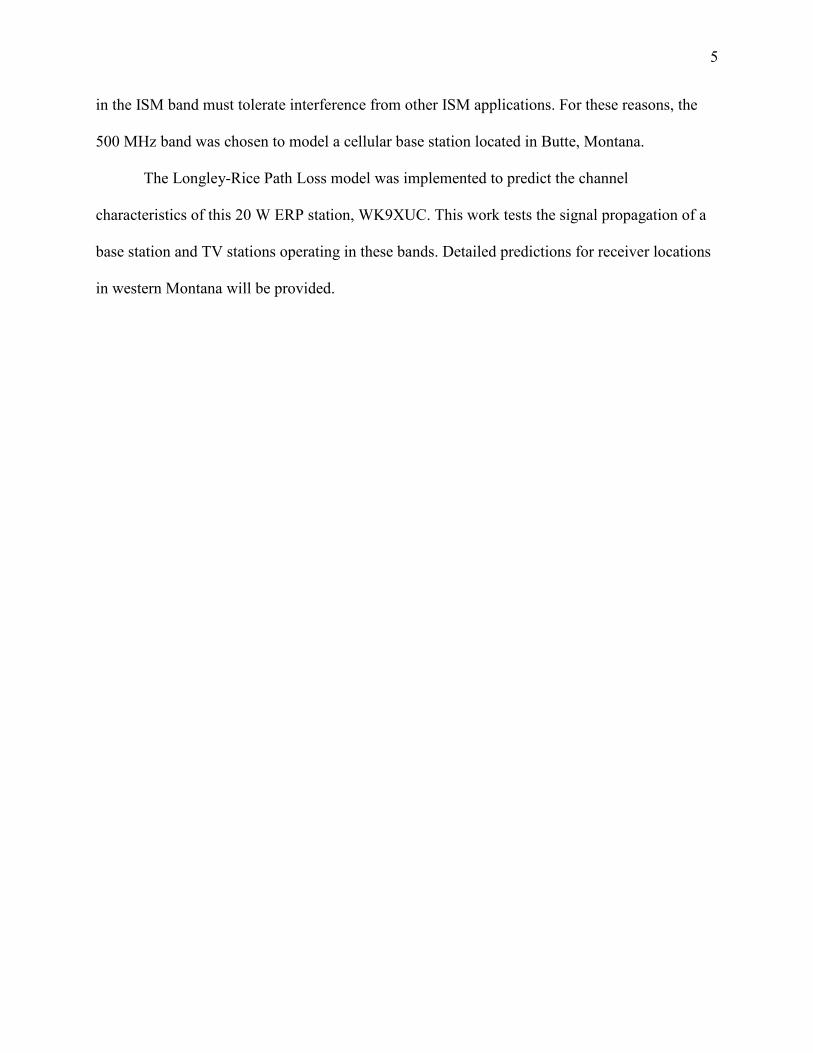
amount of time that users have cellular (specifically LTE) network access [38]. Figure 1 depicts

2G/3G and LTE (4G) coverage maps nationwide retrieved on the 1st of May 2017 [39].

Figure 1: Open Signal 2G/3G and LTE Coverage Map of USA

8

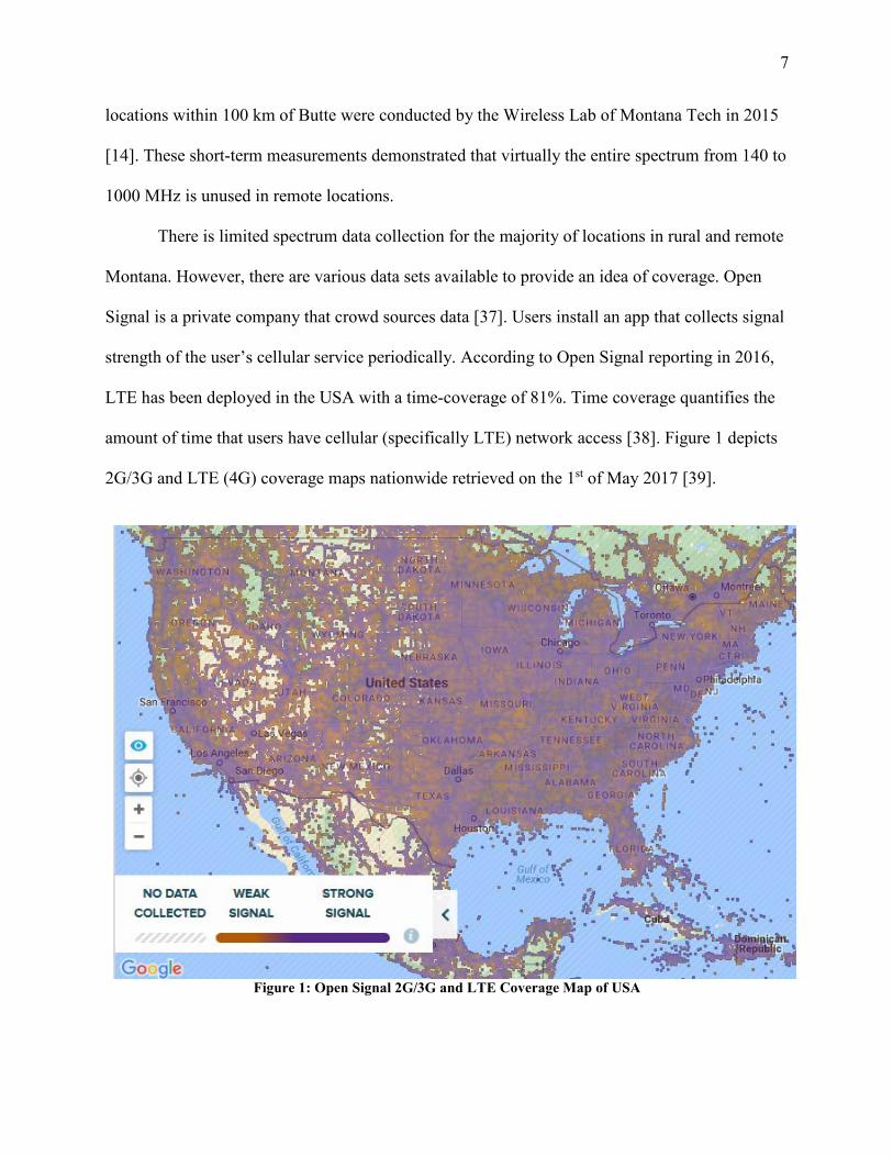
Figure 2 depicts a coverage map for the state of Montana.

Figure 2: Open Signal 2G/3G and LTE Coverage Map of Montana

Note that most test locations are located in and around population centers and along

highway and interstate systems. The majority of the state has no data collection as performed by

Open Signal. It is likely that a majority of the state of Montana has no meaningful coverage.

9

3. Technical Background

In modern communication systems any given channel will have a carrier frequency that is

modulated to convey information (data). A modulated carrier signal may have a time-varying

amplitude, frequency and/or phase:

𝑣𝑣(𝑡𝑡) = 𝐴𝐴(𝑡𝑡) cos(𝜔𝜔(𝑡𝑡)𝑡𝑡 + 𝜑𝜑(𝑡𝑡)) (1)

The baseband message (or data) is conveyed in the carrier signal by changing the

amplitude, frequency and/or phase of the carrier signal. This process is called modulation. At the

transmitter, a device called a mixer modulates a carrier signal, 𝑐𝑐(𝑡𝑡) with a baseband signal.

Although a mixer is a non-linear device, it is assumed that the mixer multiplies the baseband and

the carrier signal in Equation 2:

𝑣𝑣(𝑡𝑡) = 𝑐𝑐(𝑡𝑡) × 𝐴𝐴𝑏𝑏𝑏𝑏𝑏𝑏𝑏𝑏𝑏𝑏𝑏𝑏𝑏𝑏𝑏𝑏(𝑡𝑡)(cos 2𝜋𝜋𝑓𝑓𝑏𝑏𝑏𝑏𝑏𝑏𝑏𝑏𝑏𝑏𝑏𝑏𝑏𝑏𝑏𝑏 + 𝜙𝜙𝑏𝑏𝑏𝑏𝑏𝑏𝑏𝑏𝑏𝑏𝑏𝑏𝑏𝑏𝑏𝑏(𝑡𝑡)) (2)

The mixer that multiplies the two signals is called an upconverter because the modulated

signal has a higher frequency than the baseband signal (a downconverter would translate the

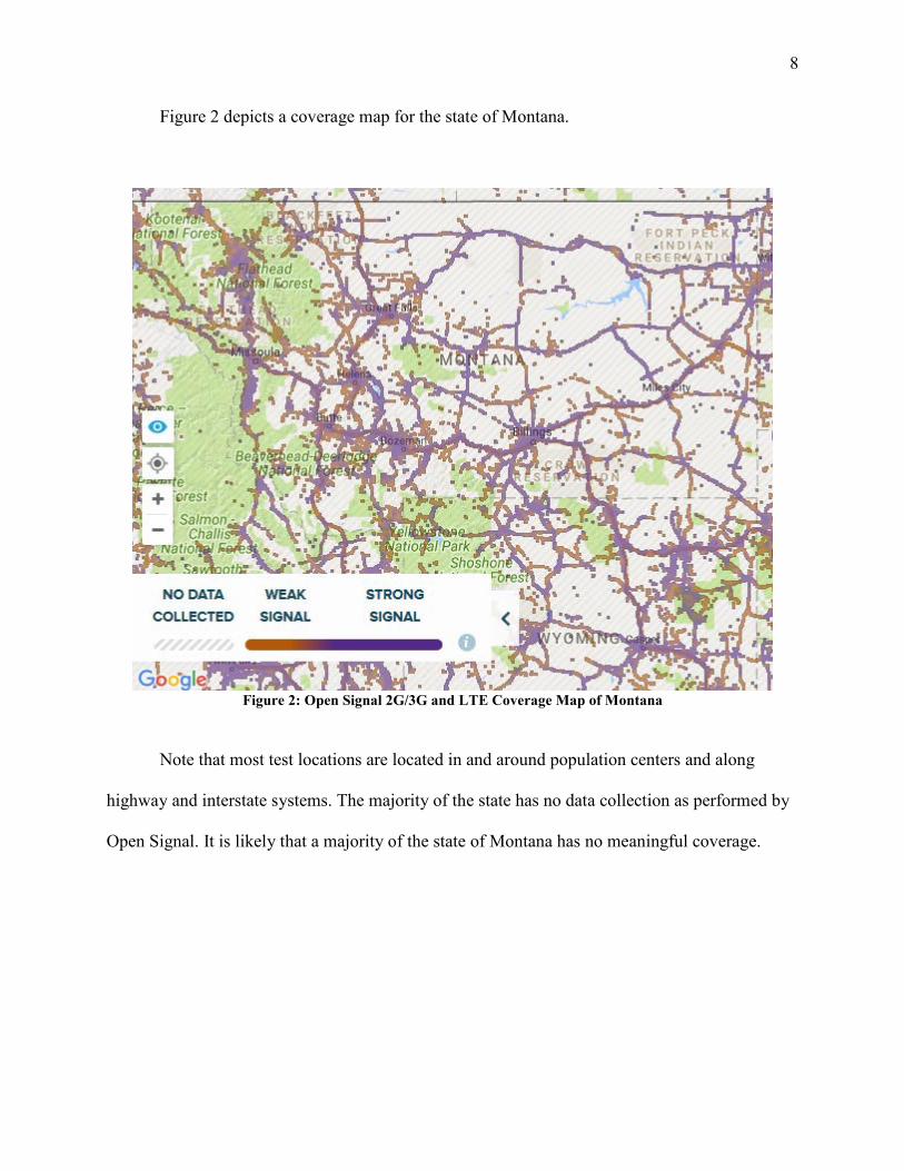
incoming signal to a lower frequency). A simplified diagram of modulation, called binary phase-

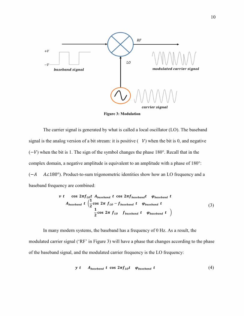
shift keying (BPSK) is pictured in Figure 3.

10

Figure 3: Modulation

The carrier signal is generated by what is called a local oscillator (LO). The baseband

signal is the analog version of a bit stream: it is positive (+𝑉𝑉) when the bit is 0, and negative

(−𝑉𝑉) when the bit is 1. The sign of the symbol changes the phase 180°. Recall that in the

complex domain, a negative amplitude is equivalent to an amplitude with a phase of 180°:

(−𝐴𝐴 = 𝐴𝐴∠180°). Product-to-sum trigonometric identities show how an LO frequency and a

baseband frequency are combined:

𝒗𝒗(𝒕𝒕) = 𝐜𝐜𝐜𝐜𝐜𝐜(𝟐𝟐𝟐𝟐𝟐𝟐𝑳𝑳𝑳𝑳𝒕𝒕)𝑨𝑨𝒃𝒃𝒃𝒃𝑵𝑵𝒃𝒃𝒃𝒃𝒃𝒃𝒃𝒃𝒃𝒃(𝒕𝒕) 𝐜𝐜𝐜𝐜𝐜𝐜(𝟐𝟐𝟐𝟐𝟐𝟐𝒃𝒃𝒃𝒃𝑵𝑵𝒃𝒃𝒃𝒃𝒃𝒃𝒃𝒃𝒃𝒃𝒕𝒕 + 𝝋𝝋𝒃𝒃𝒃𝒃𝑵𝑵𝒃𝒃𝒃𝒃𝒃𝒃𝒃𝒃𝒃𝒃(𝒕𝒕))

= 𝑨𝑨𝒃𝒃𝒃𝒃𝑵𝑵𝒃𝒃𝒃𝒃𝒃𝒃𝒃𝒃𝒃𝒃(𝒕𝒕) �𝟏𝟏𝟐𝟐𝐜𝐜𝐜𝐜𝐜𝐜(𝟐𝟐𝟐𝟐(𝟐𝟐𝑳𝑳𝑳𝑳 − 𝟐𝟐𝒃𝒃𝒃𝒃𝑵𝑵𝒃𝒃𝒃𝒃𝒃𝒃𝒃𝒃𝒃𝒃)𝒕𝒕 + 𝝋𝝋𝒃𝒃𝒃𝒃𝑵𝑵𝒃𝒃𝒃𝒃𝒃𝒃𝒃𝒃𝒃𝒃(𝒕𝒕))

+𝟏𝟏𝟐𝟐𝐜𝐜𝐜𝐜𝐜𝐜(𝟐𝟐𝟐𝟐(𝟐𝟐𝑳𝑳𝑳𝑳 + 𝟐𝟐𝒃𝒃𝒃𝒃𝑵𝑵𝒃𝒃𝒃𝒃𝒃𝒃𝒃𝒃𝒃𝒃)𝒕𝒕 + 𝝋𝝋𝒃𝒃𝒃𝒃𝑵𝑵𝒃𝒃𝒃𝒃𝒃𝒃𝒃𝒃𝒃𝒃(𝒕𝒕))�

(3)

In many modern systems, the baseband has a frequency of 0 Hz. As a result, the

modulated carrier signal (‘RF’ in Figure 3) will have a phase that changes according to the phase

of the baseband signal, and the modulated carrier frequency is the LO frequency:

𝒚𝒚(𝒕𝒕) = 𝑨𝑨𝒃𝒃𝒃𝒃𝑵𝑵𝒃𝒃𝒃𝒃𝒃𝒃𝒃𝒃𝒃𝒃(𝒕𝒕) 𝐜𝐜𝐜𝐜𝐜𝐜(𝟐𝟐𝟐𝟐𝟐𝟐𝑳𝑳𝑳𝑳𝒕𝒕 + 𝝋𝝋𝒃𝒃𝒃𝒃𝑵𝑵𝒃𝒃𝒃𝒃𝒃𝒃𝒃𝒃𝒃𝒃(𝒕𝒕)) (4)

11

A further consequence of sampling and filtering is that the modulated signal will occupy

a range of frequencies, known as the channel bandwidth (CBW):

𝟐𝟐𝒎𝒎𝒎𝒎𝒃𝒃𝒎𝒎𝒎𝒎𝒃𝒃𝒕𝒕𝒃𝒃𝒃𝒃 = 𝟐𝟐𝒄𝒄 ±𝟐𝟐𝒃𝒃𝒃𝒃𝒃𝒃𝒃𝒃𝒃𝒃𝒃𝒃𝒃𝒃𝒕𝒕𝒃𝒃

𝟐𝟐 (5)

In general, the spectrum allocation restricts the channel to a bandwidth. Filters are

implemented to adequately attenuate the sidebands. The bandwidth in turn limits the sampling

rate and data rate of channel communications.

The simplest way to model a communication channel is to perform propagation analysis

for a single link between a transmitter (Tx) and a receiver (Rx). A link budget is scaled in power

decibels and accounts for the power of the signal from the transmitter to the receiver, which

includes the transmit power, 𝑃𝑃𝑇𝑇𝑇𝑇, the gain or losses due to the Tx and Rx equipment, the path

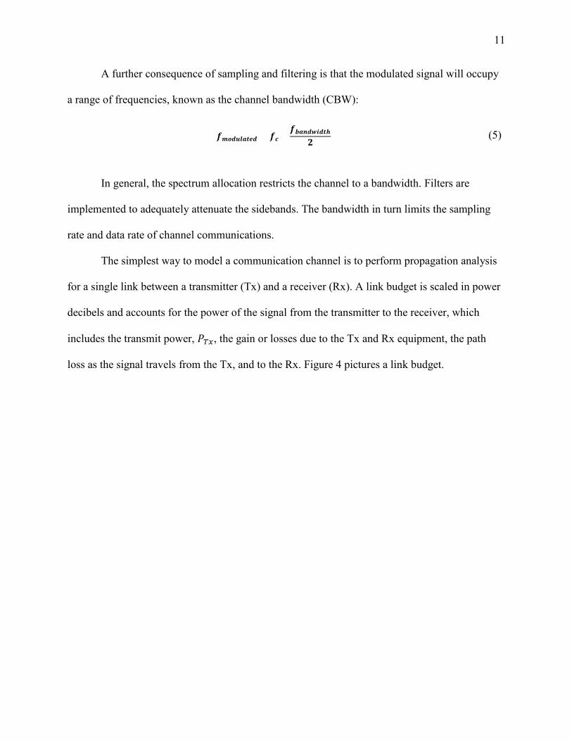
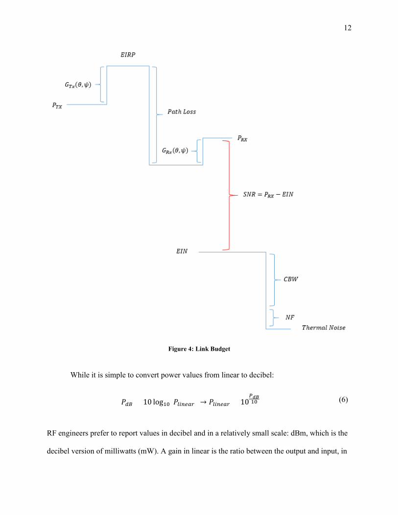
loss as the signal travels from the Tx, and to the Rx. Figure 4 pictures a link budget.

12

Figure 4: Link Budget

While it is simple to convert power values from linear to decibel:

𝑃𝑃𝑏𝑏𝑑𝑑 = 10 log10(𝑃𝑃𝑙𝑙𝑙𝑙𝑏𝑏𝑏𝑏𝑏𝑏𝑙𝑙) → 𝑃𝑃𝑙𝑙𝑙𝑙𝑏𝑏𝑏𝑏𝑏𝑏𝑙𝑙 = 10𝑃𝑃𝑑𝑑𝑑𝑑10 (6)

RF engineers prefer to report values in decibel and in a relatively small scale: dBm, which is the

decibel version of milliwatts (mW). A gain in linear is the ratio between the output and input, in

13

decibel this is the difference between the output and input and is reported in dB. However, dB

can also represent decibel watts, dBW (which is the decibel version of watt). Multiplication in

linear is equivalent to addition in logarithmic, similarly linear division is the same as logarithmic

subtraction. To convert from dBW to dBm simply add 30 dB:

𝑷𝑷𝒃𝒃𝒅𝒅𝒎𝒎 = 𝑷𝑷𝒃𝒃𝒅𝒅𝒅𝒅 + 𝟏𝟏𝟏𝟏 𝐥𝐥𝐜𝐜𝐥𝐥𝟏𝟏𝟏𝟏 �𝟏𝟏𝟏𝟏𝟏𝟏𝟏𝟏𝒎𝒎𝒅𝒅𝒅𝒅

� = 𝑷𝑷𝒃𝒃𝒅𝒅𝒅𝒅 + 𝟑𝟑𝟏𝟏 𝒃𝒃𝒅𝒅 (7)

The equivalent isotropic radiated power (EIRP) is the sum of the transmit power and the

gain of the Tx antenna. If the antenna has directivity, the relative position and orientation of the

antenna in relation to the Rx, will alter the gain (𝐺𝐺𝑇𝑇𝑇𝑇(𝜃𝜃,𝜓𝜓)) of the Tx antenna. Here 𝜃𝜃 represents

the elevation angle and 𝜓𝜓 represents the azimuth angle.

𝑬𝑬𝑬𝑬𝑬𝑬𝑷𝑷 = 𝑷𝑷𝑻𝑻𝑻𝑻 + 𝑮𝑮𝑻𝑻𝑻𝑻(𝜽𝜽,𝝍𝝍) (8)

Additionally, the Rx may employ equipment to increase its sensitivity. These include but

are not limited to the gain of the Rx antenna and of the amplifier. However, any loss due to

filters or attenuators decreases sensitivity. Therefore, the power at the receiver is the decibel sum

of EIRP, the path loss, and the losses or gains due Rx equipment:

𝑷𝑷𝑬𝑬𝑻𝑻 = 𝑬𝑬𝑬𝑬𝑬𝑬𝑷𝑷 + 𝑷𝑷𝒃𝒃𝒕𝒕𝒃𝒃 𝑳𝑳𝒎𝒎𝑵𝑵𝑵𝑵 − 𝑮𝑮𝑬𝑬𝑻𝑻(𝜽𝜽,𝝍𝝍) (9)

The link budget figure is a visualization of power level at the receiver and the receiver

sensitivity. The noise floor is a metric that describes the sensitivity of the receiver. It is the

minimal detectable power level of the receiver. For a transmitter location and receiver location,

engineers will determine the power of the received signal relative to noise floor. This is called

14

the signal to noise ratio (SNR), a useful metric that quantifies the quality of the received signal

for a given scenario:

𝑺𝑺𝑵𝑵𝑬𝑬𝒎𝒎𝒃𝒃𝒃𝒃𝒃𝒃𝒃𝒃𝒍𝒍 =𝑷𝑷𝑬𝑬𝑻𝑻𝑬𝑬𝑬𝑬𝑵𝑵

→ 𝑺𝑺𝑵𝑵𝑬𝑬𝒃𝒃𝒅𝒅 = 𝑷𝑷𝑬𝑬𝑻𝑻𝒃𝒃𝒅𝒅 − 𝑬𝑬𝑬𝑬𝑵𝑵𝒃𝒃𝒅𝒅 (10)

For modern communication systems the SNR will in part determine the data rate. In general, a

higher data rate requires a larger SNR.

The noise level depends on the environment for a given communication link, which

includes but is not limited to the thermal noise of the channel and the internal noise of the Rx

equipment. Thermal noise is the smallest amount of power that may exist in a given CBW.

Thermal noise is calculated using the temperature (in Kelvins) and Boltzmann’s constant,

𝑘𝑘𝑏𝑏 �𝐽𝐽𝐽𝐽𝐽𝐽𝑙𝑙𝑏𝑏𝑏𝑏𝐾𝐾𝑏𝑏𝑙𝑙𝐾𝐾𝑙𝑙𝑏𝑏

�, where the CBW is assumed to be 1 Hz wide:

𝑵𝑵𝒎𝒎𝒃𝒃𝑵𝑵𝒃𝒃𝒕𝒕𝒃𝒃𝒃𝒃𝒍𝒍𝒎𝒎𝒃𝒃𝒎𝒎 = 𝟏𝟏𝟏𝟏 𝐥𝐥𝐜𝐜𝐥𝐥𝟏𝟏𝟏𝟏(𝒌𝒌𝒃𝒃𝑻𝑻) (11)

The internal noise of the equipment or noise figure (NF) is particular to each piece of

equipment and must be measured. The channel bandwidth and NF will raise the noise floor

according to the following equation, this metric is called the equivalent input noise (EIN):

𝑬𝑬𝑬𝑬𝑵𝑵 = 𝑵𝑵𝒎𝒎𝒃𝒃𝑵𝑵𝒃𝒃𝒕𝒕𝒃𝒃𝒃𝒃𝒍𝒍𝒎𝒎𝒃𝒃𝒎𝒎 + 𝟏𝟏𝟏𝟏 𝐥𝐥𝐜𝐜𝐥𝐥𝟏𝟏𝟏𝟏(𝑪𝑪𝒅𝒅𝒅𝒅) + 𝑵𝑵𝑵𝑵 (12)

The PSD of thermal noise has a limit of -174 dBm/Hz, when calculated in dBm, and a

temperature of 300 K.

The gain of an antenna is a ratio relative to an isotropic antenna. An isotropic antenna has

a gain of 1 in linear or 0 dBi in decibel. By changing an antenna’s directivity, the gain is directed

15

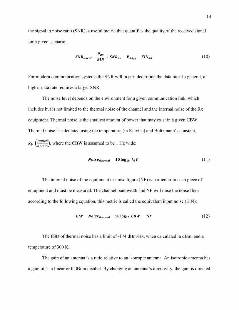
towards a point (or points) in space and away from others. Figure 5 depicts an omnidirectional

antenna in the azimuth direction that is shaped like a torus (donut). In contrast, an isotropic

antenna would be shaped like a sphere.

Figure 5: Antenna Pattern of Omnidirectional in Azimuth

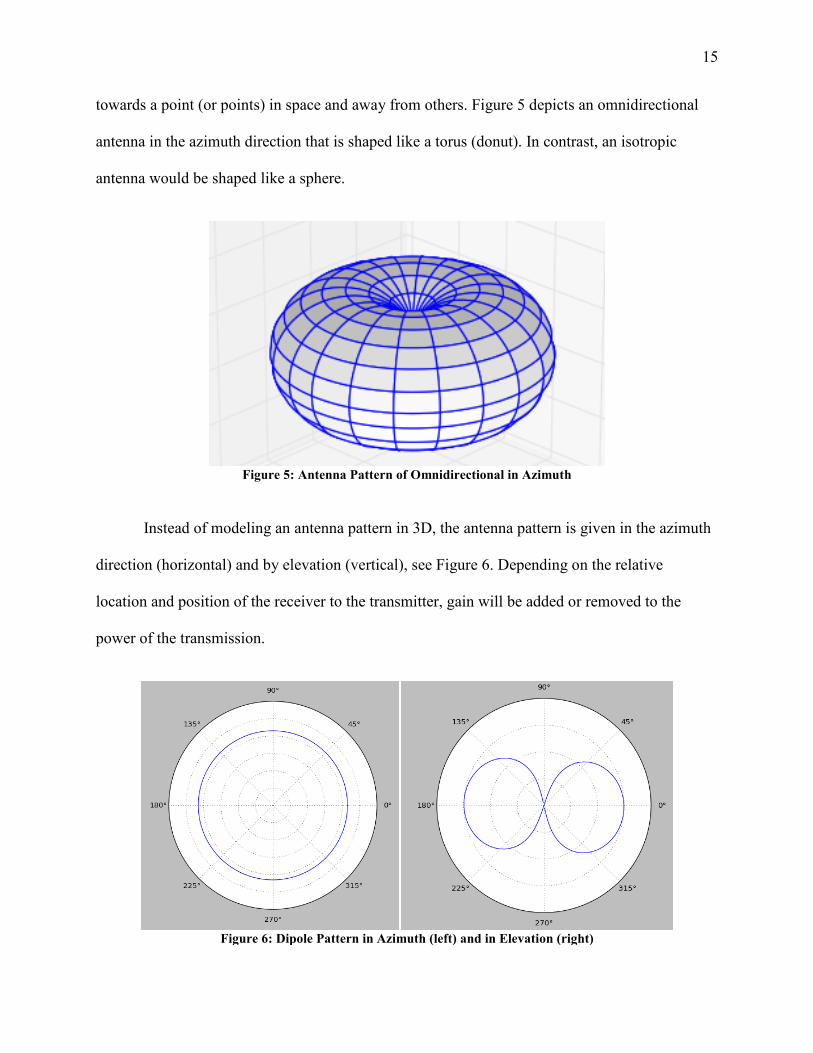
Instead of modeling an antenna pattern in 3D, the antenna pattern is given in the azimuth

direction (horizontal) and by elevation (vertical), see Figure 6. Depending on the relative

location and position of the receiver to the transmitter, gain will be added or removed to the

power of the transmission.

Figure 6: Dipole Pattern in Azimuth (left) and in Elevation (right)

16

When the direction of gain (either azimuth or elevation) is not given, the gain is understood to be

in the direction of the peak value, in which case the EIRP is a maximum.

𝑬𝑬𝑬𝑬𝑬𝑬𝑷𝑷𝒎𝒎𝒃𝒃𝑻𝑻 = 𝑷𝑷𝑻𝑻𝑻𝑻 + 𝑮𝑮𝑻𝑻𝑻𝑻,𝒎𝒎𝒃𝒃𝑻𝑻 (13)

The power for transmitter is generally restricted to a CBW. For the TV channels the

bandwidth is 6-MHz, and as discussed, the bandwidth of the target channels is 5-MHz.

Various models have been developed to model path loss for a given terrain and obstacles.

Some of these models will be described in more detail below. The most simple are theoretical

models operating in free-space (i.e. free of obstacles). A deterministic model would launch rays

from a Tx, and trace the rays as they interact with the environment. Various empirical models

have been developed by fitting collected data statistically. This work implements an empirical

model called the Longley-Rice Path Loss model, and its algorithm is called the Irregular Terrain

Model (ITM) [40].

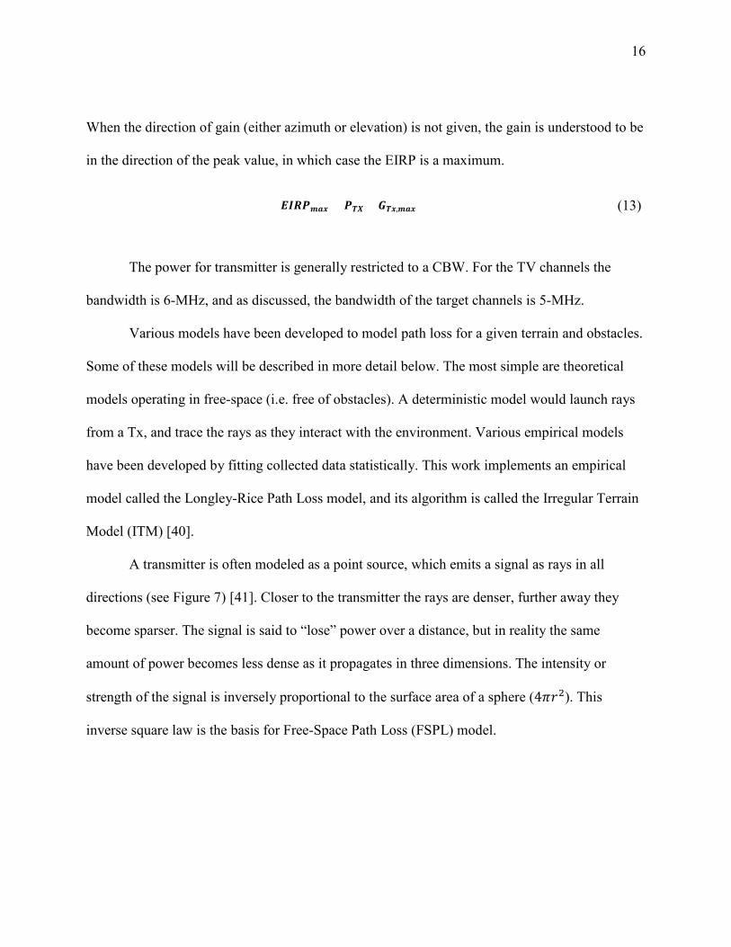
A transmitter is often modeled as a point source, which emits a signal as rays in all

directions (see Figure 7) [41]. Closer to the transmitter the rays are denser, further away they

become sparser. The signal is said to “lose” power over a distance, but in reality the same

amount of power becomes less dense as it propagates in three dimensions. The intensity or

strength of the signal is inversely proportional to the surface area of a sphere (4𝜋𝜋𝑟𝑟2). This

inverse square law is the basis for Free-Space Path Loss (FSPL) model.

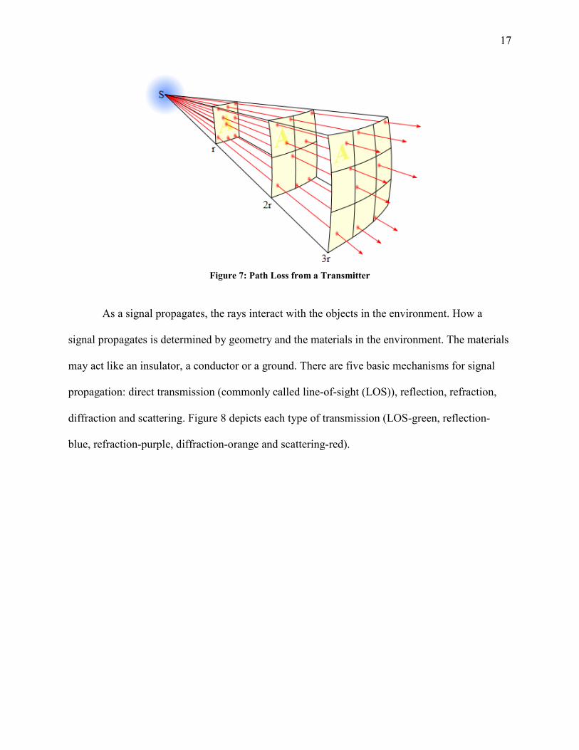
17

Figure 7: Path Loss from a Transmitter

As a signal propagates, the rays interact with the objects in the environment. How a

signal propagates is determined by geometry and the materials in the environment. The materials

may act like an insulator, a conductor or a ground. There are five basic mechanisms for signal

propagation: direct transmission (commonly called line-of-sight (LOS)), reflection, refraction,

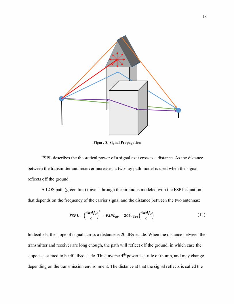
diffraction and scattering. Figure 8 depicts each type of transmission (LOS-green, reflection-

blue, refraction-purple, diffraction-orange and scattering-red).

18

Figure 8: Signal Propagation

FSPL describes the theoretical power of a signal as it crosses a distance. As the distance

between the transmitter and receiver increases, a two-ray path model is used when the signal

reflects off the ground.

A LOS path (green line) travels through the air and is modeled with the FSPL equation

that depends on the frequency of the carrier signal and the distance between the two antennas:

𝑵𝑵𝑺𝑺𝑷𝑷𝑳𝑳 = �𝟒𝟒𝟐𝟐𝒃𝒃𝟐𝟐𝒄𝒄𝒄𝒄

�𝟐𝟐

→ 𝑵𝑵𝑺𝑺𝑷𝑷𝑳𝑳𝒃𝒃𝒅𝒅 = 𝟐𝟐𝟏𝟏 𝐥𝐥𝐜𝐜𝐥𝐥𝟏𝟏𝟏𝟏 �𝟒𝟒𝟐𝟐𝒃𝒃𝟐𝟐𝒄𝒄𝒄𝒄

� (14)

In decibels, the slope of signal across a distance is 20 dB/decade. When the distance between the

transmitter and receiver are long enough, the path will reflect off the ground, in which case the

slope is assumed to be 40 dB/decade. This inverse 4th power is a rule of thumb, and may change

depending on the transmission environment. The distance at that the signal reflects is called the

19

cross-over (or critical) distance, 𝑑𝑑𝑐𝑐. This distance is determined by the height of the transmitter

antenna, ℎ𝑇𝑇𝑇𝑇 and the receiver antenna, ℎ𝑅𝑅𝑇𝑇 and the wavelength of the carrier signal:

𝒃𝒃𝒄𝒄 =𝟒𝟒𝟐𝟐𝒃𝒃𝒕𝒕𝑻𝑻𝒃𝒃𝒍𝒍𝑻𝑻

𝝀𝝀 (15)

Increasing the height of either antenna will increase this distance, and lowering the

frequency of the signal will decrease this distance. When the distance is greater than the cross-

over distance the path loss is proportional to an inverse 4th power of distance, ∝ 1𝑏𝑏4

:

𝑷𝑷𝒃𝒃𝒕𝒕𝒃𝒃 𝑳𝑳𝒎𝒎𝑵𝑵𝑵𝑵𝒈𝒈𝒍𝒍𝒎𝒎𝒎𝒎𝒃𝒃𝒃𝒃 𝒍𝒍𝒃𝒃𝟐𝟐𝒎𝒎𝒃𝒃𝒄𝒄𝒕𝒕𝒃𝒃𝒎𝒎𝒃𝒃 =𝒃𝒃𝒕𝒕𝑻𝑻𝟐𝟐 𝒃𝒃𝒍𝒍𝑻𝑻𝟐𝟐

𝒃𝒃𝟒𝟒

→ 𝑃𝑃𝑃𝑃𝑡𝑡ℎ 𝐿𝐿𝐿𝐿𝐿𝐿𝐿𝐿𝑔𝑔𝑙𝑙𝐽𝐽𝐽𝐽𝑏𝑏𝑏𝑏 𝑙𝑙𝑏𝑏𝑟𝑟𝑙𝑙𝑏𝑏𝑐𝑐𝑟𝑟𝑙𝑙𝐽𝐽𝑏𝑏𝑑𝑑𝑑𝑑 = 20 log10(ℎ𝑟𝑟𝑇𝑇ℎ𝑙𝑙𝑇𝑇) − 40 log10(𝑑𝑑) (16)

Reflection is not limited to the ground, it can also reflect off of obstacles like buildings

(blue line in Figure 8), in which case the path loss of each distance is summed.

A signal will also pass through a medium and refract (or change direction). Depending on

the thickness of the material or type of material, refraction will likely result in absorption, i.e. the

medium acts like a filter and dissipates the energy in the signal.

Diffraction, sometimes called knife-edge diffraction occurs when the signal is redirected

by well-defined obstacle, like the roof of a building. When the object is rounded, the rays will

diffract when the diameter of the object is larger than wavelength of the signal. Scattering occurs

when the shape of the material is much smaller in diameter than the wavelength of the signal.

This ITM model assumes that the LOS is the dominant-path and does not account for

multipath components directly. If there is an obstacle along the direct path, the algorithm

determines additional attenuation to the direct path based on terrain parameters and elevation. In

contrast, a ray-launching model would account for the multipath propagation but it requires

20

sufficient knowledge of the radio environment: location, geometry and material of the obstacles;

ultimately, a ray launching program requires greater computation time and larger memory needs

than a model like ITM.

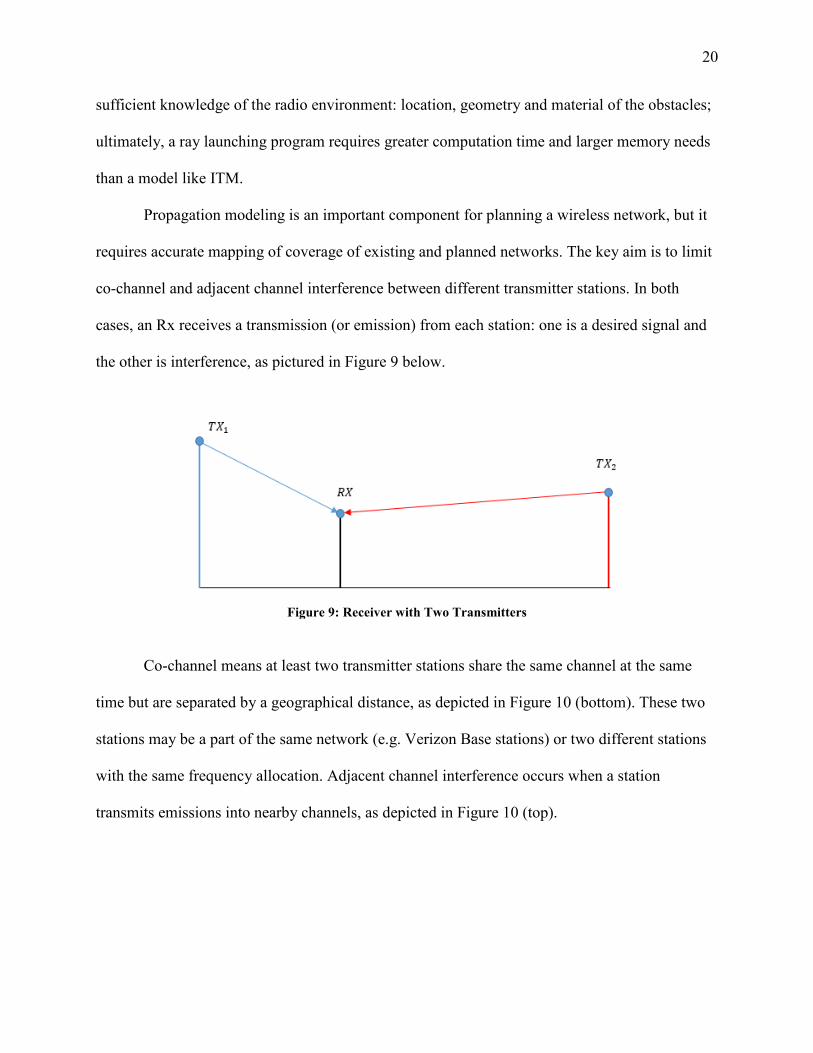
Propagation modeling is an important component for planning a wireless network, but it

requires accurate mapping of coverage of existing and planned networks. The key aim is to limit

co-channel and adjacent channel interference between different transmitter stations. In both

cases, an Rx receives a transmission (or emission) from each station: one is a desired signal and

the other is interference, as pictured in Figure 9 below.

Figure 9: Receiver with Two Transmitters

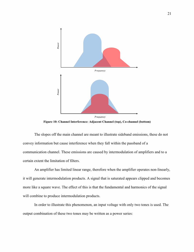
Co-channel means at least two transmitter stations share the same channel at the same

time but are separated by a geographical distance, as depicted in Figure 10 (bottom). These two

stations may be a part of the same network (e.g. Verizon Base stations) or two different stations

with the same frequency allocation. Adjacent channel interference occurs when a station

transmits emissions into nearby channels, as depicted in Figure 10 (top).

21

Figure 10: Channel Interference: Adjacent Channel (top), Co-channel (bottom)

The slopes off the main channel are meant to illustrate sideband emissions, these do not

convey information but cause interference when they fall within the passband of a

communication channel. These emissions are caused by intermodulation of amplifiers and to a

certain extent the limitation of filters.

An amplifier has limited linear range, therefore when the amplifier operates non-linearly,

it will generate intermodulation products. A signal that is saturated appears clipped and becomes

more like a square wave. The effect of this is that the fundamental and harmonics of the signal

will combine to produce intermodulation products.

In order to illustrate this phenomenon, an input voltage with only two tones is used. The

output combination of these two tones may be written as a power series:

22

𝒗𝒗𝒎𝒎𝒎𝒎𝒕𝒕 = 𝒌𝒌𝟏𝟏 + 𝒌𝒌𝟏𝟏𝒗𝒗𝒃𝒃𝒃𝒃 + 𝒌𝒌𝟐𝟐𝒗𝒗𝒃𝒃𝒃𝒃𝟐𝟐 + 𝒌𝒌𝟑𝟑𝒗𝒗𝒃𝒃𝒃𝒃𝟑𝟑 + ⋯ (17)

where,

𝒗𝒗𝒃𝒃𝒃𝒃 = 𝐜𝐜𝐜𝐜𝐜𝐜(𝝎𝝎𝟏𝟏𝒕𝒕) + 𝐜𝐜𝐜𝐜𝐜𝐜(𝝎𝝎𝟐𝟐𝒕𝒕) (18)

As a consequence, the frequencies present in the output signal are the sums and differences

between integer multiples of the two tones:

𝟐𝟐𝒎𝒎𝒎𝒎𝒕𝒕 = |𝒎𝒎𝟐𝟐𝟏𝟏 ± 𝒃𝒃𝟐𝟐𝟐𝟐| (19)

where m and n are integers that increment through the harmonics of each frequency. The signal

is filtered to remove (most) of these intermodulation artifacts. However, the 3rd order intermods

and 5th order intermods both fall within the passband of the channel:

Table I: Problematic Intermodulation Products Intermodulation Frequency

𝐼𝐼𝐼𝐼3 [2𝑓𝑓1 − 𝑓𝑓2 2𝑓𝑓2 − 𝑓𝑓1] 𝐼𝐼𝐼𝐼5 [3𝑓𝑓1 − 2𝑓𝑓2 3𝑓𝑓2 − 2𝑓𝑓1]

Depending on the degree of saturation, the channel power will be raised and potentially emit into

other channels and/or interfere with itself.

There are several metrics to characterize interference. One is the signal to interference

and noise ratio (SINR), it is similar to SNR, but the EIN and the power of the inference are

summed linearly:

𝑺𝑺𝑬𝑬𝑵𝑵𝑬𝑬𝒃𝒃𝒅𝒅 = 𝑷𝑷𝑬𝑬𝑻𝑻𝒃𝒃𝒅𝒅 − 𝟏𝟏𝟏𝟏 𝒎𝒎𝒎𝒎𝒈𝒈𝟏𝟏𝟏𝟏(𝑬𝑬𝑬𝑬𝑵𝑵𝒎𝒎𝒃𝒃𝒃𝒃𝒃𝒃𝒃𝒃𝒍𝒍 + 𝑷𝑷𝒃𝒃𝒃𝒃𝒕𝒕𝒃𝒃𝟐𝟐𝒃𝒃𝒍𝒍𝒃𝒃𝒃𝒃𝒄𝒄𝒃𝒃) (20)

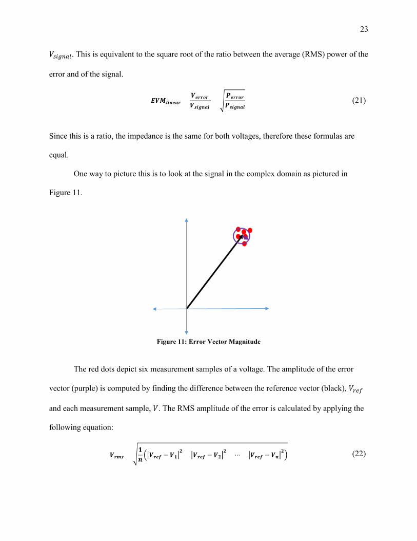
Another metric is the error vector magnitude (EVM). EVM is the ratio between the Root

Mean Square (RMS) amplitude of the error, 𝑉𝑉𝑏𝑏𝑙𝑙𝑙𝑙𝐽𝐽𝑙𝑙 and the RMS amplitude of the desired signal,

23

𝑉𝑉𝑏𝑏𝑙𝑙𝑔𝑔𝑏𝑏𝑏𝑏𝑙𝑙. This is equivalent to the square root of the ratio between the average (RMS) power of the

error and of the signal.

𝑬𝑬𝑬𝑬𝑴𝑴𝒎𝒎𝒃𝒃𝒃𝒃𝒃𝒃𝒃𝒃𝒍𝒍 =𝑬𝑬𝒃𝒃𝒍𝒍𝒍𝒍𝒎𝒎𝒍𝒍

𝑬𝑬𝑵𝑵𝒃𝒃𝒈𝒈𝒃𝒃𝒃𝒃𝒎𝒎 = �

𝑷𝑷𝒃𝒃𝒍𝒍𝒍𝒍𝒎𝒎𝒍𝒍𝑷𝑷𝑵𝑵𝒃𝒃𝒈𝒈𝒃𝒃𝒃𝒃𝒎𝒎

(21)

Since this is a ratio, the impedance is the same for both voltages, therefore these formulas are

equal.

One way to picture this is to look at the signal in the complex domain as pictured in

Figure 11.

Figure 11: Error Vector Magnitude

The red dots depict six measurement samples of a voltage. The amplitude of the error

vector (purple) is computed by finding the difference between the reference vector (black), 𝑉𝑉𝑙𝑙𝑏𝑏𝑟𝑟

and each measurement sample, 𝑉𝑉. The RMS amplitude of the error is calculated by applying the

following equation:

𝑬𝑬𝒍𝒍𝒎𝒎𝑵𝑵 = �𝟏𝟏𝒃𝒃��𝑬𝑬𝒍𝒍𝒃𝒃𝟐𝟐 − 𝑬𝑬𝟏𝟏�

𝟐𝟐 + �𝑬𝑬𝒍𝒍𝒃𝒃𝟐𝟐 − 𝑬𝑬𝟐𝟐�𝟐𝟐 + ⋯+ �𝑬𝑬𝒍𝒍𝒃𝒃𝟐𝟐 − 𝑬𝑬𝒃𝒃�

𝟐𝟐� (22)

24

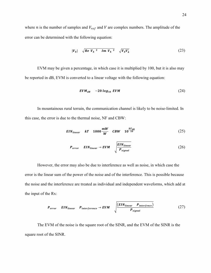
where 𝑛𝑛 is the number of samples and 𝑉𝑉𝑙𝑙𝑏𝑏𝑟𝑟 and 𝑉𝑉 are complex numbers. The amplitude of the

error can be determined with the following equation:

|𝑬𝑬𝒌𝒌| = �𝑬𝑬𝒃𝒃(𝑬𝑬𝒌𝒌)𝟐𝟐 + 𝑬𝑬𝒎𝒎(𝑬𝑬𝒌𝒌)𝟐𝟐 = �𝑬𝑬𝒌𝒌𝑬𝑬𝒌𝒌∗ (23)

EVM may be given a percentage, in which case it is multiplied by 100, but it is also may

be reported in dB, EVM is converted to a linear voltage with the following equation:

𝑬𝑬𝑬𝑬𝑴𝑴𝒃𝒃𝒅𝒅 = −𝟐𝟐𝟏𝟏 𝒎𝒎𝒎𝒎𝒈𝒈𝟏𝟏𝟏𝟏(𝑬𝑬𝑬𝑬𝑴𝑴) (24)

In mountainous rural terrain, the communication channel is likely to be noise-limited. In

this case, the error is due to the thermal noise, NF and CBW:

𝑬𝑬𝑬𝑬𝑵𝑵𝒎𝒎𝒃𝒃𝒃𝒃𝒃𝒃𝒃𝒃𝒍𝒍 = 𝒌𝒌𝑻𝑻 × 𝟏𝟏𝟏𝟏𝟏𝟏𝟏𝟏𝒎𝒎𝒅𝒅𝒅𝒅

× 𝑪𝑪𝒅𝒅𝒅𝒅 × 𝟏𝟏𝟏𝟏𝑵𝑵𝑵𝑵𝒃𝒃𝒅𝒅𝟏𝟏𝟏𝟏 (25)

𝑷𝑷𝒃𝒃𝒍𝒍𝒍𝒍𝒎𝒎𝒍𝒍 = 𝑬𝑬𝑬𝑬𝑵𝑵𝒎𝒎𝒃𝒃𝒃𝒃𝒃𝒃𝒃𝒃𝒍𝒍 → 𝑬𝑬𝑬𝑬𝑴𝑴 = �𝑬𝑬𝑬𝑬𝑵𝑵𝒎𝒎𝒃𝒃𝒃𝒃𝒃𝒃𝒃𝒃𝒍𝒍

𝑷𝑷𝑵𝑵𝒃𝒃𝒈𝒈𝒃𝒃𝒃𝒃𝒎𝒎 (26)

However, the error may also be due to interference as well as noise, in which case the

error is the linear sum of the power of the noise and of the interference. This is possible because

the noise and the interference are treated as individual and independent waveforms, which add at

the input of the Rx:

𝑷𝑷𝒃𝒃𝒍𝒍𝒍𝒍𝒎𝒎𝒍𝒍 = 𝑬𝑬𝑬𝑬𝑵𝑵𝒎𝒎𝒃𝒃𝒃𝒃𝒃𝒃𝒃𝒃𝒍𝒍 + 𝑷𝑷𝒃𝒃𝒃𝒃𝒕𝒕𝒃𝒃𝒍𝒍𝟐𝟐𝒃𝒃𝒍𝒍𝒃𝒃𝒃𝒃𝒄𝒄𝒃𝒃 → 𝑬𝑬𝑬𝑬𝑴𝑴 = ��𝑬𝑬𝑬𝑬𝑵𝑵𝒎𝒎𝒃𝒃𝒃𝒃𝒃𝒃𝒃𝒃𝒍𝒍 + 𝑷𝑷𝒃𝒃𝒃𝒃𝒕𝒕𝒃𝒃𝒍𝒍𝟐𝟐𝒃𝒃𝒃𝒃𝒄𝒄𝒃𝒃�

𝑷𝑷𝑵𝑵𝒃𝒃𝒈𝒈𝒃𝒃𝒃𝒃𝒎𝒎 (27)

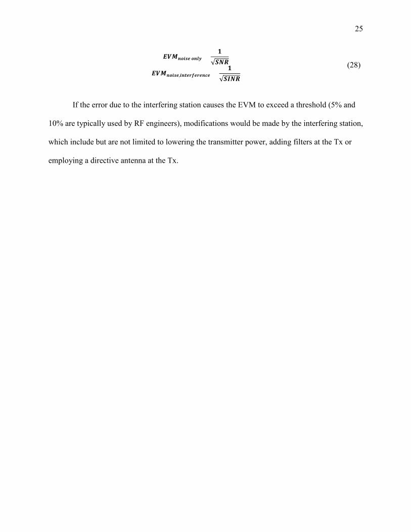
The EVM of the noise is the square root of the SINR, and the EVM of the SINR is the

square root of the SINR.

25

𝑬𝑬𝑬𝑬𝑴𝑴𝒃𝒃𝒎𝒎𝒃𝒃𝑵𝑵𝒃𝒃 𝒎𝒎𝒃𝒃𝒎𝒎𝒚𝒚 =𝟏𝟏

√𝑺𝑺𝑵𝑵𝑬𝑬

𝑬𝑬𝑬𝑬𝑴𝑴𝒃𝒃𝒎𝒎𝒃𝒃𝑵𝑵𝒃𝒃,𝒃𝒃𝒃𝒃𝒕𝒕𝒃𝒃𝒍𝒍𝟐𝟐𝒃𝒃𝒍𝒍𝒃𝒃𝒃𝒃𝒄𝒄𝒃𝒃 =𝟏𝟏

√𝑺𝑺𝑬𝑬𝑵𝑵𝑬𝑬

(28)

If the error due to the interfering station causes the EVM to exceed a threshold (5% and

10% are typically used by RF engineers), modifications would be made by the interfering station,

which include but are not limited to lowering the transmitter power, adding filters at the Tx or

employing a directive antenna at the Tx.

26

4. Spectrum Monitoring

4.1. Methodology

For this spectrum monitoring project, wireless communications are assessed by three

parameters: frequency, time and power. For the propagation modeling, space will be an added

parameter. This section provides technical information to explain how power measurements of

signals at different frequencies are collected over time. For this thesis work the frequency span of

interest is from 174 to 1000 MHz. The resolution bandwidth (RBW) is 488 kHz, resulting in

1692 frequency bins. This work collects the PSD dBm/Hz for each frequency bin.

The spectrum monitoring station, including the equipment and procedures at each

location will be described in detail. The spectrum monitoring station may be implemented as

either a fixed or mobile station; as such, this spectrum monitoring station may be adapted for

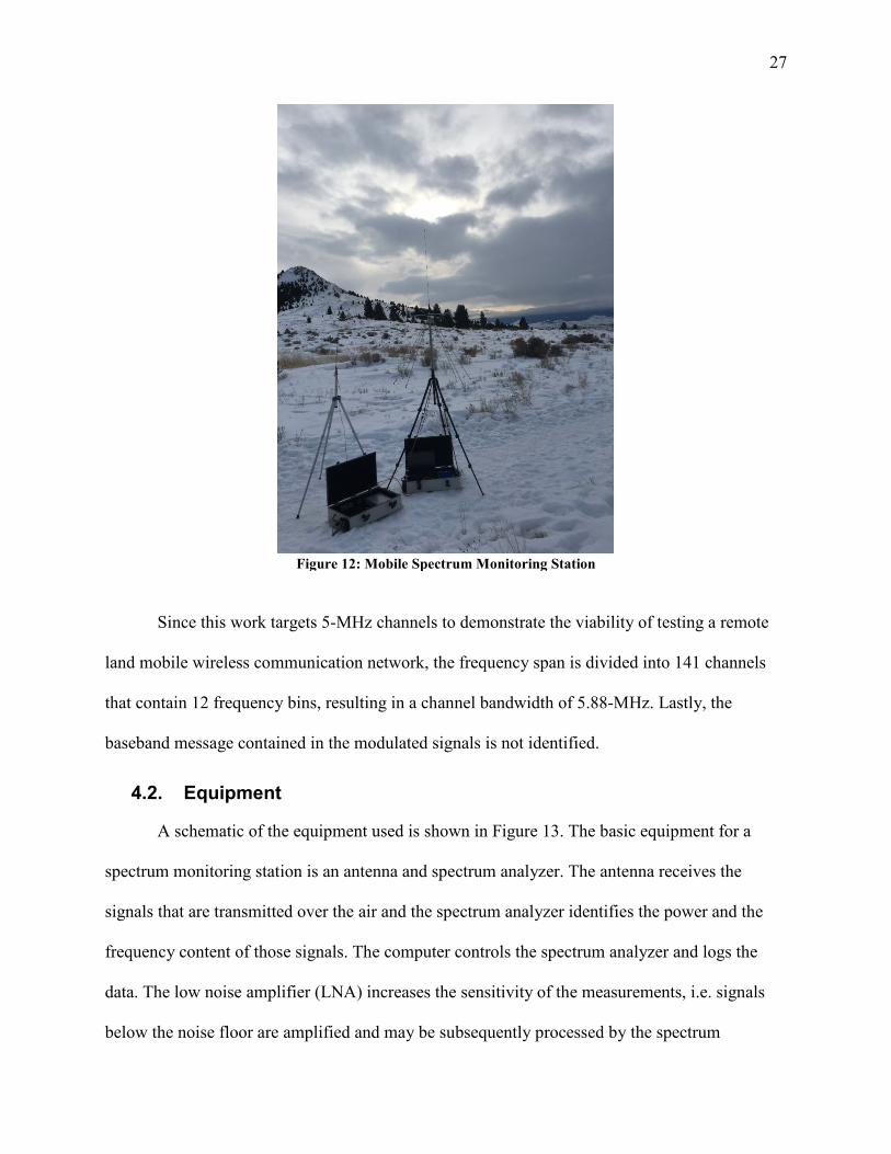
measurements in remote, rural and urban locations. Figure 12 pictures the mobile spectrum

monitoring station on site at a rural location.

27

Figure 12: Mobile Spectrum Monitoring Station

Since this work targets 5-MHz channels to demonstrate the viability of testing a remote

land mobile wireless communication network, the frequency span is divided into 141 channels

that contain 12 frequency bins, resulting in a channel bandwidth of 5.88-MHz. Lastly, the

baseband message contained in the modulated signals is not identified.

4.2. Equipment

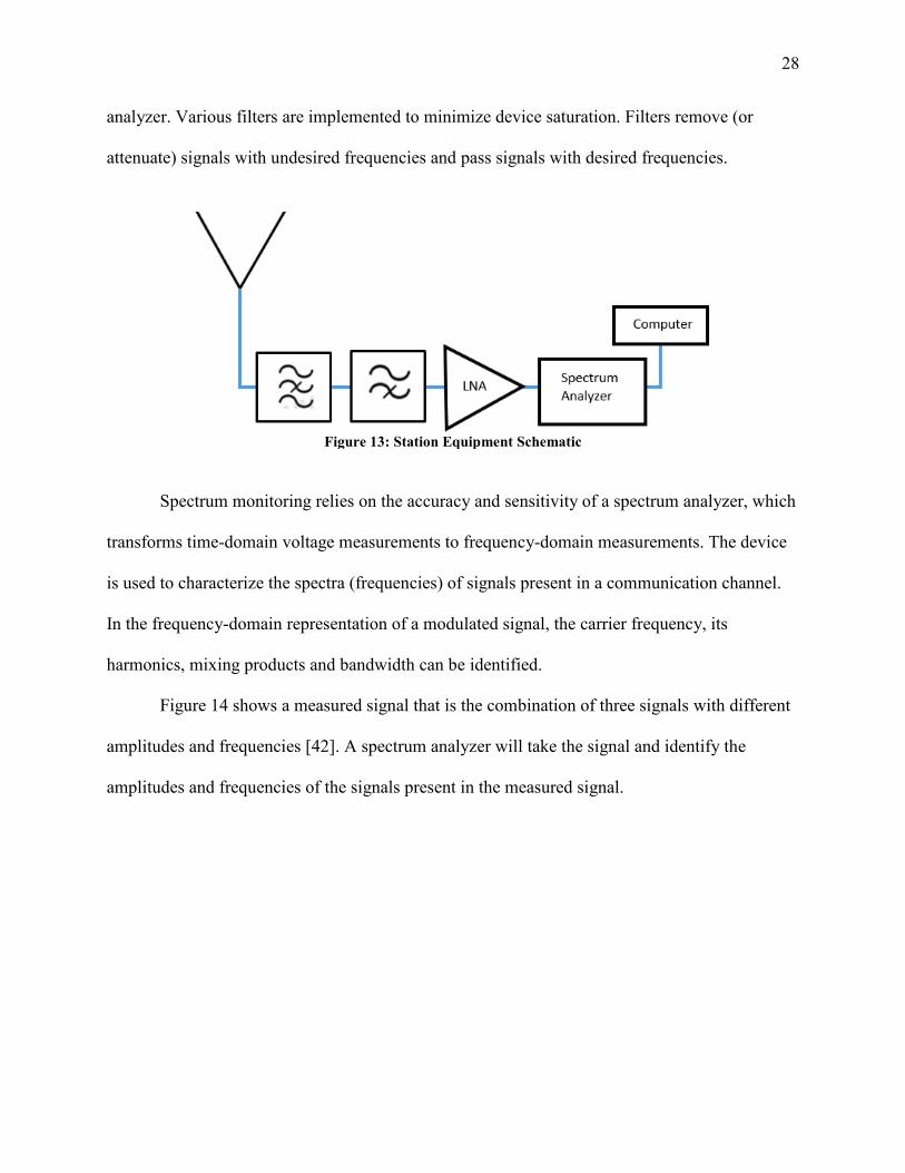
A schematic of the equipment used is shown in Figure 13. The basic equipment for a

spectrum monitoring station is an antenna and spectrum analyzer. The antenna receives the

signals that are transmitted over the air and the spectrum analyzer identifies the power and the

frequency content of those signals. The computer controls the spectrum analyzer and logs the

data. The low noise amplifier (LNA) increases the sensitivity of the measurements, i.e. signals

below the noise floor are amplified and may be subsequently processed by the spectrum

28

analyzer. Various filters are implemented to minimize device saturation. Filters remove (or

attenuate) signals with undesired frequencies and pass signals with desired frequencies.

Figure 13: Station Equipment Schematic

Spectrum monitoring relies on the accuracy and sensitivity of a spectrum analyzer, which

transforms time-domain voltage measurements to frequency-domain measurements. The device

is used to characterize the spectra (frequencies) of signals present in a communication channel.

In the frequency-domain representation of a modulated signal, the carrier frequency, its

harmonics, mixing products and bandwidth can be identified.

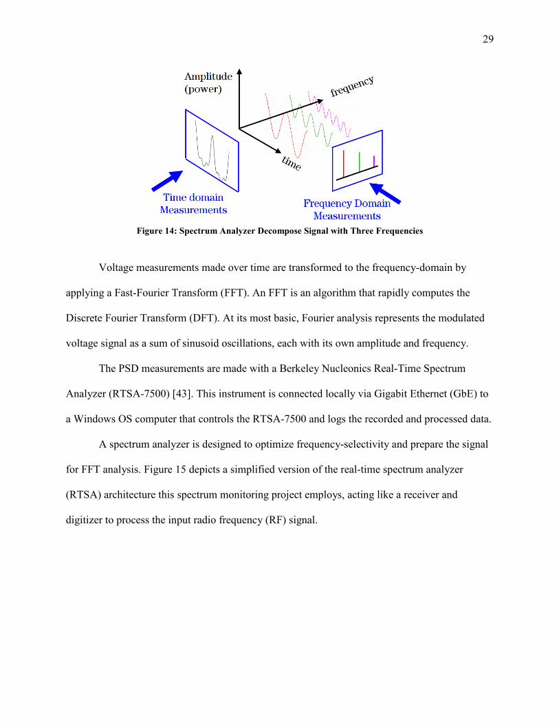
Figure 14 shows a measured signal that is the combination of three signals with different

amplitudes and frequencies [42]. A spectrum analyzer will take the signal and identify the

amplitudes and frequencies of the signals present in the measured signal.

29

Figure 14: Spectrum Analyzer Decompose Signal with Three Frequencies

Voltage measurements made over time are transformed to the frequency-domain by

applying a Fast-Fourier Transform (FFT). An FFT is an algorithm that rapidly computes the

Discrete Fourier Transform (DFT). At its most basic, Fourier analysis represents the modulated

voltage signal as a sum of sinusoid oscillations, each with its own amplitude and frequency.

The PSD measurements are made with a Berkeley Nucleonics Real-Time Spectrum

Analyzer (RTSA-7500) [43]. This instrument is connected locally via Gigabit Ethernet (GbE) to

a Windows OS computer that controls the RTSA-7500 and logs the recorded and processed data.

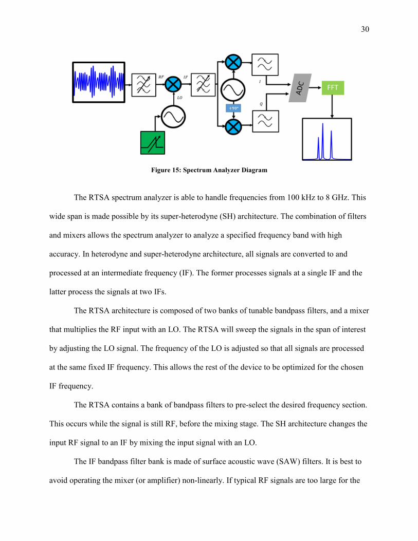
A spectrum analyzer is designed to optimize frequency-selectivity and prepare the signal

for FFT analysis. Figure 15 depicts a simplified version of the real-time spectrum analyzer

(RTSA) architecture this spectrum monitoring project employs, acting like a receiver and

digitizer to process the input radio frequency (RF) signal.

30

Figure 15: Spectrum Analyzer Diagram

The RTSA spectrum analyzer is able to handle frequencies from 100 kHz to 8 GHz. This

wide span is made possible by its super-heterodyne (SH) architecture. The combination of filters

and mixers allows the spectrum analyzer to analyze a specified frequency band with high

accuracy. In heterodyne and super-heterodyne architecture, all signals are converted to and

processed at an intermediate frequency (IF). The former processes signals at a single IF and the

latter process the signals at two IFs.

The RTSA architecture is composed of two banks of tunable bandpass filters, and a mixer

that multiplies the RF input with an LO. The RTSA will sweep the signals in the span of interest

by adjusting the LO signal. The frequency of the LO is adjusted so that all signals are processed

at the same fixed IF frequency. This allows the rest of the device to be optimized for the chosen

IF frequency.

The RTSA contains a bank of bandpass filters to pre-select the desired frequency section.

This occurs while the signal is still RF, before the mixing stage. The SH architecture changes the

input RF signal to an IF by mixing the input signal with an LO.

The IF bandpass filter bank is made of surface acoustic wave (SAW) filters. It is best to

avoid operating the mixer (or amplifier) non-linearly. If typical RF signals are too large for the

31

mixer, the operator would reduce the amplitude of the RF signal by lowering the gain of the

internal or external amplifier and/or adding appropriate attenuators and filters.

After the first mixing stage the IF has either a higher or a lower frequency than the input

RF signal, meaning it either up- or down-converted. For the frequency span of interest (174 to

1000 MHz), the frequencies are likely upconverted because the span of interest is on the lower

end of frequencies that the RTSA is able to process.

The next stage is called demodulation because it isolates the baseband by undoing the

modulation performed by the transmitter. RF engineers refer to the real part of the signal as I (for

in-phase), and the imaginary part is Q (for quadrature). The real and imaginary parts of the signal

are found by mixing the IF signal with another LO signal, 𝐿𝐿𝐿𝐿2. The real part is found by

multiplying the signal by a cosine, cos(2𝜋𝜋𝑓𝑓𝐿𝐿𝐿𝐿2). The LO signal is shifted in phase by 90°,

sin (2𝜋𝜋𝑓𝑓𝐿𝐿𝐿𝐿2) to find the imaginary component of the signal.

The 2nd oscillator frequency is fixed to be equal to the 1st IF frequency, 𝑓𝑓𝐿𝐿𝐿𝐿2 = 𝑓𝑓𝐼𝐼𝐼𝐼1

𝟐𝟐𝑬𝑬𝑵𝑵𝟐𝟐 = 𝟐𝟐𝑬𝑬𝑵𝑵𝟏𝟏 ± 𝟐𝟐𝑳𝑳𝑳𝑳𝟐𝟐 → [𝟏𝟏 𝑯𝑯𝑯𝑯 𝟐𝟐𝟐𝟐𝑬𝑬𝑵𝑵𝟏𝟏] (29)

Therefore, the output signal of this mixing stage has frequencies at baseband (0 Hz) and

double the IF frequency, the latter of which are removed with a low pass filter. Gain and phase

correction are also be applied after filtering. The outputs of this stage are analog in-phase

quadrature (IQ) signals.

(Note a simplified version of the RTSA is pictured as heterodyne in Figure 15 above. In

SH mode, the RTSA will translate frequency into another IF and perform baseband

demodulation in the digital-domain not the analog-domain.)

32

As a result of multiple stages of filters the signal is said to be bandlimited, i.e. most of the

harmonics are removed and the communication link is restricted to the bandwidth of the

baseband message. Presenting the signals as IQ measurements is a handy way to retain the phase

information of the signals. It also makes the subsequent calculations easier to perform, since

complex numbers are stored and evaluated in Cartesian form on computers.

Next, the analog signals are transformed into digital signals with the analog to digital

converter (ADC). The analog signal is sampled at 125 Msamples/sec. This stage prepares the

data for the FFT analysis. The signals must be discrete, the number of samples must be a power

of 2, and frequencies must represent data contained in (i.e. the baseband of) the input RF signal.

Depending on the RBW, the sampling frequency may be decreased after the ADC stage.

This process is called decimation because the signal sample is reduced in size. The data is often

processed by windowing to give a better estimate of the PSD. For windowing, the data is

separated into overlapping segments and the FFT is performed on each “window.” The

overlapping segments are then averaged to estimate the power present in each frequency bin. A

common algorithm used to estimate the power is Welch’s method.

The program that controls the RTSA employs a built-in FFT from the NumPy module,

which is in widespread use [44]. The FFT result for each frequency bin, 𝑉𝑉𝑘𝑘, are conveyed as

power measurements by squaring the magnitude. Since the difference between each frequency

bin is the RBW, the PSD results are commonly returned with units of �𝑚𝑚𝑚𝑚𝑅𝑅𝑑𝑑𝑚𝑚

� or �𝑏𝑏𝑑𝑑𝑚𝑚𝑅𝑅𝑑𝑑𝑚𝑚

�:

𝑷𝑷𝑺𝑺𝑫𝑫𝒌𝒌 �𝒎𝒎𝒅𝒅𝑬𝑬𝒅𝒅𝒅𝒅

� =|𝑬𝑬𝒌𝒌|𝟐𝟐

𝒁𝒁→ 𝟐𝟐𝟏𝟏 𝐥𝐥𝐜𝐜𝐥𝐥𝟏𝟏𝟏𝟏(|𝑬𝑬𝒌𝒌|) − 𝟏𝟏𝟏𝟏 𝐥𝐥𝐜𝐜𝐥𝐥𝟏𝟏𝟏𝟏(𝒁𝒁) �

𝒃𝒃𝒅𝒅𝒎𝒎𝑬𝑬𝒅𝒅𝒅𝒅

� (30)

In practice, RF equipment is calibrated to have an impedance match, 50 Ω. When each

piece of equipment has the same impedance, the equivalent impedance on either the input or the

33

output of each device looks like a 50Ω load. This station implements 50Ω impedance. Impedance

matching enables the maximum amount of power to be transferred from each piece of equipment

to the other and limits the reflections that travel back from either port. The equipment for RF has

a standard impedance match of 50 Ω, however when converted from analog to digital the

impedance is likely larger (around 1 kΩ).

Now, the rest of the station equipment will be described in greater detail. At either a fixed

or mobile station, the reference antenna is a Diamond D3000N Super Discone with a nominal

gain of 2 dBi [45]. The D3000N is a wideband omnidirectional (in azimuth) antenna capable of

receiving signals from 25 to 3000 MHz. The D3000N is mounted vertically at each location;

therefore the antenna is most sensitive to signals that travel along the horizon.

An LNA is employed at both the fixed and mobile stations. An LNA improves the

sensitivity of the measurements by amplifying the received signals while adding minimal noise.

At a fixed location the RF Bay Inc. LNA-1520 amplifies the received signals by 20.1 ± 0.60 dB

[46]. In mobile locations, the COM Power PAM-103 amplifies the received signals by 35.5 ±

0.80 dB [47]. The fixed location receives higher-powered signals that require a smaller gain to

avoid saturation.

Depending on the location, either the LNA or RTSA-7500 spectrum analyzer is prone to

saturation due to FM signals or 2-way hand held radios between 150 and 165 MHz. The FM

radio station at Montana Tech, KMSM (103.9), is a particular nuisance; it is possible to

demodulate and listen to the musical programming being transmitted on the station’s 3rd

harmonic. Since these bands are not of interest, a high pass filter is employed before the LNA.

The HP 7162/174 S50 filter from Tin Lee Electronics provides minimum attenuation (-0.74 ±

34

0.52 dB) along the span of interest and attenuates signals below 164 MHz by at least 40 dB and

up to 101 dB [48].

There are several power limiting measures employed to prevent damage to the front-end

of the LNA and the RTSA-7500. The first, an L-com Coaxial Lighting Protector AL-NMNFB

contains a gas-discharge tube that acts as a fuse [49]. When the gas burns, the energy is directed

towards earth ground. The surge protector is connected to earth ground via the power breaker

box located in the room. For this reason, it is only employed at the fixed Museum station.

Furthermore, it is placed between the antenna and the filters.

The second power limiting measure is a modified FM Notch filter FLT201A/N from

Stridsberg Engineering [50]. A 10 kΩ surface mount resistor was soldered between the center

feedline and ground that is normally open. This “bleeder” resistor dissipates the static electricity

that accumulates along the co-axial cable and antenna as they move. This modification moved

the notch slightly; the filter attenuates the received signals by -35.5 dB and -32.5 dB at 88 MHz

and 108 MHz respectively.

Third, the LNA acts as a power-limiting device. P1dB is a metric used to quantify the

saturation point of the amplifier. It is assumed that the P1dB is near the maximum power output

from the LNA. To locate the P1dB point, one needs to determine the slope of the transmitter

when it operates linearly, then find the difference of 1 dB between the slope and the output gain

measurements. If the P1dB of the LNA is greater than +10dBm, which is the maximum RF Input

at the RTSA-7500, the appropriately-sized attenuator is put inline between the two.

Additional attenuators may be required if the signals present at a given location cause

device saturation. External batteries power all equipment for the mobile station, while AC/DC

power adapters power devices at locations with available power. DC blocks are placed before the

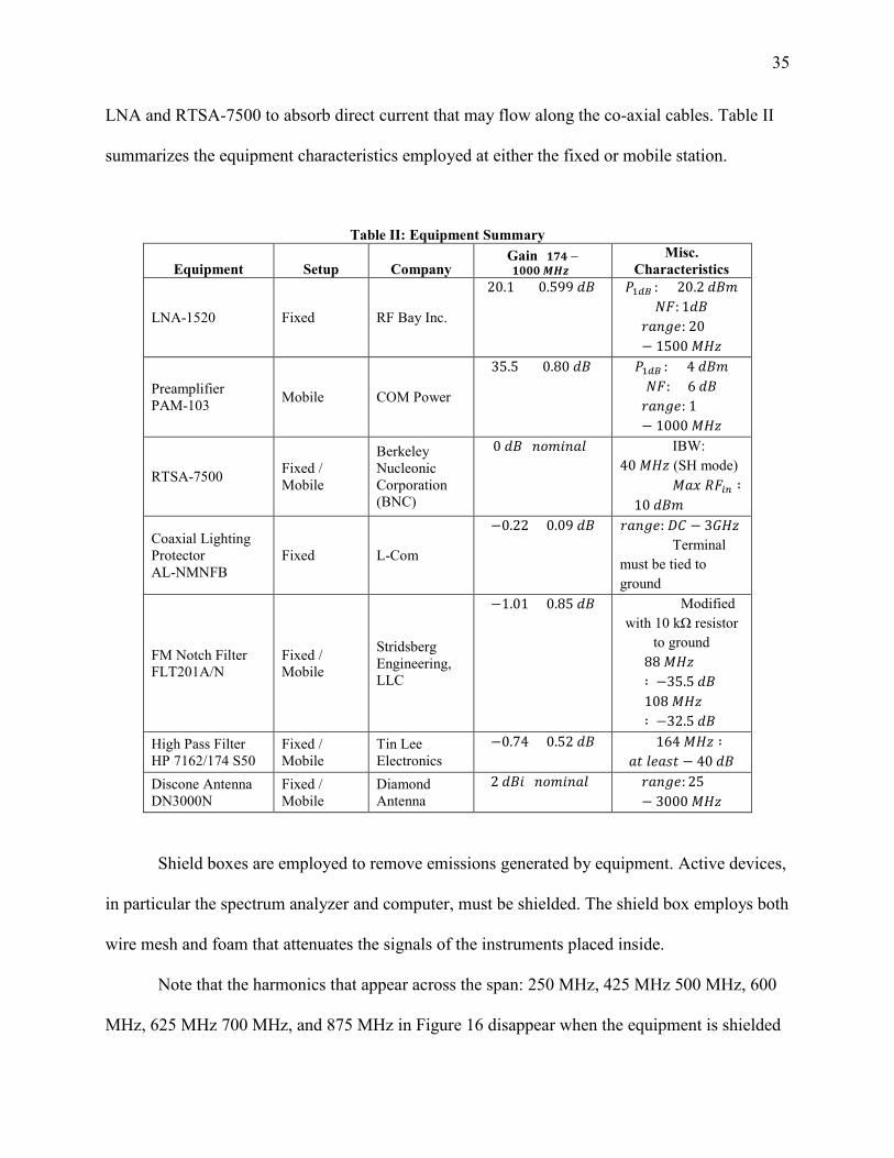
35

LNA and RTSA-7500 to absorb direct current that may flow along the co-axial cables. Table II

summarizes the equipment characteristics employed at either the fixed or mobile station.

Table II: Equipment Summary

Equipment Setup Company Gain (𝟏𝟏𝟏𝟏𝟒𝟒 −𝟏𝟏𝟏𝟏𝟏𝟏𝟏𝟏 𝑴𝑴𝑯𝑯𝑯𝑯)

Misc. Characteristics

LNA-1520 Fixed RF Bay Inc.

20.1 ± 0.599 𝑑𝑑𝑑𝑑 𝑃𝑃1𝑏𝑏𝑑𝑑 : + 20.2 𝑑𝑑𝑑𝑑𝑑𝑑 𝑁𝑁𝑁𝑁: 1𝑑𝑑𝑑𝑑

𝑟𝑟𝑃𝑃𝑛𝑛𝑟𝑟𝑟𝑟: 20− 1500 𝐼𝐼𝑀𝑀𝑀𝑀

Preamplifier PAM-103 Mobile COM Power

35.5 ± 0.80 𝑑𝑑𝑑𝑑 𝑃𝑃1𝑏𝑏𝑑𝑑 : + 4 𝑑𝑑𝑑𝑑𝑑𝑑 𝑁𝑁𝑁𝑁: < 6 𝑑𝑑𝑑𝑑 𝑟𝑟𝑃𝑃𝑛𝑛𝑟𝑟𝑟𝑟: 1− 1000 𝐼𝐼𝑀𝑀𝑀𝑀

RTSA-7500 Fixed / Mobile

Berkeley Nucleonic Corporation (BNC)

0 𝑑𝑑𝑑𝑑 (𝑛𝑛𝐿𝐿𝑑𝑑𝑛𝑛𝑛𝑛𝑃𝑃𝑛𝑛) IBW: 40 𝐼𝐼𝑀𝑀𝑀𝑀 (SH mode)

𝐼𝐼𝑃𝑃𝑀𝑀 𝑅𝑅𝑁𝑁𝑙𝑙𝑏𝑏 ∶ +10 𝑑𝑑𝑑𝑑𝑑𝑑

Coaxial Lighting Protector AL-NMNFB

Fixed L-Com

−0.22 ± 0.09 𝑑𝑑𝑑𝑑 𝑟𝑟𝑃𝑃𝑛𝑛𝑟𝑟𝑟𝑟: 𝐷𝐷𝐷𝐷 − 3𝐺𝐺𝑀𝑀𝑀𝑀 Terminal

must be tied to ground

FM Notch Filter FLT201A/N

Fixed / Mobile

Stridsberg Engineering, LLC

−1.01 ± 0.85 𝑑𝑑𝑑𝑑 Modified with 10 kΩ resistor

to ground 88 𝐼𝐼𝑀𝑀𝑀𝑀∶ −35.5 𝑑𝑑𝑑𝑑 108 𝐼𝐼𝑀𝑀𝑀𝑀∶ −32.5 𝑑𝑑𝑑𝑑

High Pass Filter HP 7162/174 S50

Fixed / Mobile

Tin Lee Electronics

−0.74 ± 0.52 𝑑𝑑𝑑𝑑 < 164 𝐼𝐼𝑀𝑀𝑀𝑀 ∶ 𝑃𝑃𝑡𝑡 𝑛𝑛𝑟𝑟𝑃𝑃𝐿𝐿𝑡𝑡 − 40 𝑑𝑑𝑑𝑑

Discone Antenna DN3000N

Fixed / Mobile

Diamond Antenna

2 𝑑𝑑𝑑𝑑𝑛𝑛 (𝑛𝑛𝐿𝐿𝑑𝑑𝑛𝑛𝑛𝑛𝑃𝑃𝑛𝑛) 𝑟𝑟𝑃𝑃𝑛𝑛𝑟𝑟𝑟𝑟: 25− 3000 𝐼𝐼𝑀𝑀𝑀𝑀

Shield boxes are employed to remove emissions generated by equipment. Active devices,

in particular the spectrum analyzer and computer, must be shielded. The shield box employs both

wire mesh and foam that attenuates the signals of the instruments placed inside.

Note that the harmonics that appear across the span: 250 MHz, 425 MHz 500 MHz, 600

MHz, 625 MHz 700 MHz, and 875 MHz in Figure 16 disappear when the equipment is shielded

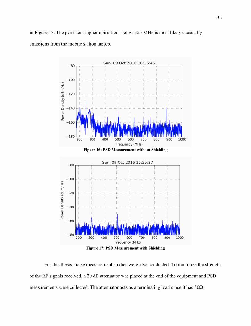
36

in Figure 17. The persistent higher noise floor below 325 MHz is most likely caused by

emissions from the mobile station laptop.

Figure 16: PSD Measurement without Shielding

Figure 17: PSD Measurement with Shielding

For this thesis, noise measurement studies were also conducted. To minimize the strength

of the RF signals received, a 20 dB attenuator was placed at the end of the equipment and PSD

measurements were collected. The attenuator acts as a terminating load since it has 50Ω

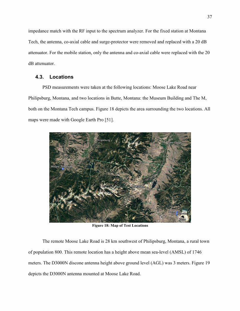
37

impedance match with the RF input to the spectrum analyzer. For the fixed station at Montana

Tech, the antenna, co-axial cable and surge-protector were removed and replaced with a 20 dB

attenuator. For the mobile station, only the antenna and co-axial cable were replaced with the 20

dB attenuator.

4.3. Locations

PSD measurements were taken at the following locations: Moose Lake Road near

Philipsburg, Montana, and two locations in Butte, Montana: the Museum Building and The M,

both on the Montana Tech campus. Figure 18 depicts the area surrounding the two locations. All

maps were made with Google Earth Pro [51].

Figure 18: Map of Test Locations

The remote Moose Lake Road is 28 km southwest of Philipsburg, Montana, a rural town

of population 800. This remote location has a height above mean sea-level (AMSL) of 1746

meters. The D3000N discone antenna height above ground level (AGL) was 3 meters. Figure 19

depicts the D3000N antenna mounted at Moose Lake Road.

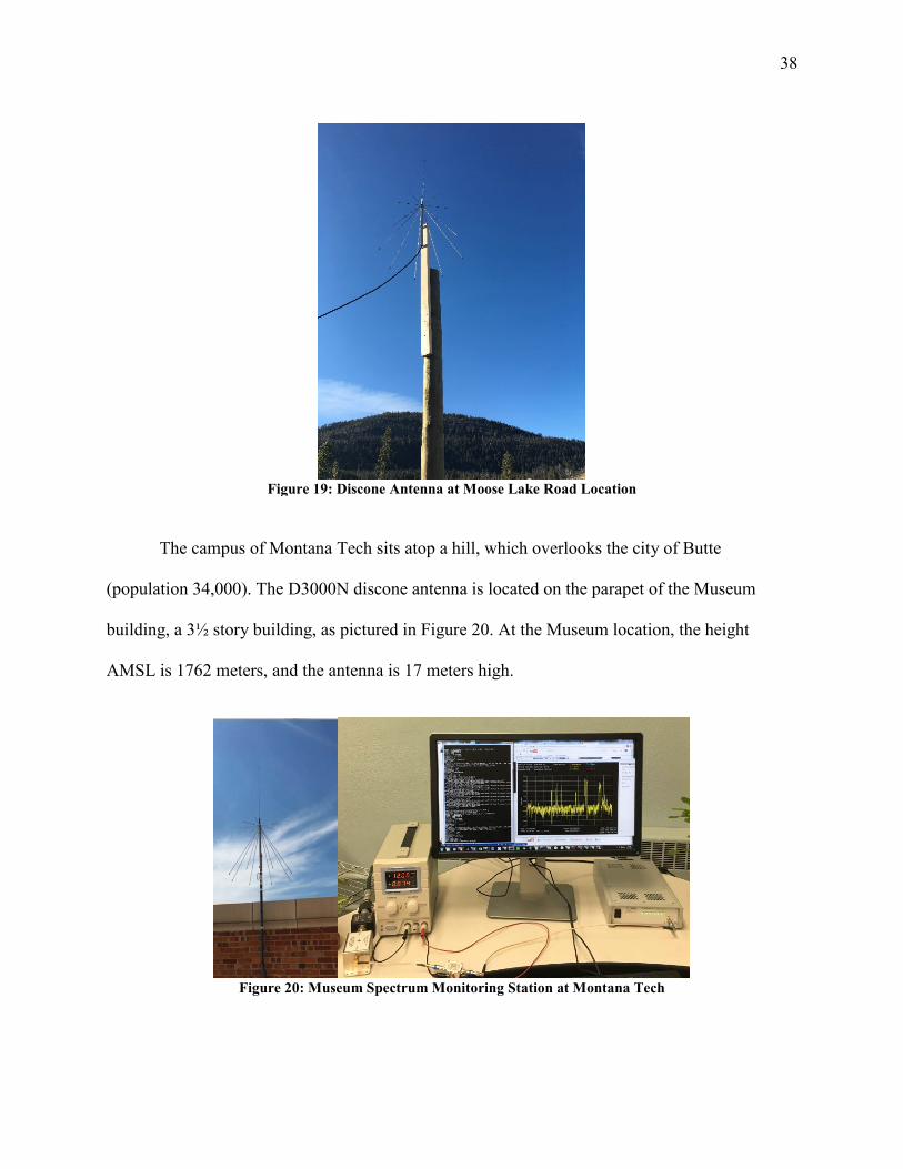
38

Figure 19: Discone Antenna at Moose Lake Road Location

The campus of Montana Tech sits atop a hill, which overlooks the city of Butte

(population 34,000). The D3000N discone antenna is located on the parapet of the Museum

building, a 3½ story building, as pictured in Figure 20. At the Museum location, the height

AMSL is 1762 meters, and the antenna is 17 meters high.

Figure 20: Museum Spectrum Monitoring Station at Montana Tech

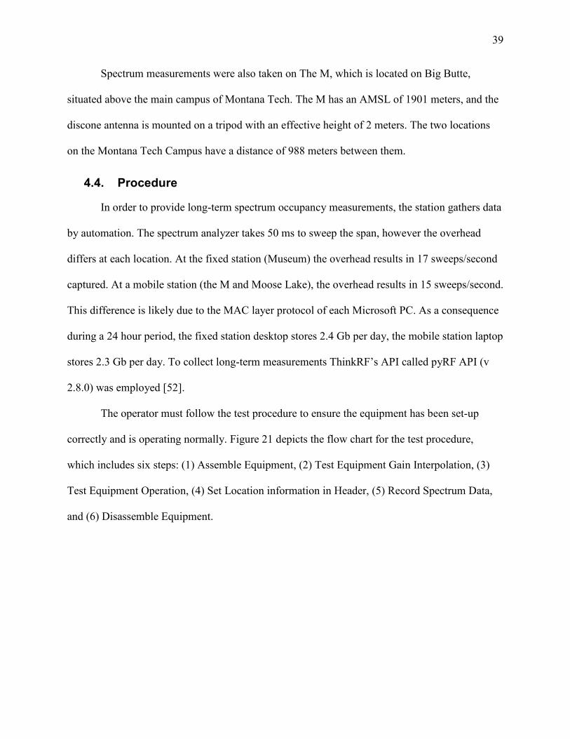
39

Spectrum measurements were also taken on The M, which is located on Big Butte,

situated above the main campus of Montana Tech. The M has an AMSL of 1901 meters, and the

discone antenna is mounted on a tripod with an effective height of 2 meters. The two locations

on the Montana Tech Campus have a distance of 988 meters between them.

4.4. Procedure

In order to provide long-term spectrum occupancy measurements, the station gathers data

by automation. The spectrum analyzer takes 50 ms to sweep the span, however the overhead

differs at each location. At the fixed station (Museum) the overhead results in 17 sweeps/second

captured. At a mobile station (the M and Moose Lake), the overhead results in 15 sweeps/second.

This difference is likely due to the MAC layer protocol of each Microsoft PC. As a consequence

during a 24 hour period, the fixed station desktop stores 2.4 Gb per day, the mobile station laptop

stores 2.3 Gb per day. To collect long-term measurements ThinkRF’s API called pyRF API (v

2.8.0) was employed [52].

The operator must follow the test procedure to ensure the equipment has been set-up

correctly and is operating normally. Figure 21 depicts the flow chart for the test procedure,

which includes six steps: (1) Assemble Equipment, (2) Test Equipment Gain Interpolation, (3)

Test Equipment Operation, (4) Set Location information in Header, (5) Record Spectrum Data,

and (6) Disassemble Equipment.

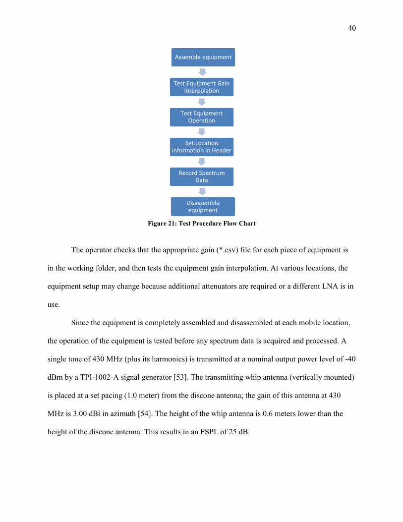
40

Figure 21: Test Procedure Flow Chart

The operator checks that the appropriate gain (*.csv) file for each piece of equipment is

in the working folder, and then tests the equipment gain interpolation. At various locations, the

equipment setup may change because additional attenuators are required or a different LNA is in

use.

Since the equipment is completely assembled and disassembled at each mobile location,

the operation of the equipment is tested before any spectrum data is acquired and processed. A

single tone of 430 MHz (plus its harmonics) is transmitted at a nominal output power level of -40

dBm by a TPI-1002-A signal generator [53]. The transmitting whip antenna (vertically mounted)

is placed at a set pacing (1.0 meter) from the discone antenna; the gain of this antenna at 430

MHz is 3.00 dBi in azimuth [54]. The height of the whip antenna is 0.6 meters lower than the

height of the discone antenna. This results in an FSPL of 25 dB.

Assemble equipment

Test Equipment Gain Interpolation

Test Equipment Operation

Set Location information in Header

Record Spectrum Data

Disassemble equipment

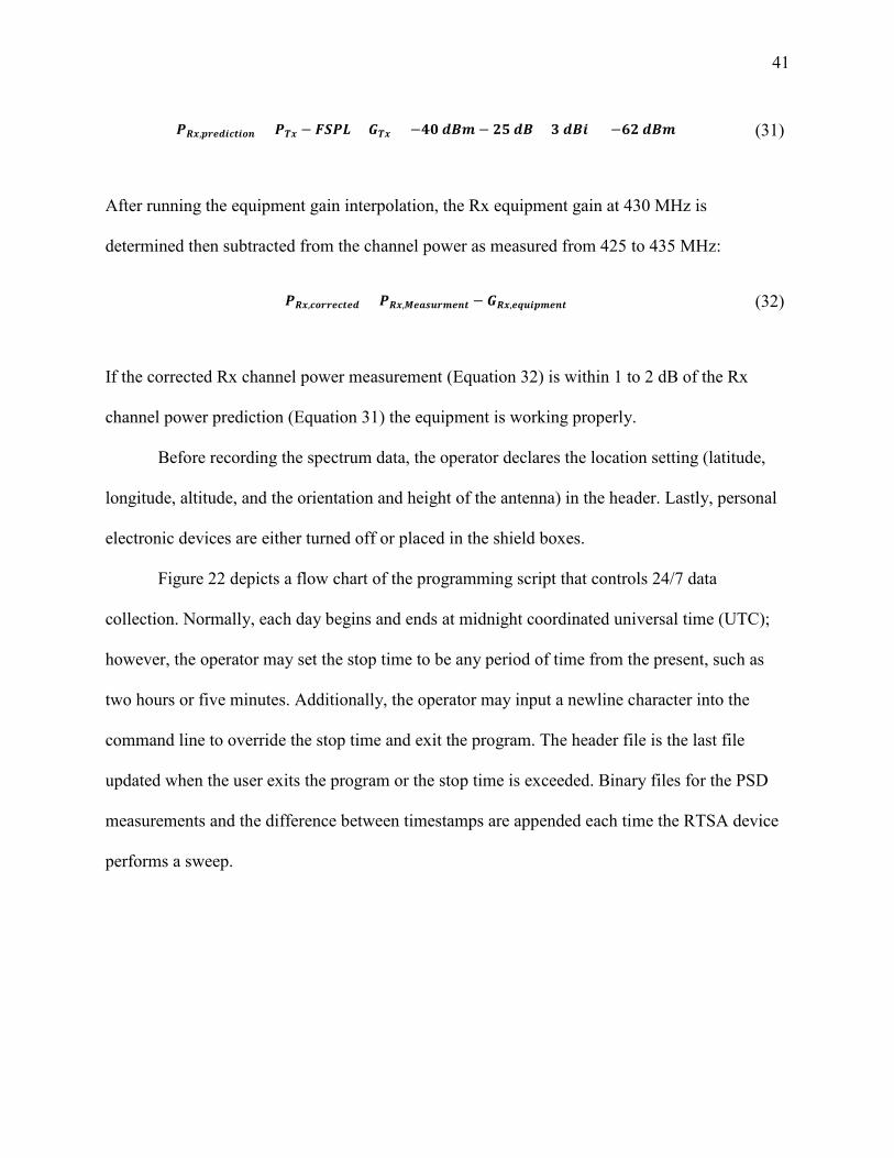
41

𝑷𝑷𝑬𝑬𝑻𝑻,𝒑𝒑𝒍𝒍𝒃𝒃𝒃𝒃𝒃𝒃𝒄𝒄𝒕𝒕𝒃𝒃𝒎𝒎𝒃𝒃 = 𝑷𝑷𝑻𝑻𝑻𝑻 − 𝑵𝑵𝑺𝑺𝑷𝑷𝑳𝑳 + 𝑮𝑮𝑻𝑻𝑻𝑻 = −𝟒𝟒𝟏𝟏 𝒃𝒃𝒅𝒅𝒎𝒎− 𝟐𝟐𝟐𝟐 𝒃𝒃𝒅𝒅 + 𝟑𝟑 𝒃𝒃𝒅𝒅𝒃𝒃 = −𝟔𝟔𝟐𝟐 𝒃𝒃𝒅𝒅𝒎𝒎 (31)

After running the equipment gain interpolation, the Rx equipment gain at 430 MHz is

determined then subtracted from the channel power as measured from 425 to 435 MHz:

𝑷𝑷𝑬𝑬𝑻𝑻,𝒄𝒄𝒎𝒎𝒍𝒍𝒍𝒍𝒃𝒃𝒄𝒄𝒕𝒕𝒃𝒃𝒃𝒃 = 𝑷𝑷𝑬𝑬𝑻𝑻,𝑴𝑴𝒃𝒃𝒃𝒃𝑵𝑵𝒎𝒎𝒍𝒍𝒎𝒎𝒃𝒃𝒃𝒃𝒕𝒕 − 𝑮𝑮𝑬𝑬𝑻𝑻,𝒃𝒃𝒆𝒆𝒎𝒎𝒃𝒃𝒑𝒑𝒎𝒎𝒃𝒃𝒃𝒃𝒕𝒕 (32)

If the corrected Rx channel power measurement (Equation 32) is within 1 to 2 dB of the Rx

channel power prediction (Equation 31) the equipment is working properly.

Before recording the spectrum data, the operator declares the location setting (latitude,

longitude, altitude, and the orientation and height of the antenna) in the header. Lastly, personal

electronic devices are either turned off or placed in the shield boxes.

Figure 22 depicts a flow chart of the programming script that controls 24/7 data

collection. Normally, each day begins and ends at midnight coordinated universal time (UTC);

however, the operator may set the stop time to be any period of time from the present, such as

two hours or five minutes. Additionally, the operator may input a newline character into the

command line to override the stop time and exit the program. The header file is the last file

updated when the user exits the program or the stop time is exceeded. Binary files for the PSD

measurements and the difference between timestamps are appended each time the RTSA device

performs a sweep.

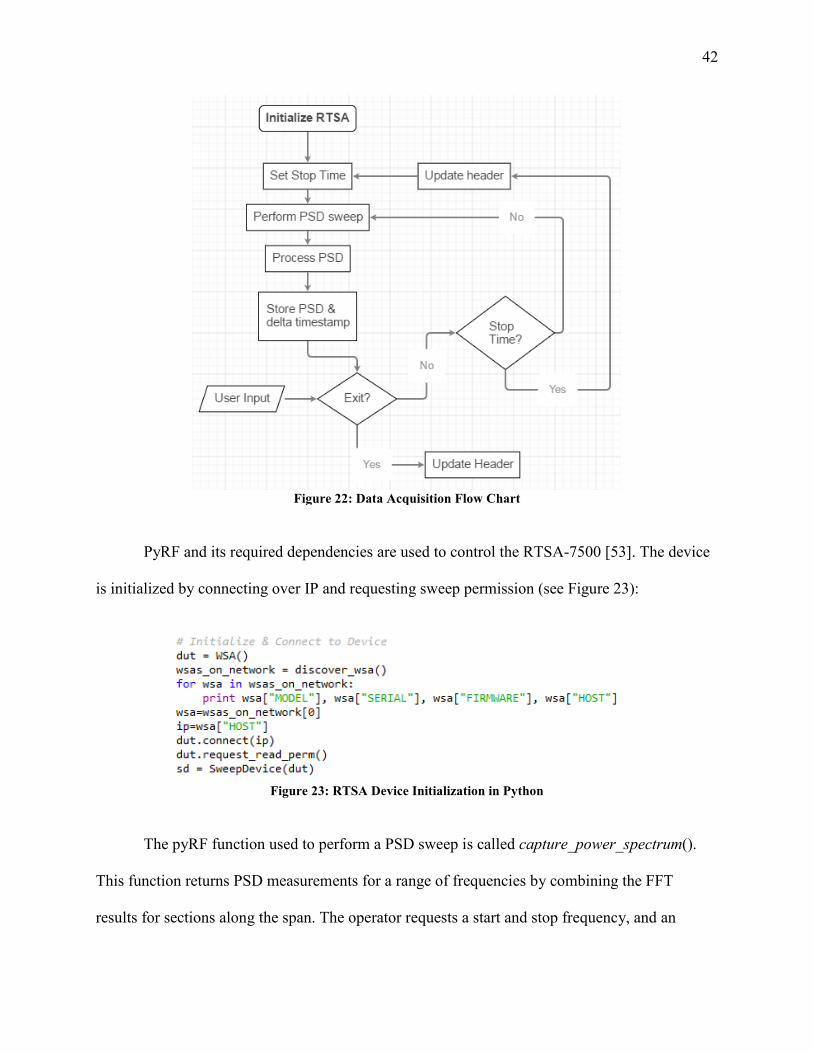
42

Figure 22: Data Acquisition Flow Chart

PyRF and its required dependencies are used to control the RTSA-7500 [53]. The device

is initialized by connecting over IP and requesting sweep permission (see Figure 23):

Figure 23: RTSA Device Initialization in Python

The pyRF function used to perform a PSD sweep is called capture_power_spectrum().

This function returns PSD measurements for a range of frequencies by combining the FFT

results for sections along the span. The operator requests a start and stop frequency, and an

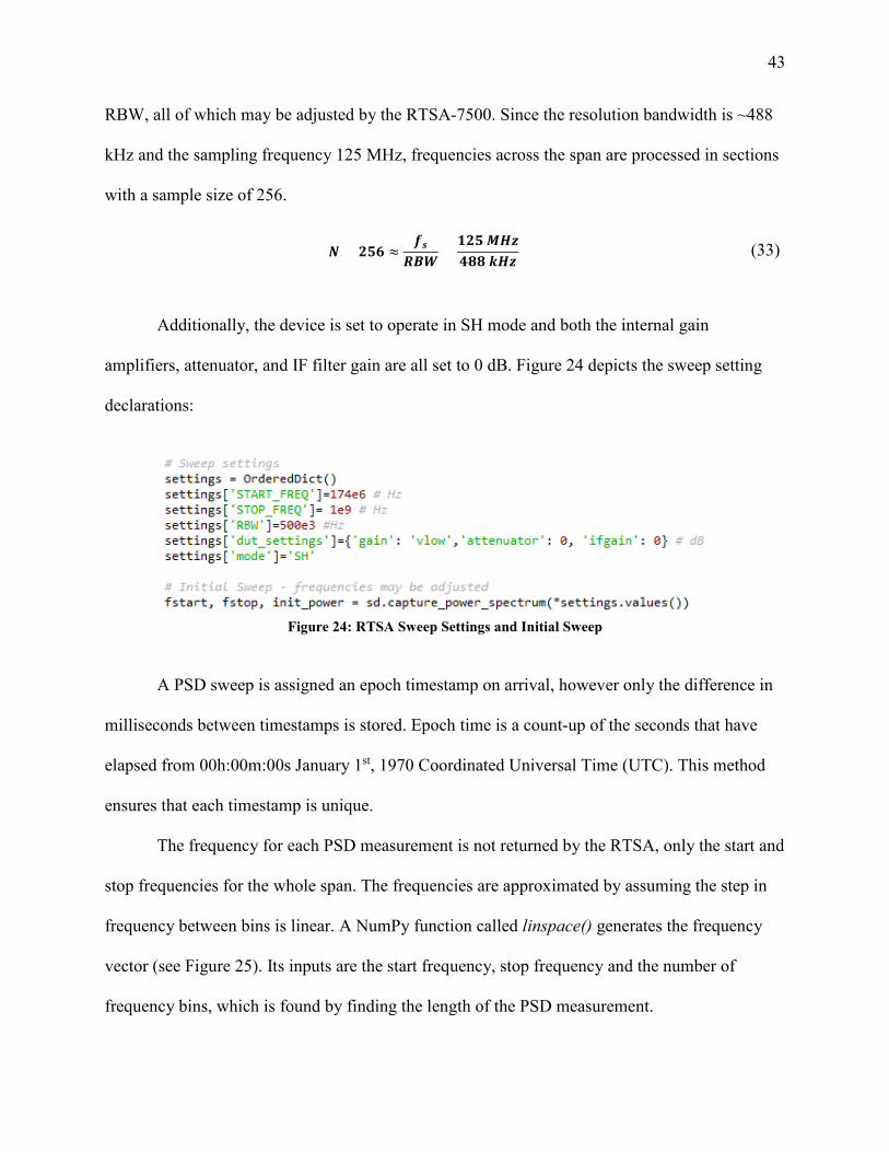
43

RBW, all of which may be adjusted by the RTSA-7500. Since the resolution bandwidth is ~488

kHz and the sampling frequency 125 MHz, frequencies across the span are processed in sections

with a sample size of 256.

𝑵𝑵 = 𝟐𝟐𝟐𝟐𝟔𝟔 ≈𝟐𝟐𝑵𝑵

𝑬𝑬𝒅𝒅𝒅𝒅=𝟏𝟏𝟐𝟐𝟐𝟐 𝑴𝑴𝑯𝑯𝑯𝑯𝟒𝟒𝟖𝟖𝟖𝟖 𝒌𝒌𝑯𝑯𝑯𝑯

(33)

Additionally, the device is set to operate in SH mode and both the internal gain

amplifiers, attenuator, and IF filter gain are all set to 0 dB. Figure 24 depicts the sweep setting

declarations:

Figure 24: RTSA Sweep Settings and Initial Sweep

A PSD sweep is assigned an epoch timestamp on arrival, however only the difference in

milliseconds between timestamps is stored. Epoch time is a count-up of the seconds that have

elapsed from 00h:00m:00s January 1st, 1970 Coordinated Universal Time (UTC). This method

ensures that each timestamp is unique.

The frequency for each PSD measurement is not returned by the RTSA, only the start and

stop frequencies for the whole span. The frequencies are approximated by assuming the step in

frequency between bins is linear. A NumPy function called linspace() generates the frequency

vector (see Figure 25). Its inputs are the start frequency, stop frequency and the number of

frequency bins, which is found by finding the length of the PSD measurement.

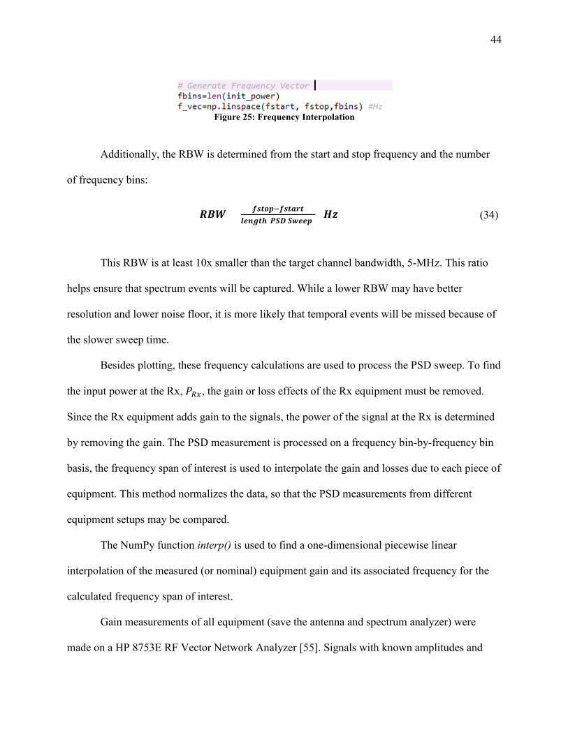
44

Figure 25: Frequency Interpolation

Additionally, the RBW is determined from the start and stop frequency and the number

of frequency bins:

𝑬𝑬𝒅𝒅𝒅𝒅 = 𝟐𝟐𝑵𝑵𝒕𝒕𝒎𝒎𝒑𝒑−𝟐𝟐𝑵𝑵𝒕𝒕𝒃𝒃𝒍𝒍𝒕𝒕𝒎𝒎𝒃𝒃𝒃𝒃𝒈𝒈𝒕𝒕𝒃𝒃(𝑷𝑷𝑺𝑺𝑫𝑫 𝑺𝑺𝒃𝒃𝒃𝒃𝒃𝒃𝒑𝒑) [𝑯𝑯𝑯𝑯] (34)

This RBW is at least 10x smaller than the target channel bandwidth, 5-MHz. This ratio

helps ensure that spectrum events will be captured. While a lower RBW may have better

resolution and lower noise floor, it is more likely that temporal events will be missed because of

the slower sweep time.

Besides plotting, these frequency calculations are used to process the PSD sweep. To find

the input power at the Rx, 𝑃𝑃𝑅𝑅𝑇𝑇, the gain or loss effects of the Rx equipment must be removed.

Since the Rx equipment adds gain to the signals, the power of the signal at the Rx is determined

by removing the gain. The PSD measurement is processed on a frequency bin-by-frequency bin

basis, the frequency span of interest is used to interpolate the gain and losses due to each piece of

equipment. This method normalizes the data, so that the PSD measurements from different

equipment setups may be compared.

The NumPy function interp() is used to find a one-dimensional piecewise linear

interpolation of the measured (or nominal) equipment gain and its associated frequency for the

calculated frequency span of interest.

Gain measurements of all equipment (save the antenna and spectrum analyzer) were

made on a HP 8753E RF Vector Network Analyzer [55]. Signals with known amplitudes and

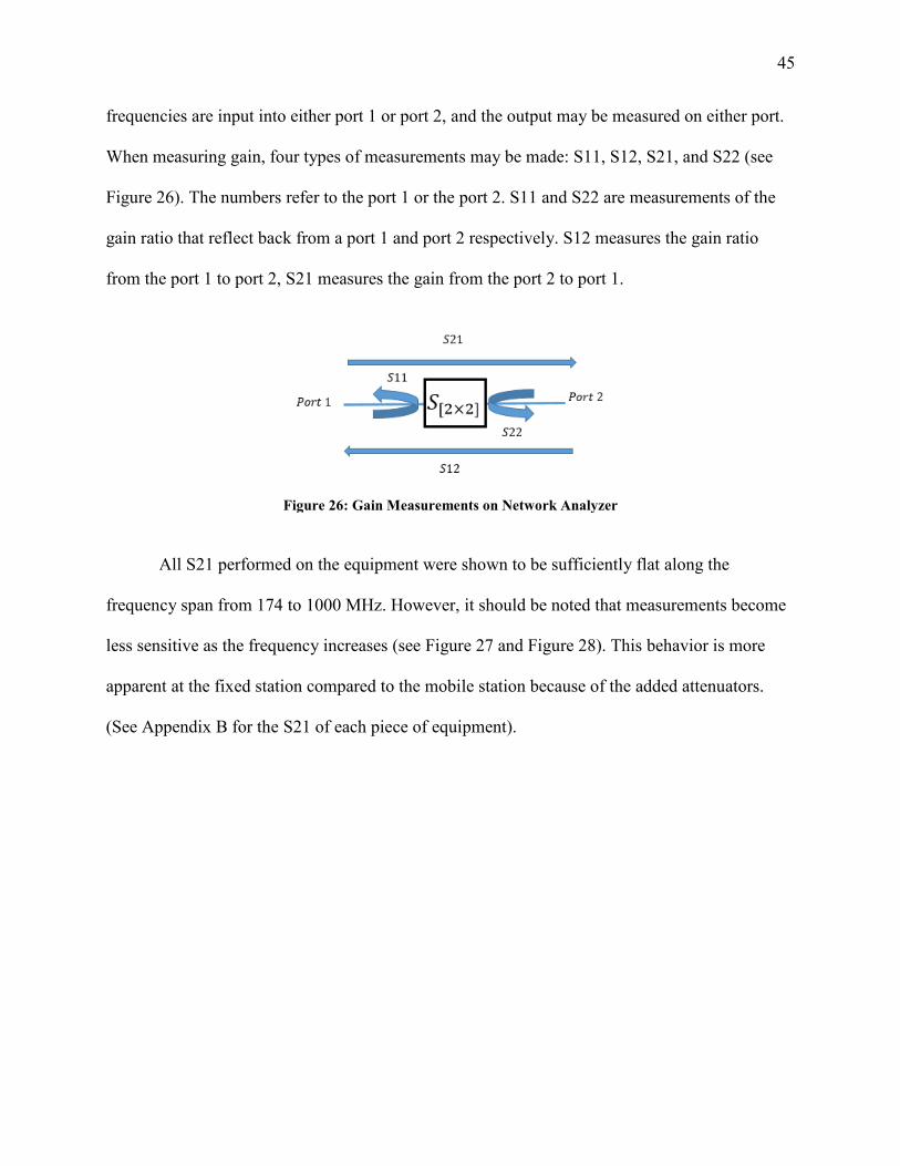
45

frequencies are input into either port 1 or port 2, and the output may be measured on either port.

When measuring gain, four types of measurements may be made: S11, S12, S21, and S22 (see

Figure 26). The numbers refer to the port 1 or the port 2. S11 and S22 are measurements of the

gain ratio that reflect back from a port 1 and port 2 respectively. S12 measures the gain ratio

from the port 1 to port 2, S21 measures the gain from the port 2 to port 1.

Figure 26: Gain Measurements on Network Analyzer

All S21 performed on the equipment were shown to be sufficiently flat along the

frequency span from 174 to 1000 MHz. However, it should be noted that measurements become

less sensitive as the frequency increases (see Figure 27 and Figure 28). This behavior is more

apparent at the fixed station compared to the mobile station because of the added attenuators.

(See Appendix B for the S21 of each piece of equipment).

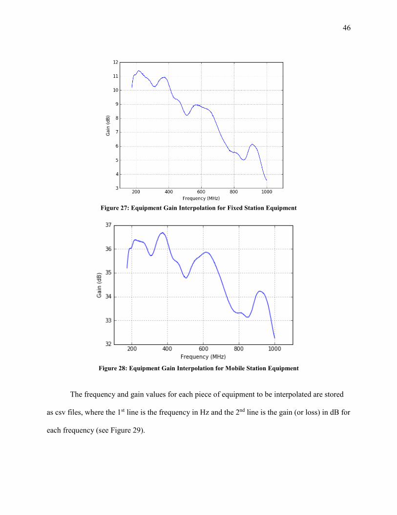
46

Figure 27: Equipment Gain Interpolation for Fixed Station Equipment

Figure 28: Equipment Gain Interpolation for Mobile Station Equipment

The frequency and gain values for each piece of equipment to be interpolated are stored

as csv files, where the 1st line is the frequency in Hz and the 2nd line is the gain (or loss) in dB for

each frequency (see Figure 29).

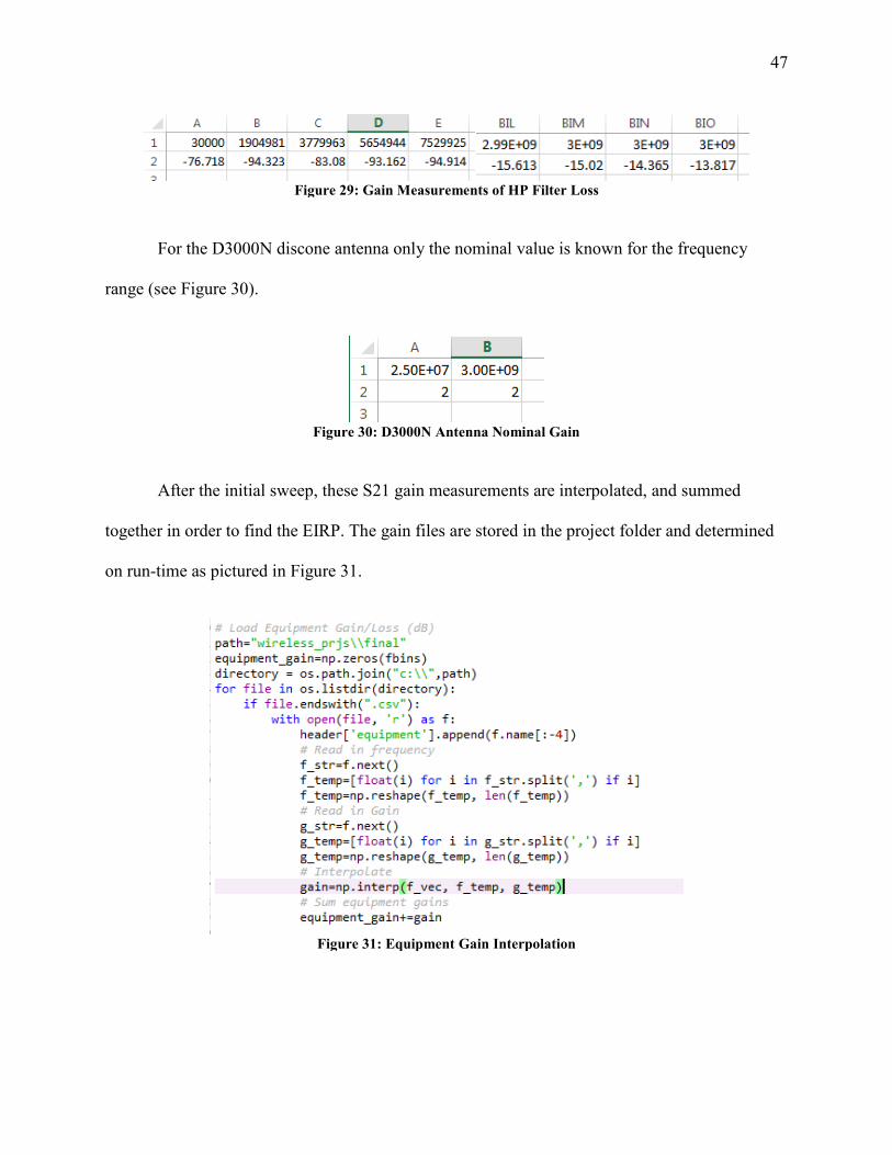
47

Figure 29: Gain Measurements of HP Filter Loss

For the D3000N discone antenna only the nominal value is known for the frequency

range (see Figure 30).

Figure 30: D3000N Antenna Nominal Gain

After the initial sweep, these S21 gain measurements are interpolated, and summed

together in order to find the EIRP. The gain files are stored in the project folder and determined

on run-time as pictured in Figure 31.

Figure 31: Equipment Gain Interpolation

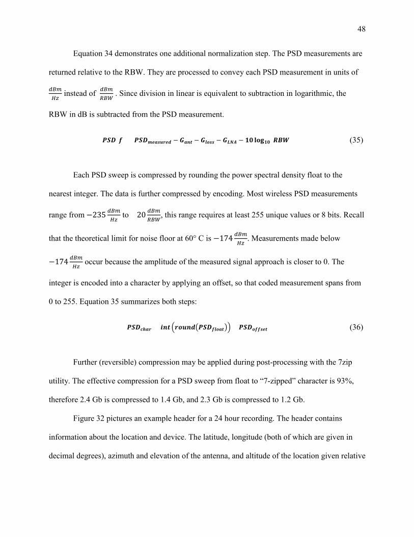
48

Equation 34 demonstrates one additional normalization step. The PSD measurements are

returned relative to the RBW. They are processed to convey each PSD measurement in units of

𝑏𝑏𝑑𝑑𝑚𝑚𝐻𝐻𝐻𝐻

instead of 𝑏𝑏𝑑𝑑𝑚𝑚𝑅𝑅𝑑𝑑𝑚𝑚

. Since division in linear is equivalent to subtraction in logarithmic, the

RBW in dB is subtracted from the PSD measurement.

𝑷𝑷𝑺𝑺𝑫𝑫(𝟐𝟐) = 𝑷𝑷𝑺𝑺𝑫𝑫𝒎𝒎𝒃𝒃𝒃𝒃𝑵𝑵𝒎𝒎𝒍𝒍𝒃𝒃𝒃𝒃 − 𝑮𝑮𝒃𝒃𝒃𝒃𝒕𝒕 − 𝑮𝑮𝒎𝒎𝒎𝒎𝑵𝑵𝑵𝑵 − 𝑮𝑮𝑳𝑳𝑵𝑵𝑨𝑨 − 𝟏𝟏𝟏𝟏 𝐥𝐥𝐜𝐜𝐥𝐥𝟏𝟏𝟏𝟏(𝑬𝑬𝒅𝒅𝒅𝒅) (35)

Each PSD sweep is compressed by rounding the power spectral density float to the

nearest integer. The data is further compressed by encoding. Most wireless PSD measurements

range from −235 𝑏𝑏𝑑𝑑𝑚𝑚𝐻𝐻𝐻𝐻

to +20 𝑏𝑏𝑑𝑑𝑚𝑚𝑅𝑅𝑑𝑑𝑚𝑚

, this range requires at least 255 unique values or 8 bits. Recall

that the theoretical limit for noise floor at 60° C is −174 𝑏𝑏𝑑𝑑𝑚𝑚𝐻𝐻𝐻𝐻

. Measurements made below

−174 𝑏𝑏𝑑𝑑𝑚𝑚𝐻𝐻𝐻𝐻

occur because the amplitude of the measured signal approach is closer to 0. The

integer is encoded into a character by applying an offset, so that coded measurement spans from

0 to 255. Equation 35 summarizes both steps:

𝑷𝑷𝑺𝑺𝑫𝑫𝒄𝒄𝒃𝒃𝒃𝒃𝒍𝒍 = 𝒃𝒃𝒃𝒃𝒕𝒕 �𝒍𝒍𝒎𝒎𝒎𝒎𝒃𝒃𝒃𝒃�𝑷𝑷𝑺𝑺𝑫𝑫𝟐𝟐𝒎𝒎𝒎𝒎𝒃𝒃𝒕𝒕�� + 𝑷𝑷𝑺𝑺𝑫𝑫𝒎𝒎𝟐𝟐𝟐𝟐𝑵𝑵𝒃𝒃𝒕𝒕 (36)

Further (reversible) compression may be applied during post-processing with the 7zip

utility. The effective compression for a PSD sweep from float to “7-zipped” character is 93%,

therefore 2.4 Gb is compressed to 1.4 Gb, and 2.3 Gb is compressed to 1.2 Gb.

Figure 32 pictures an example header for a 24 hour recording. The header contains

information about the location and device. The latitude, longitude (both of which are given in

decimal degrees), azimuth and elevation of the antenna, and altitude of the location given relative

49

to sea-level (ASML) and ground (AGL) are set by the operator. The initial and last timestamps

are given in epoch time in milliseconds, but the filename is epoch time in seconds.

Figure 32: Typical Header File

For the desktop at the fixed station, the number of sweeps of 1.48 million is typical for a

24 hour recording. For the laptop used in the mobile station, the number of sweeps is 1.29

million. This count is necessary to access and the binary files for the PSD measurements and

delta timestamps. Since the data is homogenous, the data can be quickly read and written using

the Python module array [56] (see Figure 33). However, both the binary format and the number

of binary must be known to access and index the array. This method does not load the data into

memory, but creates a map for quick access.

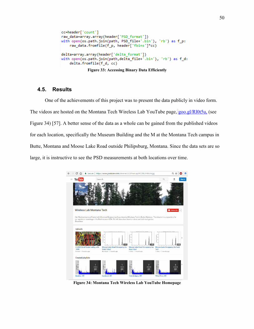
50

Figure 33: Accessing Binary Data Efficiently

4.5. Results

One of the achievements of this project was to present the data publicly in video form.

The videos are hosted on the Montana Tech Wireless Lab YouTube page, goo.gl/Rl0t5u, (see

Figure 34) [57]. A better sense of the data as a whole can be gained from the published videos

for each location, specifically the Museum Building and the M at the Montana Tech campus in

Butte, Montana and Moose Lake Road outside Philipsburg, Montana. Since the data sets are so

large, it is instructive to see the PSD measurements at both locations over time.

Figure 34: Montana Tech Wireless Lab YouTube Homepage

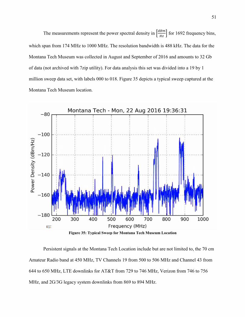
51

The measurements represent the power spectral density in �𝑏𝑏𝑑𝑑𝑚𝑚𝐻𝐻𝐻𝐻

� for 1692 frequency bins,

which span from 174 MHz to 1000 MHz. The resolution bandwidth is 488 kHz. The data for the

Montana Tech Museum was collected in August and September of 2016 and amounts to 32 Gb

of data (not archived with 7zip utility). For data analysis this set was divided into a 19 by 1

million sweep data set, with labels 000 to 018. Figure 35 depicts a typical sweep captured at the

Montana Tech Museum location.

Figure 35: Typical Sweep for Montana Tech Museum Location

Persistent signals at the Montana Tech Location include but are not limited to, the 70 cm

Amateur Radio band at 450 MHz, TV Channels 19 from 500 to 506 MHz and Channel 43 from

644 to 650 MHz, LTE downlinks for AT&T from 729 to 746 MHz, Verizon from 746 to 756

MHz, and 2G/3G legacy system downlinks from 869 to 894 MHz.

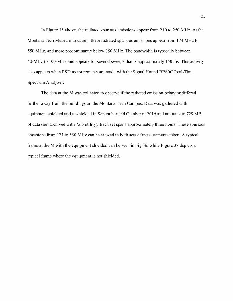
52

In Figure 35 above, the radiated spurious emissions appear from 210 to 250 MHz. At the

Montana Tech Museum Location, these radiated spurious emissions appear from 174 MHz to

550 MHz, and more predominantly below 350 MHz. The bandwidth is typically between

40-MHz to 100-MHz and appears for several sweeps that is approximately 150 ms. This activity

also appears when PSD measurements are made with the Signal Hound BB60C Real-Time

Spectrum Analyzer.

The data at the M was collected to observe if the radiated emission behavior differed

further away from the buildings on the Montana Tech Campus. Data was gathered with

equipment shielded and unshielded in September and October of 2016 and amounts to 729 MB

of data (not archived with 7zip utility). Each set spans approximately three hours. These spurious

emissions from 174 to 550 MHz can be viewed in both sets of measurements taken. A typical

frame at the M with the equipment shielded can be seen in Fig 36, while Figure 37 depicts a

typical frame where the equipment is not shielded.

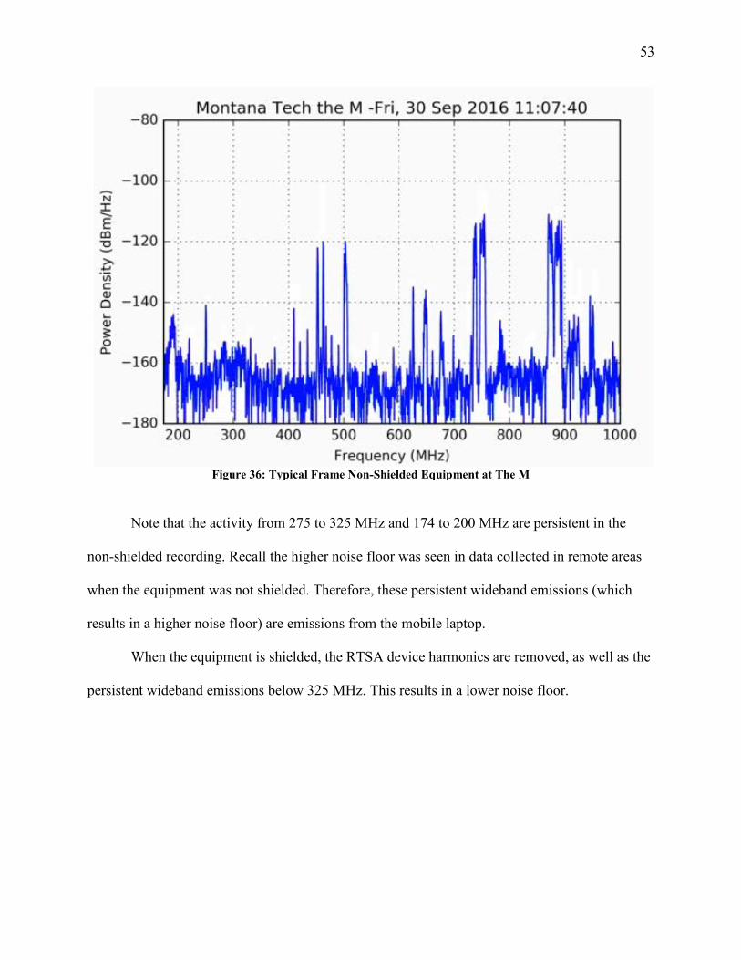
53

Figure 36: Typical Frame Non-Shielded Equipment at The M

Note that the activity from 275 to 325 MHz and 174 to 200 MHz are persistent in the

non-shielded recording. Recall the higher noise floor was seen in data collected in remote areas

when the equipment was not shielded. Therefore, these persistent wideband emissions (which

results in a higher noise floor) are emissions from the mobile laptop.

When the equipment is shielded, the RTSA device harmonics are removed, as well as the

persistent wideband emissions below 325 MHz. This results in a lower noise floor.

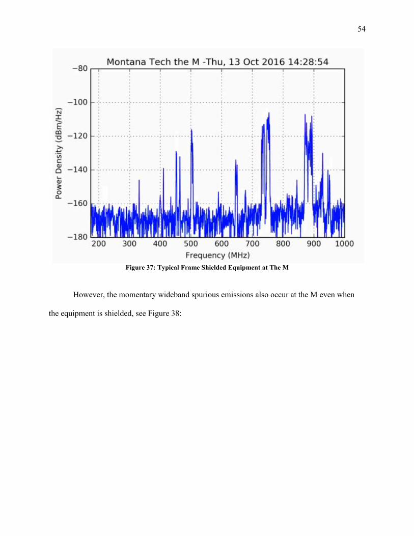
54

Figure 37: Typical Frame Shielded Equipment at The M

However, the momentary wideband spurious emissions also occur at the M even when

the equipment is shielded, see Figure 38:

55

Figure 38: The M Sweep with Spurious Emissions

Initially, it was assumed that bands below 500 MHz were viable for testing a mobile

broadband network. These pathological spurious emissions make these bands less valuable.

At the remote location, Moose Lake, the data was collected in November of 2016 for 2

weeks, which amounts to 29 Gb of data (not archived with 7zip utility). For data analysis, this set

was divided into 17 by 1 million sweep data set, with labels 000 to 016. Figure 39 depicts a

typical sweep captured by the RTSA:

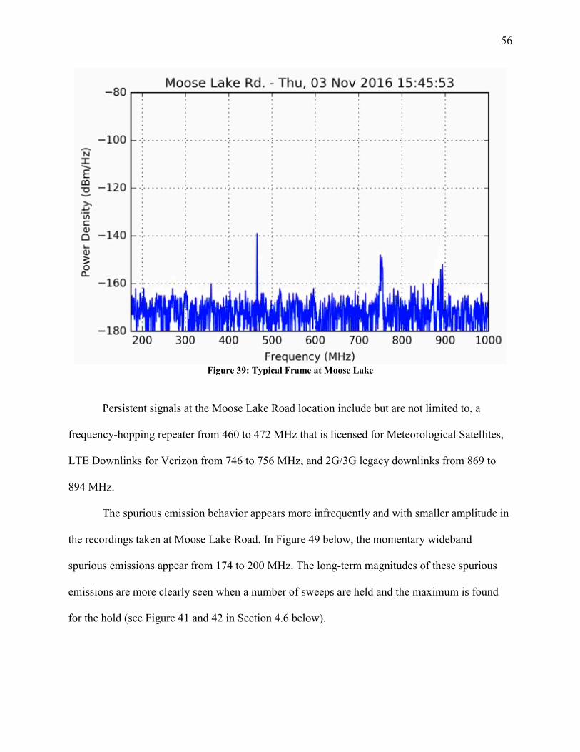
56

Figure 39: Typical Frame at Moose Lake

Persistent signals at the Moose Lake Road location include but are not limited to, a

frequency-hopping repeater from 460 to 472 MHz that is licensed for Meteorological Satellites,

LTE Downlinks for Verizon from 746 to 756 MHz, and 2G/3G legacy downlinks from 869 to

894 MHz.

The spurious emission behavior appears more infrequently and with smaller amplitude in

the recordings taken at Moose Lake Road. In Figure 49 below, the momentary wideband

spurious emissions appear from 174 to 200 MHz. The long-term magnitudes of these spurious

emissions are more clearly seen when a number of sweeps are held and the maximum is found

for the hold (see Figure 41 and 42 in Section 4.6 below).

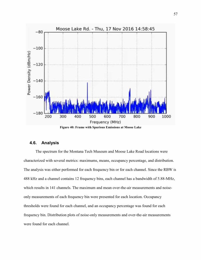
57

Figure 40: Frame with Spurious Emissions at Moose Lake

4.6. Analysis

The spectrum for the Montana Tech Museum and Moose Lake Road locations were

characterized with several metrics: maximums, means, occupancy percentage, and distribution.

The analysis was either performed for each frequency bin or for each channel. Since the RBW is

488 kHz and a channel contains 12 frequency bins, each channel has a bandwidth of 5.88-MHz,

which results in 141 channels. The maximum and mean over-the-air measurements and noise-

only measurements of each frequency bin were presented for each location. Occupancy

thresholds were found for each channel, and an occupancy percentage was found for each

frequency bin. Distribution plots of noise-only measurements and over-the-air measurements

were found for each channel.

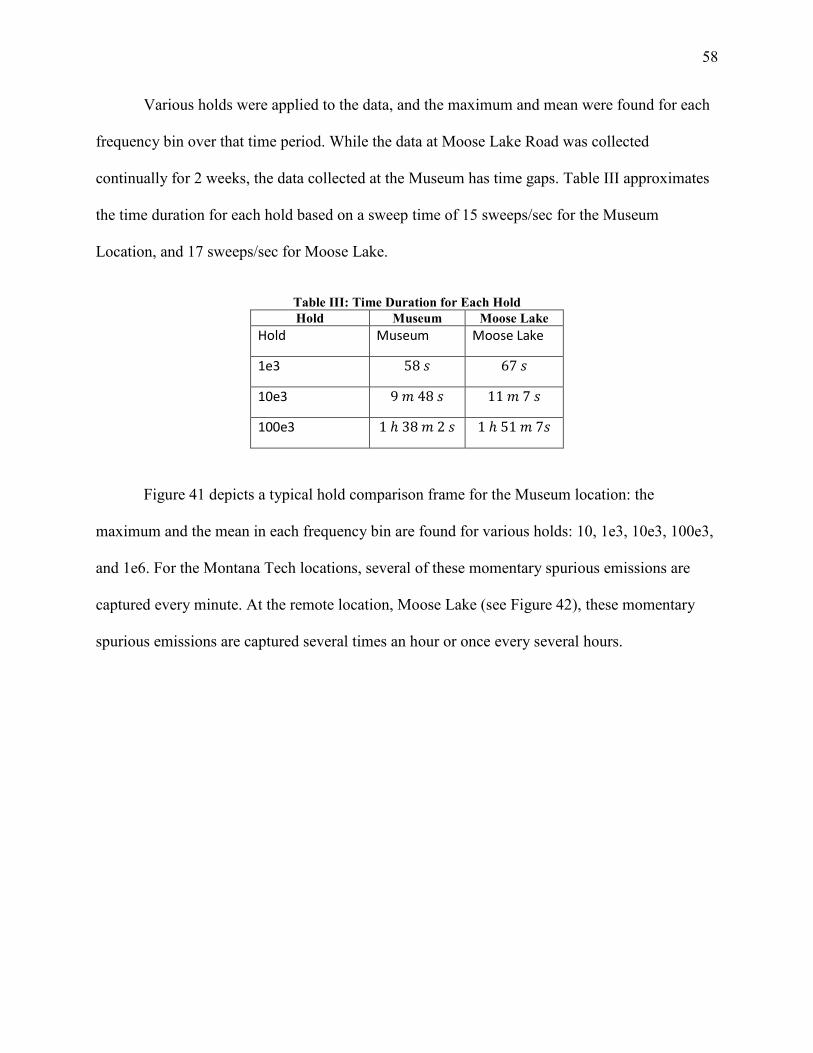
58

Various holds were applied to the data, and the maximum and mean were found for each

frequency bin over that time period. While the data at Moose Lake Road was collected

continually for 2 weeks, the data collected at the Museum has time gaps. Table III approximates

the time duration for each hold based on a sweep time of 15 sweeps/sec for the Museum

Location, and 17 sweeps/sec for Moose Lake.

Table III: Time Duration for Each Hold Hold Museum Moose Lake

Hold Museum Moose Lake

1e3 58 𝐿𝐿 67 𝐿𝐿

10e3 9 𝑑𝑑 48 𝐿𝐿 11 𝑑𝑑 7 𝐿𝐿

100e3 1 ℎ 38 𝑑𝑑 2 𝐿𝐿 1 ℎ 51 𝑑𝑑 7𝐿𝐿

Figure 41 depicts a typical hold comparison frame for the Museum location: the

maximum and the mean in each frequency bin are found for various holds: 10, 1e3, 10e3, 100e3,

and 1e6. For the Montana Tech locations, several of these momentary spurious emissions are

captured every minute. At the remote location, Moose Lake (see Figure 42), these momentary

spurious emissions are captured several times an hour or once every several hours.

59

Figure 41: Montana Tech Museum Hold Comparison

Besides the persistent signals described earlier, other notable activity at the Montana

Tech location occurred in the industrial, scientific and medical (ISM) radio band from 902 to 928

MHz. This band is used by low-powered unlicensed devices. This band is called the 33-cm band

by Amateur Radio operators, who are licensed to use this band on a secondary basis. In this

band, the devices appear to perform frequency-hopping to find an available channel. There is

also activity from 942 to 955 MHz, which is allocated for fixed communications. In Butte,

Montana this may be used by aural broadcast auxiliary stations in order to transmit from the

studio to the broadcast transmitter.

Besides the 70 cm Amateur Radio in use from 450 to 455 MHz, the Amateur Radio

1.25 m band is also in use from 223 to 235 MHz. The signal at 220 MHz is located in a TV

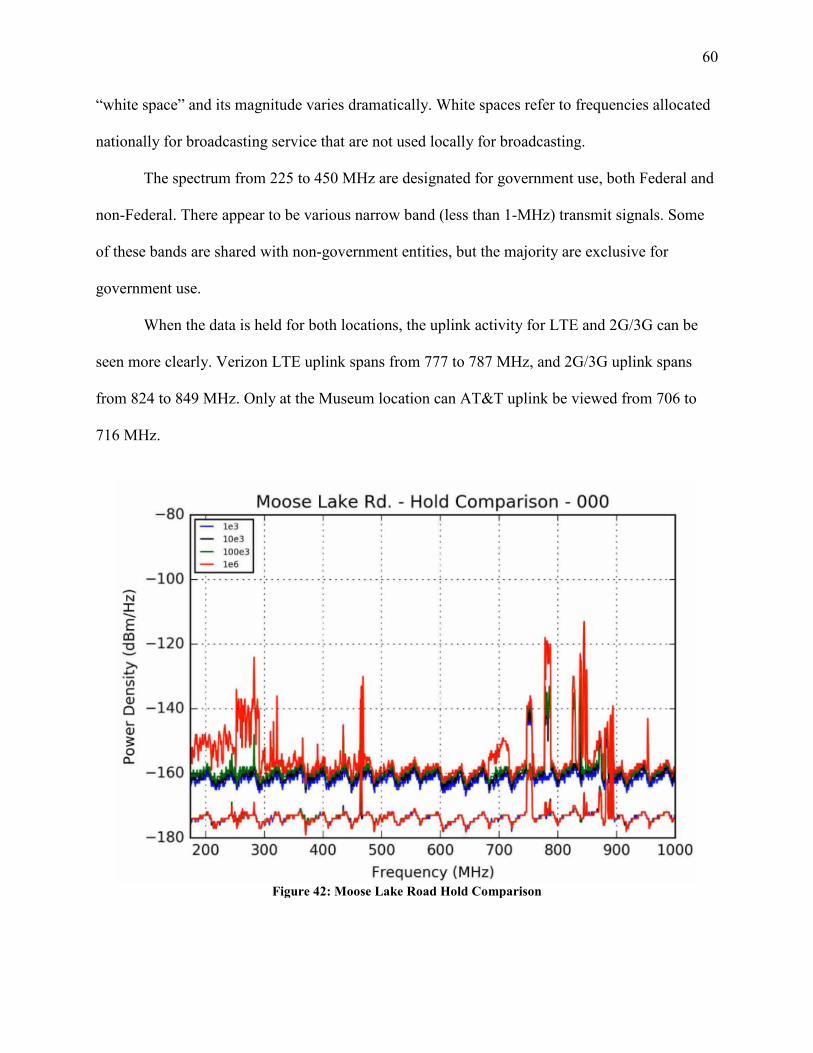
60

“white space” and its magnitude varies dramatically. White spaces refer to frequencies allocated

nationally for broadcasting service that are not used locally for broadcasting.

The spectrum from 225 to 450 MHz are designated for government use, both Federal and

non-Federal. There appear to be various narrow band (less than 1-MHz) transmit signals. Some

of these bands are shared with non-government entities, but the majority are exclusive for

government use.

When the data is held for both locations, the uplink activity for LTE and 2G/3G can be

seen more clearly. Verizon LTE uplink spans from 777 to 787 MHz, and 2G/3G uplink spans

from 824 to 849 MHz. Only at the Museum location can AT&T uplink be viewed from 706 to

716 MHz.

Figure 42: Moose Lake Road Hold Comparison

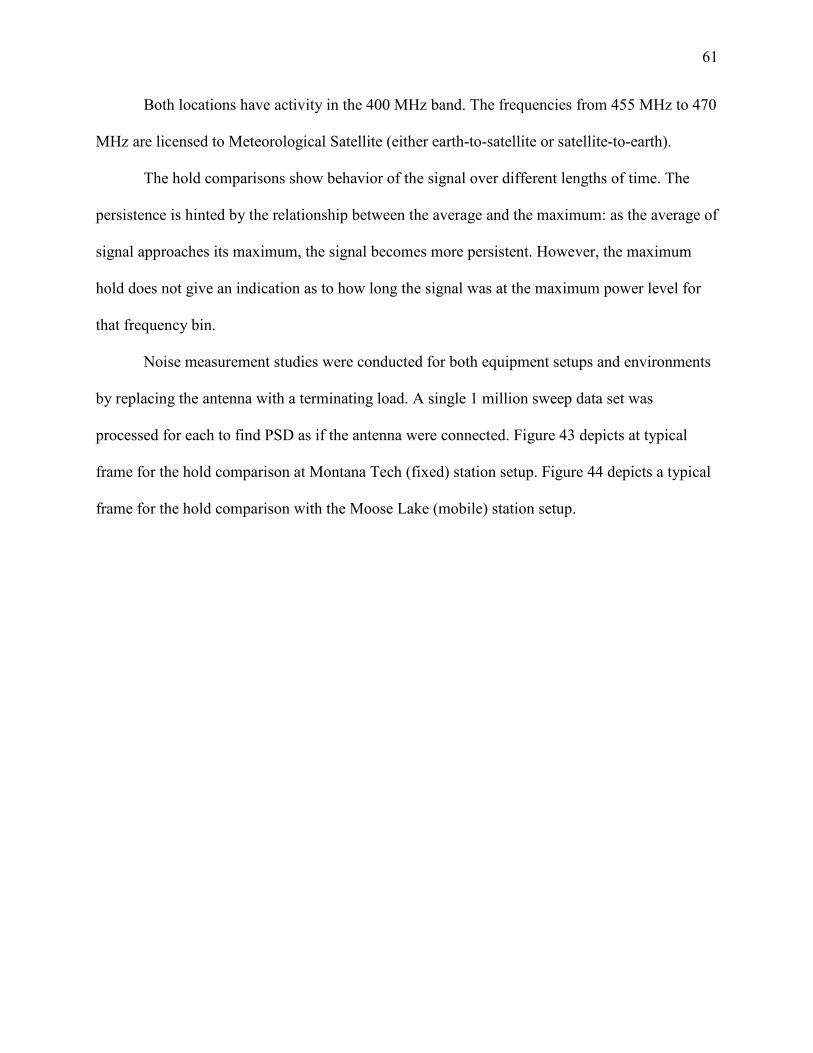
61

Both locations have activity in the 400 MHz band. The frequencies from 455 MHz to 470

MHz are licensed to Meteorological Satellite (either earth-to-satellite or satellite-to-earth).

The hold comparisons show behavior of the signal over different lengths of time. The

persistence is hinted by the relationship between the average and the maximum: as the average of

signal approaches its maximum, the signal becomes more persistent. However, the maximum

hold does not give an indication as to how long the signal was at the maximum power level for

that frequency bin.

Noise measurement studies were conducted for both equipment setups and environments

by replacing the antenna with a terminating load. A single 1 million sweep data set was

processed for each to find PSD as if the antenna were connected. Figure 43 depicts at typical

frame for the hold comparison at Montana Tech (fixed) station setup. Figure 44 depicts a typical

frame for the hold comparison with the Moose Lake (mobile) station setup.

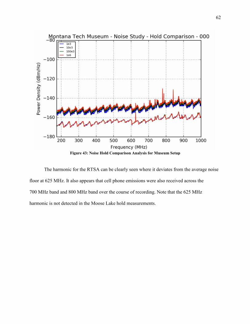
62

Figure 43: Noise Hold Comparison Analysis for Museum Setup

The harmonic for the RTSA can be clearly seen where it deviates from the average noise

floor at 625 MHz. It also appears that cell phone emissions were also received across the

700 MHz band and 800 MHz band over the course of recording. Note that the 625 MHz

harmonic is not detected in the Moose Lake hold measurements.

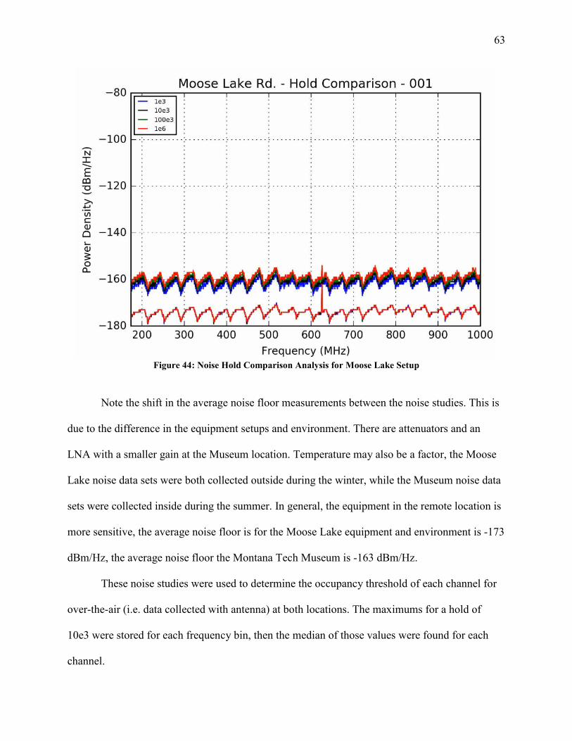
63

Figure 44: Noise Hold Comparison Analysis for Moose Lake Setup

Note the shift in the average noise floor measurements between the noise studies. This is

due to the difference in the equipment setups and environment. There are attenuators and an

LNA with a smaller gain at the Museum location. Temperature may also be a factor, the Moose

Lake noise data sets were both collected outside during the winter, while the Museum noise data

sets were collected inside during the summer. In general, the equipment in the remote location is

more sensitive, the average noise floor is for the Moose Lake equipment and environment is -173

dBm/Hz, the average noise floor the Montana Tech Museum is -163 dBm/Hz.

These noise studies were used to determine the occupancy threshold of each channel for

over-the-air (i.e. data collected with antenna) at both locations. The maximums for a hold of

10e3 were stored for each frequency bin, then the median of those values were found for each

channel.

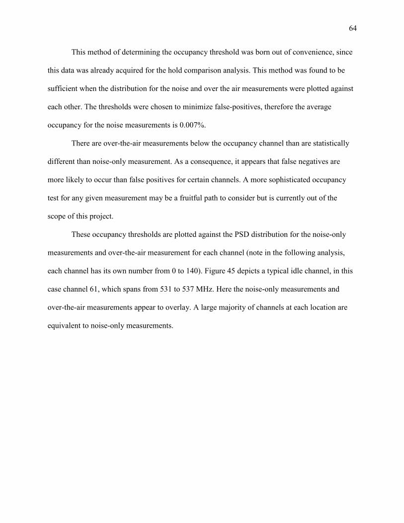
64

This method of determining the occupancy threshold was born out of convenience, since

this data was already acquired for the hold comparison analysis. This method was found to be

sufficient when the distribution for the noise and over the air measurements were plotted against

each other. The thresholds were chosen to minimize false-positives, therefore the average

occupancy for the noise measurements is 0.007%.

There are over-the-air measurements below the occupancy channel than are statistically

different than noise-only measurement. As a consequence, it appears that false negatives are

more likely to occur than false positives for certain channels. A more sophisticated occupancy

test for any given measurement may be a fruitful path to consider but is currently out of the

scope of this project.

These occupancy thresholds are plotted against the PSD distribution for the noise-only

measurements and over-the-air measurement for each channel (note in the following analysis,

each channel has its own number from 0 to 140). Figure 45 depicts a typical idle channel, in this

case channel 61, which spans from 531 to 537 MHz. Here the noise-only measurements and

over-the-air measurements appear to overlay. A large majority of channels at each location are

equivalent to noise-only measurements.

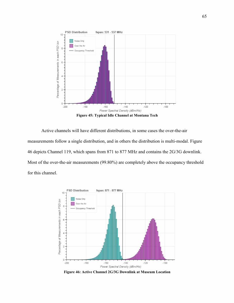
65

Figure 45: Typical Idle Channel at Montana Tech

Active channels will have different distributions, in some cases the over-the-air

measurements follow a single distribution, and in others the distribution is multi-modal. Figure

46 depicts Channel 119, which spans from 871 to 877 MHz and contains the 2G/3G downlink.

Most of the over-the-air measurements (99.80%) are completely above the occupancy threshold

for this channel.

Figure 46: Active Channel 2G/3G Downlink at Museum Location

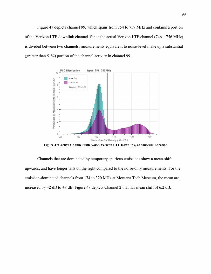
66

Figure 47 depicts channel 99, which spans from 754 to 759 MHz and contains a portion

of the Verizon LTE downlink channel. Since the actual Verizon LTE channel (746 – 756 MHz)

is divided between two channels, measurements equivalent to noise-level make up a substantial

(greater than 51%) portion of the channel activity in channel 99.

Figure 47: Active Channel with Noise, Verizon LTE Downlink, at Museum Location

Channels that are dominated by temporary spurious emissions show a mean-shift

upwards, and have longer tails on the right compared to the noise-only measurements. For the

emission-dominated channels from 174 to 320 MHz at Montana Tech Museum, the mean are

increased by +2 dB to +8 dB. Figure 48 depicts Channel 2 that has mean shift of 6.2 dB.

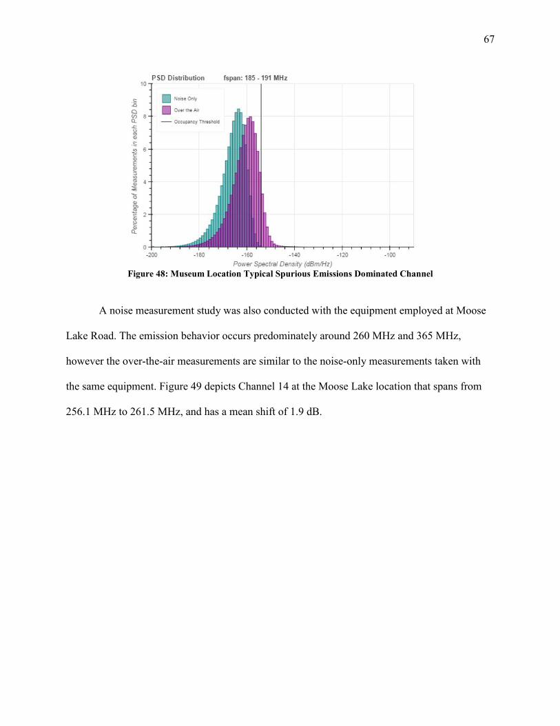
67

Figure 48: Museum Location Typical Spurious Emissions Dominated Channel

A noise measurement study was also conducted with the equipment employed at Moose

Lake Road. The emission behavior occurs predominately around 260 MHz and 365 MHz,

however the over-the-air measurements are similar to the noise-only measurements taken with

the same equipment. Figure 49 depicts Channel 14 at the Moose Lake location that spans from

256.1 MHz to 261.5 MHz, and has a mean shift of 1.9 dB.

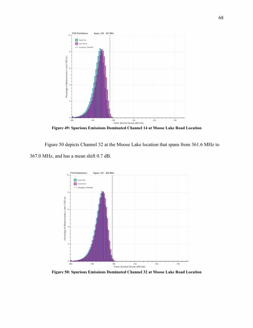
68

Figure 49: Spurious Emissions Dominated Channel 14 at Moose Lake Road Location

Figure 50 depicts Channel 32 at the Moose Lake location that spans from 361.6 MHz to

367.0 MHz, and has a mean shift 0.7 dB.

Figure 50: Spurious Emissions Dominated Channel 32 at Moose Lake Road Location

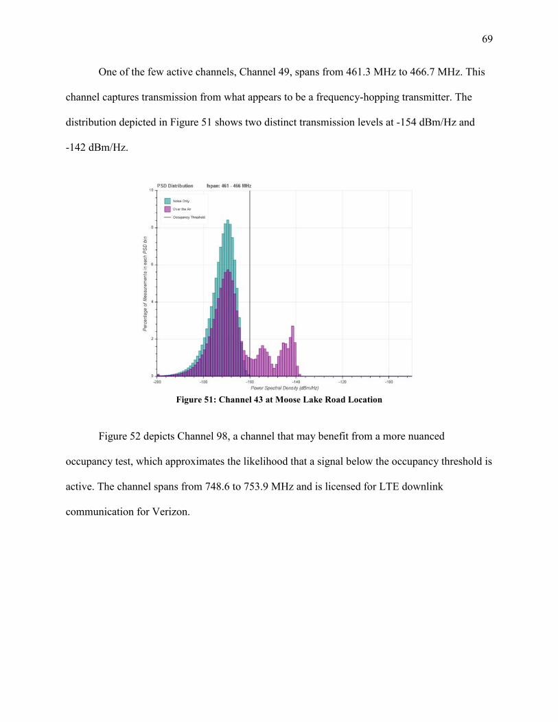
69

One of the few active channels, Channel 49, spans from 461.3 MHz to 466.7 MHz. This

channel captures transmission from what appears to be a frequency-hopping transmitter. The

distribution depicted in Figure 51 shows two distinct transmission levels at -154 dBm/Hz and

-142 dBm/Hz.

Figure 51: Channel 43 at Moose Lake Road Location

Figure 52 depicts Channel 98, a channel that may benefit from a more nuanced

occupancy test, which approximates the likelihood that a signal below the occupancy threshold is

active. The channel spans from 748.6 to 753.9 MHz and is licensed for LTE downlink

communication for Verizon.

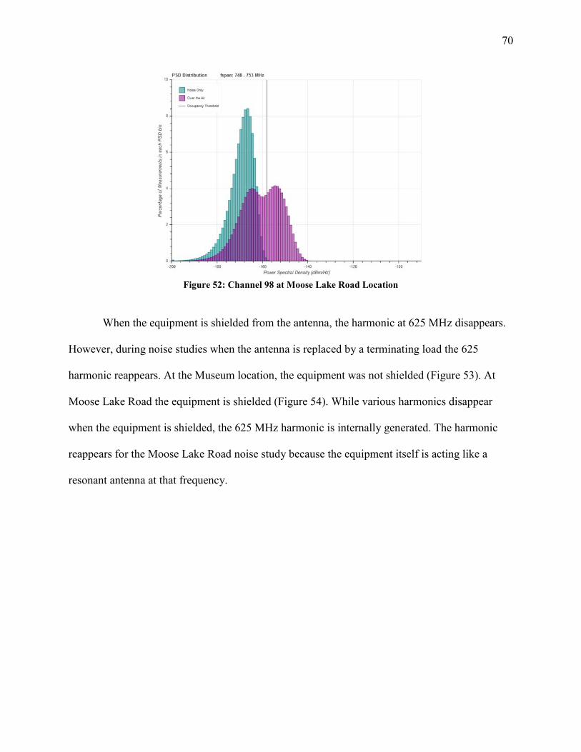
70

Figure 52: Channel 98 at Moose Lake Road Location

When the equipment is shielded from the antenna, the harmonic at 625 MHz disappears.

However, during noise studies when the antenna is replaced by a terminating load the 625

harmonic reappears. At the Museum location, the equipment was not shielded (Figure 53). At

Moose Lake Road the equipment is shielded (Figure 54). While various harmonics disappear

when the equipment is shielded, the 625 MHz harmonic is internally generated. The harmonic

reappears for the Moose Lake Road noise study because the equipment itself is acting like a

resonant antenna at that frequency.

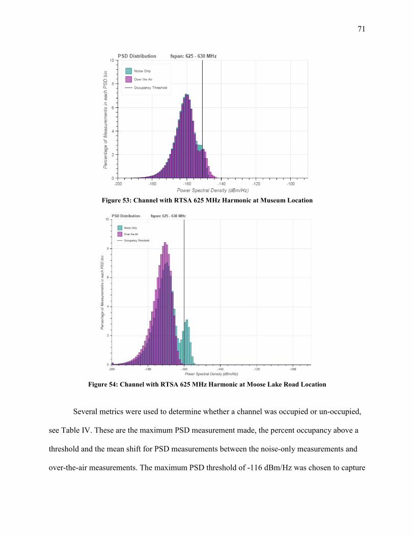
71

Figure 53: Channel with RTSA 625 MHz Harmonic at Museum Location

Figure 54: Channel with RTSA 625 MHz Harmonic at Moose Lake Road Location

Several metrics were used to determine whether a channel was occupied or un-occupied,

see Table IV. These are the maximum PSD measurement made, the percent occupancy above a

threshold and the mean shift for PSD measurements between the noise-only measurements and

over-the-air measurements. The maximum PSD threshold of -116 dBm/Hz was chosen to capture

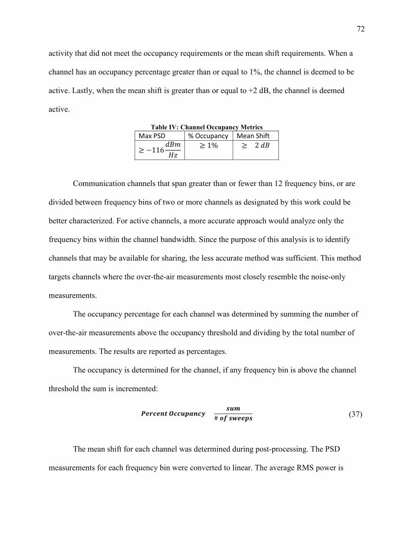
72

activity that did not meet the occupancy requirements or the mean shift requirements. When a

channel has an occupancy percentage greater than or equal to 1%, the channel is deemed to be

active. Lastly, when the mean shift is greater than or equal to +2 dB, the channel is deemed

active.

Table IV: Channel Occupancy Metrics Max PSD % Occupancy Mean Shift

≥ −116𝑑𝑑𝑑𝑑𝑑𝑑𝑀𝑀𝑀𝑀

≥ 1% ≥ +2 𝑑𝑑𝑑𝑑

Communication channels that span greater than or fewer than 12 frequency bins, or are

divided between frequency bins of two or more channels as designated by this work could be

better characterized. For active channels, a more accurate approach would analyze only the

frequency bins within the channel bandwidth. Since the purpose of this analysis is to identify

channels that may be available for sharing, the less accurate method was sufficient. This method

targets channels where the over-the-air measurements most closely resemble the noise-only

measurements.

The occupancy percentage for each channel was determined by summing the number of

over-the-air measurements above the occupancy threshold and dividing by the total number of

measurements. The results are reported as percentages.

The occupancy is determined for the channel, if any frequency bin is above the channel

threshold the sum is incremented:

𝑷𝑷𝒃𝒃𝒍𝒍𝒄𝒄𝒃𝒃𝒃𝒃𝒕𝒕 𝑳𝑳𝒄𝒄𝒄𝒄𝒎𝒎𝒑𝒑𝒃𝒃𝒃𝒃𝒄𝒄𝒚𝒚 =𝑵𝑵𝒎𝒎𝒎𝒎

# 𝒎𝒎𝟐𝟐 𝑵𝑵𝒃𝒃𝒃𝒃𝒃𝒃𝒑𝒑𝑵𝑵 (37)

The mean shift for each channel was determined during post-processing. The PSD

measurements for each frequency bin were converted to linear. The average RMS power is

73

determined by summing the linear channel power of each sweep, and finding the average. The

linear average result is then converted to decibel:

𝑷𝑷𝒍𝒍𝒎𝒎𝑵𝑵 =𝟏𝟏𝒃𝒃�𝑷𝑷𝑬𝑬𝑻𝑻,𝒎𝒎𝒃𝒃𝒃𝒃𝒃𝒃𝒃𝒃𝒍𝒍 ,𝒃𝒃 = # 𝒎𝒎𝟐𝟐 𝑵𝑵𝒃𝒃𝒃𝒃𝒃𝒃𝒑𝒑𝑵𝑵 (38)

The difference was found between the RMS power of over-the-air measurement and the

noise only measurements. A positive-shift occurs when the mean of the over-the-air

measurements is greater than the mean of the noise-only measurements.

As a consequence of these three metrics, there are 71 Channels for the Museum location,

and 14 channels for the Moose Lake Road location that are designated occupied. See Appendix

C for a table of occupied channels at the Montana Tech Museum location and Table V for a

occupied channels at the Moose Lake Road location. These tables are divided into bands that

share the same spectrum allocation as found on SpectrumWiki.com [58]. The FCC TV channel

database was used to identify TV broadcast transmissions in Montana [59].

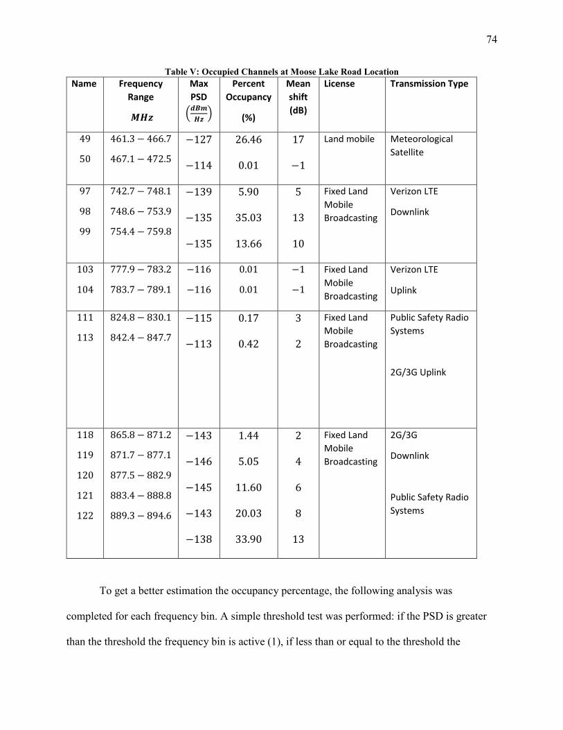
74

Table V: Occupied Channels at Moose Lake Road Location Name Frequency

Range

(𝑴𝑴𝑯𝑯𝑯𝑯)

Max PSD

�𝒃𝒃𝒅𝒅𝒎𝒎𝑯𝑯𝑯𝑯

�

Percent Occupancy

(%)

Mean shift (dB)

License

Transmission Type

49

50

461.3− 466.7

467.1 − 472.5

−127

−114

26.46

0.01

17

−1

Land mobile Meteorological Satellite

97

98

99

742.7− 748.1

748.6− 753.9

754.4− 759.8

−139

−135

−135

5.90

35.03

13.66

5

13

10

Fixed Land Mobile Broadcasting

Verizon LTE

Downlink

103

104

777.9− 783.2

783.7− 789.1

−116

−116

0.01

0.01

−1

−1

Fixed Land Mobile Broadcasting

Verizon LTE

Uplink

111

113

824.8 − 830.1

842.4− 847.7

−115

−113

0.17

0.42

3

2

Fixed Land Mobile Broadcasting

Public Safety Radio Systems

2G/3G Uplink

118

119

120

121

122

865.8 − 871.2

871.7− 877.1

877.5− 882.9

883.4− 888.8

889.3− 894.6

−143

−146

−145

−143

−138

1.44

5.05

11.60

20.03

33.90

2

4

6

8

13

Fixed Land Mobile Broadcasting

2G/3G

Downlink

Public Safety Radio Systems

To get a better estimation the occupancy percentage, the following analysis was

completed for each frequency bin. A simple threshold test was performed: if the PSD is greater

than the threshold the frequency bin is active (1), if less than or equal to the threshold the

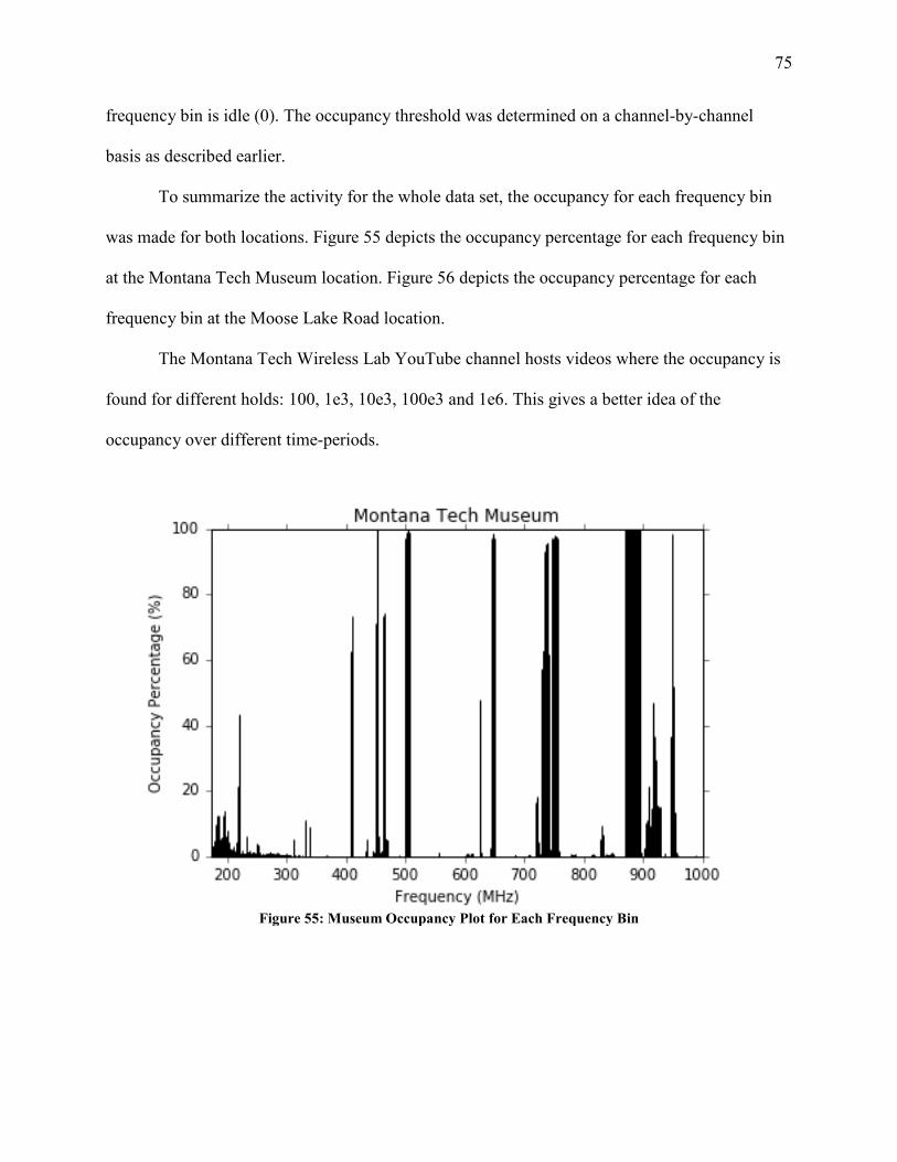
75

frequency bin is idle (0). The occupancy threshold was determined on a channel-by-channel

basis as described earlier.

To summarize the activity for the whole data set, the occupancy for each frequency bin

was made for both locations. Figure 55 depicts the occupancy percentage for each frequency bin

at the Montana Tech Museum location. Figure 56 depicts the occupancy percentage for each

frequency bin at the Moose Lake Road location.

The Montana Tech Wireless Lab YouTube channel hosts videos where the occupancy is

found for different holds: 100, 1e3, 10e3, 100e3 and 1e6. This gives a better idea of the

occupancy over different time-periods.

Figure 55: Museum Occupancy Plot for Each Frequency Bin

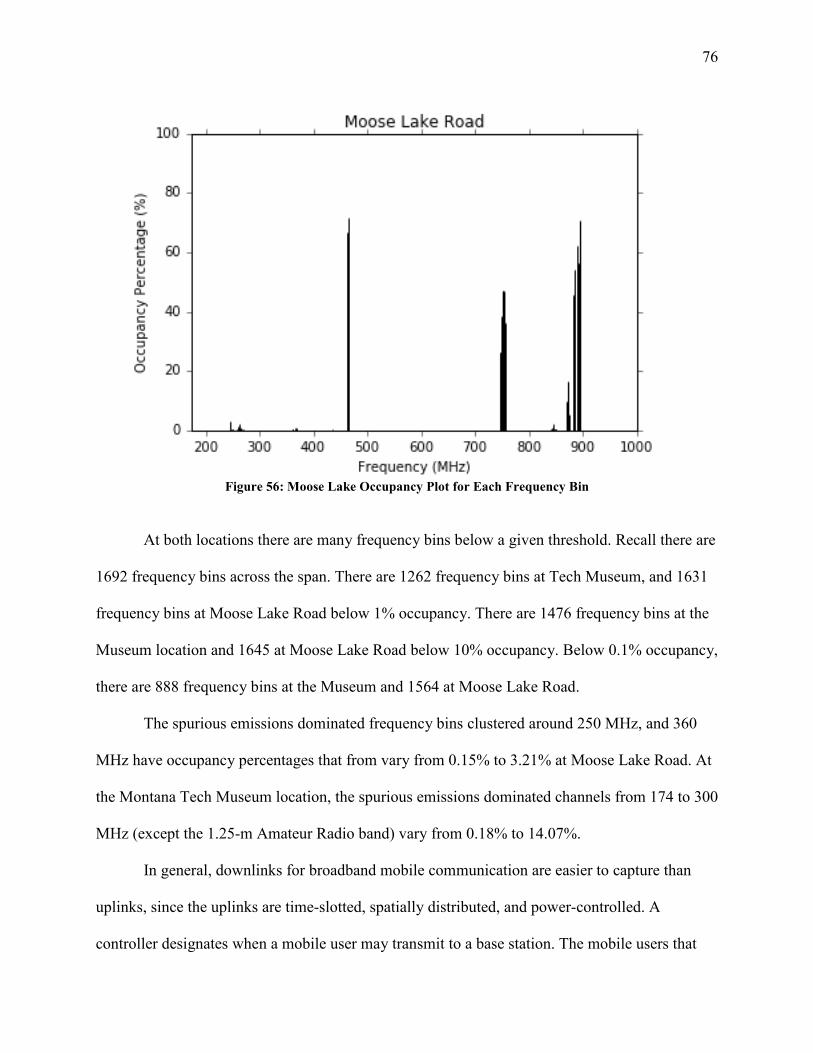
76

Figure 56: Moose Lake Occupancy Plot for Each Frequency Bin

At both locations there are many frequency bins below a given threshold. Recall there are

1692 frequency bins across the span. There are 1262 frequency bins at Tech Museum, and 1631

frequency bins at Moose Lake Road below 1% occupancy. There are 1476 frequency bins at the

Museum location and 1645 at Moose Lake Road below 10% occupancy. Below 0.1% occupancy,

there are 888 frequency bins at the Museum and 1564 at Moose Lake Road.

The spurious emissions dominated frequency bins clustered around 250 MHz, and 360

MHz have occupancy percentages that from vary from 0.15% to 3.21% at Moose Lake Road. At

the Montana Tech Museum location, the spurious emissions dominated channels from 174 to 300

MHz (except the 1.25-m Amateur Radio band) vary from 0.18% to 14.07%.

In general, downlinks for broadband mobile communication are easier to capture than

uplinks, since the uplinks are time-slotted, spatially distributed, and power-controlled. A

controller designates when a mobile user may transmit to a base station. The mobile users that

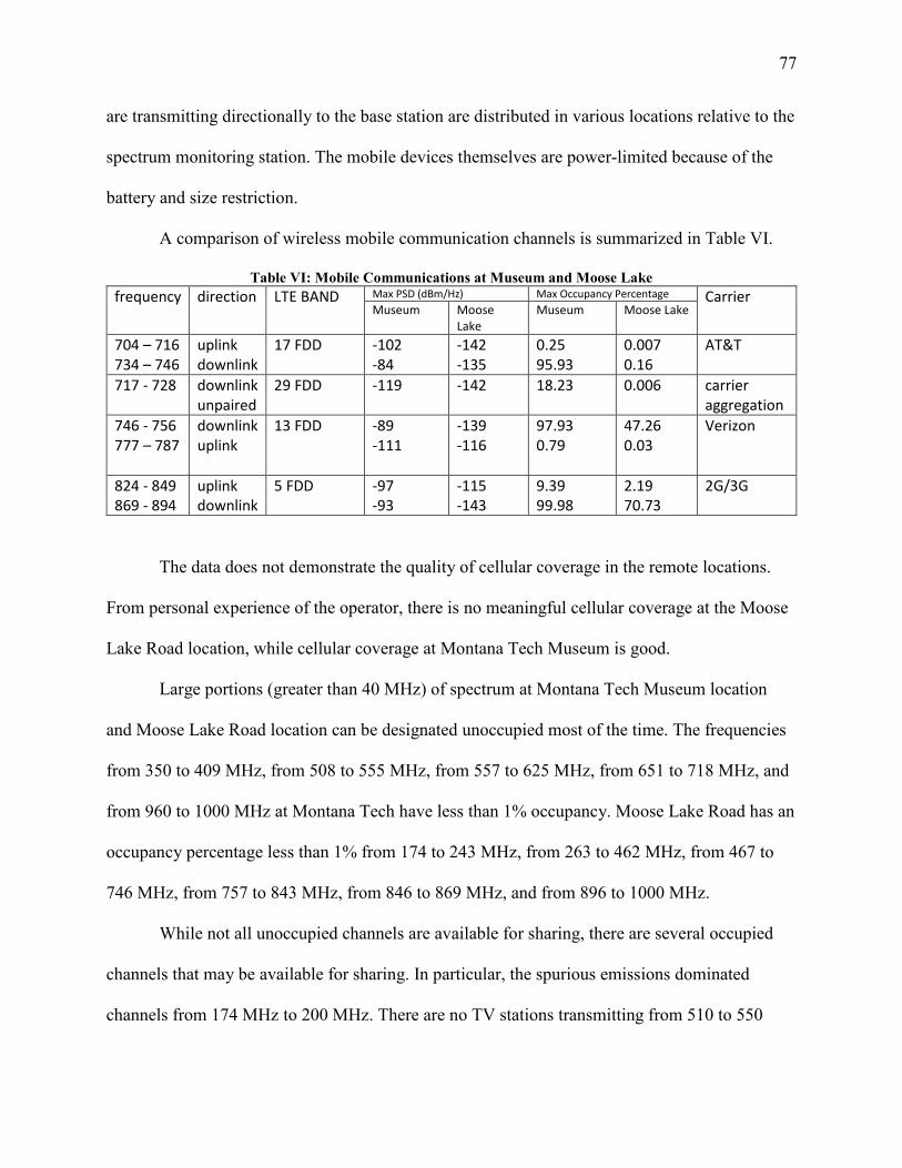
77

are transmitting directionally to the base station are distributed in various locations relative to the

spectrum monitoring station. The mobile devices themselves are power-limited because of the

battery and size restriction.

A comparison of wireless mobile communication channels is summarized in Table VI.

Table VI: Mobile Communications at Museum and Moose Lake frequency direction LTE BAND Max PSD (dBm/Hz) Max Occupancy Percentage Carrier

Museum Moose Lake

Museum Moose Lake

704 – 716 734 – 746

uplink downlink

17 FDD -102 -84

-142 -135

0.25 95.93

0.007 0.16

AT&T

717 - 728 downlink unpaired

29 FDD -119 -142 18.23 0.006 carrier aggregation

746 - 756 777 – 787

downlink uplink

13 FDD -89 -111

-139 -116

97.93 0.79

47.26 0.03

Verizon

824 - 849 869 - 894

uplink downlink

5 FDD -97 -93

-115 -143

9.39 99.98

2.19 70.73

2G/3G

The data does not demonstrate the quality of cellular coverage in the remote locations.

From personal experience of the operator, there is no meaningful cellular coverage at the Moose

Lake Road location, while cellular coverage at Montana Tech Museum is good.

Large portions (greater than 40 MHz) of spectrum at Montana Tech Museum location

and Moose Lake Road location can be designated unoccupied most of the time. The frequencies

from 350 to 409 MHz, from 508 to 555 MHz, from 557 to 625 MHz, from 651 to 718 MHz, and

from 960 to 1000 MHz at Montana Tech have less than 1% occupancy. Moose Lake Road has an

occupancy percentage less than 1% from 174 to 243 MHz, from 263 to 462 MHz, from 467 to

746 MHz, from 757 to 843 MHz, from 846 to 869 MHz, and from 896 to 1000 MHz.

While not all unoccupied channels are available for sharing, there are several occupied

channels that may be available for sharing. In particular, the spurious emissions dominated

channels from 174 MHz to 200 MHz. There are no TV stations transmitting from 510 to 550

78

MHz in the Butte-Silver Bow County where Montana Tech is located, or in Granite County

where Moose Lake Road is located. While some of these channels are dominated by spurious

emissions in Butte, they are relatively free of any transmission at Moose Lake Road. Even

though the frequencies from 902 to 928 MHz are designated “occupied” at the Montana Tech

locations and are allocated for unlicensed ISM use.

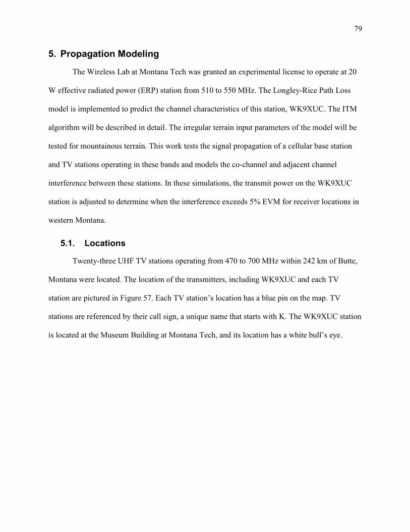
79

5. Propagation Modeling

The Wireless Lab at Montana Tech was granted an experimental license to operate at 20

W effective radiated power (ERP) station from 510 to 550 MHz. The Longley-Rice Path Loss

model is implemented to predict the channel characteristics of this station, WK9XUC. The ITM

algorithm will be described in detail. The irregular terrain input parameters of the model will be

tested for mountainous terrain. This work tests the signal propagation of a cellular base station

and TV stations operating in these bands and models the co-channel and adjacent channel

interference between these stations. In these simulations, the transmit power on the WK9XUC

station is adjusted to determine when the interference exceeds 5% EVM for receiver locations in

western Montana.

5.1. Locations

Twenty-three UHF TV stations operating from 470 to 700 MHz within 242 km of Butte,

Montana were located. The location of the transmitters, including WK9XUC and each TV

station are pictured in Figure 57. Each TV station’s location has a blue pin on the map. TV

stations are referenced by their call sign, a unique name that starts with K. The WK9XUC station

is located at the Museum Building at Montana Tech, and its location has a white bull’s eye.

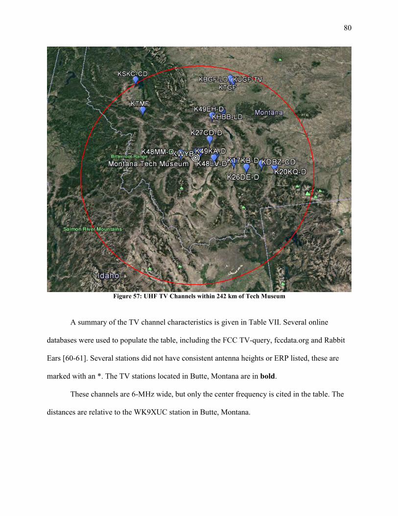
80

Figure 57: UHF TV Channels within 242 km of Tech Museum

A summary of the TV channel characteristics is given in Table VII. Several online

databases were used to populate the table, including the FCC TV-query, fccdata.org and Rabbit

Ears [60-61]. Several stations did not have consistent antenna heights or ERP listed, these are

marked with an *. The TV stations located in Butte, Montana are in bold.

These channels are 6-MHz wide, but only the center frequency is cited in the table. The

distances are relative to the WK9XUC station in Butte, Montana.

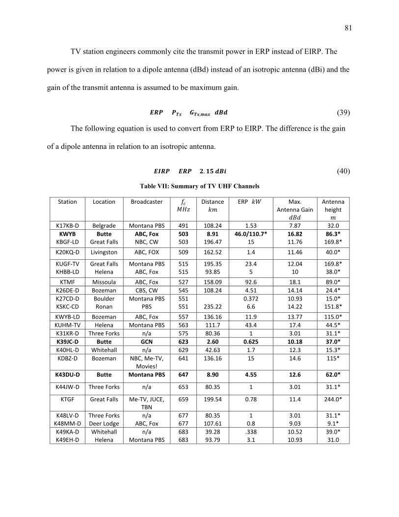
81

TV station engineers commonly cite the transmit power in ERP instead of EIRP. The

power is given in relation to a dipole antenna (dBd) instead of an isotropic antenna (dBi) and the

gain of the transmit antenna is assumed to be maximum gain.

𝑬𝑬𝑬𝑬𝑷𝑷 = 𝑷𝑷𝑻𝑻𝑻𝑻 + 𝑮𝑮𝑻𝑻𝑻𝑻,𝒎𝒎𝒃𝒃𝑻𝑻 (𝒃𝒃𝒅𝒅𝒃𝒃) (39)

The following equation is used to convert from ERP to EIRP. The difference is the gain

of a dipole antenna in relation to an isotropic antenna.

𝑬𝑬𝑬𝑬𝑬𝑬𝑷𝑷 = 𝑬𝑬𝑬𝑬𝑷𝑷 + 𝟐𝟐.𝟏𝟏𝟐𝟐 𝒃𝒃𝒅𝒅𝒃𝒃 (40)

Table VII: Summary of TV UHF Channels

Station Location Broadcaster 𝑓𝑓𝑐𝑐 [𝐼𝐼𝑀𝑀𝑀𝑀]

Distance [𝑘𝑘𝑑𝑑]

ERP [𝑘𝑘𝑘𝑘] Max. Antenna Gain

[𝑑𝑑𝑑𝑑𝑑𝑑]

Antenna height

[𝑑𝑑] K17KB-D Belgrade Montana PBS 491 108.24 1.53 7.87 32.0

KWYB KBGF-LD

Butte Great Falls

ABC, Fox NBC, CW

503 503

8.91 196.47

46.0/110.7* 15

16.82 11.76

86.3* 169.8*

K20KQ-D Livingston ABC, FOX 509 162.52 1.4 11.46 40.0*

KUGF-TV KHBB-LD

Great Falls Helena

Montana PBS ABC, Fox

515 515

195.35 93.85

23.4 5

12.04 10

169.8* 38.0*

KTMF Missoula ABC, Fox 527 158.09 92.6 18.1 89.0* K26DE-D Bozeman CBS, CW 545 108.24 4.51 14.14 24.4* K27CD-D KSKC-CD

Boulder Ronan

Montana PBS PBS

551 551

235.22

0.372 6.6

10.93 14.22

15.0* 151.8*

KWYB-LD Bozeman ABC, Fox 557 136.16 11.9 13.77 115.0* KUHM-TV Helena Montana PBS 563 111.7 43.4 17.4 44.5* K31KR-D Three Forks n/a 575 80.36 1 3.01 31.1* K39JC-D Butte GCN 623 2.60 0.625 10.18 37.0* K40HL-D Whitehall n/a 629 42.63 1.7 12.3 15.3* KDBZ-D Bozeman NBC, Me-TV,

Movies! 641 136.16 15 14.6 115*

K43DU-D Butte Montana PBS 647 8.90 4.55 12.6 62.0*

K44JW-D Three Forks n/a 653 80.35 1 3.01 31.1*

KTGF Great Falls Me-TV, JUCE, TBN

659 199.54 0.78 11.4 244.0*

K48LV-D K48MM-D

Three Forks Deer Lodge

n/a ABC, Fox

677 677

80.35 107.61

1 0.8

3.01 9.03

31.1* 9.1*

K49KA-D K49EH-D

Whitehall Helena

n/a Montana PBS

683 683

39.28 93.79

.338 3.1

10.52 10.93

39.0* 31.0

82

KWYB’s license to operate at a lower power level is temporary due to damage to the

transmitter equipment. When channel measurements were performed in August/September 2016

the antenna was transmitting at the lower power. This station is expected to be repaired in spring

or summer of 2017. For measurement results, the transmit power is lower, EIRP of 79 dBm, for

predictive results, both power levels will be presented. The higher transmit power is 83 dBm.

To predict the channel characteristics of this lab’s station WK9XUC, SPLAT! was used

to model the path loss to a grid of receiver sites in Butte and population centers within 50 km of

Butte, specifically Anaconda, Deer Lodge, Boulder, Whitehall, Cardwell, and Divide. Figure 58

depicts the relative locations. Each population grid contained Rx sites spaced 1 km apart. All

receiver locations in the population grid have a height of 6 meter. Furthermore, each grid was

defined by a set of latitudes and longitudes: (N, E), (S, E), (S, W), and (N, W). The

characteristics of each grid is summarized in Table VIII.

Since a large set of path loss predictions were required for this work and SPLAT! is used

from the command line, various bash scripts were employed (see Appendix D for more details).

The average path loss was found for WK9XUC operating at 500 MHz and 560 MHz. For most

locations, the maximum difference was 3 dB and the average difference was 2 dB. The path loss

is used to determine the received channel power for each Rx location on the grid. The SNR was

determined for the TV stations, and the SINR was determined by adjusting the power level of

WK9XUC.

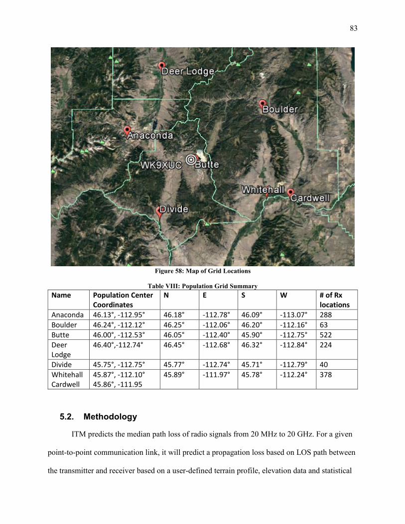
83

Figure 58: Map of Grid Locations

Table VIII: Population Grid Summary

Name Population Center Coordinates

N E S W # of Rx locations

Anaconda 46.13°, -112.95° 46.18° -112.78° 46.09° -113.07° 288 Boulder 46.24°, -112.12° 46.25° -112.06° 46.20° -112.16° 63 Butte 46.00°, -112.53° 46.05° -112.40° 45.90° -112.75° 522 Deer Lodge

46.40°,-112.74° 46.45° -112.68° 46.32° -112.84° 224

Divide 45.75°, -112.75° 45.77° -112.74° 45.71° -112.79° 40 Whitehall Cardwell

45.87°, -112.10° 45.86°, -111.95

45.89° -111.97° 45.78° -112.24° 378

5.2. Methodology

ITM predicts the median path loss of radio signals from 20 MHz to 20 GHz. For a given

point-to-point communication link, it will predict a propagation loss based on LOS path between

the transmitter and receiver based on a user-defined terrain profile, elevation data and statistical

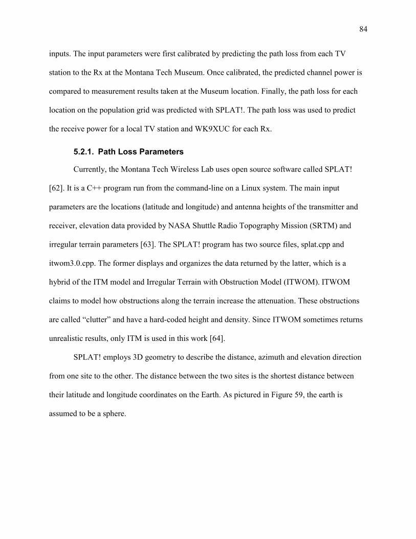
84

inputs. The input parameters were first calibrated by predicting the path loss from each TV

station to the Rx at the Montana Tech Museum. Once calibrated, the predicted channel power is

compared to measurement results taken at the Museum location. Finally, the path loss for each

location on the population grid was predicted with SPLAT!. The path loss was used to predict

the receive power for a local TV station and WK9XUC for each Rx.

5.2.1. Path Loss Parameters

Currently, the Montana Tech Wireless Lab uses open source software called SPLAT!

[62]. It is a C++ program run from the command-line on a Linux system. The main input

parameters are the locations (latitude and longitude) and antenna heights of the transmitter and

receiver, elevation data provided by NASA Shuttle Radio Topography Mission (SRTM) and

irregular terrain parameters [63]. The SPLAT! program has two source files, splat.cpp and

itwom3.0.cpp. The former displays and organizes the data returned by the latter, which is a

hybrid of the ITM model and Irregular Terrain with Obstruction Model (ITWOM). ITWOM

claims to model how obstructions along the terrain increase the attenuation. These obstructions

are called “clutter” and have a hard-coded height and density. Since ITWOM sometimes returns

unrealistic results, only ITM is used in this work [64].

SPLAT! employs 3D geometry to describe the distance, azimuth and elevation direction

from one site to the other. The distance between the two sites is the shortest distance between

their latitude and longitude coordinates on the Earth. As pictured in Figure 59, the earth is

assumed to be a sphere.

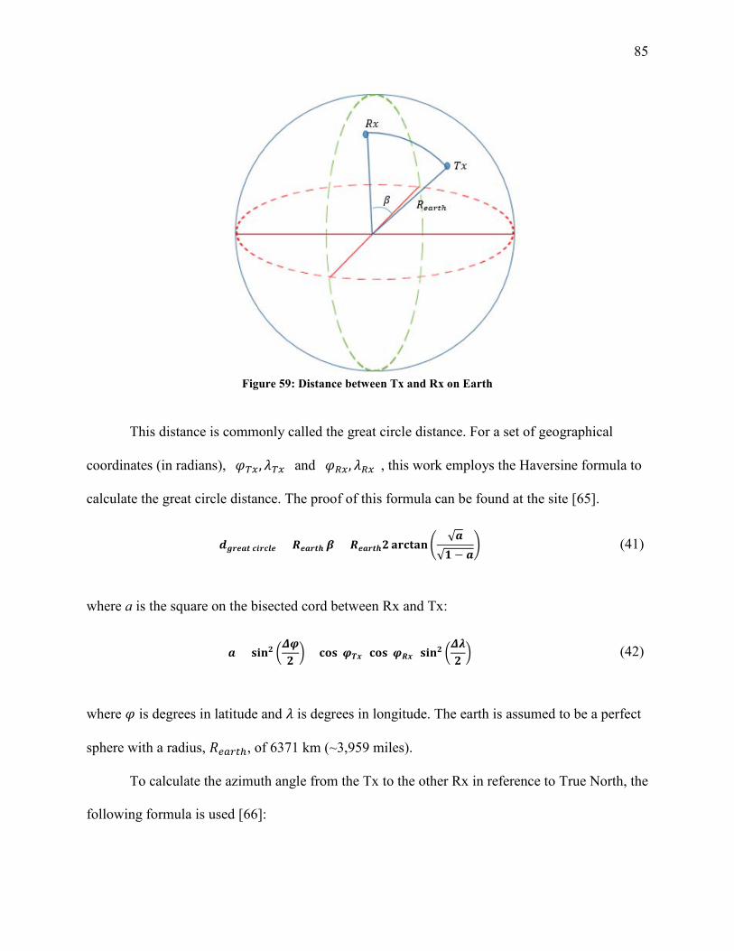
85

Figure 59: Distance between Tx and Rx on Earth

This distance is commonly called the great circle distance. For a set of geographical

coordinates (in radians), (𝜑𝜑𝑇𝑇𝑇𝑇,𝜆𝜆𝑇𝑇𝑇𝑇) and (𝜑𝜑𝑅𝑅𝑇𝑇, 𝜆𝜆𝑅𝑅𝑇𝑇), this work employs the Haversine formula to

calculate the great circle distance. The proof of this formula can be found at the site [65].

𝒃𝒃𝒈𝒈𝒍𝒍𝒃𝒃𝒃𝒃𝒕𝒕 𝒄𝒄𝒃𝒃𝒍𝒍𝒄𝒄𝒎𝒎𝒃𝒃 = 𝑬𝑬𝒃𝒃𝒃𝒃𝒍𝒍𝒕𝒕𝒃𝒃 𝜷𝜷 = 𝑬𝑬𝒃𝒃𝒃𝒃𝒍𝒍𝒕𝒕𝒃𝒃𝟐𝟐 𝐚𝐚𝐚𝐚𝐜𝐜𝐚𝐚𝐚𝐚𝐚𝐚�√𝒃𝒃

√𝟏𝟏 − 𝒃𝒃� (41)

where a is the square on the bisected cord between Rx and Tx:

𝒃𝒃 = 𝐜𝐜𝐬𝐬𝐚𝐚𝟐𝟐 �𝜟𝜟𝝋𝝋𝟐𝟐� + 𝐜𝐜𝐜𝐜𝐜𝐜(𝝋𝝋𝑻𝑻𝑻𝑻) 𝐜𝐜𝐜𝐜𝐜𝐜(𝝋𝝋𝑬𝑬𝑻𝑻) 𝐜𝐜𝐬𝐬𝐚𝐚𝟐𝟐 �

𝜟𝜟𝝀𝝀𝟐𝟐� (42)

where 𝜑𝜑 is degrees in latitude and 𝜆𝜆 is degrees in longitude. The earth is assumed to be a perfect

sphere with a radius, 𝑅𝑅𝑏𝑏𝑏𝑏𝑙𝑙𝑟𝑟ℎ, of 6371 km (~3,959 miles).

To calculate the azimuth angle from the Tx to the other Rx in reference to True North, the

following formula is used [66]:

86

𝜽𝜽 = 𝟐𝟐𝐚𝐚𝐚𝐚𝐜𝐜𝐚𝐚𝐚𝐚𝐚𝐚�𝐜𝐜𝐬𝐬𝐚𝐚(𝜟𝜟𝝀𝝀) 𝐜𝐜𝐜𝐜𝐜𝐜(𝝋𝝋𝑬𝑬𝑻𝑻)

𝐜𝐜𝐜𝐜𝐜𝐜(𝝋𝝋𝑻𝑻𝑻𝑻) 𝐜𝐜𝐬𝐬𝐚𝐚(𝝋𝝋𝑬𝑬𝑻𝑻) − 𝐜𝐜𝐜𝐜𝐜𝐜(𝝋𝝋𝑻𝑻𝑻𝑻) 𝐜𝐜𝐜𝐜𝐜𝐜(𝝋𝝋𝑬𝑬𝑻𝑻) 𝐜𝐜𝐜𝐜𝐜𝐜(𝜟𝜟𝝀𝝀)� (43)

To return the result in degrees with a range 0° ≤ 𝜃𝜃 < 360°, convert from radians to degrees,

then add 360° to the result then divide by 360° and return the remainder. To find the azimuth of

the Rx to the Tx, alternate the position of the variables. Or perform the following operation, add

180° to the azimuth of the receiver, then divide by 360°, and return the remainder. In Python,

these operations take two lines as pictured in Figure 60:

Figure 60: Python Azimuth Normalization

These equations (Equations 41 – 43) were also used to verify SPLAT! and create the population

grids.

All SRTM elevation files have a raster size of 1° in longitude and latitude but the spatial

resolution varies. The spatial resolution or distance between each elevation sample depends on

the latitude and whether the file is either SRTM3 or SRTM1. All elevations are given to the

nearest meter. Figure 61 and Figure 62 depict the coverage area across the globe from SRTM1

and SRTM3 respectively [67, 68]. Path Loss analysis performed with SRTM1 is designated HD,

and with SRTM3 non-HD.

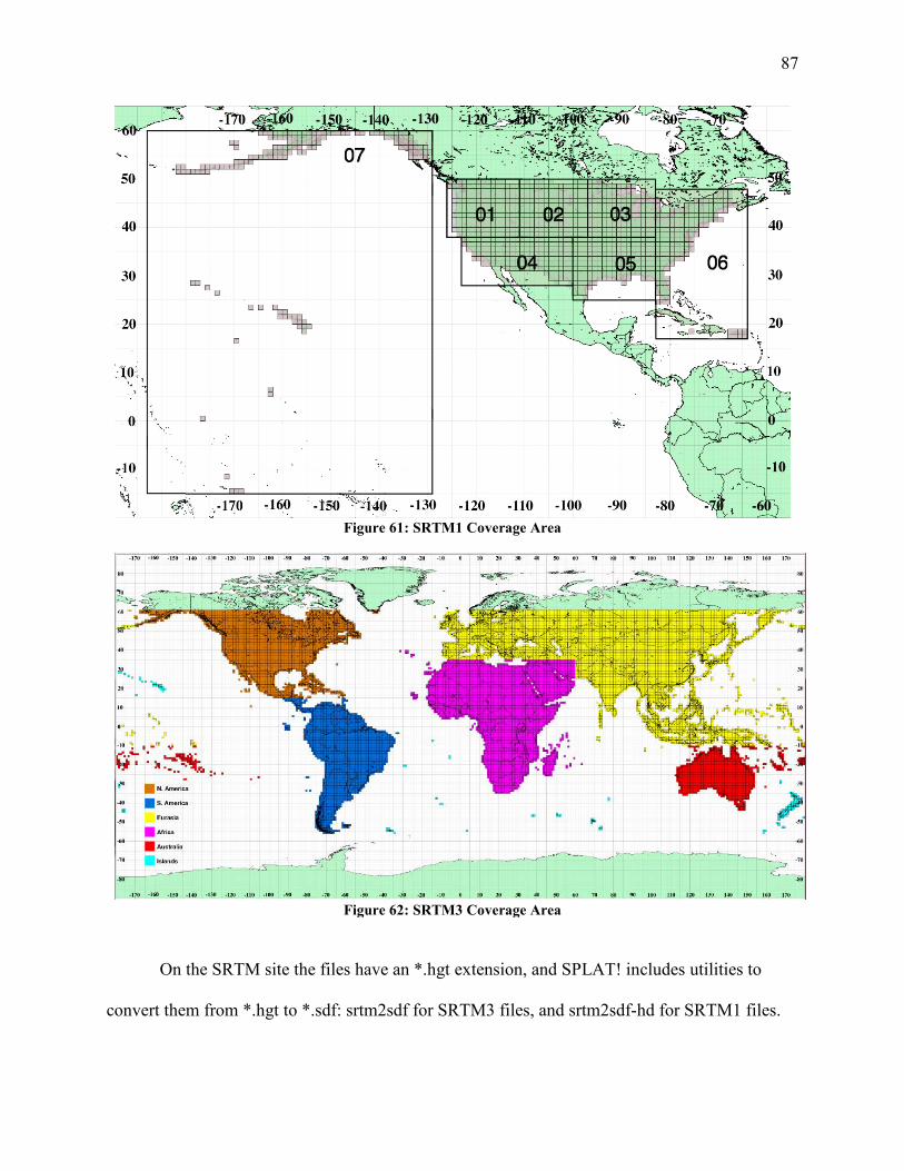
87

Figure 61: SRTM1 Coverage Area

Figure 62: SRTM3 Coverage Area

On the SRTM site the files have an *.hgt extension, and SPLAT! includes utilities to

convert them from *.hgt to *.sdf: srtm2sdf for SRTM3 files, and srtm2sdf-hd for SRTM1 files.

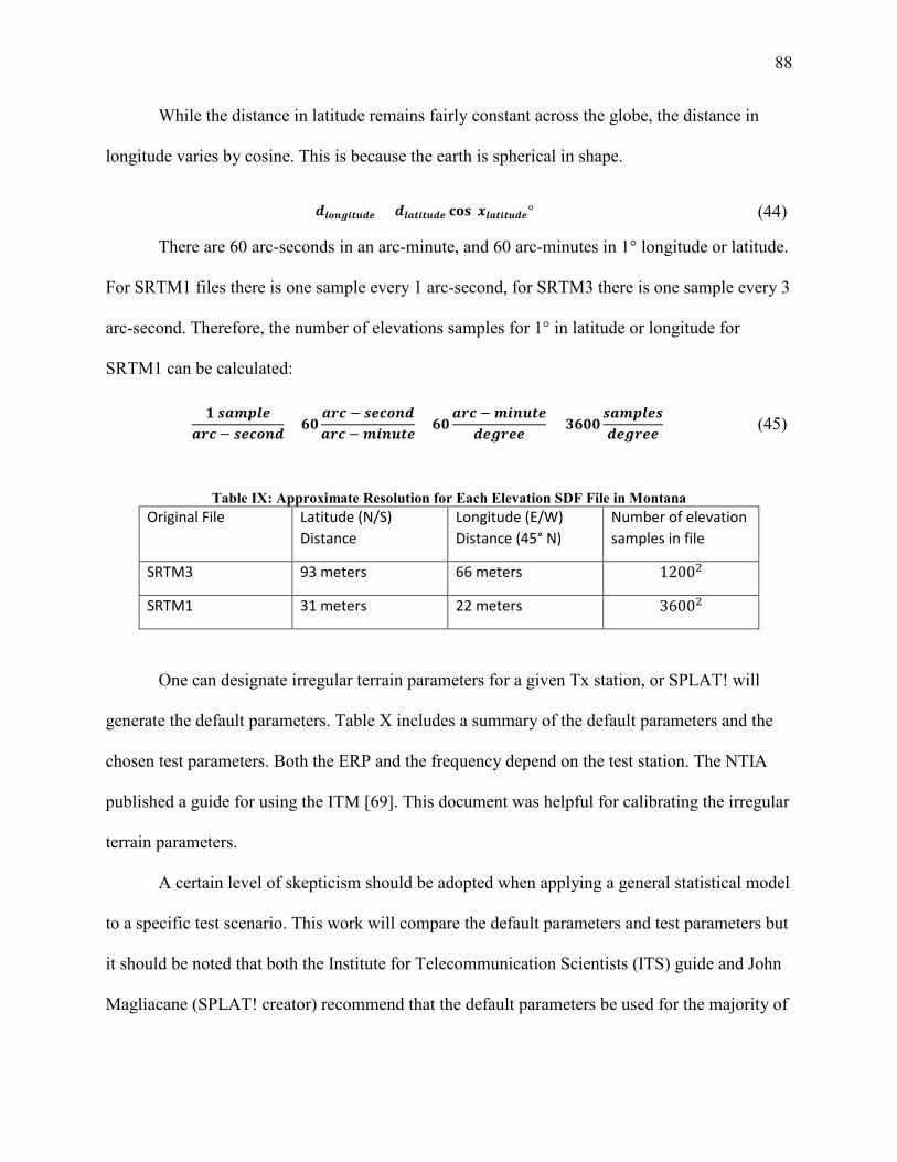
88

While the distance in latitude remains fairly constant across the globe, the distance in

longitude varies by cosine. This is because the earth is spherical in shape.

𝒃𝒃𝒎𝒎𝒎𝒎𝒃𝒃𝒈𝒈𝒃𝒃𝒕𝒕𝒎𝒎𝒃𝒃𝒃𝒃 = 𝒃𝒃𝒎𝒎𝒃𝒃𝒕𝒕𝒃𝒃𝒕𝒕𝒎𝒎𝒃𝒃𝒃𝒃 𝐜𝐜𝐜𝐜𝐜𝐜(𝑻𝑻𝒎𝒎𝒃𝒃𝒕𝒕𝒃𝒃𝒕𝒕𝒎𝒎𝒃𝒃𝒃𝒃°) (44)

There are 60 arc-seconds in an arc-minute, and 60 arc-minutes in 1° longitude or latitude.

For SRTM1 files there is one sample every 1 arc-second, for SRTM3 there is one sample every 3

arc-second. Therefore, the number of elevations samples for 1° in latitude or longitude for

SRTM1 can be calculated:

𝟏𝟏 𝑵𝑵𝒃𝒃𝒎𝒎𝒑𝒑𝒎𝒎𝒃𝒃𝒃𝒃𝒍𝒍𝒄𝒄 − 𝑵𝑵𝒃𝒃𝒄𝒄𝒎𝒎𝒃𝒃𝒃𝒃

× 𝟔𝟔𝟏𝟏𝒃𝒃𝒍𝒍𝒄𝒄 − 𝑵𝑵𝒃𝒃𝒄𝒄𝒎𝒎𝒃𝒃𝒃𝒃𝒃𝒃𝒍𝒍𝒄𝒄 −𝒎𝒎𝒃𝒃𝒃𝒃𝒎𝒎𝒕𝒕𝒃𝒃

× 𝟔𝟔𝟏𝟏𝒃𝒃𝒍𝒍𝒄𝒄 −𝒎𝒎𝒃𝒃𝒃𝒃𝒎𝒎𝒕𝒕𝒃𝒃

𝒃𝒃𝒃𝒃𝒈𝒈𝒍𝒍𝒃𝒃𝒃𝒃= 𝟑𝟑𝟔𝟔𝟏𝟏𝟏𝟏

𝑵𝑵𝒃𝒃𝒎𝒎𝒑𝒑𝒎𝒎𝒃𝒃𝑵𝑵𝒃𝒃𝒃𝒃𝒈𝒈𝒍𝒍𝒃𝒃𝒃𝒃

(45)

Table IX: Approximate Resolution for Each Elevation SDF File in Montana Original File Latitude (N/S)

Distance Longitude (E/W) Distance (45° N)

Number of elevation samples in file

SRTM3 93 meters 66 meters 12002

SRTM1 31 meters 22 meters 36002

One can designate irregular terrain parameters for a given Tx station, or SPLAT! will

generate the default parameters. Table X includes a summary of the default parameters and the

chosen test parameters. Both the ERP and the frequency depend on the test station. The NTIA

published a guide for using the ITM [69]. This document was helpful for calibrating the irregular

terrain parameters.

A certain level of skepticism should be adopted when applying a general statistical model

to a specific test scenario. This work will compare the default parameters and test parameters but

it should be noted that both the Institute for Telecommunication Scientists (ITS) guide and John

Magliacane (SPLAT! creator) recommend that the default parameters be used for the majority of

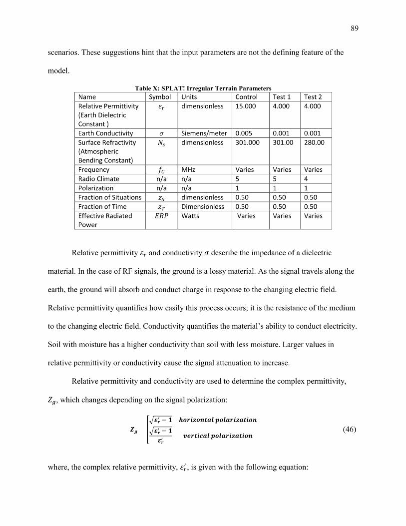
89

scenarios. These suggestions hint that the input parameters are not the defining feature of the

model.

Table X: SPLAT! Irregular Terrain Parameters Name Symbol Units Control Test 1 Test 2 Relative Permittivity (Earth Dielectric Constant )

𝜀𝜀𝑙𝑙 dimensionless 15.000 4.000 4.000

Earth Conductivity 𝜎𝜎 Siemens/meter 0.005 0.001 0.001 Surface Refractivity (Atmospheric Bending Constant)

𝑁𝑁𝑏𝑏 dimensionless 301.000 301.00 280.00

Frequency 𝑓𝑓𝐶𝐶 MHz Varies Varies Varies Radio Climate n/a n/a 5 5 4 Polarization n/a n/a 1 1 1 Fraction of Situations 𝑀𝑀𝑆𝑆 dimensionless 0.50 0.50 0.50 Fraction of Time 𝑀𝑀𝑇𝑇 Dimensionless 0.50 0.50 0.50 Effective Radiated Power

𝐸𝐸𝑅𝑅𝑃𝑃 Watts Varies Varies Varies

Relative permittivity 𝜀𝜀𝑙𝑙 and conductivity 𝜎𝜎 describe the impedance of a dielectric

material. In the case of RF signals, the ground is a lossy material. As the signal travels along the

earth, the ground will absorb and conduct charge in response to the changing electric field.

Relative permittivity quantifies how easily this process occurs; it is the resistance of the medium

to the changing electric field. Conductivity quantifies the material’s ability to conduct electricity.

Soil with moisture has a higher conductivity than soil with less moisture. Larger values in

relative permittivity or conductivity cause the signal attenuation to increase.

Relative permittivity and conductivity are used to determine the complex permittivity,

𝑍𝑍𝑔𝑔, which changes depending on the signal polarization:

𝒁𝒁𝒈𝒈 = ��𝜺𝜺𝒍𝒍′ − 𝟏𝟏 𝒃𝒃𝒎𝒎𝒍𝒍𝒃𝒃𝑯𝑯𝒎𝒎𝒃𝒃𝒕𝒕𝒃𝒃𝒎𝒎 𝒑𝒑𝒎𝒎𝒎𝒎𝒃𝒃𝒍𝒍𝒃𝒃𝑯𝑯𝒃𝒃𝒕𝒕𝒃𝒃𝒎𝒎𝒃𝒃

�𝜺𝜺𝒍𝒍′ − 𝟏𝟏𝜺𝜺𝒍𝒍′

𝒗𝒗𝒃𝒃𝒍𝒍𝒕𝒕𝒃𝒃𝒄𝒄𝒃𝒃𝒎𝒎 𝒑𝒑𝒎𝒎𝒎𝒎𝒃𝒃𝒍𝒍𝒃𝒃𝑯𝑯𝒃𝒃𝒕𝒕𝒃𝒃𝒎𝒎𝒃𝒃 (46)

where, the complex relative permittivity, 𝜀𝜀𝑙𝑙′ , is given with the following equation:

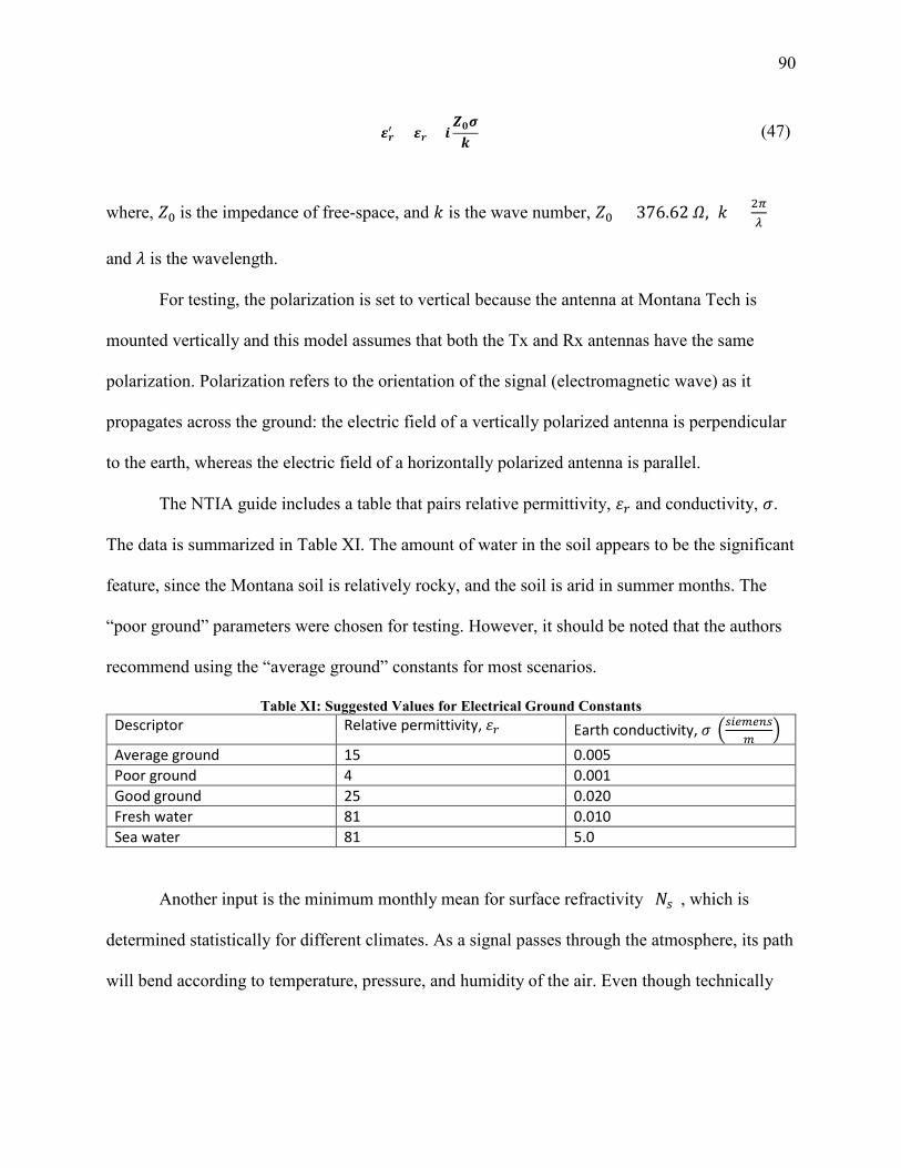
90

𝜺𝜺𝒍𝒍′ = 𝜺𝜺𝒍𝒍 + 𝒃𝒃𝒁𝒁𝟏𝟏𝝈𝝈𝒌𝒌

(47)

where, 𝑍𝑍0 is the impedance of free-space, and 𝑘𝑘 is the wave number, 𝑍𝑍0 = 376.62 𝛺𝛺, 𝑘𝑘 = 2𝜋𝜋𝜆𝜆

and 𝜆𝜆 is the wavelength.

For testing, the polarization is set to vertical because the antenna at Montana Tech is

mounted vertically and this model assumes that both the Tx and Rx antennas have the same

polarization. Polarization refers to the orientation of the signal (electromagnetic wave) as it

propagates across the ground: the electric field of a vertically polarized antenna is perpendicular

to the earth, whereas the electric field of a horizontally polarized antenna is parallel.

The NTIA guide includes a table that pairs relative permittivity, 𝜀𝜀𝑙𝑙 and conductivity, 𝜎𝜎.

The data is summarized in Table XI. The amount of water in the soil appears to be the significant

feature, since the Montana soil is relatively rocky, and the soil is arid in summer months. The

“poor ground” parameters were chosen for testing. However, it should be noted that the authors

recommend using the “average ground” constants for most scenarios.

Table XI: Suggested Values for Electrical Ground Constants Descriptor Relative permittivity, 𝜀𝜀𝑙𝑙 Earth conductivity, 𝜎𝜎 �𝑏𝑏𝑙𝑙𝑏𝑏𝑚𝑚𝑏𝑏𝑏𝑏𝑏𝑏

𝑚𝑚�

Average ground 15 0.005 Poor ground 4 0.001 Good ground 25 0.020 Fresh water 81 0.010 Sea water 81 5.0

Another input is the minimum monthly mean for surface refractivity (𝑁𝑁𝑏𝑏), which is

determined statistically for different climates. As a signal passes through the atmosphere, its path

will bend according to temperature, pressure, and humidity of the air. Even though technically

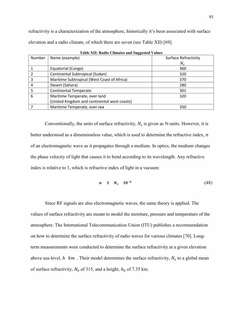
91

refractivity is a characterization of the atmosphere, historically it’s been associated with surface

elevation and a radio climate, of which there are seven (see Table XII) [69].

Table XII: Radio Climates and Suggested Values Number Name (example) Surface Refractivity

𝑁𝑁𝑏𝑏 1 Equatorial (Congo) 360 2 Continental Subtropical (Sudan) 320 3 Maritime Subtropical (West Coast of Africa) 370 4 Desert (Sahara) 280 5 Continental Temperate 301 6 Maritime Temperate, over land

(United Kingdom and continental west coasts) 320

7 Maritime Temperate, over sea 350

Conventionally, the units of surface refractivity, 𝑁𝑁𝑏𝑏 is given as N-units. However, it is

better understood as a dimensionless value, which is used to determine the refractive index, 𝑛𝑛

of an electromagnetic wave as it propagates through a medium. In optics, the medium changes

the phase velocity of light that causes it to bend according to its wavelength. Any refractive

index is relative to 1, which is refractive index of light in a vacuum:

𝒃𝒃 = 𝟏𝟏 + 𝑵𝑵𝑵𝑵 × 𝟏𝟏𝟏𝟏−𝟔𝟔 (48)

Since RF signals are also electromagnetic waves, the same theory is applied. The

values of surface refractivity are meant to model the moisture, pressure and temperature of the

atmosphere. The International Telecommunication Union (ITU) publishes a recommendation

on how to determine the surface refractivity of radio waves for various climates [70]. Long-

term measurements were conducted to determine the surface refractivity at a given elevation

above sea-level, ℎ (𝑘𝑘𝑑𝑑). Their model determines the surface refractivity, 𝑁𝑁𝑏𝑏 to a global mean

of surface refractivity, 𝑁𝑁0 of 315, and a height, ℎ0 of 7.35 km.

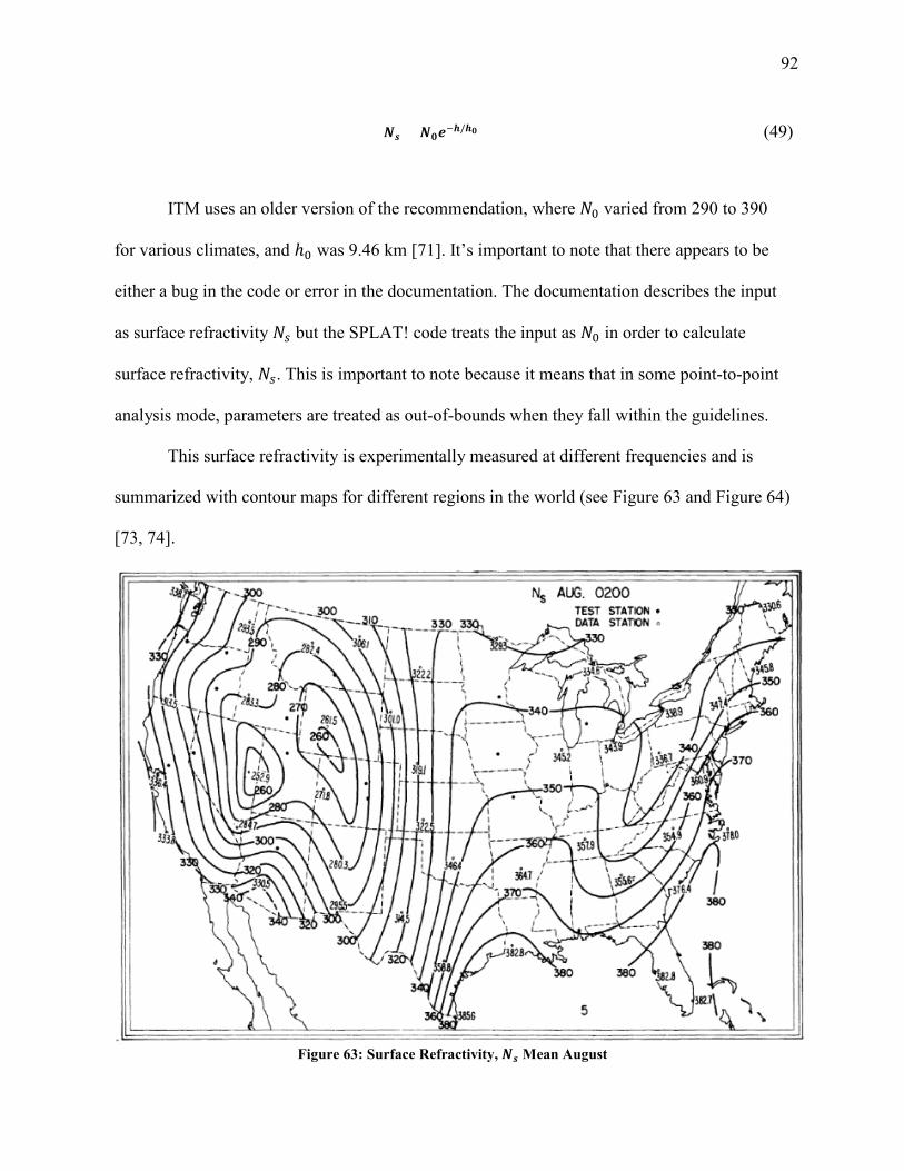
92

𝑵𝑵𝑵𝑵 = 𝑵𝑵𝟏𝟏𝒃𝒃−𝒃𝒃/𝒃𝒃𝟏𝟏 (49)

ITM uses an older version of the recommendation, where 𝑁𝑁0 varied from 290 to 390

for various climates, and ℎ0 was 9.46 km [71]. It’s important to note that there appears to be

either a bug in the code or error in the documentation. The documentation describes the input

as surface refractivity 𝑁𝑁𝑏𝑏 but the SPLAT! code treats the input as 𝑁𝑁0 in order to calculate

surface refractivity, 𝑁𝑁𝑏𝑏. This is important to note because it means that in some point-to-point

analysis mode, parameters are treated as out-of-bounds when they fall within the guidelines.

This surface refractivity is experimentally measured at different frequencies and is

summarized with contour maps for different regions in the world (see Figure 63 and Figure 64)

[73, 74].

Figure 63: Surface Refractivity, 𝑵𝑵𝑵𝑵 Mean August

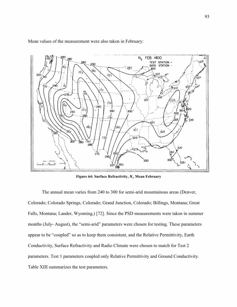
93

Mean values of the measurement were also taken in February:

Figure 64: Surface Refractivity, 𝑵𝑵𝑵𝑵 Mean February

The annual mean varies from 240 to 300 for semi-arid mountainous areas (Denver,

Colorado; Colorado Springs, Colorado; Grand Junction, Colorado; Billings, Montana; Great

Falls, Montana; Lander, Wyoming,) [72]. Since the PSD measurements were taken in summer

months (July- August), the “semi-arid” parameters were chosen for testing. These parameters

appear to be “coupled” so as to keep them consistent, and the Relative Permittivity, Earth

Conductivity, Surface Refractivity and Radio Climate were chosen to match for Test 2

parameters. Test 1 parameters coupled only Relative Permittivity and Ground Conductivity.

Table XIII summarizes the test parameters.

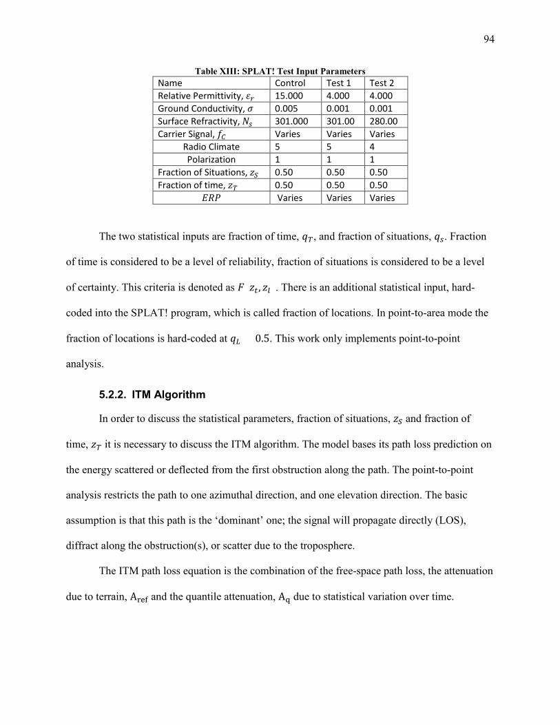
94

Table XIII: SPLAT! Test Input Parameters Name Control Test 1 Test 2 Relative Permittivity, 𝜀𝜀𝑙𝑙 15.000 4.000 4.000 Ground Conductivity, 𝜎𝜎 0.005 0.001 0.001 Surface Refractivity, 𝑁𝑁𝑏𝑏 301.000 301.00 280.00 Carrier Signal, 𝑓𝑓𝐶𝐶 Varies Varies Varies

Radio Climate 5 5 4 Polarization 1 1 1

Fraction of Situations, 𝑀𝑀𝑆𝑆 0.50 0.50 0.50 Fraction of time, 𝑀𝑀𝑇𝑇 0.50 0.50 0.50

𝐸𝐸𝑅𝑅𝑃𝑃 Varies Varies Varies

The two statistical inputs are fraction of time, 𝑞𝑞𝑇𝑇, and fraction of situations, 𝑞𝑞𝑏𝑏. Fraction

of time is considered to be a level of reliability, fraction of situations is considered to be a level

of certainty. This criteria is denoted as 𝑁𝑁(𝑀𝑀𝑟𝑟, 𝑀𝑀𝑙𝑙). There is an additional statistical input, hard-

coded into the SPLAT! program, which is called fraction of locations. In point-to-area mode the

fraction of locations is hard-coded at 𝑞𝑞𝐿𝐿 = 0.5. This work only implements point-to-point

analysis.

5.2.2. ITM Algorithm

In order to discuss the statistical parameters, fraction of situations, 𝑀𝑀𝑆𝑆 and fraction of

time, 𝑀𝑀𝑇𝑇 it is necessary to discuss the ITM algorithm. The model bases its path loss prediction on

the energy scattered or deflected from the first obstruction along the path. The point-to-point

analysis restricts the path to one azimuthal direction, and one elevation direction. The basic

assumption is that this path is the ‘dominant’ one; the signal will propagate directly (LOS),

diffract along the obstruction(s), or scatter due to the troposphere.

The ITM path loss equation is the combination of the free-space path loss, the attenuation

due to terrain, Aref and the quantile attenuation, Aq due to statistical variation over time.

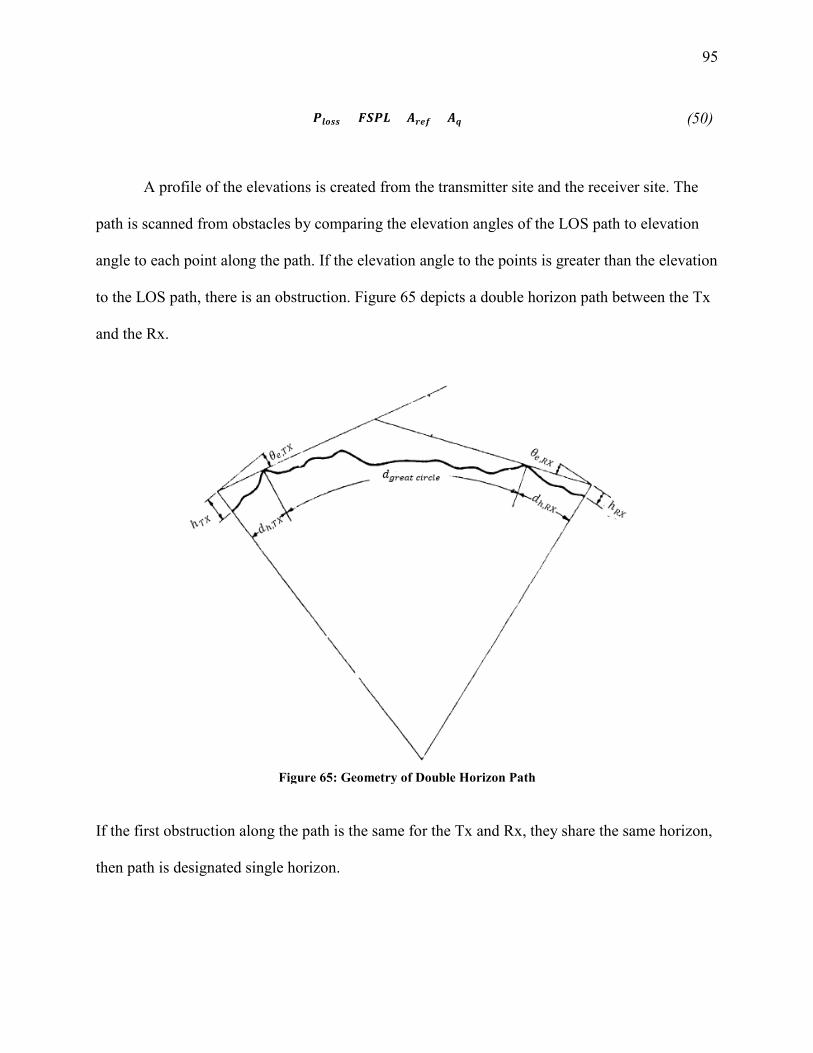
95

𝑷𝑷𝒎𝒎𝒎𝒎𝑵𝑵𝑵𝑵 = 𝑵𝑵𝑺𝑺𝑷𝑷𝑳𝑳 + 𝑨𝑨𝒍𝒍𝒃𝒃𝟐𝟐 + 𝑨𝑨𝒆𝒆 (50)

A profile of the elevations is created from the transmitter site and the receiver site. The

path is scanned from obstacles by comparing the elevation angles of the LOS path to elevation

angle to each point along the path. If the elevation angle to the points is greater than the elevation

to the LOS path, there is an obstruction. Figure 65 depicts a double horizon path between the Tx

and the Rx.

Figure 65: Geometry of Double Horizon Path

If the first obstruction along the path is the same for the Tx and Rx, they share the same horizon,

then path is designated single horizon.

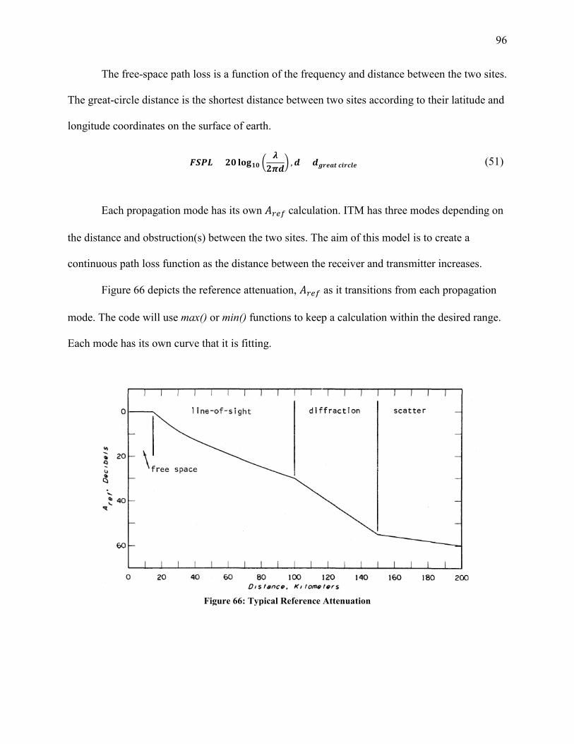
96

The free-space path loss is a function of the frequency and distance between the two sites.

The great-circle distance is the shortest distance between two sites according to their latitude and

longitude coordinates on the surface of earth.

𝑵𝑵𝑺𝑺𝑷𝑷𝑳𝑳 = 𝟐𝟐𝟏𝟏 𝐥𝐥𝐜𝐜𝐥𝐥𝟏𝟏𝟏𝟏 �𝝀𝝀

𝟐𝟐𝟐𝟐𝒃𝒃� ,𝒃𝒃 = 𝒃𝒃𝒈𝒈𝒍𝒍𝒃𝒃𝒃𝒃𝒕𝒕 𝒄𝒄𝒃𝒃𝒍𝒍𝒄𝒄𝒎𝒎𝒃𝒃 (51)

Each propagation mode has its own 𝐴𝐴𝑙𝑙𝑏𝑏𝑟𝑟 calculation. ITM has three modes depending on

the distance and obstruction(s) between the two sites. The aim of this model is to create a

continuous path loss function as the distance between the receiver and transmitter increases.

Figure 66 depicts the reference attenuation, 𝐴𝐴𝑙𝑙𝑏𝑏𝑟𝑟 as it transitions from each propagation

mode. The code will use max() or min() functions to keep a calculation within the desired range.

Each mode has its own curve that it is fitting.

Figure 66: Typical Reference Attenuation

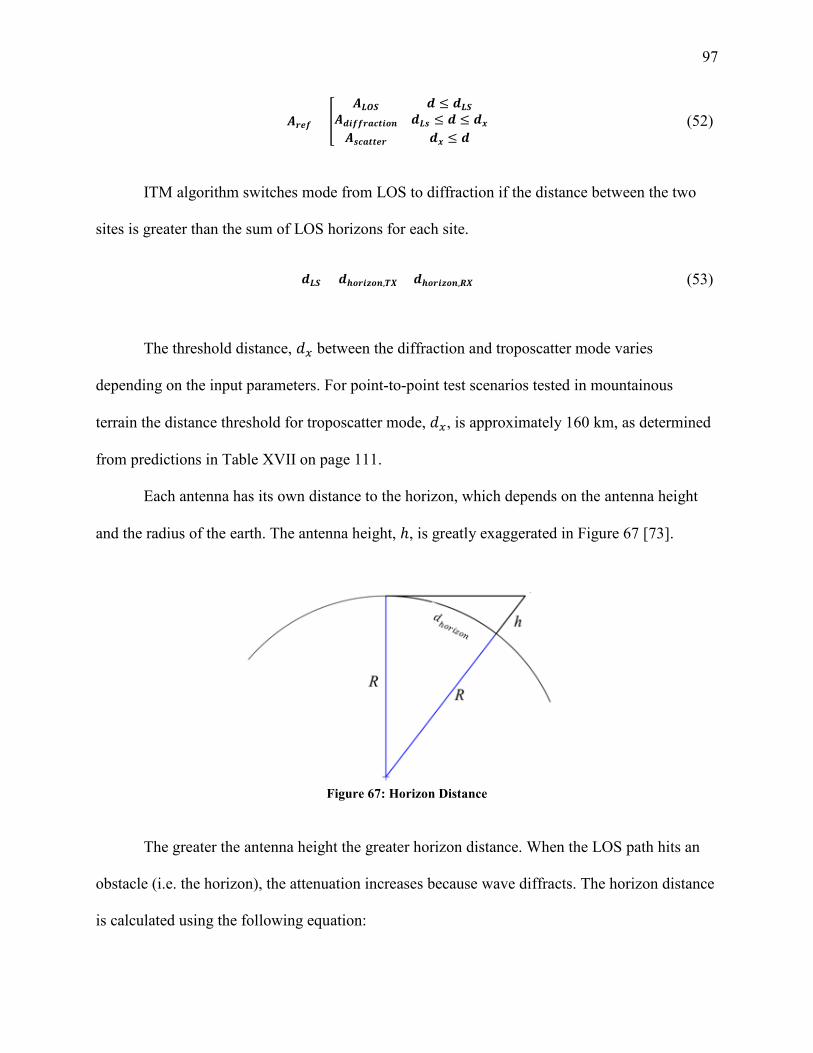
97

𝑨𝑨𝒍𝒍𝒃𝒃𝟐𝟐 = �𝑨𝑨𝑳𝑳𝑳𝑳𝑺𝑺 𝒃𝒃 ≤ 𝒃𝒃𝑳𝑳𝑺𝑺

𝑨𝑨𝒃𝒃𝒃𝒃𝟐𝟐𝟐𝟐𝒍𝒍𝒃𝒃𝒄𝒄𝒕𝒕𝒃𝒃𝒎𝒎𝒃𝒃 𝒃𝒃𝑳𝑳𝑵𝑵 ≤ 𝒃𝒃 ≤ 𝒃𝒃𝑻𝑻𝑨𝑨𝑵𝑵𝒄𝒄𝒃𝒃𝒕𝒕𝒕𝒕𝒃𝒃𝒍𝒍 𝒃𝒃𝑻𝑻 ≤ 𝒃𝒃

(52)

ITM algorithm switches mode from LOS to diffraction if the distance between the two

sites is greater than the sum of LOS horizons for each site.

𝒃𝒃𝑳𝑳𝑺𝑺 = 𝒃𝒃𝒃𝒃𝒎𝒎𝒍𝒍𝒃𝒃𝑯𝑯𝒎𝒎𝒃𝒃,𝑻𝑻𝑻𝑻 + 𝒃𝒃𝒃𝒃𝒎𝒎𝒍𝒍𝒃𝒃𝑯𝑯𝒎𝒎𝒃𝒃,𝑬𝑬𝑻𝑻 (53)

The threshold distance, 𝑑𝑑𝑇𝑇 between the diffraction and troposcatter mode varies

depending on the input parameters. For point-to-point test scenarios tested in mountainous

terrain the distance threshold for troposcatter mode, 𝑑𝑑𝑇𝑇, is approximately 160 km, as determined

from predictions in Table XVII on page 111.

Each antenna has its own distance to the horizon, which depends on the antenna height

and the radius of the earth. The antenna height, ℎ, is greatly exaggerated in Figure 67 [73].

Figure 67: Horizon Distance

The greater the antenna height the greater horizon distance. When the LOS path hits an

obstacle (i.e. the horizon), the attenuation increases because wave diffracts. The horizon distance

is calculated using the following equation:

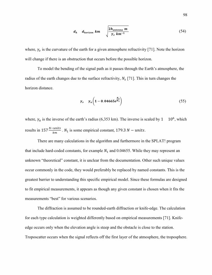
98

𝒃𝒃𝒃𝒃 = 𝒃𝒃𝒃𝒃𝒎𝒎𝒍𝒍𝒃𝒃𝑯𝑯𝒎𝒎𝒃𝒃[𝒌𝒌𝒎𝒎] = �𝟐𝟐𝒃𝒃𝒃𝒃𝒃𝒃𝒕𝒕𝒃𝒃𝒃𝒃𝒃𝒃𝒃𝒃[𝒎𝒎]𝜸𝜸𝒃𝒃[𝒌𝒌𝒎𝒎−𝟏𝟏]

(54)

where, 𝛾𝛾𝑏𝑏 is the curvature of the earth for a given atmosphere refractivity [71]. Note the horizon

will change if there is an obstruction that occurs before the possible horizon.

To model the bending of the signal path as it passes through the Earth’s atmosphere, the

radius of the earth changes due to the surface refractivity, 𝑁𝑁𝑏𝑏 [71]. This in turn changes the

horizon distance.

𝜸𝜸𝒃𝒃 = 𝜸𝜸𝒃𝒃 �𝟏𝟏 − 𝟏𝟏.𝟏𝟏𝟒𝟒𝟔𝟔𝟔𝟔𝟐𝟐𝒃𝒃𝑵𝑵𝑵𝑵𝑵𝑵𝟏𝟏� (55)

where, 𝛾𝛾𝑏𝑏 is the inverse of the earth’s radius (6,353 km). The inverse is scaled by 1 × 106, which

results in 157 𝑁𝑁−𝐽𝐽𝑏𝑏𝑙𝑙𝑟𝑟𝑏𝑏𝑘𝑘𝑚𝑚

. 𝑁𝑁1 is some empirical constant, 179.3 𝑁𝑁 − 𝑢𝑢𝑛𝑛𝑛𝑛𝑡𝑡𝐿𝐿.

There are many calculations in the algorithm and furthermore in the SPLAT! program

that include hard-coded constants, for example 𝑁𝑁1 and 0.04655. While they may represent an

unknown “theoretical” constant, it is unclear from the documentation. Other such unique values

occur commonly in the code, they would preferably be replaced by named constants. This is the

greatest barrier to understanding this specific empirical model. Since these formulas are designed

to fit empirical measurements, it appears as though any given constant is chosen when it fits the

measurements “best” for various scenarios.

The diffraction is assumed to be rounded-earth diffraction or knife-edge. The calculation

for each type calculation is weighted differently based on empirical measurements [71]. Knife-

edge occurs only when the elevation angle is steep and the obstacle is close to the station.

Troposcatter occurs when the signal reflects off the first layer of the atmosphere, the troposphere.

99

Other distance calculations include an immediate terrain distance, 𝑑𝑑𝐿𝐿, one for each

station, 𝑑𝑑𝐿𝐿,𝑇𝑇𝑇𝑇 and 𝑑𝑑𝐿𝐿,𝑅𝑅𝑇𝑇 [71]. These distances define a range of interest between the Rx and Tx

and the irregularity terrain parameter, 𝛥𝛥ℎ:

𝒃𝒃𝑳𝑳 = 𝐦𝐦𝐬𝐬𝐚𝐚(𝟏𝟏𝟐𝟐 𝒃𝒃𝒃𝒃𝒃𝒃𝒕𝒕𝒃𝒃𝒃𝒃𝒃𝒃𝒃𝒃,𝟏𝟏.𝟏𝟏 𝒃𝒃𝒃𝒃𝒎𝒎𝒍𝒍𝒃𝒃𝑯𝑯𝒎𝒎𝒃𝒃) (56)

Only the elevations along the path between these distances are used to determine the

effective antenna heights [71]. These are fitted with a least square line and the elevations on the

fitted line for the 𝑑𝑑𝐿𝐿 of each station, ℎ𝑟𝑟𝑙𝑙𝑟𝑟 = 𝑁𝑁(𝑑𝑑𝐿𝐿):

𝒃𝒃𝒃𝒃 = 𝒃𝒃𝒃𝒃𝟐𝟐𝟐𝟐𝒃𝒃𝒄𝒄𝒕𝒕𝒃𝒃𝒗𝒗𝒃𝒃 = 𝒃𝒃𝒃𝒃𝒎𝒎𝒃𝒃𝒗𝒗𝒃𝒃𝒕𝒕𝒃𝒃𝒎𝒎𝒃𝒃 + (𝒃𝒃𝒃𝒃𝒎𝒎𝒃𝒃𝒗𝒗𝒃𝒃𝒕𝒕𝒃𝒃𝒎𝒎𝒃𝒃 − 𝐦𝐦𝐬𝐬𝐚𝐚(𝒃𝒃𝒃𝒃𝒎𝒎𝒃𝒃𝒗𝒗𝒃𝒃𝒕𝒕𝒃𝒃𝒎𝒎𝒃𝒃,𝒃𝒃𝟐𝟐𝒃𝒃𝒕𝒕) (57)

Essentially, if the antenna is higher than the terrain along the path, the effective antenna

height is raised. Otherwise, it is kept the same.

The elevation heights along the path between the Rx and Tx are used to determine the

terrain irregularity parameter, 𝛥𝛥ℎ. At most twenty-five elevation heights between 𝑑𝑑𝐿𝐿,𝑅𝑅𝑇𝑇 and

𝑑𝑑𝐿𝐿,𝑇𝑇𝑇𝑇 are collected and fitted with a straight line. From this set, the inner-quartile of the

elevations are found, 𝛥𝛥ℎ(𝑑𝑑). Then formula is applied to find the irregular terrain parameter:

𝜟𝜟𝒃𝒃 =𝜟𝜟𝒃𝒃(𝒃𝒃)

�𝟏𝟏 − 𝟏𝟏.𝟖𝟖 𝒃𝒃−𝐦𝐦𝐬𝐬𝐚𝐚�𝟐𝟐𝟏𝟏,𝒃𝒃𝑫𝑫×𝟏𝟏𝟏𝟏𝟒𝟒�� (58)

where, 𝐷𝐷 = 𝑑𝑑𝑔𝑔𝑙𝑙𝑏𝑏𝑏𝑏𝑟𝑟 𝑐𝑐𝑙𝑙𝑙𝑙𝑐𝑐𝑙𝑙𝑏𝑏 − (𝑑𝑑𝐿𝐿,𝑇𝑇𝑇𝑇 + 𝑑𝑑𝐿𝐿,𝑅𝑅𝑇𝑇) and 𝑑𝑑𝐿𝐿 is the immediate terrain distance for each

antenna (see Equation 55) [71]. Lastly, the elevation angles from the Tx or Rx to the horizon is

determined:

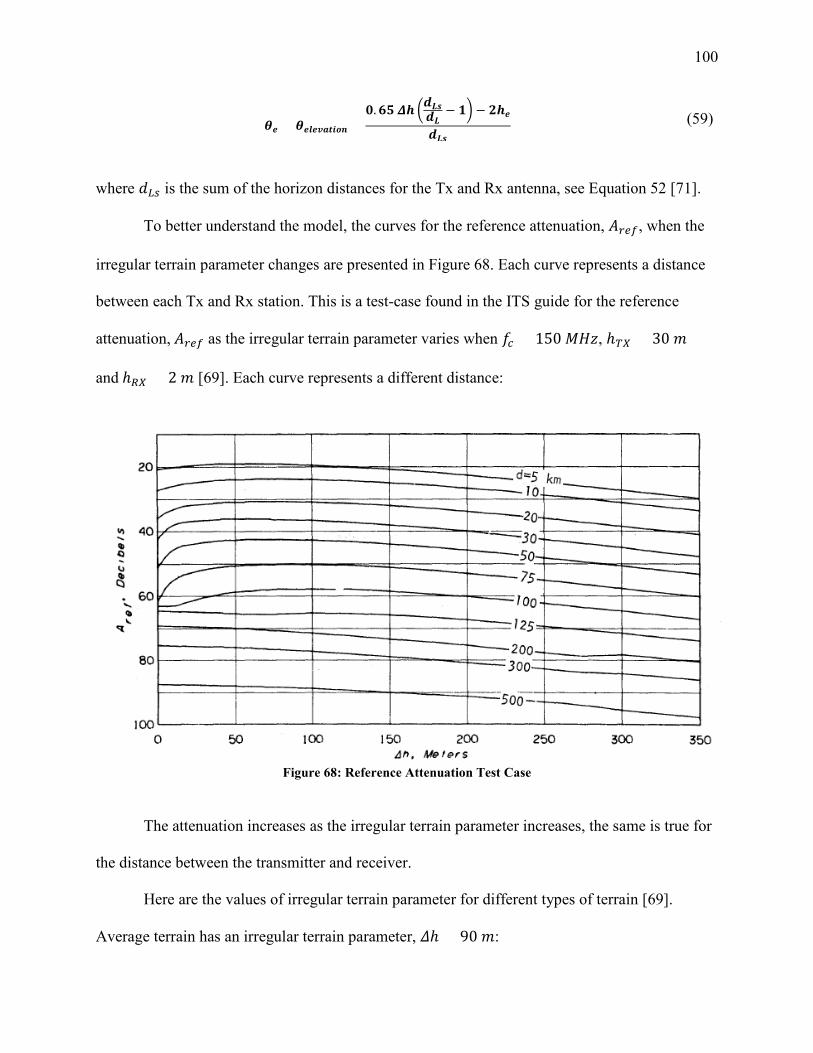
100

𝜽𝜽𝒃𝒃 = 𝜽𝜽𝒃𝒃𝒎𝒎𝒃𝒃𝒗𝒗𝒃𝒃𝒕𝒕𝒃𝒃𝒎𝒎𝒃𝒃 =𝟏𝟏.𝟔𝟔𝟐𝟐 𝜟𝜟𝒃𝒃 �𝒃𝒃𝑳𝑳𝑵𝑵𝒃𝒃𝑳𝑳

− 𝟏𝟏� − 𝟐𝟐𝒃𝒃𝒃𝒃𝒃𝒃𝑳𝑳𝑵𝑵

(59)

where 𝑑𝑑𝐿𝐿𝑏𝑏 is the sum of the horizon distances for the Tx and Rx antenna, see Equation 52 [71].

To better understand the model, the curves for the reference attenuation, 𝐴𝐴𝑙𝑙𝑏𝑏𝑟𝑟, when the

irregular terrain parameter changes are presented in Figure 68. Each curve represents a distance

between each Tx and Rx station. This is a test-case found in the ITS guide for the reference

attenuation, 𝐴𝐴𝑙𝑙𝑏𝑏𝑟𝑟 as the irregular terrain parameter varies when 𝑓𝑓𝑐𝑐 = 150 𝐼𝐼𝑀𝑀𝑀𝑀, ℎ𝑇𝑇𝑇𝑇 = 30 𝑑𝑑

and ℎ𝑅𝑅𝑇𝑇 = 2 𝑑𝑑 [69]. Each curve represents a different distance:

Figure 68: Reference Attenuation Test Case

The attenuation increases as the irregular terrain parameter increases, the same is true for

the distance between the transmitter and receiver.

Here are the values of irregular terrain parameter for different types of terrain [69].

Average terrain has an irregular terrain parameter, 𝛥𝛥ℎ = 90 𝑑𝑑:

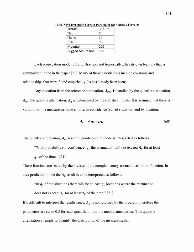
101

Table XIV: Irregular Terrain Parameter for Various Terrains Terrain 𝛥𝛥ℎ (𝑑𝑑) Flat 0 Plains 30 Hills 90 Mountain 200 Rugged Mountains 500

Each propagation mode: LOS, diffraction and troposcatter, has its own formula that is

summarized in the in the paper [71]. Many of these calculations include constants and

relationships that were found empirically (as has already been seen).

Any deviation from the reference attenuation, 𝐴𝐴𝑙𝑙𝑏𝑏𝑟𝑟 is handled by the quantile attenuation,

𝐴𝐴𝑞𝑞. The quantile attenuation, 𝐴𝐴𝑞𝑞 is determined by the statistical inputs. It is assumed that there is

variation of the measurements over time, in confidence (called situation) and by location:

𝑨𝑨𝒆𝒆 = 𝑨𝑨(𝒆𝒆𝑻𝑻,𝒆𝒆𝑺𝑺,𝒆𝒆𝑳𝑳) (60)

The quantile attenuation, 𝐴𝐴𝑞𝑞, result in point-to-point mode is interpreted as follows:

“With probability (or confidence) 𝑞𝑞𝑏𝑏 the attenuation will not exceed 𝐴𝐴𝑞𝑞 for at least

𝑞𝑞𝑇𝑇 of the time.” [71]

These fractions are scaled by the inverse of the complementary normal distribution function. In

area prediction mode the 𝐴𝐴𝑞𝑞 result is to be interpreted as follows:

“In 𝑞𝑞𝑏𝑏 of the situations there will be at least 𝑞𝑞𝐿𝐿 locations where the attenuation

does not exceed 𝐴𝐴𝑞𝑞 for at least 𝑞𝑞𝑇𝑇 of the time.” [71]

It’s difficult to interpret the results since, 𝐴𝐴𝑞𝑞 is not returned by the program, therefore the

parameters are set to 0.5 for each quantile to find the median attenuation. This quantile

attenuation attempts to quantify the distribution of the measurements.

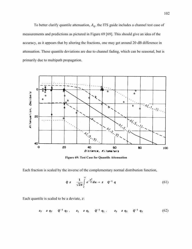
102

To better clarify quantile attenuation, 𝐴𝐴𝑞𝑞, the ITS guide includes a channel test case of

measurements and predictions as pictured in Figure 69 [69]. This should give an idea of the

accuracy, as it appears that by altering the fractions, one may get around 20 dB difference in

attenuation. These quantile deviations are due to channel fading, which can be seasonal, but is

primarily due to multipath propagation.

Figure 69: Test Case for Quantile Attenuation

Each fraction is scaled by the inverse of the complementary normal distribution function,

𝑸𝑸(𝑯𝑯) =𝟏𝟏

√𝟐𝟐𝟐𝟐� 𝒃𝒃−

𝒎𝒎𝟐𝟐𝟐𝟐 𝒃𝒃𝒎𝒎

∞

𝑯𝑯

→ 𝑯𝑯 = 𝑸𝑸−𝟏𝟏(𝒆𝒆) (61)

Each quantile is scaled to be a deviate, 𝑀𝑀:

𝑯𝑯𝑻𝑻 = 𝑯𝑯(𝒆𝒆𝑻𝑻) = 𝑸𝑸−𝟏𝟏(𝒆𝒆𝑻𝑻), 𝑯𝑯𝑳𝑳 = 𝑯𝑯(𝒆𝒆𝑳𝑳) = 𝑸𝑸−𝟏𝟏(𝒆𝒆𝑳𝑳), 𝑯𝑯𝑺𝑺 = 𝑯𝑯(𝒆𝒆𝑺𝑺) = 𝑸𝑸−𝟏𝟏(𝒆𝒆𝑺𝑺) (62)

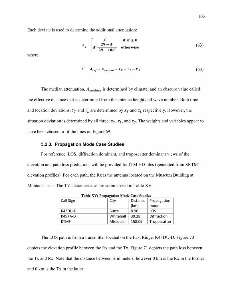
103

Each deviate is used to determine the additional attenuation:

𝑨𝑨𝒆𝒆 = �𝑨𝑨′ 𝐬𝐬𝐢𝐢 𝑨𝑨′ ≥ 𝟏𝟏

𝑨𝑨′(𝟐𝟐𝟐𝟐 − 𝑨𝑨′)

(𝟐𝟐𝟐𝟐 − 𝟏𝟏𝟏𝟏𝑨𝑨′)𝐜𝐜𝐚𝐚𝐨𝐨𝐨𝐨𝐚𝐚𝐨𝐨𝐬𝐬𝐜𝐜𝐨𝐨 (63)

where,

𝑨𝑨′ = 𝑨𝑨𝒍𝒍𝒃𝒃𝟐𝟐 − 𝑨𝑨𝒎𝒎𝒃𝒃𝒃𝒃𝒃𝒃𝒃𝒃𝒃𝒃 − 𝒀𝒀𝑻𝑻 − 𝒀𝒀𝑳𝑳 − 𝒀𝒀𝑺𝑺 (63)

The median attenuation, 𝐴𝐴𝑚𝑚𝑏𝑏𝑏𝑏𝑙𝑙𝑏𝑏𝑏𝑏 is determined by climate, and an obscure value called

the effective distance that is determined from the antenna height and wave number. Both time

and location deviations, 𝑌𝑌𝑇𝑇 and 𝑌𝑌𝐿𝐿 are determined by 𝑀𝑀𝑇𝑇 and 𝑀𝑀𝐿𝐿 respectively. However, the

situation deviation is determined by all three: 𝑀𝑀𝑇𝑇, 𝑀𝑀𝐿𝐿, and 𝑀𝑀𝑆𝑆. The weights and variables appear to

have been chosen to fit the lines on Figure 69.

5.2.3. Propagation Mode Case Studies

For reference, LOS, diffraction dominant, and troposcatter dominant views of the

elevation and path loss predictions will be provided for ITM HD files (generated from SRTM1

elevation profiles). For each path, the Rx is the antenna located on the Museum Building at

Montana Tech. The TV characteristics are summarized in Table XV.

Table XV: Propagation Mode Case Studies Call Sign City Distance

(km) Propagation mode

K43DU-D Butte 8.90 LOS K49KA-D Whitehall 39.28 Diffraction KTMF Missoula 158.09 Troposcatter

The LOS path is from a transmitter located on the East Ridge, K43DU-D. Figure 70

depicts the elevation profile between the Rx and the Tx. Figure 71 depicts the path loss between

the Tx and Rx. Note that the distance between is in meters, however 0 km is the Rx in the former

and 0 km is the Tx in the latter.

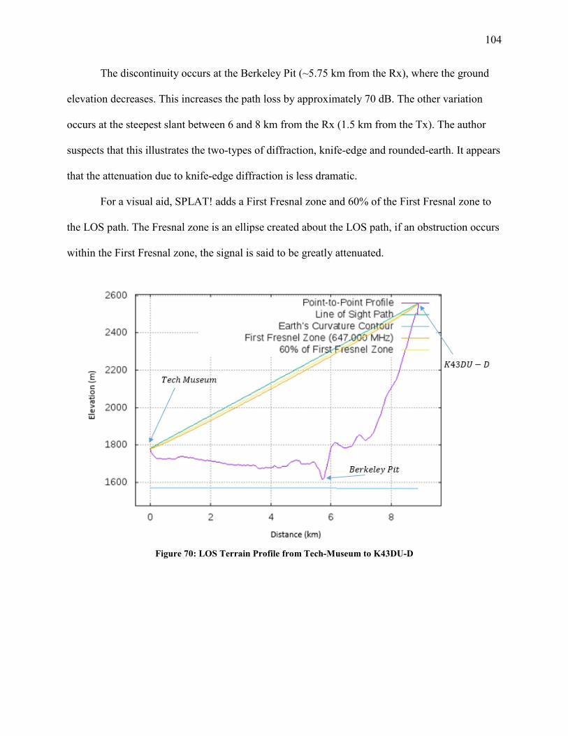
104

The discontinuity occurs at the Berkeley Pit (~5.75 km from the Rx), where the ground

elevation decreases. This increases the path loss by approximately 70 dB. The other variation

occurs at the steepest slant between 6 and 8 km from the Rx (1.5 km from the Tx). The author

suspects that this illustrates the two-types of diffraction, knife-edge and rounded-earth. It appears

that the attenuation due to knife-edge diffraction is less dramatic.

For a visual aid, SPLAT! adds a First Fresnal zone and 60% of the First Fresnal zone to

the LOS path. The Fresnal zone is an ellipse created about the LOS path, if an obstruction occurs

within the First Fresnal zone, the signal is said to be greatly attenuated.

Figure 70: LOS Terrain Profile from Tech-Museum to K43DU-D

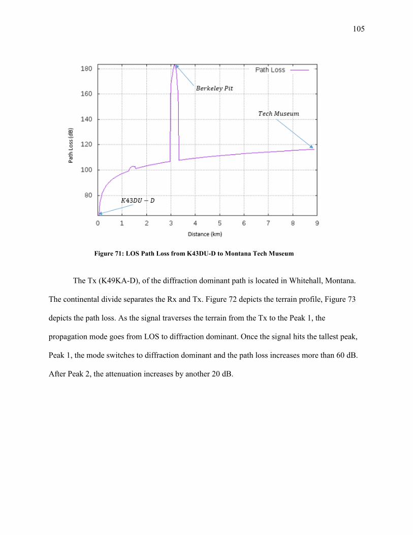
105

Figure 71: LOS Path Loss from K43DU-D to Montana Tech Museum

The Tx (K49KA-D), of the diffraction dominant path is located in Whitehall, Montana.

The continental divide separates the Rx and Tx. Figure 72 depicts the terrain profile, Figure 73

depicts the path loss. As the signal traverses the terrain from the Tx to the Peak 1, the

propagation mode goes from LOS to diffraction dominant. Once the signal hits the tallest peak,

Peak 1, the mode switches to diffraction dominant and the path loss increases more than 60 dB.

After Peak 2, the attenuation increases by another 20 dB.

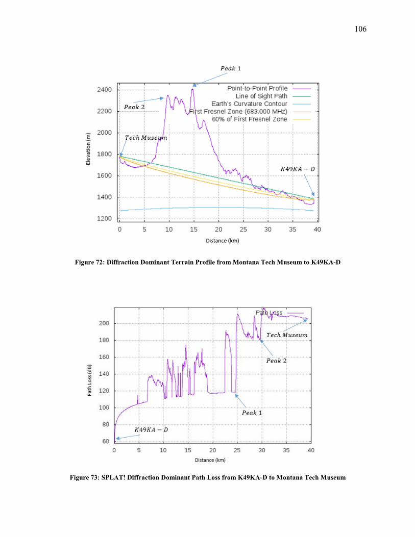
106

Figure 72: Diffraction Dominant Terrain Profile from Montana Tech Museum to K49KA-D

Figure 73: SPLAT! Diffraction Dominant Path Loss from K49KA-D to Montana Tech Museum

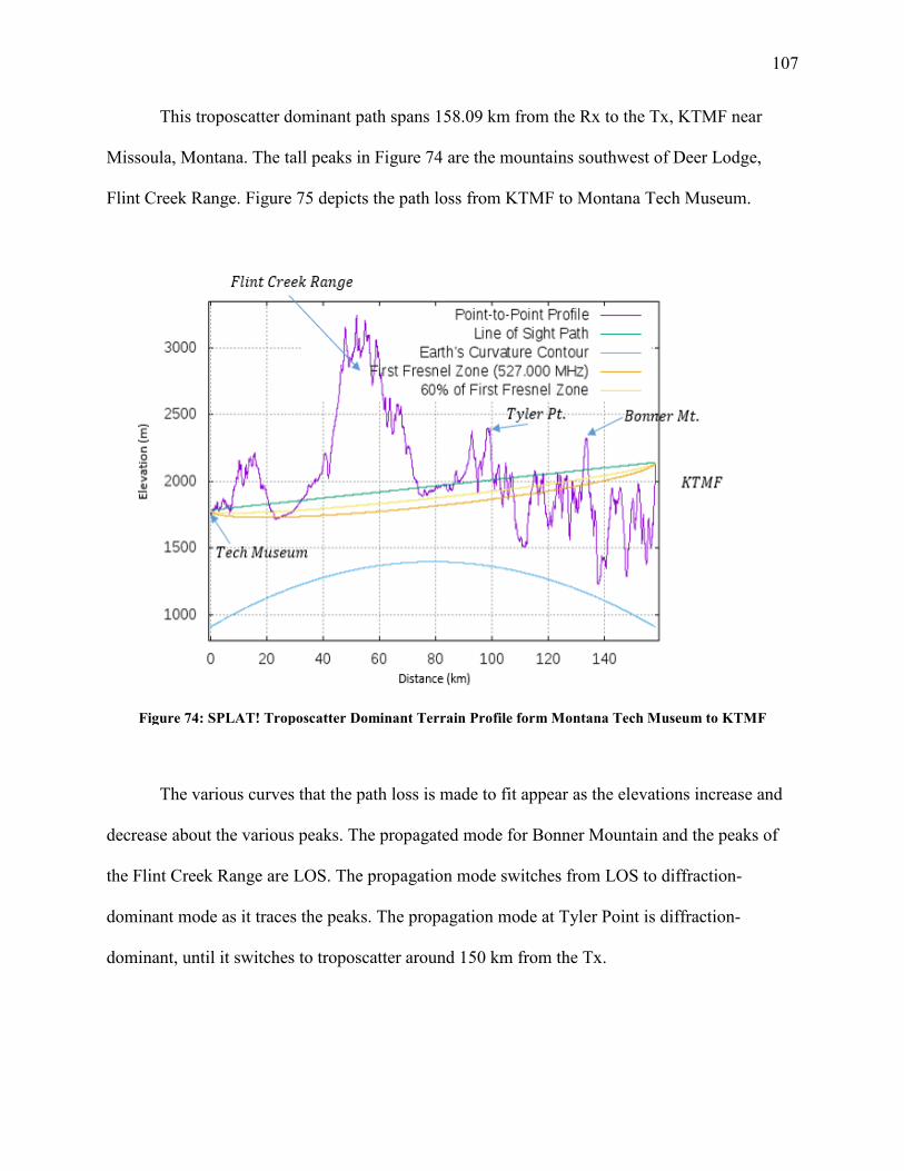
107

This troposcatter dominant path spans 158.09 km from the Rx to the Tx, KTMF near

Missoula, Montana. The tall peaks in Figure 74 are the mountains southwest of Deer Lodge,

Flint Creek Range. Figure 75 depicts the path loss from KTMF to Montana Tech Museum.

Figure 74: SPLAT! Troposcatter Dominant Terrain Profile form Montana Tech Museum to KTMF

The various curves that the path loss is made to fit appear as the elevations increase and

decrease about the various peaks. The propagated mode for Bonner Mountain and the peaks of

the Flint Creek Range are LOS. The propagation mode switches from LOS to diffraction-

dominant mode as it traces the peaks. The propagation mode at Tyler Point is diffraction-

dominant, until it switches to troposcatter around 150 km from the Tx.

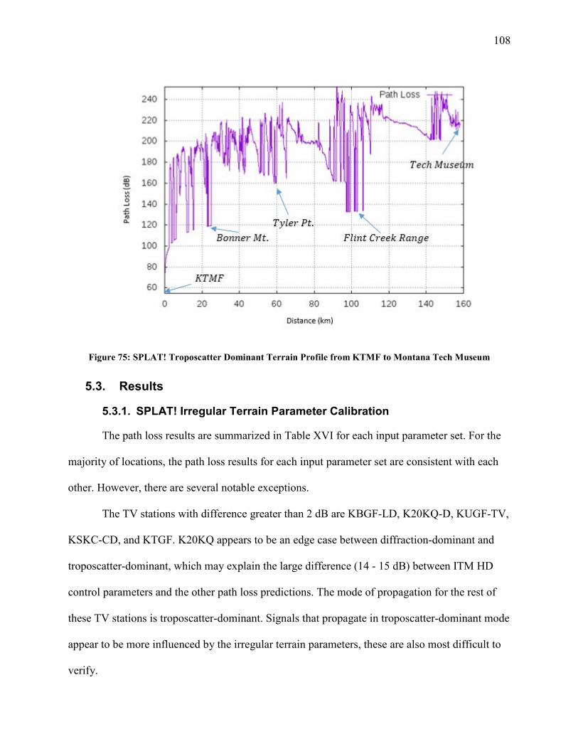
108

Figure 75: SPLAT! Troposcatter Dominant Terrain Profile from KTMF to Montana Tech Museum

5.3. Results

5.3.1. SPLAT! Irregular Terrain Parameter Calibration

The path loss results are summarized in Table XVI for each input parameter set. For the

majority of locations, the path loss results for each input parameter set are consistent with each

other. However, there are several notable exceptions.

The TV stations with difference greater than 2 dB are KBGF-LD, K20KQ-D, KUGF-TV,

KSKC-CD, and KTGF. K20KQ appears to be an edge case between diffraction-dominant and

troposcatter-dominant, which may explain the large difference (14 - 15 dB) between ITM HD

control parameters and the other path loss predictions. The mode of propagation for the rest of

these TV stations is troposcatter-dominant. Signals that propagate in troposcatter-dominant mode

appear to be more influenced by the irregular terrain parameters, these are also most difficult to

verify.

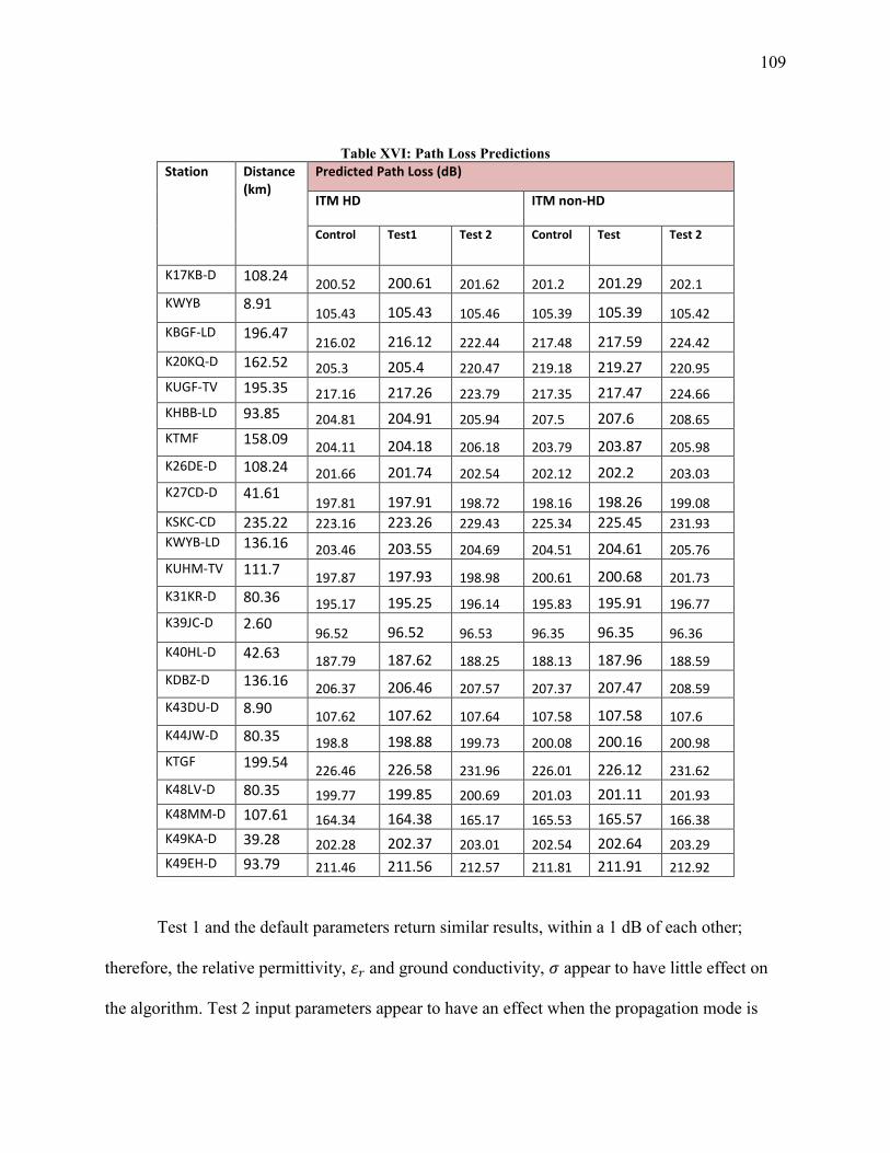
109

Table XVI: Path Loss Predictions Station Distance

(km) Predicted Path Loss (dB)

ITM HD ITM non-HD

Control Test1 Test 2 Control Test Test 2

K17KB-D 108.24 200.52 200.61 201.62 201.2 201.29 202.1 KWYB 8.91

105.43 105.43 105.46 105.39 105.39 105.42 KBGF-LD 196.47

216.02 216.12 222.44 217.48 217.59 224.42 K20KQ-D 162.52 205.3 205.4 220.47 219.18 219.27 220.95 KUGF-TV 195.35 217.16 217.26 223.79 217.35 217.47 224.66 KHBB-LD 93.85 204.81 204.91 205.94 207.5 207.6 208.65 KTMF 158.09 204.11 204.18 206.18 203.79 203.87 205.98 K26DE-D 108.24 201.66 201.74 202.54 202.12 202.2 203.03 K27CD-D 41.61

197.81 197.91 198.72 198.16 198.26 199.08 KSKC-CD 235.22 223.16 223.26 229.43 225.34 225.45 231.93 KWYB-LD 136.16 203.46 203.55 204.69 204.51 204.61 205.76 KUHM-TV 111.7 197.87 197.93 198.98 200.61 200.68 201.73 K31KR-D 80.36 195.17 195.25 196.14 195.83 195.91 196.77 K39JC-D 2.60

96.52 96.52 96.53 96.35 96.35 96.36 K40HL-D 42.63 187.79 187.62 188.25 188.13 187.96 188.59 KDBZ-D 136.16 206.37 206.46 207.57 207.37 207.47 208.59 K43DU-D 8.90 107.62 107.62 107.64 107.58 107.58 107.6 K44JW-D 80.35 198.8 198.88 199.73 200.08 200.16 200.98 KTGF 199.54 226.46 226.58 231.96 226.01 226.12 231.62 K48LV-D 80.35 199.77 199.85 200.69 201.03 201.11 201.93 K48MM-D 107.61 164.34 164.38 165.17 165.53 165.57 166.38 K49KA-D 39.28 202.28 202.37 203.01 202.54 202.64 203.29 K49EH-D 93.79 211.46 211.56 212.57 211.81 211.91 212.92

Test 1 and the default parameters return similar results, within a 1 dB of each other;

therefore, the relative permittivity, 𝜀𝜀𝑟𝑟 and ground conductivity, 𝜎𝜎 appear to have little effect on

the algorithm. Test 2 input parameters appear to have an effect when the propagation mode is

110

troposcatter-dominant; other LOS and diffraction-dominant path loss results are within 2 dB of

the other predictions.

The propagation mode for each station and test parameter is summarized in Table XVII.

The difference in path loss between each mode is instructive, since it gives a general sense of

propagation in a mountainous terrain. For the default parameters and HD, i.e. SRTM1 elevation

files, the troposcatter dominant propagation have path loss predictions that range from 150 to

235 dB. The diffraction dominant range is from 164 dB to 204 dB. The LOS path loss

predictions vary from 96 to 107 dB.

The discontinuity between LOS and diffraction mode is most drastic. Once the mode of

propagation is no longer LOS, the path loss increases by at least 50 dB, which means that the

signal is 100,000 times smaller. The difference can be as much as 80 dB, which is 100 million

times smaller. It can even be 100 dB, which is 10 billion times smaller. These trends may be seen

in the reference figures (Figs. 70 to 75) where the path loss across the distance from the TV

station to the Montana Tech Museum is shown.

For both sets of input parameters, Control and Test, there is little difference between ITM

HD and ITM non-HD. K20KQ is an exception for reasons discussed previously. In order to save

computation time, it appears as though it is acceptable to substitute ITM non-HD for ITM HD.

The path loss prediction for the population grids implemented ITM non-HD elevation files:

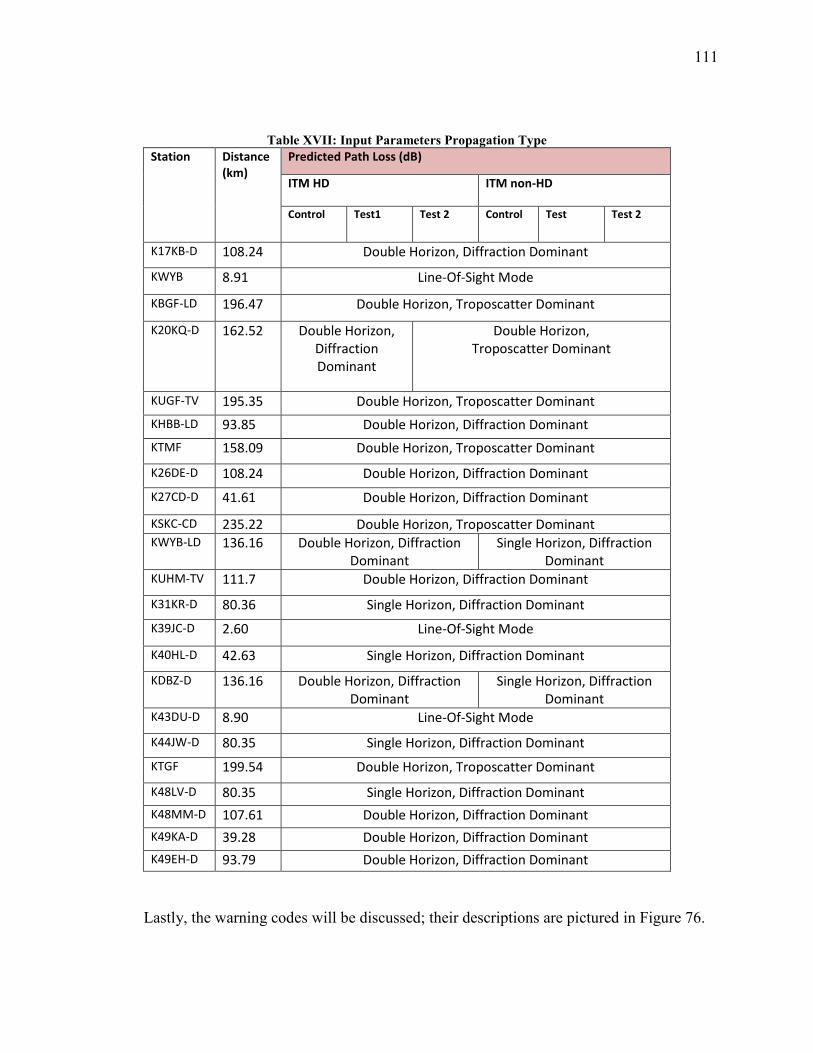
111

Table XVII: Input Parameters Propagation Type Station Distance

(km) Predicted Path Loss (dB)

ITM HD ITM non-HD

Control Test1 Test 2 Control Test Test 2

K17KB-D 108.24 Double Horizon, Diffraction Dominant

KWYB 8.91 Line-Of-Sight Mode

KBGF-LD 196.47 Double Horizon, Troposcatter Dominant

K20KQ-D 162.52 Double Horizon, Diffraction Dominant

Double Horizon, Troposcatter Dominant

KUGF-TV 195.35 Double Horizon, Troposcatter Dominant

KHBB-LD 93.85 Double Horizon, Diffraction Dominant

KTMF 158.09 Double Horizon, Troposcatter Dominant

K26DE-D 108.24 Double Horizon, Diffraction Dominant

K27CD-D 41.61 Double Horizon, Diffraction Dominant

KSKC-CD 235.22 Double Horizon, Troposcatter Dominant KWYB-LD 136.16 Double Horizon, Diffraction

Dominant Single Horizon, Diffraction

Dominant KUHM-TV 111.7 Double Horizon, Diffraction Dominant

K31KR-D 80.36 Single Horizon, Diffraction Dominant

K39JC-D 2.60 Line-Of-Sight Mode

K40HL-D 42.63 Single Horizon, Diffraction Dominant

KDBZ-D 136.16 Double Horizon, Diffraction Dominant

Single Horizon, Diffraction Dominant

K43DU-D 8.90 Line-Of-Sight Mode

K44JW-D 80.35 Single Horizon, Diffraction Dominant

KTGF 199.54 Double Horizon, Troposcatter Dominant

K48LV-D 80.35 Single Horizon, Diffraction Dominant

K48MM-D 107.61 Double Horizon, Diffraction Dominant

K49KA-D 39.28 Double Horizon, Diffraction Dominant

K49EH-D 93.79 Double Horizon, Diffraction Dominant

Lastly, the warning codes will be discussed; their descriptions are pictured in Figure 76.

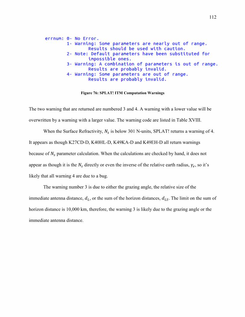
112

Figure 76: SPLAT! ITM Computation Warnings

The two warning that are returned are numbered 3 and 4. A warning with a lower value will be

overwritten by a warning with a larger value. The warning code are listed in Table XVIII.

When the Surface Refractivity, 𝑁𝑁𝑏𝑏 is below 301 N-units, SPLAT! returns a warning of 4.

It appears as though K27CD-D, K40HL-D, K49KA-D and K49EH-D all return warnings

because of 𝑁𝑁𝑏𝑏 parameter calculation. When the calculations are checked by hand, it does not

appear as though it is the 𝑁𝑁𝑏𝑏 directly or even the inverse of the relative earth radius, 𝛾𝛾𝑏𝑏, so it’s

likely that all warning 4 are due to a bug.

The warning number 3 is due to either the grazing angle, the relative size of the

immediate antenna distance, 𝑑𝑑𝐿𝐿, or the sum of the horizon distances, 𝑑𝑑𝐿𝐿𝑆𝑆. The limit on the sum of

horizon distance is 10,000 km, therefore, the warning 3 is likely due to the grazing angle or the

immediate antenna distance.

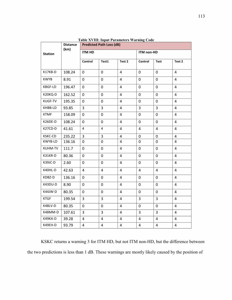
113

Table XVIII: Input Parameters Warning Code Station

Distance (km)

Predicted Path Loss (dB)

ITM HD

ITM non-HD

Control Test1

Test 2 Control Test Test 2

K17KB-D 108.24 0 0 4 0 0 4

KWYB 8.91 0 0 4 0 0 4

KBGF-LD 196.47 0 0 4 0 0 4

K20KQ-D 162.52 0 0 4 0 0 4

KUGF-TV 195.35 0 0 4 0 0 4

KHBB-LD 93.85 3 3 4 3 3 4

KTMF 158.09 0 0 4 0 0 4

K26DE-D 108.24 0 0 4 0 0 4

K27CD-D 41.61 4 4 4 4 4 4

KSKC-CD 235.22 3 3 4 0 0 4 KWYB-LD 136.16 0 0 4 0 0 4

KUHM-TV 111.7 0 0 4 0 0 4

K31KR-D 80.36 0 0 4 0 0 4

K39JC-D 2.60 0 0 4 0 0 4

K40HL-D 42.63 4 4 4 4 4 4

KDBZ-D 136.16 0 0 4 0 0 4

K43DU-D 8.90 0 0 4 0 0 4

K44JW-D 80.35 0 0 4 0 0 4

KTGF 199.54 3 3 4 3 3 4

K48LV-D 80.35 0 0 4 0 0 4

K48MM-D 107.61 3 3 4 3 3 4

K49KA-D 39.28 4 4 4 4 4 4

K49EH-D 93.79 4 4 4 4 4 4

KSKC returns a warning 3 for ITM HD, but not ITM non-HD, but the difference between

the two predictions is less than 1 dB. These warnings are mostly likely caused by the position of

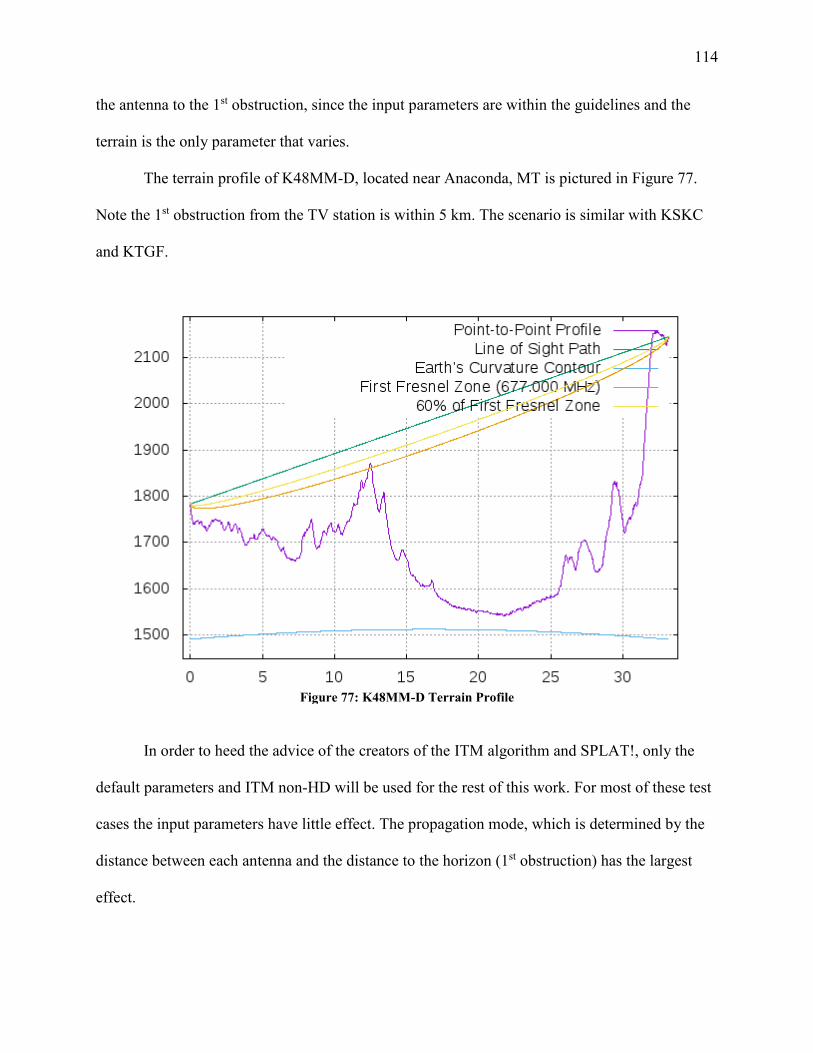
114

the antenna to the 1st obstruction, since the input parameters are within the guidelines and the

terrain is the only parameter that varies.

The terrain profile of K48MM-D, located near Anaconda, MT is pictured in Figure 77.

Note the 1st obstruction from the TV station is within 5 km. The scenario is similar with KSKC

and KTGF.

Figure 77: K48MM-D Terrain Profile

In order to heed the advice of the creators of the ITM algorithm and SPLAT!, only the

default parameters and ITM non-HD will be used for the rest of this work. For most of these test

cases the input parameters have little effect. The propagation mode, which is determined by the

distance between each antenna and the distance to the horizon (1st obstruction) has the largest

effect.

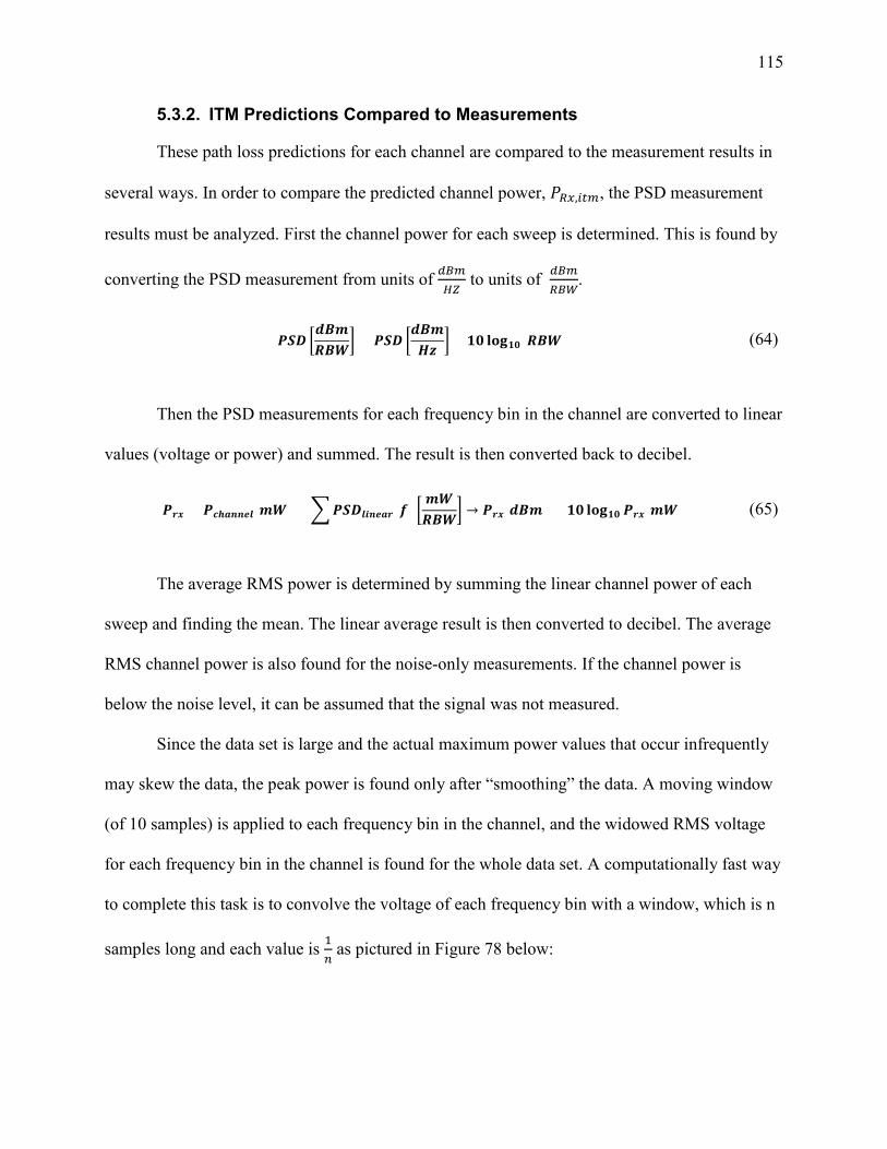
115

5.3.2. ITM Predictions Compared to Measurements

These path loss predictions for each channel are compared to the measurement results in

several ways. In order to compare the predicted channel power, 𝑃𝑃𝑅𝑅𝑇𝑇,𝑙𝑙𝑟𝑟𝑚𝑚, the PSD measurement

results must be analyzed. First the channel power for each sweep is determined. This is found by

converting the PSD measurement from units of 𝑏𝑏𝑑𝑑𝑚𝑚𝐻𝐻𝐻𝐻

to units of 𝑏𝑏𝑑𝑑𝑚𝑚𝑅𝑅𝑑𝑑𝑚𝑚

.

𝑷𝑷𝑺𝑺𝑫𝑫 �𝒃𝒃𝒅𝒅𝒎𝒎𝑬𝑬𝒅𝒅𝒅𝒅

� = 𝑷𝑷𝑺𝑺𝑫𝑫 �𝒃𝒃𝒅𝒅𝒎𝒎𝑯𝑯𝑯𝑯

� + 𝟏𝟏𝟏𝟏 𝐥𝐥𝐜𝐜𝐥𝐥𝟏𝟏𝟏𝟏(𝑬𝑬𝒅𝒅𝒅𝒅) (64)

Then the PSD measurements for each frequency bin in the channel are converted to linear

values (voltage or power) and summed. The result is then converted back to decibel.

𝑷𝑷𝒍𝒍𝑻𝑻 = 𝑷𝑷𝒄𝒄𝒃𝒃𝒃𝒃𝒃𝒃𝒃𝒃𝒃𝒃𝒎𝒎[𝒎𝒎𝒅𝒅] = �𝑷𝑷𝑺𝑺𝑫𝑫𝒎𝒎𝒃𝒃𝒃𝒃𝒃𝒃𝒃𝒃𝒍𝒍(𝟐𝟐) �𝒎𝒎𝒅𝒅𝑬𝑬𝒅𝒅𝒅𝒅

� → 𝑷𝑷𝒍𝒍𝑻𝑻[𝒃𝒃𝒅𝒅𝒎𝒎] = 𝟏𝟏𝟏𝟏 𝐥𝐥𝐜𝐜𝐥𝐥𝟏𝟏𝟏𝟏 𝑷𝑷𝒍𝒍𝑻𝑻[𝒎𝒎𝒅𝒅] (65)

The average RMS power is determined by summing the linear channel power of each

sweep and finding the mean. The linear average result is then converted to decibel. The average

RMS channel power is also found for the noise-only measurements. If the channel power is

below the noise level, it can be assumed that the signal was not measured.

Since the data set is large and the actual maximum power values that occur infrequently

may skew the data, the peak power is found only after “smoothing” the data. A moving window

(of 10 samples) is applied to each frequency bin in the channel, and the widowed RMS voltage

for each frequency bin in the channel is found for the whole data set. A computationally fast way

to complete this task is to convolve the voltage of each frequency bin with a window, which is n

samples long and each value is 1𝑏𝑏 as pictured in Figure 78 below:

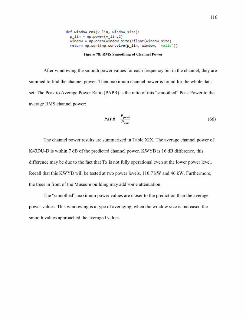
116

Figure 78: RMS Smoothing of Channel Power

After windowing the smooth power values for each frequency bin in the channel, they are

summed to find the channel power. Then maximum channel power is found for the whole data

set. The Peak to Average Power Ratio (PAPR) is the ratio of this “smoothed” Peak Power to the

average RMS channel power:

𝑷𝑷𝑨𝑨𝑷𝑷𝑬𝑬 =𝑷𝑷𝒑𝒑𝒃𝒃𝒃𝒃𝒌𝒌𝑷𝑷𝒍𝒍𝒎𝒎𝑵𝑵

(66)

The channel power results are summarized in Table XIX. The average channel power of

K43DU-D is within 7 dB of the predicted channel power. KWYB is 16 dB difference, this

difference may be due to the fact that Tx is not fully operational even at the lower power level.

Recall that this KWYB will be tested at two power levels, 110.7 kW and 46 kW. Furthermore,

the trees in front of the Museum building may add some attenuation.

The “smoothed” maximum power values are closer to the prediction than the average

power values. This windowing is a type of averaging, when the window size is increased the

smooth values approached the averaged values.

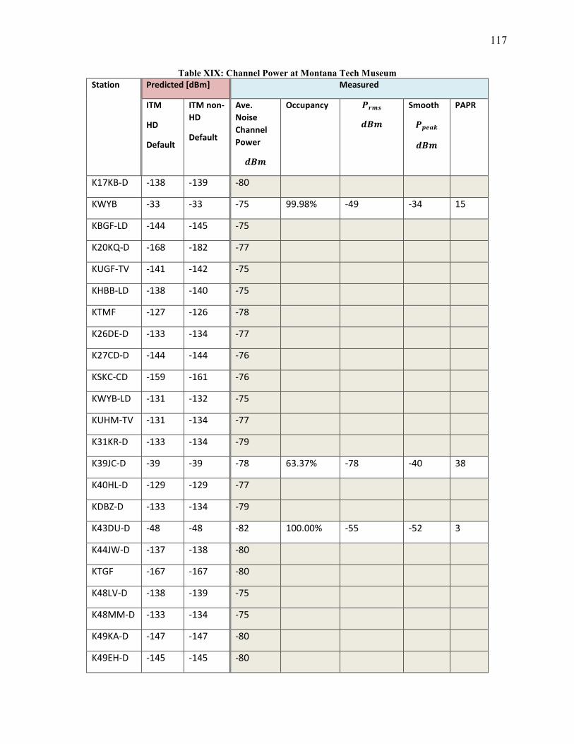
117

Table XIX: Channel Power at Montana Tech Museum Station Predicted [dBm] Measured

ITM

HD

Default

ITM non-HD

Default

Ave. Noise Channel Power

[𝒃𝒃𝒅𝒅𝒎𝒎]

Occupancy 𝑷𝑷𝒍𝒍𝒎𝒎𝑵𝑵

[𝒃𝒃𝒅𝒅𝒎𝒎]

Smooth

𝑷𝑷𝒑𝒑𝒃𝒃𝒃𝒃𝒌𝒌

[𝒃𝒃𝒅𝒅𝒎𝒎]

PAPR

K17KB-D -138 -139 -80

KWYB -33 -33 -75 99.98% -49 -34 15

KBGF-LD -144 -145 -75

K20KQ-D -168 -182 -77

KUGF-TV -141 -142 -75

KHBB-LD -138 -140 -75

KTMF -127 -126 -78

K26DE-D -133 -134 -77

K27CD-D -144 -144 -76

KSKC-CD -159 -161 -76

KWYB-LD -131 -132 -75

KUHM-TV -131 -134 -77

K31KR-D -133 -134 -79

K39JC-D -39 -39 -78 63.37% -78 -40 38

K40HL-D -129 -129 -77

KDBZ-D -133 -134 -79

K43DU-D -48 -48 -82 100.00% -55 -52 3

K44JW-D -137 -138 -80

KTGF -167 -167 -80

K48LV-D -138 -139 -75

K48MM-D -133 -134 -75

K49KA-D -147 -147 -80

K49EH-D -145 -145 -80

118

Only signals that are LOS are able to be received by antenna at the Montana Tech

Museum building. According to SPLAT!, the stations as close as Whitehall (around ~40 km

distance from Butte), K40HL-D and K49KA, and Anaconda, K48MM-D are essentially blocked

by the mountainous terrain. The attenuation increases dramatically when the signal propagates as

diffraction dominant. Any signal that propagates in troposcatter-dominant mode would be

difficult to verify, since it would require sensitivity at the receiver well below the noise floor.

It should be noted that the harmonic signal at 625 MHz is located in K39JC-D channel. It

is likely that K39JC-D transmitter is licensed but not operational or operates only occasionally.

These predicted channel characteristics are positive from an interference point-of-view.

The transmitters that are co-channel and separated by any mountainous terrain are less likely to

interfere with each other. However, from a propagation point of view, a cellular network in

mountainous terrain would require a higher number of base stations than a cellular network in

flat terrain.

5.3.3. Interference Simulations

The path loss predictions were used to predict co-channel and adjacent channel

interference. Montana Tech was granted an experimental license to transmit from 510 to 550

MHZ at ERP 20 W as station, WK9XUC. The SPLAT! ITM non-HD with default parameters

was used to predict path loss for each city grid from WK9XUC and from any TV station nearby

that transmits in the 500 MHz band. The path loss predictions were used to predict the receive

power of the TV station (desired signal) and the receive power of the WK9XUC (interference

signal).

119

Once these figures are calculated, the EVM for each location is determined. A baseline

EVM was determined for the TV station and the EIN of each Rx site on the grid. The baseline

error is due only to noise. Assuming that a TV receiver system is designed to handle a maximum

EVM of 5%, then any location on the grid where the noise error causes the EVM to exceed 5% is

considered to be in a poor receiver location. As a result, any additional interference from

WKXUC is inconsequential.

Only TV stations that operate from 470 to 560 MHz and are expected to be received at

any grid location will be included in this analysis. There are two TV channels that fit these

criteria, KWYB in Butte and K27CD-D in Boulder.

Contours are made with Matplotlib functions, griddata() from the mlab module and

controurf() [74]. The python script may be seen in Figure 79. First the Rx coordinates and the

EVM are mapped to a grid with griddata(). The interpolation of the EVM between Rx points is

called natural neighbor, based on the Delaunay triangulation [75]. This method creates triangles

between the longitude and latitude points, loni and lati, then places weights on the gridded EVM.

Note to operate the features of the Matplotlib toolkit, Natgrid must be installed [76].

contourf() fills in the contours for each contour level based on the number of levels as

defined by the user. Here the color bar has an upper limit of 5% and lower limit of 0%. Anything

above 5% will have same color, anything below 0% will be left blank, since only the upper limit

‘max’ end is extended.

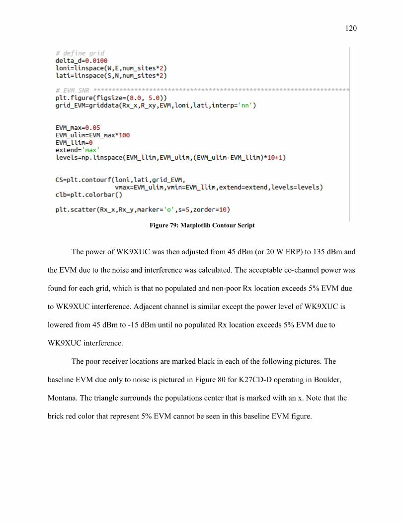
120

Figure 79: Matplotlib Contour Script

The power of WK9XUC was then adjusted from 45 dBm (or 20 W ERP) to 135 dBm and

the EVM due to the noise and interference was calculated. The acceptable co-channel power was

found for each grid, which is that no populated and non-poor Rx location exceeds 5% EVM due

to WK9XUC interference. Adjacent channel is similar except the power level of WK9XUC is

lowered from 45 dBm to -15 dBm until no populated Rx location exceeds 5% EVM due to

WK9XUC interference.

The poor receiver locations are marked black in each of the following pictures. The

baseline EVM due only to noise is pictured in Figure 80 for K27CD-D operating in Boulder,

Montana. The triangle surrounds the populations center that is marked with an x. Note that the

brick red color that represent 5% EVM cannot be seen in this baseline EVM figure.

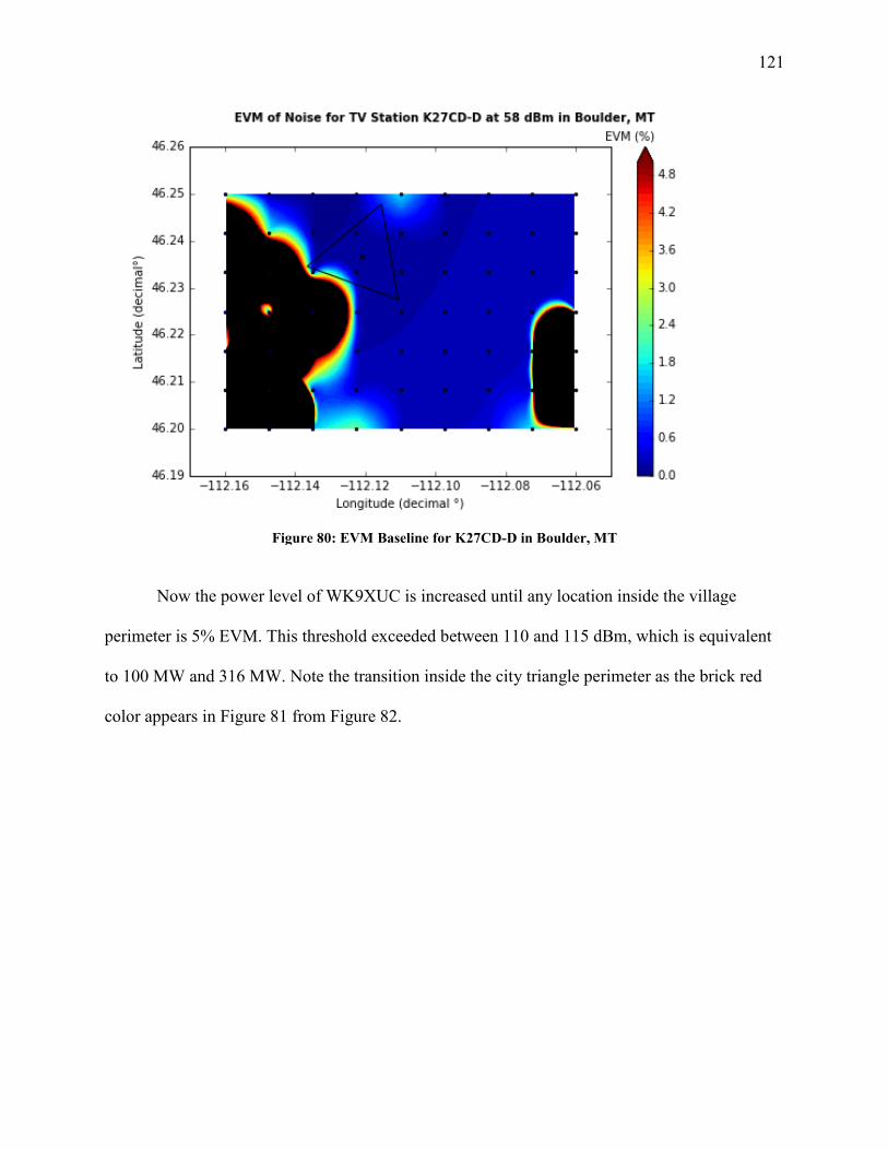
121

Figure 80: EVM Baseline for K27CD-D in Boulder, MT

Now the power level of WK9XUC is increased until any location inside the village

perimeter is 5% EVM. This threshold exceeded between 110 and 115 dBm, which is equivalent

to 100 MW and 316 MW. Note the transition inside the city triangle perimeter as the brick red

color appears in Figure 81 from Figure 82.

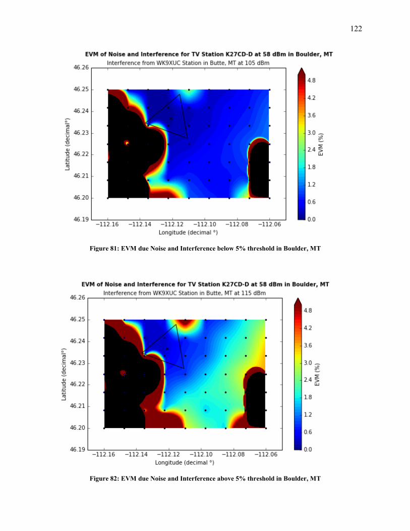
122

Figure 81: EVM due Noise and Interference below 5% threshold in Boulder, MT

Figure 82: EVM due Noise and Interference above 5% threshold in Boulder, MT

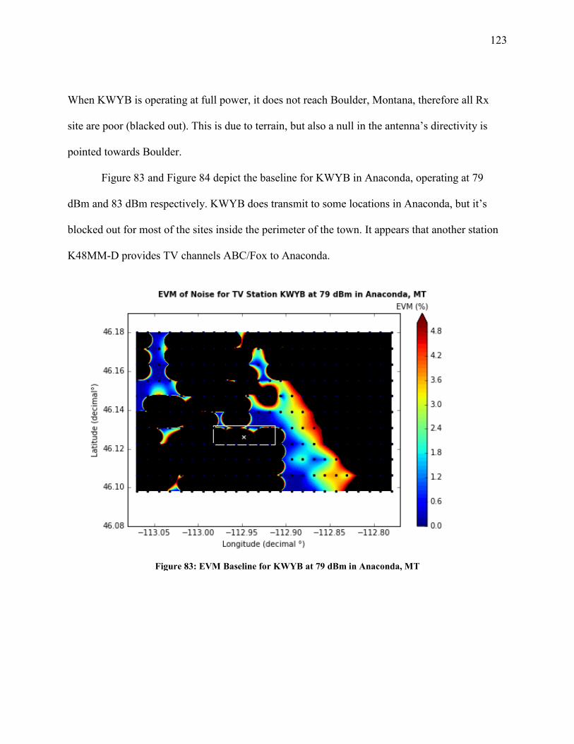
123

When KWYB is operating at full power, it does not reach Boulder, Montana, therefore all Rx

site are poor (blacked out). This is due to terrain, but also a null in the antenna’s directivity is

pointed towards Boulder.

Figure 83 and Figure 84 depict the baseline for KWYB in Anaconda, operating at 79

dBm and 83 dBm respectively. KWYB does transmit to some locations in Anaconda, but it’s

blocked out for most of the sites inside the perimeter of the town. It appears that another station

K48MM-D provides TV channels ABC/Fox to Anaconda.

Figure 83: EVM Baseline for KWYB at 79 dBm in Anaconda, MT

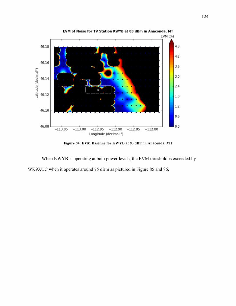
124

Figure 84: EVM Baseline for KWYB at 83 dBm in Anaconda, MT

When KWYB is operating at both power levels, the EVM threshold is exceeded by

WK9XUC when it operates around 75 dBm as pictured in Figure 85 and 86.

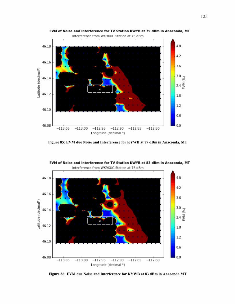
125

Figure 85: EVM due Noise and Interference for KYWB at 79 dBm in Anaconda, MT

Figure 86: EVM due Noise and Interference for KYWB at 83 dBm in Anaconda,MT

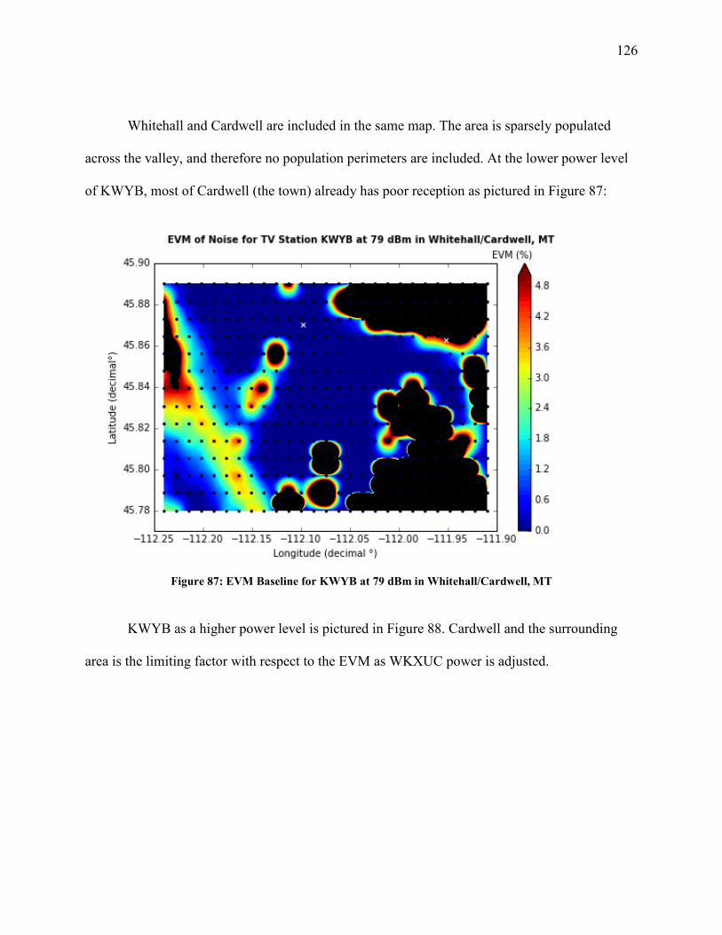
126

Whitehall and Cardwell are included in the same map. The area is sparsely populated

across the valley, and therefore no population perimeters are included. At the lower power level

of KWYB, most of Cardwell (the town) already has poor reception as pictured in Figure 87:

Figure 87: EVM Baseline for KWYB at 79 dBm in Whitehall/Cardwell, MT

KWYB as a higher power level is pictured in Figure 88. Cardwell and the surrounding

area is the limiting factor with respect to the EVM as WKXUC power is adjusted.

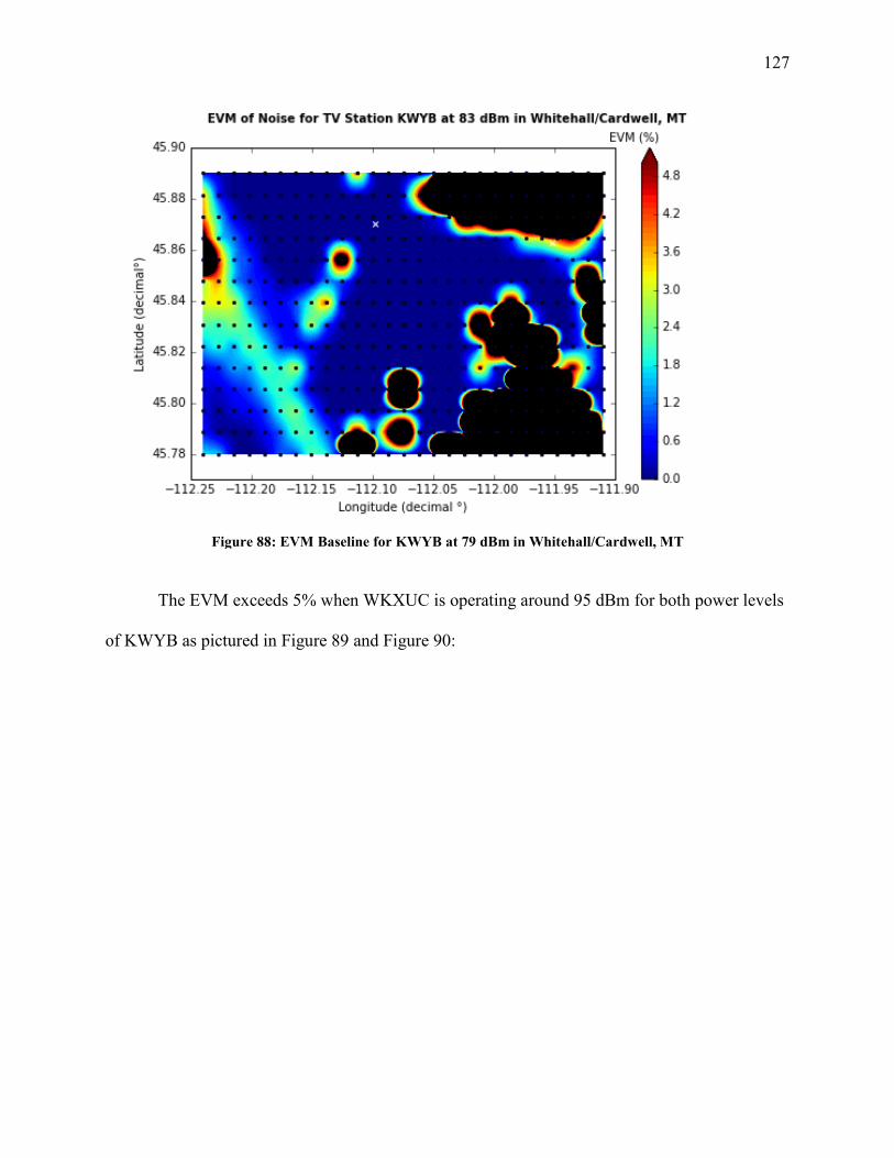
127

Figure 88: EVM Baseline for KWYB at 79 dBm in Whitehall/Cardwell, MT

The EVM exceeds 5% when WKXUC is operating around 95 dBm for both power levels

of KWYB as pictured in Figure 89 and Figure 90:

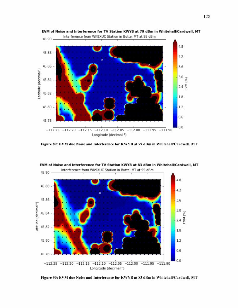
128

Figure 89: EVM due Noise and Interference for KWYB at 79 dBm in Whitehall/Cardwell, MT

Figure 90: EVM due Noise and Interference for KWYB at 83 dBm in Whitehall/Cardwell, MT

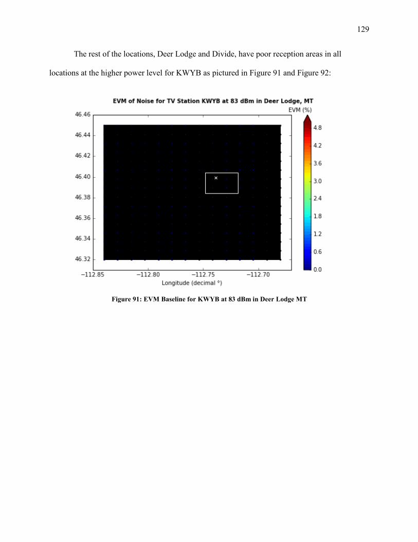
129

The rest of the locations, Deer Lodge and Divide, have poor reception areas in all

locations at the higher power level for KWYB as pictured in Figure 91 and Figure 92:

Figure 91: EVM Baseline for KWYB at 83 dBm in Deer Lodge MT

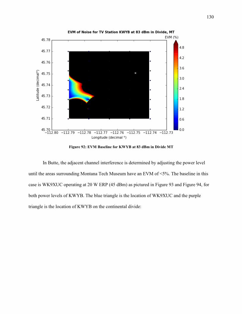
130

Figure 92: EVM Baseline for KWYB at 83 dBm in Divide MT

In Butte, the adjacent channel interference is determined by adjusting the power level

until the areas surrounding Montana Tech Museum have an EVM of <5%. The baseline in this

case is WK9XUC operating at 20 W ERP (45 dBm) as pictured in Figure 93 and Figure 94, for

both power levels of KWYB. The blue triangle is the location of WK9XUC and the purple

triangle is the location of KWYB on the continental divide:

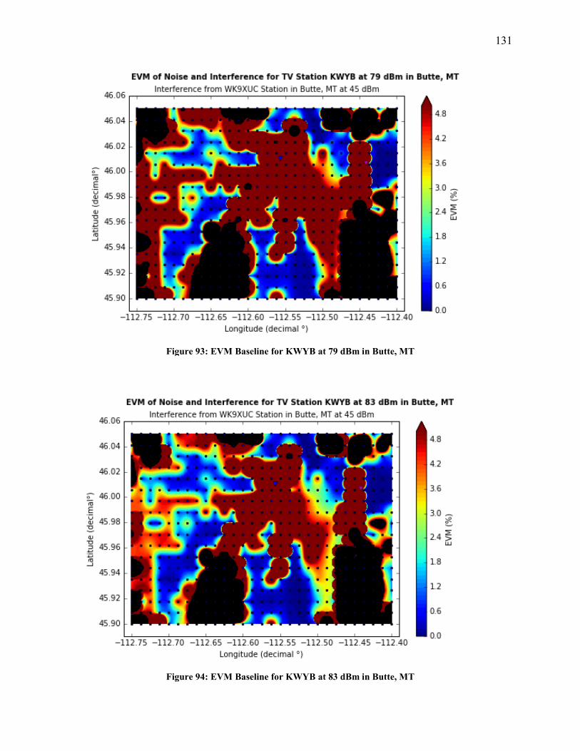
131

Figure 93: EVM Baseline for KWYB at 79 dBm in Butte, MT

Figure 94: EVM Baseline for KWYB at 83 dBm in Butte, MT

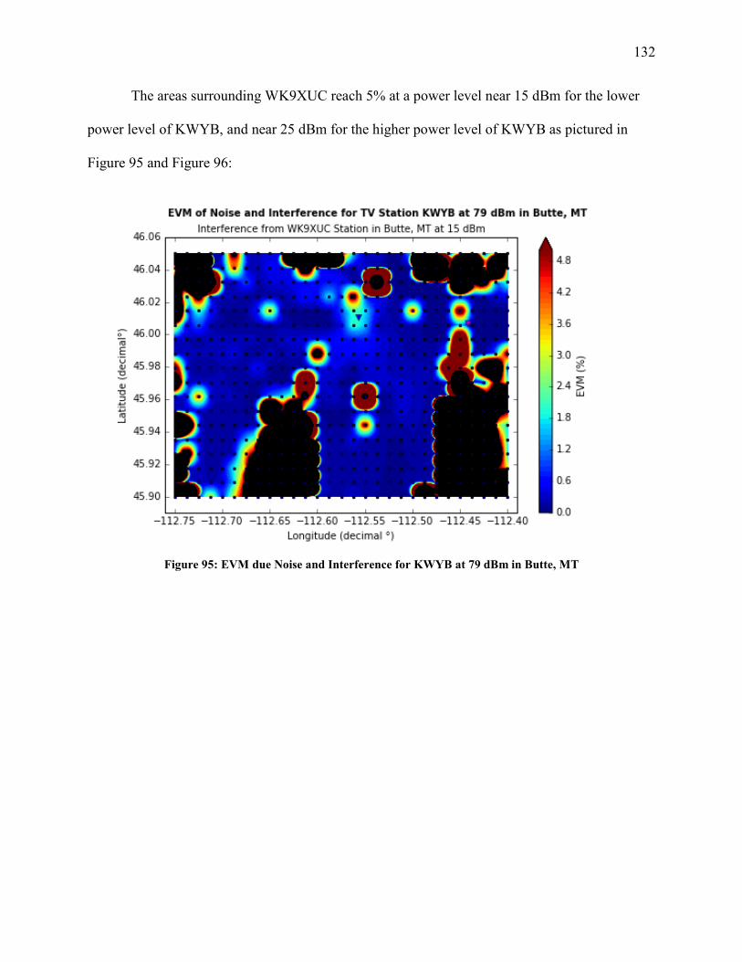
132

The areas surrounding WK9XUC reach 5% at a power level near 15 dBm for the lower

power level of KWYB, and near 25 dBm for the higher power level of KWYB as pictured in

Figure 95 and Figure 96:

Figure 95: EVM due Noise and Interference for KWYB at 79 dBm in Butte, MT

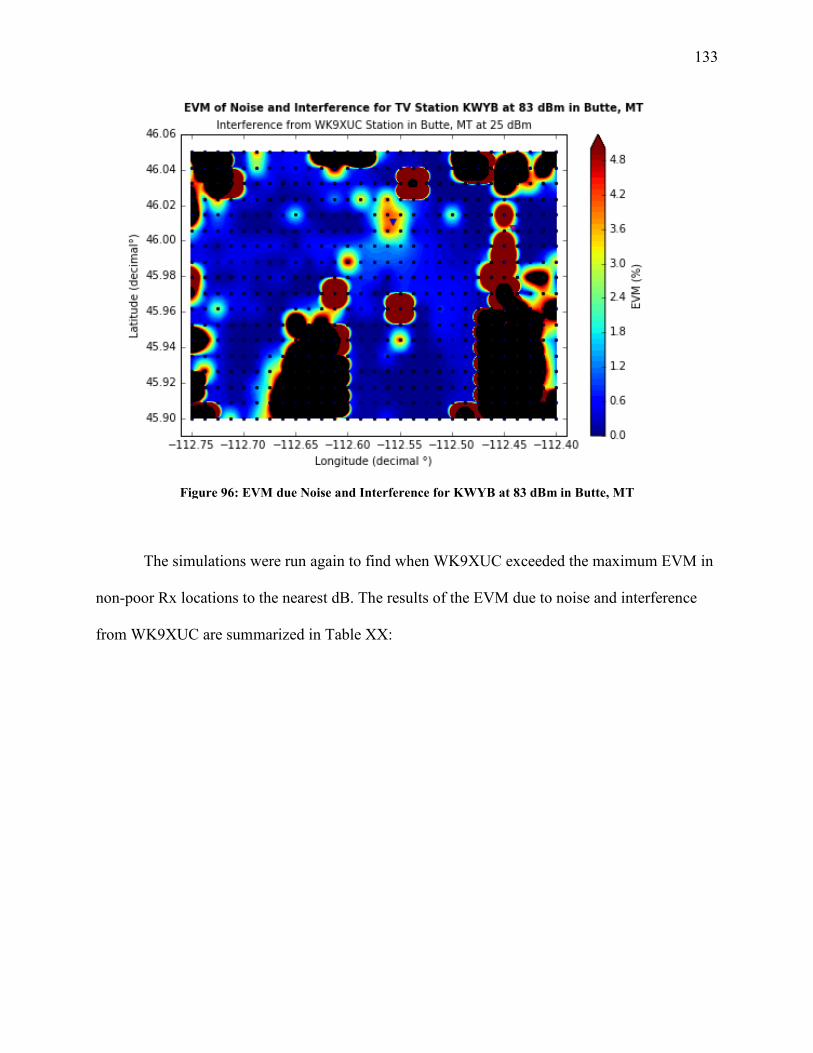
133

Figure 96: EVM due Noise and Interference for KWYB at 83 dBm in Butte, MT

The simulations were run again to find when WK9XUC exceeded the maximum EVM in

non-poor Rx locations to the nearest dB. The results of the EVM due to noise and interference

from WK9XUC are summarized in Table XX:

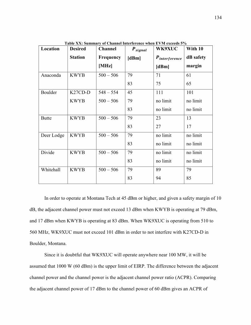
134

Table XX: Summary of Channel Interference when EVM exceeds 5% Location Desired

Station

Channel

Frequency

[MHz]

𝑷𝑷𝑵𝑵𝒃𝒃𝒈𝒈𝒃𝒃𝒃𝒃𝒎𝒎

[dBm]

WK9XUC

𝑷𝑷𝒃𝒃𝒃𝒃𝒕𝒕𝒃𝒃𝒍𝒍𝟐𝟐𝒃𝒃𝒍𝒍𝒃𝒃𝒃𝒃𝒄𝒄𝒃𝒃

[dBm]

With 10

dB safety

margin

Anaconda KWYB 500 – 506 79

83

71

75

61

65

Boulder K27CD-D

KWYB

548 – 554

500 – 506

45

79

83

111

no limit

no limit

101

no limit

no limit

Butte KWYB 500 – 506 79

83

23

27

13

17

Deer Lodge KWYB 500 – 506 79

83

no limit

no limit

no limit

no limit

Divide KWYB 500 – 506 79

83

no limit

no limit

no limit

no limit

Whitehall KWYB 500 – 506 79

83

89

94

79

85

In order to operate at Montana Tech at 45 dBm or higher, and given a safety margin of 10

dB, the adjacent channel power must not exceed 13 dBm when KWYB is operating at 79 dBm,

and 17 dBm when KWYB is operating at 83 dBm. When WK9XUC is operating from 510 to

560 MHz, WK9XUC must not exceed 101 dBm in order to not interfere with K27CD-D in

Boulder, Montana.

Since it is doubtful that WK9XUC will operate anywhere near 100 MW, it will be

assumed that 1000 W (60 dBm) is the upper limit of EIRP. The difference between the adjacent

channel power and the channel power is the adjacent channel power ratio (ACPR). Comparing

the adjacent channel power of 17 dBm to the channel power of 60 dBm gives an ACPR of

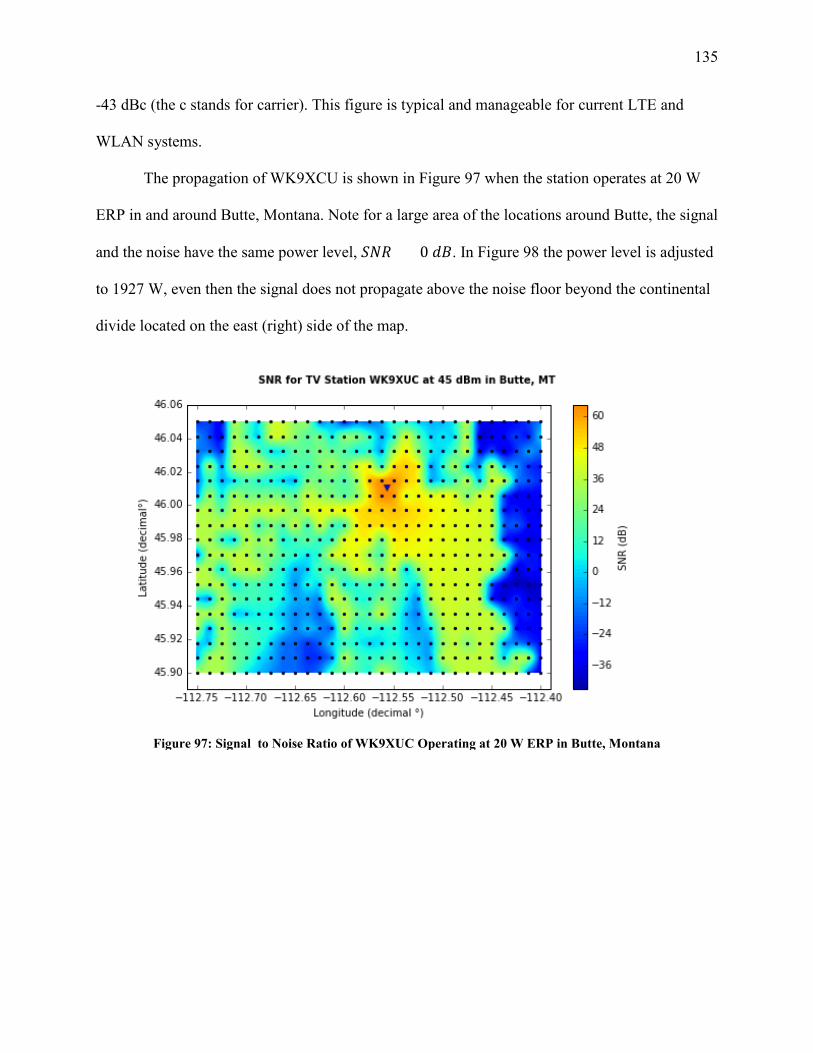
135

-43 dBc (the c stands for carrier). This figure is typical and manageable for current LTE and

WLAN systems.

The propagation of WK9XCU is shown in Figure 97 when the station operates at 20 W

ERP in and around Butte, Montana. Note for a large area of the locations around Butte, the signal

and the noise have the same power level, 𝑆𝑆𝑁𝑁𝑅𝑅 = 0 𝑑𝑑𝑑𝑑. In Figure 98 the power level is adjusted

to 1927 W, even then the signal does not propagate above the noise floor beyond the continental

divide located on the east (right) side of the map.

Figure 97: Signal to Noise Ratio of WK9XUC Operating at 20 W ERP in Butte, Montana

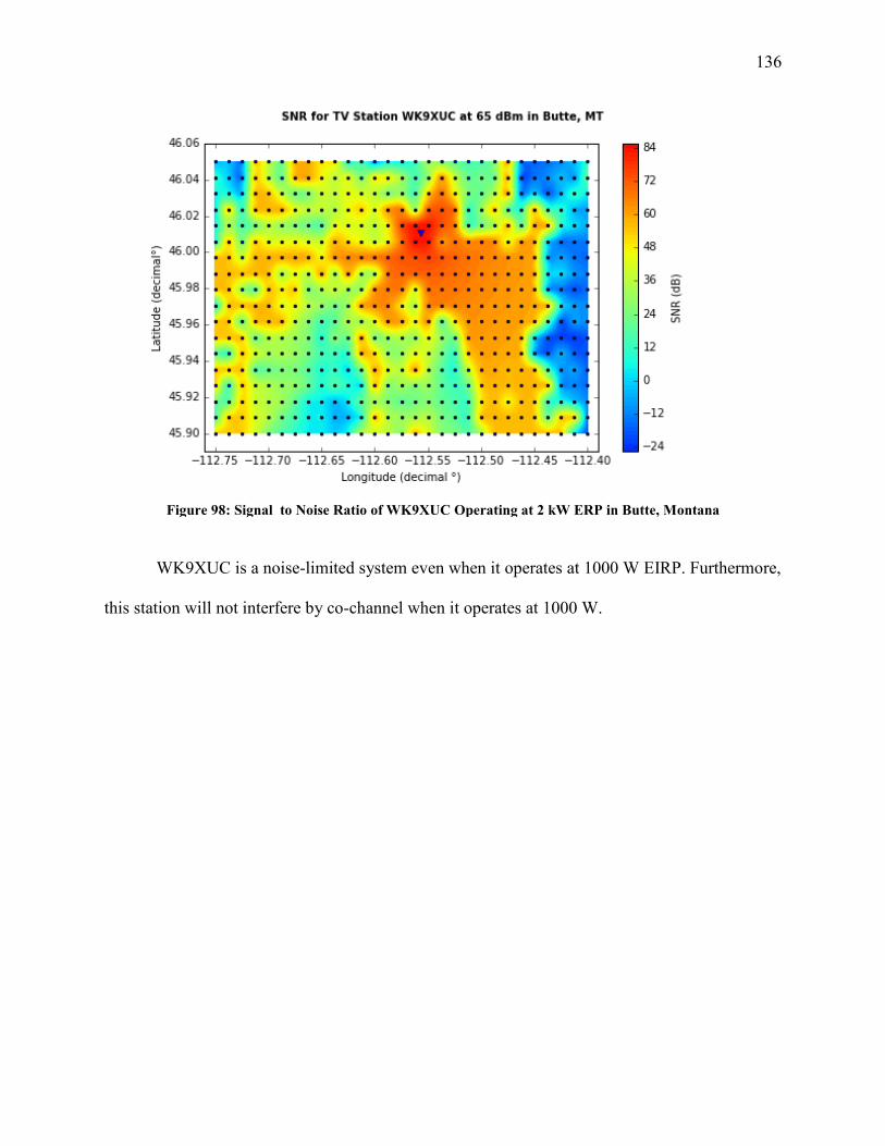
136

Figure 98: Signal to Noise Ratio of WK9XUC Operating at 2 kW ERP in Butte, Montana

WK9XUC is a noise-limited system even when it operates at 1000 W EIRP. Furthermore,

this station will not interfere by co-channel when it operates at 1000 W.

137

6. Conclusion

In many respects, this work demonstrates that there is an abundance of completely

underutilized spectrum available to provide mobile broadband communications in rural and

remote area located in western Montana. By monitoring the spectrum from 174 to 1000 MHz at

two locations, specifically at Montana Tech in Butte, Montana and a Moose Lake Road near

Philipsburg, Montana for a minimum of 2 weeks, spectrum use can be quantified. This work

characterizes the spectrum use across the span of interest by targeting 5-MHz channels. Each

channel is characterized by occupancy percentage, mean shift and maximum power.

There are many channels available for sharing across the span from 174 to 1000 MHz,

including but not limited to the spurious emissions dominated channels from 174 to 200 MHz,

channels from 510 to 550 MHz and the ISM band from 902 to 928 MHz. However, the 500 MHz

band is likely the best candidate for testing a rural broadband communications system. This is

because of the interference from spurious emission below 500 MHz and the interference, which

will likely occur, in the ISM band.

To design a rural broadband mobile communication system that optimizes coverage over

capacity in mountainous terrain, this work models a cellular base station that operates in Butte,

Montana. The Wireless Lab at Montana Tech was granted an experimental license to operate a

20 W ERP station, WK9XUC, in the 500 MHz band. The ITM was implemented to study the

propagation and various interference scenarios of this station, WK9XUC, with other TV stations.

This work demonstrates that cellular base station operating from 20 W to 1000 W in the 500

MHz band is viable from an interference point of view. Furthermore, WK9XUC is noise-limited

because the mountainous terrain block signals at given height, power and location.

138

References Cited

[1] M. Alleven. (2016, July 14). FCC OKs sweeping Spectrum Frontiers rules to open up

nearly 11 GHz of spectrum [Online]. Available: http://www.fiercewireless.com/tech/fcc-oks-

sweeping-spectrum-frontiers-rules-to-open-up-nearly-11-ghz-spectrum

[2] 5G [Online]. Available: https://en.wikipedia.org/wiki/5G

[3] S. Segan. (2015, June 15). 3G v. 4G speeds [Online]. Available:

http://www.pcmag.com/article/345123/fastest-mobile-networks-2016/4

[4] A. M. Kovacs. (2014, May 1). Regulation in financial translation: Will the incentive

auction increase mobile-broadband competition in rural America? [Online]. Available:

http://cbpp.georgetown.edu/publications/will-incentive-auction-increase-mobile-broadband-

competition-rural-america

[5] Spectrum Wiki. Standard LTE bands [Online]. Available:

http://www.spectrumwiki.com/Index.aspx

[6] Federal Communications Commission. (2014, May 15). Staff summary of incentive

auction report and order [Online]. Available: https://www.fcc.gov/document/staff-summary-

incentive-auction-report-and-order

[7] J. Engebretson. (2015, July 16). FCC adopts rural carrier bidding credit for 600 MHz

auction, delays other key issues [Online]. Available: http://www.telecompetitor.com/fcc-adopts-

rural-carrier-bidding-credit-for-600-mhz-auction-delays-other-key-issues/

[8] D. Meyer. (2016, October 19). FCC 600 MHz auction stage 2 ends after 1 round; On

to stage 3 [Online]. Available: http://www.rcrwireless.com/20161019/policy/fcc-600-mhz-

auction-stage-2-ends-1-round-stage-3-tag2

139

[9] M. Cotton et al., "An overview of the NTIA/NIST spectrum monitoring pilot

program," IEEE Wireless Communications and Networking Conf. Workshops (WCNCW), New

Orleans, LA, 2015, pp. 217-222. doi: 10.1109/WCNCW.2015.7122557

[10] Shared Spectrum Company. Spectrum reports [Online]. Available:

http://www.sharedspectrum.com/papers/spectrum-reports/

[11] R. Aguilar-Gonzalez, M. Cardenas-Juarez, U. Pineda-Rico and E. Stevens-Navarro,

"Spectrum Occupancy Measurements below 1 GHz in the City of San Luis Potosi, Mexico,"

IEEE 78th Vehicular Technology Conf. (VTC), Las Vegas, NV, 2013, pp. 1-5. doi:

10.1109/VTCFall.2013.6692420

[12] D. A. Roberson, C. S. Hood, J. L. LoCicero and J. T. MacDonald, "Spectral

Occupancy and Interference Studies in support of Cognitive Radio Technology Deployment," 1st

IEEE Workshop Networking Technologies for Software Defined Radio Networks, Reston, VA,

USA, 2006, pp. 26-35. doi: 10.1109/SDR.2006.4286323

[13] N. Faruk et al, “Large scale spectrum survey in rural and urban environments within

the 50 MHz-6 GHz bands,” Measurement, vol. 91, pp. 228-238, Sept. 2016.

[14] E. Wiles, B. Hill, F. A. da Silva and K. Negus, "Measurement and analysis of

spectrum occupancy from 140 to 1000 MHz in rural western Montana," 10th European Conf.

Antennas and Propagation (EuCAP), Davos, CH, 2016, pp. 1-4. doi:

10.1109/EuCAP.2016.7481328

[15] V. Valenta et al, "Survey on spectrum utilization in Europe: Measurements, analyses

and observations," Proc. 5th Int. Conf. Cognitive Radio Oriented Wireless Networks and

Communications, Cannes, FR, 2010, pp. 1-5. doi: 10.4108/ICST.CROWNCOM2010.9220

140

[16] S. D. Barnes, P. R. Botha, and B. T. Maharaj. “Spectral occupation of TV broadcast

bands: Measurement and analysis,” Measurement, vol. 93, pp. 272-277, Nov. 2016. doi:

10.1016/j.measurement.2016.07.020

[17] K. A. Qaraqe et al, “Measurement and analysis of wideband spectrum utilization in

indoor and outdoor environments,” 12th Int. Conf. Communications Technologies (ICCT),

Nanjing, CN, 2010. Available:

http://people.qatar.tamu.edu/khalid.qaraqe/KQPublications/icct10_v5.pdf

[18] M. Lopez-Benitez, A. Umbert and F. Casadevall, "Evaluation of Spectrum

Occupancy in Spain for Cognitive Radio Applications," IEEE 69th Vehicular Technology Conf.

(VTC), Barcelona, ES, 2009, pp. 1-5. doi: 10.1109/VETECS.2009.5073544

[19] R. Schiphorst and C. H. Slump, "Evaluation of Spectrum Occupancy in Amsterdam

Using Mobile Monitoring Vehicles," IEEE 71st Vehicular Technology Conf. (VTC), Taipei, TW,

2010, pp. 1-5. doi: 10.1109/VETECS.2010.5494056

[20] L. Mendes, L. Gonçalves and A. Gameiro, "GSM downlink spectrum occupancy

modeling," IEEE 22nd Int. Symp. Personal, Indoor and Mobile Radio Communications, Toronto,

ON, 2011, pp. 546-550. doi: 10.1109/PIMRC.2011.6140021

[21] S. Jayavalan, et al, “Measurements and analysis of spectrum occupancy in the

cellular and TV bands,” Lecture Notes on Software Engineering, vol. 2, no. 2, pp. 133-138, May

2014. doi: 10.7763/LNSE.2014.V2.110

[22] M. H. Islam et al., "Spectrum survey in Singapore: Occupancy measurements and

analyses," 3rd Int. Conf. Cognitive Radio Oriented Wireless Networks and Communications

(CROWNCOM), Singapore, 2008, pp. 1-7. doi: 10.1109/CROWNCOM.2008.4562457

141

[23] A. Marţian, C. Vlădeanu, I. Marcu, and I Marghescu, “Evaluation of spectrum

occupancy in an urban environment in a cognitive radio context,” International Journal on

Advances in Telecommunications, vol. 3, no. 3, pp. 172-181, 2010.

[24] S. W. Ellingson, "Spectral occupancy at VHF: implications for frequency-agile

cognitive radios," IEEE 62nd Vehicular Technology Conference (VTC), 2005, Dallas, TX, USA,

pp. 1379-1382. doi: 10.1109/VETECF.2005.1558153

[25] R. Attard et al., "A high-performance tiered storage system for a global spectrum

observatory network," 9th International Conference on Cognitive Radio Oriented Wireless

Networks and Communications (CROWNCOM), Oulu, FI, 2014, pp. 466-473. doi:

10.4108/icst.crowncom.2014.255740

[26] R. Urban, T. Korinek, and P. Pechac, “Broadband spectrum survey measurements

for cognitive radio applications,” Radioengineering, vol. 21, no. 4, pp. 1101-1109, 2012. doi:

10.13164/re.2012.1101

[27] S. Yin, D. Chen, Q. Zhang, M. Liu and S. Li, "Mining spectrum usage data: A large-

scale spectrum measurement study," IEEE Transactions on Mobile Computing, vol. 11, no. 6,

pp. 1033-1046, June 2012. doi: 10.1109/TMC.2011.128

[28] A. Petrin and P. G. Steffes, “Analysis and comparison of spectrum measurements

performed in urban and rural areas to determine the total amount of spectrum usage,” Proc. Int.

Symp. Advanced Radio Technologies (ISART), Boulder, CO, USA, 2005, pp. 9-12. Available:

https://www.its.bldrdoc.gov/publications/05-418.aspx

[29] C. A. Hammerschmidt, Heather E. Ottke, J. Randy Hoffman “Broadband spectrum

survey in the Denver area,” NTIA, Washington, DC, Rep. TR-13-496, 2013. Available:

https://www.its.bldrdoc.gov/publications/2735.aspx

142

[30] C. A. Hammerschmidt, “Broadband spectrum survey in the San Diego, California,

area,” NTIA, Washington, DC, Rep. TR-14-498, 2014. Available:

https://www.its.bldrdoc.gov/publications/2741.aspx

[31] C. A. Hammerschmidt “Broadband spectrum survey in the Chicago, Illinois, area,”

NTIA, Washington, DC, Rep. TR-14-502, 2014. Available:

https://www.its.bldrdoc.gov/publications/2756.aspx

[32] R. Bacchus, T. Taher, K. Zdunek and D. Roberson, "Spectrum utilization study in

support of dynamic spectrum access for public safety," IEEE Symp. New Frontiers Dynamic

Spectrum (DySPAN), Singapore, 2010, pp. 1-11. doi: 10.1109/DYSPAN.2010.5457871

[33] R. I. C. Chiang, G. B. Rowe and K. W. Sowerby, "A quantitative analysis of spectral

occupancy measurements for cognitive radio," IEEE 65th Vehicular Technology Conference

(VCT), Dublin, IE, 2007, pp. 3016-3020. doi: 10.1109/VETECS.2007.618

[34] M. Mehdawi, N. Riley, K. Paulson, A. Fanan, and M. Ammar, “Spectrum occupancy

survey in HULL-UK for cognitive radio applications: measurement & analysis,” International

Journal of Scientific & Technology Research, vol. 2, no. 4, pp. 231-236, Apr. 2013. Available:

http://www.ijstr.org/final-print/apr2013/Spectrum-Occupancy-Survey-In-Hull-uk-For-Cognitive-

Radio-Applications-Measurement-&-Analysis.pdf

[35] M. Wellens, J. Wu and P. Mahonen, "Evaluation of spectrum occupancy in indoor

and outdoor scenario in the context of cognitive radio," 2nd Int. Conf. Cognitive Radio Oriented

Wireless Networks and Communications, Orlando, FL, USA, 2007, pp. 420-427. doi:

10.1109/CROWNCOM.2007.4549835

143

[36] T. Harrold, R. Cepeda and M. Beach, "Long-term measurements of spectrum

occupancy characteristics," IEEE Int. Symp. Dynamic Spectrum Access Networks (DySPAN),

Aachen, DE, 2011, pp. 83-89. doi: 10.1109/DYSPAN.2011.5936272

[37] OpenSignal. OpenSignal app [Online]. Available: https://opensignal.com/

[38] OpenSignal. The state of LTE [Online]. (2016, February). Available:

https://opensignal.com/reports/2016/02/state-of-lte-q4-2015/

[39] OpenSignal. Compare mobile networks near you [Online]. (2017, May). Available:

https://opensignal.com/coverage-maps/

[40] A. G. Longley and P. L. Rice, “Prediction of tropospheric radio transmission loss

over irregular terrain. A computer method-1968,” ITS, Boulder, CO, Rep. ITS-67, 1968.

Available: https://www.its.bldrdoc.gov/publications/download/ERL%2079-ITS%2067.pdf

[41] Borb – Wikimedia Commons. Inverse square law [Image]. Available:

https://commons.wikimedia.org/w/index.php?curid=3816716

[42] Agilent Technologies. Spectrum analysis basics [Online]. Available:

http://cp.literature.agilent.com/litweb/pdf/5952-0292.pdf

[43] Berkeley Nucleonics Corp. RTSA7500 programmer’s manual (v3.6.2) [Online].

Available:

http://www.berkeleynucleonics.com/sites/berkeleynucleonics/files/products/manuals/model7500

_programmersmanual_ver3_6_2.pdf

[44] SciPy.org. NumPy Manual v1.12: Discrete Fourier Transform [Online]. Available:

https://docs.scipy.org/doc/numpy/reference/routines.fft.html

[45] Diamond Antenna. D3000N Super Discone Antenna [Online]. Available:

http://www.diamondantenna.net/d3000n.html

144

[46] RF Bay, Inc. LNA-1520 [Online]. Available:

http://rfbayinc.com/products_pdf/product_91.pdf

[47] COM-Power Corporation. PAM-103 [Online]. Available: http://www.com-

power.com/datasheets/PAM-103.pdf

[48] Tin Lee Electronics. Welcome to Tin Lee Electronics Ltd. [Online]. Available:

http://www.tinlee.com/index.php

[49] L-com. N-Male to N-Female Bulkhead 0-3 GHz Coaxial Lightning Protector

[Online]. Available: http://www.l-com.com/multimedia/datasheets/DS_AL-NMNFB-_.PDF

[50] Stridsberg Engineering, LLC. FLT201A specifications [Online]. Available:

http://www.stridsberg.com/prod02.htm

[51] Google Earth Pro. (2016). Map data: Landsat / Copernicus [Image].

[52] PyRF. PyRF documentation [Online]. Available:

https://pyrf.readthedocs.io/en/latest/

[53] R. Yarbough. TPI-1002-A Signal Generator [Online]. Available: http://www.rf-

consultant.com/tpi-1002-a-signal-generator/

[54] Reuex Industrial Co., Ltd. (Nagoya Antenna). Handheld Antenna NA-771, 144/430

MHz [Online]. Available: http://www.nagoya.com.tw/en/2-2277-66883/product/NA-771-

id384799.html

[55] Keysight Technologies. 8753E RF Network Analyzer, 30 kHz to 3 or 6 GHz

[Online]. Available: http://www.keysight.com/en/pd-1000002294%3Aepsg%3Apro-pn-

8753E/rf-network-analyzer-30-khz-to-3-or-6-ghz?cc=US&lc=eng

[56] The Python Standard Library. 8.6. array — Efficient arrays of numeric values

[Online]. Available: https://docs.python.org/2/library/array.html

145

[57] Wireless Lab Montana Tech. YouTube Channel [Online]. Available:

https://www.youtube.com/channel/UC0Ywn5qi34CDN5lFf8Gmrgg

[58] MMX Technology, LCC. Spectrum Wiki [Online]. Available:

http://www.spectrumwiki.com/Index.aspx

[59] Federal Communications Commission. (2017, March 26). TV Query of stations

located within 141 km of Butte, MT [Online]. Available: https://transition.fcc.gov/fcc-

bin/tvq?state=MT&call=&arn=&city=&chan=&cha2=69&serv=&type=0&facid=&asrn=&list=1

&dist=&dlat2=&mlat2=&slat2=&dlon2=&mlon2=&slon2=&size=9

[60] REC Networks. FCCdata.org [Online]. Available: https://fccdata.org/

[61] SatelliteGuys. RabbitEars [Online]. Available: http://www.rabbitears.info/

[62] J. Maglicane. SPLAT! A terrestrial RF path analysis application for LINUX/UNIX

[Online]. Available: http://www.qsl.net/kd2bd/splat.html

[63] USGS. SRTM database [Online]. Available: https://dds.cr.usgs.gov/srtm/

[64] S. Kasampalis et al, “Comparison of Longley-Rice, ITM and ITWOM propagation

models for DTV and FM broadcasting,” 16th Int. Symp. Wireless Personal Multimedia

Communications (WPMC), Atlantic City, NJ, USA, 2013, pp. 1-6. Available:

http://ieeexplore.ieee.org/document/6618611/

[65] The Math Forum at NCTM. (1999, April 20). Deriving the Haversine formula

[Online]. Available: http://mathforum.org/library/drmath/view/51879.html

[66] A. McGovern. Geographic distance and azimuth calculations [Online]. Available:

http://www.codeguru.com/cpp/cpp/algorithms/article.php/c5115/Geographic-Distance-and-

Azimuth-Calculations.htm

146

[67] USGS. Region definition [Image]. Available:

https://dds.cr.usgs.gov/srtm/version2_1/SRTM1/Region_definition.jpg

[68] USGS. Continent definition [Image]. Available:

https://dds.cr.usgs.gov/srtm/version2_1/Documentation/Continent_def.gif

[69] G. A. Hufford, A. G. Longley, W. A. & Kissick, “A guide to the use of the ITS

irregular terrain model in the area prediction mode,” NTIA, Washington, DC, Rep. 82-100, 1982.

Available: https://www.ntia.doc.gov/files/ntia/publications/ntia_82-

100_20121129145031_555510.pdf

[70] ITU Radiocommunication Sector, “The radio refractive index: its formula and

refractivity data,” ITU, Geneva, CH, 2015. Available: https://www.itu.int/dms_pubrec/itu-

r/rec/p/R-REC-P.453-11-201507-S!!PDF-E.pdf

[71] G. A. Hufford, “The ITS irregular terrain model, version 1.2.2 – The algorithm,”

NTIA, Boulder, CO, 1984. Available: https://www.its.bldrdoc.gov/media/50676/itm_alg.pdf

[72] B. R. Bean, J. D. Horn and A. M. Ozanich, NBS Monograph 22: Climatic charts and

data of the radio refractive index for the United States and the World. Washington, DC: U.S.

Government Printing Office, 1960. Available:

http://digicoll.manoa.hawaii.edu/techreports/PDF/NBS22.pdf

[73] JeffConrad – Wikimedia Commons. Geometric distance to horizon [Image].

Available: https://commons.wikimedia.org/w/index.php?curid=14958770

[74] J. D. Hunter, “Matplotlib: A 2D graphics environment,” Computing in Science &

Engineering, vol. 9, no. 3, pp. 90-95, 2007. doi: 10.1109/MCSE.2007.55

[75] Delaunay triangulation [Online]. Available:

https://en.wikipedia.org/wiki/Delaunay_triangulation

147

[76] J. Whitaker. (2010, July 30). NCAR natgrid library [Online]. Available:

https://github.com/matplotlib/natgrid

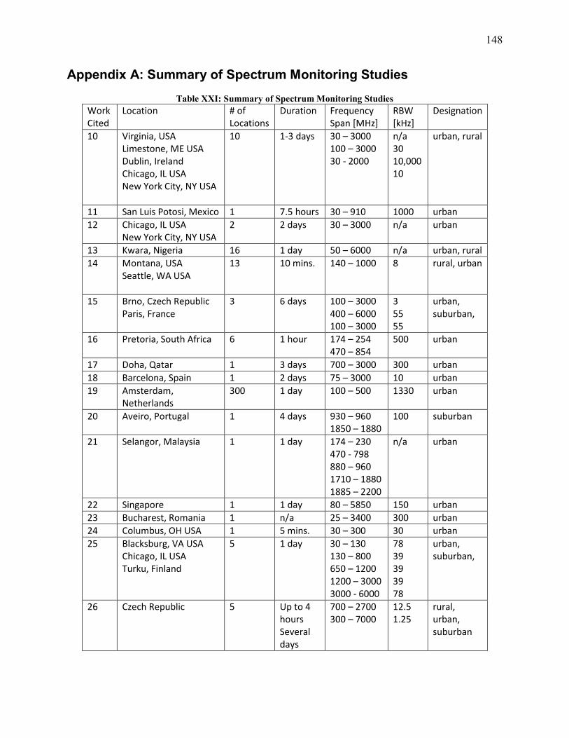
148

Appendix A: Summary of Spectrum Monitoring Studies Table XXI: Summary of Spectrum Monitoring Studies

Work Cited

Location # of Locations

Duration Frequency Span [MHz]

RBW [kHz]

Designation

10 Virginia, USA Limestone, ME USA Dublin, Ireland Chicago, IL USA New York City, NY USA

10 1-3 days 30 – 3000 100 – 3000 30 - 2000

n/a 30 10,000 10

urban, rural

11 San Luis Potosi, Mexico 1 7.5 hours 30 – 910 1000 urban 12 Chicago, IL USA

New York City, NY USA 2 2 days 30 – 3000 n/a urban

13 Kwara, Nigeria 16 1 day 50 – 6000 n/a urban, rural 14 Montana, USA

Seattle, WA USA

13 10 mins. 140 – 1000 8 rural, urban

15 Brno, Czech Republic Paris, France

3 6 days 100 – 3000 400 – 6000 100 – 3000

3 55 55

urban, suburban,

16 Pretoria, South Africa 6 1 hour 174 – 254 470 – 854

500 urban

17 Doha, Qatar 1 3 days 700 – 3000 300 urban 18 Barcelona, Spain 1 2 days 75 – 3000 10 urban 19 Amsterdam,

Netherlands 300 1 day 100 – 500 1330 urban

20 Aveiro, Portugal 1 4 days 930 – 960 1850 – 1880

100 suburban

21 Selangor, Malaysia 1 1 day 174 – 230 470 - 798 880 – 960 1710 – 1880 1885 – 2200

n/a urban

22 Singapore 1 1 day 80 – 5850 150 urban 23 Bucharest, Romania 1 n/a 25 – 3400 300 urban 24 Columbus, OH USA 1 5 mins. 30 – 300 30 urban 25 Blacksburg, VA USA

Chicago, IL USA Turku, Finland

5 1 day 30 – 130 130 – 800 650 – 1200 1200 – 3000 3000 - 6000

78 39 39 39 78

urban, suburban,

26 Czech Republic 5 Up to 4 hours Several days

700 – 2700 300 – 7000

12.5 1.25

rural, urban, suburban

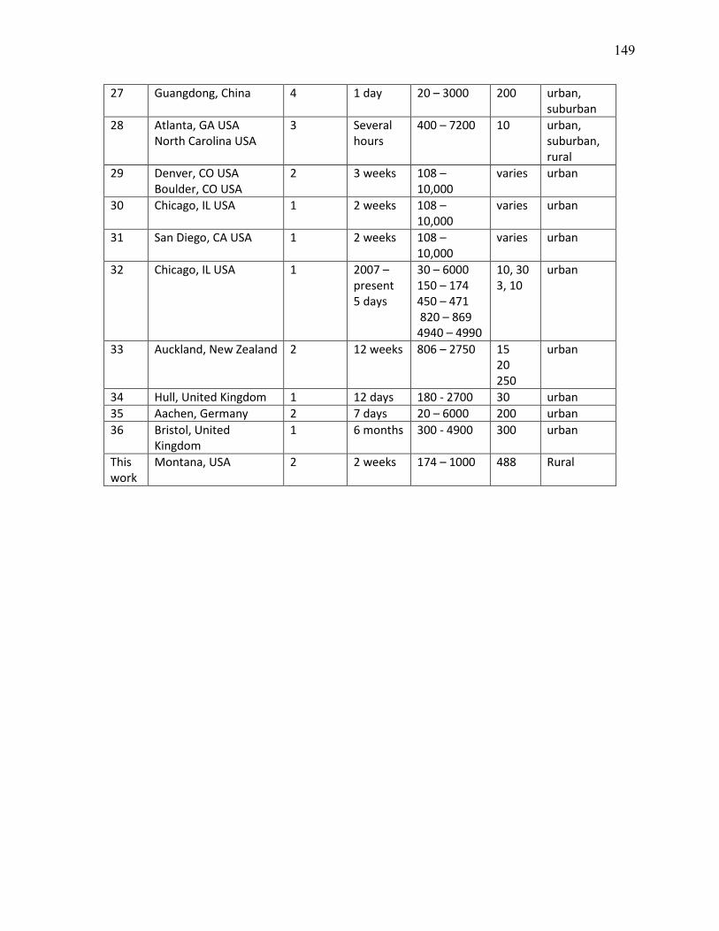
149

27 Guangdong, China 4 1 day 20 – 3000 200 urban, suburban

28 Atlanta, GA USA North Carolina USA

3 Several hours

400 – 7200

10 urban, suburban, rural

29 Denver, CO USA Boulder, CO USA

2 3 weeks 108 – 10,000

varies urban

30 Chicago, IL USA 1 2 weeks 108 – 10,000

varies urban

31 San Diego, CA USA 1 2 weeks 108 – 10,000

varies urban

32 Chicago, IL USA 1 2007 – present 5 days

30 – 6000 150 – 174 450 – 471 820 – 869 4940 – 4990

10, 30 3, 10

urban

33 Auckland, New Zealand 2 12 weeks 806 – 2750 15 20 250

urban

34 Hull, United Kingdom 1 12 days 180 - 2700 30 urban 35 Aachen, Germany 2 7 days 20 – 6000 200 urban 36 Bristol, United

Kingdom 1 6 months 300 - 4900 300 urban

This work

Montana, USA 2 2 weeks 174 – 1000 488 Rural

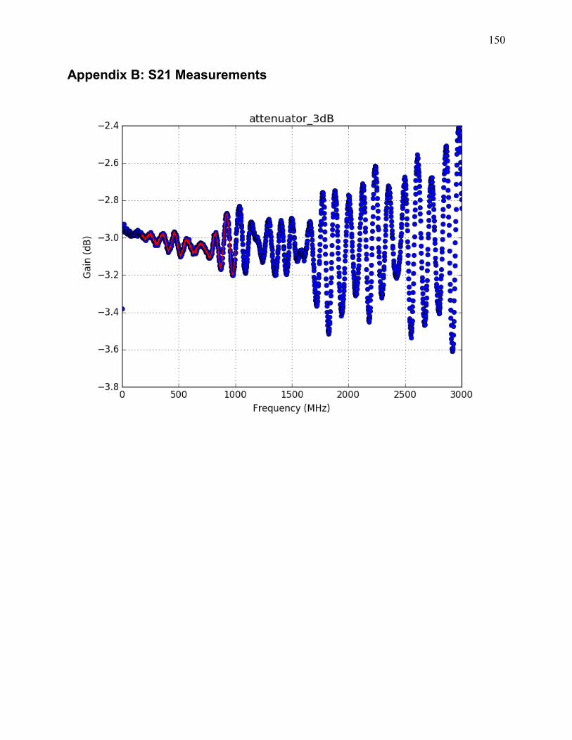
150

Appendix B: S21 Measurements

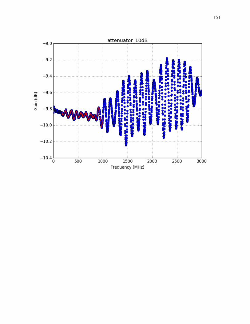
151

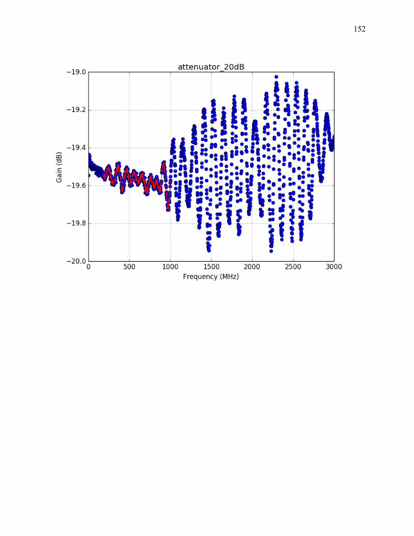
152

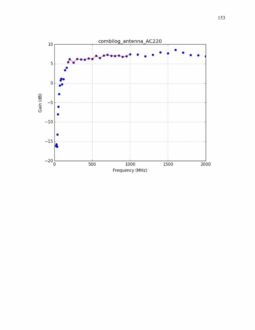
153

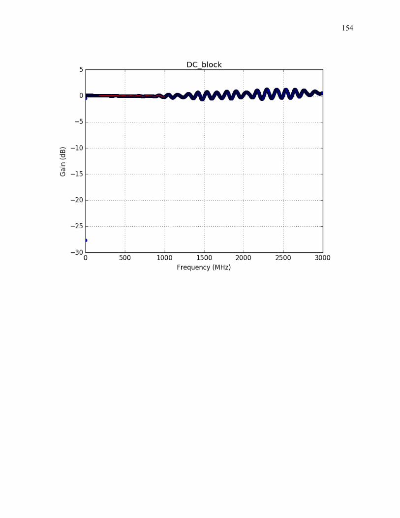
154

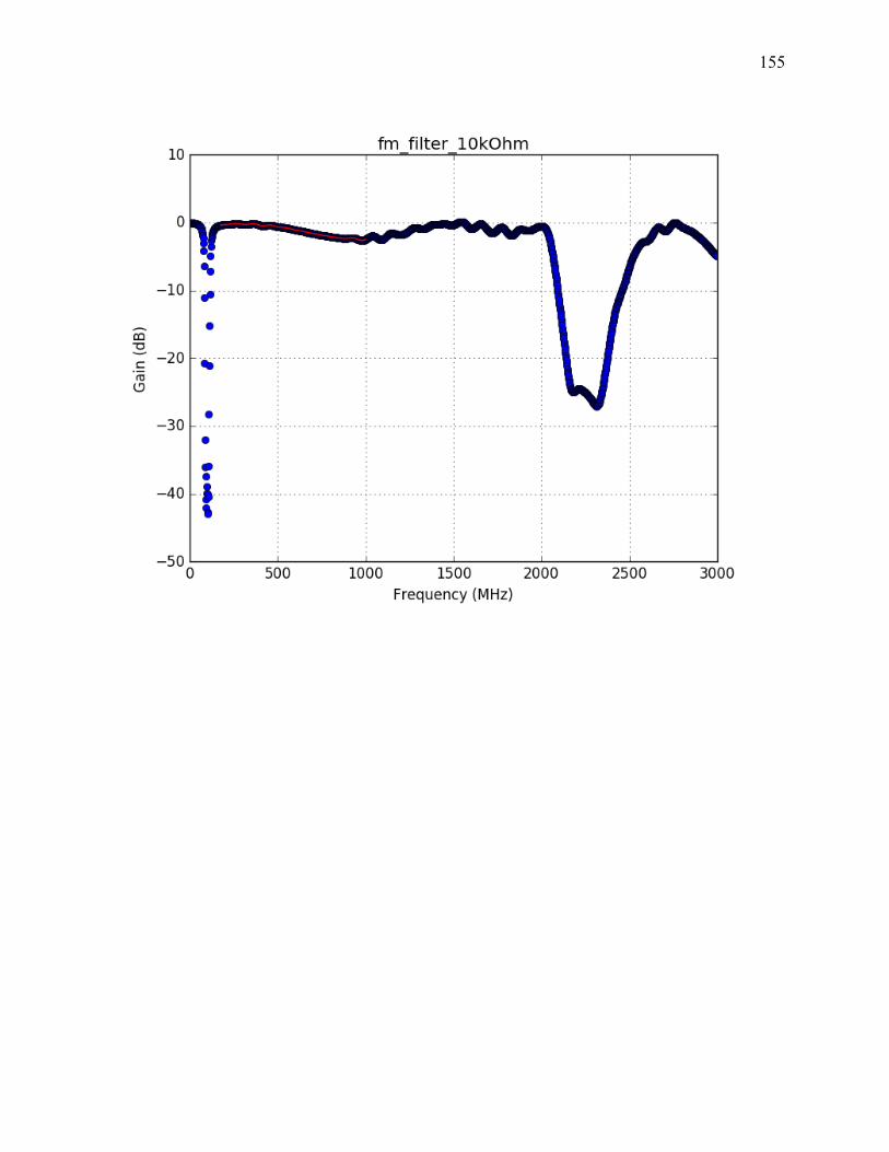
155

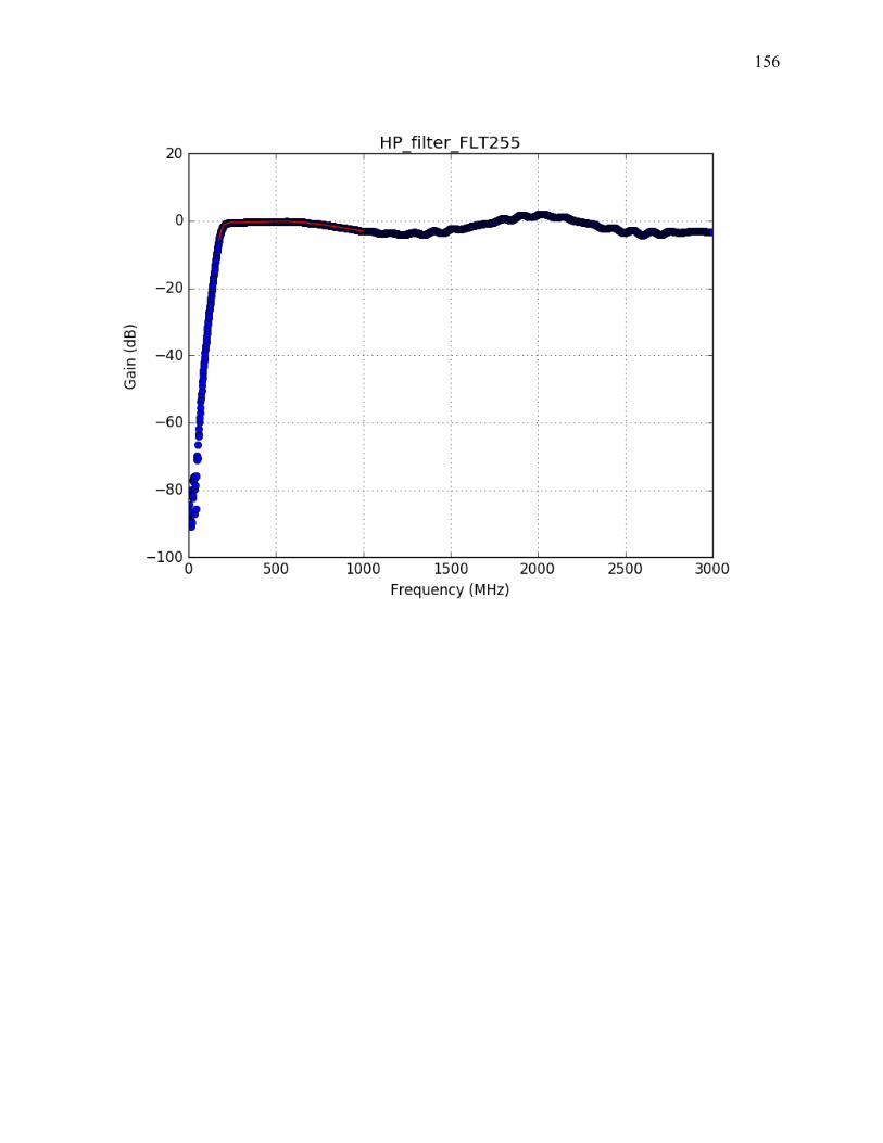
156

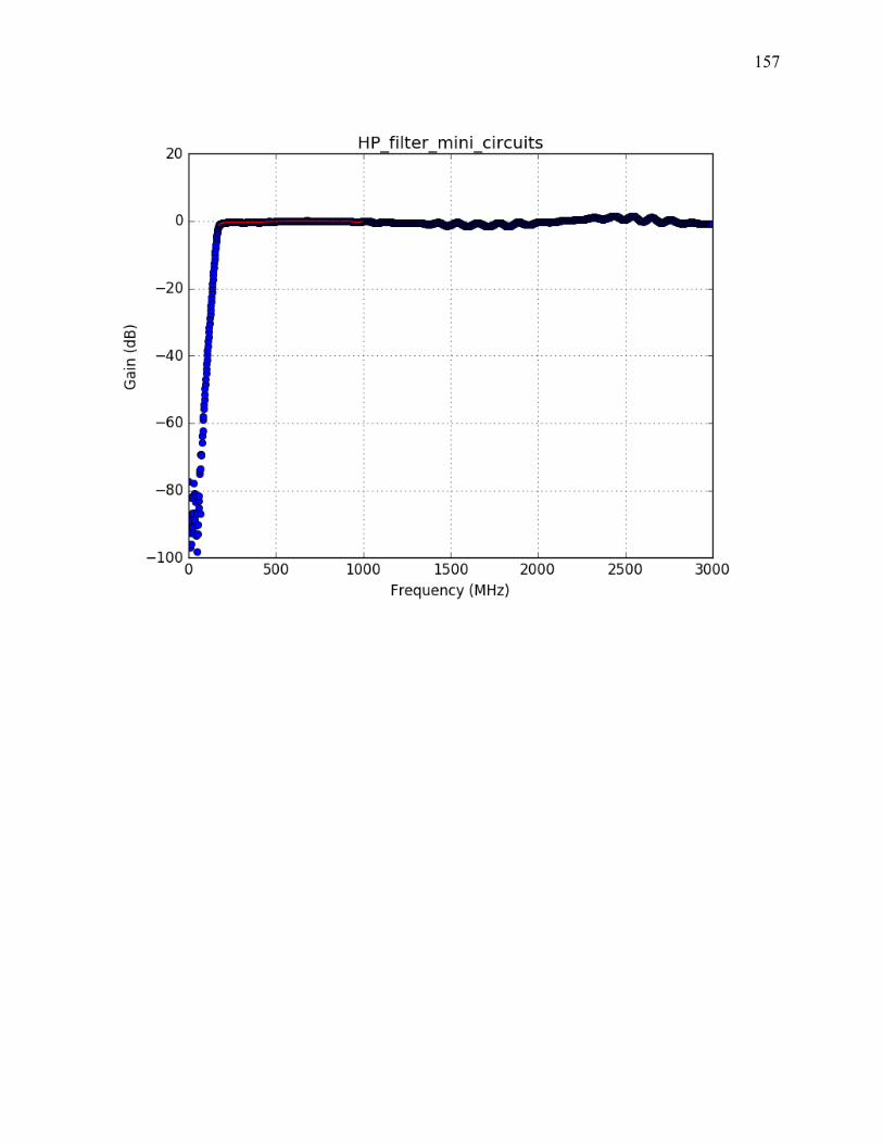
157

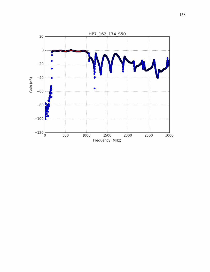
158

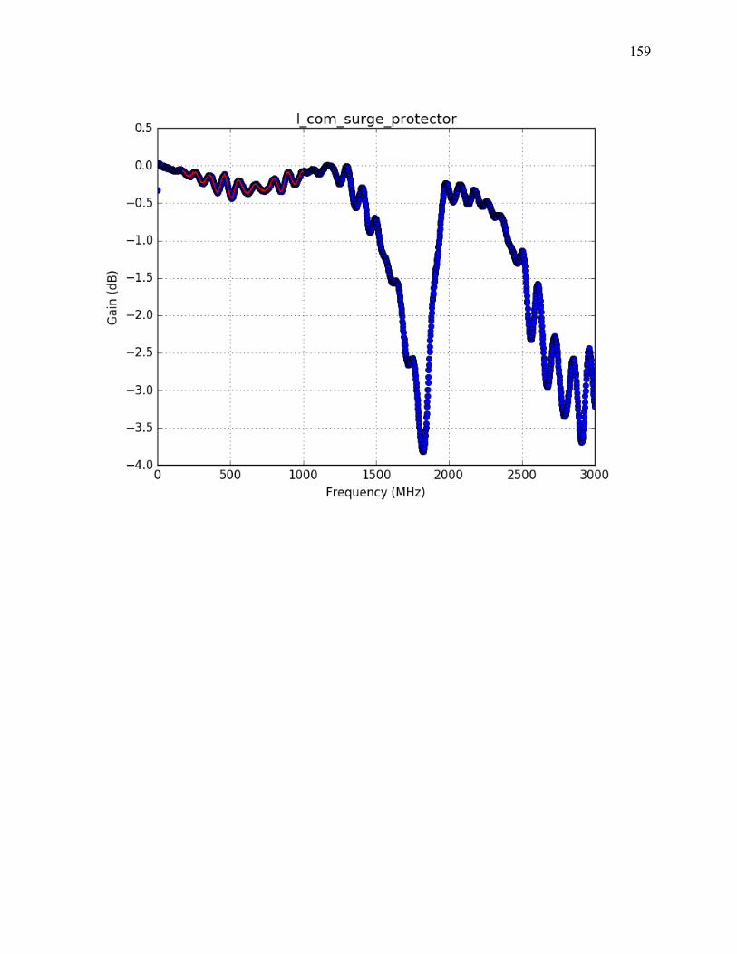
159

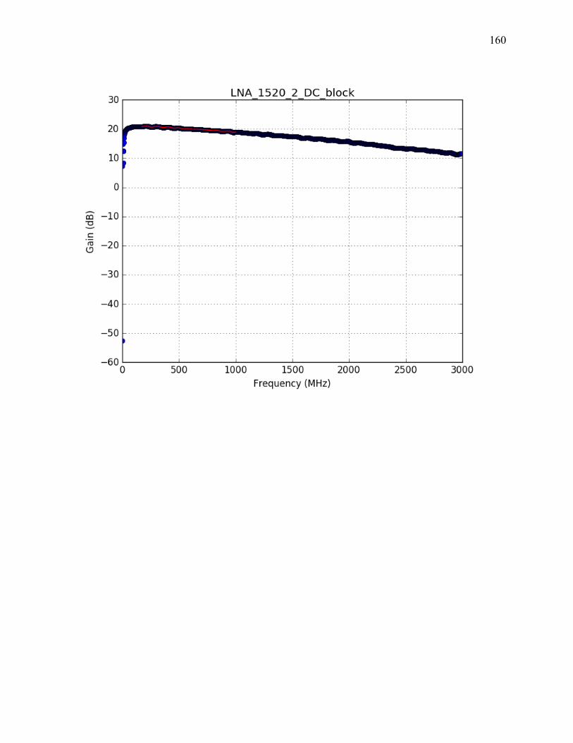
160

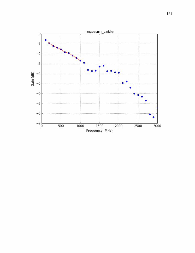
161

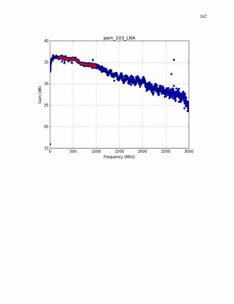
162

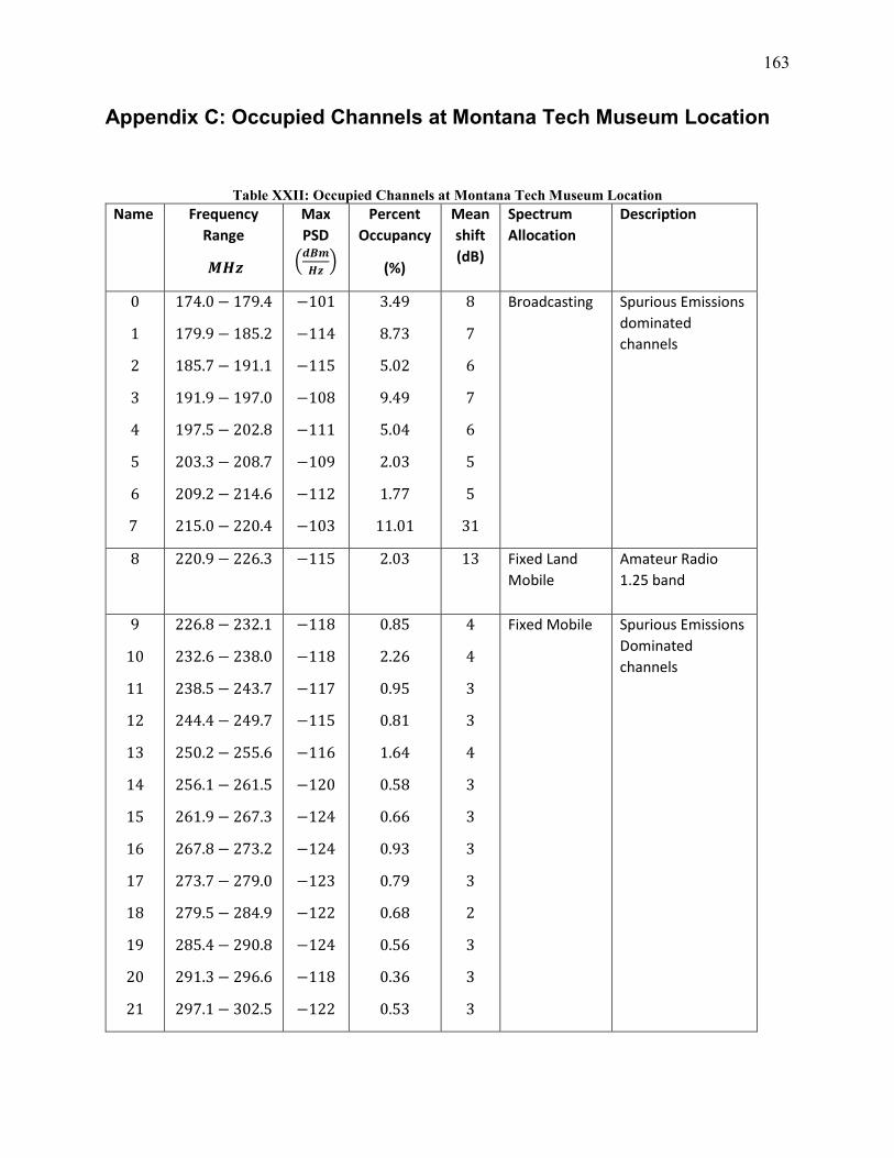
163

Appendix C: Occupied Channels at Montana Tech Museum Location

Table XXII: Occupied Channels at Montana Tech Museum Location Name Frequency

Range

(𝑴𝑴𝑯𝑯𝑯𝑯)

Max PSD

�𝒃𝒃𝒅𝒅𝒎𝒎𝑯𝑯𝑯𝑯

�

Percent Occupancy

(%)

Mean shift (dB)

Spectrum Allocation

Description

0

1

2

3

4

5

6

7

174.0 − 179.4

179.9− 185.2

185.7− 191.1

191.9− 197.0

197.5− 202.8

203.3− 208.7

209.2− 214.6

215.0 − 220.4

−101

−114

−115

−108

−111

−109

−112

−103

3.49

8.73

5.02

9.49

5.04

2.03

1.77

11.01

8

7

6

7

6

5

5

31

Broadcasting

Spurious Emissions dominated channels

8

220.9− 226.3 −115

2.03

13 Fixed Land Mobile

Amateur Radio 1.25 band

9

10

11

12

13

14

15

16

17

18

19

20

21

226.8 − 232.1

232.6− 238.0

238.5− 243.7

244.4− 249.7

250.2− 255.6

256.1 − 261.5

261.9− 267.3

267.8 − 273.2

273.7− 279.0

279.5− 284.9

285.4− 290.8

291.3− 296.6

297.1 − 302.5

−118

−118

−117

−115

−116

−120

−124

−124

−123

−122

−124

−118

−122

0.85

2.26

0.95

0.81

1.64

0.58

0.66

0.93

0.79

0.68

0.56

0.36

0.53

4

4

3

3

4

3

3

3

3

2

3

3

3

Fixed Mobile

Spurious Emissions Dominated channels

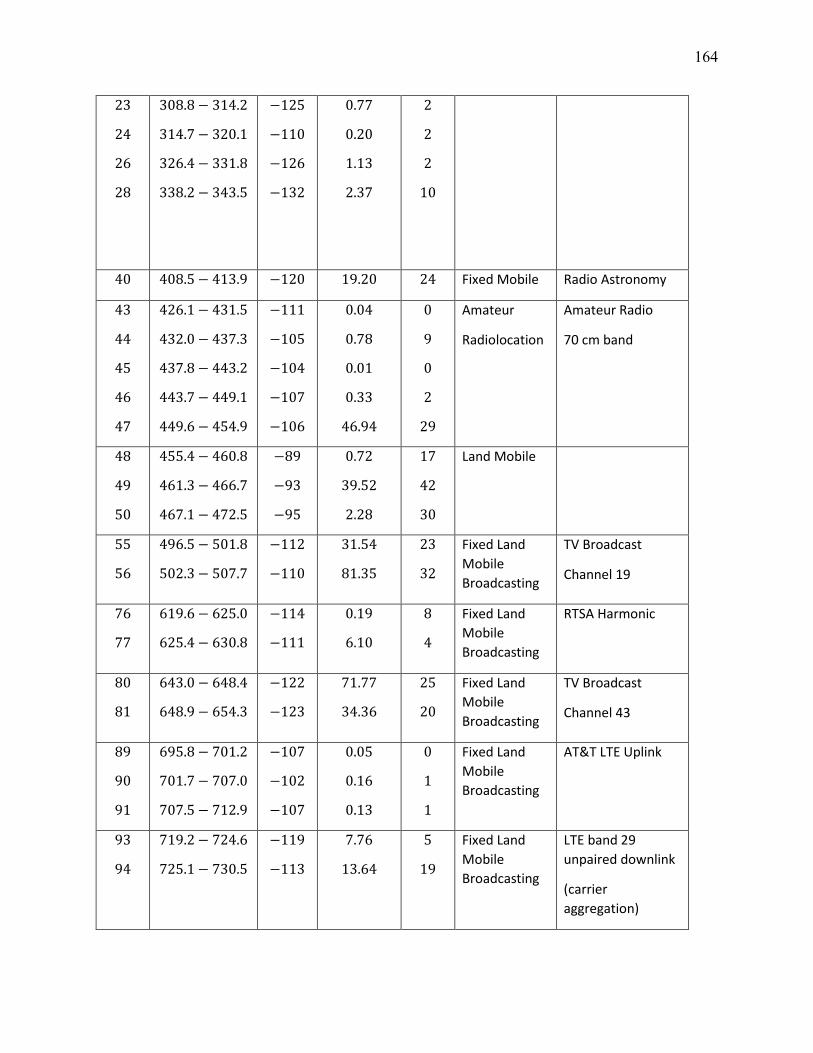
164

23

24

26

28

308.8 − 314.2

314.7− 320.1

326.4− 331.8

338.2− 343.5

−125

−110

−126

−132

0.77

0.20

1.13

2.37

2

2

2

10

40 408.5− 413.9 −120 19.20 24 Fixed Mobile Radio Astronomy

43

44

45

46

47

426.1 − 431.5

432.0 − 437.3

437.8 − 443.2

443.7− 449.1

449.6− 454.9

−111

−105

−104

−107

−106

0.04

0.78

0.01

0.33

46.94

0

9

0

2

29

Amateur

Radiolocation

Amateur Radio

70 cm band

48

49

50

455.4− 460.8

461.3− 466.7

467.1 − 472.5

−89

−93

−95

0.72

39.52

2.28

17

42

30

Land Mobile

55

56

496.5− 501.8

502.3− 507.7

−112

−110

31.54

81.35

23

32

Fixed Land Mobile Broadcasting

TV Broadcast

Channel 19

76

77

619.6− 625.0

625.4− 630.8

−114

−111

0.19

6.10

8

4

Fixed Land Mobile Broadcasting

RTSA Harmonic

80

81

643.0 − 648.4

648.9− 654.3

−122

−123

71.77

34.36

25

20

Fixed Land Mobile Broadcasting

TV Broadcast

Channel 43

89

90

91

695.8 − 701.2

701.7− 707.0

707.5− 712.9

−107

−102

−107

0.05

0.16

0.13

0

1

1

Fixed Land Mobile Broadcasting

AT&T LTE Uplink

93

94

719.2− 724.6

725.1 − 730.5

−119

−113

7.76

13.64

5

19

Fixed Land Mobile Broadcasting

LTE band 29 unpaired downlink

(carrier aggregation)

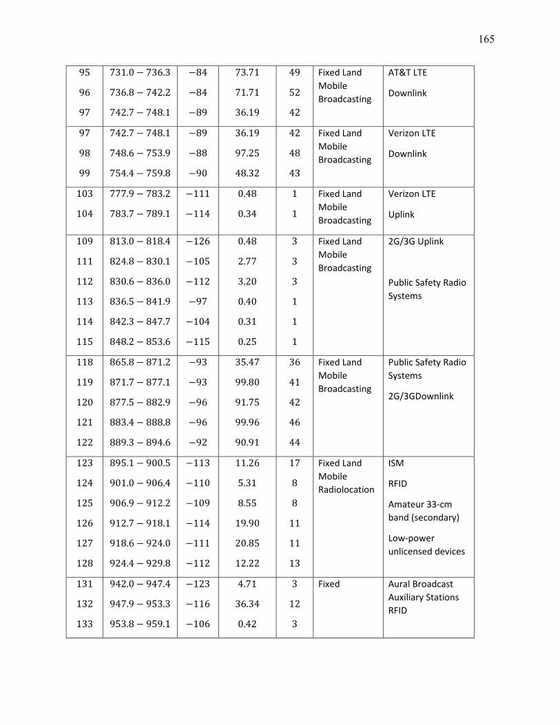
165

95

96

97

731.0 − 736.3

736.8 − 742.2

742.7− 748.1

−84

−84

−89

73.71

71.71

36.19

49

52

42

Fixed Land Mobile Broadcasting

AT&T LTE

Downlink

97

98

99

742.7− 748.1

748.6− 753.9

754.4− 759.8

−89

−88

−90

36.19

97.25

48.32

42

48

43

Fixed Land Mobile Broadcasting

Verizon LTE

Downlink

103

104

777.9− 783.2

783.7− 789.1

−111

−114

0.48

0.34

1

1

Fixed Land Mobile Broadcasting

Verizon LTE

Uplink

109

111

112

113

114

115

813.0 − 818.4

824.8 − 830.1

830.6− 836.0

836.5− 841.9

842.3− 847.7

848.2− 853.6

−126

−105

−112

−97

−104

−115

0.48

2.77

3.20

0.40

0.31

0.25

3

3

3

1

1

1

Fixed Land Mobile Broadcasting

2G/3G Uplink

Public Safety Radio Systems

118

119

120

121

122

865.8 − 871.2

871.7− 877.1

877.5− 882.9

883.4− 888.8

889.3− 894.6

−93

−93

−96

−96

−92

35.47

99.80

91.75

99.96

90.91

36

41

42

46

44

Fixed Land Mobile Broadcasting

Public Safety Radio Systems

2G/3GDownlink

123

124

125

126

127

128

895.1 − 900.5

901.0 − 906.4

906.9− 912.2

912.7− 918.1

918.6− 924.0

924.4− 929.8

−113

−110

−109

−114

−111

−112

11.26

5.31

8.55

19.90

20.85

12.22

17

8

8

11

11

13

Fixed Land Mobile Radiolocation

ISM

RFID

Amateur 33-cm band (secondary)

Low-power unlicensed devices

131

132

133

942.0 − 947.4

947.9− 953.3

953.8 − 959.1

−123

−116

−106

4.71

36.34

0.42

3

12

3

Fixed Aural Broadcast Auxiliary Stations RFID

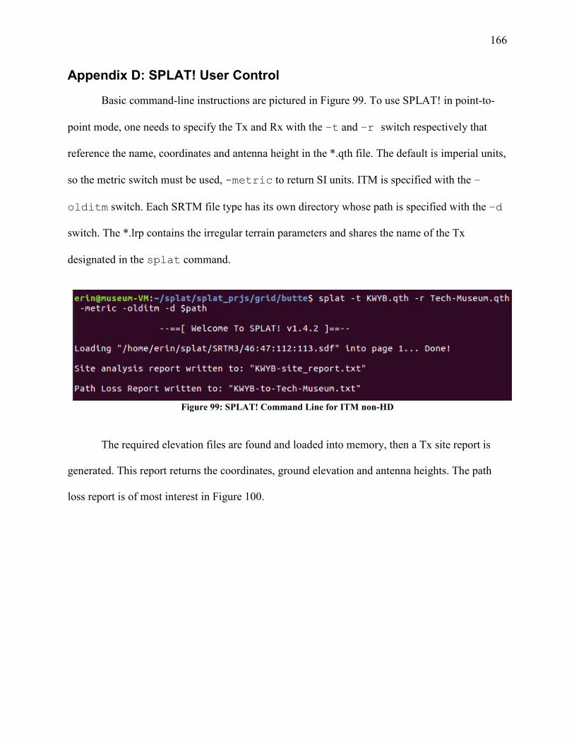
166

Appendix D: SPLAT! User Control

Basic command-line instructions are pictured in Figure 99. To use SPLAT! in point-to-

point mode, one needs to specify the Tx and Rx with the –t and –r switch respectively that

reference the name, coordinates and antenna height in the *.qth file. The default is imperial units,

so the metric switch must be used, -metric to return SI units. ITM is specified with the –

olditm switch. Each SRTM file type has its own directory whose path is specified with the –d

switch. The *.lrp contains the irregular terrain parameters and shares the name of the Tx

designated in the splat command.

Figure 99: SPLAT! Command Line for ITM non-HD

The required elevation files are found and loaded into memory, then a Tx site report is

generated. This report returns the coordinates, ground elevation and antenna heights. The path

loss report is of most interest in Figure 100.

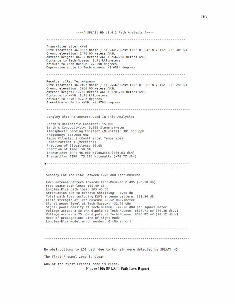
167

Figure 100: SPLAT! Path Loss Report

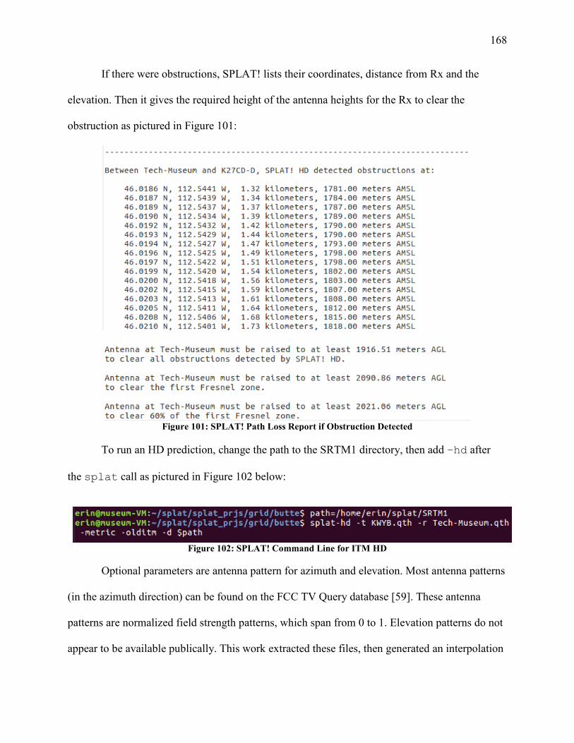
168

If there were obstructions, SPLAT! lists their coordinates, distance from Rx and the

elevation. Then it gives the required height of the antenna heights for the Rx to clear the

obstruction as pictured in Figure 101:

Figure 101: SPLAT! Path Loss Report if Obstruction Detected

To run an HD prediction, change the path to the SRTM1 directory, then add –hd after

the splat call as pictured in Figure 102 below:

Figure 102: SPLAT! Command Line for ITM HD

Optional parameters are antenna pattern for azimuth and elevation. Most antenna patterns

(in the azimuth direction) can be found on the FCC TV Query database [59]. These antenna

patterns are normalized field strength patterns, which span from 0 to 1. Elevation patterns do not

appear to be available publically. This work extracted these files, then generated an interpolation

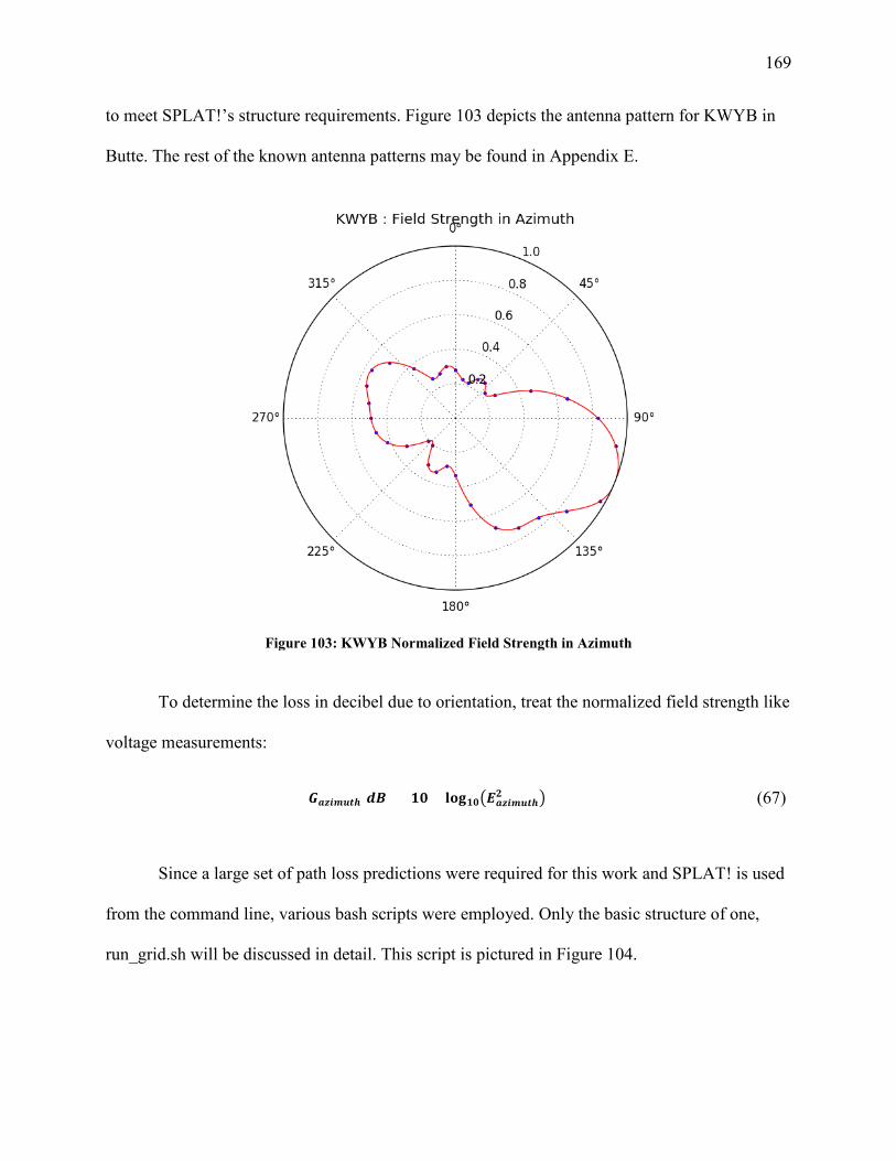
169

to meet SPLAT!’s structure requirements. Figure 103 depicts the antenna pattern for KWYB in

Butte. The rest of the known antenna patterns may be found in Appendix E.

Figure 103: KWYB Normalized Field Strength in Azimuth

To determine the loss in decibel due to orientation, treat the normalized field strength like

voltage measurements:

𝑮𝑮𝒃𝒃𝑯𝑯𝒃𝒃𝒎𝒎𝒎𝒎𝒕𝒕𝒃𝒃[𝒃𝒃𝒅𝒅] = 𝟏𝟏𝟏𝟏 × 𝐥𝐥𝐜𝐜𝐥𝐥𝟏𝟏𝟏𝟏�𝑬𝑬𝒃𝒃𝑯𝑯𝒃𝒃𝒎𝒎𝒎𝒎𝒕𝒕𝒃𝒃𝟐𝟐 � (67)

Since a large set of path loss predictions were required for this work and SPLAT! is used

from the command line, various bash scripts were employed. Only the basic structure of one,

run_grid.sh will be discussed in detail. This script is pictured in Figure 104.

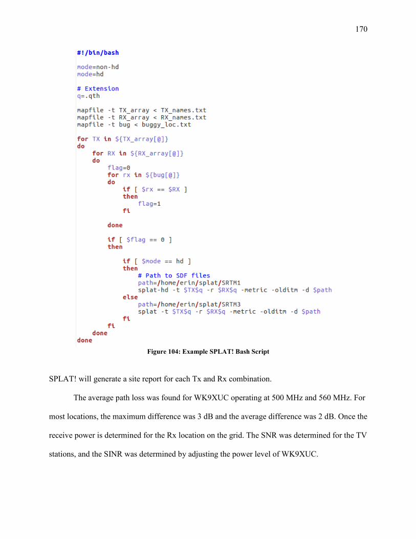
170

Figure 104: Example SPLAT! Bash Script

SPLAT! will generate a site report for each Tx and Rx combination.

The average path loss was found for WK9XUC operating at 500 MHz and 560 MHz. For

most locations, the maximum difference was 3 dB and the average difference was 2 dB. Once the

receive power is determined for the Rx location on the grid. The SNR was determined for the TV

stations, and the SINR was determined by adjusting the power level of WK9XUC.

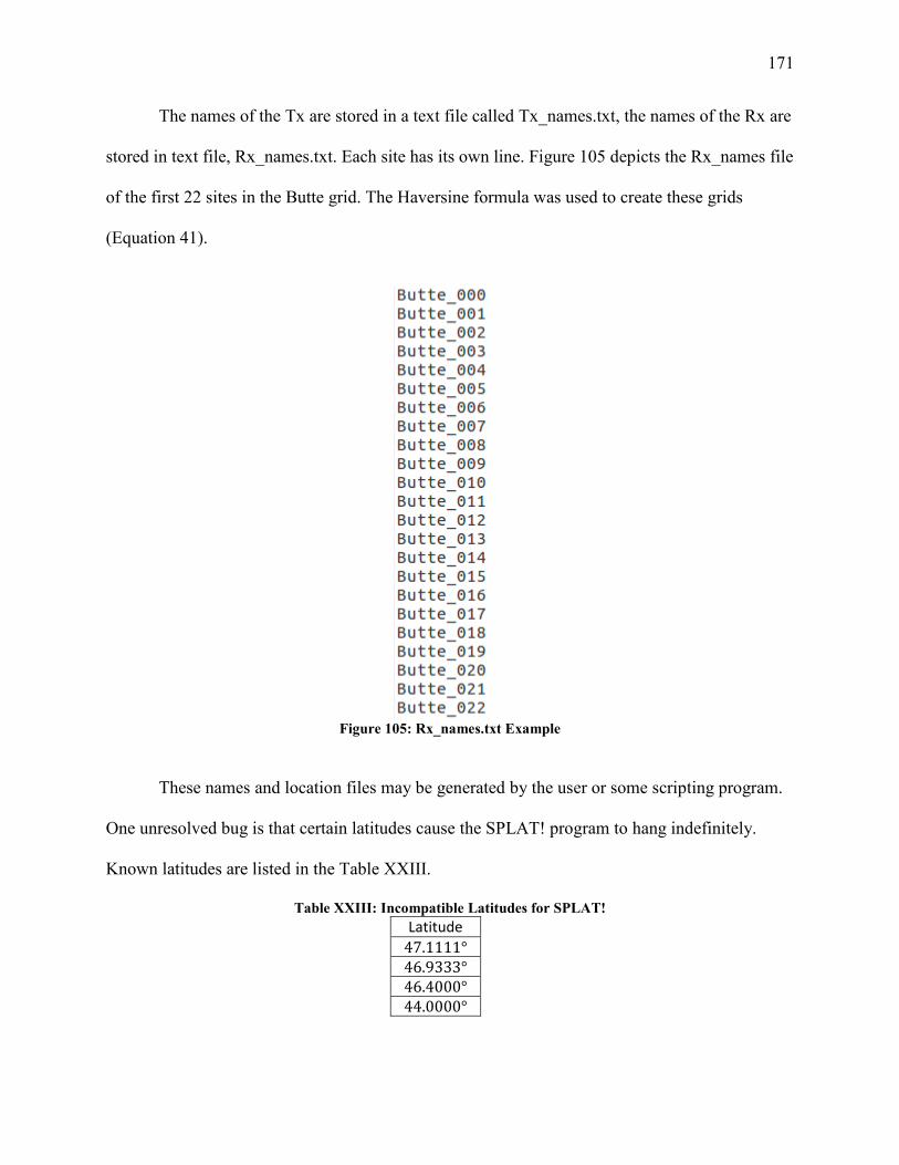
171

The names of the Tx are stored in a text file called Tx_names.txt, the names of the Rx are

stored in text file, Rx_names.txt. Each site has its own line. Figure 105 depicts the Rx_names file

of the first 22 sites in the Butte grid. The Haversine formula was used to create these grids

(Equation 41).

Figure 105: Rx_names.txt Example

These names and location files may be generated by the user or some scripting program.

One unresolved bug is that certain latitudes cause the SPLAT! program to hang indefinitely.

Known latitudes are listed in the Table XXIII.

Table XXIII: Incompatible Latitudes for SPLAT! Latitude

47.1111° 46.9333° 46.4000° 44.0000°

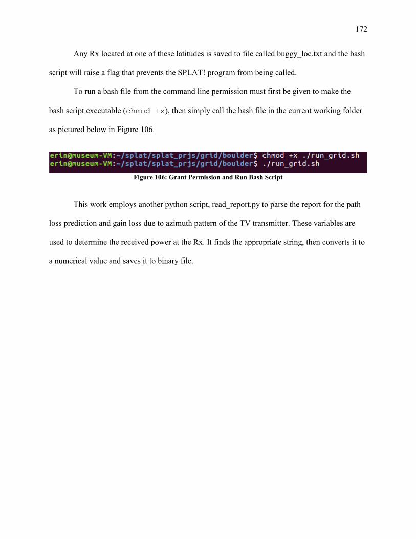
172

Any Rx located at one of these latitudes is saved to file called buggy_loc.txt and the bash

script will raise a flag that prevents the SPLAT! program from being called.

To run a bash file from the command line permission must first be given to make the

bash script executable (chmod +x), then simply call the bash file in the current working folder

as pictured below in Figure 106.

Figure 106: Grant Permission and Run Bash Script

This work employs another python script, read_report.py to parse the report for the path

loss prediction and gain loss due to azimuth pattern of the TV transmitter. These variables are

used to determine the received power at the Rx. It finds the appropriate string, then converts it to

a numerical value and saves it to binary file.

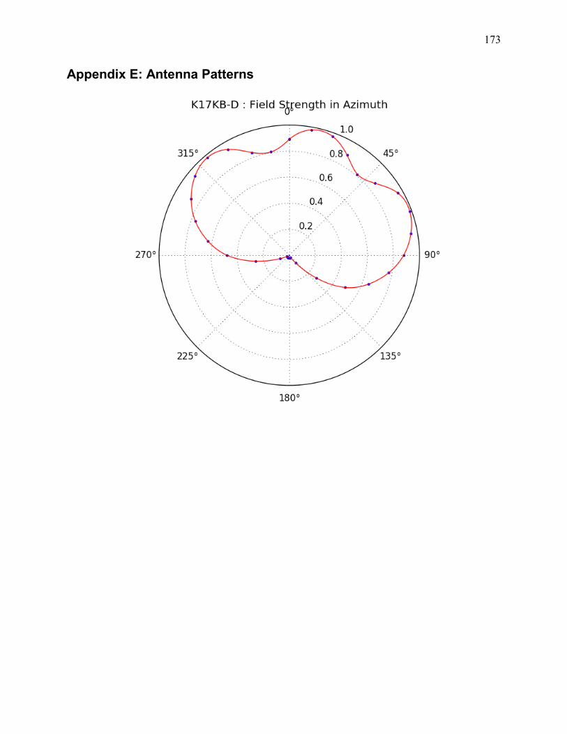
173

Appendix E: Antenna Patterns

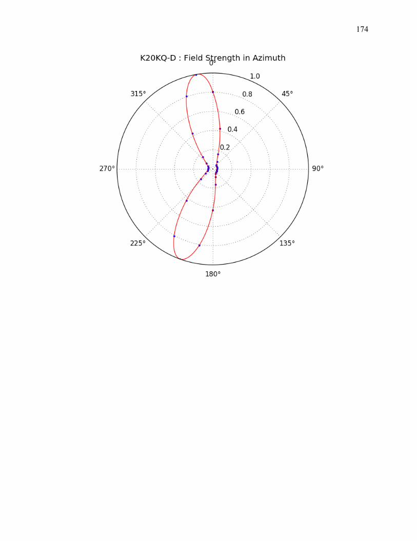
174

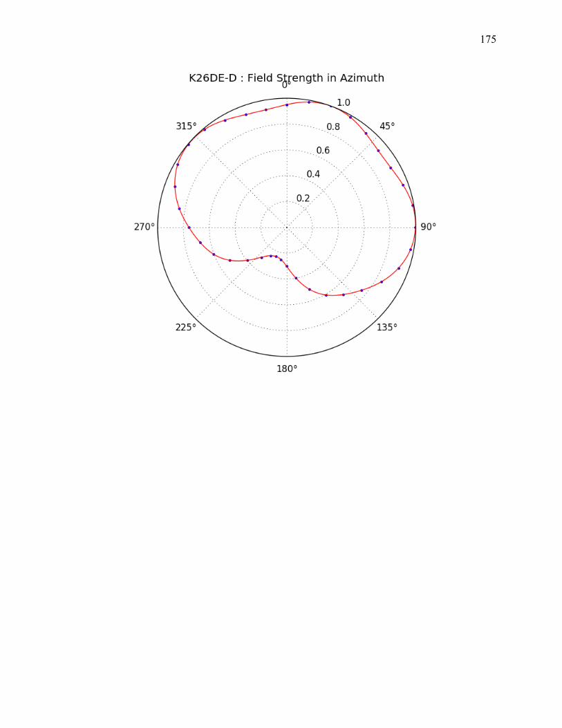
175

176

177

178

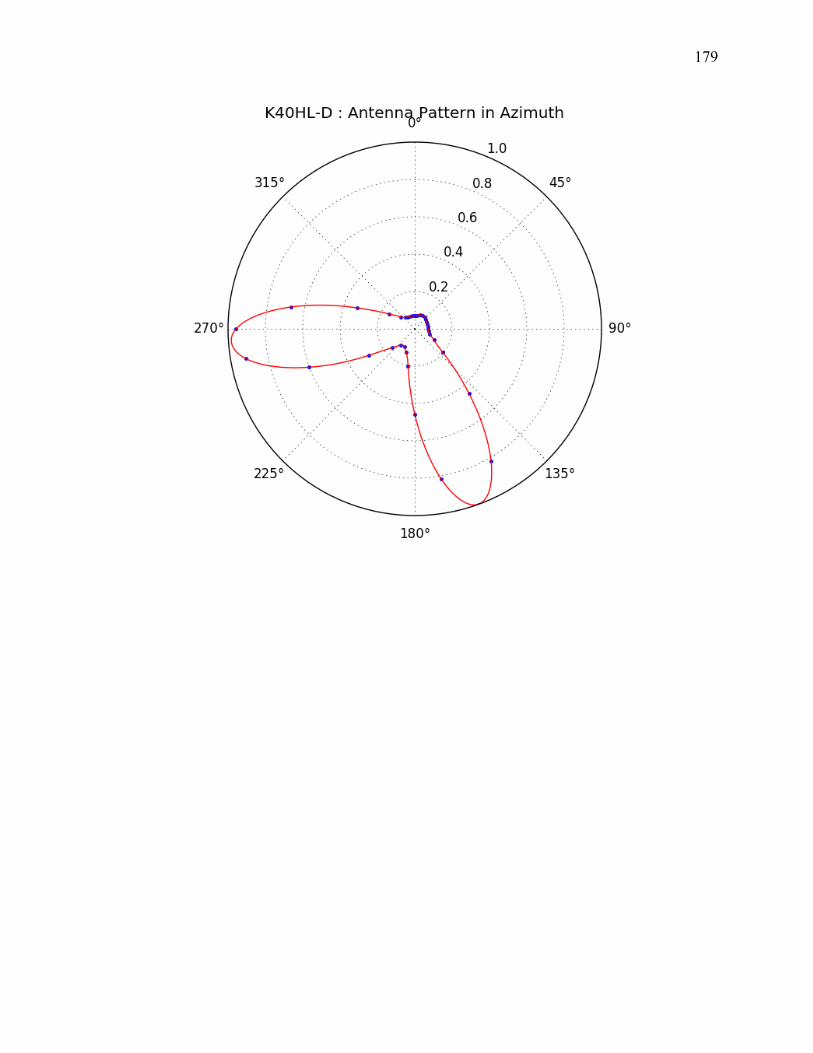
179

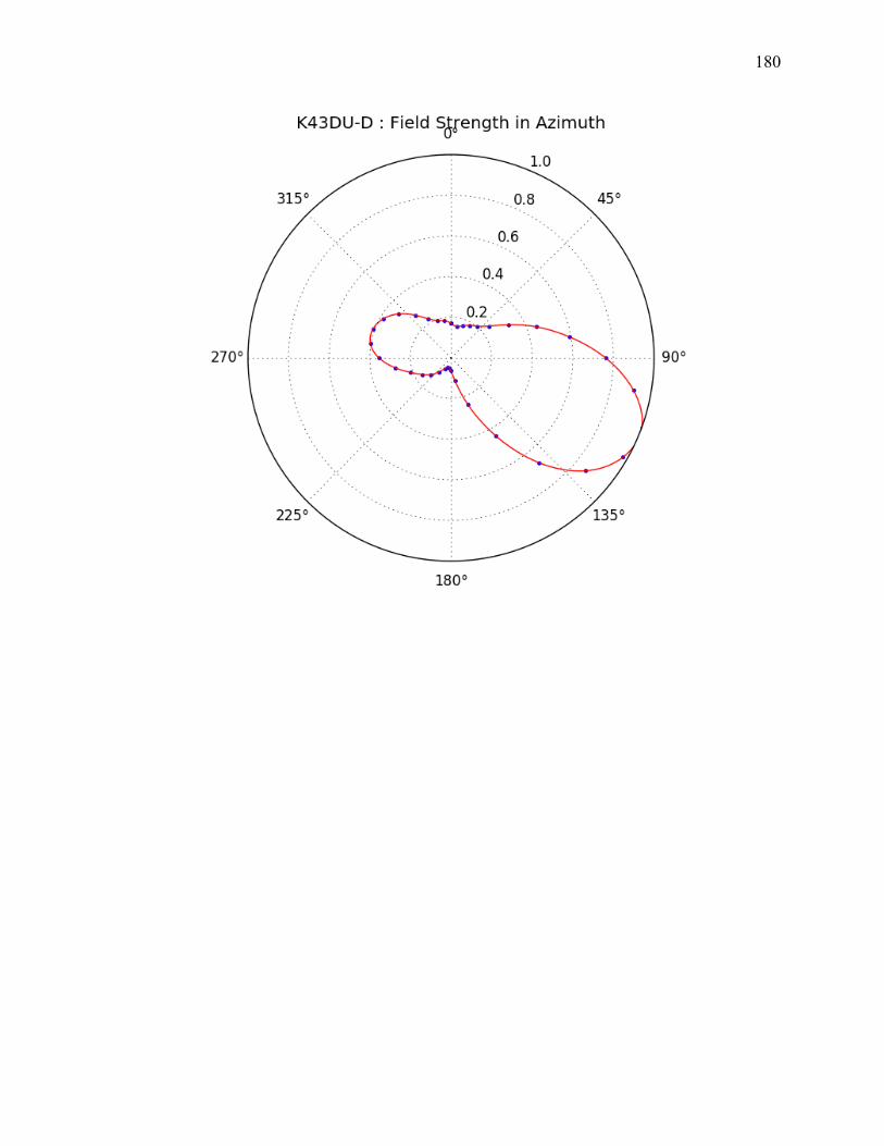
180

181

182

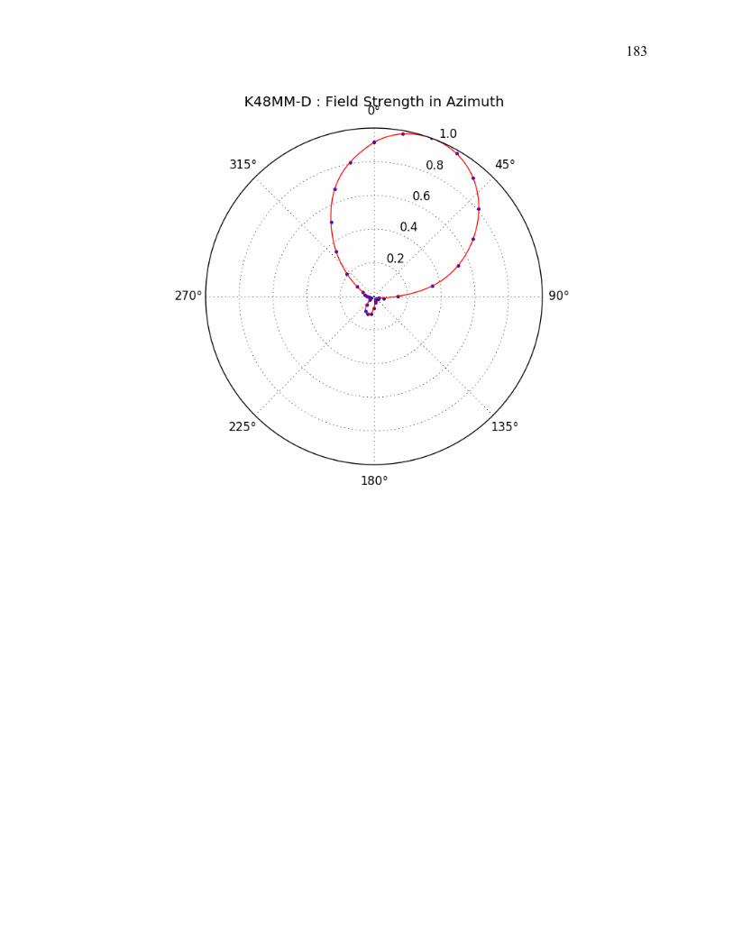
183

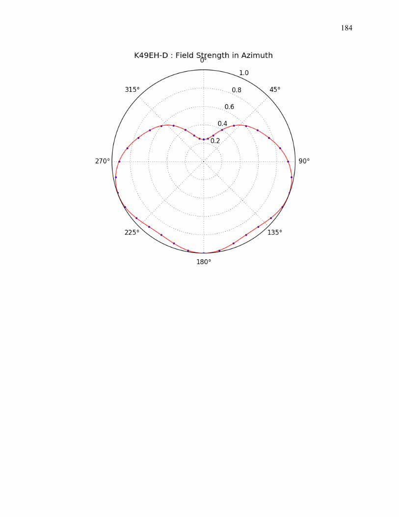
184

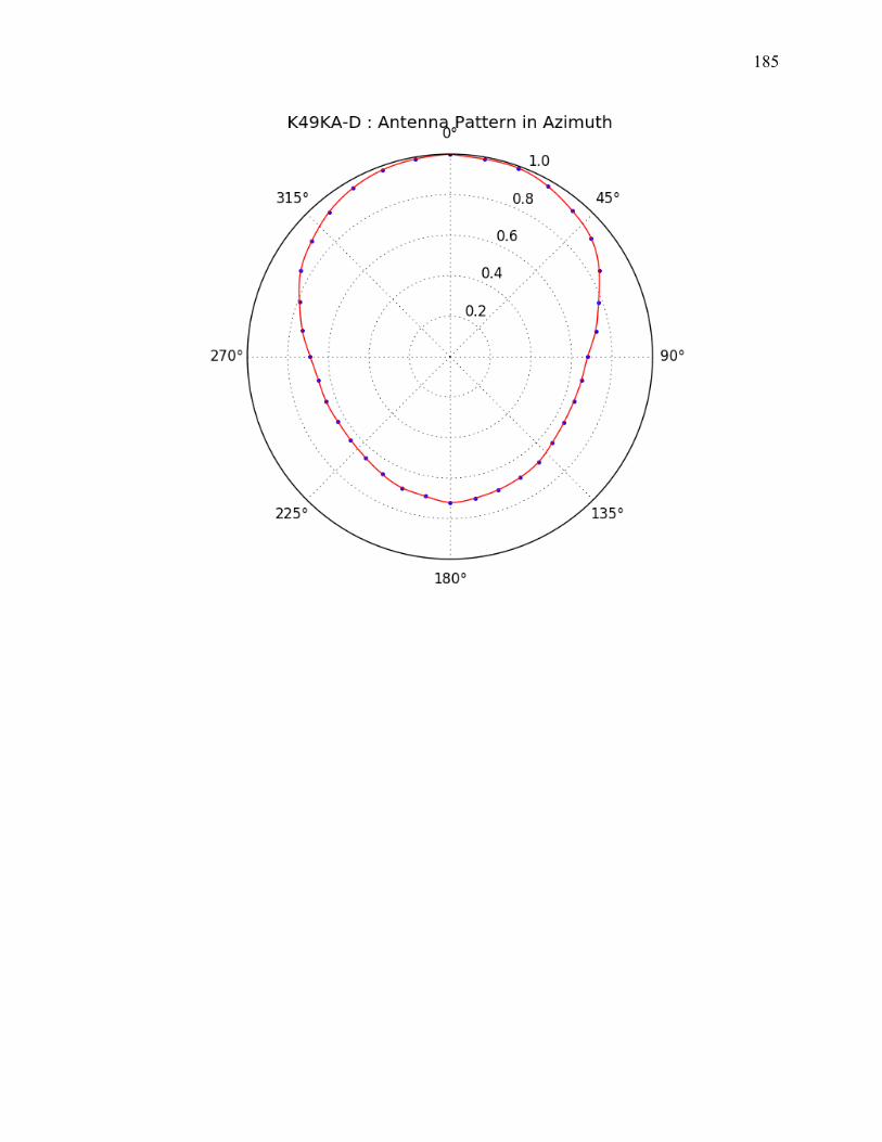
185

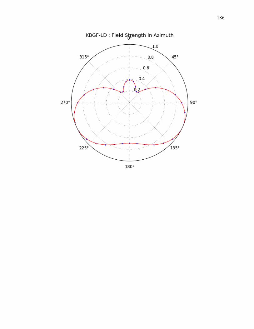
186

187

188

189

190

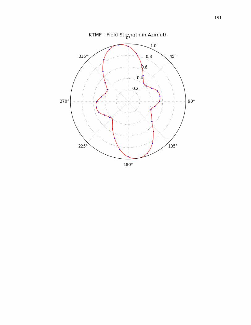
191

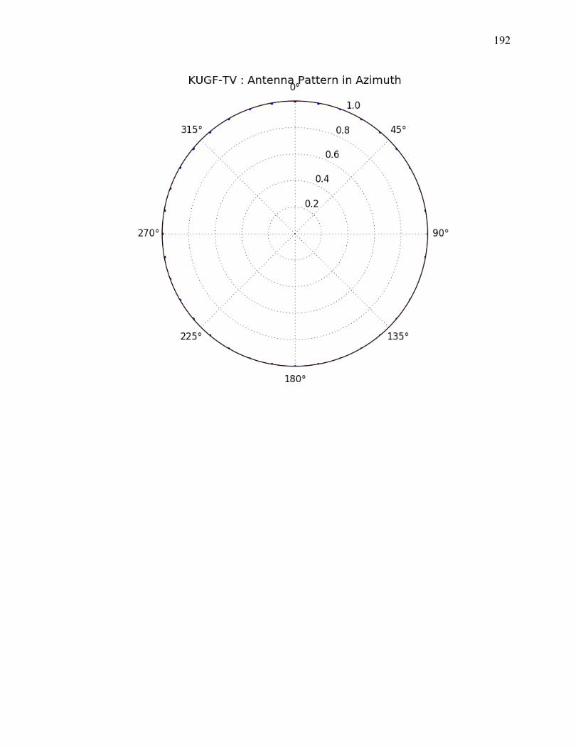
192

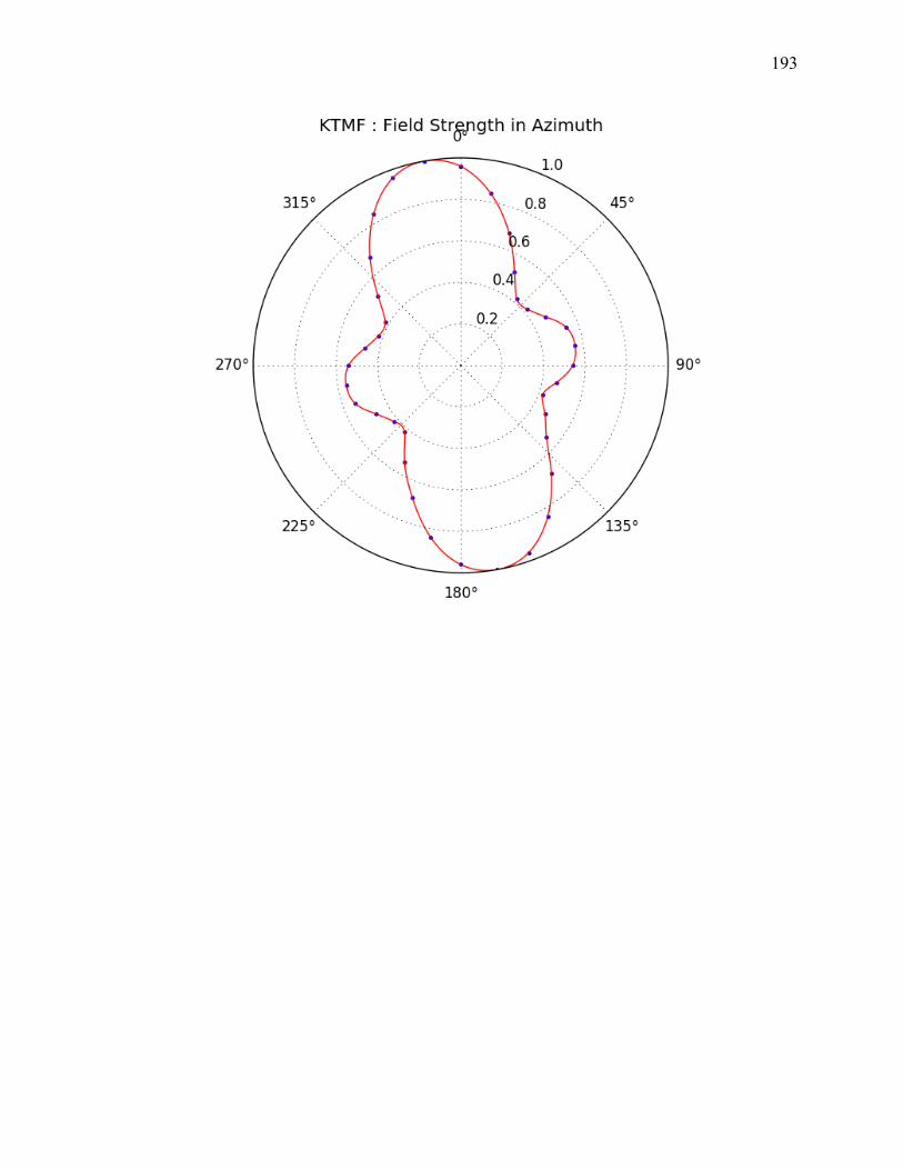
193

194

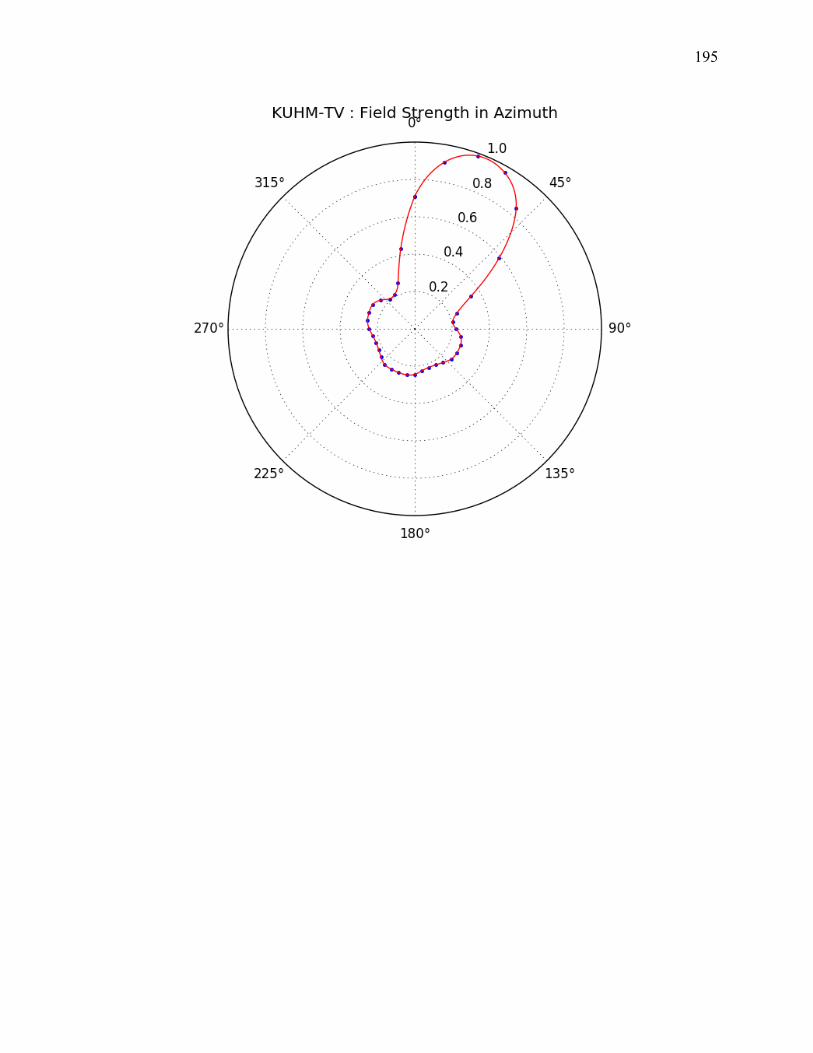
195

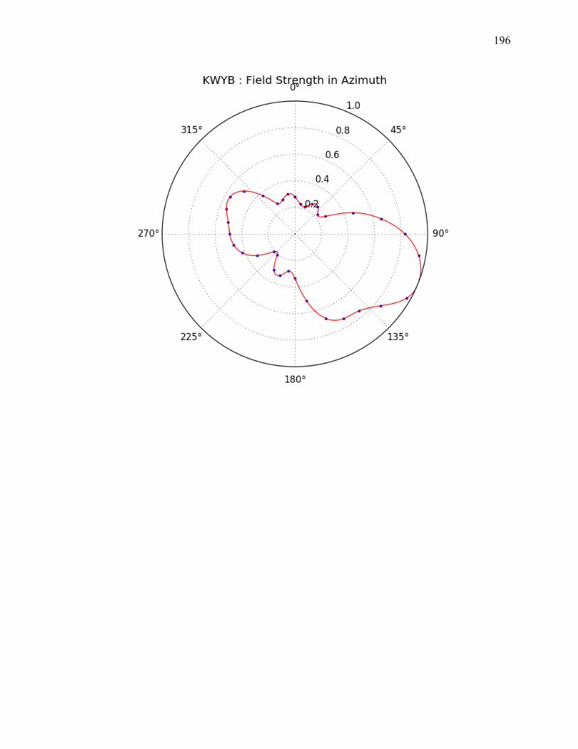
196

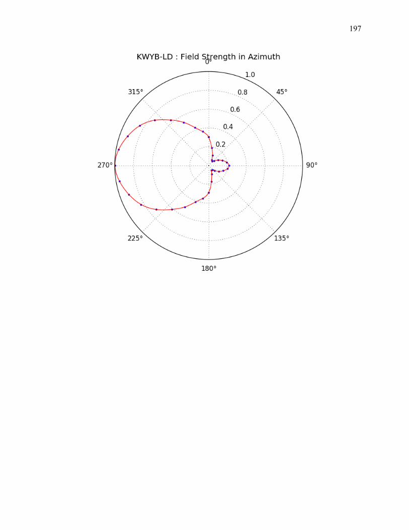
197