Runner Lifting-Up during Load Rejection Transients of ... - MDPI

energies

Article

Runner Lifting-Up during Load Rejection Transientsof a Kaplan Turbine: Flow Mechanism and Solution

Ke Liu 1, Feng Yang 2, Zhiyan Yang 1, Yunxian Zhu 2 and Yongguang Cheng 1,*1 State Key Laboratory of Water Resources and Hydropower Engineering Science, Wuhan University,

Wuhan 430072, China; [email protected] (K.L.); [email protected] (Z.Y.)2 Construction Management Company for Chushandian Reservoir Project of Henan Province,

Zhengzhou 450000, China; [email protected] (F.Y.); [email protected] (Y.Z.)* Correspondence: [email protected]; Tel.: +86-68772274

Received: 18 October 2019; Accepted: 12 December 2019; Published: 15 December 2019�����������������

Abstract: Dangerous runner lifting-up (RLU) accidents regarding Kaplan turbines, which arewidely used in low-head hydropower stations, were frequently reported. Three-dimensional (3D)computational fluid dynamics (CFD) was used to simulate the load rejection transients with guide-vaneclosing to predict the RLU possibility of the fixed-blade Kaplan turbine in an under-constructionhydropower station. It was found that using any linear closing rule, the upward axial water forceon the runner was larger than the weight of rotating parts that started before the guide-vanes wereclosed, which indicated a RLU possibility. It was the pumping effect that caused the imbalance,during which the high rotational speed runner propels water downstream with a low discharge.We proposed a piecewise closing rule based on this finding. By keeping the opening unchanged in aperiod in the closing process, the rotational speed can be reduced by using the braking effect, and theconcurrence of high speed and low discharge can be prevented. Simulations verified this effectivemeasure and accepted by the manufacturer. Although this study used a fixed-blade Kaplan turbine,the revealed mechanism and verified solution to the RLU problem have reference value for all of theKaplan turbines.

Keywords: Kaplan turbine; load rejection transients; runner lifting-up; CFD simulation; flow patterns

1. Introduction

Kaplan turbines are widely used in low-head hydropower stations, because of their highspecific-speed, large discharge capacity, and broad performance zone. The setting-elevations ofKaplan turbines are normally lower due to relative larger cavitation coefficient, which results in largerupward tailwater pressure. During load rejection transient process, which is an emergent shut-downwith rapid closure of guide-vanes due to grid or generator problems, the runner lifting-up (RLU)accident might happen if the upward axial water force is larger than the weight of the rotating parts ofthe turbine-generator unit.

RLU accidents about Kaplan turbines were frequently reported, in which serious damage andproperty losses were accompanied [1–6]. In Kahovskaya Hydroelectric Plant, Russia, a RLU accidenthappened and the runner blades were damaged due to the large rejoining force after water columnseparation during a shut-down transient process [1]. Similar RLU accidents that were caused byreverse water hammer also occurred in Stuguns and Akkats power stations [2], Sweden, in whichwhole shaft lifting and blades breaking were reported. In China, the Kaplan turbines in Hejiatan [3],Mantianxing [4], and Xiacheng [5] hydropower stations encountered several RLU accidents duringload rejection transient processes, which resulted in the destruction of the bearings. Twenty-four RLUs

Energies 2019, 12, 4781; doi:10.3390/en12244781 www.mdpi.com/journal/energies

Energies 2019, 12, 4781 2 of 15

were recorded within the past ten years in Tishrin hydropower station, Syria, causing great damage tothe units [6].

RLUs occur in transient processes, especially the load rejection transient process, during whichfast guide-vane closing can cause large water hammer fluctuations in the draft-tube of Kaplan turbines.Many researches on the load rejection transient process of the Kaplan turbines and RLU reasons havebeen conducted. Chang [7] theoretically analyzed the control mode of Kaplan turbines in transientprocesses and proposed closing guide-vanes in stages and turn blades to the maximum angle beforereaching the maximum speed after load rejection, which has been proven to be reliable and effectiveto improving stability of transient processes by field practice. Cai et al. [8] theoretically analyzedthe RLU reasons of Kaplan turbines, classified the RLU problems into lifting-up by reverse waterhammer and by the pumping effect, and put forward several measures to prevent the RLU problems.Yang et al. [9] reported two RLU problems that are caused by the reverse water hammer and pumpingeffect, respectively, and then analyzed the changing rules of macro-parameters. The reverse waterhammer that caused RLU can be described, as follows: during the load rejection transient process,the rapid closure of guide-vanes causes pressure drop in the draft-tube; the water column can beseparated if the pressure at the runner outlet reaches at the cavitation pressure [10]; the rejoining of theseparated water columns results in an impact on the runner [11]. On the other hand, the pumping effectthat caused RLU can be described, as follows: without reverse water hammer during the load rejectiontransient process, the rotational speed increases while the discharge decreases; the turbine will work ina special mode in which the runner propels water downstream if a high rotational speed encounters alow discharge; if the reaction force of water is large enough the runner can be lifted up. Pejovic [12]gave a formula for predicting water column separation in draft-tube, which considered guide-vaneclosing time, discharge, tailrace tunnel length, and suction head. Yang et al. [9] investigated the RLUprocess of a Kaplan turbine, combining theoretical analysis with engineering tests, and proposed aformula for estimating the lifting force of pumping effect, which is related to the diameter and rotationalspeed of the Kaplan turbine. Min [6] analyzed the causes of RLU of a Kaplan turbine, and solvedthe problem of RLUs while using the methods, which had not been solved in the power station fornearly ten years. The above studies provided many valuable data and measures, however the in-depthanalysis of RLU mechanism of Kaplan turbines is still absent.

Theoretical analysis, engineering tests, and numerical simulations are all useful tools in studyingthe RLUs of Kaplan turbines. Apart from the aforementioned theoretical and simple simulations,engineering tests have achieved good results in practical projects [1–9]. However, prototype testsare not recommended because of being dangerous and consuming many resources. With the rapiddevelopment of computational fluid dynamics (CFD), three-dimensional (3D) CFD simulation becomesa powerful tool to solve turbine flow and unstable problems [13]. Carija et al. [14] and Drtina et al. [15]validated the accuracy of CFD simulations of Kaplan turbines and found that the differences betweenthe simulations and measurements are almost negligible. Liu et al. [16] used CFD to study the steadyoperating conditions of a Kaplan turbine and compared the numerical results with experimental data.Regarding transient process simulations by CFD, Liu et al. [17] simulated the runaway transient processof a Kaplan turbine, Yang et al. [18] simulated the load rejection transient process of a bulb tubularturbine, and Chen et al. [19] simulated the load rejection transient process of a Kaplan turbine whileconsidering the double regulations. These works tell us that 3D CFD is reliable and it can be applied tostudying turbine transient processes.

The RLU phenomenon with a fixed-blade Kaplan turbine during load rejection transient processwas simulated while using the latest 3D CFD in this study to reveal the mechanism of RLUs andfind proper solutions. We attributed the reason of the short-term uprush of axial water force to thedownstream pumping effect by investigating into the varying trends of macro parameters and detailedflow patterns. Based on the mechanism, we proposed and verified a specific designed piecewiseclosing rule to solve the RLU problem. The detailed methods, discussions, and verifications will bepresented in the following sections.

Energies 2019, 12, 4781 3 of 15

2. Numerical Simulation Conditions

2.1. Geometry and Mesh

An under-construction low-head hydropower station with two 1250 kW units and one 400 kWunit was considered. Each unit has its own waterway. One of the 1250 kW units was chosen as thesubject of this study. As shown in Figure 1, the water system includes an upper reservoir (waterlevel 88.00 m), a penstock (length 35.0 m, average diameter 2.5 m), a fixed-blade Kaplan turbine unit(rated-head 11.13 m, rated discharge 13.8 m3/s), a tailrace tunnel (length 10.6 m, average cross-section9.6 m2), and downstream (water level 74.91 m). Table 1 lists the detailed specifications of the Kaplanturbine, where D1 is the diameter of the runner, nr is the rated rotational speed, W is the total weight ofrotating parts (including the Kaplan turbine and generator rotor), Wa is the wrap angle of spiral-casing,zb, nsv, and ngv are the numbers of runner blades, stay-vanes, and guide-vanes, respectively. In thisstudy, the starting operation point that is shown in Figure 2 with a red square point is the rated point;all of the parameters are the same as the rated parameters.

Energies 2019, 10, x FOR PEER REVIEW 3 of 15

2. Numerical Simulation Conditions

2.1. Geometry and Mesh

An under-construction low-head hydropower station with two 1250 kW units and one 400 kW unit was considered. Each unit has its own waterway. One of the 1250 kW units was chosen as the subject of this study. As shown in Figure 1, the water system includes an upper reservoir (water level 88.00 m), a penstock (length 35.0 m, average diameter 2.5 m), a fixed-blade Kaplan turbine unit (rated-head 11.13 m, rated discharge 13.8 m3/s), a tailrace tunnel (length 10.6 m, average cross-section 9.6 m2), and downstream (water level 74.91 m). Table 1 lists the detailed specifications of the Kaplan turbine, where D1 is the diameter of the runner, nr is the rated rotational speed, W is the total weight of rotating parts (including the Kaplan turbine and generator rotor), Wa is the wrap angle of spiral-casing, zb, nsv, and ngv are the numbers of runner blades, stay-vanes, and guide-vanes, respectively. In this study, the starting operation point that is shown in Figure 2 with a red square point is the rated point; all of the parameters are the same as the rated parameters.

Figure 1. Three-dimensional (3D) computational domains of the waterway and Kaplan turbine unit.

Table 1. Parameters of the Kaplan turbine.

D1 (m) nr (rpm) W (kN) Wa (deg) zb nsv ngv 1.6 250 140 180 5 14 14

1100 1300 1500 1700 1900 210075

95

115

135

155

175

84

8082

78

86

88

89

90n 11(r

/min

)

Q11(l/s)

46º

26º28º

44º

30º

42º40º

38º36º

32º34º

a=28°a=32°a=36°a=40°a=44°

Starting operation point

Figure 2. Comparisons between the simulated results and measured characteristic curves. n11 = n ∙ D1 / √H; Q11 = Q / (D1

2 ∙ √H).

Hybrid mesh was generated while using software ANSYS ICEM 17.0 (ANSYS, Canonsburg, PA, USA) in different domains: wedge mesh in guide-vanes domain and hexahedral mesh in the rest domains (upper reservoir, penstock, spiral-casing, stay-vanes, vaneless space, runner, draft-tube, tailrace tunnel, and downstream). The hexahedral grids at the leading and trailing edge of the runner are locally refined, as shown in Figure 3.

Figure 1. Three-dimensional (3D) computational domains of the waterway and Kaplan turbine unit.

Table 1. Parameters of the Kaplan turbine.

D1 (m) nr (rpm) W (kN) Wa (deg) zb nsv ngv

1.6 250 140 180 5 14 14

Energies 2019, 10, x FOR PEER REVIEW 3 of 15

2. Numerical Simulation Conditions

2.1. Geometry and Mesh

An under-construction low-head hydropower station with two 1250 kW units and one 400 kW unit was considered. Each unit has its own waterway. One of the 1250 kW units was chosen as the subject of this study. As shown in Figure 1, the water system includes an upper reservoir (water level 88.00 m), a penstock (length 35.0 m, average diameter 2.5 m), a fixed-blade Kaplan turbine unit (rated-head 11.13 m, rated discharge 13.8 m3/s), a tailrace tunnel (length 10.6 m, average cross-section 9.6 m2), and downstream (water level 74.91 m). Table 1 lists the detailed specifications of the Kaplan turbine, where D1 is the diameter of the runner, nr is the rated rotational speed, W is the total weight of rotating parts (including the Kaplan turbine and generator rotor), Wa is the wrap angle of spiral-casing, zb, nsv, and ngv are the numbers of runner blades, stay-vanes, and guide-vanes, respectively. In this study, the starting operation point that is shown in Figure 2 with a red square point is the rated point; all of the parameters are the same as the rated parameters.

Figure 1. Three-dimensional (3D) computational domains of the waterway and Kaplan turbine unit.

Table 1. Parameters of the Kaplan turbine.

D1 (m) nr (rpm) W (kN) Wa (deg) zb nsv ngv 1.6 250 140 180 5 14 14

1100 1300 1500 1700 1900 210075

95

115

135

155

175

84

8082

78

86

88

89

90n 11(r

/min

)

Q11(l/s)

46º

26º28º

44º

30º

42º40º

38º36º

32º34º

a=28°a=32°a=36°a=40°a=44°

Starting operation point

Figure 2. Comparisons between the simulated results and measured characteristic curves. n11 = n ∙ D1 / √H; Q11 = Q / (D1

2 ∙ √H).

Hybrid mesh was generated while using software ANSYS ICEM 17.0 (ANSYS, Canonsburg, PA, USA) in different domains: wedge mesh in guide-vanes domain and hexahedral mesh in the rest domains (upper reservoir, penstock, spiral-casing, stay-vanes, vaneless space, runner, draft-tube, tailrace tunnel, and downstream). The hexahedral grids at the leading and trailing edge of the runner are locally refined, as shown in Figure 3.

Figure 2. Comparisons between the simulated results and measured characteristic curves.n11= n·D1/

√H; Q11= Q/(D 2

1·√

H).

Hybrid mesh was generated while using software ANSYS ICEM 17.0 (ANSYS, Canonsburg,PA, USA) in different domains: wedge mesh in guide-vanes domain and hexahedral mesh in therest domains (upper reservoir, penstock, spiral-casing, stay-vanes, vaneless space, runner, draft-tube,tailrace tunnel, and downstream). The hexahedral grids at the leading and trailing edge of the runnerare locally refined, as shown in Figure 3.

Energies 2019, 12, 4781 4 of 15Energies 2019, 10, x FOR PEER REVIEW 4 of 15

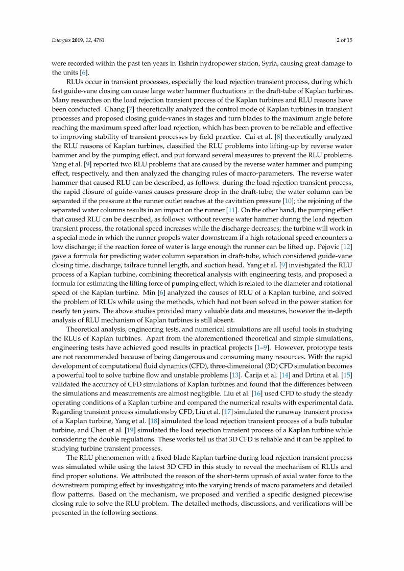
Figure 3. Hexahedral grids around the runner.

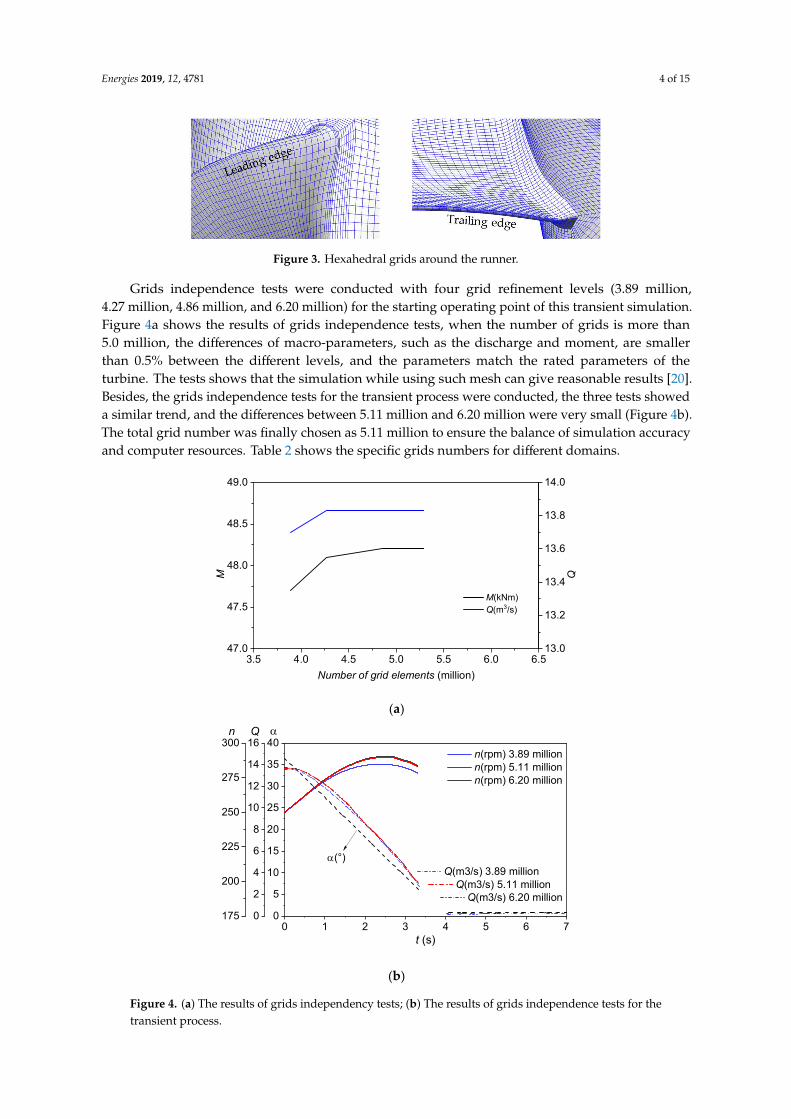
Grids independence tests were conducted with four grid refinement levels (3.89 million, 4.27 million, 4.86 million, and 6.20 million) for the starting operating point of this transient simulation. Figure 4a shows the results of grids independence tests, when the number of grids is more than 5.0 million, the differences of macro-parameters, such as the discharge and moment, are smaller than 0.5% between the different levels, and the parameters match the rated parameters of the turbine. The tests shows that the simulation while using such mesh can give reasonable results [20]. Besides, the grids independence tests for the transient process were conducted, the three tests showed a similar trend, and the differences between 5.11 million and 6.20 million were very small (Figure 4b). The total grid number was finally chosen as 5.11 million to ensure the balance of simulation accuracy and computer resources. Table 2 shows the specific grids numbers for different domains.

3.5 4.0 4.5 5.0 5.5 6.0 6.547.0

47.5

48.0

48.5

49.0

M(kNm)Q(m3/s)

M

Number of grid elements (million)

13.0

13.2

13.4

13.6

13.8

14.0

Q

(a)

0 1 2 3 4 5 6 70

5

10

15

20

25

30

35

40

a(°)Q(m3/s) 3.89 million

Q(m3/s) 5.11 million Q(m3/s) 6.20 million

n(rpm) 3.89 millionn(rpm) 5.11 millionn(rpm) 6.20 million

t (s)

aQn

175

200

225

250

275

300

0

2

4

6

8

10

12

14

16

(b)

Figure 4. The results of grids independency tests.

Figure 3. Hexahedral grids around the runner.

Grids independence tests were conducted with four grid refinement levels (3.89 million,4.27 million, 4.86 million, and 6.20 million) for the starting operating point of this transient simulation.Figure 4a shows the results of grids independence tests, when the number of grids is more than5.0 million, the differences of macro-parameters, such as the discharge and moment, are smallerthan 0.5% between the different levels, and the parameters match the rated parameters of theturbine. The tests shows that the simulation while using such mesh can give reasonable results [20].Besides, the grids independence tests for the transient process were conducted, the three tests showeda similar trend, and the differences between 5.11 million and 6.20 million were very small (Figure 4b).The total grid number was finally chosen as 5.11 million to ensure the balance of simulation accuracyand computer resources. Table 2 shows the specific grids numbers for different domains.

Energies 2019, 10, x FOR PEER REVIEW 4 of 15

Figure 3. Hexahedral grids around the runner.

Grids independence tests were conducted with four grid refinement levels (3.89 million, 4.27 million, 4.86 million, and 6.20 million) for the starting operating point of this transient simulation. Figure 4a shows the results of grids independence tests, when the number of grids is more than 5.0 million, the differences of macro-parameters, such as the discharge and moment, are smaller than 0.5% between the different levels, and the parameters match the rated parameters of the turbine. The tests shows that the simulation while using such mesh can give reasonable results [20]. Besides, the grids independence tests for the transient process were conducted, the three tests showed a similar trend, and the differences between 5.11 million and 6.20 million were very small (Figure 4b). The total grid number was finally chosen as 5.11 million to ensure the balance of simulation accuracy and computer resources. Table 2 shows the specific grids numbers for different domains.

3.5 4.0 4.5 5.0 5.5 6.0 6.547.0

47.5

48.0

48.5

49.0

M(kNm)Q(m3/s)

M

Number of grid elements (million)

13.0

13.2

13.4

13.6

13.8

14.0

Q

(a)

0 1 2 3 4 5 6 70

5

10

15

20

25

30

35

40

a(°)Q(m3/s) 3.89 million

Q(m3/s) 5.11 million Q(m3/s) 6.20 million

n(rpm) 3.89 millionn(rpm) 5.11 millionn(rpm) 6.20 million

t (s)

aQn

175

200

225

250

275

300

0

2

4

6

8

10

12

14

16

(b)

Figure 4. The results of grids independency tests. Figure 4. (a) The results of grids independency tests; (b) The results of grids independence tests for thetransient process.

Energies 2019, 12, 4781 5 of 15

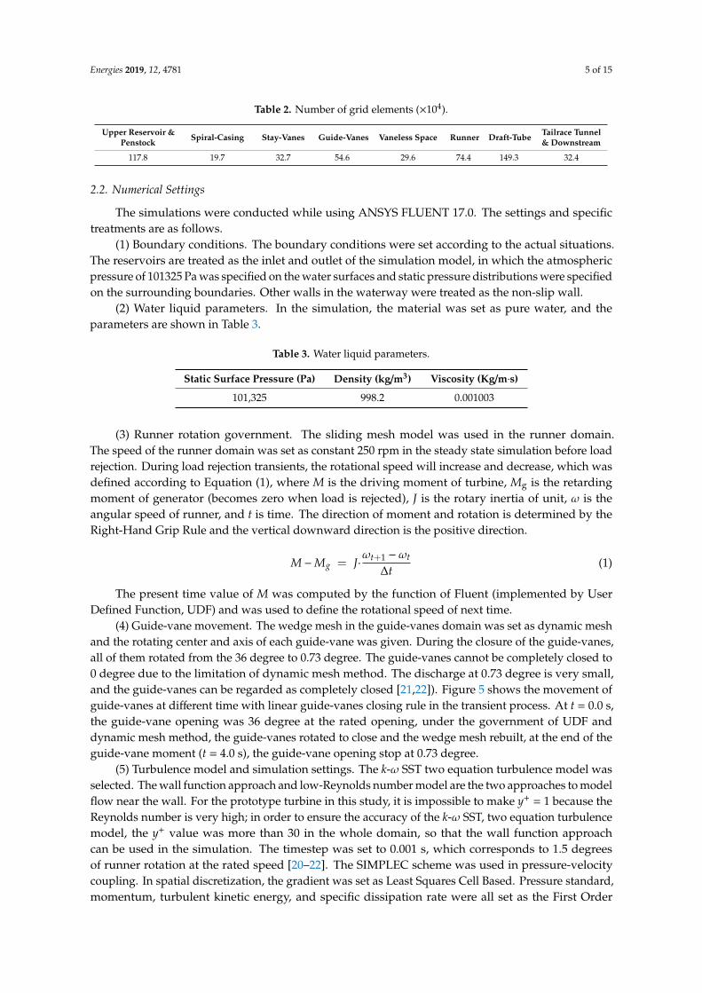
Table 2. Number of grid elements (×104).

Upper Reservoir &Penstock Spiral-Casing Stay-Vanes Guide-Vanes Vaneless Space Runner Draft-Tube Tailrace Tunnel

& Downstream

117.8 19.7 32.7 54.6 29.6 74.4 149.3 32.4

2.2. Numerical Settings

The simulations were conducted while using ANSYS FLUENT 17.0. The settings and specifictreatments are as follows.

(1) Boundary conditions. The boundary conditions were set according to the actual situations.The reservoirs are treated as the inlet and outlet of the simulation model, in which the atmosphericpressure of 101325 Pa was specified on the water surfaces and static pressure distributions were specifiedon the surrounding boundaries. Other walls in the waterway were treated as the non-slip wall.

(2) Water liquid parameters. In the simulation, the material was set as pure water, and theparameters are shown in Table 3.

Table 3. Water liquid parameters.

Static Surface Pressure (Pa) Density (kg/m3) Viscosity (Kg/m·s)

101,325 998.2 0.001003

(3) Runner rotation government. The sliding mesh model was used in the runner domain.The speed of the runner domain was set as constant 250 rpm in the steady state simulation before loadrejection. During load rejection transients, the rotational speed will increase and decrease, which wasdefined according to Equation (1), where M is the driving moment of turbine, Mg is the retardingmoment of generator (becomes zero when load is rejected), J is the rotary inertia of unit, ω is theangular speed of runner, and t is time. The direction of moment and rotation is determined by theRight-Hand Grip Rule and the vertical downward direction is the positive direction.

M−Mg = J·ωt+1 −ωt

∆t(1)

The present time value of M was computed by the function of Fluent (implemented by UserDefined Function, UDF) and was used to define the rotational speed of next time.

(4) Guide-vane movement. The wedge mesh in the guide-vanes domain was set as dynamic meshand the rotating center and axis of each guide-vane was given. During the closure of the guide-vanes,all of them rotated from the 36 degree to 0.73 degree. The guide-vanes cannot be completely closed to0 degree due to the limitation of dynamic mesh method. The discharge at 0.73 degree is very small,and the guide-vanes can be regarded as completely closed [21,22]). Figure 5 shows the movement ofguide-vanes at different time with linear guide-vanes closing rule in the transient process. At t = 0.0 s,the guide-vane opening was 36 degree at the rated opening, under the government of UDF anddynamic mesh method, the guide-vanes rotated to close and the wedge mesh rebuilt, at the end of theguide-vane moment (t = 4.0 s), the guide-vane opening stop at 0.73 degree.

(5) Turbulence model and simulation settings. The k-ω SST two equation turbulence model wasselected. The wall function approach and low-Reynolds number model are the two approaches to modelflow near the wall. For the prototype turbine in this study, it is impossible to make y+ = 1 because theReynolds number is very high; in order to ensure the accuracy of the k-ω SST, two equation turbulencemodel, the y+ value was more than 30 in the whole domain, so that the wall function approachcan be used in the simulation. The timestep was set to 0.001 s, which corresponds to 1.5 degreesof runner rotation at the rated speed [20–22]. The SIMPLEC scheme was used in pressure-velocitycoupling. In spatial discretization, the gradient was set as Least Squares Cell Based. Pressure standard,momentum, turbulent kinetic energy, and specific dissipation rate were all set as the First Order

Energies 2019, 12, 4781 6 of 15

Upwind. In the transient simulation, the residuals of continuity, velocities, k and ω at each timestepwere 1 × 10−5, and the maximum iteration number of each timestep was set to 50.Energies 2019, 10, x FOR PEER REVIEW 6 of 15

Figure 5. Movement of guide-vanes with dynamic mesh method.

(5) Turbulence model and simulation settings. The k-ω SST two equation turbulence model was selected. The wall function approach and low-Reynolds number model are the two approaches to model flow near the wall. For the prototype turbine in this study, it is impossible to make y+ = 1 because the Reynolds number is very high; in order to ensure the accuracy of the k-ω SST, two equation turbulence model, the y+ value was more than 30 in the whole domain, so that the wall function approach can be used in the simulation. The timestep was set to 0.001 s, which corresponds to 1.5 degrees of runner rotation at the rated speed [20–22]. The SIMPLEC scheme was used in pressure-velocity coupling. In spatial discretization, the gradient was set as Least Squares Cell Based. Pressure standard, momentum, turbulent kinetic energy, and specific dissipation rate were all set as the First Order Upwind. In the transient simulation, the residuals of continuity, velocities, k and ω at each timestep were 1 × 10−5, and the maximum iteration number of each timestep was set to 50.

2.3. Accuracy Validation

We used the CFD model to simulate 23 static operating points at five different openings and compared them with the characteristic curves measured in model tests of the manufacturer to validate the reliability of the simulation. Figure 2 shows the comparison, in which Q11 and n11 are the unit discharge and unit speed, respectively. We found that the results of the simulated points agree with the measured curves quite well, with the relative error near the rated operating point being smaller than 2%. The relative errors for the operating regions far from the rated operating point become larger, but the largest one is smaller than 5%.

2.4. Layout of Monitoring Points

The monitoring points (P1, P2) were arranged ahead and behind the guide-vanes in the middle span of guide-vane domain to detect the pressure fluctuation histories during the guide-vane closing process, as shown in Figure 6. Monitoring points P3, P4, P5, and P6 were also set to monitor the pressure fluctuations around the runner and to supervise the occurrence of water column separation.

Figure 6. Layout of monitoring points.

Figure 5. Movement of guide-vanes with dynamic mesh method.

2.3. Accuracy Validation

We used the CFD model to simulate 23 static operating points at five different openings andcompared them with the characteristic curves measured in model tests of the manufacturer to validatethe reliability of the simulation. Figure 2 shows the comparison, in which Q11 and n11 are the unitdischarge and unit speed, respectively. We found that the results of the simulated points agree withthe measured curves quite well, with the relative error near the rated operating point being smallerthan 2%. The relative errors for the operating regions far from the rated operating point become larger,but the largest one is smaller than 5%.

2.4. Layout of Monitoring Points

The monitoring points (P1, P2) were arranged ahead and behind the guide-vanes in the middlespan of guide-vane domain to detect the pressure fluctuation histories during the guide-vane closingprocess, as shown in Figure 6. Monitoring points P3, P4, P5, and P6 were also set to monitor thepressure fluctuations around the runner and to supervise the occurrence of water column separation.

Energies 2019, 10, x FOR PEER REVIEW 6 of 15

Figure 5. Movement of guide-vanes with dynamic mesh method.

(5) Turbulence model and simulation settings. The k-ω SST two equation turbulence model was selected. The wall function approach and low-Reynolds number model are the two approaches to model flow near the wall. For the prototype turbine in this study, it is impossible to make y+ = 1 because the Reynolds number is very high; in order to ensure the accuracy of the k-ω SST, two equation turbulence model, the y+ value was more than 30 in the whole domain, so that the wall function approach can be used in the simulation. The timestep was set to 0.001 s, which corresponds to 1.5 degrees of runner rotation at the rated speed [20–22]. The SIMPLEC scheme was used in pressure-velocity coupling. In spatial discretization, the gradient was set as Least Squares Cell Based. Pressure standard, momentum, turbulent kinetic energy, and specific dissipation rate were all set as the First Order Upwind. In the transient simulation, the residuals of continuity, velocities, k and ω at each timestep were 1 × 10−5, and the maximum iteration number of each timestep was set to 50.

2.3. Accuracy Validation

We used the CFD model to simulate 23 static operating points at five different openings and compared them with the characteristic curves measured in model tests of the manufacturer to validate the reliability of the simulation. Figure 2 shows the comparison, in which Q11 and n11 are the unit discharge and unit speed, respectively. We found that the results of the simulated points agree with the measured curves quite well, with the relative error near the rated operating point being smaller than 2%. The relative errors for the operating regions far from the rated operating point become larger, but the largest one is smaller than 5%.

2.4. Layout of Monitoring Points

The monitoring points (P1, P2) were arranged ahead and behind the guide-vanes in the middle span of guide-vane domain to detect the pressure fluctuation histories during the guide-vane closing process, as shown in Figure 6. Monitoring points P3, P4, P5, and P6 were also set to monitor the pressure fluctuations around the runner and to supervise the occurrence of water column separation.

Figure 6. Layout of monitoring points. Figure 6. Layout of monitoring points.

3. Load Rejection Transients with Linear Guide-Vanes Closing Rule

When load rejection is detected, the governor will drive the guide-vanes to close following a givenrule. During the closing process, water hammer waves will be generated due to discharge decrease,with positive value ahead of the guide-vanes and the negative value behind them. The rotationalspeed will increase first due to the absence of the resistance moment Mg, and then decrease dueto the decrease and sign reversing of the driving moment M from negative to positive, as inEquation (1). The phenomena composed of load rejection action, guide-vane closure, discharge

Energies 2019, 12, 4781 7 of 15

decrease, water hammer generation, transmission and reflection, and speed increase and decrease,are generally called the load rejection transients.

We first simulated the load rejection transients with a linear guide-vane closing rule in this study.

3.1. Variations of Macro Parameters

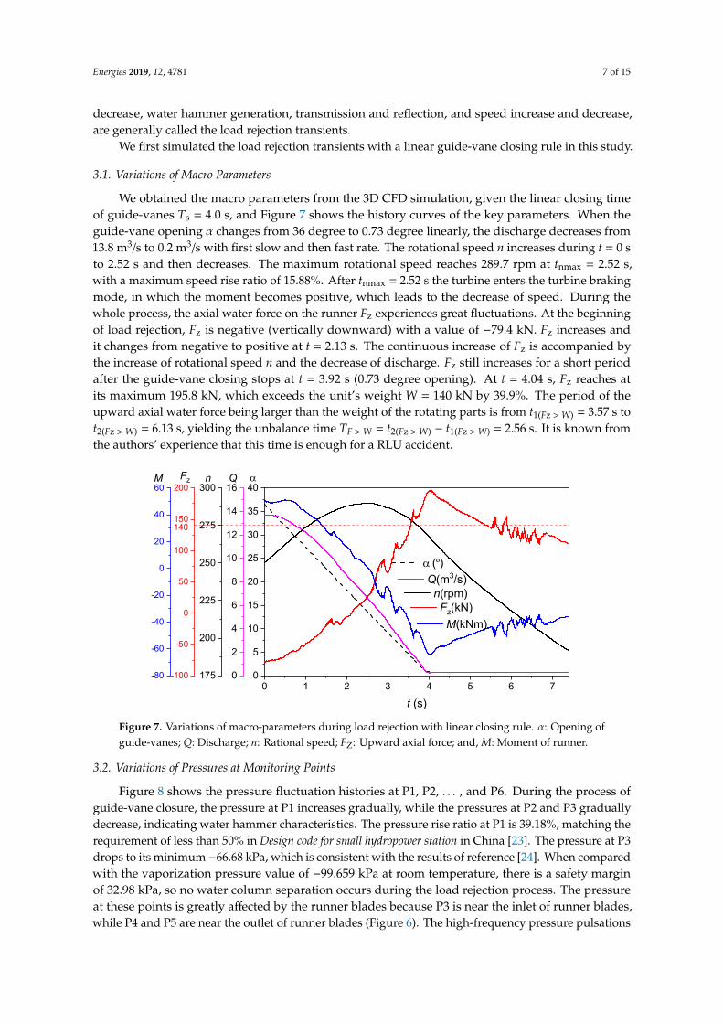
We obtained the macro parameters from the 3D CFD simulation, given the linear closing timeof guide-vanes Ts = 4.0 s, and Figure 7 shows the history curves of the key parameters. When theguide-vane opening α changes from 36 degree to 0.73 degree linearly, the discharge decreases from13.8 m3/s to 0.2 m3/s with first slow and then fast rate. The rotational speed n increases during t = 0 sto 2.52 s and then decreases. The maximum rotational speed reaches 289.7 rpm at tnmax = 2.52 s,with a maximum speed rise ratio of 15.88%. After tnmax = 2.52 s the turbine enters the turbine brakingmode, in which the moment becomes positive, which leads to the decrease of speed. During thewhole process, the axial water force on the runner Fz experiences great fluctuations. At the beginningof load rejection, Fz is negative (vertically downward) with a value of −79.4 kN. Fz increases andit changes from negative to positive at t = 2.13 s. The continuous increase of Fz is accompanied bythe increase of rotational speed n and the decrease of discharge. Fz still increases for a short periodafter the guide-vane closing stops at t = 3.92 s (0.73 degree opening). At t = 4.04 s, Fz reaches atits maximum 195.8 kN, which exceeds the unit’s weight W = 140 kN by 39.9%. The period of theupward axial water force being larger than the weight of the rotating parts is from t1(Fz > W) = 3.57 s tot2(Fz > W) = 6.13 s, yielding the unbalance time TF > W = t2(Fz > W) − t1(Fz > W) = 2.56 s. It is known fromthe authors’ experience that this time is enough for a RLU accident.

Energies 2019, 10, x FOR PEER REVIEW 7 of 15

3. Load Rejection Transients with Linear Guide-Vanes Closing Rule

When load rejection is detected, the governor will drive the guide-vanes to close following a given rule. During the closing process, water hammer waves will be generated due to discharge decrease, with positive value ahead of the guide-vanes and the negative value behind them. The rotational speed will increase first due to the absence of the resistance moment Mg, and then decrease due to the decrease and sign reversing of the driving moment M from negative to positive, as in Equation (1). The phenomena composed of load rejection action, guide-vane closure, discharge decrease, water hammer generation, transmission and reflection, and speed increase and decrease, are generally called the load rejection transients.

We first simulated the load rejection transients with a linear guide-vane closing rule in this study.

3.1. Variations of Macro Parameters

We obtained the macro parameters from the 3D CFD simulation, given the linear closing time of guide-vanes Ts = 4.0 s, and Figure 7 shows the history curves of the key parameters. When the guide-vane opening α changes from 36 degree to 0.73 degree linearly, the discharge decreases from 13.8 m3/s to 0.2 m3/s with first slow and then fast rate. The rotational speed n increases during t = 0 s to 2.52 s and then decreases. The maximum rotational speed reaches 289.7 rpm at tnmax = 2.52 s, with a maximum speed rise ratio of 15.88%. After tnmax = 2.52 s the turbine enters the turbine braking mode, in which the moment becomes positive, which leads to the decrease of speed. During the whole process, the axial water force on the runner Fz experiences great fluctuations. At the beginning of load rejection, Fz is negative (vertically downward) with a value of −79.4 kN. Fz increases and it changes from negative to positive at t = 2.13 s. The continuous increase of Fz is accompanied by the increase of rotational speed n and the decrease of discharge. Fz still increases for a short period after the guide-vane closing stops at t = 3.92 s (0.73 degree opening). At t = 4.04 s, Fz reaches at its maximum 195.8 kN, which exceeds the unit's weight W = 140 kN by 39.9%. The period of the upward axial water force being larger than the weight of the rotating parts is from t1(Fz > W) = 3.57 s to t2(Fz > W) = 6.13 s, yielding the unbalance time TF > W = t2(Fz > W) − t1(Fz > W) = 2.56 s. It is known from the authors’ experience that this time is enough for a RLU accident.

0 1 2 3 4 5 6 70

5

10

15

20

25

30

35

40

a(º)

Q(m3/s) n(rpm) Fz(kN)

M(kNm)

t (s)

aQn

0

2

4

6

8

10

12

14

16

175

200

225

250

275

300

-100

-50

0

50

100

150

200Fz

140

-80

-60

-40

-20

0

20

40

60M

Figure 7. Variations of macro-parameters during load rejection with linear closing rule. α: Opening of guide-vanes; Q: Discharge; n: Rational speed; FZ: Upward axial force; and, M: Moment of runner.

3.2. Variations of Pressures at Monitoring Points

Figure 8 shows the pressure fluctuation histories at P1, P2,…, and P6. During the process of guide-vane closure, the pressure at P1 increases gradually, while the pressures at P2 and P3

Figure 7. Variations of macro-parameters during load rejection with linear closing rule. α: Opening ofguide-vanes; Q: Discharge; n: Rational speed; FZ: Upward axial force; and, M: Moment of runner.

3.2. Variations of Pressures at Monitoring Points

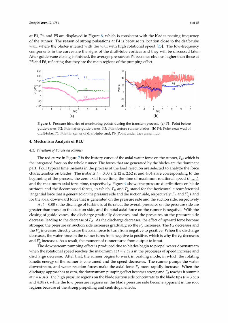
Figure 8 shows the pressure fluctuation histories at P1, P2, . . . , and P6. During the process ofguide-vane closure, the pressure at P1 increases gradually, while the pressures at P2 and P3 graduallydecrease, indicating water hammer characteristics. The pressure rise ratio at P1 is 39.18%, matching therequirement of less than 50% in Design code for small hydropower station in China [23]. The pressure at P3drops to its minimum −66.68 kPa, which is consistent with the results of reference [24]. When comparedwith the vaporization pressure value of −99.659 kPa at room temperature, there is a safety marginof 32.98 kPa, so no water column separation occurs during the load rejection process. The pressureat these points is greatly affected by the runner blades because P3 is near the inlet of runner blades,while P4 and P5 are near the outlet of runner blades (Figure 6). The high-frequency pressure pulsations

Energies 2019, 12, 4781 8 of 15

at P3, P4 and P5 are displayed in Figure 8, which is consistent with the blades passing frequencyof the runner. The reason of strong pulsations at P4 is because its location close to the draft-tubewall, where the blades interact with the wall with high rotational speed [25]. The low-frequencycomponents in the curves are the signs of the draft-tube vortices and they will be discussed later.After guide-vane closing is finished, the average pressure at P4 becomes obvious higher than those atP5 and P6, reflecting that they are the main regions of the pumping effect.

Energies 2019, 10, x FOR PEER REVIEW 8 of 15

gradually decrease, indicating water hammer characteristics. The pressure rise ratio at P1 is 39.18%, matching the requirement of less than 50% in Design code for small hydropower station in China [23]. The pressure at P3 drops to its minimum −66.68 kPa, which is consistent with the results of reference [24]. When compared with the vaporization pressure value of −99.659 kPa at room temperature, there is a safety margin of 32.98 kPa, so no water column separation occurs during the load rejection process. The pressure at these points is greatly affected by the runner blades because P3 is near the inlet of runner blades, while P4 and P5 are near the outlet of runner blades (Figure 6). The high-frequency pressure pulsations at P3, P4 and P5 are displayed in Figure 8, which is consistent with the blades passing frequency of the runner. The reason of strong pulsations at P4 is because its location close to the draft-tube wall, where the blades interact with the wall with high rotational speed [25]. The low-frequency components in the curves are the signs of the draft-tube vortices and they will be discussed later. After guide-vane closing is finished, the average pressure at P4 becomes obvious higher than those at P5 and P6, reflecting that they are the main regions of the pumping effect.

0 1 2 3 4 5 6 7-100

-50

0

50

100

150

200

250

P3

P2

P1

t (s)

P (

kPa)

0 1 2 3 4 5 6 7

-40

-20

0

20

40

60

t (s)

P6

P5

P4

P (

kPa)

(a) (b)

Figure 8. Pressure histories of monitoring points during the transient process. (a) P1: Point before guide-vanes; P2: Point after guide-vanes; P3: Point before runner blades. (b) P4: Point near wall of draft-tube; P5: Point in center of draft-tube; and, P6: Point under the runner hub.

4. Mechanism Analysis of RLU

4.1. Variation of Forces on Runner

The red curve in Figure 7 is the history curve of the axial water force on the runner, Fz, which is the integrated force on the whole runner. The forces that are generated by the blades are the dominant part. Four typical time instants in the process of the load rejection are selected to analyze the force characteristics on blades. The instants t = 0.00 s, 2.12 s, 2.52 s, and 4.04 s are corresponding to the beginning of the process, the zero axial force time, the time of maximum rotational speed (tnmax), and the maximum axial force time, respectively. Figure 9 shows the pressure distributions on blade surfaces and the decomposed forces, in which, Fθ and Fθ

' stand for the horizontal circumferential tangential force that is generated on the pressure side and the suction side, respectively; FA and FA

' stand for the axial downward force that is generated on the pressure side and the suction side, respectively.

At t = 0.00 s, the discharge of turbine is at its rated, the overall pressures on the pressure side are greater than those on the suction side, and the total axial force on the runner is negative. With the closing of guide-vanes, the discharge gradually decreases, and the pressures on the pressure side decrease, leading to the decrease of FA. As the discharge decreases, the effect of upward force become stronger, the pressure on suction side increases gradually, so the FA

' increases. The FA decreases and the FA

' increases directly cause the axial force to turn from negative to positive. When the discharge decreases, the water force on the runner turns from negative to positive, which is why the Fθ decreases and Fθ

' increases. As a result, the moment of runner turns from output to input. The downstream pumping effect is produced due to blades begin to propel water downstream

when the rotational speed reaches the maximum at t = 2.52 s in the processes of speed increase and discharge decrease. After that, the runner begins to work in braking mode, in which the rotating

Figure 8. Pressure histories of monitoring points during the transient process. (a) P1: Point beforeguide-vanes; P2: Point after guide-vanes; P3: Point before runner blades. (b) P4: Point near wall ofdraft-tube; P5: Point in center of draft-tube; and, P6: Point under the runner hub.

4. Mechanism Analysis of RLU

4.1. Variation of Forces on Runner

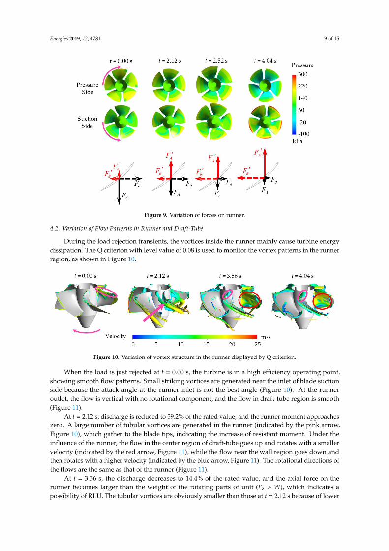
The red curve in Figure 7 is the history curve of the axial water force on the runner, Fz, which isthe integrated force on the whole runner. The forces that are generated by the blades are the dominantpart. Four typical time instants in the process of the load rejection are selected to analyze the forcecharacteristics on blades. The instants t = 0.00 s, 2.12 s, 2.52 s, and 4.04 s are corresponding to thebeginning of the process, the zero axial force time, the time of maximum rotational speed (tnmax),and the maximum axial force time, respectively. Figure 9 shows the pressure distributions on bladesurfaces and the decomposed forces, in which, Fθ and F′θ stand for the horizontal circumferentialtangential force that is generated on the pressure side and the suction side, respectively; FA and F′A standfor the axial downward force that is generated on the pressure side and the suction side, respectively.

At t = 0.00 s, the discharge of turbine is at its rated, the overall pressures on the pressure side aregreater than those on the suction side, and the total axial force on the runner is negative. With theclosing of guide-vanes, the discharge gradually decreases, and the pressures on the pressure sidedecrease, leading to the decrease of FA. As the discharge decreases, the effect of upward force becomestronger, the pressure on suction side increases gradually, so the F′A increases. The FA decreases andthe F′A increases directly cause the axial force to turn from negative to positive. When the dischargedecreases, the water force on the runner turns from negative to positive, which is why the Fθ decreasesand F′θ increases. As a result, the moment of runner turns from output to input.

The downstream pumping effect is produced due to blades begin to propel water downstreamwhen the rotational speed reaches the maximum at t = 2.52 s in the processes of speed increase anddischarge decrease. After that, the runner begins to work in braking mode, in which the rotatingkinetic energy of the runner is consumed and the speed decreases. The runner pumps the waterdownstream, and water reaction forces make the axial force Fz more rapidly increase. When thedischarge approaches to zero, the downstream pumping effect becomes strong and Fz reaches it summitat t = 4.04 s. The high pressure regions on the blade suction side concentrate to the blade tips (t = 3.56 sand 4.04 s), while the low pressure regions on the blade pressure side become apparent in the rootregions because of the strong propelling and centrifugal effects.

Energies 2019, 12, 4781 9 of 15

Energies 2019, 10, x FOR PEER REVIEW 9 of 15

kinetic energy of the runner is consumed and the speed decreases. The runner pumps the water downstream, and water reaction forces make the axial force Fz more rapidly increase. When the discharge approaches to zero, the downstream pumping effect becomes strong and Fz reaches it summit at t = 4.04 s. The high pressure regions on the blade suction side concentrate to the blade tips (t = 3.56 s and 4.04 s), while the low pressure regions on the blade pressure side become apparent in the root regions because of the strong propelling and centrifugal effects.

Figure 9. Variation of forces on runner.

4.2. Variation of Flow Patterns in Runner and Draft-Tube

During the load rejection transients, the vortices inside the runner mainly cause turbine energy dissipation. The Q criterion with level value of 0.08 is used to monitor the vortex patterns in the runner region, as shown in Figure 10.

Figure 10. Variation of vortex structure in the runner displayed by Q criterion.

When the load is just rejected at t = 0.00 s, the turbine is in a high efficiency operating point, showing smooth flow patterns. Small striking vortices are generated near the inlet of blade suction side because the attack angle at the runner inlet is not the best angle (Figure 10). At the runner outlet, the flow is vertical with no rotational component, and the flow in draft-tube region is smooth (Figure 11).

At t = 2.12 s, discharge is reduced to 59.2% of the rated value, and the runner moment approaches zero. A large number of tubular vortices are generated in the runner (indicated by the pink arrow, Figure 10), which gather to the blade tips, indicating the increase of resistant moment. Under the influence of the runner, the flow in the center region of draft-tube goes up and rotates with a smaller velocity (indicated by the red arrow, Figure 11), while the flow near the wall region

Figure 9. Variation of forces on runner.

4.2. Variation of Flow Patterns in Runner and Draft-Tube

During the load rejection transients, the vortices inside the runner mainly cause turbine energydissipation. The Q criterion with level value of 0.08 is used to monitor the vortex patterns in the runnerregion, as shown in Figure 10.

Energies 2019, 10, x FOR PEER REVIEW 9 of 15

kinetic energy of the runner is consumed and the speed decreases. The runner pumps the water downstream, and water reaction forces make the axial force Fz more rapidly increase. When the discharge approaches to zero, the downstream pumping effect becomes strong and Fz reaches it summit at t = 4.04 s. The high pressure regions on the blade suction side concentrate to the blade tips (t = 3.56 s and 4.04 s), while the low pressure regions on the blade pressure side become apparent in the root regions because of the strong propelling and centrifugal effects.

Figure 9. Variation of forces on runner.

4.2. Variation of Flow Patterns in Runner and Draft-Tube

During the load rejection transients, the vortices inside the runner mainly cause turbine energy dissipation. The Q criterion with level value of 0.08 is used to monitor the vortex patterns in the runner region, as shown in Figure 10.

Figure 10. Variation of vortex structure in the runner displayed by Q criterion.

When the load is just rejected at t = 0.00 s, the turbine is in a high efficiency operating point, showing smooth flow patterns. Small striking vortices are generated near the inlet of blade suction side because the attack angle at the runner inlet is not the best angle (Figure 10). At the runner outlet, the flow is vertical with no rotational component, and the flow in draft-tube region is smooth (Figure 11).

At t = 2.12 s, discharge is reduced to 59.2% of the rated value, and the runner moment approaches zero. A large number of tubular vortices are generated in the runner (indicated by the pink arrow, Figure 10), which gather to the blade tips, indicating the increase of resistant moment. Under the influence of the runner, the flow in the center region of draft-tube goes up and rotates with a smaller velocity (indicated by the red arrow, Figure 11), while the flow near the wall region

Figure 10. Variation of vortex structure in the runner displayed by Q criterion.

When the load is just rejected at t = 0.00 s, the turbine is in a high efficiency operating point,showing smooth flow patterns. Small striking vortices are generated near the inlet of blade suctionside because the attack angle at the runner inlet is not the best angle (Figure 10). At the runneroutlet, the flow is vertical with no rotational component, and the flow in draft-tube region is smooth(Figure 11).

At t = 2.12 s, discharge is reduced to 59.2% of the rated value, and the runner moment approacheszero. A large number of tubular vortices are generated in the runner (indicated by the pink arrow,Figure 10), which gather to the blade tips, indicating the increase of resistant moment. Under theinfluence of the runner, the flow in the center region of draft-tube goes up and rotates with a smallervelocity (indicated by the red arrow, Figure 11), while the flow near the wall region goes down andthen rotates with a higher velocity (indicated by the blue arrow, Figure 11). The rotational directions ofthe flows are the same as that of the runner (Figure 11).

At t = 3.56 s, the discharge decreases to 14.4% of the rated value, and the axial force on therunner becomes larger than the weight of the rotating parts of unit (Fz > W), which indicates apossibility of RLU. The tubular vortices are obviously smaller than those at t = 2.12 s because of lower

Energies 2019, 12, 4781 10 of 15

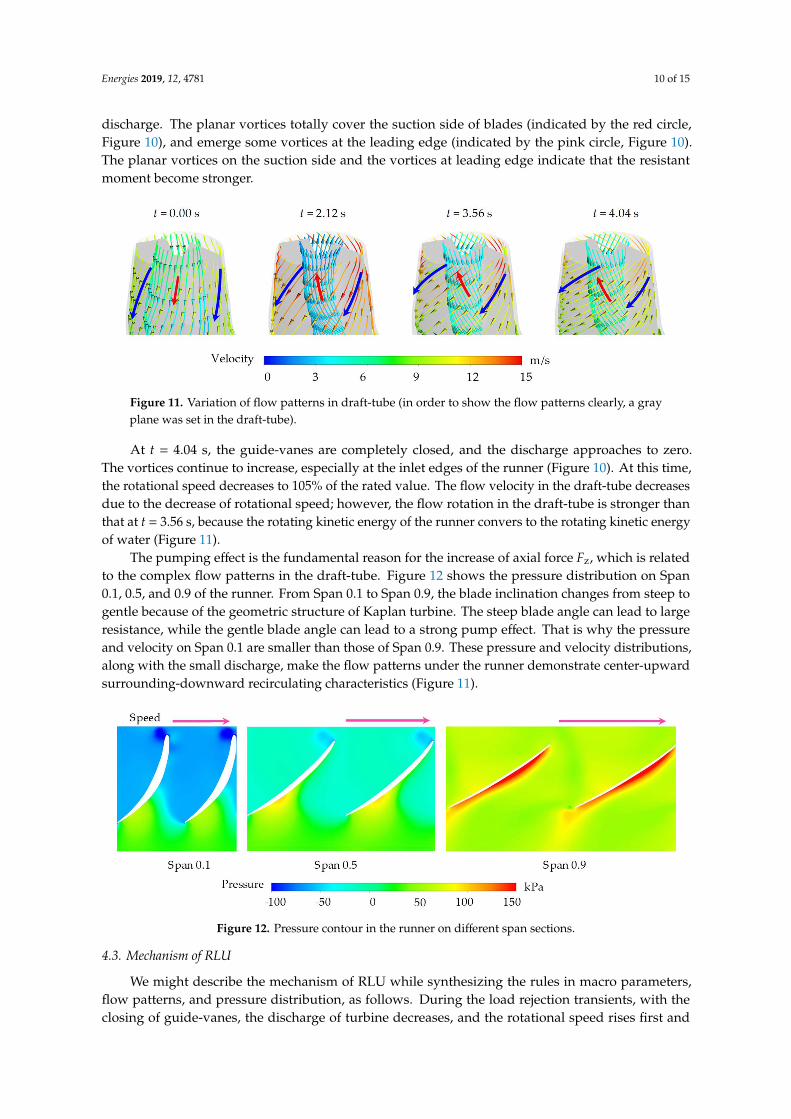
discharge. The planar vortices totally cover the suction side of blades (indicated by the red circle,Figure 10), and emerge some vortices at the leading edge (indicated by the pink circle, Figure 10).The planar vortices on the suction side and the vortices at leading edge indicate that the resistantmoment become stronger.

Energies 2019, 10, x FOR PEER REVIEW 10 of 15

goes down and then rotates with a higher velocity (indicated by the blue arrow, Figure 11). The rotational directions of the flows are the same as that of the runner (Figure 11).

Figure 11. Variation of flow patterns in draft-tube (in order to show the flow patterns clearly, a gray plane was set in the draft-tube).

At t = 3.56 s, the discharge decreases to 14.4% of the rated value, and the axial force on the runner becomes larger than the weight of the rotating parts of unit (Fz > W), which indicates a possibility of RLU. The tubular vortices are obviously smaller than those at t = 2.12 s because of lower discharge. The planar vortices totally cover the suction side of blades (indicated by the red circle, Figure 10), and emerge some vortices at the leading edge (indicated by the pink circle, Figure 10). The planar vortices on the suction side and the vortices at leading edge indicate that the resistant moment become stronger.

At t = 4.04 s, the guide-vanes are completely closed, and the discharge approaches to zero. The vortices continue to increase, especially at the inlet edges of the runner (Figure 10). At this time, the rotational speed decreases to 105% of the rated value. The flow velocity in the draft-tube decreases due to the decrease of rotational speed; however, the flow rotation in the draft-tube is stronger than that at t = 3.56 s, because the rotating kinetic energy of the runner convers to the rotating kinetic energy of water (Figure 11).

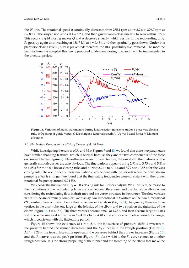
The pumping effect is the fundamental reason for the increase of axial force Fz, which is related to the complex flow patterns in the draft-tube. Figure 12 shows the pressure distribution on Span 0.1, 0.5, and 0.9 of the runner. From Span 0.1 to Span 0.9, the blade inclination changes from steep to gentle because of the geometric structure of Kaplan turbine. The steep blade angle can lead to large resistance, while the gentle blade angle can lead to a strong pump effect. That is why the pressure and velocity on Span 0.1 are smaller than those of Span 0.9. These pressure and velocity distributions, along with the small discharge, make the flow patterns under the runner demonstrate center-upward surrounding-downward recirculating characteristics (Figure 11).

Figure 12. Pressure contour in the runner on different span sections.

Figure 11. Variation of flow patterns in draft-tube (in order to show the flow patterns clearly, a grayplane was set in the draft-tube).

At t = 4.04 s, the guide-vanes are completely closed, and the discharge approaches to zero.The vortices continue to increase, especially at the inlet edges of the runner (Figure 10). At this time,the rotational speed decreases to 105% of the rated value. The flow velocity in the draft-tube decreasesdue to the decrease of rotational speed; however, the flow rotation in the draft-tube is stronger thanthat at t = 3.56 s, because the rotating kinetic energy of the runner convers to the rotating kinetic energyof water (Figure 11).

The pumping effect is the fundamental reason for the increase of axial force Fz, which is relatedto the complex flow patterns in the draft-tube. Figure 12 shows the pressure distribution on Span0.1, 0.5, and 0.9 of the runner. From Span 0.1 to Span 0.9, the blade inclination changes from steep togentle because of the geometric structure of Kaplan turbine. The steep blade angle can lead to largeresistance, while the gentle blade angle can lead to a strong pump effect. That is why the pressureand velocity on Span 0.1 are smaller than those of Span 0.9. These pressure and velocity distributions,along with the small discharge, make the flow patterns under the runner demonstrate center-upwardsurrounding-downward recirculating characteristics (Figure 11).

Energies 2019, 10, x FOR PEER REVIEW 10 of 15

goes down and then rotates with a higher velocity (indicated by the blue arrow, Figure 11). The rotational directions of the flows are the same as that of the runner (Figure 11).

Figure 11. Variation of flow patterns in draft-tube (in order to show the flow patterns clearly, a gray plane was set in the draft-tube).

At t = 3.56 s, the discharge decreases to 14.4% of the rated value, and the axial force on the runner becomes larger than the weight of the rotating parts of unit (Fz > W), which indicates a possibility of RLU. The tubular vortices are obviously smaller than those at t = 2.12 s because of lower discharge. The planar vortices totally cover the suction side of blades (indicated by the red circle, Figure 10), and emerge some vortices at the leading edge (indicated by the pink circle, Figure 10). The planar vortices on the suction side and the vortices at leading edge indicate that the resistant moment become stronger.

At t = 4.04 s, the guide-vanes are completely closed, and the discharge approaches to zero. The vortices continue to increase, especially at the inlet edges of the runner (Figure 10). At this time, the rotational speed decreases to 105% of the rated value. The flow velocity in the draft-tube decreases due to the decrease of rotational speed; however, the flow rotation in the draft-tube is stronger than that at t = 3.56 s, because the rotating kinetic energy of the runner convers to the rotating kinetic energy of water (Figure 11).

The pumping effect is the fundamental reason for the increase of axial force Fz, which is related to the complex flow patterns in the draft-tube. Figure 12 shows the pressure distribution on Span 0.1, 0.5, and 0.9 of the runner. From Span 0.1 to Span 0.9, the blade inclination changes from steep to gentle because of the geometric structure of Kaplan turbine. The steep blade angle can lead to large resistance, while the gentle blade angle can lead to a strong pump effect. That is why the pressure and velocity on Span 0.1 are smaller than those of Span 0.9. These pressure and velocity distributions, along with the small discharge, make the flow patterns under the runner demonstrate center-upward surrounding-downward recirculating characteristics (Figure 11).

Figure 12. Pressure contour in the runner on different span sections. Figure 12. Pressure contour in the runner on different span sections.

4.3. Mechanism of RLU

We might describe the mechanism of RLU while synthesizing the rules in macro parameters,flow patterns, and pressure distribution, as follows. During the load rejection transients, with theclosing of guide-vanes, the discharge of turbine decreases, and the rotational speed rises first and

Energies 2019, 12, 4781 11 of 15

then decreases. The runner will enter the downstream pumping mode, in which the runner propelswater downstream, because of the low discharge and high speed. The pressure on the pressure side ofrunner blades become lower, while the pressure on the suction side become higher, which produces alarger upward axial force Fz. Fz rapidly increases as discharge decreases sharply to a very low valueor even to zero. The RLU might occur if Fz exceeds the weight of rotating parts W. The maximalFz happens after discharge approaches to zero, because the pumping effect becomes larger withsmallest discharge and relative higher speed. After the summit, Fz decreases as the speed falls.When speed falls to a certain value, Fz will become smaller than W, which indicates the ending ofRLU. The simultaneous occurrence of low discharge and high speed is the reason of the pumpingeffect, which is also the reason for RLU. In the downstream pumping mode, the flow in the draft-tubedemonstrates center-upward surrounding-downward recirculating characteristics, and the vortices inthe runner shows complex structures.

5. Solution to the RLU Problem

5.1. Basic Idea on the Solution

Adjusting guide-vane closing rule is always the first considered means to solve the guaranteeregulation problems in load rejection transients of hydropower stations. Trying to reduce the axialwater force Fz, we first adjust only the closing time Ts, and found that Fz cannot be reduced apparentlywhen using a linear rule, no matter shortening or lengthening Ts. This is because the simultaneousoccurrence of low discharge and high speed cannot be avoided. Even the rated speed meeting a zerodischarge will generate a Fz that may cause RLU.

We proposed to suspend the closing after tnmax = 2.52 s for a certain period to reduce the speedby making use of the braking effect when considering the mechanism of large Fz, and knowing thatthe turbine is working in the braking mode after the maximum speed time tnmax = 2.52 s (Figure 7).If the suspending opening and time are proper, the speed can be reduced to a value that restrainsthe pumping effect to generate larger Fz. When Fz is kept low, the suspended closing can then becontinued until final closed.

This is a piecewise closing rule that can avoid the simultaneous occurrence of high speed and lowdischarge. The suspending period in the middle reach of the closing rule can reduce the speed andmake the zero discharge time tQmin far lag behind the maximum speed time tnmax.

The proper selections of the starting instant of suspending, the suspending opening, and thesuspending period are the keys to for using the above piecewise closing rule. The starting instant ofsuspending should be in between the maximum speed instant tnmax and the instant t1(Fz > W) whenFz > W first happens. The closer to t1(Fz > W) the faster the speed decreases. However, if we choset1(Fz > W) as the starting instant of suspending, the risk of RLU might exist. Therefore, a margin shouldbe left. When the starting instant is set, we will then know the corresponding opening by following theoriginal linear closing rule. The suspending might be ended when the reduced speed is smaller thanthe speed value at t2(Fz > W) when Fz > W ends; therefore, the suspending period is certainly largerthan the period of Fz > W. The suspending period can be determined by trial and error simulations,and it should be extended to further reduce the speed to a lower value for safety margin.

5.2. Feasibility Verification with the Piecewise Closing Rule

For the Ts = 4.0 s linear closing rule in Figure 7, tnmax = 2.5 s, t1(Fz > W) = 3.57 s and t2(Fz > W) = 6.13 s.We made several trial and error simulations and selected a proper piecewise rule, with the startinginstant t = 3.2 s, the suspending period 5.0 s, and the total closing time Ts = 9.0 s, as shown in Figure 13.

The macro-parameter histories from 0.0 s to 3.2 s are consistent with those for the original closingrule depicted in Figure 7. After the guide-vane opening is suspended at t = 3.2 s, the discharge Q firsthas a slight disturbance and then keeps stable at around 2.96 m3/s. The axial water force Fz continuesto rise first and then gradually falls, with the highest value 139.2 kN at t = 3.66 s, nearly touching

Energies 2019, 12, 4781 12 of 15

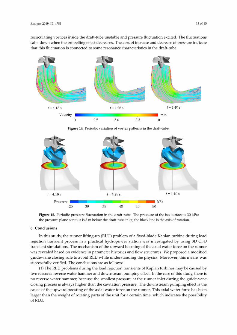
the W line. The rotational speed n continually decreases from 285.1 rpm at t = 3.2 s to 229.7 rpm att = 8.2 s. The suspension stops at t = 8.2 s, and then guide-vanes close linearly to zero within 0.72 s.This second rapid closing makes Q and n decrease sharply, which results in the rebounding of Fz.Fz goes up again until reaching at 138.7 kN at t = 9.43 s, and then gradually goes down. Under thispiecewise closing rule, Fz > W is prevented; therefore, the RLU possibility is eliminated. The machinemanufacturer has accepted this newly proposed guide-vane closing rule, and it will be implemented inthe practical project.Energies 2019, 10, x FOR PEER REVIEW 12 of 15

0 1 2 3 4 5 6 7 8 9 10 11 120

5

10

15

20

25

30

35

40a(º) Fz(kN)

Q(m3/s) M(kNm)n(rpm)

t (s)

aQn

140

0

2

4

6

8

10

12

14

16

140

160

180

200

220

240

260

280

300

-100

-50

0

50

100

150

200Fz

-100

-75

-50

-25

0

25

50

75

100M

Figure 13. Variation of macro-parameters during load rejection transients under a piecewise closing rule. α Opening of guide-vanes; Q Discharge; n Rational speed; FZ Upward axial force; M Moment of runner.

The macro-parameter histories from 0.0 s to 3.2 s are consistent with those for the original closing rule depicted in Figure 7. After the guide-vane opening is suspended at t = 3.2 s, the discharge Q first has a slight disturbance and then keeps stable at around 2.96 m3/s. The axial water force Fz continues to rise first and then gradually falls, with the highest value 139.2 kN at t = 3.66 s, nearly touching the W line. The rotational speed n continually decreases from 285.1 rpm at t = 3.2 s to 229.7 rpm at t = 8.2 s. The suspension stops at t = 8.2 s, and then guide-vanes close linearly to zero within 0.72 s. This second rapid closing makes Q and n decrease sharply, which results in the rebounding of Fz. Fz goes up again until reaching at 138.7 kN at t = 9.43 s, and then gradually goes down. Under this piecewise closing rule, Fz > W is prevented; therefore, the RLU possibility is eliminated. The machine manufacturer has accepted this newly proposed guide-vane closing rule, and it will be implemented in the practical project.

5.3. Fluctuation Reasons in the History Curves of Axial Force

While investigating the curves of Fz and M in Figure 7 and Figure 13, we found that these two parameters have similar changing features, which is normal because they are the two components of the force on runner blades (Figure 9). Nevertheless, as an unusual feature, the saw-tooth fluctuations on the generally smooth curves are also obvious. The fluctuations appear during 2.91 s to 3.73 s and 5.61 s to 6.85 s for the 4.0 s linear closing rule, and during 2.91 s to 6.14 s and 8.79 s to 10.55 s for the 9.0 s closing rule. The occurrence of these fluctuations is coincident with the periods when the downstream pumping effect is stronger. We found that the fluctuating frequencies were consistent with the runner rotational frequency around 0.24 Hz.

We choose the fluctuation in Ts = 9.0 s closing rule for further analysis. We attributed the reason to the fluctuations of the recirculating large vortices between the runner and the draft-tube elbow when considering the recirculating flow in draft-tube and the vortex structure in the runner. The flow vortices in draft-tube are extremely complex. We display two-dimensional 3D vortices on the two-dimensional (2D) central plane of draft-tube for the convenience of analysis (Figure 14). In general, there are three vortices in the draft-tube, one large on the left side of the elbow and two small on the right side of the elbow (Figure 14, t = 4.18 s). The three vortices become small at 4.28 s, and then become large at 4.40 s with the same size as at 4.18 s. From t = 4.18 s to t = 4.40 s, the vortices complete a period of changes, which is consistent with the fluctuating period.

Figure 13. Variation of macro-parameters during load rejection transients under a piecewise closingrule. α Opening of guide-vanes; Q Discharge; n Rational speed; FZ Upward axial force; M Momentof runner.

5.3. Fluctuation Reasons in the History Curves of Axial Force

While investigating the curves of Fz and M in Figures 7 and 13, we found that these two parametershave similar changing features, which is normal because they are the two components of the forceon runner blades (Figure 9). Nevertheless, as an unusual feature, the saw-tooth fluctuations on thegenerally smooth curves are also obvious. The fluctuations appear during 2.91 s to 3.73 s and 5.61 sto 6.85 s for the 4.0 s linear closing rule, and during 2.91 s to 6.14 s and 8.79 s to 10.55 s for the 9.0 sclosing rule. The occurrence of these fluctuations is coincident with the periods when the downstreampumping effect is stronger. We found that the fluctuating frequencies were consistent with the runnerrotational frequency around 0.24 Hz.

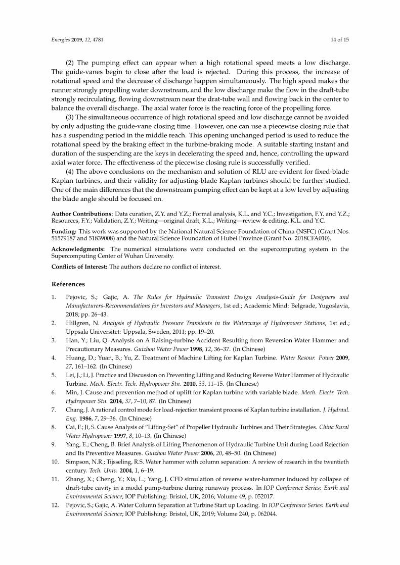
We choose the fluctuation in Ts = 9.0 s closing rule for further analysis. We attributed the reason tothe fluctuations of the recirculating large vortices between the runner and the draft-tube elbow whenconsidering the recirculating flow in draft-tube and the vortex structure in the runner. The flow vorticesin draft-tube are extremely complex. We display two-dimensional 3D vortices on the two-dimensional(2D) central plane of draft-tube for the convenience of analysis (Figure 14). In general, there are threevortices in the draft-tube, one large on the left side of the elbow and two small on the right side of theelbow (Figure 14, t = 4.18 s). The three vortices become small at 4.28 s, and then become large at 4.40 swith the same size as at 4.18 s. From t = 4.18 s to t = 4.40 s, the vortices complete a period of changes,which is consistent with the fluctuating period.

Figure 15 shows the evidence, at t = 4.18 s, the iso-surface of pressure shifts downstream,the pressure behind the runner decreases, and the Fz curve is in the trough position (Figure 13).At t = 4.28 s, the iso-surface shifts upstream, the pressure behind the runner increases (Figure 15),and the Fz curve is at the peak position (Figure 13). At t = 4.40 s, the Fz curve comes to anothertrough position. It is the strong propelling of the runner and the throttling of the elbow that make the

Energies 2019, 12, 4781 13 of 15

recirculating vortices inside the draft-tube unstable and pressure fluctuation excited. The fluctuationscalm down when the propelling effect decreases. The abrupt increase and decrease of pressure indicatethat this fluctuation is connected to some resonance characteristics in the draft-tube.Energies 2019, 10, x FOR PEER REVIEW 13 of 15

Figure 14. Periodic variation of vortex patterns in the draft-tube.

Figure 15 shows the evidence, at t = 4.18 s, the iso-surface of pressure shifts downstream, the pressure behind the runner decreases, and the Fz curve is in the trough position (Figure 13). At t = 4.28 s, the iso-surface shifts upstream, the pressure behind the runner increases (Figure 15), and the Fz curve is at the peak position (Figure 13). At t = 4.40 s, the Fz curve comes to another trough position. It is the strong propelling of the runner and the throttling of the elbow that make the recirculating vortices inside the draft-tube unstable and pressure fluctuation excited. The fluctuations calm down when the propelling effect decreases. The abrupt increase and decrease of pressure indicate that this fluctuation is connected to some resonance characteristics in the draft-tube.

Figure 15. Periodic pressure fluctuation in the draft-tube. The pressure of the iso-surface is 30 kPa; the pressure plane contour is 3 m below the draft-tube inlet; the black line is the axis of rotation.

6. Conclusions

In this study, the runner lifting-up (RLU) problem of a fixed-blade Kaplan turbine during load rejection transient process in a practical hydropower station was investigated by using 3D CFD transient simulations. The mechanism of the upward boosting of the axial water force on the runner was revealed based on evidence in parameter histories and flow structures. We proposed a modified guide-vane closing rule to avoid RLU while understanding the physics. Moreover, this means was successfully verified. The conclusions are as follows:

(1) The RLU problems during the load rejection transients of Kaplan turbines may be caused by two reasons: reverse water hammer and downstream pumping effect. In the case of this study, there is no reverse water hammer, because the smallest pressure at the runner inlet during the guide-vane

Figure 14. Periodic variation of vortex patterns in the draft-tube.

Energies 2019, 10, x FOR PEER REVIEW 13 of 15

Figure 14. Periodic variation of vortex patterns in the draft-tube.

Figure 15 shows the evidence, at t = 4.18 s, the iso-surface of pressure shifts downstream, the pressure behind the runner decreases, and the Fz curve is in the trough position (Figure 13). At t = 4.28 s, the iso-surface shifts upstream, the pressure behind the runner increases (Figure 15), and the Fz curve is at the peak position (Figure 13). At t = 4.40 s, the Fz curve comes to another trough position. It is the strong propelling of the runner and the throttling of the elbow that make the recirculating vortices inside the draft-tube unstable and pressure fluctuation excited. The fluctuations calm down when the propelling effect decreases. The abrupt increase and decrease of pressure indicate that this fluctuation is connected to some resonance characteristics in the draft-tube.

Figure 15. Periodic pressure fluctuation in the draft-tube. The pressure of the iso-surface is 30 kPa; the pressure plane contour is 3 m below the draft-tube inlet; the black line is the axis of rotation.

6. Conclusions

In this study, the runner lifting-up (RLU) problem of a fixed-blade Kaplan turbine during load rejection transient process in a practical hydropower station was investigated by using 3D CFD transient simulations. The mechanism of the upward boosting of the axial water force on the runner was revealed based on evidence in parameter histories and flow structures. We proposed a modified guide-vane closing rule to avoid RLU while understanding the physics. Moreover, this means was successfully verified. The conclusions are as follows:

(1) The RLU problems during the load rejection transients of Kaplan turbines may be caused by two reasons: reverse water hammer and downstream pumping effect. In the case of this study, there is no reverse water hammer, because the smallest pressure at the runner inlet during the guide-vane

Figure 15. Periodic pressure fluctuation in the draft-tube. The pressure of the iso-surface is 30 kPa;the pressure plane contour is 3 m below the draft-tube inlet; the black line is the axis of rotation.

6. Conclusions

In this study, the runner lifting-up (RLU) problem of a fixed-blade Kaplan turbine during loadrejection transient process in a practical hydropower station was investigated by using 3D CFDtransient simulations. The mechanism of the upward boosting of the axial water force on the runnerwas revealed based on evidence in parameter histories and flow structures. We proposed a modifiedguide-vane closing rule to avoid RLU while understanding the physics. Moreover, this means wassuccessfully verified. The conclusions are as follows:

(1) The RLU problems during the load rejection transients of Kaplan turbines may be caused bytwo reasons: reverse water hammer and downstream pumping effect. In the case of this study, there isno reverse water hammer, because the smallest pressure at the runner inlet during the guide-vaneclosing process is always higher than the cavitation pressure. The downstream pumping effect is thecause of the upward boosting of the axial water force on the runner. This axial water force has beenlarger than the weight of rotating parts of the unit for a certain time, which indicates the possibilityof RLU.

Energies 2019, 12, 4781 14 of 15

(2) The pumping effect can appear when a high rotational speed meets a low discharge.The guide-vanes begin to close after the load is rejected. During this process, the increase ofrotational speed and the decrease of discharge happen simultaneously. The high speed makes therunner strongly propelling water downstream, and the low discharge make the flow in the draft-tubestrongly recirculating, flowing downstream near the drat-tube wall and flowing back in the center tobalance the overall discharge. The axial water force is the reacting force of the propelling force.

(3) The simultaneous occurrence of high rotational speed and low discharge cannot be avoidedby only adjusting the guide-vane closing time. However, one can use a piecewise closing rule thathas a suspending period in the middle reach. This opening unchanged period is used to reduce therotational speed by the braking effect in the turbine-braking mode. A suitable starting instant andduration of the suspending are the keys in decelerating the speed and, hence, controlling the upwardaxial water force. The effectiveness of the piecewise closing rule is successfully verified.

(4) The above conclusions on the mechanism and solution of RLU are evident for fixed-bladeKaplan turbines, and their validity for adjusting-blade Kaplan turbines should be further studied.One of the main differences that the downstream pumping effect can be kept at a low level by adjustingthe blade angle should be focused on.

Author Contributions: Data curation, Z.Y. and Y.Z.; Formal analysis, K.L. and Y.C.; Investigation, F.Y. and Y.Z.;Resources, F.Y.; Validation, Z.Y.; Writing—original draft, K.L.; Writing—review & editing, K.L. and Y.C.

Funding: This work was supported by the National Natural Science Foundation of China (NSFC) (Grant Nos.51579187 and 51839008) and the Natural Science Foundation of Hubei Province (Grant No. 2018CFA010).

Acknowledgments: The numerical simulations were conducted on the supercomputing system in theSupercomputing Center of Wuhan University.

Conflicts of Interest: The authors declare no conflict of interest.

References

1. Pejovic, S.; Gajic, A. The Rules for Hydraulic Transient Design Analysis-Guide for Designers andManufacturers-Recommendations for Investors and Managers, 1st ed.; Academic Mind: Belgrade, Yugoslavia,2018; pp. 26–43.

2. Hillgren, N. Analysis of Hydraulic Pressure Transients in the Waterways of Hydropower Stations, 1st ed.;Uppsala Universitet: Uppsala, Sweden, 2011; pp. 19–20.

3. Han, Y.; Liu, Q. Analysis on A Raising-turbine Accident Resulting from Reversion Water Hammer andPrecautionary Measures. Guizhou Water Power 1998, 12, 36–37. (In Chinese)

4. Huang, D.; Yuan, B.; Yu, Z. Treatment of Machine Lifting for Kaplan Turbine. Water Resour. Power 2009,27, 161–162. (In Chinese)

5. Lei, J.; Li, J. Practice and Discussion on Preventing Lifting and Reducing Reverse Water Hammer of HydraulicTurbine. Mech. Electr. Tech. Hydropower Stn. 2010, 33, 11–15. (In Chinese)

6. Min, J. Cause and prevention method of uplift for Kaplan turbine with variable blade. Mech. Electr. Tech.Hydropower Stn. 2014, 37, 7–10, 87. (In Chinese)

7. Chang, J. A rational control mode for load-rejection transient process of Kaplan turbine installation. J. Hydraul.Eng. 1986, 7, 29–36. (In Chinese)

8. Cai, F.; Ji, S. Cause Analysis of “Lifting-Set” of Propeller Hydraulic Turbines and Their Strategies. China RuralWater Hydropower 1997, 8, 10–13. (In Chinese)

9. Yang, E.; Cheng, B. Brief Analysis of Lifting Phenomenon of Hydraulic Turbine Unit during Load Rejectionand Its Preventive Measures. Guizhou Water Power 2006, 20, 48–50. (In Chinese)

10. Simpson, N.R.; Tijsseling, R.S. Water hammer with column separation: A review of research in the twentiethcentury. Tech. Univ. 2004, 1, 6–19.

11. Zhang, X.; Cheng, Y.; Xia, L.; Yang, J. CFD simulation of reverse water-hammer induced by collapse ofdraft-tube cavity in a model pump-turbine during runaway process. In IOP Conference Series: Earth andEnvironmental Science; IOP Publishing: Bristol, UK, 2016; Volume 49, p. 052017.

12. Pejovic, S.; Gajic, A. Water Column Separation at Turbine Start up Loading. In IOP Conference Series: Earth andEnvironmental Science; IOP Publishing: Bristol, UK, 2019; Volume 240, p. 062044.

Energies 2019, 12, 4781 15 of 15

13. Dudlik, A.; Koutnik, J. Water hammer 2 phase analysis hydraulic system with a Kaplan turbine. Kaplan Turbine2019, 10, 613–624.

14. Carija, Z.; Mrša, Z.; Dragovic, L. Turbulent Flow Simulation in Kaplan Draft Tube. In Proceedings of the5th International Congress of Croatian Society of Mechanics, Trogir/Split, Croatia, 21–23 September 2006;pp. 21–23.

15. Drtina, P.; Sallaberger, M. Hydraulic turbines—Basic principles and state-of-the-art computational fluiddynamics applications. J. Mech. Eng. Sci. 1999, 213, 85–102. [CrossRef]

16. Liu, S.; Wu, Y.; Jie, S.; Wu, S. Numerical simulation of pressure fluctuation in Kaplan turbine. Sci. China 2008,51, 1137–1148. [CrossRef]

17. Liu, S.; Zhou, D.; Liu, D.; Wu, Y.; Nishi, M. Runaway transient simulation of a model Kaplan turbine. In IOPConference Series: Earth and Environmental Science; IOP Publishing: Bristol, UK, 2010; Volume 12, p. 012073.

18. Yang, Z.; Cheng, Y.; Xia, L.; You, J. 3D numerical simulation of load rejection transients of a bulb hydraulicturbine. Eng. J. Wuhan Univ. 2018, 51, 854–860, 875. (In Chinese)

19. Chen, H.; Zhou, D.; Zheng, Y.; Jiang, S.; Yu, A.; Guo, Y. Load Rejection Transient Process Simulation of aKaplan Turbine Model by Co-Adjusting Guide Vanes and Runner Blades. Energies 2018, 11, 3354. [CrossRef]

20. Xia, L.; Cheng, Y.; Yang, Z.; You, J.; Yang, J.; Qian, Z. Evolutions of Pressure Fluctuations and Runner Loadsduring Runaway Processes of a Pump-Turbine. J. Fluids Eng. 2017, 139, 091101. [CrossRef]

21. Zhang, X.; Cheng, Y.; Yang, J.; Xia, L.; Lai, X. Simulation of the load rejection transient process of a Francisturbine by using a 1-D-3-D coupling approach. J. Hydrodyn. 2014, 26, 715–724. [CrossRef]

22. Yang, Z.; Cheng, Y.; Fang, C. Three-dimensional CFD simulation of the load rejection transient processconsidering regulating system. In IOP Conference Series: Earth and Environmental Science; IOP Publishing:Bristol, UK, 2018; Volume 163, p. 012079.

23. China Renewable Energy Engineering Institute; Sichuan Water Resources and Hydroelectric Investigation& Design Institute. Speed control system and regulation guarantee calculation. In Design Code for SmallHydropower Station; Jihua Press of China: Beijing, China, 2014; p. 39.

24. Liu, Y.; Chang, J. Study on Reverse Water Hammer of the Kaplan Turbine. Adv. Water Resour. Hydraul. Eng.2009, 1, 2208–2213.

25. Zheng, X.; Luo, X.; Guo, P. Analysis of Pressure Fluctuation in Draft Tube of Kaplan Turbine. Sci. Rep. 2009,1, 341–344.

© 2019 by the authors. Licensee MDPI, Basel, Switzerland. This article is an open accessarticle distributed under the terms and conditions of the Creative Commons Attribution(CC BY) license (http://creativecommons.org/licenses/by/4.0/).