RTL to Transistor Level Power Modelling and Estimation ...

HAL Id: hal-02866921https://hal.archives-ouvertes.fr/hal-02866921

Submitted on 12 Jun 2020

HAL is a multi-disciplinary open accessarchive for the deposit and dissemination of sci-entific research documents, whether they are pub-lished or not. The documents may come fromteaching and research institutions in France orabroad, or from public or private research centers.

L’archive ouverte pluridisciplinaire HAL, estdestinée au dépôt et à la diffusion de documentsscientifiques de niveau recherche, publiés ou non,émanant des établissements d’enseignement et derecherche français ou étrangers, des laboratoirespublics ou privés.

RTL to Transistor Level Power Modelling andEstimation Techniques for FPGA and ASIC: A SurveyYehya Nasser, Jordane Lorandel, Jean-Christophe Prevotet, Maryline Hélard

To cite this version:Yehya Nasser, Jordane Lorandel, Jean-Christophe Prevotet, Maryline Hélard. RTL to TransistorLevel Power Modelling and Estimation Techniques for FPGA and ASIC: A Survey. IEEE Transac-tions on Computer-Aided Design of Integrated Circuits and Systems, IEEE, 2021, 40 (3), pp.479-493.�10.1109/TCAD.2020.3003276�. �hal-02866921�

https://hal.archives-ouvertes.fr/hal-02866921

https://hal.archives-ouvertes.fr

IEEE TCAD CIRCUITS AND SYSTEMS 1

RTL to Transistor Level Power Modelling andEstimation Techniques for FPGA and ASIC: A

SurveyYehya Nasser, Jordane Lorandel, Jean-Christophe Prevotet, and Maryline Helard

Abstract—Power consumption constitutes a major challengefor electronics circuits. One possible way to deal with this issueis to consider it very soon in the design process in order to explorevarious design choices. A typical design flow often starts with ahigh-level description of a full system, which imposes to provideaccurate models. Power modelling techniques can be employed,providing a way to find a relationship between power and othermetrics. Furthermore, it is also important to consider efficientpower characterization techniques. The role of this paper is, first,to provide an overview of RTL to transistor level power modellingand estimation techniques for FPGAs and ASICs devices. Second,it aims at proposing a classification of all approaches accordingto defined metrics, which should help designers in finding aparticular method for their specific situation, even if no commonreference is defined among the considered works.

Index Terms—Power consumption, power modelling, powerestimation, high-level power estimation, FPGA, ASIC, tools.

I. INTRODUCTION

W ITH the imminent arrival of 5G and Internet of Things(IoT), a lot of electronic devices will be able to com-

municate and share data between them, involving machine tomachine or machine to vehicular communications for example.All sectors are concerned, starting from the industries to theagriculture, telecommunication, health, etc. . Human activitiesand technologies have a significant impact of the worldwidecarbon footprint. It has been shown that cities cover 2% ofEarth’s surface but consume up to 78% of the world’s energy[1]. In the same time, it has been shown that developing smartand energy-efficient technologies may be an efficient solutionto drastically reduce the energy cost and the environmentalimpact. These electronic devices are generally designed usinga Very-Large-Scale Integration (VLSI) process that consistsin building an integrated circuit (IC) by linking millions oftransistors on a chip. All complex systems and communicationdevices are based on VLSI, including analog ICs such assensors and operational amplifiers as well as digital ICs,such as microprocessors, Digital Signal Processors (DSPs),micro-controllers. In addition to this, VLSI design coversthe development of Application Specific Integrated Circuits(ASIC) and Programmable Logic (PL) Devices.

In this paper, we propose a taxonomy that is illustrated inFig. 1. This classification tends to facilitate the comparison ofmany circuits according to their hardware architectures. Twomain VLSI categories have been identified: hardware-definedand programmable hardware devices.

Hardware-defined devices can be then divided intoapplication-specific (e.g. ASIC) and non-application specific

VLSI

Non Application Specific

HW optimized

Programmable HW IC

-DSP-GPU-MPPA

-GPP-μC

Homogeneous HW

Heterogeneous HW

-FPGA-CPLD-SoPC

-SoC (e.g. Zynq)

Hardware-defined IC

-Standard Cell / Full custom ASICs-Gate Array

Application Specific

Fig. 1. Taxonomy on VLSI Integrated Circuits

ICs. We further divide the non-application specific devices intohardware-optimized for which GPU is an illustrative exampleand general ICs including General Purpose Processor (GPP)or micro-controllers. Regarding programmable hardware ICs,two categories have been defined depending on if the deviceis built from homogeneous hardware e.g. Field ProgrammableGate Array (FPGA) or heterogeneous resources. A System onChip (SoC) is a typical example of heterogeneous hardwareICs that contain a hard processor in combination with logicinto the same chip.

Nowadays, FPGAs are used in many applications, fromdata-centers to low-power smart embedded devices. Depend-ing on the application requirements, such devices can nowsupport complex designs, allowing fast prototyping and re-ducing time-to-market. FPGAs are popular in many sectorssuch as telecommunications, robotics, automotive, etc. .

A major feature of FPGAs is reconfiguration. As a conse-quence, FPGAs consume much more power than their ASICcounterparts as additional transistors are used to maintain thereconfiguration plan. Note that several FPGA technologiesexist such as SRAM or FLASH. The Flash technology isdedicated to low-power applications for specific segments ofthe market whereas SRAM technology is most common.

In this paper, we tackle the issues related to power mod-elling and estimation of both FPGAs and ASICs. In particular,we focus on CMOS and SRAM technologies, and do notconsider the flash technology that is specific. Several surveyshave already reviewed associated works [2],[3],[4],[5] but noneof them provides a way to compare power estimation andmodelling techniques between them. This prevents designersto rapidly identify the appropriate methods according to theirconstraints. Moreover, this paper focuses on RTL to transistorlevel power modelling and estimation techniques, rather than


system-level. Interested readers could refer to [6] for higherlevel techniques as Transaction-level power modelling.

The objectives of this survey are:

• to deliver a comparative study, including power mea-surement methods, commercial power estimation toolsand power modelling techniques. The comparison isperformed based on custom selected metrics.

• to help designers in identifying the most appropriatetechnique to estimate/measure the power consumption oftheir FPGA or ASIC design.

The paper is organized as follows: we first propose abackground on ASIC and FPGA devices in section II. Then,related works on power measurement techniques are givenin section VI. Section VI presents various power modellingapproaches. We finally present a comparison between themand conclude.

II. HARDWARE PLATFORMS

Before addressing the power issue for ASICs and FPGAs,the following subsections provide an overview of the hardwarearchitecture of each devices.

A. ASIC Architecture

ASICs consist of integrated circuits that are specificallybuilt for predefined functions. They can be classified into twocategories: full-Custom and semi-custom ASICs.

Full-Custom ASICs are customized and optimized circuitsthat offer the highest performance and the smallest die size.The design time is thus very long (up to several years forproduction) and the development costs are very high. Analternative to full-custom ASICs is denoted semicustom ASICsand helps designers to shorten the design time, to reducecosts and to automate the design process. This technology isbased on a regular organisation of homogeneous cells or theintegration of standard cells already defined in a library.

B. FPGA Architecture

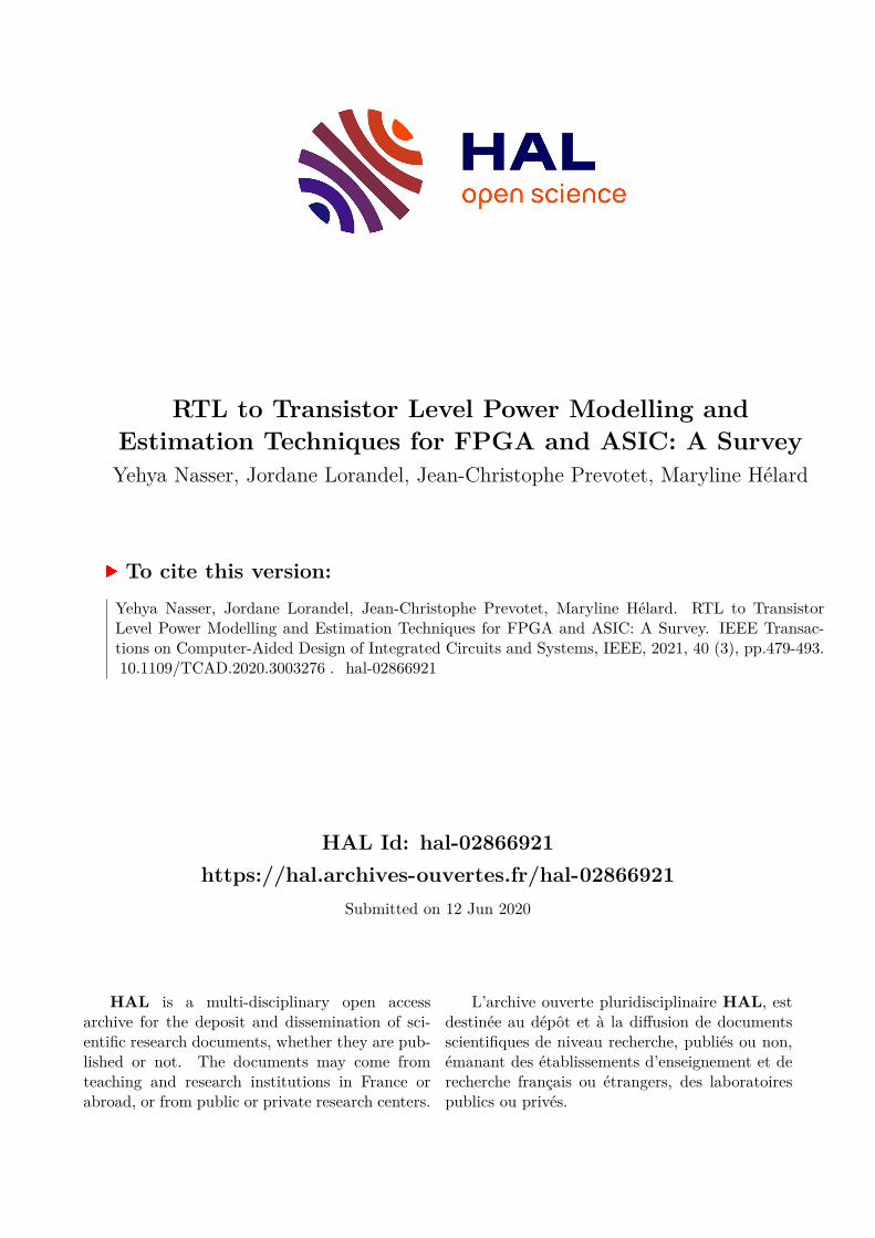
An FPGA architecture consists of a two dimensional arrayof configurable logic cells, inputs/outputs and interconnectionbetween them, as illustrated by Fig. 2. The basic internalstructure of a logic cell generally consists of look-up tables(LUT) implemented as memories. Each n-input LUT canimplement any function with up to n variables and consists of2n SRAM bits that store the required boolean truth table. Inaddition, there is at least a multiplexer and a flip-flop withineach cell. Each FPGA vendor proposes its own implementationof logic cells.They also may differ regarding the layout oftheir interconnect and the architecture of their configurableelements. FPGA devices can also integrate specific elements,such as Digital Signal Processors (DSP) blocks, RAM mem-ories, frequency synthesizers (PLL), as well as more sophisti-cated elements such as PCIe hardware controller, high speedcommunication transceivers etc. .

. Antifuse Technology (e.g., ActelTM, QuicklogicTM): an antifuse remains in a

high-impedance state until it is programmed into a low-impedance or “fused”

state (Figure 9.18). This technology can be used only once on one-time

programmable (OTP) devices; it is less expensive than the RAM technology.

. EPROM/EEPROM Technology (various PLDs): this method is the same as that

used in EPROM/EEPROM memories. The configuration is stored within the

device, that is, without external memory. Generally, in-circuit reprogramming

is not possible.

Look-Up Tables The way logic functions are implemented in a FPGA is another

key feature. Logic blocks that carry out logical functions are look-up tables

(LUTs), implemented as memory, or multiplexer and memory. Figure 9.19 shows

these alternatives, together with an example of memory contents for some basic

operations. A 2n � 1 ROM can implement any n-bit function. Typical sizes for n

are 2, 3, 4, or 5.

In Figure 9.19a, an n-bit LUT is implemented as a 2n�1 memory; the input

address selects one of 2nmemory locations. The memory locations (latches) are nor-

mally loaded with values from the user’s configuration bit-stream. In Figure 9.19b,

Programmableinput / output

Programmablebasic logic block

Programmableinterconnections

Figure 9.17 Basic architecture of FPGA: two-dimensional array of programmable logic

cells, interconnections, and input/ouput.

SR

AM

(a)Temporary high voltage

creates permanent shortcircuit

(b)

Figure 9.18 Programming methods: (a) SRAM connection and (b) antifuse.

9.4 PROGRAMMABLE LOGIC 259

Fig. 2. Basic FPGA architecture [7]

Design Synthesis

Specification

RTL Modeling

Design Implementation

Post-Synthesis Power Estimation

Post-P&R Power Estimation

Power Measurement

Bitstream Generation

Device Configuration

Power Consumption Evaluation

Verificatio

n

Valid

ation

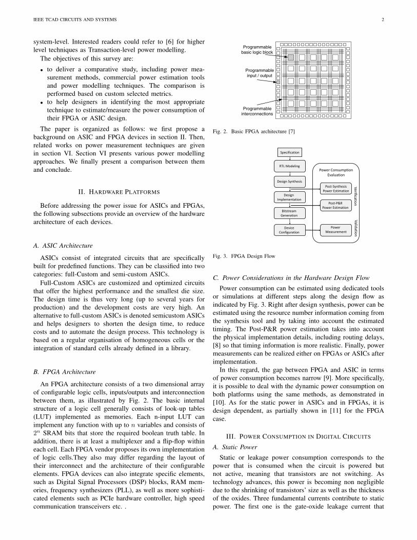
Fig. 3. FPGA Design Flow

C. Power Considerations in the Hardware Design Flow

Power consumption can be estimated using dedicated toolsor simulations at different steps along the design flow asindicated by Fig. 3. Right after design synthesis, power can beestimated using the resource number information coming fromthe synthesis tool and by taking into account the estimatedtiming. The Post-P&R power estimation takes into accountthe physical implementation details, including routing delays,[8] so that timing information is more realistic. Finally, powermeasurements can be realized either on FPGAs or ASICs afterimplementation.

In this regard, the gap between FPGA and ASIC in termsof power consumption becomes narrow [9]. More specifically,it is possible to deal with the dynamic power consumption onboth platforms using the same methods, as demonstrated in[10]. As for the static power in ASICs and in FPGAs, it isdesign dependent, as partially shown in [11] for the FPGAcase.

III. POWER CONSUMPTION IN DIGITAL CIRCUITS

A. Static Power

Static or leakage power consumption corresponds to thepower that is consumed when the circuit is powered butnot active, meaning that transistors are not switching. Astechnology advances, this power is becoming non negligibledue to the shrinking of transistors’ size as well as the thicknessof the oxides. Three fundamental currents contribute to staticpower. The first one is the gate-oxide leakage current that


occurs between the transistor’s channel and gate. The secondis the sub-threshold leakage current that occurs between thetransistor’s source and drain. The last contributor is the reversebias current, which is located between the transistor’s drainand the substrate. When considering high-k dielectric devices,the main source of static power remains the sub-thresholdleakage current Ileakage [12] and it can be expressed as:

Ileakage = I0e−qVthβkBT (1)

where

– I0 denotes a constant that depends on the dimension andthe fabrication technology of the transistor;

– β is a technology-dependent factor;– kB stands for the Boltzmann constant;– T represents the temperature;– q represents the charge of the electrical carrier;– Vth represents the threshold voltage.

Depending on a given technology, temperature and thresholdvoltage have an exponential impact on leakage currents andthus on static power since Pstatic = VddIleakage, where Vddrepresents the supply voltage.

B. Dynamic Power

In current digital circuits, dynamic power remains the mainsource of power consumption. This source of power consump-tion is generated by the transistors’ switching activity whenthe circuit is active. When considering a basic CMOS cell,each logic gate is made of two types of transistors i.e. N-MOS and P-MOS. The total power Pt consumed for chargingand discharging the load capacitance CL within a cycle canbe computed using Pt =

CLV2dd

t where CL denotes the loadcapacitance, Vdd represents the supply voltage, t denotes thetotal time, which equals to k.Tclock, k corresponds to thenumber of cycles, Tclock = 1/Fclock. For a transistor thattoggles N times over a time interval t, the correspondingpower consumption can be hence modeled as in (2)

Pdynamic = NPt = NCLV

2dd

t= N

CLV2dd

k.Tclock= αCLV

2ddFclock

(2)where α denotes the average number of switching per cycle.It is also called the activity factor, and can be expressed asα = N

k .A small amount of Pdynamic is due to a short circuit current

that appears during the switching of both P-MOS and N-MOStransistors, due to the fact that input data stimuli signals typi-cally are not sharp signals. Consequently, during a small periodof time, both N-MOS and P-MOS transistors are turned onsimultaneously. This current flows between the supply voltageand the ground, leading to a short-circuit, that can contributeto up to 10% of the total dynamic power consumption [13].This short circuit power, Psc, can be evaluated using (3).

Psc = KτFclock(Vdd − 2Vth)3 (3)

with K, a technology-dependent parameter, τ thecharge/discharge duration, Fclock the clock frequency,Vdd the voltage supply and Vth the threshold voltage [14].

Finally, the total dynamic power, PDyn, can be estimatedusing the following equation:

PDyn = Psw + Psc (4)

As a summary, the main parameters of both static anddynamic powers are now known. In the next section, we reviewthe existing methods allowing to physically measure powerusing either on-board measurements or an external setup.

IV. POWER MEASUREMENT ISSUES

The most intuitive way to evaluate power of devices consistsin performing real measurements on the circuit directly. How-ever, this requires to perform all design steps before obtainingany power consumption profiles [15]. Either on-board or on-chip sensors may be used to monitor metrics such as thesupply voltage and the current drawn by the FPGA or ASICcircuit. An external instrumentation setup has then be definedto properly evaluate power consumption.

A. On-board and on-chip Solutions

FPGA

Power Supply

FPGA Board

Complex Digital System

ADC

Power Management

System

Fig. 4. On-board Power Measurement System

The on-board power measurement solution is a portablesolution that can help the digital designers to evaluate theirdesigns as shown in Fig. 4. This can be achieved usingthe available on-board components, like current sensors, andvoltage regulators. In the following, we review the existingworks that are related to this solution.

Recently, some development boards permit to perform volt-age and current measurements at specific circuits locations.FPGAs manufacturers like Xilinx and Intel offered suchsolutions for real power measurements. For instance, Xilinxprovides a solution with Texas Instruments (TI) that helpsdesigners in performing real power measurements on Xilinxboards [16]. This solution was based on several elements: 1)the built-in current sensors, 2) the power regulators with aJTAG to USB adapter that connects the board to the host PCto monitor the current and the supply voltage. However, thissolution was considered as limited due to some hardware noisecaused by the built-in regulators and sensors, by the samplingfrequency limitation and by the low bit resolution of the on-board Analog to Digital Converters (ADCs).

This leads to real problems in terms of measurement accu-racy and measurement bench flexibility. These limitations arepresented in the works of [17] and [18] that study the powerconsumption overhead of Dynamic Partial Reconfiguration.


B. External Measurement Setup

FPGA

Input Output

Power Supply

Power Consumption Instrumentations System

Complex Digital System

Stimuli Generator

Power Measurement

System

Fig. 5. External Solution for Power Measurement

To obtain more accurate power measures, an external powermeasurement setup is often considered as depicted in Fig. 5.A stable low-noise power source is usually required to supplythe FPGA core power pins. External instrumentation is alsoneeded to measure the current across a shunt resistor connectedin series with the FPGA core. Some approaches use anadditional control board that provides custom data to theFPGA so that users may have a full control of the inputstimuli, and thus the input switching activity. This is usedto perform an efficient characterization of power according togiven data as in [19]. In this work, the authors isolate differentpower sources of the FPGAs (logic, clock and interconnect)and perform measurements for 10000 different vectors appliedto the module under characterization. Unfortunately, measuresare performed during a small time window due to the limitedmemory size of the FPGA platform used as data source.

The authors in [20] propose a system that is based on acurrent-frequency conversion block that measures the powerconsumption of a running application in real-time. However,the authors present the power measurement methodologywithout mentioning the different types of noise that can beinduced by the different electronic blocks and their effects onthe accuracy and the accuracy of the physical measurements.

The work in [21] studied the switching activities of a set ofinternal signals and the corresponding power values to obtaina model with an external runtime computation. With the sameidea, the work in [22] applied an online adjustment process andobtained higher accuracy. The hardware implementation of thesignal monitoring in these works led to a resource overheadof 7% as well as an additional workload of 5% of CPU time.

Recently, authors in [23] introduce a novel and specializedensemble model for runtime dynamic power monitoring inFPGAs. Their design provides accurate dynamic power withinan error margin of 1.90% of a commercial gate-level powerestimation tool.

In addition, [24] presents a framework to compare powervalues either given by a power estimation tool or by realmeasurements in a formal way. This work helps in identifyingthe power estimation tool accuracy rather than comparing theestimation techniques themselves.

V. POWER ESTIMATION TECHNIQUES

Power estimation techniques are very efficient alternativesto measurement-based methods as they do not necessary needa characterization phase allowing a fast design exploration. Infact, such techniques can be considered at different levels of

abstraction of the design, leveraging the time needed beforehaving power estimates. Three methods can be identified:simulation-based, probabilistic-based, and statistical-based. Inthis paper, we focus on low level power modelling and esti-mation techniques, ranging from RTL to lower implementationlevels.

A. Probabilistic-based methodsHistorically, many proposals have contributed to the proba-

bilistic analysis of digital circuits. Probabilistic power estima-tion methods use data characteristics instead of the real data.They generally rely on the static probability and the transitionprobability of given signals. The static probability P (si) ofa signal si can be defined as the probability of this signal tohave a HIGH logic value. The transition probability TP (si)of a signal represents the probability that this signal changesits state from a logic HIGH to a logic LOW or vice versa.Probabilistic-based methods propagate these values throughoutthe nodes and gates of a given circuit (or netlist) to obtain aglobal power estimation. This bypasses the use of simulator.

Authors in [25], [26], [27] and [28] make use of theseprobabilistic methods. These are characterized by a good esti-mation speed, which makes them faster than simulation-basedmethods. Although the estimation speed is very important, theestimation accuracy is also crucial.

Authors in [29] and [30] propose additional metrics tobe taken into account in order to improve the accuracy ofthe probabilistic techniques, such as the temporal and spatialsignal correlations. The signal spatial correlation takes placewhen a bit value of an input depends on another input bit.A signal temporal correlation occurs when the bit value ofan input bit depends on the previous bit value of the sameinput. The authors in [31] show that the signal correlationsmay affect estimation results. For instance, neglecting thetemporal correlation increases the estimation error from 15%to 50%. Discarding spatial correlation also degrades the errorfrom 8% to 120%. Note that power estimation focuses onthe propagation of transition density and static probability.In this regard, the discussed techniques assume that thereis no more than one transition at the same time. In otherwords, glitches are not taken into account. Generally, thesetechniques only use deterministic delay models, meaning thatgates are modeled with simple constant delays. This is a severelimitation since delay fluctuations and uncertainties may occurand have a significant impact on power consumption.

To counteract this issue, authors in [32] suggested animprovement to propagate the transition density of data signalsand to take into account the uncertainty of the delay models.The probability of the data signals is then described as acontinuous function of time, which provides more accurateresults compared to the fixed delay models.

Although, there are no current work dealing withprobabilistic-based approaches, these solutions are still in useand integrated in significant power estimation tools [33].

B. Simulation-based methodsSimulation-based power estimation is used by most of the

computer-aided design tools. This type of technique consists


in applying data stimuli to the inputs of the design under testand to perform a simulation to determine the correspondingoutputs. Depending on the abstraction level, the type ofinformation that is required to obtain power estimation isdifferent, going from current and voltage values, capacitance,clock frequency to the switching activities of all signals.

Many simulators can be used to obtain the required in-formation. A famous transistor-level simulator is SPICE. Ituses large matrix solutions of Kirchhoff current law (KCL)equations to determine nodal currents at transistor level [34].In this work, basic elements such as resistors, capacitors,inductors, current sources, voltage sources, and higher-leveldiode and transistor device designs are used to correctlypredict the current and voltage drop. Although highly precise,these tools become quickly unpractical as the size of thecircuits increases.

Another transistor level simulator called PowerMill [35]uses linear piece-by-piece transistor modelling to store tran-sistor characteristics in lookup tables. It also uses an event-driven timing algorithm to reach speeds comparable to logicsimulators. The difference with other approaches is that itdoes not consider logic transitions but rather changes in nodevoltages. Using lookup tables leads to inaccuracy, but resultsare provided 2 to 3 times faster compared to SPICE. Although,PowerMill was introduced more than 2 decades ago, there arestill some works that make use of it [36].

Gate level simulation includes the use of logic parts suchas NAND / NOR gates, latches, flip flops and interconnectionnetworks. The most popular technique of assessment includesan event-driven model [37]. When an event occurs at a gateinput, it may generate an output event after a simulatedtime delay. Power consumption is predicted by computing thecharging/discharging capacitance at the gate and by evaluatingthe activity of this node [38].

The main advantages of simulation-based power estimationtechniques are their precision and their genericity. However,these methods also have some drawbacks. First, they generallyrequire large memory resources to store all signals’ informa-tion. Second, they often need a very long simulation time.Third, it is a size-dependent technique since the estimationdepends on the size of the simulated circuit (number of gates,inputs, outputs etc. ).

C. Statistical-based methods

Statistical power estimation techniques are used to obtainthe power consumption of a given design, after definingrandom input stimuli that are applied to the primary inputs ofa given circuit. Then, the design is simulated using a powersimulator until a desired precision is achieved.

One of the first study can be found in [39]. Authorspresent McPower, a Monte Carlo power estimator, in whichthe simulation is stopped when sufficient precision is achievedaccording to a specific level of confidence. Note that thistechnique is also time consuming but delivers faster resultsin comparison to simulation-based methods.

In [40], authors introduce an effective statistical samplingtechnique to estimate individual node transition densities. They

also classify nodes into two categories: regular and low tran-sition density node. Regular-density nodes are certified withuser-specified percentage error and confidence levels whereaslow-density nodes are certified with an absolute error, with thesame confidence. This speeds convergence while sacrificingaccuracy only on nodes which have a small contribution topower. This technique has been enhanced in [41] by usingdistinct error values for distinct nodes. For nodes that oftenswitch, error levels are evaluated more accurately.

More recently, in [42], the meta-modeling approach isadopted. In this work, two different statistical models areextracted to estimate power dissipation for individual IP coreand bus in the design. For an entire SoC, the average poweris extracted by a simple addition of all power estimationresults of these two models.In experiments,the average error is11.42%. In [43], authors apply statistical methods to estimatepower of low-power embedded systems. Around 30 digitalcircuits are synthesized using Xilinx Synthesis Tool and poweris visualized using Xpower Analyzer.

D. Power estimation tools

Power estimation tools are built on methods that have beendescribed in the previous sections. For instance, Synopsysoffers tools such as PrimePower [44] that aims at accuratelyanalyzing the power of a full-chip of cell-based designs, atvarious stages of the design process.

Cadence proposes Genus as a power estimation tool workingat both Register Transfer Level (RTL) and gate-level [45].The Genus RTL power tool provides time-based RTL powerprofiles with a system-level runtime, along with high-qualityestimates of gates and wires. Note that both tools offervector-free (or also called probabilistic-based) peak power andaverage power analysis. They also both deal with vector-based(or also called simulation-based) analysis.Power estimation isthen based on a detailed power profile of the design thattakes the interconnect, the signals’ switching activity, thenets’ capacitance, and the cell-level power behavior data intoaccount.

In FPGAs, power estimation is usually evaluated at highlevel using spreadsheets which are usually specific to a device.An example of a vendor’s tool is Xilinx Power Estimator(XPE) [46]. These tools typically aim at providing power andthermal estimates at an early stage of the design flow. In addi-tion, Xilinx has developed the Xpower analyzer [47] to analyzepower consumption at different levels of abstraction. Vector-free and vector-based power estimation are also supported forthese devices [48]. In parallel, Intel provides PowerPlay [49]that include early power estimators. The Intel Quartus Primesoftware power analyzer also gives the opportunity to estimatepower consumption at various design stages.

A typical FPGA power estimation flow requires simulationat RTL using a dedicated simulator. The outputs generallyconsist of a (VCD) file to be provided to the power estimationtool. If vectors are not available, switching activities maybe assigned to the inputs and propagated using an activityestimator such as ACE [50]. Academic FPGA tool flows suchas VTR also has its own power estimator (VersaPower) [51]


which relies on activities generated by ACE to perform powerestimation.

Recently, a SPICE based power estimation tool calledFPGA-SPICE which is integrated with the tool versatile place-ment and routing (VPR) framework was presented by [52].This tool can run SPICE level simulations for a given designmapped to an FPGA and provides cell-level power values ortotal full chip power as specified by users. The power valuesobtained using FPGA SPICE are more accurate as comparedto VersaPower but the runtime is significantly longer and it isnot scalable for large designs.

E. Summary

In this section, a summary of different power estimationtechniques is proposed. TABLE I classifies the works of thestate of the art and discusses their advantages and limitations.First, simulation-based techniques have two important advan-tages: high accuracy [53] and generality [54]. Nevertheless,the simulation time is an important limitation of such tech-nique since power estimation needs to wait until all currentnode waveforms are generated. In addition to this, significantmemory resources are also required.

Probabilistic-based approaches deliver fast estimation. Onone hand, they do not require waveforms generation sinceonly signals and transition probabilities are used to estimatepower. On the other hand, lower accurate results are usuallyobtained due to the use of simplified delay models for circuitcomponents [53] and average signal probabilities (as comparedto real input stimulus using simulations).

The statistical-based power estimation technique consistsof a trade-off between the accuracy of the simulation-basedapproach and the estimation speed of the probabilistic-basedtechniques [55]. To this purpose the estimation speed andaccuracy is considered as moderate in the table.

TABLE IESTIMATION TECHNIQUES ADVANTAGES AND LIMITATIONS

Estimation Techniques State of the art Advantages Limitations

Probabilistic-based [25], [26], [27], [28],[29], [30], [31], [32].

high estimationspeed. low accuracy.

Simulation-based [34], [35], [36], [37], [38]. 1) high accuracy;2) generic.

1) large amount ofmemory resources;2) low estimationspeed.

Statistical-based [39], [40], [41], [42], [43] moderate accuracy. moderate estimationspeed.

VI. POWER MODELLING TECHNIQUES

In this section, we review the power modelling approachesand classify them into four categories. These categories, il-lustrated in Fig. 6, can be summarized as follows: analytical,table-based, polynomial-based and Neural Networks.

From our analysis, some parameters that are common to allmodelling techniques were identified and selected as importantqualitative metrics for modelling.

1) The modelling level represents the level at which themodel is intended to be used. More specifically, powerconsumption can be modeled for either a circuit or acomponent within a circuit.

Fig. 6. Modelling Techniques Literature Review

2) The modelling effort evaluates the effort that is neededto build the model. Three levels are proposed for thismetric: low, moderate and high, represented as ∗, ∗∗,and ∗ ∗ ∗ respectively. A high modelling effort typicallyrequires multiple iterations of the design flow whereas alow modelling effort could only require few simulationswith abstract information to build the power model.

3) The model granularity represents the information levelthat is used to build the model. Two granularity modelscan be defined: fine grain and coarse grain. The firstincludes power models that need information at bit-levelsuch as the transition rate and the static probability,whereas the second includes more abstract informatione.g. number of operations, data width, etc. .

4) Characterization technique: power modelling methodsare based on either estimated or measured power valuesand thus require a power characterization step. Table-based, regression-based, and neural networks approachesnecessitate power characterization.

A. Analytic modelling

Analytic techniques attempt to relate power consumptionto the switching activity and the capacitance of a design [5].More specifically, these techniques are based on the theoreticalequation of the power dissipation for a CMOS transistorexpressed in (2). In [3], authors divide this modelling typeinto activity-based and complexity-based techniques.

Complexity-based techniques tend to roughly estimate thecapacitance from the design architecture. The major drawbackof these techniques is that input patterns are not considered.Nevertheless, it is clear that these patterns have a strong effecton dynamic power since they are directly related to the numberof transitions per clock cycle.

Concerning the estimation of the total capacitance CL of adesign, the Rent’s rule [56] has been massively used. The ruleexpresses a relationship between the number of pin/signals andthe number of hardware blocks. When going up in abstraction,i.e., at the gate-level, another solution consists in evaluating thehardware complexity through the number of equivalent gatesused in a design [3]. An estimation of the overall power is thenpossible if the average power consumption of an equivalentgate (e.g., 2-input NAND) is known. However, such techniquessuffer from poor accuracy because switching activity is notgenerally considered.

Activity-based models address the power modelling issueanalytically from the entropy concept. This concept, borrowedfrom information theory, is used to evaluate the averageactivity of a circuit. It consists in finding a relationship


between power and the amount of computational work thatis performed. Note here that this technique does not considerany timing information, which is a significant limitation.

In [2], a relationship between capacitance and activity hasbeen proposed. In this work, the area is used as a metric toestimate the physical capacitance. This work shows that thepower consumption of a circuit heavily depends on the primaryinput probabilities and activities.

Probabilistic techniques are usually preferred for switchingactivity and power estimation because of their computationalefficiency. In [57], [40], a Transition Density Model (TDM)is proposed to estimate the switching activity of a node byconsidering the number of its signals’ transitions.

It was demonstrated in [58] that, in order to improveaccuracy, spatial and temporal correlations should be takeninto account when estimating switching activity using prob-abilities. This approach considers signal statistics such astransition probabilities to model the transition densities of theoutputs. Based on this, word-level signal statistics are usedto model the power consumption of several operators (e.g.,adders). An accuracy of around 10% against XPA (the Xilinxpower estimation tool) has been reached [59]. A limitation ofTDM is that it does not consider glitches which significantlycontributes to dynamic power.

Another interesting approach was proposed in [60], [61],in which an effective power model based on Markov chainsis used to accurately estimate the power sensitivity to theprimary inputs. This power sensitivity represents the variationsof power dissipation induced by signal inputs. In this work,an average error less than 5% is achieved.

Some works focused on the power modelling of specificFPGA elements (reconfigurable routing resources) by usingthe equations which are related to the charge/discharge capac-itance [62]. Their fine-grain models achieve an accuracy ofabout 5%. Another work focusing on the modelling of dividerswas also proposed in [63]. The authors estimate the powerfrom the divider structure and input signal statistics such asmean, variance, auto-correlation. Their model achieves a meanrelative error lower than 10% against real measurements.

In addition, the analytical model proposed in [64] allows toevaluate the area-efficiency and logic depth of designs imple-mented on FPGAs by determining the relationship betweenthe logic blocks and the cluster parameters. By combiningsuch models with a delay model, this approach can be usedto quickly evaluate a wide variety of lookup-table/clusterarchitectures, but still without taking power into consideration.

So far, many approaches have focused on dynamic powermodelling, which has represented the main power dissipationsource for the last decades. Authors in [65] present additionalmodels of short-circuit and leakage powers for FPGA devices.Whereas switching activity is estimated using transition den-sity of every node, dynamic power is also estimated. Theirmodels achieved an error of 4.8% for routing segments up to20% for other resources.

More recently, analytical approach models area, delay andpower, allowing both static and dynamic power evaluationduring design exploration [66], [67]. This allows designers toexplore the impact of FPGA architecture parameters, including

the number of logic cells and the associated switch boxes,wire lengths, and clock frequency [68]. For instance, theauthors in [66] improved the Poon’s model [65] accuracy byintegrating the width (W ) and length (L) of wires, deliveringa static energy model that takes into account logic and routingarchitecture parameters.

As a summary, TABLE II presents the main aforementionedanalytic models along with their corresponding inputs thatenable power estimation. The error and modelling effort arealso indicated as well as the model granularity and themodelling level.

Many advantages can be offered by analytical power mod-els, which achieve a relatively good accuracy against low-level simulation tools. However, most of approaches modelspower for single components.Since analytical power modelsare generally used at high-level of abstraction, they make itpossible to obtain results very fast, and to enable fast designexploration, especially if the number of hardware resources isa parameter of the power model. Regarding FPGA or evenASIC, technology keeps on evolving by modifying the size ofthe logic cells, making the generalization of the power modelvery difficult.

The analytical power modelling technique presents alsomany disadvantages. More specifically, it is very hard to takeinto account the effect of glitches. This is of further importancewhen the model is developed for a component (and not for anentire circuit), destined to be connected to other elements. It iscomplicated to analytically derive the power consumption ofmore complex digital systems, and to take efficiently low levelinformation into consideration. Here appears the importance ofadopting new techniques, like the approaches detailed in thefollowing sub-sections.

B. Table-based power modelling technique

The look-up table based or table-based power modellingtechnique is the tabulation process of power values [69]. Eachcell of the table is addressed from inputs that have to becarefully chosen, depending on the characterization process.In addition, when power values are missing in the table, aninterpolation method can be used. Note here that it does notrequire any mathematical model compared to the analyticalapproach. The look-up table based power modelling techniquegained a lot of attention from researchers.

Authors in [69] present a modelling technique to estimatethe switching activity and the power consumption of compo-nents at Register-Transfer Level (RTL).In this work, glitchesare taken into account, in order to increase the accuracy of theestimated power. This done using piece-wise linear modelsthat consider the fluctuation of the output glitching activityand power consumption according to word-level parameters.These parameters may be the mean, the standard deviation, thespatial and temporal correlations and glitching activity at thecomponent’s inputs. The authors consider more than six factorsas input entries that correspond to the present and previousinput values of the component (see TABLE III). The authorsclaim that the obtained power estimation accuracy is around7%.


TABLE IICLASSIFICATION OF THE MAIN ANALYTICAL MODELLING TECHNIQUES.

ReferencesMetrics

Inputs Outputs modelling Error modelling Model Year Labelslevel (%) effort granularity[59] rxx0, ryy0, rxx1, rxy1, ryx1, ryy1 Power Component 10%(Avg) ** Fine 2005 (3,2)[65] C(y),D(y),f , V supply,V swing Power Circuit 20-4.8%(Avg) ** Fine 2005 (3,2)[62] C, V maxin, V maxout, τ Power Component 5%(Avg) ** Fine 2012 (3,1)[66] FCin ,FCout ,Fs,L,W,I,K Static P. Component 15%(Avg) ** Fine 2013 (3,1)

Authors in [70] present a modelling method that evaluatesthe power consumption of a combination circuit. This methodquantifies the effect of I/O signals’ switching activity. Thestudied parameters are the average input signal probability,the average input transition density and the average outputzero-delay transition density. They use the resulting powervalues to build a three dimensional look-up table for anygiven I/O signal statistics. This method has been implementedand verified for many benchmark circuits and achieves anaccuracy around 6%. Contrary to [69], this work deals with atable dimension which is independent of the number of inputscomponent. This constitutes an advantage to reduce the tablesize.

Moreover, authors in [71] analyzed the work proposedin [70], that can be used in the behavioral simulation, andrecognized its drawbacks. They propose a new solution basedon the interpolation method, which can be helpful if a givenentry is not available in the look-up table. This method isbased on the two closest neighboring entries of the missedentry value, and the power is calculated by linear interpolationbetween the respective closest power values;

Furthermore, authors in [72] added a new attribute torepresent the average spatial correlation coefficient. Although,this method showed an RMS error of about 4% and an averageerror of about 6%, it still ignores the glitch power, which makethis model not accurate.

Finally, authors in [73] also proposed a power estimationtechnique at the register transfer level. The proposed approachenables designers to estimate the power dissipation of intel-lectual property (IP) components. To model power dissipation,several metrics are used, such as the average input signalprobability Pin, the average input transition density Din, theinput spatial correlation Sin, the input temporal correlationTin, the average output signal probability Pout, the averageoutput transition density Dout, the output spatial correlationSout and the output temporal correlation Tout. The resultsshow an average error of 1.84%. Although this is a verygood improvement in terms of estimation accuracy, additionalattributes and computations are required. The authors in [74]extended the work of [73]. They demonstrated the use ofthe table-based method for a full system power estimationand proved the scalability of the method. The method allowssystem-level assessment of the power consumption based onearlier characterized components’ models.

TABLE III summarizes the works that use look-up tablesas a modelling method. It is possible to compare the differ-ent approaches according to 4 metrics: accuracy, modellingeffort, modelling level and modelling granularity. Among

all these works, the most significant improvement in terms ofaccuracy at component level appears in [73].

Although these techniques have demonstrated their feasibil-ity and performance, they also present some limitations. First,they often require to store a lot of data, which is memoryconsuming. Second, the modelling effort is considered as mod-erate since it depends on the number of attributes to consider,which may be significant. Finally the computational effortincreases as tables grow, because of the search performed toget the proper value for a given input entry.

C. Polynomial-based power models

Long simulations and lots of parameters often limit designspace exploration. To overcome this problem, regression-basedpower modelling may be used to predict power. It is possibleto define linear regression analysis as a statistical inferencemethod, where the relationship between dependent variables(power consumption) and one or more independent variables(i.e., the design parameters) is established [5].

To overcome this problem, polynomial models can be devel-oped to determine the linear relationship between power andone or more independent variables (i.e., the design parameters)using a fitting analysis [5]. This category does not includeany non-linear approach that will be discussed later. Thesetechniques deal with power values that are obtained fromsimulations or measurements according to specific parameters(e.g., capacitance, switching activity, and clock frequency).They are generally bottom-up approaches that usually requirea characterization phase performed at low level.

In [75], power models for Digital Signal Processing (DSP)blocks were developed and achieved an accuracy of 20%against a gate-level simulator. In [76], the work of [75] isextended by considering spatial and temporal correlationsof input signals when estimating switching activity usingprobabilities. Their regression-based approach demonstratedan improvement of the models, with an error lower than 2%.

Besides, the authors in [77] achieved a better accuracy bydefining subsets of signals depending on their nature e.g.,control or data signals. An adaptive regression method wasemployed to build a model considering statistical parameters.This provides a good trade-off between accuracy and simula-tion time. Their approach for FPGA and CPLD achieved anaverage relative error of 3.1%.

The authors in [78] proposed an advanced regression tech-nique for VLSI circuits. This technique is presented to boostthe accuracy of linear models using regression trees algorithm.In fact, if the golden model is strongly non-linear, a linear


TABLE IIICLASSIFICATION OF TABLE-BASED MODELLING TECHNIQUES

ReferencesMetrics

Inputs Characterization Technique modelling Error modelling Model Year Labellevel (%) effort granularity

[69] A(t), A(t− 1), B(t), B(t− 1)..., Statistical Component 7% (Avg) *** Fine 1996 (2,3)[70] Pin, Din & Dout Statistical Circuit 6% (RMS) ** Fine 1997 (2,3)[71] [70] Simulation Component < 10% (Avg) ** Fine 1999 (2,4)[72] [70] + SCin Statistical Circuit 4% (RMS) or 6% (Avg) *** Fine 2000 (2,3)[73] & [74] [72] + Tin, Pout, Dout, Sout & Tout Statistical Component/Circuit 1.84% (Avg) /15% (Avg) *** Fine 2006/2014 (2,3)

approximation may lead to unacceptable large errors. As aconsequence, control variables are defined to choose the mostappropriate regression equations among different ones. Anonline power characterization is also proposed to improve thepower modelling accuracy of small combination circuits from34.6% to 6.1%.

As previously mentioned in the paper, FPGAs integratemultiple elements such as embedded DSP blocks, RAMblocks, look-up-tables, and D flip-flops. Some approachesgo further by taking into account the number of specifichardware resources in their modelling approach. In [79], alinear relationship between the amount of hardware resources,capacitance, I/Os switching activity and power is determinedto build a general model of IPs. Low-level simulations areperformed to obtain signal activities whereas XPower Ana-lyzer delivers power estimates. For a given number of IPsand training sequences (for building the model), the averageerror is about 6%. When introducing new IPs and patterns,the power estimation error increases up to 35%. In [80], theproposed power model focuses on embedded DSP blocks ofFPGAs. It takes into account various signal statistics andmultiplier sizes. The model is built using a multi-variableregression over different power measurements, achieving anaccuracy of 7.9%.

Rather than considering the architectural elements of FPGAdevices, another solution consists in creating power models forbasic arithmetic operators, such as adders or multipliers [81],[82], [83]. By taking into account switching activity, operatingfrequency, auto-correlation coefficients and words length, apower model can be elaborated as shown in [83]. This modelleads to an average of 10% on a Virtex-2 Pro FPGA. However,such approach does not consider the interconnection betweenelements when estimating the power consumption of complexdesigns.

Deng’s [82] area and power models were recently improvedin [84] by considering power optimization technique such asclock gating. The average error obtained for a set of severalIPs is decreased to around 3%.

As complexity of hardware systems is growing, a solutioncould be to automatically identify signals that are the maincontributor to power consumption and guide power estimationtools [85], [86]. Another solution could be to directly makeuse of High-level Synthesis to create power models based onresource utilization and real measurements, in order to exploreimpact of HLS directives on both power and area [87].

A complete framework for FPGA is presented in [88]. Thismethodology, called Functional Level Power Analysis (FLPA),aims at decomposing the system into functional blocks. The

components, that are activated in the same function, areclustered and real power measurements are performed. Thenpower models are computed using regression according to bothsystem and architectural parameters.

As for dynamic power, leakage power models can also bedeveloped using regression. In [89], more than one hundredparameters are used to describe the static power, includingchannel length and doping, temperature, etc. . The accuracyof the macro-model for CMOS technology is very good, upto 2.1% for the 16nm technology node.

Finally, we summarize the main power modelling ap-proaches based on polynomial linear regression in TABLE IV.

According to the table, developing power models with acoarse granularity produces good results with an error lowerthan 13%. We may note that most of the approaches pro-pose power models for specific hardware component, such asoperators (dividers, adder, DSP) or interconnection elements(multiplexers). Unfortunately, such approaches do not considercomplex digital circuits made of different components. Hence,the exploration of the design space of possible configurationsis not always feasible.

Moreover, polynomial-based approaches are limited regard-ing the number of input variables to consider during mod-elling. They allow to find a linear relationship between a fewnumber of variables but are not adapted for solving non-linearproblems.

D. Neural Networks based techniques

Approaches based on polynomials have a much simplerform than neural networks, and can be characterized in par-ticular as a linear function of features. Nonetheless, modelbased on neural networks can perform linear and nonlinearregression. This approach is also much more effective becauseof its hierarchical architecture, which makes it much moreefficient in model generalization.

Artificial Neural Networks (ANNs) are based on connectedneurons which propagate information among them, similarlyto synapses in the biological brain. As illustrated in Fig. 7 andobserved in the literature, ANNs can be used to model powerof digital circuits. Existing works have proved the capabilityof ANNs to approximate generic classes of functions [91].

Authors in [92] propose a new power modelling techniquefor CMOS sequential circuits based on recurrent neural net-works (RNN). The main goal consists in learning the rela-tionship between I/O signal statistics and the correspondingpower consumption. The work in [92] also considers nonlinearcharacteristics of power consumption distributions, as well asthe temporal correlation of input data. The results show that


TABLE IVCLASSIFICATION OF POLYNOMIAL-BASED TECHNIQUES

ReferencesMetrics

Fitting Characterization modelling Error modelling Model Year LabelParameters Technique level (%) effort granularity

[75] Pin, Din, SCin, Dout Statistical Component 20%(Avg) ** Fine 1999 (4,3)[76] [75]+Sin, Tin Simulation Component 1.8%(Avg) *** Fine 1999 (4,4)[78] I/Os switching activities Simulation Component 6.1% (Avg) ** Fine 2000 (4,4)[77] same as in [75] Simulation Component 3.1%(Avg) ** Fine 2001 (4,4)[81] SCin,Din, bitwidth Simulation Component 2% (Avg) ** Fine 2004 (4,4)[82] TSlice,TMult,TBRAM Statistical Component 7% (Avg) * Coarse 2008 (4,3)[80] SWCV f Measure Component 3%(Avg) ** Coarse 2010 (4,5)[79] SWCeff Statistical Component 6%(Avg) ** Coarse 2011 (4,3)[83] F, ρ, w, SW,NI/O, NSlices Simulation Component 10% (Avg) ** Coarse 2012 (4,4)[90] bitwidth,NI/O, NLE Statistical Component 4%(Avg) ** Coarse 2016 (4,3)[89] Temp, channel length, etc. Simulation Component 2.1-6.8%(Avg) *** Fine 2017 (4,4)[87] nFF,LUT,BRAM,DSP , CFF,LUT,BRAM,DSP Measure Component 5% (Avg) * Coarse 2018 (4,5)[84] same as in [82] Statistical Component 3% (Avg) ** Coarse 2019 (4,3)

Inputs parameters Output power

Input layer

Hidden layer

Output layer

Fig. 7. Neural Power Model

estimations are accurate with an error range of 4.19%. In fact,this work is limited by two constraints. First, the number ofparameters that are needed to estimate the power consumptionis large (about 8). Second, the approach is not scalable.

Other works model power consumption of CMOS digitalcircuits using other types of neural networks such as the back-propagation neural network (BPNN), as in [93]. In this work,the authors model the relationship between power consumptionand the circuit’s primary I/O statistics. The main differencewith [92] is that it does not require a behavioral simulationto obtain output features. The experiments conducted on theISCAS-85 circuits showed an average absolute relative errorbelow 5.0% for most circuits. Both previous works show thesame estimation accuracy, but [93] requires less modellingeffort and provides faster estimation.

The importance of using neural networks was also demon-strated in [94], especially for the high-level power estimationof logic circuits. In this work, a simple BPNN is used anda comparison is provided with other modelling methods. Incomparison to [92] and [93], the proposed neural networkperforms better. However, the main limitation of this workis related to the number of the inputs of the model, since itis highly dependent on every input’s width of the componentsto model.

Neural networks were also used to model the power con-sumption of a chip as presented in [95]. In this work, thepower consumption was modeled using different parameters,such as the frequency and the flash, ROM, and RAM capacity.However, this work has several limitations. First, it does nottake into account the inputs’ activity. Second, it is only validfor a given chip and cannot be generalized easily. Finally, there

is no information regarding the estimation time.Other works consider other types of neural networks. For

instance, authors in [96] presented a Radial Base Function(RBF) neural network to estimate the energy and the leakagepower in standard cell register files. This NN model uses thenumber of words in the file (D), the number of bits in oneword (W) and the total number of read and write ports (P).However, this limits the power model to specific registers andto a specific technology.

Authors in [97] present a method for power estimation ofISCAS’89 Benchmark circuits that exploit both BPNN andRBF. The number of inputs and outputs and the number oflogic gates are used as predictors in VLSI circuits. There isno need of detailed architecture description and no intercon-nection information is required to deliver power consumptionas an output. However, the use of neural networks is notwell motivated in this work. Moreover, the presented exampleignores the fact that power consumption is data dependent.

Authors in [98] use neural networks as a powerful modellingtool to perform both power and signal activities modelling ofan IP (intellectual property) FPGA-based component. They usesimulated data that can be obtained from low-level simulationsand evaluate the estimation time. The results showed thatthe minimum speedup factor achieved by neural models isabout 11500. This demonstrates that neural networks are ableto estimate power consumption very fast, and with a goodaccuracy.

In the same context, authors in [99] provide power estimateusing artificial neural networks. As a result, an average relativeerror of 3.97% is obtained. Also, a remarkable increase inthe estimation speed is observed since its magnitude order isgreater than the one for the commercial power estimation tools.Despite these important results, the use of the neural networksis not well derived in this work. In addition, the data-set usedto train the neural network is limited (about 74 samples only).

In the literature, more accurate results are achieved whendata switching activities are modeled at the circuit level. Thework presented in [100] delivers very accurate results that areless than 1%. The main difference between [100] and [101]is that Convolutional Neural Networks (CNN) are used in theformer, and the Multi-Layer Perceptron (MLP) in the latter.

Finally, the authors in [102] present NeuPow, a neural-based


power estimation method that counts the signals characteristicspropagation throughout connected neural models. This methodalso considers the switching activities of the input patternsbut operating frequencies as well. It is thus possible toestimate power consumption for various circuits at differentfrequencies. However, this comes at the cost of an averagerelative error of 9%, which is relatively big.

A summary of all the aforementioned works that adoptneural networks as a power modelling technique can be foundin TABLE V. This table shows that the works presented in[94], [103] and [98] (performed at component level) exhibitthe most accurate results with an estimation error less than 3%.Note here that these works consider MLP neural networks,but more promising results can be achieved using CNNs, asdemonstrated in [100].

E. Analysis and Discussion1) Problem statement: In this section, we provide a de-

tailed analysis and discussion on all aforementioned powermodelling techniques. A main issue when comparing severalworks in terms of estimation accuracy is the lack of a commonreference. Moreover, many factors have to be consideredsuch as the power measurement setup, the design and powerestimation tools, etc. .To circumvent this issue, we proposededicated metrics as detailed in the next section.

2) Metrics: The six following metrics were proposed tocompare modelling techniques:

modelling effort: it corresponds to the quantity of infor-mation and time that is required to build the model. Forexample, a high modelling effort may require either a longcharacterization phase or a significant time to obtain data.For moderate and low modelling effort, less data points andtime are needed to build the model. Regarding table-basedtechniques, the modelling effort is considered as moderate inaverage. Recall that this metric depends on two factors: thenumber of used attributes/predictors to build the table/modeland the number of points to prepare the table. According to theliterature (cf. section VI-B), the number of predictors dependson the number of inputs of the component/circuit.Polynomial-based power models may be built with a moderate modellingeffort, depending on the amount of data to gather. Finally,neural networks need a high modelling effort since the trainingtime could be significant and a large number of data may beneeded to obtain accurate results.

Memory resources: This metric corresponds to the memoryfootprint of the technique. For example, table-based techniqueconsumes a lot of memory resources as compared to ananalytic model. Table-based techniques can be consideredas memory consuming because of the large number of datapoints required to store the model. The use of regression inpolynomial-based techniques does not require a large amountof memory resources as they do not need to store data. Re-garding neural networks, few memory resources are required.In fact, a memory is only used to store weights and biases.However, the memory footprint increases along with the sizeof the network to implement.

Computational effort: it represents the computational re-sources and time needed to perform estimation. We respec-

tively associate a high, moderate and low computational effortto the weights. For Table-based approaches, the computationaleffort increases with table dimensions. This is because ofdense search that is required to obtain the correct value fora given entry. Consequently, we can consider it as moderate.For polynomial and analytic models, the estimation time andthe computational resources required are low. Regarding NN,the estimation is also low but the computational resourcesdepends on the size of the network. Polynomial models donot imply a significant computation effort, as does not need toperform any additional operation to estimate power. Regardingthe computational effort for neural networks, it is consideredlow due to the time needed to perform the computation of theoutput with respect to a given input. One can note that thismetric is directly related to the network size.

Power characterization: It indicates if power characteriza-tion has to be performed before modelling or not. On the con-trary to analytical techniques, table-based, neural networks andpolynomial-based technique do require power characterization.

Accuracy: it represents the fitting capability of a givenmodelling technique. Regarding neural networks, it was pre-viously remarked that such approach is able to solve complexnon linear problem whereas the complexity of an equivalentanalytical model or a table would be too important [104].Neural networks are also able to interpolate better than othermodelling approaches. Analytic models are not as efficientand generally lead to a lower accuracy. The same conclusioncan be made for table-based approaches, except if the size ofthe table becomes very significant. Polynomial-based solutionsconstitute a good trade-off among other approaches.

modelling expandability: it corresponds to the capability ofa power model to provide power estimation of a compositesystem. Modelling expandability has been shown in [74],where the table-based power models of IP-based modules wereextended and connected together to get the power consumptionof a composite system, such as a System-on-Chip device. Thesame conclusion can be drawn for neural networks [105], [10].

3) Comparison of modelling techniques: From the previousdefinition, Fig. 8 illustrates the result of different powermodelling techniques according to defined metrics.

Even if quantitative results are provided, some generaltrends can be identified, giving designers the capability toidentify the most appropriate modelling technique. At a firstglance, the biggest surface highlights the best modellingtechnique according to a given metric. First, if designerswant to quickly obtain power estimations, analytic modelsdeliver a reasonable fitting accuracy with low computationaland modelling efforts as no power characterization is required.However, from our knowledge, the main issue remains how toefficiently generalize an analytical model to a global system,without prohibiting efforts.

Regarding modelling accuracy, scalability/expandability andthe use of memory resources, neural networks outperformother modelling techniques, especially table-based and analyticapproaches. This is of further importance when designers wantto estimate the power of a system composed of several IPs.However, neural networks necessitate a modelling effort that


TABLE VCLASSIFICATION OF NEURAL-BASED TECHNIQUES

ReferencesMetrics

Fitting Characterization modelling Error modelling Model Year LabelParameters Technique level (%) effort granularity

[92] TI00, T I01, T I10, T I11, TO00, TO01, TO10, TO11 Simulation Circuit 4.19% (Avg) *** Fine 2005 (1,4)[93] Pin, Din, Sin, Tin Simulation Circuit 2% (RMS) 5% (Avg) ** Fine 2005 (1,4)[94] TNI , TNO, N1I , N1O Simulation Component 2.25% (Avg) ** Fine 2007 (1,4)[103] Vin, Fsampling , & Foperating , Measure Circuit 1.53% (Avg) * Coarse 2010 (1,5)[95] I/O number, Frequency, & Flash depth - Circuit - * Coarse 2010 -[96] Depth, Width, & Port - Component 10.94%(-) * Coarse 2012 -[97] Number of I/O & Number of gates Statistical Component 8.5% (Avg) * Coarse 2013 (1,3)[98] SWin & P1 Probabilistic Component 1.31% (Avg) ** Fine 2016 (1,2)[99] Number of binary, memory and conversion instructions & DSP blocks Probabilistic Circuit 3.97% (Avg) ** Coarse 2018 (1,2)[101] Switching activities of input pattern Simulation Circuit 3.17% (Avg) ** Fine 2019 (1,4)[100] Register & I/O switching activities Simulation Circuit 1% (Avg) ** Fine 2019 (1,4)[102] Frequency, Switching activities & Static probabilities of input pattern Simulation Component 9% (Avg) ** Fine 2020 (1,4)

Fig. 8. Graphical comparison of modelling techniques according to definedmetrics

is considerable in comparison to other techniques due to thetraining phase and a large dataset.

Finally, polynomial-based techniques deliver a good trade-off since accuracy, modelling effort and memory resourcesare balanced by the characterization and the modelling effort.They do not outperform neither analytic approaches nor neuralnetworks but are a good alternative.

VII. LITERATURE CLASSIFICATION

In this section, we present a detailed analysis of the ex-isting works with respect to two approaches: the modellingapproach and the characterization technique. Thereby, Fig. 9illustrates the resulting classification of all works in a ma-trix. Each column of the matrix identifies a characterizationtechnique whereas a row represents a modelling technique.The following properties are then evaluated for each cell :modelling accuracy, modelling effort, model complexity andmodel genericity. A value, represented with a number of stars,is assigned to each cell so that works can easily be compared.

First, we reuse the modelling accuracy, corresponding to thefitting capability of a model. Then, the modelling effort metricsrepresent the representative amount of time needed for apossible characterization step and the time required to build themodel. As a third metric, the model complexity represents the

quantitative amount of resources needed to create the model(e.g. memory resources) as well as the computational effortto provide a power estimation. Finally, the model genericitycorresponds to the capability of a model to be independentfrom a CAD tool or technology and the expandability feature(as previously defined).

Fig. 9. Classification of the related works.

For each work described in TABLE III, IV, V, their positionin the matrix is indicated with (i, j) where i stands for therow index (modelling technique) and j represents the columnindex (characterization technique). This makes it possible toidentify the properties of each work very easily. Finally, themore the stars, the better the approach is (according to thedefined metrics).

By analyzing Fig. 9, all works based on analytic modelling,see cells (3,1) and (3,2), deliver a relatively low fittingaccuracy, whereas the model complexity and genericity aresatisfying. This is because they do not necessitate too manyresources, and do not depend on specific CAD tools. Themodel complexity is a little lower than (3,1) due to the powercharacterization needed for the probabilistic-based approach(3,2). The model genericity is also lower because of the needof more low-level information.

Works making use of look-up tables are either based on sta-tistical or simulation estimation techniques. They have roughlythe same level for all considered metrics, but approaches basedon statistics are more expandable. The modelling effort is alsosatisfying, but the model complexity may rapidly increase due


to the size of the table, that grows exponentially with thenumber of inputs.

When comparing neural networks and polynomial basedapproaches, the modelling accuracy is generally better forneural networks even if measurements are realized. However,they achieve the same level of modelling effort. This is becauseneural networks use few memory resources but require alearning phase. Moreover, designers must take into accountthat the size of networks may have a significant impact on thetime that is required to create the model, particularly whenreal measurements have to be performed.

From Fig. 9, a comparison of the works can also beperformed according to the columns. When consideringprobabilistic-based techniques, analytic and polynomial mod-els are less complex than neural networks to the detrimentof a relative loss of accuracy. Moreover, we can see thatthere is no significant gain by selecting a specific modellingtechnique when using a statistical estimation technique. Forpower estimation techniques, neural networks are the mostappropriate when accuracy and model genericity are the mainobjectives.

Fig. 9 also reveals potential areas of research. In fact, thecomplexity of neural network models and the modelling effortare some of the main limitations of this type of technique.New innovations have to be proposed to make this techniquemore suitable. Data pre-processing could leverage the trainingphase by lowering the number of samples, weighting themost significant inputs. New issues arise, such as the way toproperly define the network parameters e.g. the size, numberof neurons, number of hidden layers, etc. .

Another scientific question remains open and deals with thecapability of a model to cover many ASIC/FPGA families. Inmost cases, custom libraries are made for particular types ofdevices and models are not necessarily expandable to otherdevices. This is a clear limitation that is common to manyapproaches. Even if technologies are different, some scalingfactors could be proposed in order to obtain models that arecompatible between several device families.

As design methodologies have evolved towards SoC de-sign, current systems are composed of many IPs that areinterconnected together. As previously mentioned, it may beinteresting to take into account the real activity of these IPsby propagating activities from one model to another. An issueremains, related to the definition of the model interface thatis not common to all models. A solution could be the use ofthe AXI (Advanced extensible Interface) standard in order toensure the interoperability between the models.

VIII. CONCLUSION

The power consumption issue in FPGAs and ASICs digitalcircuits implies a deep understanding of different power mea-surement, estimation and modelling approaches. This is verycrucial in order to have more efficient computer-aided designstrategies and to help designers in making correct designchoices. In this paper, a review of the works dealing withFPGA and ASIC power modelling is performed and a classi-fication is proposed according to four modelling techniques.

We further define different metrics to perform a fair andrelative comparison between them. According to the study, it isshown that polynomial-based and neural networks modellingapproaches are superior to analytical and table-based in termsof estimation accuracy and estimation speed. After comparingthe modelling techniques, the studied works are then classifiedand compared along with power characterization techniques.This simplifies the comparison of the multiple works by simplyconsidering specific metrics of interest e.g. modelling accuracyand effort or model complexity. We also identify potentialareas of research to improve some limitations of existingtechniques.

REFERENCES

[1] R. Khatoun and S. Zeadally, “Smart cities: Concepts, architectures,research opportunities,” Commun. ACM, vol. 59, no. 8, pp. 46–57,Jul. 2016.

[2] F. N. Najm, “A survey of power estimation techniques in vlsi circuits,”IEEE Transactions on Very Large Scale Integration (VLSI) Systems,vol. 2, no. 4, pp. 446–455, Dec 1994.

[3] P. Landman, “High-level power estimation,” in Proceedings of the 1996International Symposium on Low Power Electronics and Design, ser.ISLPED ’96. IEEE Press, 1996, pp. 29–35.

[4] E. Macii, M. Pedram, and F. Somenzi, “High-level power modeling,estimation, and optimization,” IEEE Transactions on Computer-AidedDesign of Integrated Circuits and Systems, vol. 17, no. 11, pp. 1061–1079, Nov 1998.

[5] S. Reda and A. N. Nowroz, “Power modeling and characterization ofcomputing devices,” Foundations and Trends R© in Electronic DesignAutomation, vol. 6, no. 2, pp. 121–216, 2012.

[6] A. B. Darwish, M. A. El-Moursy, and M. A. Dessouky, PowerModeling and Characterization. Cham: Springer International Pub-lishing, 2020, pp. 47–57.

[7] J.-P. Deschamps, Hardware implementation of finite-field arithmetic.McGraw-Hill, Inc., 2009.

[8] Xilinx. (2012) About Post-Synthesis and Post-Implementation TimingSimulation. Software Manual 2012-3.

[9] I. Kuon and J. Rose, “Measuring the gap between fpgas and asics,”IEEE Transactions on computer-aided design of integrated circuits andsystems, vol. 26, no. 2, pp. 203–215, 2007.

[10] Y. Nasser, C. Sau, J.-C. Prevotet, T. Fanni, F. Palumbo, M. Helard, andL. Raffo, “Neupow: Artificial neural networks for power and behavioralmodeling of arithmetic components in 45nm asics technology,” inProceedings of the 16th ACM International Conference on ComputingFrontiers, ser. CF ’19. New York, NY, USA: ACM, 2019, pp. 183–189.

[11] D. Bellizia, D. Cellucci, V. Di Stefano, G. Scotti, and A. Trifiletti,“Novel measurements setup for attacks exploiting static power usingdc pico-ammeter,” in 2017 European Conference on Circuit Theoryand Design (ECCTD). IEEE, 2017, pp. 1–4.

[12] P.-E. Gaillardon, E. Beigne, S. Lesecq, and G. D. Micheli, “A surveyon low-power techniques with emerging technologies: From devices tosystems,” J. Emerg. Technol. Comput. Syst., vol. 12, no. 2, pp. 12:1–12:26, Sep. 2015.

[13] P. Gupta and A. B. Kahng, “Quantifying error in dynamic powerestimation of cmos circuits,” in Fourth International Symposium onQuality Electronic Design, 2003. Proceedings., March 2003, pp. 273–278.

[14] S.-M. S. Kang and Y. Leblebici, CMOS Digital Integrated CircuitsAnalysis &Amp; Design, 3rd ed. New York, NY, USA: McGraw-Hill, Inc., 2003.

[15] L. Shang, A. S. Kaviani, and K. Bathala, “Dynamic power consumptionin virtexTM-ii fpga family,” in Proceedings of the 2002 ACM/SIGDAtenth international symposium on Field-programmable gate arrays.ACM, 2002, pp. 157–164.

[16] Xilinx. (2018) TI Power Solutions for measuringpower on Xilinx Evaluation Kits. [Online]. Available:https://www.xilinx.com/support/answers/39037.html

[17] A. Nafkha and Y. Louet, “Accurate measurement of power con-sumption overhead during fpga dynamic partial reconfiguration,” in2016 International Symposium on Wireless Communication Systems(ISWCS), Sept 2016, pp. 586–591.


[18] M. A. Rihani, F. Nouvel, J. Prevotet, M. Mroue, J. Lorandel,and Y. Mohanna, “Dynamic and partial reconfiguration power con-sumption runtime measurements analysis for zynq soc devices,” in2016 International Symposium on Wireless Communication Systems(ISWCS), Sept 2016, pp. 592–596.

[19] R. Jevtic and C. Carreras, “Power measurement methodology for fpgadevices,” IEEE Transactions on Instrumentation and Measurement,vol. 60, no. 1, pp. 237–247, 2011.

[20] J. Oliver, F. Veirano, D. Bouvier, and E. Boemo, “A low cost systemfor self measurements of power consumption in field programmablegate arrays,” Journal of Low Power Electronics, vol. 13, no. 1, 2017.

[21] M. Najem, P. Benoit, F. Bruguier, G. Sassatelli, and L. Torres, “Methodfor dynamic power monitoring on FPGAs,” in Conference Digest- 24th International Conference on Field Programmable Logic andApplications, FPL 2014, 2014.

[22] J. J. Davis, E. Hung, J. M. Levine, E. A. Stott, P. Y. Cheung, andG. A. Constantinides, “KAPow: High-accuracy, low-overhead onlineper-module power estimation for FPGA designs,” ACM Transactionson Reconfigurable Technology and Systems, 2018.

[23] Z. Lin, S. Sinha, and W. Zhang, “An Ensemble Learning Approach forIn-Situ Monitoring of FPGA Dynamic Power,” IEEE Transactions onComputer-Aided Design of Integrated Circuits and Systems, 2019.

[24] J. P. Oliver, F. Favaro, and E. Boemo, “A framework to compareestimated and measured power consumption on fpgas,” Journal of LowPower Electronics, vol. 15, no. 4, pp. 329–337, 2019.

[25] C.-Y. Tsui, M. Pedram, and A. M. Despain, “Exact and approximatemethods for calculating signal and transition probabilities in fsms,” in31st Design Automation Conference. IEEE, 1994, pp. 18–23.

[26] D. Marculescu, R. Marculescu, and M. Pedram, “Stochastic sequentialmachine synthesis targeting constrained sequence generation,” in 33rdDesign Automation Conference Proceedings, 1996. IEEE, 1996, pp.696–701.

[27] J. Monteiro, S. Devadas, and B. Lin, “A methodology for efficientestimation of switching activity in sequential logic circuits,” in 31stDesign Automation Conference. IEEE, 1994, pp. 12–17.

[28] F. N. Najm, “Transition density: A new measure of activity in digitalcircuits,” IEEE Transactions on Computer-Aided Design of IntegratedCircuits and Systems, vol. 12, no. 2, pp. 310–323, 1993.

[29] C.-Y. Tsui, M. Pedram, and A. M. Despain, “Efficient estimation ofdynamic power consumption under a real delay model,” in Proceedingsof 1993 International Conference on Computer Aided Design (ICCAD).IEEE, 1993, pp. 224–228.

[30] R. Marculescu, D. Marculescu, and M. Pedram, “Switching activityanalysis considering spatiotemporal correlations,” in Proceedings of the1994 IEEE/ACM international conference on Computer-aided design.IEEE Computer Society Press, 1994, pp. 294–299.

[31] P. H. Schneider and S. Krishnamoorthy, “Effects of correlations onaccuracy of power analysis-an experimental study,” in Proceedings of1996 International Symposium on Low Power Electronics and Design.IEEE, 1996, pp. 113–116.

[32] S. Garg, S. Tata, and R. Arunachalam, “Static transition probabilityanalysis under uncertainty,” in IEEE International Conference onComputer Design: VLSI in Computers and Processors, 2004. ICCD2004. Proceedings. IEEE, 2004, pp. 380–386.

[33] L. Lavagno, I. L. Markov, G. Martin, and L. K. Scheffer, Electronicdesign automation for IC implementation, circuit design, and processtechnology, 2017.

[34] L. W. Nagel, “Spice2: A computer program to simulate semiconductorcircuits,” Ph. D. dissertation, University of California at Berkeley, 1975.

[35] C. X. Huang, B. Zhang, A.-C. Deng, and B. Swirski, “The design andimplementation of powermill,” in In Proceedings ofthe InternationalSymposium on Low Power Design. Citeseer, 1995.

[36] C. Piguet, Low-Power CMOS Circuits, 2018.[37] M. Bushnell and V. Agrawal, Essentials of electronic testing for digital,

memory and mixed-signal VLSI circuits. Springer Science & BusinessMedia, 2004, vol. 17.

[38] S. Alipour, B. Hidaji, and A. S. Pour, “Circuit level, static power, andlogic level power analyses,” in 2010 IEEE International Conference onElectro/Information Technology, EIT2010, 2010.

[39] R. Burch, F. Najm, P. Yang, and T. Trick, “Mcpower: A monte carloapproach to power estimation,” in ICCAD, vol. 92, 1992, pp. 90–97.

[40] M. G. Xakellis and F. N. Najm, “Statistical estimation of the switchingactivity in digital circuitsy,” in 31st Design Automation Conference.IEEE, 1994, pp. 728–733.

[41] Y. Park and E. Park, “Statistical power estimation of cmos logic circuitswith variable errors,” Electronics Letters, vol. 34, no. 11, pp. 1054–1056, 1998.

[42] Y. A. Durrani and T. Riesgo, “Efficient power analysis approachand its application to system-on-chip design,” Microprocessors andMicrosystems, 2016.

[43] G. Verma, C. Dabas, A. Goel, M. Kumar, and V. Khare, “Clusteringbased power optimization of digital circuits for FPGAs,” Journal ofInformation and Optimization Sciences, 2017.

[44] Synopsys. (2018) Delivers accurate dynamic and leakage poweranalysis. [Online]. Available: https://tinyurl.com/y6qz7n36

[45] Cadence R©. (2018) Genus synthesis solution.https://tinyurl.com/y3wqd59y, 2018-08-28.

[46] Xilinx, “Xilinx power estimator user guide: Ug440,” 2017.[47] ——. (2014) XPower Analyzer Overview. [Online]. Available:

https://tinyurl.com/y57ck4va[48] A. K. Sultania, C. Zhang, D. K. Gandhi, and F. Zhang, Power Analysis

and Optimization. Cham: Springer International Publishing, 2017, pp.177–187.

[49] P. E. P. Estimators, “Power analyzer,” URL: https://www. altera.com/support/support-resources/operation-and-testing/power/pow-powerplay.html (visited on 04/09/2016).

[50] J. Lamoureux and S. J. E. Wilton, “Activity estimation for field-programmable gate arrays,” in 2006 International Conference on FieldProgrammable Logic and Applications, Aug 2006, pp. 1–8.

[51] J. B. Goeders and S. J. E. Wilton, “Versapower: Power estimationfor diverse fpga architectures,” in 2012 International Conference onField-Programmable Technology, Dec 2012, pp. 229–234.

[52] X. Tang, E. Giacomin, G. D. Micheli, and P. E. Gaillardon, “FPGA-SPICE: A simulation-based architecture evaluation framework forFPGAs,” IEEE Transactions on Very Large Scale Integration (VLSI)Systems, 2019.

[53] F. N. Najm, “A survey of power estimation techniques in vlsi circuits,”IEEE Transactions on Very Large Scale Integration (VLSI) Systems,vol. 2, no. 4, pp. 446–455, 1994.

[54] T. Arslan, A. Erdogan, and D. Horrocks, “Low power design fordsp: methodologies and techniques,” Microelectronics Journal, vol. 27,no. 8, pp. 731–744, 1996.

[55] R. Burch, F. N. Najm, P. Yang, and T. N. Trick, “A monte carloapproach for power estimation,” IEEE Transactions on Very LargeScale Integration (VLSI) Systems, vol. 1, no. 1, pp. 63–71, 1993.

[56] B. S. Landman and R. L. Russo, “On a pin versus block relationshipfor partitions of logic graphs,” IEEE Transactions on Computers, vol.C-20, no. 12, pp. 1469–1479, Dec 1971.

[57] F. N. Najm, “Transition density: a new measure of activity in digitalcircuits,” IEEE Transactions on Computer-Aided Design of IntegratedCircuits and Systems, vol. 12, no. 2, pp. 310–323, Feb 1993.

[58] H. A. Hassan, M. Anis, and M. Elmasry, “Total power modeling infpgas under spatial correlation,” IEEE Transactions on Very Large ScaleIntegration (VLSI) Systems, vol. 17, no. 4, pp. 578–582, April 2009.

[59] J. A. Clarke, A. A. Gaffar, and G. A. Constantinides, “Param-eterized logic power consumption models for fpga-based arith-metic,” in International Conference on Field Programmable Logic andApplications, 2005., Aug 2005, pp. 626–629.

[60] Zhanping Chen and K. Roy, “A power macromodeling technique basedon power sensitivity,” in Proceedings 1998 Design and AutomationConference. 35th DAC. (Cat. No.98CH36175), June 1998, pp. 678–683.

[61] Z. Chen, K. Roy, and E. K. P. Chong, “Estimation of power sensi-tivity in sequential circuits with power macromodeling application,” in1998 IEEE/ACM International Conference on Computer-Aided Design.Digest of Technical Papers, Nov 1998, pp. 468–472.

[62] X. Tang, L. Wang, and H. Xu, “An accurate dynamic power model onfpga routing resources,” in 2012 IEEE 11th International Conferenceon Solid-State and Integrated Circuit Technology, Oct 2012, pp. 1–3.

[63] R. Jevtic, B. Jovanovic, and C. Carreras, “Power estimation of dividersimplemented in fpgas,” in Proceedings of the 21st Edition of the GreatLakes Symposium on Great Lakes Symposium on VLSI, ser. GLSVLSI’11. ACM, 2011, pp. 313–318.

[64] J. Das, A. Lam, S. J. E. Wilton, P. H. W. Leong, and W. Luk, “Ananalytical model relating fpga architecture to logic density and depth,”IEEE Transactions on Very Large Scale Integration (VLSI) Systems,vol. 19, no. 12, pp. 2229–2242, Dec 2011.

[65] K. K. W. Poon, S. J. E. Wilton, and A. Yan, “A detailed powermodel for field-programmable gate arrays,” ACM Trans. Des. Autom.Electron. Syst., vol. 10, no. 2, pp. 279–302, Apr. 2005.

[66] Y. Leow, A. Akoglu, and S. Lysecky, “An analytical model forevaluating static power of homogeneous fpga architectures,” ACMTransactions on Reconfigurable Technology and Systems, vol. 6, no. 4,12 2013.


[67] H. Mehri and B. Alizadeh, “Analytical performance model for fpga-based reconfigurable computing,” Microprocessors and Microsystems,vol. 39, no. 8, pp. 796 – 806, 2015.

[68] A. Soni, Y. K. Leow, and A. Akoglu, “Post-routing analyticalwirelength model for homogeneous fpga architectures,” in 2018International Conference on ReConFigurable Computing and FPGAs(ReConFig), 2018, pp. 1–8.

[69] A. Raghunathan, S. Dey, and N. K. Jha, “Register-transfer levelestimation techniques for switching activity and power consumption,”in Proceedings of International Conference on Computer Aided Design,Nov 1996, pp. 158–165.

[70] S. Gupta and F. N. Najm, “Power macromodeling for high level powerestimation,” in Proceedings of the 34th annual Design AutomationConference. ACM, 1997, pp. 365–370.

[71] M. Barocci, L. Benini, A. Bogliolo, B. Ricco, and G. De Micheli,“Lookup table power macro-models for behavioral library compo-nents,” in Proceedings IEEE Alessandro Volta Memorial Workshop onLow-Power Design. IEEE, 1999, pp. 173–181.

[72] S. Gupta and F. N. Najm, “Power modeling for high-level powerestimation,” IEEE Transactions on Very Large Scale Integration (VLSI)Systems, vol. 8, no. 1, pp. 18–29, 2000.

[73] Y. A. Durrani, T. Riesgo, and F. Machado, “Statistical power esti-mation for register transfer level,” in Proceedings of the InternationalConference Mixed Design of Integrated Circuits and System, 2006.MIXDES 2006. IEEE, 2006, pp. 522–527.

[74] Y. A. Durrani and T. Riesgo, “Power estimation for intellectualproperty-based digital systems at the architectural level,” J. King SaudUniv. Comput. Inf. Sci., vol. 26, no. 3, pp. 287–295, Sep. 2014.

[75] S. Gupta and F. N. Najm, “Power macro-models for dsp blockswith application to high-level synthesis,” in Proceedings. 1999International Symposium on Low Power Electronics and Design (Cat.No.99TH8477), Aug 1999, pp. 103–105.

[76] G. Bernacchia and M. C. Papaefthymiou, “Analytical macromodel-ing for high-level power estimation,” 1999 IEEE/ACM InternationalConference on Computer-Aided Design. Digest of Technical Papers,pp. 280–283, 1999.

[77] L. Shang and N. K. Jha, “High-level power modeling of cplds and fp-gas,” in Proceedings 2001 IEEE International Conference on ComputerDesign: VLSI in Computers and Processors. ICCD 2001, Sept 2001,pp. 46–51.

[78] A. Bogliolo, L. Benini, G. De Micheli, G. De Micheli, andG. De Micheli, “Regression-based rtl power modeling,” ACM Trans.Des. Autom. Electron. Syst., vol. 5, no. 3, pp. 337–372, Jul. 2000.

[79] A. Lakshminarayana, S. Ahuja, and S. Shukla, “High level powerestimation models for fpgas,” in 2011 IEEE Computer Society AnnualSymposium on VLSI, July 2011, pp. 7–12.

[80] R. Jevtic and C. Carreras, “Power estimation of embedded multiplierblocks in fpgas,” IEEE Transactions on Very Large Scale Integration(VLSI) Systems, vol. 18, no. 5, pp. 835–839, May 2010.

[81] T. Jiang, X. Tang, and P. Banerjee, “Macro-models for high level areaand power estimation on fpgas,” in Proceedings of the 14th ACM GreatLakes Symposium on VLSI, ser. GLSVLSI ’04, 2004, pp. 162–165.

[82] L. Deng, K. Sobti, Y. Zhang, and C. Chakrabarti, “Accurate area, timeand power models for fpga-based implementations,” Journal of SignalProcessing Systems, vol. 63, no. 1, pp. 39–50, 2011.

[83] B. M. H. Chalbi Najoua, Boubaker Mohamed, “Accurate dynamicpower model for fpga based implementations,” in IJCSI InternationalJournal of Computer Science Issues, vol. 9, no. 2, March 2012.

[84] G. Verma, V. Khare, and M. Kumar, “More precise fpga powerestimation and validation tool (fpev tool) for low power applications,”Wireless Personal Communications, vol. 106, no. 4, pp. 2237–2246,Jun 2019.

[85] J. J. Davis, J. M. Levine, E. A. Stott, E. Hung, P. Y. K. Cheung, andG. A. Constantinides, “Stripe: Signal selection for runtime power esti-mation,” in 2017 27th International Conference on Field ProgrammableLogic and Applications (FPL), 2017, pp. 1–8.

[86] D. Kim, J. Zhao, J. Bachrach, and K. Asanovic, “Simmani: Runtimepower modeling for arbitrary rtl with automatic signal selection,” 102019, pp. 1050–1062.

[87] M. Makni, S. Niar, M. Baklouti, and M. Abid, “Hape: A high-level area-power estimation framework for fpga-based accelerators,”Microprocessors and Microsystems, vol. 63, pp. 11–27, 08 2018.

[88] N. Abdelli, A. Fouilliart, N. Julien, and E. Senn, “High-level power es-timation of fpga,” in 2007 IEEE International Symposium on IndustrialElectronics, June 2007, pp. 925–930.

[89] D. Helms, R. Eilers, M. Metzdorf, and W. Nebel, “Leakage models forhigh level power estimation,” IEEE Transactions on Computer-AidedDesign of Integrated Circuits and Systems, vol. PP, pp. 1–1, 10 2017.

[90] S. Mars, A. El Mourabit, A. Moussa, Z. Asrih, and I. El Hajjouji,“High-level performance estimation of image processing design usingfpga,” in 2016 International Conference on Electrical and InformationTechnologies (ICEIT), 2016, pp. 543–546.

[91] F. Scarselli and A. C. Tsoi, “Universal approximation using feedfor-ward neural networks: A survey of some existing methods, and somenew results,” Neural Netw., vol. 11, no. 1, pp. 15–37, Jan. 1998.

[92] W.-T. Hsieh, C.-C. Shiue, and C.-N. Liu, “A novel approach for high-level power modeling of sequential circuits using recurrent neuralnetworks,” in 2005 IEEE International Symposium on Circuits andSystems. IEEE, 2005, pp. 3591–3594.

[93] X. Gao, Y. Yan, Y. Cao, and W. Qiang, “Neural network macromodelfor high-level power estimation of cmos circuits,” in 2005 InternationalConference on Neural Networks and Brain, vol. 2. IEEE, 2005, pp.1009–1014.

[94] K. Roy, “Neural network based macromodels for high level powerestimation,” in International Conference on Computational Intelligenceand Multimedia Applications (ICCIMA 2007), vol. 2. IEEE, 2007,pp. 159–163.

[95] L. Hou, X. Wu, and W. Wu, “Neural network based power estima-tion on chip specification,” in The 3rd International Conference onInformation Sciences and Interaction Sciences. IEEE, 2010, pp. 187–190.

[96] A. A. Sagahyroon and J. A. Abdalla, “Dynamic and leakage power es-timation in register files using neural networks,” Circuits and Systems,vol. 3, no. 02, p. 119, 2012.

[97] P. Ramanathan, B. Surendiran, and P. Vanathi, “Power estimation ofbenchmark circuits using artificial neural networks,” Pensee, vol. 75,no. 9, 2013.

[98] J. Lorandel, J.-C. Prevotet, and M. Helard, “Efficient modelling offpga-based ip blocks using neural networks,” in 2016 InternationalSymposium on Wireless Communication Systems (ISWCS). IEEE,2016, pp. 571–575.

[99] A. N. Tripathi and A. Rajawat, “Fast and efficient power estimationmodel for fpga based designs,” Microprocessors and Microsystems,vol. 59, pp. 37–45, 2018.

[100] Y. Zhou, H. Ren, Y. Zhang, B. Keller, B. Khailany, and Z. Zhang,“Primal: Power inference using machine learning,” in Proceedings ofthe 56th Annual Design Automation Conference 2019, 2019, pp. 1–6.

[101] H. Dhotre, S. Eggersgluß, K. Chakrabarty, and R. Drechsler, “Machinelearning-based prediction of test power,” in 2019 IEEE European TestSymposium (ETS). IEEE, 2019, pp. 1–6.

[102] Y. Nasser, C. Sau, J.-C. Prevotet, T. Fanni, F. Palumbo,M. Helard, and L. Raffo, “NeuPow: A CAD Methodology forHigh Level Power Estimation Based on Machine Learning,”ACM Transactions on Design Automation of Electronic Systems,Jan. 2020. [Online]. Available: https://hal.archives-ouvertes.fr/hal-02518770

[103] A. Suissa, O. Romain, J. Denoulet, K. Hachicha, and P. Garda, “Em-pirical method based on neural networks for analog power modeling,”IEEE Transactions on Computer-Aided Design of Integrated Circuitsand Systems, vol. 29, no. 5, pp. 839–844, 2010.

[104] F. Scarselli and A. C. Tsoi, “Universal approximation using feedfor-ward neural networks: A survey of some existing methods, and somenew results,” Neural networks, vol. 11, no. 1, pp. 15–37, 1998.

[105] Y. Nasser, J.-C. Prevotet, and M. Helard, “Power modeling on fpga:A neural model for rt-level power estimation,” in Proceedings of the15th ACM International Conference on Computing Frontiers, ser. CF’18. New York, NY, USA: ACM, 2018, pp. 309–313.

RTL to Transistor Level Power Modelling and Estimation ...

Documents