RTGEN: A Relative Temporal Graph GENerator - HAL-Inria

HAL Id: hal-03609893https://hal.inria.fr/hal-03609893

Submitted on 16 Mar 2022

HAL is a multi-disciplinary open accessarchive for the deposit and dissemination of sci-entific research documents, whether they are pub-lished or not. The documents may come fromteaching and research institutions in France orabroad, or from public or private research centers.

L’archive ouverte pluridisciplinaire HAL, estdestinée au dépôt et à la diffusion de documentsscientifiques de niveau recherche, publiés ou non,émanant des établissements d’enseignement et derecherche français ou étrangers, des laboratoirespublics ou privés.

Distributed under a Creative Commons Attribution| 4.0 International License

RTGEN : A Relative Temporal Graph GENeratorMaria Massri, Zoltan Miklos, Philippe Raipin, Pierre Meye

To cite this version:Maria Massri, Zoltan Miklos, Philippe Raipin, Pierre Meye. RTGEN : A Relative Temporal GraphGENerator. DATAPLAT workshop at the EDBT/ICDT 2022 Joint Conference, Mar 2022, Edinburgh,United Kingdom. �hal-03609893�

RTGEN : A Relative Temporal Graph GENeratorMaria Massri1, Zoltan Miklos2, Philippe Raipin1 and Pierre Meye1

1Orange Labs, Cesson-Sévigné, France2University of Rennes CNRS IRISA, Rennes, France

AbstractGraph management systems are emerging as an efficient solution to store and query graph-oriented data. To assess theperformance and compare such systems, practitioners often design benchmarks in which they use large scale graphs. However,such graphs either do not fit the scale requirements or are not publicly available. This has been the incentive of a number ofgraph generators which produce synthetic graphs whose characteristics mimic those of real-world graphs (degree distribution,community structure, diameter, etc.). Applications, however, require to deal with temporal graphs whose topology is inconstant change. Although generating static graphs has been extensively studied in the literature, generating temporalgraphs has received much less attention. In this work, we propose RTGEN a relative temporal graph generator that allows thegeneration of temporal graphs by controlling the evolution of the degree distribution. In particular, we propose to generatenew graphs with a desired degree distribution out of existing ones while minimizing the efforts to transform our source graphto target. Our proposed relative graph generation method relies on optimal transport methods. We extend our method to alsodeal with the community structure of the generated graphs that is prevalent in a number of applications. Our generationmodel extends the concepts proposed in the Chung-Lu model with a temporal and community-aware support. We validateour generation procedure through experiments that prove the reliability of the generated graphs with the ground-truthparameters.

KeywordsTemporal graphs, Graph generation, Optimal transport

1. IntroductionGraphs are the most natural model to describe real worldinteractions and are currently used in a myriad of appli-cation domains such as citation [1], transportation [? ],and sensor networks [2] to cite just a few. These graphsare managed by a graph management system whose per-formance is usually evaluated through graph-centeredbenchmarks that address different performance metricssuch as ingestion throughput, space usage and queryexecution time. In this context, practitioners refer to real-world and synthetic graphs to use in the benchmarks.Indeed, available graph generation techniques fill thegap between real and synthetically generated graphs bytrying to mimic the characteristics of real graphs such ascontrolling the degree distribution [3, 4, 5, 6, 7, 8]. Besides,a number of existing graph generators are community-aware in the sense that they group vertices that are moredensely connected between each other than they arewith the rest of the graph, in separate or overlappingsub-graphs called communities [9, 10, 11].

Real graphs, however, are dynamic [12] such that theirtopology is subject to continuous changes. In this context,a new emphasis is being placed to support time as a first

Published in the Workshop Proceedings of the EDBT/ICDT 2022 JointConference (March 29-April 1, 2022), Edinburgh, UK" [email protected] (M. Massri); [email protected](Z. Miklos); [email protected] (P. Raipin);[email protected] (P. Meye)© 2022 Copyright for this paper by its authors. Use permitted under Creative Commons Li-cense Attribution 4.0 International (CC BY 4.0).CEUR Workshop Proceedings (CEUR-WS.org)

class citizen in graph management systems [13, 14, 15,16]. Most of these systems rely on real-world temporalgraphs to evaluate their proposed methods. Real-worldgraphs, however, do not often fit the scale requirements.Therefore, practitioners must rely on a temporal graphgenerator that is able to produce large scale graphs whoseevolution correlates with that of real world temporalgraphs. To tackle this challenge, we proposed RTGEN:a relative temporal graph generator that produces largescale temporal graphs by controlling a number of keyfeatures that characterises the evolution of real-worldgraphs. That is, our generation procedure, controls theevolution of the degree distribution by extending a verycommon generation technique [17] referred to as theChung-Lu model with temporal and community-awaresupport.

We model a temporal graph by a sequence of snapshots𝑆 = {𝐺0, . . . , 𝐺𝑁} where 𝐺𝑖 is the graph snapshot attimestamp 𝑡𝑖 and characterized by a degree distributionthat is generated from sampling user-defined temporalparameters. Having this, our relative graph generationprocedure consists of transforming 𝐺𝑖−1 into 𝐺𝑖 by ap-plying a stream of atomic graph operations with respectto the desired degree distribution at time instants 𝑡𝑖−1

and 𝑡𝑖. Based on the fact that a strong correlation existsbetween successive snapshots [18, 19, 20], we proposeto minimize the number of graph operations that haveto be applied in order to transform a graph snapshotinto its successor. The main idea consists of minimizingthe distance between degree distributions of successive

snapshots. We achieve this goal by relying on an optimaltransport solver which provides a transportation plan ca-pable of transforming a "mass" from source distributionto target distribution with a minimum of work. In orderto apply the obtained transportation plan, we proposed astraightforward generalization of the well-known Chung-Lu’s model, also known as the CL model, that was firstdiscussed in [21] and formalized in [17, 22]. We choose toextend this model for the reasons of simplicity and scal-ability. We also extended the CL model to partition thegraph into ground-truth communities that coexist withthe aforementioned time-dependent degree distribution.Our contributions are validated through experimentalresults showing the evolution of the degree distributionand community structure with respect to ground-truthinput parameters.

The rest of the paper is organized as follows, Section2 provides an overview of the generation procedure. Sec-tion 3 introduces the baseline generation procedure of theCL model. Section 4 describes the proposed community-aware extension of the CL model. Section 5 presentsa detailed description of the proposed generation pro-cedure. Section 6 provides an experimental evaluationof the synthetically generated temporal graphs. Section7 describes the related work. Section 8 concludes thework.

2. OverviewIn this section, we describe the overall generation pro-cedure. Given the characteristics of a series of graphsnapshots, our relative generation procedure producesthe series of graph snapshots {𝐺1, . . . , 𝐺𝑛} whose char-acteristics approximate the given ones. These graph snap-shots are relatively computed by applying a number ofgraph updates on each snapshot in order to produce itssuccessor snapshot. To clarify, we apply a number ofgraph updates on a graph snapshot 𝐺𝑖−1 to produce an-other graph snapshot 𝐺𝑖 whose characteristics approx-imate the given parameters assigned for the 𝑖th graphsnapshot.

Formally, we define a graph snapshot 𝐺𝑖 valid at atime instant 𝑡𝑖 as the tuple {𝑉𝐺𝑖 , 𝐸𝐺𝑖 , 𝜑𝐺𝑖 ,𝑀𝐺𝑖}where𝑉𝐺𝑖 is the set of vertices, 𝐸𝐺𝑖 is the set of edges, 𝜑𝐺𝑖

is a degree distribution and 𝑀𝐺𝑖 is the density commu-nity matrix. For instance, we consider 𝜑𝐺𝑖 of the form{(𝑥𝐺𝑖

1 , 𝜔𝐺𝑖1 ), . . . , (𝑥𝐺𝑖

𝑛 , 𝜔𝐺𝑖𝑛 )} as a discrete distribution

over N where 𝑥𝐺𝑖𝑗 refers to the degree of a node and 𝜔𝐺𝑖

𝑗

refers to the total number of vertices in the graph whosetotal number of edges is equal to 𝑥𝐺𝑖

𝑗 . A density commu-nity matrix 𝑀𝐺𝑖 defines the community structure of thegenerated graphs, each element 𝑚𝑢𝑣 of which is equalto the density of edges between the source community𝑐𝑢 and the target community 𝑐𝑣 .

Given the number of vertices in each graph snap-shot 𝑘𝑖 ∈ {𝑘1, . . . , 𝑘𝑛}, a stochastic communitymatrix 𝑀 and a sequence of degree distributions{𝜑1, . . . , 𝜑𝑛}, we generate a sequence of graph snap-shots {𝐺1, . . . , 𝐺𝑛} such that each snapshot 𝐺𝑖 isrelatively generated by transforming 𝐺𝑖−1. Thistransformation is based on morphing the 𝜑𝐺𝑖−1 =

{(𝑥𝐺𝑖−11 , 𝜔

𝐺𝑖−11 ), . . . , (𝑥

𝐺𝑖−1𝑛 , 𝜔

𝐺𝑖−1𝑛 )} into 𝜑𝑖 =

{(𝑥𝑖1, 𝜔

𝑖1), . . . , (𝑥

𝑖𝑘, 𝜔

𝑖𝑘)} and preserving the community

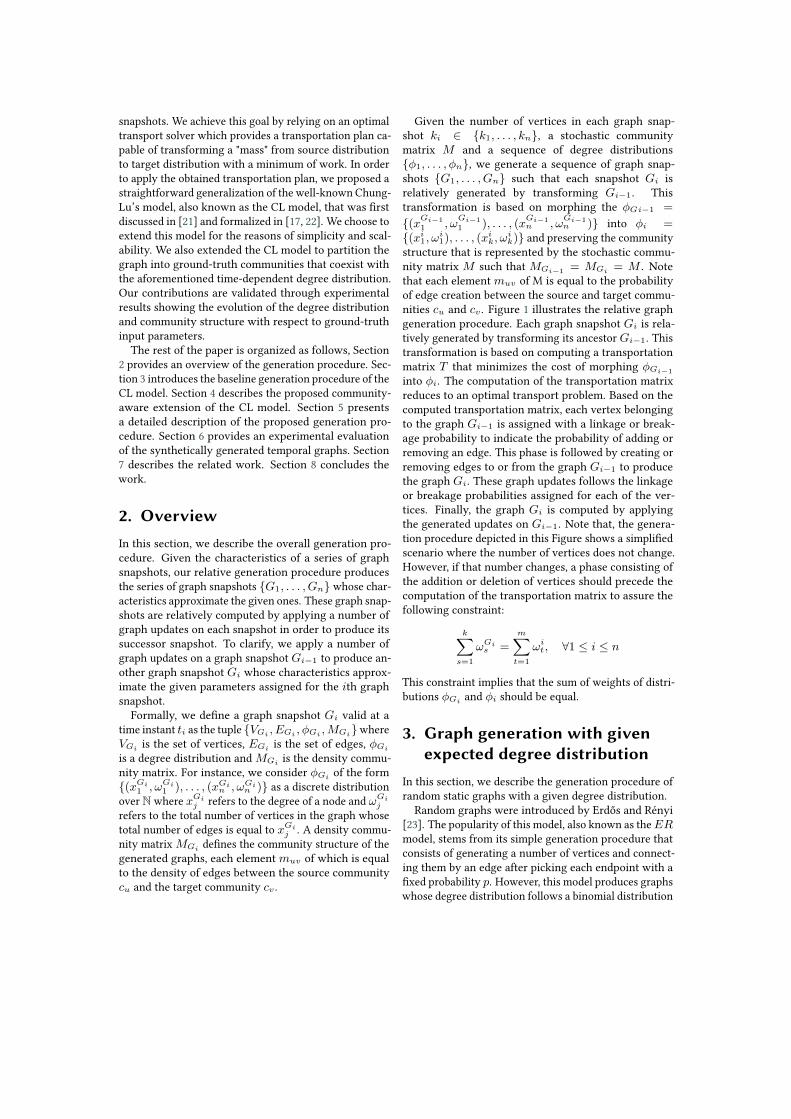
structure that is represented by the stochastic commu-nity matrix 𝑀 such that 𝑀𝐺𝑖−1 = 𝑀𝐺𝑖 = 𝑀 . Notethat each element 𝑚𝑢𝑣 of M is equal to the probabilityof edge creation between the source and target commu-nities 𝑐𝑢 and 𝑐𝑣 . Figure 1 illustrates the relative graphgeneration procedure. Each graph snapshot 𝐺𝑖 is rela-tively generated by transforming its ancestor 𝐺𝑖−1. Thistransformation is based on computing a transportationmatrix 𝑇 that minimizes the cost of morphing 𝜑𝐺𝑖−1

into 𝜑𝑖. The computation of the transportation matrixreduces to an optimal transport problem. Based on thecomputed transportation matrix, each vertex belongingto the graph 𝐺𝑖−1 is assigned with a linkage or break-age probability to indicate the probability of adding orremoving an edge. This phase is followed by creating orremoving edges to or from the graph 𝐺𝑖−1 to producethe graph 𝐺𝑖. These graph updates follows the linkageor breakage probabilities assigned for each of the ver-tices. Finally, the graph 𝐺𝑖 is computed by applyingthe generated updates on 𝐺𝑖−1. Note that, the genera-tion procedure depicted in this Figure shows a simplifiedscenario where the number of vertices does not change.However, if that number changes, a phase consisting ofthe addition or deletion of vertices should precede thecomputation of the transportation matrix to assure thefollowing constraint:

𝑘∑︁𝑠=1

𝜔𝐺𝑖𝑠 =

𝑚∑︁𝑡=1

𝜔𝑖𝑡, ∀1 ≤ 𝑖 ≤ 𝑛

This constraint implies that the sum of weights of distri-butions 𝜑𝐺𝑖 and 𝜑𝑖 should be equal.

3. Graph generation with givenexpected degree distribution

In this section, we describe the generation procedure ofrandom static graphs with a given degree distribution.

Random graphs were introduced by Erdős and Rényi[23]. The popularity of this model, also known as the 𝐸𝑅model, stems from its simple generation procedure thatconsists of generating a number of vertices and connect-ing them by an edge after picking each endpoint with afixed probability 𝑝. However, this model produces graphswhose degree distribution follows a binomial distribution

Figure 1: Relative graph generation procedure.

with a mean degree equals to (𝑁−1)𝑝 where 𝑁 is the to-tal number of vertices. Hence, it fails to mimic real-worldgraphs that usually follow a power-law degree distribu-tion. To tackle this limitation, the edge configurationmodel [24] consists of generating a random graph whosedegree distribution matches, approximately, a given de-gree distribution. That is, each vertex is assigned with anumber of stubs equal to its desired degree that is drawnindependently from the given degree distribution. Hav-ing this, pairs of stubs are linked randomly forming edgesbetween their endpoints. Although this technique ap-proximately matches any given degree distribution, arelaxed version known as the Chung-Lu model was in-troduced in [21]. This model consists of generating a ran-dom graph that approximately matches a given degreedistribution relying on a simple generation procedurethat can be considered as a variant of the 𝐸𝑅 model. Forsimplicity, we will refer to this model as the CL model inthe following description.

Consider the degree distribution 𝜑 as the input param-eter to the CL model and the undirected, unweighted andunlabeled graph 𝐺 = {𝑉,𝐸, 𝜑𝐺} as the output where𝜑𝐺 denotes the degree distribution of 𝐺, 𝑉 and 𝐸 de-note the set of vertices and edges, respectively. Havingthis, the CL model produces a graph 𝐺 such that 𝜑𝐺 isan approximation of 𝜑. The main idea is to pick eachendpoint of an edge with a certain probability such that,at the end of the generation procedure, the total numberof incident edges to each vertex is close to its assigneddegree. Hence, the starting phase consists of assigningeach vertex 𝑣𝑖 ∈ 𝑉 with a degree 𝑑𝑣𝑖 and a linkageprobability 𝑝𝑣𝑖 ∝ 𝑑𝑣𝑖 . Considering that 𝐷 is the sum ofthe degrees extracted from 𝜑, we define the CL linkage

probability 𝑝𝑣𝑖 in the following Equation:

𝑝𝑣𝑖 =𝑑𝑣𝑖𝐷

(1)

Subsequently, a linkage phase consists of picking |𝐸| =𝐷2

pairs of vertices to connect such that for a sufficientlylarge |𝐸| the random variable denoting the degree ofvertex 𝑣𝑖 is Poisson distributed with a mean equals to𝑑𝑣𝑖 . Iterating the linkage phase |𝐸| times where an edgeis equally likely to be chosen in both directions for undi-rected graphs, the insertion probability of an edge con-necting vertex 𝑣𝑖 and vertex 𝑣𝑗 is 𝑝𝑣𝑖𝑣𝑗 = 2𝑝𝑣𝑖𝑝𝑣𝑗

𝐷2

.The edge insertion probability can be rewritten in themore convenient form:

𝑝𝑣𝑖𝑣𝑗 =𝑑𝑣𝑖𝑑𝑣𝑗𝐷

For optimisation sake, we gather all vertices shar-ing the same degree together in a pool 𝛾𝑑 ={𝑣𝑖|𝑣𝑖 ∈ 𝑉 ∧ 𝑑𝑣𝑖 = 𝑑} that we use as a subsidiary gen-eration component. Each vertex in a pool is equally likelyto be chosen assuring that the aforementioned linkageprobability 𝑝𝑣𝑖 is not affected for a sufficiently large num-ber of vertices. After the degree assignment phase, ver-tices are distributed throughout the pools having eachthe following linkage probability:

𝑝𝛾𝑑 =𝑑|𝛾𝑑|𝐷

Now, instead of picking vertices a pool is first pickedIt should be highlighted that self-loops or multi-edgescan be created since each endpoint of an edge is pickedindependently. The number of these edges, however, isindependent of the number of vertices and thus can beneglected for large scale graphs.

4. Community-aware graphgeneration with given expecteddegree distribution

Although the CL model produces graphs with respectto a given degree distribution, it is not aware of thecommunity structure existing in most real-world graphs.Hence, we propose a community-aware extension of theCL model based on the stochastic block model (SBM).Since a community is not quantitatively well defined,many definitions where provided in literature. Intuitively,one can consider a community as a subgraph which ver-tices are more densely connected between each otherthan they are with the rest of the graph. Let’s considerthe set of communities 𝐶 = {𝑐𝑖} and suppose that a ver-tex should belong to one community and edges shouldbe differentiated into within and between edges:

• Given a community 𝑐𝑖, an edge 𝑒 is called a withinedge if the source vertex∈ 𝑐𝑖 and the target vertex∈ 𝑐𝑖.

• Given two communities 𝑐𝑖 and 𝑐𝑗 , an edge 𝑒 iscalled a between edge if the source vertex ∈ 𝑐𝑖and target vertex ∈ 𝑐𝑗 or vice versa.

To insure that vertices belonging to a community aremore densely connected to each other than they are withthe rest of the graph, the within and between edge cre-ation probabilities 𝑝𝑖𝑛𝑐𝑖 and 𝑝𝑜𝑢𝑡𝑐𝑖 of 𝑐𝑖 must satisfy thecondition 𝑝𝑖𝑛𝑐𝑖 > 𝑝𝑜𝑢𝑡𝑐𝑖 , ∀𝑐𝑖 ∈ 𝐶 .

4.1. Stochastic block modelIn this section, we formulate the SBM model [9] (alsoknown as the planted partition model) which is com-monly used for the generation of random graphs with agiven community structure. Hence, this generation pro-cedure only considers controlling the community struc-ture of the graph and overlooks the resulting degree dis-tribution. The input of the generation procedure is astochastic community matrix 𝑀 , each element 𝑚𝑖𝑗 ofwhich defines the probability of edge creation betweenthe source community 𝑐𝑖 and the target community 𝑐𝑗 .The output is a graph 𝐺 = {𝑉,𝐸,𝑀𝐺} where 𝑀𝐺 isthe obtained density community matrix, each element𝑚𝐺

𝑖𝑗 of which defines the relative edge density betweenthe source community 𝑐𝑖 and the target community 𝑐𝑗 .The generation procedure starts with the distribution ofvertices between the planted communities such that eachvertex belongs to a single community. Now, the linkageprobability between a vertex belonging to community 𝑐𝑖and another vertex belonging to community 𝑐𝑗 is equal to𝑚𝑖𝑗 . However, the extracted community density matrix𝑀𝐺 from the resulting graph 𝐺 is an approximation of𝑀 . That is, each element 𝑚𝐺𝑖𝑗 is binomially distributedwith mean equals to 𝑚𝑖𝑗 and Poisson distributed withthe same mean for a sufficiently large number of edges.

4.2. Stochastic block model with givendegree distribution

In this section, we propose a static graph generationprocedure which controls both the community structureand degree distribution. Given a degree distribution 𝜑and a stochastic community matrix 𝑀 , our proposedmodel generates a graph 𝐺 which degree distribution 𝜑𝐺

is an approximation of 𝜑 and density community matrix𝑀𝑔 is an approximation of 𝑀 . In the following, weprovide a description of our generation mechanism thatextends the stochastic block model depicted in Section4.1.

Since the generated graph 𝐺 is undirected, the matrix𝑀 is symmetric such that 𝑚𝑖𝑗 = 𝑚𝑗𝑖. Having this, we

define 𝜔𝑖𝑗 = 𝜔𝑗𝑖 = 2𝑚𝑖𝑗 and 𝜔𝑖𝑖 = 𝑚𝑖𝑖. Furthermore,we assign each community 𝑐𝑖 with a within edge creationprobability 𝑝𝑖𝑛𝑐𝑖 , a between edge creation equal to 𝑝𝑜𝑢𝑡𝑐𝑖

and a probability of edge creation 𝑝𝑐𝑖 such that:

𝑝𝑐𝑖 = 𝑝𝑖𝑛𝑐𝑖 + 𝑝𝑜𝑢𝑡𝑐𝑖 = 𝜔𝑖𝑖 + 0.5

|𝐶|∑︁𝑗=1,𝑗 ̸=𝑖

𝜔𝑖𝑗 (2)

We define the linkage probability 𝑝𝑣𝑖 of choosing a vertex𝑣𝑖 belonging to community 𝑐𝑚 as follows:

𝑝𝑣𝑖 =𝑑𝑣𝑖𝐷𝑐𝑚

𝑝𝑐𝑚 , 𝑣𝑖 ∈ 𝑐𝑚 (3)

where 𝐷𝑐𝑚 is the sum of the degrees of vertices belong-ing to community 𝑐𝑚 and 𝑝𝑐𝑚 is the probability of choos-ing 𝑐𝑚. The linkage probability of a vertex is the productof the probability 𝑝𝑐𝑚 of choosing the community towhich the vertex belongs and the probability

𝑑𝑣𝑖𝐷𝑐𝑚

ofchoosing the vertex 𝑣𝑖 in that community. Hence, Equa-tion 3 assures the approximation of the community ma-trix. However, 𝑝𝑣𝑖 should be equal to

𝑑𝑣𝑖𝐷

(Equation 1)to assure the approximation of the degree distribution.Therefore, we define the following condition in order toreduce Equation (3) to Equation (1):

𝐷𝑐𝑚 = 𝐷𝑝𝑐𝑚

Now, replacing 𝐷 by 𝐷𝑐𝑚𝐷𝑝𝑐𝑚

in the original CL linkageprobability (Equation 1) which assures the control of thedegree distribution, we obtain Equation 3 which assuresthe control of the community structure. Having this, theduality of the linkage probability given in Equations (1)and (3) insures that both requirements are satisfied byour generation procedure.

For performance amelioration, we consider the selec-tion of pools rather than vertices such that a pool is localto one community. That is vertices having the same de-gree variation and belonging to the same community 𝑐𝑚are grouped in a pool 𝛾𝑐𝑚

𝑑 = {𝑣𝑖|𝑣𝑖 ∈ 𝑐𝑚 ∧ 𝑑𝑣𝑖 = 𝑑}such that the probability of a pool selection for edgeinsertion is:

𝑝𝛾𝑐𝑚𝑑

=𝑑|𝛾𝑐𝑚

𝑑 |𝐷

4.3. Hierarchical community structureThe specification of the stochastic matrix is not straight-forward and imposes an exhaustive number of user-defined parameters. Hence, we define an auto-generativeprocedure that fills the matrix with no exogenous effort.Considering a static graph, we construct a stochastic ma-trix that reflects a hierarchical community structure withonly two given parameters. In a hierarchical communitymatrix, communities recursively embed subsequent com-munities in a self-similar fashion such that the commu-nity structure is represented by a hierarchical tree where

each node represents a community. Each non-leaf nodeis expanded into 𝑏 other nodes until reaching a desiredtree height ℎ (Figure 2). The ending recursion results in𝑛𝑐 = 𝑏ℎ leaf-nodes referencing the finest scale communi-ties having a linkage probability 𝜔𝑖𝑗 proportional to thedistance between 𝑐𝑖 and 𝑐𝑗 . The distance between twocommunities, 𝑑(𝑐𝑖, 𝑐𝑗), is equal to the number of hopstraversed in order to reach the least common ancestor ofthese communities. In order to satisfy the condition stat-ing that within edge linkage probability must be higherthan between linkage probability (𝑝𝑖𝑛𝑐𝑖 > 𝑝𝑜𝑢𝑡𝑐𝑖 ), we define𝜔𝑖𝑖 as follows:

𝜔𝑖𝑖 = 0.5

𝑛𝑐−1∑︁𝑗=0,𝑗 ̸=𝑖

𝜔𝑖𝑗 + 𝑘

where 𝑘 is a tunable parameter which calibration steersthe difference between within and between edge densi-ties. The effect of varying 𝑘 is further highlighted in theSection 6.

Figure 2: Hierarchical community tree with height ℎ andbranching factor 𝑏.

5. Relative graph generationIn order to control the evolution of the degree distribu-tion of the generated temporal graphs, we propose in thissection an extension of the CL model that is based on theoptimal transport to compute the minimal distance be-tween the degree distributions of each pair of successivegraph snapshots.

5.1. Earth mover’s distanceThe Earth mover’s distance can be defined as a mea-sure of distance over a domain 𝐷 between two dis-tributions of the form {(𝑥1, 𝜔1), ..., (𝑥𝑛, 𝜔𝑛)} where𝑥𝑖 ∈ 𝐷 and 𝜔𝑖 is the density of 𝑥𝑖. Having this,the problem reduces to the computation of an optimalflow (transportation matrix) 𝑇 = [𝑡𝑖𝑗 ] between twodistributions 𝑃 = {(𝑥1, 𝑝1), ..., (𝑥𝑛, 𝑝𝑛)} and 𝑄 ={(𝑦1, 𝑞1), ..., (𝑦𝑛, 𝑞𝑛)} such that 𝑡𝑖𝑗 is the mass trans-ported between 𝑝𝑖 and 𝑞𝑗 which minimizes the overall

cost:

min𝑇

𝑛∑︁𝑖=1

𝑚∑︁𝑗=1

𝑡𝑖𝑗𝑑𝑖𝑗

where 𝑑𝑖𝑗 = 𝑑(𝑥𝑖, 𝑦𝑗) is a measure of distance between𝑥𝑖 and 𝑦𝑗 . The following constraints must hold for theoptimal flow 𝑇 :

𝑡𝑖𝑗 ≥ 0, 1 ≥ 𝑖 ≥ 𝑛, 1 ≥ 𝑗 ≥ 𝑚

𝑚∑︁𝑗=1

𝑡𝑖𝑗 ≤ 𝑝𝑖, 1 ≥ 𝑖 ≥ 𝑛,

𝑛∑︁𝑖=1

𝑡𝑖𝑗 ≤ 𝑞𝑗 , 1 ≥ 𝑗 ≥ 𝑚

Once the optimal flow 𝑇 is found, the EMD between𝑃 and 𝑄 is computed as follows:

𝐸𝑀𝐷(𝑃,𝑄) =

∑︀𝑛𝑖=1

∑︀𝑚𝑗=1 𝑡𝑖𝑗𝑑𝑖𝑗∑︀𝑛

𝑖=1

∑︀𝑚𝑗=1 𝑡𝑖𝑗

The EMD is fundamental in our generation proceduresince it is used to compute the distance between twodegree distributions as described in the following Section.

5.2. Baseline relative graph generationIn this section, we provide the baseline procedure oftransforming a graph 𝐺 with degree distribution 𝜑 into𝐺′ with degree distribution 𝜑′ which we refer to as theBaseline relative graph generation. Note that, we use thistechnique for generating temporal graphs such that 𝐺and 𝐺′ corresponds to successive graph snapshots. Forgeneralisation purposes, however, we remove the notionof time in this section. This transformation is enabled by aset of atomic graph operations including the addition anddeletion of a vertex or an edge. Following the assumptionthat temporal graphs gradually evolve, this number ofgraph operations between successive snapshots shouldbe minimized which is assured in our model by applyingan optimal transport method.

Consider the input graph 𝐺 = {𝑉,𝐸, 𝜑} and de-gree distribution 𝜑′, the generated output graph 𝐺′ ={𝑉 ′, 𝐸′, 𝜑𝐺′} such that 𝜑𝐺′ is an approximation of 𝜑′.We define the distance between two degree distributions𝜑 and 𝜑′ as the earth mover’s distance 𝐸𝑀𝐷(𝜑, 𝜑′).

Consider 𝛿𝑛 = |𝑉 ′| − |𝑉 | as the total number of ver-tices to be added to or removed from the graph basedon whether 𝛿𝑛 is a positive or negative number, respec-tively. When adding a new vertex, this vertex is assignedwith a degree equals to 0 and deleting a vertex consistsof removing the vertex with its corresponding incidentedges. This transformation phase assures that 𝐺 and 𝐺′

share the same number of vertices, hence, enables thetransformation of 𝜑 into 𝜑′. In order to morph 𝜑 into𝜑′, a transportation matrix 𝑇 is computed, where eachrow corresponds to a degree 𝑑 in the set of degrees in thesource distribution 𝜑 and each column corresponds to a

degree 𝑑′ in the set of degrees in the target distribution 𝜑′.Now, each cell consists of the portion of vertices havinga degree 𝑑 for which links are to be inserted or removedin order to be assigned a total number of edges equals todegree 𝑑′. That is, a vertex 𝑣𝑖, with a degree 𝑑𝑣𝑖 = 𝑑, willbe assigned a degree variation of 𝛿𝑑𝑣𝑖 = 𝑑′−𝑑 resultingin a total number of edge insertions and deletions definedas 𝐷+ and 𝐷−, respectively.We assign, for each vertex 𝑣𝑖, a linkage probability 𝑝+𝑣𝑖 ora breakage probability 𝑝−𝑣𝑖 defined as extensions of theCL linkage probability (1):

𝑝+𝑣𝑖 =𝛿𝑑𝑣𝑖𝐷+

, 𝛿𝑑𝑣𝑖 > 0 (4)

𝑝−𝑣𝑖 =−𝛿𝑑𝑣𝑖𝐷− , 𝛿𝑑𝑣𝑖 < 0 (5)

We collect vertices sharing the same degree variation𝛿𝑑 = 𝑑′ − 𝑑 into a linkage pool if 𝛿𝑑 > 0 and in abreakage pool if 𝛿𝑑 < 0. Consider 𝛾𝑑→𝑑′ = {𝑣𝑖|𝑣𝑖 ∈𝑉 ∧ 𝛿𝑣𝑖 = 𝑑′ − 𝑑} to be the pool containing verticeshaving a degree 𝑑 that should be transformed into 𝑑′. Wecompute the probability of picking a linkage or breakagepool 𝑝+𝛾𝑑→𝑑′

and 𝑝−𝛾𝑑→𝑑′as follows:

𝑝+𝛾𝑑→𝑑′=

𝛿𝑑|𝛾𝑑→𝑑′ |𝐷+

, 𝛿𝑑 > 0

𝑝−𝛾𝑑→𝑑′=−𝛿𝑑|𝛾𝑑→𝑑′ |

𝐷− , 𝛿𝑑 < 0

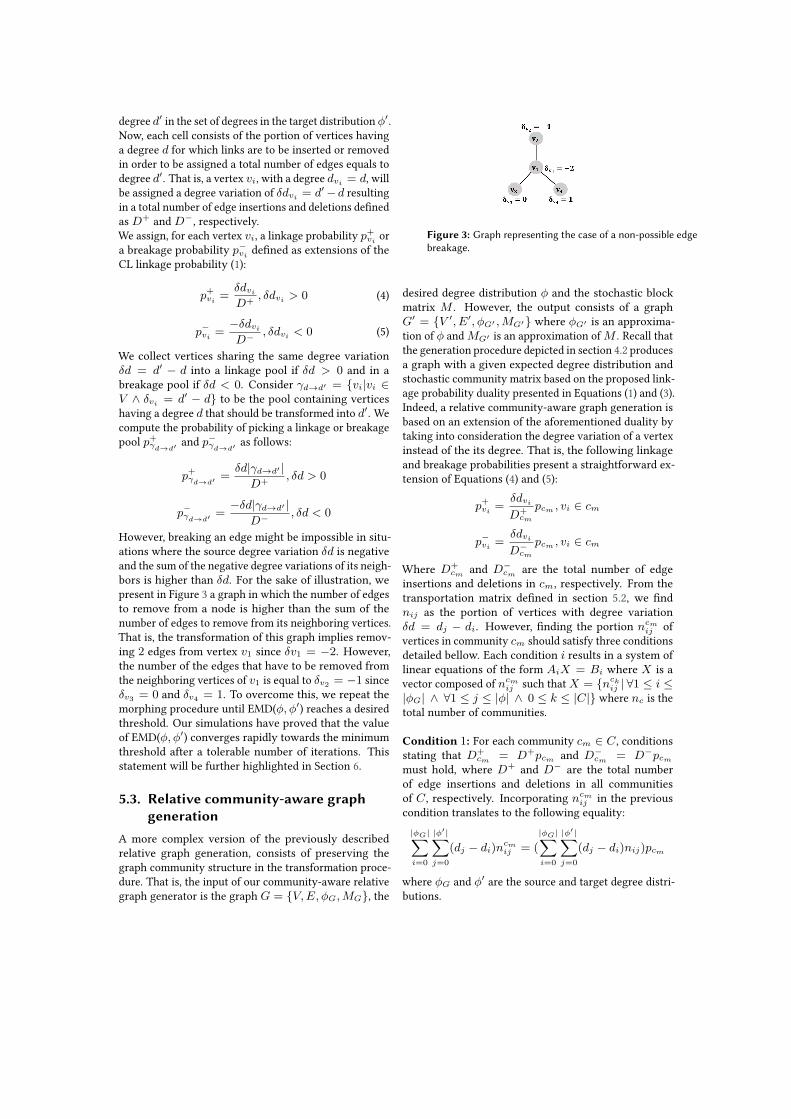
However, breaking an edge might be impossible in situ-ations where the source degree variation 𝛿𝑑 is negativeand the sum of the negative degree variations of its neigh-bors is higher than 𝛿𝑑. For the sake of illustration, wepresent in Figure 3 a graph in which the number of edgesto remove from a node is higher than the sum of thenumber of edges to remove from its neighboring vertices.That is, the transformation of this graph implies remov-ing 2 edges from vertex 𝑣1 since 𝛿𝑣1 = −2. However,the number of the edges that have to be removed fromthe neighboring vertices of 𝑣1 is equal to 𝛿𝑣2 = −1 since𝛿𝑣3 = 0 and 𝛿𝑣4 = 1. To overcome this, we repeat themorphing procedure until EMD(𝜑, 𝜑′) reaches a desiredthreshold. Our simulations have proved that the valueof EMD(𝜑, 𝜑′) converges rapidly towards the minimumthreshold after a tolerable number of iterations. Thisstatement will be further highlighted in Section 6.

5.3. Relative community-aware graphgeneration

A more complex version of the previously describedrelative graph generation, consists of preserving thegraph community structure in the transformation proce-dure. That is, the input of our community-aware relativegraph generator is the graph 𝐺 = {𝑉,𝐸, 𝜑𝐺,𝑀𝐺}, the

Figure 3: Graph representing the case of a non-possible edgebreakage.

desired degree distribution 𝜑 and the stochastic blockmatrix 𝑀 . However, the output consists of a graph𝐺′ = {𝑉 ′, 𝐸′, 𝜑𝐺′ ,𝑀𝐺′} where 𝜑𝐺′ is an approxima-tion of 𝜑 and 𝑀𝐺′ is an approximation of 𝑀 . Recall thatthe generation procedure depicted in section 4.2 producesa graph with a given expected degree distribution andstochastic community matrix based on the proposed link-age probability duality presented in Equations (1) and (3).Indeed, a relative community-aware graph generation isbased on an extension of the aforementioned duality bytaking into consideration the degree variation of a vertexinstead of the its degree. That is, the following linkageand breakage probabilities present a straightforward ex-tension of Equations (4) and (5):

𝑝+𝑣𝑖 =𝛿𝑑𝑣𝑖𝐷+

𝑐𝑚

𝑝𝑐𝑚 , 𝑣𝑖 ∈ 𝑐𝑚

𝑝−𝑣𝑖 =𝛿𝑑𝑣𝑖𝐷−

𝑐𝑚

𝑝𝑐𝑚 , 𝑣𝑖 ∈ 𝑐𝑚

Where 𝐷+𝑐𝑚 and 𝐷−

𝑐𝑚 are the total number of edgeinsertions and deletions in 𝑐𝑚, respectively. From thetransportation matrix defined in section 5.2, we find𝑛𝑖𝑗 as the portion of vertices with degree variation𝛿𝑑 = 𝑑𝑗 − 𝑑𝑖. However, finding the portion 𝑛𝑐𝑚

𝑖𝑗 ofvertices in community 𝑐𝑚 should satisfy three conditionsdetailed bellow. Each condition 𝑖 results in a system oflinear equations of the form 𝐴𝑖𝑋 = 𝐵𝑖 where 𝑋 is avector composed of 𝑛𝑐𝑚

𝑖𝑗 such that 𝑋 = {𝑛𝑐𝑘𝑖𝑗 | ∀1 ≤ 𝑖 ≤

|𝜑𝐺| ∧ ∀1 ≤ 𝑗 ≤ |𝜑| ∧ 0 ≤ 𝑘 ≤ |𝐶|} where 𝑛𝑐 is thetotal number of communities.

Condition 1: For each community 𝑐𝑚 ∈ 𝐶 , conditionsstating that 𝐷+

𝑐𝑚 = 𝐷+𝑝𝑐𝑚 and 𝐷−𝑐𝑚 = 𝐷−𝑝𝑐𝑚

must hold, where 𝐷+ and 𝐷− are the total numberof edge insertions and deletions in all communitiesof 𝐶 , respectively. Incorporating 𝑛𝑐𝑚

𝑖𝑗 in the previouscondition translates to the following equality:

|𝜑𝐺|∑︁𝑖=0

|𝜑′|∑︁𝑗=0

(𝑑𝑗 − 𝑑𝑖)𝑛𝑐𝑚𝑖𝑗 = (

|𝜑𝐺|∑︁𝑖=0

|𝜑′|∑︁𝑗=0

(𝑑𝑗 − 𝑑𝑖)𝑛𝑖𝑗)𝑝𝑐𝑚

where 𝜑𝐺 and 𝜑′ are the source and target degree distri-butions.

Condition 2: This condition states that the sum ofall portions of vertices with degree variation 𝑑𝑗 − 𝑑𝑖∀𝑑𝑗 ∈ 𝜑𝑡 in 𝑐𝑚 should be equal to the portion 𝑛𝑐𝑚

𝑖 ofvertices in 𝑐𝑚 having a degree 𝑑𝑖 resulting in the follow-ing equality:

𝑚∑︁𝑗=0

𝑛𝑐𝑚𝑖𝑗 = 𝑛𝑐𝑚

𝑖

Condition 3: This condition states that the por-tion 𝑛𝑖𝑗 of vertices with degree variation 𝑑𝑗 − 𝑑𝑖 inthe graph must be equal to the sum of all portions 𝑛𝑐𝑚

𝑖𝑗

∀𝑐𝑚 ∈ 𝐶.𝑛𝑐∑︁

𝑐𝑚=0

𝑛𝑐𝑚𝑖𝑗 = 𝑛𝑖𝑗

By solving the concatenated system of equations obtainedfrom the previous conditions 𝑐𝑜𝑛𝑐𝑎𝑡(𝐴1, 𝐴2, 𝐴3)𝑋 =𝑐𝑜𝑛𝑐𝑎𝑡(𝐵1, 𝐵2, 𝐵3), we find the vector 𝑋 , hence thevalues of 𝑛𝑐𝑚

𝑖𝑗 . Pools are created on a local basis in eachcommunity such that vertices with the same degree vari-ation 𝛿𝑑 = 𝑑′− 𝑑 and belonging to the same community𝑐𝑚 are collected in a single pool 𝛾𝑐𝑚

𝑑→𝑑′ . We computethe probability of picking a linkage or breakage pool𝑝+𝛾𝑑→𝑑′ ,𝑐𝑚

and 𝑝−𝛾𝑑→𝑑′ ,𝑐𝑚as follows:

𝑝+𝛾𝑑→𝑑′ ,𝑐𝑚=

𝛿𝑑|𝛾𝑐𝑚𝑑→𝑑′ |

𝐷+, 𝛿𝑑 > 0

𝑝−𝛾𝑑→𝑑′ ,𝑐𝑚=−𝛿𝑑|𝛾𝑐𝑚

𝑑→𝑑′ |𝐷− , 𝛿𝑑 < 0

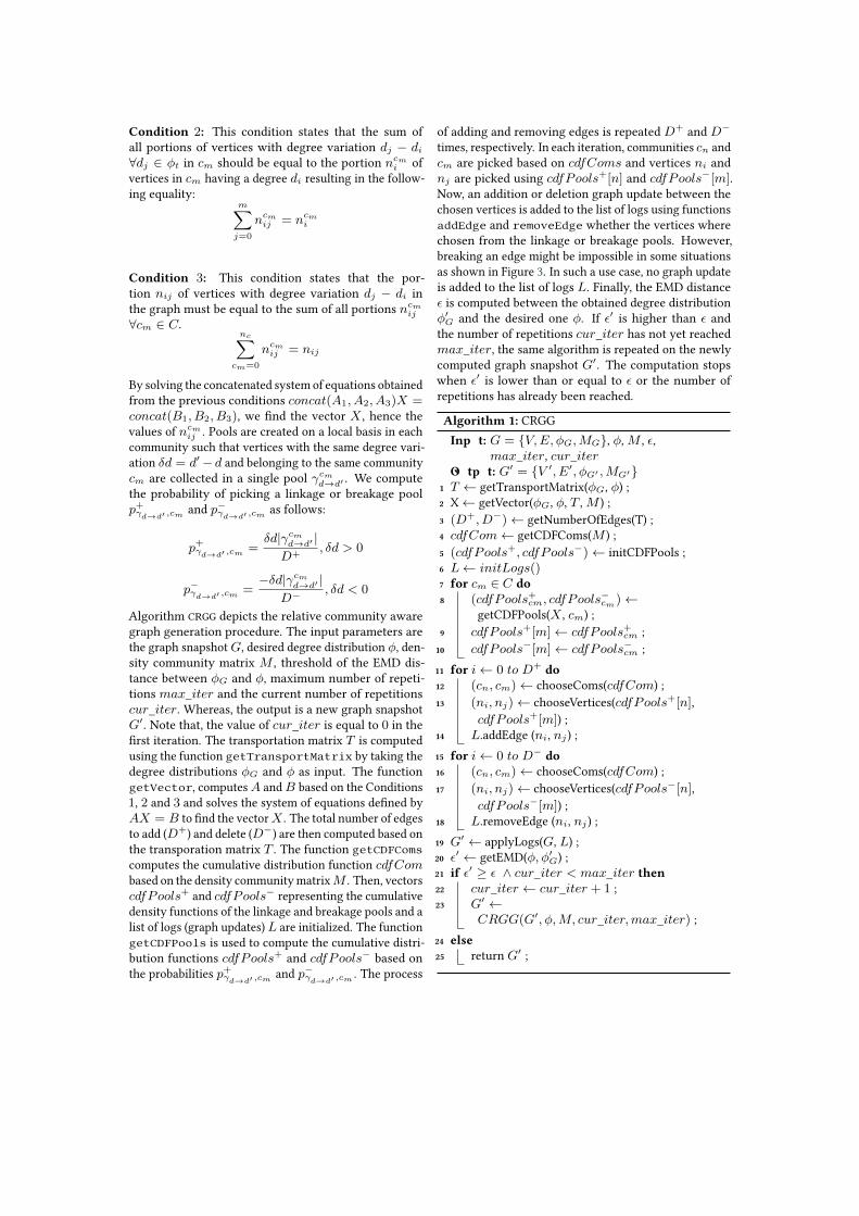
Algorithm CRGG depicts the relative community awaregraph generation procedure. The input parameters arethe graph snapshot 𝐺, desired degree distribution 𝜑, den-sity community matrix 𝑀 , threshold of the EMD dis-tance between 𝜑𝐺 and 𝜑, maximum number of repeti-tions 𝑚𝑎𝑥_𝑖𝑡𝑒𝑟 and the current number of repetitions𝑐𝑢𝑟_𝑖𝑡𝑒𝑟. Whereas, the output is a new graph snapshot𝐺′. Note that, the value of 𝑐𝑢𝑟_𝑖𝑡𝑒𝑟 is equal to 0 in thefirst iteration. The transportation matrix 𝑇 is computedusing the function getTransportMatrix by taking thedegree distributions 𝜑𝐺 and 𝜑 as input. The functiongetVector, computes 𝐴 and 𝐵 based on the Conditions1, 2 and 3 and solves the system of equations defined by𝐴𝑋 = 𝐵 to find the vector𝑋 . The total number of edgesto add (𝐷+) and delete (𝐷−) are then computed based onthe transporation matrix 𝑇 . The function getCDFComscomputes the cumulative distribution function 𝑐𝑑𝑓𝐶𝑜𝑚based on the density community matrix𝑀 . Then, vectors𝑐𝑑𝑓𝑃𝑜𝑜𝑙𝑠+ and 𝑐𝑑𝑓𝑃𝑜𝑜𝑙𝑠− representing the cumulativedensity functions of the linkage and breakage pools and alist of logs (graph updates) 𝐿 are initialized. The functiongetCDFPools is used to compute the cumulative distri-bution functions 𝑐𝑑𝑓𝑃𝑜𝑜𝑙𝑠+ and 𝑐𝑑𝑓𝑃𝑜𝑜𝑙𝑠− based onthe probabilities 𝑝+𝛾𝑑→𝑑′ ,𝑐𝑚

and 𝑝−𝛾𝑑→𝑑′ ,𝑐𝑚. The process

of adding and removing edges is repeated 𝐷+ and 𝐷−

times, respectively. In each iteration, communities 𝑐𝑛 and𝑐𝑚 are picked based on 𝑐𝑑𝑓𝐶𝑜𝑚𝑠 and vertices 𝑛𝑖 and𝑛𝑗 are picked using 𝑐𝑑𝑓𝑃𝑜𝑜𝑙𝑠+[𝑛] and 𝑐𝑑𝑓𝑃𝑜𝑜𝑙𝑠−[𝑚].Now, an addition or deletion graph update between thechosen vertices is added to the list of logs using functionsaddEdge and removeEdge whether the vertices wherechosen from the linkage or breakage pools. However,breaking an edge might be impossible in some situationsas shown in Figure 3. In such a use case, no graph updateis added to the list of logs 𝐿. Finally, the EMD distance𝜖 is computed between the obtained degree distribution𝜑′𝐺 and the desired one 𝜑. If 𝜖′ is higher than 𝜖 and

the number of repetitions 𝑐𝑢𝑟_𝑖𝑡𝑒𝑟 has not yet reached𝑚𝑎𝑥_𝑖𝑡𝑒𝑟, the same algorithm is repeated on the newlycomputed graph snapshot 𝐺′. The computation stopswhen 𝜖′ is lower than or equal to 𝜖 or the number ofrepetitions has already been reached.

Algorithm 1: CRGG

Input: 𝐺 = {𝑉,𝐸, 𝜑𝐺,𝑀𝐺}, 𝜑, 𝑀 , 𝜖,𝑚𝑎𝑥_𝑖𝑡𝑒𝑟, 𝑐𝑢𝑟_𝑖𝑡𝑒𝑟

Output: 𝐺′ = {𝑉 ′, 𝐸′, 𝜑𝐺′ ,𝑀𝐺′}1 𝑇 ← getTransportMatrix(𝜑𝐺, 𝜑) ;2 X← getVector(𝜑𝐺, 𝜑, 𝑇 , 𝑀 ) ;3 (𝐷+, 𝐷−)← getNumberOfEdges(T) ;4 𝑐𝑑𝑓𝐶𝑜𝑚← getCDFComs(𝑀 ) ;5 (𝑐𝑑𝑓𝑃𝑜𝑜𝑙𝑠+, 𝑐𝑑𝑓𝑃𝑜𝑜𝑙𝑠−)← initCDFPools ;6 𝐿← 𝑖𝑛𝑖𝑡𝐿𝑜𝑔𝑠()7 for 𝑐𝑚 ∈ 𝐶 do8 (𝑐𝑑𝑓𝑃𝑜𝑜𝑙𝑠+𝑐𝑚, 𝑐𝑑𝑓𝑃𝑜𝑜𝑙𝑠−𝑐𝑚)←

getCDFPools(𝑋 , 𝑐𝑚) ;9 𝑐𝑑𝑓𝑃𝑜𝑜𝑙𝑠+[𝑚]← 𝑐𝑑𝑓𝑃𝑜𝑜𝑙𝑠+𝑐𝑚 ;

10 𝑐𝑑𝑓𝑃𝑜𝑜𝑙𝑠−[𝑚]← 𝑐𝑑𝑓𝑃𝑜𝑜𝑙𝑠−𝑐𝑚 ;

11 for 𝑖← 0 𝑡𝑜 𝐷+ do12 (𝑐𝑛, 𝑐𝑚)← chooseComs(𝑐𝑑𝑓𝐶𝑜𝑚) ;13 (𝑛𝑖, 𝑛𝑗)← chooseVertices(𝑐𝑑𝑓𝑃𝑜𝑜𝑙𝑠+[𝑛],

𝑐𝑑𝑓𝑃𝑜𝑜𝑙𝑠+[𝑚]) ;14 𝐿.addEdge (𝑛𝑖, 𝑛𝑗 ) ;

15 for 𝑖← 0 𝑡𝑜 𝐷− do16 (𝑐𝑛, 𝑐𝑚)← chooseComs(𝑐𝑑𝑓𝐶𝑜𝑚) ;17 (𝑛𝑖, 𝑛𝑗)← chooseVertices(𝑐𝑑𝑓𝑃𝑜𝑜𝑙𝑠−[𝑛],

𝑐𝑑𝑓𝑃𝑜𝑜𝑙𝑠−[𝑚]) ;18 𝐿.removeEdge (𝑛𝑖, 𝑛𝑗 ) ;

19 𝐺′ ← applyLogs(𝐺, 𝐿) ;20 𝜖′ ← getEMD(𝜑, 𝜑′

𝐺) ;21 if 𝜖′ ≥ 𝜖 ∧ 𝑐𝑢𝑟_𝑖𝑡𝑒𝑟 < 𝑚𝑎𝑥_𝑖𝑡𝑒𝑟 then22 𝑐𝑢𝑟_𝑖𝑡𝑒𝑟 ← 𝑐𝑢𝑟_𝑖𝑡𝑒𝑟 + 1 ;23 𝐺′ ←

𝐶𝑅𝐺𝐺(𝐺′, 𝜑,𝑀, 𝑐𝑢𝑟_𝑖𝑡𝑒𝑟,𝑚𝑎𝑥_𝑖𝑡𝑒𝑟) ;

24 else25 return 𝐺′ ;

10

8

Timest

amp

6

4

2

0100

80

60

Degree

40

15000

10000

5000

0

20

Number of occurrences

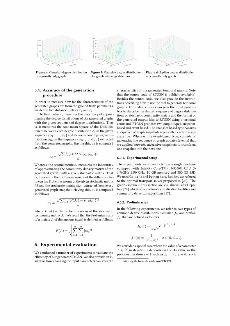
Figure 4: Gaussian degree distributionof a growth only graph

10

8

Timest

amp

6

4

2

0100

80

60

Degree

40

0

4

2

10

8

6

20

×104

Number of occurrences

Figure 5: Gaussian degree distributionof a graph with edge deletions

10

8

Timest

amp

6

4

2

060

40Degree

20

6

4

3

5

1

0

2

0

×104

Number of occurrences

Figure 6: Zipfian degree distributionof a growth only graph

5.4. Accuracy of the generationprocedure

In order to measure how far the characteristics of thegenerated graphs are from the ground truth parameters,we define two distance metrics 𝜀𝑑 and 𝜀𝑐.

The first metric 𝜀𝑑 measures the inaccuracy of approx-imating the degree distributions of the generated graphswith the given sequence of degree distributions. Thatis, it measures the root mean square of the EMD dis-tances between each degree distribution 𝜑𝑖 in the givensequence {𝜑1, . . . , 𝜑𝑛} and its corresponding degree dis-tribution 𝜑𝐺𝑖 in the sequence {𝜑𝐺1 , . . . 𝜑𝐺𝑛} extractedfrom the generated graphs. Having this, 𝜀𝑑 is computedas follows:

𝜀𝑑 =

√︀∑︀𝑛𝑖=1(𝐸𝑀𝐷(𝜑𝑖, 𝜑𝐺𝑖))

2

𝑛

Whereas, the second metric 𝜀𝑐 measures the inaccuracyof approximating the community density matrix of thegenerated graphs with a given stochastic matrix. Thatis, it measure the root mean square of the difference be-tween the Frobenius norms of the given stochastic matrix𝑀 and the stochastic matrix 𝑀𝐺𝑖 extracted from everygenerated graph snapshot. Having this, 𝜀𝑐 is computedas follows:

𝜀𝑐 =

√︀∑︀𝑛𝑖=1(𝐹 (𝑀)− 𝐹 (𝑀𝐺𝑖))

2

𝑛

where 𝐹 (𝑀) is the Frobenius norm of the stochasticcommunity matrix 𝑀 . We recall that the Frobenius normof a matrix 𝐴 of dimensions (𝑛,𝑚) is defined as follows:

𝐹 (𝐴) =

⎯⎸⎸⎷ 𝑛∑︁𝑖=1

𝑚∑︁𝑗=1

|𝑎𝑖𝑗 |2

6. Experimental evaluationWe conducted a number of experiments to validate theefficiency of our generator RTGEN. We also provide an in-sight on how changing the input parameters can steer the

characteristics of the generated temporal graphs. Notethat the source code of RTGEN is publicly available1.Besides the source code, we also provide the instruc-tions describing how to use the tool to generate temporalgraphs. For instance, users can pass the input parame-ters to describe the desired sequence of degree distribu-tions or stochastic community matrix and the format ofthe generated output files to RTGEN using a terminalcommand. RTGEN proposes two output types: snapshot-based and event-based. The snapshot based type consistsa sequence of graph snapshots represented each in a sep-arate file. Whereas, the event-based type, consists ofgenerating the sequence of graph updates (events) thatwe applied between successive snapshots to transformone snapshot into the next one.

6.0.1. Experimental setup

The experiments were conducted on a single machineequipped with Intel(R) Core(TM) i5-8350U CPU @1.70GHz 1.90 GHz, 16 GB memory and 500 GB SSD.We used Go 1.17.5 and Python 3.8.0. Besides, we referredto the optimal transport solver proposed in [25]. Thegraphs shown in this section are visualized using Gephitool [26] which offers network visualization facilities andcommunity detection algorithms [27].

6.0.2. Preliminaries

In the following experiments, we refer to two types ofcommon degree distributions: Gaussian 𝑓𝐺 and Zipfian𝑓𝑍 that are defined as follows:

𝑓𝐺(𝑥) =1

𝜎√𝜋𝑒−

12( 𝑥−𝜇

𝜎)2

𝑓𝑍(𝑥) =1

(𝑥+ 𝑣)𝑠𝑥 ∈ [0, 𝑑𝑚𝑎𝑥]

We consider a special case where the value of a parameter𝑥 ∈ N in iteration 𝑖 depends on the its value in theprevious iteration 𝑖 − 1 such as 𝑥𝑖 = 𝑥𝑖−1 + 𝛿𝑥 such

1https://github.com/MariaMassri/RTGEN

that 𝜇𝑖 = 𝜇𝑖−1+𝛿𝜇. This is applied on the parameters ofthe degree distributions 𝜇, 𝜎, 𝑑𝑚𝑎𝑥, 𝑠, 𝑣 and 𝑛 denotingthe total number of vertices. That is, 𝛿𝑛 denotes thenumber of vertices to be added or removed from the graphin the relative generation process. Note that, RTGENalso generates the first snapshot which implies that theparameters of the degree distribution of the first snapshotshould be given.

6.1. Controlling the evolution of thedegree distribution

In this experiment, we show the evolution of the degreedistribution of a sequence of graph snapshots generatedwith the relative generation procedure given a set of inputparameters. Hence, we consider Gaussian and Zipfiandegree distributions with different parameters and plot-ted the obtained degree distributions in Figures 4, 5 and6. Figure 4 shows the evolution of the degree distributionof a generated sequence of 10 graph snapshots given thefollowing parameters: {𝑛0 = 10𝐾, 𝜇0 = 30, 𝜎0 =2, 𝛿𝑛 = 10𝑘, 𝛿𝜇 = 5, 𝛿𝜎 = 0.1}. By setting 𝛿𝜇to 5, we increase the average degree by 5 between eachpair of snapshots. This indeed, can model a growth-onlygraph where the average edge degree tend to regularlyincrease as the time elapses.However, some real-world graphs are not growth-onlyin the sense that they are subject to edge deletions. Thisis indeed the case of human-proximity or transportationgraphs where an important number of short-term con-nections is only valid during peak hours. To model thischaracteristic, RTGEN also supports edge deletions. Theevolution of the degree distribution with edge deletionsis presented in Figure 5. Let the following parametersdefine the evolution of degree distribution for 𝑖 ∈ [0, 4]:{𝑛0 = 1𝑀, 𝜇0 = 60, 𝜎0 = 4, 𝛿𝑛 = 0, 𝛿𝜇 =5, 𝛿𝜎 = 0} Whereas the following parameters de-fine its evolution for 𝑖 ∈ [5, 9]: {𝑛0 = 10𝐾, 𝜇0 =80, 𝜎0 = 2, 𝛿𝑛 = 0, 𝛿𝜇 = −5, 𝛿𝜎 = 0}. In-deed, setting 𝛿𝜇 to −5 indicates that the average degreedecreases by a value of 5 between each pair of successivegraph snapshots.Since real-world temporal graphs usually exhibit a powerlaw degree distribution, we also generated graphs withan evolutionary Zipfian degree distribution composedof 10 graph snapshots as shown in Figure 6. For thisgenerated temporal graph, we set the following param-eters {𝑛0 = 50𝑘, 𝑠0 = 2.5, 𝑣0 = 10, 𝑑0𝑚𝑎𝑥 =10, 𝛿𝑛 = 50𝑘, 𝑠 = 0, 𝛿𝑣 = 0, 𝛿𝑑𝑚𝑎𝑥 = 5}.By setting parameter 𝛿𝑑𝑚𝑎𝑥 to 5, we consider that themaximum degree of nodes increases by a value of 5 be-tween each pair of successive snapshots. Whereas, thevalue of 𝛿𝑛 indicates that 50𝑘 new nodes join the graphbetween successive snapshots. These parameters reflectthe growth of a large number of real-world temporal

graphs where new nodes join the graph and new connec-tions are created as the time elapses.

6.2. Controlling the community structureof the generated graphs

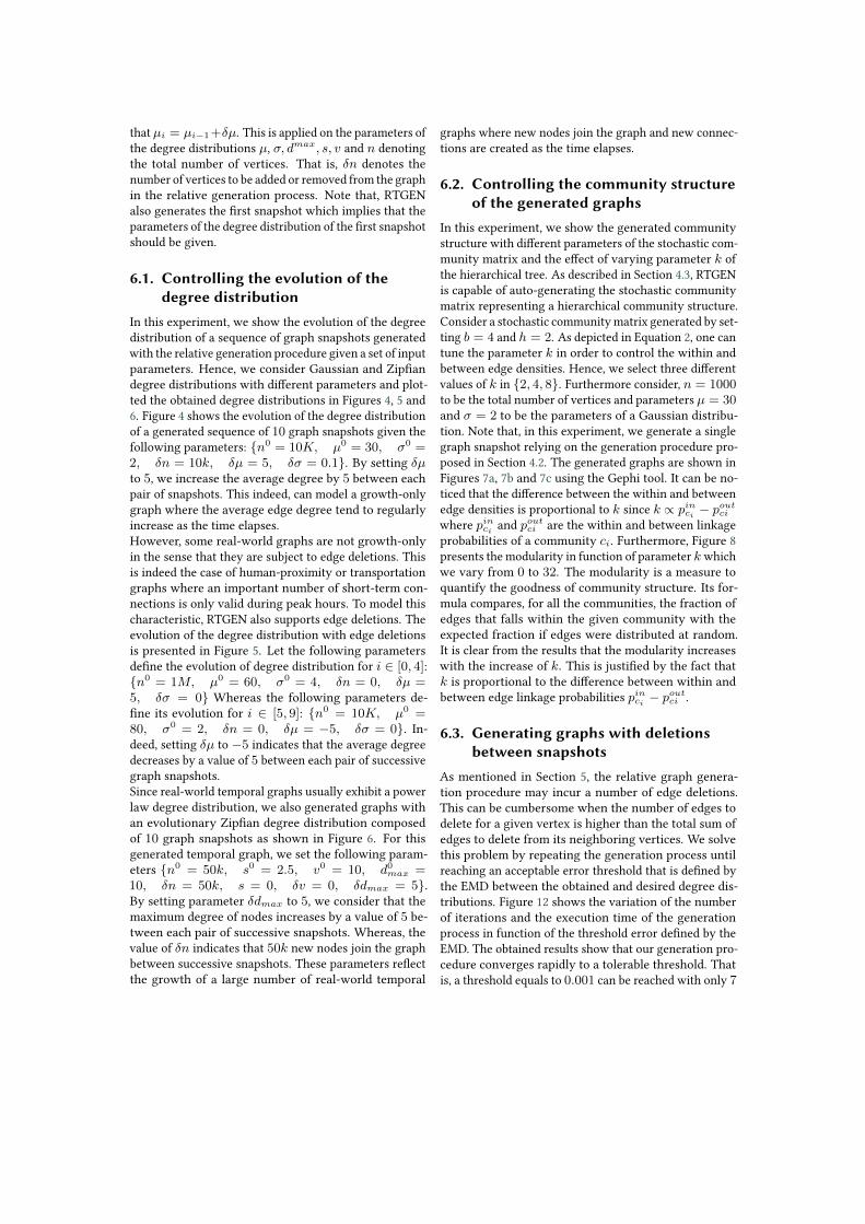
In this experiment, we show the generated communitystructure with different parameters of the stochastic com-munity matrix and the effect of varying parameter 𝑘 ofthe hierarchical tree. As described in Section 4.3, RTGENis capable of auto-generating the stochastic communitymatrix representing a hierarchical community structure.Consider a stochastic community matrix generated by set-ting 𝑏 = 4 and ℎ = 2. As depicted in Equation 2, one cantune the parameter 𝑘 in order to control the within andbetween edge densities. Hence, we select three differentvalues of 𝑘 in {2, 4, 8}. Furthermore consider, 𝑛 = 1000to be the total number of vertices and parameters 𝜇 = 30and 𝜎 = 2 to be the parameters of a Gaussian distribu-tion. Note that, in this experiment, we generate a singlegraph snapshot relying on the generation procedure pro-posed in Section 4.2. The generated graphs are shown inFigures 7a, 7b and 7c using the Gephi tool. It can be no-ticed that the difference between the within and betweenedge densities is proportional to 𝑘 since 𝑘 ∝ 𝑝𝑖𝑛𝑐𝑖 − 𝑝𝑜𝑢𝑡𝑐𝑖

where 𝑝𝑖𝑛𝑐𝑖 and 𝑝𝑜𝑢𝑡𝑐𝑖 are the within and between linkageprobabilities of a community 𝑐𝑖. Furthermore, Figure 8presents the modularity in function of parameter 𝑘 whichwe vary from 0 to 32. The modularity is a measure toquantify the goodness of community structure. Its for-mula compares, for all the communities, the fraction ofedges that falls within the given community with theexpected fraction if edges were distributed at random.It is clear from the results that the modularity increaseswith the increase of 𝑘. This is justified by the fact that𝑘 is proportional to the difference between within andbetween edge linkage probabilities 𝑝𝑖𝑛𝑐𝑖 − 𝑝𝑜𝑢𝑡𝑐𝑖 .

6.3. Generating graphs with deletionsbetween snapshots

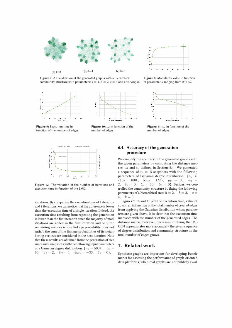
As mentioned in Section 5, the relative graph genera-tion procedure may incur a number of edge deletions.This can be cumbersome when the number of edges todelete for a given vertex is higher than the total sum ofedges to delete from its neighboring vertices. We solvethis problem by repeating the generation process untilreaching an acceptable error threshold that is defined bythe EMD between the obtained and desired degree dis-tributions. Figure 12 shows the variation of the numberof iterations and the execution time of the generationprocess in function of the threshold error defined by theEMD. The obtained results show that our generation pro-cedure converges rapidly to a tolerable threshold. Thatis, a threshold equals to 0.001 can be reached with only 7

(a) k=2 (b) k=4 (c) k=8

Figure 7: A visualization of the generated graphs with a hierarchicalcommunity structure with parameters: 𝑏 = 4, ℎ = 2, 𝑐 = 4 and a varying 𝑘.

Figure 8: Modularity value in functionof parameter 𝑘 ranging from 0 to 32.

Figure 9: Execution time infunction of the number of edges.

Figure 10: 𝜀𝑑 in function of thenumber of edges.

Figure 11: 𝜀𝑐 in function of thenumber of edges.

Figure 12: The variation of the number of iterations andexecution time in function of the EMD.

iterations. By comparing the execution time of 1 iterationand 7 iterations, we can notice that the difference is lowerthan the execution time of a single iteration. Indeed, theexecution time resulting from repeating the generationis lower than the first iteration since the majority of mod-ifications are added in the first iteration and only theremaining vertices whose linkage probability does notsatisfy the sum of the linkage probabilities of its neigh-boring vertices are considered in the next iteration. Notethat these results are obtained from the generation of twosuccessive snapshots with the following input parametersof a Gaussian degree distribution: {𝑛0 = 500𝑘, 𝜇0 =60, 𝜎0 = 2, 𝛿𝑛 = 0, 𝛿𝑚𝑢 = −30, 𝛿𝜎 = 0}.

6.4. Accuracy of the generationprocedure

We quantify the accuracy of the generated graphs withthe given parameters by computing the distance met-rics 𝜀𝑑 and 𝜀𝑐 defined in Section 5.4. We generateda sequence of 𝑛 = 5 snapshots with the followingparameters of Gaussian degree distribution: {𝑛0 ∈{10𝑘, 100𝑘, 500𝑘, 1𝑀}, 𝜇0 = 30, 𝜎0 =2, 𝛿𝑛 = 0, 𝛿𝜇 = 10, 𝛿𝜎 = 0}. Besides, we con-trolled the community structure by fixing the followingparameters of a hierarchical tree: ℎ = 2, 𝑏 = 2, 𝑐 =4, 𝑘 = 0.

Figures 9, 10 and 11 plot the execution time, value of𝜀𝑑 and 𝜀𝑐 in function of the total number of created edgesfrom applying the Gaussian distribution whose parame-ters are given above. It is clear that the execution timeincreases with the number of the generated edges. Thedistance metric, however, decreases implying that RT-GEN approximates more accurately the given sequenceof degree distribution and community structure as thetotal number of edges grows.

7. Related workSynthetic graphs are important for developing bench-marks for assessing the performance of graph-orienteddata platforms, when real graphs are not publicly avail-

able or expensive to obtain. This has been the incentiveto design models and generators, which are very use-ful for evaluating the efficiency of graph managementtechniques as storage, query evaluation, indexing, parti-tioning, etc.

An extensive work has been posited for the genera-tion of static graphs. For instance, a special emphasishas been placed to control the degree distribution of thegenerated graphs. In this context, many graph genera-tors were designed such as RTG [3], RMAT [4] and itsgeneralisation Kronecker [5] producing only Power-Lawdistributions. Since real-world graphs are not limitedto power-law distributions, BTER [6] and its extensionDarwini [7] and GMark [8] produce graphs with any userdefined distribution.

Another graph generation model producing a givendegree distribution is the CL model, forming the basisof the RTGEN tool. This model can be regarded as asuccessor of the Erdos-Rényi model [23] that is designedfor the generation of random graphs and a variant ofthe edge configuration model of Newman et al. [24].It was extensively discussed and reused [17, 28, 29, 30].We choose to extend this model for its simplicity andscalability.

Besides, a number of existing graph generators arecommunity-aware in the sense that they collect verticesthat are more densely connected between each otherthan they are with the rest of the graph, in separate oroverlapping subgraphs called communities [9, 10, 11].Although these generators preserve a given communitystructure, they fail to produce a graph with respect to agiven degree distribution. In this paper, we overcome thislimitation by allowing not only the generation of a givencommunity structure but also a given degree distribution.

Despite the extensive work posited on the genera-tion of non-temporal graphs, the generation of tempo-ral graphs has received much less attention. For in-stance, DANCer [31] is capable of generating temporal,community-aware property graphs. It separates opera-tions performed on communities (macro operations) fromoperations performed on vertices and edges (micro opera-tions). ComAwareNetGrowth [32] is a community-awaregraph generator that is capable of creating growth onlygraphs. APA (Attribute-Aware Preferential Attachment)[33] is a graph generator capable of creating growth-onlyproperty graphs based on a non-conventional triangleclosing. Instead of closing a triangle based on a uniformprobability given as an input parameter, their proposedmodel consists of closing a triangle based on the simi-larity between the candidate edge’s endpoints. WhileGMark [8] generates static graphs, EGG (Evolving GraphGenerator) [34] proposes an extension including evolv-ing properties attached to each vertex. EGG, however,disregard the topological changes to the network andnarrow the temporal evolution of the graph to property

updates. DSNG-M (dynamic social network generatorbased on modularity) [35] is a graph generator that iscapable of generating temporal graphs by flipping thedirection of edges of a given graph in order to satisfy arandomly chosen modularity value assigned to a singlegraph snapshot.

Some of the aforementioned graph generators producetemporal graphs with properties on nodes or vertices,which we do not address in this paper. None of them,however, allows the control of the evolution of the degreedistribution given ground truth parameters that describethis evolution. This challenge lead to the elaboration ofthe RTGEN tool that allows the approximation of anygiven sequence of degree distributions that describes theevolution of the graph. We firmly believe, that the degreedistribution is a key feature that characterizes graphs,hence, it should not be disregarded in graph generationtools.

8. ConclusionIn this paper, we addressed the generation of temporalgraphs that represents a critical challenge in the designof benchmarks specific for evaluating temporal graphmanagement systems. That is, we proposed RTGEN, atemporal graph generator that produces a sequence ofgraph snapshots whose community structure and evolu-tion of the degree distribution results from approximatinguser defined parameters. This generation procedure con-sists of relatively generating a graph snapshot from aprevious one by applying a number of atomic graph op-erations. Our generation technique relies on an Optimaltransport solver to approximate a user-defined sequenceof degree distributions while minimizing the number ofoperations needed to transform one snapshot into itssuccessor. We conducted a number of experiments thatvalidated the efficiency and accuracy of our generationprocedure. In the future, we are planning to include adynamic community structure to RTGEN. Indeed, thecommunities found in real-world graphs are subject tosplits, merges, shrinks or expansions which should alsobe modelled in synthetic graphs.

References[1] J. R. Clough, T. S. Evans, Time and citation net-

works, arXiv preprint arXiv:1507.01388 (2015).[2] M. D. Mueller, D. Hasenfratz, O. Saukh, M. Fierz,

C. Hueglin, Statistical modelling of particle numberconcentration in zurich at high spatio-temporal res-olution utilizing data from a mobile sensor network,Atmospheric Environment 126 (2016) 171–181.

[3] L. Akoglu, C. Faloutsos, Rtg: a recursive realisticgraph generator using random typing, in: Joint

European Conference on Machine Learning andKnowledge Discovery in Databases, Springer, 2009,pp. 13–28.

[4] D. Chakrabarti, Y. Zhan, C. Faloutsos, R-mat: Arecursive model for graph mining, in: Proceedingsof the 2004 SIAM International Conference on DataMining, SIAM, 2004, pp. 442–446.

[5] J. Leskovec, D. Chakrabarti, J. Kleinberg, C. Falout-sos, Z. Ghahramani, Kronecker graphs: An ap-proach to modeling networks, Journal of MachineLearning Research 11 (2010) 985–1042.

[6] T. G. Kolda, A. Pinar, T. Plantenga, C. Seshadhri, Ascalable generative graph model with communitystructure, SIAM Journal on Scientific Computing36 (2014) C424–C452.

[7] S. Edunov, D. Logothetis, C. Wang, A. Ching, M. Ka-biljo, Darwini: Generating realistic large-scale so-cial graphs, arXiv preprint arXiv:1610.00664 (2016).

[8] G. Bagan, A. Bonifati, R. Ciucanu, G. H. Fletcher,A. Lemay, N. Advokaat, gmark: Schema-drivengeneration of graphs and queries, IEEE Transac-tions on Knowledge and Data Engineering 29 (2016)856–869.

[9] P. W. Holland, K. B. Laskey, S. Leinhardt, Stochasticblockmodels: First steps, Social networks 5 (1983)109–137.

[10] B. Karrer, M. E. Newman, Stochastic blockmodelsand community structure in networks, Physicalreview E 83 (2011) 016107.

[11] B. Kamiński, P. Prałat, F. Théberge, Artificial bench-mark for community detection (abcd): Fast ran-dom graph model with community structure, arXivpreprint arXiv:2002.00843 (2020).

[12] P. Holme, Modern temporal network theory: acolloquium, The European Physical Journal B 88(2015) 234.

[13] E. Pitoura, Historical graphs: models, storage, pro-cessing, in: European Business Intelligence and BigData Summer School, Springer, 2017, pp. 84–111.

[14] Y. Miao, W. Han, K. Li, M. Wu, F. Yang, L. Zhou,V. Prabhakaran, E. Chen, W. Chen, Immortal-graph: A system for storage and analysis of tempo-ral graphs, ACM Transactions on Storage (TOS) 11(2015) 1–34.

[15] U. Khurana, A. Deshpande, Storing and analyz-ing historical graph data at scale, arXiv preprintarXiv:1509.08960 (2015).

[16] M. Haeusler, T. Trojer, J. Kessler, M. Farwick,E. Nowakowski, R. Breu, Chronograph: A ver-sioned tinkerpop graph database, in: InternationalConference on Data Management Technologies andApplications, Springer, 2017, pp. 237–260.

[17] F. Chung, L. Lu, The average distances in randomgraphs with given expected degrees, Proceedings ofthe National Academy of Sciences 99 (2002) 15879–

15882.[18] A. G. Labouseur, J. Birnbaum, P. W. Olsen, S. R.

Spillane, J. Vijayan, J.-H. Hwang, W.-S. Han, Theg* graph database: efficiently managing large dis-tributed dynamic graphs, Distributed and ParallelDatabases 33 (2015) 479–514.

[19] M. Then, T. Kersten, S. Günnemann, A. Kemper,T. Neumann, Automatic algorithm transformationfor efficient multi-snapshot analytics on temporalgraphs, Proceedings of the VLDB Endowment 10(2017) 877–888.

[20] C. Ren, E. Lo, B. Kao, X. Zhu, R. Cheng, On queryinghistorical evolving graph sequences, Proceedingsof the VLDB Endowment 4 (2011) 726–737.

[21] W. Aiello, F. Chung, L. Lu, A random graph modelfor power law graphs, Experimental Mathematics10 (2001) 53–66.

[22] F. Chung, L. Lu, Connected components in ran-dom graphs with given expected degree sequences,Annals of combinatorics 6 (2002) 125–145.

[23] P. Erdos, A. rényi on random graphs i, Publ. Math.Debrecen 6 (1959) 290–297.

[24] M. E. Newman, D. J. Watts, S. H. Strogatz, Randomgraph models of social networks, Proceedings of thenational academy of sciences 99 (2002) 2566–2572.

[25] R. Flamary, N. Courty, A. Gramfort, M. Z. Alaya,A. Boisbunon, S. Chambon, L. Chapel, A. Corenflos,K. Fatras, N. Fournier, L. Gautheron, N. T. Gayraud,H. Janati, A. Rakotomamonjy, I. Redko, A. Rolet,A. Schutz, V. Seguy, D. J. Sutherland, R. Tavenard,A. Tong, T. Vayer, Pot: Python optimal transport,Journal of Machine Learning Research 22 (2021)1–8. URL: http://jmlr.org/papers/v22/20-451.html.

[26] M. Bastian, S. Heymann, M. Jacomy, Gephi: an opensource software for exploring and manipulatingnetworks, in: Third international AAAI conferenceon weblogs and social media, 2009.

[27] V. D. Blondel, J.-L. Guillaume, R. Lambiotte, E. Lefeb-vre, Fast unfolding of communities in large net-works, Journal of statistical mechanics: theory andexperiment 2008 (2008) P10008.

[28] F. Chung, F. R. Chung, F. C. Graham, L. Lu, K. F.Chung, et al., Complex graphs and networks, 107,American Mathematical Soc., 2006.

[29] A. Pinar, C. Seshadhri, T. G. Kolda, The similaritybetween stochastic kronecker and chung-lu graphmodels, in: Proceedings of the 2012 SIAM Interna-tional Conference on Data Mining, SIAM, 2012, pp.1071–1082.

[30] M. Winlaw, H. DeSterck, G. Sanders, An in-depthanalysis of the chung-lu model, Technical Report,Lawrence Livermore National Lab.(LLNL), Liver-more, CA (United States), 2015.

[31] O. Benyahia, C. Largeron, B. Jeudy, O. R. Zaïane,Dancer: Dynamic attributed network with com-

munity structure generator, in: Joint EuropeanConference on Machine Learning and KnowledgeDiscovery in Databases, Springer, 2016, pp. 41–44.

[32] F. Gursoy, B. Badur, A community-aware networkgrowth model for synthetic social network genera-tion, arXiv preprint arXiv:1901.03629 (2019).

[33] A. Aghasadeghi, J. Stoyanovich, Generating evolv-ing property graphs with attribute-aware preferen-tial attachment, in: Proceedings of the Workshopon Testing Database Systems, 2018, pp. 1–6.

[34] K. Alami, R. Ciucanu, E. M. Nguifo, Synthetic graphgeneration from finely-tuned temporal constraints.,in: TD-LSG@ PKDD/ECML, 2017, pp. 44–47.

[35] B. Duan, W. Luo, H. Jiang, L. Ni, Dynamic socialnetworks generator based on modularity: Dsng-m, in: 2019 2nd International Conference on DataIntelligence and Security (ICDIS), IEEE, 2019, pp.167–173.