RPSRNet: End-to-End Trainable Rigid Point Set Registration ...

RPSRNet: End-to-End Trainable Rigid Point Set Registration Network using

Barnes-Hut 2D-Tree Representation

Sk Aziz Ali1,2 Kerem Kahraman1 Gerd Reis2 Didier Stricker1,2

1TU Kaiserslautern 2German Research Center for Artificial Intelligence (DFKI GmbH), Kaiserslautern

Abstract

We propose RPSRNet - a novel end-to-end trainable deep

neural network for rigid point set registration. For this

task, we use a novel 2D-tree representation for the input

point sets and a hierarchical deep feature embedding in

the neural network. An iterative transformation refinement

module of our network boosts the feature matching accu-

racy in the intermediate stages. We achieve an inference

speed of ∼12-15 ms to register a pair of input point clouds

as large as ∼250K. Extensive evaluations on (i) KITTI

LiDAR-odometry and (ii) ModelNet-40 datasets show that

our method outperforms prior state-of-the-art methods –

e.g., on the KITTI dataset, DCP-v2 by 1.3 and 1.5 times, and

PointNetLK by 1.8 and 1.9 times better rotational and trans-

lational accuracy respectively. Evaluation on ModelNet40

shows that RPSRNet is more robust than other benchmark

methods when the samples contain a significant amount of

noise and disturbance. RPSRNet accurately registers point

clouds with non-uniform sampling densities, e.g., LiDAR

data, which cannot be processed by many existing deep-

learning-based registration methods.

1. Introduction

Rigid point set registration (RPSR) is indispensable

in numerous computer vision and graphics applications –

e.g., camera pose estimation [2, 63], LiDAR-based odome-

try [74, 38], 3D reconstruction of partial scenes [30], simul-

taneous localization and mapping tasks [46], to name a few.

An RPSR method estimates the rigid motion field, parame-

terized by rotation (R ∈ SO(D)) and translation (t ∈ RD),

of a moving sensor from the given pair of D-dimensional

point clouds (source and target).

Generally, different types of input data from diverse ap-

plication areas pose distinct challenges to registration meth-

ods, e.g., (i) LiDAR data contains large number of points

with non-uniform sampling density, (ii) partial scans ob-

tained from structured-light sensors or multi-view camera

systems contain a large number of points with small amount

of overlap between the point clouds, (iii) RGB-D sensors,

Figure 1. Rigid Point Set Registration using Barnes-Hut (BH)

2D-tree Representation. The center-of-masses (CoMs) and

point-densities () of non-empty tree-nodes are computed for the

respective BH-trees of the source and target. These two attributes

are input to our RPSRNet which has global feature-embedding

blocks employing tree-convolution operations on the nodes. Fi-

nally, we regress rigid rotation (R ∈ SO(D)) and translation

(t ∈ RD) parameters from output features.

such as Kinect, yield dense depth data with large displace-

ment between consecutive frames.

Classical RPSR Methods. Iterative Closest Point (ICP)

[10] and its many variants [29, 56, 36, 60, 70, 28, 23] are

the most widely used methods that alternate the nearest cor-

respondence search and transformation estimation steps at

every iteration. A comparative study [50] shows that sev-

eral ICP variants target a specific challenge, and many of

them are prone to converge in bad local-minima. Coher-

ent Point Drift (CPD) [44] is another state-of-the-art ap-

proach from the class of probabilistic RPSR methods. Simi-

lar to CPD, GMMReg [11], FilterReg [21], and HGMR [19]

are also probabilistic RPSR methods that treat the data as

Gaussian mixture models. The probabilistic models for

rigid alignment gives more robustness against noisy input

than ICP [10]. Recently physics-based approaches, e.g.,

GA [25], BH-RGA [26], FGA [4], and [1, 3], are appearing

computationally faster and more robust than ICP or CPD.

These methods assume that the point clouds are astrophys-

ical particles with masses and obtain the optimal alignment

by defining a motion model for the source in a simulated

gravitational field. However, most of the above methods

13100

run on CPUs and do not scale to register large point clouds,

e.g., LiDAR scans. Due to this, often handcrafted [18] or

automatically extracted [58, 57] feature descriptors are iter-

atively sampled using RANSAC [53] to obtain true corre-

spondence matches. On the other hand, Fast Global Regis-

tration (FGR) [77] replaces the RANSAC step with a robust

global optimization technique to obtain true matches.

DNN-based Point Processing Registration Methods. A

recent survey [39] shows that many contributions are made

to the development of deep neural networks (DNNs) for

point cloud processing (PCP) tasks [51, 52, 69, 5, 66, 67,

42, 30, 32, 13, 62, 71, 48, 47, 40, 61, 41], e.g., classification

and segmentation [51, 52, 69], correspondence and geomet-

ric feature matching [24, 35], up-sampling [72], and down-

sampling [47]. Rigid point-set registration using DNNs ap-

peared recently [20, 5, 66, 67, 42, 30, 48, 71, 13]. El-

baz et al. [20] introduce the LORAX algorithm for large

scale point set registration using super-point representa-

tion. PointNetLK [5] is the first RPSR method which

uses PointNet [51] (w/o its T-net component) to obtain

the global feature-embedding of source and target. The

method further uses the iterative Lucas and Kanade (LK)

method to obtain the transformation optimizing the dis-

tance between global features. Unlike PointNetLK, the re-

cent RPSR method Deep Closet Point (DCP) [66] chooses

DGCNN [68] to obtain the feature embedding and a Trans-

former network [17] to learn contextual residuals between

them. PRNet [67] is an extension of DCP [66] to solve

a matching sharpness issue. Deep Global Registration

(DGR) [13], [16], and 3DRegNet [48] are among the lat-

est methods to report better accuracy than FGR [77] for

registering partial-to-partial scans. DGR takes fully con-

volutional geometric features (FCGF) [15] and trains a

high dimensional convolutional network [14] to classify in-

liers/outliers from the input FCGF descriptors. Finally, a

weighted Procrustes [27] using inlier weights estimate the

transformation. 3DRegNet [48] method also employs a

classifier, similar to the inlier/outlier classification block of

DGR, but using deep ResNet [31] layers, followed by dif-

ferentiable Procrustes [27] to align the scans. Notably, both

3DRegNet and DGR have ∼4 times and ∼10 higher runtime

than DCP [66]. Some other RPSR methods using DNNs are

AlignNet-3D [30], DeepGMR [73] and DeepVCP [42].

Problems in DNN-based Point Cloud Processing. Gen-

erally, DNNs on 3D point clouds give more intuitive high

dimensional geometric features learned from the given sam-

ples. Although, the convolution operations are not straight

forward for DNNs on point clouds because they can be

unordered, irregular and unstructured. Voxel-based [43]

or shallow grid-based [54] representations use volumet-

ric convolution which is very memory demanding (O(N3)where N is the voxel resolution) and can only be applied

to very small problems. In contrast, multilayer perceptron

(MLP) based convolution in [51, 52, 69, 72] operate on

sub-sampled versions of the point clouds. Thus, the local

correlation between the latent-features are inefficiently es-

tablished using random neighborhood search in MLP-based

methods. Another critical disadvantage of methods relying

on PointNet [51] (or its extension [52]) is that deconvolu-

tion is inapplicable. RPMNet [71], which is another Point-

Net [51] reliant RPSR method, shows that it requires points’

normals to be computed beforehand for robust alignment.

Additionally, the inference time, a crucial parameter for

real-time applications, of several recent DNN-based meth-

ods [71, 48, 13] are not on a par with DCP [66] or Deep-

VCP [42]. Among the DNN based approaches of RPSR, no

method is available so far which addresses the aforemen-

tioned issues.

2D-Tree Based Methods for Point Cloud Processing.

2D-tree (e.g., octree in 3D or quadtree in 2D) representa-

tion [76] of a point cloud is more memory efficient to en-

code local correlation among the points inside a tree-cell as

they can share the same input signals. Unlike regular grids,

2D-tree representation free up the empty cells, which are of-

ten more than 50% for sparse point clouds, from being com-

puted. Moreover, it provides hierarchical correlations be-

tween the neighborhood cells. FGA [4] and BH-RGA [26]

are the latest physics-based RPSR methods to use Barnes-

Hut (BH) 2D-tree representation of point clouds. FGA

shows state-of-the-art alignment accuracy and the fastest

speed among the classical methods. DNN-based methods

for shape reconstruction from a single image [62], point

cloud classification and segmentation (PCCS) [37, 65], real-

time 3D scene analysis [64], shape retrieval [55], and large

LiDAR data compression [32] have all appeared in last three

years which claim 2D-tree as more efficient learning rep-

resentation for point clouds. Although, there is no RPSR

method that addresses the aforementioned problems of pre-

vious learning-based approaches and simultaneously uti-

lizes the efficacy of 2D-tree representation.

In this paper, we present the first DNN-based RPSR

method using a novel Barnes-Hut (BH) [8] 2D-tree repre-

sentation of input point clouds (see Fig. 1). At first, we build

a BH-tree by recursively subdividing the normalized bound-

ing space of an input point cloud up to a limiting depth d

(Sec. 2). A tree with maximum depth d = 6 or 7 (i.e., equiv-

alent to 643 or 1283 voxels in 3D) gives a fine level of gran-

ularity for our proposed DNN to process. Except from the

root node, which contains all the points, the internal nodes

of the 2D-tree encapsulate varying number of points. Hence,

the center-of-masses (CoMs) and the inverse densities (IDs)

of the nodes, computed at each depth, are the representative

attributes of a BH-tree. Besides, the neighbors of a given

node are easily retrievable using established indexing and

hash maps [7] for 2D-tree. With this input representation,

Sec. 3 describes the complete pipeline of RPSRNet. To this

13101

end, we design a single DNN block – hierarchical feature

extraction (HFE) – with d hidden layers for global feature

extraction. Two sub-blocks under HFE – namely hierar-

chical position feature embedding (HPFE) and hierarchical

density feature embedding (HDFE) respectively – learn the

positional and density features, respectively. We apply late-

fusion between HPFE and HDFE that results in a density

adaptive embedding. As a result, learned-features become

homogeneous for the input point clouds with non-uniform

point sampling densities (e.g., LiDAR scans). The final

block of our RPSRNet, inspired by DCP-v2 [66], contains a

relational network [59]i with an integrated transformer [6],

and a differentiable singular value decomposition (SVD)ii

module. We further refine the estimation with an iterative

rigid alignment architecture with multiple alignment-passes

for a single pair of input sample (See Fig. 3 and Sec. 3.3).

Contributions. The overall contributions and promising

characteristics of this work are as follows:

• A novel BH 2D-tree representation of input point sets.

• An end-to-end trainable rigid registration network with

real time inference on dense point clouds using the fol-

lowing components:

1. HPFE and HDFE using 2D-tree convolution

2. Rigid transformation estimation using relational

network and differentiable SVD.

3. A multi-pass architecture for iterative transfor-

mation (R, t) refinement (similar to [67])

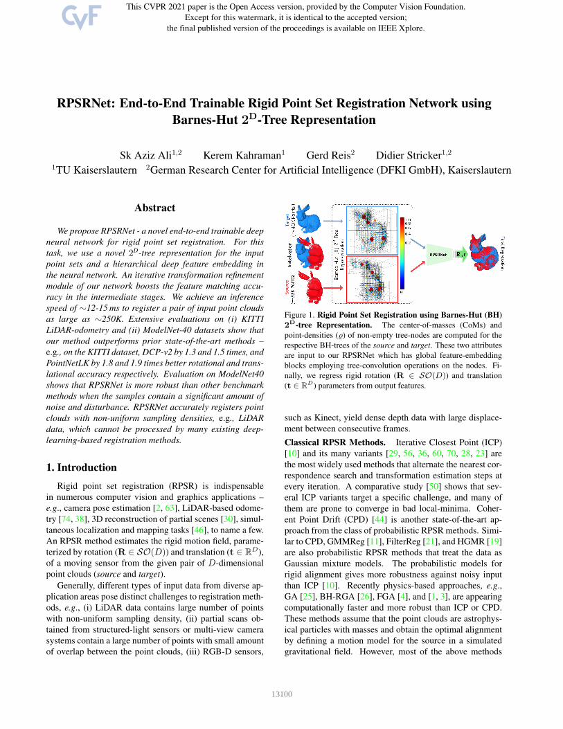
2. The Proposed BH 2D-Tree Construction

Figure 2. Barnes-Hut 2D-Tree construction and nodes.

Given a pair of misaligned input point clouds, a source

Y ∈ RM×(D+c) and a target X ∈ R

N×(D+c), we build

Barnes-Hut (BH) [8] 2D-trees τY and τX on them. The

ito extract the correspondence weights from our hierarchical deep fea-

ture embedding of source and targetiito estimate rotation and translation parameters.

trees (τY and τX) are defined by their respective sets of

nodes (NY

d and NX

d ) and the parent-child relationships

among them at different depths d = 1, 2, . . .. Every point in

Y and X is a D-dimensional position vector, often associ-

ated with an additional c-dimensional input feature channel.

The input features can be RGB color channels, local point

densities, or other attributes. Although BH-tree is gener-

alizable for D-dimensional input data, we describe further

details and notations w.r.t 3D data (i.e. D = 3) for easier

understanding. The following steps describe how to build

a BH octree (i.e. 23 = 8 child octants per parent node) by

recursively subdividing the Euclidean space of an input:

1. We determine the extreme point positions, i.e., min,

max values along x, y, and z-axes, and split the whole

space (as root node) from its center into 23 cubical sub-

cells as its child nodes. The half-length of the cube is

called cell length r. Depending on the structure of the

input point clouds, if not a regular grid structure, the

child nodes can be empty, non-empty with more than

one point, and non-empty with exactly one point. We

call them null, internal, and leaf nodes (see Fig. 2-A).

2. For each internal node, we compute the center-of-mass

(CoM) µ ∈ R3 and inverse density (ID)iii − ∈ R

+

of the encapsulated points inside. These two attributes

(CoM and ID) of a leaf node are equivalent to the point

position and its local density.

3. We continue the subdivision of the internal nodes only

up to a maximum depth d0 if leaf node is not reached.

Fig.2-(B) illustrates the BH-tree CoMs of the nodes at dif-

ferent depths d = 2, 3, 4 and 5 with their color-coded (mag-

nitude order: red > green > blue) point densities . Further-

more, we establish the indexing of the nodes (Nd) as well as

their neighborhood indices (κd) at every depth d using a la-

bel array (Ld) as hash key to retrieve the parent-child infor-

mation. For instance, the child nodes at depth d of Nd−1,i

(a non-empty parent node i at depth d− 1) will be indexed

in order of the Morton’s ’Z’ curve: {23 ·i+1, . . . , 23 ·i+8}.

The supplement has exemplary indexing.

3. The Proposed RPSRNet Method

In this section, we formulate the rigid alignment problem

between two BH-trees constructed on the input point cloud

pair, and then describe our RPSRNet model for this rigid

alignment task by highlighting its different components.

3.1. Mathematical Formulation

Rigid registration of a movable 3D point cloud Y ={y1, . . . ,yM} ∈ R

M×3 (i.e., source) with another point

iiiinspired by Monte-Carlo Importance Sampling Density – if m random

samples drawn from a meta-distribution function q(x) of a distribution

p(x), then expectation of sample can be expressed as a fraction of weights

w(x) =p(x)q(x)

, such that the normalized importance is∑m

i=1 w(xi) = 1.

13102

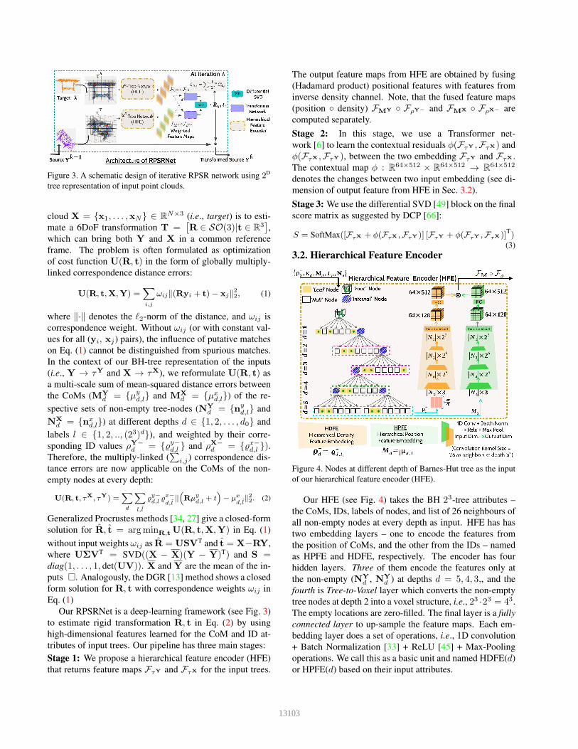
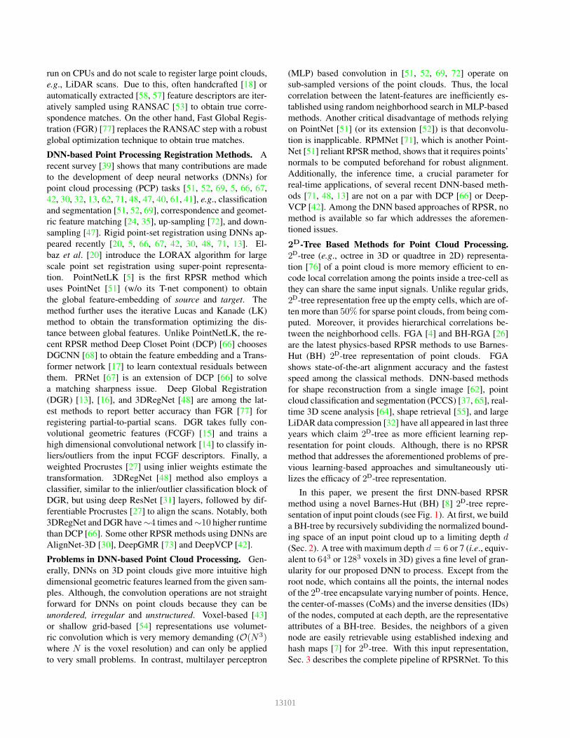
Figure 3. A schematic design of iterative RPSR network using 2D

tree representation of input point clouds.

cloud X = {x1, . . . ,xN} ∈ RN×3 (i.e., target) is to esti-

mate a 6DoF transformation T =[

R ∈ SO(3)|t ∈ R3]

,

which can bring both Y and X in a common reference

frame. The problem is often formulated as optimization

of cost function U(R, t) in the form of globally multiply-

linked correspondence distance errors:

U(R, t,X,Y) =∑

i,j

ωij‖(Ryi + t)− xj‖22, (1)

where ‖·‖ denotes the ℓ2-norm of the distance, and ωij is

correspondence weight. Without ωij (or with constant val-

ues for all (yi, xj) pairs), the influence of putative matches

on Eq. (1) cannot be distinguished from spurious matches.

In the context of our BH-tree representation of the inputs

(i.e., Y → τY and X → τX), we reformulate U(R, t) as

a multi-scale sum of mean-squared distance errors between

the CoMs (MY

d = {µyd,l} and MX

d = {µxd,l}) of the re-

spective sets of non-empty tree-nodes (NY

d = {nyd,l} and

NX

d = {nxd,l}) at different depths d ∈ {1, 2, . . . , d0} and

labels l ∈ {1, 2, .., (23)d}), and weighted by their corre-

sponding ID values ρY−

d = {y−d,l } and ρX−

d = {x−d,l }).Therefore, the multiply-linked (

∑

i,j) correspondence dis-

tance errors are now applicable on the CoMs of the non-

empty nodes at every depth:

U(R, t, τX, τY) =∑

d

∑

l,l

y−d,l

x−

d,l‖(

Rµyd,l

+ t

)

− µx

d,l‖22. (2)

Generalized Procrustes methods [34, 27] give a closed-form

solution for R, t = argminR,t U(R, t,X,Y) in Eq. (1)

without input weights ωij as R = USVT and t = X−RY,

where UΣVT = SVD((X − X)(Y − Y)T) and S =diag(1, . . . , 1, det(UV)). X and Y are the mean of the in-

puts �. Analogously, the DGR [13] method shows a closed

form solution for R, t with correspondence weights ωij in

Eq. (1)

Our RPSRNet is a deep-learning framework (see Fig. 3)

to estimate rigid transformation R, t in Eq. (2) by using

high-dimensional features learned for the CoM and ID at-

tributes of input trees. Our pipeline has three main stages:

Stage 1: We propose a hierarchical feature encoder (HFE)

that returns feature maps FτY and FτX for the input trees.

The output feature maps from HFE are obtained by fusing

(Hadamard product) positional features with features from

inverse density channel. Note, that the fused feature maps

(position ◦ density) FMY ◦ FρY− and FMX ◦ FρX− are

computed separately.

Stage 2: In this stage, we use a Transformer net-

work [6] to learn the contextual residuals φ(FτY ,FτX) and

φ(FτX ,FτY ), between the two embedding FτY and FτX .

The contextual map φ : R64×512 × R64×512 → R

64×512

denotes the changes between two input embedding (see di-

mension of output feature from HFE in Sec. 3.2).

Stage 3: We use the differential SVD [49] block on the final

score matrix as suggested by DCP [66]:

S = SoftMax([FτX + φ(FτX ,FτY )] [FτY + φ(FτY ,FτX)]T)(3)

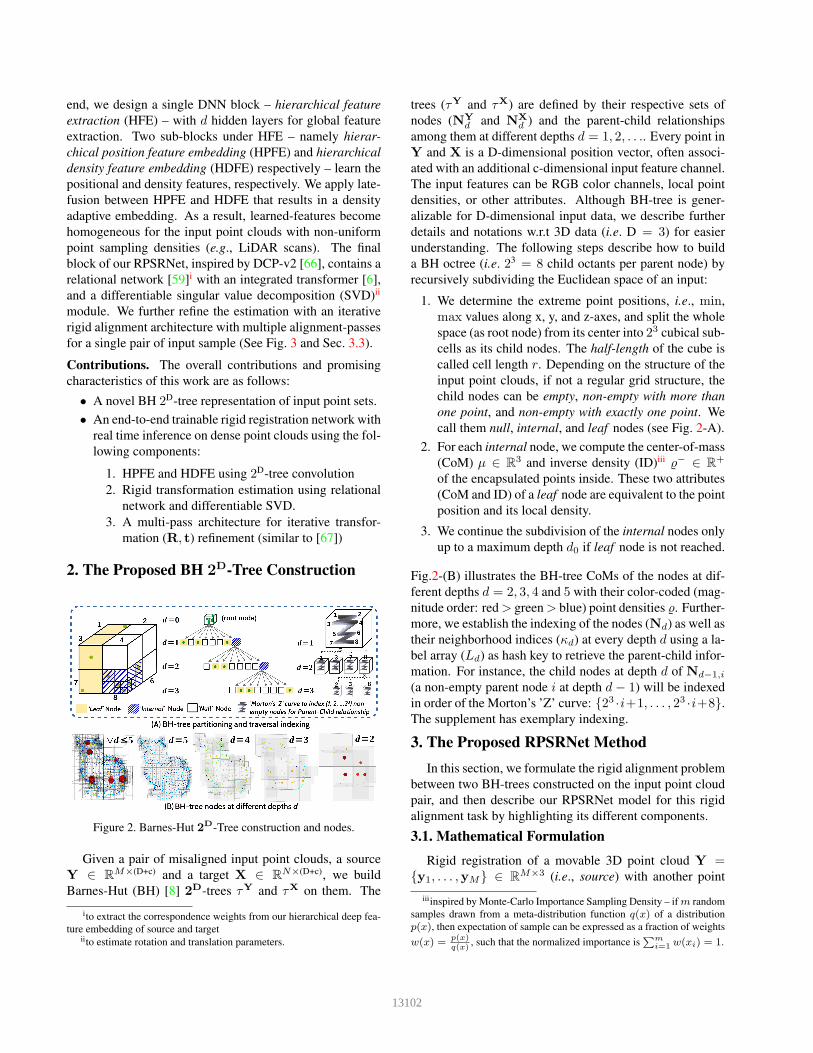
3.2. Hierarchical Feature Encoder

Figure 4. Nodes at different depth of Barnes-Hut tree as the input

of our hierarchical feature encoder (HFE).

Our HFE (see Fig. 4) takes the BH 23-tree attributes –

the CoMs, IDs, labels of nodes, and list of 26 neighbours of

all non-empty nodes at every depth as input. HFE has has

two embedding layers – one to encode the features from

the position of CoMs, and the other from the IDs – named

as HPFE and HDFE, respectively. The encoder has four

hidden layers. Three of them encode the features only at

the non-empty (NY

d , NY

d ) at depths d = 5, 4, 3,, and the

fourth is Tree-to-Voxel layer which converts the non-empty

tree nodes at depth 2 into a voxel structure, i.e., 23 ·23 = 43.

The empty locations are zero-filled. The final layer is a fully

connected layer to up-sample the feature maps. Each em-

bedding layer does a set of operations, i.e., 1D convolution

+ Batch Normalization [33] + ReLU [45] + Max-Pooling

operations. We call this as a basic unit and named HDFE(d)

or HPFE(d) based on their input attributes.

13103

Barnes-Hut 23-Tree Convolution / Pooling. To perform

the tree convolution operation, we use smart indexing of

tree nodes, parent-child relation order, and adjacency sys-

tem of their neighborhoods. Fig. 2-(A) shows a ‘Z’-curve

(known as Morton’s curve) traverse through nodes at the

current depth d and increase their label index l by 1 leaving

the empty node label as -1. If the parent node was empty,

the ‘Z’curve skips that octant. Hence, we keep an array for

the labels Ld at every depth to serve as hash map (See sup-

plementary material ). Next, for the convolution operation

on every non-empty node, 26 adjacent nodes from the same

depth are fetched. Notably adjacent sibling nodes can be

empty. At run time, we dispatch a zero filling operation on

those empty neighbors for indexed based (Ld) 1D convolu-

tion. In the reverse case, while Max-Pooling, information

flows from child to parent nodes. Hence the same operation

of zero filling is done on the empty siblings of a non-empty

parent (See supplement for for detailed example indexing

on a tree and operations like zero-filling and child-filling).

The following is the input and output feature dimensions at

depth d using weight filter W after 1D convolution:

Fout = Conv1D(W ∈ R|Nd|×26+1

,Fin ∈ R|Nd|×2(10−d)

) (4)

3.3. Iterative Registration Loss

RPSRNet predicts the final transformation in multiple

steps. On every internal iteration k, a combined loss LkR,t

on rotation: LkR

= ‖(Rkpred)

TRgt − I‖2, and translation:

Lkt= ‖(tkpred) − tgt‖

2 is minimized. Our combined loss

LkR,t and total loss LR,t using learnable scale parameters

σR and σt (for balanced learning of the components) are:

LkR,t = exp(−σR)Lk

R+ σR + exp(−σt)L

kt+ σt (5)

andLR,t =∑

k

(1

2)kLk

R,t, where k0 = max iteration.

The scale parameters σR and σt help the network to learn

the wide range of transformations.

4. Data Preparation and Evaluation Method

We evaluate on synthetic ModelNet40 [75] dataset which

contains 9843 training and 2468 test samples of CAD mod-

els under 40 different categories, and also KITTI LiDAR-

Odometry [22, 9] as several driving sequences.

ModelNet40 Dataset. In one setup (M1), we use all the

∼9.8K training and ∼2.4K testing samples under all 40 dif-

ferent object categories. In another setup (M2), to evalu-

ate the generalizability of our network, we choose a train-

ing set TM with shapes belonging to the first twenty cat-

egories, and testing set T ∗

M where shapes are from the

other twenty categories that are not seen during training.

All input samples are scaled between [−1, 1]. The tar-

get point clouds are obtained after transforming its clone

by random orientations (θx, θy, θz) ∈ (0◦, 45◦] and a ran-

dom linear translation (tx, ty, tz) ∈ [−0.5, 0.5]. To help

the deep networks better cope with the data disturbances,

another 950 training and 240 testing samples are ran-

domly selected to be preprocessed by four different set-

tings of noise or data disturbances on source point clouds

– (i) adding Gaussian ∼N (0, 0.02) and (ii) uniformly dis-

tributed noise ∼U(−1.0, 1.0) which are 20% of the to-

tal points in a sample, (iii) cropping a chunk (approx.

20%) of data, and (iv) jitter each point’s position with

a displacement tolerance 0.03. The choice of applying

one of the four options is random. We prepare five in-

stances of the validation sets with increasing level of noise

(1%, 5%, 10%, 20%, and 40%), jitter (increasing displace-

ment threshold), and crops (1%, 10%, 20%, 30%, and 40%).

KITTI Dataset. There are 22 driving sequences in

KITTI LiDAR odometry dataset. We prepare two se-

tups – in the first setup (K1-w/o), the ground points

are removed from each sample using the label informa-

tion from SemanticKITTI [9], and in the second setup

(K2-w) samples remain unchanged. The samples from

each driving sequence 00 to 07 are split into 70%, 20%,

and 10% as training, testing and validation sets and then

merged. The number of frames in the sequences are

4541, 1101, 4661, 801, 271, 2761, 1101, and 1101 respec-

tively. Source point clouds from any of these sets are ran-

domly selected frame-indices, whereas the corresponding

targets are with next fifth frame-indices. Our RPSRNet can

process point clouds with actual size. Due to the memory

and scalability issues, PointNetLK [5], DCP-v2 [66], and

CPD [44] use inputs down-sampled to 2048 points.

Evaluation Baselines. We compare state-of-the-art neural

network-based methods – DCP-v2 [66] and PointNetLK [5]

against our RPSRNet. We also evaluate several unsu-

pervised methods – ICP [10], FilterReg [21], CPD [44],

FGR [77], GAi [25, 26] – for broader analysis (see Sec. A

of the supplement for details on training and parameter set-

tings) and ignore some recent CNN-based methods [48, 71,

13] that have higher run time (> 150 milliseconds).

Evaluation Metrics. We use angular deviation ϕ between

the ground truth and predicted rotation matrices (Rgt,R),

and similarly, the Euclidean distance error ∆t between the

ground truth and predicted translations (tgt, t) as:

ϕ = cos−1(

0.5(tr(

RTgtR

)

− 1))

, ∆t = ‖tgt − t‖. (6)

5. Experiments and Results

5.1. Indoor Scenes: Synthetic ModelNet40

Since the DCP and PointNetLK provide the pre-trained

model only on the clean version of the ModelNet40 [75]

dataset, we retrain the networks on our augmented versions

iA GPU implementation

13104

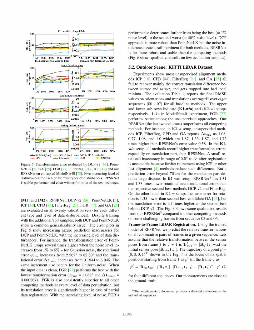
Figure 5. Transformation error evaluated by DCP-v2 [66], Point-

NetLK [5], GA [25], FGR [77], FilterReg [21] , ICP [10] and our

RPSRNet on corrupted ModelNet40 [75]. Five increasing level of

disturbances for each of the four types of disturbances. RPSRNet

is stable performer and clear winner for most of the test instances.

(M1) and (M2). RPSRNet, DCP-v2 [66], PointNetLK [5],

ICP [10], CPD [44], FilterReg [21], FGR [77], and GA [25]

are evaluated on all twenty validation sets (for each differ-

ent type and level of data disturbances). Despite training

with the additional 950 samples, both DCP and PointNetLK

show a common generalizability issue. The error plots in

Fig. 5 show increasing nature prediction inaccuracies for

DCP and PointNetLK, with the increasing level of data dis-

turbances. For instance, the transformation error of Point-

NetLK jumps several times higher when the noise level in-

creases from 1% to 5% – for Gaussian noise, the rotational

error ϕrmse increases from 2.267◦ to 82.69◦ and the trans-

lational error ∆trmse increases from 0.1844 to 5.945. The

same increment also occurs for the Uniform noise. When

the input data is clean, FGR [77] performs the best with the

lowest transformation error (ϕrmse = 1.082◦ and ∆trmse =

0.000267). FGR is also consistently superior to all other

competing methods at every level of data perturbation, but

its translation error is significantly higher in case of partial

data registration. With the increasing level of noise, FGR’s

performance deteriorates further from being the best (at 1%noise level) to the second-worst (at 40% noise level). DCP

approach is more robust than PointNetLK but the noise in-

tolerance issue is still pertinent for both methods. RPSRNet

is far more robust and stable than the competing methods

(Fig. 6 shows qualitative results on few evaluation samples).

5.2. Outdoor Scene: KITTI LiDAR Dataset

Experiments show most unsupervised alignment meth-

ods ICP [10], CPD [44], FilterReg [21], and GA [25] all

fail to recover mainly the correct translation difference be-

tween source and target, and gets trapped into bad local

minima. The evaluation Table 1, reports the final RMSE

values on orientations and translations averagediv over eight

sequences (00 - 07) for all baseline methods. The upper

and lower sub-rows indicate (K1-w/o) and (K2-w) setups

respectively. Like in ModelNet40 experiment, FGR [77]

performs better among the unsupervised approaches. Our

RPSRNet (the last two columns) outperforms all competing

methods. For instance, in K2-w setup, unsupervided meth-

ods ICP, FilterReg, CPD and GA reports ∆trmse as 1.08,

0.77, 1.08, and 1.0 which are 1.87, 1.33, 1.87, and 1.72

times higher than RPSRNet’s error value 0.58. In the K1-

w/o setup, all methods record higher transformation errors,

especially on translation part, than RPSRNet. A small ro-

tational inaccuracy in range of 0.5◦ to 3◦ after registration

is acceptable because further refinement using ICP or other

fast alignment [4] methods reduce such difference. But a

prediction error beyond 70 cm for the translation part de-

notes large dispute. In K1-w/o setup: RPSRNet3 has 1.31

and 1.33 times lower rotational and translational errors than

the respective second best methods DCP-v2 and FilterReg.

On the other hand, in K2-w setup: the same error for rota-

tion is 1.35 lower than second best candidate GA [25], but

the translation error is 1.1 times higher as the second best

behind DCP-v2. The Fig. 8 shows some qualitative results

from our RPSRNet3 compared to other competing methods

on some challenging frames from sequence 03 and 06.

Frame-to-Frame LiDAR Registration. Using the trained

model of RPSRNet, we predict the relative transformations

on all consecutive pairs of frames in a given sequence. Lets

assume that the relative transformation between the sensor

poses from frame f to f + 1 is Tf4×4 = [Rf tf ] w.r.t the

initial sensor pose [Rinit, tinit]. The trajectory of a point ~p =(0, 0, 0, 1)T shown in the Fig. 7 is the locus of its spatial

positions starting from frame 1 as ~p1 till the frame f as

~pf = [Rinittinit] · ([Rf tf ] · [Rf−1 tf−1] · · · [R1 t1])

−1 · ~p. (7)

for four different sequences. Our measurements are close to

the ground-truth.

ivThe supplementary document provides a detailed evaluation on the

individual sequences

13105

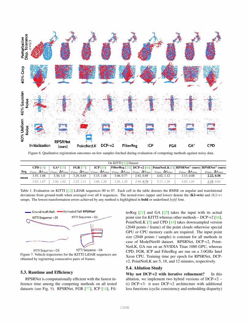
Figure 6. Qualitative registration outcomes on few samples fetched during evaluation of competing methods against noisy data.

On KITTI [22] Dataset

Seq.

CPD [44]

ϕrmse, ∆trmse

GA* [25]

ϕrmse, ∆trmse

FGR [77]

ϕrmse, ∆trmse

ICP [10]

ϕrmse, ∆trmse

FilterReg [21]

ϕrmse, ∆trmse

DCP-v2 [66]

ϕrmse, ∆trmse

PointNetLK [5]

ϕrmse, ∆trmse

RPSRNet1 (ours)

ϕrmse, ∆trmse

RPSRNet3 (ours)

ϕrmse, ∆trmse

mean3.55, 1.08 3.30, 1.0 3.29, 0.85 3.15, 1.08 3.08, 0.77 2.92, 0.89 4.02, 1.12 3.13, 0.88 2.22, 0.58

3.03, 1.07 2.94, 1.02 3.25, 1.11 3.06, 1.20 3.26, 1.20 2.96, 0.76 5.17, 1.20 3.03, 1.01 2.18, 0.84

Table 1. Evaluation on KITTI [22] LiDAR sequences 00 to 07. Each cell in the table denotes the RMSE on angular and translational

deviations from ground-truth when averaged over all 8 sequences. The nested-rows (upper and lower) denote the (K1-w/o) and (K2-w)

setups. The lowest transformation errors achieved by any method is highlighted in bold or underlined bold font.

Figure 7. Vehicle trajectories for the KITTI LiDAR sequences are

obtained by registering consecutive pairs of frames.

5.3. Runtime and Efficiency

RPSRNet is computationally efficient with the fastest in-

ference time among the competing methods on all tested

datasets (see Fig. 9). RPSRNet, FGR [77], ICP [10], Fil-

terReg [21] and GA [25] takes the input with its actual

point size for KITTI whereas other methods – DCP-v2 [66],

PointNetLK [5] and CPD [44] takes downsampled version

(2048 points / frame) of the point clouds otherwise special

GPU or CPU memory cards are required. The input point

size (2048 points / sample) is constant for all methods in

case of ModelNet40 dataset. RPSRNet, DCP-v2, Point-

NetLK, GA run on an NVIDIA Titan 1080 GPU, whereas

CPD, FGR, ICP and FilterReg are run on a 3.0GHz Intel

Xeon CPU. Training time per epoch for RPSRNet, DCP-

v2, PointNetLK are 5, 18, and 12 minutes, respectively.

5.4. Ablation Study

Why not DCP-v2 with iterative refinement? In this

ablation, we implement two hybrid versions of DCP-v2 –

(i) DCP-v3: it uses DCP-v2 architecture with additional

loss functions (cyclic consistency and embedding disparity)

13106

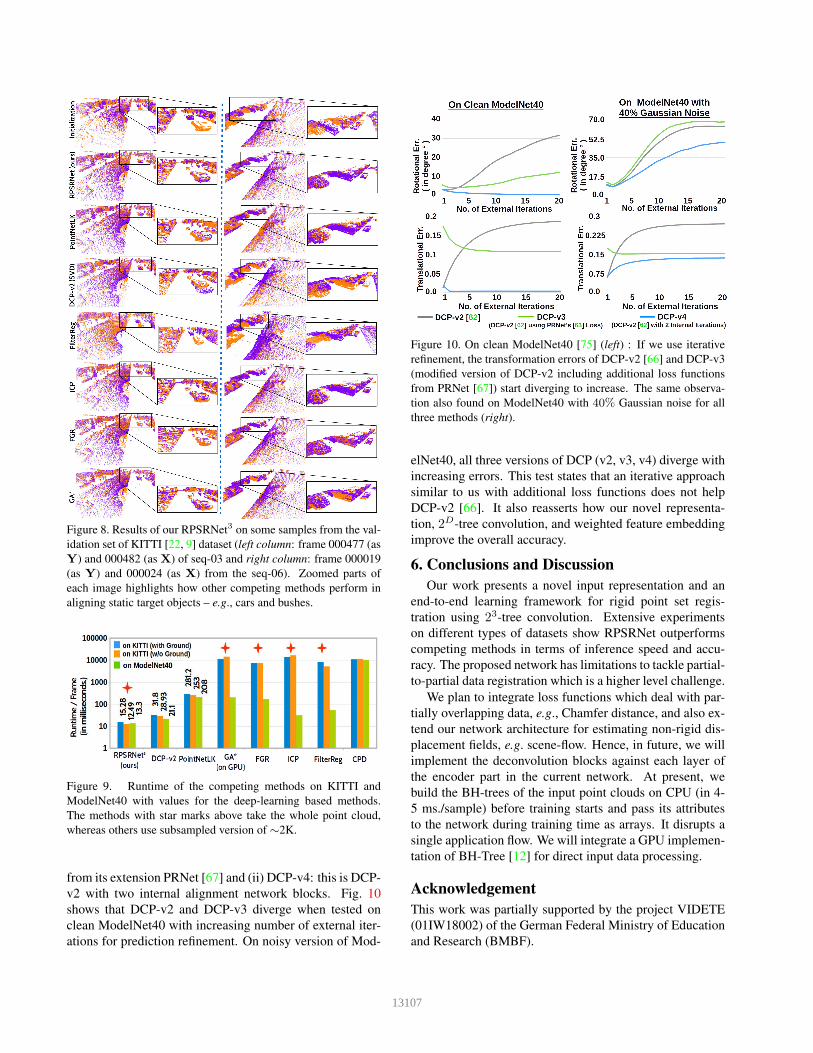
Figure 8. Results of our RPSRNet3 on some samples from the val-

idation set of KITTI [22, 9] dataset (left column: frame 000477 (as

Y) and 000482 (as X) of seq-03 and right column: frame 000019

(as Y) and 000024 (as X) from the seq-06). Zoomed parts of

each image highlights how other competing methods perform in

aligning static target objects – e.g., cars and bushes.

Figure 9. Runtime of the competing methods on KITTI and

ModelNet40 with values for the deep-learning based methods.

The methods with star marks above take the whole point cloud,

whereas others use subsampled version of ∼2K.

from its extension PRNet [67] and (ii) DCP-v4: this is DCP-

v2 with two internal alignment network blocks. Fig. 10

shows that DCP-v2 and DCP-v3 diverge when tested on

clean ModelNet40 with increasing number of external iter-

ations for prediction refinement. On noisy version of Mod-

Figure 10. On clean ModelNet40 [75] (left) : If we use iterative

refinement, the transformation errors of DCP-v2 [66] and DCP-v3

(modified version of DCP-v2 including additional loss functions

from PRNet [67]) start diverging to increase. The same observa-

tion also found on ModelNet40 with 40% Gaussian noise for all

three methods (right).

elNet40, all three versions of DCP (v2, v3, v4) diverge with

increasing errors. This test states that an iterative approach

similar to us with additional loss functions does not help

DCP-v2 [66]. It also reasserts how our novel representa-

tion, 2D-tree convolution, and weighted feature embedding

improve the overall accuracy.

6. Conclusions and Discussion

Our work presents a novel input representation and an

end-to-end learning framework for rigid point set regis-

tration using 23-tree convolution. Extensive experiments

on different types of datasets show RPSRNet outperforms

competing methods in terms of inference speed and accu-

racy. The proposed network has limitations to tackle partial-

to-partial data registration which is a higher level challenge.

We plan to integrate loss functions which deal with par-

tially overlapping data, e.g., Chamfer distance, and also ex-

tend our network architecture for estimating non-rigid dis-

placement fields, e.g. scene-flow. Hence, in future, we will

implement the deconvolution blocks against each layer of

the encoder part in the current network. At present, we

build the BH-trees of the input point clouds on CPU (in 4-

5 ms./sample) before training starts and pass its attributes

to the network during training time as arrays. It disrupts a

single application flow. We will integrate a GPU implemen-

tation of BH-Tree [12] for direct input data processing.

Acknowledgement

This work was partially supported by the project VIDETE

(01IW18002) of the German Federal Ministry of Education

and Research (BMBF).

13107

References

[1] Swapna Agarwal and Brojeshwar Bhowmick. 3d point cloud

registration with shape constraint. International Conference

on Image Processing (ICIP), pages 2199–2203, 2017. 1

[2] Aitor Aldoma, Markus Vincze, Nico Blodow, David Gossow,

Suat Gedikli, Radu Bogdan Rusu, and Gary Bradski. Cad-

model recognition and 6dof pose estimation using 3d cues. In

International Conference on Computer Vision (ICCV) Work-

shops, 2011. 1

[3] Sk Aziz Ali, Vladislav Golyanik, and Didier Stricker.

NRGA: Gravitational Approach for Non-rigid Point Set Reg-

istration. In International Conference on 3D Vision (3DV),

2018. 1

[4] Sk Aziz Ali, Kerem Kahraman, Christian Theobalt, Didier

Stricker, and Vladislav Golyanik. Fast Gravitational Ap-

proach for Rigid Point Set Registration with Ordinary Dif-

ferential Equations. arXiv e-prints, 2020. 1, 2, 6

[5] Yasuhiro Aoki, Hunter Goforth, Rangaprasad Arun Srivat-

san, and Simon Lucey. Pointnetlk: Robust and efficient point

cloud registration using pointnet. In CVPR, 2019. 2, 5, 6, 7

[6] Noam Shazeer Ashish Vaswani, Niki Parmar, Jakob Uszkor-

eit, Llion Jones, Aidan N Gomez, Lukasz Kaiser, , and Illia

Polo-sukhin. Attention is all you need. In Advances in Neu-

ral Information Processing (NIPS), 2017. 3, 4

[7] Michael Bader. Space-filling curves: an introduction with

applications in scientific computing, volume 9. Springer Sci-

ence & Business Media, 2012. 2

[8] J. Barnes and P. Hut. A hierarchical o(n log n) force-

calculation algorithm. Nature, 324:446–449, 1986. 2, 3

[9] J. Behley, M. Garbade, A. Milioto, J. Quenzel, S. Behnke,

C. Stachniss, and J. Gall. SemanticKITTI: A Dataset for

Semantic Scene Understanding of LiDAR Sequences. In In-

ternational Conf. on Computer Vision (ICCV), 2019. 5, 8

[10] P. J. Besl and N. D. McKay. A method for registration of

3-d shapes. Transactions on Pattern Analysis and Machine

Intelligence (TPAMI), 14(2):239–256, 1992. 1, 5, 6, 7

[11] Bing Jian and B. C. Vemuri. A robust algorithm for point

set registration using mixture of gaussians. In International

Conference on Computer Vision (ICCV), 2005. 1

[12] Martin Burtscher and Keshav Pingali. Chapter 6 - an efficient

cuda implementation of the tree-based barnes hut n-body al-

gorithm. In GPU Computing Gems Emerald Edition, Appli-

cations of GPU Computing Series, pages 75 – 92. Boston,

2011. 8

[13] Christopher Choy, Wei Dong, and Vladlen Koltun. Deep

global registration. In Computer Vision and Pattern Recog-

nition (CVPR), 2020. 2, 4, 5

[14] Christopher Choy, Junha Lee, Rene Ranftl, Jaesik Park, and

Vladlen Koltun. High-dimensional convolutional networks

for geometric pattern recognition. In Computer Vision and

Pattern Recognition (CVPR), 2020. 2

[15] Christopher Choy, Jaesik Park, and Vladlen Koltun. Fully

convolutional geometric features. In International Confer-

ence on Computer Vision, pages 8958–8966, 2019. 2

[16] H. Deng, T. Birdal, and S. Ilic. 3d local features for direct

pairwise registration. In Computer Vision and Pattern Recog-

nition (CVPR), 2019. 2

[17] Jacob Devlin, Ming-Wei Chang, Kenton Lee, and Kristina

Toutanova. Bert: Pre-training of deep bidirectional

transformers for language understanding. arXiv preprint

arXiv:1810.04805, 2018. 2

[18] Zhen Dong, Bisheng Yang, Yuan Liu, Fuxun Liang, Bijun

Li, and Yufu Zang. A novel binary shape context for 3d local

surface description. 130:431 – 452, 2017. 2

[19] Benjamin Eckart, Kihwan Kim, and Jan Kautz. Hgmr: Hi-

erarchical gaussian mixtures for adaptive 3d registration. In

European Conference on Computer Vision (ECCV), 2018. 1

[20] Gil Elbaz, Tamar Avraham, and Anath Fischer. 3d point

cloud registration for localization using a deep neural net-

work auto-encoder. Computer Vision and Pattern Recogni-

tion (CVPR), pages 2472–2481, 2017. 2

[21] Wei Gao and Russ Tedrake. Filterreg: Robust and effi-

cient probabilistic point-set registration using gaussian filter

and twist parameterization. In Computer Vision and Pattern

Recognition (CVPR), 2019. 1, 5, 6, 7

[22] Andreas Geiger, Philip Lenz, Christoph Stiller, and Raquel

Urtasun. Vision meets robotics: The kitti dataset. Interna-

tional Journal of Robotics Research (IJRR), 2013. 5, 7, 8

[23] N. Gelfand, L. Ikemoto, S. Rusinkiewicz, and M. Levoy. Ge-

ometrically stable sampling for the icp algorithm. In Inter-

national Conference on 3-D Digital Imaging and Modeling,

2003. 3DIM 2003. Proceedings., pages 260–267, 2003. 1

[24] Zan Gojcic, Caifa Zhou, Jan D Wegner, and Andreas Wieser.

The perfect match: 3d point cloud matching with smoothed

densities. In Computer Vision and Pattern Recognition

(CVPR), pages 5545–5554, 2019. 2

[25] Vladislav Golyanik, Sk Aziz Ali, and Didier Stricker. Gravi-

tational approach for point set registration. Computer Vision

and Pattern Recognition (CVPR), 2016. 1, 5, 6, 7

[26] Vladislav Golyanik, Christian Theobalt, and Didier Stricker.

Accelerated gravitational point set alignment with altered

physical laws. In International Conference on Computer Vi-

sion (ICCV), 2019. 1, 2, 5

[27] John C Gower. Generalized procrustes analysis. Psychome-

trika, 40(1):33–51, 1975. 2, 4

[28] Sebastien Granger and Xavier Pennec. Multi-scale em-icp:

A fast and robust approach for surface registration. In Eu-

ropean Conference on Computer Vision (ECCV). Springer

Berlin Heidelberg, 2002. 1

[29] MA Greenspan and M. Yurick. Approximate k-d tree search

for efficient icp. In International Conference on Recent Ad-

vances in 3D Digital Imaging and Modeling (3DIM), 2003.

1

[30] Johannes Groß, Aljosa Osep, and Bastian Leibe. Alignnet-

3d: Fast point cloud registration of partially observed ob-

jects. In International Conference on 3D Vision (3DV), pages

623–632. IEEE, 2019. 1, 2

[31] K. He, X. Zhang, S. Ren, and J. Sun. Deep residual learn-

ing for image recognition. In Computer Vision and Pattern

Recognition (CVPR), 2016. 2

[32] Lila Huang, Shenlong Wang, Kelvin Wong, Jerry Liu, and

Raquel Urtasun. Octsqueeze: Octree-structured entropy

model for lidar compression. In Computer Vision and Pat-

tern Recognition (CVPR), 2020. 2

13108

[33] Sergey Ioffe and Christian Szegedy. Batch normalization:

Accelerating deep network training by reducing internal co-

variate shift. In International Conference on Machine Learn-

ing (ICML), 2015. 4

[34] Wolfgang Kabsch. A solution for the best rotation to re-

late two sets of vectors. Acta Crystallographica Section A:

Crystal Physics, Diffraction, Theoretical and General Crys-

tallography, 32(5):922–923, 1976. 4

[35] Marc Khoury, Qian-Yi Zhou, and Vladlen Koltun. Learning

compact geometric features. In International Conference on

Computer Vision (ICCV), pages 153–161, 2017. 2

[36] Michael Korn, Martin Holzkothen, and Josef Pauli. Color

supported generalized-icp. Computer Vision Theory and Ap-

plications (VISAPP), 3:592–599, 2014. 1

[37] Huan Lei, Naveed Akhtar, and Ajmal Mian. Octree guided

cnn with spherical kernels for 3d point clouds. Computer

Vision and Pattern Recognition (CVPR), 2019. 2

[38] Qing Li, Shaoyang Chen, Cheng Wang, Xin Li, Chenglu

Wen, Ming Cheng, and Jonathan Li. Lo-net: Deep real-time

lidar odometry. In Computer Vision and Pattern Recognition

(CVPR), 2019. 1

[39] Weiping Liu, Jia Sun, Wanyi Li, Ting Hu, and Peng Wang.

Deep learning on point clouds and its application: A survey.

Sensors, 19(19), 2019. 2

[40] Yongcheng Liu, Bin Fan, Gaofeng Meng, Jiwen Lu, Shim-

ing Xiang, and Chunhong Pan. Densepoint: Learning

densely contextual representation for efficient point cloud

processing. In International Conference on Computer Vision

(ICCV), 2019. 2

[41] Yongcheng Liu, Bin Fan, Shiming Xiang, and Chunhong

Pan. Relation-shape convolutional neural network for point

cloud analysis. In Computer Vision and Pattern Recognition

(CVPR), 2019. 2

[42] Weixin Lu, Guowei Wan, Yao Zhou, Xiangyu Fu, Pengfei

Yuan, and Shiyu Song. Deepvcp: An end-to-end deep neural

network for point cloud registration. In Computer Vision and

Pattern Recognition (CVPR), pages 12–21, 2019. 2

[43] Daniel Maturana and Sebastian Scherer. Voxnet: A 3d con-

volutional neural network for real-time object recognition.

In 2015 IEEE/RSJ International Conference on Intelligent

Robots and Systems (IROS), pages 922–928. IEEE. 2

[44] A. Myronenko and X. Song. Point set registration: Coherent

point drift. Transactions on Pattern Analysis and Machine

Intelligence (TPAMI), 32(12):2262–2275, 2010. 1, 5, 6, 7

[45] Vinod Nair and Geoffrey E. Hinton. Rectified linear units im-

prove restricted boltzmann machines. In International Con-

ference on Machine Learning (ICML), 2010. 4

[46] R. A. Newcombe, S. Izadi, O. Hilliges, D. Molyneaux, D.

Kim, A. J. Davison, P. Kohi, J. Shotton, S. Hodges, and A.

Fitzgibbon. Kinectfusion: Real-time dense surface mapping

and tracking. In International Symposium on Mixed and Aug-

mented Reality (ISMAR), 2011. 1

[47] Ehsan Nezhadarya, Ehsan Taghavi, Ryan Razani, Bingbing

Liu, and Jun Luo. Adaptive hierarchical down-sampling for

point cloud classification. In Conference on Computer Vision

and Pattern Recognition (CVPR), June. 2

[48] G. Dias Pais, Pedro Miraldo, Srikumar Ramalingam, Jac-

into C. Nascimento, Venu Madhav Govindu, and Rama Chel-

lappa. 3dregnet: A deep neural network for 3d point regis-

tration. 2019. 2, 5

[49] Adam Paszke, Sam Gross, Soumith Chintala, Gregory

Chanan, Edward Yang, Zachary DeVito, Zeming Lin, Al-

ban Desmaison, Luca Antiga, , and Adam Lerer. Automatic

differentiation in pytorch. 2017. 4

[50] Francis Pomerleau, Francoisand Colas and Stephane Sieg-

wart, Rolandand Magnenat. Comparing icp variants on real-

world data sets. Autonomous Robots, 34(3):133–148, 2013.

1

[51] Charles R Qi, Hao Su, Kaichun Mo, and Leonidas J Guibas.

Pointnet: Deep learning on point sets for 3d classification

and segmentation. In Computer Vision and Pattern Recogni-

tion (CVPR), pages 652–660, 2017. 2

[52] Charles Ruizhongtai Qi, Li Yi, Hao Su, and Leonidas J

Guibas. Pointnet++: Deep hierarchical feature learning on

point sets in a metric space. In Advances in neural informa-

tion processing systems, pages 5099–5108, 2017. 2

[53] Rahul Raguram, Jan-Michael Frahm, and Marc Pollefeys. A

comparative analysis of ransac techniques leading to adap-

tive real-time random sample consensus. In European Con-

ference on Computer Vision (ECCV), 2008. 2

[54] Gernot Riegler, Ali Osman Ulusoy, and Andreas Geiger.

Octnet: Learning deep 3d representations at high resolutions.

In Computer Vision and Pattern Recognition (CVPR), pages

3577–3586, 2017. 2

[55] Gernot Riegler, Osman Ulusoy, and Andreas Geiger. Oct-

net: Learning deep 3d representations at high resolutions. In

Computer Vision and Pattern Recognition (CVPR), 2017. 2

[56] Szymon Rusinkiewicz and Marc Levoy. Efficient variants

of the ICP algorithm. In International Conference on 3D

Digital Imaging and Modeling (3DIM), 2001. 1

[57] R. B. Rusu, N. Blodow, and M. Beetz. Fast point feature

histograms (fpfh) for 3d registration. In International Con-

ference on Robotics and Automation (ICRA), 2009. 2

[58] R. B. Rusu, N. Blodow, Z. C. Marton, and M. Beetz. Align-

ing point cloud views using persistent feature histograms. In

International Conference on Intelligent Robots and Systems

(IROS), 2008. 2

[59] Adam Santoro, David Raposo, David G Barrett, Mateusz

Malinowski, Razvan Pascanu, Peter Battaglia, and Timothy

Lillicrap. A simple neural network module for relational rea-

soning. In Advances in neural information processing sys-

tems, pages 4967–4976, 2017. 3

[60] Aleksandr Segal, Dirk Hahnel, and Sebastian Thrun.

Generalized-icp. In Robotics: Science and Systems V, Uni-

versity of Washington, Seattle, USA, June 28 - July 1, 2009,

2009. 1

[61] Hang Su, Varun Jampani, Deqing Sun, Subhransu Maji,

Evangelos Kalogerakis, Ming-Hsuan Yang, and Jan Kautz.

SPLATNet: Sparse lattice networks for point cloud process-

ing. In Computer Vision and Pattern Recognition (CVPR),

2018. 2

[62] Maxim Tatarchenko, Alexey Dosovitskiy, and Thomas Brox.

Octree generating networks: Efficient convolutional archi-

13109

tectures for high-resolution 3d outputs. In International Con-

ference on Computer Vision, 2017. 2

[63] S. Umeyama. Least-squares estimation of transformation pa-

rameters between two point patterns. Transactions on Pat-

tern Analysis and Machine Intelligence (TPAMI), 13(4):376–

380, 1991. 1

[64] F. Wang, Y. Zhuang, H. Gu, and H. Hu. Octreenet: A novel

sparse 3-d convolutional neural network for real-time 3-d

outdoor scene analysis. IEEE Transactions on Automation

Science and Engineering, 17(2):735–747, 2020. 2

[65] Peng-Shuai Wang, Yang Liu, Yu-Xiao Guo, Chun-Yu Sun,

and Xin Tong. O-CNN: Octree-based Convolutional Neu-

ral Networks for 3D Shape Analysis. ACM Transactions on

Graphics (SIGGRAPH), 36(4), 2017. 2

[66] Yue Wang and Justin Solomon. Deep closest point: Learning

representations for point cloud registration. In International

Conference on Computer Vision (ICCV), pages 3523–3532,

2019. 2, 3, 4, 5, 6, 7, 8

[67] Yue Wang and Justin Solomon. Prnet: Self-supervised learn-

ing for partial-to-partial registration. In Advances in Neural

Information Processing Systems (NIPS), pages 8812–8824,

2019. 2, 3, 8

[68] Yue Wang, Yongbin Sun, Ziwei Liu, Sanjay E Sarma,

Michael M Bronstein, and Justin M Solomon. Dynamic

graph cnn for learning on point clouds. ACM Transactions

on Graphics (TOG), 38(5):1–12, 2019. 2

[69] Wenxuan Wu, Zhongang Qi, and Li Fuxin. Pointconv: Deep

convolutional networks on 3d point clouds. In Computer Vi-

sion and Pattern Recognition, pages 9621–9630, 2019. 2

[70] J. Yang, H. Li, and Y. Jia. Go-icp: Solving 3d registration ef-

ficiently and globally optimally. In International Conference

on Computer Vision (ICCV), 2013. 1

[71] Z. J. Yew and G. H. Lee. Rpm-net: Robust point matching

using learned features. In 2020 IEEE/CVF Conference on

Computer Vision and Pattern Recognition (CVPR), 2020. 2,

5

[72] Wang Yifan, Shihao Wu, Hui Huang, Daniel Cohen-Or, and

Olga Sorkine-Hornung. Patch-based progressive 3d point set

upsampling. In Computer Vision and Pattern Recognition

(CVPR), pages 5958–5967, 2019. 2

[73] Wentao Yuan, Benjamin Eckart, Kihwan Kim, Varun Jam-

pani, Dieter Fox, and Jan Kautz. Deepgmr: Learning latent

gaussian mixture models for registration. In European Con-

ference on Computer Vision (ECCV). Springer, 2020. 2

[74] Ji Zhang and Sanjiv Singh. Low-drift and real-time lidar

odometry and mapping. Autonomous Robots, 41(2):401416,

2016. 1

[75] Zhirong Wu, S. Song, A. Khosla, Fisher Yu, Linguang

Zhang, Xiaoou Tang, and J. Xiao. 3d shapenets: A deep rep-

resentation for volumetric shapes. In Computer Vision and

Pattern Recognition (CVPR), 2015. 5, 6, 8

[76] Kun Zhou, Minmin Gong, Xin Huang, and Baining Guo.

Data-parallel octrees for surface reconstruction. Transac-

tions on visualization and computer graphics, 17(5):669–

681, 2010. 2

[77] Qian-Yi Zhou, Jaesik Park, and Vladlen Koltun. Fast global

registration. In European Conference on Computer Vision

(ECCV), 2016. 2, 5, 6, 7

13110