Rotifer species richness along an altitudinal gradient in the Alps: Rotifer species richness in the Alps

Page 1

RESEARCHPAPER

Rotifer species richness along analtitudinal gradient in the Alpsgeb_556 895..904

Ulrike Obertegger1*, Bertha Thaler2 and Giovanna Flaim1

1IASMA Research and Innovation Centre,

FEM, Environment and Natural Resources

Area, I-38010 San Michele all’Adige (TN),

Italy, 2Provincial Environmental Protection

Agency, Bozen, I-39055 Leifers (BZ), Italy

ABSTRACT

Aim Biodiversity patterns along altitudinal gradients are less studied in aquaticthan terrestrial systems, even though aquatic sites provide a more homogeneousenvironment independent of moisture constraints. We studied the altitudinalspecies richness pattern for planktonic rotifers in freshwater lakes and identified theenvironmental predictors for which altitude is a proxy.

Location Two hundred and eighteen lakes of Trentino–South Tyrol (Italy) in theeastern Alps; lakes covered 98% (range 65–2960 m above sea level) of the altitudinalgradient in the Alps.

Methods We performed: (1) linear regression between species richness and alti-tude to evaluate the general pattern, (2) multiple linear regression between speciesrichness and environmental predictors excluding altitude to identify the mostimportant predictors, and (3) linear regression between the residuals of the bestmodel of step (2) and altitude to investigate any additional explanatory power ofaltitude. Selection of environmental predictors was based on limnological impor-tance and non-parametric Spearman correlations. We applied ordinary leastsquares regression, generalized linear, and generalized least squares modelling toselect the most statistically appropriate model.

Results Rotifer species richness showed a monotonic decrease with altitude inde-pendent of scale effects. Species richness could be explained (R2 = 51%) by lake areaas a proxy for habitat diversity, reactive silica and total phosphorus as proxies forproductivity, water temperature as a proxy for energy, nitrate as a proxy for humaninfluence and north–south and east–west directions as covariates. These predictorscompletely accounted for the species richness–altitude pattern, and altitude had noadditional effect on species richness.

Main conclusions The linear decrease of species richness along the altitudinalgradient was related to the interplay of habitat diversity, productivity, heat contentand human influence. These factors are the same in terrestrial and aquatic habitats,but the greater environmental stability of aquatic systems seems to favour a linearpattern.

KeywordsAlps, biodiversity, habitat diversity, Italy, lakes, productivity, regressionanalysis, rotifers, temperature, zooplankton.

*Correspondence: Ulrike Obertegger, IASMA,Research and Innovation Centre, FEM,Environment and Natural Resources Area, ViaEdmund Mach, 1, I-38010 San Micheleall’Adige (TN), Italy.E-mail: [email protected]

INTRODUCTION

Understanding the factors that govern species richness is a fun-

damental issue for ecologists regardless of the habitat studied,

especially as ecosystem functioning is related to biodiversity.

Studies that address this topic are particularly important given

current concerns about loss of biodiversity with global climate

change (Nyman et al., 2005). To comprehend the mechanisms

that determine biodiversity patterns, species richness along

spatial gradients such as latitude and altitude are increasingly

being studied (e.g. Nyman et al., 2005; Hessen et al., 2007). In

particular, focus has been put on altitudinal gradients because

Global Ecology and Biogeography, (Global Ecol. Biogeogr.) (2010) 19, 895–904

© 2010 Blackwell Publishing Ltd DOI: 10.1111/j.1466-8238.2010.00556.xwww.blackwellpublishing.com/geb 895

Page 2

they offer more constant ecological conditions and history with

respect to other spatial gradients while at the same time are

linked to several environmental variables giving beneficial

insights for both theoretical and applied research on biodiversity

(Rowe, 2009). The species richness–altitude relationship gener-

ally shows two main patterns (i.e. decreasing or unimodal)

depending on the main attributes of scale (i.e. the unit of sam-

pling and the geographical space covered) (Rahbek, 2005). Spe-

cifically, the exclusion of altitudes lower than 500 m or higher

than 2000 m above sea level (a.s.l.) leads to a biased species

richness–altitude relationship (Rahbek, 2005; Nogués-Bravo

et al., 2008). Furthermore, the different extent of human impact

at different altitudes is decisive for observing different altitudi-

nal patterns of species richness in nature (Nogués-Bravo et al.,

2008).

Besides the need for a comprehensive altitudinal gradient,

terrestrial studies on altitudinal processes are often con-

founded by covariance between altitude and regional peculiari-

ties, moisture constraints (Körner, 2007) and temperature

fluctuations (Reynolds, 1998). On the contrary, the more

homogeneous character of aquatic ecosystems (e.g. marine,

Smith & Brown, 2002; freshwater, Hessen et al., 2007) offers

the possibility to investigate altitudinal gradients independent

of such terrestrial peculiarities. In contrast to the connectivity

of terrestrial and marine habitats, however, inland waters have

well-defined boundaries, are isolated and are surrounded by an

unsuitable landscape leading to a patchy environment (Rey-

nolds, 1998; Jankowski & Weyhenmeyer, 2006; Scheffer & van

Geest, 2006). Lakes are also unique because of their internal

physical gradients such as light, temperature and oxygen that

structure plankton communities. Aquatic organisms, because

of characteristics such as short life cycles, reduced size struc-

tures and efficient resource uptake, generally show faster

responses to environmental changes than terrestrial organisms,

corroborating the viewpoint that freshwater studies can con-

tribute much to the general understanding of ecosystem pro-

cesses (Reynolds, 1998).

However, most studies on altitudinal gradients focus on ter-

restrial species (Rahbek, 1995, 2005; Currie & Kerr, 2008;

Nogués-Bravo et al. 2008 and references therein), and four

main groups of hypothesis have been identified to explain

species richness–altitude patterns. The climatic hypothesis

considers temperature and humidity (e.g. Kluge et al., 2006;

McCain, 2007) and energy and ecosystem productivity (e.g.

Davies et al., 2007), the spatial hypothesis considers area (e.g.

Williams, 1964; MacArthur & Wilson, 1967), randomness and

neutral theories (e.g. Hubbell, 2001) and spatial constraints

(e.g. Colwell & Lees, 2000), the historical hypothesis considers

historical and evolutionary processes (e.g. Wiens & Donoghue,

2004) and the biotic hypothesis considers source–sink dynam-

ics (e.g. Grytnes et al., 2006) as the main drivers for the

observed patterns.

Less is known about altitudinal gradients in aquatic ecosys-

tems (Bêche & Statzner, 2009 and references therein); the species

richness–altitude relationship has been studied for only a few

aquatic taxa: phytoplankton (local species richness, Jankowski &

Weyhenmeyer, 2006), aquatic plants (Jones et al., 2003), crusta-

ceans (Hessen et al., 2007), stream macroinvertebrates (local

species richness, Jacobsen, 2004) and molluscs (Sturm, 2007)

show a linear decrease, while stream macroinvertebrates (altitu-

dinal bands, Jacobsen, 2004), chironomids (Nyman et al., 2005),

phytoplankton (altitudinal bands, Jankowski & Weyhenmeyer,

2006) and fish (Li et al., 2009) show a hump-shaped pattern

with altitude. Some of these nonlinear patterns can be attributed

to rescue effects that maintain the presence of species in unsuit-

able habitats by continuous colonization from suitable habitats

(Jacobsen, 2004) and investigating species richness in an

ecotonal transitional zone (Nyman et al., 2005) probably subject

to source–sink effects that result in species flow from optimal to

suboptimal sites. Both of these similar effects can inflate the

assessment of species richness (Jones et al., 2003; Grytnes &

McCain, 2007). In aquatic habitats, hypotheses on the species

richness–altitude pattern rely on area and climatic variables

(Jones et al., 2003; Li et al., 2009), geometric constraints, dis-

persal, environmental heterogeneity, productivity (Jankowski &

Weyhenmeyer, 2006; Hessen et al., 2007; Li et al., 2009) and

temperature (Nyman et al., 2005; Hessen et al., 2007).

In this paper, we focus on the mechanisms shaping species

richness in lakes over a complete altitudinal gradient in the

Alps. The Alps in particular are an especially interesting study

site because they provide broad ecological gradients, can serve

as a template for the many mountainous regions world-wide

and are a hotspot of biodiversity in Europe. We focused on

planktonic monogonont rotifers as a general model to study

biodiversity because they are: (1) widely distributed, (2) an

important component of the pelagic food web, and (3) readily

susceptible to changes in their environment (Reynolds, 1998;

Lampert & Sommer, 2007). In addition, a comprehensive study

on rotifer richness in relation to altitude is lacking, and only

ancillary information is available: monogonont rotifer richness

in high-altitude lakes decreases with altitude (Jersabek, 1995)

and Synchaeta species show a preference for lakes of specific

altitudinal belts (Obertegger et al., 2008). Our aims were

twofold: (1) investigate the pattern of the rotifer richness–

altitude relationship (linear or hump-shaped) and ascertain its

consistency across altitudinal bands, and (2) identify the envi-

ronmental predictors for which altitude is a proxy. We selected

variables related to habitat diversity, productivity, energy and

human influence covering the different factors outlined in ter-

restrial as well as freshwater studies to develop a holistic model

of the species richness–altitude relationship in lakes. While the

outcome of the first issue is of a more theoretical nature

necessary for the development of a unifying theory on

biodiversity, the outcome of the latter issue is relevant for

a mechanistic understanding of the environment and species

richness patterns sensu Gotelli et al. (2009). Our dataset, with

a wide range of predictors representing important environ-

mental gradients, offers a unique opportunity to study these

interconnected research questions. In addition, we provide a

better understanding of the processes behind the richness–

altitude relationship, an issue that is still controversial (Rowe,

2009).

U. Obertegger et al.

Global Ecology and Biogeography, 19, 895–904, © 2010 Blackwell Publishing Ltd896

Page 3

MATERIALS AND METHODS

Study sites and data acquisition

We studied rotifer species richness in relation to altitude in 218

lakes in the Trentino–South Tyrol region in the eastern Alps

(Italy), sampled during the summers of 1996–2008 (Fig. 1).

These lakes ranged from 65 to 2960 m a.s.l. with an average of

four lakes every 100 m, and covered 98.3% of the Alpine altitu-

dinal gradient (value according to Körner, 2007). The lakes

sampled spanned a wide range of environmental variables

(Table 1) and reflected the altitudinal distribution of lakes in the

study area (Fig. 2). The range of the north–south and east–west

direction was limited to less than 2°; therefore these spatial

parameters were not considered as gradients, but were impor-

tant for accounting for spatial autocorrelation (see statistical

modelling below). Species lists and environmental data were

either based on published data (45 lakes: IASMA, 1996–2000;

Salmaso & Naselli-Flores, 1999; Cantonati et al., 2002; Cantonati

& Lazzara, 2006) or provided directly by the authors. Zooplank-

ton samples were generally taken from the deepest part of the

lake with a plankton net (50 mm) and were preserved in 4%

formalin or 20% alcohol. The coordinates of the lakes’ centroids

were available on three different coordinate systems: the Univer-

sal Transverse Mercator (UTM) 32N/WGS84 (South Tyrol), the

Gauss Boaga/Rome40 W (Trentino), and the lat/long/WGS84

(Trentino); all the geographic positions were harmonized in the

lat/long/WGS84 system applying a datum-shift correction using

seven parameters specific to the study area.

Data treatment and statistical modelling

Species richness on a continuous altitudinal scale was calculated

as the number of rotifer taxa found in each lake. Species richness

at different altitudinal resolutions was calculated as the mean

Figure 1 Location of the 218 lakes sampled in Trentino–SouthTyrol (Italy). Continuous lines represent major rivers, filled circlesrepresent sampling sites.

Figure 2 Altitudinal distribution of lakes in Trentino–SouthTyrol for 100 m intervals. Black bars are mapped lakes (n = 667)and white bars are sampled lakes (n = 218).

Table 1 Minimum (min), maximum(max), median and mean values for themajor predictors of lakes sampled (n =218).

Parameter Min Max Median Mean

Altitude (m) 65 2960 2245 1954

Area (ha) < 1 36,800 2 185

Depth (m) 1 350 6 12

TP (mg l-1) 1 220 9 15

N-NO3 (mg l-1) 6 2165 174 232

N:P < 1 1017 40 68

Si (mg l-1) 0.1 10.7 1.3 1.7

SO4 (mg l-1) 0.2 94.9 3.6 8.7

Conductivity (mS cm-1) 4 504 45 98

Temperature (°C) 2.0 26.7 12.0 12.6

Latitude (N) 45°39′59″ 46°56′47″ 46°32′12″ 46°30′11″Longitude (E) 10°23′12″ 12°20′43″ 11°13′20″ 11°16′54″

Area is lake surface area, temperature is surface water temperature, TP is total phosphorus, and Si isreactive silica.

Rotifer species richness in the Alps

Global Ecology and Biogeography, 19, 895–904, © 2010 Blackwell Publishing Ltd 897

Page 4

value of species richness for lakes within bands of different

altitudinal widths (100 m, 200 m, 300 m and 400 m band

widths) over the 3000-m range. In terrestrial studies, standard-

ization of species richness by sampling area is recommended

(Rahbek, 1995), because area decreases with altitude. In this

study, however, sampling area was the pelagic zone and was

equally sampled in all lakes; therefore, we did not consider any

standardization.

Environmental predictors were log-transformed to account

for their non-Gaussian distribution; species richness data,

instead, were square-root transformed in the case of ordinary

least squares (OLS) modelling and generalized least squares

(GLS) modelling but not in the case of generalized linear mod-

elling (GLM). We performed a three-step analysis: first, we per-

formed an OLS regression to investigate the species richness–

altitude relationship. Because of spatial dependence of residuals,

we then applied a GLS regression by the inclusion of spatial

covariates and a specific term for autocorrelated residuals. Sec-

ondly, we performed a multiple linear regression (GLS model-

ling) to investigate species richness dependent on environmental

predictors excluding altitude. The pre-selection of environmen-

tal predictors out of all variables available for statistical model-

ling was based on limnological importance and non-parametric

Spearman correlations. We applied GLS modelling in the fol-

lowing way: spatial correlation of residuals was investigated and

quantified by a variogram analysis within the framework of

geostatistical models; we compared models of different spatial

correlation structure (linear, Gaussian, spherical, exponential

and rational quadratic) by the Akaike information criterion and

selected that with the lowest value. After including the appro-

priate correlation structure, we selected environmental predic-

tors to find the most parsimonious model; selection was based

on comparison of nested models by an ANOVA test. We also

performed a GLM with quasi-Poisson distribution and included

spatial covariates in the model because in the former GLS it was

difficult to find an appropriate correlation structure to model

spatial dependence. Thirdly, the residuals of the most parsimo-

nious model were regressed on altitude to investigate if altitude

had any additional explanatory power.

For every model, we reported: (1) the partial regression slope

as a measure for changes in a specific predictor while keeping the

other predictors constant, and (2) the relative influence of pre-

dictors according to the formula in Quinn & Keough (2002);

this parameter allowed us to investigate the hierarchy of influ-

ence on the response variable because its value is independent of

the magnitude of different measurement units of predictors.

Multicollinearity of predictors was investigated by the variance

inflation factor (VIF). For OLS models, we reported the stan-

dard R2, while for GLS models and GLM we reported the

pseudo-R2 according to the recommendations of Buse (1973).

All analyses were performed in R (R Development Core Team,

2005).

RESULTS

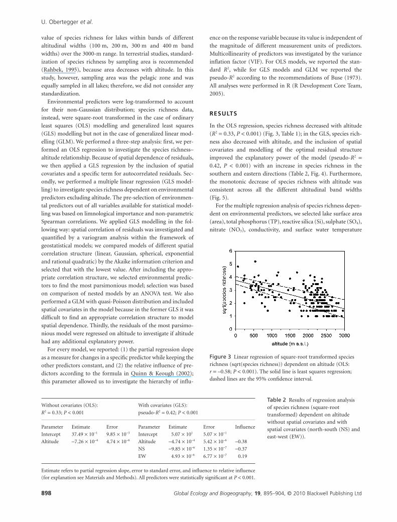
In the OLS regression, species richness decreased with altitude

(R2 = 0.33, P < 0.001) (Fig. 3, Table 1); in the GLS, species rich-

ness also decreased with altitude, and the inclusion of spatial

covariates and modelling of the optimal residual structure

improved the explanatory power of the model (pseudo-R2 =0.42, P < 0.001) with an increase in species richness in the

southern and eastern directions (Table 2, Fig. 4). Furthermore,

the monotonic decrease of species richness with altitude was

consistent across all the different altitudinal band widths

(Fig. 5).

For the multiple regression analysis of species richness depen-

dent on environmental predictors, we selected lake surface area

(area), total phosphorus (TP), reactive silica (Si), sulphate (SO4),

nitrate (NO3), conductivity, and surface water temperature

Figure 3 Linear regression of square-root transformed speciesrichness (sqrt(species richness)) dependent on altitude (OLS:r = –0.58; P < 0.001). The solid line is least squares regression;dashed lines are the 95% confidence interval.

Table 2 Results of regression analysisof species richness (square-roottransformed) dependent on altitudewithout spatial covariates and withspatial covariates (north-south (NS) andeast-west (EW)).

Without covariates (OLS):

R2 = 0.33; P < 0.001

With covariates (GLS):

pseudo-R2 = 0.42; P < 0.001

Parameter Estimate Error Parameter Estimate Error Influence

Intercept 37.49 ¥ 10-1 9.85 ¥ 10-3 Intercept 5.07 ¥ 101 5.07 ¥ 10-1

Altitude -7.26 ¥ 10-4 4.74 ¥ 10-6 Altitude -4.74 ¥ 10-4 5.42 ¥ 10-6 -0.38

NS -9.85 ¥ 10-6 1.35 ¥ 10-7 -0.37

EW 4.93 ¥ 10-6 6.77 ¥ 10-7 0.19

Estimate refers to partial regression slope, error to standard error, and influence to relative influence(for explanation see Materials and Methods). All predictors were statistically significant at P < 0.001.

U. Obertegger et al.

Global Ecology and Biogeography, 19, 895–904, © 2010 Blackwell Publishing Ltd898

Page 5

(temperature) based on limnological importance and non-

parametric Spearman correlations (Table 3). Area was a proxy

for habitat diversity, TP, Si and NO3 for productivity, SO4 for

human influence (atmospheric and terrestrial pollution), con-

ductivity for geology and temperature for the energy content of

water. In the multiple regression of species richness dependent

on environmental predictors, we first performed a GLS model

and considered autocorrelation of residuals; in this model, area,

Si, TP, NO3, SO4, temperature and conductivity were the most

important factors (GLS: pseudo-R2 = 0.49, P < 0.001) (Table 4).

Because species richness as count data can also be modelled by a

Poisson distribution, we subsequently performed a GLM and

included spatial covariates in the model. This new model better

accounted for the spatial structure of data and explained slightly

more variance (GLM: pseudo-R2 = 0.51, P < 0.001), but conduc-

tivity and SO4 were no longer significant and TP was borderline

(Table 4). The VIFs for this model were less than 10 for all

predictors and did not indicate multicollinearity among

variables.

The regression of residuals of the multiple regression models

(with and without spatial covariates) on altitude gave no signifi-

cant relationship (OLS: P > 0.05).

DISCUSSION

The understanding of the species richness–altitude relationship

is crucial for the development of a general theory on species

diversity (Rowe, 2009). In terrestrial studies, a linear decrease of

species richness with altitude is less common than a hump-

shaped pattern (Rahbek, 2005; Grytnes & McCain, 2007). This

pattern is seen as independent of sampling bias, while the linear

richness–altitude relationship is attributed to a decreased sam-

pling effort along altitude or to a truncated altitudinal gradient

(Rahbek, 2005; Nogués-Bravo et al., 2008). In the few aquatic

studies, however, species richness–altitude relationships tend to

show a monotonic decrease (Jones et al., 2003; Jacobsen, 2004;

Fontaneto & Ricci, 2006; Jankowski & Weyhenmeyer, 2006;

Hessen et al., 2007). Besides source–sink and rescue effects that

can inflate the estimate of species richness (Jones et al., 2003;

Grytnes & McCain, 2007), aquatic studies that show nonlinear

species richness–altitude patterns (Nyman et al., 2005; Jan-

kowski & Weyhenmeyer, 2006; Li et al., 2009) may also be biased

by unconsidered broad latitudinal and longitudinal gradients. In

fact, Rahbek (2005) points out that in studies covering extensive

geographical ranges, species richness along altitudinal gradients

is influenced by the different impact of historical and ecological

mechanisms along large latitudinal and longitudinal gradients.

Our study, conducted over a narrow geographical extent,

demonstrated that rotifer species richness decreased linearly

with altitude on a continuous scale. While Rahbek (2005)

underlines that monotonic decreasing patterns are rare when

considering altitudinal bands, in our study a linear pattern also

prevailed within altitudinal bands of different widths. We

suggest that this consistency across different scales further cor-

roborates the goodness of fit of the linear shape. In addition, the

inclusion of spatial covariates in the species richness–altitude

relationship improved the fit of the model (R2 = 0.33 versus

pseudo-R2 = 0.42). In fact, models that include spatial autocor-

relation have a better predictive power than models without it

because autocorrelation accounts for variance in species rich-

ness data (Currie, 2007).

But what does the geographic variable ‘altitude’ actually stand

for in relation to rotifer species richness? Recent research has

shown that altitudinal gradients cannot be attributed to a simple

universal explanation (Rowe, 2009). Based on multivariate

regressions (GLS and GLM), we discussed the importance of

environmental predictors and focused on the GLM because it

was the most appropriate one with respect to spatial dependence

of data. When excluding altitude as an environmental predictor,

we could show that area, Si, temperature and TP had a positive

effect on species richness, while NO3 had a negative one. In

Figure 4 Rotifer species richness in sampled sites: the diameterof closed circles corresponds to different classes of speciesrichness.

Figure 5 Rotifer species richness at different altitudinalresolutions. The range of altitudinal bands differs: (a) 100 mrange; (b) 200 m range; (c) 300 m range; (d) 400 m range (forexplanations see Materials and Methods).

Rotifer species richness in the Alps

Global Ecology and Biogeography, 19, 895–904, © 2010 Blackwell Publishing Ltd 899

Page 6

Tab

le3

Non

para

met

ric

Spea

rman

corr

elat

ion

ofen

viro

nm

enta

lvar

iabl

es:t

he

upp

erse

ctio

ngi

ves

sign

ifica

nce

,th

elo

wer

sect

ion

give

sco

rrel

atio

n;m

issi

ng

valu

esre

fer

ton

on-s

ign

ifica

nt

corr

elat

ion

san

d/or

corr

elat

ion

s<

0.20

.

Alt

iA

rea

Dep

thSR

PT

PN

H4

NO

3D

INSi

SO4

Cl

Ca

Mg

Na

KpH

Alk

Con

dTe

mp

NS

EW

Alt

i**

***

***

***

***

***

***

***

***

***

***

***

***

***

***

***

***

***

Are

a-0

.49

***

***

***

***

***

***

***

***

***

****

***

***

***

***

***

Dep

th-0

.25

0.72

***

***

***

***

***

SRP

-0.4

8**

***

***

***

***

***

***

***

TP

-0.4

60.

50**

***

***

***

***

***

***

***

***

***

***

NH

4-0

.25

0.40

****

***

***

***

***

***

***

***

***

***

NO

3-0

.35

0.41

0.32

0.22

***

***

***

***

***

***

***

****

***

*

DIN

-0.3

60.

420.

330.

290.

99**

***

***

***

***

***

****

***

*

Si-0

.54

0.41

0.29

0.45

0.21

0.23

0.21

***

***

***

***

SO4

0.20

0.26

0.31

0.32

***

***

***

***

***

***

***

***

**

Cl

-0.5

90.

310.

350.

520.

470.

280.

310.

300.

39**

***

***

***

***

***

***

***

***

*

Ca

-0.5

00.

320.

200.

260.

240.

290.

290.

570.

48**

***

***

***

***

***

***

*

Mg

-0.4

10.

250.

280.

300.

280.

290.

580.

480.

88**

***

***

***

***

***

*

Na

-0.5

50.

260.

340.

530.

320.

520.

530.

640.

450.

38**

***

***

***

***

*

K-0

.20

0.21

0.36

0.33

0.26

0.26

0.68

0.57

0.44

0.45

0.55

***

***

***

**

pH-0

.33

0.20

0.35

0.31

0.83

0.78

0.33

***

***

***

***

Alk

-0.5

70.

310.

240.

300.

200.

210.

210.

340.

480.

920.

800.

390.

340.

87**

***

***

***

*

Con

d-0

.50

0.34

0.28

0.28

0.32

0.32

0.62

0.51

0.99

0.93

0.47

0.48

0.82

0.88

***

**

Tem

p-0

.59

0.22

0.33

0.45

0.31

0.23

0.53

0.44

0.45

0.45

0.22

0.33

0.47

0.44

***

NS

-0.2

4-0

.30

-0.2

10.

250.

25**

*

EW

0.54

-0.4

2-0

.32

-0.4

6-0

.24

-0.2

8-0

.30

-0.5

9-0

.33

-0.2

5-0

.26

-0.3

00.

32

Alt

iis

alti

tude

,SR

Pis

solu

ble

reac

tive

phos

phat

e,D

INis

tota

ldis

solv

edin

orga

nic

nit

roge

n,A

lkis

alka

linit

y,C

ond

isco

ndu

ctiv

ity,

and

Tem

pis

tem

per

atu

re.

**P

<0.

01;*

**P

<0.

001.

U. Obertegger et al.

Global Ecology and Biogeography, 19, 895–904, © 2010 Blackwell Publishing Ltd900

Page 7

addition, the substitution of altitude by environmental predic-

tors explained more variance than altitude alone, and altitude

per se could not further account for the unexplained variation.

Therefore, we suggest that these combined predictors suffi-

ciently covered the effect of altitude on rotifer species richness.

Traditionally, the influence of area on species richness has

been explained by the theory of island biogeography (Mac-

Arthur & Wilson, 1967) or by the habitat diversity hypothesis

(Williams, 1964). However, these concepts are not mutually

exclusive, and theoretically they even seem to be complementary

because area and habitat diversity are correlated (Kallimanis

et al. 2008 and references therein). In our study, area was the

most influential predictor on species richness. We suggest that

lakes with larger area both sustained more vertical and horizon-

tal niches, offering greater habitat diversity, and had a lower

extinction and higher immigration rate than smaller lakes. Ver-

tical and horizontal niches are defined by physical, chemical and

biological parameters. As a consequence, habitat diversity

cannot be easily distinguished from other related factors

(Hessen et al., 2006). In fact, it was not surprising that area was

the predictor with the greatest effect on species richness because

it covers many different aspects of lake morphology.

Silica is an essential nutrient for siliceous algal species, pre-

dominantly diatoms and chrysophytes, and can limit growth

with concentrations below 0.5 mg l-1 (Parker et al., 2008). In this

way, silica influences algal productivity and succession and can

play an important role in rotifer species richness by determining

food composition (Swadling et al., 2000). Therefore, it was

expected that an environmental parameter related to nutrition

and productivity would score highly within the hierarchy of

predictor influence.

Temperature influences all metabolic functions and is a major

force in structuring communities (Litchman & Klausmeier,

2008) and in determining species diversity (Allen et al., 2002).

Our study also evidenced the positive effect of temperature on

species richness, but surprisingly, temperature scored third

within the hierarchy of effects. We attributed this to the represen-

tation of the temperature gradient by a single value (i.e. surface

water temperature). While surface water temperature could only

partially reflect the environmental temperature to which species

were exposed, it nevertheless determined the maximum tem-

perature present. In fact, surface water temperature is a good

surrogate for the actual input of energy (Hessen et al., 2007).

TP is a proxy for lake primary production (Hessen et al., 2006;

Barnett & Beisner, 2007). However, Jones et al. (2003) and

Barnett & Beisner (2007) note that this parameter is a poor

predictor for species richness. We also found that TP was only

marginally significant. It seems that this predictor is more

closely related to functional than taxonomic diversity (Barnett &

Beisner, 2007), an issue that would require further investigation.

In temperate lakes, phosphorus and silica are the most

common limiting nutrients, while nitrogen is limiting only

when the N:P ratio is < 16 (Lampert & Sommer, 2007). This was

the case in 29% of our lakes, and we expected a positive influ-

ence of nitrates on species richness; contrarily, it had a negative

effect. While high concentrations of nitrates can cause a wide

range of problems including loss of biodiversity (Carpenter

et al., 1998), in all our lakes, concentrations of nitrates were

much lower than the 10 mg NO3 l-1 threshold for potential

toxicity to aquatic organisms (Camargo & Alonso, 2006). Non-

point pollution from agriculture and urban activity, including

industry and transport, is a major source of nitrogen for fresh

water (Camargo & Alonso, 2006). The same sources also trans-

port many complex, ill-defined chemicals (e.g. pharmaceuticals,

pesticides, fertilizers and their metabolites) (Sumpter, 2009).

Rotifers are sensitive to pollutants, and this determines their use

as indicators of trophic conditions and test organisms in toxicity

assays (Sládecek, 1983). We suggest that the negative effect of

nitrates on species richness could be related to unmeasured

co-occurring pollutants, and consequently this predictor

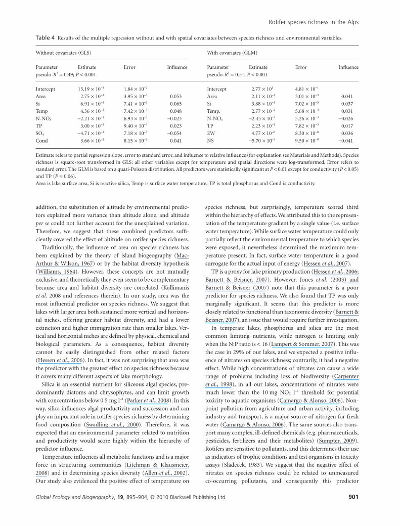
Table 4 Results of the multiple regression without and with spatial covariates between species richness and environmental variables.

Without covariates (GLS) With covariates (GLM)

Parameter Estimate Error Influence Parameter Estimate Error Influence

pseudo-R2 = 0.49; P < 0.001 pseudo-R2 = 0.51; P < 0.001

Intercept 15.19 ¥ 10-1 1.84 ¥ 10-2 Intercept 2.77 ¥ 101 4.81 ¥ 10-1

Area 2.75 ¥ 10-1 3.95 ¥ 10-3 0.053 Area 2.11 ¥ 10-1 3.01 ¥ 10-3 0.041

Si 6.91 ¥ 10-1 7.41 ¥ 10-3 0.065 Si 3.88 ¥ 10-1 7.02 ¥ 10-3 0.037

Temp 4.36 ¥ 10-2 7.42 ¥ 10-4 0.048 Temp. 2.77 ¥ 10-2 5.68 ¥ 10-4 0.031

N-NO3 -2.21 ¥ 10-1 6.93 ¥ 10-3 -0.023 N-NO3 -2.45 ¥ 10-1 5.26 ¥ 10-3 -0.026

TP 3.00 ¥ 10-1 9.40 ¥ 10-3 0.023 TP 2.23 ¥ 10-1 7.82 ¥ 10-3 0.017

SO4 -4.71 ¥ 10-1 7.18 ¥ 10-3 -0.054 EW 4.77 ¥ 10-6 8.30 ¥ 10-8 0.036

Cond 3.66 ¥ 10-1 8.15 ¥ 10-3 0.041 NS -5.70 ¥ 10-4 9.50 ¥ 10-8 -0.041

Estimate refers to partial regression slope, error to standard error, and influence to relative influence (for explanation see Materials and Methods). Speciesrichness is square-root transformed in GLS; all other variables except for temperature and spatial directions were log-transformed. Error refers tostandard error. The GLM is based on a quasi-Poisson distribution. All predictors were statistically significant at P < 0.01 except for conductivity (P < 0.05)and TP (P = 0.06).Area is lake surface area, Si is reactive silica, Temp is surface water temperature, TP is total phosphorus and Cond is conductivity.

Rotifer species richness in the Alps

Global Ecology and Biogeography, 19, 895–904, © 2010 Blackwell Publishing Ltd 901

Page 8

seemed to be related to human influence instead of

productivity.

Apart from environmental predictors, spatial covariates were

important factors for the species richness–environment rela-

tionship. In fact, the spatial structure of environmental data has

to be taken into account even if it is not an easy task to find the

most appropriate model (Beguería & Pueyo, 2009). In the

species richness–altitude model as well as in the species

richness–environment model, spatial covariates had the same

effect on species richness. We related the increase in species

richness along the easterly and southerly directions (Fig. 3) to

the geological heterogeneity of our study area, where very dif-

ferent geological formations can be found over short distances

(Fig. 6). While with the inclusion of covariates in the linear

regression the fit was markedly improved, in the multiple regres-

sion the variance increased only slightly (GLM: pseudo-R2 =0.49 versus 0.51) but led to the non-significance of conductivity

and sulphates. This comparison of different statistical ap-

proaches revealed the spatial structure of our data: we suggest

that conductivity and sulphates had a strong spatial component

that could be completely described by geographical directions.

In our study region, lake conductivity reflected geological origin

with metamorphic bedrock more common in the northern part

and easily weathered sedimentary bedrock more common in the

southern part of the region (Fig. 6). Sulphate was also related to

geographical directions even if it was regarded as a proxy for

human influence. However, we cannot exclude some overlap of

human influence within spatial dependence. Other parameters

linked to weathering of the bedrock, such as silica, might also

have a spatial component that could not, however, be completely

described by covariates.

Interestingly, five high-altitude lakes (Finailsee, Hunger-

schartensee, Langsee-Ulten, Kleiner Plombodensee, Schwarzsee-

Ulten) on metamorphic bedrock had higher than expected

sulphate (range 50–95 mg l-1 SO4) and conductivity (range 132–

233 mS cm-1) values (Fig. 6). While alpine lakes were once con-

sidered pristine environments, a recent review on European

mountain lakes shows them to be impacted by atmospheric

deposition and global warming (Battarbee et al., 2009). The

melting of ice and rock glaciers leads to an increase of conduc-

tivity due to the release of solutes and pollutants such as sul-

phate, nickel and manganese previously immobilized in the ice

(e.g. Thies et al., 2007). We suggest that these extraordinarily

high values of conductivity and sulphate for lakes located on

metamorphic bedrock could be an early warning sign of the

impact of melting ice on high-altitude aquatic systems.

By our model, we explained 51% of the variability of species

richness using environmental predictors and spatial covariates.

While environmental predictors of the species richness–altitude

pattern were related to specific key factors such as habitat diver-

sity, productivity, heat content and human influence, spatial

covariates were linked to the geologically heterogeneous terri-

tory. Our study underlined how including both environmental

and spatial predictors can enhance hypothesis-driven consider-

ations on species richness. Further unexplained variability of

species richness might be attributed to unconsidered factors

such as inter- and intraspecific competition for food sources

(Walz, 1995), hydrology (Soranno et al., 1999; Obertegger et al.,

2007) and dispersal (Swadling et al., 2000).

The linear decrease of species richness along the altitudinal

gradient was successfully captured by the interplay of habitat

diversity, productivity, heat content and human influence. But

why do terrestrial studies mainly show a hump-shaped pattern

of species richness while aquatic studies tend to show a linear

pattern? The inclusion of anthropogenically disturbed habitats

can cause a hump-shaped pattern (Nogués-Bravo et al., 2008),

and we argue that this may not completely apply to aquatic

systems. Recent improvements in water quality, especially in

temperate lowland lakes, while not limiting non-point sources,

have greatly reduced direct pollution (Søndergaard & Jeppesen,

2007). Moreover, precipitation (Gotelli et al., 2009) or water

availability (Grytnes & McCain, 2007) are very decisive in con-

junction with temperature for the unimodal species richness

pattern. However, aquatic systems – to be considered as such –

must retain their aquatic status, along with their main physical

properties related to water. Obviously, aquatic systems are also

subject to change, but in contrast to terrestrial ones, water pro-

vides a relatively stable set-up of environmental conditions in

which biotic interactions take place (Reynolds, 1998; Lampert

& Sommer, 2007).These characteristics of freshwater ecosys-

tems may ultimately distinguish them from their terrestrial

counterparts with regards to the species richness–altitude rela-

tionship. We argue that the factors determining species

richness–altitude patterns tend to be the same in terrestrial and

aquatic habitats, but the greater environmental stability of

Figure 6 Conductivity (mS cm-1) in sampled sites with theunderlying bedrock: the diameter of closed circles corresponds todifferent classes of conductivity. Lakes with unexpectedly highsulphate and conductivity values are circled.

U. Obertegger et al.

Global Ecology and Biogeography, 19, 895–904, © 2010 Blackwell Publishing Ltd902

Page 9

aquatic systems seems to lead to linear instead of hump-shaped

patterns.

ACKNOWLEDGEMENTS

U.O. is supported by post-doc grant CERCA (Province of

Trento, Italy). This work was carried out within the research

activity funded by IASMA and an ECOPLAN Research Grant

(Province of Trento, Italy). We thank Vigilio Pinamonti, Gino

Leonardi and Franz Obertegger for help with sampling, Gio-

vanna Pellegrini for access to some unpublished data and Fabio

Zottele for statistical advice and the site map. We also thank

David Currie, Patricia Soranno and an anonymous referee for

suggestions that substantially improved this manuscript.

REFERENCES

Allen, A.P., Brown, J.H. & Gillooly, J.F. (2002) Global biodiver-

sity, biochemical kinetics, and the energetic-equivalence rule.

Science, 297, 1545–1548.

Barnett, A. & Beisner, B.E. (2007) Zooplankton biodiversity and

lake trophic state: explanations invoking resource abundance

and distribution. Ecology, 88, 1675–1686.

Battarbee, R.W., Kernan, M. & Rose, N. (2009) Threatened and

stressed mountain lakes of Europe: assessment and progress.

Aquatic Ecosystem Health and Management, 12, 118–128.

Bêche, L.A. & Statzner, B. (2009) Richness gradients of stream

invertebrates across the USA: taxonomy- and trait-based

approaches. Biodiversity and Conservation, 18, 3909–3930.

Beguería, S. & Pueyo, Y. (2009) A comparison of simultaneous

autoregressive and generalized least squares models for

dealing with spatial autocorrelation. Global Ecology and Bio-

geography, 18, 273–279.

Buse, A. (1973) Goodness of fit in generalized least squares

estimation. The American Statistician, 27, 106–108.

Camargo, J.A. & Alonso, Á. (2006) Ecological and toxicological

effects of inorganic nitrogen pollution in aquatic ecosystems:

a global assessment. Environment International, 32, 831–849.

Cantonati, M. & Lazzara, M. (2006) High mountain lakes in the

Avisio River watershed (east Trentino). Natural History

Museum of Trento, Trento, Italy (in Italian).

Cantonati, M., Tolotti, M. & Lazzara, M. (2002) Lakes in the

Adamello-Brenta Natural Park. Natural History Museum of

Trento, Trento, Italy (in Italian).

Carpenter, S.R., Caraco, N.F., Correll, D.L., Howarth, R.W.,

Sharpley, A.N. & Smith, V.H. (1998) Nonpoint pollution of

surface waters with phosphorus and nitrogen. Ecological

Applications, 8, 559–568.

Colwell, R.K. & Lees, D.C. (2000) The mid-domain effect: geo-

metric constraints on the geography of species richness.

Trends in Ecology and Evolution, 15, 70–76.

Currie, D.J. (2007) Disentangling the roles of environment and

space in ecology. Journal of Biogeography, 34, 2009–2011.

Currie, D.J. & Kerr, J.T. (2008) Tests of the mid-domain hypoth-

esis: a review of the evidence. Ecological Monographs, 78, 3–18.

Davies, R.G., Orme, C.D.L., Webster, A.J., Jones, K.E., Blackburn,

T.M. & Gaston, K.J. (2007) Environmental predictors of global

parrot (Aves: Psittaciformes) species richness and phylogenetic

diversity. Global Ecology and Biogeography, 16, 220–233.

Fontaneto, D. & Ricci, C. (2006) Spatial gradients in species

diversity of microscopic animals: the case of bdelloid rotifers

at high altitude. Journal of Biogeography, 33, 1305–1313.

Gotelli, N.J., Anderson, M.J., Arita, H.T. et al. (2009) Patterns

and causes of species richness: a general simulation model for

macroecology. Ecology Letters, 12, 873–886.

Grytnes, J.A. & McCain, C.M. (2007) Elevational trends in

biodiversity. Encyclopedia of biodiversity (ed. by S.A. Levin),

pp. 1–8. Elsevier Inc., New York.

Grytnes, J.A., Heegaard, E. & Ihlen, P.G. (2006) Species richness

of vascular plants, bryophytes, and lichens along an altitudinal

gradient in western Norway. Acta Oecologica, 29, 241–246.

Hessen, D.O., Faafeng, B.A., Smith, V.H., Bakkestuen, V. &

Walseng, B. (2006) Extrinsic and intrinsic controls of zoop-

lankton diversity in lakes. Ecology, 87, 433–443.

Hessen, D.O., Bakkestuen, V. & Walseng, B. (2007) Energy input

and zooplankton species richness. Ecography, 30, 749–758.

Hubbell, S.P. (2001) The unified neutral theory of biodiversity and

biogeography. Princeton University Press, Princeton, NJ.

IASMA (1996–2000) Annual reports on the limnological charac-

teristics of Trentino lakes. Istituto Agrario di San Michele

all’Adige, Trento (in Italian).

Jacobsen, D. (2004) Contrasting patterns in local and zonal

family richness of stream invertebrates along an Andean alti-

tudinal gradient. Freshwater Biology, 49, 1293–1305.

Jankowski, T. & Weyhenmeyer, G.A. (2006) The role of spatial

scale and area in determining richness–altitude gradients in

Swedish lake phytoplankton communities. Oikos, 115, 433–

442.

Jersabek, C.D. (1995) Distribution and ecology of rotifer com-

munities in high-altitude alpine sites – a multivariate

approach. Hydrobiologia, 313, 75–89.

Jones, J.I., Li, W. & Maberly, S.C. (2003) Area, altitude and

aquatic plant diversity. Ecography, 26, 411–420.

Kallimanis, A.S., Mazaris, A.D., Tzanopoulos, J., Halley, J.M.,

Pantis, J.D. & Sgardelis, S.P. (2008) How does habitat diversity

affect the species–area relationship? Global Ecology and Bioge-

ography, 17, 532–538.

Kluge, J., Kessler, M. & Dunn, R.R. (2006) What drives eleva-

tional patterns of biodiversity? A test of geometric constraints,

climate, and species pool effects for pteridophytes on an eleva-

tional gradient in Costa Rica. Global Ecology and Biogeogra-

phy, 15, 358–371.

Körner, C. (2007) The use of ‘altitude’ in ecological research.

Trends in Ecology and Evolution, 22, 569–574.

Lampert, W. & Sommer, U. (2007) Limnoecology. The ecology of

lakes and streams. Oxford University Press, Oxford.

Li, J., He, Q., Hua, X., Zhou, J., Xu, H., Chen, J. & Fu, C. (2009)

Climate and history explain the species richness peak at mid-

elevation for Schizothorax fishes (Cypriniformes: Cyprinidae)

distributed in the Tibetan Plateau and its adjacent regions.

Global Ecology and Biogeography, 18, 264–272.

Rotifer species richness in the Alps

Global Ecology and Biogeography, 19, 895–904, © 2010 Blackwell Publishing Ltd 903

Page 10

Litchman, E. & Klausmeier, C.A. (2008) Trait-based community

ecology of phytoplankton. Annual Review of Ecology, Evolu-

tion, and Systematics, 39, 615–639.

MacArthur, R.H. & Wilson, E.O. (1967) The theory of island

biogeography. Princeton University Press, Princeton, NJ.

McCain, C.M. (2007) Area and mammalian elevational diver-

sity. Ecology, 88, 76–86.

Nogués-Bravo, D., Araùjo, M.B., Romdal, T. & Rahbek, C.

(2008) Scale effects and human impact on the elevational

species richness gradients. Nature, 453, 216–220.

Nyman, M., Korhola, A. & Brooks, S.J. (2005) The distribution

and diversity of Chironomidae (Insecta: Diptera) in western

Finnish Lapland, with special emphasis on shallow lakes.

Global Ecology and Biogeography, 14, 137–153.

Obertegger, U., Flaim, G., Braioni, M.G., Sommaruga, R.,

Corradini, F. & Borsato, A. (2007) Water residence time as a

driving force of zooplankton structure and succession.

Aquatic Sciences, 69, 575–583.

Obertegger, U., Thaler, B. & Flaim, G. (2008) Habitat constraints

of Synchaeta (Rotifera) in north Italian lakes (Trentino–South

Tyrol). Verhandlungen Internationale Vereinigung für Theore-

tische und Angewandte Limnologie, 30, 302–306.

Parker, B.R., Vinebrooke, R.D. & Schindler, D.W. (2008) Recent

climate extremes alter alpine lake ecosystems. Proceedings of

the National Academy of Sciences USA, 105, 12927–12931.

Quinn, G.P. & Keough, M.J. (2002) Experimental design and

data analysis for biologists. Cambridge University Press,

Cambridge.

R Development Core Team (2005) R: a language and environ-

ment for statistical computing. R Foundation for Statistical

Computing, Vienna. Available at: http://www.r-project.org/

(accessed 26 June 2009).

Rahbek, C. (1995) The elevational gradient of species richness –

a uniform pattern. Ecography, 18, 200–205.

Rahbek, C. (2005) The role of spatial scale and the perception of

large-scale species-richness patterns. Ecological Letters, 8, 224–

239.

Reynolds, C.S. (1998) The state of freshwater ecology. Freshwa-

ter Biology, 39, 741–753.

Rowe, R.J. (2009) Environmental and geometric drivers of small

mammal diversity along elevational gradients in Utah.

Ecography, 32, 411–422.

Salmaso, N. & Naselli-Flores, L. (1999) Studies on the zooplank-

ton of the deep subalpine Lake Garda. Journal of Limnology,

58, 66–76.

Scheffer, M. & van Geest, G.J. (2006) Small habitat size and

isolation can promote species richness: second-order effects

on biodiversity in shallow lakes and ponds. Oikos, 112, 227–

231.

Sládecek, V. (1983) Rotifers as indicators of water-quality.

Hydrobiologia, 100, 169–201.

Smith, K.F. & Brown, J.H. (2002) Patterns of diversity, depth

range and body size among pelagic fishes along a gradient of

depth. Global Ecology and Biogeography, 11, 313–322.

Søndergaard, M. & Jeppesen, E. (2007) Anthropogenic impacts

on lake and stream ecosystems, and approaches to restoration.

Journal of Applied Ecology, 44, 1089–1094.

Soranno, P.A., Webster, K.E., Riera, J.L., Kratz, T.K., Baron, J.S.,

Bukaveckas, P.A., Kling, G.W., White, D.S., Caine, N., Lathrop,

R.C. & Leavitt, P.R. (1999) Spatial variation among lakes

within landscapes: ecological organization along lake chains.

Ecosystems, 2, 395–410.

Sturm, R. (2007) Freshwater molluscs in mountain lakes of the

eastern Alps (Austria): relationship between environmental

variables and lake colonization. Journal of Limnology, 66, 160–

169.

Sumpter, J.P. (2009) Protecting aquatic organisms from chemi-

cals: the harsh realities. Philosophical Transactions of the Royal

Society A: Mathematical Physical and Engineering Sciences,

367, 3877–3894.

Swadling, K.M., Pienitz, R. & Nogrady, T. (2000) Zooplankton

community composition of lakes in the Yukon and Northwest

Territories (Canada): relationship to physical and chemical

limnology. Hydrobiologia, 431, 211–224.

Thies, H.J., Nickus, U., Mair, V., Tessadri, R., Tait, D., Thaler, B.

& Psenner, R. (2007) Unexpected response of high alpine lake

waters to climate warming. Environmental Science and Tech-

nology, 41, 7424–7429.

Walz, N. (1995) Rotifer populations in plankton communities:

energetics and life history strategies. Experientia, 51, 437–453.

Wiens, J.J. & Donoghue, M.J. (2004) Historical biogeography,

ecology and species richness. Trends in Ecology and Evolution,

19, 639–644.

Williams, C.B. (1964) Patterns in the balance of nature. Academic

Press, London.

BIOSKETCHES

Ulrike Obertegger is a post-doc fellow at the IASMA

Research and Innovation Centre, FEM, Trento. Her

main research interests are rotifer taxonomy, ecology

and distribution patterns, and in particular the role of

environmental factors that drive zooplankton

biodiversity at different scales. She also is a

mountaineer with a passion for high-altitude lake

sampling.

Bertha Thaler is a limnologist at the provincial

Environmental Protection Agency, Bozen. Her main

interests are lake monitoring and zooplankton ecology,

with particular emphasis on alpine lakes.

Giovanna Flaim is a limnologist at the IASMA

Research and Innovation Centre, FEM, Trento. Her

main interests are in ecosystem functioning and the

relation of abiotic and biotic factors to plankton

autecology.

Editor: Tim Blackburn

U. Obertegger et al.

Global Ecology and Biogeography, 19, 895–904, © 2010 Blackwell Publishing Ltd904