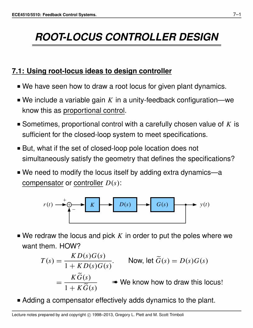
ECE4510/5510: Feedback Control Systems. 7–1 ROOT-LOCUS CONTROLLER DESIGN 7.1: Using root-locus ideas to design controller ■ We have seen how to draw a root locus for given plant dynamics. ■ We include a variable gain K in a unity-feedback configuration—we know this as proportional control. ■ Sometimes, proportional control with a carefully chosen value of K is sufficient for the closed-loop system to meet specifications. ■ But, what if the set of closed-loop pole location does not simultaneously satisfy the geometry that defines the specifications? ■ We need to modify the locus itself by adding extra dynamics—a compensator or controller D (s ): r (t ) y (t ) K G (s ) D(s ) ■ We redraw the locus and pick K in order to put the poles where we want them. HOW? T (s ) = KD (s ) G (s ) 1 + KD (s ) G (s ) . Now, let G (s ) = D (s ) G (s ) = K G (s ) 1 + K G (s ) ➠ We know how to draw this locus! ■ Adding a compensator effectively adds dynamics to the plant. Lecture notes prepared by and copyright c 1998–2013, Gregory L. Plett and M. Scott Trimboli

Welcome message from author
This document is posted to help you gain knowledge. Please leave a comment to let me know what you think about it! Share it to your friends and learn new things together.
Transcript
ECE4510/5510: Feedback Control Systems. 7–1
ROOT-LOCUS CONTROLLER DESIGN
7.1: Using root-locus ideas to design controller
! We have seen how to draw a root locus for given plant dynamics.
! We include a variable gain K in a unity-feedback configuration—weknow this as proportional control.
! Sometimes, proportional control with a carefully chosen value of K issufficient for the closed-loop system to meet specifications.
! But, what if the set of closed-loop pole location does notsimultaneously satisfy the geometry that defines the specifications?
! We need to modify the locus itself by adding extra dynamics—acompensator or controller D(s):
r (t) y(t)K G(s)D(s)
! We redraw the locus and pick K in order to put the poles where wewant them. HOW?
T (s) = K D(s)G(s)1 + K D(s)G(s)
. Now, let !G(s) = D(s)G(s)
= K !G(s)1 + K !G(s)
" We know how to draw this locus!
! Adding a compensator effectively adds dynamics to the plant.
Lecture notes prepared by and copyright c! 1998–2013, Gregory L. Plett and M. Scott Trimboli
ECE4510/ECE5510, ROOT-LOCUS CONTROLLER DESIGN 7–2
Adding a left-half-plane pole or zero
! What types of (1) compensation should we use, and (2) how do wefigure out where to put the additional dynamics?
! In ECE4510/5510, the methods we discuss are “science-inspired art.”
• We need to get a “feel” for how the root locus changes when polesand zeros are added, to understand what dynamics to use for D(s).
! In more advanced courses, we learn more powerful methods:
• In ECE5520, we learn how to put all closed-loop poles exactlywhere we want them (where do we want them?)
• In ECE5530, we learn how to find the optimal set of pole locations.
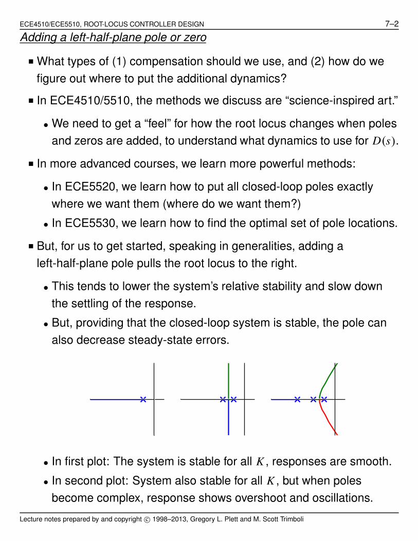
! But, for us to get started, speaking in generalities, adding aleft-half-plane pole pulls the root locus to the right.
• This tends to lower the system’s relative stability and slow downthe settling of the response.
• But, providing that the closed-loop system is stable, the pole canalso decrease steady-state errors.
• In first plot: The system is stable for all K , responses are smooth.
• In second plot: System also stable for all K , but when polesbecome complex, response shows overshoot and oscillations.
Lecture notes prepared by and copyright c! 1998–2013, Gregory L. Plett and M. Scott Trimboli

ECE4510/ECE5510, ROOT-LOCUS CONTROLLER DESIGN 7–3
• In third plot: The system is stable only for small K , and oscillationsincrease as the poles approach the imaginary axis.
• But, steady-state error improves from left to right (assuming theclosed-loop system is stable).
! Again, generally speaking, adding a left-half-plane zero pulls the rootlocus to the left.
• This tends to make the system more stable, and speed up thesettling of the response.
• Physically, a zero adds derivative control to the system, introducinganticipation into the system, speeding up transient response.
• However, steady-state errors can get worse.
• In first plot: System is stable only for small K , and oscillates aspoles approach imaginary axis.
• In second plot: System is stable for all K , but still oscillates.
• In third and fourth plots: More stable, less oscillation.
• But, steady-state error degrades from left to right.
! Can’t physically add a zero without a pole: Must put pole very far leftin s-plane so we don’t deteriorate desired impact of zero.
Lecture notes prepared by and copyright c! 1998–2013, Gregory L. Plett and M. Scott Trimboli
ECE4510/ECE5510, ROOT-LOCUS CONTROLLER DESIGN 7–4
7.2: Reducing steady-state error
! We have a number of options available to us if we wish to reducesteady-state error.
1) Proportional feedback
D(s) = 1. u(t) = K e(t)
T (s) = K G(s)1 + K G(s)
.
! Same as what we have already looked at.
! Controller consists of only a “gain knob.”
• Increasing gain K often reduces steady-state error, but candegrade transient response.
• We have to take the locus “as given” since we have no extradynamics to modify it.
• Can’t independently choose steady-state error and transientresponse. Can design for one or other, not both.
! Usually a very limited approach, but a good place to start.
2) Integral feedback
D(s) = 1TI s
u(t) = KTI
" t
0e(! ) d!
T (s) =KTI
G(s)s
1 + KTI
G(s)s
.
! Usually used to reduce/eliminate steady-state error. i.e., if e(t)constant, u(t) will become very large and hopefully correct the error.
! Ideally, we would like no error, ess = 0. (Maybe 1 % to 2 % in reality)
Lecture notes prepared by and copyright c! 1998–2013, Gregory L. Plett and M. Scott Trimboli
ECE4510/ECE5510, ROOT-LOCUS CONTROLLER DESIGN 7–5
ANALYSIS: For a unity-feedback control system, the steady-state error toa unit-step input is:
ess = 11 + K D(0)G(0)
.
! If we make D(s) = 1TI s
, then as s " 0, D(s) " #
ess " 11 + # = 0.
! Adding the integrator into the compensator has reduced error from1
1 + K pto zero for systems that do not have any free integrators.
! Adding the integrator increases the system type, but as steady-stateresponse improves, transient response often degrades.
EXAMPLE: G(s) = 1(s + a)(s + b)
, a > b > 0.
! Proportional feedback, D(s) = 1, G(0) = 1ab
, ess = 11 + K
ab
.
$a $b
I(s)
R(s)
! We can make ess small bymaking K very large, but thisoften leads to poorly-dampedbehavior and often requiresexcessively large actuators.
! Integral feedback, D(s) = 1TI s
, ess = 0.
Lecture notes prepared by and copyright c! 1998–2013, Gregory L. Plett and M. Scott Trimboli

ECE4510/ECE5510, ROOT-LOCUS CONTROLLER DESIGN 7–6
$a $b
I(s)
R(s)
! Increasing K to increase thespeed of response pushesthe pole toward theimaginary axis " oscillatory.
3) Proportional-integral (PI) control
! Now, D(s) = K#
1 + 1TI s
$= K
#s + (1/TI )
s
$. Both a pole and a zero.
$a $b
I(s)
R(s)
! Combination of proportionaland integral (PI) solves manyof the problems with just (I)integral.
4) Phase-lag control
! The integrator in PI control can cause some practical problems; e.g.,“integrator windup” due to actuator saturation.
! PI control is often approximated by “lag control.”
D(s) = (s $ z0)
(s $ p0), |p0| < |z0|.
That is, the pole is closer to the origin than the zero.
! Because |z0| > |p0|, the phase " added to the open-loop transferfunction is negative. . . “phase lag”
! Pole often placed very close to zero. e.g., p0 % 0.01.
Lecture notes prepared by and copyright c! 1998–2013, Gregory L. Plett and M. Scott Trimboli
ECE4510/ECE5510, ROOT-LOCUS CONTROLLER DESIGN 7–7
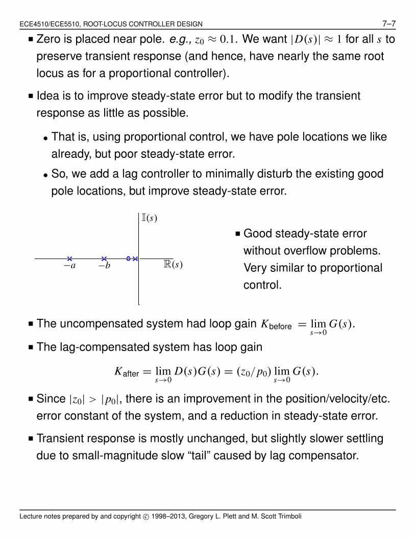
! Zero is placed near pole. e.g., z0 % 0.1. We want |D(s)| % 1 for all s topreserve transient response (and hence, have nearly the same rootlocus as for a proportional controller).
! Idea is to improve steady-state error but to modify the transientresponse as little as possible.
• That is, using proportional control, we have pole locations we likealready, but poor steady-state error.
• So, we add a lag controller to minimally disturb the existing goodpole locations, but improve steady-state error.
$a $b
I(s)
R(s)
! Good steady-state errorwithout overflow problems.Very similar to proportionalcontrol.
! The uncompensated system had loop gain Kbefore = lims"0
G(s).
! The lag-compensated system has loop gain
Kafter = lims"0
D(s)G(s) = (z0/p0) lims"0
G(s).
! Since |z0| > |p0|, there is an improvement in the position/velocity/etc.error constant of the system, and a reduction in steady-state error.
! Transient response is mostly unchanged, but slightly slower settlingdue to small-magnitude slow “tail” caused by lag compensator.
Lecture notes prepared by and copyright c! 1998–2013, Gregory L. Plett and M. Scott Trimboli
ECE4510/ECE5510, ROOT-LOCUS CONTROLLER DESIGN 7–8
7.3: Improving transient response
! We have a number of options available to us if we wish to improvetransient response
1) Proportional feedback
! Again, we could use a proportional feedback controller.
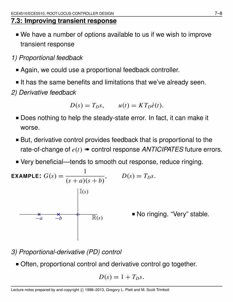
! It has the same benefits and limitations that we’ve already seen.2) Derivative feedback
D(s) = TDs, u(t) = K TDe(t).
! Does nothing to help the steady-state error. In fact, it can make itworse.
! But, derivative control provides feedback that is proportional to therate-of-change of e(t) " control response ANTICIPATES future errors.
! Very beneficial—tends to smooth out response, reduce ringing.
EXAMPLE: G(s) = 1(s + a)(s + b)
, D(s) = TDs.
$a $b
I(s)
R(s)! No ringing. “Very” stable.
3) Proportional-derivative (PD) control
! Often, proportional control and derivative control go together.
D(s) = 1 + TDs.
Lecture notes prepared by and copyright c! 1998–2013, Gregory L. Plett and M. Scott Trimboli

ECE4510/ECE5510, ROOT-LOCUS CONTROLLER DESIGN 7–9
$a $b
I(s)
R(s)
! No more zero at s = 0.
! Therefore better steady-stateresponse.
4) Phase-lead control
! Derivative magnifies sensor noise.
! Instead of D-control or PD-control use “lead control.”
D(s) = (s $ z0)
(s $ p0), |z0| < |p0|.
That is, the zero is closer to the origin than the pole.
! Same form as lag control, but with different intent:
• Lag control does not change locus much since p0 % z0 % 0.Instead, lag control improves steady-state error.
• Lead control DOES change locus. Pole and zero locations chosenso that locus will pass through some desired point s = s1.
DESIGN METHOD I: Sometimes, we can be successful by choosing thevalue of z0 to cancel a stable pole in the plant.
! Then, we solve for K and p0 such that
[1 + K D(s)G(s)|s=s1 = 0.
! That is, we force one closed-loop pole to be at s = s1.
! This does not ensure that other poles do anything reasonable, so wemust always test design.
Lecture notes prepared by and copyright c! 1998–2013, Gregory L. Plett and M. Scott Trimboli
ECE4510/ECE5510, ROOT-LOCUS CONTROLLER DESIGN 7–10
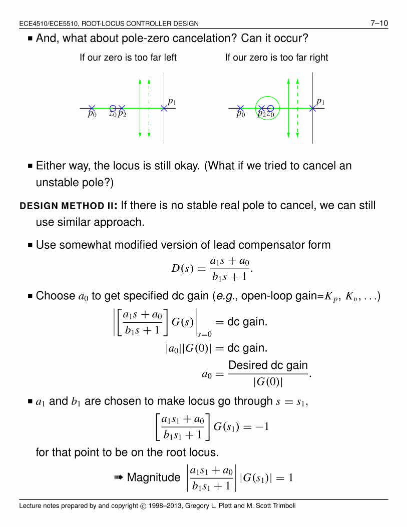
! And, what about pole-zero cancelation? Can it occur?
If our zero is too far left If our zero is too far right
p1
p2z0p0
p1
p2z0p0
! Either way, the locus is still okay. (What if we tried to cancel anunstable pole?)
DESIGN METHOD II: If there is no stable real pole to cancel, we can stilluse similar approach.
! Use somewhat modified version of lead compensator form
D(s) = a1s + a0
b1s + 1.
! Choose a0 to get specified dc gain (e.g., open-loop gain=K p, Kv, . . .)%%%%
#a1s + a0
b1s + 1
$G(s)
%%%%s=0
= dc gain.
|a0||G(0)| = dc gain.
a0 = Desired dc gain|G(0)| .
! a1 and b1 are chosen to make locus go through s = s1,#a1s1 + a0
b1s1 + 1
$G(s1) = $1
for that point to be on the root locus.
" Magnitude%%%%a1s1 + a0
b1s1 + 1
%%%% |G(s1)| = 1
Lecture notes prepared by and copyright c! 1998–2013, Gregory L. Plett and M. Scott Trimboli

ECE4510/ECE5510, ROOT-LOCUS CONTROLLER DESIGN 7–11
" Phase &#
a1s1 + a0
b1s1 + 1
$+ & G(s1) = 180'.
(math happens)
a1 = sin(#) + a0|G(s1)| sin(# $ $)
|s1||G(s1)| sin($)
b1 = sin(# + $) + a0|G(s1)| sin(#)
$|s1| sin($)
&''(
'')
s1 = |s1|e j#
G(s1) = |G(s1)|e j$.
5) Proportional-integral-derivative (PID) control
! There is a similar design procedure for PID control:
D(s) = K#
1 + 1TI s
+ TDs$
= K p + K I
s+ Kds.
! Compute: K p = $ sin(# + $)
|G(s1)| sin(#)$ 2K I cos#
|s1|! Compute: K D = sin($)
|s1||G(s1)| sin(#)+ K I
|s1|2, where s1 = |s1|e j# and
G(s1) = |G(s1)|e j$ for both cases.
! TI chosen to match some design criteria. e.g., steady-state error.
! Convert to first form via K = K p; TI = K/K I ; TD = Kd/K .
6) Lead-lag control
! If we must satisfy both a transient and steady-state spec:
1. Design a lead controller to meet transient spec first;2. Include lead controller with plant after its design is final;3. Design a lag controller (where “plant” = actual plant and lead
controller combined) to meet steady-state spec.
Lecture notes prepared by and copyright c! 1998–2013, Gregory L. Plett and M. Scott Trimboli
ECE4510/ECE5510, ROOT-LOCUS CONTROLLER DESIGN 7–12
7.4: Examples (a)
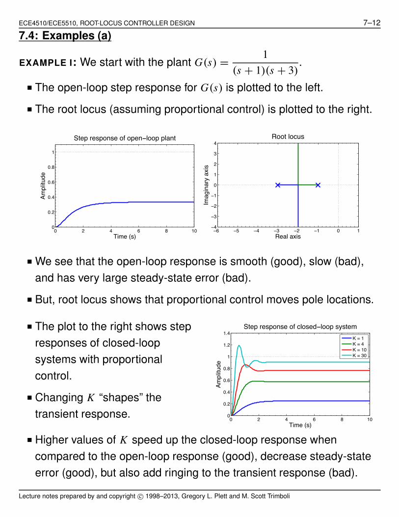
EXAMPLE I: We start with the plant G(s) = 1(s + 1)(s + 3)
.
! The open-loop step response for G(s) is plotted to the left.
! The root locus (assuming proportional control) is plotted to the right.
0 2 4 6 8 100
0.2
0.4
0.6
0.8
1
Time (s)
Ampl
itude
Step response of open−loop plant
−6 −5 −4 −3 −2 −1 0 1−4
−3
−2
−1
0
1
2
3
4
Real axis
Imag
inar
y ax
is
Root locus
! We see that the open-loop response is smooth (good), slow (bad),and has very large steady-state error (bad).
! But, root locus shows that proportional control moves pole locations.
! The plot to the right shows stepresponses of closed-loopsystems with proportionalcontrol.
! Changing K “shapes” thetransient response.
0 2 4 6 8 100
0.2
0.4
0.6
0.8
1
1.2
1.4
Time (s)
Ampl
itude
Step response of closed−loop system
K = 1K = 4K = 10K = 30
! Higher values of K speed up the closed-loop response whencompared to the open-loop response (good), decrease steady-stateerror (good), but also add ringing to the transient response (bad).
Lecture notes prepared by and copyright c! 1998–2013, Gregory L. Plett and M. Scott Trimboli

ECE4510/ECE5510, ROOT-LOCUS CONTROLLER DESIGN 7–13
EXAMPLE II: We start with the plant G(s) = s + 2(s + 1)(s + 4)
.
! Using proportional control, we wish to solve for the value of K thatplaces a closed-loop pole at s = $5.
! First, we draw the locus toensure that it does pass throughs = $5.
! It does! Looking good so far.
−6 −5 −4 −3 −2 −1 0 1−1
−0.5
0
0.5
1
Real axisIm
agin
ary
axis
Root locus
! Next, we remember that the root-locus “magnitude condition” gives us
K = 1|G(s)|
%%%%s=$5
=%%%%(s + 1) (s + 4)
s + 2
%%%%s=$5
=%%%%($4)($1)
($3)
%%%%
= 43
.
! We’re done, but we can further double-check that s = $5 is a point onthe root locus using the “angle condition”
[ & G(s)|s=$5 = [ & (s + 2) $ & (s + 1) $ & (s + 4)|s=$5
= 180' $ 180' $ 180' = $180'.
! So, the angle condition is satisfied as well (meaning we didn’t have todraw the root locus to ensure that s = $5 was a valid locus point).
Lecture notes prepared by and copyright c! 1998–2013, Gregory L. Plett and M. Scott Trimboli

ECE4510/ECE5510, ROOT-LOCUS CONTROLLER DESIGN 7–14
EXAMPLE III: We start with the plant
G(s) = 1s(10s + 1)
.
! Our goal is to have closed-loop1. Mp < 16%. This means that % ( 0.5.
2. ts < 10 secs to 1%. This means that& ( 0.46.
3. ess for ramp input< 0.01 when slopeof ramp= 0.01. This means thatKv = 0.01/0.01 = 1.0.
$2 $1.5 $1 $0.5
1
$1
! Since we need to change transient response, we choose to use alead controller.
! Since the plant has a stable real pole, we choose D(s) toapproximately cancel plant pole.
D(s) = 10s + 1s + p0
.
! Initially, choose s1 = $0.5 + j to be a point on the locus. So, we want#
1 + K*
10s + 1s + p0
+*1
s(10s + 1)
+%%%%s=s1
= 0
andlims"0
s#
K*
10s + 1s + p0
+*1
s(10s + 1)
+$( 1.
! The steady-state error spec gives K ( p0. For simplicity, chooseK = p0.
! The transient spec gives#
1 + p0
*1
s(s + p0)
+%%%%s=s1
= 0
Lecture notes prepared by and copyright c! 1998–2013, Gregory L. Plett and M. Scott Trimboli

ECE4510/ECE5510, ROOT-LOCUS CONTROLLER DESIGN 7–15
s1(s1 + p0) + p0 = 0
s21 + s1 p0 + p0 = 0
p0(1 + s1) = $s21
p0 = $ s21
1 + s1.
! Solving gives p0 = 1.1 $ 0.2 j . This is not a feasible design since p0
must be real.
! Modify p0 to p0 = 1.1. This givesK = 1.1, Kv = 1, and poles at$0.55 ± 0.893 j .
! This gives 'n % 1 for pole locations,so tr % 1.8 s.
! Could choose slightly larger K , still achieve transient-response specs,but have better steady-state response since K ( p0.
Lecture notes prepared by and copyright c! 1998–2013, Gregory L. Plett and M. Scott Trimboli
ECE4510/ECE5510, ROOT-LOCUS CONTROLLER DESIGN 7–16
7.5: Examples (b)
EXAMPLE IV: Consider the plant G(s) = 1s2 .
! We want to design a compensator
D(s) = a1s + a0
b1s + 1
so the closed-loop system has a pole at s1 = 2)
2e j135' = $2 + 2 j .(The point s1 is chosen to achieve % = 0.707 and ! = 0.5 s.)
! Here, there is no stable real pole in G(s), so we use the seconddesign method for a lead compensator.
! Step 1, compute a0: We cannot compute a0 since1s2
%%%%s=0
" #. So,
arbitrarily choose a0 = 2.
! Step 2, compute a1: Note, # = 135', $ = $270' because
G(s1) = 1s2
%%%%s=2
)2e j135'
= 18
e$ j270'.
a1 = sin(135') + 2(1/8) sin(45')
(2)
2)(1/8) sin($270')= (1/
)2)(1 + 1/4))
2/4= 5
2.
! Step 3, compute b1:
b1 = sin($135') + 2(1/8) sin(135')
$(2)
2) sin($270')= $(1/
)2)(1 $ 1/4)
$2)
2= 3
16.
! So, the compensator is:
D(s) = (5/2)s + 2(3/16)s + 1
.
Lecture notes prepared by and copyright c! 1998–2013, Gregory L. Plett and M. Scott Trimboli
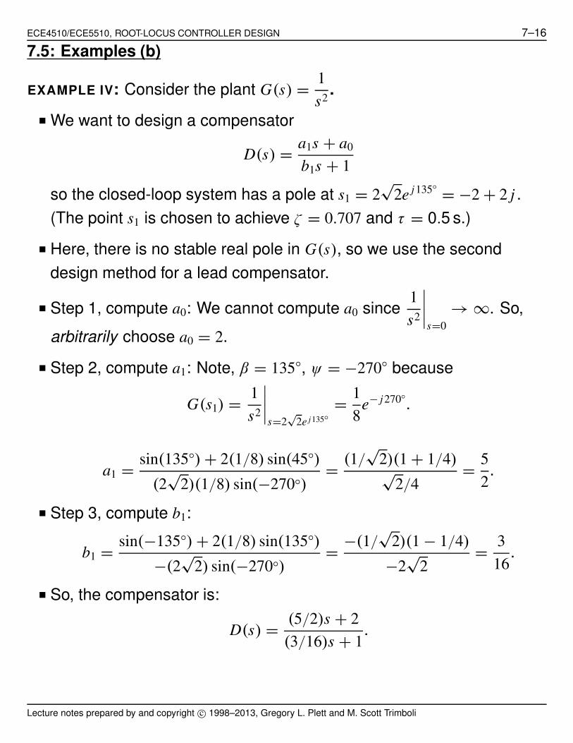
ECE4510/ECE5510, ROOT-LOCUS CONTROLLER DESIGN 7–17
−6 −5 −4 −3 −2 −1 0 1−4
−3
−2
−1
0
1
2
3
4
Real Axis
Imag
Axi
s
Example locus passing through (-2,2)
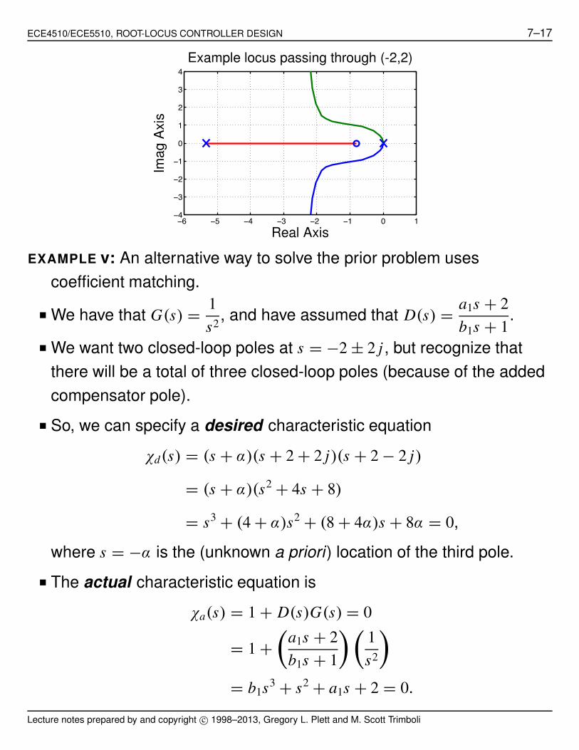
EXAMPLE v: An alternative way to solve the prior problem usescoefficient matching.
! We have that G(s) = 1s2 , and have assumed that D(s) = a1s + 2
b1s + 1.
! We want two closed-loop poles at s = $2 ± 2 j , but recognize thatthere will be a total of three closed-loop poles (because of the addedcompensator pole).
! So, we can specify a desired characteristic equation
(d(s) = (s + ))(s + 2 + 2 j)(s + 2 $ 2 j)
= (s + ))(s2 + 4s + 8)
= s3 + (4 + ))s2 + (8 + 4))s + 8) = 0,
where s = $) is the (unknown a priori) location of the third pole.
! The actual characteristic equation is
(a(s) = 1 + D(s)G(s) = 0
= 1 +*
a1s + 2b1s + 1
+ *1s2
+
= b1s3 + s2 + a1s + 2 = 0.
Lecture notes prepared by and copyright c! 1998–2013, Gregory L. Plett and M. Scott Trimboli
ECE4510/ECE5510, ROOT-LOCUS CONTROLLER DESIGN 7–18
! The coefficient-matching method forces the polynomial coefficients ofthe desired and actual characteristic equations to be the same.
! Looking at the s3 coefficients, we could set b1 = 1, but then we wouldhave problems because we cannot simultaneously have
4 + ) = 1 and 8) = 2.
! So, we divide (a(s) by b1, without changing its meaning:
(a(s) = s3 + 1b1
s2 + a1
b1s + 2
b1= 0.
! This has given us another degree of freedom when solving. Now, wehave
4 + ) = 1b1
, 8 + 4) = a1
b1and 8) = 2
b1.
! Combining the first and third equations gives
2(4 + )) = 8)
8 = 6)
) = 43
.
! With this value of ), we have b1 = 3/16 and a1 = 5/2, as before.
EXAMPLE VI: Consider the compensated system of Example III.
G(s) = 1.1s(s + 1.1)
.
! We like the transient response (so want to leave it alone), but wish toimprove the steady-state response by a factor of 10.
! This calls for a lag controller. Recall that
Kafter = (z0/p0) Kbefore,
so, we want z0/p0 ( 10.
Lecture notes prepared by and copyright c! 1998–2013, Gregory L. Plett and M. Scott Trimboli

ECE4510/ECE5510, ROOT-LOCUS CONTROLLER DESIGN 7–19
! Choose p0 = 0.001. Then, z0 = 0.01 and D(z) = s + 0.01s + 0.001
.
−1 −0.8 −0.6 −0.4 −0.2 0−1.5
−1
−0.5
0
0.5
1
1.5
Real Axis
Imag
Axi
s
Lag shifts locus slightly to the right
! Plots of error versus time without and with the new lag compensator(simulated using Simulink):
0 5 10 15 20 250
0.002
0.004
0.006
0.008
0.01
0.012
0.014
Err
or
Time (s)
Uncompensated
0 200 400 600 800 10000
0.002
0.004
0.006
0.008
0.01
0.012
0.014
Err
or
Time (s)
With lag compensator
! Notice the different time scales: The lag adds a small-amplitude slowtime constant to the output.
Lecture notes prepared by and copyright c! 1998–2013, Gregory L. Plett and M. Scott Trimboli
ECE4510/ECE5510, ROOT-LOCUS CONTROLLER DESIGN 7–20
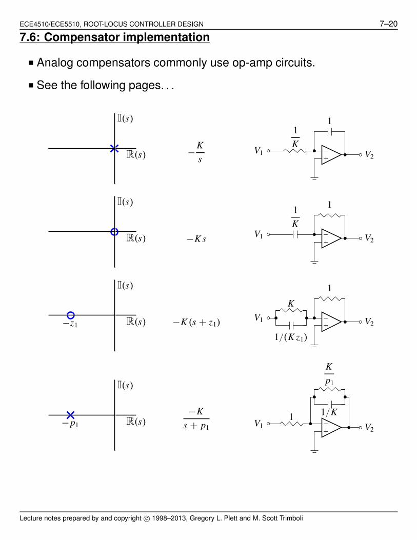
7.6: Compensator implementation
! Analog compensators commonly use op-amp circuits.
! See the following pages. . .
R(s)
I(s)
$Ks
1K
1
V1 V2
R(s)
I(s)
$K s
1K
1
V1 V2
$z1 R(s)
I(s)
$K (s + z1)
K1
1/(K z1)
V1 V2
$p1 R(s)
I(s)
$Ks + p1
1/K1
Kp1
V1 V2
Lecture notes prepared by and copyright c! 1998–2013, Gregory L. Plett and M. Scott Trimboli

ECE4510/ECE5510, ROOT-LOCUS CONTROLLER DESIGN 7–21
$p1 R(s)
I(s)
$K ss + p1
K
1Kp1
V1 V2
R(s)
I(s)
or
$Ks + z1
s + p1
any p1 and z1
1/K
1
1z1
Kp1
V1 V2
R(s)
I(s)
or
$Ks + z1
s + p1
K = K1
K2
any p1 and z1
K1
K2V1 V2
1K1z1
1K2 p1
R(s)
I(s)
s + z1
s + p1
z1 > p1
1
V1 V2
1z1 $ p1
1p1 LAG
R(s)
I(s)
s + z1
s + p1
z1 > p1
1
V1 V2
1p1
1z1 $ p1
LAG
Lecture notes prepared by and copyright c! 1998–2013, Gregory L. Plett and M. Scott Trimboli

ECE4510/ECE5510, ROOT-LOCUS CONTROLLER DESIGN 7–22
R(s)
I(s)K
s + z1
s + p1
p1 > z1
K = p1
z1
1
V1 V2
p1 $ z1
z11p1 LEAD
R(s)
I(s)K
s + z1
s + p1
p1 > z1
K = p1
z1
1
V1 V2
1p1
p1 $ z1
p1LEAD
$z1 R(s)
I(s)
K (s + z1)
K = 1z1
1
V1 V2
1z1
LEAD
Lecture notes prepared by and copyright c! 1998–2013, Gregory L. Plett and M. Scott Trimboli
Related Documents